tes9e_ch02

8/7/2019 tes9e_ch02

http://slidepdf.com/reader/full/tes9ech02 1/102

Slide 1

Copyright © 2004 Pearson Education, Inc.

8/7/2019 tes9e_ch02


Slide 2


Chapter 2Describing, Exploring, and

Comparing Data2-1 Overview

2-2 Frequency Distributions

2-3 Visualizing Data

2-4 Measures of Center

2-5 Measures of Variation

2-6 Measures of Relative Standing2-7 Exploratory Data Analysis

8/7/2019 tes9e_ch02


Slide 3


Created by Tom Wegleitner, Centreville, Virginia

Section 2-1Overview

8/7/2019 tes9e_ch02


Slide 4


D escriptive Statistics

summarize or describe the important

characteristics of a known set of population data

Inferential Statisticsuse sample data to make inferences (or generalizations) about a population

Overview

8/7/2019 tes9e_ch02


Slide 5


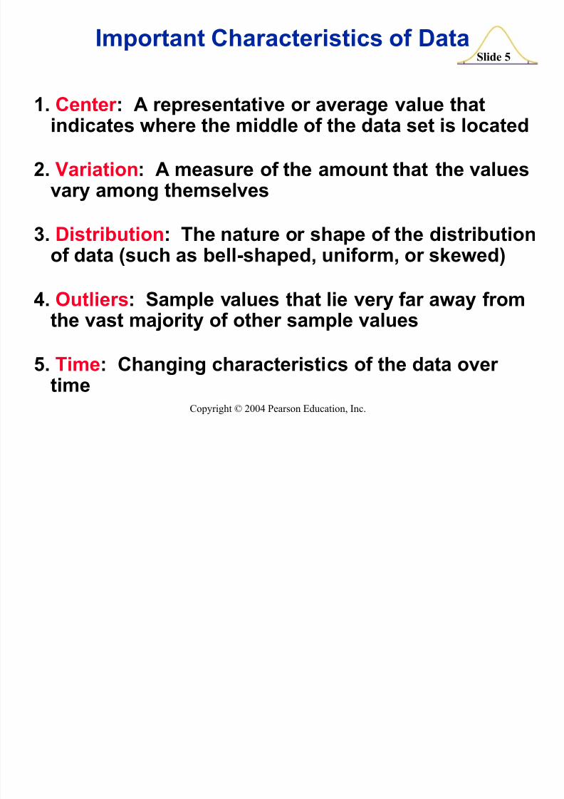
1. Center : A representative or average value thatindicates where the middle of the data set is located

2. Variation : A measure of the amount that the values

vary among themselves

3. D istribution : The nature or shape of the distributionof data (such as bell-shaped, uniform, or skewed)

4. Outliers : Sample values that lie very far away fromthe vast majority of other sample values

5. Time : Changing characteristics of the data over

time

Important Characteristics of D ata

8/7/2019 tes9e_ch02


Slide 6



Section 2-2Frequency D istributions

8/7/2019 tes9e_ch02


Slide 7


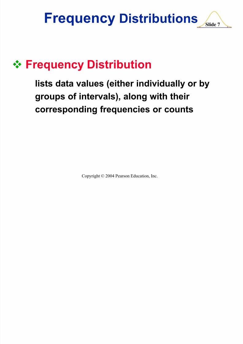
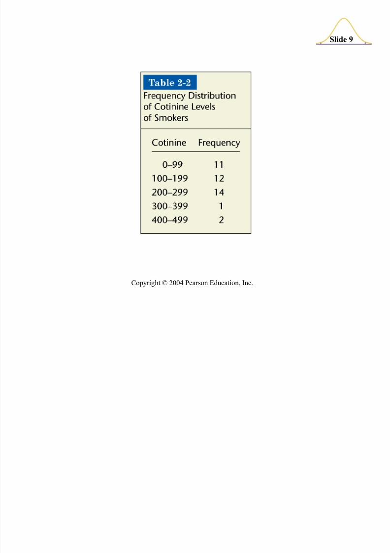
Frequency D istribution

lists data values (either individually or bygroups of intervals), along with their corresponding frequencies or counts

Frequency D istributions

8/7/2019 tes9e_ch02


Slide 8


8/7/2019 tes9e_ch02


Slide 9


8/7/2019 tes9e_ch02


Slide 10


Frequency D istributions

Definitions

8/7/2019 tes9e_ch02


8/7/2019 tes9e_ch02


Slide 12


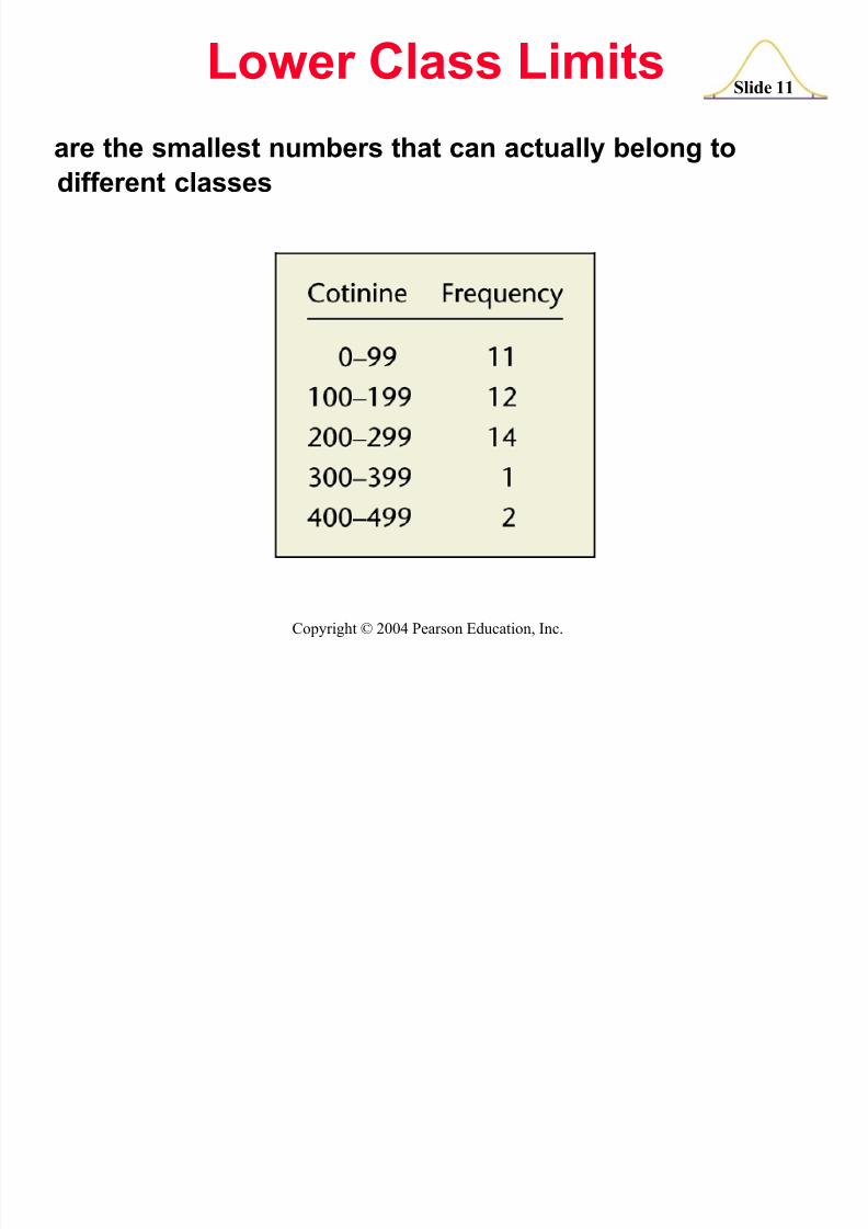
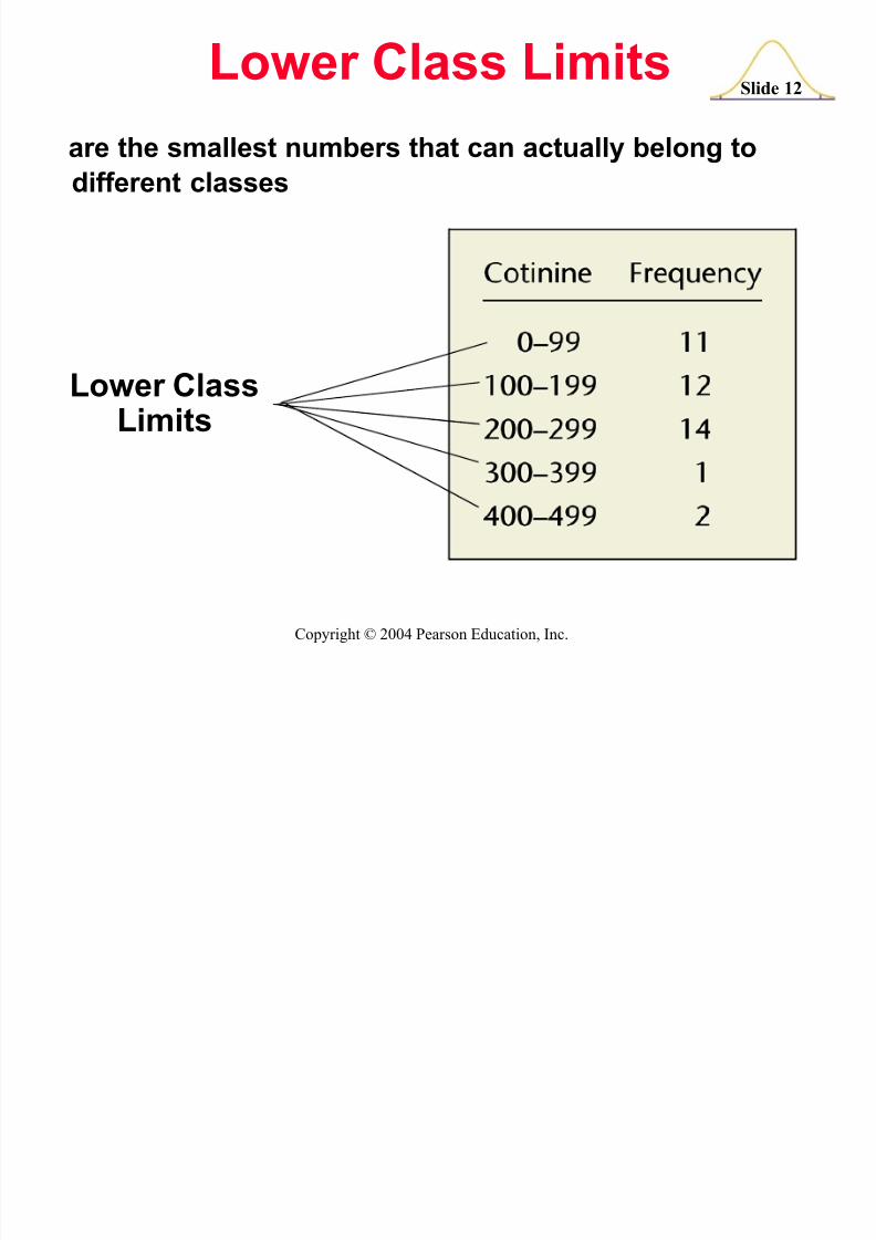
are the smallest numbers that can actually belong todifferent classes

L ower ClassL imits

L ower Class L imits

8/7/2019 tes9e_ch02


Slide 13


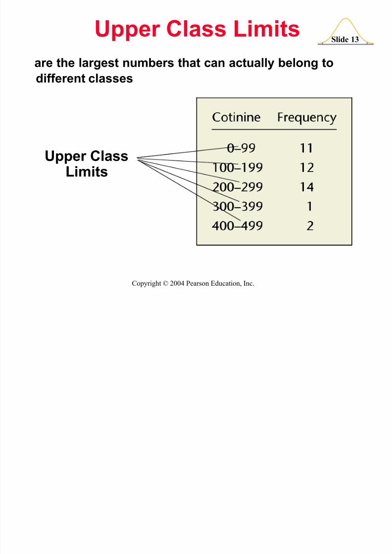
U pper Class L imits

are the largest numbers that can actually belong todifferent classes

U pper ClassL imits

8/7/2019 tes9e_ch02


Slide 14


are the numbers used to separate classes, butwithout the gaps created by class limits

Class Boundaries

8/7/2019 tes9e_ch02


Slide 15


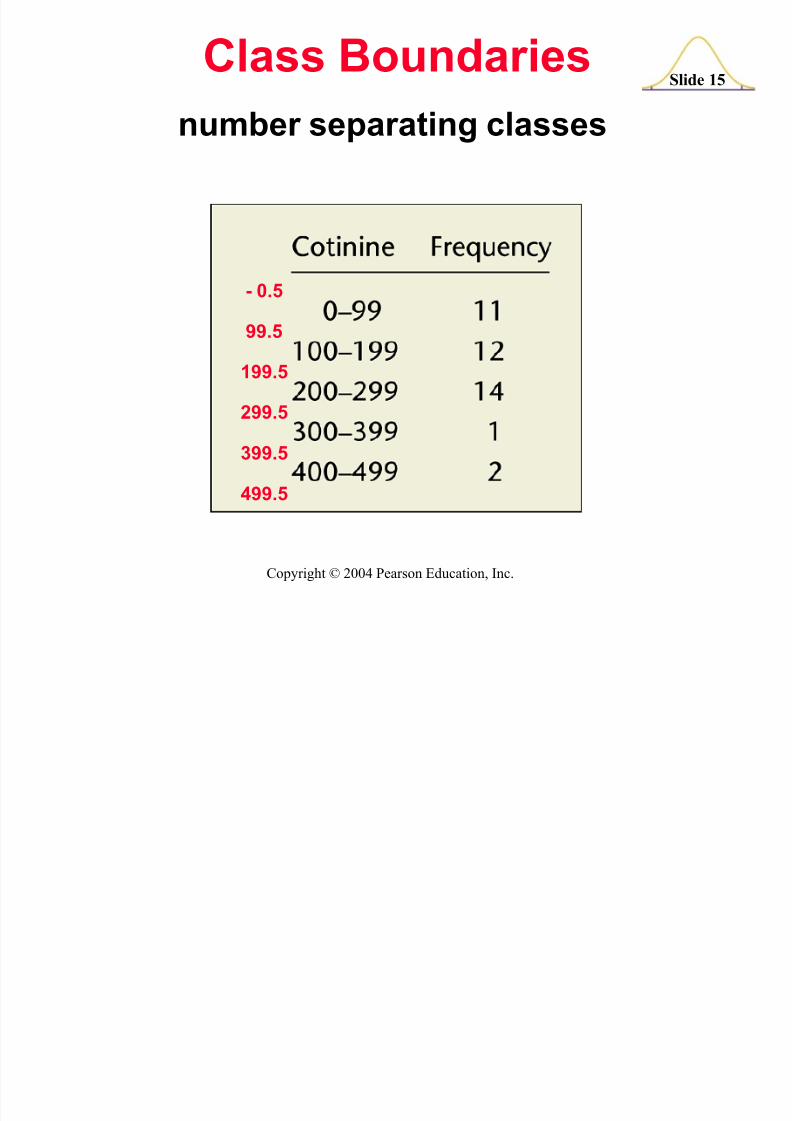
number separating classes

Class Boundaries

- 0.5

99.5

199.5

299.5

399.5

499.5

8/7/2019 tes9e_ch02


Slide 16


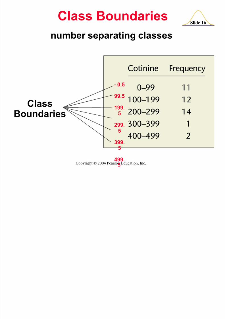
Class Boundaries

number separating classes

Class

Boundaries

- 0.5

99.5

199.5

299.5

399.5

499.

8/7/2019 tes9e_ch02


Slide 17


midpoints of the classes

Class Midpoints

Class midpoints can be found byadding the lower class limit to the

upper class limit and dividing the sumby two.

8/7/2019 tes9e_ch02


Slide 18


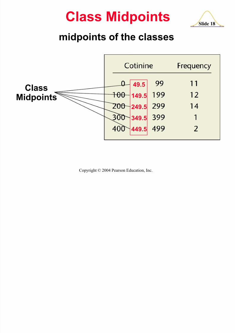
ClassMidpoints

midpoints of the classes

Class Midpoints

49.5

149.5

249.5

349.5

449.5

8/7/2019 tes9e_ch02


Slide 19


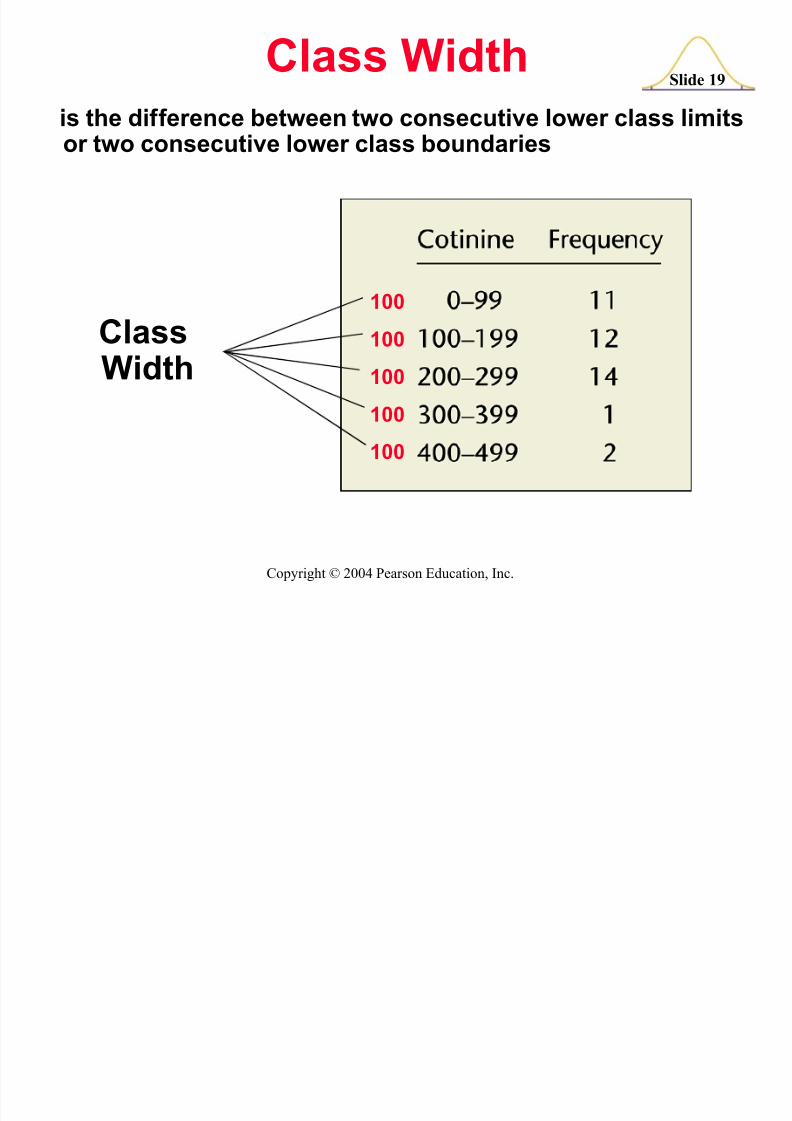
Class Widthis the difference between two consecutive lower class limitsor two consecutive lower class boundaries

ClassWidth

100

100

100

100100

8/7/2019 tes9e_ch02


Slide 20


1. L arge data sets can be summarized.

2. Can gain some insight into the nature of data.

3. Have a basis for constructing graphs.

Reasons for ConstructingFrequency D istributions

8/7/2019 tes9e_ch02


Slide 21


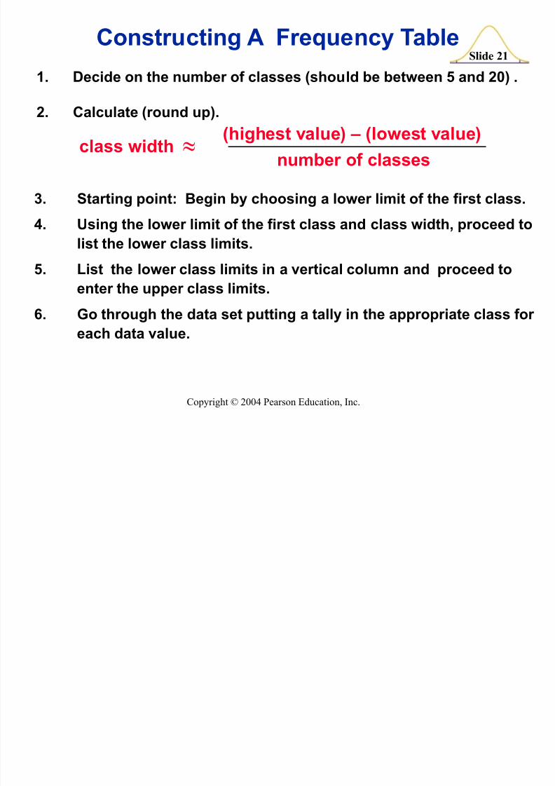
3. Starting point: Begin by choosing a lower limit of the first class.

4. U sing the lower limit of the first class and class width, proceed tolist the lower class limits.

5. L ist the lower class limits in a vertical column and proceed to

enter the upper class limits.6. Go through the data set putting a tally in the appropriate class for

each data value.

Constructing A Frequency Table

1. D ecide on the number of classes (should be between 5 and 20) .

2. Calculate (round up).

class width } (highest value) ± (lowest value)number of classes

8/7/2019 tes9e_ch02


Slide 22


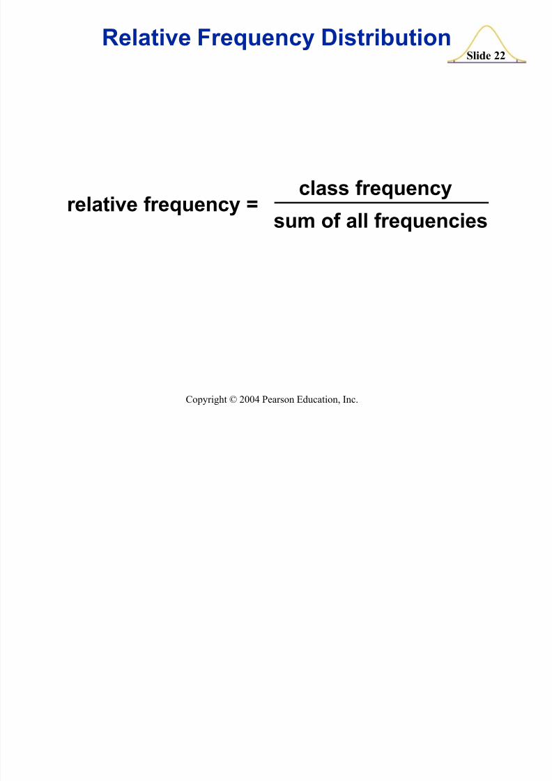
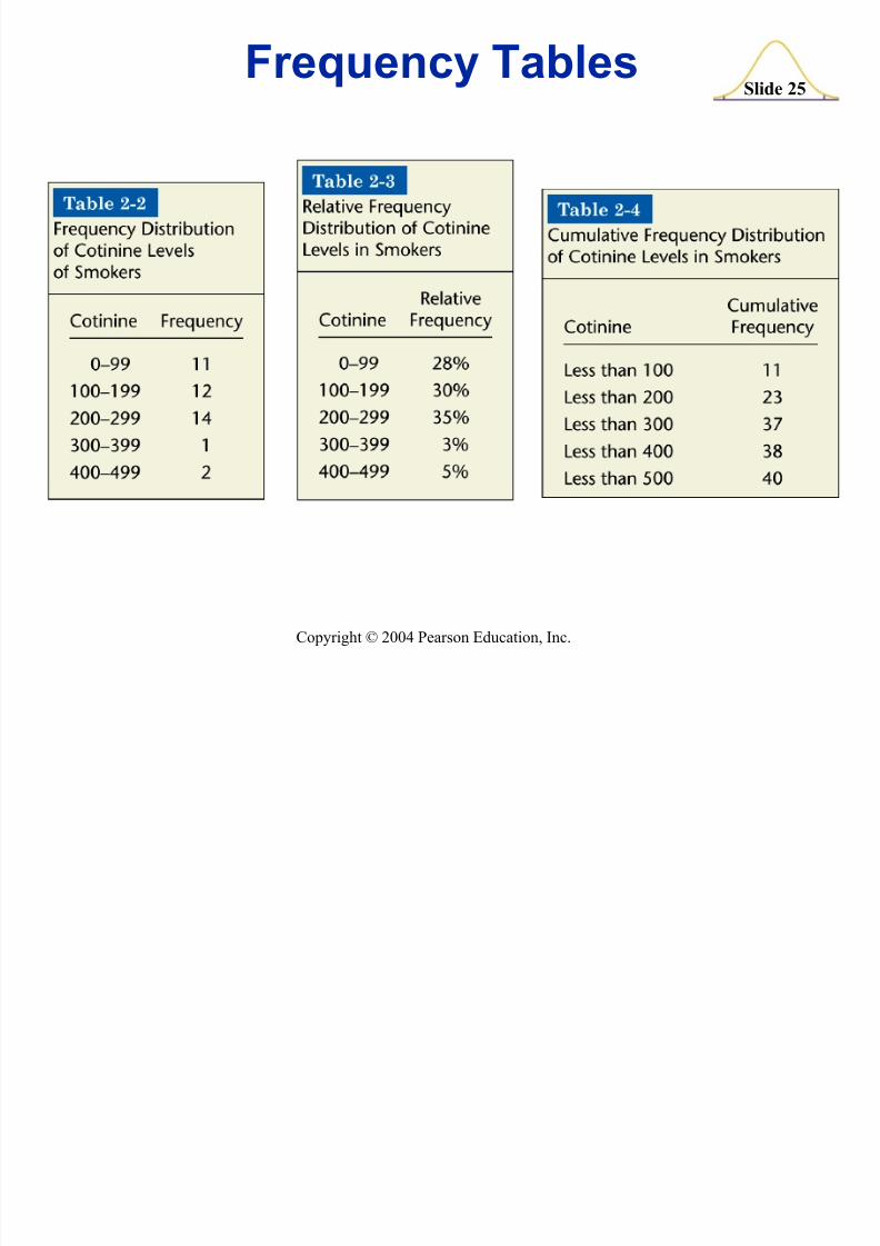
Relative Frequency D istribution

relative frequency = class frequencysum of all frequencies

8/7/2019 tes9e_ch02


Slide 23


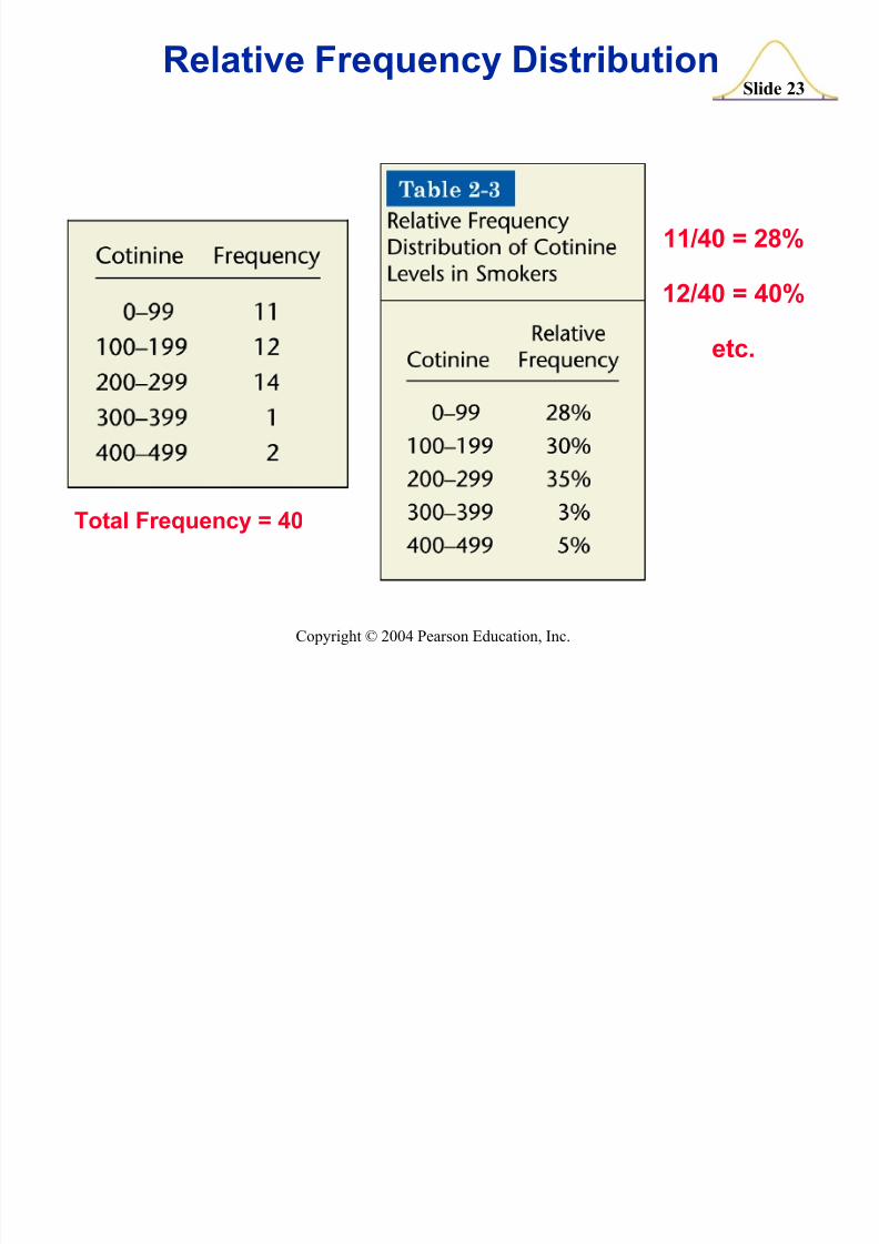
Relative Frequency D istribution

11/40 = 28%

12/40 = 40%

etc.

Total Frequency = 40

8/7/2019 tes9e_ch02


Slide 24


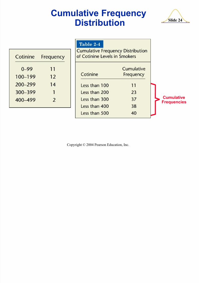
Cumulative FrequencyD istribution

CumulativeFrequencies

8/7/2019 tes9e_ch02


Slide 25


Frequency Tables

8/7/2019 tes9e_ch02


Slide 26


Recap

In this Section we have discussed

Important characteristics of data

Frequency distributionsProcedures for constructing frequency distributions

Relative frequency distributions

Cumulative frequency distributions

8/7/2019 tes9e_ch02


Slide 27



Section 2-3Visualizing D ata

8/7/2019 tes9e_ch02


Slide 28


Visualizing D ata

D epict the nature of shape or shape of the data distribution

8/7/2019 tes9e_ch02


Slide 29


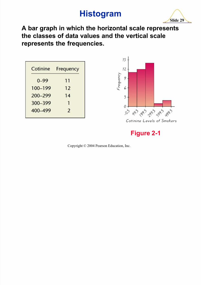
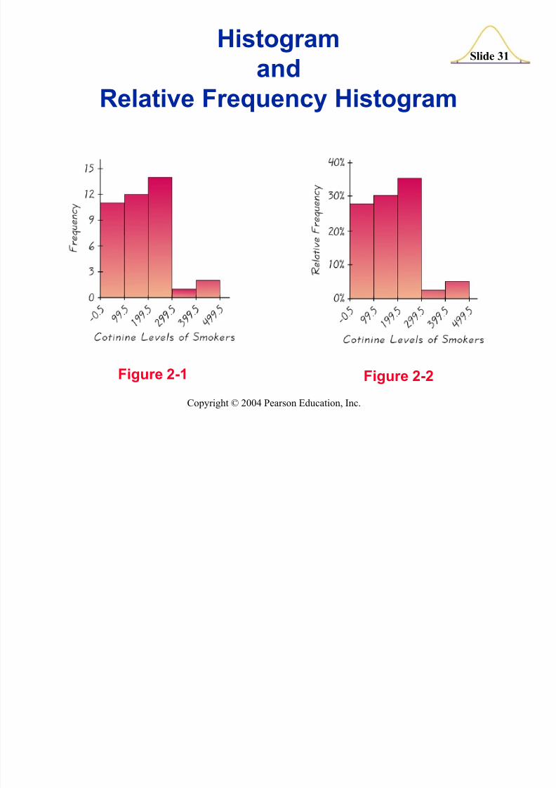
Histogram

A bar graph in which the horizontal scale represents

the classes of data values and the vertical scalerepresents the frequencies.

Figure 2-1

8/7/2019 tes9e_ch02


Slide 30


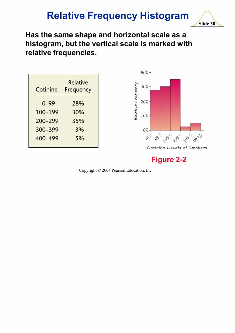
Relative Frequency Histogram

Has the same shape and horizontal scale as ahistogram, but the vertical scale is marked withrelative frequencies.

Figure 2-2

8/7/2019 tes9e_ch02


Slide 31


Histogramand

Relative Frequency Histogram

Figure 2-1 Figure 2-2

8/7/2019 tes9e_ch02


Slide 32


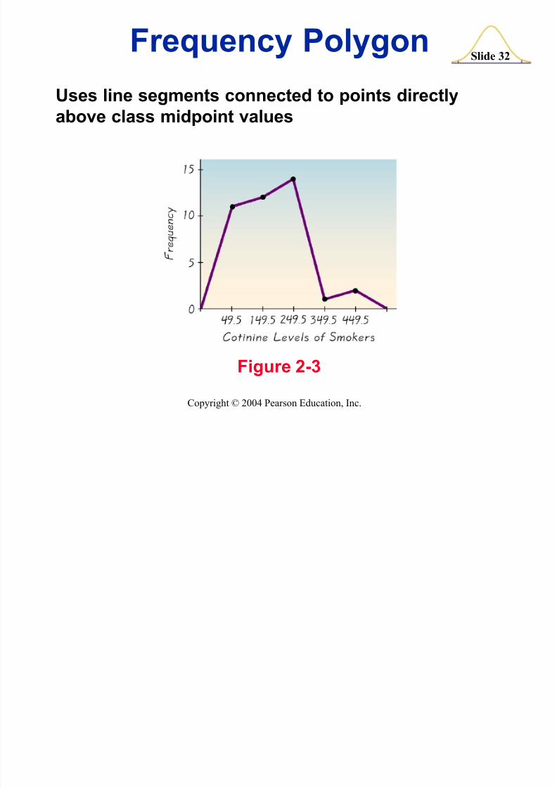
Frequency Polygon

U ses line segments connected to points directlyabove class midpoint values

Figure 2-3

8/7/2019 tes9e_ch02


Slide 33


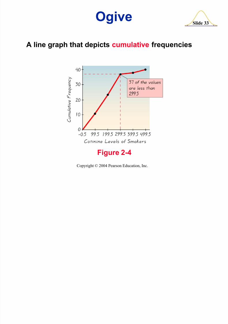
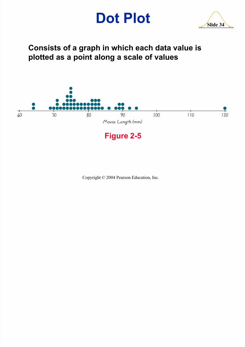
Ogive

A line graph that depicts cumulative frequencies

Figure 2-4

8/7/2019 tes9e_ch02


8/7/2019 tes9e_ch02


Slide 35


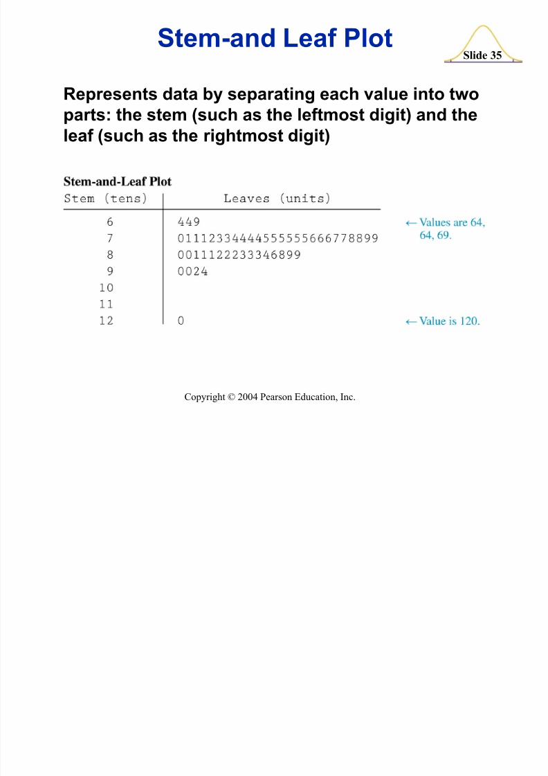
Stem-and L eaf Plot

Represents data by separating each value into twoparts: the stem (such as the leftmost digit) and theleaf (such as the rightmost digit)

8/7/2019 tes9e_ch02


Slide 36


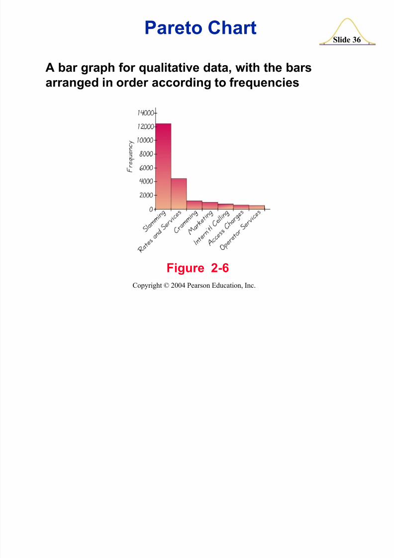
Pareto Chart

A bar graph for qualitative data, with the barsarranged in order according to frequencies

Figure 2-6

8/7/2019 tes9e_ch02


Slide 37


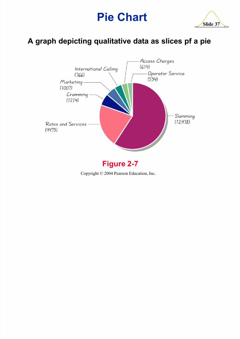
Pie Chart

A graph depicting qualitative data as slices pf a pie

Figure 2-7

8/7/2019 tes9e_ch02


Slide 38


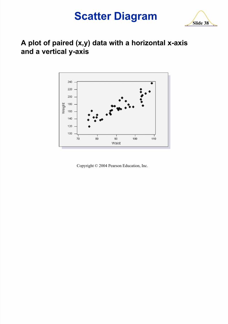
Scatter D iagram

A plot of paired (x,y) data with a horizontal x-axisand a vertical y-axis

8/7/2019 tes9e_ch02


Slide 39


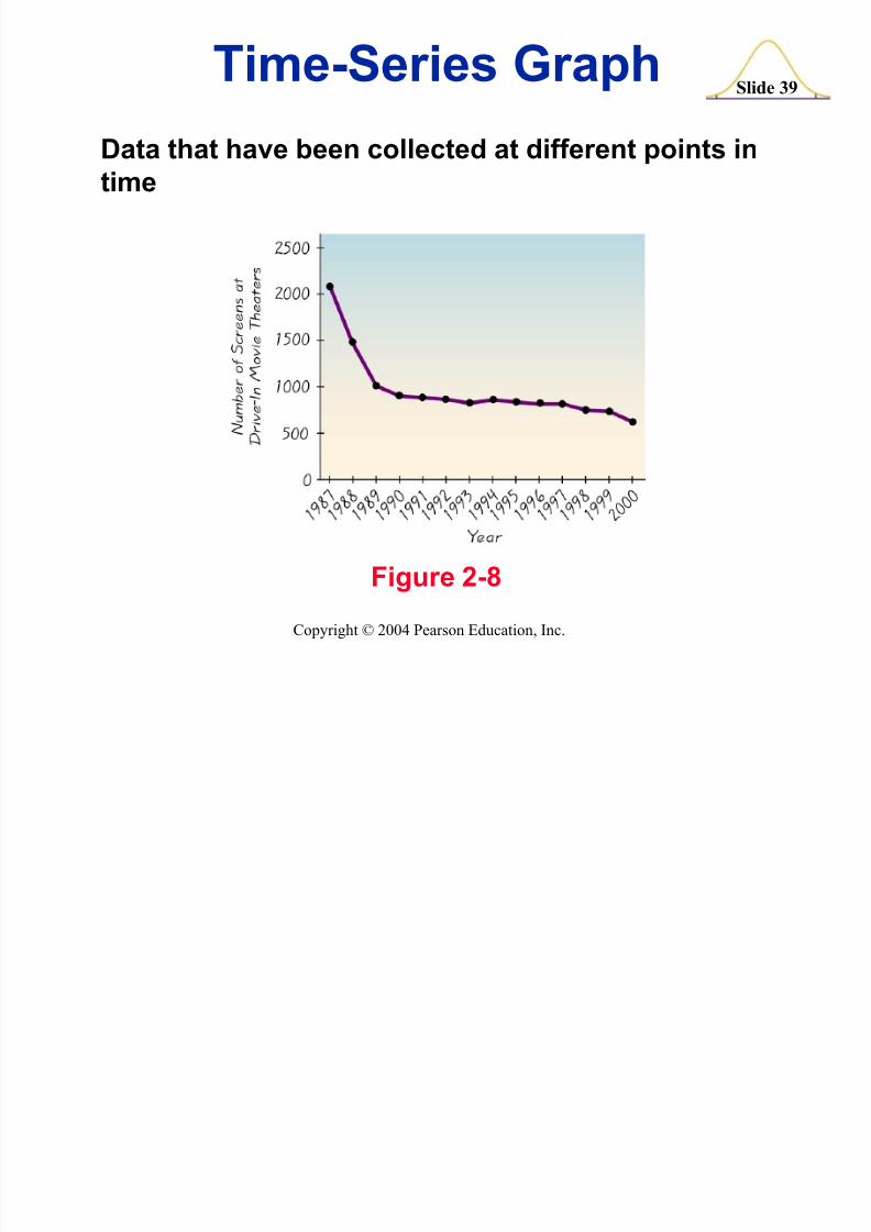
Time-Series Graph

D ata that have been collected at different points intime

Figure 2-8

8/7/2019 tes9e_ch02


Slide 40


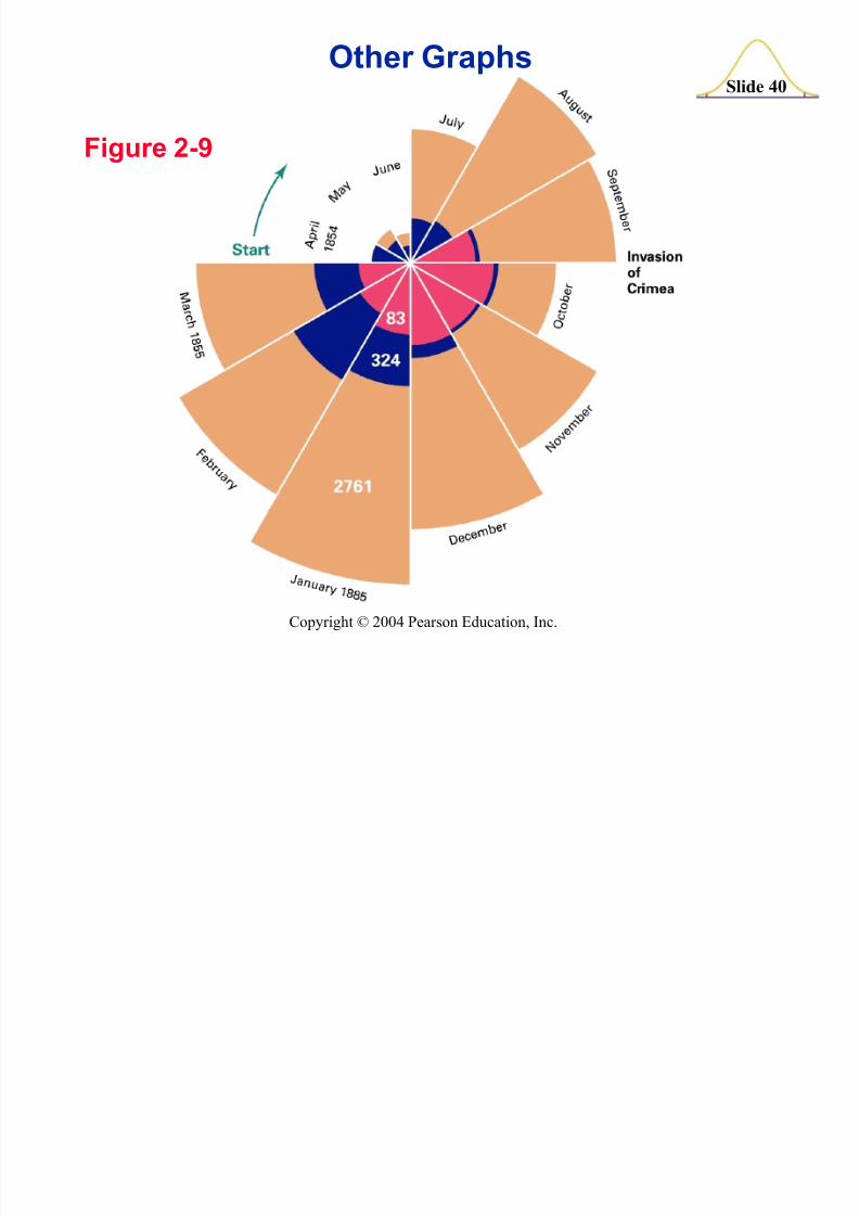
Other Graphs

Figure 2-9

8/7/2019 tes9e_ch02


Slide 41


Recap

In this Section we have discussed graphsthat are pictures of distributions.

Keep in mind that the object of this section isnot just to construct graphs, but to learn

something about the data sets ± that is, tounderstand the nature of their distributions.

8/7/2019 tes9e_ch02


Slide 42



Section 2-4Measures of Center

8/7/2019 tes9e_ch02


Slide 43


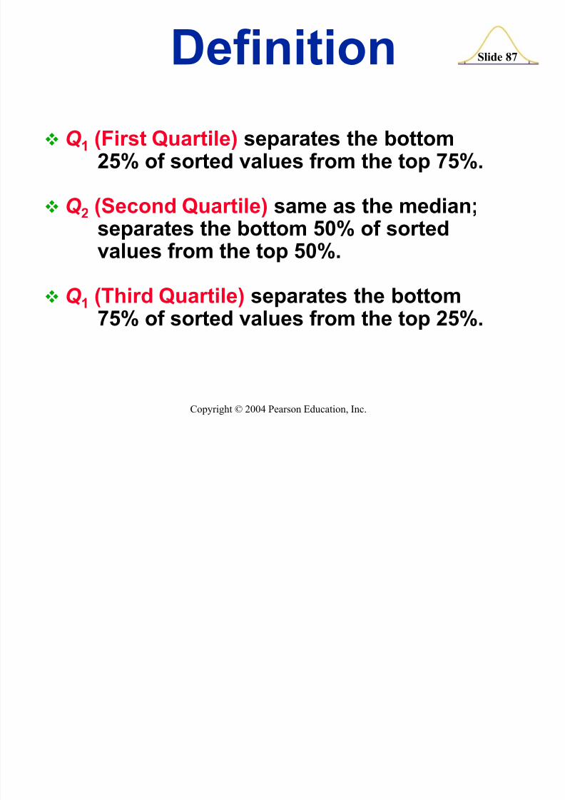
D efinition

Measure of Center The value at the center or middleof a data set

8/7/2019 tes9e_ch02


8/7/2019 tes9e_ch02


Slide 45


N otation

7 denotes the addition of a set of values

x is the variable usually used to represent the individualdata values

n represents the number of values in a sample

N represents the number of values in a population

8/7/2019 tes9e_ch02


Slide 46


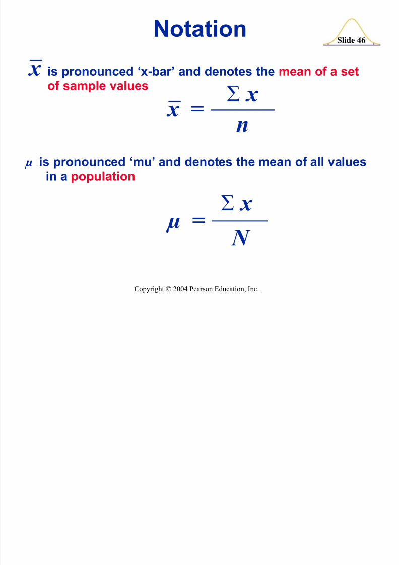
N otation

µ is pronounced µmu¶ and denotes the mean of all valuesin a population

x =n

7 x is pronounced µx-bar¶ and denotes the mean of a setof sample values x

N µ =

7 x

8/7/2019 tes9e_ch02


Slide 47


D efinitionsMedian

the middle value when the originaldata values are arranged in order of

increasing (or decreasing) magnitudeoften denoted by x (pronounced µx-tilde¶)~

is not affected by an extreme value

8/7/2019 tes9e_ch02


Slide 48


Finding the Median

If the number of values is odd, themedian is the number located in theexact middle of the list

If the number of values is even, themedian is found by computing the

mean of the two middle numbers

8/7/2019 tes9e_ch02


Slide 49


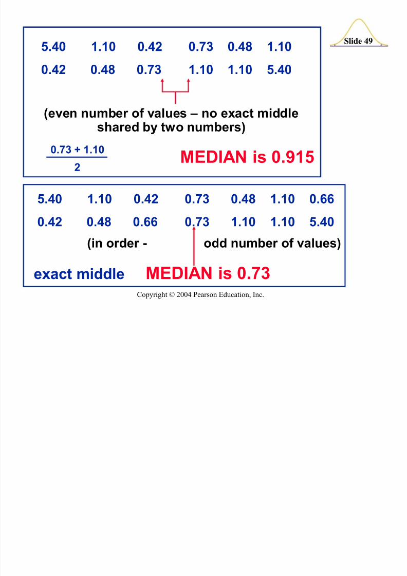
5.40 1.10 0.42 0.73 0.48 1.10 0.66

0.42 0.48 0.66 0.73 1.10 1.10 5.40

(in order - odd number of values)

exact middle MED IAN is 0.73

5.40 1.10 0.42 0.73 0.48 1.10

0.42 0.48 0.73 1.10 1.10 5.40

0.73 + 1.10

2

(even number of values ± no exact middleshared by two numbers)

MED IAN is 0.915

8/7/2019 tes9e_ch02


Slide 50


D efinitionsMode

the value that occurs most frequently

The mode is not always unique. A data set may be:

BimodalMultimodalN o Mode

denoted by Mthe only measure of central tendency that

can be used with nominal data

8/7/2019 tes9e_ch02


Slide 51


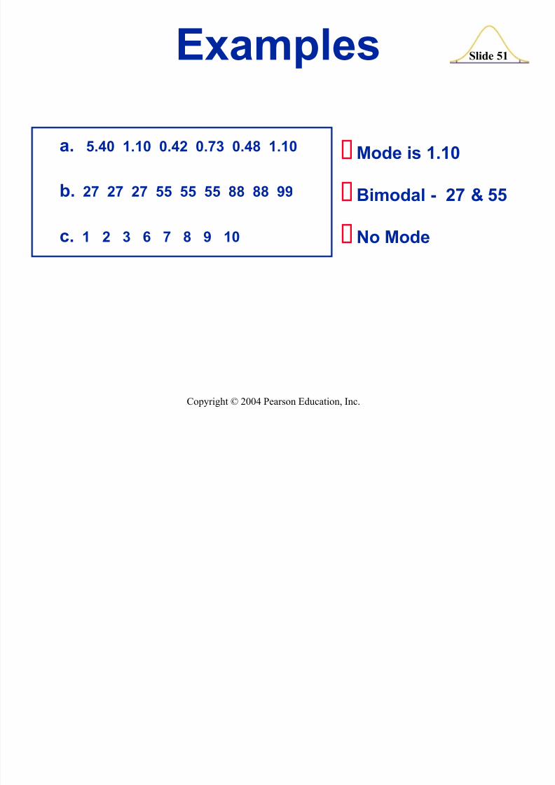
a. 5.40 1.10 0.42 0.73 0.48 1.10

b. 27 27 27 55 55 55 88 88 99

c. 1 2 3 6 7 8 9 10

Examples

Mode is 1.10

Bimodal - 27 & 55

N o Mode

8/7/2019 tes9e_ch02


Slide 52


Midrange

the value midway between the highestand lowest values in the original dataset

D efinitions

Midrange = highest score + lowest score

2

8/7/2019 tes9e_ch02


Slide 53


Carry one more decimal place than ispresent in the original set of values

Round-off Rule for Measures of Center

8/7/2019 tes9e_ch02


Slide 54


Assume that in each class, all samplevalues are equal to the class

midpoint

Mean from a FrequencyD istribution

8/7/2019 tes9e_ch02


Slide 55


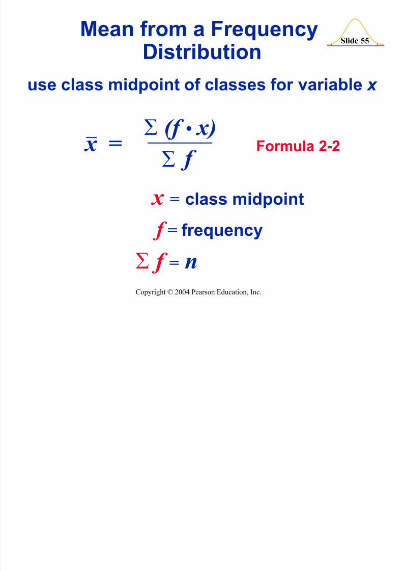
use class midpoint of classes for variable x

Mean from a FrequencyD istribution

x = class midpoint

f = frequency

7 f = n

x = Formula 2-2 f

7 ( f x)7

8/7/2019 tes9e_ch02


Slide 56


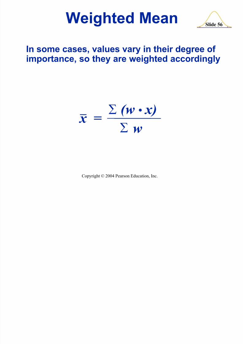
Weighted Mean

x =

w

7 (w x)

7

In some cases, values vary in their degree of importance, so they are weighted accordingly

8/7/2019 tes9e_ch02


Slide 57


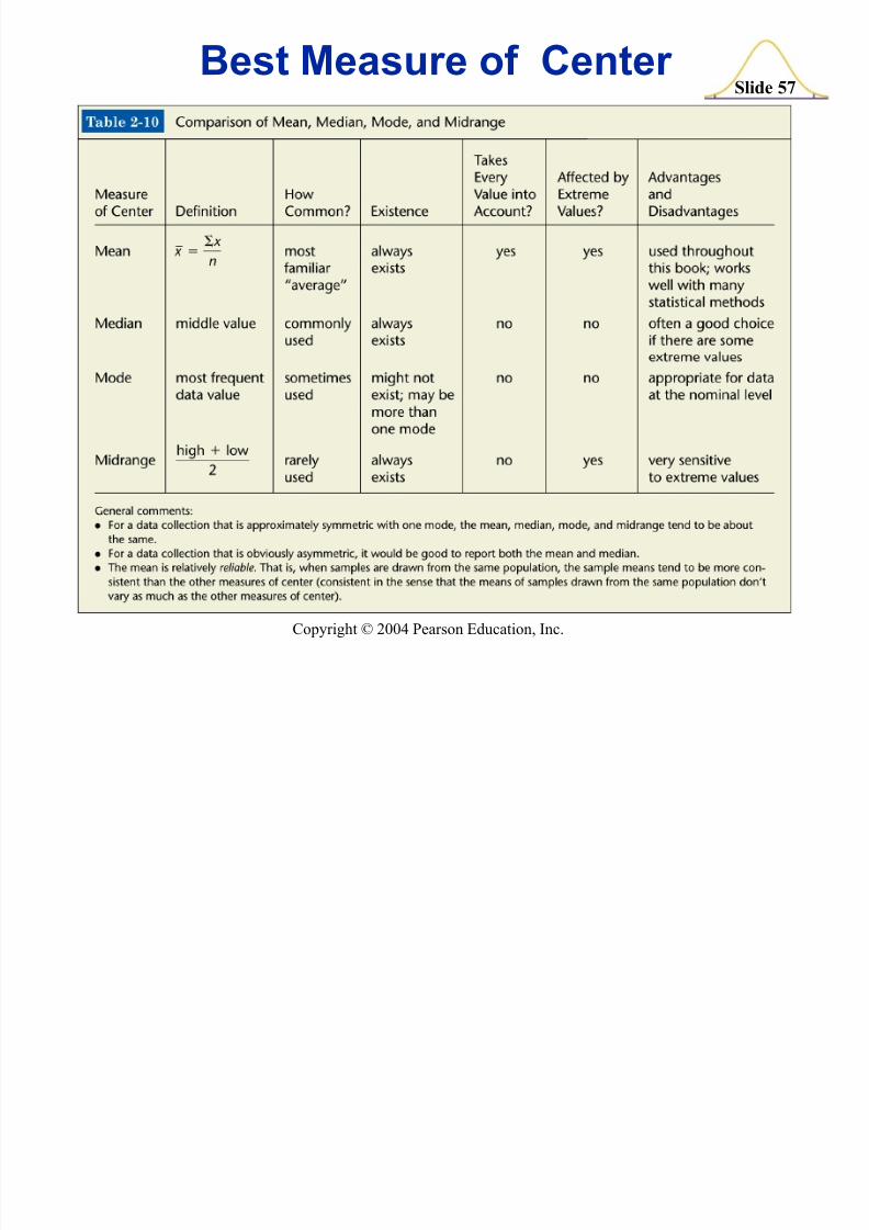
Best Measure of Center

8/7/2019 tes9e_ch02


Slide 58


SymmetricD ata is symmetric if the left half of its

histogram is roughly a mirror image of its right half.

SkewedD ata is skewed if it is not symmetricand if it extends more to one side thanthe other.

D efinitions

8/7/2019 tes9e_ch02


Slide 59


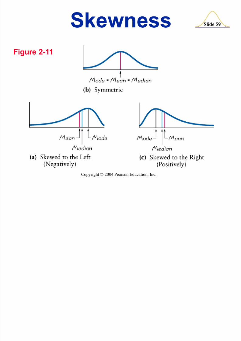
SkewnessFigure 2-11

8/7/2019 tes9e_ch02


Slide 60


RecapIn this section we have discussed:

Types of Measures of Center MeanMedian

Mode

Mean from a frequency distribution

Weighted means

Best Measures of Center

Skewness

8/7/2019 tes9e_ch02


Slide 61



Section 2-5Measures of Variation

8/7/2019 tes9e_ch02


Slide 62


Measures of Variation

Because this section introduces the conceptof variation, this is one of the most importantsections in the entire book

8/7/2019 tes9e_ch02


Slide 63


D efinition

The range of a set of data is thedifference between the highestvalue and the lowest value

valuehighest lowestvalue

D f

8/7/2019 tes9e_ch02


Slide 64


D efinition

The standard deviation of a set of sample values is a measure of variation of values about the mean

8/7/2019 tes9e_ch02


S l S d d D i i

8/7/2019 tes9e_ch02


Slide 66


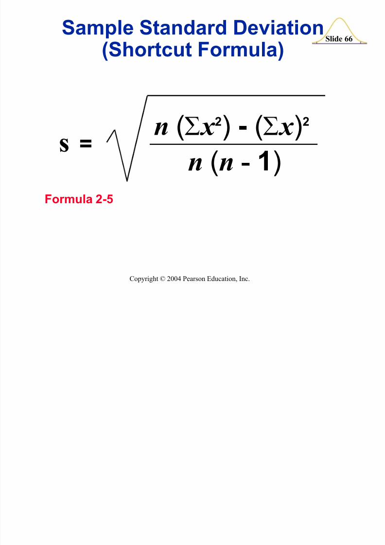
Sample Standard D eviation(Shortcut Formula)

Formula 2-5

n (n - 1)s = n (

7 x

2

) - (7 x )

2

St d d D i ti

8/7/2019 tes9e_ch02


Slide 67


Standard D eviation -Key Points

The standard deviation is a measure of variation of all values from the mean

The value of the standard deviation s is usuallypositive

The value of the standard deviation s can increasedramatically with the inclusion of one or more

outliers (data values far away from all others)

The units of the standard deviation s are the same asthe units of the original data values

8/7/2019 tes9e_ch02


D fi i i

8/7/2019 tes9e_ch02


Slide 69


Population variance: Square of the populationstandard deviation W

D efinition

The variance of a set of values is a measure of variation equal to the square of the standarddeviation.

Sample variance: Square of the sample standarddeviation s

V i N i

8/7/2019 tes9e_ch02


Slide 70


Variance - N otation

standard deviation squared

sW

2

2 }N otationSample variance

Population variance

R d ff R l

8/7/2019 tes9e_ch02


Slide 71


Round-off Rulefor Measures of Variation

Carry one more decimal place thanis present in the original set of data.

Round only the final answer, not values in

the middle of a calculation.

8/7/2019 tes9e_ch02


St d d D i ti f

8/7/2019 tes9e_ch02


Slide 73


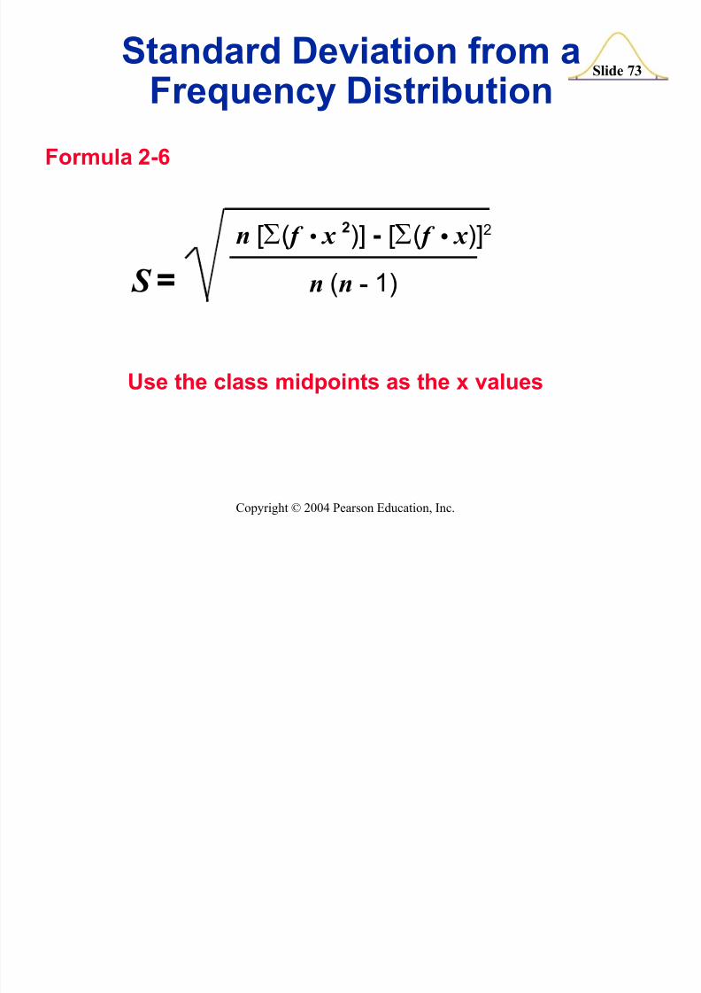
Standard D eviation from aFrequency D istribution

U se the class midpoints as the x values

Formula 2-6

n (n - 1) S =n [7

( f x 2

)]- [7

( f x

)]2

Estimation of Standard

8/7/2019 tes9e_ch02


Slide 74


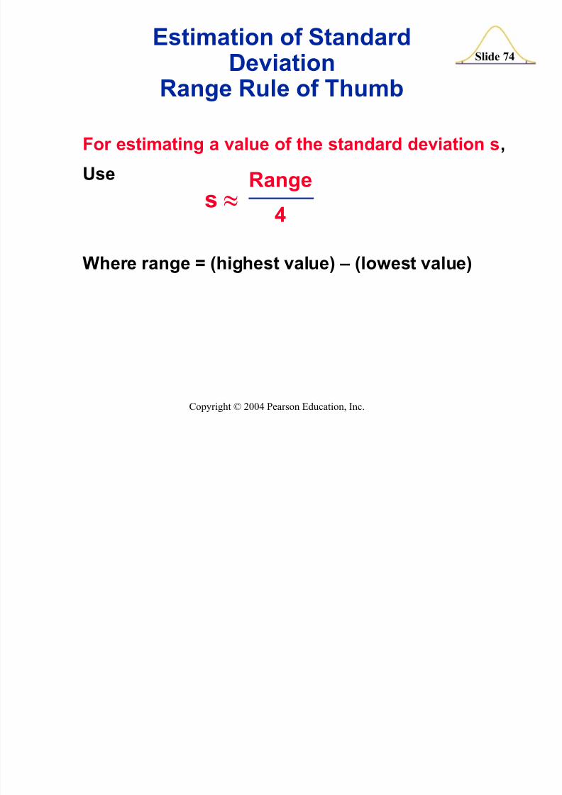
Estimation of StandardD eviation

Range Rule of Thumb

For estimating a value of the standard deviation s ,

U se

Where range = (highest value) ± (lowest value)

Range

4s }

Estimation of Standard

8/7/2019 tes9e_ch02


Slide 75


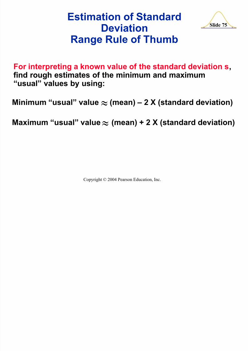
Estimation of StandardD eviation

Range Rule of Thumb

For interpreting a known value of the standard deviation s ,find rough estimates of the minimum and maximum³usual´ values by using:

Minimum ³usual´ value (mean) ± 2 X (standard deviation)}

Maximum ³usual´ value (mean) + 2 X (standard deviation)}

D efinition

8/7/2019 tes9e_ch02


Slide 76


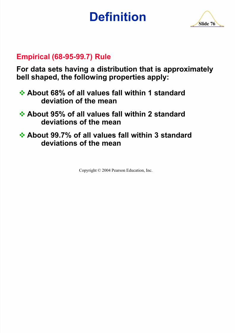
D efinition

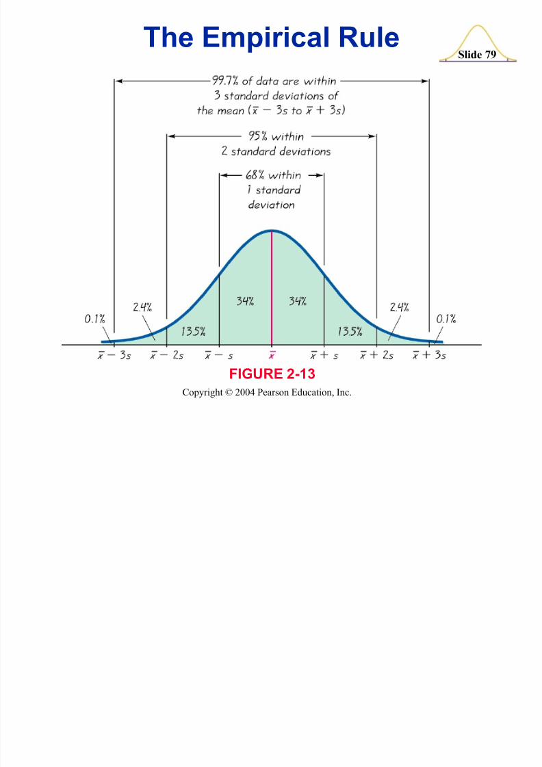
Empirical (68-95-99.7) Rule

For data sets having a distribution that is approximatelybell shaped, the following properties apply:

About 68% of all values fall within 1 standarddeviation of the mean

About 95% of all values fall within 2 standarddeviations of the mean

About 99.7% of all values fall within 3 standarddeviations of the mean

The Empirical Rule

8/7/2019 tes9e_ch02


Slide 77


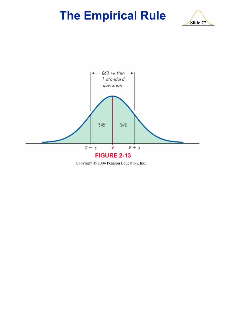
The Empirical Rule

FIG U RE 2-13

The Empirical Rule

8/7/2019 tes9e_ch02


Slide 78


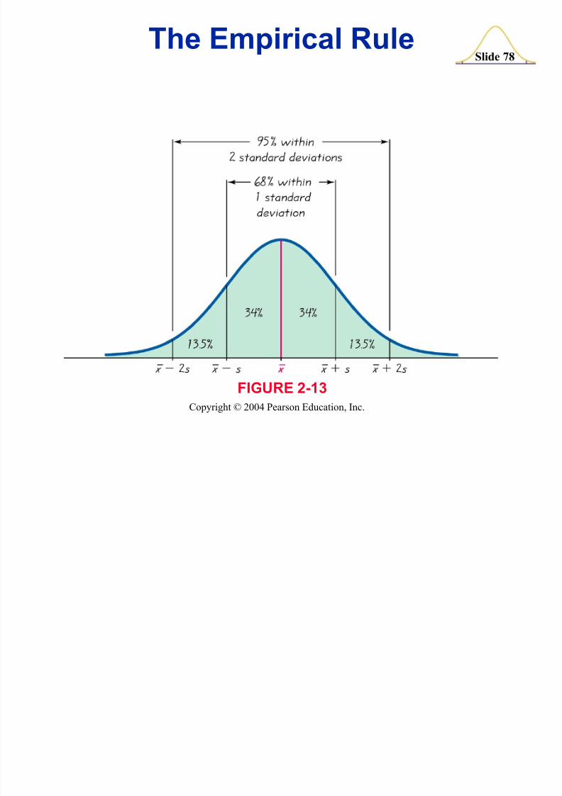
The Empirical Rule

FIG U RE 2-13

8/7/2019 tes9e_ch02


D efinition

8/7/2019 tes9e_ch02


Slide 80


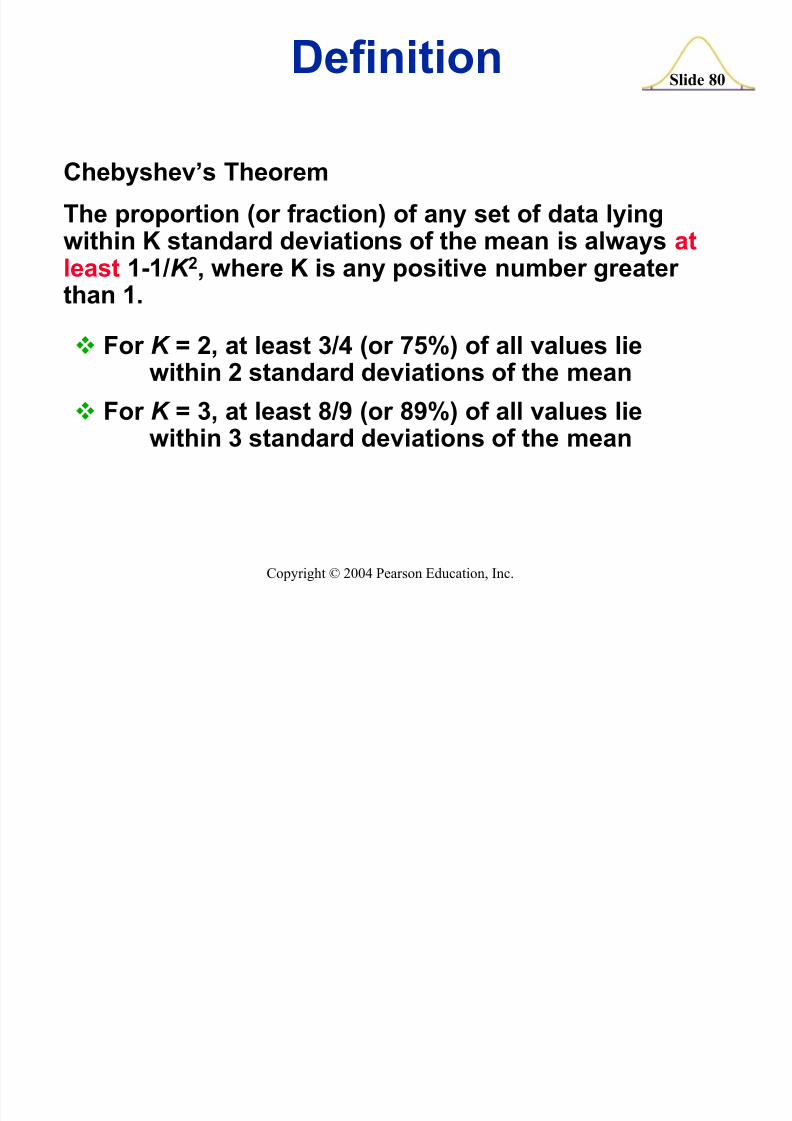
D efinition

Chebyshev¶s Theorem

The proportion (or fraction) of any set of data lyingwithin K standard deviations of the mean is always atleast 1-1/ K 2, where K is any positive number greater than 1.

For K = 2, at least 3/4 (or 75%) of all values liewithin 2 standard deviations of the mean

For K = 3, at least 8/9 (or 89%) of all values liewithin 3 standard deviations of the mean

8/7/2019 tes9e_ch02


Recap

8/7/2019 tes9e_ch02


Slide 82


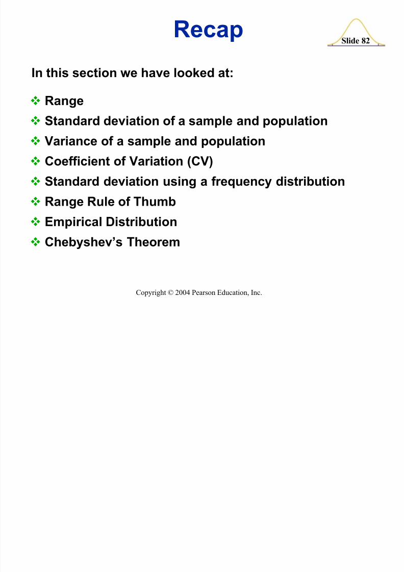
Recap

In this section we have looked at:Range

Standard deviation of a sample and population

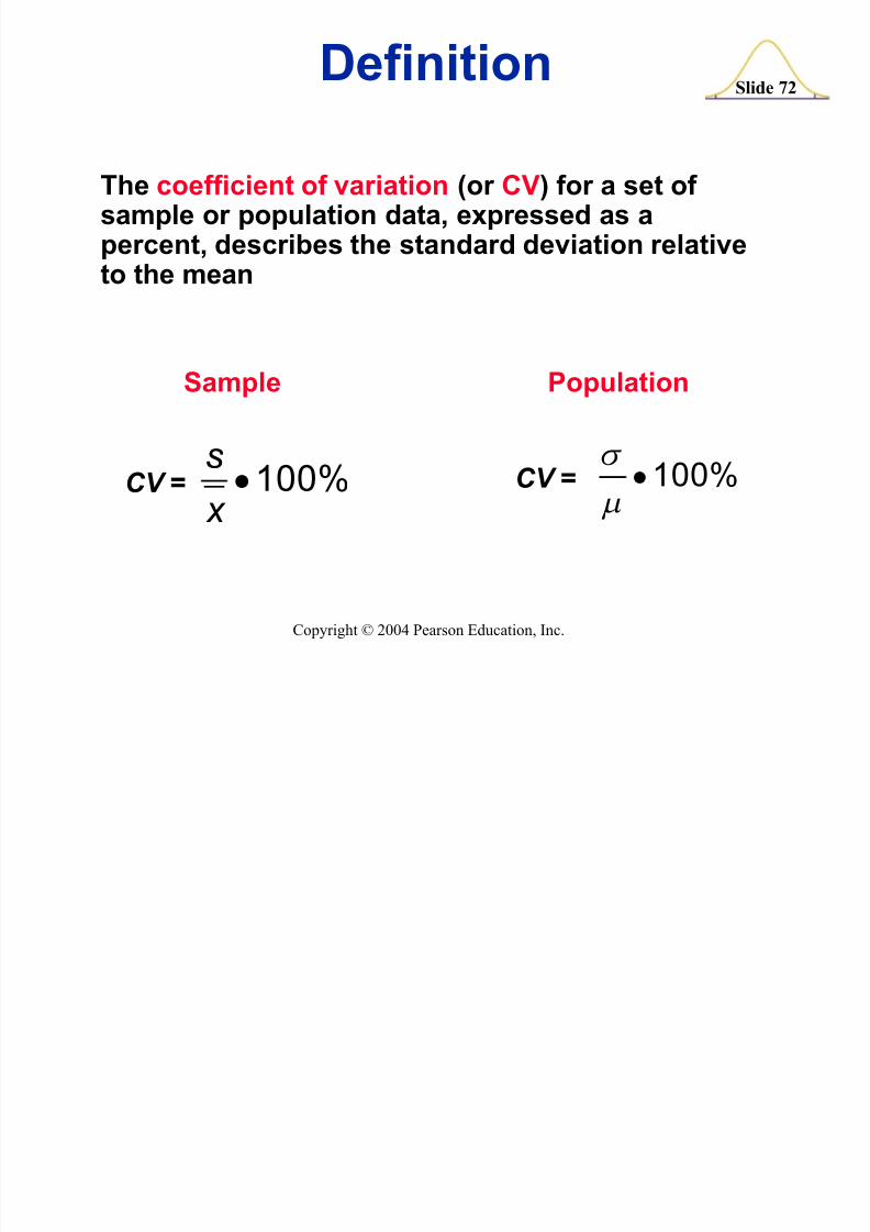
Variance of a sample and populationCoefficient of Variation (CV)

Standard deviation using a frequency distribution

Range Rule of Thumb

Empirical D istributionChebyshev¶s Theorem

8/7/2019 tes9e_ch02


Slide 83



Section 2-6Measures of Relative

Standing

D efinition

8/7/2019 tes9e_ch02


Slide 84


z Score (or standard score)

the number of standard deviationsthat a given value x is above or belowthe mean.

D efinition

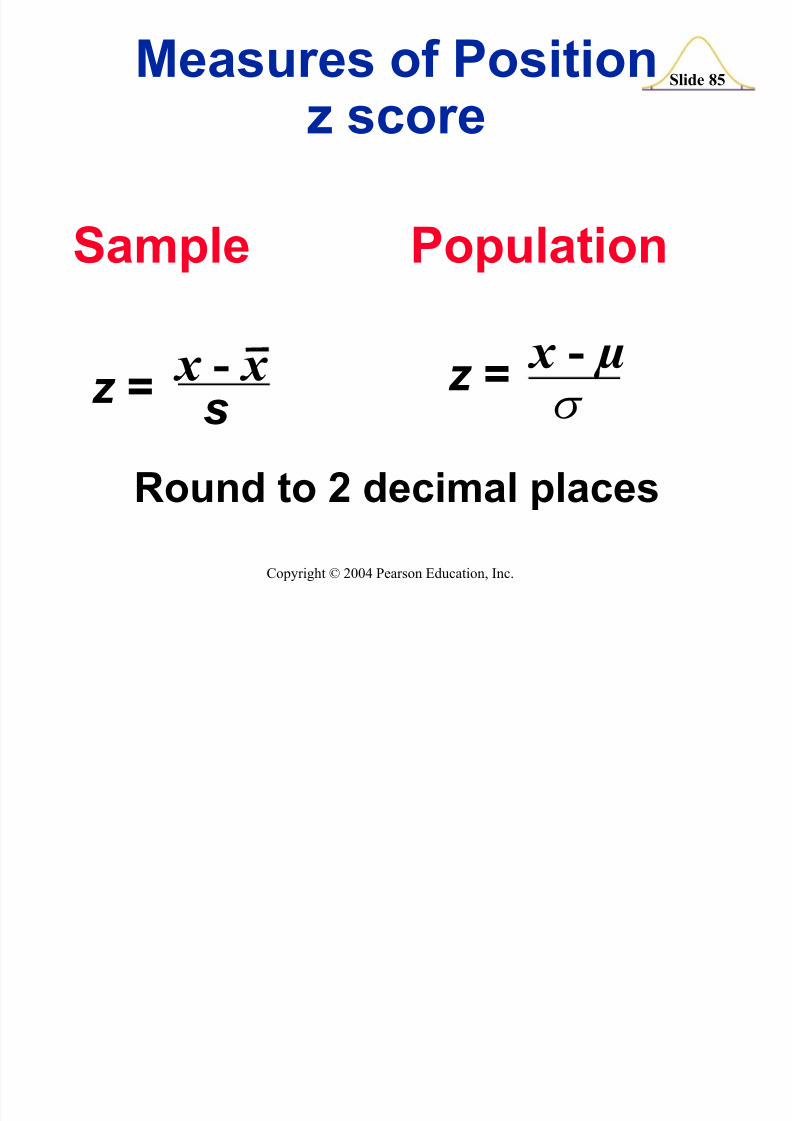
Measures of Position

8/7/2019 tes9e_ch02


Slide 85


Sample Population

x - µz =W

Round to 2 decimal places

Measures of Positionz score

z = x - x

s

Interpreting Z Scores

8/7/2019 tes9e_ch02


Slide 86


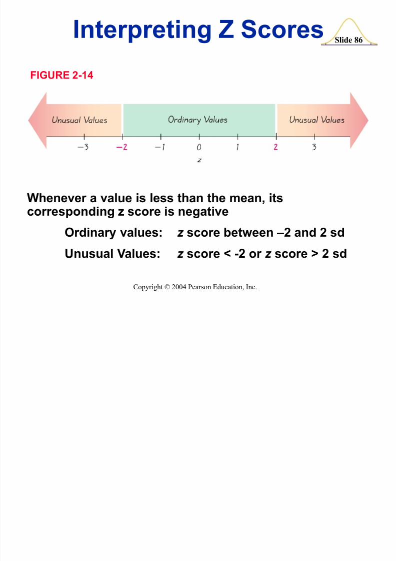
Interpreting Z Scores

Whenever a value is less than the mean, its

corresponding z score is negativeOrdinary values: z score between ±2 and 2 sd

U nusual Values: z score < -2 or z score > 2 sd

FIG U RE 2-14

8/7/2019 tes9e_ch02


Q til

8/7/2019 tes9e_ch02


Slide 88


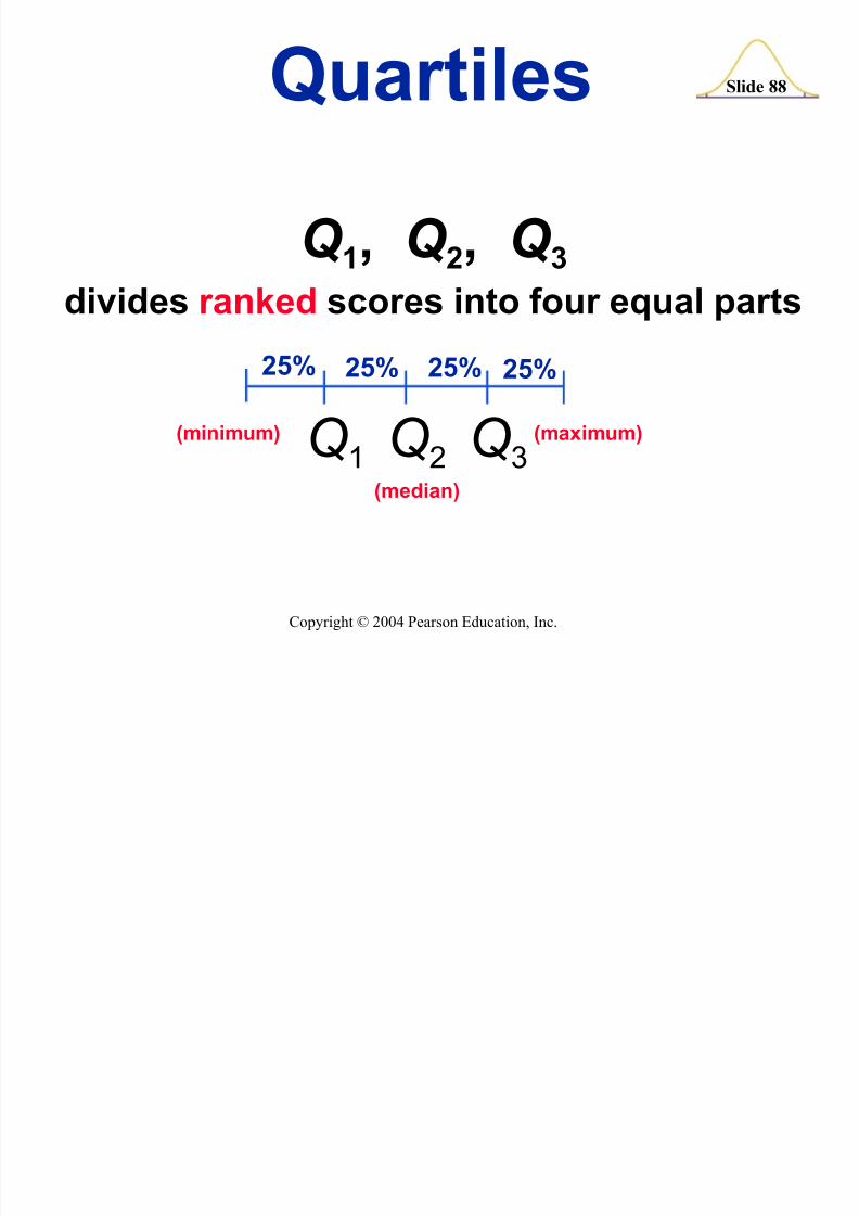
Q 1, Q 2, Q 3divides ranked scores into four equal parts

Quartiles

25% 25% 25% 25%

Q3

Q2

Q1

(minimum) (maximum)

(median)

Percentiles

8/7/2019 tes9e_ch02


Slide 89


Percentiles

Just as there are quartiles separating data

into four parts, there are 99 percentilesdenoted P 1, P 2, . . . P 99 , which partition thedata into 100 groups.

Finding the Percentile

8/7/2019 tes9e_ch02


Slide 90


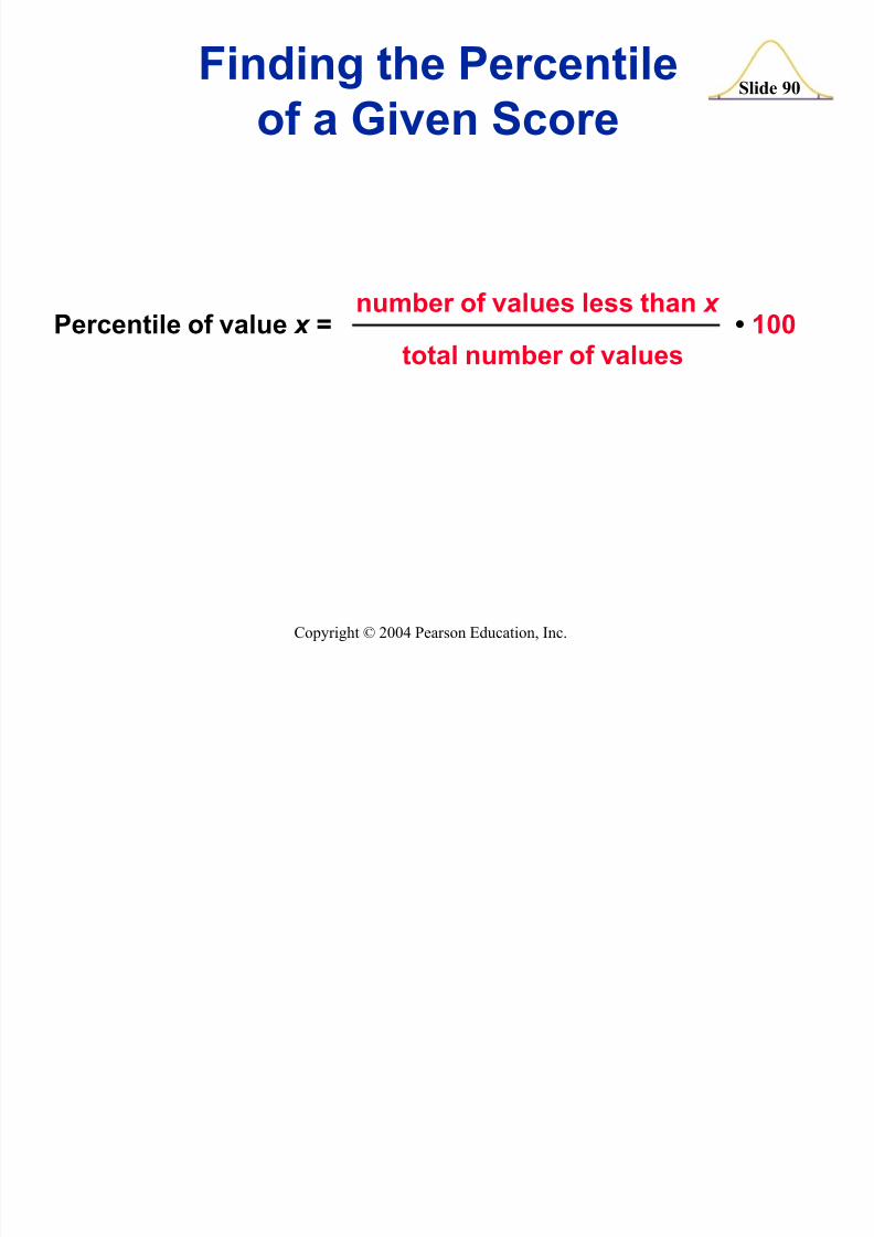
Finding the Percentileof a Given Score

Percentile of value x = 100number of values less than x

total number of values

Converting from the

8/7/2019 tes9e_ch02


Slide 91


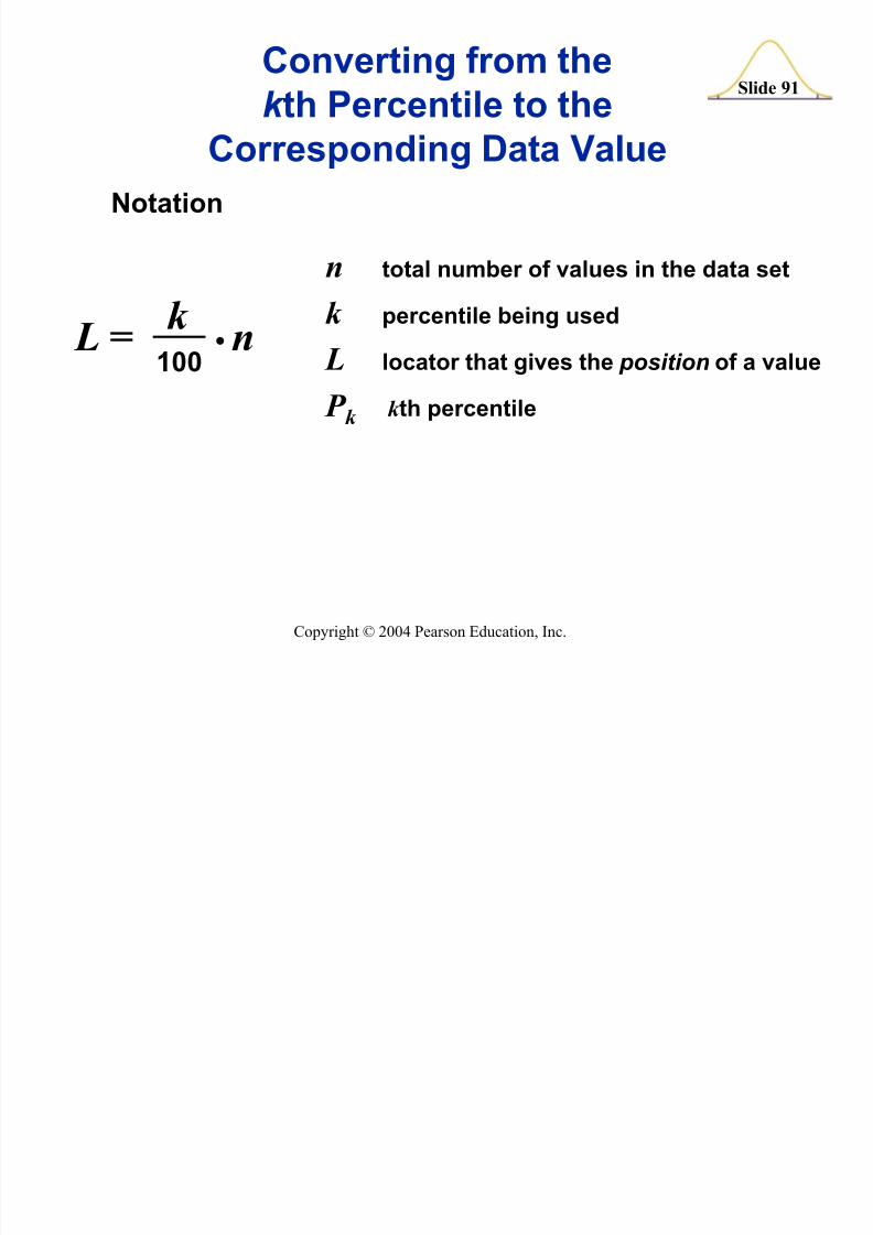
n total number of values in the data set

k percentile being used L locator that gives the position of a value

P k k th percentile

L = nk 100

N otation

Converting from thek th Percentile to the

CorrespondingD

ata Value

Converting

8/7/2019 tes9e_ch02


Slide 92


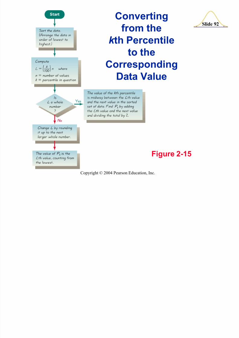
Figure 2-15

gfrom the

k th Percentileto the

CorrespondingD ata Value

Some Other Statistics

8/7/2019 tes9e_ch02


Slide 93


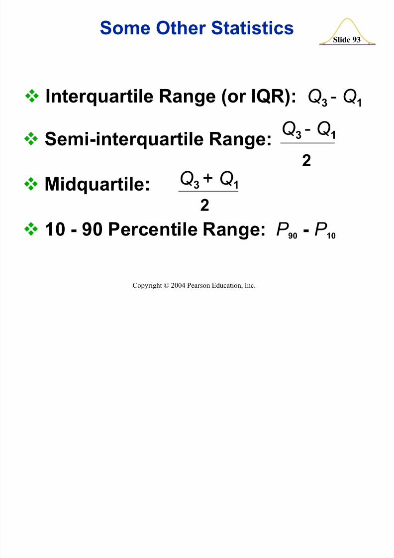
Interquartile Range (or IQR): Q 3 - Q 1

10 - 90 Percentile Range: P 90 - P 10

Semi-interquartile Range: 2

Q 3 - Q 1

Midquartile:

2

Q 3 + Q 1

Some Other Statistics

Recap

8/7/2019 tes9e_ch02


Slide 94


Recap

In this section we have discussed:

z Scores

z Scores and unusual values

Quartiles

Percentiles

Converting a percentile to corresponding datavalues

Other statistics

8/7/2019 tes9e_ch02


Slide 95



Section 2-7Exploratory D ata Analysis

(E D A)

D efinition

8/7/2019 tes9e_ch02


Slide 96


Exploratory D ata Analysis is theprocess of using statistical tools (such

as graphs, measures of center, andmeasures of variation) to investigatedata sets in order to understand their important characteristics

D efinition

D efinition

8/7/2019 tes9e_ch02


Slide 97


D efinition

An outlier is a value that is located veryfar away from almost all the other

values

Important Principles

8/7/2019 tes9e_ch02


Slide 98


Important Principles

An outlier can have a dramatic effect on themean

An outlier have a dramatic effect on thestandard deviation

An outlier can have a dramatic effect on thescale of the histogram so that the truenature of the distribution is totallyobscured

D efinitions

8/7/2019 tes9e_ch02


Slide 99


For a set of data, the 5-number summary consistsof the minimum value; the first quartile Q 1; themedian (or second quartile Q 2); the third quartile,

Q 3; and the maximum value

A boxplot ( or box-and-whisker-diagram ) is agraph of a data set that consists of a lineextending from the minimum value to themaximum value, and a box with lines drawn at thefirst quartile, Q 1; the median; and the thirdquartile, Q 3

D efinitions

Boxplots

8/7/2019 tes9e_ch02


Slide 100


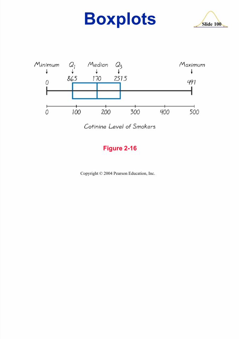
Boxplots

Figure 2-16

Boxplots

8/7/2019 tes9e_ch02


Slide 101


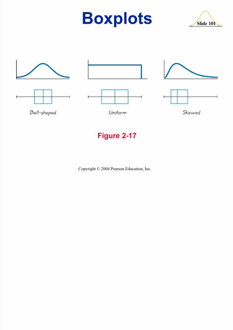
Figure 2-17

Boxplots

Slid 102Recap

8/7/2019 tes9e_ch02


Slide 102Recap

In this section we have looked at:

Exploratory D ata Analysis

Effects of outliers

5-number summary and boxplots

Documents

tes9e_ch02