Embed Size (px)
Citation preview

ARTICLE IN PRESS
Journal of Financial Economics 79 (2006) 507–536
0304-405X/$
doi:10.1016/j
$I thank
anonymous r�Tel.: +1
E-mail ad
www.elsevier.com/locate/jfec
Term structure estimation without usinglatent factors$
Gregory R. Duffee�
Haas School of Business, University of California, Berkeley, Berkeley, CA 94720, USA
Received 29 April 2004; received in revised form 4 January 2005; accepted 22 March 2005
Available online 10 October 2005
Abstract
A combination of observed and unobserved (latent) factors capture term structure dynamics.
Information about these dynamics is extracted from observed factors using restrictions implied by
no-arbitrage, without specifying or estimating any of the parameters associated with latent factors.
Estimation is equivalent to fitting the moment conditions of a set of regressions, where no-arbitrage
imposes cross-equation restrictions on the coefficients. The methodology is applied to the dynamics
of inflation and yields. Outside of the disinflationary period of 1979 through 1983, short-term rates
move one-for-one with expected inflation, while bond risk premia are insensitive to inflation.
r 2005 Elsevier B.V. All rights reserved.
JEL classification: C51; E43; E44
Keywords: Term structure; Dynamic models; Bond pricing
1. Introduction
Beginning with Vasicek (1977) and Cox et al. (1985), researchers have built increasinglysophisticated no-arbitrage models of the term structure. These models specify the evolutionof state variables under both the physical and equivalent martingale measures, and thuscompletely describe the dynamic behavior of yields at all maturities. Much of this researchfocuses on latent factor settings, in which the state variables are not directly observed by
- see front matter r 2005 Elsevier B.V. All rights reserved.
.jfineco.2005.03.007
Qiang Dai, George Pennacchi, Richard Stanton, seminar participants at many universities, an
eferee, and discussants Francis Longstaff and Ken Singleton for helpful comments.
510 642 1435; fax: +1 510 643 1420.
dress: [email protected].
ARTICLE IN PRESSG.R. Duffee / Journal of Financial Economics 79 (2006) 507–536508
the econometrician. Effectively, the evolution of yields is described in terms of yieldsthemselves. The important work of Piazzesi (2005) and Ang and Piazzesi (2003) broadensthis rather introspective view by including macroeconomic variables in the workhorseaffine framework of Duffie and Kan (1996). This extension allows us to investigatequestions at the boundaries of macroeconomics and finance. For example, what is theinformation in the output gap about the compensation that investors demand to take oninterest rate risk? What does today’s inflation rate say about the components of theexpected real returns of nominal long-term bonds? Intensive research focuses on these andrelated questions using models that describe the entire term structure with a combinationof macroeconomic and latent factors.1
Yet many of these questions can be examined without attempting to estimate thecomplete dynamics of the term structure. In a general asset pricing setting, Hansen andSingleton (1982) show that restrictions implied by no-arbitrage can be exploited withoutusing (or knowing) the complete joint dynamics of asset prices and the pricing kernel. It iseasy to adapt this idea to a term structure setting because a zero-coupon bond’s price issimply the expected value of the pricing kernel at the bond’s maturity. By conditioning thisexpectation on a set of macroeconomic variables, combining it with the conditionaldynamics of the same variables, and adding a couple of assumptions about riskcompensation, the relation between bond prices and the macroeconomic variables can bedetermined without specifying the remainder of the term structure.This paper explains how to project the term structure onto a set of observed factors and
thereby extract information from the factors about the future evolution of the termstructure. I refer to this projection as partial term structure estimation. The remainingvariation in the term structure is driven by latent factors, but latent factors play no role ineither parameter estimation or statistical tests of the model’s adequacy.Partial term structure estimation has two advantages over complete term structure
estimation. First, estimation is simplified substantially because researchers avoid specifyingfeatures of term structure dynamics that are not of direct interest. Second, misspecificationis less likely to contaminate estimates of the dynamics that are of interest. Forconcreteness, consider the relation between aggregate output and the term structure. Weknow that while output growth forecasts yields, yields also forecast output growth.Capturing these dynamics in a complete term structure model such as Ang et al. (2005)requires specifying both the number of latent factors and the functional forms for theirdynamics. For example, do latent factors follow moving average or autoregressiveprocesses? Are such factors Gaussian or do they exhibit stochastic volatility? Is theinformation in the latent factors about future output primarily information about near-term output growth (e.g., today’s one-quarter-ahead forecast of output depends on today’srealization of shocks to latent factors) or more distant output growth (e.g., today’s one-quarter-ahead forecast depends on lagged shocks to latent factors)?If our research goal is to model the complete term structure, we cannot avoid taking a
stand on its entire functional form. But if our goal is to use the information in the historyof output to forecast current and future bond yields and risk premia, latent factors arenuisance features of the model. The estimation procedure proposed here puts littlestructure on these factors. Neither the number of latent factors nor their functional
1Recent work includes Dewachter et al. (2002), Dewachter and Lyrio (2002), Hordahl et al. (2002), Ang and
Bekaert (2003), Ang et al. (2005), and Rudebusch and Wu (2003).

ARTICLE IN PRESSG.R. Duffee / Journal of Financial Economics 79 (2006) 507–536 509
relations with macro factors are specified. Intuitively, the procedure can be viewed as thejoint estimation of two sets of regressions. The first set consists of regressions of changes inbond yields on changes in the macro factors. These regressions are estimated withinstrumental variables, where the instruments are lagged macro factors. The second setrepresents the regressions comprising a vector autoregression for the macro factors. No-arbitrage imposes cross-equation restrictions on the parameters.
I use this estimation framework to study two questions concerning the relation betweeninflation and the nominal term structure. First, how sensitive are short-term interest rates toinflation? Second, how sensitive are bond risk premia to inflation? The empirical analysisfocuses on two periods, namely, the ‘‘pre-Volcker’’ period, from 1960 through the secondquarter of 1979, and the ‘‘post-disinflation’’ period, from 1984 through 2003. The evidenceindicates that during both periods, short-term rates move approximately one-for-one withchanges in expected inflation, where the expectations are conditioned on the history ofinflation. This result might appear to contradict the existing Taylor rule literature whichconcludes that the Federal Reserve (Fed) reacted more aggressively to inflation in thedisinflationary period than it did in the pre-Volcker period. However, the discrepancy islargely driven by the behavior of inflation and interest rates during 2002 and 2003.
Surprisingly, bond risk premia are fairly insensitive to inflation in both periods. Riskpremia are somewhat lower when inflation is high, but the contribution of inflation tovariation in risk premia is economically small. The relation is strongest in the early period,with the standard deviation of excess quarterly returns to a five-year bond conditioned oninflation at about 13 basis points. Put differently, the relation between changes in inflationand changes in the shape of the term structure is determined almost entirely by changes inexpected short rates, not by changes in risk premia.
The next section describes the modeling framework and the estimation methodology.Section 3 applies the methodology to the relation between inflation and the term structure.Section 4 concludes.
2. The model and estimation technique
Underlying the dynamics of bond yields is some structural model that explains thesedynamics in terms of the state of the macroeconomy, central bank policy, and thewillingness of investors to bear interest rate risk. Although the model here includesobservable variables, it is not a structural model. In particular, nothing here identifiesmonetary policy shocks. The model is closer in spirit to a reduced form model linking bondyields to macro variables. The formal structure is closely related to the model of Ang andPiazzesi (2003).
Time is indexed by discrete periods t, where length of a period is Z years. There are n0
observable variables realized at time t and stacked in a vector f 0t . The natural application
of the model is to macroeconomic variables such as inflation and output. In principle,however, this vector can include any observed variable that we are interested in relating tobond yields. Accordingly, I generally refer to f 0
t as a vector of observables rather than avector of macro variables.
The vector of observed factors f t used in the model contains lags zero through p� 1of f 0
t :
f t � ðf00
t f 00
t�1 . . . f 00
t�ðp�1ÞÞ0. (1)

ARTICLE IN PRESSG.R. Duffee / Journal of Financial Economics 79 (2006) 507–536510
The length of f t is nf ¼ pn0. While the choice of p is discussed at various places inthis section, for the moment it is sufficient to note that lags are important both informing forecasts of future realizations of f 0
t and in capturing variations in short-term interest rates that are not associated with f 0
t . In a term structure setting it is importantto distinguish between contemporaneous variables f 0
t and the entire state vector f t.Bond prices depend on compensation that investors require to face one-step-ahead uncertainty in the state vector. In (1), only f 0
t is stochastic given investors’information at t� 1.The period-t price of a bond that pays a dollar at period tþ t is Pt;t. The continuously
compounded annualized yield is yt;t. The short-term interest rate, which is equivalent tothe yield on a one-period bond, is rt. Observed factors are related to the term structure, butthey are insufficient to explain the complete dynamics of the term structure; latent factorspick up all other variation in bond yields. There are nx latent factors stacked in a vector xt.The relation between the factors and the short rate is affine:
rt ¼ d0 þ d0f f t þ d0xxt. (2)
Bond prices satisfy the law of one price,
Pt;t ¼ EtðMtþ1Ptþ1;t�1Þ, (3)
where Mtþ1 is the pricing kernel. The term structure of bond yields depends on the jointdynamics of the pricing kernel, the observed factors, and the latent factors. To motivatethe method for estimating the relation between observed factors and the term structure, itis easiest to start with the special case in which the observed factors are independent of thelatent factors. The estimation technique in the more general case of correlated factors onlyrequires a slight (but vital) modification to the method that is appropriate forindependence.
2.1. Independence between observed and latent factors
The contemporaneous observed variables f 0t are assumed to follow a vector
autoregressive process (VAR) with at most p lags. We can always embed a VAR withfewer than p lags into a VAR(p). Since the mathematics of affine term structure models areusually expressed in terms of first order dynamics, it is convenient to express the observeddynamics as a VAR(1) model for f t:
f tþ1 � f t ¼ mf � Kff f t þ Sf �f ;tþ1. (4)
The components on the right-hand side of (4) are
mf ¼m0
0ðnf�n0Þ�1
!; Kff ¼
K0
C
� �,
Sf ¼S0 0n0�ðnf�n0Þ
0ðnf�n0Þ�n0 0ðnf�n0Þ�ðnf�n0Þ
!; and �f ;tþ1 ¼
�0;tþ1
0ðnf�n0Þ�1
!. (5)
The vector m0 has length n0, the matrix K0 is n0 � nf , and the matrix S0 is n0 � n0. Theelements of the n0-length vector �0;tþ1 are independent standard normal innovations. The

ARTICLE IN PRESSG.R. Duffee / Journal of Financial Economics 79 (2006) 507–536 511
companion matrix C has the form
C ¼
�I I 0 . . . 0 0
. . .
0 0 0 . . . �I I
0B@
1CA. (6)
The square submatrices in C all have dimension n0. The double subscript on Kff is used forconsistency with the model of correlated factors presented in Section 2.3.
The dynamics of the latent factors have the general affine representation
xtþ1 � xt ¼ mx � Kxxxt þ SxSxt�x;tþ1, (7)
where Sxt is a diagonal matrix with elements
SxtðiiÞ ¼
ffiffiffiffiffiffiffiffiffiffiffiffiffiffiffiffiffiffiffiffiffiffiaxi þ b0xixt
q. (8)
The elements of �x;tþ1 are independent standard normal innovations. No additional detailabout latent factor dynamics is either necessary or useful.
The pricing kernel has the standard log-linear form
logMtþ1 ¼ �Zrt � L0ft�f ;tþ1 � L0xt�x;tþ1 � ð1=2ÞðL0ftLft þ L0xtLxtÞ. (9)
The vectors Lft and Lxt are the prices of �f ;tþ1 risk and �x;tþ1 risk, respectively. Since f 0tþ1 is
the only component of f tþ1 that is unknown at t, without loss of generality the former priceof risk can be expressed as
Lft ¼L0t
0ðnf�n0Þ�1
!. (10)
The n0-vector L0t is the price of risk associated with innovations to f 0tþ1. The price of
observed-factor risk, which is the product of observed-factor volatility and thecompensation required for exposure to �f ;tþ1, depends on observed and latent factors:
Sf Lft �S0L0t
0ðnf�n0Þ�1
!¼
lf þ ðlff lfxÞf t
xt
!
0ðnf�n0Þ�1
0BB@
1CCA. (11)
The vector lf has length n0, the matrix lff is n0 � nf , and the matrix lfx is n0 � nx. This isthe Gaussian special case of the essentially affine price of risk introduced in Duffee (2002).The price of risk associated with latent factor shocks has the similar form
SxSxtLxt ¼ lx þ ðlxf lxxÞf t
xt
!. (12)
Conditions under which this form satisfies no-arbitrage (in the continuous-time limit) arediscussed in Kimmel et al. (2004). As written, (12) allows the price of latent factor risk todepend on both observed and latent factors. This general functional form is tightened atthe end of this subsection through the introduction of a key restriction.
The recursion used to solve for bond prices in an affine setting is standard. Campbellet al. (1997) provide a textbook treatment. I nonetheless go through a few of the steps here

ARTICLE IN PRESSG.R. Duffee / Journal of Financial Economics 79 (2006) 507–536512
for future reference. Guess that log bond prices are affine in the factors, that is,
logPt;t ¼ At þ B0f ;t f t þ B0x;txt. (13)
The recursion implied by the law of one price (3), combined with the normally distributedshocks to f t and xt and the independence between f t and xt, produces
At þ B0f ;t f t þ B0x;txt ¼ � Zrt þ At�1
þ B0f ;t�1Etðf tþ1Þ þ B0x;t�1Etðxtþ1Þ
þ1
2B0f ;t�1Sf S0f B0f ;t�1 þ B0x;t�1SxS2
xtS0f B0x;t�1
� �
� B0f ;t�1
lf þ ðlff lfxÞf t
xt
!
0ðnf�n0Þ�1
0BB@
1CCA
� B0x;t�1 lx þ ðlxf lxxÞf t
xt
! !. ð14Þ
The factor loadings Bf ;t and Bx;t are determined by this recursion. Substitute into (14) theshort-rate equation (2) and the conditional expectation of f tþ1 from (4), then matchcoefficients in f t. The result is the difference equation
B0f ;t ¼ �Zd0f þ B0f ;t�1ðI � K
qff Þ � B0x;t�1lxf . (15)
The matrix Kqff in (15) is the counterpart to Kff under the equivalent martingale measure,
and is given by
Kqff ¼
K0 þ lff
C
� �. (16)
Matching coefficients in xt produces another difference equation that, combined with (15),allows for the joint calculation of the loadings Bf ;t and Bx;t. Yet another differenceequation produces the constant terms At. These other recursions are not relevant here.The combination of the observed factor dynamics (4), the latent factor dynamics (7), and
the coefficients of log bond prices in (13) completely characterize the behavior of bondprices. For example, both the unconditional expectation of logPt;t and its expectationconditioned on time t� 1 factor values can be calculated. This characterization allowsestimation of the model’s parameters using the dynamics of observed factors and bondyields. To date, researchers using no-arbitrage models to study term structure dynamicshave estimated these complete term structure models. In other words, each parameter’svalue is either fixed by the researcher or estimated. The motivation behind thismethodology is simple: our ultimate goal is to understand all of the dynamic patterns inthe term structure.An alternative path to this goal requires less ambitious modeling efforts. Instead of
estimating all of the parameters of a term structure model that is unavoidably misspecified,particular components can be estimated while leaving the remainder unspecified. This isthe point of the estimation procedure described in the next subsection. The relationbetween observed factors and the term structure is estimated without characterizing thepart of the term structure that is unrelated to the observed factors. No parameters

ARTICLE IN PRESSG.R. Duffee / Journal of Financial Economics 79 (2006) 507–536 513
associated with latent factors are estimated. In fact, not even the number of latent factors isspecified.
An additional assumption is necessary. The price of risk of innovations in the latentfactors is assumed to not depend on the level of the observed factors. Formally, the generalform of the price of risk in (12) is restricted by
lxf ¼ 0. (17)
The role of this assumption is highlighted in the next subsection.
2.2. Partial term structure estimation with independent factors
The parameters that are identified and estimated by this procedure are df in (2), m0 andK0 in (5), and lff in (11). There are three key results that guide the econometricmethodology. The first is that the observed factor loadings Bf ;t depend only on theseparameters and not on any parameters associated with the latent factors. With assumption(17), the loading on the latent factors drops out of (15). We can then solve explicitly theresulting recursion for observed factor loadings without reference to the parameters of thelatent factor dynamics. The solution is
Bf ;t ¼ �ðKqff
0Þ�1ðI � ðI � K
qff
0ÞtÞZdf . (18)
Given K0, lff , and the matrix of constants C defined in (6), the matrix Kqff is determined by
(16). Therefore the factor loadings in (18) can be computed.The second key result is that the expectation of differenced log bond yields conditioned
on observed variables depends only on information about the observed variables. Tounderstand this result, first-difference the general bond pricing equation (13), divide by thenegative of the bond’s maturity (in years) Zt to express it in terms of annualized yields, andrearrange terms, denoting first differences with D:
Dyt;t ��B0f ;t
Zt
� �Df t ¼
�B0x;tZt
� �Dxt. (19)
The purpose of the first differencing is to remove both At and the unconditional mean ofthe latent factors. Next, remove any other information about the latent factors by takingthe expectation of (19) conditioned on Df t. Because f t and xt are independent, theconditional expectation of the right side of (19) is zero, that is,
E Dyt;t ��B0f ;t
Zt
� �Df t
����Df t
� �¼ 0. (20)
Note that the conditional expectation depends only on Bf ;t and Df t.The third key result is that conditional expectations of the observed factors identify the
physical dynamics of f t, and thus identify the parameters of these dynamics. From (4), theexpectation of Df t conditioned on f t�1 is
EðDf tjf t�1Þ � ðmf � Kff f t�1Þ ¼ 0. (21)
The parameters that link the observed factors to bond yields can be estimated withgeneralized method of moments (GMM) using the bond pricing formula (18) and themoment conditions (20) and (21). At each date t ¼ 1; . . . ;T we observe the contempora-neous observed factors f 0
t and the yields yt;tiof L zero-coupon bonds with maturities t1

ARTICLE IN PRESSG.R. Duffee / Journal of Financial Economics 79 (2006) 507–536514
through tL. Denote a candidate parameter vector as
F ¼ ðm0 d0f vecðK0Þ0 vecðlff Þ
0Þ0. (22)
There are n0 þ nf þ 2n0nf parameters in F; n0 in m0, nf in df , and n0nf in both of K0 andlff . Denote the true parameter vector by F0.Given a parameter vector, the implied observed factor loadings Bf ;t1 through Bf ;tL
canbe calculated with (18). The moment vector for observation t is
htðFÞ ¼
Dyt;t1 ��B0
f ;t1Zt1
� �Df t
� �� Df t
� � �
Dyt;tL�
�B0f ;tL
ZtL
� �Df t
� �� Df t
ðDf 0t � m0 þ K0f t�1Þ �
1
f t�1
!
0BBBBBBBBB@
1CCCCCCCCCA. (23)
The unconditional expectation of ht is zero when it is evaluated at F0.We can think of these moments as the moments associated with Lþ n0 ordinary least
squares (OLS) regressions, modified by the requirement of no-arbitrage. To make thisclear, consider the top expression in the moment vector, which represents nf momentsassociated with the t1-maturity bond. If no-arbitrage is not imposed, the vector Bf ;t1 isunrestricted and this set of moments corresponds to the moments of the OLS regression ofdifferenced bond yields on differenced observed factors. (There is no constant term in theregression.) Without the requirement of no-arbitrage, the estimate of �Bf ;t1=ðZt1Þ equalsthe coefficients produced by this regression. Similar OLS regressions are estimated for eachof the L bonds. By imposing no-arbitrage, the coefficients from these regressions arerequired to satisfy cross-equation restrictions.Now consider the bottom expression in the moment vector, which represents n0 � ð1þ
nf Þ moments. If no-arbitrage is not imposed, this expression corresponds to the momentsof n0 OLS regressions of the VAR(p) model of the observed factors. The estimate of K0 isthen determined by the VAR parameter estimates. If no-arbitrage is imposed but thefeedback matrix K0 under the physical measure has no parameters in common with thefeedback matrix K0 þ lff under the equivalent martingale measure, the interpretation ofthese moments is unchanged. If any parameter restrictions are placed on lff , cross-equation restrictions link the observed factor dynamics and the bond price dynamics.The parameter estimates solve
F� ¼ argmaxF
gT ðFÞ0WgT ðFÞ, (24)
where gT is the mean moment vector
gT ðFÞ ¼XT
t¼1
htðFÞ (25)
and W is some weighting matrix. The moment vector has length Lnf þ n0ð1þ nf Þ. If norestrictions are placed on the model’s parameters, the number of moments less the numberof free parameters is nf ðL� 1� n0Þ. Thus all of the parameters are exactly identified whenthe number of bonds L is one greater than the number of variables in the contemporaneous

ARTICLE IN PRESSG.R. Duffee / Journal of Financial Economics 79 (2006) 507–536 515
observed vector f 0t . Including additional bonds produces overidentifying restrictions that
can be used to test the adequacy of the model.
2.3. Dependence between observed and latent factors
A large literature documents that the term structure contains information about futurerealizations of some macro variables, such as output and inflation, that is not contained inthe history of these macro variables.2 Thus, for at least some choices of observed variables,the assumption of independence between observed and latent factors is untenable. Thissubsection generalizes the model to allow for correlations between observed and latentfactors. Conveniently, the partial term structure estimation technique described in Section2.2 requires little modification in order to incorporate the correlation structure introducedhere. The formal modeling framework is presented below, and is followed by an example.
2.3.1. The model
The following dependence is allowed between the observed and latent factors:
Eðf tjxt�jÞ unrestricted; j40; (26)
Eðxtjf t�jÞ ¼ 0; jX0. (27)
Eq. (26) allows the latent factors to forecast future observed factors, while (27) says thatobserved factors have no forecasting power for current or future latent factors. Thissecond equation is less restrictive than it appears. In part, it imposes a normalization onthe decomposition of the short rate into pieces related to observable and latent factors. Theexample of Section 2.3.2 illustrates the restrictions and normalizations built into (27).
The dynamics of the latent factors are given by (7), which are the same dynamics used inthe case of independence. The dynamics of observed factors are
f tþ1 � f t ¼ mf � Kff f t � Kfxxt þ Sf �f ;tþ1. (28)
Consider the ‘‘own’’ dynamics of observed factors, that is, the dynamics conditioned onlyon the history of the observed factors. From (28) and (27), these dynamics are
f tþ1 � f t ¼ mf � Kff f t þ xtþ1, (29)
xtþ1 ¼ �Kfxxt þ Sf �f ;tþ1; Eðxtþ1jf t; . . . ; f t�1Þ ¼ 0. (30)
In words, the own dynamics for f t are an AR(1) (with, perhaps, stochastic volatilityintroduced by xt), or equivalently, the own dynamics for f 0
t are an AR(p).The joint dynamics of the observed factors (28) and latent factors (7) must satisfy (27).
The fact that f t does not appear in (7) does not guarantee that (27) holds. The Appendixdescribes parameter restrictions on Kfx and the latent factor dynamics (7) that aresufficient to imply (27). Because Kfx and all of the components of (7) drop out of theestimation procedure, these restrictions do not need to be imposed explicitly in theestimation.
2The literature is too large (and only indirectly related to this paper) to cite fully. See Ang et al. (2005) and
Diebold et al. (2003) for discussions of this forecastability and references to the relevant literature.

ARTICLE IN PRESSG.R. Duffee / Journal of Financial Economics 79 (2006) 507–536516
The model is completed with the dynamics of the pricing kernel in (9), which are thesame dynamics used for the case of independent factors. The functional forms for riskcompensation are (11) and (12), which also carry over from the case of independence.Bond pricing formulas are calculated in the usual way. Guess the log-linear form (13)
holds and apply the law of one price. The result is (14). Although the form of this equationis unchanged by the introduction of correlated factors, the interpretation is different. Withcorrelated factors, the period-t expectation of f tþ1 depends on both observed and latentfactors. As in the case of independent factors, match coefficients from (14) in f t. This stepuses the special structure placed on the joint dynamics of f t and xt. Because Etðxtþ1Þ doesnot depend on f t, this matching results in the recursion (15), as in the case of independentfactors. Finally, by imposing assumption (17), the recursion for Bf ;t can be solvedexplicitly, producing (18), as in the case of independence.Why are the observed factor loadings Bf ;t unchanged when the assumption of
independence between observed and latent factors is dropped? The reason relates to therestrictions imposed by (27). Because the latent factors are associated with future observedfactors but not current or past observed factors, the projection of the term structure ontoobserved factors is unaffected by the latent factors. The projection throws awayinformation in the term structure about the future evolution of the observed factors, butthis information does not affect the sensitivity of yields to f t. Thus, the only implicationof introducing correlated factors is that the model’s parameters can no longer be estimatedwith the technique described in Section 2.2. A modified technique is described inSection 2.4.
2.3.2. An example
The short rate is determined by contemporaneous inflation and the contemporaneousoutput gap,
rt ¼ d0 þ pt þ gt, (31)
where pt is inflation and gt is a measure of the output gap. (For simplicity, the coefficientsin this Taylor rule equation are both one.) The dynamics of output and inflation are
gt ¼ cg þ yg;p;0pt þ yg;p;1pt�1 þ zt þ �g;t, (32)
zt ¼ yzzt�1 þ �z;t, (33)
and
pt ¼ cp þ yppt�1 þ c�g;t�1 þ �p;t. (34)
The shocks �g;t, �z;t, and �p;t are normally distributed and are independent at all leads andlags. The coefficient yg;p;0 picks up any contemporaneous relation between shocks toinflation and output. Inflation also leads output through yg;p;1. Output has a component zt
that is independent of inflation at all leads and lags, and a component �g;t that leadsinflation.An econometrician wants to investigate the relation between inflation and the term
structure without using information about output. Thus from the econometrician’sperspective, the short rate is driven by observed inflation and latent factors. There are avariety of ways to express the short rate as the sum of observed and latent factors. Oneobvious expression is simply (31) where f t ¼ pt and xt ¼ gt. But without information

ARTICLE IN PRESSG.R. Duffee / Journal of Financial Economics 79 (2006) 507–536 517
about output, it is impossible to distinguish the direct link between inflation and the shortrate from the indirect link associated with the contemporaneous covariance betweeninflation and output. The natural restriction is to impose a zero covariance between f t andxt. Indeed, it is imposed by (27) with j ¼ 0. With this restriction and the choice of f t ¼ pt,xt is the residual from a regression of gt on pt.
However, this decomposition does not satisfy all of the restrictions built into (27). Whenf t ¼ pt, there are two channels through which f t forecasts future short rates. First, currentinflation forecasts future inflation (and therefore future f t) through (34). Second, currentinflation forecasts future output (and therefore future xt) through (32). The second channelviolates (27) for j40.
To satisfy (27), the vector of observed factors must be expanded to include laggedinflation. The appropriate decomposition of rt into observed and latent factors is
f t ¼pt
pt�1
!; xt ¼
zt
�g;t
!, (35)
df ¼1þ yg;p;0
yg;p;1
!; dx ¼
1
1
� �. (36)
With the definitions of f t and xt in (35), verification of (27) is straightforward. The secondelement of xt is correlated with ptþj ; j40, while xt is independent of pt�j ; jX0.
The econometrician cannot rely on the structure of the model to produce thisdecomposition because, by assumption, no data on output are available to determine thedynamics in (32). The appropriate rule to follow is that the vector f t must include all lagsof pt that have independent information about the short rate. Put somewhat differently,the choice of lag length p maximizes the explanatory power of f t for the short rate. Sincethe econometrician does not know the true data generating process of rt, a reasonableapproach is to choose a lag length and then test its adequacy by checking whetheradditional lags help to forecast the short rate. Section 3.2 contains an application of thisprocedure.
Although f t requires only one additional lag of inflation in this example, alternative datagenerating processes can require a large number of lags. To take an extreme example,replace the dynamics of output and inflation above with the bivariate VAR
pt
gt
!¼ y
pt�1
gt�1
!þ S
�1;t
�2;t
!, (37)
where the elements of y and S are arbitrary. If gt is not observed, every lag pt�j containssome independent information about the evolution of rt. Therefore, unless f t contains aninfinite number of lags, (27) is technically violated. But in practice, the amount ofindependent information in distant lags might be too small to distinguish from samplingerror.
Model estimation in the presence of correlated factors is discussed in the nextsubsection. Before getting into the details, it is worth noting the consequences of using avector of observed factors f t that does not satisfy the conditional expectation requirement(27). In the context of the example here, assume the econometrician uses f t ¼ pt instead off t ¼ ðpt pt�1Þ
0. This choice of f t produces a misspecified loading Bf ;t on pt. The problem

ARTICLE IN PRESSG.R. Duffee / Journal of Financial Economics 79 (2006) 507–536518
arises in the matching of coefficients on f t in (14). Because (27) is violated, the trueconditional expectation Etðxtþ1Þ depends on pt. Therefore Bf ;t depends on Bx;t�1, but thisdependence is ignored in calculating Bf ;t. Hence, not only is the econometrician throwingaway information in pt�1 that would help forecast the term structure—the information inpt is also used incorrectly.
2.4. Partial term structure estimation with correlated factors
As in the case of independence, here the parameters df , m0, K0, and lff can be estimatedwithout imposing additional structure on the latent factors. However, there is oneimportant difference. With independence, the expectation of the right-hand side of (19)conditioned on Df t is zero. With correlated factors, this is no longer true because xt�1 maycontain information about f t. Instead, take the expectation of (19) conditioned on f t�1 andapply (27):
E Dyt;t ��B0f ;t
ZtDf t
� ����f t�1
�¼ 0. (38)
The corresponding moment vector for observation t is
htðFÞ ¼
Dyt;t1 ��B0
f ;t1Zt Df t
� � �
Dyt;tL��B0
f ;tL
Zt Df t
Df 0t � m0 þ K0f t�1
0BBBBB@
1CCCCCA�
1
f t�1
!. (39)
Recall that with independence between observed and latent factors, the moment vector(23) is interpreted as moments of OLS regressions in which cross-equation restrictions areimposed on the OLS parameter estimates. Almost the same interpretation can be appliedto (39). The only difference is that the regressions of differenced yields on differencedobserved factors are estimated with instrumental variables instead of OLS.The instruments are a constant and lagged observed factors. As with (23), no-arbitrage imposes cross-equation restrictions on the estimated parameters. Section 3contains some additional discussion about the inappropriateness of OLS momentconditions when the latent factors contain information about future realizations of theobserved factors.This estimation procedure can use yields on bonds of any maturity. In particular, it is
not necessary to observe the short rate. However, if the short rate is observed, a singleinstrumental variable (IV) regression can be used to estimate the short-rate loadings df .Denote the instruments used in the moment condition (39) as z0t�1 ¼ f1 f 0t�1g. Write thechange in the short rate from t� 1 to t as the sum of two pieces, in particular, a componentthat is projected on zt�1 and a residual. The result is
Drt ¼ d0f ðEðDf tjzt�1ÞÞ þ fd0f ð�Kfxxt þ Sf �f ;tÞ þ d0xDxtg, (40)
where
EðDf tjzt�1Þ ¼ mf � Kff f t�1. (41)

ARTICLE IN PRESSG.R. Duffee / Journal of Financial Economics 79 (2006) 507–536 519
The residual term in curly brackets is orthogonal to f t�1. Thus a regression of changes inthe short rate on changes in the observed factors using instruments zt�1 produces aconsistent estimate of df .
The remainder of this section examines in detail some of the features of this model. Thenext subsection discusses the role played by the affine structure of the latent factors.
2.5. Relaxing the affine structure
The affine dynamics of the latent factors xt are not essential. The affine form guaranteesconditional joint log-normality of bond prices and the pricing kernel, which in turnproduces the recursion (14) from the law of one price. This subsection describes analternative framework that allows for nonlinear dynamics, where conditional joint log-normality is simply assumed. This framework leads to the identical estimation proceduredescribed in the previous subsection.
Replace the observed factor dynamics (28) with
f tþ1 � f t ¼ mf þ Kff f t þ KfxðxtÞ þ Sf �f ;tþ1, (42)
where KfxðxtÞ is an unspecified function of the latent factors that can be nonlinear. Replacethe latent factor dynamics (7) with
xtþ1 � xt ¼ KxxðxtÞ þ SxSxðxtÞ�x;tþ1, (43)
where KxxðxtÞ and SxðxtÞ are also unspecified functions of the latent factors that can benonlinear. The innovations �f ;tþ1 and �x;tþ1 are multivariate standard normal shocks thatare independent at all leads and lags. Therefore, shocks to both types of factors areconditionally normal. Independence between shocks to observed and latent factors isconsistent with the normalization that latent factors contain information about futurerealizations of observed factors, but not information about current or past realizations.Both types of shocks appear in the stochastic discount factor, which is the same function(9) used in the affine model.
Replace the affine form for log bond prices (13) with
logPt;t ¼ At þ B0f ;t f t þ wtðxtÞ, (44)
where wtðxtÞ is a (perhaps nonlinear) function of xt with conditionally normal shocks:
wtðxtþ1Þ ¼ Etðwtðxtþ1ÞÞ þ et;tþ1; et;tþ1�Nð0;Vartðet;tþ1ÞÞ. (45)
As with the shocks to the latent factors, the shocks to these functions of latent factors arealso independent of the shocks to observed factors �f ;tþ1. Eq. (44), with t ¼ 1, replaces theshort-rate equation (2).
While the functional form of wðtÞ is unspecified here, it is not arbitrary. No-arbitragerestricts the form of wðtÞ given the form of wðt� 1Þ. Here I simply assume that there is asequence of functions wð1Þ;wð2Þ; . . ., such that no-arbitrage is satisfied.
With these assumptions, the law of one price (3) implies
At þ B0f ;t f t þ wtðxtÞ ¼ A1 þ B0f ;1 f t þ w1ðxtÞ þ At�1
þ B0f ;t�1Etðf tþ1Þ þ Etðwt�1ðxtþ1ÞÞ

ARTICLE IN PRESSG.R. Duffee / Journal of Financial Economics 79 (2006) 507–536520
þ 12ðB0f ;t�1Sf S0f Bf ;t�1 þ Vartðet�1;tþ1ÞÞ
� B0f ;t�1Sf Lft � Covtðet�1;tþ1;L0xt�x;tþ1Þ. ð46Þ
As with the affine model, the next step is to take the expectation of (46) conditioned on f t.A few additional assumptions are necessary for the terms involving the latent factors todrop out of this conditional expectation. The first two assumptions replace the restriction(27). First, the component of the expectation of f tþ1 that is related to the latent factors hasan expectation of zero when conditioned on f t:
EðKfxðxtÞjf tÞ ¼ 0. (47)
Second, the expectation of wðtÞ conditioned on both f t and f t�1 is zero for all t:
EðwðtÞjf t; f t�1Þ ¼ 0 8t. (48)
Third, the variance of et;tþ1 conditioned on f t is constant:
EðVartðet;tþ1Þjf tÞ ¼ V t. (49)
Fourth, the conditional expectation of the compensation for facing observed-factor risk is
Sf EðLftjf tÞ ¼lf þ lff f t
0ðnf�n0Þ�1
!. (50)
Finally, the restriction on the dynamics of latent-factor risk premia given in (17) is replacedwith
EðCovtðet�1;tþ1;L0xt�x;tþ1Þjf tÞ ¼ Ct�1. (51)
The expectation of (46) conditioned on f t is therefore
B0f ;tf t ¼ kt þ B0f ;1f t þ B0f ;t�1ðI � Kff � lff Þf t, (52)
where kt is a maturity-dependent constant. Matching coefficients in f t produces the bondpricing formula (18) with Zdf ¼ �Bf ;1. The own dynamics of f t are a VAR(1). Thus, themodel’s implications are identical to those of the affine model with correlated factors.
2.6. Applications
This subsection illustrates the kinds of questions that can be addressed with the partialterm structure estimation methodology.
�
How does the expected time path of rt vary with f t?The expected change in the short rate from t to tþ j, conditioned on f t, is
Eðrtþj � rtjf tÞ ¼ d0f ðI � ðI � Kff ÞjÞðK�1ff mf � f tÞ. (53)
Note that this j-ahead forecast is not a minimum variance forecast. There is additionalinformation in the term structure (such as the current level of the short rate) that is ignoredin forming this conditional expectation. Therefore, the partial term structure dynamicsshould not be used to forecast, but rather to interpret the link between the observed factorsand the term structure.
ARTICLE IN PRESSG.R. Duffee / Journal of Financial Economics 79 (2006) 507–536 521
�
How do risk premia on bonds vary with f t?The partial nature of the estimated model does not pin down mean excess bond returns.However, it does determine how variations in f t correspond to variations in expectedexcess returns. The expected excess log return to a t-maturity bond held from t to tþ 1,conditioned on f t, is
EðlogPtþ1;t�1 � logPt;t � Zrtjf tÞ ¼ kt þ B0f ;t�1
lff
0ðnf�n0Þ�nf
!f t. (54)
The constant term kt is unrestricted.
�
What is the shape of the term structure conditioned on f t?The expectation of the t-maturity annualized bond yield yt;t, conditioned on f t, is
Eðyt;tjf tÞ ¼ at þ1
td0f ðI � ðI � K
qff Þ
tÞðK
qff Þ�1f t. (55)
The constant term at is unrestricted.
�
What is the expected evolution of the term structure conditioned on f t?The j-period-ahead forecast of the change in the yield on a bond with constant maturityt is
Eðytþj;t � yt;tjf tÞ ¼1
td0f ðI � ðI � K
qff Þ
tÞðK
qff Þ�1ðI � ðI � Kff Þ
jÞ
�ðK�1ff mf � f tÞ. ð56Þ
�
Is the empirical failure of the expectations hypothesis associated with f t?Campbell and Shiller (1991) estimate regressions of the form
ytþs;l�s � yt;l ¼ b0 þ b1s
l � sðyt;l � yt;sÞ þ etþs;l;s (57)
for maturities l4s. Under the weak form of the expectations hypothesis the coefficient b1
should equal one, but in the data it is often negative. A common interpretation of thisresult is that bond risk premia and the slope of the term structure are positively correlated.The results of partial term structure estimation can be used to determine if the failure ofthe expectations hypothesis is seen in the part of the term structure that is associated withf t. Consider estimating (57) using f t as instruments. If the data are generated by the affinemodel described in this section, the conditional expectation of yield spread on the right-hand side of (57) is
Eðyt;l � yt;sjf tÞ ¼ yl;s þ �1
lBf ;l þ
1
sBf ;s
� �0f t, (58)

ARTICLE IN PRESSG.R. Duffee / Journal of Financial Economics 79 (2006) 507–536522
where yl;s is an unrestricted constant. The conditional expectation of the left-hand sideof (57) is
Eðytþs;l�s � yt;l jf tÞ ¼ fl;s þs
l � sEðyt;l � yt;sjf tÞ
�1
l � sB0f ;l�sððI � Kff Þ
s� ðI � K
qff Þ
sÞf t, ð59Þ
where fl;s is an unrestricted constant. If lff ¼ 0, then Kff ¼ Kqff and the final term in (59) is
identically zero. In this case, the population estimate of b1 from IV estimation of (57) isone. More generally, the population regression coefficient is
b1 ¼ 1�1
s�1
lBf ;l þ
1
sBf ;s
� �0Varðf tÞ �
1
lBf ;l þ
1
sBf ;s
� �� ��1
� �1
lBf ;l þ
1
sBf ;s
� �0Varðf tÞððI � Kff Þ
s� ðI � K
qff Þ
sÞ0Bf ;l�s, ð60Þ
where Varðf tÞ is the unconditional variance-covariance matrix of f t. Given this varianceand the parameters of the term structure model, the regression coefficient can becomputed.The next section illustrates some of these applications by using the model to study the
joint dynamics of inflation and the term structure.
3. Inflation and the term structure
Researchers have long studied the relation between inflation and bond yields. Thissection reexamines the relation using the model of correlated factors developed in Section2.3. The vector of observed factors consists of current and lagged inflation:
f t ¼ ðpt � � � pt�ðp�1ÞÞ0. (61)
The short rate equation (2) looks something like a Taylor (1993) rule regression. TheTaylor rule adds a measure of the period-t output gap to this equation and, depending onthe implementation, may include only contemporaneous inflation or impose constraints onthe parameters.3 The empirical analysis here uses information from the term structure toboth refine the estimate of the short rate’s loading on inflation df and to simultaneouslyestimate the sensitivity of the price of interest rate risk to the level of inflation. Ang andPiazzesi (2003) investigate the latter issue using a different methodology. The nextsubsection describes the data sample.
3.1. The data
The data are quarterly from 1960 through 2003. The first date matches the beginningdate of Clarida et al. (2000) in their empirical study of the Taylor rule. Inflation in quarter t
is measured by the change in the log of the personal consumption expenditure (PCE)chained price index from t� 1 to t. Quarter-t bond yields are defined as yields as of the endof the last month in the quarter. This choice is a compromise between two reasonable
3For example, the short rate in quarter t is often expressed as an affine function of inflation during the past year,
implying that f t contains lags zero through three of quarterly inflation and that df ðiÞ ¼ df ðjÞ; iaj.

ARTICLE IN PRESS
Table 1
Summary statistics
The table reports summary statistics for quarterly observations of inflation and Treasury bond yields. Inflation
is the log change in the PCE chain-weighted price index. Zero-coupon treasury yields are from CRSP. All data are
continuously compounded and expressed in percent per year. Standard deviations are denoted SD and first-order
autocorrelation coefficients are denoted AR. ‘‘Differences’’ refers to quarterly changes.
Levels Differences Contemporaneous corrs of differences
SD AR SD AR Inflation 3-mon yield 1-yr yield
Panel A: 1960Q1– 1979Q2
Inflation 2.80 0.90 1.23 �0.16 1.00
3-mon yield 1.83 0.93 0.69 �0.02 0.26 1.00
1-yr yield 1.83 0.92 0.71 �0.04 0.24 0.80 1.00
5-yr yield 1.63 0.95 0.50 �0.12 0.16 0.65 0.88
Panel B: 1979Q3– 1983Q4
Inflation 2.79 0.82 1.63 �0.39 1.00
3-mon yield 2.66 0.39 2.99 �0.36 0.00 1.00
1-yr yield 2.26 0.41 2.51 �0.42 0.16 0.93 1.00
5-yr yield 1.66 0.61 1.45 �0.28 0.19 0.82 0.94
Panel C: 1984Q1– 2003Q4
Inflation 1.26 0.62 1.10 �0.37 1.00
3-mon yield 2.20 0.96 0.59 0.13 0.13 1.00
1-yr yield 2.34 0.96 0.67 0.05 0.07 0.86 1.00
5-yr yield 2.17 0.95 0.66 �0.01 0.06 0.59 0.85
G.R. Duffee / Journal of Financial Economics 79 (2006) 507–536 523
alternatives, namely, using average yields within a quarter, as inflation is measured, orusing yields observed some time after the end of the quarter, to ensure the yieldsincorporate the information in the announced inflation rate for the previous quarter. Theshort rate is the three-month yield from the Center for Research in Security Prices (CRSP)risk-free rate file. Yields on zero-coupon bonds with maturities of one and five years aretaken from the CRSP Fama-Bliss file. Inflation and bond yields are continuouslycompounded and expressed as annual rates.
Table 1 reports summary statistics for three samples separated by break points after1979Q2 and after 1983Q4. The first break point corresponds to the beginning of theVolcker tenure at the Fed and the accompanying disinflation. There is substantial evidencethat a regime change in the joint dynamics of inflation and interest rates occurred at thattime.4 Clarida et al. (2000) also use this break point. The second break point correspondsto the end of the disinflation. Its precise placement is somewhat arbitrary because it isharder to determine when the disinflation ended than when it began. Using 1983Q4 allowsfor sufficient observations to identify the model’s parameters during the disinflationarysample.
Many characteristics of these data are common to all three samples, including the highpersistence of both inflation and yields. The estimation procedure assumes that bothinterest rates and inflation are stationary processes. Although this assumption is typical inboth the term structure and Taylor rule literatures, it is motivated more by economic
4See, e.g., Gray (1996) and the earlier research he cites.

ARTICLE IN PRESSG.R. Duffee / Journal of Financial Economics 79 (2006) 507–536524
intuition and econometric convenience than by statistical evidence. Unit root tests typicallyfail to reject the hypothesis of nonstationarity for either interest rates or inflation.Contemporaneous correlations between changes in inflation and changes in interest ratesare fairly low, ranging from about 0.25 in the early sample to about 0.10 in the late sample.Section 3.3 discusses why these correlations understate the true relation between inflationand interest rates.The focus on the three-month, one-year, and five-year yields is motivated by the
following considerations. The three-month maturity is the shortest that is consistent withthe quarter-length periods used in the model, while the five-year maturity is the longestzero-coupon bond available from CRSP. The one-year yield is at about the midpointbetween these two terms—not based upon maturity, but rather on comovement. Table 1shows that in both the disinflationary and post-disinflation samples, the correlationbetween quarterly changes in one-year yields and three-month yields is within a percentagepoint of the corresponding correlation between one-year yields and five-year yields. Duringthe pre-Volcker sample, variations in the one-year yield are a little closer to variations inthe long end of the term structure than the short end.Yields on bonds of intermediate maturities are available, but including them has two
consequences. First, adding additional moment conditions expands the wedge betweenfinite-sample and asymptotic properties of GMM estimation. Second, using yields onbonds of similar maturities increases the likelihood that the model’s parameter estimateswill be determined by economically unimportant properties of these yields. Efficient GMMestimation emphasizes the linear combinations of yields that are statistically mostinformative about the model. Moments involving yield spreads on similar-maturity bondsare likely to be highly informative because such spreads exhibit little volatility. If the modelis correct and the yields are observed without noise, including bonds of similar maturities isa good way to pin down the parameters. But the model is only an approximation to reality,and the zero-coupon bond yields are interpolated. I therefore use a small number of pointson the yield curve that capture its general shape. A comparison with maximum likelihoodterm structure estimation may be helpful. One method used to estimate an n-factor termstructure model is to assume that n points on the term structure are observed without errorand other points are contaminated by measurement error. In principle, any n maturitieswill work, yet in practice the n maturities are widely spaced in order to force the model tofit the overall shape of the term structure. The estimation procedure used in this paper doesnot rely on ad hoc measurement error, but as a consequence it is more difficult to useinformation from many points on the term structure.Monthly observations of inflation and yields are also available. Monthly data contain
more information but their use requires both more parameters and more GMM momentconditions. The number of inflation lags included in the vector f t must capture both theautoregressive properties of inflation and the relation between lagged inflation and currentbond yields. These properties are driven more by calendar time than by frequency ofobservation. Thus, shifting to monthly data will triple both the amount of available dataand the number of elements of f t. With n0 ¼ 1 (a single contemporaneous observedvariable) and L bond yields, the number of moment conditions in (23) is pðLþ 1Þ þ 1 andthe number of moment conditions in (39) is ðpþ 1ÞðLþ 1Þ. The number of parameters is1þ 3p. (The AR(p) description of inflation uses 1þ p parameters and there are p
parameters in both df and lff .) Hence the number of moment conditions and parametersincreases almost proportionally with p. Put differently, the number of data points per

ARTICLE IN PRESSG.R. Duffee / Journal of Financial Economics 79 (2006) 507–536 525
moment condition (and per parameter) increases only slightly if monthly data are used.Quarterly data are used for the sake of parsimony.
3.2. The choice of lag length
The number of elements p of f t must be at least as large as the number of lags necessaryto capture the autoregressive properties of inflation. To help choose this length, I estimateautoregressions using up to six lags and calculate the Akaike and Bayesian InformationCriteria (AIC and BIC) for each. For the full sample, both criteria are minimized withthree lags. For the early sample, both criteria are minimized with a single lag. For the latesample, the AIC is minimized with three lags and the BIC is minimized with a single lag.(None of these results are reported in any table.)
Section 2.3 discusses the importance of including enough lags of inflation in f t to captureall of the information in the history of inflation for the short rate. In other words, addingadditional lags to (61) should not increase the explanatory power of current and laggedinflation. There is no consensus in the Taylor rule literature as to the proper lag length.(That literature typically interprets lags in terms of a slow reaction of the Fed to inflationand output.) Using different econometric frameworks, Clarida et al. (2000), Rudebusch(2002), and English et al. (2003) arrive at different conclusions about the persistence of theFed’s reaction function. A recent review of the evidence is in Sack and Wieland (2000).
We might be tempted to rely on information criteria to choose the appropriate lag lengthin the regression
rt ¼ d0 þ d0f f t þ ot. (62)
But estimation of (62) is problematic for the same reason that estimation of the Taylor ruleis problematic: the residual exhibits very high serial correlation. To illustrate the problem,consider estimation of (62) over the sample 1984 through 2003. With three elements in f t,the estimated equation is
rt ¼ 1:82þ 0:53pt þ 0:33pt�1 þ 0:41pt�2 þ ot. (63)
The first-order autocorrelation of ot is 0.9. This high autocorrelation makes it difficult totest hypotheses and construct reliable standard errors. Accordingly, further discussion ofthe choice of p is deferred in order to discuss in more detail methods to estimate theparameters of (62). The choice of method critically depends on the relation between theresidual ot and future inflation.
3.3. The relation between inflation and the short rate
Differencing is a natural method to correct for the high autocorrelation of ot in (62):
rt � rt�1 ¼ d0f ðf t � f t�1Þ þ ðot � ot�1Þ. (64)
The residual of (64) is much closer to white noise than is the residual of (62). If we adoptthe assumption that ot�1 is orthogonal to f t, (64) can be estimated with OLS. However,this assumption is inconsistent with both intuition and evidence. A large empiricalliterature beginning with Fama (1975) considers the forecast power of interest rates forinflation. Investors at time t� 1 have more information about inflation during t than iscontained in the history of inflation. Since investors care about real returns, presumably

ARTICLE IN PRESS
Table 2
Instrumental variable regressions of changes in three-month yields on changes in inflation
Quarterly changes in the three-month Treasury bill yield are regressed on lags zero through two of changes in
inflation. No constant term is included. Yields are from CRSP and inflation is the log change in the PCE chain-
weighted price index. Both are expressed as annual rates. The regressions are estimated with instrumental
variables, where the instruments are a constant and lags one through three of quarterly inflation. Standard errors
are in parentheses. They are adjusted for generalized heteroskedasticity and four lags of moving average residuals
using the technique of Newey and West. The final three columns report sample correlations between fitted
residuals and leads zero through two of changes in inflation.
Sample Obs Lag of change in inflation Corr between residual and lead of
change in inflation
0 1 2 0 1 2
1960Q1–2003Q4 173 �0.125 �0.108 0.117 0.24 0.07 0.00
(0.543) (0.224) (0.142)
1960Q1–1979Q2 75 0.592 0.015 0.109 �0.62 0.29 0.08
(0.230) (0.119) (0.090)
1979Q3–1983Q4 15 0.340 �0.259 0.677 �0.29 0.31 �0.15
(0.611) (0.500) (0.315)
1984Q1–2003Q4 77 0.436 0.287 0.229 �0.37 0.32 0.07
(0.353) (0.183) (0.141)
G.R. Duffee / Journal of Financial Economics 79 (2006) 507–536526
the short rate at t� 1 (which is a nominal return earned during period t) depends on thisinformation. If so, ot�1 will be positively correlated with f t. Therefore, f t � f t�1 isnegatively correlated with ot � ot�1 and the OLS estimate of df is biased. Similarly,contemporaneous correlations between changes in inflation and changes in bond yields arerelatively small because news about next period’s inflation rate dampens these correlations.As discussed in the context of Eq. (40), estimation of (64) with a particular set of
instruments avoids this bias. The instruments are a constant and f t�1. Table 2 reportsresults of estimating (64) with these instruments when f t contains lags zero to two ofquarterly inflation. Standard errors are adjusted for generalized heteroskedasticity andfour lags of moving average residuals using the technique of Newey and West (1987a). Thesample autocorrelations of the residuals (not reported in any table) are fairly close to zeroat all lags. The results for the full sample are puzzling. The sign of the estimated relation(negative) is wrong and the standard errors are huge. Moreover, the fitted residuals arepositively correlated with contemporaneous changes in inflation. The intuition behind thebias in OLS coefficients implies that this correlation should be negative.In contrast, the subsample results are in line with our intuition, and contradict the
results from the full sample. In both the early and late samples, the coefficient on thecontemporaneous change in inflation is about 0.5. (This is also true in the disinflationarysample, but the disinflationary sample results are shown only for completeness. There aretoo few observations to draw any conclusions.) The coefficients on lagged changes ininflation are also positive in both of these samples, while the correlations between fittedresiduals and contemporaneous changes in inflation are strongly negative. The negativecorrelation implies that short rates lead inflation. Further evidence of this predictability isthe positive correlation between fitted residuals and the next quarter’s change in inflation.All of these results are consistent with our intuition about the relation between inflationand interest rates.

ARTICLE IN PRESS
Table 3
An AR(3) description of quarterly inflation
The table reports results from OLS estimation of an AR(3) model of quarterly inflation. Inflation is measured
by the change in the PCE chain-weighted price index. Standard errors, adjusted for generalized heteroskedasticity,
are in parentheses. The column labeled SEE reports the standard error of the estimate.
Sample Obs Lag 1 Lag 2 Lag 3 SEE
1960Q1–2003Q4 173 0.638 0.115 0.178 1.147
(0.076) (0.079) (0.078)
1960Q1–1979Q2 75 0.804 0.066 0.078 1.233
(0.123) (0.143) (0.128)
1979Q3–1983Q4 15 0.388 0.058 0.436 1.342
(0.166) (0.158) (0.169)
1984Q1–2003Q4 77 0.425 0.100 0.265 0.959
(0.097) (0.129) (0.148)
G.R. Duffee / Journal of Financial Economics 79 (2006) 507–536 527
What explains the anomalous full-sample results? The assumptions underlying the IVregression are not satisfied over the full sample because the relation between theinstruments and the explanatory variables has changed over time. In other words, inflationdynamics during 1960–2003 are not stable, as we can see from Table 3. In the earlysubsample, inflation basically follows an AR(1). In the late subsample, inflation dynamicsare more complicated. The idea of the IV regression is that changes in short-term rates areprojected on expected changes in inflation, where expectations are conditioned on laggedinflation. For the purposes of the regression, this expectation is proxied by an in-sampleprojection of changes in inflation on lagged inflation. Because inflation dynamics havevaried over the full sample, true conditional expectations do not correspond to the full-sample projection. This problem is avoided by splitting the sample into subsamples thatexhibit stable dynamics.
The IV regressions help determine the proper lag length. Modify the regressions inTable 2 by adding a fourth lag of differenced inflation as both an explanatory variable andas an instrument. For all of these modified regressions, we cannot reject the hypothesis thatthe coefficient on the additional lag of differenced inflation is zero. (These results are notreported in any table.) Including lags zero through two of inflation in f t is thereforesufficient to capture the dynamics of inflation in both the early and late samples.
3.4. Details of model estimation
To summarize, the relevant components of the term structure model are
f t ¼ ðpt pt�1 pt�2Þ0, (65)
rt � rt�1 ¼ d0f ðf t � f t�1Þ þ ðot � ot�1Þ, (66)
Eðptjf t�1Þ � pt�1 ¼ m0 � K0f t�1 þ xt, (67)
and
Eqðptjf tÞ � pt�1 ¼ mq0 � ðK0 þ lff Þf t�1 þ xq
t . (68)

ARTICLE IN PRESSG.R. Duffee / Journal of Financial Economics 79 (2006) 507–536528
The identified parameters are scalar m0 and the vectors df , K0, and lff , each of which hasthree elements. Instead of reporting estimates of K0, the tables report the impliedcoefficients of the AR(3) for inflation,
r � ð1 0 0Þ � K0. (69)
The model allows the price of interest rate risk to depend on both contemporaneous andlagged inflation. For two reasons, results are reported only for the special case in which theprice of risk depends on contemporaneous inflation, or lff ð2Þ ¼ lff ð3Þ ¼ 0. First, for boththe pre-Volcker and post-disinflation samples, the more general functional form does notprovide any statistically significant improvement in fit. Second, estimation of the generalmodel over different samples sometimes produces an estimate of the equivalent martingalefeedback matrix K
qff that fits the observed bond yields well, but implies wildly implausible
behavior for yields that are not included in the estimation. Typically when this occurs,some eigenvalues of I � K
qff are imaginary with absolute values outside of the unit circle.
The model is estimated separately over the pre-Volcker sample 1960Q1–1979Q2 and thepost-disinflation sample 1984Q1 through 2003Q4. For completeness, the model is alsoestimated over the disinflationary sample, although the sample is too short to draw anymeaningful conclusions. In fact, for this 18-quarter sample, the length of f t is set to twobecause there are too few observations to estimate the model using the moments for threeelements. The GMM methodology is described in Section 2.4. The moment vector is (39).Two iterations of GMM are performed. For the first iteration, the weighting matrix is theinverse of the sample covariance matrix of the moments evaluated at ‘‘regression/constantrisk premia’’ parameters. These parameters are determined by an AR(3) regression ofinflation, IV estimation of (64), and lff ¼ 0. The parameter estimates produced by this firstiteration are used to construct an asymptotically efficient weighting matrix and theparameters are estimated again. The covariance matrix of the moment vector is estimatedusing the robust method of Newey and West (1987a) with four moving average lags. Thesolution to the GMM optimization problem requires nonlinear optimization. To find theglobal minimum, 20 starting values are randomly generated. For each starting value,simplex is used to determine a well-behaved neighborhood of the parameter estimates. Aderivative-based algorithm is used to improve the accuracy of the estimates.
3.5. Results
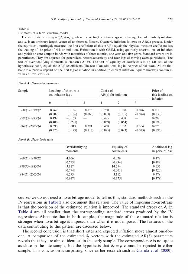
The results are displayed in Table 4. Panel A reports parameter estimates and Panel Breports specification tests. The first specification test is the Hansen (1982) J test ofoveridentifying restrictions. The second is a likelihood ratio (LR) test of the hypothesisdf ¼ r. This hypothesis means that short rates can be written as
rt ¼ d0 þ Eðptþ1jf tÞ þ ot. (70)
In other words, ex ante real short rates are uncorrelated with expected inflation. The LRtest has an asymptotic w2ðpÞ distribution under the null. The third is a Lagrange multiplier(LM) test of the hypothesis that the price of risk depends on the first two elements of f t
instead of just the first element. The LM test has an asymptotic w2ð1Þ distribution under thenull. The latter two test statistics are derived in Newey and West (1987b).There are three main conclusions to draw from these results. First, in both the early and
late samples there is a strong positive relation between the short rate and inflation. Of
ARTICLE IN PRESS
Table 4
Estimates of a term structure model
The short rate is rt ¼ d0 þ d0f f t þ d0xxt, where the vector f t contains lags zero through two of quarterly inflation
and xt is an arbitrary-length vector of unobserved factors. Quarterly inflation follows an AR(3) process. Under
the equivalent martingale measure, the first coefficient of this AR(3) equals the physical measure coefficient less
the loading of the price of risk on inflation. Estimation is with GMM, using quarterly observations of inflation
and yields on zero-coupon bonds with maturities of three months, one year, and five years. Standard errors are in
parentheses. They are adjusted for generalized heteroskedasticity and four lags of moving-average residuals. The
test of overidentifying moments is Hansen’s J test. The test of equality of coefficients is an LR test of the
hypothesis that df equals the AR(3) coefficients. The test of an additional lag in the price of risk is an LM test that
bond risk premia depend on the first lag of inflation in addition to current inflation. Square brackets contain p-
values of test statistics.
Panel A: Parameter estimates
Sample Loading of short rate Coef i of Price of
on inflation lag i AR(p) for inflation risk loading on
inflation
0 1 2 1 2 3
1960Q1–1979Q2 0.762 0.186 0.076 0.760 0.170 0.086 0.116
(0.202) (0.106) (0.065) (0.083) (0.135) (0.084) (0.038)
1979Q3–1983Q4 0.499 �0.159 — 0.485 0.408 — 0.092
(0.400) (0.291) (0.069) (0.054) (0.698)
1984Q1–2003Q4 0.590 0.319 0.291 0.458 0.102 0.364 0.026
(0.275) (0.149) (0.113) (0.075) (0.093) (0.073) (0.095)
Panel B: Hypothesis tests
Overidentifying Equality of Additional lag
moments coefficients in price of risk
1960Q1–1979Q2 4.666 0.079 0.479
[0.793] [0.994] [0.489]
1979Q3–1983Q4 3.117 14.254 0.652
[0.794] [0.001] [0.420]
1984Q1–2003Q4 6.273 3.112 0.778
[0.617] [0.375] [0.378]
G.R. Duffee / Journal of Financial Economics 79 (2006) 507–536 529
course, we do not need a no-arbitrage model to tell us this; standard methods such as theIV regressions in Table 2 also document this relation. The value of imposing no-arbitrageis that the precision of the estimated relation is improved. The standard errors on df inTable 4 are all smaller than the corresponding standard errors produced by the IVregressions. Also note that in both samples, the magnitude of the estimated relation isstronger when no-arbitrage is imposed than when it is not imposed. The features of thedata contributing to this pattern are discussed below.
The second conclusion is that short rates and expected inflation move almost one-for-one. A comparison of the estimated df vectors with the estimated AR(3) parametersreveals that they are almost identical in the early sample. The correspondence is not quiteas close in the late sample, but the hypothesis that df ¼ r cannot be rejected in eithersample. This conclusion is surprising, since earlier research such as Clarida et al. (2000),

ARTICLE IN PRESSG.R. Duffee / Journal of Financial Economics 79 (2006) 507–536530
Rudebusch (2002), and Goto and Torous (2003) document that short rates have beenmuch more sensitive to inflation rates in the post-deflationary sample than prior toVolcker’s tenure. These apparently conflicting results are resolved below.The third conclusion is that there is a modest inverse relation between inflation and bond
risk premia. All of the estimates of lff ð1Þ are positive, but only the early-sample estimate isstatistically different from zero. The connection between the sign of lff ð1Þ and the sign ofthe relation between inflation and risk premia is determined by (54). Higher inflationcorresponds to lower bond prices, which means that the log-price loadings on inflation,Bf ;t, are negative. Therefore, the product of lff ð1Þ and Bf ;t is negative, and from (54), higherinflation corresponds to lower expected excess returns.To get a sense of the magnitude of the reported coefficients, consider the standard
deviation of expected excess quarterly log returns to a five-year bond. The standarddeviation implied by the model can be computed with a combination of the formula forexpected excess returns (54) and the sample variance of the inflation state vector f t. For theearly sample, the implied standard deviation is 13.3 basis points, or 53 basis points on anannual basis. For the late sample, the implied standard deviation is only five basis pointson an annual basis.What features of the data drive the high estimated sensitivity of the short rate and the
low sensitivity of risk premia? To explore this question, take a closer look at the behaviorof bond yields during 1984Q1–2003Q4. Table 5 reports estimates of the relation betweenone-year and five-year bond yields and f t:
yt;t ¼ b0;t þ b0tf t þ et. (71)
The vector bt is calculated with three alternative techniques. The first technique differences(71) and estimates it with instrumental variables, paralleling the estimation of (64). Thesecond uses the IV estimate of (64) from Table 2, the AR(3) estimate of inflation fromTable 3, and the assumption that risk premia are invariant to f t. The vector bt is then givenby no-arbitrage (ignoring the requirement that the computed vector for the one-year yieldmust be consistent with the vector for the five-year yield). The third uses the parameter
Table 5
Loadings of longer-term bond yields on current and lagged inflation, 1984Q1–2003Q4
The yield on a t-maturity bond is expressed as yt;t ¼ b0 þ b1pt þ b2pt�1 þ b3pt�2 þ et;t, where pt is inflation
during quarter t. Estimated coefficients are produced using three methods. With ‘‘IV,’’ the equation is first-
differenced and estimated over 1984Q1–2003Q4 with instrumental variables. With ‘‘Short rate/constant premia,’’
the coefficients are calculated using (a) the estimate of the corresponding expression for the short rate, (b) the
estimate of the AR(3) dynamics of inflation, and (c) the assumption that risk premia are invariant to inflation.
With ‘‘Model,’’ the coefficients are calculated using a term structure model estimated over 1984Q1–2003Q4.
Maturity Method Loading of the yield on inflation lag i
0 1 2
One year IV 0.460 0.321 0.258
One year Short rate/constant premia 0.437 0.224 0.149
One year Model 0.574 0.303 0.233
Five years IV 0.379 0.216 0.257
Five years Short rate/constant premia 0.208 0.100 0.066
Five years Model 0.392 0.204 0.153

ARTICLE IN PRESSG.R. Duffee / Journal of Financial Economics 79 (2006) 507–536 531
estimates of the no-arbitrage model reported in Table 4 to compute bt. No standard errorsare reported in Table 5 because the only goal is to understand why the results of these threeprocedures differ from each other.
Intuitively, estimation of the no-arbitrage model with GMM produces loadings of yieldson f t that are as close as possible to the IV estimates of these factor loadings, subject to therequirement of no-arbitrage. A comparison of the first row of Table 5 with the secondreveals that the one-year yield is more sensitive to f t than is implied by the IV estimates ofshort-rate dynamics and constant risk premia. In fact, these IV estimates are larger thanthe corresponding IV estimates for the short rate reported in Table 2. To fit the IVestimates for the one-year yield, either the short rate needs to be more responsive toinflation or risk premia need to be high when inflation is high.
If we attempt to reconcile the IV estimates for the short rate and the one-year yieldsimply by adjusting the risk premia, no-arbitrage requires that the loadings for the five-year yield exceed the loadings for the one-year yield. (In other words, inflation must benonstationary under the equivalent martingale measure.) A comparison of the first andfourth rows of Table 5 reveals that this is counterfactual. Therefore, GMM estimationpicks short-rate loadings df that exceed the corresponding IV estimates, trading off fittingthe short rate with fitting the longer-maturity yields. The model-implied loadings for theone-year and five-year yields (the table’s third and sixth rows) are fairly close to the IV-estimated loadings, although the coefficients on contemporaneous inflation are too highand the coefficients on lagged inflation are too low. These loadings are produced with avalue of lff close to zero. If risk premia increased when inflation increased (negative lff ),the loadings on inflation would be larger. This would produce a better fit for the loadingson lagged inflation but a worse fit for the loadings on contemporaneous inflation.
As mentioned above, much research documents the high sensitivity of interest rates toinflation in the Volcker and Greenspan tenures. The results here do not support this result.The reason is that more recent data are used here. Table 6 reports estimation results for thepost-deflationary sample, with different ending points. The ending point of 1996Q4
Table 6
Estimates of a term structure model: Sample sensitivity
The short rate is rt ¼ d0 þ d0f f t þ d0xxt, where the vector f t contains lags zero through two of quarterly inflation
and xt is an arbitrary-length vector of unobserved factors. Quarterly inflation follows an AR(3) process. Under
the equivalent martingale measure, the first coefficient of this AR(3) equals the physical measure coefficient less
the loading of the price of risk on inflation. Estimation is with GMM, using quarterly observations of inflation
and yields on zero-coupon bonds with maturities of three months, one year, and five years. Standard errors are in
parentheses. They are adjusted for generalized heteroskedasticity and four lags of moving-average residuals.
Sample Loading of short rate Coef i of Price of
on inflation lag i AR(p) for inflation risk loading on
inflation
0 1 2 1 2 3
1984Q1–1996Q4 0.923 0.584 0.561 0.382 0.026 0.473 0.012
(0.235) (0.131) (0.130) (0.057) (0.103) (0.083) (0.079)
1984Q1–2001Q4 0.861 0.462 0.484 0.519 �0.018 0.477 0.053
(0.256) (0.125) (0.122) (0.074) (0.092) (0.074) (0.073)
1984Q1–2002Q4 0.157 0.090 0.139 0.544 �0.022 0.363 0.224
(0.308) (0.132) (0.121) (0.070) (0.084) (0.104) (0.356)

ARTICLE IN PRESS
1984 1986 1988 1990 1992 1994 1996 1998 2000 2002 2004
-0.14
-0.12
-0.1
-0.08
-0.06
-0.04
-0.02
0P
erce
nt
Predicted change in five−year yield
1984 1986 1988 1990 1992 1994 1996 1998 2000 2002 2004
-1.5
-1
-0.5
0
0.5
1
Date
Per
cent
Actual change in five−year yield
(A)
(B)
Fig. 1. A comparison of forecasted and actual quarterly changes in bond yields. At the end of quarter t� 1, the
change in the five-year bond yield from t� 1 to t is predicted using a term structure model. The model is estimated
using data through 2001Q4, while the one-quarter-ahead forecasts (plotted in Panel A) are constructed through
2003Q3. Panel B plots realized changes in yields. The plots are aligned so that the forecast made at t� 1 of the
quarter-t change corresponds to the quarter-t realization of this change.
G.R. Duffee / Journal of Financial Economics 79 (2006) 507–536532
matches that in Clarida et al. (2000). Consistent with their evidence, the no-arbitrageresults for this sample implies a very high sensitivity of the short rate to inflation. The sumof the coefficients on lags zero through two of the short rate exceeds two. Adding five yearsof data (an ending point of 2001Q4) does not substantially affect these results. However,including data for 2002 dramatically changes the results. With this sample, the estimatedloadings on inflation are economically small and statistically indistinguishable from zero.Fig. 1 helps explain these results. Panel A is constructed using the parameter estimates
from the no-arbitrage model estimated over 1984Q1–2001Q4. It plots one-quarter-aheadforecasts of changes in the five-year yield. The predicted changes are consistently negativebecause the model is fitting the general decline in interest rates during the sample. The lasttwo years are out-of-sample forecasts in the sense that the model is estimated without thesedata, although the forecast formed at quarter t� 1 uses inflation data through quartert� 1. Panel B shows the corresponding realization of the change in the five-year yield.(Note that the scales of the two figures do not correspond; realizations are much morevolatile than forecasts.)Inflation was very low during early 2002. Therefore the AR model of inflation forecasted
rising inflation in late 2002, and correspondingly rising bond yields. In Panel A, two of thelargest predicted changes in the five-year bond yield are the predictions formed in 2002Q1and 2002Q2 for changes in 2002Q2 and 2002Q3, respectively. However, bond yields fellsubstantially during 2002. In fact, the largest decline in the five-year yield during the entiresample occurred between 2002Q2 and 2002Q3. Thus, the forecasts are spectacularly wrong

ARTICLE IN PRESSG.R. Duffee / Journal of Financial Economics 79 (2006) 507–536 533
in 2002. The forecast accuracy improves in 2003, which is why estimation over the entiresample finds a statistically strong relation between inflation and bond yields.
3.6. Does the evidence support the model?
In both the pre-Volcker and post-disinflation samples, the formal tests of theoveridentifying restrictions do not come close to rejecting the model. Yet in a broadersense, these results reinforce existing evidence that a single regime is an unsatisfactorydescription of the joint dynamics of inflation and the term structure. Estimation of themodel over the entire sample 1960Q1 through 2003Q4 produces inflation factor loadings df
that are negative, much like the IV estimates reported in Table 2 for the entire sample. (Thefull-sample results of the no-arbitrage model are not reported in any table.) As previouslydiscussed in the context of these IV estimates, the problem with the full sample is thatinflation dynamics have varied substantially over time.
A more general no-arbitrage model needs to incorporate time-variation in inflationdynamics. One approach is to allow the parameters to switch at particular break points,but nevertheless price bonds as if investors believe parameters are constant over time. Thisis effectively the procedure followed here. An alternative approach is to allow for regimechanges in inflation dynamics, where investors recognize the possibility of regime changes.Unfortunately, tractable bond pricing in a regime-switching framework requires a numberof restrictions on the nature of the regime switching; not all of the components of thedynamics are allowed to switch regimes. The requirement of tractability leads to a varietyof nonnested regime-switching models. For example, the model of Ang and Bekaert (2003)cannot accommodate changing factor dynamics, while the model of Dai et al. (2003) allowsfor changing factor dynamics only by imposing tight restrictions on the dynamics of theprice of interest rate risk. Ang and Bekaert (2003) discuss the modeling advantages anddisadvantages of regime-switching factor dynamics. The results here suggest that arelatively simple regime-switching framework can accurately fit these data. There is noneed to allow for regime changes in the compensation investors require to bear inflationrisk. In addition, the short rate’s sensitivity to one-step-ahead forecasted inflation can beconstant across regimes. The only component that must shift regimes is the AR processfollowed by inflation. Whether these simple dynamics are consistent with a tractable bondpricing framework is an open question.
4. Concluding comments
This paper makes two contributions to the term structure literature. First, amethodological framework is constructed to investigate the relation between the termstructure and other observable variables. The framework imposes no-arbitrage withoutrequiring the estimation of the complete description of the term structure’s dynamics.Therefore, it can be used to describe the dynamics of expected returns to bonds conditionalon the observable variables. The framework is simple to implement with GMM because itis essentially a set of regressions that are estimated with either OLS or instrumentalvariables. Cross-equation restrictions implied by no-arbitrage allow us to infer theparameters of the model from these regressions.
Second, the framework is applied to the relation between inflation and the termstructure. The results suggest a simple description of this relation: short-term interest rates
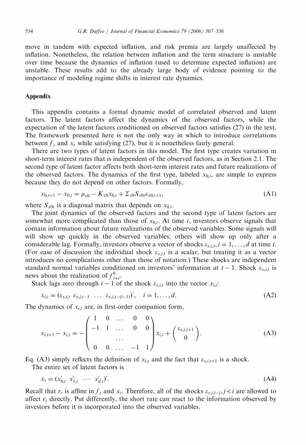
ARTICLE IN PRESSG.R. Duffee / Journal of Financial Economics 79 (2006) 507–536534
move in tandem with expected inflation, and risk premia are largely unaffected byinflation. Nonetheless, the relation between inflation and the term structure is unstableover time because the dynamics of inflation (used to determine expected inflation) areunstable. These results add to the already large body of evidence pointing to theimportance of modeling regime shifts in interest rate dynamics.
Appendix
This appendix contains a formal dynamic model of correlated observed and latentfactors. The latent factors affect the dynamics of the observed factors, while theexpectation of the latent factors conditioned on observed factors satisfies (27) in the text.The framework presented here is not the only way in which to introduce correlationsbetween f t and xt while satisfying (27), but it is nonetheless fairly general.There are two types of latent factors in this model. The first type creates variation in
short-term interest rates that is independent of the observed factors, as in Section 2.1. Thesecond type of latent factor affects both short-term interest rates and future realizations ofthe observed factors. The dynamics of the first type, labeled x0;t, are simple to expressbecause they do not depend on other factors. Formally,
x0;tþ1 � x0;t ¼ mx0 � Kx0x0;t þ Sx0Sx0t�x0;tþ1, (A1)
where Sx0t is a diagonal matrix that depends on x0;t.The joint dynamics of the observed factors and the second type of latent factors are
somewhat more complicated than those of x0;t. At time t, investors observe signals thatcontain information about future realizations of the observed variables. Some signals willwill show up quickly in the observed variables; others will show up only after aconsiderable lag. Formally, investors observe a vector of shocks �x;i;t; i ¼ 1; . . . ; d at time t.(For ease of discussion the individual shock �x;i;t is a scalar, but treating it as a vectorintroduces no complications other than those of notation.) These shocks are independentstandard normal variables conditioned on investors’ information at t� 1. Shock �x;i;t isnews about the realization of f 0
tþi.Stack lags zero through i � 1 of the shock �x;i;t into the vector xi;t:
xi;t ¼ ð�x;i;t �x;i;t�1 . . . �x;i;t�ði�1ÞÞ0; i ¼ 1; . . . ; d. (A2)
The dynamics of xi;t are, in first-order companion form,
xi;tþ1 � xi;t ¼ �
1 0 . . . 0 0
�1 1 . . . 0 0
. . .
0 0 . . . �1 1
0BBB@
1CCCAxi;t þ
�x;i;tþ1
0
� �. (A3)
Eq. (A3) simply reflects the definition of xi;t and the fact that �x;i;tþ1 is a shock.The entire set of latent factors is
xt ¼ ðx00;t x01;t � � � x0d;tÞ
0. (A4)
Recall that rt is affine in f t and xt. Therefore, all of the shocks �x;i;t�j ; joi are allowed toaffect rt directly. Put differently, the short rate can react to the information observed byinvestors before it is incorporated into the observed variables.

ARTICLE IN PRESSG.R. Duffee / Journal of Financial Economics 79 (2006) 507–536 535
At time tþ i, the observed variables f 0tþi react to �x;i;t. The key restriction built into their
relation is that after tþ 1, the shock has no direct effect on the observed variables. It onlyaffects these observed variables indirectly, through the persistence of the observedvariables themselves. The observed-factor dynamics satisfy (28) in the text, where thematrix Kfx is
Kfx ¼Kfx0 Kfx1 . . . Kfxd
0 0 . . . 0
� �, (A5)
Kfx0 ¼ 0; Kfxi ¼ ð0 kiÞ. (A6)
The submatrices of zeros in the second row of Kfx are a consequence of the first-ordercompanion form of (28). The matrix Kfx0 is zero because the latent factors x0;t areindependent of the observed factors. The submatrix of zeros in Kfxi is n0 � ði � 1Þ and ki isa vector of length n0. This structure implies that the shock �x;i;t does not affect the observedfactors until tþ i, at which point its effect is determined by the elements of ki.
It is easy to verify that these dynamics satisfy (27). The key intuition is that the vector xi;t
contains shocks that show up in the observed factors at tþ 1; . . . ; tþ i. Thus, it isindependent of f t�j ; jX0.
References
Ang, A., Bekaert, G., 2003. The term structure of real rates and expected inflation. Working Paper, Columbia
Business School.
Ang, A., Piazzesi, M., 2003. A no-arbitrage vector autoregression of term structure dynamics with
macroeconomic and latent variables. Journal of Monetary Economics 50, 745–787.
Ang, A., Piazzesi, M., Wei, M., 2005. What does the yield curve tell us about GDP growth? Journal of Monetary
Economics, forthcoming.
Campbell, J., Lo, A., MacKinlay, A., 1997. The Econometrics of Financial Markets. Princeton University Press,
Princeton.
Campbell, J., Shiller, R., 1991. Yield spreads and interest rate movements: a bird’s eye view. Review of Economic
Studies 58, 495–514.
Clarida, R., Galı, J., Gertler, M., 2000. Monetary policy rules and macroeconomic stability: evidence and some
theory. Quarterly Journal of Economics 115, 147–180.
Cox, J., Ingersoll, J., Ross, S., 1985. A theory of the term structure of interest rates. Econometrica 53, 385–407.
Dai, Q., Singleton, K., Yang, W., 2003. Regime shifts in a dynamic term structure model of U.S. Treasury bond
yields. Working Paper, Stern School of Business.
Dewachter, H., Lyrio, M., 2002. Macro factors and the term structure of interest rates. Working Paper, Catholic
University of Leuven.
Dewachter, H., Lyrio, M., Maes, K., 2002. Estimation of a joint model for the term structure of interest rates and
the macroeconomy. Working Paper, Catholic University of Leuven.
Diebold, F., Rudebusch, G., Aruoba, S., 2003. The macroeconomy and the yield curve: a nonstructural analysis.
Working Paper, The Wharton School.
Duffee, G., 2002. Term premia and interest rate forecasts in affine models. Journal of Finance 57, 405–443.
Duffie, D., Kan, R., 1996. A yield-factor model of interest rates. Mathematical Finance 6, 379–406.
English, W., Nelson, W., Sack, B., 2003. Interpreting the significance of the lagged interest rate in estimated
monetary policy rules. Contributions to Macroeconomics 3, Article 5.
Fama, E., 1975. Short-term interest rates as predictors of inflation. American Economic Review 65, 269–282.
Goto, S., Torous, W., 2003. The conquest of U.S. inflation: its implications for the Fisher hypothesis and the term
structure of nominal interest rates. Working Paper, University of South Carolina.
Gray, S., 1996. Modeling the conditional distribution of interest rates as a regime-switching process. Journal of
Financial Economics 42, 27–62.

ARTICLE IN PRESSG.R. Duffee / Journal of Financial Economics 79 (2006) 507–536536
Hansen, L., 1982. Large sample properties of generalized method of moment estimators. Econometrica 50,
1029–1053.
Hansen, L., Singleton, K., 1982. Generalized instrumental variables estimators of nonlinear rational expectations
models. Econometrica 50, 1269–1286.
Hordahl, P., Tristani, O., Vestin, D., 2002. A joint econometric model of macroeconomic and term structure
dynamics. Working Paper, European Central Bank.
Kimmel, R., Cheridito, P., Filipovic, D., 2004. Market price of risk specification for affine models: theory and
evidence. Working Paper, Princeton University.
Newey, W., West, K., 1987a. A simple, positive semi-definite, heteroskedasticity and autocorrelation consistent
covariance matrix. Econometrica 55, 703–708.
Newey, W., West, K., 1987b. Hypothesis testing with efficient method of moments estimation. International
Economic Review 28, 777–787.
Piazzesi, M., 2005. Bond yields and the Federal Reserve. Journal of Political Economy 113, 311–344.
Rudebusch, G., 2002. Term structure evidence on interest rate smoothing and monetary policy inertia. Journal of
Monetary Economics 49, 1161–1187.
Rudebusch, G., Wu, T., 2003. A macro-finance model of the term structure, monetary policy, and the economy.
Working Paper, Federal Reserve Bank of San Francisco.
Sack, B., Wieland, V., 2000. Interest-rate smoothing and optimal monetary policy: a review of recent empirical
evidence. Journal of Economics and Business 52, 205–228.
Taylor, J., 1993. Discretion versus policy rules in practice. Carnegie-Rochester Conference Series on Public Policy
39, 195–214.
Vasicek, O., 1977. An equilibrium characterization of the term structure. Journal of Financial Economics 5,
177–188.