Embed Size (px)
Citation preview
CHAPTER 5
Tensors and the Equations of Fluid Motion
We have seen that there are a whole range of things that we can represent onthe computer. We have solved some simple problems such as Laplace’s equationon a unit square at the origin in the first quadrant. From the description of theproblem, you can see that it was really a very specific problem. Our objective wasto dive into the process of representing and solving partial differential equations onthe computer and we have achieved that objective. The problem was simple enoughthat we could analyse the resulting discrete equations. Similarly, we have studiedthe first order one-dimensional linear wave equation. We have also seen the heatequation and the quasi linear version of the wave equation. We have some basicunderstanding of the issues involved in representing and solving these problems onthe computer. We are now in a position to solve a larger class of problems. We willexpand on the simple problems we studied in the preceding chapters as a meansto motivate this chapter. We will then do the essentials of tensor calculus requiredto derive the equations of fluid motion. The equations of motion will be derivedin vector form so as to be independent of the particular coordinate system. Takenalong with the tensor calculus you should be able to specialise these equations toany particular coordinate system.
5.1. Laplace Equation Revisited
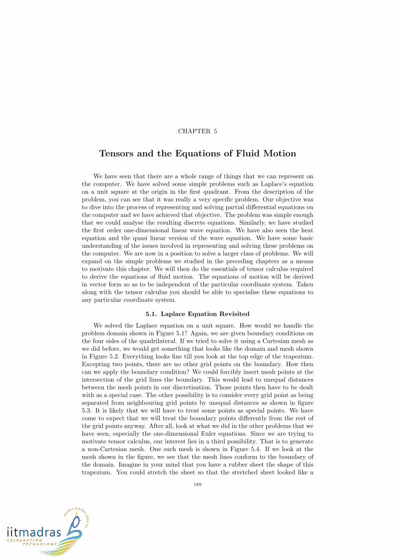
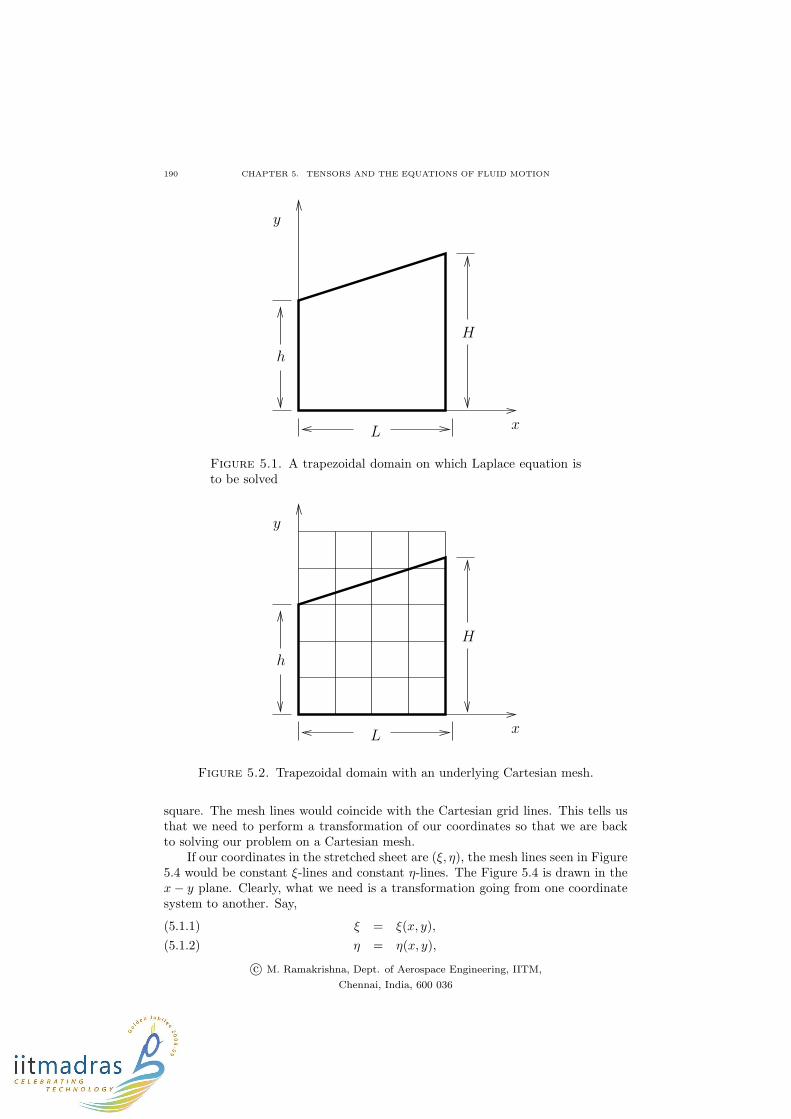
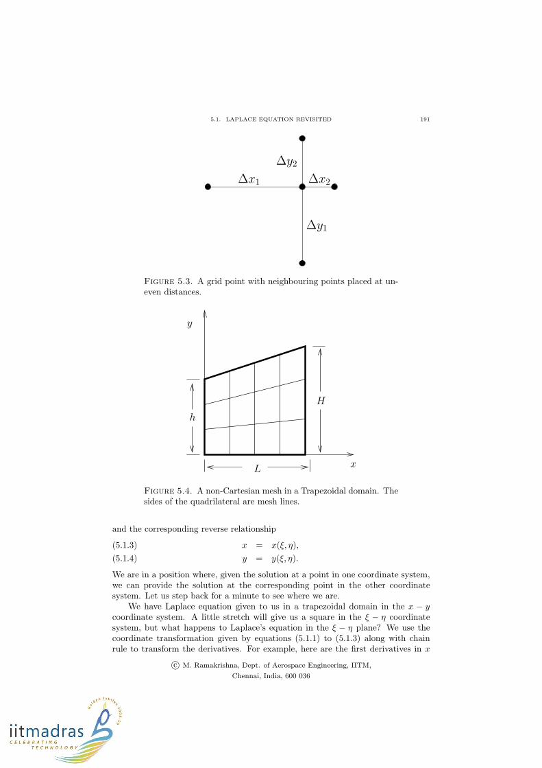
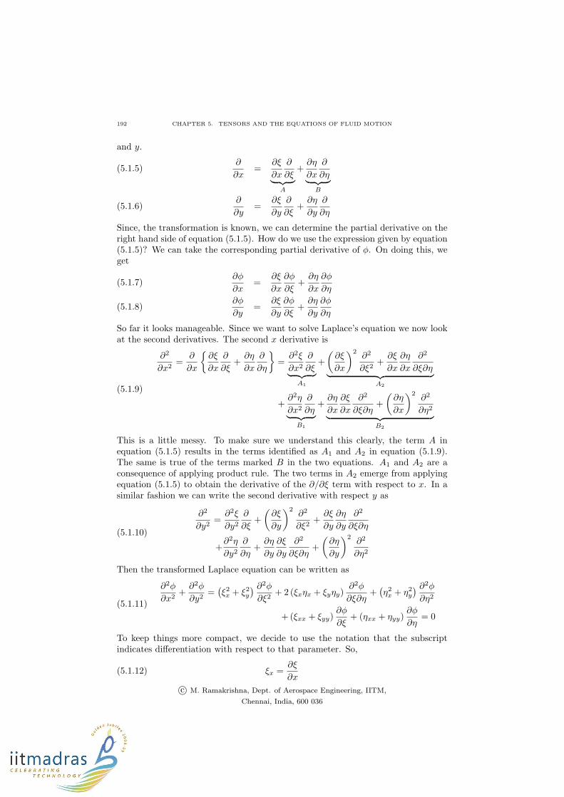
We solved the Laplace equation on a unit square. How would we handle theproblem domain shown in Figure 5.1? Again, we are given boundary conditions onthe four sides of the quadrilateral. If we tried to solve it using a Cartesian mesh aswe did before, we would get something that looks like the domain and mesh shownin Figure 5.2. Everything looks fine till you look at the top edge of the trapezium.Excepting two points, there are no other grid points on the boundary. How thencan we apply the boundary condition? We could forcibly insert mesh points at theintersection of the grid lines the boundary. This would lead to unequal distancesbetween the mesh points in our discretisation. Those points then have to be dealtwith as a special case. The other possibility is to consider every grid point as beingseparated from neighbouring grid points by unequal distances as shown in figure5.3. It is likely that we will have to treat some points as special points. We havecome to expect that we will treat the boundary points differently from the rest ofthe grid points anyway. After all, look at what we did in the other problems that wehave seen, especially the one-dimensional Euler equations. Since we are trying tomotivate tensor calculus, our interest lies in a third possibility. That is to generatea non-Cartesian mesh. One such mesh is shown in Figure 5.4. If we look at themesh shown in the figure, we see that the mesh lines conform to the boundary ofthe domain. Imagine in your mind that you have a rubber sheet the shape of thistrapezium. You could stretch the sheet so that the stretched sheet looked like a
189
190 CHAPTER 5. TENSORS AND THE EQUATIONS OF FLUID MOTION
x
y
L
h
H
Figure 5.1. A trapezoidal domain on which Laplace equation isto be solved
x
y
L
h
H
Figure 5.2. Trapezoidal domain with an underlying Cartesian mesh.
square. The mesh lines would coincide with the Cartesian grid lines. This tells usthat we need to perform a transformation of our coordinates so that we are backto solving our problem on a Cartesian mesh.
If our coordinates in the stretched sheet are (ξ, η), the mesh lines seen in Figure5.4 would be constant ξ-lines and constant η-lines. The Figure 5.4 is drawn in thex− y plane. Clearly, what we need is a transformation going from one coordinatesystem to another. Say,
ξ = ξ(x, y),(5.1.1)
η = η(x, y),(5.1.2)
c© M. Ramakrishna, Dept. of Aerospace Engineering, IITM,
Chennai, India, 600 036
5.1. LAPLACE EQUATION REVISITED 191
∆y1
∆x2∆x1
∆y2
Figure 5.3. A grid point with neighbouring points placed at un-even distances.
x
y
L
h
H
Figure 5.4. A non-Cartesian mesh in a Trapezoidal domain. Thesides of the quadrilateral are mesh lines.
and the corresponding reverse relationship
x = x(ξ, η),(5.1.3)
y = y(ξ, η).(5.1.4)
We are in a position where, given the solution at a point in one coordinate system,we can provide the solution at the corresponding point in the other coordinatesystem. Let us step back for a minute to see where we are.
We have Laplace equation given to us in a trapezoidal domain in the x − ycoordinate system. A little stretch will give us a square in the ξ − η coordinatesystem, but what happens to Laplace’s equation in the ξ − η plane? We use thecoordinate transformation given by equations (5.1.1) to (5.1.3) along with chainrule to transform the derivatives. For example, here are the first derivatives in x
c© M. Ramakrishna, Dept. of Aerospace Engineering, IITM,
Chennai, India, 600 036
192 CHAPTER 5. TENSORS AND THE EQUATIONS OF FLUID MOTION
and y.
∂
∂x=
∂ξ
∂x
∂
∂ξ︸ ︷︷ ︸
A
+∂η
∂x
∂
∂η︸ ︷︷ ︸
B
(5.1.5)
∂
∂y=
∂ξ
∂y
∂
∂ξ+∂η
∂y
∂
∂η(5.1.6)
Since, the transformation is known, we can determine the partial derivative on theright hand side of equation (5.1.5). How do we use the expression given by equation(5.1.5)? We can take the corresponding partial derivative of φ. On doing this, weget
∂φ
∂x=
∂ξ
∂x
∂φ
∂ξ+∂η
∂x
∂φ
∂η(5.1.7)
∂φ
∂y=
∂ξ
∂y
∂φ
∂ξ+∂η
∂y
∂φ
∂η(5.1.8)
So far it looks manageable. Since we want to solve Laplace’s equation we now lookat the second derivatives. The second x derivative is
∂2
∂x2=
∂
∂x
{∂ξ
∂x
∂
∂ξ+∂η
∂x
∂
∂η
}
=∂2ξ
∂x2
∂
∂ξ︸ ︷︷ ︸
A1
+
(∂ξ
∂x
)2∂2
∂ξ2+∂ξ
∂x
∂η
∂x
∂2
∂ξ∂η︸ ︷︷ ︸
A2
+∂2η
∂x2
∂
∂η︸ ︷︷ ︸
B1
+∂η
∂x
∂ξ
∂x
∂2
∂ξ∂η+
(∂η
∂x
)2∂2
∂η2
︸ ︷︷ ︸
B2
(5.1.9)
This is a little messy. To make sure we understand this clearly, the term A inequation (5.1.5) results in the terms identified as A1 and A2 in equation (5.1.9).The same is true of the terms marked B in the two equations. A1 and A2 are aconsequence of applying product rule. The two terms in A2 emerge from applyingequation (5.1.5) to obtain the derivative of the ∂/∂ξ term with respect to x. In asimilar fashion we can write the second derivative with respect y as
∂2
∂y2=∂2ξ
∂y2
∂
∂ξ+
(∂ξ
∂y
)2∂2
∂ξ2+∂ξ
∂y
∂η
∂y
∂2
∂ξ∂η
+∂2η
∂y2
∂
∂η+∂η
∂y
∂ξ
∂y
∂2
∂ξ∂η+
(∂η
∂y
)2∂2
∂η2
(5.1.10)
Then the transformed Laplace equation can be written as
∂2φ
∂x2+∂2φ
∂y2=
(ξ2x + ξ2y
) ∂2φ
∂ξ2+ 2 (ξxηx + ξyηy)
∂2φ
∂ξ∂η+
(η2
x + η2y
) ∂2φ
∂η2
+(ξxx + ξyy)∂φ
∂ξ+ (ηxx + ηyy)
∂φ
∂η= 0
(5.1.11)
To keep things more compact, we decide to use the notation that the subscriptindicates differentiation with respect to that parameter. So,
(5.1.12) ξx =∂ξ
∂x
c© M. Ramakrishna, Dept. of Aerospace Engineering, IITM,
Chennai, India, 600 036
5.1. LAPLACE EQUATION REVISITED 193
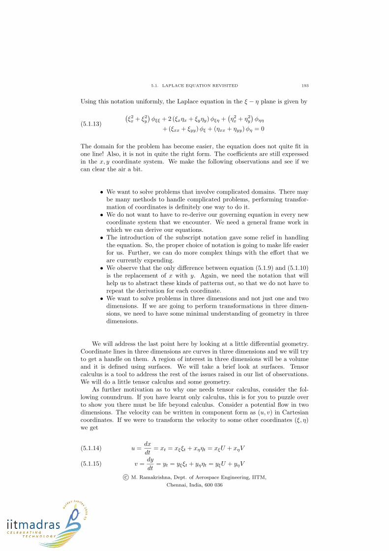
Using this notation uniformly, the Laplace equation in the ξ − η plane is given by
(ξ2x + ξ2y
)φξξ + 2 (ξxηx + ξyηy)φξη +
(η2
x + η2y
)φηη
+(ξxx + ξyy)φξ + (ηxx + ηyy)φη = 0(5.1.13)
The domain for the problem has become easier, the equation does not quite fit inone line! Also, it is not in quite the right form. The coefficients are still expressedin the x, y coordinate system. We make the following observations and see if wecan clear the air a bit.
• We want to solve problems that involve complicated domains. There maybe many methods to handle complicated problems, performing transfor-mation of coordinates is definitely one way to do it.
• We do not want to have to re-derive our governing equation in every newcoordinate system that we encounter. We need a general frame work inwhich we can derive our equations.
• The introduction of the subscript notation gave some relief in handlingthe equation. So, the proper choice of notation is going to make life easierfor us. Further, we can do more complex things with the effort that weare currently expending.
• We observe that the only difference between equation (5.1.9) and (5.1.10)is the replacement of x with y. Again, we need the notation that willhelp us to abstract these kinds of patterns out, so that we do not have torepeat the derivation for each coordinate.
• We want to solve problems in three dimensions and not just one and twodimensions. If we are going to perform transformations in three dimen-sions, we need to have some minimal understanding of geometry in threedimensions.
We will address the last point here by looking at a little differential geometry.Coordinate lines in three dimensions are curves in three dimensions and we will tryto get a handle on them. A region of interest in three dimensions will be a volumeand it is defined using surfaces. We will take a brief look at surfaces. Tensorcalculus is a tool to address the rest of the issues raised in our list of observations.We will do a little tensor calculus and some geometry.
As further motivation as to why one needs tensor calculus, consider the fol-lowing conundrum. If you have learnt only calculus, this is for you to puzzle overto show you there must be life beyond calculus. Consider a potential flow in twodimensions. The velocity can be written in component form as (u, v) in Cartesiancoordinates. If we were to transform the velocity to some other coordinates (ξ, η)we get
u =dx
dt= xt = xξξt + xηηt = xξU + xηV(5.1.14)
v =dy
dt= yt = yξξt + yηηt = yξU + yηV(5.1.15)
c© M. Ramakrishna, Dept. of Aerospace Engineering, IITM,
Chennai, India, 600 036
194 CHAPTER 5. TENSORS AND THE EQUATIONS OF FLUID MOTION
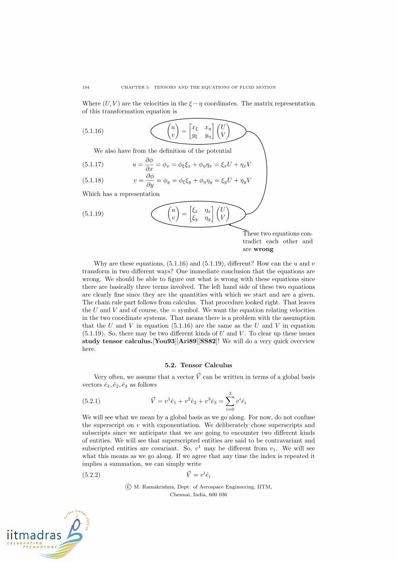
Where (U, V ) are the velocities in the ξ−η coordinates. The matrix representationof this transformation equation is
(5.1.16)
(uv
)
=
[xξ xη
yξ yη
](UV
)
We also have from the definition of the potential
u =∂φ
∂x= φx = φξξx + φηηx = ξxU + ηxV(5.1.17)
v =∂φ
∂y= φy = φξξy + φηηy = ξyU + ηyV(5.1.18)
Which has a representation
(5.1.19)
(uv
)
=
[ξx ηx
ξy ηy
] (UV
)
These two equations con-tradict each other andare wrong
Why are these equations, (5.1.16) and (5.1.19), different? How can the u and vtransform in two different ways? One immediate conclusion that the equations arewrong. We should be able to figure out what is wrong with these equations sincethere are basically three terms involved. The left hand side of these two equationsare clearly fine since they are the quantities with which we start and are a given.The chain rule part follows from calculus. That procedure looked right. That leavesthe U and V and of course, the = symbol. We want the equation relating velocitiesin the two coordinate systems. That means there is a problem with the assumptionthat the U and V in equation (5.1.16) are the same as the U and V in equation(5.1.19). So, there may be two different kinds of U and V . To clear up these issuesstudy tensor calculus.[You93][Ari89][SS82]! We will do a very quick overviewhere.
5.2. Tensor Calculus
Very often, we assume that a vector ~V can be written in terms of a global basisvectors e1, e2, e3 as follows
(5.2.1) ~V = v1e1 + v2e2 + v3e3 =3∑
i=0
viei
We will see what we mean by a global basis as we go along. For now, do not confusethe superscript on v with exponentiation. We deliberately chose superscripts andsubscripts since we anticipate that we are going to encounter two different kindsof entities. We will see that superscripted entities are said to be contravariant andsubscripted entities are covariant. So, v1 may be different from v1. We will seewhat this means as we go along. If we agree that any time the index is repeated itimplies a summation, we can simply write
(5.2.2) ~V = viei
c© M. Ramakrishna, Dept. of Aerospace Engineering, IITM,
Chennai, India, 600 036

5.2. TENSOR CALCULUS 195
Now, THAT is compact. It is called Einstein’s summation convention. It onlygets better. By itself, the equation does not even restrict us to three dimensions.It is our assumption that we use three dimensions. In this book, we will restrictourselves to two / three dimensions. You should note that
(5.2.3) ~V = viei = vkek
Since there is a summation over the index, the index itself does not survive thesummation operation. The choice of the index is left to us. It is called a dummy
index.
1
2
3
P
Q
~x(P )
~x(Q)
Figure 5.5. A Cartesian coordinate system used to locate thepoint P and Q. ~x(P ) gives the position vector of P in the Carte-sian coordinate system. PQ forms a differential element.
We now define the notation with respect to coordinate systems. Consider Fig-ure 5.5. It indicates a differential line element with two points P and Q at each endof the element. We define ~x(.) as a coordinate function which returns the coordi-nates of a point in the Cartesian coordinate system. If we had another coordinatesystem overlayed on the same region, the point P will have the corresponding co-
ordinates ~ξ(P ) in that coordinate system. The coordinate function is simple toimagine if we look at it component-wise.
(5.2.4) ~x(P ) = x1(P )e1 + x2(P )e2 + x3(P )e3
Since we are dealing with Cartesian coordinates, xi and xi are the same. we have
already seen that if ~P is the position vector for P then
(5.2.5) xi(P ) = ~P · ei
c© M. Ramakrishna, Dept. of Aerospace Engineering, IITM,
Chennai, India, 600 036

196 CHAPTER 5. TENSORS AND THE EQUATIONS OF FLUID MOTION
Consider the problem of coordinate transformations in two dimensions. Let usrestrict ourselves for the sake of this discussion to rotations. We take our standardx − y coordinate and rotate through an angle θ to get the ξ − η coordinates. Thebasis vectors in x− y are ~e1 and ~e2. The basis vectors in the ξ − η coordinates are~ǫ1 and ~ǫ2. You can check that the basis vectors are related as follows:
(5.2.6)
(~ǫ1~ǫ2
)
=
[cos θ sin θ− sin θ cos θ
](~e1~e2
)
We see that by using indices we can simply represent this as
(5.2.7) ~ǫi = Aji~ej
Now, a vector ~s can be represented in the x−y and the ξ−η coordinate systemsas
(5.2.8) ~s = si~ei = ψi~ǫi
Substituting for ~ǫi from equation (5.2.7) we get
(5.2.9) ~s = si~ei = sj~ej = ψi~ǫi = ψiAji~ej
where i and j are dummy indices. Even though they are dummy indices, by theproper choice of these dummy indices here we can conclude that
(5.2.10) sj = ψiAji = Aj
iψi
Compare equations (5.2.7) and (5.2.10). The unit vectors transform one way,the components transform the opposite [ or contra ] way. We see that they too showthe same behaviour we saw with the velocity potential. Vectors that transform likeeach other are covariant with each other. Vectors that transform the opposite wayare contravariant to each other. This is too broad a scenario for us. We will stickwith something simpler. Covariant entities will be subscripted. Contravariant
entities will be superscripted.An example where this will be obvious to you is the case of the rotation of
the Cartesian coordinate system. Again, we restrict ourselves to two dimensions.If you rotate the standard Cartesian coordinate system counter-clockwise, you seethat the coordinate lines and the unit vectors ( as expected ) rotate in the samedirection. They are covariant. The actual coordinate values do not change in thesame fashion. In fact, the new values corresponding to a position vector look asthough the coordinate system was fixed and that the position vector was rotated ina clockwise sense ( contra or opposite to the original coordinate rotation ). Thesetwo rotations are in fact of equal magnitude and opposite in sense. They are, indeed,inverses of each other. We will investigate covariant and contravariant quantitiesmore as we go along. Right now, we have assumed that we have a position vector.Let us take a closer look at this.
We have made one assumption so far that the basis vector is global. We usedthe term global basis in the beginning of this section. What do we mean by aglobal basis? We want the basis to be the same, that is constant, at every point.Such a set of basis vectors is also said to be homogeneous. For example, the basisvectors in the standard Cartesian coordinate system do not depend on the (x, y)coordinates of a point. Consider the trapezium in Figure (5.7) We see that thetangent to the η = constant coordinate lines change with η. In general, the basisvectors change from point to point. We do not have a global basis. Also, consider
c© M. Ramakrishna, Dept. of Aerospace Engineering, IITM,
Chennai, India, 600 036
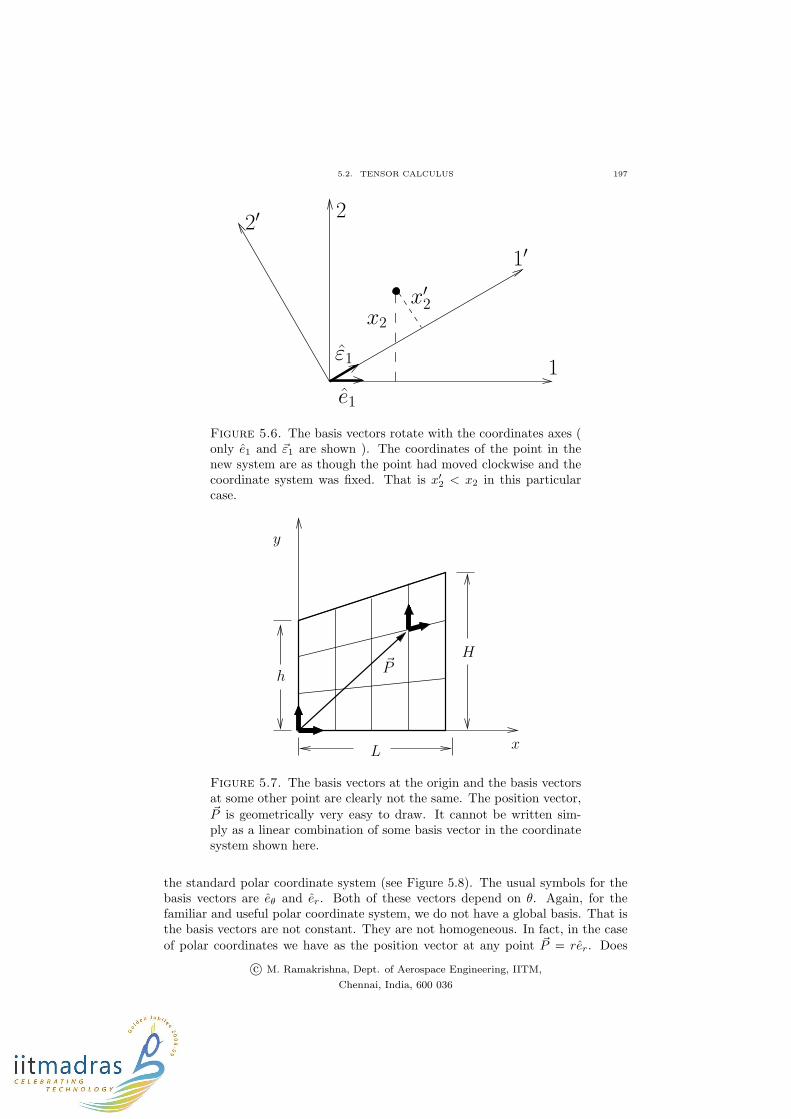
5.2. TENSOR CALCULUS 197
e1
1
1′
22′
ε1
x′2
x2
Figure 5.6. The basis vectors rotate with the coordinates axes (only e1 and ~ε1 are shown ). The coordinates of the point in thenew system are as though the point had moved clockwise and thecoordinate system was fixed. That is x′2 < x2 in this particularcase.
x
y
L
h
H~P
Figure 5.7. The basis vectors at the origin and the basis vectorsat some other point are clearly not the same. The position vector,~P is geometrically very easy to draw. It cannot be written sim-ply as a linear combination of some basis vector in the coordinatesystem shown here.
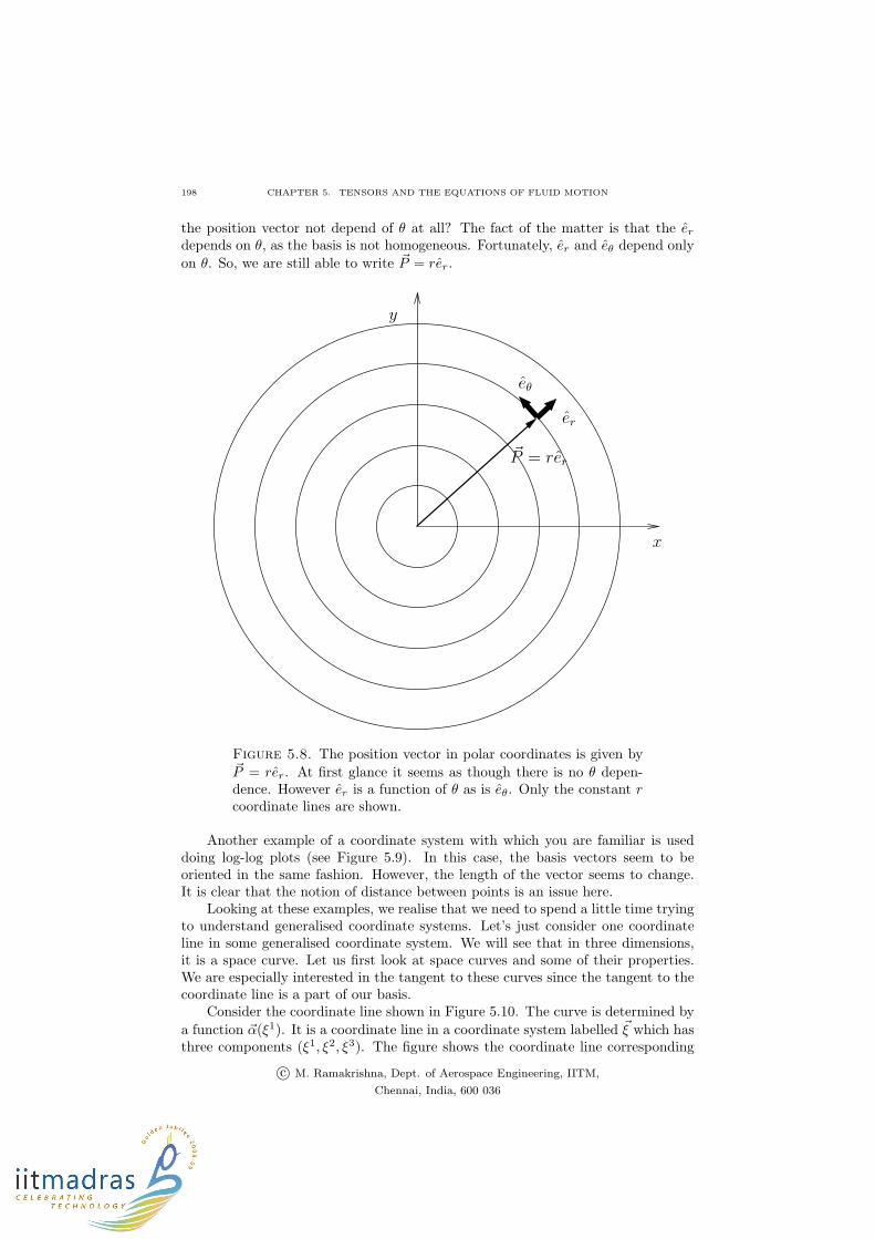
the standard polar coordinate system (see Figure 5.8). The usual symbols for thebasis vectors are eθ and er. Both of these vectors depend on θ. Again, for thefamiliar and useful polar coordinate system, we do not have a global basis. That isthe basis vectors are not constant. They are not homogeneous. In fact, in the case
of polar coordinates we have as the position vector at any point ~P = rer. Does
c© M. Ramakrishna, Dept. of Aerospace Engineering, IITM,
Chennai, India, 600 036
198 CHAPTER 5. TENSORS AND THE EQUATIONS OF FLUID MOTION
the position vector not depend of θ at all? The fact of the matter is that the er
depends on θ, as the basis is not homogeneous. Fortunately, er and eθ depend only
on θ. So, we are still able to write ~P = rer.
x
y
er
eθ
~P = rer
Figure 5.8. The position vector in polar coordinates is given by~P = rer. At first glance it seems as though there is no θ depen-dence. However er is a function of θ as is eθ. Only the constant rcoordinate lines are shown.
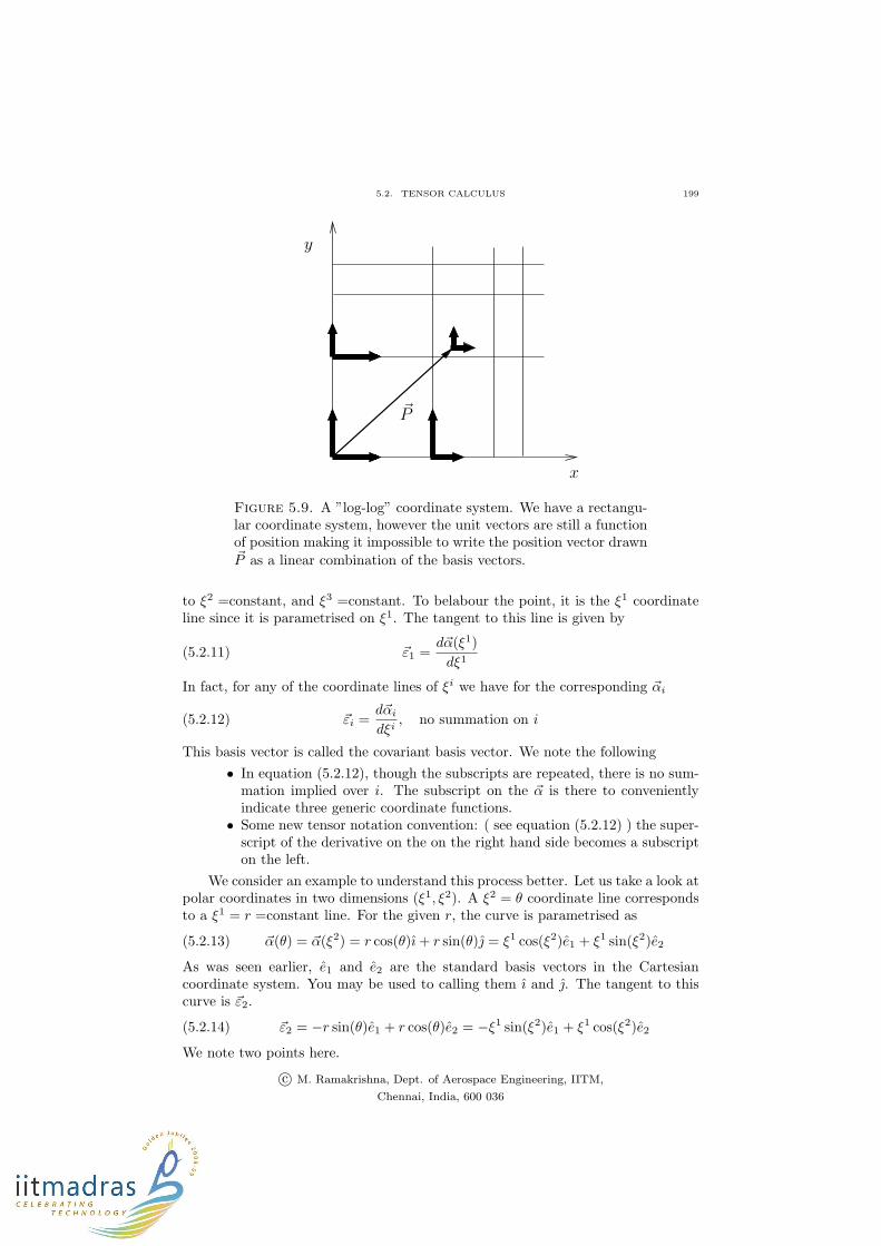
Another example of a coordinate system with which you are familiar is useddoing log-log plots (see Figure 5.9). In this case, the basis vectors seem to beoriented in the same fashion. However, the length of the vector seems to change.It is clear that the notion of distance between points is an issue here.
Looking at these examples, we realise that we need to spend a little time tryingto understand generalised coordinate systems. Let’s just consider one coordinateline in some generalised coordinate system. We will see that in three dimensions,it is a space curve. Let us first look at space curves and some of their properties.We are especially interested in the tangent to these curves since the tangent to thecoordinate line is a part of our basis.
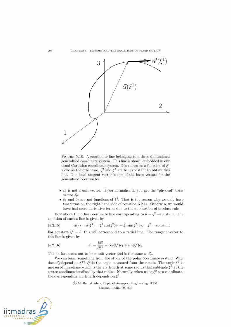
Consider the coordinate line shown in Figure 5.10. The curve is determined by
a function ~α(ξ1). It is a coordinate line in a coordinate system labelled ~ξ which hasthree components (ξ1, ξ2, ξ3). The figure shows the coordinate line corresponding
c© M. Ramakrishna, Dept. of Aerospace Engineering, IITM,
Chennai, India, 600 036
5.2. TENSOR CALCULUS 199
x
y
~P
Figure 5.9. A ”log-log” coordinate system. We have a rectangu-lar coordinate system, however the unit vectors are still a functionof position making it impossible to write the position vector drawn~P as a linear combination of the basis vectors.
to ξ2 =constant, and ξ3 =constant. To belabour the point, it is the ξ1 coordinateline since it is parametrised on ξ1. The tangent to this line is given by
(5.2.11) ~ε1 =d~α(ξ1)
dξ1
In fact, for any of the coordinate lines of ξi we have for the corresponding ~αi
(5.2.12) ~εi =d~αi
dξi, no summation on i
This basis vector is called the covariant basis vector. We note the following
• In equation (5.2.12), though the subscripts are repeated, there is no sum-mation implied over i. The subscript on the ~α is there to convenientlyindicate three generic coordinate functions.
• Some new tensor notation convention: ( see equation (5.2.12) ) the super-script of the derivative on the on the right hand side becomes a subscripton the left.
We consider an example to understand this process better. Let us take a look atpolar coordinates in two dimensions (ξ1, ξ2). A ξ2 = θ coordinate line correspondsto a ξ1 = r =constant line. For the given r, the curve is parametrised as
(5.2.13) ~α(θ) = ~α(ξ2) = r cos(θ)ı+ r sin(θ) = ξ1 cos(ξ2)e1 + ξ1 sin(ξ2)e2
As was seen earlier, e1 and e2 are the standard basis vectors in the Cartesiancoordinate system. You may be used to calling them ı and . The tangent to thiscurve is ~ε2.
(5.2.14) ~ε2 = −r sin(θ)e1 + r cos(θ)e2 = −ξ1 sin(ξ2)e1 + ξ1 cos(ξ2)e2
We note two points here.
c© M. Ramakrishna, Dept. of Aerospace Engineering, IITM,
Chennai, India, 600 036
200 CHAPTER 5. TENSORS AND THE EQUATIONS OF FLUID MOTION
1
2
~α(ξ1)
3 ~α′(ξ1)
Figure 5.10. A coordinate line belonging to a three dimensionalgeneralised coordinate system. This line is shown embedded in ourusual Cartesian coordinate system. ~α is shown as a function of ξ1
alone as the other two, ξ2 and ξ3 are held constant to obtain thisline. The local tangent vector is one of the basis vectors for thegeneralised coordinates
• ~ε2 is not a unit vector. If you normalise it, you get the “physical” basisvector ~εθ.
• e1 and e2 are not functions of ξ2. That is the reason why we only havetwo terms on the right hand side of equation 5.2.14. Otherwise we wouldhave had more derivative terms due to the application of product rule.
How about the other coordinate line corresponding to θ = ξ2 =constant. Theequation of such a line is given by
(5.2.15) ~α(r) = ~α(ξ1) = ξ1 cos(ξ2)e1 + ξ1 sin(ξ2)e2, ξ2 = constant
For constant ξ2 = θ, this will correspond to a radial line. The tangent vector tothis line is given by
(5.2.16) ~ε1 =∂~α
∂ξ1= cos(ξ2)e1 + sin(ξ2)e2
This in fact turns out to be a unit vector and is the same as ~εr.We can learn something from the study of the polar coordinate system. Why
does ~ε2 depend on ξ1? ξ2 is the angle measured from the x-axis. The angle ξ2 ismeasured in radians which is the arc length at some radius that subtends ξ2 at thecentre nondimensionalised by that radius. Naturally, when using ξ2 as a coordinate,the corresponding arc length depends on ξ1.
c© M. Ramakrishna, Dept. of Aerospace Engineering, IITM,
Chennai, India, 600 036
5.2. TENSOR CALCULUS 201
3
X − system
Ξ − system
x1
x2
ξ1
ξ2
ξ3
Q
P
d~ξ = ~Ξ(Q)
d~x = ~X(Q)
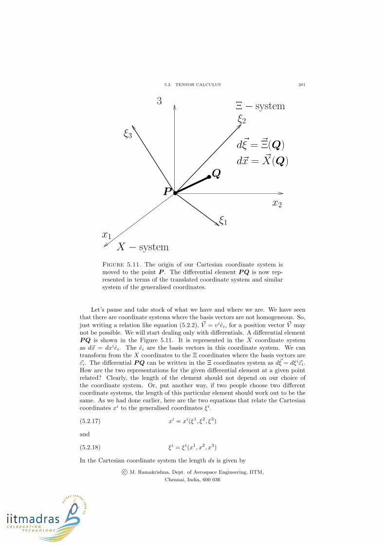
Figure 5.11. The origin of our Cartesian coordinate system ismoved to the point P . The differential element PQ is now rep-resented in terms of the translated coordinate system and similarsystem of the generalised coordinates.
Let’s pause and take stock of what we have and where we are. We have seenthat there are coordinate systems where the basis vectors are not homogeneous. So,
just writing a relation like equation (5.2.2), ~V = viei, for a position vector ~V maynot be possible. We will start dealing only with differentials. A differential elementPQ is shown in the Figure 5.11. It is represented in the X coordinate systemas d~x = dxiei. The ei are the basis vectors in this coordinate system. We cantransform from the X coordinates to the Ξ coordinates where the basis vectors are~εi. The differential PQ can be written in the Ξ coordinates system as d~ξ = dξi~εi.How are the two representations for the given differential element at a given pointrelated? Clearly, the length of the element should not depend on our choice ofthe coordinate system. Or, put another way, if two people choose two differentcoordinate systems, the length of this particular element should work out to be thesame. As we had done earlier, here are the two equations that relate the Cartesiancoordinates xi to the generalised coordinates ξi.
(5.2.17) xi = xi(ξ1, ξ2, ξ3)
and
(5.2.18) ξi = ξi(x1, x2, x3)
In the Cartesian coordinate system the length ds is given by
c© M. Ramakrishna, Dept. of Aerospace Engineering, IITM,
Chennai, India, 600 036
202 CHAPTER 5. TENSORS AND THE EQUATIONS OF FLUID MOTION
(5.2.19) (ds)2 = d~x · d~x = dxiei · dxj ej = dxidxj ei · ej
Remember that ei are the basis vectors of a Cartesian coordinate system and areorthogonal to each other. Consequently, we can define a useful entity called theKronecker delta as
(5.2.20) δij = ei · ej =
{1, i = j0, i 6= j
With this new notation we can write
(5.2.21) (ds)2 = d~x · d~x = dxidxjδij = dxidxi =∑
i
(dxi)2
Following the convention we have used so far ( without actually mentioning it ) wesee that
(5.2.22) dxjδij = dxi
That is, j is a dummy index and disappears leaving i which is a subscript. For thefirst time we have seen a contravariant quantity converted to a covariant quantity.If you think of matrix algebra for a minute, you will see that δij is like an identitymatrix. The components dxi are the same as the components dxi in a Cartesiancoordinate system. Hence, equation (5.2.21) can be written as
(5.2.23) (ds)2 = dxidxi =∑
i
(dxi)2
The length of the element is invariant with transformation meaning the choice ofour coordinates should not change the length of the element. A change to the Ξcoordinates should give us the same length for the differential element PQ. Thelength in the Ξ coordinates is given by
(5.2.24) (ds)2 = d~ξ · d~ξ = dξi~εi · dξj~εj = dξidξj~εi · ~εj = dξidξjgij = dξidξi
gij is called the metric. Following equation (5.2.22), we have defined dξi = gijdξj .
Why did we get gij instead of δij? We have seen in the case of the trapezium thatthe basis vectors need not be orthogonal to each other since the coordinate linesare not orthogonal to each other. So, the dot product of the basis vectors ~εi and~εj gives us a gij with non-zero off-diagonal terms. It is still symmetric, though. Inthis case, unlike the Cartesian situation, dξi is different from dξi.
We can define another set of basis vectors which are orthogonal to the covariantset as follows
(5.2.25) ~εi · ~εj = δj
i
where,
(5.2.26) δji =
{1, i = j0, i 6= j
This new basis, ~ε i, is called the contravariant basis or a dual basis. This isdemonstrated graphically in figure 5.12. This basis can be used to define a metric
(5.2.27) gij = ~ε i · ~ε j
c© M. Ramakrishna, Dept. of Aerospace Engineering, IITM,
Chennai, India, 600 036
5.2. TENSOR CALCULUS 203
~ε2
~ε1
~ε 3
~ε3
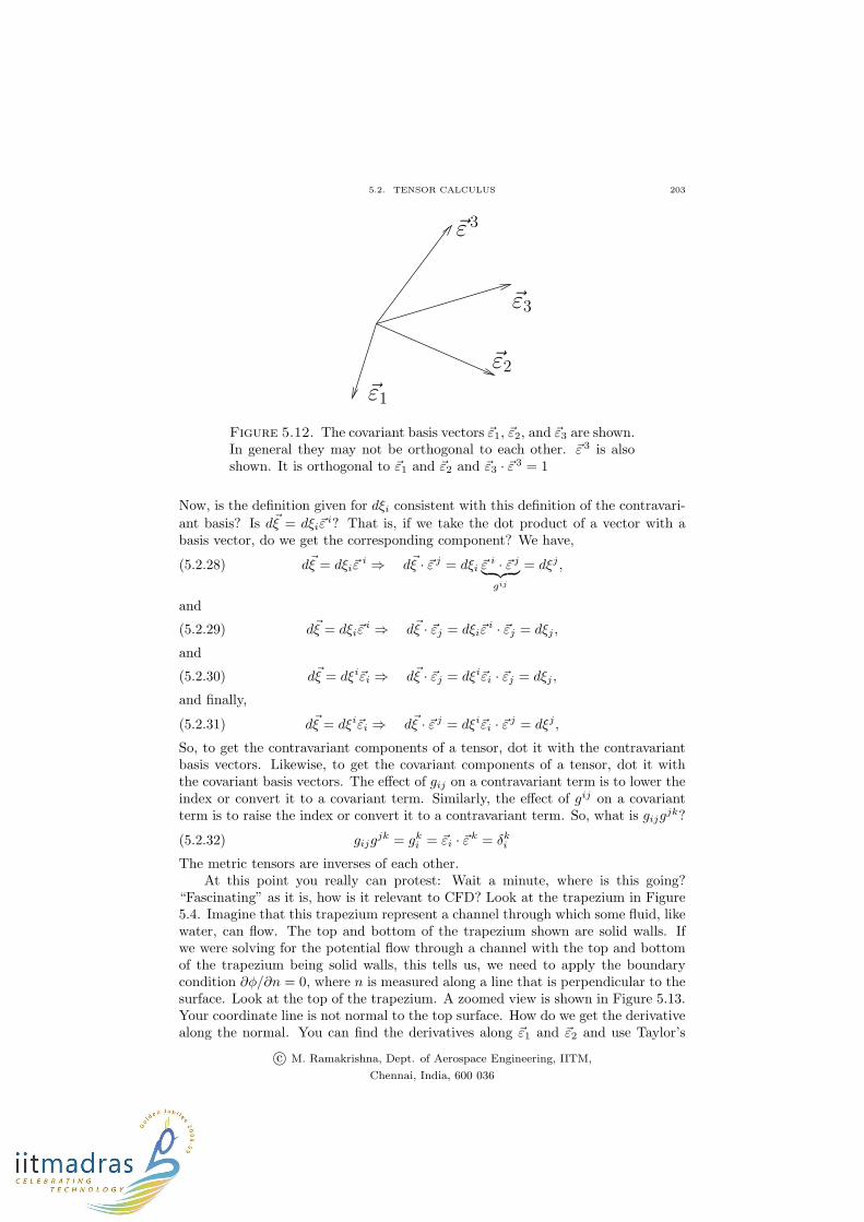
Figure 5.12. The covariant basis vectors ~ε1, ~ε2, and ~ε3 are shown.In general they may not be orthogonal to each other. ~ε 3 is alsoshown. It is orthogonal to ~ε1 and ~ε2 and ~ε3 · ~ε
3 = 1
Now, is the definition given for dξi consistent with this definition of the contravari-
ant basis? Is d~ξ = dξi~εi? That is, if we take the dot product of a vector with a
basis vector, do we get the corresponding component? We have,
(5.2.28) d~ξ = dξi~εi ⇒ d~ξ · ~ε j = dξi ~ε
i · ~ε j
︸ ︷︷ ︸
gij
= dξj ,
and
(5.2.29) d~ξ = dξi~εi ⇒ d~ξ · ~εj = dξi~ε
i · ~εj = dξj ,
and
(5.2.30) d~ξ = dξi~εi ⇒ d~ξ · ~εj = dξi~εi · ~εj = dξj ,
and finally,
(5.2.31) d~ξ = dξi~εi ⇒ d~ξ · ~ε j = dξi~εi · ~εj = dξj ,
So, to get the contravariant components of a tensor, dot it with the contravariantbasis vectors. Likewise, to get the covariant components of a tensor, dot it withthe covariant basis vectors. The effect of gij on a contravariant term is to lower theindex or convert it to a covariant term. Similarly, the effect of gij on a covariantterm is to raise the index or convert it to a contravariant term. So, what is gijg
jk?
(5.2.32) gijgjk = gk
i = ~εi · ~εk = δk
i
The metric tensors are inverses of each other.At this point you really can protest: Wait a minute, where is this going?
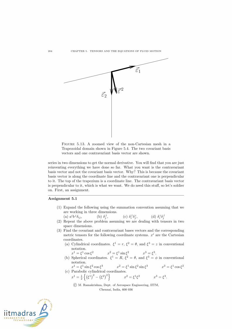
“Fascinating” as it is, how is it relevant to CFD? Look at the trapezium in Figure5.4. Imagine that this trapezium represent a channel through which some fluid, likewater, can flow. The top and bottom of the trapezium shown are solid walls. Ifwe were solving for the potential flow through a channel with the top and bottomof the trapezium being solid walls, this tells us, we need to apply the boundarycondition ∂φ/∂n = 0, where n is measured along a line that is perpendicular to thesurface. Look at the top of the trapezium. A zoomed view is shown in Figure 5.13.Your coordinate line is not normal to the top surface. How do we get the derivativealong the normal. You can find the derivatives along ~ε1 and ~ε2 and use Taylor’s
c© M. Ramakrishna, Dept. of Aerospace Engineering, IITM,
Chennai, India, 600 036
204 CHAPTER 5. TENSORS AND THE EQUATIONS OF FLUID MOTION
~ε1
~ε2
~ε 2
Figure 5.13. A zoomed view of the non-Cartesian mesh in aTrapezoidal domain shown in Figure 5.4. The two covariant basisvectors and one contravariant basis vector are shown.
series in two dimensions to get the normal derivative. You will find that you are justreinventing everything we have done so far. What you want is the contravariantbasis vector and not the covariant basis vector. Why? This is because the covariantbasis vector is along the coordinate line and the contravariant one is perpendicularto it. The top of the trapezium is a coordinate line. The contravariant basis vectoris perpendicular to it, which is what we want. We do need this stuff, so let’s soldieron. First, an assignment.
Assignment 5.1
(1) Expand the following using the summation convention assuming that weare working in three dimensions.(a) aib jδij , (b) δ j
j , (c) δ ji δ
ij , (d) δ i
i δjj
(2) Repeat the above problem assuming we are dealing with tensors in twospace dimensions.
(3) Find the covariant and contravariant bases vectors and the correspondingmetric tensors for the following coordinate systems. xi are the Cartesiancoordinates.(a) Cylindrical coordinates. ξ1 = r, ξ2 = θ, and ξ3 = z in conventional
notation.x1 = ξ1 cos ξ2 x2 = ξ1 sin ξ2 x3 = ξ3.
(b) Spherical coordinates. ξ1 = R, ξ2 = θ, and ξ3 = φ in conventionalnotation.x1 = ξ1 sin ξ2 cos ξ3 x2 = ξ1 sin ξ2 sin ξ3 x3 = ξ1 cos ξ2
(c) Parabolic cylindrical coordinates.
x1 = 12
{(ξ1
)2−
(ξ2
)2}
x2 = ξ1ξ2 x3 = ξ3.
c© M. Ramakrishna, Dept. of Aerospace Engineering, IITM,
Chennai, India, 600 036
5.2. TENSOR CALCULUS 205
(4) Compute the covariant and contravariant velocity components in the abovecoordinate systems.
You have seen in multivariate calculus that given a smooth function φ, in aregion of interest, we can find the differential dφ as
(5.2.33) dφ =∂φ
∂ξidξi
Now, we also know that this is a directional derivative and can be written as
(5.2.34) dφ = ∇φ · d~ξ =∂φ
∂ξidξi
where,
(5.2.35) ∇ = ~ε j ∂
∂ξj, d~ξ = ~εidξ
i
We managed to define the gradient operator ∇. What happens when we take thegradient of a vector? How about the divergence? We first write the gradients of ascalar function and a vector function as
∇φ = ~ε j ∂φ
∂ξj(5.2.36)
∇~V = ~ε j ∂~V
∂ξj(5.2.37)
If we look carefully at the two equation above, we see that equation (5.2.37) isdifferent. It involves, due to the use of product rule, the derivatives of the basisvectors. In fact, equation (5.2.37) can written as
(5.2.38) ∇~V = ~ε j ∂~V
∂ξj= ~ε j
{∂vi
∂ξj~εi + vi ∂~εi
∂ξj
}
So, what is the nature of the derivative of the basis vector? For one thing, fromthe definition of the covariant basis in equation (5.2.12) we have
(5.2.39)∂~εi
∂ξ j=
∂2~α
∂ξj∂ξi=∂~εj
∂ξi
We have dispensed with the subscript on ~α so as not to create more confusion.We will use the correct ~α corresponding to the coordinate line. We can see fromequation (5.2.39) that its component representation is going to be symmetric inthe two indices i and j. As we have already seen in equation (5.2.28), to find thecontravariant components of this entity we can dot it with ~ε k to get
(5.2.40)
{kij
}
= ~ε k ·∂~εi
∂ξj
{kij
}is called a Christoffel symbol of the second kind. We took the dot product
with ~ε k so that equation (5.2.38) can be rewritten as
(5.2.41) ∇~V = ~ε j
{∂vi
∂ξj~εi + vi
{kij
}
~εk
}
c© M. Ramakrishna, Dept. of Aerospace Engineering, IITM,
Chennai, India, 600 036
206 CHAPTER 5. TENSORS AND THE EQUATIONS OF FLUID MOTION
Since i and k are dummy indices (meaning we are going to sum over their values)we swap them for a more convenient expression
(5.2.42) ∇~V = ~ε j
{∂vi
∂ξj~εi + vk
{ikj
}
~εi
}
This allows us to write
(5.2.43)∂~V
∂ξj=
{∂vi
∂ξj+ vk
{ikj
}}
~εi
In pure component form this is written as
(5.2.44) vi;j =
∂vi
∂ξj+ vk
{ikj
}
This is called the covariant derivative of the contravariant vector vi. Staying withour compact notation, the covariant derivative is indicated by the semi-colon in thesubscript. This is so that we do not confuse it with the plain derivative ∂vi/∂ξj .
So, if we have Christoffel symbols of the second kind do we have any otherkind? Yes, there is a Christoffel symbol of the first kind. It is written as [ij, k] andit is given by
(5.2.45) [ij, k] =
{lij
}
glk =∂~εi
∂ξj· ~ε lglk =
∂~εi
∂ξj· ~εk
The Christoffel symbols of the first kind can be directly obtained as
(5.2.46) [ij, k] =1
2
(∂gjk
∂ξi+∂gki
∂ξj−∂gij
∂ξk
)
This can be verified by substituting for the definition of the metric tensor. Thepeculiar notation with brackets and braces is used for the Christoffel symbols (andthey are called symbols) because, it turns out that they are not tensors. That is,though they have indices, they do not transform the way tensors do when going fromone coordinate system to another. We are not going to show this here. However,we should not be surprised that they are not tensors as the Christoffel symbolsencapsulate the relationship of the two coordinate systems and would necessarilydepend on the coordinates.
The divergence of ~V is defined as the trace of the gradient of ~V . That is
(5.2.47) div~V = ~ε j ·
{∂vi
∂ξj~εi + vk
{ikj
}
~εi
}
Assignment 5.2
For the coordinate systems given in assignment 5.1,
(1) Find the Christoffel symbols of the first and second kind.(2) Find the expression for the gradient of a scalar potential.(3) Find the gradient of the velocity vector.(4) Find the divergence of the velocity vector.(5) Find the divergence of the gradient of the scalar potential that you just
found.
c© M. Ramakrishna, Dept. of Aerospace Engineering, IITM,
Chennai, India, 600 036

5.3. EQUATIONS OF FLUID MOTION 207
In the case of the velocity potential ~V = ∇φ we get,
(5.2.48) ~V = ~ε j ∂φ
∂ξj= ~εkg
kj ∂φ
∂ξj= ~εkg
kjvj = vk~εk
If we now take the divergence of this vector using equation (5.2.47) we get(5.2.49)
∇2φ = ~ε j ·
{∂vi
∂ξj~εi + vk
{ikj
}
~εi
}
= ~ε j ·
{∂
∂ξj
(
gil ∂φ
∂ξl
)
~εi + vk
{ikj
}
~εi
}
Completing the dot product we get
(5.2.50) ∇2φ =
{∂
∂ξi
(
gil ∂φ
∂ξl
)
+ vk
{iki
}}
Substituting for vk from equation (5.2.48) we get
(5.2.51) ∇2φ =
{∂
∂ξi
(
gil ∂φ
∂ξl
)
+ gkl ∂φ
∂ξl
{iki
}}
This much tensor calculus will suffice. A more in depth study can be madeusing the numerous books that are available on the topic [You93], [SS82].
5.3. Equations of Fluid Motion
We have seen enough tensor calculus so that if we derive the governing equationsin some generic coordinate system, we can always transform the resulting equationsinto any other coordinate system. In fact, as far as possible, we will derive theequations in vector form so that we can pick the component form that we feel isappropriate for us. We can conveniently use the Cartesian coordinate system forthe derivation with out loss of generality.
We will first derive the equations of motion in integral form. We will do this ina general setting. Let us consider some fluid property Q, whose property densityis given by Q. For example, consider a situation in which we have added some inkto flowing water. At any given time, the mass of ink in a small elemental region ofinterest may be dmink. If the volume of the elemental region is dσ, then these twomeasures defined on that region are related through the ink density as
(5.3.1) dmink =dmink
dσdσ = ρinkdσ
We would like to write out the balance laws for a general property, Q. Wearbitrarily pick a control volume. One such volume is indicated in the Figure5.14. For the sake of simplicity, we pick a control volume that does not change intime. This control volume occupies a region of volume σ. This control volume hasa surface area S. It is located as shown in the figure and is immersed in a flow field.Within this control volume, at an arbitrary point ~x, we pick a small elementalregion with volume dσ. From equation (5.3.1), the amount of the property ofinterest at time t, dQ(~x, t), in the elemental control volume is Q(~x, t)dσ. Then thetotal quantity contained in our control volume at any instant is
(5.3.2) Qσ(t) =
∫
σ
Q(~x, t)dσ
c© M. Ramakrishna, Dept. of Aerospace Engineering, IITM,
Chennai, India, 600 036
208 CHAPTER 5. TENSORS AND THE EQUATIONS OF FLUID MOTION
dS
dσ
2
3
1
~x
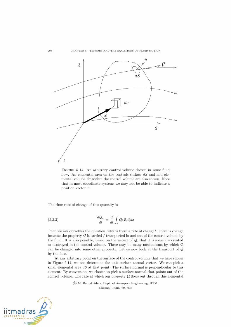
n~V
Figure 5.14. An arbitrary control volume chosen in some fluidflow. An elemental area on the controls surface dS and and ele-mental volume dσ within the control volume are also shown. Notethat in most coordinate systems we may not be able to indicate aposition vector ~x.
The time rate of change of this quantity is
(5.3.3)dQσ
dt=
d
dt
∫
σ
Q(~x, t)dσ
Then we ask ourselves the question, why is there a rate of change? There is changebecause the property Q is carried / transported in and out of the control volume bythe fluid. It is also possible, based on the nature of Q, that it is somehow createdor destroyed in the control volume. There may be many mechanisms by which Q
can be changed into some other property. Let us now look at the transport of Qby the flow.
At any arbitrary point on the surface of the control volume that we have shownin Figure 5.14, we can determine the unit surface normal vector. We can pick asmall elemental area dS at that point. The surface normal is perpendicular to thiselement. By convention, we choose to pick a surface normal that points out of thecontrol volume. The rate at which our property Q flows out through this elemental
c© M. Ramakrishna, Dept. of Aerospace Engineering, IITM,
Chennai, India, 600 036
5.3. EQUATIONS OF FLUID MOTION 209
area is given by Q~V · ndS. The total efflux (outflow) from the control volume is
(5.3.4)
∫
S
Q~V · ndS
Since this is a net efflux, it would cause a decrease in the amount of Q containedin the control volume. So, our balance law can be written as
(5.3.5)d
dt
∫
σ
Qdσ = −
∫
S
Q~V · ndS + any other mechanism to produce Q
Before going on we will make the following observation. Though the control volumecan be picked arbitrarily, we will make sure that it is smooth enough to have surfacenormals almost everywhere. Almost everywhere? If you think of a cube, we cannotdefine surface normals at the edges and corners. We can break up the surfaceintegral in equation (5.3.5) into the sum of six integrals, one for each face of thecube.
5.3.1. Conservation of Mass. Let us look at an example. If the propertywe were considering was mass, Qσ(t) would be the mass of fluid in our controlvolume at any given time. The corresponding Q would be mass density which weroutinely refer to as the density, ρ. Ignoring mechanisms to create and destroy orotherwise modify mass, we see that the production terms disappear, leaving onlythe first term on the right hand side of equation (5.3.5). This gives us the equationfor balance of mass as
(5.3.6)d
dt
∫
σ
ρdσ = −
∫
S
ρ~V · ndS
This equation is also called the conservation of mass equation.
5.3.2. Conservation of Linear Momentum. On the other hand, if we con-
sider the property Q to be momentum, the property density Q turns out to be ρ~V ,which is the momentum density. In this case, we know that the total momentumin the control volume can also be changed by applying forces. For the sake of thisdiscussion, forces come in two flavours. There are those that correspond to actionacross a distance, these forces are often called body forces. The others that dependon proximity are called surface forces1. We can write our equation of balance of
linear momentum as
(5.3.7)d
dt
∫
σ
ρ~V dσ = −
∫
S
ρ~V ~V · ndS +
∫
σ
~fdσ +
∫
S
~TdS
Here, ~f(~x) is the body force per unit volume at the point ~x within the control
volume. ~T (~x) is the traction force per unit area acting at some point ~x on thecontrol surface. If we are willing or able to ignore the body force, we are left withthe traction force to be handled. From fluid mechanics, you would have seen thatwe can associate at a point, a linear transformation called the stress tensor, whichrelates the normal to a surface element to the traction force on that element. Thatis
(5.3.8) ~T = τ · n
1 As with everything that we do in physics, what we mean by this really depends on length
scales. We have assumed that we are dealing with a continuum and that implicitly has a bifurcation
of the length scales built into it.
c© M. Ramakrishna, Dept. of Aerospace Engineering, IITM,
Chennai, India, 600 036
210 CHAPTER 5. TENSORS AND THE EQUATIONS OF FLUID MOTION
where, ~T = Ti~εi, τ = τij~ε
i~ε j , and n = nk~εk. This gives us the Cauchy equation
in component form as
(5.3.9) Ti = τijnj
The momentum balance equation can be written as
(5.3.10)d
dt
∫
σ
ρ~V dσ = −
∫
S
ρ~V ~V · ndS +
∫
S
τ · ndS
Combining terms we get
(5.3.11)d
dt
∫
σ
ρ~V dσ = −
∫
S
{
ρ~V ~V − τ}
· ndS
5.3.3. Conservation of Energy. Finally, if we consider the total energy asthe property of interest so that we write out the balance law for energy. Consideringthe form of the first two equations, we will define the total energy density as ρEt,where Et is the specific total energy defined as
(5.3.12) Et = e+1
2~V · ~V ,
Where e is the specific internal energy defined for a perfect gas as e = CvT . Cv
is the specific heat at constant volume and T is the temperature measured on theKelvin scale. We need to look at the production terms again in equation (5.3.5).The total energy in our control volume can be changed by
(1) the forces from the earlier discussion doing work on the control volume,(2) the transfer of energy by the process of heat through radiation and con-
duction,(3) the apparent creation of energy through exo-thermic or endo-thermic
chemical reactions,(4) and finally, of course, the transportation of energy across the control sur-
face by the fluid.
We will ignore radiation and chemical reactions here. This results in the balancelaw
(5.3.13)d
dt
∫
σ
ρEtdσ = −
∫
S
ρEt~V · ndS +
∫
σ
~f · ~V dσ +
∫
S
~T · ~V dS −
∫
S
~q · ndS
Here, ~q is the term quantifying heat. Again, if we are in a position to ignore bodyforces we get
(5.3.14)d
dt
∫
σ
ρEtdσ = −
∫
S
ρEt~V · ndS +
∫
S
~V · τ · ndS −
∫
S
~q · ndS
which we conveniently rewrite incorporating the other balance laws as
(5.3.15)d
dt
∫
σ
Qdσ = −
∫
S
~F · ndS
where we have
(5.3.16) Q =
ρ
ρ~VρEt
, ~F =
ρ~V
ρ~V ~V − τ
(ρEt)~V − τ · ~V + ~q
where, τ · ~V is the rate at which the traction force does work on the control volume.This, gives us a consolidated statement for the balance (conservation) of mass,
c© M. Ramakrishna, Dept. of Aerospace Engineering, IITM,
Chennai, India, 600 036
5.3. EQUATIONS OF FLUID MOTION 211
linear momentum, and energy. The great thing about this equation is that it canbe cast in any three dimensional coordinate system to get the component form. Itis written in a coordinate free fashion. Though, it is good to admire, we finallyneed to solve a specific problem, so we pick a coordinate system convenient for thesolution of our problem and express these equations in that coordinate system. Theother problem is that as it is there is some element of ambiguity in the dot products
of the form (τ · ~V ) · n. These ambiguities are best resolved in terms of components.
(5.3.17) ~T · ~V = Ti~εi · ~εlV
l = τij~εi(~ε j · ~ε k)nk · ~εlV
l = τijnjV i
The differential form of equation (5.3.15) can be obtained by applying the theoremof Gauss to the right hand side of the equation and converting the surface integralto a volume integral.
(5.3.18)
∫
σ
{∂Q
∂t+ div ~F
}
dσ = 0
The control volume is chosen arbitrarily. As a consequence, the integral needs tobe zero for any σ over which we integrate. This is possible only if
(5.3.19)∂Q
∂t+ div ~F = 0
The form of equation (5.3.15) is quite general. We could add, as required, more
terms to the ~F on the right hand side. We could also add as many equations asrequired. If you have other properties that need to be tracked, the correspondingequations can be incorporated. However, for our purpose, these equations are quitegeneral. We will start with a little specialisation and simplification.
We now decompose the stress tensor τ into a spherical part and a deviatoricpart. The spherical part we will assume is the same as the pressure we have in theequation of state. The deviatoric part [ or the deviation from the sphere ] will showup due to viscous effects. So, τ can be written as
(5.3.20) τ = −p1 + σ
1 is the unit tensor and σ is the deviatoric part. Do not confuse σ a tensor withthe control volume σ. Through thermodynamics, we have an equation of state /constitutive model for p. Typically, we use something like p = ρRT , where T is thetemperature in Kelvin and R is the gas constant. We need to get a similar equationof state / constitutive model for σ. Assuming the fluid is a Navier-Stokes fluid,that is the fluid is Newtonian, isotropic and Stokes hypothesis holds we get
σ = −2
3µtrD + 2µD, where(5.3.21)
D =1
2(L + LT ), and(5.3.22)
L = ∇~V(5.3.23)
where µ is the coefficient of viscosity and trD is the trace of D. Which is the sumof the diagonals of the matrix representation of the tensor. LT is the transpose of
L. Really, D is the symmetric part of the the gradient of ~V . Since we are rightnow looking at inviscid flow, we can ignore the viscous terms. So, for the Euler’sequation we have
(5.3.24) ~T = −p1 · n
c© M. Ramakrishna, Dept. of Aerospace Engineering, IITM,
Chennai, India, 600 036
212 CHAPTER 5. TENSORS AND THE EQUATIONS OF FLUID MOTION
where, 1 is the unit tensor. The Euler’s momentum conservation equation can bewritten as
(5.3.25)d
dt
∫
σ
ρ~V dσ = −
∫
S
ρ~V ~V · ndS −
∫
S
p1 · ndS
Combining terms we get
(5.3.26)d
dt
∫
σ
ρ~V dσ = −
∫
S
{
ρ~V ~V + p1}
· ndS
which we conveniently rewrite as
(5.3.27)d
dt
∫
σ
Qdσ = −
∫
S
~F · ndS
where we have
(5.3.28) Q =
ρ
ρ~VρEt
, ~F =
ρ~V
ρ~V ~V + p1
(ρEt + p)~V
giving us a consolidated statement for the conservation [ or balance ] of mass, linearmomentum, and energy. These equations are collectively referred to as the Euler’sequation. There are, as is usual, a set of auxiliary equations to complement theseequations. The constitutive model given by the equation of state is
(5.3.29) p = ρRT
and
(5.3.30) Et = e+~V · ~V
2
(5.3.31) e = CvT
With these added equations we have a closed set of equations that we shouldbe able to solve. The equations are in integral form. We can employ the theoremof Gauss on the surface integral in equation (5.3.27) and convert it to a volumeintegral like so
(5.3.32)d
dt
∫
σ
Qdσ = −
∫
S
~F · ndS = −
∫
σ
div ~Fdσ
This gives us the following equation
(5.3.33)
∫
σ
(∂Q
∂t+ div ~F
)
dσ = 0
which is valid for all possible control volumes on which we have surface normalsand can perform the necessary integration. Remember, this “particular” σ waschosen arbitrarily. We conclude that the integral can be zero for any σ only if theintegrand is zero. The differential form of the Euler’s equation can be written as
(5.3.34)∂Q
∂t+ div ~F = 0
If we use normal convention to write ~F in Cartesian coordinates as
(5.3.35) ~F = Eı+ F +Gk
c© M. Ramakrishna, Dept. of Aerospace Engineering, IITM,
Chennai, India, 600 036
5.3. EQUATIONS OF FLUID MOTION 213
our governing equation in Cartesian coordinates then becomes
(5.3.36)∂Q
∂t+∂E
∂x+∂F
∂y+∂G
∂z= 0
Clearly, given any other basis vector, metrics, Christoffel symbols, we can write thegoverning equations in the corresponding coordinate system.
Assignment 5.3
(1) Given the concentration of ink at any point in a flow field is given by ci,derive the conservation equation in integral form for ink. The diffusivityof ink is Di.
(2) From the integral from in the first problem, derive the differential form(3) Specialise the equation for a two-dimensional problem.(4) Derive the equation in polar coordinates.
5.3.4. Non-dimensional Form of Equations. So far, in this book, we havenot talked of the physical units used. How do the equations depend on physical unitsthat we use. Does the solution depend on the fact that we use millimetres insteadof metres? We would like to solve the non-dimensional form of these equations. Wewill demonstrate the process of obtain the non-dimensional form of the equationusing the two-dimensional Euler’s equation written in Cartesian coordinates.
(5.3.37)∂Q
∂t+∂E
∂x+∂F
∂y= 0
To this end, we define the following reference parameters and relationships.It should be noted that the whole aim of this choice is to retain the form of theequations.
We have a characteristic length L in the problem that we will use to scalelengths and coordinates. For example
(5.3.38) x∗ =x
L, and y∗ =
y
L
We employ a reference density ρr and a reference pressure pr to non-dimensionlisethe density and the pressure. As a result we get the non-dimensionalisation for thetemperature through the equation of state.(5.3.39)
ρ∗ =ρ
ρr
, and p∗ =p
pr
, along with p = ρRT gives T ∗ =T
Tr
,
where,
(5.3.40) Tr =pr
ρrR,
and the equation of state reduces to
(5.3.41) p∗ = ρ∗T ∗
Consider the one-dimensional energy equation from gas dynamics. This relationtells us that
c© M. Ramakrishna, Dept. of Aerospace Engineering, IITM,
Chennai, India, 600 036
214 CHAPTER 5. TENSORS AND THE EQUATIONS OF FLUID MOTION
(5.3.42) CpTo = CpT +V 2
2
If we divide this equation through by Tr and nondimensionalise speed with areference speed ur we get
(5.3.43) CpT∗
o = CPT∗ +
V ∗2u2r
2Tr
Now we see that if we define
(5.3.44) ur =√
RTr
equation (5.3.43) reduces to
(5.3.45)γ
γ − 1T ∗
o =γ
γ − 1T ∗ +
V ∗2
2
Now, consider the first equation, conservation of mass, from equations (5.3.37).This becomes
(5.3.46)ρr
τ
∂ρ∗
∂t∗+ρrur
L
∂ρ∗u∗
∂x∗+ρrur
L
∂ρ∗v∗
∂y∗= 0
where τ is some characteristic time scale to be defined here. Dividing through byρrur and multiplying through by L, we get
(5.3.47)L
urτ
∂ρ∗
∂t∗+∂ρ∗u∗
∂x∗+∂ρ∗v∗
∂y∗= 0
Clearly, if we define the time scale τ = L/ur we get back our original equation.I will leave it as an exercise in calculus for the student to show that given thefollowing summary
x∗ =x
L, and y∗ =
y
L(5.3.48)
ρ∗ =ρ
ρr
, and p∗ =p
pr
,(5.3.49)
Tr =pr
ρrR, and ur =
√
RTr(5.3.50)
equation (5.3.37) reduces to
(5.3.51)∂Q∗
∂t∗+∂E∗
∂x∗+∂F ∗
∂y∗= 0
where
(5.3.52)
Q∗ =
ρ∗
ρ∗u∗
ρ∗v∗
ρ∗E∗
t
, E∗ =
ρ∗u∗
ρ∗u∗2 + p∗
ρ∗u∗v∗
(ρ∗E∗
t + p∗)u∗
, and F ∗ =
ρ∗v∗
ρ∗u∗v∗
ρ∗v∗2 + p∗
(ρ∗E∗
t + p∗)v∗
c© M. Ramakrishna, Dept. of Aerospace Engineering, IITM,
Chennai, India, 600 036
5.3. EQUATIONS OF FLUID MOTION 215
Very often for the sake of convenience the “stars” are dropped. One has toremember that though these basic equations have not changed form. Others havechanged form. The equation of state becomes p∗ = ρ∗T ∗ and the energy equationchanges form. Any other auxiliary equation that you may use has to be nondimen-sionalised using the same reference quantities.
A careful study will show you that if L, pr and ρr are specified then all the otherreference quantities can be derived. In fact, we typically need to fix two referencequantities along with a length scale and the others can be determined. The otherpoint to note is that we typically pick reference quantities based on the problem athand. A review of dimensional analysis at this point would be helpful.
Assignment 5.4
(1) Non-dimensionalise the Euler’s equation in the differential form for three-dimensional flows.
(2) Try to non-dimensionalise the Burgers’ equation
(5.3.53)∂u
∂t+ u
∂u
∂x= ν
∂2u
∂x2
u does not have the units of speed.
c© M. Ramakrishna, Dept. of Aerospace Engineering, IITM,
Chennai, India, 600 036