Embed Size (px)
Citation preview

Chapter 3
Governing Equations of FluidDynamics
The starting point of any numerical simulation are the governing equations of the physics of theproblem to be solved. In this chapter, we first present the governing equations of fluid dynamicsand their nondimensionalization. Then, we describe their transformation to generalized curvilin-ear coordinates. And finally, we close this chapter by presenting the governing equations for thecase of an incompressible viscous flow.
3.1 Navier-Stokes System of Equations
The equations governing the motion of a fluid can be derived from the statements of the conserva-tion of mass, momentum, and energy [5]. In the most general form, the fluid motion is governedby the time-dependent three-dimensional compressible Navier-Stokes system of equations. Fora viscous Newtonian, isotropic fluid in the absence of external forces, mass di!usion, finite-ratechemical reactions, and external heat addition, the strong conservation form of the Navier-Stokessystem of equations in compact di!erential form can be written as
!"
!t+! · ("u) = 0
! ("u)!t
+! · ("uu) = "!p +! · #
! ("et)!t
+! · ("etu) = k! ·! T "!p · u + (! · #) · u
This set of equations can be rewritten in vector form as follows
!Q!t
+!Ei
!x+
!Fi
!y+
!Gi
!z=
!Ev
!x+
!Fv
!y+
!Gv
!z(3.1)
where Q is the vector of the conserved flow variables given by
34
3.1. NAVIER-STOKES SYSTEM OF EQUATIONS
Q =
!
""""#
""u"v"w"et
$
%%%%&(3.2)
and Ei = Ei(Q), Fi = Fi(Q) and Gi = Gi(Q) are the vectors containing the inviscid fluxes inthe x, y and z directions and are given by
Ei =
!
""""#
"u"u2 + p
"uv"uw
("et + p) u
$
%%%%&, Fi =
!
""""#
"v"vu
"v2 + p"vw
("et + p) v
$
%%%%&, Gi =
!
""""#
"w"wu"wv
"w2 + p("et + p)w
$
%%%%&(3.3)
where u is the velocity vector containing the u, v and w velocity components in the x, y and zdirections and p, " and et are the pressure, density and total energy per unit mass respectively.
The vectors Ev = Ev(Q), Fv = Fv(Q) and Gv = Gv(Q) contain the viscous fluxes in the x, yand z directions and are defined as follows
Ev =
!
""""#
0#xx
#xy
#xz
u#xx + v#xy + w#xz " qx
$
%%%%&
Fv =
!
""""#
0#yx
#yy
#yz
u#yx + v#yy + w#yz " qy
$
%%%%&
Gv =
!
""""#
0#zx
#zy
#zz
u#zx + v#zy + w#zz " qz
$
%%%%&
(3.4)
where the heat fluxes qx, qy and qz are given by the Fourier’s law of heat conduction as follows
qx = "k!T
!x
qy = "k!T
!y
qz = "k!T
!z
(3.5)
and the viscous stresses #xx, #yy, #zz, #xy, #yx, #xz, #zx, #yz and #zy, are given by the following
35
CHAPTER 3. GOVERNING EQUATIONS OF FLUID DYNAMICS
relationships
#xx =23µ
'2!u
!x" !v
!y" !w
!z
(
#yy =23µ
'2!v
!y" !u
!x" !w
!z
(
#zz =23µ
'2!w
!z" !u
!x" !v
!y
(
#xy = µ
'!u
!y+
!v
!x
(
#xz = µ
'!u
!z+
!w
!x
(
#yz = µ
'!v
!z+
!w
!y
(
#yx = #xy
#zx = #xz
#zy = #yz
(3.6)
where µ is the laminar viscosity.
Examining closely equations eq. 3.1, eq. 3.2, eq. 3.3 and eq. 3.4 and counting the number ofequations and unknowns, we clearly see that we have five equations in terms of seven unknownflow field variables u, v, w, ", p, T , and et. It is obvious that two additional equations arerequired to close the system. These two additional equations can be obtained by determiningrelationships that exist between the thermodynamic variables (p, ", T, ei) through the assumptionof thermodynamic equilibrium. Relations of this type are known as equations of state, andthey provide a mathematical relationship between two or more state functions (thermodynamicvariables). Choosing the specific internal energy ei and the density " as the two independentthermodynamic variables, then equations of state of the form
p = p (ei, ") , T = T (ei, ") (3.7)
are required.
For most problems in aerodynamics and gasdynamics, it is generally reasonable to assume thatthe gas behaves as a perfect gas (a perfect gas is defined as a gas whose intermolecular forces arenegligible), i.e.,
p = "RgT (3.8)
where Rg is the specific gas constant and is equal to 287 m2
s2K for air. Assuming also that theworking gas behaves as a calorically perfect gas (a calorically perfect gas is defined as a perfectgas with constant specific heats), then the following relations hold
ei = cvT, h = cpT, $ =cp
cv, cv =
Rg
$ " 1, cp =
$Rg
$ " 1(3.9)
36

3.2. NONDIMENSIONALIZATION OF THE GOVERNING EQUATIONS
where $ is the ratio of specific heats and is equal to 1.4 for air, cv the specific heat at constantvolume, cp the specific heat at constant pressure and h is the enthalpy. By using eq. 3.8 andeq. 3.9, we obtain the following relations for pressure p and temperature T in the form of eq. 3.7
p = ($ " 1) "ei, T =p
"Rg=
($ " 1) ei
Rg(3.10)
where the specific internal energy per unit mass ei = p/($" 1)" is related to the total energy perunit mass et by the following relationship,
et = ei +12
)u2 + v2 + w2
*(3.11)
In our discussion, it is also necessary to relate the transport properties (µ, k) to the thermody-namic variables. Then, the laminar viscosity µ is computed using Sutherland’s formula
µ =C1T
32
(T + C2)(3.12)
where for the case of the air, the constants are C1 = 1.458# 10!6 kgms"
Kand C2 = 110.4K.
The thermal conductivity, k, of the fluid is determined from the Prandtl number (Pr = 0.72 for air)which in general is assumed to be constant and is equal to
k =cpµ
Pr(3.13)
where cp and µ are given by equations eq. 3.9 and eq. 3.12 respectively.
The first row in eq. 3.1 corresponds to the continuity equation. Likewise, the second, third andfourth rows are the momentum equations, while the fifth row is the energy equation in terms oftotal energy per unit mass.
The Navier-Stokes system of equations eq. 3.1, eq. 3.2, eq. 3.3 and eq. 3.4, is a coupled systemof nonlinear partial di!erential equations (PDE), and hence is very di"cult to solve analytically.There is no general closed-form solution to this system of equations; hence we look for an ap-proximate solution of this system of equation in a given domain D with prescribed boundaryconditions !D and given initial conditions DU.
If in eq. 3.1 we set the viscous fluxes Ev = 0, Fv = 0 and Gv = 0, we get the Euler system ofequations, which governs inviscid fluid flow. The Euler system of equations is a set of hyperbolicequations while the Navier-Stokes system of equations is a mixed set of hyperbolic (in the inviscidregion) and parabolic (in the viscous region) equations. Therefore, time marching algorithms areused to advance the solution in time using discrete time steps.
3.2 Nondimensionalization of the Governing Equations
The governing fluid dynamic equations shown previously may be nondimensionalized to achievecertain objectives. The advantage in doing this is that, firstly, it will provide conditions upon
37

CHAPTER 3. GOVERNING EQUATIONS OF FLUID DYNAMICS
which dynamic and energetic similarity may be obtained for geometrically similar situations.Secondly, by nondimensionalizing the equations appropriately, the flow variables are normalizedso that their values fall between certain prescribed limits such as zero and one. Thirdly, theprocedure of nondimensionalization, also allows the solution to be independent of any systemof units and helps to reduce the sensitivity of the numerical algorithm to round-o!-errors. Andfinally, by nondimensionalizing the governing equations, characteristic parameters such as Machnumber, Reynolds number and Prandtl number can be varied independently. Among manychoices, in external flow aerodynamics it is reasonable to normalize with respect to the freestreamparameters so that
x =x
L, y =
y
L, z =
z
L
u =u
U#, v =
v
U#, w =
w
U#
" ="
"#, T =
T
T#, p =
p
"#U2#
t =tU#L
, et =et
U2#
, µ =µ
µ#
(3.14)
where ˜ denotes nondimensional quantities, the subscript # denotes freestream conditions, L issome dimensional reference length (such as the chord of an airfoil or the length of a vehicle), andU# is the magnitude of the freestream velocity. The reference length L is used in defining thenondimensional Reynold’s number, this parameter represents the ratio of inertia forces to viscousforces, and is given by
ReL ="#U#L
µ#(3.15)
where the freestream laminar viscosity µ# is computed using the freestream temperature T#according to eq. 3.12.
When dealing with high speed compressible flow, it is also useful to introduce the Mach number.The Mach number is a nondimensional parameter that measures the speed of the gas motion inrelation to the speed of sound a,
a =+'
!p
!"
(
s
, 12
=-
$p
"=
.$RgT (3.16)
Then the Mach number M# is given by,
M# =U#a
=U#.$ (p/")
=U#.$RgT
(3.17)
Finally, the remaining nondimensional quantities are defined as follows
38

3.2. NONDIMENSIONALIZATION OF THE GOVERNING EQUATIONS
Rg =Rg
U2#/T#
=1
$M2#
cp =1
($ " 1) M2#
C1 = C1T 1/2#µ#
C2 =C2
T#
(3.18)
Now, by simple replacing into the governing equations eq. 3.1 the dimensional quantities by theircorresponding nondimensional equivalent, the following nondimensional equations are obtained
!Q! t
+!Ei
!x+
!Fi
!y+
!Gi
!z=
!Ev
!x+
!Fv
!y+
!Gv
!z(3.19)
where Q is the vector of the nondimensional conserved flow variables given by
Q =
!
""""#
""u"v"w"et
$
%%%%&(3.20)
and Ei = Ei˜(Q), Fi = Fi
˜(Q) and Gi = Gi˜(Q) are the vectors containing the nondimensional
inviscid fluxes in the x, y and z directions and are given by
Ei =
!
""""#
"u"u2 + p
"uv"uw
("et + p) u,
$
%%%%&, Fi =
!
""""#
"v"vu
"v2 + p"vw
("et + p) v,
$
%%%%&, Gi =
!
""""#
"w"wu"wv
"w2 + p("et + p) w
$
%%%%&(3.21)
and Ev = Ev˜(Q), Fv = Fv
˜(Q) and Gv = Gv˜(Q) are the vectors containing the nondimensional
viscous fluxes in the x, y and z directions and are given by
39

CHAPTER 3. GOVERNING EQUATIONS OF FLUID DYNAMICS
Ev =
!
""""#
0#xx
#xy
#xz
u#xx + v#xy + w#xz " qx
$
%%%%&
Fv =
!
""""#
0#yx
#yy
#yz
u#yx + v#yy + w#yz " qy
$
%%%%&
Gv =
!
""""#
0#zx
#zy
#zz
u#zx + v#zy + w#zz " qz
$
%%%%&
(3.22)
However, in the process of nondimensionalizing the equations, the terms M# and ReL arises fromthe nondimensional viscous flux vectors. Therefore, the definition of the heat flux componentsand the viscous stresses may be modified as follows
qx = " µ
($ " 1) M2#ReLPr
!T
!x
qy = " µ
($ " 1) M2#ReLPr
!T
!y
qz = " µ
($ " 1) M2#ReLPr
!T
!z
(3.23)
and
40
3.3. TRANSFORMATION OF THE GOVERNING EQUATIONS TOGENERALIZED CURVILINEAR COORDINATES
#xx =23
µ
ReL
'2!u
!x" !v
!y" !w
!z
(
#yy =23
µ
ReL
'2!v
!y" !u
!x" !w
!z
(
#zz =23
µ
ReL
'2!w
!z" !u
!x" !v
!y
(
#xy =µ
ReL
'!u
!y+
!v
!x
(
#xz =µ
ReL
'!u
!z+
!w
!x
(
#yz =µ
ReL
'!v
!z+
!w
!y
(
#yx = #xy
#zx = #xz
#zy = #yz
(3.24)
Finally, by nondimensionalizing the equations of state eq. 3.10, we obtain
p = ($ " 1) "ei, T =p
"Rg=
($ " 1) ei
Rg(3.25)
where the nondimensional specific internal energy per unit mass ei = p/($ " 1)" is related to thenondimensional total energy per unit mass et by the following relationship,
et = ei +12
)u2 + v2 + w2
*(3.26)
Note that the nondimensional form of the equations given by eq. 3.19, eq. 3.20, eq. 3.21 andeq. 3.22 are identical (except for the˜) to the dimensional form given by equations eq. 3.1, eq. 3.2,eq. 3.3 and eq. 3.4. For the sake of simplicity, the notation ˜ will be dropped for the remainder ofthis dissertation. Thus, all the equations will be given in nondimensional form unless otherwisespecified.
3.3 Transformation of the Governing Equations to GeneralizedCurvilinear Coordinates
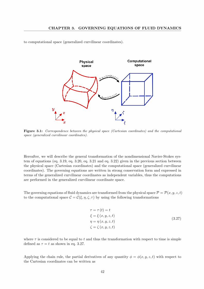
The Navier-Stokes system of equation (eq. 3.1, eq. 3.2, eq. 3.3 and eq. 3.4) are valid for anycoordinate system. We have previously expressed these equations in terms of a Cartesian co-ordinate system. For many applications it is more convenient to use a generalized curvilinearcoordinate system. The use of generalized curvilinear coordinates implies that a distorted regionin physical space is mapped into a rectangular region in the generalized curvilinear coordinatespace (figure 3.1). Often, the transformation is chosen so that the discretized equations aresolved in a uniform logically rectangular domain for 2D applications and an equivalent uniformlogically hexahedral domain for 3D applications. The transformation shall be such that there isa one-to-one correspondence of the grid points from the physical space (Cartesian coordinates)
41
CHAPTER 3. GOVERNING EQUATIONS OF FLUID DYNAMICS
to computational space (generalized curvilinear coordinates).
Figure 3.1: Correspondence between the physical space (Cartesian coordinates) and the computationalspace (generalized curvilinear coordinates).
Hereafter, we will describe the general transformation of the nondimensional Navier-Stokes sys-tem of equations (eq. 3.19, eq. 3.20, eq. 3.21 and eq. 3.22) given in the previous section betweenthe physical space (Cartesian coordinates) and the computational space (generalized curvilinearcoordinates). The governing equations are written in strong conservation form and expressed interms of the generalized curvilinear coordinates as independent variables, thus the computationsare performed in the generalized curvilinear coordinate space.
The governing equations of fluid dynamics are transformed from the physical space P = P(x, y, z, t)to the computational space C = C(%, &, ', #) by using the following transformations
# = # (t) = t
% = % (x, y, z, t)& = & (x, y, z, t)' = ' (x, y, z, t)
(3.27)
where # is considered to be equal to t and thus the transformation with respect to time is simpledefined as # = t as shown in eq. 3.27.
Applying the chain rule, the partial derivatives of any quantity ( = ((x, y, z, t) with respect tothe Cartesian coordinates can be written as
42

3.3. TRANSFORMATION OF THE GOVERNING EQUATIONS TOGENERALIZED CURVILINEAR COORDINATES
!(
!t=
!(
!#+ %t
!(
!%+ &t
!(
!&+ 't
!(
!'!(
!x= %x
!(
!%+ &x
!(
!&+ 'x
!(
!'!(
!y= %y
!(
!%+ &y
!(
!&+ 'y
!(
!'!(
!z= %z
!(
!%+ &z
!(
!&+ 'z
!(
!'
(3.28)
Then the governing equations may be transformed from physical space P to computational spaceC by replacing the Cartesian derivatives by the partial derivatives given in eq. 3.28, where theterms %x, &x, 'x, %y, &y, 'y, %z, &z, 'z, %t, &t and 't are called metrics (they represents the ratio of arclengths in the computational space C to that of the physical space P) and where %x representsthe partial derivative of % with respect to x, i.e. !%/!x, and so forth.
Figure 3.2: Transformation from physical space to computational space. Left: structured grid in physicalspace. Right: logically uniform grid in computational space.
In most cases, the transformation eq. 3.27 from physical space P to computational space C is notknown analytically, rather it is generated numerically by a grid generation scheme. That is, weusually are provided with just the x, y and z coordinates of the grid points and we numericallygenerate the metrics using finite di!erences. The metrics %x, &x, 'x, %y, &y, 'y, %z, &z, 'z, %t, &t and 't
appearing in eq. 3.28 can be determined in the following manner. First, we write down thedi!erential expressions of the inverse of the transformation eq. 3.27,
dt = t!d# + t"d% + t#d& + t$d'
dx = x!d# + x"d% + x#d& + x$d'
dy = y!d# + y"d% + y#d& + y$d'
dz = z!d# + z"d% + z#d& + z$d'
(3.29)
where the inverse of the transformation eq. 3.27 is
43

CHAPTER 3. GOVERNING EQUATIONS OF FLUID DYNAMICS
t = t (#) = #
x = x (%, &, ', #)y = y (%, &, ', #)z = z (%, &, ', #)
(3.30)
and recalling that for a grid that is not changing (moving, adapting or deforming)
!t
!#= 1 and
!t
!%=
!t
!&=
!t
!'= 0 thus
dt = d#
Expressing eq. 3.29 in matrix form, we obtain
!
""#
dtdxdydz
$
%%& =
!
""#
1 0 0 0x! x" x# x$
y! y" y# y$
z! z" z# z$
$
%%&
!
""#
d#d%d&d'
$
%%& (3.31)
In a like manner, we proceed with the transformation eq. 3.27, and we obtain the followingdi!erential expressions
d# = dt
d% = %tdt + %xdx + %ydy + %zdz
d& = &tdt + &xdx + &ydy + &zdz
d' = 'tdt + 'xdx + 'ydy + 'zdz
(3.32)
which can be written in matrix form as
!
""#
d#d%d&d'
$
%%& =
!
""#
1 0 0 0%t %x %y %z
&t &x &y &z
't 'x 'y 'z
$
%%&
!
""#
dtdxdydz
$
%%& (3.33)
By relating the di!erential expressions eq. 3.33 of the transformation eq. 3.27 to the di!erentialexpressions eq. 3.31 of the transformation eq. 3.30, so that the metrics
%x, &x, 'x, %y, &y, 'y, %z, &z, 'z, %t, &t, 't
can be found, we conclude that
!
""#
1 0 0 0%t %x %y %z
&t &x &y &z
't 'x 'y 'z
$
%%& =
!
""#
1 0 0 0x! x" x# x$
y! y" y# y$
z! z" z# z$
$
%%&
!1
(3.34)
44

3.3. TRANSFORMATION OF THE GOVERNING EQUATIONS TOGENERALIZED CURVILINEAR COORDINATES
This yields the following metrics relationships
%x = Jx (y#z$ " y$z#)%y = Jx (x$z# " x#z$)%z = Jx (x#y$ " x$y#)%t = " (#tx!%x + #ty!%y + #tz!%z)&x = Jx (y$z" " y"z$)&y = Jx (x"z$ " x$z")&z = Jx (x$y" " x"y$)&t = " (#tx!&x + #ty!&y + #tz!&z)'x = Jx (y"z# " y#z")'y = Jx (x#z" " x"z#)'z = Jx (x"y# " x#y")'t = " (#tx!'x + #ty!'y + #tz!'z)
(3.35)
For %t, &t and 't the following values are obtained after some manipulation
%t = Jx [x! (y$z# " y#z$) + y! (x#z$ " x$z#) + z! (x$y# " x#y$)]&t = Jx [x! (y"z$ " y$z") + y! (x$z" " x"z$) + z! (x"y$ " x$y")]'t = Jx [x! (y#z" " y"z#) + y! (x"z# " x#z") + z! (x#y" " x"y#)]
(3.36)
In eq. 3.35 and eq. 3.36, Jx is the determinant of the Jacobian matrix of the transformationdefined by
Jx =////! (%, &, ')! (x, y, z)
////
or
Jx =1
x" (y#z$ " y$z#)" x# (y"z$ " y$z") + x$ (y"z# " y#z")(3.37)
which can be interpreted as the ratio of the areas (volumes in 3D) in the computational space Cto that of the physical space P.
Once relations for the metrics and for the Jacobian of the transformation are determined, thegoverning equations eq. 3.19 are then written in strong conservation form as
!Q!t
+!Ei
!%+
!Fi
!&+
!Gi
!'=
!Ev
!%+
!Fv
!&+
!Gv
!'(3.38)
where
45

CHAPTER 3. GOVERNING EQUATIONS OF FLUID DYNAMICS
Q =QJx
Ei =1Jx
(%tQ + %xEi + %yFi + %zGi)
Fi =1Jx
(&tQ + &xEi + &yFi + &zGi)
Gi =1Jx
('tQ + 'xEi + 'yFi + 'zGi)
Ev =1Jx
(%xEv + %yFv + %zGv)
Ev =1Jx
(&xEv + &yFv + &zGv)
Ev =1Jx
('xEv + 'yFv + 'zGv)
(3.39)
The viscous stresses given by eq. 3.24 in the transformed computational space are
#xx =23
µ
ReL[2 (%xu" + &xu# + 'xu$)" (%yv" + &yv# + 'yv$) . . .
. . ." (%zw" + &zw# + 'zw$)]
#yy =23
µ
ReL[2 (%yv" + &yv# + 'yv$)" (%xu" + &xu# + 'xu$) . . .
. . ." (%zw" + &zw# + 'zw$)]
#zz =23
µ
ReL[2 (%zw" + &zw# + 'zw$)" (%xu" + &xu# + 'xu$) . . .
. . ." (%yv" + &yv# + 'yv$)](3.40)
#xy = #yx =µ
ReL(%yu" + &yu# + 'yu$ + %xv" + &xv# + 'xv$)
#xz = #zx =µ
ReL(%zu" + &zu# + 'zu$ + %xw" + &xw# + 'xw$)
#yz = #zy =µ
ReL(%zv" + &zv# + 'zv$ + %yw" + &yw# + 'yw$)
and the heat flux components given by eq. 3.23 in the computational space are
qx = " µ
($ " 1) M2#ReLPr
(%xT" + &xT# + 'xT$)
qy = " µ
($ " 1) M2#ReLPr
(%yT" + &yT# + 'yT$)
qz = " µ
($ " 1) M2#ReLPr
(%zT" + &zT# + 'zT$)
(3.41)
Equations eq. 3.38 and eq. 3.39 are the generic form of the governing equations written in strongconservation form in the transformed computational space C (see [14], [85] and [181] for a detailedderivation). The coordinate transformation presented in this section, follows the same develop-ment proposed by Viviand [202] and Vinokur [201], where they show that the governing equations
46

3.4. SIMPLIFICATION OF THE NAVIER-STOKES SYSTEM OF EQUATIONS:INCOMPRESSIBLE VISCOUS FLOW CASE
of fluid dynamics can be put back into strong conservation form after a coordinate transformationhas been applied.
Comparing the original governing equations eq. 3.19, eq. 3.20, eq. 3.21 and eq. 3.22 and the trans-formed equations eq. 3.38 and eq. 3.39, it is obvious that the transformed equations are morecomplicated than the original equations. Thus, a trade-o! is introduced whereby advantagesgained by using the generalized curvilinear coordinates are somehow counterbalanced by the re-sultant complexity of the equations. However, the advantages (such as the capability of usingstandard finite di!erences schemes and solving the equations in a uniform rectangular logicallygrid) by far outweigh the complexity of the transformed governing equations.
One final word of caution. The strong conservation form of the governing equations in thetransformed computational space C is a convenient form for applying finite di!erence schemes.However, when using this form of the equations, extreme care must be exercised if the grid ischanging (that is moving, adapting or deforming). In this case, a constraint on the way themetrics are di!erenced, called the geometric conservation law or GCL (see [50], [55] and [185]),must be satisfied in order to prevent additional errors from being introduced into the solution.
3.4 Simplification of the Navier-Stokes System of Equations: In-compressible Viscous Flow Case
Equations eq. 3.1, eq. 3.2, eq. 3.3 and eq. 3.4 with an appropriate equation of state and boundaryand initial conditions, governs the unsteady three-dimensional motion of a viscous Newtonian,compressible fluid. In many applications the fluid density may be assumed to be constant. Thisis true not only for liquids, whose compressibility may be neglected, but also for gases if theMach number is below 0.3 [6, 53]; such flows are said to be incompressible. If the flow is alsoisothermal, the viscosity is also constant. In this case, the dimensional governing equations inprimitive variable formulation (u, v, w, p) and written in compact conservative di!erential formreduce to the following set
! · (u) = 0!u!t
+! · (uu) ="!p
"+ )!2u
where ) is the kinematic viscosity and is equal ) = µ/". The same set of equations in nondimen-sional form is written as follows
! · (u) = 0!u!t
+! · (uu) = "!p +1
ReL!2u
which can be also written in nonconservative form (or advective/convective form [60])
! · u = 0!u!t
+ u ·!u = "!p +1
ReL!2u
or in expanded three-dimensional Cartesian coordinates
47

CHAPTER 3. GOVERNING EQUATIONS OF FLUID DYNAMICS
!u
!x+
!v
!y+
!w
!z= 0
!u
!t+ u
!u
!x+ v
!u
!y+ w
!u
!z= "!p
!x+
1ReL
'!2u
!x2+
!2u
!y2+
!2u
!z2
(
!v
!t+ u
!v
!x+ v
!v
!y+ w
!v
!z= "!p
!x+
1ReL
'!2v
!x2+
!2v
!y2+
!2v
!z2
(
!w
!t+ u
!w
!x+ v
!w
!y+ w
!w
!z= "!p
!x+
1ReL
'!2w
!x2+
!2w
!y2+
!2w
!z2
(
(3.42)
This form (the advective/convective form), provides the simplest form for discretization and iswidely used when implementing numerical methods for solving the incompressible Navier-Stokesequations, as noted by Gresho [60].
Equation eq. 3.42 governs the unsteady three-dimensional motion of a viscous, incompressibleand isothermal flow. This simplification is generally not of a great value, as the equations arehardly any simpler to solve. However, the computing e!ort may be much smaller than for thefull equations (due to the reduction of the unknowns and the fact that the energy equation isdecoupled from the system of equation), which is a justification for such a simplification. The setof equations eq. 3.42 can be rewritten in vector form as follow
!Q!t
+!Ei
!x+
!Fi
!y+
!Gi
!z=
!Ev
!x+
!Fv
!y+
!Gv
!z(3.43)
where Q is the vector containing the primitive variables and is given by
Q =
!
""#
0uvw
$
%%& (3.44)
and Ei, Fi and Gi are the vectors containing the inviscid fluxes in the x, y and z directions andare given by
Ei =
!
""#
uu2 + p
uvuw
$
%%& , Fi =
!
""#
vvu
v2 + pvw
$
%%& , Gi =
!
""#
wwuwv
w2 + p
$
%%& (3.45)
The viscous fluxes in the x, y and z directions, Ev, Fv and Gv respectively, are defined as follows
Ev =
!
""#
0#xx
#xy
#xz
$
%%& , Fv =
!
""#
0#yx
#yy
#yz
$
%%& , Gv =
!
""#
0#zx
#zy
#zz
$
%%& (3.46)
Since we made the assumptions of an incompressible flow, appropriate nondimensional terms and
48
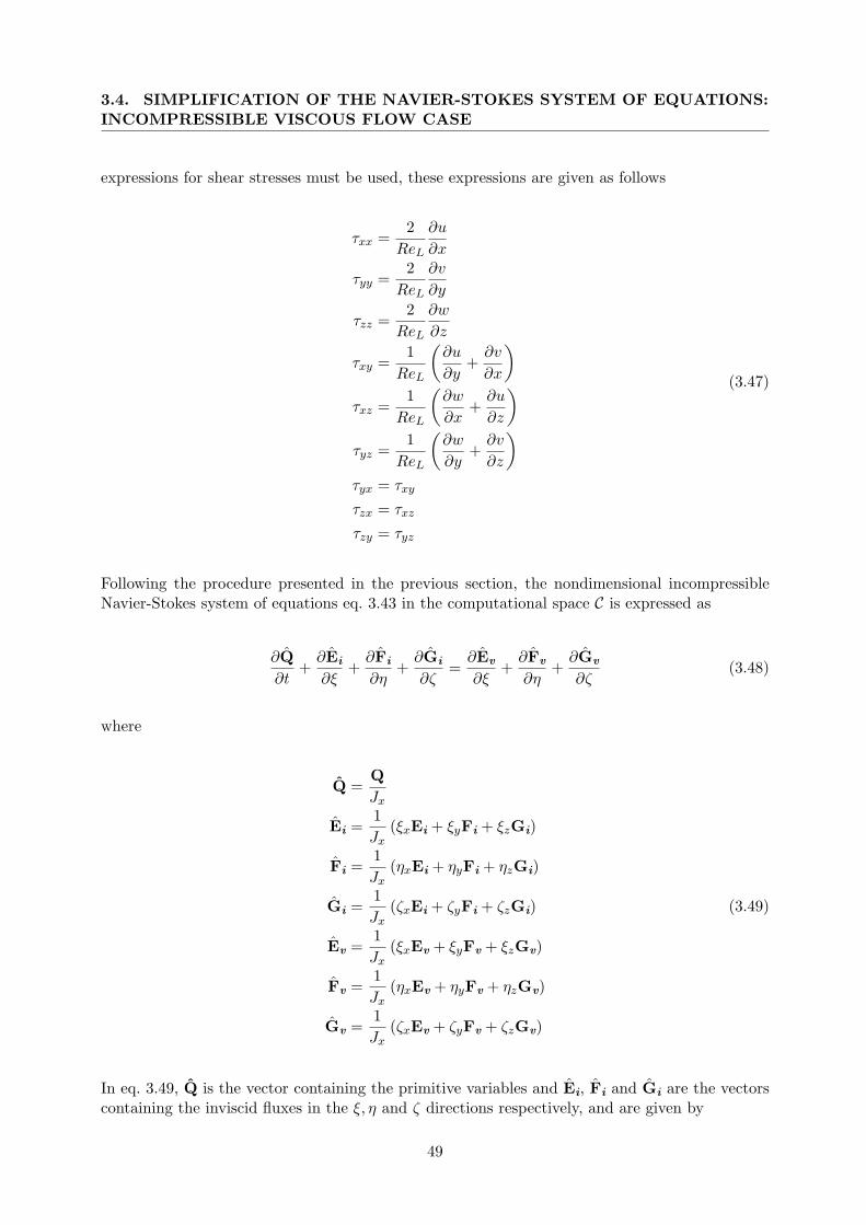
3.4. SIMPLIFICATION OF THE NAVIER-STOKES SYSTEM OF EQUATIONS:INCOMPRESSIBLE VISCOUS FLOW CASE
expressions for shear stresses must be used, these expressions are given as follows
#xx =2
ReL
!u
!x
#yy =2
ReL
!v
!y
#zz =2
ReL
!w
!z
#xy =1
ReL
'!u
!y+
!v
!x
(
#xz =1
ReL
'!w
!x+
!u
!z
(
#yz =1
ReL
'!w
!y+
!v
!z
(
#yx = #xy
#zx = #xz
#zy = #yz
(3.47)
Following the procedure presented in the previous section, the nondimensional incompressibleNavier-Stokes system of equations eq. 3.43 in the computational space C is expressed as
!Q!t
+!Ei
!%+
!Fi
!&+
!Gi
!'=
!Ev
!%+
!Fv
!&+
!Gv
!'(3.48)
where
Q =QJx
Ei =1Jx
(%xEi + %yFi + %zGi)
Fi =1Jx
(&xEi + &yFi + &zGi)
Gi =1Jx
('xEi + 'yFi + 'zGi)
Ev =1Jx
(%xEv + %yFv + %zGv)
Fv =1Jx
(&xEv + &yFv + &zGv)
Gv =1Jx
('xEv + 'yFv + 'zGv)
(3.49)
In eq. 3.49, Q is the vector containing the primitive variables and Ei, Fi and Gi are the vectorscontaining the inviscid fluxes in the %, & and ' directions respectively, and are given by
49
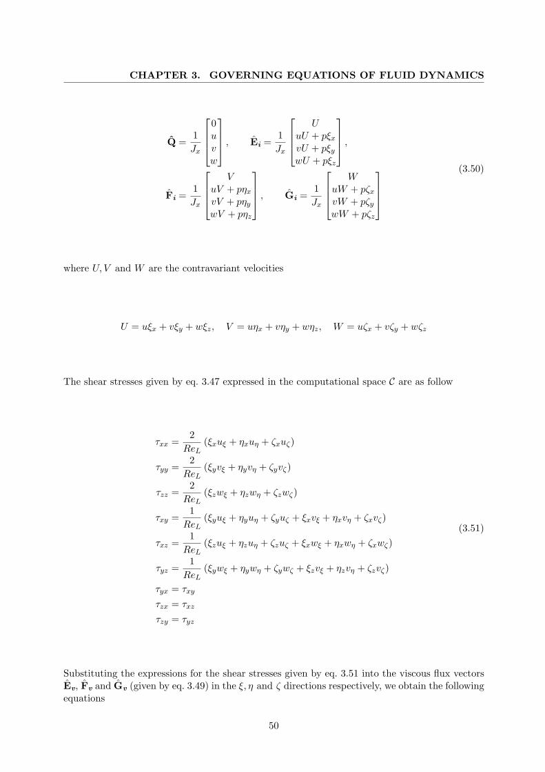
CHAPTER 3. GOVERNING EQUATIONS OF FLUID DYNAMICS
Q =1Jx
!
""#
0uvw
$
%%& , Ei =1Jx
!
""#
UuU + p%x
vU + p%y
wU + p%z
$
%%& ,
Fi =1Jx
!
""#
VuV + p&x
vV + p&y
wV + p&z
$
%%& , Gi =1Jx
!
""#
WuW + p'x
vW + p'y
wW + p'z
$
%%&
(3.50)
where U, V and W are the contravariant velocities
U = u%x + v%y + w%z, V = u&x + v&y + w&z, W = u'x + v'y + w'z
The shear stresses given by eq. 3.47 expressed in the computational space C are as follow
#xx =2
ReL(%xu" + &xu# + 'xu$)
#yy =2
ReL(%yv" + &yv# + 'yv$)
#zz =2
ReL(%zw" + &zw# + 'zw$)
#xy =1
ReL(%yu" + &yu# + 'yu$ + %xv" + &xv# + 'xv$)
#xz =1
ReL(%zu" + &zu# + 'zu$ + %xw" + &xw# + 'xw$)
#yz =1
ReL(%yw" + &yw# + 'yw$ + %zv" + &zv# + 'zv$)
#yx = #xy
#zx = #xz
#zy = #yz
(3.51)
Substituting the expressions for the shear stresses given by eq. 3.51 into the viscous flux vectorsEv, Fv and Gv (given by eq. 3.49) in the %, & and ' directions respectively, we obtain the followingequations
50

3.4. SIMPLIFICATION OF THE NAVIER-STOKES SYSTEM OF EQUATIONS:INCOMPRESSIBLE VISCOUS FLOW CASE
Ev =1
JxReL
!
""#
0a1u" + b1u# " c1v# + c2w# + b2u$ " d1v$ + d2w$
a1v" + c1u# + b1v# " c3w# + d1u$ + b2v$ " d3w$
a1w" " c2u# + c3v# + b1w# " d2u$ + d3v$ + b2w$
$
%%&
Fv =1
JxReL
!
""#
0a2u# + b1u" + c1v" " c2w" + b2u$ " e1v$ + e2w$
a2v# " c1u" + b1v" + c3w" + e1u$ + b3v$ " e3w$
a2w# + c2u" " c3v" + b1w" " e2u$ + e3v$ + b3w$
$
%%&
Gv =1
JxReL
!
""#
0a3u$ + b2u" + d1v" " d2w" + b3u# + e1v# " e2w#
a3v$ " c4u" + b2v" + d3w" " e1u# + b3v# + e3w#
a3w$ + d2u" " d3v" + b2w" + c8u# " e3v# + b3w#
$
%%&
(3.52)
where
a1 = %2x + %2
y + %2z , a2 = &2
x + &2y + &2
z , a3 = '2x + '2
y + '2z ,
b1 = %x&x + %y&y + %z&z, b2 = %x'x + %y'y + %z'z,
b3 = 'x&x + 'y&y + 'z&z,
c1 = %x&y " &x%y, c2 = &x%z " %x&z, c3 = %y&z " &y%z,
d1 = %x'y " 'x%y, d2 = 'x%z " %x'z, d3 = %y'z " 'y%z,
e1 = &x'y " 'x&y, e2 = 'x&z " &x'z, e3 = &y'z " 'y&z
(3.53)
equations eq. 3.52 and eq. 3.53 written in a more compact way, can be expressed as
Ev =1
JxReL
!
""#
0(!% ·!%)u" + (!% ·!&) u# + (!% ·!')u$
(!% ·!%) v" + (!% ·!&) v# + (!% ·!') v$
(!% ·!%) w" + (!% ·!&) w# + (!% ·!') w$
$
%%&
Fv =1
JxReL
!
""#
0(!& ·!%) u" + (!& ·!&)u# + (!& ·!') u$
(!& ·!%) v" + (!& ·!&) v# + (!& ·!') v$
(!& ·!%) w" + (!& ·!&) w# + (!& ·!') w$
$
%%&
Gv =1
JxReL
!
""#
0(!' ·!%)u" + (!' ·!&) u# + (!' ·!')u$
(!' ·!%) v" + (!' ·!&) v# + (!' ·!') v$
(!' ·!%) w" + (!' ·!&)w# + (!' ·!') w$
$
%%&
(3.54)
Equation eq. 3.48, together with eq. 3.49, eq. 3.50 and eq. 3.54, are the governing equations of anincompressible viscous flow written in strong conservation form in the transformed computationalspace C. Hence, we look for an approximate solution of this set of equations in a given domainD with prescribed boundary conditions !D and given initial conditions DU. So far, we have justpresented the governing equations; in the following chapters the grid generation method as wellas the numerical scheme for solving the governing equations will be explained.
51