Embed Size (px)
Citation preview

Tensor Programs: The Feynman Diagrams of Deep Learning
Greg Yang
MSR AI

Outline

Correlation Functions in Physics & ML

Correlation Functions in Physics
• Given a distribution on functions 𝜙:ℝ𝑘 → ℝ, the 2-point correlation function is defined to be𝐶2 𝑥1, 𝑥2 = 𝔼𝜙𝜙 𝑥1 𝜙 𝑥2
• Measure of order in a physical system (statmech)
• Measures “amplitude” of a particle going from x to y (QFT)
• Often calculated with Feynman Diagrams
Sou
rce: http
s://en.w
ikiped
ia.org/w
iki/Co
rrelation
_fun
ction
_(statistical_mech
anics)

Correlation Functions in ML
• Given a neural network, the last layer before the output is called the “embedding”• For an input 𝑥, write its embedding as Φ 𝑥 ∈ ℝ𝑚
• Consider the “2-point function”
𝐶2 𝑥1, 𝑥2 =1
𝑚
𝛼=1
𝑚
Φ 𝑥1 𝛼Φ 𝑥2 𝛼
• The 2-point function holds semantical information• The more semantically similar two inputs
are to each other, the larger the correlation of the embeddings
Credit:https://towardsdatascience.com/understanding-feature-engineering-part-4-deep-learning-methods-for-text-data-96c44370bbfa

Word2vec example
• Woman – queen = man – king
• Cats – cat = dogs – dog
• France – Paris = England - London
Credit: https://samyzaf.com/ML/nlp/word2vec2.png
More frequent words also usually have larger norms

Thus correlation functions are quite important in ML as well (though they don’t go by that name).

Some Physics of Neural Networks via Correlation Functions

Neural Network Terminologies
• Width = #neurons in a hidden layer
• Depth = #layers
https://medium.com/datadriveninvestor/when-not-to-use-neural-networks-89fb50622429
Depth
Wid
th

Wide Neural Networks
• Why do we care?
• The wider the better!• In fact this contradicts
classical learning theory orthodoxy
• So what happens at the infinite width limit?
Tan & Le 2019
𝑤 = width multiplier
???

Neural Networks at the Infinite-Width Limit

Gaussian Process Behavior
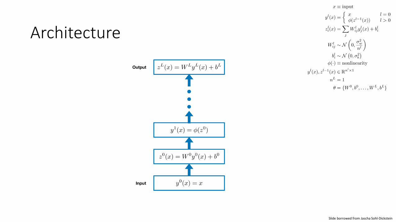
Architecture
Slide borrowed from Jascha Sohl-Dickstein

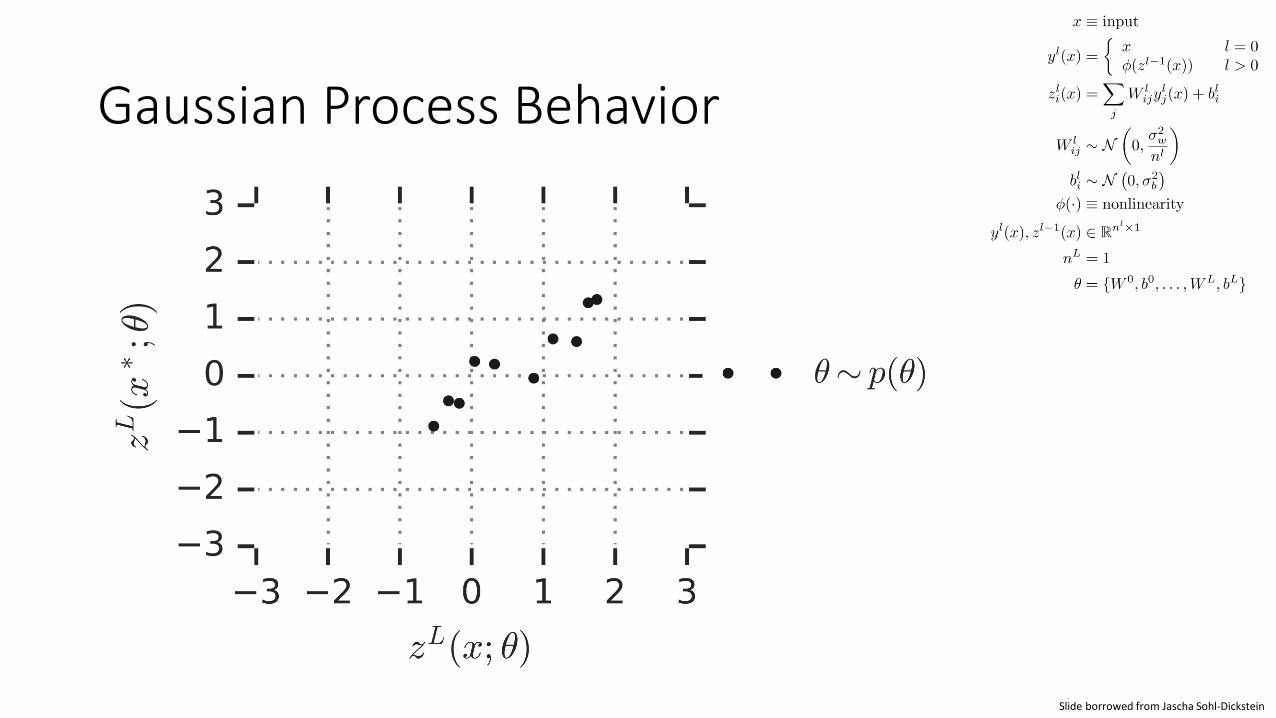
Gaussian Process Behavior
Slide borrowed from Jascha Sohl-Dickstein
Gaussian Process Behavior
Slide borrowed from Jascha Sohl-Dickstein

Gaussian Process Behavior
Slide borrowed from Jascha Sohl-Dickstein

Gaussian Process Behavior
Slide borrowed from Jascha Sohl-Dickstein

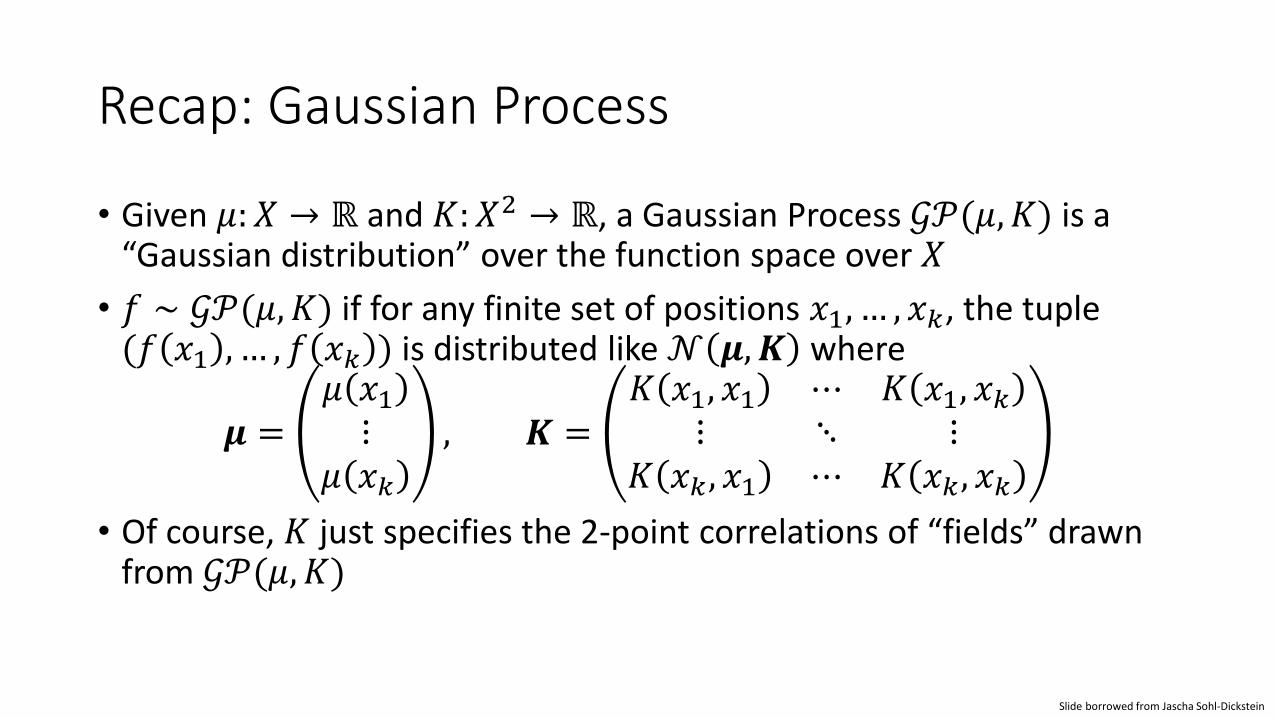
Recap: Gaussian Process
• Given 𝜇: 𝑋 → ℝ and 𝐾:𝑋2 → ℝ, a Gaussian Process 𝒢𝒫(𝜇, 𝐾) is a “Gaussian distribution” over the function space over 𝑋
• 𝑓 ∼ 𝒢𝒫(𝜇, 𝐾) if for any finite set of positions 𝑥1, … , 𝑥𝑘, the tuple (𝑓 𝑥1 , … , 𝑓 𝑥𝑘 ) is distributed like 𝒩 𝝁,𝑲 where
𝝁 =𝜇 𝑥1⋮
𝜇 𝑥𝑘
, 𝑲 =𝐾 𝑥1, 𝑥1 ⋯ 𝐾 𝑥1, 𝑥𝑘
⋮ ⋱ ⋮𝐾 𝑥𝑘 , 𝑥1 ⋯ 𝐾 𝑥𝑘 , 𝑥𝑘
Slide borrowed from Jascha Sohl-Dickstein
Recap: Gaussian Process
• Given 𝜇: 𝑋 → ℝ and 𝐾:𝑋2 → ℝ, a Gaussian Process 𝒢𝒫(𝜇, 𝐾) is a “Gaussian distribution” over the function space over 𝑋
• 𝑓 ∼ 𝒢𝒫(𝜇, 𝐾) if for any finite set of positions 𝑥1, … , 𝑥𝑘, the tuple (𝑓 𝑥1 , … , 𝑓 𝑥𝑘 ) is distributed like 𝒩 𝝁,𝑲 where
𝝁 =𝜇 𝑥1⋮
𝜇 𝑥𝑘
, 𝑲 =𝐾 𝑥1, 𝑥1 ⋯ 𝐾 𝑥1, 𝑥𝑘
⋮ ⋱ ⋮𝐾 𝑥𝑘 , 𝑥1 ⋯ 𝐾 𝑥𝑘 , 𝑥𝑘
• Of course, 𝐾 just specifies the 2-point correlations of “fields” drawn from 𝒢𝒫(𝜇, 𝐾)
Slide borrowed from Jascha Sohl-Dickstein

Universality of Gaussian Process Behavior
• For any neural network architecture, feedforward or recurrent, the network, when randomly initialized, becomes a Gaussian Process as its widths tend to ∞.
• Intuition: GP kernel = 2-point function of the last layer embeddingSimple RNN GRU Transformer Batchnorm
Yang 2019
What Happens when Depth →∞?

Architecture
Slide borrowed from Jascha Sohl-Dickstein
Schoenholz et al. 2017
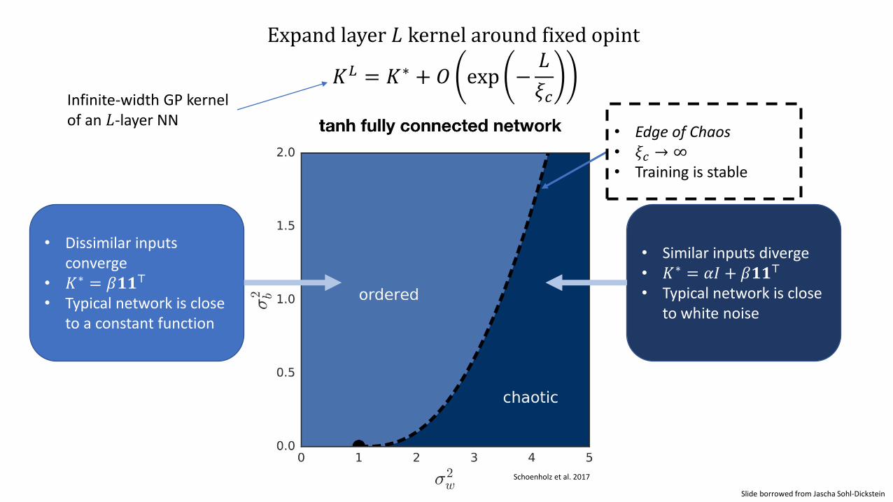
Expand layer 𝐿 kernel around fixed opint
𝐾𝐿 = 𝐾∗ + 𝑂 exp −𝐿
𝜉𝑐
• Dissimilar inputs converge
• 𝐾∗ = 𝛽𝟏𝟏⊤
• Typical network is close to a constant function
• Similar inputs diverge• 𝐾∗ = 𝛼𝐼 + 𝛽𝟏𝟏⊤
• Typical network is close to white noise
• Edge of Chaos• 𝜉𝑐 → ∞• Training is stable
Slide borrowed from Jascha Sohl-Dickstein
Infinite-width GP kernelof an 𝐿-layer NN

Using Edge of Chaos for Profit!!!
Slide borrowed from Jascha Sohl-Dickstein
!!!

Small Learning Rate Training
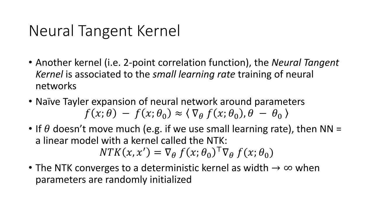
Neural Tangent Kernel
• Another kernel (i.e. 2-point correlation function), the Neural Tangent Kernel is associated to the small learning rate training of neural networks
• Naïve Tayler expansion of neural network around parameters𝑓 𝑥; 𝜃 − 𝑓 𝑥; 𝜃0 ≈ ∇𝜃 𝑓 𝑥; 𝜃0 , 𝜃 − 𝜃0
• If 𝜃 doesn’t move much (e.g. if we use small learning rate), then NN = a linear model with a kernel called the NTK:
𝑁𝑇𝐾 𝑥, 𝑥′ = ∇𝜃 𝑓 𝑥; 𝜃0⊤∇𝜃 𝑓(𝑥; 𝜃0)
• The NTK converges to a deterministic kernel as width → ∞ when parameters are randomly initialized

Universality of Neural Tangent Behavior
• For any neural network architecture, feedforward or recurrent, the NTK of the network converges deterministically, when the network is randomly initialized, as the network widths tend to ∞.
• If trained under small learning rate, then the network evolves like a linear model with the NTK kernel.
• These kernels have now achieved state-of-the-art in classification tasks with little data

How to Compute the Correlation Functions in a Wide Neural Net?

• The kernel of the limiting Gaussian process of an NN is essentially the 2-point function of its last layer embeddings Φ 𝑥 when the width 𝑛is large:
𝐾 𝑥, 𝑥′ ≈1
𝑛
𝑖=1
𝑛
Φ 𝑥 Φ 𝑥′ ≡ ⟨Φ 𝑥 Φ 𝑥′ ⟩
• In our example NN with 𝐿 layers, Φ 𝑥 = 𝑦𝐿(𝑥)
• So suffices to compute the 𝑛 → ∞ limit of ⟨𝑦𝑖𝐿 𝑥 𝑦𝑖
𝐿 𝑥′ ⟩

Feynman Diagrams?
• In the spirit of Feynman diagrams, we shall• Taylor expand all nonlinearities
• Say 𝜙 𝑥 = 𝑎0 + 𝑎1𝑥 + 𝑎2𝑥2 +⋯
• Algebra• Apply Wick’s theorem
• Let 𝑥 and 𝑥′ be two inputs𝑦𝑖𝐿 𝑥 𝑦𝑖
𝐿(𝑥′)
= ⟨𝑎02 + 𝑎0𝑎1𝑧𝑖
𝐿−1 𝑥 + 𝑎0𝑎1𝑧𝑖𝐿−1(𝑥′) + 𝑎1
2𝑧𝑖𝐿−1(𝑥)𝑧𝑖
𝐿−1(𝑥′) + ⋯ ⟩
= ⟨𝑎02+𝑎0𝑎1𝑊𝑖𝑗
𝐿−1𝑦𝑗𝐿−1(𝑥) + 𝑎0𝑎1𝑊𝑖𝑗
𝐿−1𝑦𝑗𝐿−1(𝑥′) + 𝑎1
2𝑊𝑖𝑗𝐿−1𝑦𝑗
𝐿−1(𝑥)𝑊𝑖′𝑗′
𝐿−1𝑦𝑗′𝐿−1(𝑥′) + ⋯ ⟩
= ⋯𝑔𝑒𝑡𝑠 𝑐𝑜𝑚𝑝𝑙𝑖𝑐𝑎𝑡𝑒𝑑⋯
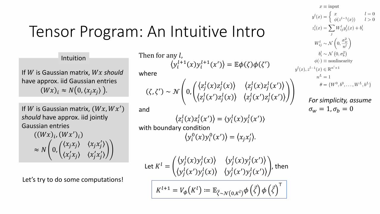
Tensor Program: An Intuitive Intro
If 𝑊 is Gaussian matrix, 𝑊𝑥 shouldhave approx. iid Gaussian entries
𝑊𝑥 𝑖 ≈ 𝑁 0, ⟨𝑥𝑗𝑥𝑗⟩ .
Intuition
If 𝑊 is Gaussian matrix, (𝑊𝑥,𝑊𝑥′)should have approx. iid jointly Gaussian entries
( 𝑊𝑥 𝑖 , 𝑊𝑥′ 𝑖)
≈ 𝑁 0,⟨𝑥𝑗𝑥𝑗⟩ ⟨𝑥𝑗𝑥𝑗
′⟩
⟨𝑥𝑗′𝑥𝑗⟩ ⟨𝑥𝑗
′𝑥𝑗′⟩
Then for any 𝑙,
𝑦𝑖𝑙+1 𝑥 𝑦𝑖
𝑙+1(𝑥′) = 𝔼𝜙 𝜁 𝜙 𝜁′
where
𝜁, 𝜁′ ∼ 𝒩 0,𝑧𝑗𝑙 𝑥 𝑧𝑗
𝑙 𝑥 𝑧𝑗𝑙 𝑥 𝑧𝑗
𝑙 𝑥′
𝑧𝑗𝑙 𝑥′ 𝑧𝑗
𝑙 𝑥 𝑧𝑗𝑙 𝑥′ 𝑧𝑗
𝑙 𝑥′
and
𝑧𝑖𝑙 𝑥 𝑧𝑖
𝑙 𝑥′ = ⟨𝑦𝑖𝑙 𝑥 𝑦𝑖
𝑙 𝑥′ ⟩with boundary condition
𝑦𝑖0 𝑥 𝑦𝑖
0 𝑥′ = 𝑥𝑗𝑥𝑗′ .
Let 𝐾𝑙 =𝑦𝑗𝑙 𝑥 𝑦𝑗
𝑙 𝑥 𝑦𝑗𝑙 𝑥 𝑦𝑗
𝑙 𝑥′
𝑦𝑗𝑙 𝑥′ 𝑦𝑗
𝑙 𝑥 𝑦𝑗𝑙 𝑥′ 𝑦𝑗
𝑙 𝑥′, then
For simplicity, assume𝜎𝑤 = 1, 𝜎𝑏 = 0
𝐾𝑙+1 = 𝑉𝜙 𝐾𝑙 ≔ 𝔼𝜁∼𝒩 0,𝐾𝑙 𝜙Ԧ𝜁 𝜙 Ԧ𝜁
⊤Let’s try to do some computations!

A sequence of vectors generated this way, along with the initial vectors and matrices, is known as a tensor program
Given some initial set of matrices and vectors, we can form new ones by:• (MatMul) Given a matrix 𝑊, and vector 𝑥, we can
generate 𝑊𝑥 or 𝑊⊤𝑥.
• (Nonlin) Given a bunch of vectors 𝑥1, … , 𝑥𝑘 of the same size, and a function 𝜙:ℝ𝑘 → ℝ, we can generate a new vector
𝜙(𝑥1, … , 𝑥𝑘)(with 𝜙 applied coordinatewise)
This motivates us to introduce a simple language for expressing computation for which the correlation function is easy to keep track of
Roughly Gaussian vectors, by our intuition:Think: preactivations
Roughly, image of Gaussian vectors.Think: activations
Think of these as the neural network parameters

𝐼𝑛𝑝𝑢𝑡:𝑊𝑖𝑗𝑙 ∼ 𝑁 0,
1
𝑛,
𝑤𝑖 , 𝑏𝑖𝑙 ∼ 𝑁(0, 1).
෪𝑥1 = 𝑊1𝑥 + 𝑏1
𝑥1 = 𝜙 ෪𝑥1
෪𝑥2 = 𝑊2𝑥1 + 𝑏2
𝑥2 = 𝜙 ෪𝑥2
⋮
𝑥𝐿 = 𝜙(෪𝑥𝐿)
𝑑෪𝑥𝐿 = 𝑤⊙𝜙′ ෪𝑥𝐿
𝑑𝑥𝐿−1 = 𝑊𝐿⊤𝑑෪𝑥𝐿
⋮
𝑑 ෪𝑥1 = 𝑑𝑥2 ⊙𝜙′ ෪𝑥1
𝑑𝑥 = 𝑊1⊤𝑑 ෪𝑥1
෪𝑥1′ = 𝑊1𝑥 + 𝑏1
𝑥1′ = 𝜙 ෪𝑥1′෪𝑥2′ = 𝑊2𝑥1′ + 𝑏2
𝑥2′ = 𝜙 ෪𝑥2′
⋮
𝑥𝐿′ = 𝜙(෪𝑥𝐿′)
𝑑 ෪𝑥𝐿′ = 𝑤 ⊙𝜙′ ෪𝑥𝐿′
𝑑𝑥𝐿−1′ = 𝑊𝐿⊤𝑑෪𝑥𝐿′⋮
𝑑 ෪𝑥1′ = 𝑑𝑥2′ ⊙ 𝜙′ ෪𝑥1′
𝑑𝑥′ = 𝑊1⊤𝑑 ෪𝑥1′
Think of 𝑤 as last layer gradient
Example Tensor Program: forward and backpropagation

Two Surprises of Tensor Programs

Surprise I:Universality of Tensor Program ExpressivityAlmost all modern architectures:Any composition of• Multilayer perceptron• Recurrent neural networks
• LSTM• GRUs
• Skip connection• Convolution• Pooling• Batch normalization• Layer normalization• Attention• etc
Both forward and backward propagation
Even SGD training!

Surprise II:Any tensor program has a “mean field theory” that allows us to calculate its correlation functions

𝑔1 𝑔2 𝑔3 𝑔𝑀
𝑛→∞
𝜓
𝜓
𝜓
𝜓
𝜓
𝜓
(
Average
1
𝑛
1
𝑛 (
(
(
(
(
)
)
)
)
)
)
𝔼𝑍 ~𝒩 𝜇,Σ
𝜓( )𝑎. 𝑠.
???
If - the initial set of vectors and matrices of a tensor program are all randomized as Gaussians, and- all the vectors in a tensor program are 𝑔1, … , 𝑔𝑀, then for any 𝜓:ℝ𝑀 → ℝ
Roughly speaking, each vector 𝑔𝑖 will be coordinatewise iid, but for each 𝛼, the coordinate-slice (𝑔𝛼
1 , … , 𝑔𝛼𝑀) has a nonseparable joint distribution which is some image of
𝒩 𝜇, Σ .
All of the correlation functions we mentioned can be computed by applying this theorem to an appropriate tensor program
For correlation, take 𝜓to be the product function.
𝜇 and Σ are some mean and covariance matrices that are computed recursively like in the example we did.
e.g. 𝑔2 = 𝑊 𝑔1
e.g. 𝑔3 = 𝜙 𝑔1, 𝑔2

Let 𝐾𝑙 =𝑦𝑗𝑙 𝑥 𝑦𝑗
𝑙 𝑥 𝑦𝑗𝑙 𝑥 𝑦𝑗
𝑙 𝑥′
𝑦𝑗𝑙 𝑥′ 𝑦𝑗
𝑙 𝑥 𝑦𝑗𝑙 𝑥′ 𝑦𝑗
𝑙 𝑥′, then
For simplicity, assume𝜎𝑤 = 1, 𝜎𝑏 = 0
𝐾𝑙+1 = 𝑉𝜙 𝐾𝑙 ≔ 𝔼𝜁∼𝒩 0,𝐾𝑙 𝜙Ԧ𝜁 𝜙 Ԧ𝜁
⊤
𝐾0 =𝑥𝑖𝑥𝑖 𝑥𝑖𝑥𝑖
′
𝑥𝑖′𝑥𝑖 𝑥𝑖
′𝑥𝑖′
and ∀𝑖, (𝑧𝑖𝑙 𝑥 , 𝑧𝑖
𝑙(𝑥′)) ≈ 𝒩(0, 𝐾𝑙)
𝑧0 𝑥
𝑛→∞
𝜓
𝜓
𝜓
𝜓
𝜓
𝜓
(
Average
1
𝑛
1
𝑛 (
(
(
(
(
)
)
)
)
)
)
𝔼𝑍0 ~𝒩 0,𝐾0
𝜓( )𝑎. 𝑠.
𝑧0 𝑥′
𝑍10 𝑍2
0
Example

Let 𝐾𝑙 =𝑦𝑗𝑙 𝑥 𝑦𝑗
𝑙 𝑥 𝑦𝑗𝑙 𝑥 𝑦𝑗
𝑙 𝑥′
𝑦𝑗𝑙 𝑥′ 𝑦𝑗
𝑙 𝑥 𝑦𝑗𝑙 𝑥′ 𝑦𝑗
𝑙 𝑥′, then
For simplicity, assume𝜎𝑤 = 1, 𝜎𝑏 = 0
𝐾𝑙+1 = 𝑉𝜙 𝐾𝑙 ≔ 𝔼𝜁∼𝒩 0,𝐾𝑙 𝜙Ԧ𝜁 𝜙 Ԧ𝜁
⊤
𝐾0 =𝑥𝑖𝑥𝑖 𝑥𝑖𝑥𝑖
′
𝑥𝑖′𝑥𝑖 𝑥𝑖
′𝑥𝑖′
and ∀𝑖, (𝑧𝑖𝑙 𝑥 , 𝑧𝑖
𝑙(𝑥′)) ≈ 𝒩(0, 𝐾𝑙)
𝑧0 𝑥
𝑛→∞
𝜓
𝜓
𝜓
𝜓
𝜓
𝜓
(
Average
1
𝑛
1
𝑛 (
(
(
(
(
)
)
)
)
)
)
𝔼𝑍0 ~𝒩 0,𝐾0 ,
𝑍1∼𝒩(0,𝑉𝜙 𝐾0 )
𝜓 ( )𝑎. 𝑠.
𝑧0 𝑥′
𝑍10 𝑍2
0
𝑧1 𝑥 𝑧1 𝑥′
𝑍11 𝑍2
1
Example

Let 𝐾𝑙 =𝑦𝑗𝑙 𝑥 𝑦𝑗
𝑙 𝑥 𝑦𝑗𝑙 𝑥 𝑦𝑗
𝑙 𝑥′
𝑦𝑗𝑙 𝑥′ 𝑦𝑗
𝑙 𝑥 𝑦𝑗𝑙 𝑥′ 𝑦𝑗
𝑙 𝑥′, then
For simplicity, assume𝜎𝑤 = 1, 𝜎𝑏 = 0
𝐾𝑙+1 = 𝑉𝜙 𝐾𝑙 ≔ 𝔼𝜁∼𝒩 0,𝐾𝑙 𝜙Ԧ𝜁 𝜙 Ԧ𝜁
⊤
𝐾0 =𝑥𝑖𝑥𝑖 𝑥𝑖𝑥𝑖
′
𝑥𝑖′𝑥𝑖 𝑥𝑖
′𝑥𝑖′
and ∀𝑖, (𝑧𝑖𝑙 𝑥 , 𝑧𝑖
𝑙(𝑥′)) ≈ 𝒩(0, 𝐾𝑙)
𝑧0 𝑥
𝑛→∞
𝜓
𝜓
𝜓
𝜓
𝜓
𝜓
(
Average
1
𝑛
1
𝑛 (
(
(
(
(
)
)
)
)
)
)
𝔼𝑍0 ~𝒩 0,𝐾0 ,
𝑍1∼𝒩(0,𝑉𝜙 𝐾0 ),
𝑍2∼𝒩(0,𝑉𝜙∘𝑉𝜙 𝐾0 )
𝜓 ( )𝑎. 𝑠.
𝑧0 𝑥′
𝑍10 𝑍2
0
𝑧1 𝑥 𝑧1 𝑥′
𝑍11 𝑍2
1
𝑧2 𝑥 𝑧2 𝑥′
𝑍12 𝑍2
2
Example

Tensor Programs Summary language technique
framework
A language for specifying computation graph involving matrices and vectors
Behavioral insight of the computation when the dimensions → ∞
Express deep neural network forward computation in a tensor program
Gaussian process behavior when the widths → ∞
language
technique
framework
e.g.

Consequences
• Universality of Gaussian Process behavior
• Universality of Neural Tangent Kernel behavior
• Phase transitions for different neural architectures
• New proofs of semicircle and Marchenko-Pastur laws
• Jacobian singular value of wide neural networks
• State Evolution for Approximate Message Passing algorithm in Compressed Sensing
• Gradient Independence phenomenon
• More in the paper!

Tensor Programs and Feynman Diagrams

Feynman Diagrams
• Perturbative (small 𝑔)
• Series Expansion
• Diagrams reflect particle interaction
• Handles interaction from higher order terms in the action
• Organizing principle for particle physics
Tensor Programs
• Infinite-Width Limit (large 𝑛)
• Recursive Computation
• Programs reflect neural network computation
• Handles interactions from coordinatewise nonlinearities
• I hope would become the organizing principle for the theory of deep learning
Differences and Similarities

Concrete Example in Random Matrix Theory
Feynman Diagrams
• Symmetric matrices 𝐴 with distribution
∝ exp −𝑡𝑟 𝐴2 − 𝑡𝑟 𝐴4
Tensor Programs
• Symmetric matrices 𝐴 with
𝐴𝑖𝑗 = 𝑊𝑖𝑗
𝑖′
𝑊𝑖′𝑗
𝑗
𝑊𝑖𝑗′
where 𝑊𝑖𝑗 is a symmetric Gaussian matrix (i.e. GOE)
• In general, can study jacobiansingular values of random deep neural networks

My Question to Physicists
• “Tensor Programs” seems like the “right” language for the theory of deep learning
• Some very shiny, attractive mathematics is now possible as a result
• Does it help perform calculations in physics?

Papers
https://arxiv.org/abs/1902.04760
Scaling Limits of Wide Neural Networks Wide NNs are GPs
https://arxiv.org/abs/1910.12478