Temporal video segmentation and classification of edit effects

Temporal video segmentation and classification of edit effects

Sarah Porter*, Majid Mirmehdi, Barry Thomas

Department of Computer Science, University of Bristol, Bristol BS8 1UB, UK

Accepted 13 August 2003

Abstract

The process of shot break detection is a fundamental component in automatic video indexing, editing and archiving. This paper introduces

a novel approach to the detection and classification of shot transitions in video sequences including cuts, fades and dissolves. It uses the

average inter-frame correlation coefficient and block-based motion estimation to track image blocks through the video sequence and to

distinguish changes caused by shot transitions from those caused by camera and object motion. We present a number of experiments in which

we achieve better results compared with two established techniques.

q 2003 Elsevier B.V. All rights reserved.

Keywords: Shot transitions; Shot break detection; Shot classification; Video segmentation

1. Introduction

Indexing and annotating large quantities of film and

video material is becoming an increasing problem through-

out the media industry, particularly where archived material

is concerned. Manually indexing video content is currently

the most accurate method but it is a very time consuming

process. Considerable amounts of archived data remain

unindexed which often leads to the production of new film

instead of the reutilisation of existing material. An efficient

video indexing technique is to temporally segment a

sequence into shots, where a shot is defined as a sequence

of frames captured from a single camera operation, and then

select representative key-frames to create an indexed

database. Hence, a small subset of frames can be used to

retrieve information from the video and enable content-

based video browsing.

There are two different types of transitions that can occur

between shots: abrupt (discontinuous) shot transitions also

referred to as cuts; or gradual (continuous) shot transitions

such as fades, dissolves and pushes or wipes. A cut is an

instantaneous change from one shot to another. During a

fade, a shot gradually appears from, or disappears to, a

constant image. A dissolve occurs when the first shot fades

out whilst the second shot fades in. There are hundreds of

different pushes or wipes, and all are considered to be

special transitional effects [1]. One example is when the new

shot pushes the last shot off the screen to the left, right, up or

down. In general during a wipe, the new shot is revealed by

a moving boundary in the form of a line or pattern.

Shots unified by a common locale or event are grouped

together into scenes. Although the cut is the simplest, most

common way of moving from one shot to the next, gradual

transitions are often used at scene boundaries to emphasis

the change in content of the sequence [2]. Hence, detecting

gradual transitions is particularly important for the identi-

fication of key-frames. The most common edit effects used

in video sequences are cuts, fades and dissolves [1]. In fact,

the data set used in this paper contains 450 cuts, 79 fade-ins,

74 fade-outs, 114 dissolves and only 5 wipes over a total of

21580 frames.

In the case of shot cuts, the content change is usually

large and easier to detect than the content change during a

gradual transition [3,4]. Fig. 1 shows a sequence of four

consecutive frames with a shot cut occurring between the

second and third frame. The significant inter-frame

difference during the shot cut is clearly shown. In contrast,

Fig. 2 shows six frames during a dissolve and illustrates that

the inter-frame difference during a gradual transition is

small. Indeed, the content change caused by camera

operations, such as pans, tilts or zooms and object move-

ment can be of the same magnitude as those caused by

gradual transitions. This makes it difficult to differentiate

0262-8856/$ - see front matter q 2003 Elsevier B.V. All rights reserved.

doi:10.1016/j.imavis.2003.08.014

Image and Vision Computing 21 (2003) 1097–1106

www.elsevier.com/locate/imavis

* Corresponding author.

E-mail address: [email protected] (S. Porter).

http://www.elsevier.com/locate/imavis

between changes caused by a continuous edit effect and

those caused by object and camera motion without also

incurring a large number of false positives. A comparison of

recent algorithms shows that the false positive rate when

detecting dissolves is usually unacceptably high, indicating

that reliable dissolve detection is still an unsolved problem

[3]. In this paper, we introduce a novel approach for the

detection and classification of the most commonly occurring

shot transitions: cuts, fades and dissolves.

Section 2 presents a brief overview of previous

approaches to video segmentation. In Section 3 we propose

a method designed explicitly to detect shot cuts using block-

based motion compensation. Normalised correlation

implemented in the frequency domain is used to estimate

the motion for each block. In Section 4, we extend the

algorithm for shot cut detection to detect fades and

dissolves. The proposed method uses block tracking to

differentiate between changes caused by gradual effects and

those caused by object and camera motion and it has been

designed to handle some of the shortcomings of previous

methods [5,6]. Experimental results confirming the validity

of the approach are presented and discussed in Section 5.

2. Previous work

Most of the existing methods for shot cut detection use

some inter-frame difference metric applied to various

features related to the visual content of a video. A frame

pair where this difference is greater than some predefined

threshold is considered to contain a shot cut. For each

selected feature, a number of suitable metrics can be

applied. In this section, we only outline the main

contributions but good summaries and comparisons of

features and metrics used for video segmentation with

respect to the quality of results obtained can be found in

Fig. 1. Four consecutive frames containing a shot cut between the second and third frame.

Fig. 2. Frames from a dissolve which occurs over 25 frames.

S. Porter et al. / Image and Vision Computing 21 (2003) 1097–11061098

several references [2–4,7–9]. Arguably, the simplest of

these methods is pair-wise pixel comparison, or frame

differencing. This compares the corresponding pixels

between two frames to determine how many have changed

[6]. The drawback of frame differencing is that it is sensitive

to small camera and object motions which can lead to a high

number of false positives [9]. Zhang et al. reduced the

effects of motion and noise by firstly applying a 3 £ 3

averaging filter [6]. They also suggested a more robust

method based on dividing a frame into regions and

comparing corresponding regions instead of individual

pixels. Regions were compared on the basis of second-

order statistical characteristics of their intensity values using

the likelihood ratio as the disparity metric [10]. This method

is less sensitive to local object motion but can still lead to

false positives in the presence of large object and camera

motions. A potential problem with the likelihood ratio is

that two regions may have the same mean and variance but

completely different probability functions. In such a case, a

shot cut would be missed.

Instead of comparing features based on individual pixels

or regions, features of the entire image have been used for

comparison to reduce further the sensitivity to object and

camera motion. For example, the average intensity measure

compares the average of the intensity values for each frame

pair [11]. Another global feature which has been used is a

histogram of intensity values [2,4,6,12]. An intensity

histogram of an image describes the distribution of the

intensities while ignoring the spatial distribution of pixels

within an image. The basic idea of using histograms is that

two frames with unchanging background and unchanging

objects will have similar intensity distributions even in the

presence of object and camera motion. A shot cut is detected

if the bin-wise difference between the histograms of two

consecutive frames exceeds some threshold. A disadvantage

of histogram-based (HB) methods is that a shot cut may be

missed between two shots with similar intensity distri-

butions but different content. To overcome this, Nagasaka

and Tanaka proposed dividing each frame into 16 blocks

and computing the difference between local histograms

[12]. They also removed the eight largest differences before

computing a single difference metric. This way, the method

is still robust to local motions within a region, and by

discarding the largest differences the method becomes less

sensitive to large object and camera motions. One drawback

is that this method may miss a cut between two shots with

similar backgrounds because the blocks that have changed

are the very ones being removed. They also compared

several different statistics on grey-level and colour histo-

grams and found the best performance was obtained by

using the x 2 test to compare colour histograms [13]. Each

pixel is represented by a colour code obtained by merging

the two most significant bits of each RGB component. This

also helped reduce the effect of changes in the luminance.

HB methods are the most common approach to shot cut

detection in use today, since they offer a good trade-off

between accuracy and computational efficiency [2,4,6,12].

All of the previously mentioned algorithms have been

devised for shot cut detection only. The difference between

a frame pair during a gradual transition is much smaller than

the difference that occurs during a shot cut. Lowering the

threshold to detect such small differences may result in

many false detections due to the differences caused by

camera and object motion. Zhang et al. proposed a twin

comparison technique comparing the histogram difference

with two thresholds [6]. A lower threshold was used to

detect small differences that occur for the duration of the

gradual transition while a higher threshold was used in the

detection of shot cuts and gradual transitions. This method

can fail when camera operations such as pans generate a

change in the colour distribution similar to that caused by a

gradual transition. To overcome this, they suggested

analysing the motion between frames to identify camera

operations such as pans, tilts and zooms. Where this type of

motion is identified the gradual transition is assumed to be

false to reduce the number of false positives. However, this

means that gradual transitions containing object or camera

motions will not be detected.

Motion-based algorithms (MB) have been proposed to

distinguish between changes caused by motion and those

caused by an edit effect [2,4,14]. Shahraray noted that

block-based comparison is usually performed by super-

imposing each block of the first image on exactly the same

location of the second image [6,12,14]. It was suggested that

a more robust measure can be obtained by motion

compensating blocks prior to calculating the block-wise

difference metrics. Shahraray used a weighted sum of the

motion-compensated pixel differences as the disparity

metric [14]. If this difference measure exceeds some

threshold a shot cut is detected. Gradual transitions are

detected by locating a sustained small increase in the

difference metric. Such methods may detect false positives

if there exists several blocks with poor matches as a result of

multiple motions within a block or in the presence of

motions that violate the translational model, while the

majority of blocks match well. To overcome the problem of

such outliers, Shahraray used an order statistic filter to

combine the disparity metrics of all the blocks [14]. In this

method, the values for each block are sorted in ascending

order and a weighted sum is computed where the

coefficients for each match value are assigned according

to the position of the value in the sorted list. While this may

reduce the chances of detecting shot transitions between

scenes with shared backgrounds, by choosing the coeffi-

cients properly it reduces the number of false detections in

the presence of several extremely bad matches compared to

the use of a linear combination of the similarity metrics.

Lupatini et al. also evaluate the motion compensated

difference values of each block [4]. They noted that since

the difference values are obtained by a pixel–pixel

comparison the method can still be highly sensitive to

S. Porter et al. / Image and Vision Computing 21 (2003) 1097–1106 1099

local motions. In order to overcome this problem, instead of

considering pixel differences, the average of the luminance

function was evaluated for each block. Instead of computing

a motion compensated disparity metric, Akutsu et al.

analysed the motion field measured between two frames

to detect shot cuts [15]. The disparity value between two

consecutive frames was then computed as the inverse of

motion smoothness.

Zabih et al. proposed another method to detect abrupt and

gradual transitions by checking the spatial distribution of

exiting and entering edge pixels [5]. Transitions were

identified by examining the relative values of the entering

and exiting edge percentages. To make the algorithm more

robust with respect to camera motions the two frames were

registered before comparison. However, despite the global

motion compensation this method is still sensitive to object

motion and camera motions such as zooms. Lienhart

proposed two algorithms, one to detect fades and the other

dissolves [3]. The first method detects fades by examining

the standard deviation of pixel intensities, which exhibits a

characteristic pattern during a fade. The second method is

based on the idea that there is a loss of contrast in an image

during a dissolve. The author described an edge-based

contrast feature, which emphasises the loss in contrast to

enable dissolve detection. One further approach for

detecting specifically dissolves is to monitor the temporal

quadratic behaviour of the variance of the pixel intensities

which was first proposed by Alattar, but has been modified

by other authors [16,17]. During a dissolve the intensity

variance starts to decrease at the beginning of a transition,

reaches its minimum in the middle and starts to increase

towards the end of the transition. Hence, the transition is

detected by locating this pattern in a series of variances.

However, a problem of this approach is that the pattern is

not sufficiently pronounced due to noise and motion in the

video [8].

The majority of the existing methods for detecting shot

transitions are weakened by camera and object motion and

sudden changes in the mean intensity within a shot. Yusoff

et al. proposed a method for shot cut detection which uses a

combination of multiple experts [18]. The experts them-

selves are stand-alone methods to detect shot cuts like those

mentioned above. However, they suggested that because

each method performs well in different circumstances,

significantly better results can be obtained by combining

these methods, as opposed to using each on their own.

Several authors have also proposed methods to detect the

type of motions that cause a sustained increase in the

disparity metric similar to that caused by a gradual transition

to reduce the number of false detections [6,14]. However, as

mentioned earlier these methods can then fail to detect

gradual transitions in the presence of such motion before,

during or after the transition. The conclusion must be that, a

shot transition detection method is still required that is

robust in the presence of camera and object motion and

changes in the global illumination.

3. Shot cut detection

We propose a MB to identify shot cuts which deals

inherently with object and camera motion. It uses block-

matching motion compensation to generate an inter-frame

difference metric. For each block in frame n; the best match

in a neighbourhood around the corresponding block in

frame n þ 1 is sought. This is achieved by calculating the

normalised correlation between blocks and locating the

maximum correlation coefficient. Calculating the normal-

ised correlation in the spatial domain is, however,

prohibitively expensive unless the blocks are small.

Hence, we perform normalised correlations in the frequency

domain [19] defined by:

rðjÞ ¼F21{x̂1ðvÞx̂

p2ðvÞ}ffiffiffiffiffiffiffiffiffiffiffiffiffiffiffiffiffiffiffiffiffiffiffiffiffiffiffiffiffiffiffiffiÐ

lx̂1ðvÞl2

dvÐlx̂2ðvÞ

2 dv

q ð1Þ

where j and v are the spatial and spatial frequency

coordinate vectors, respectively, x̂iðvÞ denotes the Fourier

transform of block xiðjÞ; F21 denotes the inverse Fourier

operator and p is the complex conjugate. A high-pass filter

is applied to each image before performing the correlations

to accentuate the contributions from higher spatial frequen-

cies, since a correlation field derived from high-pass regions

will contain more detectable peaks. Correlation fields

derived from low-pass regions will result in a flat correlation

field leading to inaccurate peak detection [20]. For this

reason, blocks with insufficient energy are not used. A

consequence of applying the high-pass filter is that the mean

of the image is removed. Hence, the correlation between

blocks is invariant to changes in the mean intensity. By

normalising the correlation, the method is insensitive to a

positive scaling of the image intensities. Most of the

previous methods for shot cut detection may falsely detect a

shot cut where sudden intensity changes occur within a shot,

for example, where there is a change in the lighting

conditions. By applying a high-pass filter and performing

normalised correlation our method is robust to changes in

the global illumination.

The location of the maximum correlation coefficient is

used to find the offset of each block in frame n þ 1 from its

position in frame n: Previous approaches use the estimated

motion vectors to calculate the motion-compensated frame

difference [14]. In contrast, our approach uses only the value

of the maximum correlation coefficient, as a goodness-of-fit

measure for each block. The value of the goodness-of-fit

measure lies between 0 and 1, where a value of 0 indicates a

complete mismatch and a value of 1 indicates a perfect

match. Fig. 3(a) shows the correlation field which resulted

from the correlation between two blocks from a frame pair

within the same shot and Fig. 3(b) shows the correlation

field from a frame pair containing a shot cut. Between two

frames belonging to the same shot, the goodness-of-fit for

the majority of the blocks should be close to 1.0, indicating


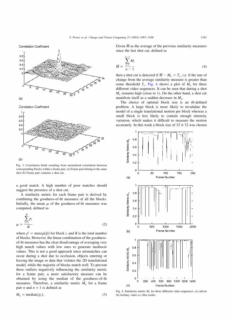
a good match. A high number of poor matches should

suggest the presence of a shot cut.

A similarity metric for each frame pair is derived by

combining the goodness-of-fit measures of all the blocks.

Initially, the mean m of the goodness-of-fit measures was

computed, defined as

m ¼

XB

i¼1

pi

Bð2Þ

where pi ¼ maxðrðjÞÞ for block i; and B is the total number

of blocks. However, the linear combination of the goodness-

of-fit measures has the clear disadvantage of averaging very

high match values with low ones to generate mediocre

values. This is not a good approach since mismatches can

occur during a shot due to occlusion, objects entering or

leaving the image or data that violates the 2D translational

model, while the majority of blocks match well. To prevent

these outliers negatively influencing the similarity metric

for a frame pair, a more satisfactory measure can be

obtained by using the median of the goodness-of-fit

measures. Therefore, a similarity metric Mn for a frame

pair n and n þ 1 is defined as

Mn ¼ median{pi}: ð3Þ

Given �M as the average of the previous similarity measures

since the last shot cut, defined as

�M ¼

Xn21

i¼1

Mi

n 2 1ð4Þ

then a shot cut is detected if �M 2 Mn . Tc; i.e. if the rate of

change from the average similarity measure is greater than

some threshold Tc: Fig. 4 shows a plot of Mn for three

different video sequences. It can be seen that during a shot

Mn remains high (close to 1). On the other hand, a shot cut

manifests itself as a sudden decrease in Mn:

The choice of optimal block size is an ill-defined

problem. A large block is more likely to invalidate the

model of a single translational motion per block whereas a

small block is less likely to contain enough intensity

variation, which makes it difficult to measure the motion

accurately. In this work a block size of 32 £ 32 was chosen

Fig. 3. Correlation fields resulting from normalised correlation between

corresponding blocks within a frame pair. (a) Frame pair belong to the same

shot (b) Frame pair contains a shot cut.

Fig. 4. Similarity metric Mn for three different video sequences. (a) advert

(b) holiday video (c) film trailer.


empirically as it gives an acceptable trade-off between

accuracy and the resolution of the motion field (using

images with typical dimensions 256 £ 256).

4. Detecting fades and dissolves

The method described above responds well to shot cuts.

In this section we describe the extension of this method to

also detect fades and dissolves. As in shot cut detection,

most of the previous approaches to detecting gradual

transitions are also sensitive to object and camera motions.

We propose a method that can differentiate between

changes caused by a gradual transition from those caused

by camera and object motion.

The shot cut detection method described in Section 3 can

be straightforwardly extended to detect fades. The end of a

fade-out and the start of a fade-in is marked by a constant

image. A constant image contains very little, if any, high-

pass energy. Therefore, correlation of an image with a

constant image results in Mn ¼ 0 which can be used to

identify the end of a fade-out and the start of a fade-in.

However, gradual transitions occur over a number of frames

so knowledge of the boundaries of the edit effect is required.

A fade is a scaling of the pixel intensities over time which

can be observed in the standard deviation of the pixel

intensities [3]. If Mn falls to 0 and the standard deviation of

the pixel intensities decreased prior to this, the frame where

the standard deviation started to decrease is marked as the

first frame of the fade-out. The decrease in the standard

deviation must have occurred over more than two frames to

distinguish fade-outs from a shot cut to a constant image.

Similarly, if the standard deviation of the pixel intensities

increases after the similarity metric increases from 0, the

frame where the standard deviation becomes constant is

marked as the end of the fade-in. Again, this must have

occurred over more than two frames. Initially, to compute

where the standard deviation becomes constant after a fade-

in, the standard deviation of frame n; denoted sn; was

compared to the standard deviation of frame n 2 1; sn21: If

sn # sn21 then the end of the fade-in was marked.

However, we observed that often the scaling factor is not

altered for every frame but only every other frame.

Therefore, the end of a fade-in would be marked too

early. Hence, the end of the fade-in was marked when

sn #sn21 þ sn22

2:

A similar comparison is used to detect the start of a fade-out.

Extending this method to detect dissolves is somewhat

more involved. The difference between each frame pair

during a dissolve is so small that Mn does not indicate that a

dissolve has occurred. We divide the first frame of a

sequence into a regular grid of blocks of size 32 £ 32.

A selection of these blocks is then used to represent

regions of interest (ROI) in the image. A block is selected as

a ROI if

sb2 .

sI2

lnðsI2Þ

ð5Þ

where sb2 is the variance of a block b and sI

2 is the

variance of the image I: This is to prevent all of the blocks in

an image with low variance being selected as ROI. Fig. 5

shows the first frame of two shots and their selected ROI

highlighted in white.

In Section 3, the method for shot cut detection discarded

the motion vector estimated from block matching using only

the correlation peak value. However, motion estimation

between frame pairs is now used to track blocks over time

in the video sequence. Between each frame pair n and

n þ 1; Mn is still computed to detect shot cuts. In addition,

each ROI is correlated with its new location in frame

n þ 1; n þ 2; etc. as shown in Fig. 6(a–c), until the end of

the next edit effect or until the block is removed. The value

of the correlation peak, maxðrðjÞÞ; is used as a goodness-of-

fit measure for each ROI over time. A single similarity

metric Fn for the set of ROI is calculated by taking the

median of the goodness-of-fit measures for all the ROI to

reduce the effect of outliers.

As mentioned earlier, blocks are tracked through the

shot, irrespective of how far they have moved until the next

edit effect or until they are removed. While tracking, object

or camera motion may cause blocks to become overlapped

as shown in Fig. 6(c). Once this occurs the block tracking is

no longer reliable because block-matching cannot resolve

occlusion. Therefore, blocks that are overlapping or have

begun to move outside the image are removed as shown in

Fig. 6(d). If any of the removed blocks were a ROI they are

also removed from the current set of ROI. This will leave

Fig. 5. Blocks are selected to be regions of interest (ROI) in the first frame of each shot.


areas of the image uncovered, the contents of which will still

need to be tracked. For this reason we try to reintroduce new

blocks in the uncovered areas. This is achieved by

comparing the current positions of the remaining blocks to

a regular spatial grid. Any blocks in this regular grid that are

not covered by the current set of blocks are added as shown

in Fig. 6(e). If a new block satisfies Eq. (5) it is added to the

current set of ROI. Once this is complete it is possible to

continue to track the blocks into the next frame (Fig. 6(f)).

The addition and removal of blocks allows the set of ROI to

be updated for changes due to camera and object motion.

During a shot, Fn should remain high indicating that the

contents of each ROI has not changed significantly. During

a dissolve, the content of each ROI gradually changes and

Fn will decrease until it reaches its lowest value at the end of

the dissolve. During a shot Mn and Fn should be

approximately equivalent. Rather than compare the value

of Fn to a threshold, we want to compare how much it has

changed with respect to Mn: Hence, we define the ratio Rn as

Rn ¼Mn

Fn

: ð6Þ

If Rn is greater than a threshold TD then the end of the

dissolve is marked once Rn reaches its maximum. The start

of the dissolve is marked where Rn started to increase.

Fig. 7 shows Fn and Rn during three consecutive

dissolves in a video sequence. It can be seen that Fn

decreases during a dissolve and reaches its minimum at

the end. During these three dissolves Mn remained

approximately equal to 1, causing Rn to increase during

each dissolve. The three dissolves are therefore easily

detected.

After every detected shot transition, the first frame of the

next shot is divided into a regular grid and a new set of ROI

are selected to be tracked for the detection of the next edit

effect.

5. Comparative results

To evaluate the performance of this algorithm it was

compared with the performance of two other methods, one

HB and one feature-based. The HB method was chosen

since it is a well-established technique and has been shown

to perform well in detecting edit effects [4]. The feature-

based (FB) method was chosen for its ability to detect

gradual transitions, although its performance was reported

on limited test sequences [5,21].

The HB method used is similar to the method with the

best performance in the comparative investigation by

Lupatini et al. [4]. This approach uses the x2 value to

define the difference between two global colour histograms

which is compared against two thresholds, TH and TL:

Whenever the histogram difference between two consecu-

tive frames is greater than TH; a shot cut is detected. If the

difference lies between the two thresholds the frame is

marked as the potential start of a gradual transition.

Successive frames are then compared with the first frame

of the transition and if the difference exceeds TH; a gradual

transition is detected. The end of the gradual transition is

marked once the difference between frame pairs drops

below TL for two frame pairs.

The FB method used was by Zabih et al. [5,21] and the

code for this algorithm has been made available allowing

exactly the same implementation to be used. The approach

is based on the idea that during a cut or a dissolve, new

edges appear far from the locations of disappearing, older

edges. By comparing the relative values of entering and

exiting edge pixels the method classifies cuts, fades and

Fig. 6. (a–c) Blocks are tracked over time and may become overlapped, (d)

overlapped blocks removed, (e) blocks added in uncovered area, (f) blocks

continue to be tracked.

Fig. 7. Feature similarity metric Fn and ratio Rn during three consecutive

dissolves.


dissolves. A registration technique is used to compensate for

global motion between two frames. To compensate for

small object motions edge pixels in one image within a

small distance of edge pixels in the other image are not

considered to be entering or exiting edges.

To test these methods 10 different movie trailers were

used. These were found to be a good source of data since

they tend to contain many shot transitions over a short

sequence. The locations and types of these transitions were

hand-labelled for comparison. The distribution of shot

transitions in the complete set of test data can be seen in

Table 1.

For each algorithm we experimented with a single

training sequence and performed an exhaustive search to

select the parameter values which gave the best perform-

ance. Two parameters often used to compare the perform-

ance of shot boundary detection methods are recall and

precision [2], defined as

Recall ¼NC

NC þ NM

Precision ¼NC

NC þ NF

ð7Þ

where NC;NM; and NF are the number of correctly detected,

the number of missed, and the number of falsely detected

shot transitions, respectively. In other words, recall is the

percentage of true transitions detected, and precision is the

percentage of detected transitions that are actually correct.

For each method, the recall and precision values were

computed for every parameter set tried. Assuming recall and

precision are equally important, the threshold values, which

gave the greatest linear combination of recall and precision

were chosen. Each method was then run over the complete

data set using its chosen parameter set. For a robust

algorithm the selected thresholds should generalise well to

other sequences particularly as the training sequence and the

test sequences are all of the same type (film trailers).

The proposed motion-based approach and the HB

approach both require two parameter values. The feature-

based approach requires five main parameters, which would

require searching a large set of possible parameter values.

However, the authors report that although the algorithm has

several parameters that control its performance they

achieved good performance from a single set of values for

three of these parameters across all the sequences they

tested (they do not report the values used for the remaining

two) [5]. They state that their algorithm’s performance does

not depend critically upon the precise values of these

parameters, but report the values they found to give the best

performance. Therefore, these values are used in

the experiments and a search was performed only for values

for the remaining two thresholds.

A novel aspect of our method is its ability to classify

transitions into cuts, fade-ins, fade-outs and dissolves.

Therefore, in our experiments we are not only concerned

with the detection of transitions but also their correct

classification. If a shot transition was detected, but not

classified correctly, it was considered a false detection and

the actual edit effect was labeled as undetected. What

‘classify correctly’ means is relative to each algorithm’s

ability to classify shot transitions. Our method must classify

each effect (cuts, fade-ins, fade-outs and dissolves)

correctly.

The FB method attempts to classify edit effects into cuts,

fades and dissolves. Therefore, if this algorithm classified a

fade-in or a fade-out as a fade, it was considered a correct

classification. The HB method only distinguishes between

cuts and gradual transitions. Thus, it must classify cuts

correctly, but if it classifies a fade-in, fade-out or dissolve as

a gradual transition this is also considered a correct

classification. Only if it detected, for example, several

shot cuts during a dissolve is the dissolve considered

undetected and each shot cut is considered a false detection.

The reason for not using a comparison based simply on

detection rather than correct classification is related to the

accuracy of the boundaries of the detected shot transitions.

A shot cut only occurs between two frames where as a

gradual transition occurs over a number of frames. If an

algorithm declares a gradual transition where there exists a

shot cut, which sometimes happens due to the presence of

motion before and after a cut, or it declares several shot cuts

during a gradual transition, which can often be the result of a

rapid transition, then the precision of the detected transition

boundaries will be poor. In fact, in the comparative study by

Lupatini et al. they consider a transition (cut or gradual) to

be correctly detected if at least one of its frames has been

detected as a shot transition [4]. However, they also define

two more parameters to evaluate the precision of the

detected boundaries and note that they frequently assume

very low values. Also, if an algorithm detects several shot

cuts during a gradual transition it will obviously result in a

high number of false detections. In the comparative study by

Boreczky and Rowe a gradual transition was correctly

detected if any of the frames of the transition was marked as

a shot boundary [2]. To reduce the number of false positives

during gradual transitions they did not penalise an algorithm

for reporting multiple consecutive frames as shot cuts.

However, if, for example, an algorithm marked every other

frame of a gradual transition as a shot boundary, the first

would be a correct detection and the remainder would be

false positives. An algorithm must be able to distinguish

between cuts and gradual transitions to improve the

precision of the detected boundaries and to reduce the

number of false positives during gradual transitions.

The performance of our MB compared with those of the

HB and FB methods for shot cut detection only can be seen

Table 1

Number and types of edit effects contained within the complete test data set

Cuts Fade-ins Fade-outs Dissolves

450 79 74 114


in Table 2. A comparison of the performance of the

algorithms for the detection of gradual transitions can be

seen in Table 3. In these two tables we report the total results

across all 10 sequences in the data set. It should be noted

again that while we classify gradual transitions into fade-

ins, fade-outs, and dissolves, FB only classifies into fades

and dissolves and HB does not make a distinction at all. For

these experiments, if an edit effect was detected but

classified incorrectly (according to each method), it was

considered a false detection and the actual edit effect was

labelled as undetected. From Tables 2 and 3 it is clear that

our proposed method performs better compared with the

other two techniques over our chosen data set.

Table 4 summarises the performance of the algorithms

by comparing the recall and precision of each one (after

combining the results for the gradual transitions for FB and

MB). It also shows the overall performance, which is a

linear combination of the recall and precision value

assuming they are both equally important. FB’s perform-

ance was disappointing as it detected many false gradual

transitions and few of the actual gradual transitions,

reflected by the low precision and recall values (33 and

45%, respectively). There are several reasons for this. The

algorithm compensates only for translational motion. This

means that zooms are a cause of false detections. Also, the

registration technique used only computes the dominant

motion, meaning that multiple object motions within the

frame are another source of false detections. Furthermore, if

there are strong motions before or after a cut, the cut is

typically misclassified as a dissolve and cuts to or from a

constant image are misclassified as fades.

The results for the HB method were a considerable

improvement on the FB approach. The biggest drawback is

that many gradual transitions are misclassified as shot cuts,

resulting in a low recall value for gradual transitions (58%)

and a low precision value for shot cuts (30%). One reason

why the recall values for HB are low is that it misses edit

effects between shots with similar colour distributions.

Another reason is that if a gradual transition is closely

followed by another, then HB often detects this as a single

transition, meaning that the first one is detected and the

second is considered undetected. Finally, another source of

false detections was camera and object motion that created

changes similar to that caused by a gradual transition.

Our proposed motion-based algorithm gives the most

favourable results with high recall and precision values and

the best performance for both cuts and gradual transitions.

In addition, our algorithm is able to distinguish between

fade-ins, fade-outs, and dissolves. The main cause of false

detections of dissolves in our technique was due to the

contents of a ROI changing, not in the presence of a

dissolve, but for example due to motion blur or a light

source that saturates a large part of the image. Also, if a shot

cut is undetected, then the set of ROI are not updated and

they are tracked into the next shot resulting in a

misclassification as a dissolve.

6. Conclusions

We have presented a novel, unified approach that

classifies shot boundaries into cuts, fade-ins, fade-outs and

dissolves. The recall, precision and performance values

show either a significant improvement on other approaches

or are comparable given that all shot transitions are

separately resolved. This was shown experimentally in a

comparative study against two commonly used techniques.

A weakness of our method is that it will track the most

dominant motion if there are multiple motions within a

block. This can cause the contents of a ROI to change and

result in a decrease in Fn leading to a false detection of a

dissolve. Such problems might be improved by using a

multi-resolution model to estimate the motion [20].

Another drawback to our method is the computational

cost. Our approach takes around 2 s to complete a frame

pair. In this time, the FB approach completed four frame

pairs and the HB approach 30 frame pairs. However, we feel

Table 2

Detection and classification of shot cuts for each method over the complete

data set

Detected Method

MB HB FB

NC 410 301 329

NM 40 149 121

NF 48 190 224

Table 3

Detection and classification of gradual transitions for each method over the

complete data set

Detected Method and effects

MB FB HB

Fade-ins Fade-outs Dissolves Fades Dissolves Gradual

NC 64 71 103 66 55 155

NM 15 3 15 87 59 112

NF 1 6 63 86 164 27

Table 4

Recall, precision and performance for each method over all the cuts and

gradual transitions

Parameters (%) Method and Effects

MB HB FB

Cuts Gradual Cuts Gradual Cuts Gradual

Recall 91 88 67 58 73 45

Precision 90 77 61 85 60 33

Performance 90.5 82.5 64 71.5 66.5 39


that the increase in processing time can be justified by the

significant improvement in the quality of results. In fact,

Zhang et al. who proposed the ‘twin comparison’ technique

suggest using a block matching algorithm to try and

distinguish changes caused by camera movements from

those due to gradual transitions to reduce the number of

false positives [6]. They propose using motion vectors

obtained from a block matching algorithm to try and classify

certain camera operations (panning, tilting, zooming). If

such camera operations are detected during a potential

gradual transition then the transition is ignored. The authors

note the number of false positives is reduced at a cost of an

increase in computational time.

There are advantages in working with the block-

matching algorithm and in the future we plan to attempt

to make use of motion vectors contained in MPEG-

compressed video if present. Although, MPEG encoders

optimise for compression and do not necessarily produce

accurate motion vectors, such estimates might be used as an

initial, rough approximation of the location of the best

matching block. If using correlation in the frequency

domain it will help centralise the correlation peak and

improve the goodness-of-fit measure. If implementing

correlation in the spatial domain it can be used to reduce

the search space therefore reducing the amount of

computation required for the correlation.

Although threshold values were chosen that gave the best

performance on a training sequence before applying the

algorithms to the test data, these thresholds might not have

been equally suitable for every sequence. If the performance

of an algorithm is very dependent on the thresholds selected

then we consider this to be a weakness of the algorithm.

However, future work will be carried out to test the

dependency of these algorithms on the threshold values used.

Acknowledgements

The authors would like to thank EPSRC and UBQT

Media Ltd, Bristol for sponsorship of this work.

References

[1] C. Jones, Transitions in video editing, in: B. Hoffman, The

Encyclopedia of Educational Technology, San Diego State Univer-

sity, 1994–2003

[2] J. Boreczky, L. Rowe, Comparison of video shot boundary detection

techniques, in: SPIE Conference on Storage and Retrieval for Image

and Video Databases IV, vol. 2670, 1996, p. 170–179.

[3] R. Lienhart, Comparison of automatic shot boundary detection

algorithms, in: SPIE Conf. on Storage and Retrieval for Image and

Video Databases VII, vol. 3656, 1999, p. 290–301.

[4] G. Lupatini, C. Saraceno, R. Leonardi, Scene break detection: a

comparison, in: 8th International Workshop on Research Issues in

Data Engineering, 1998, pp. 34–41.

[5] R. Zabih, J. Miller, K. Mai, A. feature-based, A feature based

algorithm for detecting and classifying scene breaks, in: ACM

Multimedia ’95 Proceedings, ACM Press, New York, 1995.

[6] H. Zhang, A. Kankanhalli, S.W. Smoliar, Automatic partitioning of

full-motion video, Multimedia Systems 1 (1) (1993) 10–28.

[7] R. Lienhart, Reliable transition detection in videos: A survey and a

practitioner’s guide, International Journal of Image and Graphics 1 (3)

(2001) 469–486.

[8] A. Hanjalic, Shot-boundary detection: Unraveled and resolved, IEEE

Transactions on Circuits and Systems for Video Technology 12 (2)

(2002) 90–105.

[9] Y. Yusoff, W. Christmas, J. Kittler, A. study, A study on automatic

shot change detection, in: Third European Conference on Multimedia

Applications, Services and Techniques, 1998, pp. 177–189.

[10] R. Kasturi, R. Jain, Computer Vision: Principles, IEEE Computer

Society, Silver Spring, 1991.

[11] A. Hampapur, R. Jain, T. Weymouth, Digital video segmentation, in:

ACM Multimedia ‘94 Proceedings, ACM Press, New York, 1994, pp.

357–364.

[12] A. Nagasaka, Y. Tanaka, Automatic video indexing and full-video

search for object appearances, in: Visual Database Systems, 2, 1992,

pp. 113–127.

[13] J.A. Rice, Mathematical statistics and data analysis, second ed.,

Duxbury Press, North Scituate, 1995.

[14] B. Shahraray, Scene change detection and content-based sampling of

video sequences, in: Digital Video Compression: Algortithms and

Technologies, 2419, 1995, pp. 2–13.

[15] A. Akutsu, Y. Tonomura, H. Hashimoto, Y. Ohba, Video indexing

using motion vectors, in: SPIE Visual Communication and Image

Processing, vol. 1818, 1992, pp. 1522–1530.

[16] A. Alattar, Detecting and compressing dissolve regions in video

sequences with a DVI multimedia image compression algorithm, in:

Proceedings of the IEEE International Symposium on Circuits and

Systems, 1993, pp. 13–16.

[17] W.A.C. Fernando, C.N. Canagarajah, D.R. Bull, Fade and dissolve

detection in uncompressed and compressed video sequences, in:

Proceedings of the IEEE International Conference on Image

Processing, 1999, pp. 299–303.

[18] Y. Yusoff, J. Kittler, W. Christmas, Combining multiple experts for

classifying shot changes in video sequences, in: Proceedings of the

IEEE International Conference on Multimedia Computing and

Systems, vol. 2, 1999, pp. 700–704.

[19] A.D. Calway, H. Knutsson, R. Wilson, Multiresolution estimation of

2-d disparity using a frequency domain approach, in: British Machine

Vision Conference, 1992, pp. 227–236.

[20] S. Kruger, Motion analysis and estimation using multiresolution affine

models, PhD Thesis, Department of Computer Science, University of

Bristol, (October, 1998)

[21] R. Zabih, J. Miller, K. Mai, A feature-based algorithm for detecting

and classifying production effects, Multimedia Systems 7 (1999)

119–128.


Documents

Temporal video segmentation and classification of edit effects