STD2P: RGBD Semantic Segmentation usingSpatio-Temporal Data-Driven Pooling

Yang He1, Wei-Chen Chiu1, Margret Keuper2 and Mario Fritz11Max Planck Institute for Informatics,

Saarland Informatics Campus, Saarbrucken, Germany2University of Mannheim, Mannheim, Germany

Abstract

We propose a novel superpixel-based multi-view convo-lutional neural network for semantic image segmentation.The proposed network produces a high quality segmentationof a single image by leveraging information from additionalviews of the same scene. Particularly in indoor videos suchas captured by robotic platforms or handheld and body-worn RGBD cameras, nearby video frames provide diverseviewpoints and additional context of objects and scenes. Toleverage such information, we first compute region corre-spondences by optical flow and image boundary-based su-perpixels. Given these region correspondences, we proposea novel spatio-temporal pooling layer to aggregate infor-mation over space and time. We evaluate our approach onthe NYU–Depth–V2 and the SUN3D datasets and compareit to various state-of-the-art single-view and multi-view ap-proaches. Besides a general improvement over the state-of- the-art, we also show the benefits of making use of un-labeled frames during training for multi-view as well assingle-view prediction.

1. Introduction

Consumer friendly and affordable combined image anddepth-sensors such as Kinect are nowadays commerciallydeployed in scenarios such as gaming, personal 3D captureand robotic platforms. Interpreting this raw data in termsof a semantic segmentation is an important processing stepand hence has received significant attention. The goal istypically formalized as predicting for each pixel in the im-age plane the corresponding semantic class.

For many of the aforementioned scenarios, an image se-quence is naturally collected and provides a substantiallyricher source of information than a single image. Multipleimages of the same scene can provide different views thatchange the observed context, appearance, scale and occlu-sion patterns. The full sequence provides a richer observa-

STD2P

Key frame Final result Ground truth

. . . . . .

. . . . . .

Imag

e S

eq

ue

nce

Sin

gle

-Vie

wP

red

icti

on

s

Figure 1: An image sequence can provide rich context andappearance, as well as unoccluded objects for visual recog-nition systems. Our Spatio-Temopral Data-Driven Pooling(STD2P) approach integrates the multi-view information toimprove semantic image segmentation in challenging sce-narios.

tion of the scene and propagating information across viewshas the potential to significantly improve the accuracy of se-mantic segmentations in more challenging views as shownin Figure 1.

Hence, we propose a multi-view aggregation method bya spatio-temporal data-driven pooling (STD2P) layer whichis a principled approach to incorporate multiple framesinto any convolutional network architecture. In contrast toprevious work on superpixel-based approaches [13, 5, 3],we compute correspondences over time which allows forknowledgeable and consistent prediction over space andtime.

As dense annotation of full training sequences is time

1

arX

iv:1

604.

0238

8v3

[cs

.CV

] 2

6 A

pr 2

017

consuming and not available in current datasets, a key fea-ture of our approach is training from partially annotated se-quences. Notably, our model leads to improved semanticsegmentations in the case of multi-view observation as wellas single-view observation at test time. The main contribu-tions of our paper are:

• We propose a principled way to incorporate super-pixels and multi-view information into state-of-the-art convolutional networks for semantic segmentation.Our method is able to exploit a variable number offrames with partial annotation in training time.

• We show that training on sequences with partial anno-tation improves semantic segmentation for multi-viewobservation as well as single-view observation.

• We evaluate our method on the challenging semanticsegmentation datasets NYU–Depth–V2 and SUN3D.There, it outperforms several baselines as well as thestate-of-the-art. In particular, we improve on difficultclasses not well captured by other methods.

2. Related work2.1. Context modeling for fully convolutional net-

works

Fully convolutional networks (FCN) [28], built on deepclassification networks [21, 36], carried their success for-ward to semantic segmentation networks that are end-to-endtrainable. Context information plays an important role insemantic segmentation [30], so researchers tried to improvethe standard FCN by modeling or providing context in thenetwork. Liu et al. [26] added global context features to afeature map by global pooling. Yu et al. [41] proposed di-lation convolutions to aggregate wider context information.In addition, graphical models are applied to model the re-lationship of neuron activation [6, 42, 27, 24]. Particularly,Chen et al. [6] combined the strengths of conditional ran-dom field (CRF) with CNN to refine the prediction, and thusachieved more accurate results. Zheng et al. [42] formu-lated CRFs as recurrent neural networks (RNN), and trainedthe FCN and the CRF-RNN end-to-end. Recurrent neuralnetworks have also been used to replace graphical modelsin learning context dependencies [4, 35, 23], which showsbenefits in complicated scenarios.

Recently, incorporating superpixels in convolutional net-works has received much attention. Superpixels are ableto not only provide precise boundaries, but also to provideadaptive receptive fields. For example, Dai et al. [9] de-signed a convolutional feature masking layer for semanticsegmentation, which allows networks to extract features inunstructured regions with the help of superpixels. Gadde etal. [13] improved the semantic segmentation using super-pixel convolutional networks with bilateral inception, which

can merge initial superpixels by parameters and generatedifferent levels of regions. Caesar et al. [5] proposed anovel network with free-form ROI pooling which leveragessuperpixels to generate adaptive pooling regions. Arnab etal. [3] modeled a CRF with superpixels as higher orderpotentials, and achieved better results than previous CRFbased methods [6, 42]. Both methods showed the meritof providing superpixels to networks, which can generatemore accurate segmentations. Different from prior works[13, 5], we introduce superpixels at the end of convolutionalnetworks instead of in the intermediate layers and also inte-grate the response from multiple views with average pool-ing, which has been used to replace the fully connected lay-ers in classification [25] and localization [43] tasks success-fully.

2.2. Semantic segmentation with videos

The aim of multi-view semantic segmentation is to em-ploy the potentially richer information from diverse viewsto improve over segmentations from a single view. Couprieet al. [8] performed single image semantic segmentationwith learned features with color and depth information, andapplied a temporal smoothing in test time to improve theperformance of frame-by-frame estimations. Hermans etal. [18] used the Bayesian update strategy to fuse new clas-sification results and a CRF model in 3D space to smooththe segmentation. Stuckler et al. [37] used random foreststo predict single view segmentations, and fused all viewsto the final output by a simultaneous localization and map-ping (SLAM) system. Kundu et al. [22] built a dense 3DCRF model with correspondences from optical flow to re-fine semantic segmentation from video. Recently, McCor-mac et al. [29] proposed a CNN based semantic 3D map-ping system for indoor scenes. They applied a SLAM sys-tem to build correspondences, and mapped semantic labelspredicted from CNN to 3D point cloud data. Mustikovelaet al. [31] proposed to generate pseudo ground truth an-notations for auxiliary data with a CRF based framework.With the auxiliary data and their generated annotations, theyachieved a clear improvement. In contrast to the abovemethods, instead of integrating multi-view information byusing graphical models, we utilize optical flow and imagesuperpixels to establish region correspondences, and designa superpixel based multi-view network for semantic seg-mentation.

3. Fully convolutional multi-view segmentationwith region correspondences

Our goal is a multi-view semantic segmentation scheme,that integrates seamlessly into exciting deep architecturesand produces highly accurate semantic segmentation of asingle view. We further aim at facilitating training frompartially annotated input sequences, so that existing datasets

2

opticalflow

opticalflow

Input:RGBDsequence

Posterior

RegionCorrespondence

STD

2P

Target Frame

UnlabeledFrame

UnlabeledFrame

Final Result Groundtruth

Figure 2: Pipeline of the proposed method. Our multi-viewsemantic segmentation network is built on top of a CNN. Ittakes a RGBD sequence as input and computes the semanticsegmentation of a target frame with the help of unlabeledframes. We use superpixels and optical flow to establishregion correspondences, and fuse the posterior from multi-ple views with the proposed Spatio-Temporal Data-DrivenPooling (STD2P).

can be used and the annotation effort stays moderate for newdatasets. To this end, we draw on prior work on high qualitynon-semantic image segmentation and optical flow which isinput to our proposed Spatio-Temporal Data-Driven Pool-ing (STD2P) layer.

Overview. As illustrated in Figure 2, our method startsfrom an image sequence. We are interested in providingan accurate semantic segmentation of one view in the se-quence, called target frame, which can be located at any po-sition in the image sequence. The two components that dis-tinguish our approach from a standard fully convolutionalarchitecture for semantic segmentation are, first, the com-putation of region correspondences and, second, the novelspatio-temporal pooling layer that is based on these corre-spondences.

We first compute the superpixel segmentation of eachframe and establish region correspondences using opticalflow. Then, the proposed data-driven pooling allows to ag-gregate information first within superpixels and then along

their correspondences inside a CNN architecture. Thus, weachieve a tight integration of the superpixel segmentationand multi-view aggregation into a deep learning frameworkfor semantic segmentation.

3.1. Region correspondences

Motivated by the recent success of superpixel based ap-proaches in deep learning architectures [13, 5, 1, 10] and thereduced computational load, we decide for a region-basedapproach. In the following, we motivate and detail our ap-proach on establishing robust correspondences.

Motivation. One key idea of our approach is to map in-formation from potentially unlabeled frames to the targetframe, as diverse view points can provide additional contextand resolve challenges in appearance and occlusion as illus-trated in Figure 1. Hence, we do not want to assume visibil-ity or correspondence of objects across all frames (e.g. thenightstand in the target frame as shown in Figure 2). There-fore, video supervoxel methods such as [15] that force in-terframe correspondences and do not offer any confidencemeasure are not suitable. Instead, we establish the requiredcorrespondences on a frame-wise region level.

Superpixels & optical flow. We compute RGBD super-pixels [17] in each frame to partition a RGBD image intoregions, and apply Epic flow [33] between each pair of con-secutive frames to link these regions. To take advantageof the depth information, we utilize the RGBD version ofthe structured edge detection [11] to generate boundary es-timates. Then, Epic flow is computed in forward and back-ward directions.

Robust spatio-temporal matching. Given the precom-puted regions in the target frame and all unlabeled framesas well as the optical flow between those frames, our goal isto find highly reliable region correspondences. For any tworegions Rt in the target frame ft and Ru in an unlabeledframe fu, we compute their matching score from their inter-section over union (IoU). Let us assume w.l.o.g. that u < t.Then, we warp Ru from fu to R

′

u in ft using forward opti-cal flow. The IoU between Rt and R

′

u is denoted by−−→IoU tu.

Similarly, we compute←−−IoU tu with backward optical flow.

We regard Rt and Ru as a successful match if their match-ing score meets min(

←−−IoU tu,

−−→IoU tu) > τ . We keep the one

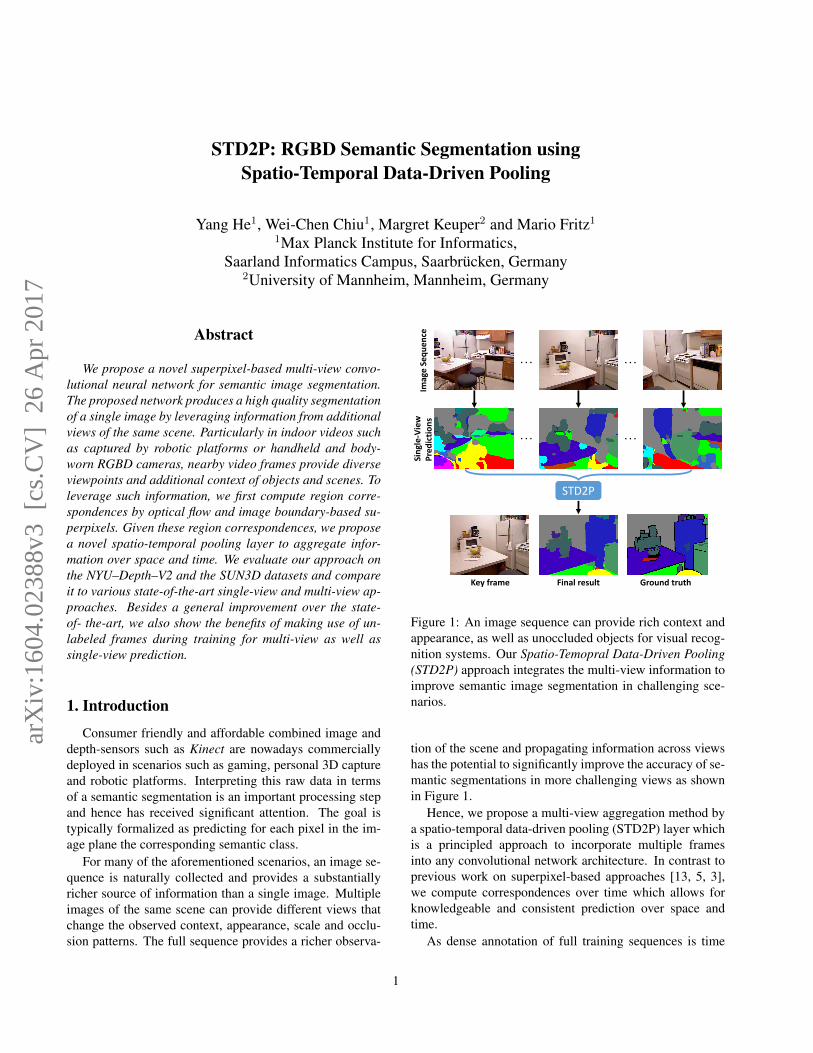
with the highest matching score if Rt has several successfulmatches. We show the statistics of region correspondenceson the NYUDv2 dataset in Figure 3.

It shows that 87.17% of the regions are relatively small(less than 2000 pixels) The plot on the right shows that thosesmall regions generally only find less than 10 matches ina whole video. Contrariwise, even slightly bigger regions

3

2k 4k 6k 8k 10k12k14k16k18k20k >22kNumber of pixels

0

100

101

102

Perc

en

tag

e

87.17

5.6

2.26

1.21

0.770.52

0.40.22 0.22 0.19

1.31

2k 4k 6k 8k 10k12k14k16k18k20k >22kNumber of pixels

0

10

20

30

40

50

60

Matc

hin

g N

um

ber

8.5

39.79

45.548.0

50.052.5 52.8

56.754.5

57.8 58.4

Figure 3: Statistics of region correspondences on theNYUDv2 dataset. (left) Distribution of region sizes; (right)Histogram of the average number of matches over regionsizes.

can be matched more easily and they cover large portionsof images. They usually have more than 40 matches in awhole video, and thus provide adequate information for ourmulti-view network.

3.2. Spatio-Temporal Data-Driven Pooling (STD2P)

Here, we describe our Spatio-Temporal Data-DrivenPooling (STD2P) model that uses the spatio-temporal struc-ture of the computed region correspondences to aggregateinformation across views as illustrated in Figure 2. Whilethe proposed method is highly compatible with recent CNNand FCN models, we build on a per frame model using [28].In more detail, we refine the output of the deconvolutionlayer with superpixels and aggregate the information frommultiple views by three layers: a spatial pooling layer, atemporal pooling layer and a region-to-pixel layer.

Spatial pooling layer. The input to the spatial poolinglayer is a feature map Is ∈ RN×C×H×W for N frames,C channels with size H × W and a superpixel map S ∈RN×H×W encoded with the region index. It generates theoutput Os ∈ RN×C×P , where P is the maximum num-ber of superpixels. The superpixel map S guides the for-ward and backward propagation of the layer. Here, Ωij =(x, y)|S(i, x, y) = j denotes a superpixel in the i-thframe with region index j. Then, the forward propagationof spatial average pooling can be formulated as

Os(i, c, j) =1

|Ωij |∑

(x,y)∈Ωij

Is(i, c, x, y) (1)

for each channel index c of the i-th frame and region in-dex j. We train our model using stochastic gradient de-scent. The gradient of the input Is(i, c, x, y), where (x, y) ∈Ωij , in our spatial pooling is calculated by back propaga-tion [34],

∂L

∂Is(i, c, x, y)=

∂L

∂Os(i, c, j)

∂Os(i, c, j)

∂Is(i, c, x, y)

=1

|Ωij |∂L

∂Os(i, c, j).

(2)

Temporal pooling layer. Similarly, we formulate ourtemporal pooling which fuses the information from Nframes It ∈ RN×C×P , which is the output of spatial pool-ing layer, to one frame Ot ∈ RC×P . This layer also needssuperpixel information Ωij , which is the superpixel with in-dex j of the i-th input frame. If Ωij 6= ∅, there existscorrespondence. The forward propagation can be expressedas

Ot(c, j) =1

K

∑Ωij 6=∅

It(i, c, j) (3)

for channel index c and region index j, where K =|i|Ωij 6= ∅, 1 ≤ i ≤ N|, which is the number of matchedframes for j-th region. The gradient is calculated by

∂L

∂It(i, c, j)=

∂L

∂Ot(c, j)

∂Ot(c, j)

∂It(i, c, j)

=1

K

∂L

∂Ot(c, j).

(4)

Region-to-pixel layer. To directly optimize a semanticsegmentation model with dense annotations, we map the re-gion based feature map Ir ∈ RC×P to a dense pixel-levelprediction Or ∈ RC×H×W . This layer needs a superpixelmap on the target frame Starget ∈ RH×W to perform for-ward and backward propagation. The forward propagationis expressed as

Or(c, x, y) = Ir(c, j), Starget(x, y) = j. (5)

The gradient is computed by

∂L

∂Ir(c, j)=

∑Starget(x,y)=j

∂L

∂Or(c, x, y)

∂Or(c, x, y)

∂Ir(c, j)

=∑

Starget(x,y)=j

∂L

∂Or(c, x, y).

(6)

4

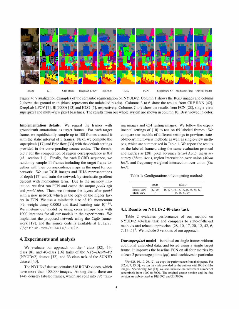
Image GT CRF-RNN DeepLab-LFOV BI(3000) E2S2 FCN Singleview SP Multiview Pixel Our full model

Figure 4: Visualization examples of the semantic segmentation on NYUDv2. Column 1 shows the RGB images and column2 shows the ground truth (black represents the unlabeled pixels). Columns 3 to 6 show the results from CRF-RNN [42],DeepLab-LFOV [7], BI(3000) [13] and E2S2 [5], respectively. Columns 7 to 9 show the results from FCN [28], single-viewsuperpixel and multi-view pixel baselines. The results from our whole system are shown in column 10. Best viewed in color.

Implementation details. We regard the frames withgroundtruth annotations as target frames. For each targetframe, we equidistantly sample up to 100 frames around itwith the static interval of 3 frames. Next, we compute thesuperpixels [17] and Epic flow [33] with the default settingsprovided in the corresponding source codes. The thresh-old τ for the computation of region correspondence is 0.4(cf. section 3.1). Finally, for each RGBD sequence, werandomly sample 11 frames including the target frame to-gether with their correspondence maps as the input for ournetwork. We use RGB images and HHA representationsof depth [17] and train the network by stochastic gradientdescent with momentum term. Due to the memory lim-itation, we first run FCN and cache the output pool4 rgband pool4 hha. Then, we finetune the layers after pool4with a new network which is the copy of the higher lay-ers in FCN. We use a minibatch size of 10, momentum0.9, weight decay 0.0005 and fixed learning rate 10−14.We finetune our model by using cross entropy loss with1000 iterations for all our models in the experiments. Weimplement the proposed network using the Caffe frame-work [19], and the source code is available at https://github.com/SSAW14/STD2P.

4. Experiments and analysis

We evaluate our approach on the 4-class [32], 13-class [8], and 40-class [16] tasks of the NYU–Depth–V2(NYUDv2) dataset [32], and 33-class task of the SUN3Ddataset [40].

The NYUDv2 dataset contains 518 RGBD videos, whichhave more than 400,000 images. Among them, there are1449 densely labeled frames, which are split into 795 train-

ing images and 654 testing images. We follow the exper-imental settings of [10] to test on 65 labeled frames. Wecompare our models of different settings to previous state-of-the-art multi-view methods as well as single-view meth-ods, which are summarized in Table 1. We report the resultson the labeled frames, using the same evaluation protocoland metrics as [28], pixel accuracy (Pixel Acc.), mean ac-curacy (Mean Acc.), region intersection over union (MeanIoU), and frequency weighted intersection over union (f.w.IoU).

Table 1: Configurations of competing methods

RGB RGBD

Single-View [12, 20] [5, 6, 7, 10, 13, 17, 28, 38, 39, 42]Multi-View / [8, 18, 37, 29]

4.1. Results on NYUDv2 40-class task

Table 2 evaluates performance of our method onNYUDv2 40-class task and compares to state-of-the-artmethods and related approaches [28, 10, 17, 20, 12, 42, 6,7, 13, 5] 1. We include 3 versions of our approach:

Our superpixel model is trained on single frames withoutadditional unlabeled data, and tested using a single targetframe. It improves the baseline FCN on all four metrics byat least 2 percentage points (pp), and it achieves in particular

1For [28, 10, 17, 20, 12], we copy the performance from their paper. For[42, 6, 7, 13, 5], we run the code provided by the authors with RGB+HHAimages. Specifically, for [13], we also increase the maximum number ofsuperpixels from 1000 to 3000. The original coarse version and the fineversion are abbreviated as BI(1000) and BI(3000).

5

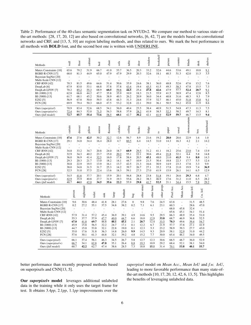
Table 2: Performance of the 40-class semantic segmentation task on NYUDv2. We compare our method to various state-of-the-art methods: [28, 17, 20, 12] are also based on convolutional networks, [6, 42, 7] are the models based on convolutionalnetworks and CRF, and [13, 5, 10] are region labeling methods, and thus related to ours. We mark the best performance inall methods with BOLD font, and the second best one is written with UNDERLINE.

Methods wal

l

floor

cabi

net

bed

chai

r

sofa

tabl

e

door

win

dow

book

shel

f

pict

ure

coun

ter

blin

ds

desk

shel

ves

Mutex Constraints [10] 65.6 79.2 51.9 66.7 41.0 55.7 36.5 20.3 33.2 32.6 44.6 53.6 49.1 10.8 9.1RGBD R-CNN [17] 68.0 81.3 44.9 65.0 47.9 47.9 29.9 20.3 32.6 18.1 40.3 51.3 42.0 11.3 3.5Bayesian SegNet [20] - - - - - - - - - - - - - - -Multi-Scale CNN [12] - - - - - - - - - - - - - - -CRF-RNN [42] 70.3 81.5 49.6 64.6 51.4 50.6 35.9 24.6 38.1 36.0 48.8 52.6 47.6 13.2 7.6DeepLab [6] 67.9 83.0 53.1 66.8 57.8 57.8 43.4 19.4 45.5 41.5 49.3 58.3 47.8 15.5 7.3DeepLab-LFOV [7] 70.2 85.2 55.3 68.9 60.5 59.8 44.5 25.4 47.8 42.6 47.9 57.7 52.4 20.7 9.1BI (1000) [13] 62.8 66.8 44.2 47.7 35.8 35.9 10.9 18.3 21.5 35.9 41.5 30.9 47.4 12.8 8.5BI (3000) [13] 61.7 68.1 45.2 50.6 38.9 40.3 26.2 20.9 36.0 34.4 40.8 31.6 48.3 9.3 7.9E2S2 [5] 56.9 67.8 50.0 59.5 43.8 44.3 31.3 24.6 37.9 32.7 46.1 45.0 51.8 15.8 9.1FCN [28] 69.9 79.4 50.3 66.0 47.5 53.2 32.8 22.1 39.0 36.1 50.5 54.2 45.8 11.9 8.6

Ours (superpixel) 70.9 83.4 52.6 68.5 54.1 56.0 40.4 25.5 38.4 40.9 51.5 54.8 47.3 11.3 7.5Ours (superpixel+) 72.4 84.3 52.0 71.5 54.3 58.8 37.9 28.2 41.9 38.5 52.3 58.2 49.7 14.3 8.1Ours (full model) 72.7 85.7 55.4 73.6 58.5 60.1 42.7 30.2 42.1 41.9 52.9 59.7 46.7 13.5 9.4

Methods curt

ain

dres

ser

pillo

w

mir

ror

floor

mat

clot

hes

ceili

ng

book

s

frid

ge

tv pape

r

tow

el

show

ercu

rtai

n

box

whi

tebo

ard

Mutex Constraints [10] 47.6 27.6 42.5 30.2 32.7 12.6 56.7 8.9 21.6 19.2 28.0 28.6 22.9 1.6 1.0RGBD R-CNN [17] 29.1 34.8 34.4 16.4 28.0 4.7 60.5 6.4 14.5 31.0 14.3 16.3 4.2 2.1 14.2Bayesian SegNet [20] - - - - - - - - - - - - - - -Multi-Scale CNN [12] - - - - - - - - - - - - - - -CRF-RNN [42] 34.8 33.2 34.7 20.8 24.0 18.7 60.9 29.5 31.2 41.1 18.2 25.6 23.0 7.4 13.9DeepLab [6] 32.9 34.3 40.2 23.7 15.0 20.2 55.1 22.1 30.6 49.4 21.8 32.1 6.4 5.8 14.8DeepLab-LFOV [7] 36.0 36.9 41.4 32.5 16.0 17.8 58.4 20.5 45.1 48.0 21.0 41.5 9.4 8.0 14.3BI (1000) [13] 29.3 20.3 21.7 13.0 18.2 14.1 44.7 10.9 21.5 30.4 18.8 22.3 17.7 5.5 12.4BI (3000) [13] 30.8 22.9 19.5 13.9 16.1 13.7 42.5 21.3 16.6 30.9 14.9 23.3 17.8 3.3 9.9E2S2 [5] 38.0 34.8 31.5 31.7 25.3 14.2 39.7 26.7 27.1 35.2 17.8 21.0 19.9 7.4 36.9FCN [28] 32.5 31.0 37.5 22.4 13.6 18.3 59.1 27.3 27.0 41.9 15.9 26.1 14.1 6.5 12.9

Ours (superpixel) 34.5 41.6 37.7 20.1 15.9 20.1 56.8 28.8 23.8 51.8 19.1 26.6 29.3 6.8 4.7Ours (superpixel+) 42.9 35.9 40.8 27.7 31.9 19.3 55.6 28.2 38.3 46.9 17.6 31.2 11.0 6.5 28.2Ours (full model) 40.7 44.1 42.0 34.5 35.6 22.2 55.9 29.8 41.7 52.5 21.1 34.4 15.5 7.8 29.2

Methods pers

on

nigh

tsta

nd

toile

t

sink

lam

p

bath

tub

bag

othe

rstr

uct

othe

rfur

ni

othe

rpro

ps

Pixe

lAcc

.

Mea

nA

cc.

Mea

nIo

U

f.w.I

oUMutex Constraints [10] 9.6 30.6 48.4 41.8 28.1 27.6 0 9.8 7.6 24.5 63.8 - 31.5 48.5RGBD R-CNN [17] 0.2 27.2 55.1 37.5 34.8 38.2 0.2 7.1 6.1 23.1 60.3 - 28.6 47.0Bayesian SegNet [20] - - - - - - - - - - 68.0 45.8 32.4 -Multi-Scale CNN [12] - - - - - - - - - - 65.6 45.1 34.1 51.4CRF-RNN [42] 57.9 31.4 57.2 45.4 36.9 39.1 4.9 14.6 9.5 29.5 66.3 48.9 35.4 51.0DeepLab [6] 55.3 37.7 57.9 47.7 40.0 44.7 6.6 18.0 12.9 33.8 68.7 46.9 36.8 52.5DeepLab-LFOV [7] 67.0 41.8 69.7 46.8 40.1 45.1 2.1 20.7 12.4 33.5 70.3 49.6 39.4 54.7BI (1000) [13] 45.9 15.8 56.5 32.2 24.7 17.1 0.1 12.2 6.7 21.9 57.7 37.8 27.1 41.9BI (3000) [13] 44.7 15.8 53.8 32.1 22.8 19.0 0.1 12.3 5.3 23.2 58.9 39.3 27.7 43.0E2S2 [5] 35.0 17.6 31.8 36.3 14.8 26.0 9.9 14.5 9.3 20.9 58.1 52.9 31.0 44.2FCN [28] 57.6 30.1 61.3 44.8 32.1 39.2 4.8 15.2 7.7 30.0 65.4 46.1 34.0 49.5

Ours (superpixel) 66.1 37.4 56.1 46.3 34.5 26.7 5.8 12.7 12.3 30.6 68.5 48.7 36.0 52.9Ours (superpixel+) 66.7 34.1 62.8 47.8 35.1 26.4 8.8 19.3 10.9 29.2 68.4 52.1 38.1 54.0Ours (full model) 60.7 42.2 62.7 47.4 38.6 28.5 7.3 18.8 15.1 31.4 70.1 53.8 40.1 55.7

better performance than recently proposed methods basedon superpixels and CNN[13, 5].

Our superpixel+ model leverages additional unlabeleddata in the training while it only uses the target frame fortest. It obtains 3.4pp, 2.1pp, 1.1pp improvements over the

superpixel model on Mean Acc., Mean IoU and f.w. IoU,leading to more favorable performance than many state-of-the-art methods [10, 17, 20, 12, 42, 6, 13, 5]. This highlightsthe benefits of leveraging unlabeled data.

6

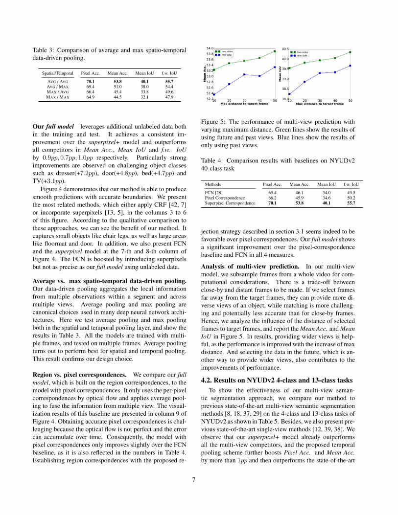
Table 3: Comparison of average and max spatio-temporaldata-driven pooling.

Spatial/Temporal Pixel Acc. Mean Acc. Mean IoU f.w. IoU

AVG / AVG 70.1 53.8 40.1 55.7AVG / MAX 69.4 51.0 38.0 54.4MAX / AVG 66.4 45.4 33.8 49.6MAX / MAX 64.9 44.5 32.1 47.9

Our full model leverages additional unlabeled data bothin the training and test. It achieves a consistent im-provement over the superpixel+ model and outperformsall competitors in Mean Acc., Mean IoU and f.w. IoUby 0.9pp, 0.7pp, 1.0pp respectively. Particularly strongimprovements are observed on challenging object classessuch as dresser(+7.2pp), door(+4.8pp), bed(+4.7pp) andTV(+3.1pp).

Figure 4 demonstrates that our method is able to producesmooth predictions with accurate boundaries. We presentthe most related methods, which either apply CRF [42, 7]or incorporate superpixels [13, 5], in the columns 3 to 6of this figure. According to the qualitative comparison tothese approaches, we can see the benefit of our method. Itcaptures small objects like chair legs, as well as large areaslike floormat and door. In addition, we also present FCNand the superpixel model at the 7-th and 8-th column ofFigure 4. The FCN is boosted by introducing superpixelsbut not as precise as our full model using unlabeled data.

Average vs. max spatio-temporal data-driven pooling.Our data-driven pooling aggregates the local informationfrom multiple observations within a segment and acrossmultiple views. Average pooling and max pooling arecanonical choices used in many deep neural network archi-tectures. Here we test average pooling and max poolingboth in the spatial and temporal pooling layer, and show theresults in Table 3. All the models are trained with multi-ple frames, and tested on multiple frames. Average poolingturns out to perform best for spatial and temporal pooling.This result confirms our design choice.

Region vs. pixel correspondences. We compare our fullmodel, which is built on the region correspondences, to themodel with pixel correspondences. It only uses the per-pixelcorrespondences by optical flow and applies average pool-ing to fuse the information from multiple view. The visual-ization results of this baseline are presented in column 9 ofFigure 4. Obtaining accurate pixel correspondences is chal-lenging because the optical flow is not perfect and the errorcan accumulate over time. Consequently, the model withpixel correspondences only improves slightly over the FCNbaseline, as it is also reflected in the numbers in Table 4.Establishing region correspondences with the proposed re-

10 20 30 40 50Max distance to target frame

52.2

52.4

52.6

52.8

53.0

53.2

53.4

53.6

53.8

54.0

Mean

Acc.

two sides

one side

10 20 30 40 50Max distance to target frame

38.0

38.5

39.0

39.5

40.0

40.5

Mean

IoU

two sides

one side

Figure 5: The performance of multi-view prediction withvarying maximum distance. Green lines show the results ofusing future and past views. Blue lines show the results ofonly using past views.

Table 4: Comparison results with baselines on NYUDv240-class task

Methods Pixel Acc. Mean Acc. Mean IoU f.w. IoU

FCN [28] 65.4 46.1 34.0 49.5Pixel Correspondence 66.2 45.9 34.6 50.2Superpixel Correspondence 70.1 53.8 40.1 55.7

jection strategy described in section 3.1 seems indeed to befavorable over pixel correspondences. Our full model showsa significant improvement over the pixel-correspondencebaseline and FCN in all 4 measures.

Analysis of multi-view prediction. In our multi-viewmodel, we subsample frames from a whole video for com-putational considerations. There is a trade-off betweenclose-by and distant frames to be made. If we select framesfar away from the target frames, they can provide more di-verse views of an object, while matching is more challeng-ing and potentially less accurate than for close-by frames.Hence, we analyze the influence of the distance of selectedframes to target frames, and report the Mean Acc. and MeanIoU in Figure 5. In results, providing wider views is help-ful, as the performance is improved with the increase of maxdistance. And selecting the data in the future, which is an-other way to provide wider views, also contributes to theimprovements of performance.

4.2. Results on NYUDv2 4-class and 13-class tasksTo show the effectiveness of our multi-view seman-

tic segmentation approach, we compare our method toprevious state-of-the-art multi-view semantic segmentationmethods [8, 18, 37, 29] on the 4-class and 13-class tasks ofNYUDv2 as shown in Table 5. Besides, we also present pre-vious state-of-the-art single-view methods [12, 39, 38]. Weobserve that our superpixel+ model already outperformsall the multi-view competitors, and the proposed temporalpooling scheme further boosts Pixel Acc. and Mean Acc.by more than 1pp and then outperforms the state-of-the-art

7

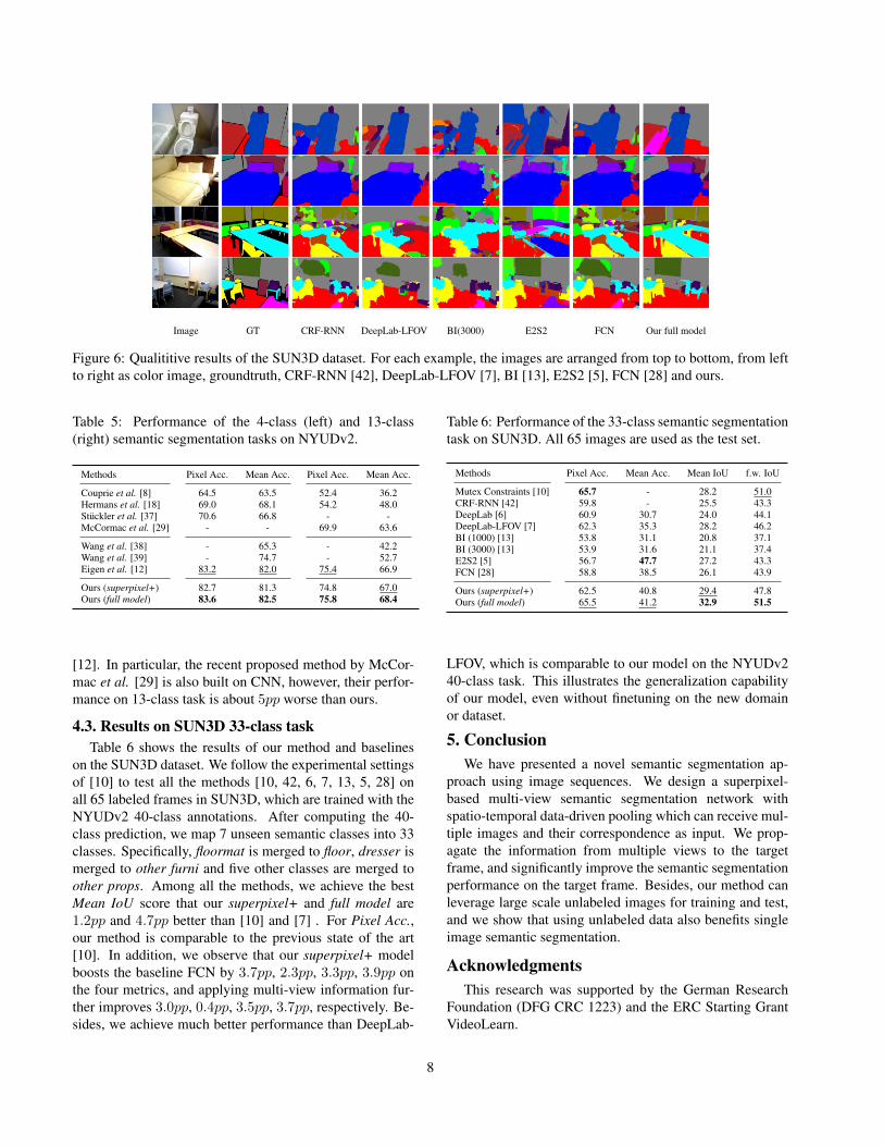
Image GT CRF-RNN DeepLab-LFOV BI(3000) E2S2 FCN Our full model

Figure 6: Qualititive results of the SUN3D dataset. For each example, the images are arranged from top to bottom, from leftto right as color image, groundtruth, CRF-RNN [42], DeepLab-LFOV [7], BI [13], E2S2 [5], FCN [28] and ours.

Table 5: Performance of the 4-class (left) and 13-class(right) semantic segmentation tasks on NYUDv2.

Methods Pixel Acc. Mean Acc. Pixel Acc. Mean Acc.

Couprie et al. [8] 64.5 63.5 52.4 36.2Hermans et al. [18] 69.0 68.1 54.2 48.0Stuckler et al. [37] 70.6 66.8 - -McCormac et al. [29] - - 69.9 63.6

Wang et al. [38] - 65.3 - 42.2Wang et al. [39] - 74.7 - 52.7Eigen et al. [12] 83.2 82.0 75.4 66.9

Ours (superpixel+) 82.7 81.3 74.8 67.0Ours (full model) 83.6 82.5 75.8 68.4

[12]. In particular, the recent proposed method by McCor-mac et al. [29] is also built on CNN, however, their perfor-mance on 13-class task is about 5pp worse than ours.

4.3. Results on SUN3D 33-class taskTable 6 shows the results of our method and baselines

on the SUN3D dataset. We follow the experimental settingsof [10] to test all the methods [10, 42, 6, 7, 13, 5, 28] onall 65 labeled frames in SUN3D, which are trained with theNYUDv2 40-class annotations. After computing the 40-class prediction, we map 7 unseen semantic classes into 33classes. Specifically, floormat is merged to floor, dresser ismerged to other furni and five other classes are merged toother props. Among all the methods, we achieve the bestMean IoU score that our superpixel+ and full model are1.2pp and 4.7pp better than [10] and [7] . For Pixel Acc.,our method is comparable to the previous state of the art[10]. In addition, we observe that our superpixel+ modelboosts the baseline FCN by 3.7pp, 2.3pp, 3.3pp, 3.9pp onthe four metrics, and applying multi-view information fur-ther improves 3.0pp, 0.4pp, 3.5pp, 3.7pp, respectively. Be-sides, we achieve much better performance than DeepLab-

Table 6: Performance of the 33-class semantic segmentationtask on SUN3D. All 65 images are used as the test set.

Methods Pixel Acc. Mean Acc. Mean IoU f.w. IoU

Mutex Constraints [10] 65.7 - 28.2 51.0CRF-RNN [42] 59.8 - 25.5 43.3DeepLab [6] 60.9 30.7 24.0 44.1DeepLab-LFOV [7] 62.3 35.3 28.2 46.2BI (1000) [13] 53.8 31.1 20.8 37.1BI (3000) [13] 53.9 31.6 21.1 37.4E2S2 [5] 56.7 47.7 27.2 43.3FCN [28] 58.8 38.5 26.1 43.9

Ours (superpixel+) 62.5 40.8 29.4 47.8Ours (full model) 65.5 41.2 32.9 51.5

LFOV, which is comparable to our model on the NYUDv240-class task. This illustrates the generalization capabilityof our model, even without finetuning on the new domainor dataset.

5. ConclusionWe have presented a novel semantic segmentation ap-

proach using image sequences. We design a superpixel-based multi-view semantic segmentation network withspatio-temporal data-driven pooling which can receive mul-tiple images and their correspondence as input. We prop-agate the information from multiple views to the targetframe, and significantly improve the semantic segmentationperformance on the target frame. Besides, our method canleverage large scale unlabeled images for training and test,and we show that using unlabeled data also benefits singleimage semantic segmentation.

AcknowledgmentsThis research was supported by the German Research

Foundation (DFG CRC 1223) and the ERC Starting GrantVideoLearn.

8

References[1] P. Arbelaez, B. Hariharan, C. Gu, S. Gupta, L. Bourdev, and

J. Malik. Semantic segmentation using regions and parts. InCVPR, 2012.

[2] P. Arbelaez, M. Maire, C. Fowlkes, and J. Malik. Contour de-tection and hierarchical image segmentation. TPAMI, 2011.

[3] A. Arnab, S. Jayasumana, S. Zheng, and P. H. Torr. Higherorder conditional random fields in deep neural networks. InECCV, 2016.

[4] W. Byeon, T. M. Breuel, F. Raue, and M. Liwicki. Scene la-beling with lstm recurrent neural networks. In CVPR, 2015.

[5] H. Caesar, J. Uijlings, and V. Ferrari. Region-based semanticsegmentation with end-to-end training. In ECCV, 2016.

[6] L.-C. Chen, G. Papandreou, I. Kokkinos, K. Murphy, andA. L. Yuille. Semantic image segmentation with deep con-volutional nets and fully connected crfs. In ICLR, 2014.

[7] L.-C. Chen, G. Papandreou, I. Kokkinos, K. Murphy, andA. L. Yuille. Deeplab: Semantic image segmentation withdeep convolutional nets, atrous convolution, and fully con-nected crfs. arXiv preprint arXiv:1606.00915, 2016.

[8] C. Couprie, C. Farabet, L. Najman, and Y. LeCun. Indoorsemantic segmentation using depth information. In ICLR,2013.

[9] J. Dai, K. He, and J. Sun. Convolutional feature masking forjoint object and stuff segmentation. In CVPR, 2015.

[10] Z. Deng, S. Todorovic, and L. Jan Latecki. Semantic seg-mentation of rgbd images with mutex constraints. In CVPR,2015.

[11] P. Dollar and C. Zitnick. Structured forests for fast edge de-tection. In CVPR, 2013.

[12] D. Eigen and R. Fergus. Predicting depth, surface normalsand semantic labels with a common multi-scale convolu-tional architecture. In ICCV, 2015.

[13] R. Gadde, V. Jampani, M. Kiefel, and P. V. Gehler. Super-pixel convolutional networks using bilateral inceptions. InECCV, 2016.

[14] F. Galasso, N. S. Nagaraja, T. J. Cardenas, T. Brox, andB. Schiele. A unified video segmentation benchmark: An-notation, metrics and analysis. In ICCV, 2013.

[15] M. Grundmann, V. Kwatra, M. Han, and I. Essa. Efficient hi-erarchical graph based video segmentation. In CVPR, 2010.

[16] S. Gupta, P. Arbelaez, and J. Malik. Perceptual organiza-tion and recognition of indoor scenes from rgb-d images. InCVPR, 2013.

[17] S. Gupta, R. Girshick, P. Arbelaez, and J. Malik. Learningrich features from rgb-d images for object detection and seg-mentation. In ECCV. 2014.

[18] A. Hermans, G. Floros, and B. Leibe. Dense 3d semanticmapping of indoor scenes from rgb-d images. In ICRA, 2014.

[19] Y. Jia, E. Shelhamer, J. Donahue, S. Karayev, J. Long, R. Gir-shick, S. Guadarrama, and T. Darrell. Caffe: Convolutionalarchitecture for fast feature embedding. In ACM Multimedia,2014.

[20] A. Kendall, B. Vijay, and R. Cipolla. Bayesian segnet:Model uncertainty in deep convolutional encoder-decoderarchitectures for scene understanding. arXiv preprintarXiv:1511.02680, 2015.

[21] A. Krizhevsky, I. Sutskever, and G. E. Hinton. Imagenetclassification with deep convolutional neural networks. InNIPS, 2012.

[22] A. Kundu, V. Vineet, and V. Koltun. Feature space optimiza-tion for semantic video segmentation. In CVPR, 2016.

[23] Z. Li, Y. Gan, X. Liang, Y. Yu, H. Cheng, and L. Lin. Lstm-cf: Unifying context modeling and fusion with lstms for rgb-d scene labeling. In ECCV, 2016.

[24] G. Lin, C. Shen, I. Reid, et al. Efficient piecewise training ofdeep structured models for semantic segmentation. In CVPR,2015.

[25] M. Lin, Q. Chen, and S. Yan. Network in network. In ICLR,2014.

[26] W. Liu, A. Rabinovich, and A. C. Berg. Parsenet: Lookingwider to see better. arXiv preprint arXiv:1506.04579, 2015.

[27] Z. Liu, X. Li, P. Luo, C.-C. Loy, and X. Tang. Semantic im-age segmentation via deep parsing network. In ICCV, 2015.

[28] J. Long, E. Shelhamer, and T. Darrell. Fully convolutionalnetworks for semantic segmentation. In CVPR, 2015.

[29] J. McCormac, A. Handa, A. Davison, and S. Leutenegger.Semanticfusion: Dense 3d semantic mapping with convo-lutional neural networks. arXiv preprint arXiv:1609.05130,2016.

[30] R. Mottaghi, X. Chen, X. Liu, N.-G. Cho, S.-W. Lee, S. Fi-dler, R. Urtasun, and A. Yuille. The role of context for objectdetection and semantic segmentation in the wild. In CVPR,2014.

[31] S. K. Mustikovela, M. Y. Yang, and C. Rother. Can groundtruth label propagation from video help semantic segmenta-tion? ECCV Workshop on Video Segmentation, 2016.

[32] P. K. Nathan Silberman, Derek Hoiem and R. Fergus. Indoorsegmentation and support inference from rgbd images. InECCV, 2012.

[33] J. Revaud, P. Weinzaepfel, Z. Harchaoui, and C. Schmid.Epicflow: Edge-preserving interpolation of correspondencesfor optical flow. In CVPR, 2015.

[34] D. E. Rumelhart, G. E. Hinton, and R. J. Williams. Learningrepresentations by back-propagating errors. Cognitive mod-eling, 5(3):1, 1988.

[35] B. Shuai, Z. Zuo, G. Wang, and B. Wang. Dag-recurrentneural networks for scene labeling. In CVPR, 2016.

[36] K. Simonyan and A. Zisserman. Very deep convolutionalnetworks for large-scale image recognition. arXiv preprintarXiv:1409.1556, 2014.

[37] J. Stuckler, B. Waldvogel, H. Schulz, and S. Behnke. Densereal-time mapping of object-class semantics from rgb-dvideo. Journal of Real-Time Image Processing, 10(4), 2015.

[38] A. Wang, J. Lu, W. Gang, J. Cai, and T.-J. Cham. Multi-modal unsupervised feature learning for rgb-d scene label-ing. In ECCV, 2014.

[39] J. Wang, Z. Wang, D. Tao, S. See, and G. Wang. Learningcommon and specific features for rgb-d semantic segmenta-tion with deconvolutional networks. In ECCV, 2016.

[40] J. Xiao, A. Owens, and A. Torralba. Sun3d: A databaseof big spaces reconstructed using sfm and object labels. InICCV, 2013.

9

[41] F. Yu and V. Koltun. Multi-scale context aggregation by di-lated convolutions. In ICLR, 2016.

[42] S. Zheng, S. Jayasumana, B. Romera-Paredes, V. Vineet,Z. Su, D. Du, C. Huang, and P. Torr. Conditional randomfields as recurrent neural networks. In ICCV, 2015.

[43] B. Zhou, A. Khosla, L. A., A. Oliva, and A. Torralba. Learn-ing Deep Features for Discriminative Localization. In CVPR,2016.

10

Supplementary MaterialsA. Analysis of semantic segmentation boundary ac-

curacy

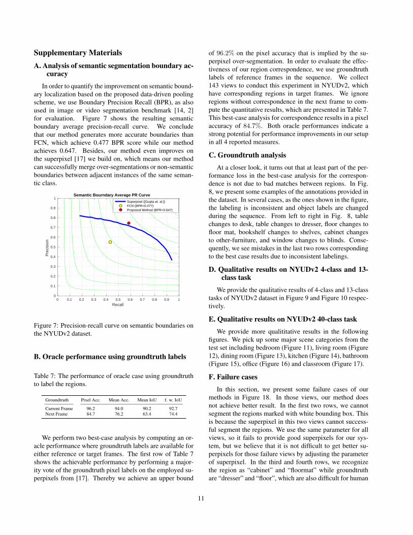
In order to quantify the improvement on semantic bound-ary localization based on the proposed data-driven poolingscheme, we use Boundary Precision Recall (BPR), as alsoused in image or video segmentation benchmark [14, 2]for evaluation. Figure 7 shows the resulting semanticboundary average precision-recall curve. We concludethat our method generates more accurate boundaries thanFCN, which achieve 0.477 BPR score while our methodachieves 0.647. Besides, our method even improves onthe superpixel [17] we build on, which means our methodcan successfully merge over-segmentations or non-semanticboundaries between adjacent instances of the same seman-tic class.

0 0.1 0.2 0.3 0.4 0.5 0.6 0.7 0.8 0.9 1

Recall

0

0.1

0.2

0.3

0.4

0.5

0.6

0.7

0.8

0.9

1

Pre

cisi

on

Semantic Bourndary Average PR Curve

Superpixel ([Gupta et. al.])FCN (BPR=0.477)Proposed Method (BPR=0.647)

Figure 7: Precision-recall curve on semantic boundaries onthe NYUDv2 dataset.

B. Oracle performance using groundtruth labels

Table 7: The performance of oracle case using groundtruthto label the regions.

Groundtruth Pixel Acc. Mean Acc. Mean IoU f. w. IoU

Current Frame 96.2 94.0 90.2 92.7Next Frame 84.7 76.2 63.4 74.4

We perform two best-case analysis by computing an or-acle performance where groundtruth labels are available foreither reference or target frames. The first row of Table 7shows the achievable performance by performing a major-ity vote of the groundtruth pixel labels on the employed su-perpixels from [17]. Thereby we achieve an upper bound

of 96.2% on the pixel accuracy that is implied by the su-perpixel over-segmentation. In order to evaluate the effec-tiveness of our region correspondence, we use groundtruthlabels of reference frames in the sequence. We collect143 views to conduct this experiment in NYUDv2, whichhave corresponding regions in target frames. We ignoreregions without correspondence in the next frame to com-pute the quantitative results, which are presented in Table 7.This best-case analysis for correspondence results in a pixelaccuracy of 84.7%. Both oracle performances indicate astrong potential for performance improvements in our setupin all 4 reported measures.

C. Groundtruth analysis

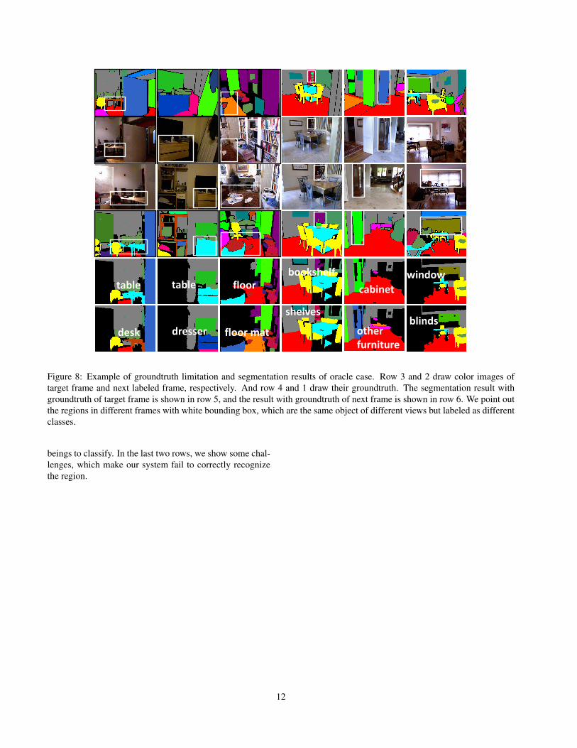
At a closer look, it turns out that at least part of the per-formance loss in the best-case analysis for the correspon-dence is not due to bad matches between regions. In Fig.8, we present some examples of the annotations provided inthe dataset. In several cases, as the ones shown in the figure,the labeling is inconsistent and object labels are changedduring the sequence. From left to right in Fig. 8, tablechanges to desk, table changes to dresser, floor changes tofloor mat, bookshelf changes to shelves, cabinet changesto other-furniture, and window changes to blinds. Conse-quently, we see mistakes in the last two rows correspondingto the best case results due to inconsistent labelings.

D. Qualitative results on NYUDv2 4-class and 13-class task

We provide the qualitative results of 4-class and 13-classtasks of NYUDv2 dataset in Figure 9 and Figure 10 respec-tively.

E. Qualitative results on NYUDv2 40-class task

We provide more qualititative results in the followingfigures. We pick up some major scene categories from thetest set including bedroom (Figure 11), living room (Figure12), dining room (Figure 13), kitchen (Figure 14), bathroom(Figure 15), office (Figure 16) and classroom (Figure 17).

F. Failure cases

In this section, we present some failure cases of ourmethods in Figure 18. In those views, our method doesnot achieve better result. In the first two rows, we cannotsegment the regions marked with white bounding box. Thisis because the superpixel in this two views cannot success-ful segment the regions. We use the same parameter for allviews, so it fails to provide good superpixels for our sys-tem, but we believe that it is not difficult to get better su-perpixels for those failure views by adjusting the parameterof superpixel. In the third and fourth rows, we recognizethe region as “cabinet” and “floormat” while groundtruthare “dresser” and “floor”, which are also difficult for human

11

table

desk

table floor

dresser

window

blinds shelves

floor mat

bookshelf

other furniture

cabinet

Figure 8: Example of groundtruth limitation and segmentation results of oracle case. Row 3 and 2 draw color images oftarget frame and next labeled frame, respectively. And row 4 and 1 draw their groundtruth. The segmentation result withgroundtruth of target frame is shown in row 5, and the result with groundtruth of next frame is shown in row 6. We point outthe regions in different frames with white bounding box, which are the same object of different views but labeled as differentclasses.

beings to classify. In the last two rows, we show some chal-lenges, which make our system fail to correctly recognizethe region.

12

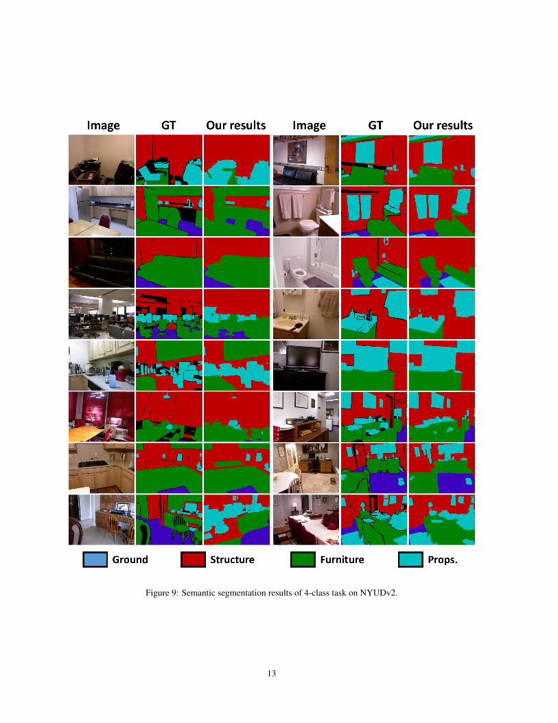
Figure 9: Semantic segmentation results of 4-class task on NYUDv2.

13

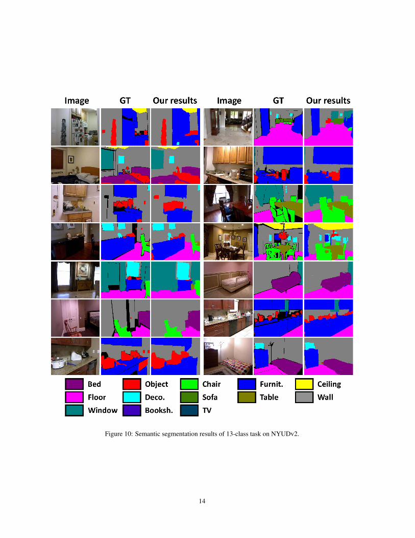
Figure 10: Semantic segmentation results of 13-class task on NYUDv2.

14

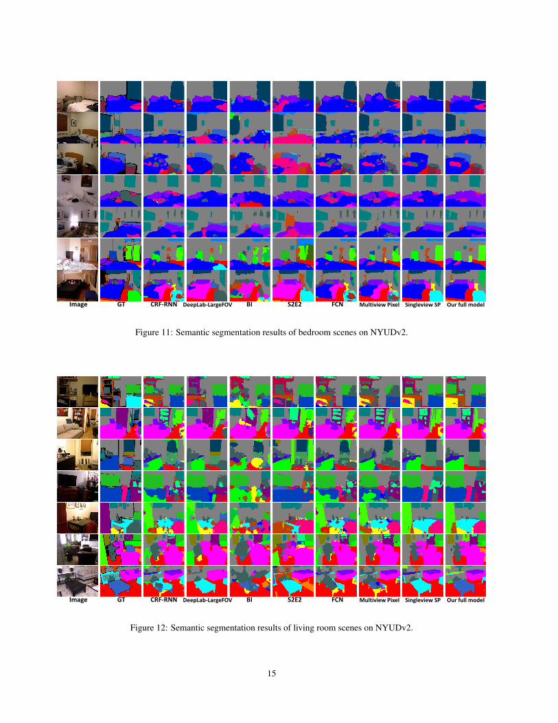
Image GT CRF-RNN DeepLab-LargeFOV BI S2E2 FCN Multiview Pixel Singleview SP Our full model

Figure 11: Semantic segmentation results of bedroom scenes on NYUDv2.

Image GT CRF-RNN DeepLab-LargeFOV BI S2E2 FCN Multiview Pixel Singleview SP Our full model

Figure 12: Semantic segmentation results of living room scenes on NYUDv2.

15

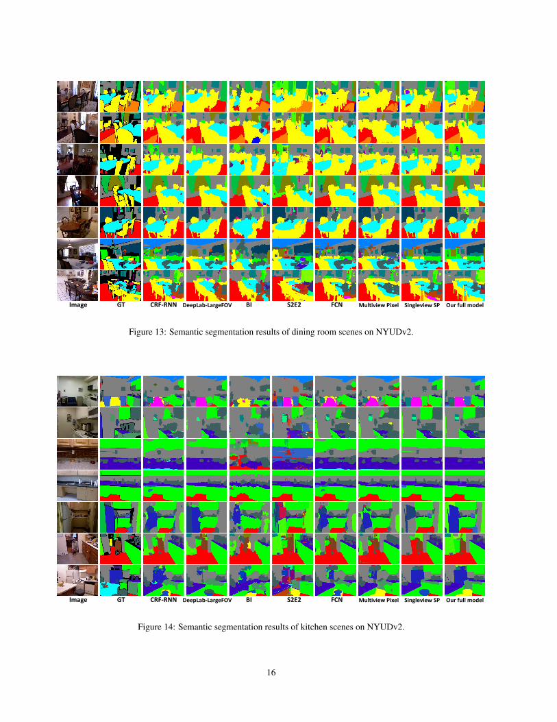
Image GT CRF-RNN DeepLab-LargeFOV BI S2E2 FCN Multiview Pixel Singleview SP Our full model

Figure 13: Semantic segmentation results of dining room scenes on NYUDv2.

Image GT CRF-RNN DeepLab-LargeFOV BI S2E2 FCN Multiview Pixel Singleview SP Our full model

Figure 14: Semantic segmentation results of kitchen scenes on NYUDv2.

16

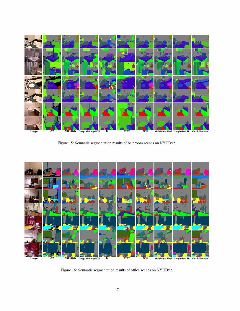
Image GT CRF-RNN DeepLab-LargeFOV BI S2E2 FCN Multiview Pixel Singleview SP Our full model

Figure 15: Semantic segmentation results of bathroom scenes on NYUDv2.

Image GT CRF-RNN DeepLab-LargeFOV BI S2E2 FCN Multiview Pixel Singleview SP Our full model

Figure 16: Semantic segmentation results of office scenes on NYUDv2.

17

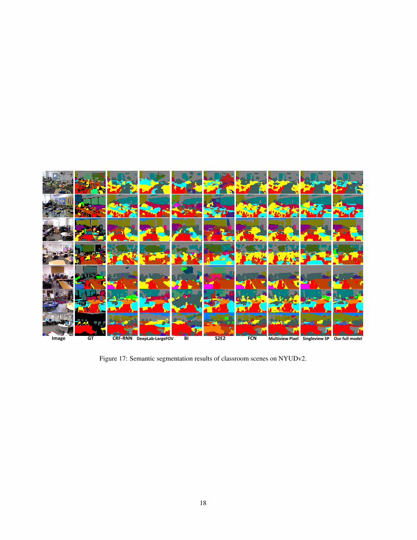
Image GT CRF-RNN DeepLab-LargeFOV BI S2E2 FCN Multiview Pixel Singleview SP Our full model

Figure 17: Semantic segmentation results of classroom scenes on NYUDv2.

18

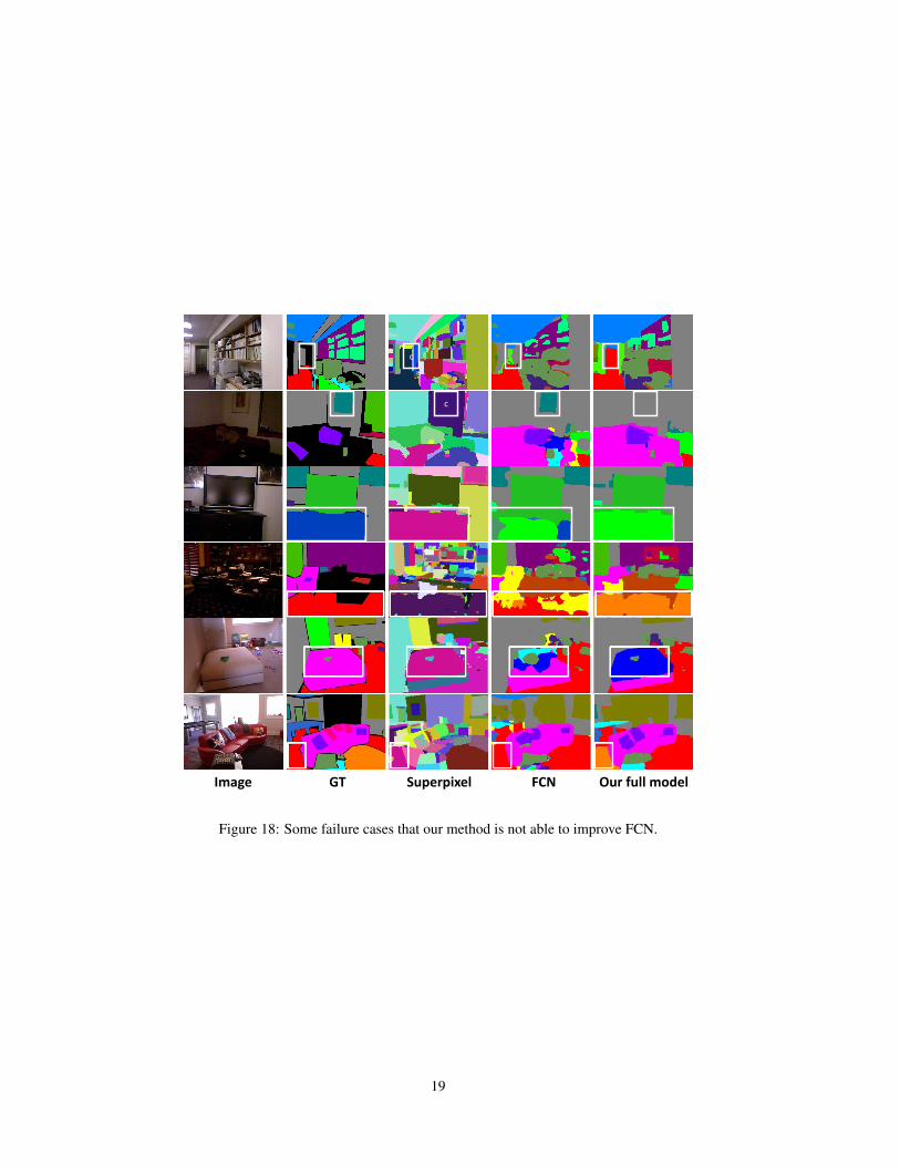
Image GT FCN Our full modelSuperpixel

c

c

Figure 18: Some failure cases that our method is not able to improve FCN.

19