Temperature and Productivity: Evidence from Plant-level Data

Temperature and Productivity: Evidence from Plant-level Data

Chen Chen, Thanh D. Huynh, and Bohui Zhang*

This Draft: April 2019

* For helpful comments, the authors would like to thank Stephen Brown, Ulrich Hege, Darwin Choi,

Fangjian Fu, Juhani Linnainmaa, and workshop participants at the CGKSB, the Renmin University, the

Fanhai International School of Finance, and the University of Nottingham Ningbo China. Chen Chen and

Thanh Huynh are from Monash Business School, Monash University, Caulfield East 3145, Australia and

Bohui Zhang is from School of Management and Economics and Shenzhen Finance Institute, The Chinese

University of Hong Kong, Shenzhen, 518172, China. Authors’ contact information: Chen:

[email protected], (61) 3-99032023; Huynh: [email protected], (61) 3-99031474, and

Zhang: [email protected].

mailto:[email protected]



1

Temperature and Productivity: Evidence from Plant-level Data

Abstract

Research in biomedical science finds that warmer temperature diminishes functioning of human

brains, causes stress and anxiety, affects people’s mood, and leads to higher suicide rate and

various social conflicts. Using plant-level data in the U.S., we find that on average warmer

temperature negatively affects plant’s productivity. The average effect of temperature remains

strong for plants that choose to relocate to warmer counties presumably for tax reasons, suggesting

that our results are robust to self-selection concerns. Using information on establishment-level

innovation, we document that warmer temperature affects the productivity of inventors and

contributes to the net outflows of inventors out of the county. We estimate county-level measures

of suicide rate-temperature sensitivity and hospital admissions-temperature sensitivity and find

that temperature affects productivity via its negative impacts on employees’ mental and physical

health. Placebo test shows an insignificant effect of weekend temperature on productivity,

suggesting that our results are not a spurious relation. This study contributes to the emerging

climate finance literature by documenting micro-level evidence on the impact of rising temperature

on plant-level productivity.

Keywords: Temperatures; Firm Performance; Plant-Level Productivity; Innovation; Mental

Health; Physical Health

JEL Code: G30; G38

2

“Don’t fall in to the trap of arguing whether climate change is real… The real debate is how much

economic damage does climate change actually do.”

John H. Cochrane (February 2017)

Former President of the American Finance Association

1. Introduction

Climate research documents that warming temperature has a negative impact on public health

(Deschênes and Greenstone, 2011), social unrest, violence, and human conflicts (Hsiang and

Burke, 2014). Recent studies (e.g., Hsiang, 2010; Dell, Jones, and Olken, 2012; Burke, Hsiang,

and Miguel, 2015) provide macro-level evidence that a country’s economic activities significantly

decline when its temperature increases. There is, however, little research on how rising

temperature affects productivity at the micro (i.e., establishment) level. Addressing this question

is important because business entities play a central role in driving a country’s productivity and

innovation. As the above quote pointed out, it also offers direct implications for corporate

managers, investors, and policymakers on the degree of economic damage that warming

temperature caused to businesses.

Building on research in the biomedical field, we hypothesize that temperature affects firm

performance via lower productivity of workers. Scientific research suggests that productivity is

lower because human bodies cannot cope with uncomfortable and hot temperature. When

employees’ productivity is lower, it follows that firm performance and productivity will suffer.

There are at least three medical reasons for lower employees’ performance as temperature is

warmer.

First, warm temperature ranging from 25 to 35°C (77-95°F) will cause heart rate to be higher

and heart rate variability (HRV) to be lower (Sollers et al., 2002; Wu et al., 2013), which are the

conditions leading to higher stress and anxiety. The physical effect is analogous to people facing

danger or harmful situations, which cause their HRV to be lower (Malik, 1996; Stauss, 2003;

3

Thayer et al., 2012). Low HRV is also an important determinant of bad mood, which Caplan and

Jones (1975) and Laborde and Raab (2013) show to negatively affect creativity, productivity, and

even decision making of people. Taken together, research in cardiology finds that higher

temperature affects HRV, which, in turn, negatively affects people’s mood, creativity, and

cognitive ability (Davis, 2009; Laborde and Raab, 2013).

Second, warmer temperature affects the ability of the brain to dispose of waste heat. When the

brain is overheated, its functions become significantly impaired. On average, the brain generates

20% of all the heat of the human body of which it needs to dispose. Since the brain’s functioning

is sensitive to temperature, the disposal of waste heat becomes harder when the ambient

temperature rises (Schiff and Somjen, 1985; Yablonskiy et al., 2000). Schiff and Somjen (1985),

for example, document that when ambient temperature ranges 29-33°C (84-91°F), there is an

elevated risk of dysfunctions of brain activities.

Third, human bodies devote more energy to cool down when the ambient temperature is hotter

than it does to warm up when the temperature is colder (Kilbourne, 1997; Parsons, 2003). When

temperature is high, the body automatically circulates more blood near the skin to take advantage

of cooling opportunities, thereby limiting the supply of blood to key organs, such as the brain and

the heart. Moreover, warmer temperature makes dehydration more likely, which diminishes

employees’ productivity (Sawka and Montain, 2000).

Building on the above scientific evidence, we hypothesize that, by affecting employees’

cognitive and physical activities, warm temperature can have a negative impact on business entities’

performance and productivity. Research in health economics suggests that ambient temperature

also has an impact on the productivity of office workers. Deryugina and Hsiang (2013) find that

the U.S. economy has not fully implemented adaptation measures to offset the impact of warming

4

temperature. They argue that, because the marginal cost of adaptation is sufficiently large, it is

optimal for economic activities to “not fully be insulated from the environment”. Indeed, while

many commercial buildings are air-conditioned, the internal thermal conditions are often either

not well-controlled or not adjusted as frequently as the outside temperature changes (Seppanen et

al. 2006). Federspiel et al. (2004) find that temperature can affect workers’ productivity because

employees typically cannot set their own thermostat to a comfortable level. Zivin et al. (2015)

track the performance of students in mathematics between 1979 and 1994 and find that these

students perform worse on warm days (greater than 26℃ or 78°F). In their study, students are

interviewed on randomly chosen days in their homes. This finding is consistent with the medical

findings that high temperature can affect the functioning of human brains, thereby impairing their

cognitive ability. Seppanen et al. (2006) examine the effect of temperature on productivity of call-

center workers and find that higher temperature causes longer customer service time and handling

time per customer call. Zivin and Neidell (2014) document that employees in the manufacturing

industry allocate less time to work on days when temperature is higher. Finally, even when

employees may stay indoor most of the time, they are still exposed to outdoor temperatures during

their commute.

To examine the effect of temperature on business entities’ productivity, we employ

comprehensive plant-level data on U.S. subsidiaries, branches, and plants from the National

Establishment Time Series (NETS) database over the period from 1990 to 2015. Using the

information on outputs and employment levels of plants from the NETS database, we compute

two alternate measures of plant-level productivity: total factor productivity (TFP), which captures

the overall productivity of a plant in utilizing its capital and labor, and the modified TFP measure,

OP_TFP, which is estimated using Olley and Pakes (1996) method. The latter measure corrects

5

for the possibility that plants simultaneously choose the level of inputs as they choose their outputs.

We obtain daily temperature data at the county level from the U.S. National Climatic Data Center

(NCDC) and compute a yearly temperature measure in the county of a plant as the average of daily

temperature over a firm’s fiscal year. To maintain the convention in both the NCDC database and

the vast majority of scientific studies, we measure temperature in degrees Celsius.

We find that warmer temperature causes both measures of TFP to be lower. The effect is strong

and robust even after controlling for a battery of known plant-level and firm-level characteristics,

county-level variables, as well as the inclusion of various fixed effects such as firm, county, and

year fixed effects or firm-by-year and county fixed effects. The effect is also economically

significant. For example, using the plant-level TFP as a measure of productivity, a 1°𝐶 (1.8°𝐹)

rise in the average yearly temperature is associated with a reduction of productivity by 8.9%

relative to the sample average (or equivalent to a drop from the 75𝑡ℎ percentile to the 60𝑡ℎ

percentile of productivity in the cross-section of plants).1 While the effect of temperature on

productivity is broadly manifested across industries in the U.S., the relation is, expectedly, stronger

for plants in agriculture and outdoor industries. At the firm level, we find that Tobin’s Q of multi-

state firms is significantly lower when temperatures in their plants’ local counties are warmer.2

While yearly variation in temperature is arguably exogenous to firm characteristics, the

location of a plant may not be random. To mitigate this concern, we take advantage of state-level

tax changes and analyze the productivity of plants that relocate from a colder, higher-tax county

to a hotter, lower-tax county. We contend that these plant relocations are possibly motivated by

lower corporate tax rates, since Giroud and Rauh (2018) find causal evidence that a decrease in

1 In Section 4, we replicate our main empirical results using firm-level Tobin’s Q and find that our results do not

qualitatively change. 2 We approximate the firm-level temperature by computing the weighted average of temperatures in the plants’

counties where the weight is the plant’s economic weight within the firm’s network.

6

state-level corporate tax rate leads to more new plants in the state. We conduct a difference-in-

difference analysis surrounding a plant’s relocation event within two years after the tax-reduction

law was passed. We find that treatment plants experience a significant drop in their productivity

compared to the other plants. In terms of economic magnitude, after relocating to a warmer county

treatment plants experience a reduction in TFP by 18-23% relative to the sample mean. These

results suggest that plants, which choose to relocate to a warmer county presumably for tax-

motivated purposes, are also affected by warmer temperature.

We next examine whether plant’s productivity is affected by warmer or colder temperatures.

We do so by constructing four variables representing the number of days over the firm’s fiscal

year in which the daily average temperature is below 10℃ (50℉), between 10℃ (50℉) and 20℃

(68℉), between 20℃ (68℉) and 30℃ (86℉), and above 30℃ (86℉). We find an inverted U-

shaped relation between temperature days and plant-level productivity. However, consistent with

scientific findings, the effect of Ln(> 30℃ days) is stronger and more robust than that of colder

temperatures. These results are consistent with the biomedical evidence that employees’ cognitive

and physical activities are significantly impaired when temperature is warmer.

A potential alternative explanation for our findings is that the effect of temperature on

establishment-level productivity may be driven by lower local customer demand, rather than lower

workers’ productivity. To rule out this alternative explanation, we follow Agrawal and Matsa

(2013) and employ data of total revenues of goods shipped to intrastate and interstate customers

from the US Commodity Flow Survey, which is conducted by the U.S. Bureau of the Census and

surveys plants across the U.S. We examine the effect of local temperature on productivity of a

sample of plants, whose 95% of sales revenues come from out-of-state customers. We continue to

7

find that these plants are negatively affected by their local counties’ temperatures. These results

indicate that demand of local customers is unlikely to be the explanation for our findings.

We perform several additional tests, which together suggest that temperature affects

establishment-level productivity via its impacts on the mental and physical activities of employees.

We first investigate the effect of temperature on corporate innovation (i.e., productivity of

inventors). We construct establishment-level innovation measures by merging the patent

information from Kogan et al. (2017) and the location of inventors of each patent from the U.S.

Patent Inventor Database. We find that both the number of patents and patent citations at each

establishment are lower as county’s temperature rises, suggesting that temperature affects

productivity via its negative impacts on the creativity and cognitive activities of inventors. We

further find that the effect of temperature is more pronounced for establishments, whose overall

productivity is more dependent on innovation outputs. At the aggregate county level, we show that

counties experience a significant net outflow of inventors when their medium- and long-run

temperatures increase.

In our next avenue of inquiry, we examine whether plant’s productivity is lower in counties,

whose residents’ mental health is more sensitive to warmer temperature. Research in

environmental and health economics finds that social conflicts are particularly responsive to

changes in temperature (Hsiang, Burke, and Miguel, 2013). Burke et al. (2018) document that

warm temperature leads to higher suicide rates in the U.S. and Mexico, indicating that high

temperature can have a negative impact on mental health. To the extent that local temperature

affects productivity via its negative impacts on the mental health of residents, we expect that

plant’s productivity is significantly lower in counties whose residents’ mental health is more

sensitive to warmer temperature. To test this conjecture, we estimate a yearly county-level measure

8

of sensitivity of suicide rates to temperature and examine the effect of this sensitivity on plant-

level productivity. Consistent with our hypothesis, we find that plant’s productivity is significantly

lower as county’s suicide rate sensitivity to temperature increases. This finding is consistent with

the notion that temperature affects firm performance by impairing mental health of workers and,

in turn, their productivity.

We further examine whether plant’s productivity is lower in counties, whose residents’

physical health is more sensitive to temperature. Employing data on hospital admissions in

California, we estimate a measure of county-level sensitivity of residents’ physical health to

temperature and examine the effect of this sensitivity on plant’s productivity. Consistent with our

hypothesis, we find that plant’s productivity is significantly lower in counties with high hospital

admissions-temperature sensitivity.3

Finally, we conduct a placebo analysis in which we test the effect of weekend temperature on

plant’s productivity and find that the effect is statistically insignificant. As most major business

operations occur on weekdays, rather than weekends (Deryugina and Hsiang, 2014), these results

suggest that the relation between temperature and firm performance documented in our study is

not a spurious result. In other robustness tests, we confirm that our results do not qualitatively

change when we examine the effect of long-run average temperature or when we control for other

weather-related variables such as sunshine, wind speed, precipitation, and air evaporation.

Our study contributes to the existing literature in two ways. First, we employ a comprehensive

plant-level dataset and provide one of the first micro-level evidence of the average effect of

temperature on plant-level productivity and firm performance in the U.S. There is a dearth of

empirical evidence on this important question. Burke, Hsiang, and Miguel (2015) provides macro-

3 We use California-based hospitals because only these admissions data are available to us. We confirm that our

baseline results are not driven by establishments in California.

9

level evidence by studying the data from 166 countries. Given that U.S. corporations have business

operations in multiple states, it remains unknown whether the average effect of temperature across

all establishments in the U.S. is consistent with the macro-level findings. Our study takes

advantage of presumably random fluctuations in daily temperatures at the county level in the U.S.

and document robust evidence that warm temperatures are detrimental to firm performance,

establishment productivity, and innovation. Moreover, we also find that temperature affects firm

performance by affecting employees’ mental and physical health – consistent with findings the

medical literature. As such, our study has direct implications for managers and policymakers.

This study also contributes to the emerging literature on climate finance, which is still limited

in scope and chiefly examines the impact of climate change in capital markets. Hong, Li, and Xu

(2018) investigate whether the market efficiently incorporates the risk of droughts in stock prices

of food companies. Bansal, Kiku, and Ochoa (2016) document that virtually all U.S. equity

portfolios are exposed to the risk of rising temperature. Choi, Gao, and Jiang (2018) find that

stocks of carbon-intensive firms experience a lower average return than those of low-carbon firms

in abnormally warm temperatures. Painter (2018) documents that counties affected by climate

change incur a higher cost of debt when issuing long-term municipal bonds compared to counties

unlikely to be affected by climate change. In the real estate market, Bernstein, Gustafson, and

Lewis (2017) find that prices of homes on the coastal lines that will be affected by rising sea levels

are sold at a discount compared to unaffected homes. Baldauf, Garlappi, and Yannelis (2018) show

that differences in beliefs about climate change in a neighborhood will determine house prices in

the area. Our study adds to this contemporary literature by documenting the real consequences of

rising temperature on the business entities’ performance and productivity.

10

The remainder of the paper is organized as follows. Section 2 describes the data and research

design. Section 3 shows the descriptive statistics and our main findings. Section 4 reports the

additional analysis and Section 5 concludes the paper.

2. Data

2.1. Plant-level and firm-level data

We obtain information on subsidiaries, branches, and plants of multi-state firms from the National

Establishment Time-Series (NETS) database between 1990 and 2015, which is supplied by credit

rating agency, Dun and Bradstreet (D&B), and is maintained by Walls and Associates.4 As noted

by Faccio and Hsu (2017), the NETS database contains a comprehensive record of plants in the

U.S. because plants wishing to obtain lines of credit from suppliers or financial institutions have

incentives to report accurate information. D&B also collects information from independent sources

including phone calls to suppliers and customers, legal and bankruptcy filings, press reports, and

government records (Heidi and Ljungqvist, 2015; Ljungqvist et al., 2017).

The NETS database provides us with information on the county, number of employees, and

sales at each establishment, as well as their historical headquarters’ names and locations. In our

regression tests, we control for plant-level credit score, Credit_Score, which ranges from 0 to 100

and is rated by D&B using the trade credit information supplied by suppliers and customers of a

plant. Following prior research (Heidi and Ljungqvist 2015; Ljungqvist et al. 2017), we match

plants in the NETS database with firms in Compustat by their legal names and historical

headquarters information obtained from their SEC filings. Our firm-level data are the intersection

4 Our sample period is constrained by the availability of the NETS database. At the time of conducting this study,

2015 is the latest update of the NETS database.

11

of accounting data from Compustat and market data from CRSP. As standard in the literature, we

do not consider financial firms (those with SIC codes 6000-6999) and non-common stocks (those

with CRSP share codes different from 10 or 11).

We employ two alternate proxies for plant-level performance: total factor productivity (TFP)

and the refined measure of TFP (OP_TFP) following the estimation method in Olley and Pakes

(1996). First, 𝑇𝐹𝑃 is a measure of overall productivity of a plant in utilizing its capital and labor

(e.g., Olley and Pakes, 1996; Basu, Fernald, and Kimball 2006; Kogan et al., 2017). Since we

observe number of employees and output levels at each plant but do not have information on capital

and inputs, we follow Imrohoroglu and Tuzel (2014) and Kogan et al. (2017) and approximate

capital and input levels using firm-level information from Compustat. Specifically, the plant-level

(log) 𝑇𝐹𝑃 of each plant is the estimated residual obtained from the following regression:

𝐿𝑛(𝑦𝑖𝑗𝑡) = 𝛼𝑗𝑡 + 𝑏𝑗𝑡 ln(𝐾𝑖𝑗𝑡) + 𝑐𝑗𝑡 ln(𝐿𝑖𝑗𝑡) + 𝑑𝑗𝑡 ln(𝑀𝑖𝑗𝑡) + 𝜀𝑖𝑗𝑡 (1)

where plant-level labor (𝐿) is the number of employees at each plant and output (𝑦) is the plant-

level sales obtained from NETS. We approximate capital (𝐾) as the plant’s economic weight

within its firm multiplied by the firm-level property, plant and equipment (PPE) from Compustat.

A plant’s economic weight within its firm is equal to 1

2

𝑒𝑚𝑝𝑙𝑜𝑦𝑒𝑒𝑠𝑖,𝑝

𝑒𝑚𝑝𝑙𝑜𝑦𝑒𝑒𝑠𝑖,𝑡𝑜𝑡𝑎𝑙+

1

2

𝑠𝑎𝑙𝑒𝑠𝑖,𝑝

𝑠𝑎𝑙𝑒𝑠𝑠𝑖,𝑡𝑜𝑡𝑎𝑙, where

𝑒𝑚𝑝𝑙𝑜𝑦𝑒𝑒𝑠𝑖,𝑝 and 𝑠𝑎𝑙𝑒𝑠𝑖,𝑝 are the employment and sales levels at plant 𝑝 of firm 𝑖 ; and

𝑒𝑚𝑝𝑙𝑜𝑦𝑒𝑒𝑠𝑖,𝑡𝑜𝑡𝑎𝑙 and 𝑠𝑎𝑙𝑒𝑠𝑠𝑖,𝑡𝑜𝑡𝑎𝑙 are the total employment and sales across all plants of firm 𝑖.5

5 Heidi and Ljungqvist (2015) and Ljungqvist, Zhang, and Zhang (2017) employ a similar weighting method to

compute the weighted tax rate of multi-state firms. In unreported anlaysis, we confirm that our results are

qualitatively unchanged when we conduct firm-level analysis (instead of plant-level), where the effect of

temperatures at the firm-level is approximated by either headquarters’ county or a nexus weighted average as in

Heidi and Ljungqvist (2015).

12

Similarly, to compute plant-level input material (𝑀), we multiply the plant’s weight by the firm-

level cost of goods sold.

Our second measure is OP_TFP, which is a modified TFP measure that corrects for the fact

that plants simultaneously choose the level of inputs as they choose outputs. For example, firms

tend to increase the use of inputs when they observe a positive production shock. Olley and Pakes

(1996) use investment as a proxy variable, which is determined by the shock to production and

existing capital stock. We approximate investment at the plant level as the plant’s economic weight

multiplied by the firm-level investment obtained from Compustat. Using this instrument, we

follow Olley and Pakes’s (1996) methodology and estimate the production function for each

industry separately.

In our regression tests, we control for a set of variables, which account for the effects of other

known determinants of performance. These include the natural logarithm of credit rating of each

plant (Credit_Score), the natural logarithm of book-to-market ratio (BM), the natural logarithm of

firm size (ME), leverage (Lev) defined as the ratio of long-term debt over equity, the natural

logarithm of firm age computed as the number of years since the firm has its listed price in the

CRSP database (Age), revenue as the natural logarithm of sales (Sales), interest expense

(Interest_Exp) defined as the ratio of interest expense over sales revenue, asset tangibility (PPE)

computed as net properties, plants and equipment scaled by total assets, and capital expenditure

(CAEX) defined as capital expenditures divided by total assets.

We further control for firm’s financial constraints (FinConst1) using Hoberg and

Maksimovic’s (2015) text-based measure, which is based on the Capitalization and Liquidity

Subsection (CAPLIQ) section in a firm’s 10-K report. Hoberg and Maksimovic (2015) show that

firms with higher values of FinConst1 are more similar to a set of firms known to be at risk of

13

delaying their investments due to issues with liquidity. Since FinConst1 may be missing for firms

that do not have machine-readable CAPLIQ, we follow Hoberg and Maksimovic’s advice and

create a dummy variable, FinConst2, which takes a value of one if FinConst1 is missing for a firm-

year observation and zero otherwise.6 Hoberg and Maksimovic (2015) find that firms that do not

disclose their financial constraints in the CAPLIQ section are less constrained than disclosing firms.

In addition to plant- and firm-level variables, we control for county-level macroeconomic variables

such as the natural logarithm of total population (pop), the natural logarithm of household income

(inc), and education levels (edu). Total population is the number of residents (in thousands) of the

plant’s local county. Household income is the average household income of local residents in a

county. Level of education is the proportion of local residents above the age of 25 who have

completed a bachelor’s degree or higher.

We employ two alternative regression specifications. The first model includes county fixed

effects as well as firm and year fixed effects, which control for unobserved time-invariant

determinants of firm performance. For the second regression specification, we incorporate county

fixed effects and firm-by-year fixed effects, which control for unobservable transitory economic

shocks to the firm.

2.2. Temperature measures

6 In Gerard Hoberg’s data guidelines posted on his website, he advises: “if a researcher wishes to include the

constraint variables in a regression where some observations are missing (and the researcher wants to not lose

observations and thus control for the missing values), we recommend (A) including a dummy in the regression

for observations where the given variable is missing and (B) then it is okay to set the constraint variable to zero

for these missing observations.” We thank Gerard Hoberg for providing the data on his website. We use delay

investment score in their data.

14

To measure daily average temperatures, we use daily surface data from the National Climatic Data

Center (NCDC). These data are measured at thousands of physical weather stations located across

the U.S. We use the latitude and longitude of each weather station to identify the county in which

it is located. Where there is more than one station in a county, we compute the average temperature

across all stations in the same county on a given day. We further omit observations where the

maximum temperature exceeds 60℃ (140℉) or the minimum temperature is lower than −80℃

(−112℉) as they are likely errors (Deryugina and Hsiang 2014). As standard in the climatology

literature, the daily average temperature is then a simple average between the daily maximum and

minimum temperatures. Auffhammer et al. (2013) point out that weather station data may be

incomplete because of mechanical failures, political events, or financial constraints that cause the

station to shut down. We follow their suggestion and remove station-year observations that do not

have a complete set of daily weather temperatures (Deryugina and Hsiang, 2014). Consistent with

the convention in the science literature and the U.S. NCDC database, we measure temperature in

degrees Celsius in our analysis.

We compute yearly average temperature, Tmp (in degrees Celsius), as the average of daily

temperature in each county over a firm’s fiscal year. We also construct a set of four degree-days

variables representing four ranges of daily temperatures. Specifically, we construct four count

variables representing the number of days over a firm’s fiscal year in which the daily average

temperature is below 10℃ (50℉), between 10℃ (50℉) and 20℃ (68℉), between 20℃ (68℉)and

30℃ (86℉), and above 30℃ (86℉).

15

3. Descriptive Statistics and Main results

3.1. Variation in temperature in the U.S.

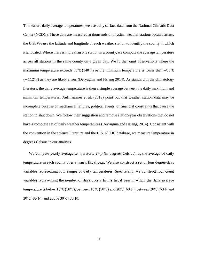
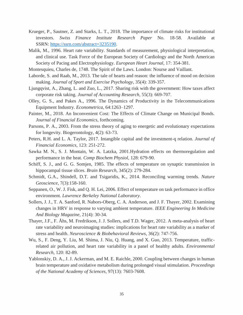
Figure 1 plots the average temperature each year between 1969 and 2015 across all U.S counties

where plants in our sample are located. While plant-level data begin in 1990, we extend the sample

period in these graphs to 1969, which exhibit a visible trend of rising temperature over time. The

first graph shows that the country’s average temperature rises every year. In 1969, the average

temperature in the U.S. is about 11.7℃ (53.06℉). By the end of our sample period in 2015, the

average temperature has risen to 12.6℃ (54.68℉). Consistently, we see a rise in both the average

high and low temperatures across the nation. Over a shorter, more recent sample period 1990-2015,

the rising trend is less visible.

Figure 1 also exhibits a feature that is preferable for our empirical analysis: there is a significant

year-on-year variation in the average temperature. This variation indicates that even when a plant

chooses to locate in a county of predominantly warm climate, the local average temperature can

be colder in one year than another and potentially affect the mood and cognitive ability of workers

as scientific studies suggest.

< Insert Figure1 around here >

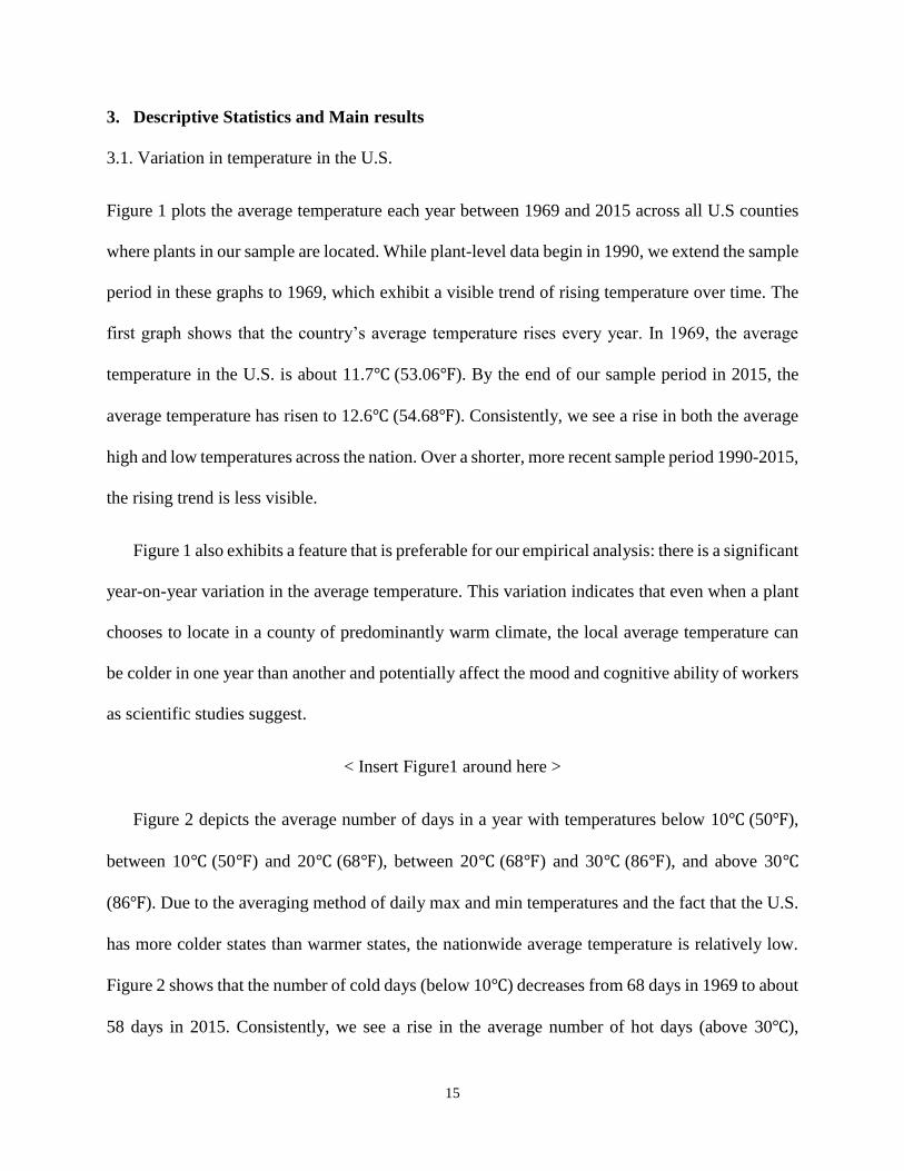
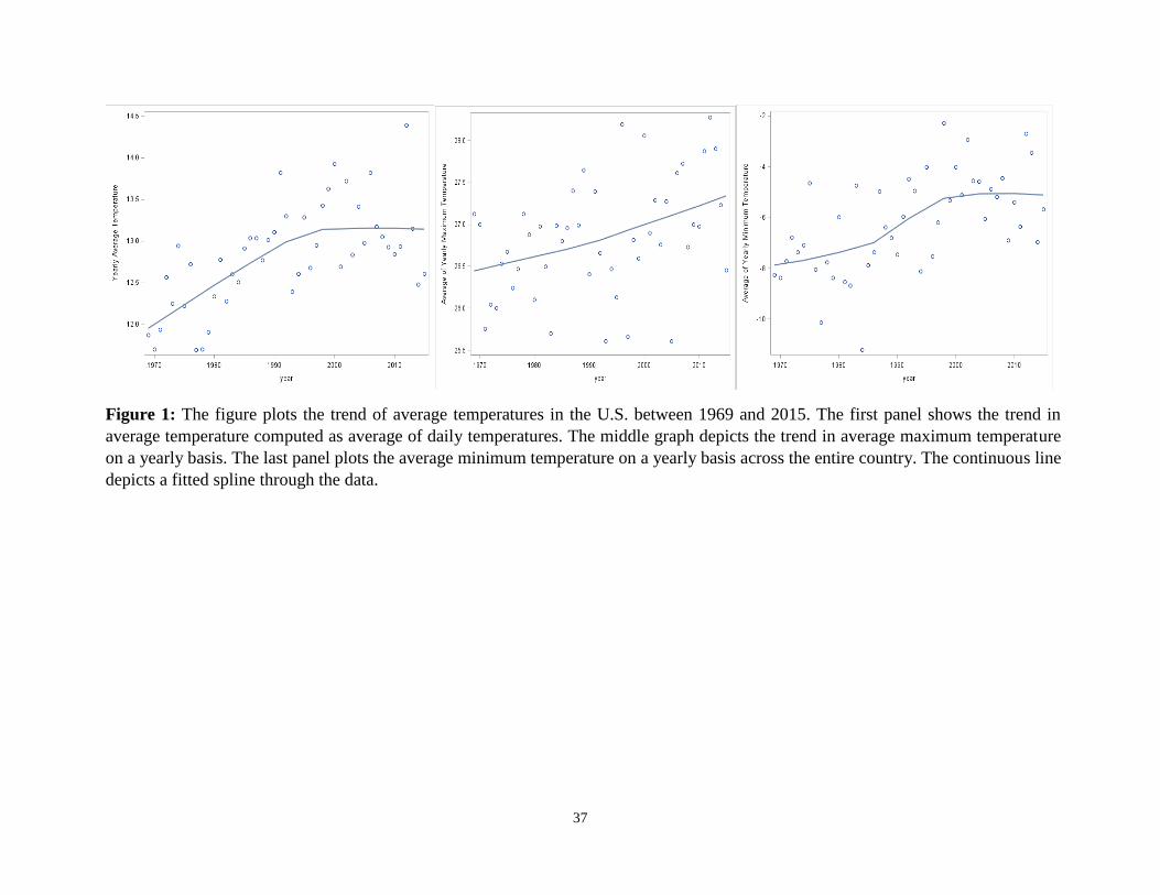
Figure 2 depicts the average number of days in a year with temperatures below 10℃ (50℉),

between 10℃ (50℉) and 20℃ (68℉), between 20℃ (68℉) and 30℃ (86℉), and above 30℃

(86℉). Due to the averaging method of daily max and min temperatures and the fact that the U.S.

has more colder states than warmer states, the nationwide average temperature is relatively low.

Figure 2 shows that the number of cold days (below 10℃) decreases from 68 days in 1969 to about

58 days in 2015. Consistently, we see a rise in the average number of hot days (above 30℃),

16

ranging from about one day in 1969 to about two days in 2015. Consistent with Figure 1, there are

also significant year-on-year variations in each of the temperature-day variables.

< Insert Figure 2 around here >

3.2. Univariate relation between temperature and plant-level productivity and summary statistics

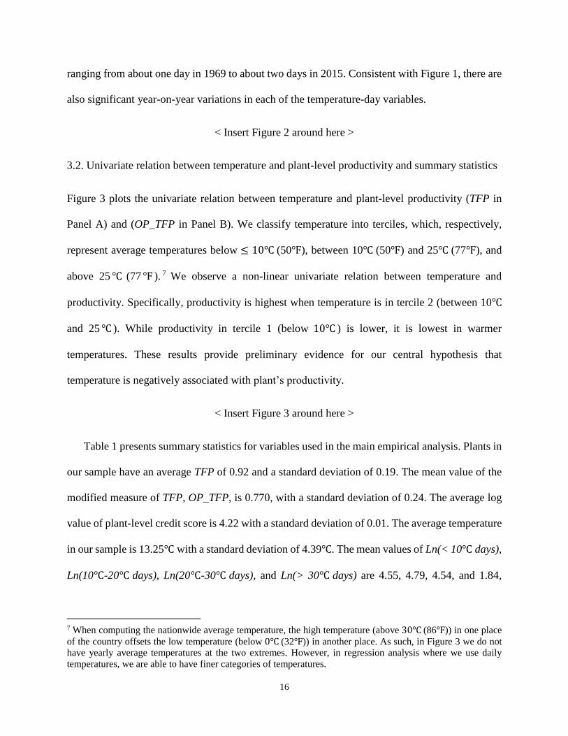
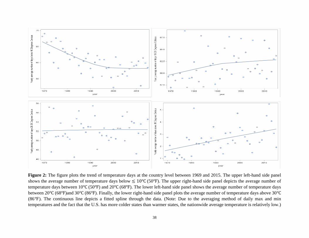
Figure 3 plots the univariate relation between temperature and plant-level productivity (TFP in

Panel A) and (OP_TFP in Panel B). We classify temperature into terciles, which, respectively,

represent average temperatures below ≤ 10℃ (50℉), between 10℃ (50℉) and 25℃ (77℉), and

above 25 ℃ (77 ℉ ). 7 We observe a non-linear univariate relation between temperature and

productivity. Specifically, productivity is highest when temperature is in tercile 2 (between 10℃

and 25 ℃ ). While productivity in tercile 1 (below 10℃ ) is lower, it is lowest in warmer

temperatures. These results provide preliminary evidence for our central hypothesis that

temperature is negatively associated with plant’s productivity.

< Insert Figure 3 around here >

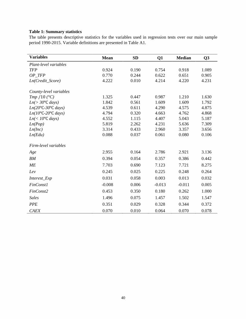
Table 1 presents summary statistics for variables used in the main empirical analysis. Plants in

our sample have an average TFP of 0.92 and a standard deviation of 0.19. The mean value of the

modified measure of TFP, OP_TFP, is 0.770, with a standard deviation of 0.24. The average log

value of plant-level credit score is 4.22 with a standard deviation of 0.01. The average temperature

in our sample is 13.25℃ with a standard deviation of 4.39℃. The mean values of Ln(< 10℃ days),

Ln(10℃-20℃ days), Ln(20℃-30℃ days), and Ln(> 30℃ days) are 4.55, 4.79, 4.54, and 1.84,

7 When computing the nationwide average temperature, the high temperature (above 30℃ (86℉)) in one place

of the country offsets the low temperature (below 0℃ (32℉)) in another place. As such, in Figure 3 we do not

have yearly average temperatures at the two extremes. However, in regression analysis where we use daily

temperatures, we are able to have finer categories of temperatures.

17

respectively. Appendix Table A3 provides state-by-state summary statistics of average

temperatures. The top 5 coldest states are North Dakota, Montana, Wyoming, Vermont, and Maine

with the average temperatures ranging from 4℃ (39℉) to 6℃ (43℉). The top 5 warmest states are

Florida, Arizona, Louisiana, Texas, and Mississippi with the average temperatures ranging from

18℃ (64℉) to 23℃ (73℉).

The statistics of other control variables indicate that, on average, firms have the log value of

age (Age) of 2.95, a log value of BM of 0.39, a log value of firm size (ME) of 7.70, leverage (LEV)

of 0.25, a delay investment score (FinConst1) of −0.01, interest expense ratio of 0.02, log value

of sales of 1.23, asset tangibility (PPE) of 0.31, and capital expenditure (CAEX) of 0.07.

Approximately 45% of our plant-year observations have missing Hoberg and Maksimovic’s (2015)

delay investment score. Thus, to be conservative, in addition to these text-based measures of

financial constraints, we also control for interest expense ratio and plant-level credit scores in all

regressions.

Appendix Table A2 presents pairwise correlations between variables used in our study.

Temperature is negatively correlated with plant’s TFP and OP_TFP. These productivity measures

are also negatively correlated with Ln(>30℃ days), which is the number of days above 30℃ (86℉)

in a given year.

3.3. Multivariate analysis

We start our main empirical analysis by investigating the relation between temperature and plant-

level productivity. Our null hypothesis is that there is no relation between temperature and

performance. This null hypothesis is based on the premise that with the advances of modern

18

technologies such as fully air-conditioned offices, possibly coupled with human body’s adjustment

to the surrounding environment, workers are no longer affected by presumably random variations

in daily temperatures. The alternative hypothesis is derived from that the biomedical literature,

which suggests that the cognitive and physical abilities of workers still do not function well in the

warmer temperature. These effects, in turn, decrease workers’ productivity.

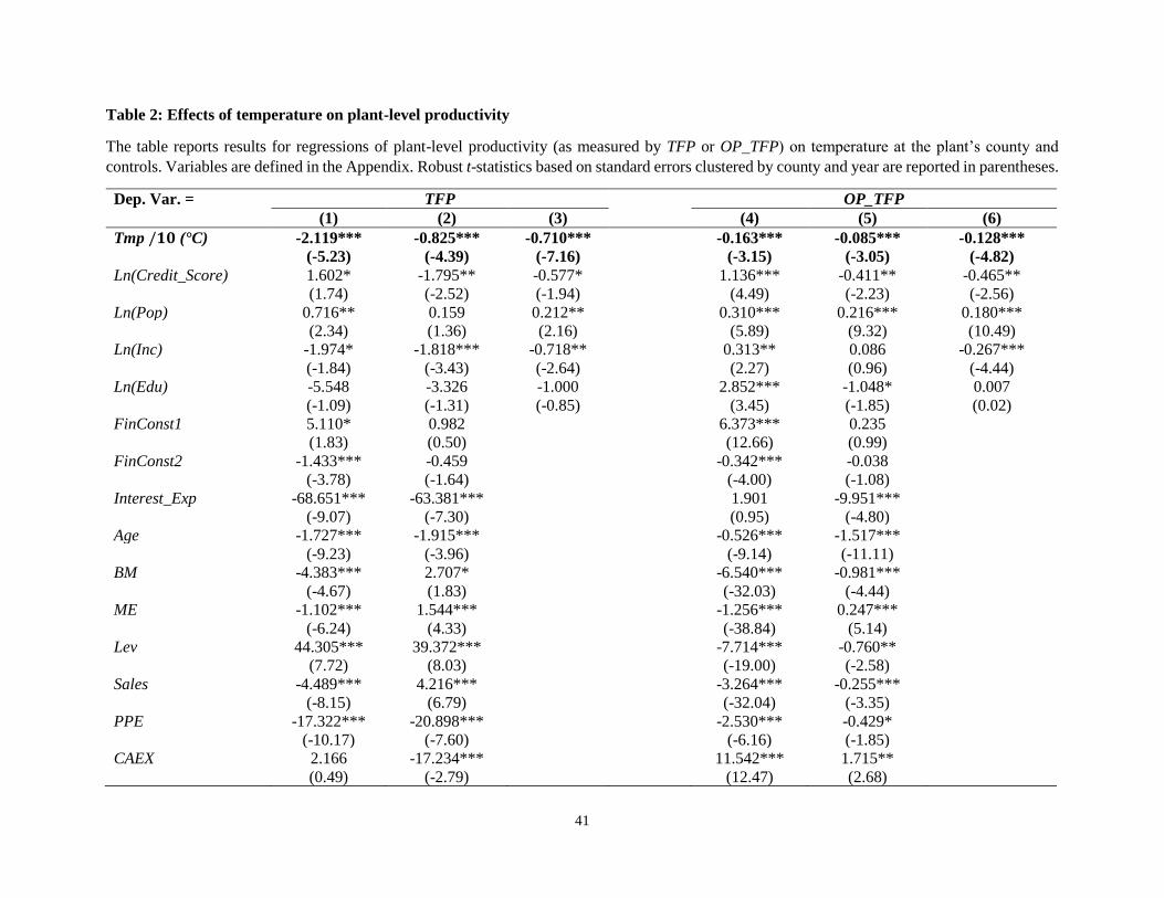
Table 2 reports results of different regression models of plant-level TFP (Models (1)-(3)) or

OP_TFP (Models (4)-(6)) on temperature and controls. For each alternate measure of plant-level

performance, we subsequently control for industry, county, and year fixed effects (Model (1) and

Model (4)), firm, year, and county fixed effects (Model (2) and Model (5)), and county, firm ×

year fixed effects (Model (3) and Model (6)). Since temperature is measured at the county level,

we report robust t-statistics clustered by county and year to correct for potential serial correlation.

To reduce the number of decimals in the coefficient estimate, we scale the temperature variable by

10.

In all models, the coefficient on temperature is negative and statistically significant at the 1

percent level, suggesting that plant’s productivity is lower when local temperature is higher. The

effect is also economically significant. For example, the coefficient on temperature of −0.825 in

Model (2) indicates that when yearly local temperature increases by 1°𝐶 (which is less than one

standard deviation of 4.4°𝐶), plant’s TFP decreases by 8.9% compared to the sample mean.8 For

another perspective, this marginal effect means that the TFP ranking of the affected plant drops

from the 75𝑡ℎ percentile of 1.089 (reported in Table 1) to roughly the 60𝑡ℎ percentile of 1.007 (not

tabulated) in the cross-section of plants in the U.S. Similarly, the coefficient on temperature in

8 Using the summary statistics in Table 1, the economic impact of temperature on TFP is equal to

(−0.825

10× 1℃)/0.924, where 0.924 is the sample mean of TFP.

19

Model (6) shows that a 1°𝐶 increase in yearly temperature results in a reduction in plant-level

OP_TFP by 1.7% relative to the sample mean.

< Insert Table 2 around here >

4. Additional Analysis

4.1. Effects of temperature on plants relocating to states with warmer temperature and lower tax

rates

Previous section documents a strong and robust effect of temperature on plant-level productivity.

While fluctuations in temperature are random and exogenous to firms’ characteristics, endogeneity

issues are possible because the choice of a plant’s location may not be random: firms may choose

to base their plants in counties where their employees are most comfortable with the climate of

those counties and hence become more productive. To mitigate these concerns, we take the

advantage of plant relocation events that are likely due to state-level tax policy changes. We

identify a sample of plants that moved from a colder, higher-tax county to a warmer, lower-tax

county within two years after a tax-rate reduction law in the destination state was passed. We

contend that these plant relocations are possibly motivated by lower corporate tax rates, since

Giroud and Rauh (2018) find strong causal evidence that a decrease in state-level corporate tax

rate leads to more new plants in the state.

We obtain information on state-level tax policy changes from Heider and Ljungqvist (2015).

A destination county is considered warmer than the origin county if its average temperature in the

past five years is one degree Celsius higher than that of the origin county. Since temperature in the

destination county varies on a yearly basis and it may happen to be colder in the relocation year,

we require that the average temperature in the destination county in the event year be at least 0.5

20

degree Celsius higher than its own temperature in the prior year. We create a Post dummy variable

that takes a value of one to indicate the two years after the relocation of a treatment plant. We

employ two sets of control plants. The first control sample contains all other plants that do not

experience such relocation events. For the second control sample, we use plants that relocate to a

colder, lower-tax state.

Examining these relocation events yields at least three advantages. First, firms presumably

relocate their plants for economic reasons such as lower corporate tax rates (Giroud and Rauh

2018)), and variation in temperature is likely to be exogenous to this choice. Second, to the extent

that firms choose to relocate their plants to a lower tax county with warmer temperature, we should

no longer find a negative effect of temperature on productivity of these relocated plants because

these plants may have already considered the negative impacts of warmer temperature and adopted

measures to prevent potential negative impacts of hotter temperature. Thus, these events make our

tests more conservative and bias against finding an effect of temperature on productivity. Third,

relocations events are “staggered” at the plant level and affect plant’s productivity at different

points in time. As argued by Roberts and Whited (2011), Edmans, Jayaraman, and Schneemeier

(2017) and others, staggered events provide researchers with a setting similar to a difference-in-

difference (DiD) analysis that avoids the common challenge faced by studies using a single

systematic shock, which affects all plants at the same time. At the same time, there are a number

of plants that enjoy the benefit of lower corporate tax rates in counties with a colder climate. These

plants are included in the potential control group in our DiD analysis, thereby helping to filter out

common temporal trends between treatment and control plants (Guo and Masulis 2015).

Table 3 Panel A reports the DiD analysis using all non-event plant-years as control group.

Model (1) and (2) report results for the regression of TFP, while Model (3) and Model (4) present

21

results for the regression of OP_TFP. The coefficient on Post in Model (1) where firm, county and

year fixed effects are included, is −0.211 with an associated t-statistic of −2.80 , which is

significant at the 1 percent level. This coefficient estimate indicates that treatment plants

experience a reduction in TFP by 21% (or 23% relative to the sample mean) after relocating to a

hotter, lower-tax county. Model (2) shows similar results when we include county and firm × year

fixed effects. Consistently, Model (3) uses OP_TFP as the dependent variable and shows that the

coefficient on Post is −0.142 (t-statistic of −2.36 ). In terms of economic magnitude, this

reduction in performance of treatment plants represents 18% of the unconditional mean of

OP_TFP.


A potential concern regarding the DiD analysis is that the difference between treatment and

control groups may exist prior to the real event year. We formally test the parallel trend assumption

by employing “pseudo-events” that happen before the actual event. Specifically, we create a

dummy variable Pseudo_Event, which takes a value of one for treatment firms in the two years

surrounding the actual relocation event.9 We also control for Post, which is the actual event

dummy. If the parallel trend assumption is rejected, we should observe a significant coefficient on

Pseudo_Event. Table 3 Panel B shows that the coefficient on Pre_Event is insignificant for both

regressions of TFP and OP_TFP, while the coefficient on the actual Post event dummy remains

statistically significant. This result re-assures the validity of our relocation events.

9 In unreported analysis, we use two years before the actual relocation event as Pseudo_Event variable and our

results do not qualitatively change.

22

4.2.Temperature days and plant-level performance

In this section, we examine whether plant’s performance is lower in hotter years. We construct

four count variables representing the number of days over a firm’s fiscal year during which the

daily average temperature is below 10℃ (50℉), between 10℃ (50℉) and 20℃ (68℉), between

20℃ (68℉)and 30℃ (86℉), and above 30℃ (86℉). Table 4 reports estimation results for

regressions of plant-level TFP (Model (1) and Model (2)) and OP_TFP (Model (3) and Model (4))

on these four temperature days variables and controls. In Models (1) and (2), we observe an

inverted U-shaped relation between temperature days and TFP. The coefficient on Ln(< 10℃

days) is negative −0.048, while the coefficient on Ln(10℃-20℃ days) is positive and statistically

significant at the 1% level. As there are more warmer days in a year, TFP is lower with the

coefficients on Ln(20 ℃ -30 ℃ days) and Ln(> 30 ℃ days) being negative and statistically

significant at the 1% level.

The effect of cold temperature on TFP, however, is not robust in Models (3) and (4), where

the dependent variable is OP_TFP, which allows plants to change the level of inputs as

productivity changes. The coefficient on Ln(< 10℃ days) in the last two columns is insignificant

even at the 10% level, whereas the coefficient on Ln(> 30 ℃ days) remains negative and

statistically significant. Ln(10℃-20℃ days) has a positive effect on OP_TFP with the coefficient

being positive and significant at the 1% level, suggesting that productivity is highest in this

temperature range.


These results indicate that there is an inverted U-shaped relation between temperature and

plant-level productivity. However, the effect of extremely hot temperature is stronger and more

robust than that of cold temperature. Plant-level productivity is highest when the ambient

23

temperature is between 10℃ and 20℃. These results are consistent with scientific findings that hot

temperature has a more significant impact on workers’ health and productivity than cold

temperature.10

4.3. Customer demand versus supplier productivity

A potential confounding effect is that plant’s performance may be lower due to lower demand of

their products rather than productivity of workers. To rule out this alternative explanation, one

would ideally need to observe the location of each customer of each plant. Unfortunately, to the

best of our knowledge, such data are not publicly available. We thus follow Agrawal and Matsa

(2013) and employ data from the U.S. Commodity Flow Survey, which is conducted by the U.S.

Bureau of the Census and surveys plants across the U.S. on the total revenues of goods shipped to

intrastate and interstate customers. Using this dataset, we examine a sample of plants, whose 95%

of sales revenues come from out-of-state customers.

We regress plant-level TFP and Tobin’s Q on its home county’s temperature for this sample

of plants, whose sales are mainly generated out of their home states. Table 5 reports regression

results. Model (1) and Model (2) present the regression of TFP, while Model (3) and Model (4)

report regression results for OP_TFP. In all the four models, the coefficient on local temperature

is negative and statistically significant at the conventional level. These results suggest that even

for plants that make most of their revenues from non-local customers are still affected by the local

temperature of their counties.


10 Scientific research also shows that human body functions best when the ambient temperature is around 21℃

(70°F) (https://www.scientificamerican.com/article/why-people-feel-hot/)

https://www.scientificamerican.com/article/why-people-feel-hot/

24

4.4. Agriculture and outdoor industries

Our hypothesis is that temperature affects plant’s performance through lower workers’

productivity. This hypothesis builds on the health science literature that ambient temperature

affects both indoor and outdoor workers. Nevertheless, we expect that the effect should be stronger

for plants in industries that are more exposed to temperature such as agriculture and outdoor

industries.

Using the SIC code of each plant from the NETS database, we construct a dummy variable,

Agriculture, which indicates plants in the agriculture industry based on Fama and French’s

industry classifications (those with SIC codes 0100-0799). We also create an indicator variable,

Outdoor, which takes a value of 1 for establishments of outdoor industries such as construction

and transportation (those with SIC codes 1500-2459 and 4000-4789). We then regress plant-level

TFP and OP_TFP on temperature, its interaction with each of these indicator variables, and

controls. Since the SIC code does not change frequently for each firm, we cannot employ firm

fixed or industry fixed effects in these regressions. Thus, we control for year and county fixed

effects in this analysis.


Table 6 reports regression results. Models (1) and (2) use TFP is the dependent variable, while

Models (3) and (4) employ OP_TFP as the dependent variable. Model (1) shows that the

coefficient on the interaction term between temperature and Agriculture is negative and

statistically significant at the 1% level. In Model (2), the coefficient on the interaction term

between temperature and Outdoor is also negative and significant at the 1% level. Model (3) and

Model (4) show consistent results for OP_TFP. In all models, the coefficient on temperature

25

remains significant and negative. These results indicate that while temperature affects productivity

of an average firm across all industries, the effect is larger for agriculture and outdoor industries.

4.5. How does warmer temperature affect productivity? Innovation channel

If temperature affects plant’s productivity via the cognitive ability of workers, then corporate

innovation and patent quality, which are heavily dependent on creativity and productivity of

inventors, would also be lower in regions with warmer temperature. We obtain innovation data

from Kogan et al. (2017) for the period 1990-2010. Following prior studies in innovation, we

assume that it takes, on average, about two years from the development stage to the application

date of the patent.

To measure innovation at each plant, we identify the location of each inventor of a patent in

Kogan et al.’s (2017) database using inventor-level information from the U.S. Patent Inventor

Database. For each patent, the U.S. Patent Inventor Database provides a unique identifier of an

inventor, location of the inventor, patent ID, and the assignee (i.e., the firm that owns the patent).

We match this information with patent data of Kogan et al. (2017) together with the plant’s location

from NETS to obtain the innovation level at each plant.

We estimate the regression of the natural logarithm of number of patents and patent citations

on local county’s temperature, controlling for firm, year, and county fixed effects or firm-by-year

and county fixed effects. Table 7 reports regression results. In Models (1) and (2), where the

dependent variable is the natural logarithm of number of patents at each plant, Ln(Patents), the

coefficient on temperature is −0.627 and −0.665 with an associated t-statistic of −3.36 and

−3.21, which are statistically significant at the 1 percent level. The magnitude of these coefficients

26

is also economically significant. For example, the coefficient estimate on temperature in Model (1)

suggests that an increase in yearly temperature by 1℃ leads to a reduction in Ln(Patents) by 2.6%

relative to the sample mean.11 Model (3) and Model (4) regress the natural logarithm of patent

citations on temperature and controls. We observe that the coefficient on temperature remains

negative and statistically significant at the 1 percent level. Consistent with the biomedical

prediction, these results suggest that warmer temperature impacts productivity of inventors,

causing innovation at the plant to be lower.


In Table 7 Panel B, we examine whether our results are driven by the state of California, where

many innovative firms are located. We remove establishments in California and re-estimate the

innovation regression. The coefficient on temperature remains negative and significant, suggesting

that our results are not driven by these California-based firms.

Since inventors are highly skilled employees, they are relatively able to migrate out of hotter

counties if warm temperature impairs their cognitive ability and creativity. Such brain drain can

cause plants in these counties to lose talents in the medium to long run, and as a result, innovation

of these firms to be lower. To empirically test this prediction, we employ inventor-level data from

the U.S. Patent Inventor Database and compute the number of inventors in each county in each

year. Since inventors do not necessarily migrate out of a county immediately after temperature in

a given year is warmer, we focus on examining the effect of medium- to long-term average

temperature on the medium- to long-term average number of inventors (net of inflows and

outflows).

11 This is computed as (−

0.627

10× 1℃)/2.39, where 2.39 is the sample average of Ln(Patents).

27

Results are reported in Table 7 Panel C. Model (1) regresses the natural logarithm of three-

year average number of inventors in a county on three-year average temperature. Model (2)

regresses the natural logarithm of five-year average number of inventors in a county on the five-

year average temperature, while Model (3) uses ten-year averages. In all models, the coefficient

on average temperature is negative and statistically significant at the 1 percent level, suggesting

that counties lose more talents as medium- and long-term average temperatures are higher. The

effect is also economically significant. For example, the coefficient on temperature in Model (1)

indicates that when the three-year average temperature increases by 1℃, the talent pool in the

county decreases by 1%, representing 0.23% of the sample average, which is equivalent to a net

outflow of 595 inventors out of the county.12

Our last test of the innovation channel examines whether the negative impact of warmer

temperature on innovative activities would result in lower the overall productivity and

performance of a firm. To do so, we first estimate a plant’s overall productivity sensitivity to

innovation. Specifically, we estimate a 10-year rolling regression of a plant’s TFP or OP_TFP on

the natural logarithm of number of patents (Ln(Patents)). The annual coefficient on Ln(Patents),

denoted as 𝛽𝑡𝑚𝑝𝑖𝑛𝑛𝑜, represents a plant’s performance sensitivity to innovation. In the second stage,

we regress a plant’s TFP or OP_TFP on temperature, 𝛽𝑡𝑚𝑝𝑖𝑛𝑛𝑜, and the interaction between these two

variables, and controls. Table 7 Panel D reports regression results. The coefficient on the

interaction term, 𝛽𝑡𝑚𝑝𝑖𝑛𝑛𝑜 × 𝑇𝑚𝑝 is negative and significant at the 1 percent level in all the four

models. This suggests that the effect of temperature on a plant’s productivity is larger if it is more

dependent on innovation outputs of inventors.

12 0.23% =

0.182/10

7.85× 100, where 7.85 is the mean of Ln(3-year average of number of inventors in a county).

28

4.6. How does rising temperature affect productivity? Mental health channel

The science and health economics literature documents that warmer temperature can cause human

conflicts, bad mood, and suicide rates (Hsiang, Burke, and Miguel 2013; Burke et al. 2018). To

the extent that suicide rate in a county is sensitive to warmer temperature in a given year, we expect

that productivity of workers in the county is also lower in the year. To test this conjecture, we

obtain suicide rates in each county from the Center for Disease Control and Prevention for the

period 1999-2014.13 For each county, we estimate ten-year rolling regressions of suicide rate on

temperature and retain the time-series of the coefficient, denoted 𝛽𝑡𝑚𝑝𝑠𝑢𝑖𝑐𝑖𝑑𝑒, which is the suicide rate

sensitivity to temperature of each county. In the second stage, we regress a plant’s TFP or OP_TFP

on temperature, 𝛽𝑡𝑚𝑝𝑠𝑢𝑖𝑐𝑖𝑑𝑒, and the interaction between these two variables, controls, and firm, year,

county fixed effects as well as firm-by-year and county fixed effects.

Table 8 Panel A reports the regression results. Model (1) and Model (2) use plant-level TFP

as the dependent variable, while the dependent variable in Model (3) and Model (4) is plant-level

OP_TFP. The coefficient on the interaction term between temperature and 𝛽𝑡𝑚𝑝𝑠𝑢𝑖𝑐𝑖𝑑𝑒 is negative and

statistically significant at the 1 percent level in all regressions. These results suggest that

productivity is significantly lower for plants located in counties, where the residents’ mental health

is more sensitive to warmer temperature. These results provide further supporting evidence for the

notion that temperature affects cognitive ability of workers in the county.


4.7. How does rising temperature affect productivity? Physical health channel

13 The data are obtained from https://wonder.cdc.gov/wonder/help/ucd.html, which are available since 1999.

https://wonder.cdc.gov/wonder/help/ucd.html

29

Warm temperatures can also cause physical health issues and dehydration for employees located

in the warm county. To examine whether plant’s productivity is lower in counties where residents

are more likely to be hospitalized due to injuries, we collect hospital admissions data in each

county in California from the Center for California health and human services open data portal

website for the period 2010-2014. 14 To derive a measure of physical health sensitivity to

temperature, we estimate a regression of county’s average number of days admitted to hospital per

patient on temperature in that county using all data between 2010 and 2014 for each county in

California. The physical health sensitivity to temperature of each county is the coefficient on

temperature, denoted 𝛽𝑡𝑚𝑝ℎ𝑜𝑠𝑝𝑖𝑡𝑎𝑙

, obtained from these regressions. In the second stage, we regress a

plant’s TFP or OP_TFP on temperature, 𝛽𝑡𝑚𝑝ℎ𝑜𝑠𝑝𝑖𝑡𝑎𝑙

, and the interaction between these two variables,

and controls.

We report results in Table 8 Panel B. In all models, the coefficient on the interaction term

between temperature and 𝛽𝑡𝑚𝑝ℎ𝑜𝑠𝑝𝑖𝑡𝑎𝑙

is negative and statistically significant at the conventional level.

These results suggest that productivity is significantly lower for plants located in counties where

residents’ physical health is more sensitive to hotter temperature.

4.8. Firm-level analysis: Tobin’s Q

In this subsection, we examine whether our results still hold at the firm level. Since a firm may

have plants in different counties, we follow Heidi and Ljungqvist (2015) and Ljungqvist, Zhang,

14 Admissions data are publicly available for hospitals in California only. The data are obtained from

https://data.chhs.ca.gov/dataset/patient-discharge-data-by-admission-type, which are available from 2010 to

2014. We manually collect information on the location of each hospital from Google searches and hospital

websites.

30

and Zhang (2017) and compute the weighted temperature in a firm’s nexus states in a fiscal year

as follows:

𝑊𝑒𝑖𝑔ℎ𝑡𝑒𝑑 𝑇𝑚𝑝 = (0.5 ×𝑠𝑎𝑙𝑒𝑠𝑝,𝑖

𝑡𝑜𝑡𝑎𝑙 𝑠𝑎𝑙𝑒𝑠𝑖+ 0.5 ×

𝑒𝑚𝑝𝑙𝑜𝑦𝑒𝑒𝑠𝑝,𝑖

𝑡𝑜𝑡𝑎𝑙 𝑒𝑚𝑝𝑙𝑜𝑦𝑒𝑒𝑠𝑖) 𝑇𝑚𝑝𝑝

where 𝑠𝑎𝑙𝑒𝑠𝑝,𝑖 and 𝑒𝑚𝑝𝑙𝑜𝑦𝑒𝑒𝑠𝑝,𝑖 are sales and number of employees at plant p of firm i;

𝑡𝑜𝑡𝑎𝑙 𝑠𝑎𝑙𝑒𝑠𝑖 and 𝑡𝑜𝑡𝑎𝑙 𝑒𝑚𝑝𝑙𝑜𝑦𝑒𝑒𝑠𝑖 are total sales and employees across all plants of the firm; and

𝑇𝑚𝑝𝑝 is the average yearly temperature in the county of plant p.

We repeat the main regression at the firm level and report estimation results in Table 9. Model

(1) and Model (2) examine the effect of weighted temperature on firm-level Tobin’s Q, while

Model (3) and Model (4) regress Tobin’s Q on weighted temperature-days variables. We

alternately control for industry, county, and year fixed effects as well as firm, year, and county

fixed effects. Models (1) and (2) show that the coefficient on weighted temperature is negative and

statistically significant at the 1 percent level. Consistent with the plan-level results, these findings

suggest that firm performance is lower when its plants are affected by warmer temperature. In

Models (3) and (4), we can see that the coefficient on weighted Ln(> 30℃ days) is negative and

statistically significant at the 1 percent level. While the coefficients on other temperature days are

also significant in Model (3) with industry, county and year fixed effects, they become

insignificant when we control for firm, county, and year fixed effects. These results show that the

effect of hot temperature on firm performance is strong and robust to different research designs.


4.9. Placebo analysis using temperature on weekend

In this subsection, we test whether the relation between temperature and plant-level productivity

is a spurious result. We do so by taking advantage of the fact that a majority of economic activities

31

occur during weekdays, rather than weekends (Deryugina and Hsiang, 2013). If our results are

spurious, we expect that the effect of weekend temperature to be significant. Table 10 reports

estimation results. Across all regression models, the coefficient on weekend temperature is

statistically insignificant even at the 10% level and the estimate is also economically small. These

results suggest that plant-level productivity is not affected by temperature on weekends and that

the baseline relation documented in our study is not a spurious result.


4.10. Controlling for other weather variables

Our next sensitivity analysis addresses a concern that temperature could be correlated with other

weather variables, such as precipitation, evaporation, sunshine time, and wind speed. We thus

control for these dimensions of weather, which are obtained from the NCDC database, and report

results in Table 11. In general, the effects of temperature on plant-level TFP (Model (1) and Model

(2)), OP_TFP (Model (3) and Model (4)), remain robust after controlling for these additional

weather-related variables. Among these other weather variables, only evaporation shows a

marginally significant effect on plant-level TFP in one model specification. These results suggest

that the effect of temperature is not confounded by other weather events.


4.11. Effects of long-run temperature on long-run productivity

Our final avenue of analysis examines whether the effect of yearly temperature translates into a

long-run effect. This has implications for the cost of climate change, which refers to the long-run

rising temperature. Since the impact of long-term climate trend is an aggregation of short-term

effects of temperature changes over time (Schmidt, Shindell, and Tsigaridis 2014), we expect that

rising long-term temperature should also have a negative impact on plant-level productivity.

32

To test this implication, we compute moving averages of temperature, TFP and OP_TFP over

the windows of three, five, and ten years. Table 12 reports results for the regression of moving-

average TFP and OP_TFP on the corresponding moving average temperature and controls. Across

all models, the coefficient on the long-term temperature is negative and statistically significant at

the 1 percent level. These results suggest that the long-term productivity of plants is lower as long-

term temperature rises.


5. Conclusion

Employing plant-level data for U.S. firms and data on county-level temperature, this paper

provides one of the first U.S. evidence on whether, and how, temperature affects business

productivity and firm performance. Findings of our paper therefore have direct implications for

managers and policymakers. Our study also extends the scope of an emerging literature on climate

finance, which focuses on investigating the micro-level effect of climate risk and the efficiency of

capital markets in pricing the impact of climate change.

We find strong evidence that rising temperature negatively affects plant-level productivity

measured by total factor productivity and firm-level performance measured by Tobin’s Q. The

effect remains robust to examining a sample of plants that choose to relocate from a colder county

to a hotter county, presumably for tax-motivated reasons. This result suggests that self-selection

of plants to be based in warmer counties cannot fully explain our findings.

We explore the channels through which rising temperature impedes productivity. Consistent

with the science literature, which suggests that warmer temperature impairs the cognitive ability

and productivity of employees, we find that the quality and quantity of inventors’ innovation are

lower. Moreover, the effect is stronger for plants, whose overall performance is more dependent

33

on productivity of inventors. We also find that plant-level productivity is lower in counties where

residents’ mental health and physical health are more sensitive to warm temperature. Overall, our

study contributes to the literature examining the cost of warming temperature. Findings in our

study also fit into the existing climate finance literature as they serve as a potential mechanism for

why investors should be concerned about the consequences on rising temperature in capital

markets.

References

Acharya, V., Baghai, R., Subramanian, K., 2014. Wrongful discharge laws and innovation. Review

of Financial Studies, 27: 301–47.

Agrawal, A.K. and Matsa, D.A., 2013. Labor unemployment risk and corporate financing

decisions. Journal of Financial Economics, 108(2): 449-470.

Auffhammer, M., S. Hsiang, W. Schlenker, and A. Sobel, 2013. Using weather data and climate

model output in economic analyses of climate change. Review of Environmental Economics

and Policy 7 (2):181-198.

Ayoko, O. B., Callan, V. J. and C. E. Härtel, 2003. Workplace conflict, bullying, and

counterproductive behaviors. The International Journal of Organizational Analysis, 11(4),

pp.283-301.

Baldauf, M., Garlappi, L., and Yannelis, C., 2018. Does climate change affect real estate prices?

Only if you believe in it. Available at SSRN: https://ssrn.com/abstract=3240200.

Bansal, R., Kiku, D., Ochoa, M., 2016. Price of long-run temperature shifts in capital markets.

Tech. rep. National Bureau of Economic Research.

Basu, S., John G. F., and Miles S. K., 2006. Are technology improvements contractionary?.

American Economic Review, 96: 1418–1448.

Bernstein, A., Gustafson, M., Lewis, R., 2017. Disaster on the horizon: The price effect of sea

level rise. Working Paper.

Burke, M., S. M. Hsiang, and E. Miguel, 2015. Global non-linear effect of temperature on

economic production. Nature, 527(7577): 235-239.

Burke, M., González, F., Baylis, P., Heft-Neal, S., Baysan, C., Basu, S. and Hsiang, S., 2018.

Higher temperatures increase suicide rates in the United States and Mexico. Nature climate

change, 8(8):723-729.

Chang, X., Fu, K., Low, A., Zhang, W., 2015. Non-executive employee stock options and

corporate innovation. Journal of Financial Economics, 115: 168–188.

https://ssrn.com/abstract=3240200

34

Choi, D., Gao, Z., and Jiang, W., 2019. Attention to Global Warming. Review of Financial Studies

forthcoming.

Davis, M.A. (2009). Understanding the relationship between mood and creativity: A meta-analysis.

Organizational Behavior and Human Decision Processes, 108: 25-38.

Dell, M., Jones, B.F. and Olken, B.A., 2012. Temperature shocks and economic growth: Evidence

from the last half century. American Economic Journal: Macroeconomics, 4(3): 66-95.

Deryugina, T. and S. M. Hsiang, 2014. Does the environment still matter? Daily temperature and

income in the United States. National Bureau of Economic Research (No. 20750).

Deschênes, O. and M. Greenstone. 2007. The economic impacts of climate change: Evidence from

agricultural output and random fluctuations in weather. American Economic Review, 97 (1):

354-385

Faccio, M. and HSU, H.C., 2017. Politically connected private equity and employment. The

Journal of Finance, 72(2): 539-574.

Federspiel C. C., W. J. Fisk, P. N. Price, G. Liu, D. Faulkner, D. L. Dibartolemeo, D. P. Sullivan,

M. Lahiff, 2004. Worker performance and ventilation in a call center: analyses of work

performance data for registered nurses. Indoor Air Journal, 14. Supplement 8: 41-50.

Gates, W. E., 1967. The Spread of IBN Khaldun’s Ideas on Climate and Culture. Journal of the

History of Ideas 28 (3): 415–22.

Gormley, T.A. and Matsa, D.A., 2014. Common Errors: How to (and Not to) Control for

Unobserved Heterogeneity. Review of Finial Studies, (27): 646-51.

Guo, L., and Masulis, R.W., 2015. Board structure and monitoring: New evidence from CEO

turnovers. Review of Financial Studies (28): 2770-2811.

Heider, F. and Ljungqvist, A., 2015. As certain as debt and taxes: Estimating the tax sensitivity of

leverage from state tax changes. Journal of Financial Economics, 118(3): 684-712.

Hoberg, G. and Maksimovic, V., 2014. Redefining financial constraints: A text-based analysis.

Review of Financial Studies, 28(5): 1312-1352.

Hsiang, S.M., 2010. Temperatures and cyclones strongly associated with economic production in

the Caribbean and Central America. Proceedings of the National Academy of sciences, 107:

15367-15372.

Hsiang, S.M. and M. Burke, 2014. Climate, conflict, and social stability: what does the evidence

say?. Climatic Change, 123(1): 39-55.

Hong, H.G., F.W. Li., and J. Xu, 2018. Climate risks and market efficiecy. Journal of

Econometrics, 208(1): 265-81.

Kilbourne, E.M., 1997: Heatwaves. In: The Public Health Consequences of Disasters [Noji, E.

(ed.)]. Oxford University Press, Oxford, United Kingdom and New York, NY, USA, pp. 51–

61.

Kilbourne, E. M. 1997. Heat waves and hot environments. The public health consequences of

disasters, 245-269.

Kogan, L., Papanikolaou, D., Seru, A. and Stoffman, N., 2017. Technological innovation, resource

allocation, and growth. The Quarterly Journal of Economics, 132(2): 665-712.

35

Krueger, P., Sautner, Z. and Starks, L. T., 2018. The importance of climate risks for institutional

investors. Swiss Finance Institute Research Paper No. 18-58. Available at

SSRN: https://ssrn.com/abstract=3235190.

Malik, M., 1996. Heart rate variability. Standards of measurement, physiological interpretation,

and clinical use. Task Force of the European Society of Cardiology and the North American

Society of Pacing and Electrophysiology. European Heart Journal, 17: 354-381.

Montesquieu, Charles de, 1748. The Spirit of the Laws. London: Nourse and Vaillant.

Laborde, S. and Raab, M., 2013. The tale of hearts and reason: the influence of mood on decision

making. Journal of Sport and Exercise Psychology, 35(4): 339-357.

Ljungqvist, A., Zhang, L. and Zuo, L., 2017. Sharing risk with the government: How taxes affect

corporate risk taking. Journal of Accounting Research, 55(3): 669-707.

Olley, G. S., and Pakes A., 1996. The Dynamics of Productivity in the Telecommunications

Equipment Industry. Econometrica, 64:1263–1297.

Painter, M., 2018. An Inconvenient Cost: The Effects of Climate Change on Municipal Bonds.

Journal of Financial Economics, forthcoming.

Parsons, P. A., 2003. From the stress theory of aging to energetic and evolutionary expectations

for longevity. Biogerontology, 4(2): 63-73.

Peters, R.H. and L. A. Taylor, 2017. Intangible capital and the investment-q relation. Journal of

Financial Economics, 123: 251-272.

Sawka M. N., S. J. Montain, W. A. Latzka, 2001.Hydration effects on thermoregulation and

performance in the heat. Comp Biochem Physiol, 128: 679-90.

Schiff, S. J., and G. G. Somjen, 1985. The effects of temperature on synaptic transmission in

hippocampal tissue slices. Brain Research, 345(2): 279-284.

Schmidt, G.A., Shindell, D.T. and Tsigaridis, K., 2014. Reconciling warming trends. Nature

Geoscience, 7(3):158-160.

Seppanen, O., W. J. Fisk, and Q. H. Lei, 2006. Effect of temperature on task performance in office

environment. Lawrence Berkeley National Laboratory.

Sollers, J. J., T. A. Sanford, R. Nabors-Oberg, C. A. Anderson, and J. F. Thayer, 2002. Examining

changes in HRV in response to varying ambient temperature. IEEE Engineering In Medicine

And Biology Magazine, 21(4): 30-34.

Thayer, J.F., F. Åhs, M. Fredrikson, J. J. Sollers, and T.D. Wager, 2012. A meta-analysis of heart

rate variability and neuroimaging studies: implications for heart rate variability as a marker of

stress and health. Neuroscience & Biobehavioral Reviews, 36(2): 747-756.

Wu, S., F. Deng, Y. Liu, M. Shima, J. Niu, Q. Huang, and X. Guo, 2013. Temperature, traffic-

related air pollution, and heart rate variability in a panel of healthy adults. Environmental

Research, 120: 82-89.

Yablonskiy, D. A., J. J. Ackerman, and M. E. Raichle, 2000. Coupling between changes in human

brain temperature and oxidative metabolism during prolonged visual stimulation. Proceedings

of the National Academy of Sciences, 97(13): 7603-7608.

https://ssrn.com/abstract=3235190

36

Zivin, G. J. and M. Neidell, 2014. Temperature and the allocation of time: Implications for climate

change. Journal of Labor Economics, 32(1): 1-26.

Zivin, J. G., S. M. Hsiang, and M. J. Neidell, 2015. Temperature and human capital in the short-

and long-run. National Bureau of Economic Research No. w21157.

37

Figure 1: The figure plots the trend of average temperatures in the U.S. between 1969 and 2015. The first panel shows the trend in

average temperature computed as average of daily temperatures. The middle graph depicts the trend in average maximum temperature

on a yearly basis. The last panel plots the average minimum temperature on a yearly basis across the entire country. The continuous line

depicts a fitted spline through the data.

38

Figure 2: The figure plots the trend of temperature days at the country level between 1969 and 2015. The upper left-hand side panel

shows the average number of temperature days below ≤ 10℃ (50℉). The upper right-hand side panel depicts the average number of

temperature days between 10℃ (50℉) and 20℃ (68℉). The lower left-hand side panel shows the average number of temperature days

between 20℃ (68℉)and 30℃ (86℉). Finally, the lower right-hand side panel plots the average number of temperature days above 30℃

(86℉). The continuous line depicts a fitted spline through the data. (Note: Due to the averaging method of daily max and min

temperatures and the fact that the U.S. has more colder states than warmer states, the nationwide average temperature is relatively low.)

39

Figure 3: Univariate relations between plant-level productivity and temperature.

The figure plots average plant-level productivity across temperature terciles 1-3, which,

respectively, represent average temperature below ≤ 10℃ (50℉), between 10℃ (50℉) and 25℃

(77℉), and above 25℃ (77℉). TFP and OP_TFP are defined in Appendix A1.

40

Table 1: Summary statistics

The table presents descriptive statistics for the variables used in regression tests over our main sample

period 1990-2015. Variable definitions are presented in Table A1.

Variables Mean SD Q1 Median Q3

Plant-level variables

TFP 0.924 0.190 0.754 0.918 1.089

OP_TFP 0.770 0.244 0.622 0.651 0.905

Ln(Credit_Score) 4.222 0.010 4.214 4.220 4.231

County-level variables

Tmp /10 (°C) 1.325 0.447 0.987 1.210 1.630

Ln(> 30℃ days) 1.842 0.561 1.609 1.609 1.792

Ln(20℃-30℃ days) 4.539 0.611 4.290 4.575 4.875

Ln(10℃-20℃ days) 4.794 0.320 4.663 4.762 4.868

Ln(< 10℃ days) 4.552 1.115 4.407 5.043 5.187

Ln(Pop) 5.819 2.262 4.231 5.636 7.309

Ln(Inc) 3.314 0.433 2.960 3.357 3.656

Ln(Edu) 0.088 0.037 0.061 0.080 0.106

Firm-level variables

Age 2.955 0.164 2.786 2.921 3.136

BM 0.394 0.054 0.357 0.386 0.442

ME 7.703 0.690 7.123 7.721 8.275

Lev 0.245 0.025 0.225 0.248 0.264

Interest_Exp 0.031 0.058 0.003 0.013 0.032

FinConst1 -0.008 0.006 -0.013 -0.011 0.005

FinConst2 0.453 0.350 0.180 0.262 1.000

Sales 1.496 0.075 1.457 1.502 1.547

PPE 0.351 0.029 0.328 0.344 0.372

CAEX 0.070 0.010 0.064 0.070 0.078

41

Table 2: Effects of temperature on plant-level productivity

The table reports results for regressions of plant-level productivity (as measured by TFP or OP_TFP) on temperature at the plant’s county and

controls. Variables are defined in the Appendix. Robust t-statistics based on standard errors clustered by county and year are reported in parentheses.

Dep. Var. = TFP OP_TFP

(1) (2) (3) (4) (5) (6)

Tmp /𝟏𝟎 (°C) -2.119*** -0.825*** -0.710*** -0.163*** -0.085*** -0.128***

(-5.23) (-4.39) (-7.16) (-3.15) (-3.05) (-4.82)

Ln(Credit_Score) 1.602* -1.795** -0.577* 1.136*** -0.411** -0.465**

(1.74) (-2.52) (-1.94) (4.49) (-2.23) (-2.56)

Ln(Pop) 0.716** 0.159 0.212** 0.310*** 0.216*** 0.180***

(2.34) (1.36) (2.16) (5.89) (9.32) (10.49)

Ln(Inc) -1.974* -1.818*** -0.718** 0.313** 0.086 -0.267***

(-1.84) (-3.43) (-2.64) (2.27) (0.96) (-4.44)

Ln(Edu) -5.548 -3.326 -1.000 2.852*** -1.048* 0.007

(-1.09) (-1.31) (-0.85) (3.45) (-1.85) (0.02)

FinConst1 5.110* 0.982 6.373*** 0.235

(1.83) (0.50) (12.66) (0.99)

FinConst2 -1.433*** -0.459 -0.342*** -0.038

(-3.78) (-1.64) (-4.00) (-1.08)

Interest_Exp -68.651*** -63.381*** 1.901 -9.951***

(-9.07) (-7.30) (0.95) (-4.80)

Age -1.727*** -1.915*** -0.526*** -1.517***

(-9.23) (-3.96) (-9.14) (-11.11)

BM -4.383*** 2.707* -6.540*** -0.981***

(-4.67) (1.83) (-32.03) (-4.44)

ME -1.102*** 1.544*** -1.256*** 0.247***

(-6.24) (4.33) (-38.84) (5.14)

Lev 44.305*** 39.372*** -7.714*** -0.760**

(7.72) (8.03) (-19.00) (-2.58)

Sales -4.489*** 4.216*** -3.264*** -0.255***

(-8.15) (6.79) (-32.04) (-3.35)

PPE -17.322*** -20.898*** -2.530*** -0.429*

(-10.17) (-7.60) (-6.16) (-1.85)

CAEX 2.166 -17.234*** 11.542*** 1.715**

(0.49) (-2.79) (12.47) (2.68)

42

𝑅2(%) 0.034 0.511 0.582 0.117 0.540 0.619

Obs. 1,843,607 1,843,607 1,843,607 1,763,991 1,763,991 1,763,991 Firm FE No Yes No No Yes No

Year FE Yes Yes No Yes Yes No

County FE Yes Yes Yes Yes Yes Yes

Industry FE Yes No No Yes No No

Firm × Year FE No No Yes No No Yes

43

Table 3: Effects of temperature on plant-level productivity: Post-relocation to warmer a county

This table reports results for difference-in-difference analysis of the effect of temperature on plant-level

productivity surrounding the relocation of a plant from a colder, higher-tax state to a warmer, lower tax

county. Treatment plants are those that relocate to a warmer county within two years after a tax-rate

reduction law was passed in the destination state. A destination county is deemed warmer than the origin

county if its average temperature in the past five years is more than one degree Celsius higher than the past

five-year average of the origin county. Since temperature in the destination county varies on a yearly basis

and it may be colder in the relocation year, we additionally require that the average temperature in the

destination county in the event year be at least 0.5 degree Celsius higher than its own temperature in the

prior year. Post is a dummy variable indicating the two years after the relocation of a treatment plant. As

relocation events are staggered, the coefficient on Post represents the difference-in-difference estimate.

Panel A presents the results of DiD analysis using the sample of all plants (including non-relocating plants)

as control group. Panel B repeats the analysis of Panel A and incorporates a Pseudo_Event dummy, which

takes a value of 1 for the two years before and two years after the relocation event. Variable definitions are

presented in Table A1. Fixed effects estimators are estimated using within-group transformation (Gormely

and Matsa 2014) and thus reported 𝑅2 is within-group 𝑅2. Robust t-statistics based on standard errors

clustered by county and year are reported in parentheses. ***, **, and * denote significance at the 1%, 5%,

and 10% levels, respectively.

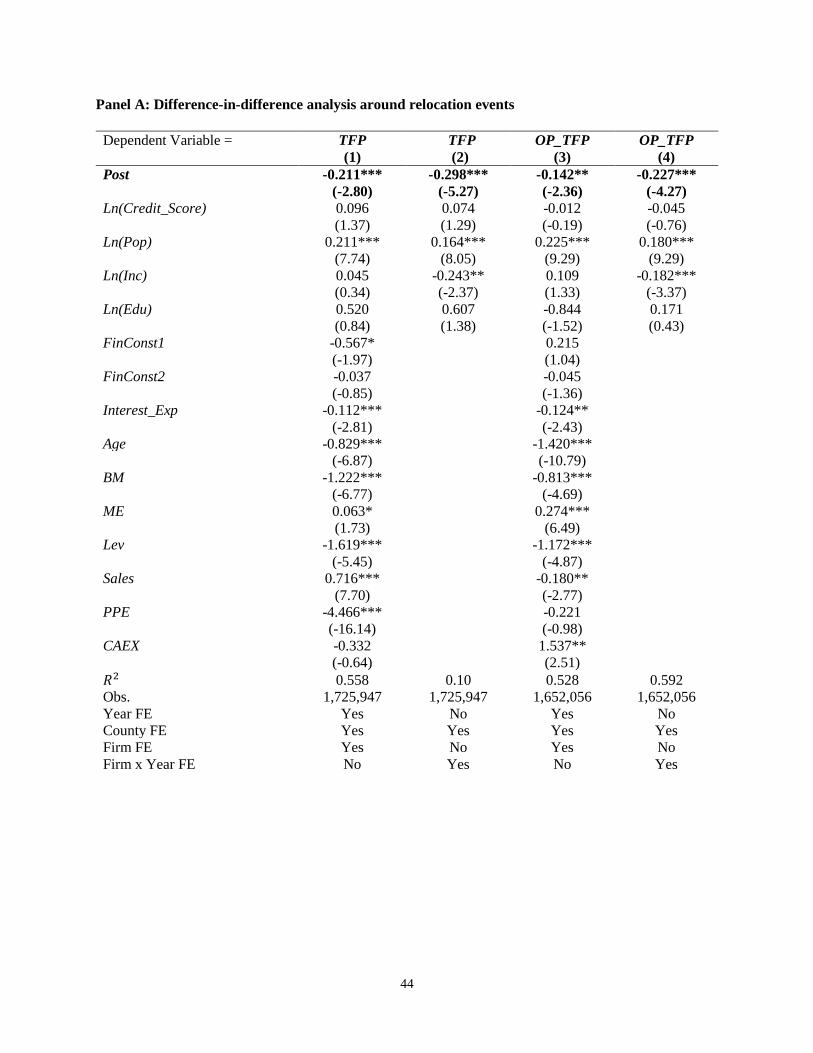
44

Panel A: Difference-in-difference analysis around relocation events

Dependent Variable = TFP

(1)

TFP

(2)

OP_TFP

(3)

OP_TFP

(4)

Post -0.211*** -0.298*** -0.142** -0.227***

(-2.80) (-5.27) (-2.36) (-4.27)

Ln(Credit_Score) 0.096 0.074 -0.012 -0.045

(1.37) (1.29) (-0.19) (-0.76)

Ln(Pop) 0.211*** 0.164*** 0.225*** 0.180***

(7.74) (8.05) (9.29) (9.29)

Ln(Inc) 0.045 -0.243** 0.109 -0.182***

(0.34) (-2.37) (1.33) (-3.37)

Ln(Edu) 0.520 0.607 -0.844 0.171

(0.84) (1.38) (-1.52) (0.43)

FinConst1 -0.567* 0.215

(-1.97) (1.04)

FinConst2 -0.037 -0.045

(-0.85) (-1.36)

Interest_Exp -0.112*** -0.124**

(-2.81) (-2.43)

Age -0.829*** -1.420***

(-6.87) (-10.79)

BM -1.222*** -0.813***

(-6.77) (-4.69)

ME 0.063* 0.274***

(1.73) (6.49)

Lev -1.619*** -1.172***

(-5.45) (-4.87)

Sales 0.716*** -0.180**

(7.70) (-2.77)

PPE -4.466*** -0.221

(-16.14) (-0.98)

CAEX -0.332 1.537**

(-0.64) (2.51)

𝑅2 0.558 0.10 0.528 0.592

Obs. 1,725,947 1,725,947 1,652,056 1,652,056

Year FE Yes No Yes No

County FE Yes Yes Yes Yes

Firm FE Yes No Yes No

Firm x Year FE No Yes No Yes

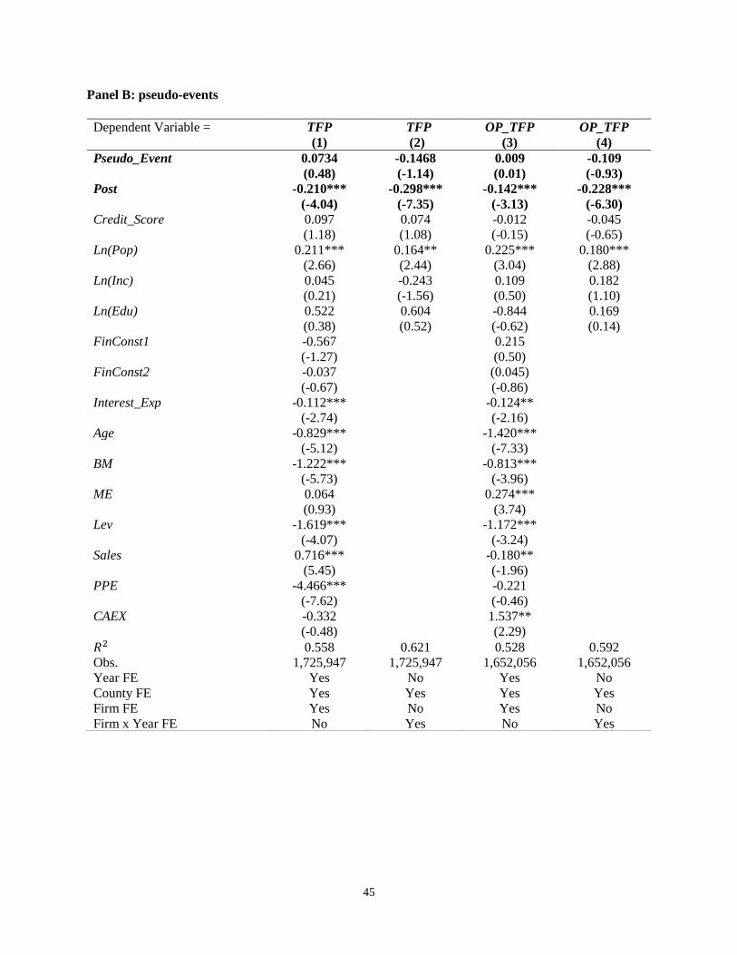
45

Panel B: pseudo-events


(1)

TFP

(2)

OP_TFP

(3)

OP_TFP

(4)

Pseudo_Event 0.0734 -0.1468 0.009 -0.109

(0.48) (-1.14) (0.01) (-0.93)

Post -0.210*** -0.298*** -0.142*** -0.228***

(-4.04) (-7.35) (-3.13) (-6.30)

Credit_Score 0.097 0.074 -0.012 -0.045

(1.18) (1.08) (-0.15) (-0.65)

Ln(Pop) 0.211*** 0.164** 0.225*** 0.180***

(2.66) (2.44) (3.04) (2.88)

Ln(Inc) 0.045 -0.243 0.109 0.182

(0.21) (-1.56) (0.50) (1.10)

Ln(Edu) 0.522 0.604 -0.844 0.169

(0.38) (0.52) (-0.62) (0.14)

FinConst1 -0.567 0.215

(-1.27) (0.50)

FinConst2 -0.037 (0.045)

(-0.67) (-0.86)

Interest_Exp -0.112*** -0.124**

(-2.74) (-2.16)

Age -0.829*** -1.420***

(-5.12) (-7.33)

BM -1.222*** -0.813***

(-5.73) (-3.96)

ME 0.064 0.274***

(0.93) (3.74)

Lev -1.619*** -1.172***

(-4.07) (-3.24)

Sales 0.716*** -0.180**

(5.45) (-1.96)

PPE -4.466*** -0.221

(-7.62) (-0.46)

CAEX -0.332 1.537**

(-0.48) (2.29)

𝑅2 0.558 0.621 0.528 0.592

Obs. 1,725,947 1,725,947 1,652,056 1,652,056





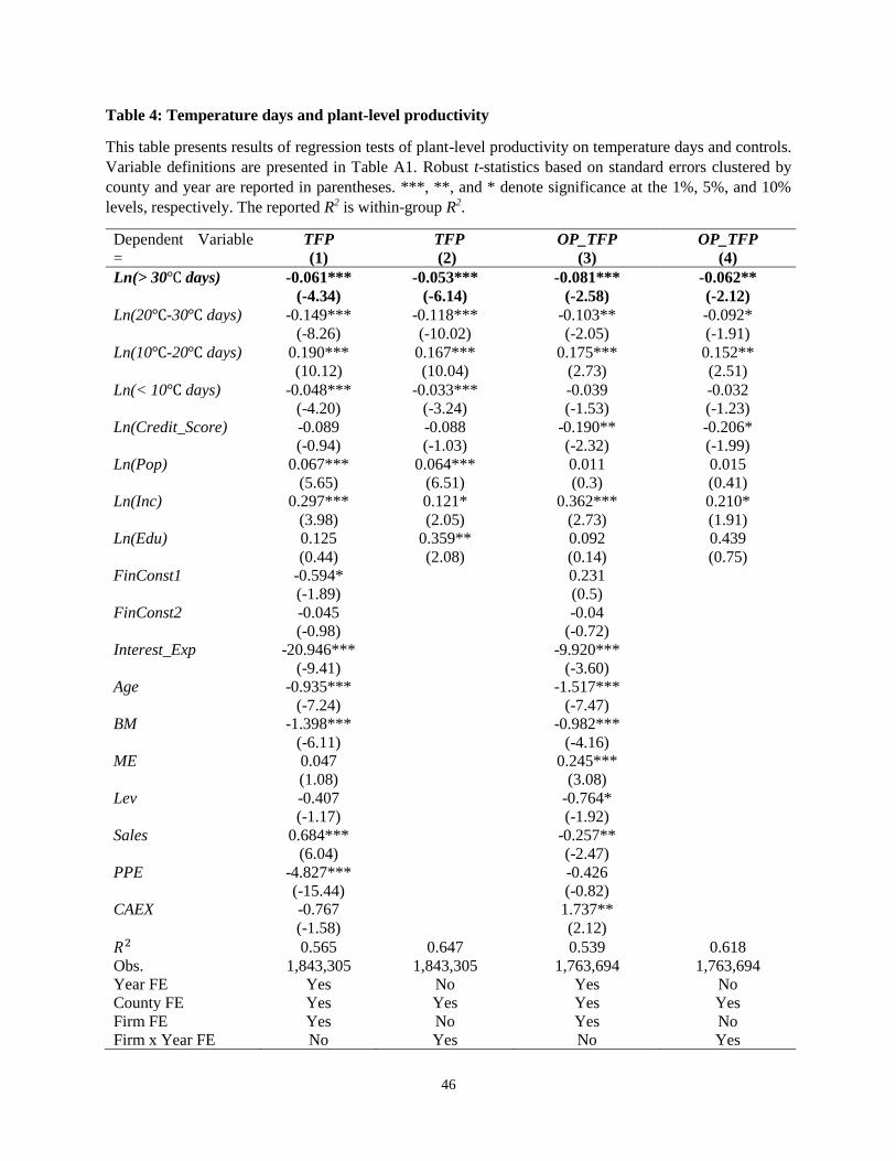
46

Table 4: Temperature days and plant-level productivity

This table presents results of regression tests of plant-level productivity on temperature days and controls.

Variable definitions are presented in Table A1. Robust t-statistics based on standard errors clustered by

county and year are reported in parentheses. ***, **, and * denote significance at the 1%, 5%, and 10%

levels, respectively. The reported R2 is within-group R2.

Dependent Variable

=

TFP

(1)

TFP

(2)

OP_TFP

(3)

OP_TFP

(4)

Ln(> 30℃ days) -0.061*** -0.053*** -0.081*** -0.062**

(-4.34) (-6.14) (-2.58) (-2.12)

Ln(20℃-30℃ days) -0.149*** -0.118*** -0.103** -0.092*

(-8.26) (-10.02) (-2.05) (-1.91)

Ln(10℃-20℃ days) 0.190*** 0.167*** 0.175*** 0.152**

(10.12) (10.04) (2.73) (2.51)

Ln(< 10℃ days) -0.048*** -0.033*** -0.039 -0.032

(-4.20) (-3.24) (-1.53) (-1.23)

Ln(Credit_Score) -0.089 -0.088 -0.190** -0.206*

(-0.94) (-1.03) (-2.32) (-1.99)

Ln(Pop) 0.067*** 0.064*** 0.011 0.015

(5.65) (6.51) (0.3) (0.41)

Ln(Inc) 0.297*** 0.121* 0.362*** 0.210*

(3.98) (2.05) (2.73) (1.91)

Ln(Edu) 0.125 0.359** 0.092 0.439

(0.44) (2.08) (0.14) (0.75)

FinConst1 -0.594* 0.231

(-1.89) (0.5)

FinConst2 -0.045 -0.04

(-0.98) (-0.72)

Interest_Exp -20.946*** -9.920***

(-9.41) (-3.60)

Age -0.935*** -1.517***

(-7.24) (-7.47)

BM -1.398*** -0.982***

(-6.11) (-4.16)

ME 0.047 0.245***

(1.08) (3.08)

Lev -0.407 -0.764*

(-1.17) (-1.92)

Sales 0.684*** -0.257**

(6.04) (-2.47)

PPE -4.827*** -0.426

(-15.44) (-0.82)

CAEX -0.767 1.737**

(-1.58) (2.12)

𝑅2 0.565 0.647 0.539 0.618

Obs. 1,843,305 1,843,305 1,763,694 1,763,694





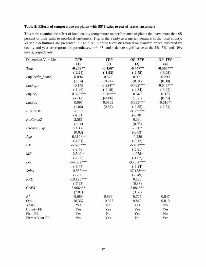
47

Table 5: Effects of temperature on plants with 95% sales to out-of-states customers

This table examine the effect of local county temperature on performance of plants that have more than 95

percent of their sales to non-local customers. Tmp is the yearly average temperature in the local county.

Variable definitions are presented in Table A1. Robust t-statistics based on standard errors clustered by

county and year are reported in parentheses. ***, **, and * denote significance at the 1%, 5%, and 10%

levels, respectively.


(1)

TFP

(2)

OP_TFP

(3)

OP_TFP

(4)

Tmp -0.209** -0.156* -0.447** -0.565***

(-2.24) (-1.93) (-2.75) (-3.02)

Ln(Credit_Score) 0.894 0.572 0.902 0.290

(1.16) (0.74) (0.91) (0.30)

Ln(Pop) -0.149 -0.234** -0.762*** -0.648***

(-1.46) (-2.18) (-4.34) (-3.22)

Ln(Inc) -0.522*** -0.615*** 0.545 0.373

(-3.12) (-4.06) (1.50) (0.74)

Ln(Edu) 0.097 0.0589 -0.635*** -0.616**

(1.06) (0.67) (-2.85) (-2.54)

FinConst1 -1.557 -8.689***

(-1.31) (-3.48)

FinConst2 2.581 0.330

(1.14) (0.08)

Interest_Exp 53.339 -3.307

(0.83) (-0.03)

Age -6.310*** -0.280

(-4.91) (-0.12)

BM -5.629*** -6.461***

(-8.48) (-5.81)

ME -2.549** -4.078*

(-2.06) (-1.87)

Lev -54.032*** -93.850***

(-6.44) (-5.14)

Sales -10.867*** -47.188***

(-3.66) (-8.49)

PPE -10.125*** 0.125

(-7.93) (0.38)

CAEX 7.966*** 2.081***

(2.87) (3.68)

𝑅2 0.689 0.636 0.725 0.647

Obs. 10,367 10,367 9,810 9,810





48

Table 6: Effects of temperature on special industries

The table reports results for regression tests of plant-level performance on temperature, indicators for

agriculture and outdoor industries, interactions between temperature and the two indicators, and controls.

Agriculture is an indicator variable equal to 1 for agricultural industries (those with SIC codes 100-799

according to Fama and French’s classification). Outdoor is an indicator variable equal to 1 for construction

and transportation industries (those with SIC codes 1500-2459 and 4000-4789 as per Fama and French’s

classification). Variable definitions are presented in Table A1. Robust t-statistics based on standard errors



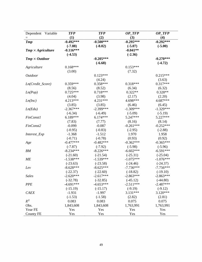
49

Dependent Variable

=

TFP

(1)

TFP

(2)

OP_TFP

(3)

OP_TFP

(4)

Tmp -0.492*** -0.500*** -0.295*** -0.292***

(-7.88) (-8.02) (-5.07) (-5.00)

Tmp × Agriculture -0.116*** -0.041**

(-4.53) (-2.36)

Tmp × Outdoor -0.205*** -0.270***

(-6.68) (-4.72)

Agriculture 0.168*** 0.153***

(3.00) (7.32)

Outdoor 0.123*** 0.215***

(4.24) (3.63)

Ln(Credit_Score) 0.359*** 0.358*** 0.318*** 0.317***

(8.56) (8.52) (6.34) (6.32)

Ln(Pop) 0.725*** 0.718*** 0.322** 0.328**

(4.04) (3.98) (2.17) (2.20)

Ln(Inc) 4.213*** 4.231*** 4.698*** 4.687***

(3.85) (3.85) (6.46) (6.45)

Ln(Edu) -2.367*** -2.399*** -1.309*** -1.329***

(-6.34) (-6.49) (-5.09) (-5.19)

FinConst1 6.189*** 6.174*** 5.247*** 5.227***

(7.83) (7.77) (8.16) (8.14)

FinConst2 -0.099 -0.087 -0.261*** -0.252***

(-0.95) (-0.83) (-2.95) (-2.88)

Interest_Exp -1.368 -1.512 1.970 1.958

(-0.71) (-0.78) (0.93) (0.92)

Age -0.477*** -0.482*** -0.362*** -0.365***

(-7.87) (-7.92) (-5.98) (-5.96)

BM -8.234*** -8.226*** -6.602*** -6.591***

(-21.60) (-21.54) (-25.31) (-25.04)

ME -1.538*** -1.539*** -1.075*** -1.076***

(-23.63) (-23.58) (-24.46) (-24.37)

Lev -8.628*** -8.625*** -7.736*** -7.756***

(-22.37) (-22.60) (-18.82) (-19.10)

Sales -2.620*** -2.617*** -2.863*** -2.863***

(-32.78) (-32.85) (-45.12) (-44.80)

PPE -4.691*** -4.653*** -2.511*** -2.487***

(-15.19) (-15.17) (-9.19) (-9.12)

CAEX -1.931 -1.997 3.131*** 3.120***

(-1.53) (-1.58) (2.82) (2.81)

𝑅2 0.083 0.083 0.075 0.075

Obs. 1,843,608 1,843,608 1,763,991 1,763,991

Year FE Yes Yes Yes Yes


50

Table 7: Temperature, innovation, and plant-level productivity

The table examines the effect of temperature on productivity of inventors at the establishment level. Panel

A presents results for regression tests of the natural logarithm of number of patents (Ln(Patents)) and

citation-weighted number of patents (TCW) on plant-level county temperature and controls. To measure

innovation at each plant, we first identify the location of each inventor in a firm. We then match the patent

ID of Kogan et al. (2017) with its inventor and the county of each plant from the NETS database to measure

the innovation at the inventor’s plant location. The sample period is 1969-2010. Variable definitions are

presented in Table A1. Panel B repeats the analysis of Panel A, except that it uses the sample without

establishments located in California. Panel C presents results for regression tests of the natural logarithm

of the average number of inventors in a county on average temperature and county-level controls.

Tmp_3year_Avg, Tmp_5year_Avg, and Tmp_10year_Avg are the 3-year, 5-year, and 10-year moving

averages (MA) of temperature, respectively. The dependent variables in Models (1), (2), and (3) are the

natural logarithm of 3-year, 5-year, 10-year moving averages of number of inventors in a county,

respectively. Education_Avg, Income_Avg, and Population_Avg are moving averages of county-level

education, income, and population, where the moving average window of each regression matches the

duration of the dependent variable. Panel D reports results for regression tests of temperature on

productivity of plants that are more dependent on innovative ability of inventors. To estimate a plant’s

performance sensitivity to innovation, we estimate a 10-year rolling regression of a plant’s TFP or OP_TFP

on the natural logarithm of number of patents (Ln(Patents)). The annual coefficient on Ln(Patents), denoted

as 𝛽𝑡𝑚𝑝𝑖𝑛𝑛𝑜, represents an plant’s performance sensitivity to productivity of inventors. In the second stage, we

regress a plant’s TFP or OP_TFP on temperature, 𝛽𝑡𝑚𝑝𝑖𝑛𝑛𝑜, interaction between the two variables, and controls

and report estimation results in Panel D. Robust t-statistics based on standard errors clustered by county

and year are reported in parentheses. ***, **, and * denote significance at the 1%, 5%, and 10% levels,

respectively.

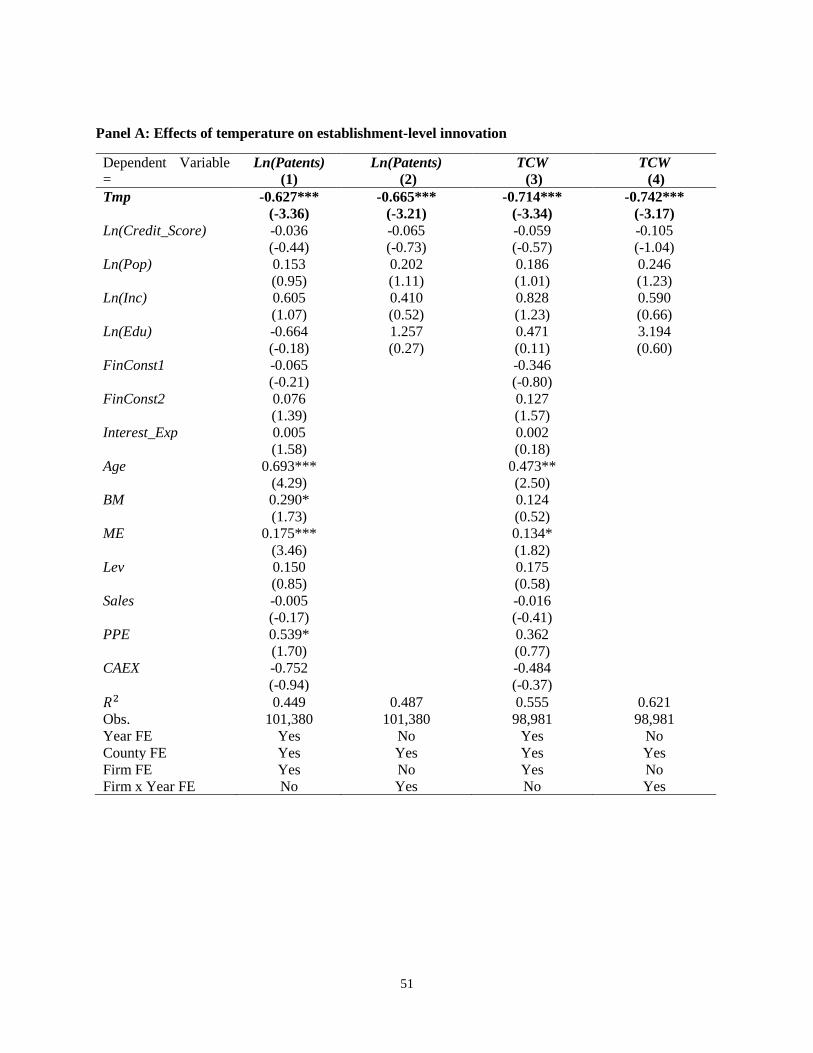
51

Panel A: Effects of temperature on establishment-level innovation

Dependent Variable

=

Ln(Patents)

(1)

Ln(Patents)

(2)

TCW

(3)

TCW

(4)

Tmp -0.627*** -0.665*** -0.714*** -0.742***

(-3.36) (-3.21) (-3.34) (-3.17)

Ln(Credit_Score) -0.036 -0.065 -0.059 -0.105

(-0.44) (-0.73) (-0.57) (-1.04)

Ln(Pop) 0.153 0.202 0.186 0.246

(0.95) (1.11) (1.01) (1.23)

Ln(Inc) 0.605 0.410 0.828 0.590

(1.07) (0.52) (1.23) (0.66)

Ln(Edu) -0.664 1.257 0.471 3.194

(-0.18) (0.27) (0.11) (0.60)

FinConst1 -0.065 -0.346

(-0.21) (-0.80)

FinConst2 0.076 0.127

(1.39) (1.57)

Interest_Exp 0.005 0.002

(1.58) (0.18)

Age 0.693*** 0.473**

(4.29) (2.50)

BM 0.290* 0.124

(1.73) (0.52)

ME 0.175*** 0.134*

(3.46) (1.82)

Lev 0.150 0.175

(0.85) (0.58)

Sales -0.005 -0.016

(-0.17) (-0.41)

PPE 0.539* 0.362

(1.70) (0.77)

CAEX -0.752 -0.484

(-0.94) (-0.37)

𝑅2 0.449 0.487 0.555 0.621

Obs. 101,380 101,380 98,981 98,981





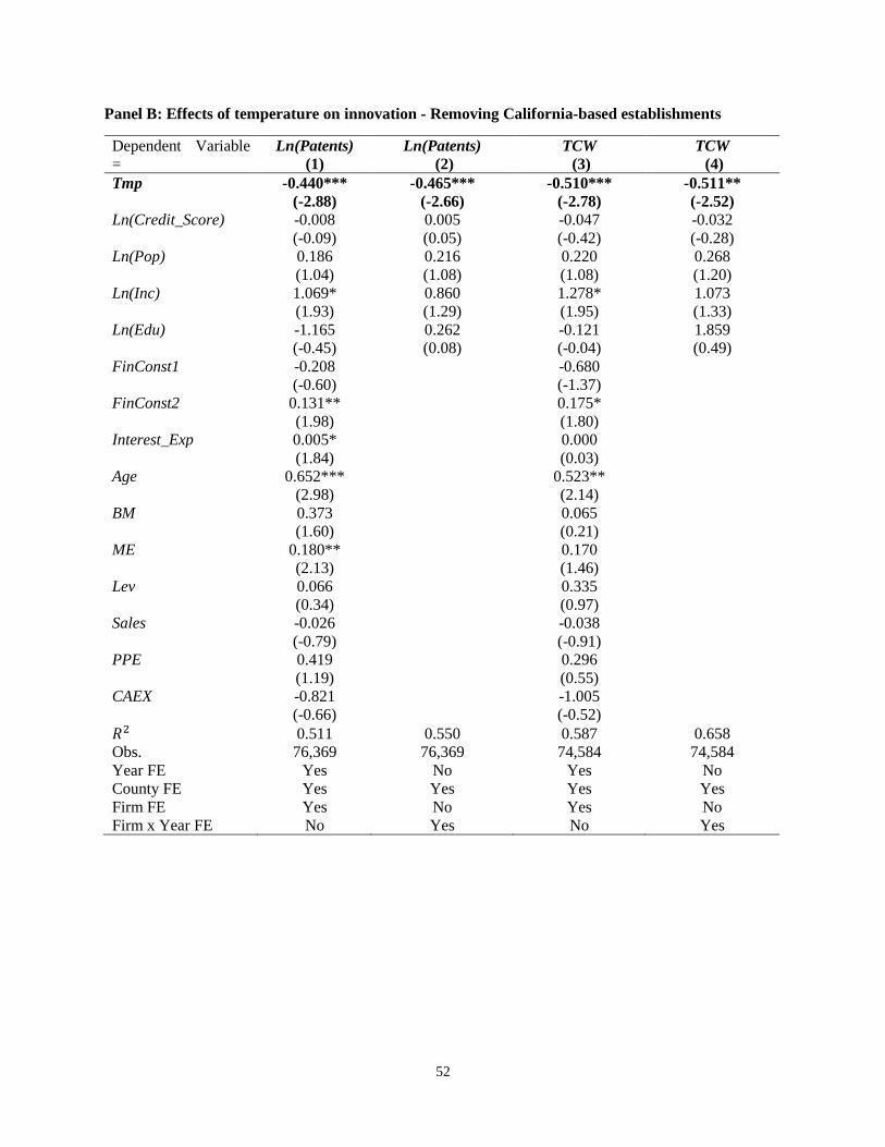
52

Panel B: Effects of temperature on innovation - Removing California-based establishments

Dependent Variable

=

Ln(Patents)

(1)

Ln(Patents)

(2)

TCW

(3)

TCW

(4)

Tmp -0.440*** -0.465*** -0.510*** -0.511**

(-2.88) (-2.66) (-2.78) (-2.52)

Ln(Credit_Score) -0.008 0.005 -0.047 -0.032

(-0.09) (0.05) (-0.42) (-0.28)

Ln(Pop) 0.186 0.216 0.220 0.268

(1.04) (1.08) (1.08) (1.20)

Ln(Inc) 1.069* 0.860 1.278* 1.073

(1.93) (1.29) (1.95) (1.33)

Ln(Edu) -1.165 0.262 -0.121 1.859

(-0.45) (0.08) (-0.04) (0.49)

FinConst1 -0.208 -0.680

(-0.60) (-1.37)

FinConst2 0.131** 0.175*

(1.98) (1.80)

Interest_Exp 0.005* 0.000

(1.84) (0.03)

Age 0.652*** 0.523**

(2.98) (2.14)

BM 0.373 0.065

(1.60) (0.21)

ME 0.180** 0.170

(2.13) (1.46)

Lev 0.066 0.335

(0.34) (0.97)

Sales -0.026 -0.038

(-0.79) (-0.91)

PPE 0.419 0.296

(1.19) (0.55)

CAEX -0.821 -1.005

(-0.66) (-0.52)

𝑅2 0.511 0.550 0.587 0.658

Obs. 76,369 76,369 74,584 74,584





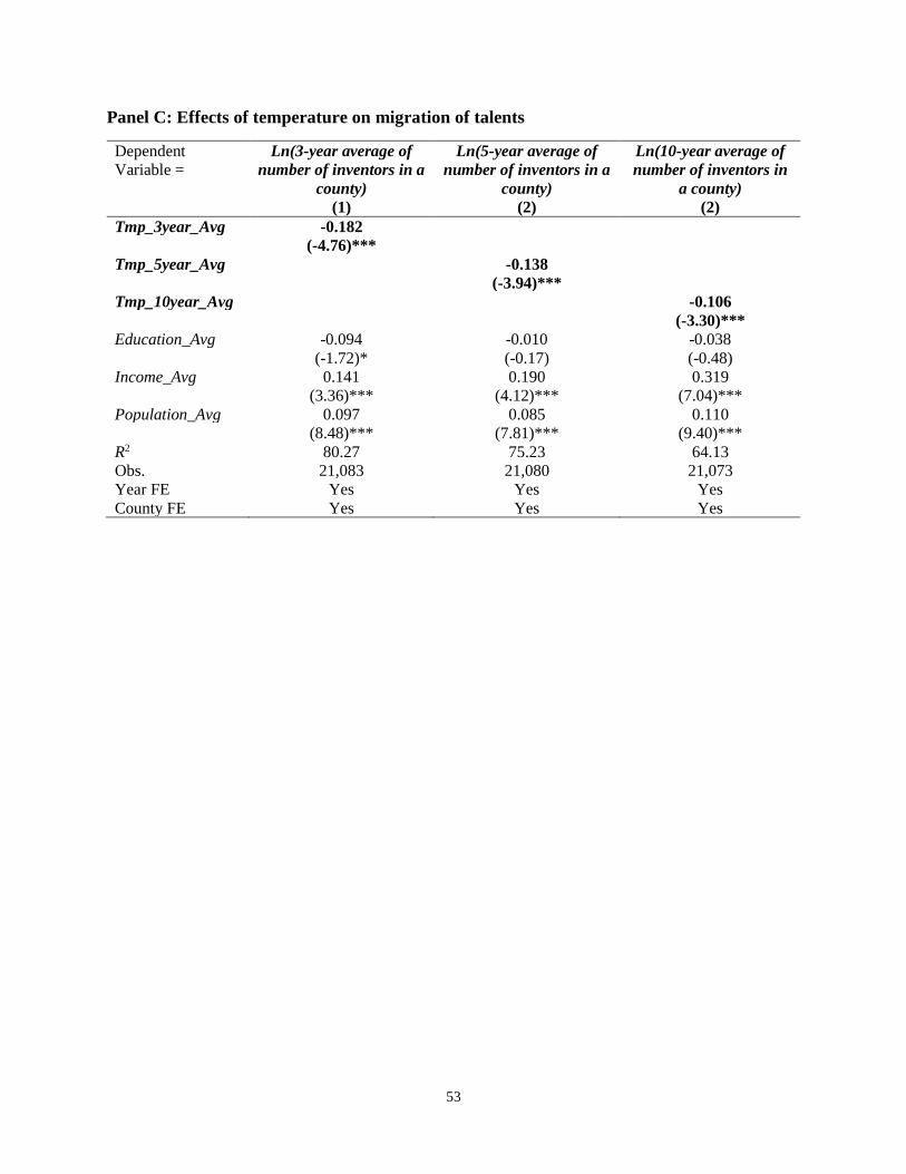
53

Panel C: Effects of temperature on migration of talents

Dependent

Variable =

Ln(3-year average of

number of inventors in a

county)


number of inventors in a

county)


number of inventors in

a county)

(1) (2) (2)

Tmp_3year_Avg -0.182

(-4.76)***


(-3.94)***


(-3.30)***

Education_Avg -0.094 -0.010 -0.038

(-1.72)* (-0.17) (-0.48)

Income_Avg 0.141 0.190 0.319

(3.36)*** (4.12)*** (7.04)***

Population_Avg 0.097 0.085 0.110

(8.48)*** (7.81)*** (9.40)***

R2 80.27 75.23 64.13

Obs. 21,083 21,080 21,073

Year FE Yes Yes Yes

County FE Yes Yes Yes

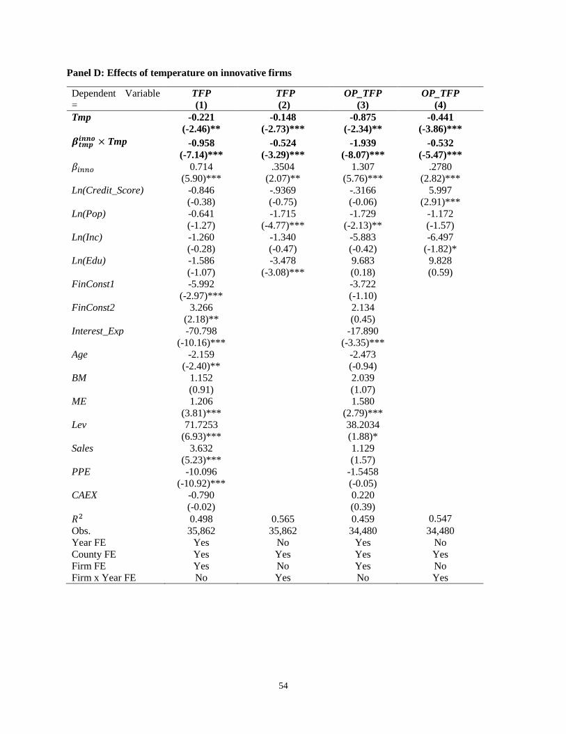
54

Panel D: Effects of temperature on innovative firms

Dependent Variable

=

TFP

(1)

TFP

(2)

OP_TFP

(3)

OP_TFP

(4)

Tmp -0.221 -0.148 -0.875 -0.441

(-2.46)** (-2.73)*** (-2.34)** (-3.86)***

𝜷𝒕𝒎𝒑𝒊𝒏𝒏𝒐 × Tmp -0.958 -0.524 -1.939 -0.532

(-7.14)*** (-3.29)*** (-8.07)*** (-5.47)***

𝛽𝑖𝑛𝑛𝑜 0.714 .3504 1.307 .2780

(5.90)*** (2.07)** (5.76)*** (2.82)***

Ln(Credit_Score) -0.846 -.9369 -.3166 5.997

(-0.38) (-0.75) (-0.06) (2.91)***

Ln(Pop) -0.641 -1.715 -1.729 -1.172

(-1.27) (-4.77)*** (-2.13)** (-1.57)

Ln(Inc) -1.260 -1.340 -5.883 -6.497

(-0.28) (-0.47) (-0.42) (-1.82)*

Ln(Edu) -1.586 -3.478 9.683 9.828

(-1.07) (-3.08)*** (0.18) (0.59)

FinConst1 -5.992 -3.722

(-2.97)*** (-1.10)

FinConst2 3.266 2.134

(2.18)** (0.45)

Interest_Exp -70.798 -17.890

(-10.16)*** (-3.35)***

Age -2.159 -2.473

(-2.40)** (-0.94)

BM 1.152 2.039

(0.91) (1.07)

ME 1.206 1.580

(3.81)*** (2.79)***

Lev 71.7253 38.2034

(6.93)*** (1.88)*

Sales 3.632 1.129

(5.23)*** (1.57)

PPE -10.096 -1.5458

(-10.92)*** (-0.05)

CAEX -0.790 0.220

(-0.02) (0.39)

𝑅2 0.498 0.565 0.459 0.547

Obs. 35,862 35,862 34,480 34,480





55

Table 8: Temperature, mental health, physical health, and plant-level productivity

This table examines whether plant’s productivity is more affected by temperature when the mental health

of residents in the local county is more sensitive to temperature. Panel A reports results for regressions of

productivity on temperature, a measure of sensitivity of suicide rate to temperature (denoted as 𝛽𝑡𝑚𝑝𝑠𝑢𝑖𝑐𝑖𝑑𝑒),

the interaction term between temperature and 𝛽𝑡𝑚𝑝𝑠𝑢𝑖𝑐𝑖𝑑𝑒, and controls. To compute 𝛽𝑡𝑚𝑝

𝑠𝑢𝑖𝑐𝑖𝑑𝑒 for a county in

a given year, we estimate 10-year rolling window regressions of county’s suicide rate on temperature in the

county. 𝛽𝑡𝑚𝑝𝑠𝑢𝑖𝑐𝑖𝑑𝑒 is the annual (time-series) coefficient on temperature obtained from these rolling

regressions. Panel B reports results for regressions of productivity on temperature, a measure of sensitivity

of hospital admissions to temperature of each county in California (denoted as 𝛽𝑡𝑚𝑝ℎ𝑜𝑠𝑝𝑖𝑡𝑎𝑙

), and controls.

Since only information on hospitals in California is publicly available, the sample for Panel B is restricted

to establishments in California. Moreover, since the data are available over the period 2010-2014 only, we

compute 𝛽𝑡𝑚𝑝ℎ𝑜𝑠𝑝𝑖𝑡𝑎𝑙

for a county by estimating a regression of the county’s average number of days admitted

to hospital per patient on temperature in the county using all data between 2010 and 2014. This gives an

estimate of 𝛽𝑡𝑚𝑝ℎ𝑜𝑠𝑝𝑖𝑡𝑎𝑙

for each county, which is the coefficient on temperature obtained from these county-

level regressions. We assume that 𝛽𝑡𝑚𝑝ℎ𝑜𝑠𝑝𝑖𝑡𝑎𝑙

is the same over the larger sample for a county. Other variable

definitions are presented in Table A1. Robust t-statistics based on standard errors clustered by county and

year are reported in parentheses. ***, **, and * denote significance at the 1%, 5%, and 10% levels,

respectively.

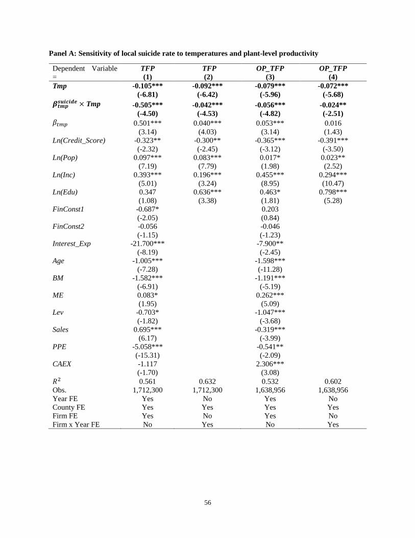
56

Panel A: Sensitivity of local suicide rate to temperatures and plant-level productivity

Dependent Variable

=

TFP

(1)

TFP

(2)

OP_TFP

(3)

OP_TFP

(4)

Tmp -0.105*** -0.092*** -0.079*** -0.072***

(-6.81) (-6.42) (-5.96) (-5.68)

𝜷𝒕𝒎𝒑𝒔𝒖𝒊𝒄𝒊𝒅𝒆 × Tmp -0.505*** -0.042*** -0.056*** -0.024**

(-4.50) (-4.53) (-4.82) (-2.51)

𝛽𝑡𝑚𝑝 0.501*** 0.040*** 0.053*** 0.016

(3.14) (4.03) (3.14) (1.43)

Ln(Credit_Score) -0.323** -0.300** -0.365*** -0.391***

(-2.32) (-2.45) (-3.12) (-3.50)

Ln(Pop) 0.097*** 0.083*** 0.017* 0.023**

(7.19) (7.79) (1.98) (2.52)

Ln(Inc) 0.393*** 0.196*** 0.455*** 0.294***

(5.01) (3.24) (8.95) (10.47)

Ln(Edu) 0.347 0.636*** 0.463* 0.798***

(1.08) (3.38) (1.81) (5.28)

FinConst1 -0.687* 0.203

(-2.05) (0.84)

FinConst2 -0.056 -0.046

(-1.15) (-1.23)

Interest_Exp -21.700*** -7.900**

(-8.19) (-2.45)

Age -1.005*** -1.598***

(-7.28) (-11.28)

BM -1.582*** -1.191***

(-6.91) (-5.19)

ME 0.083* 0.262***

(1.95) (5.09)

Lev -0.703* -1.047***

(-1.82) (-3.68)

Sales 0.695*** -0.319***

(6.17) (-3.99)

PPE -5.058*** -0.541**

(-15.31) (-2.09)

CAEX -1.117 2.306***

(-1.70) (3.08)

𝑅2 0.561 0.632 0.532 0.602

Obs. 1,712,300 1,712,300 1,638,956 1,638,956





57

Panel B: Sensitivity of local hospital admission rate to temperatures and plant-level productivity

Dependent Variable

=

TFP

(1)

TFP

(2)

OP_TFP

(3)

OP_TFP

(4)

Tmp -0.796*** -0.634*** -0.713*** -0.699***

(-3.24) (-3.03) (-4.16) (-2.65)

𝜷𝒕𝒎𝒑𝒉𝒐𝒔𝒑𝒊𝒕𝒂𝒍

× Tmp -0.235*** -0.146** -0.165** -0.168**

(-2.86) (-2.43) (-2.04) (-2.22)

𝛽𝑡𝑚𝑝 0.153** 0.054 0.053 0.047

(2.35) (1.28) (0.72) (0.92)

Ln(Credit_Score) -1.608* -1.959*** -2.499*** -3.027***

(-1.96) (-2.91) (-3.84) (-3.47)

Ln(Pop) -0.019 -0.177 -0.082 -0.086

(-0.03) (-0.27) (-0.53) (-0.11)

Ln(Inc) 0.305 0.274 0.396*** 0.229

(1.06) (1.34) (5.2) (0.97)

Ln(Edu) -5.867 -1.048 -1.207** -1.035

(-0.42) (-0.83) (-2.14) (-0.70)

FinConst1 -6.215 -2.499

(-1.56) (-1.43)

FinConst2 -0.112 0.235

(-0.24) (0.71)

Interest_Exp -11.781*** -4.478*

(-3.64) (-2.02)

Age -4.564*** -8.289***

(-3.49) (-9.24)

BM -6.982*** -5.450***

(-3.93) (-3.34)

ME 0.923 1.490***

(1.57) (3.43)

Lev -0.658 -4.220*

(-0.20) (-1.78)

Sales 3.904*** -1.218*

(3.99) (-1.99)

PPE -26.727*** 2.796*

(-5.86) (1.81)

CAEX -4.192 11.942**

(-0.69) (2.34)

𝑅2 0.581 0.640 0.553 0.618

Obs. 219,931 219,931 210,235 210,235





58

Table 9: Effects of temperature on firm-level Tobin’s Q

The table reports results for regressions of firm-level Peters and Taylor’s (2017) Tobin’s Q on plant-

weighted temperature and firm-level controls. Weighted temperature variables are computed as the

weighted average of temperature across the counties in which a firm has an operating plant, where the

weight is computed based on the economic size of each plant within the firm. Robust t-statistics based on

standard errors clustered by industry and year are reported in parentheses.

Dependent Variable = (1) (2) (3) (4)

Weighted_Tmp -0.227 -0.199

(-2.93)*** (-2.70)***

Weighted_Ln(>30 ℃

days) -0.070 -0.111

(-2.88)*** (-2.55)***

Weighted_Ln(20 ℃ -

30℃ days) 0.112 0.124

(3.81)*** (3.37)***

Weighted_Ln(10 ℃ -

20℃ days) 0.354 0.078

(5.97)*** (1.13)

Weighted_Ln(<10 ℃

days) 0.130 0.111

(1.70)* (1.21)

FinConst1 -1.346 -0.567 -1.236 -0.505

(-7.24)*** (-3.43)*** (-10.46)*** (-2.97)***

FinConst2 0.148 0.050 0.127 0.039

(9.26)*** (3.59)*** (12.57)*** (2.72)***

Interest_Exp -0.895 0.142 -0.818 0.098

(-1.40) (0.24) (-2.03)** (0.15)

Age -0.351 -0.881 -0.360 -0.877

(-7.09)*** (-9.45)*** (-5.81)*** (-7.41)***

BM -2.332 -1.407 -2.328 -1.407

(-19.53)*** (-15.63)*** (-16.60)*** (-10.36)***

ME 0.123 0.346 0.124 0.347

(18.72)*** (28.14)*** (14.99)*** (16.10)***

Lev -1.146 -0.992 -1.101 -0.988

(-16.51)*** (-14.79)*** (-27.26)*** (-14.14)***

Sales -0.341 -0.088 -0.318 -0.089

(-17.16)*** (-3.74)*** (-16.90)*** (-4.07)***

PPE -0.953 -1.293 -0.679 -1.291

(-13.58)*** (-15.19)*** (-25.36)*** (-16.96)***

CAEX 1.576 0.802 1.262 0.802

(8.34)*** (4.82)*** (10.49)*** (4.45)***

𝑅2 0.442 0.557 0.442 0.647

Obs. 62,011 62,011 61,953 61,953

Year FE Yes Yes Yes Yes


Firm FE No Yes No Yes

Industry FE Yes No Yes No

59

Table 10: Placebo analysis using temperature on weekends

This table examine the effect of weekend temperature on plant-level productivity and controls. Variable

definitions are presented in Table A1. Robust t-statistics based on standard errors clustered by county and

year are reported in parentheses. ***, **, and * denote significance at the 1%, 5%, and 10% levels,

respectively.


(1)

TFP

(2)

OP_TFP

(3)

OP_TFP

(4)

Weekend_Tmp 0.064 -0.031 -0.002 -0.024

(1.24) (-0.87) (-0.05) (-0.63)

Ln(Credit_Score) -1.788** -0.570* -1.760*** -1.262***

(-2.53) (-1.89) (-3.72) (-4.71)

Ln(Pop) 0.109*** 0.114*** 0.042 0.047*

(2.84) (2.99) (1.43) (1.99)

Ln(Inc) 0.328 0.385 -0.062 0.118

(0.31) (0.57) (-0.09) (0.26)

Ln(Edu) 0.240 0.635*** 0.760*** 0.803***

(0.80) (3.73) (4.08) (7.98)

FinConst1 0.980 0.741

(0.50) (0.72)

FinConst2 -0.463 -0.171

(-1.66) (-1.17)

Interest_Exp -63.354*** -23.108***

(-7.30) (-7.54)

Age -1.921*** -5.012***

(-3.98) (-10.49)

BM 2.702* 4.002***

(1.83) (5.241)

ME 1.542*** 2.659***

(4.32) (11.414)

Lev 39.355*** 14.859***

(8.04) (8.098)

Sales 4.205*** 1.601***

(6.79) (4.596)

PPE -20.875*** -5.188***

(-7.59) (-4.091)

CAEX -17.252*** 2.279

(-2.80) (0.965)

𝑅2 0.511 0.582 0.537 0.531

Obs. 1,843,607 1,843,607 1,763,991 1,763,991





60

Table 11: Controlling for other weather variables

The table presents results of regression tests of plant-level performance on temperature and additional

weather variables. Precipitation is the yearly average level of precipitation at the county level. Wind is the

natural logarithm of the yearly average wind speed at the county level. Evaporation is the yearly average

evaporation at the county level. Sun is the natural logarithm of average duration of sunshine in a year.

Definitions of other variables are presented in Table A1. Robust t-statistics based on standard errors



61

Dependent Variable

=

TFP

(1)

TFP

(2)

OP_TFP

(3)

OP_TFP

(4)

Tmp -0.152*** -0.163*** -0.417** -0.316**

(-4.01) (-5.89) (-2.35) (-2.37)

Precipitation 0.000 -0.000 -0.005 -0.004

(0.29) (-0.26) (-0.89) (-1.40)

Wind 0.166* -0.008 2.385** 0.237

(1.72) (-0.14) (2.36) (1.61)

Evaporation -0.019*** -0.004 -0.078 -0.013

(-4.33) (-1.64) (-1.65) (-1.16)

Sun 0.011** 0.002 0.122*** -0.001

(2.60) (0.42) (2.80) (-0.08)

Ln(Credit_Score) -0.086 -0.087 -0.409 -0.338**

(-0.92) (-1.03) (-1.70) (-2.14)

Ln(Pop) 0.211*** 0.161*** 0.198 0.312***

(8.24) (8.70) (1.58) (3.46)

Ln(Inc) 0.035 -0.328*** -2.407*** -0.536**

(0.26) (-3.02) (-4.69) (-2.07)

Ln(Edu) 0.133 0.461 5.076* 1.395

(0.21) (1.08) (1.89) (1.31)

FinConst1 -0.590* 0.687

(-1.88) (0.67)

FinConst2 -0.043 -0.172

(-0.92) (-1.16)

Interest_Exp -20.957*** -23.255***

(-9.43) (-7.52)

Age -0.935*** -5.070***

(-7.27) (-10.75)

BM -1.401*** 4.132***

(-6.12) (5.39)

ME 0.047 2.700***

(1.09) (11.51)

Lev -0.414 15.036***

(-1.19) (8.19)

Sales 0.686*** 1.624***

(6.07) (4.63)

PPE -4.822*** -5.156***

(-15.42) (-4.12)

CAEX -0.786 2.435

(-1.63) (1.04)

𝑅2 0.565 0.648 0.535 0.632

Obs. 1,842,834 1,842,834 1,762,912 1,762,912





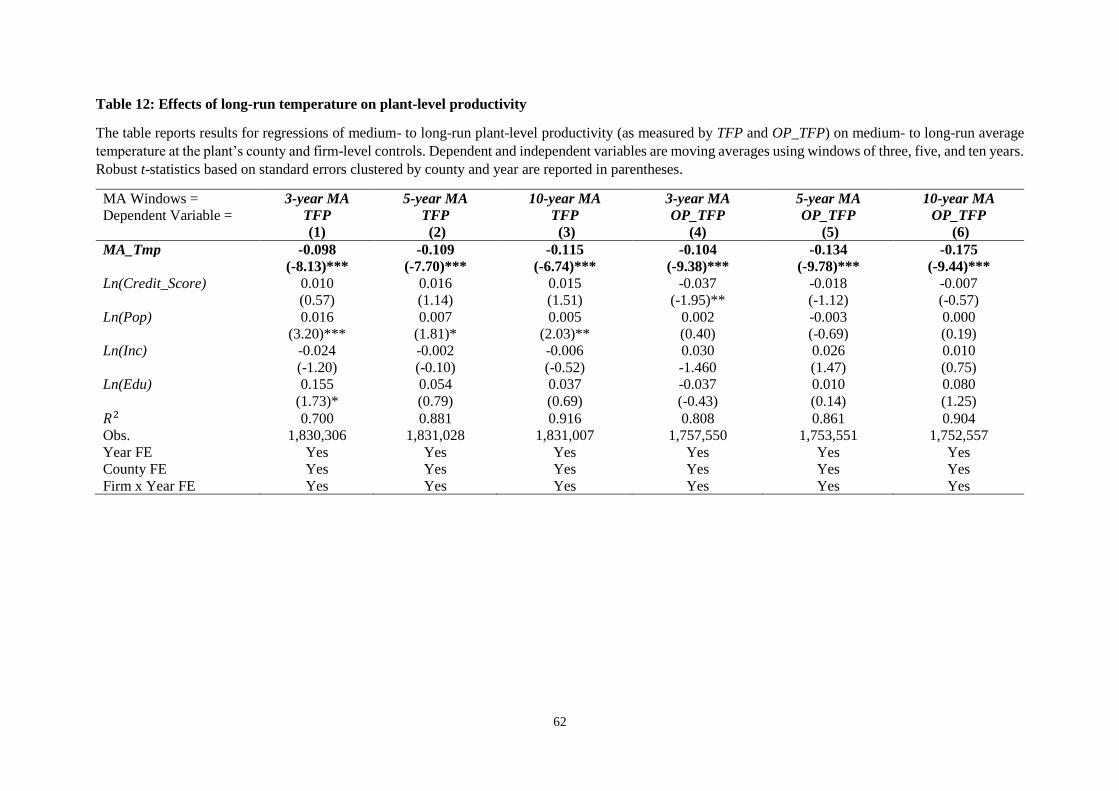
62

Table 12: Effects of long-run temperature on plant-level productivity

The table reports results for regressions of medium- to long-run plant-level productivity (as measured by TFP and OP_TFP) on medium- to long-run average

temperature at the plant’s county and firm-level controls. Dependent and independent variables are moving averages using windows of three, five, and ten years.

Robust t-statistics based on standard errors clustered by county and year are reported in parentheses.

MA Windows =

Dependent Variable =

3-year MA

TFP

(1)

5-year MA

TFP

(2)

10-year MA

TFP

(3)

3-year MA

OP_TFP

(4)

5-year MA

OP_TFP

(5)

10-year MA

OP_TFP

(6)

MA_Tmp -0.098 -0.109 -0.115 -0.104 -0.134 -0.175

(-8.13)*** (-7.70)*** (-6.74)*** (-9.38)*** (-9.78)*** (-9.44)***

Ln(Credit_Score) 0.010 0.016 0.015 -0.037 -0.018 -0.007

(0.57) (1.14) (1.51) (-1.95)** (-1.12) (-0.57)

Ln(Pop) 0.016 0.007 0.005 0.002 -0.003 0.000

(3.20)*** (1.81)* (2.03)** (0.40) (-0.69) (0.19)

Ln(Inc) -0.024 -0.002 -0.006 0.030 0.026 0.010

(-1.20) (-0.10) (-0.52) -1.460 (1.47) (0.75)

Ln(Edu) 0.155 0.054 0.037 -0.037 0.010 0.080

(1.73)* (0.79) (0.69) (-0.43) (0.14) (1.25)

𝑅2 0.700 0.881 0.916 0.808 0.861 0.904

Obs. 1,830,306 1,831,028 1,831,007 1,757,550 1,753,551 1,752,557

Year FE Yes Yes Yes Yes Yes Yes

County FE Yes Yes Yes Yes Yes Yes

Firm x Year FE Yes Yes Yes Yes Yes Yes

63

Appendix

Table A1: Variable definitions

Variable Definition

TFP Plant-level (total factor productivity (𝑇𝐹𝑃) for each individual plant is

the estimated residual from the following regression:

𝐿𝑛(𝑦𝑖𝑗𝑡) = 𝛼𝑗𝑡 + 𝑏𝑗𝑡 ln(𝐾𝑖𝑗𝑡) + 𝑐𝑗𝑡 ln(𝐿𝑖𝑗𝑡) + 𝑑𝑗𝑡 ln(𝑀𝑖𝑗𝑡) + 𝜀𝑖𝑗𝑡

where plant-level labor (𝐿) is the number of employees in each plant by

provided by NETS and plant-level output (𝑦) is the plant-level sales

obtained from NETS. We approximate plant-level capital (𝐾) as the

plant’s economic weight multiplied by the firm-level property, plant and

equipment (PPE) obtained from Compustat annual file. A plant’s

economic weight within a firm is equal to 1

2

𝑒𝑚𝑝𝑙𝑜𝑦𝑒𝑒𝑠𝑖,𝑝,𝑡

𝑒𝑚𝑝𝑙𝑜𝑦𝑒𝑒𝑠𝑖,𝑡𝑜𝑡𝑎𝑙,𝑡+

1

2

𝑠𝑎𝑙𝑒𝑠𝑖,𝑝,𝑡

𝑠𝑎𝑙𝑒𝑠𝑠𝑖,𝑡𝑜𝑡𝑎𝑙,𝑡, where 𝑒𝑚𝑝𝑙𝑜𝑦𝑒𝑒𝑠𝑖,𝑝,𝑡 and 𝑠𝑎𝑙𝑒𝑠𝑖,𝑝,𝑡 are the employment

and sales levels at plant 𝑝 of firm 𝑖. Similarly, to compute plant-level

input material (𝑀), we multiply the plant’s weight by the firm-level cost

of goods sold obtained from Compustat.

OP_TFP TFP measure estimated using Olley and Pakes (1996) method, which

corrects for the fact that plants simultaneously choose the level of inputs

as they choose their outputs. For example, firms tend to increase the use

of inputs when they observe a positive production shock. Olley and

Pakes (1996) use investment as a proxy variable, which is determined by

the shock to production and existing capital stock. We approximate

investment at the plant level as the plant’s economic weight multiplied

by the firm-level investment obtained from Compustat annual file. Using

this instrument, we follow Olley and Pakes (1996) and estimate the

production function for each industry separately.

Tmp Temperature (in degrees Celsius) computed as the average of daily

average temperature over a firm’s fiscal year at the county where the

firm’s headquarter locates.

Weighted_Tmp Weighted Average temperatures (in degrees Celsius) across the counties

where the firm’s plant is located. The weight is equal to 0.5 ×𝑠𝑎𝑙𝑒𝑠𝑝,𝑖



𝑡𝑜𝑡𝑎𝑙 𝑒𝑚𝑝𝑙𝑜𝑦𝑒𝑒𝑠𝑖, where 𝑠𝑎𝑙𝑒𝑠𝑝,𝑖 and 𝑒𝑚𝑝𝑙𝑜𝑦𝑒𝑒𝑠𝑝,𝑖

are sales and number of employees at plant p of firm i; 𝑡𝑜𝑡𝑎𝑙 𝑠𝑎𝑙𝑒𝑠𝑖 and

𝑡𝑜𝑡𝑎𝑙 𝑒𝑚𝑝𝑙𝑜𝑦𝑒𝑒𝑠𝑖 are total sales and employees across all plants of the

firm.

Ln(< 10℃ days) The natural logarithm of one plus number of days over a firm’s fiscal

year when the daily temperature is below 10℃.

Ln(10℃-20℃ days) The natural logarithm of one plus number of days over a firm’s fiscal

year when the daily temperature is between 10℃ and 20℃.

Ln(20℃-30℃ days) The natural logarithm of one plus number of days over a firm’s fiscal

year when the daily temperature is between 20℃ and 30℃.

Ln(> 30℃ days) The natural logarithm of one plus number of days over a firm’s fiscal

year when the daily temperature is above 30℃.

64

Ln(< 10℃ days_w) The natural logarithm of the weighted average of one plus number of

days across all the plants of the firms over a firm’s fiscal year when the

daily temperature is below 10℃ in each plant’s location. The weight is

equal to 0.5 ×𝑠𝑎𝑙𝑒𝑠𝑝,𝑖



𝑡𝑜𝑡𝑎𝑙 𝑒𝑚𝑝𝑙𝑜𝑦𝑒𝑒𝑠𝑖, where 𝑠𝑎𝑙𝑒𝑠𝑝,𝑖 and

𝑒𝑚𝑝𝑙𝑜𝑦𝑒𝑒𝑠𝑝,𝑖 are sales and number of employees at plant p of firm i;

𝑡𝑜𝑡𝑎𝑙 𝑠𝑎𝑙𝑒𝑠𝑖 and 𝑡𝑜𝑡𝑎𝑙 𝑒𝑚𝑝𝑙𝑜𝑦𝑒𝑒𝑠𝑖 are total sales and employees

across all plants of the firm.

Ln(10℃-20℃

days_w)

The natural logarithm of the weighted average of one plus number of


daily temperature is between 10℃ and 20℃ in each plant’s location. The

weight is equal to 0.5 ×𝑠𝑎𝑙𝑒𝑠𝑝,𝑖



𝑡𝑜𝑡𝑎𝑙 𝑒𝑚𝑝𝑙𝑜𝑦𝑒𝑒𝑠𝑖, where

𝑠𝑎𝑙𝑒𝑠𝑝,𝑖 and 𝑒𝑚𝑝𝑙𝑜𝑦𝑒𝑒𝑠𝑝,𝑖 are sales and number of employees at plant

p of firm i; 𝑡𝑜𝑡𝑎𝑙 𝑠𝑎𝑙𝑒𝑠𝑖 and 𝑡𝑜𝑡𝑎𝑙 𝑒𝑚𝑝𝑙𝑜𝑦𝑒𝑒𝑠𝑖 are total sales and

employees across all plants of the firm.

Ln(20℃-30℃

days_w)

The natural logarithm of the weighted average of one plus number of


daily temperature is between 20℃ and 30℃ in each plant’s location. The

weight is equal to 0.5 ×𝑠𝑎𝑙𝑒𝑠𝑝,𝑖



𝑡𝑜𝑡𝑎𝑙 𝑒𝑚𝑝𝑙𝑜𝑦𝑒𝑒𝑠𝑖, where

𝑠𝑎𝑙𝑒𝑠𝑝,𝑖 and 𝑒𝑚𝑝𝑙𝑜𝑦𝑒𝑒𝑠𝑝,𝑖 are sales and number of employees at plant

p of firm i; 𝑡𝑜𝑡𝑎𝑙 𝑠𝑎𝑙𝑒𝑠𝑖 and 𝑡𝑜𝑡𝑎𝑙 𝑒𝑚𝑝𝑙𝑜𝑦𝑒𝑒𝑠𝑖 are total sales and

employees across all plants of the firm.

Ln(> 30℃ days_w) The natural logarithm of the weighted average of one plus number of

days across all the plants of the firm over its fiscal year when the daily

temperature is above 30℃ in each plant’s location. The weight is equal

to 0.5 ×𝑠𝑎𝑙𝑒𝑠𝑝,𝑖



𝑡𝑜𝑡𝑎𝑙 𝑒𝑚𝑝𝑙𝑜𝑦𝑒𝑒𝑠𝑖, where 𝑠𝑎𝑙𝑒𝑠𝑝,𝑖 and

𝑒𝑚𝑝𝑙𝑜𝑦𝑒𝑒𝑠𝑝,𝑖 are sales and number of employees at plant p of firm i;

𝑡𝑜𝑡𝑎𝑙 𝑠𝑎𝑙𝑒𝑠𝑖 and 𝑡𝑜𝑡𝑎𝑙 𝑒𝑚𝑝𝑙𝑜𝑦𝑒𝑒𝑠𝑖 are total sales and employees

across all plants of the firm.

LnPop Natural logarithm of county-level population.

LnInc Natural logarithm of county-level average income.

Ln(Credit_Score) Natural logarithm of plant-level credit score, which ranges from 0 to 100

and is rated by credit rating agency Dun and Bradstreet.

CAEX Capital expenditure defined as capital expenditures divided by total

assets.

PPE Asset tangibility computed as net properties, plants and equipment

scaled by total assets.

FinConst1 Hoberg and Maksimovic’s (2015) text-based financial constraints. Firms

with higher values of FinConst1 are more similar to a set of firms known

to be at risk of delaying their investments due to issues with liquidity.

65

FinConst2 An indicator variable that takes a value of 1 for firm-year with missing

FinConst1. According to Hoberg and Maksimovic: “if a researcher

wishes to include the constraint variables in a regression where some

observations are missing (and the researcher wants to not lose

observations and thus control for the missing values), we recommend

(A) including a dummy in the regression for observations where the

given variable is missing and (B) then it is ok to set the constraint

variable to zero for these missing observations.”

Interest_Exp Interest expense measured as the ratio of total interest expense over

total sales.

Lev The ratio of long-term debt over book value of equity.

Age The natural logarithm of one plus number of years since the firm has its

listed price in the CRSP database.

BM The natural logarithm of book-to-market ratio.

ME The natural logarithm of the firm’s market equity measured at the end

of the fiscal year.

Sales The natural logarithm of net sales.

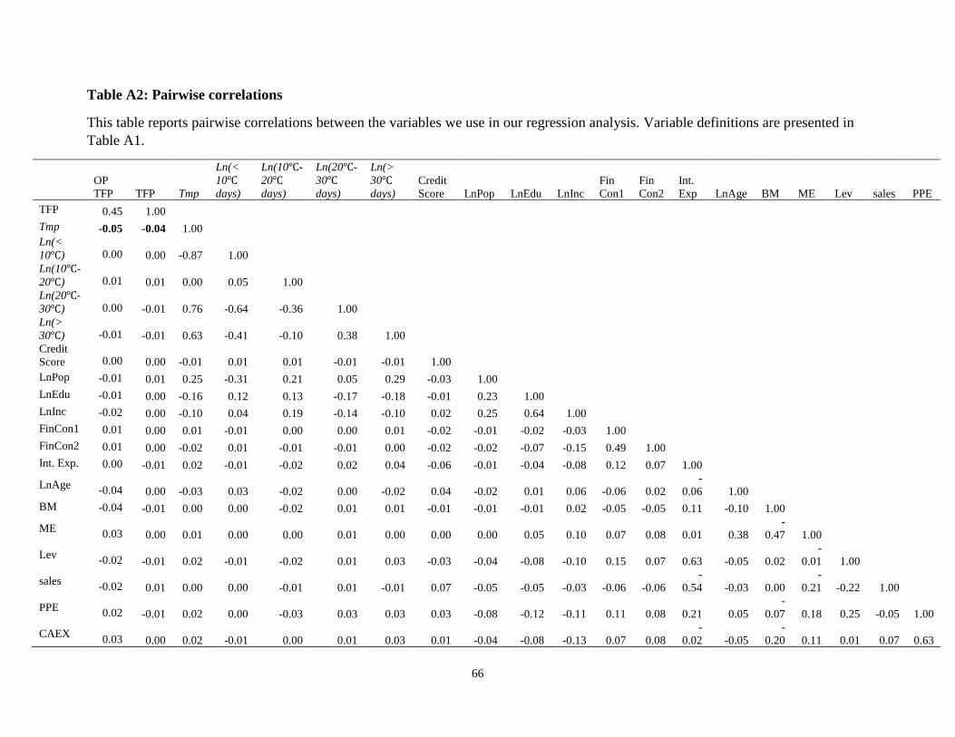
66

Table A2: Pairwise correlations

This table reports pairwise correlations between the variables we use in our regression analysis. Variable definitions are presented in

Table A1.

OP

TFP TFP Tmp

Ln(<

10℃

days)

Ln(10℃-

20℃

days)

Ln(20℃-

30℃

days)

Ln(>

30℃

days)

Credit

Score LnPop LnEdu LnInc

Fin

Con1

Fin

Con2

Int.

Exp LnAge BM ME Lev sales PPE

TFP 0.45 1.00 Tmp -0.05 -0.04 1.00 Ln(<

10℃) 0.00 0.00 -0.87 1.00 Ln(10℃-

20℃) 0.01 0.01 0.00 0.05 1.00 Ln(20℃-

30℃) 0.00 -0.01 0.76 -0.64 -0.36 1.00 Ln(>

30℃) -0.01 -0.01 0.63 -0.41 -0.10 0.38 1.00 Credit

Score 0.00 0.00 -0.01 0.01 0.01 -0.01 -0.01 1.00 LnPop -0.01 0.01 0.25 -0.31 0.21 0.05 0.29 -0.03 1.00 LnEdu -0.01 0.00 -0.16 0.12 0.13 -0.17 -0.18 -0.01 0.23 1.00 LnInc -0.02 0.00 -0.10 0.04 0.19 -0.14 -0.10 0.02 0.25 0.64 1.00 FinCon1 0.01 0.00 0.01 -0.01 0.00 0.00 0.01 -0.02 -0.01 -0.02 -0.03 1.00 FinCon2 0.01 0.00 -0.02 0.01 -0.01 -0.01 0.00 -0.02 -0.02 -0.07 -0.15 0.49 1.00 Int. Exp. 0.00 -0.01 0.02 -0.01 -0.02 0.02 0.04 -0.06 -0.01 -0.04 -0.08 0.12 0.07 1.00

LnAge -0.04 0.00 -0.03 0.03 -0.02 0.00 -0.02 0.04 -0.02 0.01 0.06 -0.06 0.02

-

0.06 1.00 BM -0.04 -0.01 0.00 0.00 -0.02 0.01 0.01 -0.01 -0.01 -0.01 0.02 -0.05 -0.05 0.11 -0.10 1.00

ME 0.03 0.00 0.01 0.00 0.00 0.01 0.00 0.00 0.00 0.05 0.10 0.07 0.08 0.01 0.38

-

0.47 1.00

Lev -0.02 -0.01 0.02 -0.01 -0.02 0.01 0.03 -0.03 -0.04 -0.08 -0.10 0.15 0.07 0.63 -0.05 0.02

-

0.01 1.00

sales -0.02 0.01 0.00 0.00 -0.01 0.01 -0.01 0.07 -0.05 -0.05 -0.03 -0.06 -0.06

-

0.54 -0.03 0.00

-

0.21 -0.22 1.00

PPE 0.02 -0.01 0.02 0.00 -0.03 0.03 0.03 0.03 -0.08 -0.12 -0.11 0.11 0.08 0.21 0.05

-

0.07 0.18 0.25 -0.05 1.00

CAEX 0.03 0.00 0.02 -0.01 0.00 0.01 0.03 0.01 -0.04 -0.08 -0.13 0.07 0.08

-

0.02 -0.05

-

0.20 0.11 0.01 0.07 0.63

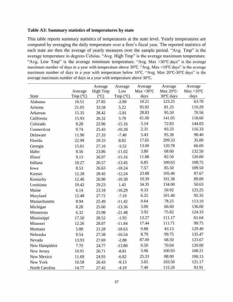
67

Table A3: Summary statistics of temperatures by state

This table reports summary statistics of temperatures at the state level. Yearly temperatures are

computed by averaging the daily temperature over a firm’s fiscal year. The reported statistics of

each state are then the average of yearly measures over the sample period. “Avg. Tmp” is the

average temperature in degrees Celsius. “Avg. High Tmp” is the average maximum temperature.

“Avg. Low Tmp” is the average minimum temperature. “Avg. Max >30℃ days” is the average

maximum number of days in a year with temperature above 30℃. “Avg. Max <10℃ days” is the average

maximum number of days in a year with temperature below 10℃. “Avg. Max 20℃-30℃ days” is the

average maximum number of days in a year with temperature above 30℃.

State

Average

Tmp (℃)

Average

High Tmp

(℃)

Average

Low

Tmp (℃)

Average

Max >30℃

days

Average

Max 20℃-

30℃ days

Average

Max <10℃

days

Alabama 16.51 27.85 -2.89 10.21 123.25 63.70

Arizona 21.05 33.58 5.22 95.92 81.25 110.29

Arkansas 15.35 28.42 -5.81 28.83 95.50 70.56

California 15.93 26.32 5.79 61.00 141.05 118.60

Colorado 8.28 22.96 -15.16 3.14 72.83 144.03

Connecticut 9.74 25.43 -10.28 2.31 93.33 116.33

Delaware 11.96 27.33 -7.40 3.43 95.38 98.40

Florida 22.99 29.33 8.82 17.65 209.33 35.00

Georgia 15.61 27.16 -3.52 13.00 120.78 66.00

Idaho 8.56 23.86 -11.02 3.80 68.60 132.50

Illinoi 9.13 26.97 -15.16 11.88 82.50 120.00

Indiana 10.27 26.57 -13.45 6.85 100.63 108.75

Iowa 8.53 26.63 -18.24 7.57 85.50 109.50

Kansas 12.28 28.45 -12.24 23.88 105.46 87.67

Kentucky 12.46 26.90 -10.30 10.39 101.38 89.00

Louisiana 19.42 29.23 1.43 34.35 134.00 50.63

Maine 6.14 23.18 -16.29 0.33 50.92 123.25

Maryland 12.48 27.72 -7.19 6.25 101.40 95.35

Massachusetts 8.94 25.49 -11.42 0.64 78.25 113.10

Michigan 8.28 25.60 -13.36 3.00 66.60 136.00

Minnesota 6.32 25.98 -21.48 3.92 75.82 124.33

Mississippi 17.50 28.52 -1.93 13.27 111.17 61.64

Missouri 12.26 28.07 -11.84 17.44 111.71 99.75

Montana 5.88 21.28 -18.63 0.88 43.13 129.40

Nebraska 9.54 27.38 -16.54 8.79 99.75 135.47

Nevada 13.93 27.69 -2.88 87.00 68.50 123.67

New Hampshire 7.70 24.77 -13.80 0.50 70.04 120.00

New Jersey 10.91 26.71 -8.81 3.96 100.93 108.21

New Mexico 11.69 24.93 -6.82 25.33 88.00 106.15

New York 10.58 26.43 -9.13 3.65 103.50 121.17

North Carolina 14.77 27.42 -4.19 7.40 115.20 83.91

https://www.infoplease.com/world/states/massachusetts

https://www.infoplease.com/world/states/mississippi

68

North Dakota 4.38 25.03 -24.58 2.63 39.73 132.00

Ohio 9.87 25.84 -12.60 3.00 95.00 114.50

Oklahoma 15.09 29.51 -7.84 35.20 112.33 72.25

Oregon 10.73 23.64 -2.75 2.80 58.21 121.16

Pennsylvania 10.67 26.25 -9.60 3.36 96.42 114.00

Rhode Island 9.13 24.74 -11.09 0.44 76.41 115.25

South Carolina 15.97 27.82 -2.39 11.40 112.31 64.13

South Dakota 6.84 25.61 -20.28 5.58 55.80 115.22

Tennessee 14.21 27.16 -6.98 20.38 116.77 78.07

Texas 19.12 30.18 -0.43 62.50 139.70 75.75

Utah 7.80 22.76 -11.94 16.44 60.36 120.21

Vermont 6.03 23.76 -17.78 0.38 42.53 114.45

Virginia 12.92 27.35 -6.71 6.60 124.55 90.43

Washington 9.91 22.01 -3.95 5.22 84.89 123.33

West Virginia 11.02 25.48 -10.57 2.04 63.00 91.00

Wisconsin 7.04 25.38 -18.00 3.28 63.44 124.43

Wyoming 5.97 21.66 -18.62 30.50 37.67 133.41

Documents

Temperature and Productivity: Evidence from Plant-level Data