Embed Size (px)
Citation preview

Barcelona GSE Working Paper Series
Working Paper nº 736
Agricultural Productivity and Structural Transformation. Evidence from Brazil
Paula Bustos Bruno Caprettini Jacopo Ponticelli
This version: June 2015
(December 2014)
Agricultural Productivity and Structural Transformation.
Evidence from Brazil∗
Paula Bustos Bruno Caprettini Jacopo Ponticelli†
First Draft: July 2012
This Draft: June 2015
Abstract
We study the effects of the adoption of new agricultural technologies on structural transfor-
mation. To guide empirical work, we present a simple model where the effect of agricultural
productivity on industrial development depends on the factor bias of technical change. We test
the predictions of the model by studying the introduction of genetically engineered soybean
seeds in Brazil, which had heterogeneous effects on agricultural productivity across areas with
different soil and weather characteristics. We find that technical change in soy production was
strongly labor saving and led to industrial growth, as predicted by the model.
Keywords: Agricultural Productivity, Structural Transformation, Industrial Development, La-
bor Saving Technical Change, Genetically Engineered Soy.
JEL Classification: F16, F43, 014, Q16.
∗We received valuable comments from David Atkin, Francisco Buera, Vasco Carvalho, Gino Gancia, Gene Gross-man, Juan Carlos Hallak, Chang-Tai Hsieh, Joseph Kaboski, Nina Pavcnik, Joao Pinho de Melo, Silvana Tenreyro,Jaume Ventura, Kei-Mu Yi and participants at presentations held at Pontificia Universidade Catolica de Rio deJaneiro, Fundaçao Getulio Vargas, CREI, UPF, LSE, Universidad Torcuato di Tella, Harvard University, BrownUniversity, MIT, Chicago Booth, Federal Reserve Bank of New York, CEMFI, Toulouse School of Economics, YaleUniversity, Columbia University, Stanford University, Dartmouth College, Northwestern University, CopenhagenBusiness School, University of Southern California, SED annual meeting, CEPR ESSIM, CEPR ERWIT, BarcelonaGSE Summer Forum, Princeton IES Summer Workshop, AEA Annual Meeting, NBER SI International Trade andInvestment, NBER SI Development and Entrepreneurship, NBER SI Development Economics and LACEA. We ac-knowledge financial support from the Private Enterprise Development in Low-Income Countries Project by the CEPRand UK Department for International Development.†Bustos: Princeton University, CREI and UPF, [email protected]. Caprettini: Universitat Pom-
peu Fabra, [email protected]. Ponticelli: University of Chicago Booth School of Business, [email protected].
1 Introduction
The early development literature documented that the growth path of most advanced economies
was accompanied by a process of structural transformation. As economies develop, the share of
agriculture in employment falls and workers migrate to cities to find employment in the industrial
and service sectors [Clark (1940), Lewis (1954), Kuznets (1957)]. These findings suggest that iso-
lating the forces that can give rise to structural transformation is key to our understanding of the
development process. In particular, scholars have argued that increases in agricultural productivity
are an essential condition for economic development, based on the experience of England during the
industrial revolution.1 Classical models of structural transformation formalize their ideas by show-
ing how productivity growth in agriculture can release labor or generate demand for manufacturing
goods.2 However, several scholars noted that the positive effects of agricultural productivity on
industrialization occur only in closed economies, while in open economies a comparative advantage
in agriculture can slow down industrial growth.3 Despite the richness of the theoretical literature,
there is scarce direct empirical evidence testing the mechanisms proposed by these models.4
In this paper we provide direct empirical evidence on the effects of technical change in agriculture
on the industrial sector by studying the recent widespread adoption of new agricultural technologies
in Brazil. First, we analyze the effects of the adoption of genetically engineered soybean seeds (GE
soy). This new technology requires less labor per unit of land to yield the same output. Thus, it
can be characterized as labor-augmenting technical change. In addition, we study the effects of the
introduction of a second harvesting season for maize (milho safrinha). This technique permits to
grow two crops a year, effectively increasing the land endowment. Thus, it can be characterized as
land-augmenting technical change. The simultaneous expansion of these two crops allows to assess
the effect of agricultural productivity on structural transformation in open economies.
To guide empirical work, we build a simple model describing a two-sector small open economy
where technical change in agriculture can be factor biased. The model predicts that a Hicks-
neutral increase in agricultural productivity induces a reduction in the size of the industrial sector
as labor reallocates towards agriculture, as in classical open economy models such as Matsuyama
(1992). Similar results are obtained when technical change is land-augmenting. However, if land
1See, for example, Rosenstein-Rodan (1943), Nurkse (1953), Lewis (1954), Rostow (1960).2See Baumol (1967), Murphy, Shleifer, Vishny (1989), Kongsamut, Rebelo and Xie (2001), Gollin, Parente and
Rogerson (2002), Ngai and Pissarides (2007).3See Mokyr (1976), Field (1978), Wright (1979), Corden and Neary (1982), Krugman (1987), and Matsuyama
(1992).4Empirical studies of structural transformation include Foster and Rosenszweig (2004, 2008), Nunn and Qian
(2011), Michaels, Rauch and Redding (2012), Hornbeck and Keskin (2012). We discuss this literature in more detailbelow.
1
and labor are strong complements in agricultural production, labor-augmenting technical change
reduces labor demand in agriculture and causes workers to reallocate towards manufacturing. In
sum, the model predicts that the effects of agricultural productivity on structural transformation
in open economies depend on the factor-bias of technical change.
In a first analysis of the data we find that regions where the area cultivated with soy expanded
experienced an increase in agricultural output per worker, a reduction in labor intensity in agri-
culture and an expansion in industrial employment. These correlations are consistent with the
theoretical prediction that the adoption of labor-augmenting agricultural technologies reduces la-
bor demand in the agricultural sector and induces the reallocation of workers towards the industrial
sector. However, causality could run in the opposite direction. For example: an increase in produc-
tivity in the industrial sector could increase labor demand and wages, inducing agricultural firms
to switch to less labor intensive crops, like soy.
We propose to establish the direction of causality by using two sources of exogenous variation
in the profitability of technology adoption. First, in the case of GE soy, as the technology was
invented in the U.S. in 1996, and legalized in Brazil in 2003, we use this last date as our source of
variation across time. Second, as the new technology had a differential impact on yields depending
on geographical and weather characteristics, we use differences in soil suitability across regions as
our source of cross-sectional variation. Similarly, in the case of maize, we exploit the timing of
expansion of second-harvest maize and cross-regional differences in soil suitability.
We obtain an exogenous measure of technological change in agriculture by using estimates of
potential soil yields across geographical areas of Brazil from the FAO-GAEZ database. These
yields are calculated by incorporating local soil and weather characteristics into a model that
predicts the maximum attainable yields for each crop in a given area. Potential yields are a source
of exogenous variation in agricultural productivity because they are a function of weather and soil
characteristics, not of actual yields in Brazil. In addition, the database reports potential yields
under traditional and new agricultural technologies. Thus, we exploit the predicted differential
impact of the new technology on yields across geographical areas in Brazil as our source of cross-
sectional variation in agricultural productivity. Note that this empirical strategy relies on the
assumption that although goods can move across geographical areas of Brazil, labor markets are
local due to limited labor mobility. This research design allows us to investigate whether exogenous
shocks to local agricultural productivity lead to changes in the size of the local industrial sector.
We use municipalities as our geographical unit of observation, which are assumed to behave as the
small open economy described in the model.
We find that municipalities where the new technology is predicted to have a higher effect on
2
potential yields of soy did experience a larger expansion of the area planted with GE soy. In
addition, these regions experienced increases in the value of agricultural output per worker and
reductions in labor intensity measured as employment per hectare. Besides, these regions experi-
enced faster employment growth and wage reductions in the industrial sector. Interestingly, the
effects of technology adoption are different for maize. Regions where the FAO potential maize yields
are predicted to increase the most when switching from the traditional to the new technology did
indeed experience a higher increase in the area planted with maize. However, they also experienced
increases in labor intensity, reductions in industrial employment and increases in wages.
The different effects of technological change in agriculture documented for GE soy and maize
indicate that the factor-bias of technical change is a key determinant of the relationship between
agricultural productivity and structural transformation in open economies. Land-augmenting tech-
nical change, the case of second-harvest maize, leads to an increase in the marginal product of
labor in agriculture and a reduction in industrial employment. However, labor-augmenting techni-
cal change, the case of GE soy, leads to a reduction in the marginal product of labor in agriculture
and employment growth of the industrial sector. Thus, in what follows we refer to labor-augmenting
technical change as labor-saving.5
Our estimates can be used to quantify the effect of factor-biased agricultural technical change
on structural transformation. In particular, we compute the elasticity of sectoral employment
shares to changes in agricultural productivity induced by soy technical change: 1 percent increase
in agricultural labor productivity leads to a 0.16 percentage points decrease in the agricultural
employment share and an increase in the manufacturing employment share of a similar magnitude.
These estimates can be used to understand to what extent the observed differences in the speed of
structural transformation across Brazilian municipalities can be explained by labor-saving technical
change in soy. In the year 2000, the average municipality had employment shares in agriculture
and manufacturing of 38 and 10 percent, respectively. During the next decade, the degree of
labor reallocation across sectors varied extensively across municipalities. Our estimates imply
that labor-saving technical change in soy can explain 24 percent of the observed differences in the
reduction of the agricultural employment share across Brazilian municipalities and 31 percent of
the corresponding differences in the growth of the manufacturing employment share.
We complement our findings with an analysis of the service sector. For this purpose, we extend
the theoretical model by incorporating non-traded services. A central feature of the analysis is the
distinction between two effects of agricultural technical change: the supply effect and the demand
effect. In the case of land-augmenting technical change, the first effect is generated by the increase
5A formal definition of labor-saving technical change is contained in Section 3.
3
in the marginal product of labor in the agricultural sector, which draws workers out of other sectors.
The second effect is generated by the higher income resulting from technical change in agriculture
which leads to increased demand for non-traded services. Both effects lead to a reallocation of labor
away from the manufacturing sector. However, when technical change is labor-saving, the supply
effect releases agricultural workers. As a result, the net effect of agricultural technical change on
industrialization depends on the relative strength of the supply and demand effects. In addition, the
demand effect is only driven by an increase in land rents. Thus, its strength depends on the extent
to which land-owners consume services in the region where their land is located. Our empirical
results imply that in regions more affected by labor-saving technical change labor reallocated from
agriculture to manufacturing and not towards services. Our interpretation of these findings is that
the differences-in-differences empirical strategy is well suited to identify the supply effect to the
extent that labor markets are local. However, our model suggests that it might not be suitable to
identify the demand effect if land owners do not reside locally or consume services in other regions.
Thus, a further investigation of the effect of agricultural technical change on the service sector is
left for future work.
Finally, we assess the robustness of our estimates to a number of deviations from our baseline
framework. First, estimates are stable when we allow municipalities with different initial levels
of development to be on differential structural transformation trends. Second, we obtain similar
estimates in the subsample of Brazilian municipalities where the agricultural frontier did not ex-
pand. Third, contemporaneous migration patterns are consistent with the predictions of the model:
there is out (in) migration in areas more affected by labor-augmenting (land-augmenting) technical
change. Fourth, our estimates are not driven by pre-existing trends in manufacturing employment
nor migration flows. Fifth, our results are robust to using a larger unit of observation, micro-
regions. Sixth, at least 60 percent of our estimated effect of agricultural technical change on the
manufacturing employment share is not driven by the processing of soy and maize in downstream
industries nor larger agricultural sector demand for manufacturing inputs. Seventh, our estimates
are not driven by contemporaneous changes in commodity prices. Finally, our main results remain
statistically significant when we correct standard errors to account for spatial correlation.
Related Literature
There is a long tradition in economics of studying the links between agricultural productivity and
industrial development. Nurkse (1953), Schultz (1953) and Rostow (1960) argued that agricultural
productivity growth was an essential precondition for the industrial revolution. Classical models
of structural transformation formalized their ideas by proposing two main mechanisms through
which agricultural productivity can speed up industrial growth in closed economies. First, the
4

demand channel: agricultural productivity growth rises income per capita, which generates de-
mand for manufacturing goods if preferences are non-homothetic [Murphy, Shleifer, Vishny (1989),
Kongsamut, Rebelo and Xie (2001), Gollin, Parente and Rogerson (2002)]. The higher relative
demand for manufactures generates a reallocation of labor away from agriculture. Second, the sup-
ply channel: if productivity growth in agriculture is faster than in manufacturing and these goods
are complements in consumption, then the relative demand of agriculture does not grow as fast
as productivity and labor reallocates towards manufacturing [Baumol (1967), Ngai and Pissarides
(2007)].6
The view that agricultural productivity can generate manufacturing growth was challenged by
scholars studying industrialization experiences in open economies. These scholars argued that high
agricultural productivity can retard industrial growth as labor reallocates towards the comparative
advantage sector [Mokyr (1976), Field (1978) and Wright (1979)]. Their ideas were formalized by
Matsuyama (1992) who showed that the demand and supply channels are not operative in a small
open economy that faces a perfectly elastic demand for both goods at world prices. The open
economy model we present in this paper differs from Matsuyama’s in one key dimension. In his
model, there is only one input to production thus technical change is, by definition, Hicks-neutral.
In our model there are two factors, land and labor, and the two are complements in agricultural
production. Thus technical change can be factor-biased. In this setting, a new prediction emerges:
when technical change is labor augmenting, an increase in agricultural productivity leads to a
reallocation of labor towards the industrial sector even in open economies.7
Our work also builds on the empirical literature studying the links between agricultural pro-
ductivity and economic development.8 The closest precedent to our work is Foster and Rosenzweig
(2004, 2008) who study the effects of the adoption of high-yielding-varieties (HYV) of corn, rice,
sorghum, and wheat during the Green Revolution in India. To guide empirical work, they present
a model in which agricultural and manufacturing goods are tradable and technical change is Hicks-
neutral. Consistent with their model, they find that villages with higher improvements in crop
yields experienced lower manufacturing growth. Our findings are in line with theirs in the case
of maize, for which technical change is land-augmenting. However, we find the opposite effects
6Another mechanism generating a reallocation of labor from agriculture to manufacturing is faster growth in therelative supply of one production factor when there are differences in factor intensity across sectors [See Caselli andColeman (2001), and Acemoglu and Guerrieri (2008)]. For a recent survey of the structural transformation literaturesee Herrendorf, Valentinyi and Rogerson (2013).
7This prediction rests on the assumptions that land and labor are strong complements in agricultural production,and land is only used in the agricultural sector. This last assumption is not necessary to obtain the prediction. Tosee this, refer to the general discussion of the effects of technical change in an open economy with two goods and twofactors in Findlay and Grubert (1959).
8This literature is surveyed by Syrquin (1988) and Foster and Rosensezweig (2008).
5
in the case of soy, for which technical change is labor saving. Thus, relative to theirs, our work
highlights the importance of the factor-bias of technical change in shaping the relationship between
agricultural productivity and industrial development in open economies.
Our model is related to the literature on the Dutch Disease: Corden and Neary (1982) and
Krugman (1987). In particular, Corden and Neary consider a three-sector open economy model
with non-traded goods. One of the traded sectors is extractive and experiences a boom, which
leads to de-industrialization and an expansion of the service sector. We build on their distinction
between two effects of the boom: the spending effect and the resource movement effect, which we
call the demand and supply effects. Our setting differs in that we consider labor-saving technical
change which reduces the marginal product of labor in the booming sector, agriculture. Thus, in
our model the net effect of agricultural technical change on industrialization depends on the relative
strength of these effects.
Our research also connects to the literature studying the role of manufacturing in economic
development. This literature has shown that a reallocation of labor into manufacturing can increase
aggregate productivity: first, when labor productivity is lower in agriculture than in the rest of the
economy [Gollin, Parente and Rogerson (2002), Lagakos and Waugh (2013) and Gollin, Lagakos
and Waugh (2014)]; second, when the manufacturing sector is characterized by economies of scale
generated by on-the-job accumulation of human capital such as learning-by-doing [Krugman (1987),
Lucas (1988), Matsuyama (1992)].
Finally, our work is related to recent empirical papers studying the effects of agricultural pro-
ductivity on urbanization [Nunn and Qian (2011)], the links between structural transformation and
urbanization [Michaels, Rauch and Redding (2012)], the effects of agriculture on local economic
activity [Hornbeck and Keskin (2012)], and the role of out-migration from rural areas in favoring
the adoption of capital-intensive agricultural technologies [Hornbeck and Naidu (2014)].
The remaining of the paper is organized as follows. Section 2 gives background information
on agriculture in Brazil. Section 3 presents the theoretical model. Section 4 describes the data.
Section 5 presents the empirical strategy and results. Section 6 shows a set of robustness checks on
our main results. Section 7 concludes.
2 Agriculture in Brazil
In this section we provide background information on recent technological developments in Brazilian
agriculture. In particular, we focus on two new agricultural technologies for the cultivation of soy
and maize. The first is the use of genetically engineered (GE) seeds in soy cultivation. The second
6

is the introduction of a second harvesting season in maize during the same agricultural year, which
requires the use of advanced cultivation techniques.
2.1 Technical Change in Soy: Genetically Engineered Seeds
The main advantage of GE soy seeds relative to traditional seeds is that they are herbicide resistant,
which facilitates the use of no-tillage planting techniques.9 The planting of traditional seeds is
preceded by soil preparation in the form of tillage, the operation of removing the weeds in the
seedbed that would otherwise crowd out the crop or compete with it for water and nutrients.
In contrast, planting GE soy seeds requires no tillage, as the application of herbicide selectively
eliminates all unwanted weeds without harming the crop. As a result, GE soy seeds can be applied
directly on last season’s crop residue, allowing farmers to save on production costs since less labor
is required per unit of land to obtain the same output.10
The first generation of GE soy seeds, the Roundup Ready (RR) variety, was commercially
released in the U.S. in 1996 by the agricultural biotechnology firm Monsanto. In 1998, the Brazilian
National Technical Commission on Biosecurity (CTNBio) authorized Monsanto to field-test GE
soy in Brazil for 5-years as a first step before commercialization. Finally, in 2003, the Brazilian
government legalized the use of GE soy seeds.11 Prior to legalization, smuggling of GE soy seeds
from Argentina was detected since 2001 according to the Foreign Agricultural Service of the United
States Department of Agriculture (USDA, 2001).
The new technology spread quickly: in 2006 GE seeds were planted in 46.4% of the area
cultivated with soy in Brazil, according to the last Agricultural Census (IBGE, 2006, p.144). In
the following years the technology continued spreading to the point that, according to the Foreign
Agricultural Service of the USDA, it covered 85% of the area planted with soy in Brazil by the
9Genetic engineering (GE) techniques allow a precise alteration of a plant’s traits. This allows to target a singleplant’s trait, facilitating the development of plant characteristics with a precision not attainable through traditionalplant breeding. In the case of herbicide resistant GE soy seeds, soy genes were altered to include those of a bacteriathat was herbicide resistant.10GE soybeans seeds allow farmers to adopt a new set of techniques that lowers labor requirement for several
reasons. First, since GE soybeans are resistant to herbicides, weed control can be done more flexibly. Herbicides canbe applied at any time during the season, even after the emergence of the plant. Second, GE soybeans are resistantto a specific herbicide (glyphosate), which needs fewer applications: fields cultivated with GE soybeans require anaverage of 1.55 sprayer trips against 2.45 of conventional soybeans (Duffy and Smith, 2001; Fernandez-Cornejo et al.,2002). Third, no-tillage production techniques require less labor. This is because the application of chemicals needsfewer and shorter trips than tillage. In addition, no-tillage allows greater density of the crop on the field (Hugginsand Reganold, 2008). Finally, farmers that adopt GE soybeans report gains in the time to harvest (Duffy and Smith,2001). These cost savings might explain why the technology spread fast, even though experimental evidence in theU.S. reports no improvements in yield with respect to conventional soybeans (Fernandez-Cornejo and Caswell, 2006)11 In 2003, Brazilian law 10.688 allowed the commercialization of GE soy for one harvesting season, requiring farmers
to burn all unsold stocks after the harvest. This temporary measure was renewed in 2004. Finally, in 2005, law 11.105—the New Bio-Safety Law —authorized production and commercialization of GE soy in its Roundup Ready variety(art. 35).
7

2011-2012 harvesting season (USDA, 2012).
The timing of adoption of GE soy seeds coincides with an increase in labor productivity in soy
production and a fast expansion in the area planted with soy in Brazil. Figure 1(a) documents
the evolution of soy production per worker between 1980 and 2011. As the Figure shows, labor
productivity in soy production has been increasing in Brazil since the early 1990s, and accelerated
sharply in the early 2000s: soy production per worker went from 100 tonnes per worker in 2003
to around 300 tonnes per worker in 2011. Labor productivity growth was accompanied by an
expansion in area planted with soy. Table 1 reports land use by agricultural activity according to
the 1996 and 2006 Agricultural Censuses. It shows that the area cultivated with seasonal crops
increased by 10.4 million hectares between 1996 and 2006.12 Out of these, 6.4 million hectares were
converted to soy cultivation. Similarly, Figure 1(b) shows that the area planted with soy has been
growing since the 1980s, and experienced a sharp acceleration in the early 2000s.13
The adoption of GE soy can affect labor demand in the agricultural sector through two channels:
the within-crop and the across-crop effects. The first effect is due to a reduction in the amount
of agricultural workers per hectare required to cultivate soy: labor intensity of soy production fell
from 29 workers per 1000 hectares in 1996 to 18 workers per 1000 hectares in 2006 (Table 2). The
timing of this change in labor intensity is illustrated by Figure 1(c), which shows a sharp increase
in the area planted per worker in soy production in the early 2000s.14 This reduction in labor
intensity entirely offset the potential increase in labor demand for soy due to the expansion in
the area planted: Figure 1(d) shows that employment in soy production experienced a constant
decrease during the period under study.
In turn, the across-crop effect is due to the expansion of soy cultivation over areas previously
devoted to other crops. This effect reduces the labor intensity of production in the agricultural sec-
tor because soy production is one of the least labor-intensive agricultural activities: its production
12Seasonal crops are those produced from plants that need to be replanted after each harvest, such as soy andmaize.13Yearly data on area planted are from the CONAB survey. This is a survey of farmers and agronomists conducted
by an agency of the Brazilian Ministry of Agriculture to monitor the annual harvests of major crops in Brazil (seeSection A2 of the Appendix for a detailed description). We use data from the CONAB survey purely to illustrate thetiming of the evolution of aggregate agricultural outcomes during the period under study. In the empirical analysis,instead, we rely exclusively on data from the Agricultural Censuses which covers all farms in the country and it isrepresentative at municipality level.14Figure 1(c) displays yearly data on area planted with soy from the CONAB survey and yearly data on employment
in soy production from the PNAD survey. Table 2 instead is based on data on area planted and employment fromthe Agricultural Censuses of 1996 and 2006. Notice that the decrease in labor intensity in soy production between1996 and 2006 implied by Figure 1(c) is larger than the one showed in Table 2 and reported in the text. This isbecause labor intensity in soy production in Table 2 is computed as total land in farms whose main activity is soydivided by total number of workers in farms whose main activity is soy according to the Agricultural Census, whichtends to overestimate the number of workers in soy whenever farms whose main activity is soy produce also othercrops (which are, on average, more labor intensive). See section A2 of the Appendix for a detailed description of thedata sources used in this section.
8

required 18 workers per 1000 hectares while seasonal crops and permanent crops require 84 and
127, respectively (Table 2).
2.2 Technical Change in Maize: Second Harvesting Season
During the last two decades Brazilian agriculture experienced also important changes in maize
cultivation. Maize used to be cultivated as soy, during the summer season that takes place between
August and December. At the beginning of the 1980s a few farmers in the South-East region of
Brazil started producing maize after the summer harvest, between March and July. This second
season of maize cultivation spread across Brazil, where it is now known as milho safrinha (small-
harvest maize).
Cultivation of a second season of maize requires the use of modern cultivation techniques. First,
more intensive land-use removes nitrogen from the soil, which needs to be replaced by fertilizers.
Second, the planting of a second crop requires careful timing, as yields drop considerably due to
late planting. Third, herbicides are used to remove residuals from the first harvest on time to plant
the second crop. Finally, the second season crop needs to be planted one month faster than the
first, which usually requires higher mechanization.15
Figure 1(e) documents the evolution of the area cultivated with maize since 1980. The figure
shows that, although the total area devoted to maize has increased only slightly, the area devoted
to second season maize has expanded steadily since the beginning of the 1990s.16
The introduction of a second harvesting season for maize can affect labor demand in the agri-
cultural sector through the within-crop and across-crop effects. The first effect is directly due to
the introduction of a second harvest which raises labor demand relative to the benchmark of one
maize harvest. The second effect is due to the expansion of maize over areas previously dedicated
to less-labor intensive activities, which also tends to increase labor demand. According to the 1996
Agricultural Census, maize cultivation is more labor intensive than the main agricultural activities
in Brazil. In this year, labor intensity in maize production was 100 workers per 1000 hectares,
above the labor intensity of soy, other cereals and cattle ranching, reported in Table 2.17
15For a more detailed discussion, see EMBRAPA (2006) and CONAB (2012).16Data on area cultivated with maize broken down by the season of harvest of maize is publicly available only
at the aggregate level. For this reason in section 5, when we study municipality-level data, we will not be able todistinguish between maize cultivation in each seasons.17 Information on the area and number of workers employed in farms whose main activity is maize production is
publicly available only for the Agricultural Census of 1996. In Table 2 we therefore report labor intensity for the "allcereals" category, which we also observe in 2006 and includes rice, wheat, maize and other cereals. For a measure ofmaize labor intensity under advanced cultivation techniques, we refer to data for the U.S. The USDA AgriculturalResources Management Survey (ARMS), reports that maize is more labor intensive than soy: labor cost of maizecultivation in 2001 and 2005 were on average 1.8 and 1.4 times higher than the labor cost for soy cultivation.
9
3 Model
In this section we present a simple model to illustrate the effects of factor-biased technical change
on structural transformation in open economies. We consider a region that behaves as a small
open economy in the sense that goods are freely tradable across regions but production factors are
immobile. There are two sectors, agriculture and manufacturing, and two production factors, land
and labor.
3.1 Setup
This small open economy has a mass one of residents, each endowed with L units of labor. There
are two sectors, manufacturing and agriculture, both of which produce tradable goods. Production
of the manufactured good requires only labor and labor productivity in manufacturing is Am. As
a result, Qm = AmLm, where Qm denotes production of the manufactured good and Lm denotes
labor allocated to the manufacturing sector. Production of the agricultural good requires both
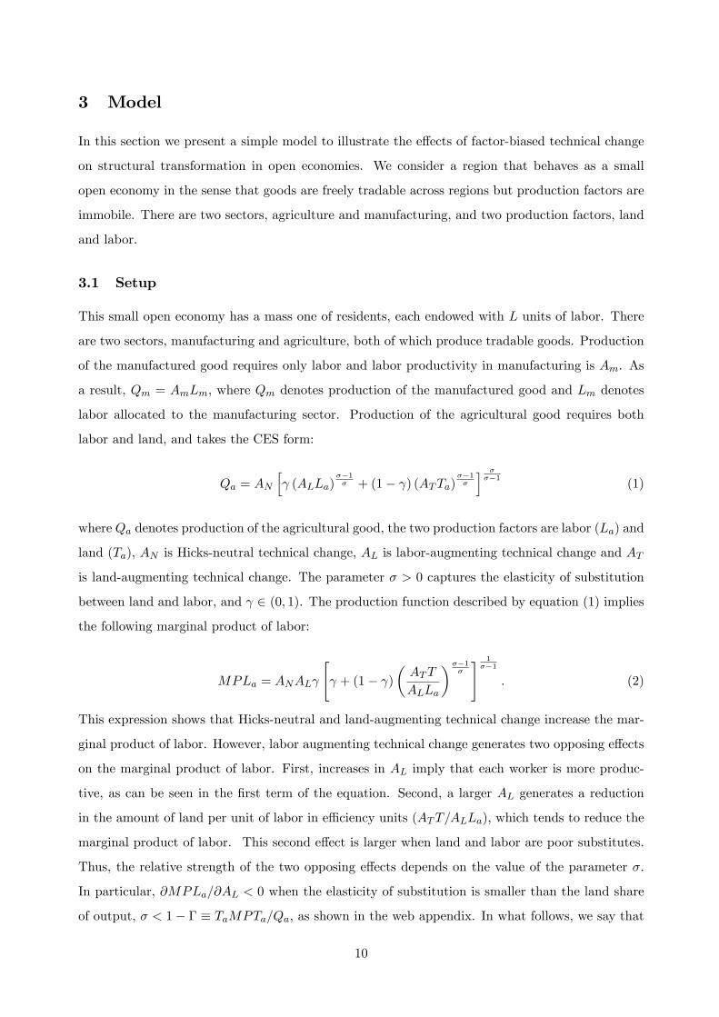
labor and land, and takes the CES form:
Qa = AN
[γ (ALLa)
σ−1σ + (1− γ) (ATTa)
σ−1σ
] σσ−1
(1)
where Qa denotes production of the agricultural good, the two production factors are labor (La) and
land (Ta), AN is Hicks-neutral technical change, AL is labor-augmenting technical change and AT
is land-augmenting technical change. The parameter σ > 0 captures the elasticity of substitution
between land and labor, and γ ∈ (0, 1). The production function described by equation (1) implies
the following marginal product of labor:
MPLa = ANALγ
[γ + (1− γ)
(ATT
ALLa
)σ−1σ
] 1σ−1
. (2)
This expression shows that Hicks-neutral and land-augmenting technical change increase the mar-
ginal product of labor. However, labor augmenting technical change generates two opposing effects
on the marginal product of labor. First, increases in AL imply that each worker is more produc-
tive, as can be seen in the first term of the equation. Second, a larger AL generates a reduction
in the amount of land per unit of labor in effi ciency units (ATT/ALLa), which tends to reduce the
marginal product of labor. This second effect is larger when land and labor are poor substitutes.
Thus, the relative strength of the two opposing effects depends on the value of the parameter σ.
In particular, ∂MPLa/∂AL < 0 when the elasticity of substitution is smaller than the land share
of output, σ < 1− Γ ≡ TaMPTa/Qa, as shown in the web appendix. In what follows, we say that
10

technical change is strongly labor-saving when this condition is satisfied.18 ,19
3.2 Equilibrium
We consider a small open economy that trades with a world economy where the relative price of
the agricultural good is Pa/Pm = (Pa/Pm)∗ . Profit maximization implies that the value of the
marginal product of labor must equal the wage in both sectors, thus:
PaMPLa = w = PmMPLm. (3)
As a result, in equilibrium, the marginal product of labor in agriculture is determined by interna-
tional prices and manufacturing productivity: MPLa = (Pm/Pa)∗Am. This condition and the land
market clearing condition (Ta = T ) determine the equilibrium allocation of labor:
L∗a =ATT
AL
{γ
1− γ1− Γ∗
Γ∗
} σ1−σ
, (4)
where the equilibrium labor share is Γ∗ = γσ (PmAm/PaANAL)1−σ . In turn, the equilibrium level
of employment in manufacturing, L∗m, can be obtained using the labor market clearing condition,
Lm + La = L. Once L∗m and L∗a are determined output in each sector can be found using the
production functions described in section 3.1. See Appendix for detailed derivations.
3.3 Technological Change and Structural Transformation
In this section we assess the response of agricultural and manufacturing employment to three types
of technological change: labor-augmenting, land-augmenting and Hicks-neutral.
Labor-augmenting technical change
The effect of labor augmenting technical change on agricultural employment depends on whether
the elasticity of substitution is smaller than the equilibrium land share of agricultural production
(σ < 1−Γ∗). When this condition is satisfied, we say that land and labor are strong complements.
a) Land and labor are strong complements: ∂L∗a∂AL
< 0 and ∂L∗m∂AL
> 0.
An increase in AL generates a reallocation of labor from agriculture to manufacturing.This is be-
cause if the elasticity of substitution between land and labor is smaller than the land share of
18Note that, because the production function takes the C.E.S. form, the land share of output is a function of theequilibrium level of employment in agriculture. In particular, in the relevant case where σ < 1 the land share isincreasing on the level of agricultural employment. As a result, this condition is more likely to be satisfied when theequilibrium level of agricultural employment is high.19See Neary (1981) and Acemoglu (2010) for more general discussions of the properties of technical change that
reduces the marginal product of labor. We follow Acemoglu in using the term strongly labor saving.
11
output, labor-augmenting technical change induces a reduction in the marginal product of labor
in agriculture. In equilibrium, the marginal product of labor in agriculture is given by interna-
tional prices and manufacturing productivity, thus it must stay constant when AL increases. Thus,
employment in agriculture must fall to increase the marginal product of labor to its equilibrium
level.
Proof. See Appendix.
b) Land and labor are not strong complements: ∂L∗a
∂AL> 0 and ∂L∗m
∂AL< 0.
An increase in AL generates a reallocation of labor from manufacturing to agriculture. This is
because if the elasticity of substitution is larger than the land share of output, labor-augmenting
technical change induces an increase in the marginal product of labor in agriculture.
Land-augmenting technical change: ∂L∗a
∂AT> 0 and ∂L∗m
∂AT< 0.
An increase in AT generates a reallocation of labor from manufacturing to agriculture. To see why
this is the case, note that land-augmenting technical change rises the marginal product of labor in
agriculture (see equation 2).
Hicks-neutral technical change: ∂L∗a
∂AN> 0 and ∂L∗m
∂AN< 0.
An increase in AN generates a reallocation of labor from manufacturing to agriculture. To see why
this is the case, note that a Hicks-neutral increase in agricultural productivity rises the marginal
product of labor in agriculture (see equation 2).
3.4 Empirical Predictions
In the following section, we test the predictions of the model by studying the simultaneous expansion
of two new agricultural technologies: GE soy and second-harvest maize. In the case of soy, the
advantage of GE seeds relative to traditional ones is that they are herbicide resistant, which reduces
the need to plow the land. As a result, this new technology requires less labor per unit of land
to yield the same output and can be characterized as labor-augmenting technical change. In the
case of maize, farmers started introducing advanced cultivation techniques and inputs which permit
to grow two crops a year, effectively increasing the land endowment. Thus, this new technology
can be characterized as land-augmenting technical change. In our empirical analysis, we quantify
the effects of these two types of technical change on observable variables in the agricultural and
manufacturing sector and test whether they display the sign patterns predicted by the model.
We analyze data aggregated at the municipality level, which is our unit of analysis. As a result,
we interpret the production functions in the model as describing the aggregate level of agricultural
12

and manufacturing production (Qa and Qm) in a given municipality. In addition, the agricultural
census reports information on employment aggregated across agricultural activities. Thus, we
interpret equation (1) as describing the aggregate production function for the agricultural sector,
where PaQa is the value of agricultural output, La is agricultural employment and Ta is land in
agricultural establishments. We trace the effects of the two new agricultural technologies on these
directly observed variables to test the following predictions of the model regarding the effects of
technical change.
Prediction 1. If land and labor are strong complements in production, labor augmenting technical
change in agriculture (AL) :
(a) increases the value of output per worker, P∗aQ∗a
L∗a;
(b) reduces the labor intensity of production, L∗aT ;
(c) reduces the employment share of agriculture, L∗aL ;
(d) increases the employment share of manufacturing,L∗mL .
Proof. See Appendix.
Prediction 2. Land augmenting technical change in agriculture (AT ) :
(a) does not change the value of output per worker;
(b) increases the labor intensity of production;
(c) increases the employment share of agriculture;
(d) reduces the employment share of manufacturing.
Proof. See Appendix.
3.5 Services
In this section we extend the model by including a third sector which produces non-traded services.
The purpose of this extension is to understand to what extent the predictions of the model discussed
above are modified by the presence of non-traded goods. A detailed analysis of the model with
services and all derivations are contained in the appendix.
We assume that the production function for services uses only labor and displays constant
returns to scale. As a result, Qs = AsLs, where Qs denotes production of services and Ls denotes
labor allocated to the service sector. Note that because services are non-tradable, production can
no longer be determined independently of consumption. Thus, we specify preferences and factor
ownership. Consumers have the following Cobb-Douglas preferences over the three goods:
U(ca, cm, cs) = cαaa cαmm cαss , (5)
13

where αa+αm+αs = 1.20 There are-two types of agents in the economy: L workers, each endowed
with one unit of labor; and T land-owners, each endowed with one unit of land. We assume that
workers reside in the same region where they work. In contrast, land owners can reside in any
region. We denote by θ the share of land owners residing in the same region where their land is
located. Then, aggregate service consumption in a region is Cs = cs,L L + cs,T θT, where cs,L is
the consumption of workers and cs,T the consumption of land-owners.21 ,22
In this setting, equilibrium employment in agriculture is the same as in the model without non-
traded services, given by equation (4). This is because wages are set by the value of the marginal
product of labor in manufacturing. Thus, the effects of agricultural technical change on agricultural
employment are identical to the ones in the model without services. We call them the supply-side
effects of technical change: ∂L∗a∂Ai
for i = N,T, L.
In turn, equilibrium employment in services can be written as:
L∗s = αsL+ αsθr∗
w∗T. (6)
where r∗ is the equilibrium land rent.23 Note that workers spend a constant share of their labor
endowment on services (αsL). This is because the service sector uses only labor for production.
Thus, any increase in wages has both an income and substitution effect on the demand for services
by workers. The income effect increases their demand for services as their labor endowment is more
valuable. The substitution effect reduces the demand for services as their price, the wage, increases.
When preferences are Cobb-Douglas both effects have the same magnitude and cancel-out.24 As a
result, agricultural technical change can only affect the demand for services through its effect on
the consumption of land owners: αsθ r∗
w∗T. In turn, agricultural technical change always increases
land rents. Thus, the demand for services and employment in the service sector increase. We call
20Our use of a homothetic utility function follows the findings in Herrendorf, Rogerson and Valentinyi (2013). Theyshow that a homothetic utility function where the elasticity of substitution across sectors is smaller than one providesthe best fit to the Postwar U.S. data when sectoral consumption data is measured in terms of value added. Becausewe use data on employment to measure structural transformation, our analysis tracks value added better than finalgoods consumption. As a result we use a homothetic utility function. However, we assume that the elasticity ofsubstitution across sectors is equal to one to make the model simpler. We discuss below how the predictions of ourmodel would be modified if this elasticity was smaller than one.21Note that θ is the share of services consumption of land owners that is spent locally. Thus, an alternative
interpretation is that land-owners reside locally but consume some services in other regions.22Note that we are not taking into account the local consumption of land owners who reside in the region under
consideration but own land in other regions. The reason for this omission is that, in the model, their demand forservices would not be affected by technical change in the region where they live but in the region where they ownland.23See appendix for detailed derivations and closed form solutions for r∗ and L∗s .24 If, instead of Cobb-Douglas, preferences were homothetic with an elasticity of substitution smaller than one, as
suggested by Herrendorf et al. (2013), the income effect would dominate. Thus, the demand for services from workerswould be increasing in wages.
14
this the demand side effects of technical change: ∂L∗s∂Ai
for i = N,T, L.
When technical change is Hicks-neutral or land-augmenting, both the supply-side and demand-
side effects reduce manufacturing employment. However, when technical change is strongly labor-
saving each effect moves manufacturing employment in opposite directions. On the one hand, the
supply side effect releases labor from agriculture, increasing the labor supply for manufacturing.
On the other hand, the demand-side effect increases labor demand in services, reducing the supply
of labor for manufacturing. Therefore, the net effect on manufacturing employment depends on the
relative strength of each effect. In the appendix, we show that the supply-side effect dominates as
long as σ < (1− Γ∗) (1− αsθ) . Note that because 1− αsθ < 1, this condition is stronger than the
condition required for agricultural technical change to be strongly labor-saving : σ < 1−Γ∗. Thus,
it is satisfied as long as land-owners’s consumption share of local services (αsθ) is not too large.
4 Data
The main data sources are the Agricultural Census, the Population Census, and the FAO Global
Agro-Ecological Zones database. To perform robustness checks we also use manufacturing plant-
level data from the Brazilian Annual Industrial Survey (PIA).25
The Agricultural Census is released at intervals of 10 years by the Instituto Brasileiro de Ge-
ografia e Estatística (IBGE), the Brazilian National Statistical Institute. The empirical analysis
focuses on the last two rounds of the census which have been carried out in 1996 and in 2006.
The Agricultural Census data is collected through direct interviews with the managers of each
agricultural establishment and is made available online by the IBGE aggregated at municipality
level.26 The agricultural variables of interest are the share of agricultural land planted with soy
and maize, the value of production per worker, and labor intensity.27 The last two variables are
aggregated across all agricultural activities. This is because the unit of observation in the census
is the agricultural establishment, and these tend to perform several activities. As a result, it is not
25 In this section we briefly discuss the main data sources and variables of interest. For detailed variable definitionsee Section A4 of the Appendix.26Borders of municipalities often change, thus, to make them comparable across time, IBGE has defined Área
Mínima Comparável (AMC), smallest comparable areas, which we use as our unit of observation. The average size ofan AMC in terms of population is 39,858 inhabitants, while the average size of a municipality is 30,833 inhabitants(data from the 2000 Population Census). In terms of area, the average AMC has an area of around 2,000 squarekilometers, while the average municipality has an area of 1,500 square kilometers.27The measure of agricultural employment used to construct the value of production per worker and labor intensity
includes: employees, family members employed in farm activities, sharecroppers and people who reside in the farm andperform agricultural activities without a formal contract. There are two potential problems with this definition. Thefirst is potential double counting of seasonal workers that work in more than one farm during the same calendar year.The second is that this variable does not include employees hired by service provider companies that are contractedby the farm to perform agricultural activities. See section A4 of the Appendix for a more detailed description of thisvariable.
15
possible to obtain a measure of employment by crop.
We use the Brazilian Population Census to construct measures of the sectoral composition
of employment and average wages. The Population Census is conducted every 10 years and it
covers the entire Brazilian population. We use data from the last two rounds of the census (2000
and 2010) so to observe the variables of interest before and after the legalization of the GE soy
seeds.28 Data on the sector of employment is collected through a special survey that is administered
to a representative sample of the Brazilian population within narrow cells defined by geographical
district, sex, age and urban or rural residence. The variables we focus on are the sector in which the
person was working during the previous week and its wage. 29 For each municipality, we compute
employment shares as the number of workers in each sector divided by total employment.30
We obtain an exogenous measure of technological change in agriculture by using estimates of
potential soy and maize yields across geographical areas of Brazil from the FAO-GAEZ database.
These yields are calculated by incorporating local soil and weather characteristics into a model
that predicts the maximum attainable yields for each crop in a given area. In addition, the data-
base reports potential yields under different technologies or input combinations. Yields under the
low technology are described as those obtained planting traditional seeds, no use of chemicals nor
mechanization. Yields under the high technology are obtained using improved high yielding vari-
eties, optimum application of fertilizers and herbicides and mechanization.31 Maps displaying the
resulting measures of potential yields for soy and maize under each technology are contained in
Appendix Figures A2 to A5.
We construct a measure of technical change in soy or maize production for each municipality by
deducting the average potential yield under low inputs from the average potential yield under high
inputs. Figure 2 illustrates the resulting measure of technical change in soy at the municipality
level, while Figure 3 shows the same measure at the micro-region level.
Finally, we use data from the Pesquisa Industrial Anual (PIA), the Annual Industrial Survey
conducted by the IBGE. We focus on firms operating in the manufacturing sector32 and use yearly
data from 1996 to 2007. All firms with more than 5 employees registered in the national firm registry
(CEMPRE, Cadastro Central de Empresas) are eligible for this survey. The survey is constructed
using two strata: the first includes a sample of firms having between 5 and 29 employees (estrato
28To perform some of the robustness checks we also use the 1980 and 1991 Population Censuses.29The sector classification is comparable across the census of 2000 and 2010 and it is the CNAE Domiciliar 1.0.
The broader categories of CNAE Domiciliar 1.0 follow the structure of the ISIC classification version 3.1.30We restrict the sample to workers aged between 16 and 55 years old.31See section A4 of the Appendix for a more detailed definition of potential yields under different input combina-
tions.32 Identified by the CNAE sector codes 15 to 37
16

amostrado) and it is representative at the sector and state level. The second includes all firms
having 30 or more employees (estrato certo). We construct measures of total employment and
average wages that are representative at municipality level by focusing on firms with 30 or more
employees.
5 Empirics
In this section we study the effects of the adoption of new agricultural technologies on structural
transformation in Brazil. For this purpose, we first study the effect of the adoption of GE soy and
second season maize on agricultural productivity and the factor intensity of agricultural production.
This first step permits to characterize the factor-bias of technical change. Next, we assess the impact
of technical change on the allocation of labor across sectors.
In the following section we report simple correlations between the expansion of the area planted
with soy and maize and agricultural and industrial labor market outcomes in each municipality.
As discussed above, these correlations are not informative about the causal relation between these
variables. Thus, in section 5.2, we present an empirical strategy that attempts to establish the
direction of causality by exploiting the timing of adoption and the differential impact of the new
technology on potential yields across geographical areas.
5.1 Basic Correlations in the Data
We start by documenting how the expansion of soy and maize cultivation during the 1996-2006
period relates to changes in agricultural production and industrial employment. These basic corre-
lations in the data attempt to answer the following question: did areas where soy (maize) expanded
experience faster (slower) structural transformation? In section 5.1.1 we present a set of OLS esti-
mates of equations relating agricultural outcomes to the percentage of farm land cultivated with soy
and maize. In the following section 5.1.2 we present the corresponding estimates for manufacturing
outcomes.
The basic form of the equations to be estimated in this section is:
yjt = αj + αt + β
(Soy Area
Agricultural Area
)jt
+ γ
(Maize Area
Agricultural Area
)jt
+ εjt (7)
where j indexes municipalities, t indexes time, αj are municipality fixed effects and αt are time
fixed effects. yjt is an outcome that varies across municipalities and time andSoy (Maize) AreaAgricultural Area is the
total area reaped with soy (maize) divided by total farm land.33 We observe agricultural outcomes33Total farm land includes areas devoted to crop cultivation (both permanent and seasonal crops), animal breeding
17

for the census years 1996 and 2006. Because fixed effects and first difference estimates are identical
when considering only two periods, we estimate (7) in first differences:
∆yj = ∆α+ β ∆
(Soy Area
Agricultural Area
)j
+ γ ∆
(Maize Area
Agricultural Area
)j
+ ∆εj (8)
5.1.1 Agricultural Outcomes: Productivity, Labor Intensity and Employment Share
Table 4 reports OLS estimates of equation (8) for three agricultural outcomes. The first is labor
productivity, measured as the value of output per worker in agriculture.The second is labor intensity,
measured as the number of workers per unit of land in agriculture. The third outcome is the
employment share of agriculture.
The first two columns of Table 4 show that in areas where soy cultivation expanded, the value
of agricultural production per worker increased and labor intensity in agriculture decreased. These
empirical findings are consistent with the characterization of soy technical change as strongly labor-
saving. The estimated coeffi cients imply that a 1 percentage point increase in soy area share
corresponds to a 0.58 percent increase in labor productivity, and a 0.48 percent reduction in labor
intensity. In contrast, in areas where maize cultivation expanded labor intensity increased. This
evidence is consistent with our characterization of technical change in maize as land-augmenting.
The estimated coeffi cients imply that a 1 percentage point increase in maize area share corresponds
to a 1.6 percent increase in labor productivity, and a 0.74 percent increase in labor intensity.
Next, we analyze the relationship between the expansion in soy and maize area and sectoral
employment shares. Note that we source information on sectoral employment shares from the
Population Census which reports information for the years 2000 and 2010. Thus, our estimation of
equation (8) relates changes in employment shares between 2000 and 2010 to changes in the area
planted with soy and maize between 1996 and 2006. In both cases the initial year precedes the
timing of legalization of soybean seeds in Brazil (2003), as well as the first date in which smuggling
of GE soy seeds was documented (2001). Column 3 of Table 4 shows that the employment share of
agriculture decreased in places where soy expanded while estimates for maize are not statistically
significant. The estimated coeffi cient implies that a 1 percentage point increase in soy area share
corresponds to a 0.09 percentage point reduction in the agricultural employment share.
The finding that the agricultural employment share fell in areas where soy expanded suggests
that soy technical change is not only labor-augmenting but also strongly labor-saving. In this case,
our model predicts that technology adoption reduces labor demand in agriculture.
and logging.
18
5.1.2 Manufacturing Outcomes: Employment Share, Total Employment and Wages
We now turn to the question of whether manufacturing employment expanded (contracted) in areas
where soy (maize) expanded. Table 5 reports OLS estimates of equation (8) for three manufacturing
sector outcomes: employment share, level of employment, and average wage.
The first column of Table 5 shows that municipalities where soy expanded experienced a faster
increase in the employment share in manufacturing. In contrast, this share remained unchanged
in municipalities where maize expanded. Interestingly, in areas where soy expanded, not only
the share but also the level of manufacturing employment increased, as shown in column 2. The
estimated coeffi cient on the effect of the expansion of soy cultivation in manufacturing employment
share indicates that municipalities experiencing a 1 percentage point increase in soy area share had
a 0.11 percentage point increase in manufacturing employment share and a 1.05 percent increase
in manufacturing employment.
5.2 The Effect of Agricultural Technological Change on Structural Transforma-
tion
In this section we provide empirical evidence on the causal effects of the adoption of new agricultural
technologies on industrial development in Brazil. The basic correlations in the data reported in
the previous section show that areas where soy expanded experienced an increase in output per
worker and a reduction in labor intensity in agriculture while industrial employment expanded.
These findings are consistent with the sequence of events predicted by the model, namely that the
adoption of strongly labor-saving agricultural technologies reduces labor demand in the agricultural
sector and induces a reallocation of labor towards the industrial sector. However, these correlations
are not informative about the direction of causality. For example, these correlations are consistent
with the following alternative sequence of events: productivity growth in the industrial sector
increases labor demand and wages, inducing agricultural firms to switch to less labor-intensive
crops, like soy. In this section we attempt to establish the direction of causality.
Our empirical strategy relies on the assumption that goods can be traded across geographical
areas of Brazil but labor markets are local. We investigate whether exogenous shocks to local
agricultural productivity lead to changes in the size of the local industrial sector. Thus, our ideal
unit of observation would be a region containing a city and its hinterland with limited migration
across regions. We attempt to approximate this ideal using municipalities as our main level of
geographical aggregation. This approach is adequate for municipalities in the interior of the country,
which typically include both rural and urban areas. However, municipalities tend to be mostly urban
19
in more densely populated coastal areas. To address this concern, we show that our estimates are
robust to using a larger unit of observation: micro-regions. Figures 2 and 3 contain maps of Brazil
displaying both levels of aggregation.34
We propose to identify the causal effect the new technologies on structural transformation by
exploiting the timing of adoption and the differential impact of the new technology on potential
yields across geographical areas. Let us first consider whether the timing of adoption is likely to be
exogenous with respect to developments in the Brazilian economy. GE soy seeds were commercially
released in the U.S. in 1996, and legalized in Brazil in 2003. Given that the seeds were developed
in the U.S., their date of approval for commercialization in the U.S., 1996, is arguably exogenous
with respect to developments in the Brazilian economy. In contrast, the date of legalization, 2003,
responded partly to pressure from Brazilian farmers. In addition, smuggling of GE soy seeds across
the border with Argentina is reported since 2001. Thus, in our empirical analysis we would ideally
compare outcomes before and after 1996. This is possible when variables are sourced from the
Agricultural Census. For variables sourced from the Population Census we compare outcomes before
and after 2000. Because this year predates both legalization and the first reports of smuggling, the
timing can still be considered exogenous.
Second, the new technology had a differential impact on potential yields depending on soil and
weather characteristics. Thus, we exploit these exogenous differences in potential yields across
geographical areas as our source of cross-sectional variation in the intensity of the treatment. To
implement this strategy, we need an exogenous measure of potential yields for soy, which we obtain
from the FAO-GAEZ database. These potential yields are estimated using an agricultural model
that predicts yields for each crop given climate and soil conditions. As potential yields are a func-
tion of weather and soil characteristics, not of actual yields in Brazil, they can be used as a source of
exogenous variation in agricultural productivity across geographical areas. Crucially for our analy-
sis, the database reports potential yields under different technologies or input combinations. Yields
under the low technology are described as those obtained using traditional seeds and no use of
chemicals, while yields under the high technology are obtained using improved seeds, optimum ap-
plication of fertilizers and herbicides and mechanization. Thus, the difference in yields between the
high and low technology captures the effect of moving from traditional agriculture to a technology
that uses improved seeds and optimum weed control, among other characteristics. We thus expect
this increase in yields to be a good predictor of the profitability of adopting herbicide-resistant GE
soy seeds.
34Micro-regions are groups of several municipalities created by the 1988 Brazilian Constitution and used for sta-tistical purposes by IBGE.
20
More formally, our basic empirical strategy consists in estimating the following equation:
yjt = αj + αt + β Asoyjt + εjt (9)
where yjt is an outcome that varies across municipalities and time, j indexes municipalities, t
indexes time, αj are municipality fixed effects, αt are time fixed effects and Asoyjt is equal to the
potential soy yield under high inputs from 2003 onwards and to the potential soy yield under low
inputs in the years before 2003. Asoyjt can be thought of as the empirical counterpart of the labor
augmenting technical change AL presented in our model.
In the case of agricultural outcomes, our period of interest spans the ten years between the
last two censuses which took place in 1996 and 2006. Similarly, in the case of sectoral employment
shares and manufacturing outcomes, our period of analysis spans the ten years between the last
two population censuses which took place in 2000 and 2010. We thus estimate a first-difference
version of equation (9):
∆yj = ∆α+ β∆Asoyj + δ Ruralj,1991 + ∆εjt (10)
where the outcome of interest, ∆yj is the change in outcome variables between the last two census
years; ∆Asoyj is the potential yield of soy under the high technology minus the potential yield of
soy under the low technology. Figure 2 contains a map of Brazilian municipalities displaying this
measure of technical change. Additionally, we include a control for the share of rural population in
1991 to allow for differential trends for municipalities with different initial urbanization rates. This
is important because, as mentioned above, coastal municipalities tend to have higher urbanization
rates and there were migration flows from rural to urban areas during the period under study.35
In the case of maize, we follow a similar empirical strategy. However, it is important to note that
the cultivation techniques necessary to introduce a second harvesting season were developed within
Brazil. Thus, the timing of its expansion can not be considered exogenous to other developments in
the Brazilian economy. Nevertheless, to the extent that the diffusion of this new technology across
space depends on exogenous local soil and weather characteristics, the variation in adoption which
we use in our empirical analysis is arguably exogenous to developments in the local industrial
sector. As noted in Section 2, the introduction of a second harvesting eason for maize requires
the use of modern techniques that are intensive in the use of fertilizers, herbicides and tractors.
Then, we expect that the the difference in FAO-GAEZ potential yields between the high and low
35The share of working age population residing in rural areas fell from 22% in 1991 to 14% in 2010.
21
technology captures the profitability of introducing a second harvesting season for maize. Thus,
we augment the equation described above to include the following variable: Amaizejt which is equal
to the potential maize yield under high inputs from 2003 onwards and to the potential maize yield
under low inputs in the years before 2003. Amaizejt can be thought of as the empirical counterpart
of the land augmenting technical change AT presented in our model:
∆yj = ∆α+ β∆Asoyj + γ∆Amaizej + δ Ruralj,1991 + ∆εj (11)
where ∆Amaizej is the potential yield of maize under high inputs minus the potential yield of maize
under low inputs.
A potential concern with our identification strategy is that, although the soil and weather char-
acteristics that drive the variation in ∆Asoyj and ∆Amaizej across geographical areas are exogenous,
they might be correlated with initial levels of development across Brazilian municipalities. For
example, to the extent that municipalities with heterogeneous initial levels of development experi-
ence different growth paths, our estimates could be capturing differential structural transformation
trends across municipalities. To assess the extent of this potential concern we first compare observ-
able characteristics of municipalities with high and low levels of our exogenous measure of technical
change in agriculture. Whenever significant differences emerge, we show that our estimates are
stable when we introduce controls for differential trends across municipalities with heterogeneous
initial characteristics.
Table 6 compares municipalities above and below the median change in potential soy yields
(∆Asoyj ) in terms of observable characteristics in 1991, before the introduction of GE soy.36 Mu-
nicipalities above the median potential increase in soy yields are characterized by smaller shares
of rural population and agricultural employment. In addition, they display a larger manufactur-
ing employment share, literacy rate, and income per capita than municipalities below the median.
Thus, in what follows, we always show that our estimates are stable when we introduce controls
for differential trends across municipalities with heterogeneous initial characteristics in our baseline
specification 11, as follows:
∆yj = ∆α+ β∆Asoyj + γ∆Amaizej + δ Ruralj,1991 + θXj,1991 + ∆εj (12)
where Xj,1991 are the set of municipality characteristics discussed above.
In the following subsections we report estimates of the effects of technical change on agricultural
36Municipalities below the median level of ∆Asoyjt experience, on average, a 1.06 tons per hectare increase inpotential soy yield, while those with above the median experience a 2.5 tons per hectare increase.
22
production and the sectoral composition of employment. In particular, we report estimates of
the effects of technical change on the expansion of soy and maize cultivation in section 5.2.1; on
agricultural outcomes in section 5.2.2; on manufacturing outcomes in section 5.2.3; and on services
in section 5.2.4.
5.2.1 Agricultural Outcomes: Soy and Maize Expansion
In this section we document the relationship between technical change measured by the increase in
the FAO-GAEZ potential yields of soy and maize, and the actual change in the share of agricultural
land cultivated with each crop. The objective of this exercise is to check whether the change in
potential yields is a good proxy of the profitability of adoption of the new agricultural technologies.
If this is the case, we expect the increase in potential yield of a given crop to predict the actual
expansion in the share of agricultural land cultivated with that crop between 1996 and 2006.
First, we expect that areas with a higher increase in potential soy yields when switching to
the high technology are those adopting genetically engineered soy on a larger scale. Thus, we
start by estimating equation (10) where the outcome of interest, ∆yj is the change in the share
of agricultural land devoted to GE soy between 1996 and 2006. Note that because this share was
zero everywhere in 1996, the change in the area share corresponds to its level in 2006. Estimates
are shown in column 1 of Table 7: the increase in potential soy yield predicts the expansion in GE
soy area as a share of agricultural area between 1996 and 2006. The point estimate remains stable
when controlling for initial municipality characteristics, as shown in column 2.
In columns 3 and 4 of Table 7 we perform a falsification test by looking at whether our measure
of technical change in soy explains the expansion in the area planted with non-GE soy. In this
case, the coeffi cients are negative and significant. This finding supports our claim that the change
in potential soy yield captures the benefits of adopting GE soy vis-à-vis traditional soy seeds.
Next, we jointly analyze the effects of technical change in soy and maize on the area planted
with each crop. For this purpose, we use the broader measure of planted area with soy instead
of GE soy.37 This permits to control for municipality fixed effects by focusing on changes in area
planted rather than levels. We start by estimating equation (12) where the outcome of interest,
∆yj is the change in share of agricultural land devoted to either soy or maize between 1996 and
2006. Estimates are reported in Table 8. First, note that while soy technical change has a positive
effect on the area planted with soy (column 1), it does not have a significant effect on the area
planted with maize (column 4). Similarly, maize technical change only has a positive effect on the
37 In the case of maize, we can only focus on the broader measure of area planted with maize as the publicly availableAgricultural Census data does not contain information on the season of planting of maize at the municipality level.
23
area planted with maize (columns 2 and 3). These findings suggest the change in potential yields
when switching to the high technology are good measures of crop-specific technical change in soy
and maize during this period. In addition, both estimates are stable when we add controls for
municipality characteristics. This finding suggests that the differential expansion of these crops
across municipalities is not driven by differential trends across municipalities with different initial
levels of development.
The size of the estimated coeffi cient on ∆Asoyj implies that a one standard deviation increase
in potential soy yield corresponds to an increase in the soy share of agricultural land of 0.26 of a
standard deviation. To understand the magnitude of our estimate, this is an increase of agricultural
land devoted to soy by 877 hectares in response to a 0.85 tons per hectare increase in potential
soy yield. The corresponding estimate for maize implies that a one standard deviation increase in
potential maize yield corresponds to a 0.08 of a standard deviation increase in the maize share of
agricultural land. This means that, in response to a 1.8 tons per hectare increase in potential maize
yield, agricultural land devoted to maize increases by 426 hectares.
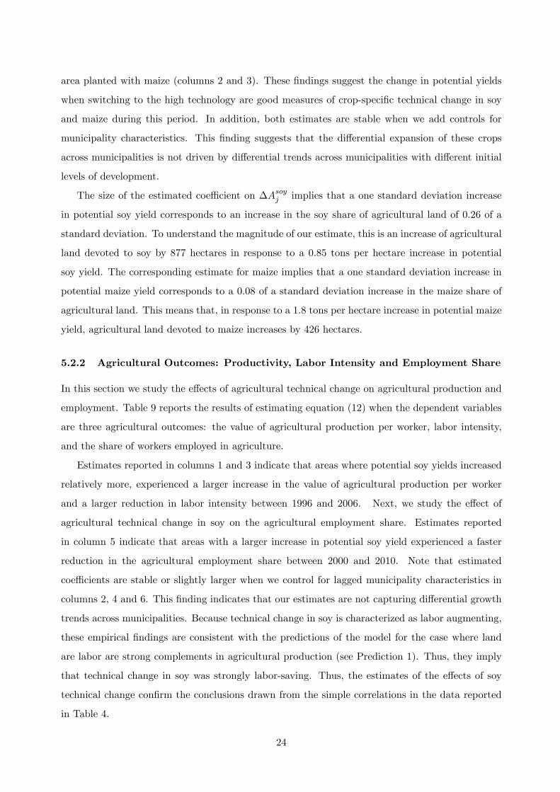
5.2.2 Agricultural Outcomes: Productivity, Labor Intensity and Employment Share
In this section we study the effects of agricultural technical change on agricultural production and
employment. Table 9 reports the results of estimating equation (12) when the dependent variables
are three agricultural outcomes: the value of agricultural production per worker, labor intensity,
and the share of workers employed in agriculture.
Estimates reported in columns 1 and 3 indicate that areas where potential soy yields increased
relatively more, experienced a larger increase in the value of agricultural production per worker
and a larger reduction in labor intensity between 1996 and 2006. Next, we study the effect of
agricultural technical change in soy on the agricultural employment share. Estimates reported
in column 5 indicate that areas with a larger increase in potential soy yield experienced a faster
reduction in the agricultural employment share between 2000 and 2010. Note that estimated
coeffi cients are stable or slightly larger when we control for lagged municipality characteristics in
columns 2, 4 and 6. This finding indicates that our estimates are not capturing differential growth
trends across municipalities. Because technical change in soy is characterized as labor augmenting,
these empirical findings are consistent with the predictions of the model for the case where land
are labor are strong complements in agricultural production (see Prediction 1). Thus, they imply
that technical change in soy was strongly labor-saving. Thus, the estimates of the effects of soy
technical change confirm the conclusions drawn from the simple correlations in the data reported
in Table 4.
24

The estimates discussed above can be used to compute the elasticity of the agricultural em-
ployment share to changes in agricultural labor productivity due to GE soy adoption. We compute
this elasticity as the ratio of the estimated coeffi cient on ∆Asoyj when the outcome is agricultural
employment share, and the estimated coeffi cient on ∆Asoyj when the outcome is agricultural labor
productivity.38 Using our more conservative estimates, namely those that include all municipality
controls in columns 2 and 6, this ratio is equal to: −0.021/0.131 = −0.158.39 The size of this
elasticity implies that a 1 percent increase in agricultural labor productivity corresponds to a 0.158
percentage points decrease in the agricultural employment share. To illustrate the magnitude of
these estimates, we compute how much of the differences in the speed of structural transformation
across Brazilian regions can soy technical change explain, as follows. Note that a municipality
shocked with a one standard deviation increase in potential soy yield experienced an increase in
agricultural labor productivity of 11 percent, and a corresponding 1.76 percentage points decrease
in agricultural employment share.40 This estimate corresponds to 24 percent of a standard devi-
ation in the change of the agricultural employment share between 2000 and 2010 (7.4 percentage
points, see Table 3).
In the case of maize, the estimated coeffi cients reported in columns 3 and 5 indicate that areas
with higher increase in potential maize yield experienced a larger increase in labor intensity and the
agricultural employment share during the period under study. These findings are consistent with
the predictions of the model for the effects of land-augmenting technical change (See Prediction 2).
In addition, column 1 shows that areas where maize yields increased relatively more experienced
a smaller increase in the value of agricultural output per worker. Our model is too stylized to
capture this feature in the data, which is likely driven by the across-crop effect of technical change:
reallocation of labor towards maize production reduces the value of output per worker in agriculture.
This is because maize production is more labor-intensive than soy production, thus the value of the
average product of labor is lower for maize.41
38Due to the different timing of the Agricultural and Population Censuses, agricultural labor productivity changesare measured over the period 1996-2006 while employment share changes are measured over the period 2000-2010.Thus, the elasticity estimates correspond to the effect of 4-year lagged agricultural productivity changes on employ-ment shares.39We compute this elasticity in the same way we would compute a Wald estimator in an instrumental variable
setting, where the estimated coeffi cient on ∆Asoyj in column 2 is the first stage coeffi cient, and the estimated coeffi cienton ∆Asoyj in column 6 is the reduced form coeffi cient.40The first number is computed multiplying one standard deviation in ∆Asoyj by the estimated coeffi cient on ∆Asoyj
in our specification with municipality controls when the outcome is agricultural labor productivity (column 2 of Table9): 0.851 × 0.131 = 0.111. The second number is computed multiplying the predicted increase in agricultural laborproductivity for one standard deviation in ∆Asoyj by the elasticity of agricultural employment share to agriculturallabor productivity: 0.111×−0.158 = −0.0176.41A more formal explanation of the effect of labor reallocation towards maize on the value of agricultural output
per worker follows. Suppose that there are only two crops, soy and maize, and two production factors, land andlabor. In addition, maize production is more labor-intensive than soy. The value of output per worker in agricultureis defined as PY
L≡ PmYm+PsYs
L= PmYm
Lm
LmL
+ PsYsLs
LsL. In this case, a reallocation of labor towards maize production
25

To sum up, the results presented in Table 9 suggest that the introduction of new agricultural
technologies in Brazil had a sizable impact on agricultural labor markets. Areas where the potential
impact of GE soy adoption was higher experienced an increase in the value of agricultural production
per worker, a reduction in the number of workers per unit of land, and a reduction in the employment
share of agriculture. These findings are consistent with the predictions of the model for the effects
of strongly labor-saving technical change. In the case of maize, areas where the potential impact of
the introduction of a second harvesting season was higher experienced an increase in labor intensity
and in the employment share of agriculture. These findings are consistent with the predictions of
the model for the effects of land-augmenting technical change.
5.2.3 Manufacturing Outcomes: Employment Share, Employment and Wages
In this section we study the effect of agricultural technical change on manufacturing employment
and wages. Table 10 reports the results of estimating equation (12) where the dependent variables
are three manufacturing outcomes: the employment share of manufacturing, the level of manufac-
turing employment, and the average wage in manufacturing.
The estimates indicate that areas where potential soy yields increased relatively more, ex-
perienced a larger increase in the manufacturing employment share between 2000 and 2010. A
comparison of point estimates reported in the first row of columns 1 and 2 shows that estimates
are stable when introducing controls for lagged municipality characteristics. In addition, columns
3 and 4 show that not only the share of manufacturing employment increased but also its absolute
level. Finally, columns 5 and 6 show that manufacturing wages fell. These estimates are consistent
with the empirical predictions of the model: technical change in soy is strongly labor-saving thus
reduces labor demand in agriculture, and induces an expansion of the manufacturing sector through
an increase in labor supply and lower wages.
The estimates discussed above can be used to compute the elasticity of manufacturing employ-
ment share to changes in agricultural labor productivity due to GE soy adoption. We compute
this elasticity as in section 5.2.2: we divide the estimated coeffi cient on ∆Asoyj when the outcome
is manufacturing employment share by the estimated coeffi cient on ∆Asoyj when the outcome is
agricultural labor productivity. When we estimate the specification including controls for lagged
municipality characteristics, this ratio is equal to: 0.021/0.131 = 0.161. This elasticity implies that
reduces the value of output per worker in agriculture. This is because if soy production is more land-intensive thanmaize production ( Ts
Ls> Tm
Lm), the value of the average product of labor is higher for soy (PsYs
Ls> PmYm
Lm). To see
why this is the case, note that the zero profit conditions for maize and soy (PiYi = rTi + wLi for i = s,m) implyPiYiLi
= r TiLi
+ w.
26

a 1% increase in agricultural labor productivity corresponds to a 0.161 percentage points increase
in manufacturing employment share. As in the previous section, we illustrate the magnitude of
these estimates by computing how much of the differences in the speed of structural transformation
across Brazilian regions can be explained by technical change in soy. Recall that a municipality
shocked with a one standard deviation increase in potential soy yield experienced an increase in
agricultural labor productivity of 11 percent,42 and a corresponding 1.79 percentage points increase
in manufacturing employment share.43 This estimate corresponds to 31% of a standard deviation
in the change of manufacturing employment share between 2000 and 2010 (5.7 percentage points,
see Table 3).
In the case of maize, the estimates reported in columns 1 and 2 of Table 10 indicate that
areas where potential maize yields increased relatively more experienced a smaller increases in the
manufacturing employment share. In addition, columns 3 and 4 show that not only the share of
manufacturing employment fell but also its absolute level. Finally, columns 5 and 6 show that
manufacturing wages increased. These estimates are consistent with prediction 2 of the model.
These estimates are consistent with the empirical predictions of our model: technical change in
maize is labor-biased thus increases labor demand in agriculture, generating an increase in wages
and a reallocation of labor away from the manufacturing sector.
5.2.4 Services and Other Sectors
In this section we complement our empirical findings with an analysis of the service sector. First,
note that the estimates of the effects of technical change on the agricultural and manufacturing
employment shares discussed above have a similar magnitude. To make this point clearer, we
reproduce them in Table 11, where we also include estimates for the service and other sectors.44
The point estimates of the effect of soy technical change on the agriculture and manufacturing
employment shares have the same size: they are -0.021 and 0.021, respectively, both with a standard
error of 0.002. At the same time, the estimates of the effects on the service and other sectors are very
small and not statistically different from zero. This implies that labor reallocated from agriculture
to manufacturing and not towards services.
42This number is computed as before, by multiplying one standard deviation in ∆Asoyj by the estimated coeffi cienton ∆Asoyj in our specification with municipality controls when the outcome is agricultural labor productivity (column2 of Table 9): 0.851× 0.131 = 0.11143This number is computed multiplying the predicted increase in agricultural labor productivity for one standard
deviation in ∆Asoyj by the elasticity of manufacturing employment share to agricultural labor productivity: 0.111×0.161 = −0.0179.44The services sector includes: construction, commerce, lodging and restaurants, transport, finance, housing ser-
vices, domestic workers and other personal services. Other sectors include: public administration, education, health,international organizations, extraction and public utilities.
27

In the theory section we identified two effects of labor-saving technical change in agriculture:
the supply effect and the demand effect. The supply effect is generated by the reduction in the
marginal product of labor in the agricultural sector, which reduces agricultural employment. The
demand effect is generated by the higher income resulting from agricultural productivity growth
which leads to increased demand for services. As a result, the net effect of agricultural technical
change on industrialization depends on the relative strength of the supply and demand effects.
In addition, the demand effect is driven by the increase land rents, thus its strength depends on
the extent to which land-owners consume services in the region where their land is located. This
suggests that the absence of an effect of technical change on employment in the service sector might
be related to the fact that in some areas of Brazil land owners do not reside locally or consume
services produced in large cities.
In sum, our empirical analysis implies that in regions more affected by agricultural technical
change labor reallocated from agriculture to manufacturing and not towards services. Our inter-
pretation of these findings is that the differences-in-differences empirical strategy is well suited to
identify the supply effect to the extent that labor markets are local. However, our model suggests
that it might not be suitable to identify the demand effect if land owners do not consume local
services. Thus, a further investigation of the effect of agricultural technical change on non-traded
sectors is left for future work.
5.3 Variable Factor Endowments
The model presented in Section 3 describes a small open economy where goods can be freely traded
but factor endowments are fixed. Our empirical strategy thus relies on the assumption that each
unit of observation behaves as a small open economy: goods can be traded across municipalities
but labor markets are local and there is a fixed supply of land. However, the period under study is
characterized by significant internal migration flows: 16 percent of the population aged between 16
and 55 years old had moved to their 2010 municipality of residence during the previous 10 years. In
addition, Brazil has vast areas of underutilized land, which were in part converted to agricultural
activities during the period under study. Between 1996 and 2006 the land used for cultivation or
cattle ranching increased by 7 percent to 154 million hectares in the regions of the North, North-
East and Center-West. Thus, in this section, we investigate the role of migration and the expansion
in the agricultural frontier.
28
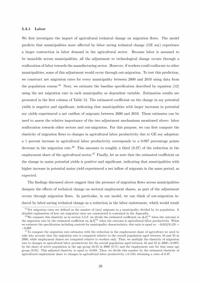
5.3.1 Labor
We first investigate the impact of agricultural technical change on migration flows. The model
predicts that municipalities more affected by labor saving technical change (GE soy) experience
a larger contraction in labor demand in the agricultural sector. Because labor is assumed to
be immobile across municipalities, all the adjustment to technological change occurs through a
reallocation of labor towards the manufacturing sector. However, if workers could reallocate to other
municipalities, some of this adjustment would occur through out-migration. To test this prediction,
we construct net migration rates for every municipality between 2000 and 2010 using data from
the population census.45 Next, we estimate the baseline specification described by equation (12)
using the net migration rate in each municipality as dependent variable. Estimation results are
presented in the first column of Table 12. The estimated coeffi cient on the change in soy potential
yields is negative and significant, indicating that municipalities with larger increases in potential
soy yields experienced a net outflow of migrants between 2000 and 2010. These estimates can be
used to assess the relative importance of the two adjustment mechanisms mentioned above: labor
reallocation towards other sectors and out-migration. For this purpose, we can first compute the
elasticity of migration flows to changes in agricultural labor productivity due to GE soy adoption:
a 1 percent increase in agricultural labor productivity corresponds to a 0.097 percentage points
decrease in the migration rate.46 This amounts to roughly a third (0.37) of the reduction in the
employment share of the agricultural sector.47 Finally, let us note that the estimated coeffi cient on
the change in maize potential yields is positive and significant, indicating that municipalities with
higher increase in potential maize yield experienced a net inflow of migrants in the same period, as
expected.
The findings discussed above suggest that the presence of migration flows across municipalities
dampen the effects of technical change on sectoral employment shares, as part of the adjustment
occurs through migration flows. In particular, in our model, we can think of out-migration in-
duced by labor-saving technical change as a reduction in the labor endowment, which would result
45Net migration rates are defined as the number of (net) migrants in a municipality divided by its population. Adetailed explanation of how net migration rates are constructed is contained in the Appendix.46We compute this elasticity as in section 5.2.2: we divide the estimated coeffi cient on ∆Asoyj when the outcome is
the migration rate by the estimated coeffi cient on ∆Asoyj when the outcome is agricultural labor productivity. Whenwe estimate the specification including controls for municipality characteristics, this ratio is equal to: −0.013/0.131 =−0.097.47To compare the migration rate estimates with the reduction in the employment share of agriculture we need to
take into account that the migration rate is computed relative to the overall population aged between 16 and 55 in2000, while employment shares are computed relative to workers only. Thus, we multiply the elasticity of migrationrate to changes in agricultural labor productivity for the overall population aged between 16 and 55 in 2000 (-0.097)by the share of active population in the age group 16-55 in 2000 (0.71) and the employment rate for that same agegroup (0.85). This adjusted elasticity is equal to -0.059. Then, we divide this number by the estimated elasticity ofagricultural employment share to changes in agricultural labor productivity (-0.158) obtaining a ratio of 0.37.
29

in a reduction in the manufacturing employment share. This is because equilibrium agricultural
employment is unaffected by a change in the labor endowment (see equation 4). In turn, the equi-
librium level of employment in manufacturing is determined by the labor market clearing condition,
Lm = L − L∗a. Thus, the manufacturing employment share must fall when the labor endowment
falls. As a result, the presence of migration dampens the positive effects of soy technical change on
the manufacturing employment share. A similar argument implies that the in-migration induced
by land augmenting technical change in maize would increase the manufacturing employment share
and dampen the effects of maize technical change.
5.3.2 Land
In this section we study the role of the expansion in the agricultural frontier. During this period
the frontier expanded not only over the Amazon rainforest but also in the Cerrado. This is a
tropical savanna eco-region in central Brazil where soils used to be too acidic and nutrient poor.
Starting from the 1980s these soils were treated by the Brazilian Agricultural Research Corporation,
EMBRAPA, which enabled agricultural activities to expand over these areas. The incorporation
if forest or fallow land into agricultural activities can potentially affect our estimates of the effects
of technical change. In the model, an expansion in the land endowment would have the same
effects as land augmenting technical change. Thus, differential increases in the land endowment
across regions could account for our finding that areas more affected by technical change in maize
experienced an increase in the agricultural employment share or attenuate our findings for the
effects of soy technical change.
To assess the extent to which our estimates are affected by expansions in the agricultural frontier
we test the predictions of the model in a subsample of municipalities where the land endowment did
not increase. In particular, we define frontier municipalities as those which experienced an increase
in land use for agricultural activities between 1996 and 2006 and split the sample of municipalities
in two groups: frontier and non-frontier (see map in Figure A6 in the Appendix). Next, we estimate
our baseline specification described by equation (12) separately for each subsample. Our estimates
of the effect of soy technical change on the agricultural and manufacturing employment shares in
the subsample of non-frontier (frontier) municipalities are only slightly larger (smaller) in absolute
value than estimates using the full sample, as shown in Columns 4 to 7 of Table 12. This finding
suggests that the expansion of the agricultural frontier does not significantly mitigate our baseline
estimates. In the case of maize, estimates of the effect of technical change on the agricultural and
manufacturing employment shares in the subsample of non-frontier municipalities are slightly larger
in absolute value than estimates using the full sample. In contrast, estimates are smaller and not
30
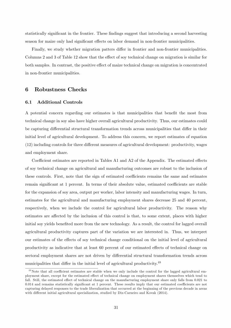
statistically significant in the frontier. These findings suggest that introducing a second harvesting
season for maize only had significant effects on labor demand in non-frontier municipalities.
Finally, we study whether migration patters differ in frontier and non-frontier municipalities.
Columns 2 and 3 of Table 12 show that the effect of soy technical change on migration is similar for
both samples. In contrast, the positive effect of maize technical change on migration is concentrated
in non-frontier municipalities.
6 Robustness Checks
6.1 Additional Controls
A potential concern regarding our estimates is that municipalities that benefit the most from
technical change in soy also have higher overall agricultural productivity. Thus, our estimates could
be capturing differential structural transformation trends across municipalities that differ in their
initial level of agricultural development. To address this concern, we report estimates of equation
(12) including controls for three different measures of agricultural development: productivity, wages
and employment share.
Coeffi cient estimates are reported in Tables A1 and A2 of the Appendix. The estimated effects
of soy technical change on agricultural and manufacturing outcomes are robust to the inclusion of
these controls. First, note that the sign of estimated coeffi cients remains the same and estimates
remain significant at 1 percent. In terms of their absolute value, estimated coeffi cients are stable
for the expansion of soy area, output per worker, labor intensity and manufacturing wages. In turn,
estimates for the agricultural and manufacturing employment shares decrease 25 and 40 percent,
respectively, when we include the control for agricultural labor productivity. The reason why
estimates are affected by the inclusion of this control is that, to some extent, places with higher
initial soy yields benefited more from the new technology. As a result, the control for lagged overall
agricultural productivity captures part of the variation we are interested in. Thus, we interpret
our estimates of the effects of soy technical change conditional on the initial level of agricultural
productivity as indicative that at least 60 percent of our estimated effects of technical change on
sectoral employment shares are not driven by differential structural transformation trends across
municipalities that differ in the initial level of agricultural productivity.48
48Note that all coeffi cient estimates are stable when we only include the control for the lagged agricultural em-ployment share, except for the estimated effect of technical change on employment shares themselves which tend tofall. Still, the estimated effect of technical change on the manufacturing employment share only falls from 0.021 to0.014 and remains statistically significant at 1 percent. These results imply that our estimated coeffi cients are notcapturing delayed responses to the trade liberalization that occurred at the beginning of the previous decade in areaswith different initial agricultural specialization, studied by Dix-Carneiro and Kovak (2014).
31
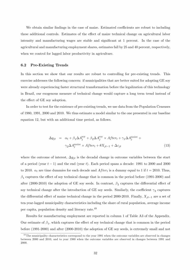
We obtain similar findings in the case of maize. Estimated coeffi cients are robust to including
these additional controls. Estimates of the effect of maize technical change on agricultural labor
intensity and manufacturing wages are stable and significant at 1 percent. In the case of the
agricultural and manufacturing employment shares, estimates fall by 25 and 40 percent, respectively,
when we control for lagged labor productivity in agriculture.
6.2 Pre-Existing Trends
In this section we show that our results are robust to controlling for pre-existing trends. This
exercise addresses the following concern: if municipalities that are better suited for adopting GE soy
were already experiencing faster structural transformation before the legalization of this technology
in Brazil, our exogenous measure of technical change would capture a long term trend instead of
the effect of GE soy adoption.
In order to test for the existence of pre-existing trends, we use data from the Population Censuses
of 1980, 1991, 2000 and 2010. We thus estimate a model similar to the one presented in our baseline
equation 12, but with an additional time period, as follows.
∆yjt = αt + β1∆Asoyj + β2∆A
soyj ×Aftert + γ1∆A
maizej +
γ2∆Amaizej ×Aftert + θXjt−1 + ∆εjt (13)
where the outcome of interest, ∆yjt is the decadal change in outcome variables between the start
of a period (year t− 1) and the end (year t). Each period spans a decade: 1991 to 2000 and 2000
to 2010. αt are time dummies for each decade and Aftert is a dummy equal to 1 if t = 2010. Thus,
β1 captures the effect of soy technical change that is common in the period before (1991-2000) and
after (2000-2010) the adoption of GE soy seeds. In contrast, β2 captures the differential effect of
soy technical change after the introduction of GE soy seeds. Similarly, the coeffi cient γ2 captures
the differential effect of maize technical change in the period 2000-2010. Finally, Xjt−1 are a set of
ten-year-lagged municipality characteristics including the share of rural population, average income
per capita, population density and literacy rate.49
Results for manufacturing employment are reported in column 1 of Table A3 of the Appendix.
Our estimate of β1, which captures the effect of soy technical change that is common in the period
before (1991-2000) and after (2000-2010) the adoption of GE soy seeds, is extremely small and not
49The municipality characteristics correspond to the year 1991 when the outcome variables are observed in changesbetween 2000 and 2010, and to year 1980 when the outcome variables are observed in changes between 1991 and2000.
32
statistically different from zero. This finding indicates that there are no pre-trends in manufac-
turing employment. In addition, our estimate of β2, which estimates the differential effect of soy
technical change on manufacturing employment after the introduction of GE soy seeds, is positive
and precisely estimated. Similarly, in the case of maize, we do not find pre-existing trends in man-
ufacturing employment. Note that we perform this test for the level of manufacturing employment
but not for the manufacturing and agricultural employment shares. This is because there were
important changes in the definition of employment after the 1991 Census, thus employment shares
can not be measured in a consistent way across the 1991 and 2000 Censuses.50
Column 2 of Table A3 shows the results of estimating equation (13) when the outcome variable
is the average wage in manufacturing. In this case, ∆Asoy had an opposite effect on manufacturing
wages between 1991 and 2000 with respect to the 2000-2010 period. Therefore, the existence of
these pre-existing trends in manufacturing wages attenuates our baseline estimated effects of soy
and maize technical change on wages in the period 2000-2010, presented in Table 10.
Finally, we check for pre-existing trends in migration. A potential concern is that areas that
are better suited for adopting GE soy experienced a pattern of migration prior to the legalization
of GE soy that affected farmers’incentive to adopt this new technology. For example, if these areas
experienced large out-migration in the decade before GE soy was legalized, farmers would have
had a higher incentive to adopt a labor-saving technology to cope with labor scarcity. Column 3 of
Table A3 shows the results of estimating equation (13) when the outcome variable is net migration
rate. The coeffi cient on ∆Asoy shows that there are no differential pre-existing trends in migration
for areas that have a higher increase in potential soy yields. Similarly, in the case of maize, we do
not find pre-existing trends in migration.51
These tests validate our interpretation that our estimates of the effects of agricultural technical
change on structural transformation are due to the introduction of new agricultural technologies50Between the 1991 and 2000 Censuses the Brazilian Statistical Institute (IBGE) changed its definition of employ-
ment in two important ways. First, it started to count zero-income workers as employed. In order to homogenize theBrazilian Census with international practices, the IBGE started to consider employed anyone who helped anotherhousehold member with no formal compensation, as well as agricultural workers that produced only for their ownconsumption (IBGE, 2003; p. 218). Zero-income workers are more common in agriculture than in other sectors, andin 1991 were only partially included in the labor force. In the 1991 Census 15% of agricultural workers reportedzero income, against 34% in 2000 and 35% in 2010. Second, the IBGE changed the reference period for consideringa person employed: while in 1991 such period included the last 12 months, in 2000 it only included the referenceweek of the Census. This new rule implied that workers performing temporary and seasonal activities that were notemployed during the reference week were counted in the 1991 census but not the in the 2000 census. This secondchange is likely to be especially problematic for the agricultural sector, considering that the reference week in the2000 Census was in the middle of the Brazilian winter. This is why, to test for pre-existing trends, we focus on theabsolute number of workers employed in manufacturing as an outcome (instead of its share in total employment).This measure is less likely to be affected by the changes introduced between the two censuses because: there arevery few zero-income workers in manufacturing (0.5%, 1.9% and 1% of manufacturing workers declare zero incomein 1991, 2000 and 2010, respectively); and manufacturing is less seasonal than other activities.51These results suggest that the migration flows generated by the expansion of the Brazilian road network in the
years 1960-2000 that are studied by Morten and Oliveira (2014) are unlikely to be confounding our results.
33

rather than to pre-existing trends in areas that were more affected by these new technologies.
6.3 Larger Unit of Observation: Micro-Regions
In the empirical analysis performed so far we assumed that municipalities are a good approximation
of the relevant labor market faced by Brazilian agricultural workers. A potential issue is that
local labor market boundaries do not overlap with a municipality’s administrative boundaries.
In particular, some municipalities might be too small to properly capture labor flows between
urban and rural areas, provided that manufacturing activities mostly take place in the former, and
agricultural activities in the latter. In order to take into account this concern we aggregate our data
at a larger unit of observation: micro-regions. These regions are groups of territorially contiguous
municipalities created, for statistical purposes, by the Brazilian Statistical Institute (IBGE). Table
13 reports the results of estimating equation (12) using micro-regions as a unit of observation. The
outcome variables are the same as in Table 10: change in manufacturing employment share, change
in manufacturing employment (in logs) and change in average manufacturing wage (in logs). The
estimates are consistent and similar in magnitude to those reported in Table 10, both for soy and
maize.
6.4 Input-Output Linkages
Our theoretical model predicts that agricultural technical change can have an effect on manufac-
turing employment through labor market forces. In the case of soy, for example, the adoption
of new agricultural technologies releases agricultural workers that find employment in the manu-
facturing sector. In this section we investigate to which extent our findings reflect the strength of
another channel through which agricultural technical change can affect manufacturing employment:
input-output linkages. Soy and maize farming require inputs produced by other sectors, including
manufacturing. Therefore, for example, an expansion of the area farmed with soy in a given mu-
nicipality might drive an increase in manufacturing employment in industries that produce inputs
used in soy production, such as chemicals or fertilizers. To the extent that manufacturing firms
producing chemicals and fertilizers used in agriculture face high transport costs, there might be an
incentive for them to locate in the same municipality in which agricultural production takes place.
Therefore, the effect of agricultural technical change on manufacturing that we show in Table 10
could be explained by an increase in the agricultural demand for manufacturing inputs. A similar
argument applies for manufacturing industries that use soy and maize as intermediate inputs, such
as the food processing industry. In order to assess the contribution of these direct linkages on our
34
estimates, we construct a measure of manufacturing employment that excludes the sectors directly
linked to soy and maize production through input-output chains.
In order to identify input-output linkages in the data, we proceed as follows. We use the
Brazilian input-output matrix (IBGE, 2008) to identify manufacturing sectors that are providing
inputs, or receiving outputs, from the soy and maize sectors. On the input side, soy and maize are
used as intermediate goods in only one manufacturing sector: the food and beverage sector, which in
2005 purchased around half of the total Brazilian production of both crops. On the output side the
matrix is less detailed, thus we use information on goods purchased by agricultural and breeding
farms in general. Half of the inputs purchased by these farms are supplied by manufacturing
sectors and four commodities account for 84% of the total value of inputs purchased: inorganic
chemicals, fertilizers, diesel oil and maize oil. These commodities are produced by the chemical
industry, the oil refining industry and the food and beverage industry. We use this information to
construct measures of employment and wages in manufacturing that exclude those industries that
are providing inputs, or receiving outputs, from the soy and maize sectors.
Table 14 reports estimates of our baseline specification described by equation (12) using as
outcome variables measures of manufacturing employment and wages that exclude workers em-
ployed in sectors directly linked to soy and maize. Estimates of the effect of soy technical change
on the manufacturing employment share and level are positive, precisely estimated and 38 to 10
percent smaller than our baseline estimates displayed in Table 10.52 In turn, the effect of technical
change in soy on manufacturing wages decreases substantially, and is not precisely estimated. In the
case of maize, estimated coeffi cients are essentially unaffected by excluding workers in downstream
and upstream manufacturing sectors when the outcomes are manufacturing employment share and
level. As in the case of soy, the effect on manufacturing wages decreases in size and is not precisely
estimated. Taken together, the results presented in this section imply that at least 62 percent of
our estimated effect of agricultural technical change on the manufacturing employment share is not
driven by the processing of soy and maize in downstream industries nor larger agricultural sector
demand for manufacturing inputs. A more detailed analysis is needed to separate the role of labor
market and input-output forces in the remaining 38 percent of the total estimated effect, which is
an interesting avenue for further work.
52 In our specification with all initial municipality controls, the point estimate on ∆Asoy when the outcome ismanufacturing employment share goes from 0.021 to 0.013. We can reject the null hypothesis that these two coeffi cientsare equal. When the outcome is manufacturing employment instead, the point estimate on ∆Asoy goes from 0.186to 0.167. In this case, the two coeffi cients are not statistically different.
35
6.5 Commodity Prices
In this section we show that our results are robust to controlling for international commodity prices.
To the extent that variation in international prices of soy and maize affect agricultural outcomes
in all Brazilian municipalities proportionally, their effects are captured by the time fixed effects
in equation (9). However, price changes might have heterogeneous effects across municipalities
with different suitability to the cultivation of soy and maize. For example, an increase in the
international price of soy could induce farmers to expand the area devoted to soy relatively more
in municipalities that are initially more suitable for its cultivation.
Figures A7 and A8 display the evolution of international prices of soy and maize, expressed in
2000 US$. These Figures show how the international prices of both commodities have been in an
upward trend starting from year 2007. This pattern most likely does not affect our estimates when
we use data for the last two Agricultural Censuses: 1996 and 2006. In particular, note that the
international price for both soy and maize was lower in 2006 than in 1996. However, when we use
data from the last two Population Censuses, which took place in 2000 and 2010, the end of period
year is characterized by high international soy and maize prices with respect to the initial year.
To address this concern, we assess the robustness of our findings for the manufacturing sector to
controlling for changes in commodity prices.
The data from the Population Censuses does not allow us to control for yearly variation in soy
and maize prices. We therefore rely on an alternative source of data for manufacturing outcomes:
the Annual Manufacturing Survey (PIA). The Annual Manufacturing Survey is carried out yearly,
allowing us to both exclude years of high international commodity prices and fully control for price
variation. It covers the universe of manufacturing firms with at least 30 employees in Brazil, and
it is therefore representative at municipality level for this class of firms. We focus on two variables
from this survey: manufacturing employment and average wages.53
We estimate an equation of the following form:
yjt = αj + αt + βAsoyjt + γAmaizejt +∑z
γzPzt A
zj0 + δRuralj1991 × t+ θXjt1991 × t+ εjt (14)
where yjt is total employment or average wage in a given municipality; Asoyjt is equal to the potential
soy yield under low inputs for all years before 2003 and to the potential soy yield under high inputs
starting from 2003 (same criteria is used to define Amaizejt ). We control for the prices of soy and maize
53The average wage is defined as the aggregate wage bill (in real terms) divided by the total number of workersemployed in a municipality.
36

by multiplying the potential yield under low inputs of each crop by the time varying international
price of each crop. Finally, we add as controls the share of rural population and the same set of
initial municipality characteristics used in our main specification, all interacted with a time trend.
In all specifications we control for both municipality and year fixed effects (αj and αt) and cluster
standard errors at the municipality level to address potential serial correlation in the error term.
The results obtained using data from the Annual Manufacturing Survey are consistent with
those obtained using the Population Census (see Table A4 in the Appendix): areas with higher
increase in potential soy yield experienced a larger increase in manufacturing employment and a
larger decrease in average manufacturing wages. The effect on wages is less precisely estimated
than in Table 10, and it loses statistical significance when we add all controls. Importantly, when
we control for differential effects of international prices in columns 2 and 5, our point estimates
do not change. In terms of magnitude, the point estimates we obtain with this specification for
the coeffi cients on both ∆Asoy and ∆Amaize are similar to those obtained with the same outcomes
using the Population Census data.
6.6 Spatial Correlation
The maps we present in Figures A2 through A5 suggest that the potential yield of both soy and
maize are correlated across space. Therefore, in this section we show that our estimates remain
significant when we allow the residuals to be correlated within geographical areas larger than a
single municipality.
For the coeffcient estimates of the effect of agricultural technical change reported in Tables 8, 9
and 10, we compute standard errors clustered at two additional levels of aggregation: micro-regions
and meso-regions.54 Tables A5, A6 and A7 report our results. The first row below the coeffi cients
reports baseline robust standard errors for comparison. The following two rows report standard
errors clustered at micro and meso-region level, along with their significance levels. In the case
of soy technical change, the tables show that although standard errors tend to increase slightly
after clustering at micro and meso-region level, most coeffi cient estimates remain significant at
1%. In the case of maize, all estimates remain statistically significant except for manufacturing
employment when clustering at the meso-region level.
54Both micro-regions and meso-regions are statistical divisions of Brazil proposed by the IBGE to facilitate thecollection of data. There are 558 micro-regions and 137 meso-regions.
37
6.7 Alternative Definition of Technical Change
The measure of technical change proposed in section 5.2 is the difference in potential yields between
the high and low agricultural technology in the FAO-GAEZ dataset. In this section, we test the
robustness of our results to an alternative definition of technical change that uses potential yields
under an intermediate technology to capture the level of agricultural technology before the intro-
duction of GE seeds. The FAO-GAEZ dataset characterizes this intermediate technology as using
improved varieties of seeds, partial mechanization and some use of chemicals. This technological
level lies somewhere in between traditional and technologically advanced farming.
We estimate equation (12) for the set of agricultural and manufacturing outcomes of interest,
using the differences in potential yields in soy and maize between the high and the intermediate level
of technological inputs to measure ∆Asoyj and ∆Amaizej . Table A8 presents the resulting coeffi cient
estimates. A comparison with Tables 8, 9 and 10 shows that our main results are robust to
this alternative definition of technical change in agriculture in the sense that point estimates and
standard errors have a similar size. We can use the estimated coeffi cients under this alternative
specification to compute the elasticity of agricultural and manufacturing employment shares to
changes in agricultural labor productivity due to GE soy adoption in the same way as we do
in sections 5.2.2 and 5.2.3. The elasticities obtained are 27 percent smaller in the case of the
agricultural employment share and 46 percent smaller in the case of the manufacturing employment
share.55
We prefer to use the difference between high and low level of inputs in our baseline specification
as it is a more precise measure of technical change in agriculture. This is because the high and low
level of technical inputs are clearly defined, while intermediate inputs has a loose definition that
could span different levels of agricultural technology. As a result, using this definition might miss
part of the variation that we are trying to capture. For example, improved seed varieties which are
described as part of the bundle of intermediate inputs can capture part of the effect of adopting
GE seeds.
7 Final Remarks
This paper provides direct empirical evidence on the effects of agricultural productivity on structural
transformation. We isolate these effects by studying the introduction of genetically engineered soy
in Brazil. This technology allows farmers to employ fewer workers per unit of land to yield the
55The elasticity of the agricultural employment share to agricultural labor productivity is -0.115. As for manufac-turing, we obtain an elasticity of employment share to agricultural labor productivity of 0.087.
38

same output, increasing labor productivity in agriculture. After its legalization in 2003, genetically
engineered soy experienced a rapid and widespread adoption in Brazil. We exploit the differential
impact of this new technology on potential yields across geographical areas to estimate the causal
effect of agricultural technical change on sectoral employment shares.
Our findings contribute to the debate on the effects of agricultural productivity on industrializa-
tion in open economies. We argue that these effects depend crucially on the factor-bias of technical
change. We provide evidence that when technical change in agriculture is strongly labor-saving, as
in the case of genetically engineered soy, it can foster industrialization. When, instead, technical
change is labor-biased, as in the case of the introduction of a second harvesting season in maize,
agricultural productivity can retard industrialization.
39
References
Acemoglu, D. (2010). “When Does Labor Scarcity Encourage Innovation?”. Journal of PoliticalEconomy 118, 1037–1078.
Acemoglu, D. and V. Guerrieri (2008). “Capital Deepening and Non-Balanced Economic Growth”.Journal of Political Economy 116, 467–498.
Baumol, W. J. (1967). “Macroeconomics of Unbalanced Growth: the Anatomy of Urban Crisis”.American Economic Review 57 (3), 415–426.
Caselli, F. and W. J. Coleman II (2001). “The US Structural Transformation and Regional Con-vergence: A Reinterpretation”. Journal of Political Economy 109 (3), 584–616.
Clark, C. (1940). “The Conditions of Economic Progress”. London: MacMillan & Co.
CONAB (2003-2012). “Levantamento De Avaliacao Da Safra”.
Corden, W. M. and J. P. Neary (1982). Booming sector and de-industrialisation in a small openeconomy. The Economic Journal , 825–848.
Dix-Carneiro, R. and B. Kovak (2014). “Trade Reform and Regional Dynamics: Evidence from 25Years of Brazilian Matched Employer-Employee Data”. Unpublished manuscript .
Duffy, M. and D. Smith (2001). “Estimated Costs of Crop Production in Iowa”. Iowa StateUniversity Extension Service FM1712.
EMBRAPA (2006). “Cultivo do Milho”. Embrapa, Sistemas de Producao.
Fernandez-Cornejo, J. and M. Caswell (2006). “The First Decade of Genetically Engineered Crops inthe United States”. United States Department of Agriculture, Economic Information Bulletin 11.
Fernandez-Cornejo, J., C. Klotz-Ingram, and S. Jans (2002). “Estimating Farm-Level Effects ofAdopting Herbicide-Tolerant Soybeans in the USA”. Journal of Agricultural and Applied Eco-nomics 34, 149–163.
Field (1978). “Sectoral Shifts in Antebellum Massachusetts: A Reconsideration”. Exploration inEconomic History 15, 146–171.
Findlay, R. and H. Grubert (1959). “Factor Intensities, Technological Progress, and the Terms ofTrade”. Oxford Economic Papers, 111–121.
Foster, A. D. and M. R. Rosenzweig (2004). “Agricultural Productivity Growth, Rural EconomicDiversity, and Economic Reforms: India, 1970–2000”. Economic Development and CulturalChange 52 (3), 509–542.
Foster, A. D. and M. R. Rosenzweig (2008). “Economic Development and the Decline of AgriculturalEmployment”. Handbook of Development Economics 4, 3051–3083.
Gollin, D., D. Lagakos, and M. E. Waugh (2014). The agricultural productivity gap. QuarterlyJournal of Economics 129 (2), 939–993.
Gollin, D., S. Parente, and R. Rogerson (2002). “The Role of Agriculture in Development”. Amer-ican Economic Review 92 (2), 160–164.
Herrendorf, B., R. Rogerson, and A. Valentinyi (2013a). “Growth and Structural Transformation”.NBER Working Paper .
Herrendorf, B., R. Rogerson, and A. Valentinyi (2013b). “Two Perspectives on Preferences andStructural Transformation”. American Economic Review 103 (7), 2752–2789.
Hornbeck, R. and P. Keskin (2015). “Does Agriculture Generate Local Economic Spillovers? Short-run and Long-run Evidence from the Ogallala Aquifer”. American Economic Journal: EconomicPolicy 7 (2), 192–213.
Hornbeck, R. and S. Naidu (2014). “When the Levee Breaks: Black Migration and EconomicDevelopment in the American South”. American Economic Review 104 (3), 963–990.
Huggins, D. R. and J. P. Reganold (2008). “No-Till: the Quiet Revolution”. Scientific Ameri-can 299, 70–77.
IBGE (1996). “Censo Agropecuario 1995-1996”. Rio de Janeiro, Brazil: Instituto Brasileiro deGeografia e Estatıstica (IBGE).
40
IBGE (2003). “Metodologia do Censo Demografico”, Volume 25. Rio de Janeiro, Brazil: InstitutoBrasileiro de Geografia e Estatıstica (IBGE).
IBGE (2006). “Censo Agropecuario 2006”. Rio de Janeiro, Brazil: Instituto Brasileiro de Geografiae Estatıstica (IBGE).
IBGE (2008). “Matriz de Insumo-Produto”, Volume 23. Rio de Janeiro, Brazil: Instituto Brasileirode Geografia e Estatıstica (IBGE).
Kongsamut, P., S. Rebelo, and D. Xie (2001). “Beyond Balanced Growth”. Review of EconomicStudies 68 (4), 869–882.
Krugman, P. (1987). “The narrow moving band, the dutch disease, and the competitive conse-quences of Mrs. Thatcher”. Journal of Development Economics 27 (1), 41–55.
Kuznets, S. (1957). “Quantitative Aspects of the Economic Growth of Nations: II. Industrial Dis-tribution of National Product and Labor Force”. Economic Development and Cultural Change 5,1–111.
Lagakos, D. and M. E. Waugh (2013). Selection, agriculture, and cross-country productivity dif-ferences. American Economic Review 103 (2), 948–80.
Lewis, W. A. (1954). “Economic Development with Unlimited Supplies of Labour”. The ManchesterSchool 22 (2), 139–191.
Lucas, R. J. E. (1988). On the mechanics of economic development. Journal of Monetary Eco-nomics 22, 3–42.
Matsuyama, K. (1992). “Agricultural Productivity, Comparative Advantage, and EconomicGrowth”. Journal of Economic Theory 58 (2), 317–334.
Michaels, G., F. Rauch, and S. J. Redding (2012). “Urbanization and Structural Transformation”.Quarterly Journal of Economics 127 (2), 535–586.
Mokyr, J. (1976). “Industrialization in the Low Countries, 1795-1850”. Yale University Press NewHaven.
Morten, M. and J. Oliveira (2014). “Migration, Roads and Labor Market Integration: Evidencefrom a Planned Capital City”. Unpublished Manuscript .
Murphy, K. M., A. Shleifer, and R. Vishny (1989). “Income Distribution, Market Size, and Indus-trialization”. Quarterly Journal of Economics 104 (3), 537–564.
Neary, J. P. (1981). On the short-run effects of technological progress. Oxford Economic Papers,224–233.
Ngai, L. R. and C. A. Pissarides (2007). “Structural Change in a Multisector Model of Growth”.American Economic Review 97 (1), 429–443.
Nunn, N. and N. Qian (2011). “The Potato’s Contribution to Population and Urbanization: Evi-dence From A Historical Experiment”. Quarterly Journal of Economics 126 (2), 593–650.
Nurkse, R. (1953). “Problems of Capital Formation in Underdeveloped Countries”. Oxford Univer-sity Press.
Rosenstein-Rodan, P. N. (1943). “Problems of Industrialisation of Eastern and South-EasternEurope”. Economic Journal 53, 202–211.
Rostow, W. (1960). “The Stages of Economic Growth: A Non Communist Manifesto”. CambridgeUniversity Press, London.
Schultz, T. (1953). “The Economic Organization of Agriculture”. New York: MacGraw-Hill.
Syrquin, M. (1988). “Patterns of Structural Change”. In H. Chenery and T. Srinivasan (Eds.),Handbook of Development Economics, Volume 1, Chapter 7, pp. 203–273. North Holland.
USDA (2001). “Agriculture in Brazil and Argentina: Developments and Prospects for Major FieldCrops”. United States Department of Agriculture, Economic Research Service.
USDA (2012). “Agricultural Biotechnology Annual”. United States Department of Agriculture,Economic Research Service.
Wright, G. (1979). “Cheap Labor and Southern Textiles before 1880”. Journal of EconomicHistory 39, 655–680.
41

Figures and Tables
Figure 1Soy and Maize in Brazil (1980-2011)
(a) Soy: Output per worker
010
020
030
0
tonn
es p
er w
orke
r
1980 1990 2000 2010
Year
(b) Soy: Area planted
510
1520
area
(m
illio
n ha
)
1980 1990 2000 2010
Year
(c) Soy: Area planted per worker
025
5075
100
hect
ares
per
wor
ker
1980 1990 2000 2010
Year
(d) Soy: Employment
017
535
052
570
0
wor
kers
(in
thou
sand
s)
1980 1990 2000 2010
Year
(e) Maize: Area planted
05
1015
area
(m
illio
n ha
)
1980 1985 1990 1995 2000 2005 2010
year
Total 1st season
2nd season
Notes: Data sources are: CONAB and PNAD. We exclude the states of: Rondonia, Acre, Amazonas, Roraima, Para and Amapa
(rural areas not covered by PNAD until 2004) and Tocantins, Mato Grosso do Sul, Goias, Distrito Federal (incomplete sample of
households covered by PNAD for years 1992 to 1997). See Section A2 of the Appendix for details.
42

Figure 2Technological change in soy
Municipalities
Notes: Authors’ calculations from FAO-GAEZ data.
Figure 3Technological change in soy
Micro-regions
Notes: Authors’ calculations from FAO-GAEZ data.
43
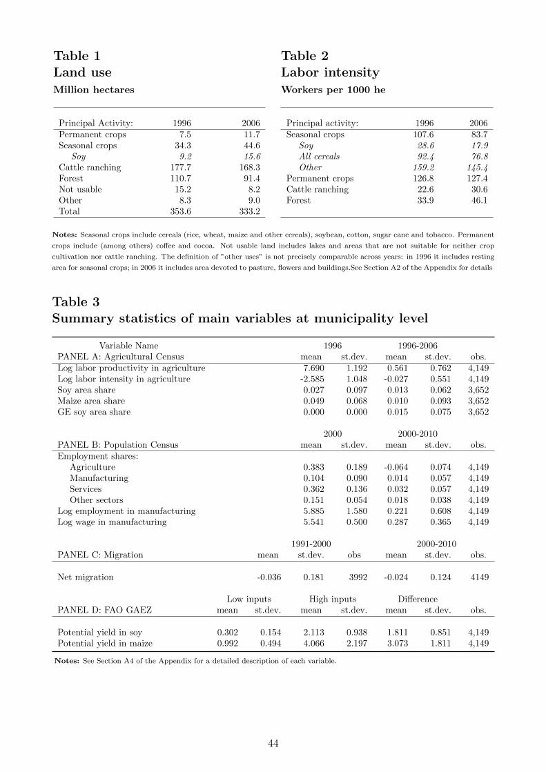
Table 1Land useMillion hectares
Principal Activity: 1996 2006Permanent crops 7.5 11.7Seasonal crops 34.3 44.6
Soy 9.2 15.6Cattle ranching 177.7 168.3Forest 110.7 91.4Not usable 15.2 8.2Other 8.3 9.0Total 353.6 333.2
Table 2Labor intensityWorkers per 1000 he
Principal activity: 1996 2006Seasonal crops 107.6 83.7
Soy 28.6 17.9All cereals 92.4 76.8Other 159.2 145.4
Permanent crops 126.8 127.4Cattle ranching 22.6 30.6Forest 33.9 46.1
Notes: Seasonal crops include cereals (rice, wheat, maize and other cereals), soybean, cotton, sugar cane and tobacco. Permanent
crops include (among others) coffee and cocoa. Not usable land includes lakes and areas that are not suitable for neither crop
cultivation nor cattle ranching. The definition of ”other uses” is not precisely comparable across years: in 1996 it includes resting
area for seasonal crops; in 2006 it includes area devoted to pasture, flowers and buildings.See Section A2 of the Appendix for details
Table 3Summary statistics of main variables at municipality level
Variable Name 1996 1996-2006PANEL A: Agricultural Census mean st.dev. mean st.dev. obs.Log labor productivity in agriculture 7.690 1.192 0.561 0.762 4,149Log labor intensity in agriculture -2.585 1.048 -0.027 0.551 4,149Soy area share 0.027 0.097 0.013 0.062 3,652Maize area share 0.049 0.068 0.010 0.093 3,652GE soy area share 0.000 0.000 0.015 0.075 3,652
2000 2000-2010PANEL B: Population Census mean st.dev. mean st.dev. obs.Employment shares:
Agriculture 0.383 0.189 -0.064 0.074 4,149Manufacturing 0.104 0.090 0.014 0.057 4,149Services 0.362 0.136 0.032 0.057 4,149Other sectors 0.151 0.054 0.018 0.038 4,149
Log employment in manufacturing 5.885 1.580 0.221 0.608 4,149Log wage in manufacturing 5.541 0.500 0.287 0.365 4,149
1991-2000 2000-2010PANEL C: Migration mean st.dev. obs mean st.dev. obs.
Net migration -0.036 0.181 3992 -0.024 0.124 4149
Low inputs High inputs DifferencePANEL D: FAO GAEZ mean st.dev. mean st.dev. mean st.dev. obs.
Potential yield in soy 0.302 0.154 2.113 0.938 1.811 0.851 4,149Potential yield in maize 0.992 0.494 4.066 2.197 3.073 1.811 4,149
Notes: See Section A4 of the Appendix for a detailed description of each variable.
44
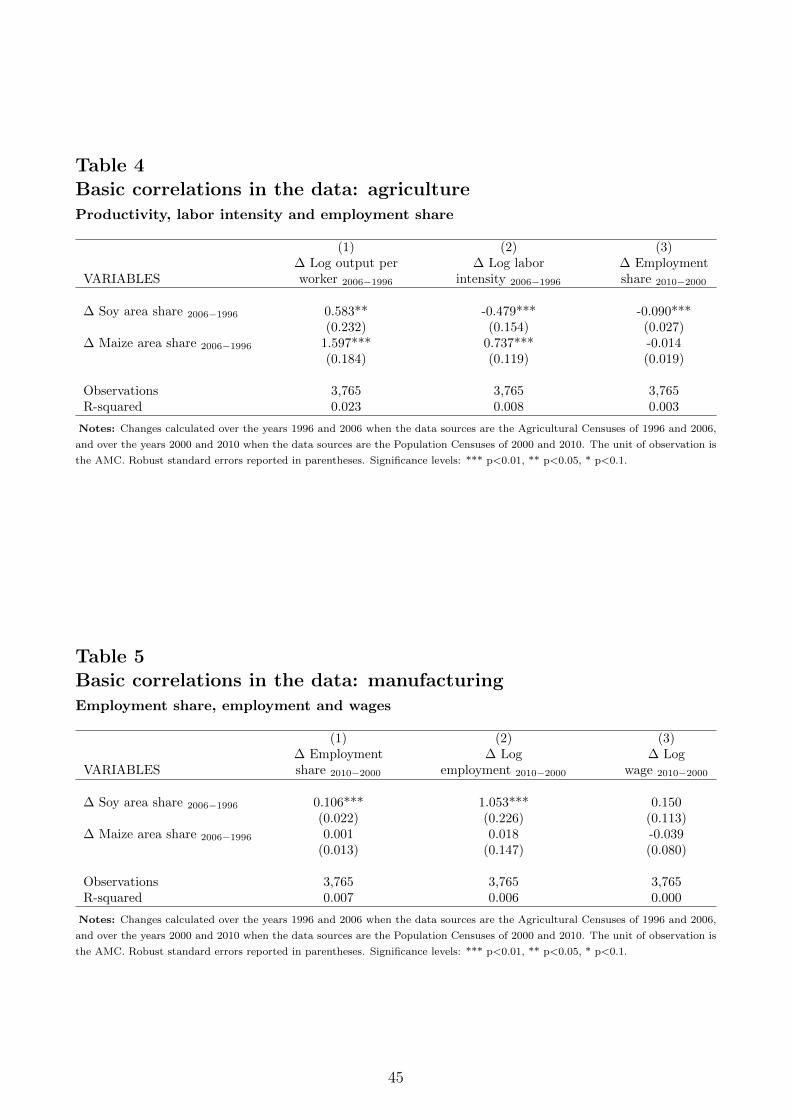
Table 4Basic correlations in the data: agricultureProductivity, labor intensity and employment share
(1) (2) (3)∆ Log output per ∆ Log labor ∆ Employment
VARIABLES worker 2006−1996 intensity 2006−1996 share 2010−2000
∆ Soy area share 2006−1996 0.583** -0.479*** -0.090***(0.232) (0.154) (0.027)
∆ Maize area share 2006−1996 1.597*** 0.737*** -0.014(0.184) (0.119) (0.019)
Observations 3,765 3,765 3,765R-squared 0.023 0.008 0.003
Notes: Changes calculated over the years 1996 and 2006 when the data sources are the Agricultural Censuses of 1996 and 2006,
and over the years 2000 and 2010 when the data sources are the Population Censuses of 2000 and 2010. The unit of observation is
the AMC. Robust standard errors reported in parentheses. Significance levels: *** p<0.01, ** p<0.05, * p<0.1.
Table 5Basic correlations in the data: manufacturingEmployment share, employment and wages
(1) (2) (3)∆ Employment ∆ Log ∆ Log
VARIABLES share 2010−2000 employment 2010−2000 wage 2010−2000
∆ Soy area share 2006−1996 0.106*** 1.053*** 0.150(0.022) (0.226) (0.113)
∆ Maize area share 2006−1996 0.001 0.018 -0.039(0.013) (0.147) (0.080)
Observations 3,765 3,765 3,765R-squared 0.007 0.006 0.000
Notes: Changes calculated over the years 1996 and 2006 when the data sources are the Agricultural Censuses of 1996 and 2006,
and over the years 2000 and 2010 when the data sources are the Population Censuses of 2000 and 2010. The unit of observation is
the AMC. Robust standard errors reported in parentheses. Significance levels: *** p<0.01, ** p<0.05, * p<0.1.
45

Table 6Comparing Municipalities below/above median increase in potentialsoy yield
(1) (2) (3)Below Above Difference
∆Asoy median ∆Asoy median
Agricultural Employment Share 1991 0.500 0.443 -0.057***[0.007]
Manufacturing Employment Share 1991 0.080 0.097 0.017***[0.003]
Share Rural Pop 1991 0.516 0.404 -0.112***[0.007]
Log Income per Capita 1991 4.389 4.656 0.267***[0.018]
Log Pop Density 1991 3.155 3.219 0.064[0.041]
Literacy rate 1991 0.688 0.745 0.057***[0.005]
Observations 2075 2074
Note: Average values of observable characteristics of municipalities that rank below and above the median of ∆Asoy . All
observable characteristics are from the Population Census 1991. Column (3) reports the difference between columns (2) and (1),
along with the standard error and significance level of the difference. Significance levels: *** p<0.01, ** p<0.05, * p<0.1.
46
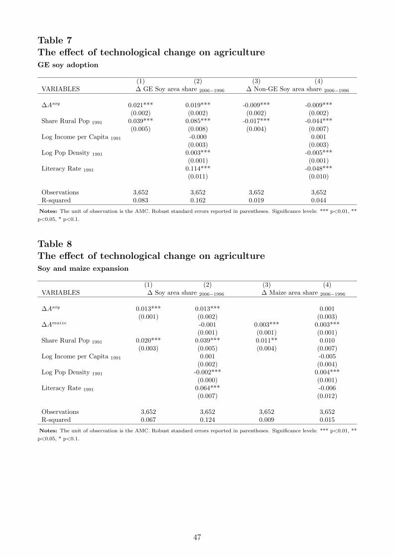
Table 7The effect of technological change on agricultureGE soy adoption
(1) (2) (3) (4)VARIABLES ∆ GE Soy area share 2006−1996 ∆ Non-GE Soy area share 2006−1996
∆Asoy 0.021*** 0.019*** -0.009*** -0.009***(0.002) (0.002) (0.002) (0.002)
Share Rural Pop 1991 0.039*** 0.085*** -0.017*** -0.044***(0.005) (0.008) (0.004) (0.007)
Log Income per Capita 1991 -0.000 0.001(0.003) (0.003)
Log Pop Density 1991 0.003*** -0.005***(0.001) (0.001)
Literacy Rate 1991 0.114*** -0.048***(0.011) (0.010)
Observations 3,652 3,652 3,652 3,652R-squared 0.083 0.162 0.019 0.044
Notes: The unit of observation is the AMC. Robust standard errors reported in parentheses. Significance levels: *** p<0.01, **
p<0.05, * p<0.1.
Table 8The effect of technological change on agricultureSoy and maize expansion
(1) (2) (3) (4)VARIABLES ∆ Soy area share 2006−1996 ∆ Maize area share 2006−1996
∆Asoy 0.013*** 0.013*** 0.001(0.001) (0.002) (0.003)
∆Amaize -0.001 0.003*** 0.003***(0.001) (0.001) (0.001)
Share Rural Pop 1991 0.020*** 0.039*** 0.011** 0.010(0.003) (0.005) (0.004) (0.007)
Log Income per Capita 1991 0.001 -0.005(0.002) (0.004)
Log Pop Density 1991 -0.002*** 0.004***(0.000) (0.001)
Literacy Rate 1991 0.064*** -0.006(0.007) (0.012)
Observations 3,652 3,652 3,652 3,652R-squared 0.067 0.124 0.009 0.015
Notes: The unit of observation is the AMC. Robust standard errors reported in parentheses. Significance levels: *** p<0.01, **
p<0.05, * p<0.1.
47

Table 9The effect of technological change on agricultureProductivity, labor intensity and employment share
(1) (2) (3) (4) (5) (6)∆ Log output per ∆ Log labor ∆ Employment
VARIABLES per worker 2006−1996 intensity 2006−1996 share 2010−2000
∆Asoy 0.115*** 0.131*** -0.057*** -0.064*** -0.018*** -0.021***(0.024) (0.026) (0.018) (0.021) (0.002) (0.002)
∆Amaize -0.025** -0.033*** 0.031*** 0.033*** 0.005*** 0.006***(0.011) (0.011) (0.008) (0.009) (0.001) (0.001)
Share Rural Pop 1991 0.258*** 0.125* -0.136*** -0.177*** -0.091*** -0.076***(0.057) (0.070) (0.048) (0.051) (0.005) (0.007)
Log Income per Capita 1991 -0.010 0.029 0.014***(0.045) (0.039) (0.004)
Log Pop Density 1991 -0.016 -0.017 -0.000(0.011) (0.011) (0.001)
Literacy Rate 1991 -0.270* -0.124 -0.012(0.139) (0.116) (0.014)
Observations 4,149 4,149 4,149 4,149 4,149 4,149R-squared 0.009 0.012 0.005 0.007 0.068 0.073
Notes: Changes calculated over the years 1996 and 2006 when the data sources are the Agricultural Censuses of 1996 and 2006,
and over the years 2000 and 2010 when the data sources are the Population Censuses of 2000 and 2010. The unit of observation is
the AMC. Robust standard errors reported in parentheses. Significance levels: *** p<0.01, ** p<0.05, * p<0.1.
Table 10The effect of agricultural technological change on manufacturingEmployment share, employment and wages
(1) (2) (3) (4) (5) (6)∆ Employment ∆ Log ∆ Log
VARIABLES share 2010−2000 employment 2010−2000 wage 2010−2000
∆Asoy 0.023*** 0.021*** 0.218*** 0.186*** -0.032*** -0.024*(0.002) (0.002) (0.018) (0.020) (0.012) (0.012)
∆Amaize -0.005*** -0.004*** -0.057*** -0.043*** 0.018*** 0.014**(0.001) (0.001) (0.009) (0.009) (0.005) (0.005)
Share Rural Pop 1991 -0.006 0.011** -0.186*** 0.051 0.197*** -0.014(0.004) (0.005) (0.044) (0.056) (0.026) (0.035)
Log Income per Capita 1991 0.002 0.093** -0.107***(0.003) (0.037) (0.026)
Log Pop Density 1991 0.002** 0.020** -0.035***(0.001) (0.008) (0.005)
Literacy Rate 1991 0.034*** 0.197* 0.093(0.010) (0.117) (0.075)
Observations 4,149 4,149 4,149 4,149 4,149 4,149R-squared 0.063 0.073 0.056 0.068 0.022 0.045
Notes: The unit of observation is the AMC. Robust standard errors reported in parentheses. Significance levels: *** p<0.01, **
p<0.05, * p<0.1.
48
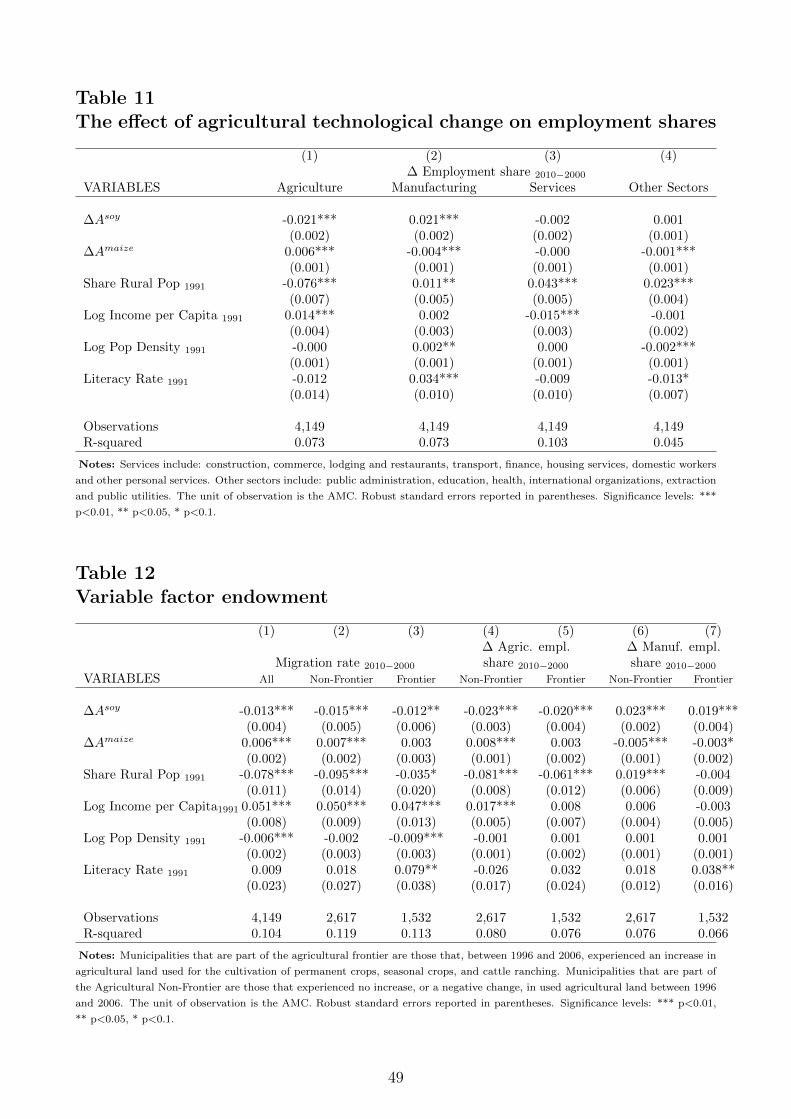
Table 11The effect of agricultural technological change on employment shares
(1) (2) (3) (4)∆ Employment share 2010−2000
VARIABLES Agriculture Manufacturing Services Other Sectors
∆Asoy -0.021*** 0.021*** -0.002 0.001(0.002) (0.002) (0.002) (0.001)
∆Amaize 0.006*** -0.004*** -0.000 -0.001***(0.001) (0.001) (0.001) (0.001)
Share Rural Pop 1991 -0.076*** 0.011** 0.043*** 0.023***(0.007) (0.005) (0.005) (0.004)
Log Income per Capita 1991 0.014*** 0.002 -0.015*** -0.001(0.004) (0.003) (0.003) (0.002)
Log Pop Density 1991 -0.000 0.002** 0.000 -0.002***(0.001) (0.001) (0.001) (0.001)
Literacy Rate 1991 -0.012 0.034*** -0.009 -0.013*(0.014) (0.010) (0.010) (0.007)
Observations 4,149 4,149 4,149 4,149R-squared 0.073 0.073 0.103 0.045
Notes: Services include: construction, commerce, lodging and restaurants, transport, finance, housing services, domestic workers
and other personal services. Other sectors include: public administration, education, health, international organizations, extraction
and public utilities. The unit of observation is the AMC. Robust standard errors reported in parentheses. Significance levels: ***
p<0.01, ** p<0.05, * p<0.1.
Table 12Variable factor endowment
(1) (2) (3) (4) (5) (6) (7)∆ Agric. empl. ∆ Manuf. empl.
Migration rate 2010−2000 share 2010−2000 share 2010−2000
VARIABLES All Non-Frontier Frontier Non-Frontier Frontier Non-Frontier Frontier
∆Asoy -0.013*** -0.015*** -0.012** -0.023*** -0.020*** 0.023*** 0.019***(0.004) (0.005) (0.006) (0.003) (0.004) (0.002) (0.004)
∆Amaize 0.006*** 0.007*** 0.003 0.008*** 0.003 -0.005*** -0.003*(0.002) (0.002) (0.003) (0.001) (0.002) (0.001) (0.002)
Share Rural Pop 1991 -0.078*** -0.095*** -0.035* -0.081*** -0.061*** 0.019*** -0.004(0.011) (0.014) (0.020) (0.008) (0.012) (0.006) (0.009)
Log Income per Capita1991 0.051*** 0.050*** 0.047*** 0.017*** 0.008 0.006 -0.003(0.008) (0.009) (0.013) (0.005) (0.007) (0.004) (0.005)
Log Pop Density 1991 -0.006*** -0.002 -0.009*** -0.001 0.001 0.001 0.001(0.002) (0.003) (0.003) (0.001) (0.002) (0.001) (0.001)
Literacy Rate 1991 0.009 0.018 0.079** -0.026 0.032 0.018 0.038**(0.023) (0.027) (0.038) (0.017) (0.024) (0.012) (0.016)
Observations 4,149 2,617 1,532 2,617 1,532 2,617 1,532R-squared 0.104 0.119 0.113 0.080 0.076 0.076 0.066
Notes: Municipalities that are part of the agricultural frontier are those that, between 1996 and 2006, experienced an increase in
agricultural land used for the cultivation of permanent crops, seasonal crops, and cattle ranching. Municipalities that are part of
the Agricultural Non-Frontier are those that experienced no increase, or a negative change, in used agricultural land between 1996
and 2006. The unit of observation is the AMC. Robust standard errors reported in parentheses. Significance levels: *** p<0.01,
** p<0.05, * p<0.1.
49

Table 13The effect of agricultural technological change on manufacturingEmployment share, employment and wages
Robustness to using a larger unit of observation: micro-regions
(1) (2) (3)∆ Employment ∆ Log ∆ Log
VARIABLES share 2010−2000 employment 2010−2000 wage 2010−2000
∆Asoy 0.017*** 0.139*** -0.022(0.004) (0.029) (0.016)
∆Amaize -0.003 -0.037*** 0.016**(0.002) (0.013) (0.007)
Share Rural Pop 1991 0.014 0.017 -0.103(0.012) (0.121) (0.089)
Log Income per Capita 1991 -0.002 0.058 -0.168**(0.007) (0.088) (0.073)
Log Pop Density 1991 0.004*** 0.030*** -0.032***(0.001) (0.011) (0.007)
Literacy Rate 1991 0.016 0.007 0.128(0.021) (0.261) (0.180)
Observations 557 557 557R-squared 0.101 0.107 0.239
Notes: The unit of observation is the micro-region. Robust standard errors reported in parentheses. Significance levels: ***
p<0.01, ** p<0.05, * p<0.1.
Table 14The effect of agricultural technological change on manufacturingEmployment share, employment and wages
Robustness to excluding sectors directly linked to soy and maize
(1) (2) (3)∆ Employment ∆ Log ∆ Log
VARIABLES share 2010−2000 employment 2010−2000 wage 2010−2000
∆Asoy 0.013*** 0.167*** -0.011(0.002) (0.021) (0.016)
∆Amaize -0.004*** -0.057*** 0.010(0.001) (0.009) (0.007)
Share Rural Pop 1991 0.012*** 0.042 -0.014(0.004) (0.058) (0.044)
Log Income per Capita 1991 -0.002 0.075* -0.117***(0.002) (0.038) (0.027)
Log Pop Density 1991 0.003*** 0.034*** -0.040***(0.000) (0.008) (0.006)
Literacy Rate 1991 0.025*** 0.086 0.144*(0.007) (0.124) (0.084)
Observations 4,149 4,134 4,059R-squared 0.037 0.042 0.030
Notes: Manufacturing sectors directly linked to soy and maize are: food and beverages (code 15), manufacturing of other chemicals
(code 24090) and manufacturing of goods from refined oil (code 23020). The unit of observation is the AMC. Robust standard
errors reported in parentheses. Significance levels: *** p<0.01, ** p<0.05, * p<0.1. The number of observations in columns 2 and
3 is smaller because in some municipalities sectors directly linked to soy and maize account for the whole manufacturing sector.
50

Technical Appendix to Agricultural Productivity and Structural
Transformation: Not for Publication
Paula Bustos, Bruno Caprettini and Jacopo Ponticelli
A1 Introduction
This technical appendix contains a more detailed exposition of the theoretical framework pre-
sented in the paper, a detailed description of the variables used in the empirical analysis as well as
additional supplementary material for the paper. The appendix follows the same structure of the
paper. Section A2 provides additional material on section 2 in the paper. In particular, it provides
a detailed description of the data sources used in the Figures presented in section 2. Section A3
contains the proofs of the propositions stated in section 3 of the paper, and an extension of the
model presented in the paper that includes a non-tradable sector. Section A4 provides a detailed
description of all the variables used in the empirical analysis. In section A5 we report additional
empirical results discussed in section 5 of the paper. Finally, in section A6 we report the tables of
a set of robustness checks described in the paper.
A2 Agriculture in Brazil
In this section we provide additional information on the data used to produce Figure 1 and
Tables 1 and 2 in the paper, which show stylized facts about agriculture in Brazil.
Figure 1: The data used on soy output, area planted with soy and area planted with maize
in first and second season is from CONAB, while data on number of workers employed in soy
production is from PNAD. CONAB, Companhia Nacional de Abastecimento, is an agency within
the Brazilian Ministry of Agriculture. CONAB carries out monthly surveys to monitor the evolution
of the harvest of all major crops in Brazil: the surveys are representative at state level and are
constructed by interviewing on the ground farmers, agronomists and financial agents in the main
cities of the country. All data can be downloaded at: http://www.conab.gov.br/conteudos.php?
a=1252&t=. PNAD is a national household survey representative at state level carried out yearly
by the IBGE (the survey was not carried out in 1994 and in the census years: 1991, 2000 and 2010).
Since the PNAD coverage changed over time, to harmonize the sample across years we exclude from
the PNAD data: (i) workers located in the states of: Rondonia, Acre, Amazonas, Roraima, Para
and Amapa (North macro-region) because only urban areas (and not rural areas) of these states
were covered until 2004; (ii) workers located in the states of: Tocantins, Mato Grosso do Sul, Goias
and the Distrito Federal because the sample of households in these states is not complete in the
years from 1992 to 1997. We harmonized data from CONAB with the PNAD coverage such that
numerator and denominator are constructed using the same subset of states.
Tables 1 and 2: The data on land use and labor intensity in agriculture is from the Brazilian
Agricultural Censuses of 1996 and 2006. The data has been downloaded from the IBGE Sidra
repository. In particular: data on land use is from Table 317 for 1996 and Table 1011 for 2006;
1

data on land in farm by principal activity in 1996 is from Table 491 and for 2006 from table 797;
data on total number of workers in 1996 is reported in Table 321 and in 2006 in Table 956. Notice
that the definition of “principal activity” of the farm changed between the Agricultural Census
of 1996 and the one of 2006. In 1996 higher specialization was required for farms to be classified
under one of the categories reported, and those that did not produce at least 2/3 of the value
within a single category were classified under the “mixed activity” category. In 2006 farms were
classified according to the activity that accounted for the simple majority of production and no
“mixed activity” category existed.
Figure A1 shows the evolution between 1992 and 2009 of the total number of workers (expressed
in million) employed in different sectors of the Brazilian economy.
Figure A1 Employment in agriculture, industry, services (1992-2009)
1020
3040
50
wor
kers
(in
mill
ions
)
1990 1995 2000 2005 2010
year
agriculture manufacturing
services
Notes: Services include: commerce, lodging and restaurants, transport, finance, housing services, other personal
services, domestic workers and construction. Data from PNAD.
2

A3 Model
In this section, we provide derivations of all expressions and results reported in the paper.
A.3.1 Setup
In this section we show that labor-augmenting technical change reduces the marginal product of
labor when the elasticity of substitution is smaller than the land share of output.
We start by obtaining MPLa = ∂Qa∂La
by differentiating the agricultural production function
described by equation (1) w.r.t. labor:
MPLa = ANΘσσ−1−1γL
σ−1σ−1
a Aσ−1σ
L (A.1)
where, to save space, we define Θ ≡ γ (ALLa)σ−1σ + (1 − γ) (ATT )
σ−1σ . Next, we obtain ∂MPLa
∂ALas
follows:∂MPLa∂AL
= ANΘ1
σ−1γL−1σa A
−1σL
σ − 1
σ
[1 +
1
σ − 1Θ−1γ (ALLa)
σ−1σ
].
Then, when σ < 1, σ−1σ < 0. As a result, ∂MPLa
∂AL< 0 iff the last term in brackets is positive, which
is true as long as σ satisfies the following condition:
σ <(1 − γ) (ATT )
σ−1σ
γ (ALLa)σ−1σ + (1 − γ) (ATT )
σ−1σ
=TaMPTa
Qa≡ 1 − Γ. (A.2)
Note that this condition is a function of the equilibrium level of employment in agriculture. In
particular, in the relevant case where σ < 1 the land share (1 − Γ) is increasing on the level
of agricultural employment. As a result, the condition is more likely to be satisfied when the
equilibrium level of agricultural employment is high.
A.3.2 Equilibrium
In this section we detail the derivations necessary to obtain the equilibrium level of employment in
agriculture. First, note that profit maximization implies that the value of the marginal product of
labor must equal the wage in both sectors: PaMPLa = w = PmMPLm. Thus, the marginal product
of labor in agriculture is determined by international prices and manufacturing productivity:
MPLa =
(PmPa
)∗Am. (A.3)
Next, starting from equation A.1, and using the land market clearing condition (Ta = T ), MPLa
can be written as follows:
MPLa = ANALγ
[γ + (1 − γ)
(ATT
ALLa
)σ−1σ
] 1σ−1
. (A.4)
3

Then, A.3 and A.4 can be used to solve for the equilibrium level of employment in agriculture:
L∗a =ATT
AL
{γ
1 − γ
[1
γσ
(PaPm
ANALAm
)1−σ− 1
]} σ1−σ
. (1)
Next, we obtain equation (4), where L∗a is written as a function of the equilibrium land share. We
calculate the ratio of the labor to land share using the production function described by equation
(1):
Γ
1 − Γ≡
LaMPLaQa
TaMPTaQa
=γ
(1 − γ)
(ALLaATT
)σ−1σ
. (A.6)
Note that the equalization of the value of the marginal product of labor across sectors, described
by equations A.3 and A.4, implies:
(1 − γ)
γ
(ATT
ALLa
)σ−1σ
=1
γ
(PmPa
AmANγAL
)σ−1
− 1. (A.7)
Equations A.6 and A.7 can be used to obtain a solution for the the equilibrium land share. This
solution implies that the parameter restriction necessary for labor augmenting technical change to
be strongly labor saving is:
σ < 1 − Γ∗ = 1 − γ
(PmPa
AmANγAL
)1−σ. (A.8)
Note that as σ gets closer to one, 1 − Γ∗ converges to the parameter 1 − γ. In the relevant case
where σ < 1, the land share is increasing in world relative prices for agricultural goods and relative
agricultural productivity. Thus, this condition is more likely to be satisfied in regions with a
comparative advantage in agriculture.
A.3.3 Technological Change and Structural Transformation
In this section we analyze the response of agricultural and manufacturing employment to labor-
augmenting technical change.
Labor-augmenting technical change
The effect of labor augmenting technical change on agricultural employment depends on whether
the elasticity of substitution is smaller than the equilibrium land share of agricultural production
(σ < 1−Γ∗). When this condition is satisfied, we say that land and labor are strong complements.
a) Land and labor are strong complements: ∂L∗a
∂AL< 0 and ∂L∗
m∂AL
> 0.
Proof. We obtain ∂L∗a
∂ALfrom the solution for L∗a as a function of the equilibrium land share given
4

by equation (6), as follows:
∂L∗a∂AL
=
(γ
1 − γ
) σ1−σ
(1 − Γ∗
Γ∗
) σ1−σ ATT
A2L
{σ
1 − σ
∂ 1−Γ∗
Γ∗
∂AL
AL1−Γ∗
Γ∗− 1
}(A.9)
=
(γ
1 − γ
) σ1−σ
(1 − Γ∗
Γ∗
) σ1−σ ATT
A2L
{σ
1 − Γ∗− 1
}
where the last step used the following solution for the elasticity of the land to labor share ratio
with respect to labor-augmenting technical change:
∂ 1−Γ∗
Γ∗
∂AL
AL1−Γ∗
Γ∗=
1 − σ
1 − Γ∗. (A.10)
Equation A.9 implies that ∂L∗a
∂AL< 0 iff σ
1−Γ∗ < 1. In this case, ∂L∗m
∂AL> 0 because L∗a + L∗m = L.
b) Land and labor are not strong complements: ∂L∗a
∂AL> 0 and ∂L∗
m∂AL
< 0.
Proof. A.9. implies ∂L∗a
∂AL> 0 iff σ
1−Γ∗ > 1. In this case, ∂L∗m
∂AL< 0 because L∗a + L∗m = L.
A.3.4 Empirical Predictions
Prediction 1. If land and labor are strong complements in production, labor augmenting technical
change in agriculture (AL) :
(a) increases the value of output per worker:∂P∗aQ
∗a
L∗a
∂AL> 0;
(b) reduces the labor intensity of production:∂L∗aT
∂AL< 0;
(c) reduces the employment share of agriculture:∂L∗aL
∂AL< 0;
(d) increases the employment share of manufacturing:∂L∗mL
∂AL> 0.
Proof
(a) We start by obtaining the average product of labor QaLa
by dividing the agricultural produc-
tion function described by equation (2) by La :
QaLa
= AaAL
[γ + (1 − γ)
(ATTaALLa
)σ−1σ
] σσ−1
.
Next, we use equation (A.4) to write QaLa
as a function of the marginal product of labor, as follows:
QaLa
= γ−σ (ANAL)1−σ (MPLa)σ . (A.11)
The equation above implies that an increase in AL must increase the equilibrium average product
of labor as long as σ < 1. This is because the marginal product of labor must remain constant in
5

equilibrium (see condition A.3 above). Finally, because prices are set in international markets, the
value of the average product of labor also increases.
(b) and (c) Note that ∂L∗a
∂AL< 0, as shown in section 3.3. As a result,
∂L∗aT
∂AL< 0 because the land
endowment is fixed;∂L∗aL
∂AL< 0 and because the labor endowment is fixed.
(d) Note that ∂L∗m
∂AL> 0, as shown in section 3.3. As a result,
∂L∗mL
∂AL< 0 because the labor
endowment is fixed.
Prediction 2. Land augmenting technical change in agriculture (AT ) :
(a) does not change the value of output per worker:∂P∗aQ
∗a
L∗a
∂AT= 0;
(b) increases the labor intensity of production:∂L∗aT
∂AT> 0;
(c) increases the employment share of agriculture:∂L∗aL
∂AT> 0;
(d) reduces the employment share of manufacturing:∂L∗mL
∂AT< 0.
Proof
(a) This result is implied by equations A.3 and A.11: labor augmenting technical change must
leave the equilibrium marginal product of labor unchanged, as a result, the average product of
labor is also unchanged. Finally, because prices are set in international markets, the value of the
average product of labor is also unchanged.
(b), (c) and (d) These results can be shown with arguments similar to the ones used to prove
prediction 1 above.
A.3.5 Services
In this section we provide an analysis of the model with services.
Setup
The economy is identical to the one described in section 3.1, except that there are three sectors
(goods): agriculture (a), manufacturing (m) and services (s). Agriculture and manufacturing are
tradable, while services are not.
Production
The production function in services uses only labor and displays constant returns to scale:
Qs = AsLs
Production functions in agriculture and manufacturing are described by equations 1 and 2, respec-
tively.
Consumption
Because services are non-tradable, production can no longer be determined independently of con-
sumption. Thus, we specify preferences and factor ownership. Consumers have the following
6

Cobb-Douglas preferences over the three goods:
U(ca, cm, cs) = cαaa cαmm cαss . (A.12)
where αa +αm +αs = 1.1 There are-two types of agents in the economy: L workers, each endowed
with one unit of labor; and T land-owners, each endowed with one unit of land. We assume that
workers reside in the same region where they work. In contrast, land owners can reside in any
region. We denote by θ the share of land owners residing in the same region where their land is
located. Then, aggregate service consumption in a region is Cs = cs,L L+ cs,T θT, where cs,L the
is consumption of workers and cs,T the consumption of land-owners.2,3
Equilibrium
The following equilibrium conditions determine the sectorial allocation of employment:
1. Profit maximization implies that if there is positive employment in all sectors in equilibrium,
the value of the marginal product of labor is equalized across the three sectors:
PaMPLa = w = PmMPLm = PsMPLs. (A.13)
As a result, the wage is determined by value of the marginal product of labor in manufacturing:
w∗ = PmAm.
Finally, the value of the marginal product of land in agriculture is equal to the land rental rate:
r = PaMPTa.
2. Consumer maximization: workers and land owners maximize utility described by A.12 subject
to the constraint paca + pmcm + pscs = yi where yL = w and yT = r.
3. Services market clearing: Qs = Cs
4. Labor market clearing: Lm + La + Ls = L
Employment in agriculture
Note that in an equilibrium with positive manufacturing employment the condition PaMPLa =
w∗ = PmAm still defines equilibrium employment in agriculture. Thus, L∗a is still given by equation
1Our use of an homotetic utility function follows the findings in Herrendorf, Rogerson and Valentinyi (2013). Theyshow that an homotetic utility function where the elasticity of substitution across sectors is smaller than one providesthe best fit to the Postwar U.S. data when sectoral consumption data is measured in terms of value added. Becausewe use data on employment to measure structural transformation, our analysis tracks value added better than finalgoods consumption. As a result we use a non-homotetic utility function. However, we assume that the elasticity ofsubstitution across sectors is equal to one to make the model simpler. We discuss below how the predictions of ourmodel would be modified if this elasticity was smaller than one.
2Note that θ is the share of services consumption of land owners that is spent locally. Thus, an alternativeinterpretation is that land-owners reside locally but consume some services in other regions.
3Note that we are not taking into account the local consumption of land owners who reside in the region underconsideration but own land in other regions. The reason for this ommision is that, in the model, their demand forservices would not be affected by technical change in the region where they live but in the region where they ownland.
7
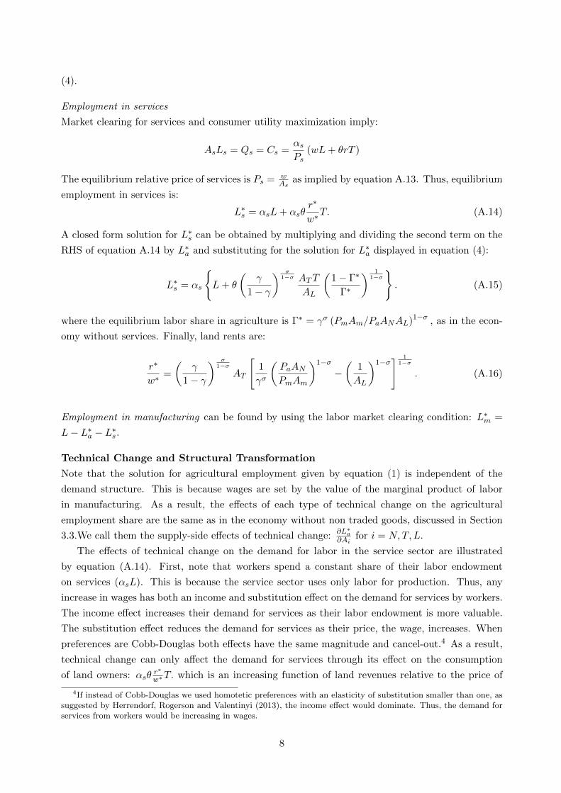
(4).
Employment in services
Market clearing for services and consumer utility maximization imply:
AsLs = Qs = Cs =αsPs
(wL+ θrT )
The equilibrium relative price of services is Ps = wAs
as implied by equation A.13. Thus, equilibrium
employment in services is:
L∗s = αsL+ αsθr∗
w∗T. (A.14)
A closed form solution for L∗s can be obtained by multiplying and dividing the second term on the
RHS of equation A.14 by L∗a and substituting for the solution for L∗a displayed in equation (4):
L∗s = αs
{L+ θ
(γ
1 − γ
) σ1−σ ATT
AL
(1 − Γ∗
Γ∗
) 11−σ}. (A.15)
where the equilibrium labor share in agriculture is Γ∗ = γσ (PmAm/PaANAL)1−σ , as in the econ-
omy without services. Finally, land rents are:
r∗
w∗=
(γ
1 − γ
) σ1−σ
AT
[1
γσ
(PaANPmAm
)1−σ−(
1
AL
)1−σ] 1
1−σ
. (A.16)
Employment in manufacturing can be found by using the labor market clearing condition: L∗m =
L− L∗a − L∗s.
Technical Change and Structural Transformation
Note that the solution for agricultural employment given by equation (1) is independent of the
demand structure. This is because wages are set by the value of the marginal product of labor
in manufacturing. As a result, the effects of each type of technical change on the agricultural
employment share are the same as in the economy without non traded goods, discussed in Section
3.3.We call them the supply-side effects of technical change: ∂L∗a
∂Aifor i = N,T, L.
The effects of technical change on the demand for labor in the service sector are illustrated
by equation (A.14). First, note that workers spend a constant share of their labor endowment
on services (αsL). This is because the service sector uses only labor for production. Thus, any
increase in wages has both an income and substitution effect on the demand for services by workers.
The income effect increases their demand for services as their labor endowment is more valuable.
The substitution effect reduces the demand for services as their price, the wage, increases. When
preferences are Cobb-Douglas both effects have the same magnitude and cancel-out.4 As a result,
technical change can only affect the demand for services through its effect on the consumption
of land owners: αsθr∗
w∗T. which is an increasing function of land revenues relative to the price of
4If instead of Cobb-Douglas we used homotetic preferences with an elasticity of substitution smaller than one, assuggested by Herrendorf, Rogerson and Valentinyi (2013), the income effect would dominate. Thus, the demand forservices from workers would be increasing in wages.
8

services in trems of labor ( r∗
w∗ ). Thus, the effects of agricultural technical change on employment in
the service sector depend on its effect on land rents. In turn, agricultural technical change always
increases land rents, as we show below. As a result, the demand for services and employment in the
service sector increase. We call this the demand side effects of technical change: ∂L∗s
∂Aifor i = N,T, L.
In what follows, we show that when technical change is Hicks-neutral or land-augmenting,
both the supply-side and demand-side effects reduce manufacturing employment. However, when
technical change is strongly labor-saving each effect moves manufacturing employment in opposite
directions. On the one hand, the supply side effect releases labor from agriculture, increasing
the labor supply for manufacturing. On the other hand, the demand-side effect increases labor
demand in services, reducing the supply of labor for manufacturing. As a result, the net effect on
manufacturing employment depends on the relative strength of each effect. In the appendix, we
show that the supply-side effect dominates as long as σ < (1 − Γ∗) (1 − αsθ) . Note that because
1−αsθ < 1, this condition is stronger than the condition required for agricultural technical change
to be strongly labor-saving : σ < 1−Γ∗. Thus, it is satisfied as long as land-owners’s consumption
share of local services (αsθ) is not too large.
Labor-augmenting technical change
a) Land and labor are strong complements:
a.1) ∂L∗a
∂AL< 0, ∂L∗
s∂AL
> 0, and ∂L∗m
∂AL> 0 if σ < (1 − Γ∗) (1 − αsθ)
a.2) ∂L∗a
∂AL< 0, ∂L∗
s∂AL
> 0, and ∂L∗m
∂AL< 0 if (1 − Γ∗) (1 − αsθ) < σ < (1 − Γ∗) .
Proof: As shown in section 3.3, when σ < 1 − Γ∗ labor augmenting technical change generates a
reallocation of labor away from agriculture. Then, the labor market clearing condition implies that
Lm + Ls must increase. In addition, ∂L∗s
∂AL≥ 0 because land rents increase: ∂ r∗
w∗�∂AL > 0, see
equations (A.14) and (A.16). Finally, the effects of technical change on manufacturing employment
depend on whether the increase in the demand for labor in the service sector is larger than the
reduction in agricultural employment, given by equation A.9. To make this comparison we obtain∂L∗
s∂AL
from the solution for L∗s given by equation (A.15), as follows:
∂L∗s∂AL
= αsθ
(γ
1 − γ
) σ1−σ
{−ATTA2L
(1 − Γ∗
Γ∗
) 11−σ
+1
1 − σ
ATT
AL
(1 − Γ∗
Γ∗
) 11−σ−1 ∂ 1−Γ∗
Γ∗
∂AL
}
= αsθ
(γ
1 − γ
) σ1−σ
(1 − Γ∗
Γ∗
) σ1−σ ATT
A2L
where the last step used the solution for the elasticity of the land to labor share ratio with respect
to labor-augmenting technical change given by equation (A.10). Then, ∂L∗m
∂AL> 0 as long as − ∂L∗
a∂AL
>∂L∗
s∂AL
, which requires the following parameter restriction:
σ < (1 − Γ∗) (1 − αsθ) . (A.17)
b) Land and labor are not strong complements: ∂L∗a
∂AL> 0, ∂L∗
s∂AL
≥ 0, and ∂L∗m
∂AL< 0.
9

Proof: As shown in section 3.3, when σ ≥ 1 − Γ∗ labor augmenting technical change generates
a reallocation of labor into agriculture. Then, the labor market clearing condition implies that
Lm +Ls must fall. In addition, ∂L∗s
∂AL≥ 0 because land rents increase: ∂ r∗
w∗�∂AL > 0, see equations
(A.14) and (A.16). As a result, manufacturing employment falls.
Land-augmenting technical change: ∂L∗a
∂AT> 0, ∂L∗
s∂AT
≥ 0, and ∂L∗m
∂AT< 0.
Proof: See equations (1), (A.14), (A.16), and the labor market clearing condition.
Hicks-neutral technical change: ∂L∗a
∂AN> 0, ∂L∗
s∂AN
≥ 0, and ∂L∗m
∂AN< 0.
Proof: See equations (1), (A.14), (A.16), and the labor market clearing condition.
10

A4 Data
This section contains a detailed description of the main variables used in the empirical section
of the paper.
Value of output per worker in agriculture. Data on value of agricultural production per
worker is from the Brazilian Agricultural Census (IBGE (1996,2006)) and it is sourced from the
IBGE online data repository SIDRA.5. The variable ”value of output per worker in agriculture”
is defined as the logarithm of total value of agricultural production divided by the total number
of workers employed in agriculture. Total value of production in agriculture in 1996 comes from
tables: 500 (value of production by seasonal crop), 513 (value of production by permanent crop),
527 (value of production by horticulture product), 534 (value of production by forestry product),
551 (value of production by vegetable extraction product) and 338 (value of animals by type).
Total value of production in agriculture in 2006 comes from tables: 1823 (value of production by
seasonal crop), 1177/1178 (value of production by permanent crop), 818 (value of production by
horticulture product), 815 (value of production by forestry product), 816 (value of production by
vegetable extraction product), 782 (value of bovines), 937 (value of swines), 943 (value of poultry).
Number of workers in agriculture comes from table 321 in 1996 and table 956 in 2006. In Tables
A1 and A2 we also use as a control for the initial level of agricultural productivity the value of
output per worker in agriculture from the 1985 Agricultural Census. Data for the 1985 Census was
manually extracted from the original documentation available from the IBGE online library.6 Total
value of production in agriculture in 1985 comes from table 96 (expenditures, value of production
and revenues), while number of workers in agriculture comes from table 87.
The definition of agricultural workers in the Agricultural Censuses of 1996 and 2006 deserves a
more detailed discussion. This variable includes: employees, family members employed in farm ac-
tivities, sharecroppers and people who reside in the farm and perform agricultural activities without
a formal contract. Receiving a wage is not a necessary condition to be considered an agricultural
worker, so subsistence farmers are also included in this definition. In addition, workers that perform
non-agricultural activities within the farm, such as truck drivers, accountants, mechanics or any
other worker performing tasks in support of the main activity of the farm are counted as agricul-
tural workers. Instead, family members or farm residents who were not employed in farm activities,
domestic workers that are employed within the household of the owner but are not assigned agri-
cultural tasks, and workers that are hired by a service provider company that has a contract with
the farm are not counted as agricultural workers. There are two potential issues with this definition
of agricultural workers in the Agricultural Census. The first issue is about how seasonal workers
are accounted for. In particular, there is a potential double counting problem for seasonal workers
that work in more than one farm. This is because the variable is collected at farm level, and not
at individual level, and the definition of agricultural workers includes both permanent (employed
for at least 180 days during the Census year) and seasonal workers, even when the latter are not
employed on the reference date of the Census (p. 53, IBGE, 2006). Therefore, if seasonal workers
are employed by more than one farm during a year, and they are recorded by each of them in the
5At www.sidra.ibge.gov.br.6At www.biblioteca.ibge.gov.br
11
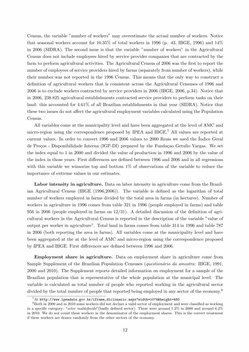
Census, the variable ”number of workers” may overestimate the actual number of workers. Notice
that seasonal workers account for 10.35% of total workers in 1996 (p. 43, IBGE, 1996) and 14%
in 2006 (SIDRA). The second issue is that the variable ”number of workers” in the Agricultural
Census does not include employees hired by service provider companies that are contracted by the
farm to perform agricultural activities. The Agricultural Census of 2006 was the first to report the
number of employees of service providers hired by farms (separately from number of workers), while
their number was not reported in the 1996 Census. This means that the only way to construct a
definition of agricultural workers that is consistent across the Agricultural Censuses of 1996 and
2006 is to exclude workers contracted by service providers in 2006 (IBGE, 2006, p.34). Notice that
in 2006, 238.825 agricultural establishments contracted service providers to perform tasks on their
land: this accounted for 4.61% of all Brazilian establishments in that year (SIDRA). Notice that
these two issues do not affect the agricultural employment variables calculated using the Population
Census.
All variables come at the municipality level and have been aggregated at the level of AMC and
micro-region using the correspondence proposed by IPEA and IBGE.7 All values are reported at
current values. In order to convert 1996 and 2006 values to 2000 Reais we used the Indice Geral
de Precos - Disponibilidade Interna (IGP-DI) prepared by the Fundacao Getulio Vargas. We set
the index equal to 1 in 2000 and divided the value of production in 1996 and 2006 by the value of
the index in those years. First differences are defined between 1996 and 2006 and in all regressions
with this variable we winsorize top and bottom 1% of observations of the variable to reduce the
importance of extreme values in our estimates.
Labor intensity in agriculture. Data on labor intensity in agriculture come from the Brazil-
ian Agricultural Census (IBGE (1996,2006)). The variable is defined as the logarithm of total
number of workers employed in farms divided by the total area in farms (in hectares). Number of
workers in agriculture in 1996 comes from table 321 in 1996 (people employed in farms) and table
956 in 2006 (people employed in farms on 12/31). A detailed discussion of the definition of agri-
cultural workers in the Agricultural Census is reported in the description of the variable ”value of
output per worker in agriculture”. Total land in farms comes from table 314 in 1996 and table 787
in 2006 (both reporting the area in farms). All variables come at the municipality level and have
been aggregated at the at the level of AMC and micro-region using the correspondence proposed
by IPEA and IBGE. First differences are defined between 1996 and 2006.
Employment share in agriculture. Data on employment share in agriculture come from
Sample Supplement of the Brazilian Population Censuses (questionario da amostra: IBGE, 1991,
2000 and 2010). The Supplement reports detailed information on employment for a sample of the
Brazilian population that is representative of the whole population at the municipal level. The
variable is calculated as total number of people who reported working in the agricultural sector
divided by the total number of people that reported being employed in any sector of the economy.8
7At http://www.ipeadata.gov.br/iframe_dicionario.aspx?width=1074&height=4808Both in 2000 and in 2010 some workers did not declare a valid sector of employment and were classified as working
in a specific category: “setor maldefinido”(badly defined sector). These were around 1.2% in 2000 and around 6.2%in 2010. We do not count these workers in the denominator of the employment shares. This is the correct treatmentif these workers are drawn randomly from the other sectors of the economy.
12

Sector of employment is reported according to the first version of the CNAE-Domiciliar in both
2000 and 2010. We define the agricultural sector as any sector with code from 01000 through 09999
(section “A”: agricultura, pecuaria, silvicultura e exploracao florestal and section “B”: pesca).
Notice that this definition includes also workers that are employed by firms that provide services
related to agriculture (code 01401 in the CNAE Domiciliar). In the year 1991 sector of employment
is reported according to the old classification. For these years, we define the agricultural sector as
any sector with code from 010 through 049: these include both agriculture and fishery. In every
year, the sector of activity refers to the sector of the firm where the worker is employed, even if the
worker performs a task that is not directly related to this activity. Employed people are defined as
anyone who reported being employed during the reference week, both in permanent and seasonal
jobs. People who during the reference week worked for no compensation helping someone else in
the household and people who worked in agriculture or fishery for subsistence are also counted
as employed. People who suspended work during the reference week for holidays, strike or leave
are also considered as employed. Original data come at the individual level: we aggregate these
data at the municipality level using the individual weights provided by the IBGE. Data at the
municipality level have been in turn aggregated at the at the level of AMC and micro-region using
the correspondence proposed by IPEA and IBGE. First differences are defined between 2000 and
2010. We do not define first differences between 1991 and 2000 because between these two years
the IBGE changed its definition of employment in two ways. First, it started to count zero-income
workers as employed. Second, the IBGE changed the reference period for considering a person
employed: while in 1991 such period included the last 12 months, in 2000 it only included the
reference week of the Census. Since these changes made the definition of total employment not
homogeneous between 1991 and 2000, we do not compute changes in the employment shares. See
text for further details.
Employment share in manufacturing. Data on employment share in manufacturing come
from Sample Supplement of the Brazilian Population Censuses (questionario da amostra: IBGE,
2000 and 2010). The Supplement reports detailed information on employment for a sample of the
Brazilian population that is representative of the whole population at the municipal level. The
variable is calculated as total number of people who reported working in the manufacturing sector
divided by the total number of people that reported being employed in any sector of the economy.9
Sector of employment is reported according to the first version of the CNAE-Domiciliar in both
2000 and 2010. We define the manufacturing sector as any sector with code from 15000 through
37999 (section “D”: industrias de transformacao). In every year, the sector of activity refers to
the sector of the firm where the worker is employed, even if the worker performs a task that is not
directly related to this sector. Since 2000, employed people are defined as anyone who reported
being employed during the reference week, both in permanent and seasonal jobs. People who during
the reference week worked for no compensation helping someone else in the household and people
who worked in agriculture or fishery for subsistence are also counted as employed people. People
9Both in 2000 and in 2010 some workers did not declare a valid sector of employment and were classified as workingin a specific category: “setor maldefinido”(badly defined sector). These were around 1.2% in 2000 and around 6.2%in 2010. We do not count these workers in the denominator of the employment shares.
13
who suspended work during the reference week for holidays, strike or leave are also considered as
employed. Original data come at the individual level: we aggregate these data at the municipality
level using the individual weights provided by the IBGE. Data at the municipality level have been
in turn aggregated at the at the level of AMC and micro-region using the correspondence proposed
by IPEA and IBGE. First differences are defined between 2000 and 2010.
Employment in manufacturing. Data on employment in manufacturing come from Sample
Supplement of the Brazilian Population Censuses (questionario da amostra: IBGE, 1991, 2000 and
2010). The Supplement reports detailed information on employment for a sample of the Brazilian
population that is representative of the whole population at the municipal level. The variable is
defined as the logarithm of the total number of people who reported working in the manufacturing
sector. Sector of employment is reported according to the first version of the CNAE-Domiciliar
in both 2000 and 2010. For these years, we define the manufacturing sector as any sector with
code from 15000 through 37999 (section “D”: industrias de transformacao). In the years 1991
and 2000 sector of employment is reported according to the old classfication. For these years, we
define the manufacturing sector as any sector with code from 100 through 300. In every year,
the sector of activity refers to the sector of the firm where the worker is employed, even if the
worker performs an activity that is not directly related to this sector. Employed people are defined
as anyone who reported being employed during the reference week. People who suspended work
during the reference week for holidays, strike or leave are also considered as employed. Original data
come at the individual level: we aggregate these data at the municipality level using the individual
weights provided by the IBGE. Data at the municipality level have been in turn aggregated at
the at the level of AMC and micro-region using the correspondence proposed by IPEA and IBGE.
First differences are defined between 2000 and 2010 and between 1991 and 2000 for the pre-trends
regression discussed in section 6.2 and presented in table A3.
Wage in manufacturing. Data on the wage in manufacturing come from Sample Supplement
of the Brazilian Population Censuses (questionario da amostra: IBGE, 1991, 2000 and 2010). The
Supplement reports detailed information on income from employment for a sample of the Brazilian
population that is representative of the whole population at the municipal level. The variable is
calculated as the logarithm of the average wage of manufacturing workers 10 years or older in
2000 Reais. See the discussion of employment in manufacturing for details on the definition of the
manufacturing sector. The Sample Supplement reports the income from the principal job of every
worker. We estimate the average wage in every municipality by looking only to the income from the
principal job of workers who report being employees (empregado com carteira de trabalho assinada
or empregado sem carteira de trabalho assinada): this excludes entrepreneurs and self-employed
workers, whose income from the principal job may include profits or rents but it includes informal
workers.10 Average wage of manufacturing workers at the municipality level is calculated as the
weighted average of the wage of all employees who report working in the manufacturing sector as
principal job, using the individual weights provided by the IBGE. Average wage at the level of AMC
10Income of entrepreneurs and self-employed workers is reported to the Census as business revenues minus businessexpenses.
14

(micro-region) is calculated as a weighted average of the income in all municipalities belonging to
an AMC (micro-region) using the number of manufacturing employees in every municipality as
weight. All wages are reported in current values of the currency in circulation in the year of the
Census: these are thousand Cruzeiros in 1991 and Reais in 2000 and 2010. In order to convert
1991 values to Reais we divided wages in thousand Cruzeiros by 2.75 million. In order to deflate all
current values to July 2000 Reais we used the monthly Indice Nacional de Precos ao Consumidor
(INPC). We set the index equal to 1 in July 2000 (the reference month for the 2000 Census) and
divided the 1991 values in Reais by the INPC index in August 1991 (the reference month for the
1991 Census) and the 2010 values by the INPC index in July 2010 (the reference month for the
2010 Census). First differences are defined between 2000 and 2010 and between 1991 and 2000 for
the pre-trends regression discussed in section 6.2 and presented in table A3.
Share of agricultural land cultivated with soy. Data on the share of agricultural land
cultivated with soy come from the Brazilian Agricultural Census (IBGE (1996,2006)). The variable
is defined as area reaped with soy divided by total land in farms. Area reaped with soy comes from
table 501 in 1996 (area colhida por produtos das lavouras temporarias e condicao do produtor);
and table 1823 in 2006 (producao, venda, valor da producao e area colhida da lavoura temporaria
por produtos da lavoura temporaria e grupos e classes de atividade). Total land in farms comes
from table 314 in 1996 (area dos estabelecimentos por grupo de atividade economica e condicao
legal das terras) and table 787 in 2006 (numero de estabelecimentos e area dos estabelecimentos
agropecuarios, por condicao legal do produtor em relacao as terras, sexo do produtor, grupos de
atividade economica e grupos de area total). All variables come at the municipality level and have
been aggregated at the at the level of AMC and micro-region using the correspondence proposed
by IPEA and IBGE. First differences are defined between 1996 and 2006 and in all regressions
with this variable we windsorize top and bottom 1% of observations of the variable to reduce the
windsorize top and bottom 1% of observations of the variable to reduce the importance of extreme
values in our estimates.
Share of agricultural land cultivated with maize. Data on the share of agricultural
land cultivated with maize come from the Brazilian Agricultural Census (IBGE (1996,2006)). The
variable is defined as area reaped with maize divided by total land in farms. Area reaped with
maize comes from table 501 in 1996 (area colhida por produtos das lavouras temporarias e condicao
do produtor); and table 1823 in 2006 (producao, venda, valor da producao e area colhida da lavoura
temporaria por produtos da lavoura temporaria e grupos e classes de atividade). Total land in farms
comes from table 314 in 1996 (area dos estabelecimentos por grupo de atividade economica e condicao
legal das terras) and table 787 in 2006 (numero de estabelecimentos e area dos estabelecimentos
agropecuarios, por condicao legal do produtor em relacao as terras, sexo do produtor, grupos de
atividade economica e grupos de area total). All variables come at the municipality level and have
been aggregated at the at the level of AMC and micro-region using the correspondence proposed
by IPEA and IBGE. First differences are defined between 1996 and 2006 and in all regressions
with this variable we windsorize top and bottom 1% of observations of the variable to reduce the
importance of extreme values in our estimates.
15
Share of agricultural land cultivated with genetically engineered soy. Data on the
share of agricultural land cultivated with genetically engineered (GE) soy come from the Brazilian
Agricultural Census (IBGE (1996,2006)). The variable is defined as area reaped with GE soy
divided by total land in farms. Area reaped with GE soy comes from table 824 in 2006 (producao,
venda, valor da producao e area colhida da lavoura temporaria por produtos da lavoura temporaria,
tipo de semente, tipo de colheita, tipo de cultivo e destino da producao) and it is assumed to be 0
in 1996. Total land in farms comes from table 314 in 1996 (area dos estabelecimentos por grupo de
atividade economica e condicao legal das terras) and table 787 in 2006 (numero de estabelecimentos
e area dos estabelecimentos agropecuarios, por condicao legal do produtor em relacao as terras,
sexo do produtor, grupos de atividade economica e grupos de area total). All variables come at the
municipality level and have been aggregated at the at the level of AMC and micro-region using the
correspondence proposed by IPEA and IBGE. First differences are defined between 1996 and 2006
and in all regressions with this variable we windsorize top and bottom 1% of observations of the
variable to reduce the importance of extreme values in our estimates.
Share of agricultural land cultivated with traditional soy. Data on the share of agricul-
tural land cultivated with traditional (non-GE) soy come from the Brazilian Agricultural Census
(IBGE (1996,2006)). The variable is defined as area reaped with soy minus the area reaped with GE
soy divided by total land in farms. Area reaped with soy comes from table 501 in 1996 (area colhida
por produtos das lavouras temporarias e condicao do produtor); and table 1823 in 2006 (producao,
venda, valor da producao e area colhida da lavoura temporaria por produtos da lavoura temporaria
e grupos e classes de atividade). Area reaped with GE soy comes from table 824 in 2006 (producao,
venda, valor da producao e area colhida da lavoura temporaria por produtos da lavoura temporaria,
tipo de semente, tipo de colheita, tipo de cultivo e destino da producao) and it is assumed to be 0
in 1996. Total land in farms comes from table 314 in 1996 (area dos estabelecimentos por grupo de
atividade economica e condicao legal das terras) and table 787 in 2006 (numero de estabelecimentos
e area dos estabelecimentos agropecuarios, por condicao legal do produtor em relacao as terras,
sexo do produtor, grupos de atividade economica e grupos de area total). All variables come at the
municipality level and have been aggregated at the at the level of AMC and micro-region using the
correspondence proposed by IPEA and IBGE. First differences are defined between 1996 and 2006
and in all regressions with this variable we windsorize top and bottom 1% of observations of the
variable to reduce the importance of extreme values in our estimates.
Change in potential soy (maize) yield. Data on the change in potential soy (maize) yield
come from the FAO GAEZ v3.0 database.11 Raw data for potential soy (maize) yield under low
and high input levels are reported on Figures A2 and A3 in this appendix (Figures A4 and A5
for maize). To construct the change in potential soy (maize) yield we use two variables from the
Suitability and Potential Yield Series: Total production capacity for low input level rain-fed soybean
(maize) and Total production capacity for high input level rain-fed soybean (maize).12 These series
11All data can be downloaded from www.gaez.fao.org.12The description of each technology in the FAO-GAEZ dataset documentation is as follows. Low-level in-
puts/traditional management: ”Under the low input, traditional management assumption, the farming system islargely subsistence based and not necessarily market oriented. Production is based on the use of traditional cultivars
16
are aimed at capturing the potential production capacity in terms of output density which equals
total grid cell production potential divided by grid cell area. Variables are expressed in tons per
hectare. The time is set to the baseline 1961-1990, which means that the FAO-GAEZ agricultural
model has been applied considering the average climate of the period 1961-1990. To construct the
change in potential soy (maize) yield we subtract the low input level variable from the high input
level variable in each municipality. Data has then been aggregated at the at AMC-level using the
correspondence proposed by IPEA and IBGE.
Share of rural population. Data on the share of rural population come from Sample Sup-
plement of the Brazilian Population Censuses (questionario da amostra: IBGE, 1980 and 1991).
The Supplement reports information on the area where people live (rural or urban) for a sample
of the Brazilian population that is representative of the whole population at the municipal level.
The variable is calculated considering only people 10 years or older, as the total number of people
living in rural areas divided by the total number of people. The type of area where a person lives
is classified under four categories in 1980 (two categories for cities and villages, and two for rural
areas, depending on density) and under eight categories in 1991 (three categories for cities and
villages, and four categories for rural areas). In both years IBGE defines the boundaries of the
cities using the most recent municipal law on the matter. We define rural population as everybody
who does not live within the boundary of a city or village. Original data come at the individual
level: we aggregate these data at the municipality level using the individual weights provided by
the IBGE. Data at the municipality level have been in turn aggregated at the at the level of AMC
and micro-region using the correspondence proposed by IPEA and IBGE.
Income per capita. Data on income per capita come from Sample Supplement of the Brazilian
Population Censuses (questionario da amostra: IBGE, 1980, 1991, 2000 and 2010). The Supplement
reports information on income received from any source for a sample of the Brazilian population
that is representative of the whole population at the municipal level. The variable is calculated as
the natural logarithm of the average real income of people between 10 and 60 years old earning
strictly positive income. The IBGE collects data on income coming from both labor and other
sources (including pensions, social programs, rents, capital income etc). We defined income for
every person as the sum of income coming from all sources. In order to avoid our results being
affected by pensions, we restrict our sample to positive income earners between 10 and 60 years
old. Original data come at the individual level: we compute average income at the municipality
level using the individual weights provided by the IBGE. Average income at the level of AMC is
calculated as a weighted average of the income in all municipalities belonging to an AMC using the
number of income earners in every municipality as weight. We matched municipalities to AMC and
micro-regions using the correspondence proposed by IPEA and IBGE. All incomes are reported in
(if improved cultivars are used, they are treated in the same way as local cultivars), labor intensive techniques, andno application of nutrients, no use of chemicals for pest and disease control and minimum conservation measures.”High-level inputs/advanced management: ”Under the high input, advanced management assumption, the farmingsystem is mainly market oriented. Commercial production is a management objective. Production is based on im-proved high yielding varieties, is fully mechanized with low labor intensity and uses optimum applications of nutrientsand chemical pest, disease and weed control.”
17

current values of the currency in circulation in the year of the Census: these are Cruzeiros in 1980,
thousand Cruzeiros in 1991, Reais in 2000 and 2010. In order to convert values to Reais, we divided
income in Cruzeiros by 2.75 billion in 1980; and we divided income in thousand Cruzeiros by 2.75
million in 1991. In order to deflate all current values to July 2000 Reais we used the monthly Indice
Nacional de Precos ao Consumidor (INPC). We set the index equal to 1 in July 2000 (the reference
month for the 2000 Census) and divided the 1980 and 1991 values in Reais by the INPC index in
August 1980 and August 1991 respectively (these were the reference months for the 1980 and 1991
Censuses).
Population density. Data on population density are constructed from the Brazilian Popu-
lation Censuses (IBGE, 1980 and 1991) and geo-referenced maps of Brazil prepared by GADM
(http://www.gadm.org/) using data from IBGE. The Brazilian Censuses report information on
the total number of people of any age living in a municipality. Geo-referenced on Brazilian mu-
nicipalities has information on the area of each municipality. The variable is calculated as the
natural logarithm of the total number of people living in a municipality divided by the area of the
municipality in square kilometers. Data at the municipality level have been in turn aggregated at
the at the level of AMC and micro-region using the correspondence proposed by IPEA and IBGE.
Literacy rate. Data on the literacy rate come from Sample Supplement of the Brazilian
Population Censuses (questionario da amostra: IBGE, 1980 and 1991). The Supplement reports
information on literacy for a sample of the Brazilian population that is representative of the whole
population at the municipal level. The variable is calculated considering only people 10 years or
older, as the total number of people who is able to read and write divided by the total number of
people. In 1980 IBGE classified people who used to be able to read and write but were currently
unable to do so in a separate category: we do not consider these people as literate. Original data
come at the individual level: we aggregate these data at the municipality level using the individual
weights provided by the IBGE. Data at the municipality level have been in turn aggregated at the
at the level of AMC and micro-region using the correspondence proposed by IPEA and IBGE.
Wage in agriculture. Data on the wage in agriculture in 1991 come from Sample Supplement
of the Brazilian Population Censuses (questionario da amostra: IBGE, 1991). The Supplement
reports detailed information on income from employment for a sample of the Brazilian population
that is representative of the whole population at the municipal level. The variable is calculated as
the logarithm of the average wage of agricultural workers 10 years or older in 2000 Reais. Sector of
employment is reported according to the old classfication. We define the agricultural sector as any
sector with code from 010 through 049. See the discussion of employment in agriculture for details
on the definition of the agricultural sector in 1991. The Sample Supplement reports the income from
the principal job of every worker. We estimate the average wage in every municipality by looking
only to the income from the principal job of workers who report being employees (empregado com
carteira de trabalho assinada or empregado sem carteira de trabalho assinada). This definition of
workers excludes entrepreneurs and self-employed workers, whose income from the principal job
may include profits or rents.13 The definition however includes all informal workers. Average wage
13Income of entrepreneurs and self-employed workers is reported to the Census as business revenues minus business
18

of agricultural workers at the municipality level is calculated as the weighted average of the wage
of all employees who report working in the agricultural sector as principal job, using the individual
weights provided by the IBGE. Average wage at the level of AMC (micro-region) is calculated as
a weighted average of the income in all municipalities belonging to an AMC (micro-region) using
the number of agricultural employees in every municipality as weight. All wages are reported in
current values of the currency in circulation in the year of the Census: these are thousand Cruzeiros
in 1991: see the discussion of income per capita for details on the way we deflate 1991 wages to
2000 Reais.
Employment in manufacturing firms with more than 30 employees. Data on employ-
ment in manufacturing firms with more than 30 employees come from PIA, Pesquisa Industrial
Anual. The data is collected yearly by the IBGE and made available for research purposes in
the facilities of the IBGE - Rio de Janeiro upon approval of a research proposal. We restrict our
analysis to the manufacturing sector as defined by CNAE 1.0 (code 15 to 37) and use micro-data
from 1996 to 2006. We construct our measure of employment starting from variable V 0194, which
is defined in the original documentation as: Total pessoal ocupado em 31/12 or end-of-year number
of workers. We sum this variable across all plants located in the same municipality in each year.
In order to have a representative sample at municipality level we use only plants that are part of
firms with 30 or more employees (which are sampled with probability one).
Average wage in manufacturing firms with more than 30 employees. Data on wages
in manufacturing firms with more than 30 employees come from PIA, Pesquisa Industrial Anual.
The data is collected yearly by the IBGE and made available for research purposes in the facilities
of the IBGE - Rio de Janeiro upon approval of a research proposal. We restrict our analysis to
the manufacturing sector as defined by CNAE 1.0 (code 15 to 37) and use micro-data from 1996
to 2006. We construct our measure of average wage starting from variable V 0195, which is defined
in the original documentation as: Salarios, retiradas e outras remuneracaoes and includes total
wage remuneration as well as pension contributions and other worker benefits. The average wage
is calculated summing this variable across all plants located in the same municipality in each year
and dividing it by the total number of workers in the same plants in the same year. In order to
have a representative sample at municipality level we use only plants that are part of firms with
30 or more employees (which are sampled with probability one).
Migration rate. The migration rate is estimated with data from the Sample Supplement of
the Brazilian Population Censuses (questionario da amostra: IBGE, 1991, 2000 and 2010). To
construct net migration in a municipality between two Census years we follow the cohort average
method (Shryock, Siegel and Larmon 1980, pp. 630-635). Letting the first Census year be year 0,
and the second Census year be year t, this implies computing, for every age a+ t, the total number
of people living in each municipality m in year t, and subtract from this number the total number
of people of that age that one would expect given the population of age a living in that municipality
in year 0 and given the average survival rate for that age group in Brazil.
expenses.
19
Formally, this implies computing the following formula:
Mm,a+t =M ′m,a+t +M ′′m,a+t
2
where M ′m,a+t and M ′′m,a+t are net migrants in municipality m computed with the “forward survival
rate method” and with the “reverse survival rate method”, respectively:
M ′m,a+t = P tm,a+t − staP0m,a
M ′′m,a+t =P tm,a+t
sta− P 0
m,a
In these equations, P tm,a+t is the total number of people of age a+ t living in municipality m in
year t and P 0m,a is the total number of people of age a observed in the same municipality in year
0. sta is the probability that a person of age a in year 0 is still alive after t years. Both P 0m,a and
P tm,a+t are observed in the Brazilian Censuses of 1991, 2000 and 2010. Survival probabilities are
estimated using data on the whole Brazilian population with the formula:
sta =P ta+t
P 0a
where P 0a =
∑m P
0m,a and P ta+t =
∑m P
tm,a+t. Notice that with this formula net migration for
Brazil as a whole is zero by construction.
Let M ta+t be the estimate of net number of migrants in a municipality with age a+ t in Census
year t: total net migration M t is the sum of net migrants with age between 10 and 60 years in the
initial period14. We compute migration rates MRtm as net migrants in a municipality divided by
the total number of people living in that municipality in year 0:
MRtm =M tm
P 0m
The cohort average method implicitly imposes two assumptions that are worth discussing briefly.
First, the method assumes that Brazil is a closed country (i.e. nobody emigrate or immigrate from
abroad between two Census years). Second, the method assumes that in a given year everybody
has the the same survival probability conditional on age. We discuss these assumptions in turn.
We deal with the closed country assumption by computing net migration only of people born in
Brazil.15 In other words, in every Census year, we compute P 0m,a, P
tm,a+t and sta using only people
that report being born in Brazil, which means that our migration rates refer to Brazilian-born
only. We do this because people born outside of Brazil are on average more likely to enter or leave
the country between two Census years. Note however, that this decision creates three additional
issues. First, it requires to interpret the survival probability as the probability of re-observing a
14Since the last three Censuses were taken in 1991, 2000 and 2010, we can estimate migration between 1991 and2000 and between 2000 and 2010. In the first case migrants are aged between 19 and 69 years in 2000, while for themigration rate between 2000 and 2010 they are aged between 20 and 70 in 2010.
15This is what Shryock, Siegel and Larmon (1980) recommend. The standard alternative is to compute the survivalprobabilities only of Brazilian-born and then apply these probabilities to both nationals and foreigners.
20
person somewhere in Brazil after t years, rather than the probability of this person of simply being
alive after t years. Second, it implicitly assumes that nobody born in Brazil emigrated outside
of Brazil before year 0 and then returned between the year 0 and the year t. Finally, it entirely
abstracts from migration of foreigners (both within the country and from abroad). The first of
these three issues is inconsequential, but the other two may bias our estimates if Brazil as a whole
experienced large migration flows between 1991 and 2010, or if foreign-born people accounted for a
large share of the population. In practice this does not seem to be the case. In 2010, only 0.19% of
the Brazilian-born population aged 15 to 70 reported having moved to Brazil from abroad during
the previous 10 years. Moreover, people born outside of Brazil always account for less than 1% of
the total population living in Brazil between 1991 and 2010 (the exact figures are: 0.52% in 1991,
0.4% in 2000 and 0.31% in 2010).
In order to allow different survival probability across different groups of the population we
compute net migration and survival probabilities separately for men and women and then add
them to compute total migration.
21

Figure A2 Potential soy yield under low agricultural technology
Notes: Data from FAO-GAEZ.
Figure A3 Potential soy yield under high agricultural technology
Notes: Data from FAO-GAEZ.
22

Figure A4 Potential maize yield under low agricultural technology
Notes: Data from FAO-GAEZ.
Figure A5 Potential maize yield under high agricultural technology
Notes: Data from FAO-GAEZ.
23
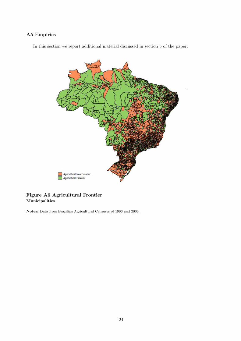
A5 Empirics
In this section we report additional material discussed in section 5 of the paper.
Figure A6 Agricultural FrontierMunicipalities
Notes: Data from Brazilian Agricultural Censuses of 1996 and 2006.
24

A6 Robustness Checks
A6.1 Additional Controls
Table A1 The effect of technological change on agricultureRobustness to controlling for additional initial municipality characteristics
(1) (2) (3) (4) (5) (6)PANEL A ∆ Soy area ∆ Maize area
∆Asoy 0.012*** 0.013*** 0.011*** -0.000 0.001 -0.002(0.002) (0.002) (0.002) (0.003) (0.003) (0.003)
∆Amaize -0.000 -0.001 -0.000 0.003*** 0.003** 0.004***(0.001) (0.001) (0.001) (0.001) (0.001) (0.001)
Log Agri Labor Prod 1985 0.001 -0.001(0.001) (0.002)
Log Avg Agri Wage 1991 -0.003** -0.008***(0.002) (0.003)
Agri Employment Share 1991 0.023*** 0.012(0.006) (0.009)
Baseline controls Yes Yes Yes Yes Yes Yes
Observations 3,841 3,683 3,841 4,032 3,872 4,032R-squared 0.118 0.117 0.121 0.015 0.015 0.015
(1) (2) (3) (4) (5) (6) (7) (8) (9)PANEL B ∆ Log output per worker 2006−1996 ∆ Log labor intensity 2006−1996 ∆ Employment share 2010−2000
∆Asoy 0.171*** 0.128*** 0.124*** -0.092*** -0.061*** -0.069*** -0.016*** -0.021*** -0.011***(0.028) (0.026) (0.027) (0.022) (0.021) (0.021) (0.003) (0.002) (0.002)
∆Amaize -0.046*** -0.034*** -0.031*** 0.042*** 0.031*** 0.035*** 0.004*** 0.006*** 0.003***(0.012) (0.012) (0.012) (0.009) (0.009) (0.009) (0.001) (0.001) (0.001)
Log Agri Labor Prod 1985/1996 -0.067*** 0.048*** -0.008***(0.020) (0.018) (0.002)
Log Avg Agri Wage 1991 -0.004 -0.041 -0.003(0.032) (0.028) (0.003)
Agri Employment Share 1991 0.114 0.095 -0.164***(0.115) (0.090) (0.011)
Baseline controls Yes Yes Yes Yes Yes Yes Yes Yes Yes
Observations 4,149 3,985 4,149 4,149 3,985 4,149 4,149 3,985 4,149R-squared 0.015 0.013 0.012 0.010 0.008 0.007 0.079 0.071 0.128
Notes: Changes calculated over the years 1996 and 2006 when the data sources are the Agricultural Censuses of 1996 and 2006, and over the years 2000 and 2010 when the datasources are the Population Censuses of 2000 and 2010. In Panel B: Log Agricultural Labor Productivity is from the 1985 Agricultural Census in columns 1 to 3 and from the 1996Agricultural Census in columns 4 to 9. The unit of observation is the AMC. Robust standard errors reported in parentheses. Significance levels: *** p<0.01, ** p<0.05, * p<0.1.
25
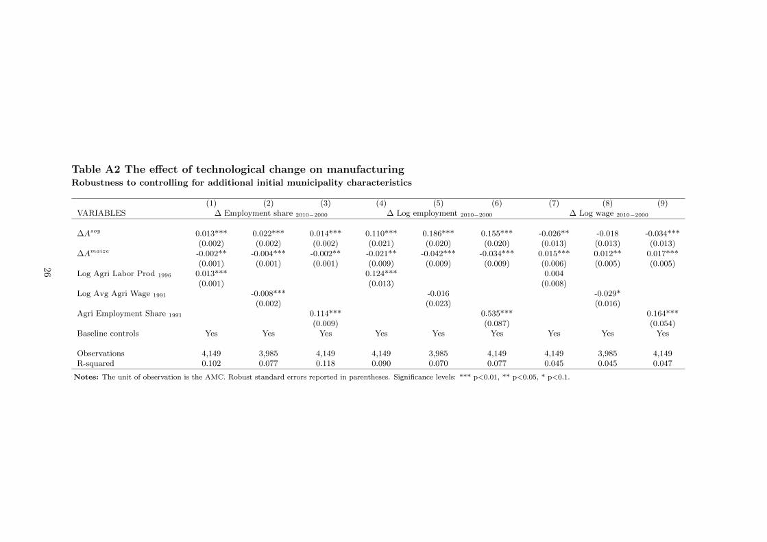
Table A2 The effect of technological change on manufacturingRobustness to controlling for additional initial municipality characteristics
(1) (2) (3) (4) (5) (6) (7) (8) (9)VARIABLES ∆ Employment share 2010−2000 ∆ Log employment 2010−2000 ∆ Log wage 2010−2000
∆Asoy 0.013*** 0.022*** 0.014*** 0.110*** 0.186*** 0.155*** -0.026** -0.018 -0.034***(0.002) (0.002) (0.002) (0.021) (0.020) (0.020) (0.013) (0.013) (0.013)
∆Amaize -0.002** -0.004*** -0.002** -0.021** -0.042*** -0.034*** 0.015*** 0.012** 0.017***(0.001) (0.001) (0.001) (0.009) (0.009) (0.009) (0.006) (0.005) (0.005)
Log Agri Labor Prod 1996 0.013*** 0.124*** 0.004(0.001) (0.013) (0.008)
Log Avg Agri Wage 1991 -0.008*** -0.016 -0.029*(0.002) (0.023) (0.016)
Agri Employment Share 1991 0.114*** 0.535*** 0.164***(0.009) (0.087) (0.054)
Baseline controls Yes Yes Yes Yes Yes Yes Yes Yes Yes
Observations 4,149 3,985 4,149 4,149 3,985 4,149 4,149 3,985 4,149R-squared 0.102 0.077 0.118 0.090 0.070 0.077 0.045 0.045 0.047
Notes: The unit of observation is the AMC. Robust standard errors reported in parentheses. Significance levels: *** p<0.01, ** p<0.05, * p<0.1.
26
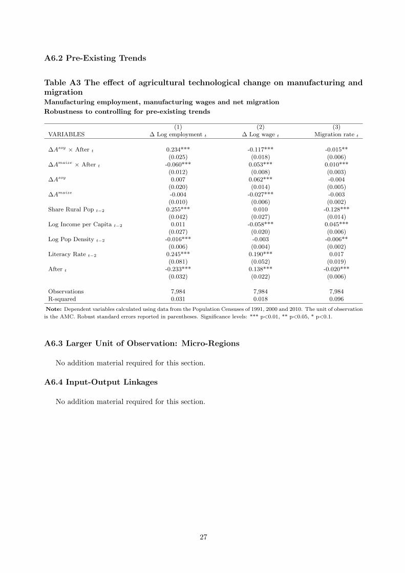
A6.2 Pre-Existing Trends
Table A3 The effect of agricultural technological change on manufacturing andmigrationManufacturing employment, manufacturing wages and net migration
Robustness to controlling for pre-existing trends
(1) (2) (3)VARIABLES ∆ Log employment t ∆ Log wage t Migration rate t
∆Asoy × After t 0.234*** -0.117*** -0.015**(0.025) (0.018) (0.006)
∆Amaize × After t -0.060*** 0.053*** 0.010***(0.012) (0.008) (0.003)
∆Asoy 0.007 0.062*** -0.004(0.020) (0.014) (0.005)
∆Amaize -0.004 -0.027*** -0.003(0.010) (0.006) (0.002)
Share Rural Pop t−2 0.255*** 0.010 -0.128***(0.042) (0.027) (0.014)
Log Income per Capita t−2 0.011 -0.058*** 0.045***(0.027) (0.020) (0.006)
Log Pop Density t−2 -0.016*** -0.003 -0.006**(0.006) (0.004) (0.002)
Literacy Rate t−2 0.245*** 0.190*** 0.017(0.081) (0.052) (0.019)
After t -0.233*** 0.138*** -0.020***(0.032) (0.022) (0.006)
Observations 7,984 7,984 7,984R-squared 0.031 0.018 0.096
Note: Dependent variables calculated using data from the Population Censuses of 1991, 2000 and 2010. The unit of observation
is the AMC. Robust standard errors reported in parentheses. Significance levels: *** p<0.01, ** p<0.05, * p<0.1.
A6.3 Larger Unit of Observation: Micro-Regions
No addition material required for this section.
A6.4 Input-Output Linkages
No addition material required for this section.
27

A6.5 Commodity Prices
100
200
300
400
500
Soy
bean
s, 2
000
US
$ pe
r m
etric
ton
1990
1992
1994
1996
1998
2000
2002
2004
2006
2008
2010
2012
2014
time
Figure A7 Evolution of soy price (1990-2013)
Notes: The Figure shows the monthly evolution of soy real price between 1990
and 2013. Data are from the IMF Primary Commodity Prices database, series
code: PSOYB USD, expressed in nominal US$ per metric ton. We deflate the
series using the US Consumer Price Index for All Urban Consumers: All Items,
source: Federal Reserve St. Louis, series code: CPIAUCNS, rescaled so that
2000 is the base year.50
100
150
200
250
Mai
ze, 2
000
US
$ pe
r m
etric
ton
1990
1992
1994
1996
1998
2000
2002
2004
2006
2008
2010
2012
2014
time
Figure A8 Evolution of maize price (1990-2013)
Notes: The Figure shows the monthly evolution of maize real price between 1990
and 2013. Data are from the IMF Primary Commodity Prices database, series
code: PMAIZMT US, expressed in nominal US$ per metric ton. We deflate the
series using the US Consumer Price Index for All Urban Consumers: All Items,
source: Federal Reserve St. Louis, series code: CPIAUCNS, rescaled so that
2000 is the base year.
28

Table A4 The effect of agricultural technological change on manufacturingData on employment and wages from the Annual Manufacturing Survey (PIA)
Robustness of results reported in Table 9 to controlling for commodity prices
(1) (2) (3) (4) (5) (6)VARIABLES Log Total Employment t Log Wage t
Asoy 0.122*** 0.122*** 0.096*** -0.026* -0.026* -0.018(0.030) (0.030) (0.029) (0.013) (0.013) (0.013)
Amaize -0.031** -0.031** -0.027* 0.013** 0.013** 0.011*(0.015) (0.015) (0.015) (0.006) (0.006) (0.006)
Share Rural Pop 1991 × t 0.052*** 0.052*** 0.019 0.030*** 0.030*** 0.025***(0.012) (0.012) (0.016) (0.005) (0.005) (0.007)
P soyAsoy -0.001 -0.000 0.000 0.000(0.001) (0.001) (0.001) (0.001)
PmaizeAmaize -0.001 -0.001 0.000 0.000(0.001) (0.001) (0.000) (0.000)
Literacy Rate 1991 × t -0.098*** 0.014(0.037) (0.017)
Log Pop Density 1991 × t -0.010*** 0.001(0.002) (0.001)
Log Income per Capita 1991 × t 0.019* -0.009**(0.010) (0.004)
Observations 25,262 25,262 25,262 25,239 25,239 25,239R-squared 0.923 0.923 0.923 0.778 0.778 0.778
Notes: Asoy is defined as potential soy yield under high inputs for the years between 2003 and 2007, and the potential soy yield under low inputs for the years between 1996 and
2002. Amaize is defined as potential maize yield under high inputs for the years between 2003 and 2007, and potential maize yield under low inputs for the years between 1996 and
2002. P zAz controls stand for the interaction of the potential yield of soy and maize under low inputs interacted with price levels of these crops between 1996 and 2007. The unit of
observation is the AMC. Standard errors clustered at AMC level reported in parentheses. Significance levels: *** p<0.01, ** p<0.05, * p<0.1.
29
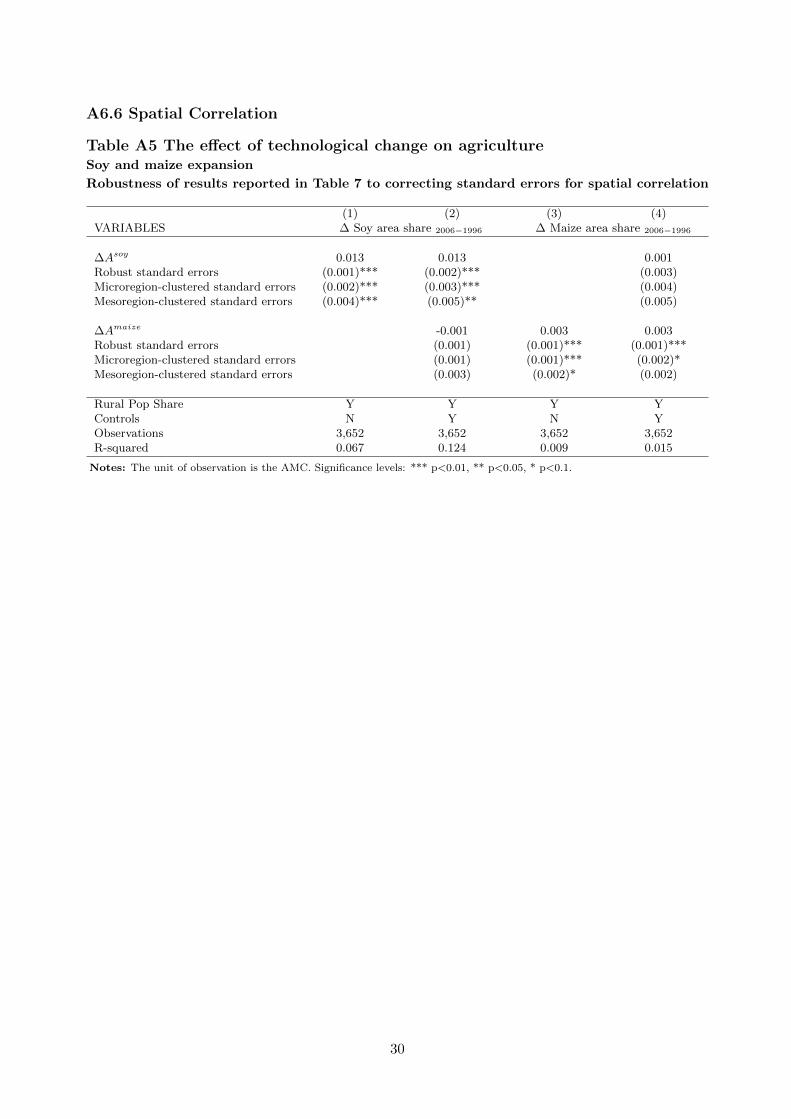
A6.6 Spatial Correlation
Table A5 The effect of technological change on agricultureSoy and maize expansion
Robustness of results reported in Table 7 to correcting standard errors for spatial correlation
(1) (2) (3) (4)VARIABLES ∆ Soy area share 2006−1996 ∆ Maize area share 2006−1996
∆Asoy 0.013 0.013 0.001Robust standard errors (0.001)*** (0.002)*** (0.003)Microregion-clustered standard errors (0.002)*** (0.003)*** (0.004)Mesoregion-clustered standard errors (0.004)*** (0.005)** (0.005)
∆Amaize -0.001 0.003 0.003Robust standard errors (0.001) (0.001)*** (0.001)***Microregion-clustered standard errors (0.001) (0.001)*** (0.002)*Mesoregion-clustered standard errors (0.003) (0.002)* (0.002)
Rural Pop Share Y Y Y YControls N Y N YObservations 3,652 3,652 3,652 3,652R-squared 0.067 0.124 0.009 0.015
Notes: The unit of observation is the AMC. Significance levels: *** p<0.01, ** p<0.05, * p<0.1.
30

Table A6 The effect of technological change on agricultureProductivity, labor intensity and employment share
Robustness of results reported in Table 8 to correcting standard errors for spatial correlation
(1) (2) (3)∆ Log output ∆ Log labor ∆ Employment
VARIABLES per worker 2006−1996 intensity 2006−1996 share 2010−2000
∆Asoy 0.131 -0.064 -0.021Robust standard errors (0.026)*** (0.021)*** (0.002)***Microregion-clustered standard errors (0.032)*** (0.026)** (0.004)***Mesoregion-clustered standard errors (0.033)*** (0.030)** (0.006)***
∆Amaize -0.033 0.033 0.006Robust standard errors (0.011)*** (0.009)*** (0.001)***Microregion-clustered standard errors (0.015)** (0.012)*** (0.002)***Mesoregion-clustered standard errors (0.016)** (0.015)** (0.003)*
Controls Y Y YObservations 4,149 4,149 4,149R-squared 0.012 0.007 0.073
Notes: The unit of observation is the AMC. Significance levels: *** p<0.01, ** p<0.05, * p<0.1.
Table A7 The effect of technological change on manufacturingEmployment share, employment and wages
Robustness of results reported in Table 9 to correcting standard errors for spatial correlation
(1) (2) (3)VARIABLES ∆ Employment share 2010 ∆ Log employment 2010 ∆ Log wage 2010
∆Asoy 0.021 0.186 -0.024Robust standard errors (0.002)*** (0.020)*** (0.012)*Microregion-clustered standard errors (0.004)*** (0.030)*** (0.014)*Mesoregion-clustered standard errors (0.006)*** (0.045)*** (0.019)
∆Amaize -0.004 -0.043 0.014Robust standard errors (0.001)*** (0.009)*** (0.005)**Microregion-clustered standard errors (0.002)** (0.014)*** (0.006)**Mesoregion-clustered standard errors (0.003) (0.027) (0.008)*
Controls Y Y YObservations 4,149 4,149 4,149R-squared 0.073 0.068 0.045
Notes: The unit of observation is the AMC. Significance levels: *** p<0.01, ** p<0.05, * p<0.1.
31

A6.7 Alternative Definition of Technical Change
Table A8 The effect of technological change on agriculture and manufacturingsRobustness to Alternative Definition of Technical Change
Agricultural outcomes Manufacturing outcomes∆ Soy area ∆ Maize area ∆ Log output per ∆ Log labor ∆ Employment ∆ Employment ∆ Log empl. ∆ Log wage
VARIABLES share 2006−1996 share 2006−1996 worker 2006−1996 intensity 2006−1996 share 2010−2000 share 2010−2000 2010−2000 2010−2000
∆ A soy (h−m) 0.020*** 0.002 0.163*** -0.145*** -0.019*** 0.014*** 0.155*** -0.040**(0.003) (0.004) (0.036) (0.029) (0.003) (0.003) (0.028) (0.016)
∆ A maize (h−m) -0.001 0.004** -0.043** 0.063*** 0.005*** -0.001 -0.030** 0.023***(0.001) (0.002) (0.017) (0.013) (0.002) (0.001) (0.014) (0.008)
Share Rural Pop 1991 0.038*** 0.010 0.090 -0.179*** -0.069*** 0.002 -0.017 -0.010(0.005) (0.007) (0.069) (0.050) (0.007) (0.005) (0.056) (0.034)
Log Income p.c. 1991 -0.000 -0.005 -0.007 0.040 0.012*** 0.004 0.111*** -0.106***(0.002) (0.004) (0.045) (0.038) (0.004) (0.003) (0.037) (0.026)
Log Pop Density 1991 -0.001*** 0.004*** -0.016 -0.019* 0.000 0.001 0.015* -0.035***(0.001) (0.001) (0.011) (0.010) (0.001) (0.001) (0.008) (0.005)
Literacy Rate 1991 0.056*** -0.009 -0.321** -0.088 -0.007 0.030*** 0.150 0.100(0.006) (0.012) (0.140) (0.116) (0.014) (0.010) (0.119) (0.075)
Observations 3,652 3,652 4,149 4,149 4,149 4,149 4,149 4,149R-squared 0.150 0.015 0.011 0.011 0.064 0.050 0.056 0.045
Notes: ∆Asoy (h−m) is defined as potential soy yield under high inputs minus potential soy yield under intermediate level of inputs. ∆Amaize (h−m) is defined as potential maize
yield under high inputs minus potential maize yield under intermediate level of inputs. Changes calculated over the years 1996 and 2006 when the data sources are the Agricultural
Censuses of 1996 and 2006, and over the years 2000 and 2010 when the data sources are the Population Censuses of 2000 and 2010. The unit of observation is the AMC. Robust
standard errors reported in parentheses. Significance levels: p<0.01, p<0.05, p<0.1.
32
References
CONAB (2003-2012). “Levantamento De Avaliacao Da Safra”.
Herrendorf, B., R. Rogerson, and A. Valentinyi (2013). “Two Perspectives on Preferences and
Structural Transformation”. American Economic Review 103 (7), 2752–2789.
IBGE (1996). “Censo Agropecuario 1995-1996”. Rio de Janeiro, Brazil: Instituto Brasileiro de
Geografia e Estatıstica (IBGE).
IBGE (2003). “Metodologia do Censo Demografico”, Volume 25. Rio de Janeiro, Brazil: Instituto
Brasileiro de Geografia e Estatıstica (IBGE).
IBGE (2006). “Censo Agropecuario 2006”. Rio de Janeiro, Brazil: Instituto Brasileiro de Geografia
e Estatıstica (IBGE).
Shryock, H. S., J. S. Siegel, and E. A. Larmon (1980). The methods and materials of demography,
Volume 2. Department of Commerce, Bureau of the Census.
33