Embed Size (px)
Citation preview
TelecommunicationsMicrowave
Microwave Fundamentals
Courseware Sample 85756-F0

Order no.: 85756-00
Second Edition
Revision level: 03/2015
By the staff of Festo Didactic
© Festo Didactic Ltée/Ltd, Quebec, Canada 2008, 2009
Internet: www.festo-didactic.com
e-mail: [email protected]
Printed in Canada
All rights reserved
ISBN 978-2-89640-345-5 (Printed version)
ISBN 978-2-89747-377-8 (CD-ROM)
Legal Deposit – Bibliothèque et Archives nationales du Québec, 2009
Legal Deposit – Library and Archives Canada, 2009
The purchaser shall receive a single right of use which is non-exclusive, non-time-limited and limited
geographically to use at the purchaser's site/location as follows.
The purchaser shall be entitled to use the work to train his/her staff at the purchaser's site/location and
shall also be entitled to use parts of the copyright material as the basis for the production of his/her own
training documentation for the training of his/her staff at the purchaser's site/location with
acknowledgement of source and to make copies for this purpose. In the case of schools/technical
colleges, training centers, and universities, the right of use shall also include use by school and college
students and trainees at the purchaser's site/location for teaching purposes.
The right of use shall in all cases exclude the right to publish the copyright material or to make this
available for use on intranet, Internet and LMS platforms and databases such as Moodle, which allow
access by a wide variety of users, including those outside of the purchaser's site/location.
Entitlement to other rights relating to reproductions, copies, adaptations, translations, microfilming and
transfer to and storage and processing in electronic systems, no matter whether in whole or in part, shall
require the prior consent of Festo Didactic GmbH & Co. KG.
Information in this document is subject to change without notice and does not represent a commitment on
the part of Festo Didactic. The Festo materials described in this document are furnished under a license
agreement or a nondisclosure agreement.
Festo Didactic recognizes product names as trademarks or registered trademarks of their respective
holders.
All other trademarks are the property of their respective owners. Other trademarks and trade names may
be used in this document to refer to either the entity claiming the marks and names or their products.
Festo Didactic disclaims any proprietary interest in trademarks and trade names other than its own.

© Festo Didactic 85756-00 III
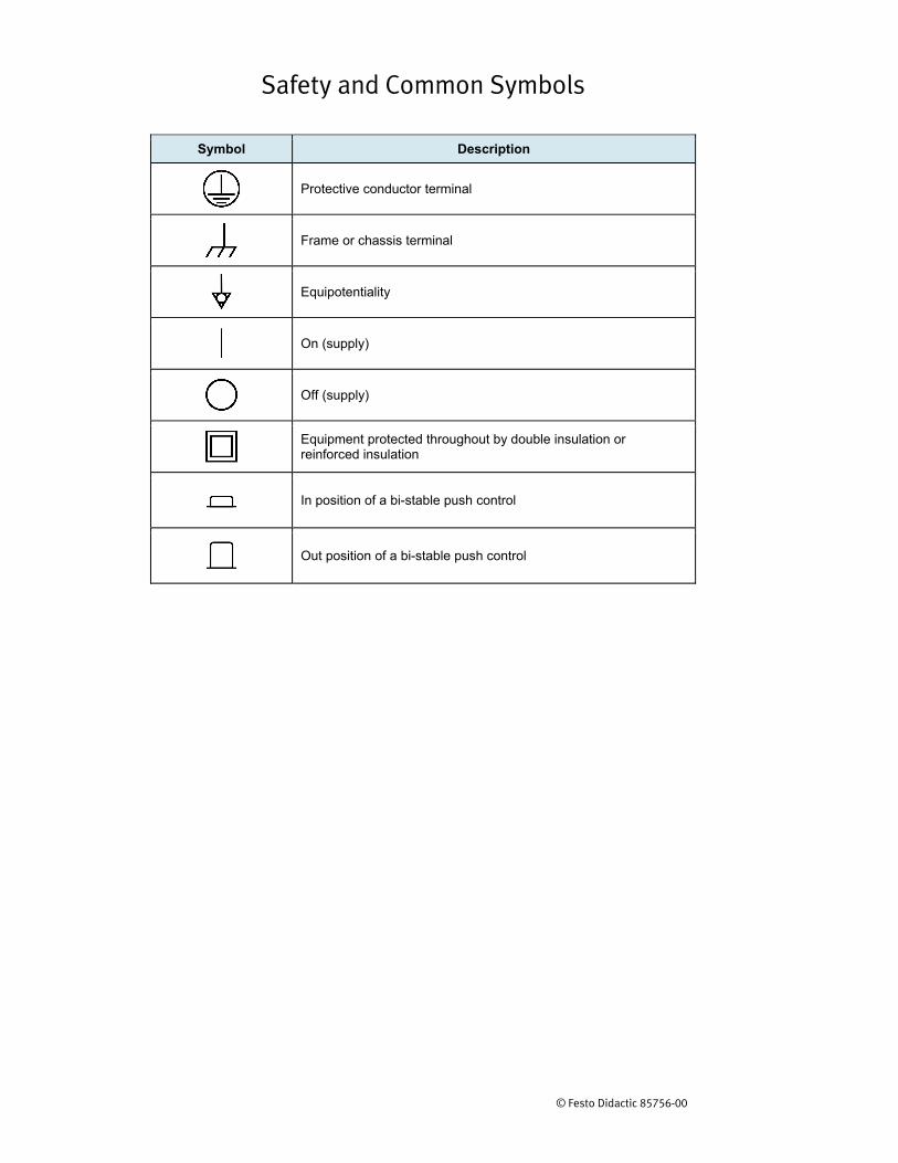
Safety and Common Symbols
The following safety and common symbols may be used in this manual and on the equipment:
Symbol Description
DANGER indicates a hazard with a high level of risk which, if not avoided, will result in death or serious injury.
WARNING indicates a hazard with a medium level of risk which, if not avoided, could result in death or serious injury.
CAUTION indicates a hazard with a low level of risk which, if not avoided, could result in minor or moderate injury.
CAUTION used without the Caution, risk of danger sign , indicates a hazard with a potentially hazardous situation which, if not avoided, may result in property damage.
Caution, risk of electric shock
Caution, hot surface
Caution, risk of danger
Caution, lifting hazard
Caution, hand entanglement hazard
Notice, non-ionizing radiation
Direct current
Alternating current
Both direct and alternating current
Three-phase alternating current
Earth (ground) terminal
Safety and Common Symbols
© Festo Didactic 85756-00
Symbol Description
Protective conductor terminal
Frame or chassis terminal
Equipotentiality
On (supply)
Off (supply)
Equipment protected throughout by double insulation or reinforced insulation
In position of a bi-stable push control
Out position of a bi-stable push control
© Festo Didactic 85756-00 V
Table of Contents
Preface ................................................................................................................ XV
About This Manual ............................................................................................ XVII
Exercise 1 Familiarization with Microwave Equipment ............................... 1
DISCUSSION ...................................................................................... 1 Guided propagation of microwaves .......................................... 1 Basic components of the Microwave Technology Training System ...................................................................................... 2
The Gunn Oscillator .................................................................... 2 The Gunn Oscillator Power Supply .......................................... 2 The Variable Attenuator ........................................................... 3 The Thermistor Mount .............................................................. 4 Assembly of components ......................................................... 5 Using the Power Meter of the LVDAM-MW software ............... 7
PROCEDURE ..................................................................................... 8 Set up and connections ............................................................ 8
Exercise 2 Power Measurements ................................................................. 15
DISCUSSION .................................................................................... 15 Power ..................................................................................... 15 Watt and decibel conversion .................................................. 16 Power measurement techniques ............................................ 17 Wheatstone bridge ................................................................. 18
Bridge balancing ....................................................................... 19 Bridge operation ....................................................................... 19
PROCEDURE ................................................................................... 20 Set up and connections .......................................................... 20 Measuring the power fed to the thermistor at equilibrium, without microwave signal injected .......................................... 23 Measuring the power fed to the thermistor at equilibrium, when a microwave signal is injected ...................................... 23
Exercise 3 The Gunn Oscillator.................................................................... 27
DISCUSSION .................................................................................... 27 Introduction to Gunn oscillators .............................................. 27 The Gunn effect ...................................................................... 27 Current-voltage characteristic of a Gunn diode...................... 28
Energy levels of n-type semiconductor materials ...................... 29 Creation of microwave oscillations ............................................ 29 Natural frequency of the created oscillation .............................. 30
Turning a Gunn diode into a Gunn oscillator .......................... 30
Table of Contents
© Festo Didactic 85756-00
PROCEDURE ................................................................................... 31 Measuring the current, power, and efficiency of the Gunn Oscillator over the 0-10 V supply voltage range .................... 31 Plotting the current-versus-voltage curve of the Gunn Oscillator ................................................................................. 35 Plotting the power-versus-voltage curve and the efficiency-versus-voltage curve of the Gunn Oscillator .......... 36
Exercise 4 Calibration of the Variable Attenuator ...................................... 39
DISCUSSION .................................................................................... 39 Attenuation ............................................................................. 39 Insertion loss .......................................................................... 40 Techniques used to measure attenuation and its insertion losses ..................................................................................... 42
PROCEDURE ................................................................................... 43 Measuring the maximum power fed to the load ..................... 43 Characterizing the Variable Attenuator by plotting its attenuation-versus-blade position curve ................................ 45
Exercise 5 Detection of Microwave Signals ................................................ 51
DISCUSSION .................................................................................... 51 Introduction to crystal detectors ............................................. 51 Typical sensitivity curve of a crystal detector ......................... 51 Voltage sensitivity ................................................................... 52 Amplification of a crystal detector's output signal .................. 52 Measuring the tangential sensitivity ....................................... 53
PROCEDURE ................................................................................... 54 Measuring the maximum power of the microwave signal ...... 54 Determining the sensitivity curve of the crystal detector ........ 56 Measuring the tangential sensitivity of the Crystal Detector .................................................................................. 62
Exercise 6 Attenuation Measurements ........................................................ 67
DISCUSSION .................................................................................... 67 The RF substitution method ................................................... 67 Advantages and limitations of the RF substitution method .... 68 The SWR Meter of LVDAM-MW ............................................. 68 Power and attenuation measurements .................................. 68
Steps to perform when starting the SWR Meter of LVDAM-
MW ............................................................................................ 69

Table of Contents
© Festo Didactic 85756-00 VII
PROCEDURE ................................................................................... 70 System setup .......................................................................... 70 SWR Meter preliminary adjustment ....................................... 72 Measuring the attenuation provided by a microwave component .............................................................................. 73
Exercise 7 Standing Waves .......................................................................... 77
DISCUSSION .................................................................................... 77 Creation of standing waves .................................................... 77 Conventional representation of standing waves .................... 78 Frequency measurement ....................................................... 79 The Slotted Line ..................................................................... 80 Microwave frequency measurements and standing wave measurements ........................................................................ 81 Start-up procedure when using the Slotted Line and the SWR Meter of LVDAM-MW .................................................... 82
PROCEDURE ................................................................................... 83 System setup .......................................................................... 83
Preliminary adjustment of the Slotted Line and SWR Meter ..... 85 Measuring the guided wavelength and the microwave signal frequency ..................................................................... 88
Standing wave produced along the Slotted Line when the
waveguide is short-circuited ...................................................... 89 Standing wave produced along the Slotted Line when the load consists of a 6 dB attenuator and a short circuit ............ 92 Standing wave produced along the Slotted Line with a matched load .......................................................................... 97
Exercise 8 The Directional Coupler ........................................................... 103
DISCUSSION .................................................................................. 103 Introduction to directional couplers ...................................... 103 Construction and operation of a cross-guide directional coupler .................................................................................. 103 Electric and magnetic field distributions inside a waveguide ............................................................................ 105
Orientation of the components of the magnetic field in a
cross-guide directional coupler ............................................... 106 Coupling factor ..................................................................... 107 Directivity .............................................................................. 108
PROCEDURE ................................................................................. 109 System setup ........................................................................ 109
Setting the maximum power to 0 dBm on the Power Meter .... 109 Setting the reference on the SWR Meter ................................ 112
Measuring the coupling factor of the Directional Coupler .... 114 Measuring the directivity of the Directional Coupler ............. 116

Table of Contents
I © Festo Didactic 85756-00
Exercise 9 Reflection Coefficient Measurements ..................................... 119
DISCUSSION .................................................................................. 119 Reflection coefficient ............................................................ 119 Power incident to and reflected by a load ............................ 120 Return loss ........................................................................... 120 Percentage of the incident power absorbed by the load ...... 121 Measuring the reflection coefficient of a load ....................... 121
Vectorial voltmeter method ..................................................... 121 Reflectometer (dual power meter) method .............................. 121 Reflectometer square-law method .......................................... 122
PROCEDURE ................................................................................. 124 System setup ........................................................................ 124
Measuring the return loss and the magnitude of the
reflection coefficient ................................................................ 124 Return loss of the thermistor mount when it is matched and poorly matched .............................................................. 128
Matching the Thermistor Mount ............................................... 128 Setting the reference on the SWR Meter ................................ 130 Measuring the return loss of the matched Thermistor Mount .. 132
Exercise 10 SWR Measurements ................................................................. 137
DISCUSSION .................................................................................. 137 Standing wave ratio (SWR) .................................................. 137 SWR and magnitude of the reflection coefficient, ρ ............. 138 Converting SWR (dimensionless number) into dB ............... 139 SWR measurements with a Slotted Line and a SWR Meter .................................................................................... 139
PROCEDURE ................................................................................. 140 Measuring the SWR when the impedance of the load is matched to the impedance of the waveguide ....................... 140 Measuring the SWR when the load consists of an attenuator and a short circuit ................................................ 144
Decreasing the attenuation provided by the Variable
Attenuator ............................................................................... 146 Measuring the SWR when the load consists of a short circuit .................................................................................... 148
Exercise 11 Impedance Measurements ....................................................... 153
DISCUSSION .................................................................................. 153 Relationship between the reflection coefficient at the load and the load impedance ....................................................... 153 The Smith Chart ................................................................... 154
Circles of constant resistance (R) value .................................. 156 Arcs of constant reactance (± jX/Z0) values ............................ 158

Table of Contents
© Festo Didactic 85756-00 IX
Plotting a normalized impedance on the Smith Chart .......... 160 Determining the SWR produced by a given load ................. 162 Determining the magnitude (ρ) and phase angle (φ) of the reflection coefficient produced by a given load .................... 164 Determining the impedance of a load with a Slotted Line (short-circuit minima-shift method) ....................................... 166
PROCEDURE ................................................................................. 169 Determining the guided wavelength with the Slotted Line ... 169 Measuring the load impedance by using the short-circuit minima-shift method ............................................................. 173
Measuring the load impedance with the Variable Attenuator
set for an attenuation of 5.0 dB ............................................... 173 Measuring the load impedance with the Variable Attenuator
set for an attenuation of 1.5 dB ............................................... 176
Exercise 12 Reactive Impedances ............................................................... 181
DISCUSSION .................................................................................. 181 Discontinuity ......................................................................... 181 Capacitive and inductive irises ............................................. 182 The screw tuner .................................................................... 183 Determining the reactance produced by an iris or a screw tuner in a waveguide ............................................................ 184 Converting impedances to admittances by using the Smith Chart .......................................................................... 185 Converting admittances to impedances by using the Smith Chart .......................................................................... 187 Determining the admittance and the impedance of an iris by using the Smith Chart ...................................................... 187
PROCEDURE ................................................................................. 190 Determining the location of the phase reference plane ....... 190 Determining the admittance and the impedance of an inductive iris by using a Smith Chart .................................... 193
Determining the reflection coefficient in the plane of the iris ... 195 Determining the normalized total impedance and the
normalized total admittance in the plane of the iris ................. 196 Determining the normalized admittance and the normalized
impedance of the iris ............................................................... 198
Exercise 13 Impedance Matching ................................................................ 203
DISCUSSION .................................................................................. 203 Reflection coefficient along a waveguide ............................. 203 Determining an impedance along a waveguide ................... 203
Determining the impedance at a given point along a
waveguide (example) .............................................................. 206

Table of Contents
© Festo Didactic 85756-00
Impedance matching ............................................................ 208 Impedance matching of a load (example) ............................... 209
Slide-Screw Tuner ................................................................ 211
PROCEDURE ................................................................................. 212 Determining the location of the phase reference plane ....... 212 Measuring the impedance of an unmatched load ................ 216 Adjusting the slide-screw tuner to match the load................ 219 Measuring the SWR of the matched load ............................ 222 Determining the impedance and the location of the matching device (Slide-Screw Tuner) required to match the load ................................................................................. 224
Exercise 14 Antennas and Propagation ...................................................... 229
DISCUSSION .................................................................................. 229 Propagation in free space .................................................... 229 Propagation loss ................................................................... 230 Isotropic radiators ................................................................. 230
Measuring the attenuation ....................................................... 230 Transmission and reception of signals ................................. 231 Radiation pattern .................................................................. 231 Plotting a radiation pattern ................................................... 232 Methods used to measure the gain of an antenna ............... 234
Reference-antenna gain measurement method ...................... 234 Identical-antenna gain measurement method ......................... 234
PROCEDURE ................................................................................. 235 Measuring the received signal level for various distances between the transmitting and receiving antennas ................ 235 Measuring the gain of an antenna ........................................ 240 Plotting and comparing the radiation patterns of two different antennas ................................................................. 244
Plotting the radiation pattern of a horn antenna ...................... 244 Plotting the radiation pattern of a long triangular lens
antenna ................................................................................... 247
Exercise 15 Microwave Optics ..................................................................... 255
DISCUSSION .................................................................................. 255 Phenomena usually encountered in optics .......................... 255 Index of refraction ................................................................. 255 Reflection coefficient ............................................................ 256 Coefficient of transmission ................................................... 257 Snell's Law ........................................................................... 257
Critical angle ........................................................................... 258 Lenses .................................................................................. 258 Parabolic antennas ............................................................... 259

Table of Contents
© Festo Didactic 85756-00 XI
PROCEDURE ................................................................................. 260 Interference caused by a metal plate ................................... 260 Observing the effect that a change in the plate orientation has on the level of the received signal ................................. 264
With the metal plate ................................................................ 264 With the dielectric plate ........................................................... 265
Comparing the signal levels received with the two plates .... 266
Exercise 16 Microwave Transmission Demonstration (Requires Optional Equipment)................................................................. 269
DISCUSSION .................................................................................. 269 Microwave transmission demonstration ............................... 269
PROCEDURE ................................................................................. 272 System setup and adjustment of the operating point ........... 272 Observations related to the propagation of microwave signals with and without obstacles ....................................... 277 Observations related to the polarization of the wave ........... 280 Transmission of an audio signal ........................................... 282
Exercise 17 PIN Diodes ................................................................................. 287
DISCUSSION .................................................................................. 287 Introduction ........................................................................... 287 Operation of a PIN diode when forward-biased ................... 288 Typical resistance-versus-bias current response of a forward-biased PIN diode ..................................................... 288 Equivalent RF circuit of a forward-biased PIN diode ........... 289 Operation of a PIN diode when reverse-biased ................... 291 Attenuation of a reverse-biased PIN diode as a function of frequency .............................................................................. 292 Applications of PIN diodes ................................................... 293
PROCEDURE ................................................................................. 294 Characterization of the PIN Diode ........................................ 294 PIN diode used as a microwave switch ................................ 302 Attenuation-versus-frequency curve of the PIN diode (optional section) .................................................................. 306
Exercise 18 Wireless Video Transmission System (Requires Optional Equipment) ................................................................................ 313
DISCUSSION .................................................................................. 313 Introduction ........................................................................... 313 Constructive and destructive interference: multipath interference .......................................................................... 315
Table of Contents
© Festo Didactic 85756-00
PROCEDURE ................................................................................. 315 Characterization of the PIN diode ........................................ 315 Constructive and destructive interference ............................ 319 E-plane attenuation .............................................................. 320
Exercise 19 Hybrid Tees ............................................................................... 325
DISCUSSION .................................................................................. 325 Introduction to waveguide tees............................................. 325 The hybrid (magic) tee ......................................................... 326 Using hybrid tees to split signals .......................................... 327
Theoretical versus actual attenuation and isolation ................. 328 Using hybrid tees to couple signals ...................................... 328 Applications .......................................................................... 329
PROCEDURE ................................................................................. 331 System setup ........................................................................ 331
Setting the maximum power to 0 dBm .................................... 331 Setting the reference on the SWR meter ................................ 334
Attenuation between the H-plane arm and lateral arm 1 ..... 336 Attenuation between the H-plane arm and lateral arm 2 ..... 338 Attenuation between the E-plane arm and lateral arm 1 ...... 340 Attenuation between the E-plane arm and lateral arm 2 ...... 341 Measuring the isolation between the E- and H-plane arms of the hybrid tee .................................................................... 343
Isolation between the E-plane arm and the H-plane arm
(E➞H) ..................................................................................... 343 Isolation between the H-plane arm and the E-plane arm
(H➞E) ..................................................................................... 345 180° phase difference verification ........................................ 346
Signal propagation with short-circuit termination at lateral
port 1 ....................................................................................... 346 Signal propagation with short-circuit termination at lateral
port 2 ....................................................................................... 348 180° phase difference verification ........................................ 349 Calculating the reflection loss from the measured SWR ...... 351
Appendix A Equipment Utilization Chart ..................................................... 357
Appendix B Glossary of New Terms ............................................................ 359
Appendix C Common Symbols .................................................................... 361
Appendix D Module Front Panels ................................................................. 367

Table of Contents
© Festo Didactic 85756-00 XIII
Appendix E Answers to Procedure Step Questions .................................. 369 Exercise 1 ............................................................................. 369 Exercise 2 ............................................................................. 369 Exercise 3 ............................................................................. 370 Exercise 4 ............................................................................. 371 Exercise 5 ............................................................................. 371 Exercise 6 ............................................................................. 372 Exercise 7 ............................................................................. 373 Exercise 8 ............................................................................. 377 Exercise 9 ............................................................................. 377 Exercise 10 ........................................................................... 378 Exercise 11 ........................................................................... 379 Exercise 12 ........................................................................... 380 Exercise 13 ........................................................................... 381 Exercise 14 ........................................................................... 383 Exercise 15 ........................................................................... 388 Exercise 16 ........................................................................... 389 Exercise 17 ........................................................................... 391 Exercise 18 ........................................................................... 393 Exercise 19 ........................................................................... 393
Appendix F Answers to Review Questions ................................................ 397 Exercise 1 ............................................................................. 397 Exercise 2 ............................................................................. 397 Exercise 3 ............................................................................. 398 Exercise 4 ............................................................................. 399 Exercise 5 ............................................................................. 399 Exercise 6 ............................................................................. 400 Exercise 7 ............................................................................. 401 Exercise 8 ............................................................................. 401 Exercise 9 ............................................................................. 402 Exercise 10 ........................................................................... 403 Exercise 11 ........................................................................... 404 Exercise 12 ........................................................................... 405 Exercise 13 ........................................................................... 408 Exercise 14 ........................................................................... 408 Exercise 15 ........................................................................... 409 Exercise 16 ........................................................................... 409 Exercise 17 ........................................................................... 410 Exercise 18 ........................................................................... 411 Exercise 19 ........................................................................... 412
Appendix G Conversion Table ...................................................................... 415
Index of New Terms ........................................................................................... 417
Bibliography ....................................................................................................... 419

© Festo Didactic 85756-00 XV
Preface
Although the microwave field is relatively new, microwaves are now a part of our everyday life. Almost all of us have watched television programs transmitted across continents and oceans via microwave satellite links, cooked meals in a microwave oven, or been in an airplane using microwave radar to help it land in conditions of poor visibility. None of these things were possible only a few years ago, and even today, the full potential of microwaves has not been realized.
The first use of microwaves was in radar applications developed during World War II. Since then, interest in microwave technology has grown rapidly. Microwaves are now used in such applications as well as in air traffic control at airports throughout the world, navigational aids at sea and on land, and missile-tracking systems to name just a few. Microwaves have helped to increase the useable radio-frequency spectrum, and today, they play an important role in telecommunications. Earth-orbiting satellites are able to relay vast quantities of information over long distances in very short periods of time. Satellites have done much to "shrink" the world, making it possible to communicate with remote areas that are too isolated for conventional communications technology.
Microwaves offer so many varied applications, such as the microwave oven, which are just not possible with lower frequencies that one may wonder what it is about microwaves that makes them so different from other signals. The answer lies in the wavelength of signals at microwave frequencies. With wavelengths from about 0.1 to 100 cm, the microwave signal's wavelength is comparable to the size of the circuit components. Because of the shortness of the wavelength, the propagation time of electrical quantities is comparable to the period of the signal, and many phenomena can, therefore, occur in a relatively short distance. This makes it easy to observe such things as standing waves, and to measure the maxima and minima of the electric fields using compact devices with probes. Unlike lower-frequency signals, microwaves are able to penetrate the ionized layers of the ionosphere with a minimum of diffraction and reach satellites orbiting at heights equivalent to three times the Earth's diameter.
Progress in the field of microwaves has only been possible since higher-frequency microwave sources have been available. In the beginning, these sources were made from magnetrons and klystrons. Today, solid-state devices, such as the Gunn Effect oscillator, are available. With the high-frequency signals from these sources, it is possible to use very large bandwidths to transmit vast quantities of information.
This manual, Microwave Fundamentals, introduces students to the principles of microwave signals and their propagation; the construction and operation of microwave components; and the techniques used to measure power attenuation, SWR, and impedance.
All measurements are performed by using the Windows®-based Data Acquisition and Management for Microwave system (LVDAM-MW®). This software includes a power meter, a standing-wave ratio (SWR) meter, and an oscilloscope. The software allows the user to display, save, and print data and graphs. A Smith Chart is included to permit the measurements of the line parameters. The software is built around the Data Acquisition Interface (DAI), Model 9508, that performs 12-bit A/D acquisition on four channels.
The equipment required to perform the exercises in this manual is listed in Appendix A.

Preface
I © Festo Didactic 85756-00
Acknowledgments
We thank Mr. Gilles Ratté, MScA, of Comlab Inc. for his special contribution to this text. We would also like to thank the following people from Laval University, Québec, for their participation in the development of the Microwave Technology instructional program: John Ahern, MScA; Gilles Y. Delisle, PhD; Michel Lecours, PhD; Marcel Pelletier, PhD.
We invite readers of this manual to send us their tips, feedback, and suggestions for improving the book.
Please send these to [email protected].
The authors and Festo Didactic look forward to your comments.
© Festo Didactic 85756-00 XVII
About This Manual
The exercises in this manual provide a systematic introduction to the very wide microwave field. When students are first confronted with the components and devices of a microwave system, they are often disconcerted by their physical difference compared to those that they are familiar with. Therefore, it is very important not to overwhelm the students with a mass of new concepts, components, and techniques.
The approach used in this manual is simple and progressive. It uses a recognized pedagogic approach that introduces concepts, components, and measuring devices one at a time in a logical order. Each element introduced adds to the base on which the next element will be introduced. Thus, in this introductory manual, we introduce: fundamental quantities such as power, impedance, attenuation, standing waves, and reflection coefficients; components and measuring devices such as fixed and variable attenuators, crystal detectors, directional couplers, loads or terminations, reactive irises, SWR meters, and power meters; and techniques for measuring power, attenuation, standing-wave ratios, reflection coefficients, and impedance. Other associated topics such as impedance matching, antennas and microwave propagation, and microwave optics are also introduced.
Exercises 1 to 5 introduce the students to many of the basic components of the Microwave Technology Training System with LVDAM-MW, Model 8091, and some of the techniques which will be used throughout the manual. Exercise 6 familiarizes the student with the RF substitution method of measuring the attenuation caused by a microwave component. Exercise 7 introduces reflected and standing waves. The slotted line is introduced as a useful tool for studying the parameters of these phenomena. Exercise 8 introduces the directional coupler.
Exercise 9 covers the reflection coefficient and the return loss. Exercise 10 further familiarizes the students with standing waves and the measurement of standing-wave ratios.
Exercises 11 to 13 introduce students to the Smith Chart. The students learn how to measure reactive impedances. They learn how to perform impedance matching to reduce the reflection produced by mismatched load to a minimum.
Exercises 14 and 15 present more advanced concepts. In Exercise 14, the students learn how to measure the gain of a horn antenna, and how to plot radiation patterns. Exercise 15 introduces the students to microwave optics.
Exercise 16 teaches how to implement a simple demonstration to show how a microwave signal can be used to carry information along a line of sight from one point to another. Optional equipment is required (indicated in Appendix A).
Exercises 17 and 18 introduce students to the construction and operation of PIN diodes. The students learn how PIN diodes are used in microwave applications such as microwave switching, variable attenuation, amplitude modulation and leveling, and wireless communication systems. The students can implement and test a wireless video transmission system that uses a PIN diode as a microwave AM modulator. For this demonstration, option equipment is required (indicated in Appendix A).
About This Manual
III © Festo Didactic 85756-00
Exercise 19 explains the operation of hybrid (magic) tees and how they can split a microwave signal into two even signals, or couple two microwave signals into a single signal. Typical applications of hybrid tees are described.
Each exercise is designed as a small instructional segment. Principles and concepts are presented first. Then, hands-on procedures enhance the written material to involve and better acquaint the students with the material being covered. A five-question review is presented at the end of each exercise. These questions allow the student to verify that the material has been well assimilated.
Safety considerations
Safety symbols that may be used in this manual and on the equipment are listed in the Safety Symbols table at the beginning of the manual.
Safety procedures related to the tasks that you will be asked to perform are indicated in each exercise.
Make sure that you are wearing appropriate protective equipment when performing the tasks. You should never perform a task if you have any reason to think that a manipulation could be dangerous for you or your teammates.
Safety with RF Fields
When studying Microwave Systems, it is very important to develop good safety habits. Although microwaves are invisible, they can be dangerous at high levels or for long exposure times. The most important safety rule when working with microwave equipment is to avoid exposure to dangerous radiation levels.
The radiation levels in the 8091 Microwave Technology Training System are too low to be dangerous because it uses the Gunn Oscillator, Model 9510, which is a low-power source of microwave signal. The maximum power level of the Gunn Oscillator at a frequency of 10 GHz, which varies from one unit to another, ranges between 10 and 25 mW. In the worst case, i.e. at the aperture of the waveguide where the maximum power level is 25 mW, the maximum power density produced by the Microwave Technology Training System is approximately 3.0 mW/cm2. This low power density allows safe operation in a classroom laboratory.
In order to develop good safety habits, you should, whenever possible, remove the power from the Gunn Oscillator before placing yourself in front of the transmitting antenna. Your instructor may have additional safety directives for this system.
For your safety, do not look directly into the waveguides or Horn Antennas whilepower is being supplied to the Gunn Oscillator.
About This Manual
© Festo Didactic 85756-00 XIX
a Detailed information on how to set up and use the instruments of the LVDAM-MW software can be found in the User Guide "Microwave Data Acquisition and Management", Model 85756-E. Additional information on how to use these instruments can be found in the Help section of this software, accessible from the software main window. Information on the instruments used to control or monitor the PIN Diode and the Frequency Meter of the optional Voltage Controlled RF Oscillator (VCO), Model 9511, are provided in the Parameter Settings section of the Help.
Systems of units
Units are expressed using the International System of Units (SI) followed by the units expressed in the U.S. customary system of units (between parentheses).


Sample Exercise
Extracted from
Student Manual

© Festo Didactic 85756-00 77
When you have completed this exercise, you will know how standing waves are created in waveguides. You will be able to perform microwave frequency measurements and standing wave measurements with the Slotted Line and the SWR Meter of LVDAM-MW.
The Discussion of this exercise covers the following points:
Creation of standing waves Conventional representation of standing waves Frequency measurement The Slotted Line Microwave frequency measurements and standing wave measurements Start-up procedure when using the Slotted Line and the SWR Meter of
LVDAM-MW
Creation of standing waves
When a sinusoidal microwave source is connected to a waveguide, sinusoidal waves of voltage and current propagate along it.
a In fact, we could also say that both an electric field wave and a magnetic field wave propagate inside the waveguide. Considering voltages and currents instead of electric and magnetic fields is simply a different way of viewing things. The voltage is present between the top and the bottom of the waveguide, whereas the current flows in the side walls. Throughout this exercise, we will deal with voltages and currents to facilitate the understanding.
The amplitude of the voltage and the current depend on the characteristic impedance of the waveguide and on the impedance of the terminating load.
When the impedance of the load is equal to the characteristic impedance of the waveguide, the load continually absorbs all the received energy. No energy is reflected back toward the source. The waves travel only from the source to the load.
Conversely, when the impedance of the load is not equal to the characteristic impedance of the waveguide, not all the received energy is absorbed by the load. Instead, part of it is reflected back toward the source.
Standing Waves
Exercise 7
EXERCISE OBJECTIVE
DISCUSSION OUTLINE
DISCUSSION
Exercise 7 – Standing Waves Discussion
78 © Festo Didactic 85756-00
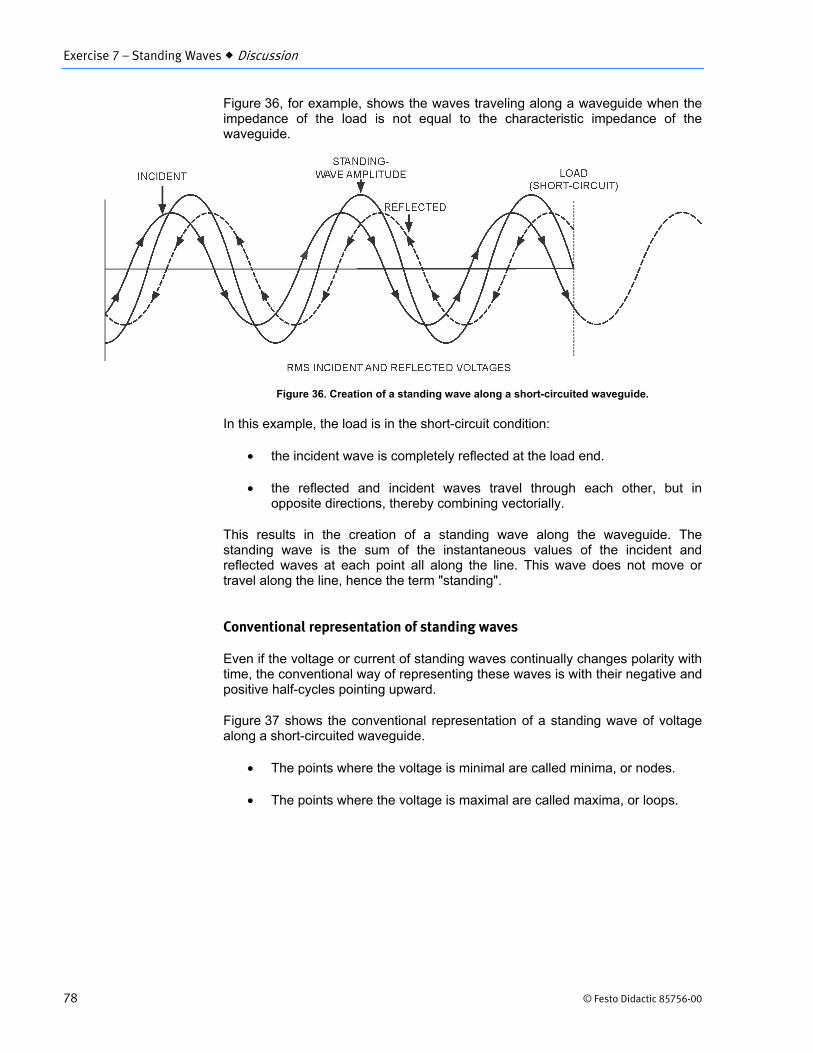
Figure 36, for example, shows the waves traveling along a waveguide when the impedance of the load is not equal to the characteristic impedance of the waveguide.
Figure 36. Creation of a standing wave along a short-circuited waveguide.
In this example, the load is in the short-circuit condition:
• the incident wave is completely reflected at the load end.
• the reflected and incident waves travel through each other, but in opposite directions, thereby combining vectorially.
This results in the creation of a standing wave along the waveguide. The standing wave is the sum of the instantaneous values of the incident and reflected waves at each point all along the line. This wave does not move or travel along the line, hence the term "standing".
Conventional representation of standing waves
Even if the voltage or current of standing waves continually changes polarity with time, the conventional way of representing these waves is with their negative and positive half-cycles pointing upward.
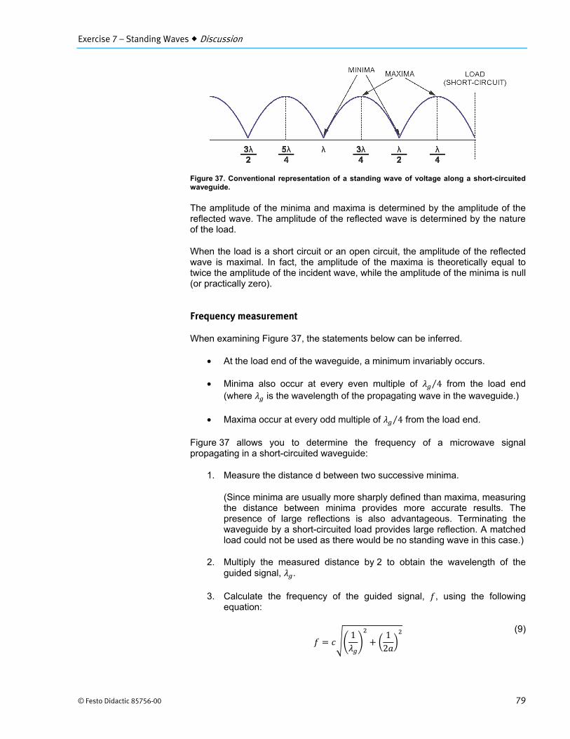
Figure 37 shows the conventional representation of a standing wave of voltage along a short-circuited waveguide.
• The points where the voltage is minimal are called minima, or nodes.
• The points where the voltage is maximal are called maxima, or loops.
Exercise 7 – Standing Waves Discussion
© Festo Didactic 85756-00 79
Figure 37. Conventional representation of a standing wave of voltage along a short-circuited waveguide.
The amplitude of the minima and maxima is determined by the amplitude of the reflected wave. The amplitude of the reflected wave is determined by the nature of the load.
When the load is a short circuit or an open circuit, the amplitude of the reflected wave is maximal. In fact, the amplitude of the maxima is theoretically equal to twice the amplitude of the incident wave, while the amplitude of the minima is null (or practically zero).
Frequency measurement
When examining Figure 37, the statements below can be inferred.
• At the load end of the waveguide, a minimum invariably occurs.
• Minima also occur at every even multiple of 4⁄ from the load end (where is the wavelength of the propagating wave in the waveguide.)
• Maxima occur at every odd multiple of 4⁄ from the load end.
Figure 37 allows you to determine the frequency of a microwave signal propagating in a short-circuited waveguide:
1. Measure the distance d between two successive minima.
(Since minima are usually more sharply defined than maxima, measuring the distance between minima provides more accurate results. The presence of large reflections is also advantageous. Terminating the waveguide by a short-circuited load provides large reflection. A matched load could not be used as there would be no standing wave in this case.)
2. Multiply the measured distance by 2 to obtain the wavelength of the guided signal, .
3. Calculate the frequency of the guided signal, , using the following equation:
= 1 + 12
(9)
Exercise 7 – Standing Waves Discussion
80 © Festo Didactic 85756-00
where is the frequency of the guided signal (Hz). is the velocity of propagation of the signal in free space
(3.0 ⋅ 108 m/s). is the wavelength of the guided signal (m). is the width of the waveguide (m).
The Slotted Line
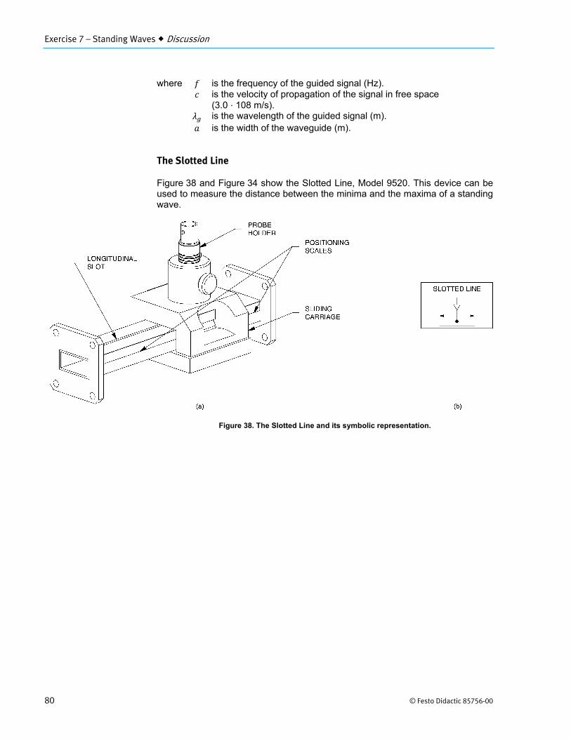
Figure 38 and Figure 34 show the Slotted Line, Model 9520. This device can be used to measure the distance between the minima and the maxima of a standing wave.
Figure 38. The Slotted Line and its symbolic representation.
Exercise 7 – Standing Waves Discussion
© Festo Didactic 85756-00 81
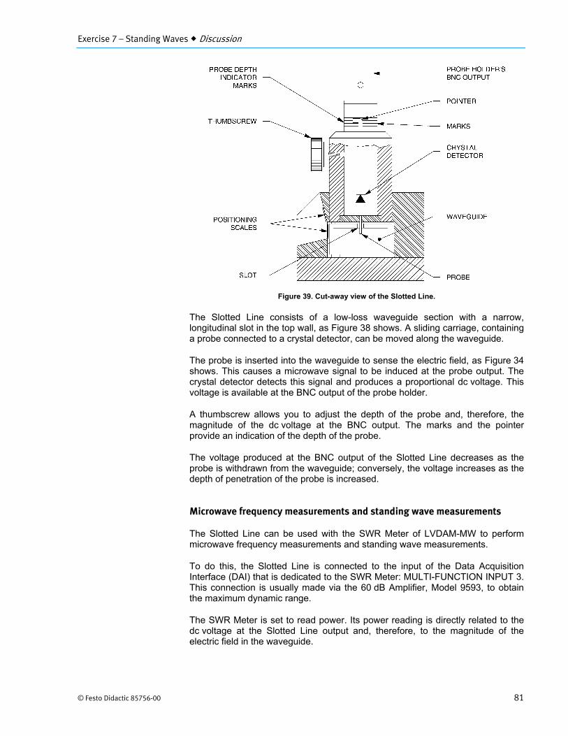
Figure 39. Cut-away view of the Slotted Line.
The Slotted Line consists of a low-loss waveguide section with a narrow, longitudinal slot in the top wall, as Figure 38 shows. A sliding carriage, containing a probe connected to a crystal detector, can be moved along the waveguide.
The probe is inserted into the waveguide to sense the electric field, as Figure 34 shows. This causes a microwave signal to be induced at the probe output. The crystal detector detects this signal and produces a proportional dc voltage. This voltage is available at the BNC output of the probe holder.
A thumbscrew allows you to adjust the depth of the probe and, therefore, the magnitude of the dc voltage at the BNC output. The marks and the pointer provide an indication of the depth of the probe.
The voltage produced at the BNC output of the Slotted Line decreases as the probe is withdrawn from the waveguide; conversely, the voltage increases as the depth of penetration of the probe is increased.
Microwave frequency measurements and standing wave measurements
The Slotted Line can be used with the SWR Meter of LVDAM-MW to perform microwave frequency measurements and standing wave measurements.
To do this, the Slotted Line is connected to the input of the Data Acquisition Interface (DAI) that is dedicated to the SWR Meter: MULTI-FUNCTION INPUT 3. This connection is usually made via the 60 dB Amplifier, Model 9593, to obtain the maximum dynamic range.
The SWR Meter is set to read power. Its power reading is directly related to the dc voltage at the Slotted Line output and, therefore, to the magnitude of the electric field in the waveguide.
Exercise 7 – Standing Waves Discussion
82 © Festo Didactic 85756-00
When the carriage is moved along the waveguide, the position of the probe changes, causing the dc voltage produced by the crystal detector to change as a function of the variation in magnitude of the electric field along the waveguide.
Two positioning scales on the waveguide and the carriage indicate the location of the carriage. This allows you to locate the minima and the maxima in the standing wave produced by various loads, and to measure the wavelength and the frequency of the microwave signal in the waveguide.
The measurements made with a slotted line are limited by the scale graduations. The accuracy of measurement decreases as the frequency of the guided signal is increased.
Start-up procedure when using the Slotted Line and the SWR Meter of LVDAM-MW
Before using the Slotted Line and the SWR Meter, the following start up procedure must be performed. This procedure allows you to obtain the maximum dynamic range on the SWR Meter, while operating the crystal detector of the Slotted Line in its square-law region to obtain valid SWR Meter readings.
1. The microwave signal injected into circuit is amplitude modulated by a 1 kHz square wave, provided by the Gunn Oscillator Power Supply. The microwave signal is then attenuated in order for the crystal detector of the Slotted Line to operate in its square-law region and the SWR Meter to provide valid readings.
2. The Slotted Line's probe is located close to the maximum nearest the load in order for the Slotted Line output voltage to be maximal. This voltage is applied to MULTI-FUNCTION INPUT 3 of the DAI (input dedicated to the SWR Meter of LVDAM-MW).
3. The depth of the Slotted Line's probe is set to the initial default position of 1/3 of maximum.
4. With the minimum sensitivity (0 dB gain) on Input 3, the frequency of the SWR Meter's amplifier is tuned to obtain the maximum signal level on the SWR Meter.
5. The Slotted Line's probe depth is then adjusted so that the maximum signal level indicated by the SWR Meter is between 70 and 90% of full scale.
6. The Slotted Line's probe is accurately positioned over the maximum, and the probe depth is fine-tuned, if necessary, to obtain the maximum signal level on the SWR Meter.
7. The reference level (0.0 dB) is set on the SWR Meter.
Particular attention must be paid to the adjustment of the probe depth inside the Slotted Line. If the probe penetrates too deep into the Slotted Line, the field distribution can be distorted, especially when the SWR is high. Moreover, the probe's crystal detector is then more likely to operate outside of its square-law region, causing the measurements to be erroneous.
Exercise 7 – Standing Waves Procedure Outline
© Festo Didactic 85756-00 83
To obtain a good accuracy of measurement, the central frequency of the SWR Meter must be readjusted whenever the microwave circuit is modified or used for a prolonged period of time, as the central frequency drifts over time. The drift in the central frequency of the SWR Meter is due, among other things, to variations in ambient temperature and equipment temperature.
Similarly, the SWR Meter's reference may vary slightly over time. Small drifts are acceptable. However, it is recommended that you verify the reference from time to time and readjust it to 0.0 dB, to maintain a good accuracy of measurement.
The Procedure is divided into the following sections:
System setup Preliminary adjustment of the Slotted Line and SWR Meter.
Measuring the guided wavelength and the microwave signal frequency Standing wave produced along the Slotted Line when the waveguide is short-circuited.
Standing wave produced along the Slotted Line when the load consists of a 6 dB attenuator and a short circuit
Standing wave produced along the Slotted Line with a matched load
System setup
In this exercise, you will measure the guided wavelength and the frequency of a microwave signal, using the Slotted Line and the SWR Meter.
You will then plot the standing-wave patterns for a short circuit, an attenuator and short-circuit load, and a matched load.
a For detailed information on how to use the SWR Meter of LVDAM-MW to perform SWR measurements, please refer to Section 3 of the User Guide "Microwave Data Acquisition and Management", part number 85756-E.
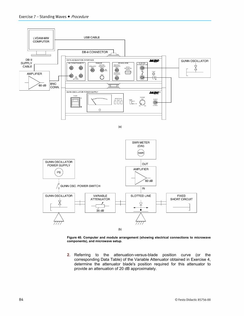
1. Make sure that all power switches are in the O (off) position. Set up the modules and assemble the microwave components as shown in Figure 40.
The Slotted Line must be connected, via the 60 dB Amplifier, to the analog input of the Data Acquisition Interface (DAI) that is dedicated to the SWR Meter of LVDAM-MW: MULTI-FUNCTION INPUT 3.
The supply cable of the 60 dB Amplifier must be connected to the DB-9 female connector on the top of the Data Acquisition Interface.
PROCEDURE OUTLINE
PROCEDURE
Exercise 7 – Standing Waves Procedure
84 © Festo Didactic 85756-00
Figure 40. Computer and module arrangement (showing electrical connections to microwave components), and microwave setup.
2. Referring to the attenuation-versus-blade position curve (or the corresponding Data Table) of the Variable Attenuator obtained in Exercise 4, determine the attenuator blade's position required for this attenuator to provide an attenuation of 20 dB approximately.
Exercise 7 – Standing Waves Procedure
© Festo Didactic 85756-00 85
Set the Variable Attenuator’s blade to this position, which will limit the microwave signal incident to the Slotted Line's crystal detector to make it operate in its square-law region.
Attenuator blade’s position = mm
3. Make the following settings on the Gunn Oscillator Power Supply:
VOLTAGE ..................................................... MIN. MODE ............................................................ 1 kHz METER SCALE ............................................. 10 V
4. Turn on the Gunn Oscillator Power Supply and the Data Acquisition Interface (DAI) by setting their POWER switch to the "I" (ON) position.
Set the Gunn Oscillator supply voltage to 8.5 V. Wait for about 5 minutes to allow the modules to warm up.
Preliminary adjustment of the Slotted Line and SWR Meter
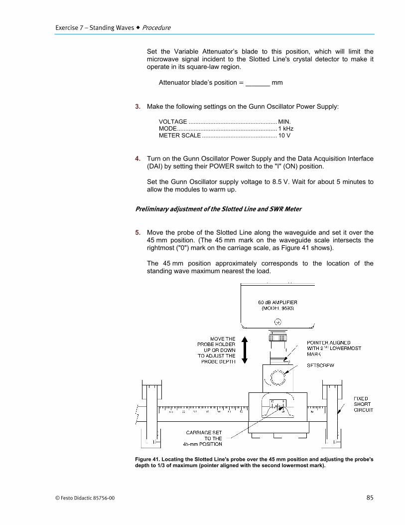
5. Move the probe of the Slotted Line along the waveguide and set it over the 45 mm position. (The 45 mm mark on the waveguide scale intersects the rightmost ("0") mark on the carriage scale, as Figure 41 shows).
The 45 mm position approximately corresponds to the location of the standing wave maximum nearest the load.
Figure 41. Locating the Slotted Line's probe over the 45 mm position and adjusting the probe's depth to 1/3 of maximum (pointer aligned with the second lowermost mark).
Exercise 7 – Standing Waves Procedure
86 © Festo Didactic 85756-00
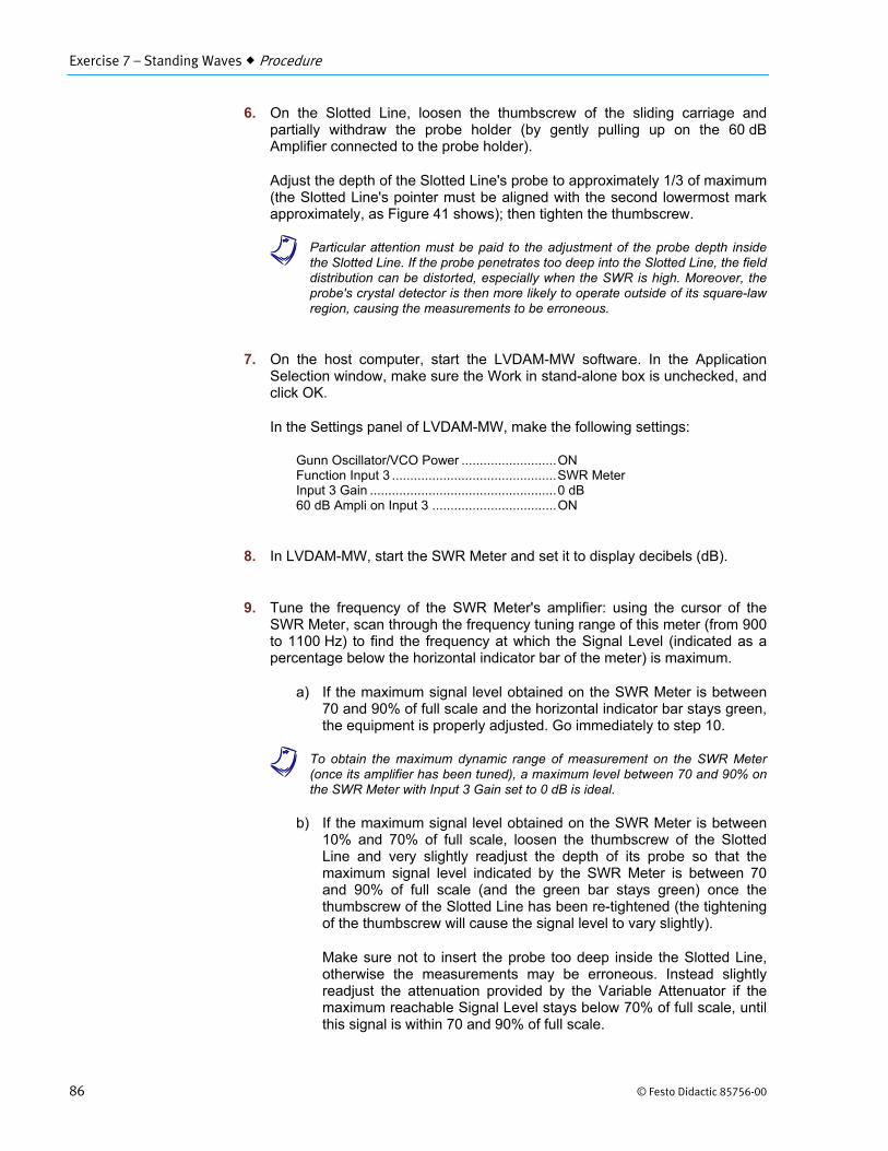
6. On the Slotted Line, loosen the thumbscrew of the sliding carriage and partially withdraw the probe holder (by gently pulling up on the 60 dB Amplifier connected to the probe holder).
Adjust the depth of the Slotted Line's probe to approximately 1/3 of maximum (the Slotted Line's pointer must be aligned with the second lowermost mark approximately, as Figure 41 shows); then tighten the thumbscrew.
a Particular attention must be paid to the adjustment of the probe depth inside the Slotted Line. If the probe penetrates too deep into the Slotted Line, the field distribution can be distorted, especially when the SWR is high. Moreover, the probe's crystal detector is then more likely to operate outside of its square-law region, causing the measurements to be erroneous.
7. On the host computer, start the LVDAM-MW software. In the Application Selection window, make sure the Work in stand-alone box is unchecked, and click OK.
In the Settings panel of LVDAM-MW, make the following settings:
Gunn Oscillator/VCO Power .......................... ON Function Input 3 ............................................. SWR Meter Input 3 Gain ................................................... 0 dB 60 dB Ampli on Input 3 .................................. ON
8. In LVDAM-MW, start the SWR Meter and set it to display decibels (dB).
9. Tune the frequency of the SWR Meter's amplifier: using the cursor of the SWR Meter, scan through the frequency tuning range of this meter (from 900 to 1100 Hz) to find the frequency at which the Signal Level (indicated as a percentage below the horizontal indicator bar of the meter) is maximum.
a) If the maximum signal level obtained on the SWR Meter is between 70 and 90% of full scale and the horizontal indicator bar stays green, the equipment is properly adjusted. Go immediately to step 10.
a To obtain the maximum dynamic range of measurement on the SWR Meter (once its amplifier has been tuned), a maximum level between 70 and 90% on the SWR Meter with Input 3 Gain set to 0 dB is ideal.
b) If the maximum signal level obtained on the SWR Meter is between 10% and 70% of full scale, loosen the thumbscrew of the Slotted Line and very slightly readjust the depth of its probe so that the maximum signal level indicated by the SWR Meter is between 70 and 90% of full scale (and the green bar stays green) once the thumbscrew of the Slotted Line has been re-tightened (the tightening of the thumbscrew will cause the signal level to vary slightly).
Make sure not to insert the probe too deep inside the Slotted Line, otherwise the measurements may be erroneous. Instead slightly readjust the attenuation provided by the Variable Attenuator if the maximum reachable Signal Level stays below 70% of full scale, until this signal is within 70 and 90% of full scale.
Exercise 7 – Standing Waves Procedure
© Festo Didactic 85756-00 87
a The adjustment process may be tedious at first, since a small change in probe depth results in a significant change in the SWR Meter's signal level, however it will become easier with practice.
c) If you are unable to tune the SWR Meter's amplifier because the maximum signal level exceeds the measurement scale (the horizontal indicator bar of the meter turns to red), loosen the thumbscrew of the Slotted Line. Readjust the depth of the Slotted Line's probe in order to obtain a significant reading on the SWR Meter (a signal level of, for example, about 25% of full scale, once the thumbscrew of the Slotted Line has been re-tightened since its tightening will cause the signal level to change slightly). Then, tune the frequency of the SWR Meter to obtain the maximum signal level on this meter. If this level is not between 70 and 90% of full scale, very slightly readjust the depth of the Slotted Line's probe so that the maximum signal level indicated by the SWR Meter is between 70 and 90% of full scale (and the green bar never turns from green to red) once the thumbscrew of the Slotted Line has been re-tightened.
d) If the maximum signal level stays null or too low (below 10% of full scale with a blue indicator bar or no bar displayed) when trying to tune the SWR Meter's amplifier, slightly decrease the attenuation produced by the Variable Attenuator in order to obtain a significant level on the SWR Meter (a signal level of, for example, about 25% of full scale). Then, tune the meter frequency in order to obtain the maximum signal level on this meter. If the maximum signal level is not between 70 and 90% of full scale, slightly readjust the Variable Attenuator for the signal to be within this range.
a The voltage produced by the Slotted Line decreases as the probe is withdrawn from the waveguide; conversely, the voltage increases as the depth of penetration of the probe is increased. The probe needs to be partially withdrawn from the Slotted Line's waveguide to obtain valid measurements on the SWR Meter and a good dynamic range. The probe must not be fully inserted into the Slotted Line's waveguide, otherwise its crystal detector may not operate in the square-law region, causing the SWR Meter readings to be erroneous.
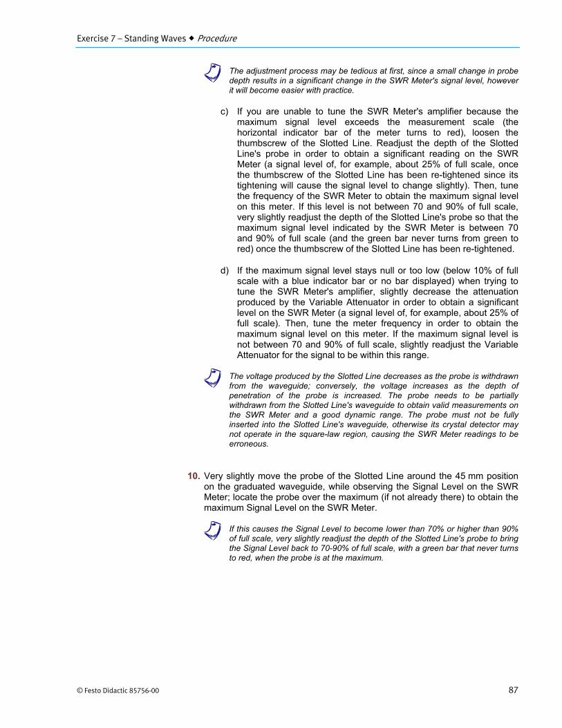
10. Very slightly move the probe of the Slotted Line around the 45 mm position on the graduated waveguide, while observing the Signal Level on the SWR Meter; locate the probe over the maximum (if not already there) to obtain the maximum Signal Level on the SWR Meter.
a If this causes the Signal Level to become lower than 70% or higher than 90% of full scale, very slightly readjust the depth of the Slotted Line's probe to bring the Signal Level back to 70-90% of full scale, with a green bar that never turns to red, when the probe is at the maximum.
Exercise 7 – Standing Waves Procedure
88 © Festo Didactic 85756-00
11. Click on the REFERENCE button of the SWR Meter to set the reference level to 0.0 dB.
Measuring the guided wavelength and the microwave signal frequency
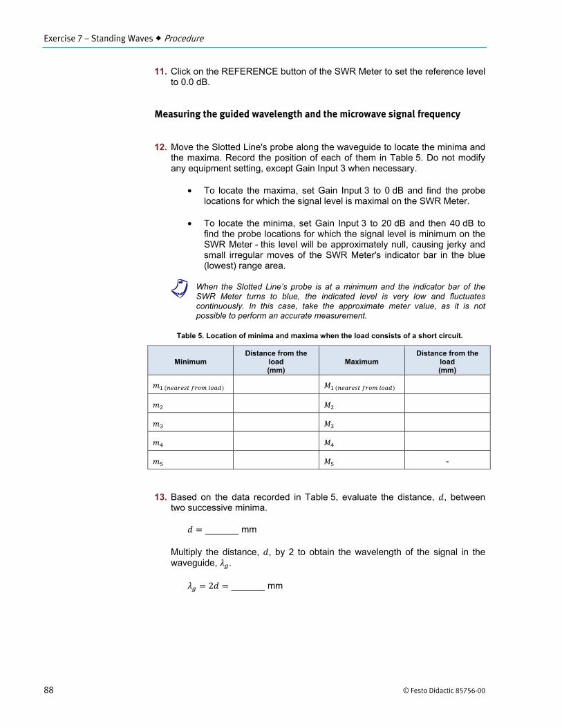
12. Move the Slotted Line's probe along the waveguide to locate the minima and the maxima. Record the position of each of them in Table 5. Do not modify any equipment setting, except Gain Input 3 when necessary.
• To locate the maxima, set Gain Input 3 to 0 dB and find the probe locations for which the signal level is maximal on the SWR Meter.
• To locate the minima, set Gain Input 3 to 20 dB and then 40 dB to find the probe locations for which the signal level is minimum on the SWR Meter - this level will be approximately null, causing jerky and small irregular moves of the SWR Meter's indicator bar in the blue (lowest) range area.
a When the Slotted Line’s probe is at a minimum and the indicator bar of the SWR Meter turns to blue, the indicated level is very low and fluctuates continuously. In this case, take the approximate meter value, as it is not possible to perform an accurate measurement.
Table 5. Location of minima and maxima when the load consists of a short circuit.
Minimum Distance from the
load (mm)
Maximum Distance from the
load (mm)
( ) ( )
-
13. Based on the data recorded in Table 5, evaluate the distance, , between two successive minima. = mm
Multiply the distance, , by 2 to obtain the wavelength of the signal in the waveguide, . = 2 = mm
Exercise 7 – Standing Waves Procedure
© Festo Didactic 85756-00 89
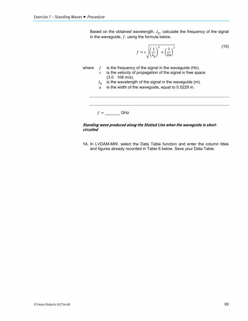
Based on the obtained wavelength, , calculate the frequency of the signal in the waveguide, , using the formula below.
= 1 + 12
(10)
where is the frequency of the signal in the waveguide (Hz). is the velocity of propagation of the signal in free space
(3.0 ⋅ 108 m/s). is the wavelength of the signal in the waveguide (m). is the width of the waveguide, equal to 0.0229 m.
= GHz
Standing wave produced along the Slotted Line when the waveguide is short-circuited
14. In LVDAM-MW, select the Data Table function and enter the column titles and figures already recorded in Table 6 below. Save your Data Table.

Exercise 7 – Standing Waves Procedure
90 © Festo Didactic 85756-00
Table 6. .⁄ ratios along the Slotted Line when the waveguide is short-circuited.
Distance from the load (mm)
SWR Meter reading (dB) .⁄
45 0 1
46
47
48
49
50
51
52
53
54
55
56
57
58
59
60
61
62
63
64
65
66
67
68
69
70
71
72
73
15. Set the Gain on Input 3 to 0 dB.
Locate the Slotted Line's probe over the maximum nearest the load (around the 45.0 mm position) in order to obtain the maximum signal level on the SWR Meter.
Verify that the frequency of the SWR Meter is properly tuned for the Signal Level displayed on the SWR Meter to be maximal. Click on the REFERENCE button of the SWR Meter to set the reference level to 0.0 dB.
Exercise 7 – Standing Waves Procedure
© Festo Didactic 85756-00 91
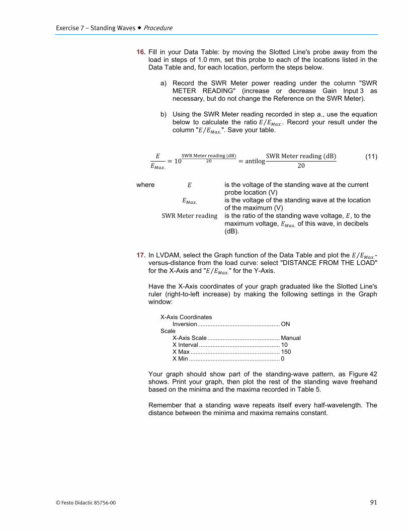
16. Fill in your Data Table: by moving the Slotted Line's probe away from the load in steps of 1.0 mm, set this probe to each of the locations listed in the Data Table and, for each location, perform the steps below.
a) Record the SWR Meter power reading under the column "SWR METER READING" (increase or decrease Gain Input 3 as necessary, but do not change the Reference on the SWR Meter).
b) Using the SWR Meter reading recorded in step a., use the equation below to calculate the ratio .⁄ . Record your result under the column " .⁄ ". Save your table.
. = 10 ( ) = antilog SWR Meter reading (dB)20 (11)
where is the voltage of the standing wave at the current
probe location (V) . is the voltage of the standing wave at the location
of the maximum (V) SWR Meter reading is the ratio of the standing wave voltage, , to the
maximum voltage, . of this wave, in decibels (dB).
17. In LVDAM, select the Graph function of the Data Table and plot the .⁄ -versus-distance from the load curve: select "DISTANCE FROM THE LOAD" for the X-Axis and " .⁄ " for the Y-Axis.
Have the X-Axis coordinates of your graph graduated like the Slotted Line's ruler (right-to-left increase) by making the following settings in the Graph window:
X-Axis Coordinates Inversion ................................................. ON
Scale X-Axis Scale ........................................... Manual X Interval ................................................ 10 X Max ..................................................... 150 X Min ...................................................... 0
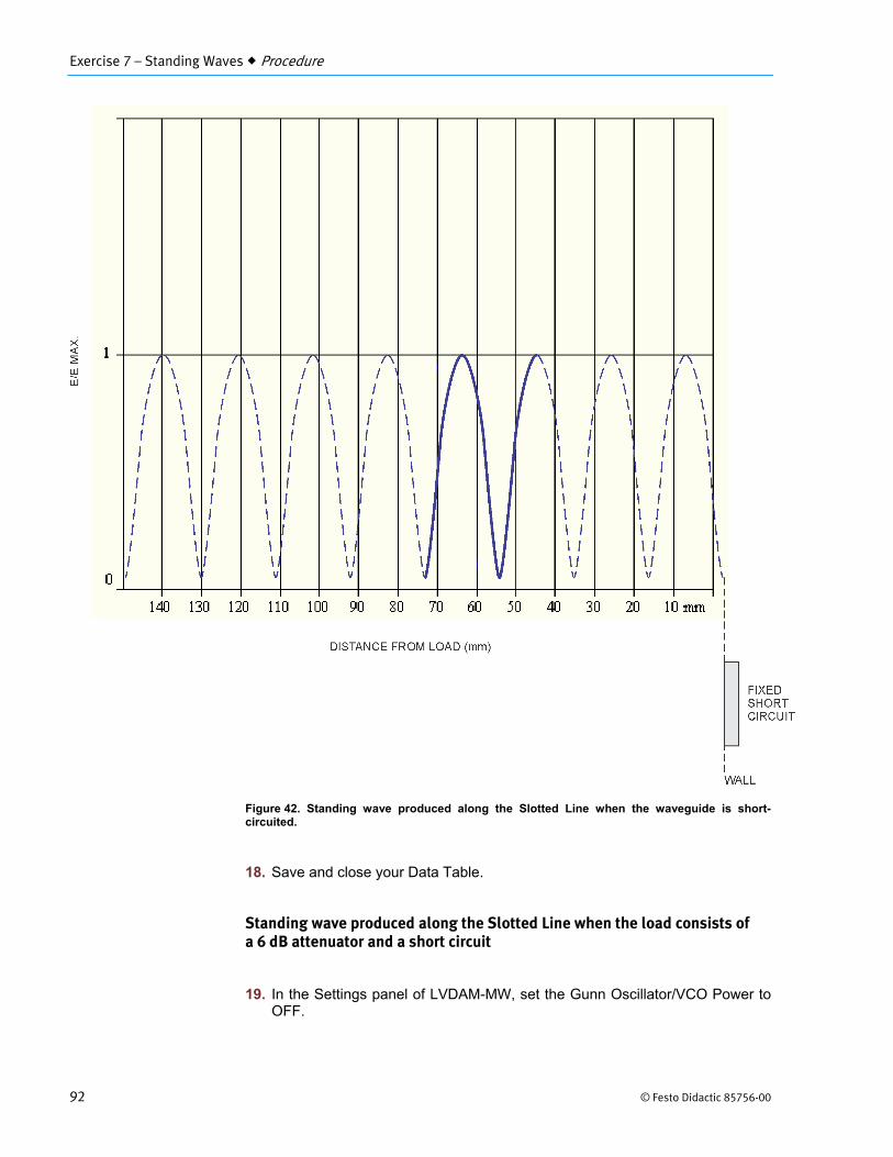
Your graph should show part of the standing-wave pattern, as Figure 42 shows. Print your graph, then plot the rest of the standing wave freehand based on the minima and the maxima recorded in Table 5.
Remember that a standing wave repeats itself every half-wavelength. The distance between the minima and maxima remains constant.
Exercise 7 – Standing Waves Procedure
92 © Festo Didactic 85756-00
Figure 42. Standing wave produced along the Slotted Line when the waveguide is short-circuited.
18. Save and close your Data Table.
Standing wave produced along the Slotted Line when the load consists of a 6 dB attenuator and a short circuit
19. In the Settings panel of LVDAM-MW, set the Gunn Oscillator/VCO Power to OFF.
Exercise 7 – Standing Waves Procedure
© Festo Didactic 85756-00 93
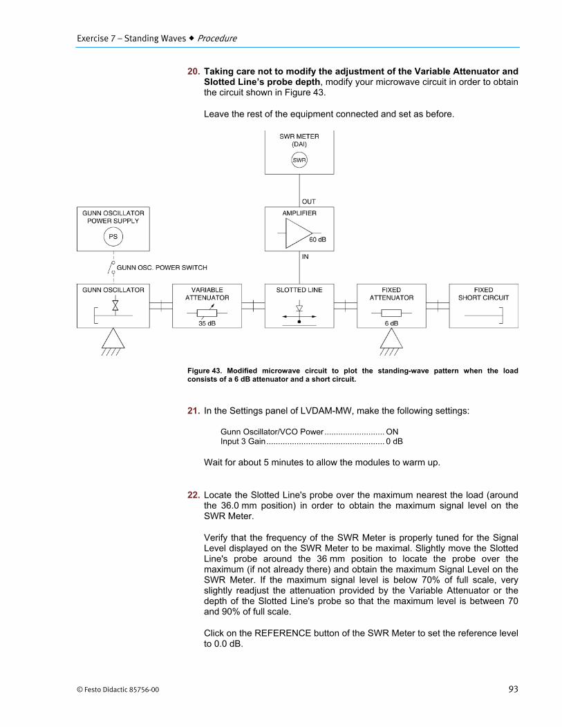
20. Taking care not to modify the adjustment of the Variable Attenuator and Slotted Line’s probe depth, modify your microwave circuit in order to obtain the circuit shown in Figure 43.
Leave the rest of the equipment connected and set as before.
Figure 43. Modified microwave circuit to plot the standing-wave pattern when the load consists of a 6 dB attenuator and a short circuit.
21. In the Settings panel of LVDAM-MW, make the following settings:
Gunn Oscillator/VCO Power .......................... ON Input 3 Gain ................................................... 0 dB
Wait for about 5 minutes to allow the modules to warm up.
22. Locate the Slotted Line's probe over the maximum nearest the load (around the 36.0 mm position) in order to obtain the maximum signal level on the SWR Meter.
Verify that the frequency of the SWR Meter is properly tuned for the Signal Level displayed on the SWR Meter to be maximal. Slightly move the Slotted Line's probe around the 36 mm position to locate the probe over the maximum (if not already there) and obtain the maximum Signal Level on the SWR Meter. If the maximum signal level is below 70% of full scale, very slightly readjust the attenuation provided by the Variable Attenuator or the depth of the Slotted Line's probe so that the maximum level is between 70 and 90% of full scale.
Click on the REFERENCE button of the SWR Meter to set the reference level to 0.0 dB.
Exercise 7 – Standing Waves Procedure
94 © Festo Didactic 85756-00
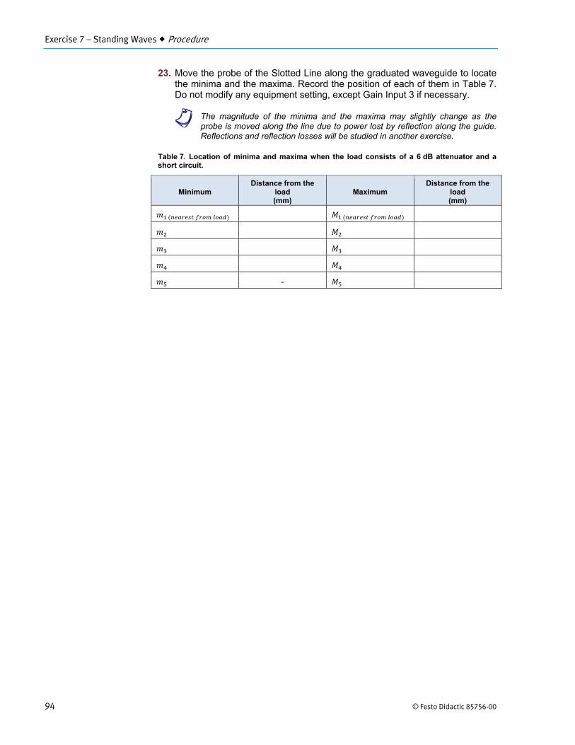
23. Move the probe of the Slotted Line along the graduated waveguide to locate the minima and the maxima. Record the position of each of them in Table 7. Do not modify any equipment setting, except Gain Input 3 if necessary.
a The magnitude of the minima and the maxima may slightly change as the probe is moved along the line due to power lost by reflection along the guide. Reflections and reflection losses will be studied in another exercise.
Table 7. Location of minima and maxima when the load consists of a 6 dB attenuator and a short circuit.
Minimum Distance from the
load (mm)
Maximum Distance from the
load (mm) ( ) ( )
-

Exercise 7 – Standing Waves Procedure
© Festo Didactic 85756-00 95
24. In LVDAM-MW, select the Data Table function and enter the column titles and figures already recorded in Table 8 below. Save your Data Table.
Table 8. .⁄ ratios along the Slotted Line when the load consists of a 6 dB attenuator and a short circuit.
Distance from the load (mm)
SWR Meter reading (dB) .⁄
36 0 1
37
38
39
40
41
42
43
44
45
46
47
48
49
50
51
52
53
54
55
56
57
58
59
60
61
62
63
64
25. Locate the Slotted Line's probe over the maximum nearest the load (around the 36.0 mm position) in order to obtain the maximum signal level on the SWR Meter.
Verify that the frequency of the SWR Meter is properly tuned for the Signal Level displayed on the SWR Meter to be maximal. Click on the REFERENCE button of the SWR Meter to set the reference level to 0.0 dB.
Exercise 7 – Standing Waves Procedure
96 © Festo Didactic 85756-00
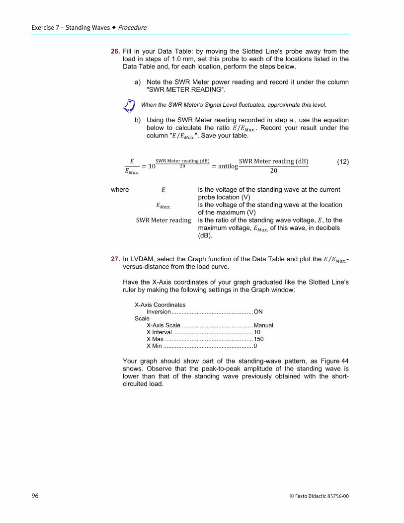
26. Fill in your Data Table: by moving the Slotted Line's probe away from the load in steps of 1.0 mm, set this probe to each of the locations listed in the Data Table and, for each location, perform the steps below.
a) Note the SWR Meter power reading and record it under the column "SWR METER READING".
a When the SWR Meter's Signal Level fluctuates, approximate this level.
b) Using the SWR Meter reading recorded in step a., use the equation below to calculate the ratio .⁄ . Record your result under the column " .⁄ ". Save your table.
. = 10 ( ) = antilog SWR Meter reading (dB)20 (12)
where is the voltage of the standing wave at the current
probe location (V) . is the voltage of the standing wave at the location
of the maximum (V) SWR Meter reading is the ratio of the standing wave voltage, , to the
maximum voltage, . of this wave, in decibels (dB).
27. In LVDAM, select the Graph function of the Data Table and plot the .⁄ -versus-distance from the load curve.
Have the X-Axis coordinates of your graph graduated like the Slotted Line's ruler by making the following settings in the Graph window:
X-Axis Coordinates Inversion ................................................. ON
Scale X-Axis Scale ........................................... Manual X Interval ................................................ 10 X Max ..................................................... 150 X Min ...................................................... 0
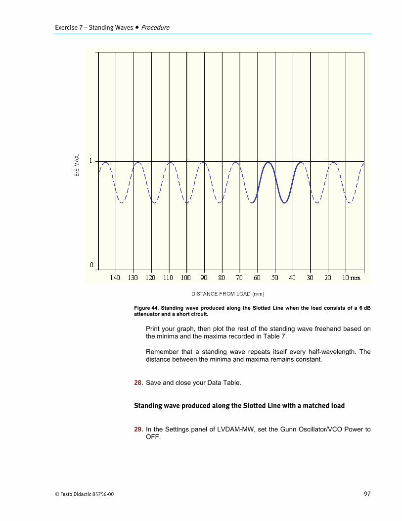
Your graph should show part of the standing-wave pattern, as Figure 44 shows. Observe that the peak-to-peak amplitude of the standing wave is lower than that of the standing wave previously obtained with the short-circuited load.
Exercise 7 – Standing Waves Procedure
© Festo Didactic 85756-00 97
Figure 44. Standing wave produced along the Slotted Line when the load consists of a 6 dB attenuator and a short circuit.
Print your graph, then plot the rest of the standing wave freehand based on the minima and the maxima recorded in Table 7.
Remember that a standing wave repeats itself every half-wavelength. The distance between the minima and maxima remains constant.
28. Save and close your Data Table.
Standing wave produced along the Slotted Line with a matched load
29. In the Settings panel of LVDAM-MW, set the Gunn Oscillator/VCO Power to OFF.
Exercise 7 – Standing Waves Procedure
98 © Festo Didactic 85756-00
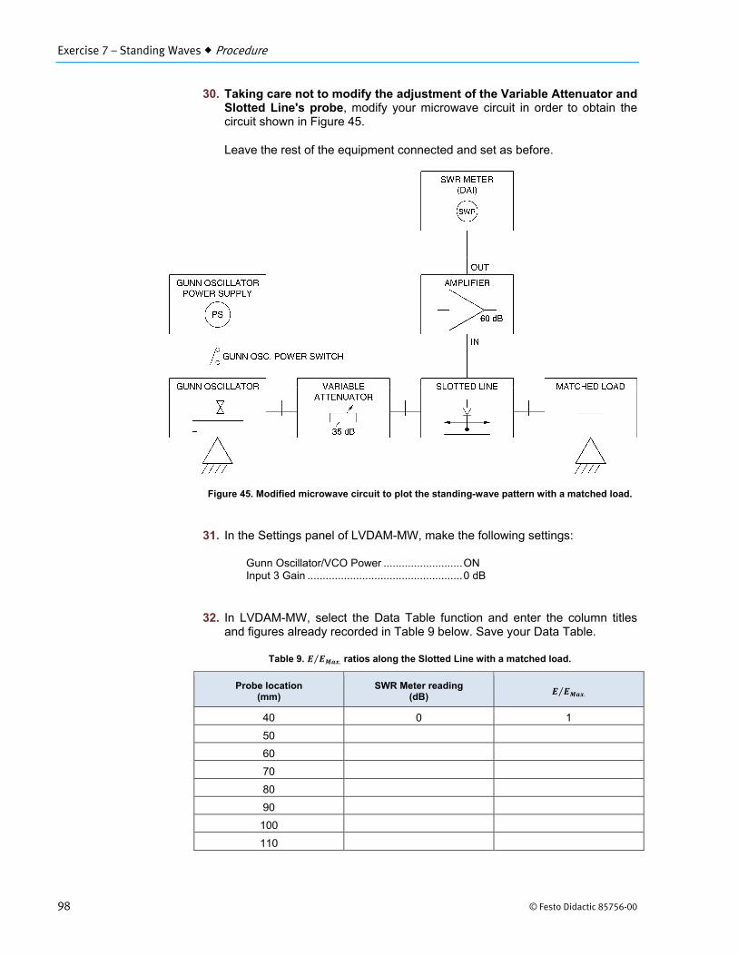
30. Taking care not to modify the adjustment of the Variable Attenuator and Slotted Line's probe, modify your microwave circuit in order to obtain the circuit shown in Figure 45.
Leave the rest of the equipment connected and set as before.
Figure 45. Modified microwave circuit to plot the standing-wave pattern with a matched load.
31. In the Settings panel of LVDAM-MW, make the following settings:
Gunn Oscillator/VCO Power .......................... ON Input 3 Gain ................................................... 0 dB
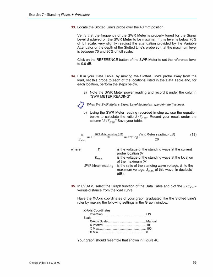
32. In LVDAM-MW, select the Data Table function and enter the column titles and figures already recorded in Table 9 below. Save your Data Table.
Table 9. .⁄ ratios along the Slotted Line with a matched load.
Probe location (mm)
SWR Meter reading (dB) .⁄
40 0 1
50
60
70
80
90
100
110
Exercise 7 – Standing Waves Procedure
© Festo Didactic 85756-00 99
33. Locate the Slotted Line's probe over the 40 mm position.
Verify that the frequency of the SWR Meter is properly tuned for the Signal Level displayed on the SWR Meter to be maximal. If this level is below 70% of full scale, very slightly readjust the attenuation provided by the Variable Attenuator or the depth of the Slotted Line's probe so that the maximum level is between 70 and 90% of full scale.
Click on the REFERENCE button of the SWR Meter to set the reference level to 0.0 dB.
34. Fill in your Data Table: by moving the Slotted Line's probe away from the load, set this probe to each of the locations listed in the Data Table and, for each location, perform the steps below.
a) Note the SWR Meter power reading and record it under the column "SWR METER READING".
a When the SWR Meter's Signal Level fluctuates, approximate this level.
b) Using the SWR Meter reading recorded in step a., use the equation below to calculate the ratio .⁄ . Record your result under the column " .⁄ " Save your table.
. = 10 ( ) = antilog SWR Meter reading (dB)20 (13)
where is the voltage of the standing wave at the current
probe location (V) . is the voltage of the standing wave at the location
of the maximum (V) SWR Meter reading is the ratio of the standing wave voltage, , to the
maximum voltage, . of this wave, in decibels (dB).
35. In LVDAM, select the Graph function of the Data Table and plot the .⁄ -versus-distance from the load curve.
Have the X-Axis coordinates of your graph graduated like the Slotted Line's ruler by making the following settings in the Graph window:
X-Axis Coordinates Inversion ................................................. ON
Scale X-Axis Scale ........................................... Manual X Interval ................................................ 10 X Max ..................................................... 150 X Min ...................................................... 0
Your graph should resemble that shown in Figure 46.
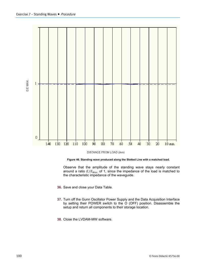
Exercise 7 – Standing Waves Procedure
100 © Festo Didactic 85756-00
Figure 46. Standing wave produced along the Slotted Line with a matched load.
Observe that the amplitude of the standing wave stays nearly constant around a ratio .⁄ of 1, since the impedance of the load is matched to the characteristic impedance of the waveguide.
36. Save and close your Data Table.
37. Turn off the Gunn Oscillator Power Supply and the Data Acquisition Interface by setting their POWER switch to the O (OFF) position. Disassemble the setup and return all components to their storage location.
38. Close the LVDAM-MW software.

Exercise 7 – Standing Waves Conclusion
© Festo Didactic 85756-00 101
In this exercise, the concepts of characteristic impedance, reflected waves, and standing-waves were introduced. You became familiar with the use of a slotted line by evaluating the guided wavelength and the frequency of a microwave signal. You also determined the standing-wave patterns for a short circuit, an attenuator and short-circuit load, and a matched load.
1. What does a standing-wave pattern represent?
2. What is the distance, in terms of wavelengths, between successive minima in a standing-wave pattern?
3. What causes a maximum on a standing-wave?
4. Explain how to determine a microwave signal's frequency with a slotted line.
5. What physical parameter does a slotted line measure?
CONCLUSION
REVIEW QUESTIONS


Sample
Extracted from
Instructor Guide

© Festo Didactic 85756-10 23
The Discussion of this exercise covers the following points:
Introductory information Microwave frequency measurements and standing wave plotting with the
Slotted Line and LVDAM-MW SWR Meter Startup procedure when using the Slotted Line and the SWR Meter of LVDAM-MW.
Instructional plan Demonstrations Presentation aids
Introductory information
Exercise 7 introduces standing waves. Standing waves are the result of two waves of the same frequency and amplitude travelling in opposite directions in a waveguide adding to and subtracting from each other. In waveguides, two waves travelling in opposite directions exist when an incident wave encounters a discontinuity, obstacle, or load and a reflected wave is produced. A standing wave can be defined for any component of the microwave field. Generally, the electric field component is considered.
When the two waves are of the same magnitude, the resulting wave is called a pure standing wave. This wave is stationary; that is, a constant-phase point does not move, but remains at the same point as time goes by. If one of the waves is smaller than the other, the resulting wave will not be stationary and the constant-phase point will move in the same direction as the larger wave. However, the envelope of the instantaneous curves will be stationary. This envelope is called a standing-wave pattern.
Normally, it is not the shape of the standing-wave pattern that is of interest; it is rather the ratio of the maximum to the minimum values of the pattern, called the standing-wave ratio (SWR), that is of interest. A maximum of a standing-wave pattern is the sum of the amplitudes of the two waves. A minimum is the difference between the amplitudes of the two waves.
A common cause of standing-wave patterns is the reflection of a portion of the propagating wave by a load in the microwave system. If the impedance of the load is not equal to the characteristic impedance of the system, some of the propagating wave will be reflected back towards the microwave source. The size of the reflected wave will depend on the mismatch between the load and the system. Obviously, if a part of the signal sent to the load is reflected, the load will not have absorbed all of the signal. From the SWR produced by the resulting standing-wave pattern, you can determine the fraction of the incident wave that has been reflected.
Standing Waves
Exercise 7
DISCUSSION OUTLINE
DISCUSSION
Exercise 7 – Standing Waves Discussion
24 © Festo Didactic 85756-10
In the first part of the exercise, the students will use the Slotted Line and the SWR Meter of LVDAM-MW to measure the guided wavelength of a microwave signal. To do this, the students will first measure the distance between two successive minima near the load (in the short-circuited condition) and multiply this distance by two to obtain the wavelength. Based on this wavelength, the students will use a formula to calculate the frequency of the microwave signal.
The students will then use the Slotted Line and the SWR Meter to determine the standing-wave pattern produced by three different loads: a short circuit, an attenuator and short-circuit load, and a matched load. The students will record and save all the measurements made with the Slotted Line and the SWR Meter in the Data Table of LVDAM-MW; the Graph function of this software will automatically plot the standing-wave pattern corresponding to the results recorded in the Data Table.
Microwave frequency measurements and standing wave plotting with the Slotted Line and LVDAM-MW SWR Meter
The Slotted Line is used with the SWR Meter of LVDAM-MW to perform microwave frequency measurements and standing wave plotting.
To do this, the Slotted Line must be connected to the input of the Data Acquisition Interface (DAI) that is dedicated to the SWR Meter: MULTI-FUNCTION INPUT 3. This connection is usually made via the 60 dB Amplifier, Model 9593, to obtain the maximum dynamic range.
The SWR Meter is set to read power, in dB. Its power reading is directly related to the dc voltage at the Slotted Line output and, therefore, to the magnitude of the electric field in the waveguide.
When the carriage is moved along the waveguide, the position of the probe changes, causing the dc voltage produced by the Slotted Line’s crystal detector to change as a function of the variation in magnitude of the electric field along the waveguide.
Two positioning scales on the waveguide and the carriage indicate the location of the carriage. This allows the students to locate the minima and the maxima in the standing wave produced by various loads, and to measure the wavelength and the frequency of the microwave signal in the waveguide.
The measurements made with the Slotted Line are limited by the scale graduations.
Startup procedure when using the Slotted Line and the SWR Meter of LVDAM-MW
a For detailed information on this startup procedure, please refer to Section 3 of the User Guide Microwave Data Acquisition and Management, part number 85756-E.
Before using the Slotted Line and the SWR Meter, the following startup procedure must be performed. This procedure allows students to obtain the maximum dynamic range on the SWR Meter, while operating the crystal detector of the Slotted Line in its square-law region to obtain valid SWR Meter readings.
Exercise 7 – Standing Waves Discussion
© Festo Didactic 85756-10 25
1. The microwave signal injected into the circuit is amplitude modulated by a 1 kHz square wave, provided by the Gunn Oscillator Power Supply. The microwave signal is then attenuated in order for the crystal detector of the Slotted Line to operate in its square-law region and the SWR Meter to provide valid readings.
2. The Slotted Line's probe is located over the standing-wave maximum nearest the load in order for the Slotted Line output voltage to be maximum. This voltage is applied to MULTI-FUNCTION INPUT 3 (input dedicated to the SWR Meter of LVDAM-MW).
3. The depth of the Slotted Line's probe is set to the initial default position of 1/3 of maximum.
4. With the minimum sensitivity (0 dB gain) on MULTI-FUNCTION INPUT 3, the frequency of the SWR Meter's amplifier is tuned to obtain the maximum signal level on the SWR Meter.
5. The Slotted Line's probe depth is then adjusted so that the maximum signal level indicated by the SWR Meter is between 70 and 90% of full scale.
6. The Slotted Line's probe is accurately positioned over the maximum, and the probe depth is fine-tuned, if necessary, to obtain the maximum signal level on the SWR Meter.
7. Finally, the reference level (0.0 dB) is set on the SWR Meter. All subsequent SWR Meter readings will be the ratio, in decibels (dB), of the measured power to the reference level of 0.0 dB (relative power level).
Particular attention must be paid to the adjustment of the probe depth inside the Slotted Line. If the probe penetrates too deep into the Slotted Line, the field distribution can be distorted, especially when the SWR is high. Moreover, the probe's crystal detector is then more likely to operate outside of its square-law region, causing the measurements to be erroneous.
To obtain a good accuracy of measurement, the tuning of the amplifier frequency of the SWR Meter must be readjusted whenever the microwave circuit is modified or used for a prolonged period of time, as the central frequency drifts over time. The drift in the central frequency of the SWR Meter’s amplifier is due, among other things, to variations in ambient temperature and equipment temperature.
Similarly, the SWR Meter's reference may vary slightly over time. Small drifts are acceptable. However, it is recommended that you verify the reference from time to time and readjust it to 0.0 dB, to maintain a good accuracy of measurement.
Instructional plan
A. Explain how standing-wave patterns are formed from two waves travelling in opposite directions:
1. Waves of the same frequency and amplitude (produce a pure standing wave).
Exercise 7 – Standing Waves Discussion
26 © Festo Didactic 85756-10
2. Waves of the same frequency, but different amplitude (produce a standing-wave pattern).
B. Describe a standing-wave pattern showing the minima and maxima. Emphasize the fact that the distance between successive minima or maxima is equal to half the guided wavelength of the microwave signal.
C. Briefly explain that the size of the reflected wave depends on the mismatch between the characteristic impedance of the waveguide system and the impedance of the load.
D. Briefly explain the standing-wave ratio. (More will be said about the SWR in Exercise 10):
E. Familiarize the students with the Slotted Line.
F. Explain how to use the SWR Meter of LVDAM-MW to perform measurements with the Slotted Line, and the startup procedure to perform.
G. Explain how the Slotted Line and the SWR Meter are used to determine the guided wavelength of the microwave signal:
1. Measure the distance between successive minima. Also explain why minima are used rather than maxima.
2.
1 12
(4)
where is the frequency of the signal in the waveguide (Hz). is the velocity of propagation of the signal in free space (3.0 x
108 m/s) is the wavelength of the signal in the waveguide (m). is the width of the waveguide, equal to 0.0229 m.
Demonstrations
Show why minima of the standing-wave pattern are used to determine the wavelength of a signal in the guide. You could use a sketch of a standing-wave pattern and a set-up with a Slotted Line and a Fixed Short Circuit. Show that the precise location of a minimum is much easier to determine than that of a maximum.
By changing loads, show that, although the standing-wave pattern may shift and its amplitude may vary, the distance between minima and maxima remains constant.
Exercise 7 – Standing Waves Discussion
© Festo Didactic 85756-10 27
Presentation aids
1. Use diagrams to show how a standing-wave pattern is formed. Many textbooks have diagrams that might prove helpful.
2. Use the explanations given above to explain how to use the SWR Meter with the Slotted Line and how to perform the startup procedure. The User Guide (part number 85756-E) gives the detailed startup procedure.

© Festo Didactic 85756-00 419
Bibliography
BADENFULLER, A.J., Microwaves: An Introduction to Microwave Theory and Techniques, 2nd Edition, Oxford, U.K., Pergammon Press, 1979. ISBN 0-08-024297-8
CHEUNG, W.S., LEVIEW, F.H., Microwave Made Simple. Principles and Applications, Dadham, Mass (U.S.A.), Artech House Inc., 1985. ISBN 0-89006-173-4
CROSS, A.W., Experimental Microwave, Stevenage, U.K., Marconi Instruments Ltd., 1977.
GANDHI, O.P., Microwave Engineering and Applications, Elsmsford, New York, Pergamon Press Inc., 1981. ISBN 0-08-025588-4
GARDIOL, F., Hyperfréquences, Paris, France, Dunod, 1987. ISBN 2-04-016953-9
GRIVET, P., Physique des Lignes de Haute Fréquence et d'Ultra-Haute Fréquence, Paris, France, Masson et Cie, 1969.
GUPTA, K.C., Microwaves, New Delhi, India, Wiley Eastern Ltd., 1979. ISBN 0-85226-346-5
JOUQUET, M., Ondes Électromagnétiques – Vol. 2: Propagation Guidée, Paris, France, Bordas-Dunod, 1973. ISBN 2-04-010141-1
KENNEDY, G., Electric Communication Systems, 3rd Ed., New York, N.Y. (U.S.A.), McGraw Hill Book Co., 1985. ISBN 0-070-34054-4
LAVERGHETTA, T.S., Handbook of Microwave Testing, Dadham, Mass (U.S.A.), Artech House Inc., 1981. ISBN 0-89006-070-3
LIAO, S.Y., Microwave Devices and Circuits, Englewood Cliffs, New Jersey (U.S.A.), Prentice Hall Inc., 1980. ISBN 0-13-581297-0
VASSALLO, C., Théorie des Guides d'Ondes Électromagnétiques – Tome 1 et Tome 2, Paris, France, Éditions Eyrolles, 1985.

This page should be left blank


![B.E. Sem. VII [EXTC] Fundamentals of Microwave …vidyalankar.org/file/engg_degree/prelim_paper_soln/SemVII/EXTC/... · Fundamentals of Microwave Engineering Prelim Question Paper](https://img.pdfslide.us/doc/110x75/5ab168727f8b9ad9788c3916/be-sem-vii-extc-fundamentals-of-microwave-of-microwave-engineering-prelim.jpg)