Embed Size (px)
Citation preview
HAL Id: tel-00755876https://tel.archives-ouvertes.fr/tel-00755876
Submitted on 22 Nov 2012
HAL is a multi-disciplinary open accessarchive for the deposit and dissemination of sci-entific research documents, whether they are pub-lished or not. The documents may come fromteaching and research institutions in France orabroad, or from public or private research centers.
L’archive ouverte pluridisciplinaire HAL, estdestinée au dépôt et à la diffusion de documentsscientifiques de niveau recherche, publiés ou non,émanant des établissements d’enseignement et derecherche français ou étrangers, des laboratoirespublics ou privés.
Search for Higgs boson in the WW* channel in ATLASand drift time measurement in the liquid argon
calorimeter in ATLASXifeng Ruan
To cite this version:Xifeng Ruan. Search for Higgs boson in the WW* channel in ATLAS and drift time measurementin the liquid argon calorimeter in ATLAS. Other [cond-mat.other]. Université Paris Sud - Paris XI;Institute of high energy physics (Chine), 2012. English. �NNT : 2012PA112236�. �tel-00755876�
UNIVERSITE PARIS-SUD
Ecole doctorale: 517 - Particules, Noyaux et CosmosLaboratoire de l’Accelerateur Lineaire
Discipline: Physique des particules
THESE DE DOCTORAT
Presentee par Xifeng RUAN
Search for Higgs boson in theWW (∗) channel in ATLAS anddrift time measurement in the
liquid argon calorimeter in ATLASRecherche du boson de Higgs dans le canal
WW (∗) dans l’experience ATLAS et mesure dutemps de derive du calorimetre a argon liquide
dans l’experience ATLAS
Soutenue le 19 Oct 2012 devant le jury compose de:
Directeur de these: Zhiqing Zhang LALCo-directeur de these: Shan Jin IHEPPresident et Rapporteur: Yuanning Gao Tsinghua Univ.Rapporteur: Samira Hassani IRFUExaminateur: Congfeng Qiao UCASExaminateur: Guoming Chen IHEP
ResumeUne recherche du boson de Higgs est effectuee dans le canal WW → lνlν en utilisantl’ensemble des donnees de 2011 a une energie dans le centre de masse de
√s = 7 TeV
et une partie des donnees de 2012 a 8 TeV prises par l’experience ATLAS aupresdu LHC. Les luminosites integrees correspondantes sont 4.7 fb−1 et 5.8 fb−1, respec-tivement. Plusieurs methodes sont introduites pour estimer a partir des donnees lacontribution de bruits de fond des differents processus afin de minimiser l’utilisationde la simulation. Pour la contribution du bruit de fond top dans le canal domi-nant avec zero jet, elle est estimee avec une mthode que nous avons proposee. Uneautre methode pour corriger la forme de la distribution de l’energie transverse man-quante dans les evenements Drell-Yan a partir des evenements W+jets est egalementpresentee. En 2011, le boson de Higgs du modele standard avec la masse du Higgs de133 a 261 GeV est exclue a 95% de niveau de confiance, tandis que la plage d’exclusionprevue est de 127 a 234 GeV. En 2012, un exces d’evenements au-dessus du bruit defond attendu est observe dans une plage de masse autour de 125 GeV. En combinantles deux echantillons, la probabilite minimale (“p-value”) pour que l’hypothese bruitde fond seul fournisse autant ou plus d’evenements qu’observe dans les donnees est de3 × 10−3, ce qui correspond a une signifiance statistique de 2,8 ecarts types. Le tauxde production mesure du signal par rapport au taux predit pour le boson de Higgs dumodele standard a mH = 125 GeV est de 1, 4± 0, 5. La probabilite attendue pour unHiggs avec mH = 125 GeV est de 0,01, soit de 2,3 ecarts types. La limite d’exclusiond’un Higgs dans un modele avec une quatrieme generation est egalement presenteeen utilisant une partie de l’echantillon de donnees 2011, la gamme de masse entre120 GeV et 600 GeV a ete exclue a 95% de niveau de confiance. Enfin, l’etude sur letemps de derive dans le calorimetre a argon liquide du detecteur ATLAS est effectueeen utilisant tous les echantillons de donnees du rayonnement cosmique, du faisceausplash et de collision. Les resultats ne montrent aucune non-uniformite significativesur la largeur de l’espace cellulaire mis a part un effet de “sagging” dans les regionsde transition du au poids du calorimetre.
Mots-cles: Modele standard, Higgs, quatrieme generation,WW , temps de derive,calorimetre
AbstractA Higgs search is performed in the WW → lνlν channel using the full 2011 data ata center-of-mass energy of
√s = 7TeV and part of 2012 data at 8 TeV taken by the
ATLAS experiment at the LHC. The corresponding integrated luminosity values are4.7 fb−1 and 5.8 fb−1, respectively. The cut based analysis is performed and severaldata-driven methods for background estimation are introduced. The jet veto survivalprobability method for top background estimation in 0-jet bin is proposed and usedin the Higgs search. Another data-driven method to correct Emiss
T shapes in the Drell-Yan process is also presented. In 2011, the standard model Higgs boson with the Higgsmass from 133 to 261 GeV is excluded at 95%CL, while the expected exclusion rangeis 127−234 GeV. In 2012, an excess of events over expected background is observed at

mH = 125 GeV. Combining both samples, the minimum observed p0 value is 3×10⁻³,corresponding to 2.8 standard deviations. The fitted signal strength atmH = 125 GeVis µ = 1.4 ± 0.5. The expected p0 for a Higgs with mH = 125 GeV is 0.01, or 2.3standard deviations. The exclusion limit for a Higgs in a fourth generation modelis shown using part of the 2011 data sample, the mass range between 120GeV and600 GeV has been excluded at 95%CL. The study of the drift time in the liquid argoncalorimeter in ALTAS is performed using all special data samples from cosmic muons,beam splash and beam collision data. The results show no significant non-uniformityon the cell gap width and a sagging effect due to gravity is observed.
Keywords : Standard model, Higgs, fourth generation,WW , drift time, calorime-ter.
2
Contents
1 Introduction to the Standard Model and Higgs 81.1 The Standard Model . . . . . . . . . . . . . . . . . . . . . . . . . . . 81.2 Symmetry and Dynamics . . . . . . . . . . . . . . . . . . . . . . . . . 9
1.2.1 QED . . . . . . . . . . . . . . . . . . . . . . . . . . . . . . . . 101.2.2 QCD . . . . . . . . . . . . . . . . . . . . . . . . . . . . . . . . 101.2.3 GWS theory . . . . . . . . . . . . . . . . . . . . . . . . . . . . 11
1.3 Higgs Physics . . . . . . . . . . . . . . . . . . . . . . . . . . . . . . . 121.3.1 The Higgs Mechanism . . . . . . . . . . . . . . . . . . . . . . 121.3.2 Higgs Production at the LHC . . . . . . . . . . . . . . . . . . 141.3.3 Constraints on Higgs Mass . . . . . . . . . . . . . . . . . . . . 14
2 The Large Hadron Collider and ATLAS Detector 212.1 The Large Hadron Collider . . . . . . . . . . . . . . . . . . . . . . . . 212.2 ATLAS Detector . . . . . . . . . . . . . . . . . . . . . . . . . . . . . 23
2.2.1 Magnet system . . . . . . . . . . . . . . . . . . . . . . . . . . 252.2.2 Inner detector . . . . . . . . . . . . . . . . . . . . . . . . . . . 252.2.3 Calorimeter . . . . . . . . . . . . . . . . . . . . . . . . . . . . 282.2.4 Muon Spectrometer . . . . . . . . . . . . . . . . . . . . . . . . 312.2.5 The ATLAS trigger system . . . . . . . . . . . . . . . . . . . . 322.2.6 The Luminosity Detectors . . . . . . . . . . . . . . . . . . . . 33
3 Objects Reconstruction, Identification and Selection 353.1 Electrons . . . . . . . . . . . . . . . . . . . . . . . . . . . . . . . . . . 35
3.1.1 Electron Reconstruction . . . . . . . . . . . . . . . . . . . . . 353.1.2 Electron Identification and Selection in Higgs Analyses . . . . 36
3.2 Muons . . . . . . . . . . . . . . . . . . . . . . . . . . . . . . . . . . . 413.2.1 Muon Reconstruction . . . . . . . . . . . . . . . . . . . . . . . 413.2.2 Muons Selection in H → WW (∗) Analysis . . . . . . . . . . . 42
3.3 Jets . . . . . . . . . . . . . . . . . . . . . . . . . . . . . . . . . . . . 433.3.1 Jets Reconstruction and Calibration . . . . . . . . . . . . . . 433.3.2 Jets Flavour Identification and Selection . . . . . . . . . . . . 44
3.4 Transverse Missing Energy . . . . . . . . . . . . . . . . . . . . . . . . 453.5 Luminosity Determination . . . . . . . . . . . . . . . . . . . . . . . . 46
3
4 Event Selection in Higgs to WW (∗) to lνlν Analysis 484.1 Data Sample . . . . . . . . . . . . . . . . . . . . . . . . . . . . . . . . 494.2 Monte Carlo Samples and Simulations . . . . . . . . . . . . . . . . . 494.3 Trigger Requirements . . . . . . . . . . . . . . . . . . . . . . . . . . . 504.4 Event Selection . . . . . . . . . . . . . . . . . . . . . . . . . . . . . . 52
4.4.1 Common Event Selection . . . . . . . . . . . . . . . . . . . . . 524.4.2 Jet Bin Dependent Selections . . . . . . . . . . . . . . . . . . 54
4.5 Systematic Uncertainties . . . . . . . . . . . . . . . . . . . . . . . . . 64
5 Background Estimation 735.1 Introduction . . . . . . . . . . . . . . . . . . . . . . . . . . . . . . . . 735.2 W+jets Background Estimation . . . . . . . . . . . . . . . . . . . . . 745.3 Top Background Estimation . . . . . . . . . . . . . . . . . . . . . . . 75
5.3.1 Description of the Top Process . . . . . . . . . . . . . . . . . . 755.3.2 Methodology and MC Truth Study . . . . . . . . . . . . . . . 785.3.3 Data-Driven Top Estimate for 2011 Data Analysis . . . . . . . 825.3.4 Systematics Study . . . . . . . . . . . . . . . . . . . . . . . . 825.3.5 Top Background Estimation in 1- and 2-Jet Bins . . . . . . . 93
5.4 Z/Drell-Yan Background Estimation and Constraint on EmissT Mismod-
elling Using W+jets Events . . . . . . . . . . . . . . . . . . . . . . . 955.4.1 ABCD Method . . . . . . . . . . . . . . . . . . . . . . . . . . 955.4.2 Scale Factor Method . . . . . . . . . . . . . . . . . . . . . . . 975.4.3 Constraint on Emiss
T Mismodelling Using W+jets Events . . . 985.5 SM WW backgrounds . . . . . . . . . . . . . . . . . . . . . . . . . . 106
6 Results of Higgs Search in 2011 1176.1 Statistical Analysis Basis . . . . . . . . . . . . . . . . . . . . . . . . . 1176.2 Results for a Fourth generation Higgs Search . . . . . . . . . . . . . . 1196.3 Results for SM Higgs Search with 2011 Data . . . . . . . . . . . . . . 122
7 Results of Higgs Search in 2012 1277.1 Improvements and New Features in 2012 . . . . . . . . . . . . . . . . 1277.2 Results for SM Higgs Search with 2012 Data . . . . . . . . . . . . . . 1307.3 Combined 7 TeV and 8 TeV Results . . . . . . . . . . . . . . . . . . . 130
8 Drift Time Measurement in the ATLAS Liquid Argon Barrel Elec-tromagnetic Calorimeter 1388.1 Introduction . . . . . . . . . . . . . . . . . . . . . . . . . . . . . . . . 1388.2 Data Samples and Theoretical Model . . . . . . . . . . . . . . . . . . 1398.3 Extracted Drift Time from Individual Pulses and Summed Pulses . . 1428.4 Crosstalk Correction . . . . . . . . . . . . . . . . . . . . . . . . . . . 1458.5 Results . . . . . . . . . . . . . . . . . . . . . . . . . . . . . . . . . . . 1488.6 The φ Dependence of Gap Width and the Sagging Effect . . . . . . . 1508.7 Conclusion . . . . . . . . . . . . . . . . . . . . . . . . . . . . . . . . . 154
4

5
Introduction
The Higgs boson, responsible for giving masses to weak bosons, charged leptons andquarks, was the only undiscovered particle in the Standard Model(SM), which de-scribes the constituents of all observed matters in our world and their interactions.Searches for the Higgs boson have been performed by many experiments over the lastdecades.
The Higgs search is one of the main research programmes at the Large HadronCollider (LHC), the largest accelerator ever built in the world. It delivered pp col-lisions since 2010. This huge machine provides ultra high energy up to a nominalvalue of 7 TeV per beam and high luminosity, thereby giving excellent sensitivity forsearching for Higgs as well as new physics. A Toroidal LHC ApparatuS(ATLAS) isone of the largest detectors at the LHC. It is a general purpose detector designedfor discovering the Higgs boson and studying many other physics subjects. It pro-vides very good tracking performance for charged particles such as muons and preciseenergy measurement for electrons and photons.
Several working groups are setup in ATLAS to search for the Higgs boson indifferent decay modes. Among these channels, the Higgs decay to WW ∗ to lνlν isone of the most promising channels due to its large branching fraction over a largemass range. The final state with two isolated leptons and large missing transverseenergy also provides a clean signature to suppress SM background contributions, inparticular the huge quantum chromodynamics(QCD) related background.
In this thesis the analysis performed in this channel with the full 2011 data ata center-of-mass energy
√s = 7TeV and part of the 2012 data at
√s = 8TeV is
described. The integrated luminosity values used are 4.7 fb−1 and 5.8 fb−1 for 2011and 2012, respectively.
The major part of the thesis is devoted to the Higgs search both within the SM us-ing all the data mentioned above and in a model with fourth generation heavy quarksusing part of the 2011 data. One chapter is reserved for the drift time measurementperformed during the thesis using dedicated beam splash and collision data samples.
The thesis is organised as follows:
Chapter 1: The Standard Model and Higgs mechanism are introduced. The cur-rent constraints from theoretical considerations and direct searches and indirectprecision measurements are summarised.
Chapter 2: The LHC machine is briefly described and the ATLAS detector, in par-ticular those components relevant for this analysis, is presented in more detail.
6

Chapter 3: The object (electrons, muons, and jets) reconstruction is introduced.Then follows the identification and selection criteria on these objects, which areused in the H → WW (∗) dilepton analysis.
Chapter 4: The cut-based Higgs search in the lνlν channel is presented.
Chapter 5: The main purpose is to describe data-driven methods and the corre-sponding background estimations, including W+jets, Z+jets and top.
Chapter 6: The statistical analysis basis for a discovery or an exclusion is presentedas well as the results for in the Higgs search in the fourth generation and in theSM.
Chapter 7: The analysis and results for the 2012 data are presented.
Chapter 8: The drift time measurement in the liquid Argon calorimeter in the AT-LAS detector is shown.
7
Chapter 1
Introduction to the StandardModel and Higgs
1.1 The Standard Model
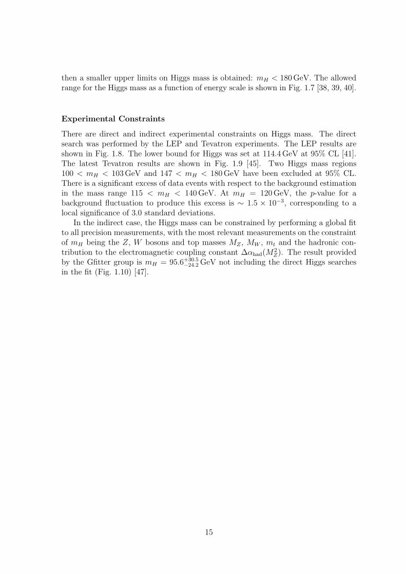
As a result of strong interplay between experimental discoveries and theoretical ad-vances, a successful model to describe the constituents of our world and their interac-tions is founded. This is so called Standard Model (SM) of particle physics. The SMreveals that there are six types of leptons, six types of quarks and their antiparticlesas well. All these together make up of everything in our world. There are four typesof interaction which rule all of the materials in the world, propagated by a set ofbosons. They are strong, electromagnetic, weak and gravity interaction. The gravityinteraction is not incorporated in the SM. In the microscope scale, the gravity in-teraction is however so weak that it is negligible in the study of particle physics. Inthe SM, six leptons are arranged in 3 generations (from left to right in Fig. 1.1) withsimilar physical characteristics [4]). The particles in higher generations have heaviermasses. In each generation, there is one particle with an integer charge (−1) andnone zero mass, while the other lepton is charge neutral, which is called neutrino.Leptons only take part in electroweak interaction. Each lepton has its antiparticlewith an opposite sign charge and same mass.
Quarks, the constituent of baryons and mesons, account for most of the masses inthe world. Similarly six quarks are categorised to three generations, with heavier andheavier masses. Unlike the leptons, quarks have fractional charges. For example, theu, c, t quark have 2/3 charge, and d, s, b have −1/3 charge. As quarks can only existwithin the bounded state in the hadrons, only integer charges can be observed in theexperiment. Quarks will take part in not only the electroweak interaction, but alsothe strong interaction indicated by another kind of charge, color. As the requirementof symmetry in hadrons, there are three colors in all, given the name red, blue andgreen. This assumption was verified by the R value measurement. R is the ratioof the cross section for e+e− annihilation into hadronic final states to the QuantumElectrodynamics (QED) cross section for muon-pair production [5].
In addition, 12 types of bosons propagate the interactions between particles, in-
8
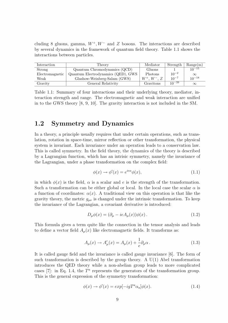
cluding 8 gluons, gamma, W+,W− and Z bosons. The interactions are describedby several dynamics in the framework of quantum field theory. Table 1.1 shows theinteractions between particles.
Interaction Theory Mediator Strength Range(m)Strong Quantum Chromodynamics (QCD) Gluons 1 10−15
Electromagnetic Quantum Electrodynamics (QED), GWS Photons 10−2 ∞Weak Glashow-Weinberg-Salam (GWS) W+, W−, Z 10−7 10−18
Gravity General Relativity Gravitons 10−39 ∞
Table 1.1: Summary of four interactions and their underlying theory, mediator, in-teraction strength and range. The electromagnetic and weak interaction are unifiedin to the GWS theory [8, 9, 10]. The gravity interaction is not included in the SM.
1.2 Symmetry and Dynamics
In a theory, a principle usually requires that under certain operations, such as trans-lation, rotation in space-time, mirror reflection or other transformation, the physicalsystem is invariant. Each invariance under an operation leads to a conservation law.This is called symmetry. In the field theory, the dynamics of the theory is describedby a Lagrangian function, which has an intrisic symmetry, namely the invariance ofthe Lagrangian, under a phase transformation on the complex field:
φ(x) → φ′(x) = eieαφ(x), (1.1)
in which φ(x) is the field, α is a scalar and e is the strength of the transformation.Such a transformation can be either global or local. In the local case the scalar α isa function of coordinates: α(x). A traditional view on this operation is that like thegravity theory, the metric gµν is changed under the intrinsic transformation. To keepthe invariance of the Lagrangian, a covariant derivative is introduced:
Dµφ(x) = (∂µ − ieAµ(x))φ(x) . (1.2)
This formula gives a term quite like the connection in the tensor analysis and leadsto define a vector field Aµ(x) like electromagnetic fields. It transforms as:
Aµ(x) → A′µ(x) = Aµ(x) +
1
e∂µα . (1.3)
It is called gauge field and the invariance is called gauge invariance [6]. The form ofsuch transformation is described by the group theory. A U(1) Abel transformationintroduces the QED theory while a non-abelian group leads to more complicatedcases [7]: in Eq. 1.4, the T a represents the generators of the transformation group.This is the general expression of the symmetry transformation:
φ(x) → φ′(x) = exp[−igT aαa]φ(x). (1.4)
9
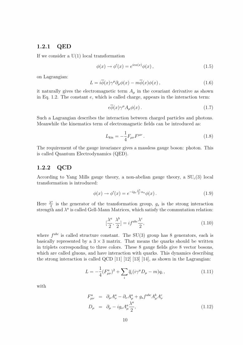
1.2.1 QED
If we consider a U(1) local transformation
φ(x) → φ′(x) = eieα(x)φ(x) , (1.5)
on Lagrangian:L = iφ(x)γµ∂µφ(x) −mφ(x)φ(x) , (1.6)
it naturally gives the electromagnetic term Aµ in the covariant derivative as shownin Eq. 1.2. The constant e, which is called charge, appears in the interaction term:
eφ(x)γµAµφ(x) . (1.7)
Such a Lagrangian describes the interaction between charged particles and photons.Meanwhile the kinematics term of electromagnetic fields can be introduced as:
Lkin = −1
4FµνF
µν . (1.8)
The requirement of the gauge invariance gives a massless gauge boson: photon. Thisis called Quantum Electrodynamics (QED).
1.2.2 QCD
According to Yang Mills gauge theory, a non-abelian gauge theory, a SUc(3) localtransformation is introduced:
φ(x) → φ′(x) = e−igsλa
2αaφ(x) . (1.9)
Here λa
2is the generator of the transformation group, gs is the strong interaction
strength and λa is called Gell-Mann Matrices, which satisfy the commutation relation:
[λa
2,λb
2] = ifabcλ
c
2, (1.10)
where fabc is called structure constant. The SU(3) group has 8 generators, each isbasically represented by a 3 × 3 matrix. That means the quarks should be writtenin triplets corresponding to three colors. These 8 gauge fields give 8 vector bosons,which are called gluons, and have interaction with quarks. This dynamics describingthe strong interaction is called QCD [11] [12] [13] [14], as shown in the Lagrangian:
L = −1
4(F a
µν)2 +
∑
i
qi(iγµDµ −m)qi , (1.11)
with
F aµν = ∂µA
aν − ∂νA
aµ + gsf
abcAbµA
cν
Dµ = ∂µ − igsAaµ
λa
2, (1.12)
10
where q is a triplet, the basic presentation of the SU(3) group, summed over allquark flavours. Due to the non-abelien configuration, the structure constant from thecommutator of generators in the SU(3) group leads to the self interaction of the gaugefield. When the higher order loop diagrams are considered, it is needed to subtract thedivergences by renormalization. The equation of renormalization shows that in theQCD case the strength of interaction is stronger when the distance between particlesincreases. This is the reason why quarks are confined in the hadrons.
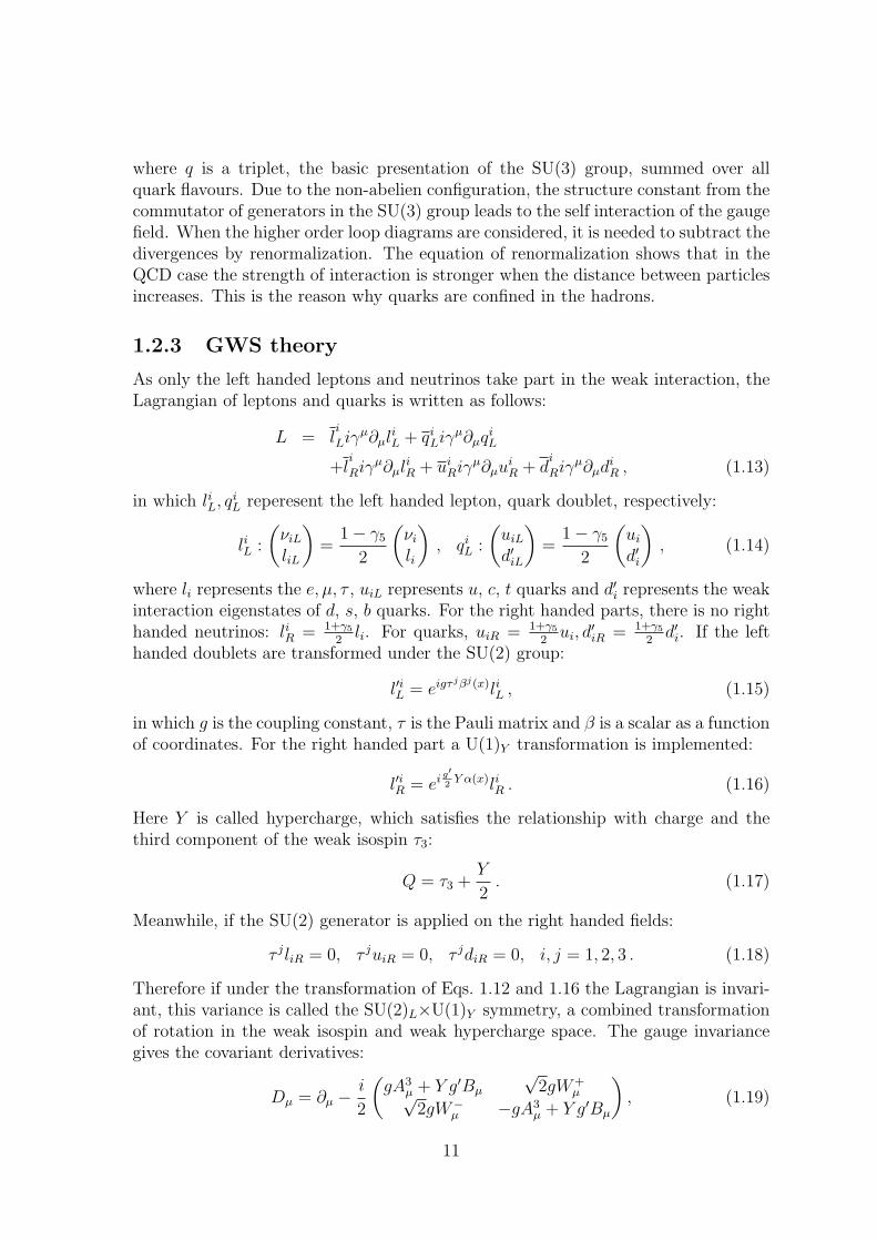
1.2.3 GWS theory
As only the left handed leptons and neutrinos take part in the weak interaction, theLagrangian of leptons and quarks is written as follows:
L = li
Liγµ∂µl
iL + qi
Liγµ∂µq
iL
+li
Riγµ∂µl
iR + ui
Riγµ∂µu
iR + d
i
Riγµ∂µd
iR , (1.13)
in which liL, qiL reperesent the left handed lepton, quark doublet, respectively:
liL :
(
νiL
liL
)
=1 − γ5
2
(
νi
li
)
, qiL :
(
uiL
d′iL
)
=1 − γ5
2
(
ui
d′i
)
, (1.14)
where li represents the e, µ, τ , uiL represents u, c, t quarks and d′i represents the weakinteraction eigenstates of d, s, b quarks. For the right handed parts, there is no righthanded neutrinos: liR = 1+γ5
2li. For quarks, uiR = 1+γ5
2ui, d
′iR = 1+γ5
2d′i. If the left
handed doublets are transformed under the SU(2) group:
l′iL = eigτjβj(x)liL , (1.15)
in which g is the coupling constant, τ is the Pauli matrix and β is a scalar as a functionof coordinates. For the right handed part a U(1)Y transformation is implemented:
l′iR = ei g′
2Y α(x)liR . (1.16)
Here Y is called hypercharge, which satisfies the relationship with charge and thethird component of the weak isospin τ3:
Q = τ3 +Y
2. (1.17)
Meanwhile, if the SU(2) generator is applied on the right handed fields:
τ jliR = 0, τ juiR = 0, τ jdiR = 0, i, j = 1, 2, 3 . (1.18)
Therefore if under the transformation of Eqs. 1.12 and 1.16 the Lagrangian is invari-ant, this variance is called the SU(2)L×U(1)Y symmetry, a combined transformationof rotation in the weak isospin and weak hypercharge space. The gauge invariancegives the covariant derivatives:
Dµ = ∂µ − i
2
(
gA3µ + Y g′Bµ
√2gW+
µ√2gW−
µ −gA3µ + Y g′Bµ
)
, (1.19)
11
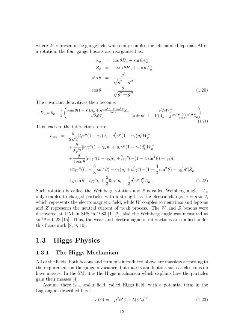
where W represents the gauge field which only couples the left handed leptons. Aftera rotation, the four gauge bosons are reorganised as:
Aµ = cos θBµ + sin θA3µ
Zµ = − sin θBµ + sin θA3µ
sin θ =g′
√
g2 + g′2,
cos θ =g
√
g2 + g′2. (1.20)
The covariant deravitives then become:
Dµ = ∂µ − i
2
(
g sin θ(1 + Y )Aµ + g cos2 θ−Y sin2 θcos θ
Zµ
√2gW+
µ√2gW−
µ g sin θ(−1 + Y )Aµ − g cos2 θ+Y sin2 θcos θ
Zµ
)
.
(1.21)
This leads to the interaction term:
Lint =g
2√
2[liγ
µ(1 − γ5)νi + d′
iγµ(1 − γ5)ui]W
−µ
+g
2√
2[νiγ
µ(1 − γ5)li + uiγµ(1 − γ5)d
′i]W
+µ
+g
4 cos θ[νiγ
µ(1 − γ5)νi + liγµ(−(1 − 4 sin2 θ) + γ5)li
+uiγµ((1 − 8
3sin2 θ) − γ5)ui + d
′
iγµ(−(1 − 4
3sin2 θ) + γ5)d
′i]Zµ
+g sin θ[−liγµli +2
3uiγ
µui −1
3d′
iγµd′i]Aµ . (1.22)
Such rotation is called the Weinberg rotation and θ is called Weinberg angle. Aµ
only couples to charged particles with a strength as the electric charge: e = g sin θ,which represents the electromagnetic field, while W couples to neutrinos and leptonsand Z represents the neutral current of weak process. The W and Z bosons werediscovered at UA1 in SPS in 1983 [1] [2], also the Weinberg angle was measured assin2θ = 0.23 [15]. Thus, the weak and electromagnetic interactions are unified underthis framework [8, 9, 10].
1.3 Higgs Physics
1.3.1 The Higgs Mechanism
All of the fields, both bosons and fermions introduced above are massless according tothe requirement on the gauge invariance, but quarks and leptons such as electrons dohave masses. In the SM, it is the Higgs mechanism which explains how the particlesgain their masses [4].
Assume there is a scalar field, called Higgs field, with a potential term in theLagrangian described here:
V (φ) = −µ2φ⋆φ+ λ(φ⋆φ)2 . (1.23)
12
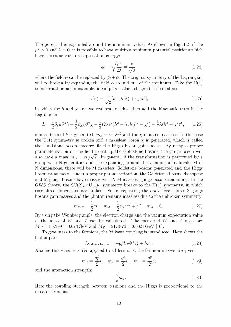
The potential is expanded around the minimum value. As shown in Fig. 1.2, if theµ2 > 0 and λ > 0, it is possible to have multiple minimum potential positions whichhave the same vacuum expectation energy:
φ0 =
√
µ2
2λ≡ v√
2, (1.24)
where the field φ can be replaced by φ0 +φ. The original symmetry of the Lagrangianwill be broken by expanding the field φ around one of the minimum. Take the U(1)transformation as an example, a complex scalar field φ(x) is defined as:
φ(x) =1√2[v + h(x) + iχ(x)], (1.25)
in which the h and χ are two real scalar fields, then add the kinematic term in theLagrangian:
L =1
2∂µh∂
µh+1
2∂µχ∂
µχ− 1
2(2λv2)h2 − λvh(h2 + χ2) − 1
4λ(h2 + χ2)2 , (1.26)
a mass term of h is generated: mh =√
2λv2 and the χ remains massless. In this casethe U(1) symmetry is broken and a massless boson χ is generated, which is calledthe Goldstone boson, meanwhile the Higgs boson gains mass. By using a properparameterisation on the field to eat up the Goldstone bosons, the gauge boson willalso have a mass mA = ev/
√2. In general, if the transformation is performed by a
group with N generators and the expanding around the vacuum point breaks M ofN dimensions, there will be M massless Goldstone bosons generated and the Higgsboson gains mass. Under a proper parameterisation, the Goldstone bosons disappearand M gauge bosons have masses with N-M massless gauge bosons remaining. In theGWS theory, the SU(2)L×U(1)Y symmetry breaks to the U(1) symmetry, in whichcase three dimensions are broken. So by repeating the above procedures 3 gaugebosons gain masses and the photon remains massless due to the unbroken symmetry:
mW± =1
2gv, mZ =
1
2v√
g2 + g′2, mA = 0 . (1.27)
By using the Weinberg angle, the electron charge and the vacuum expectation valuev, the mass of W and Z can be calculated. The measured W and Z mass areMW = 80.399 ± 0.023 GeV and MZ = 91.1876 ± 0.0021 GeV [16].
To give mass to the fermions, the Yukawa coupling is introduced. Here shows thelepton part:
LYukawa lepton = −gLi liRΦ+liL + h.c.. (1.28)
Assume this scheme is also applied to all fermions, the fermion masses are given:
mli ≡gL
i
2v, mdi ≡
gdi
2v, mui ≡
gui
2v, (1.29)
and the interaction strength:
− i
vmf . (1.30)
Here the coupling strength between fermions and the Higgs is proportional to themass of fermions.
13
1.3.2 Higgs Production at the LHC
As one of the main physical purposes for the Large Hadron Collider (LHC) is theHiggs hunting, it is very important to know how the Higgs is produced throughproton-proton process [17]. The Higgs boson is mainly produced from several pro-cesses such as gluon-gluon fusion, vector boson fusion(VBF), vector boson associatedproduction V H(V=W ,Z), and ttH process. The leading Feynman diagrams areshown in Fig. 1.3, in which the gluon-gluon fusion process via a fermion loop has thelargest production cross-section, then follows the pure electroweak process includingthe VBF production. The production cross sections as a function of Higgs mass forthe SM at center-of-mass energies of
√s = 7 TeV and
√s = 8 TeV are shown in
Fig. 1.4. For a model with a fourth generation heavy quarks, the gluon-gluon fusionproduction cross section is significantly enhanced. This is discussed in Chapter 6.
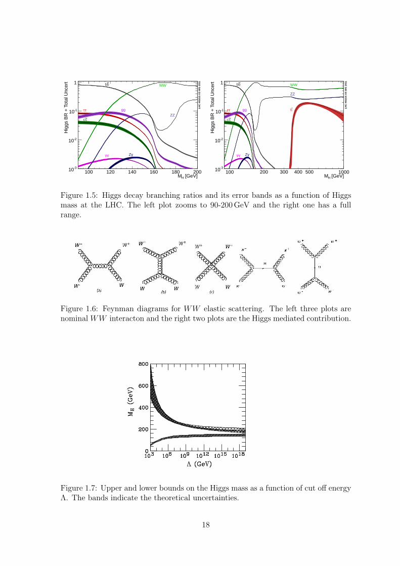
Figure 1.5 shows the SM Higgs decay branching ratio. The WW channel has thedominant branching fraction when the Higgs mass is over 160GeV, therefore the Higgsto the WW channel has the largest sensitivity for the intermediate Higgs mass [21].It also has comparable sensitivity as H → γγ at the low Higgs mass region. The ZZdominates in the high mass range and diphoton dominates in the low mass range. Inthe low Higgs mass region, the Higgs to bb or ττ has larger branching ratio but inthese channels it is very hard to suppress the backgrounds.
1.3.3 Constraints on Higgs Mass
In the following, both the theoretical and direct and indirect experimental constraintson the SM Higgs boson mass are discussed.
Theoretical Constraints
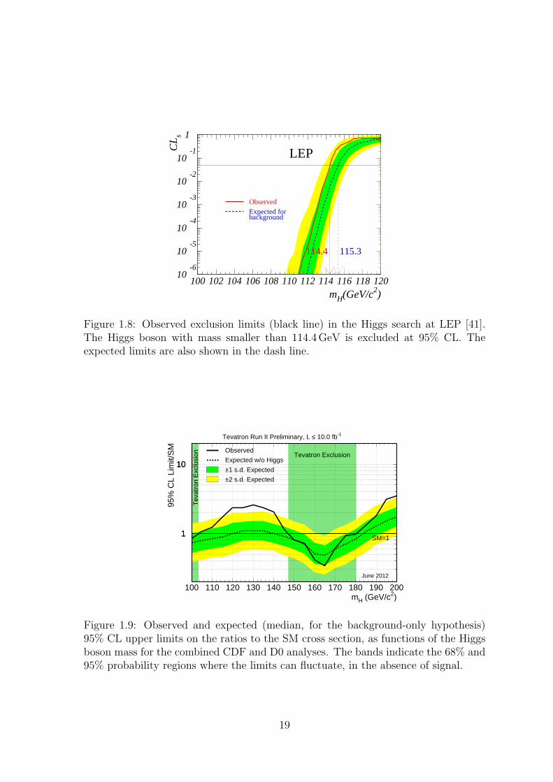
The cross section from the WW elastic scattering in the SM is calculated with anumber of Feynman diagrams shown in Fig. 1.6. If only the left three diagrams areused to calculate the WW scattering cross section, the amplitude for the scattering oflongitudinal W and Z increases with the energy, which finally violates the unitarity ata typical energy of 1.2 TeV. However if the contribution from the Higgs intermediatestate is introduced, shown in the right two diagrams in Fig. 1.6, the unitarity isrestored. This gives constraint on Higgs mass mH < 1 TeV [37].
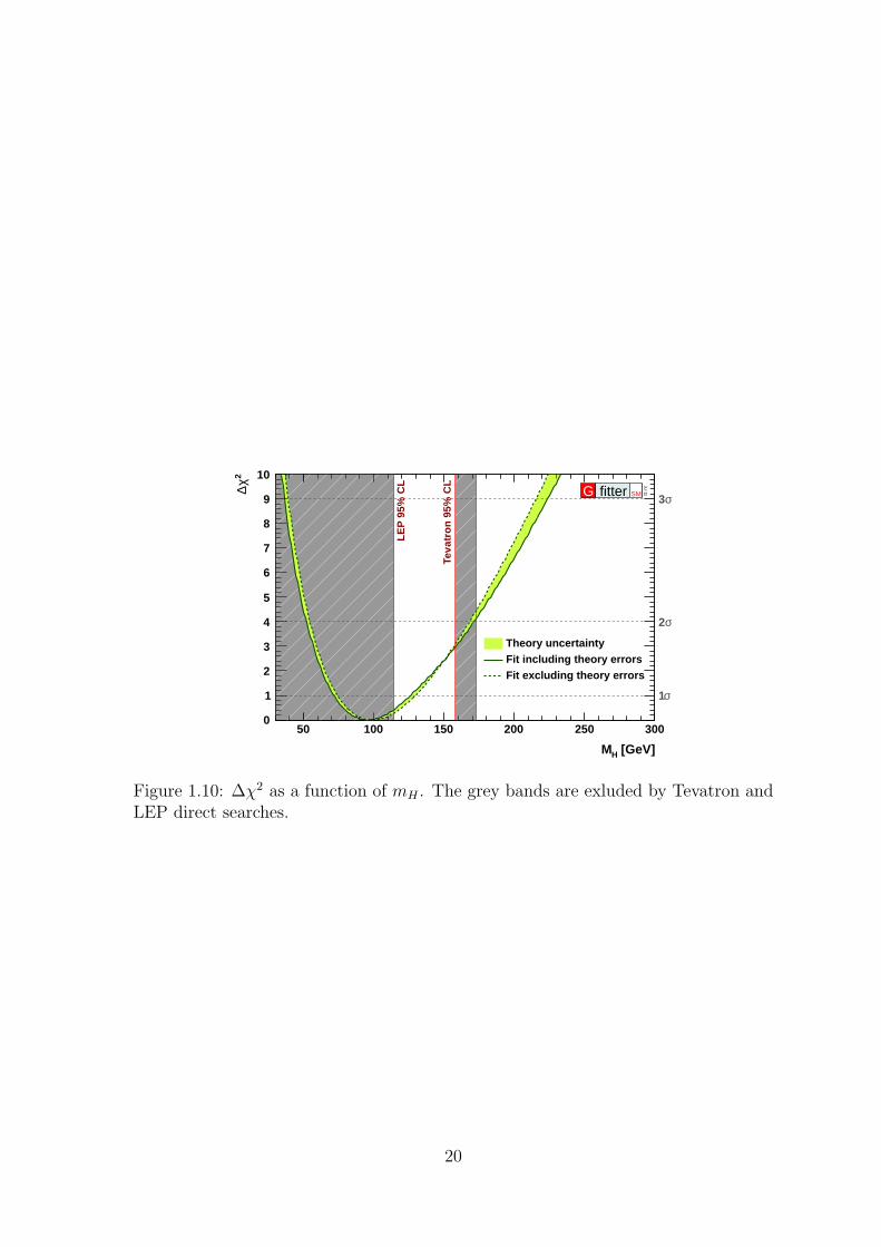
Another theoretical constraint on the Higgs mass is called triviality bound. Byusing the renormalization group equation, the running coupling constant λ is shownas:
d
d lnQλ(Q) =
3λ2
2π2+ O(1) . (1.31)
As mH is a function of λ, if the Higgs mass is very large, the solution to this equationhas a Landau pole. When the Higgs mass is very small, the λ may become negative atlarge energy scale. The former case is called triviality and the latter one the vacuumstability problem. To avoid this, a cut off on the Q should be applied: Q = Λ. If nonew physics, in which the SM is embedded, exsits at the Planck scale mp1 ≃ 1019GeV ,
14
then a smaller upper limits on Higgs mass is obtained: mH < 180 GeV. The allowedrange for the Higgs mass as a function of energy scale is shown in Fig. 1.7 [38, 39, 40].
Experimental Constraints
There are direct and indirect experimental constraints on Higgs mass. The directsearch was performed by the LEP and Tevatron experiments. The LEP results areshown in Fig. 1.8. The lower bound for Higgs was set at 114.4 GeV at 95% CL [41].The latest Tevatron results are shown in Fig. 1.9 [45]. Two Higgs mass regions100 < mH < 103 GeV and 147 < mH < 180 GeV have been excluded at 95% CL.There is a significant excess of data events with respect to the background estimationin the mass range 115 < mH < 140 GeV. At mH = 120 GeV, the p-value for abackground fluctuation to produce this excess is ∼ 1.5 × 10⁻³, corresponding to alocal significance of 3.0 standard deviations.
In the indirect case, the Higgs mass can be constrained by performing a global fitto all precision measurements, with the most relevant measurements on the constraintof mH being the Z, W bosons and top masses MZ , MW , mt and the hadronic con-tribution to the electromagnetic coupling constant ∆αhad(M
2Z). The result provided
by the Gfitter group is mH = 95.6+30.5−24.2 GeV not including the direct Higgs searches
in the fit (Fig. 1.10) [47].
15
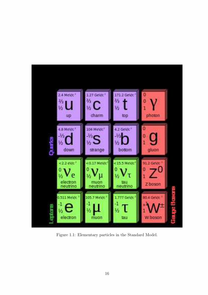
Figure 1.1: Elementary particles in the Standard Model.
16
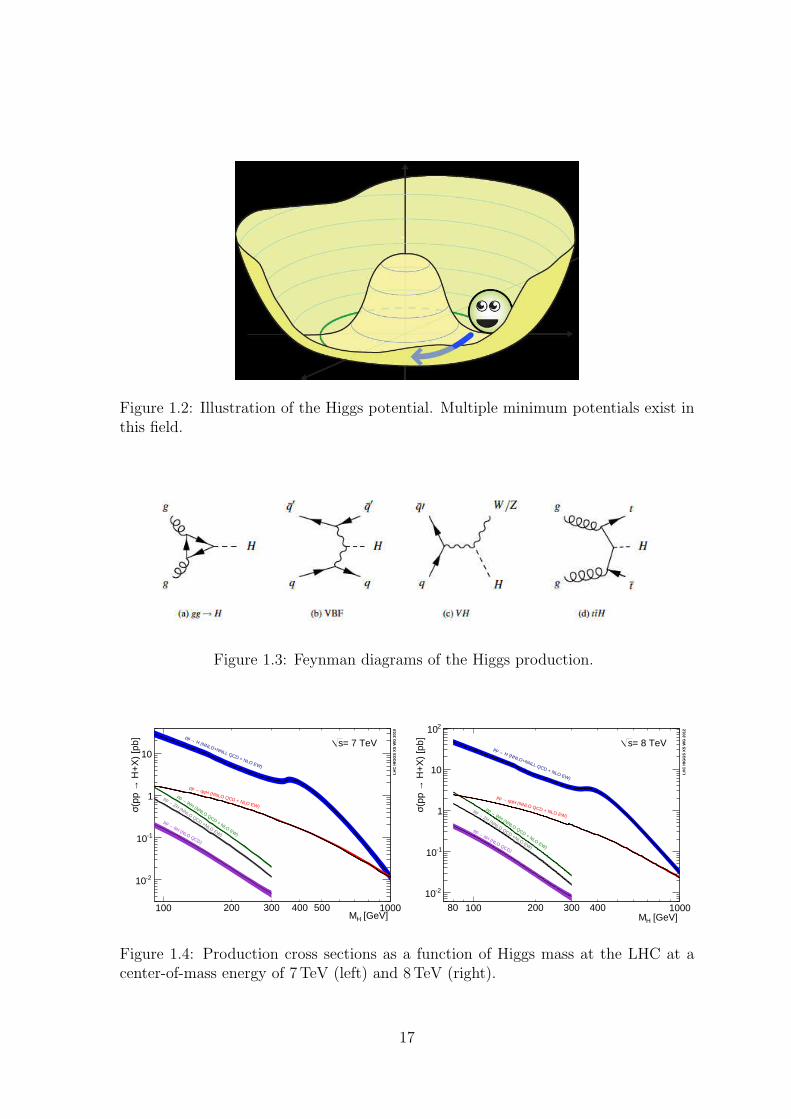
Figure 1.2: Illustration of the Higgs potential. Multiple minimum potentials exist inthis field.
Figure 1.3: Feynman diagrams of the Higgs production.
[GeV] HM100 200 300 400 500 1000
H+
X)
[pb]
→(p
p σ
-210
-110
1
10= 7 TeVs
LH
C H
IGG
S X
S W
G 2
010
H (NNLO+NNLL QCD + NLO EW)
→pp
qqH (NNLO QCD + NLO EW)
→pp
WH (NNLO QCD + NLO EW)
→pp
ZH (NNLO QCD +NLO EW)
→pp
ttH (NLO QCD)
→pp
[GeV] HM80 100 200 300 400 1000
H+
X)
[pb]
→(p
p σ
-210
-110
1
10
210= 8 TeVs
LH
C H
IGG
S X
S W
G 2
012
H (NNLO+NNLL QCD + NLO EW)
→pp
qqH (NNLO QCD + NLO EW)
→pp
WH (NNLO QCD + NLO EW)
→pp
ZH (NNLO QCD +NLO EW)
→pp
ttH (NLO QCD)
→pp
Figure 1.4: Production cross sections as a function of Higgs mass at the LHC at acenter-of-mass energy of 7 TeV (left) and 8 TeV (right).
17
[GeV]HM100 120 140 160 180 200
Hig
gs B
R +
Tot
al U
ncer
t
-310
-210
-110
1
LH
C H
IGG
S X
S W
G 2
011
bb
ττ
cc
gg
γγ γZ
WW
ZZ
[GeV]HM100 200 300 400 500 1000
Hig
gs B
R +
Tot
al U
ncer
t
-310
-210
-110
1
LH
C H
IGG
S X
S W
G 2
011
bb
ττ
cc
ttgg
γγ γZ
WW
ZZ
Figure 1.5: Higgs decay branching ratios and its error bands as a function of Higgsmass at the LHC. The left plot zooms to 90-200 GeV and the right one has a fullrange.
Figure 1.6: Feynman diagrams for WW elastic scattering. The left three plots arenominal WW interacton and the right two plots are the Higgs mediated contribution.
Figure 1.7: Upper and lower bounds on the Higgs mass as a function of cut off energyΛ. The bands indicate the theoretical uncertainties.
18
10-6
10-5
10-4
10-3
10-2
10-1
1
100 102 104 106 108 110 112 114 116 118 120
mH(GeV/c2)
CL
s
114.4 115.3
LEP
ObservedExpected forbackground
Figure 1.8: Observed exclusion limits (black line) in the Higgs search at LEP [41].The Higgs boson with mass smaller than 114.4 GeV is excluded at 95% CL. Theexpected limits are also shown in the dash line.
1
10
100 110 120 130 140 150 160 170 180 190 200
1
10
mH (GeV/c2)
95%
CL
Lim
it/S
M
Tevatron Run II Preliminary, L ≤ 10.0 fb-1
Observed
Expected w/o Higgs
±1 s.d. Expected
±2 s.d. Expected
Tevatron Exclusion
Tev
atro
n E
xclu
sion
SM=1
June 2012
Figure 1.9: Observed and expected (median, for the background-only hypothesis)95% CL upper limits on the ratios to the SM cross section, as functions of the Higgsboson mass for the combined CDF and D0 analyses. The bands indicate the 68% and95% probability regions where the limits can fluctuate, in the absence of signal.
19
[GeV]HM
50 100 150 200 250 300
2 χ∆
0
1
2
3
4
5
6
7
8
9
10
LEP
95%
CL
Teva
tron
95%
CL
σ1
σ2
σ3
Theory uncertaintyFit including theory errorsFit excluding theory errors
G fitter SM
Jul 11
Figure 1.10: ∆χ2 as a function of mH . The grey bands are exluded by Tevatron andLEP direct searches.
20
Chapter 2
The Large Hadron Collider andATLAS Detector
2.1 The Large Hadron Collider
The Large Hadron Collider (LHC) [48] is the largest experimental device ever built inthe world. It is located across the border of Swiss and France, mainly in a 90 metersdepth tunnel with 27 km perimeter, which was used by the former LEP (Large Elec-tron Positron Collider). Unlike an electron-positron collider or a proton-antiprotoncollider, the LHC is designed as a proton-proton collider to achieve a very high energybeam with relatively lower synchrotron radiation in the arcs. It is designed to havea nominal center-of-mass energy of 14 TeV with a peak instantaneous luminosity of1034 cm−2s−1. To achieve such high energy in the circular tunnel, the high qualifiedbending superconducting magnets and the state of the art technology are required.The classical Nb-Ti superconducting magnets were used in a two-in-one mode in thenarrow LEP tunnel. The magnets are cooled below 2 K, by using the superfluid he-lium, to provide up to 8.5 T central magnetic field. Besides the energy, the otherimportant feature of the LHC is its high luminosity, which is defined as [58]:
L =1
4π
N1 ·N2 · Fσx · σy · t
(2.1)
in whichN1, N2 are the numbers of protons in the two colliding bunches, σx, σy charac-terize the widths of horizontal and vertical beam profile, t is the time interval betweenbunches and F is the geometric luminosity reduction factor due to the crossing angleat the interaction point. According to the LHC design, the typical number of protonsper bunch is 1.15 × 10¹¹, the time interval between bunches is 25 ns. The numberof interactions per bunch crossing is about 25 which is dominated by soft elastic ppcollisions. In addition, the LHC can provide heavy ion collision, such as lead ion,with the design luminosity of 1027 cm−2s−1 at 2.8 TeV per beam energy.
Four main detectors and two small detectors are installed around the LHC (Fig. 2.1).They are: ALICE (A Large Ion Collider Experiment) [49], ATLAS (A Toroidal LHCApparatuS) [50], CMS (Compact Muon Solenoid) [51], LHCb (Large Hadron Col-
21
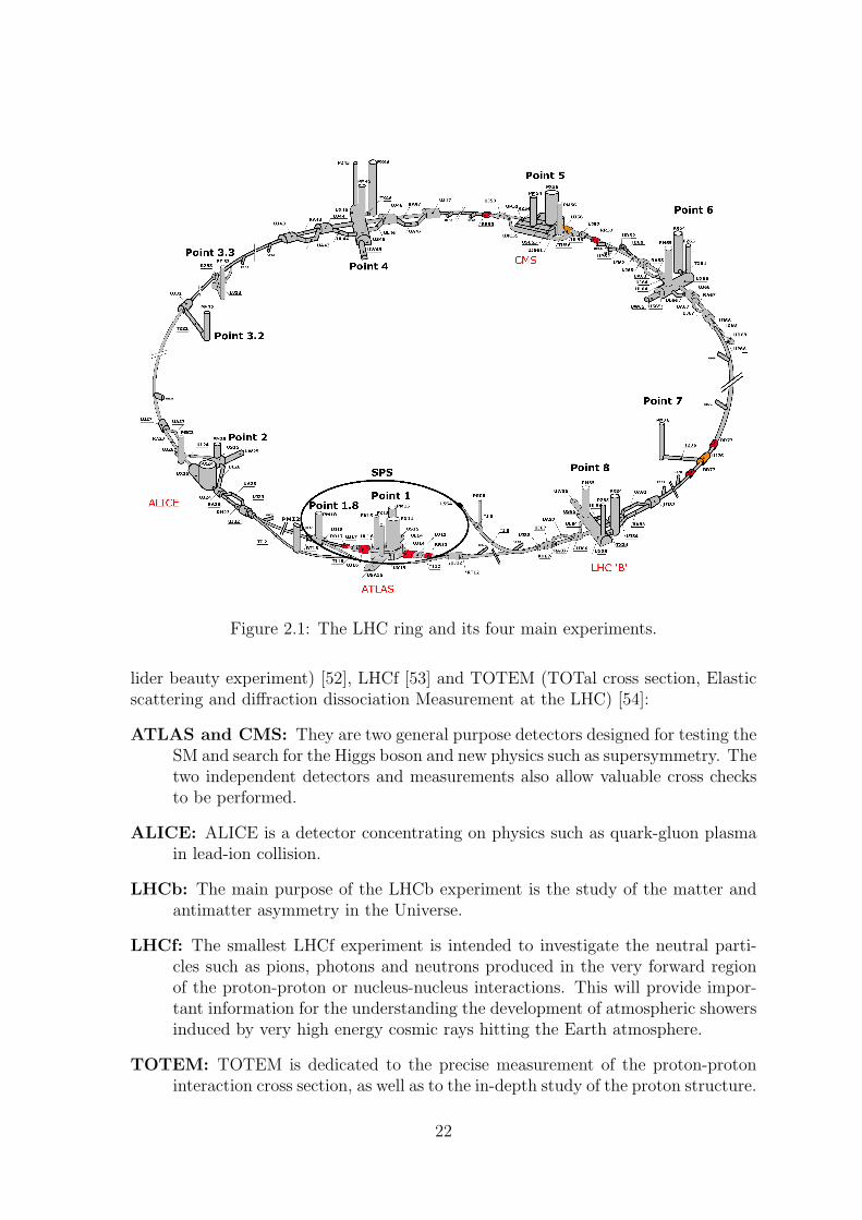
Figure 2.1: The LHC ring and its four main experiments.
lider beauty experiment) [52], LHCf [53] and TOTEM (TOTal cross section, Elasticscattering and diffraction dissociation Measurement at the LHC) [54]:
ATLAS and CMS: They are two general purpose detectors designed for testing theSM and search for the Higgs boson and new physics such as supersymmetry. Thetwo independent detectors and measurements also allow valuable cross checksto be performed.
ALICE: ALICE is a detector concentrating on physics such as quark-gluon plasmain lead-ion collision.
LHCb: The main purpose of the LHCb experiment is the study of the matter andantimatter asymmetry in the Universe.
LHCf: The smallest LHCf experiment is intended to investigate the neutral parti-cles such as pions, photons and neutrons produced in the very forward regionof the proton-proton or nucleus-nucleus interactions. This will provide impor-tant information for the understanding the development of atmospheric showersinduced by very high energy cosmic rays hitting the Earth atmosphere.
TOTEM: TOTEM is dedicated to the precise measurement of the proton-protoninteraction cross section, as well as to the in-depth study of the proton structure.
22
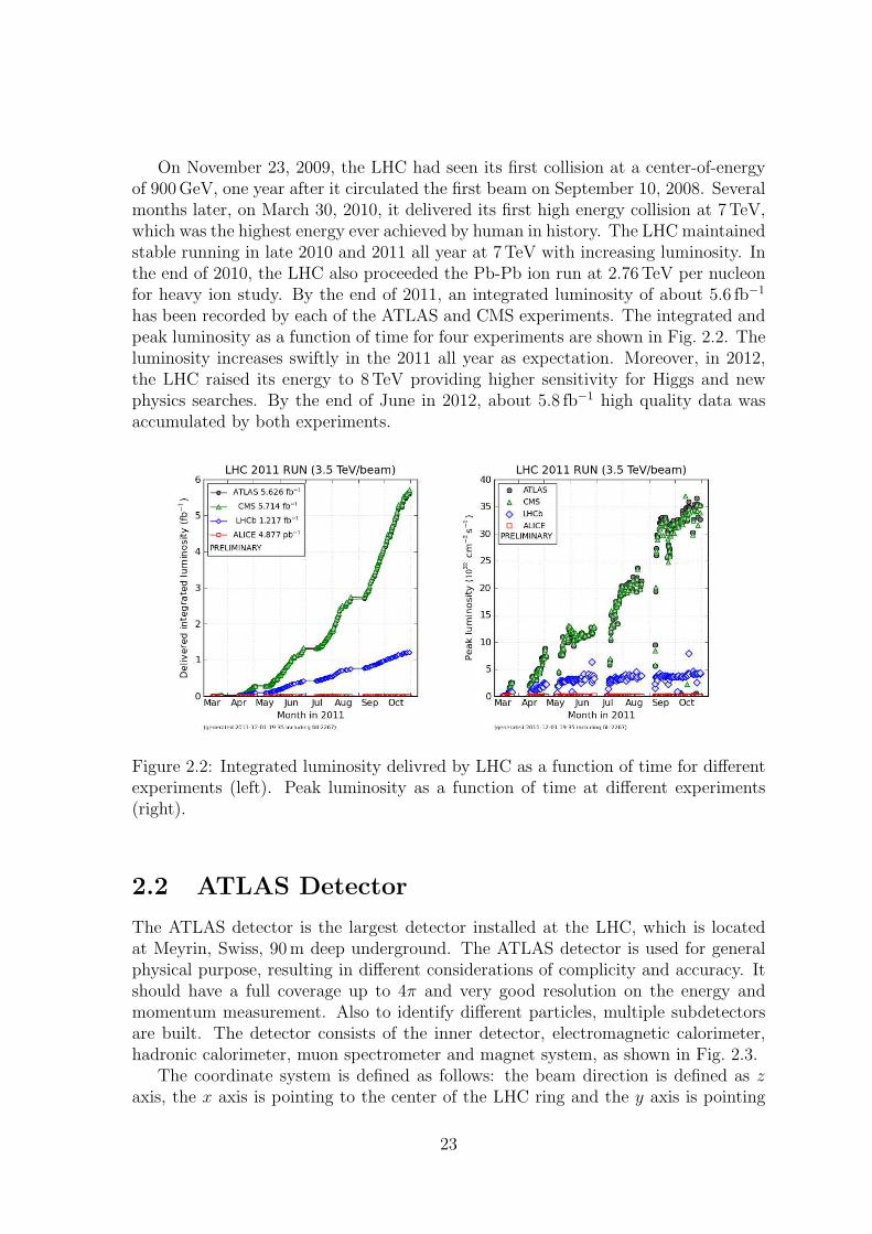
On November 23, 2009, the LHC had seen its first collision at a center-of-energyof 900 GeV, one year after it circulated the first beam on September 10, 2008. Severalmonths later, on March 30, 2010, it delivered its first high energy collision at 7TeV,which was the highest energy ever achieved by human in history. The LHC maintainedstable running in late 2010 and 2011 all year at 7 TeV with increasing luminosity. Inthe end of 2010, the LHC also proceeded the Pb-Pb ion run at 2.76TeV per nucleonfor heavy ion study. By the end of 2011, an integrated luminosity of about 5.6 fb−1
has been recorded by each of the ATLAS and CMS experiments. The integrated andpeak luminosity as a function of time for four experiments are shown in Fig. 2.2. Theluminosity increases swiftly in the 2011 all year as expectation. Moreover, in 2012,the LHC raised its energy to 8 TeV providing higher sensitivity for Higgs and newphysics searches. By the end of June in 2012, about 5.8 fb−1 high quality data wasaccumulated by both experiments.
Figure 2.2: Integrated luminosity delivred by LHC as a function of time for differentexperiments (left). Peak luminosity as a function of time at different experiments(right).
2.2 ATLAS Detector
The ATLAS detector is the largest detector installed at the LHC, which is locatedat Meyrin, Swiss, 90 m deep underground. The ATLAS detector is used for generalphysical purpose, resulting in different considerations of complicity and accuracy. Itshould have a full coverage up to 4π and very good resolution on the energy andmomentum measurement. Also to identify different particles, multiple subdetectorsare built. The detector consists of the inner detector, electromagnetic calorimeter,hadronic calorimeter, muon spectrometer and magnet system, as shown in Fig. 2.3.
The coordinate system is defined as follows: the beam direction is defined as zaxis, the x axis is pointing to the center of the LHC ring and the y axis is pointing
23
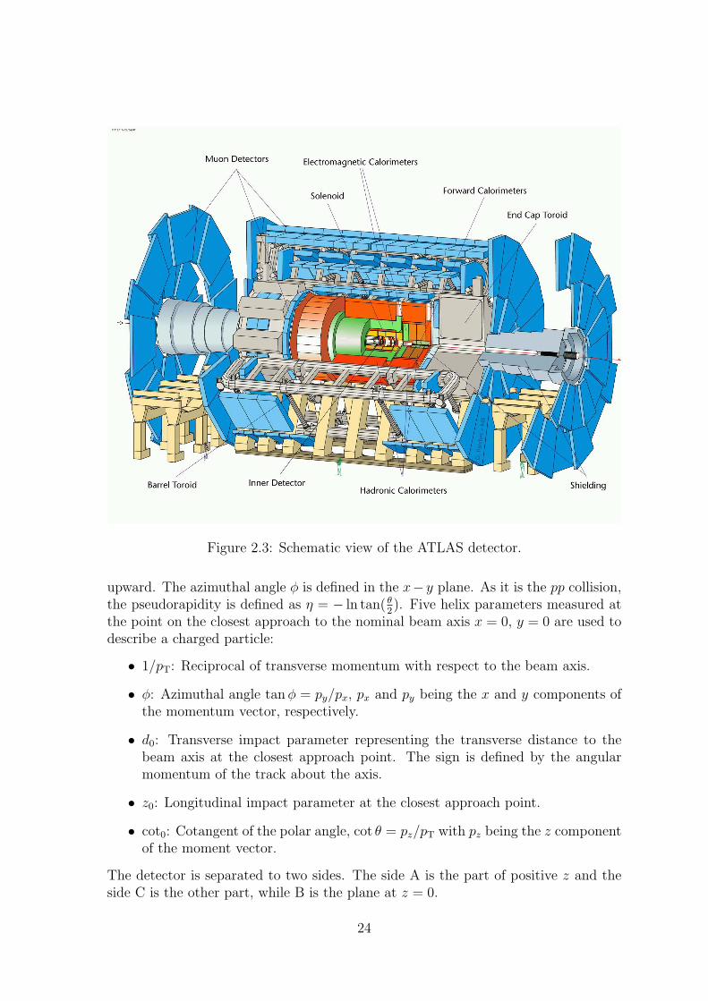
Figure 2.3: Schematic view of the ATLAS detector.
upward. The azimuthal angle φ is defined in the x− y plane. As it is the pp collision,the pseudorapidity is defined as η = − ln tan( θ
2). Five helix parameters measured at
the point on the closest approach to the nominal beam axis x = 0, y = 0 are used todescribe a charged particle:
• 1/pT: Reciprocal of transverse momentum with respect to the beam axis.
• φ: Azimuthal angle tanφ = py/px, px and py being the x and y components ofthe momentum vector, respectively.
• d0: Transverse impact parameter representing the transverse distance to thebeam axis at the closest approach point. The sign is defined by the angularmomentum of the track about the axis.
• z0: Longitudinal impact parameter at the closest approach point.
• cot0: Cotangent of the polar angle, cot θ = pz/pT with pz being the z componentof the moment vector.
The detector is separated to two sides. The side A is the part of positive z and theside C is the other part, while B is the plane at z = 0.
24
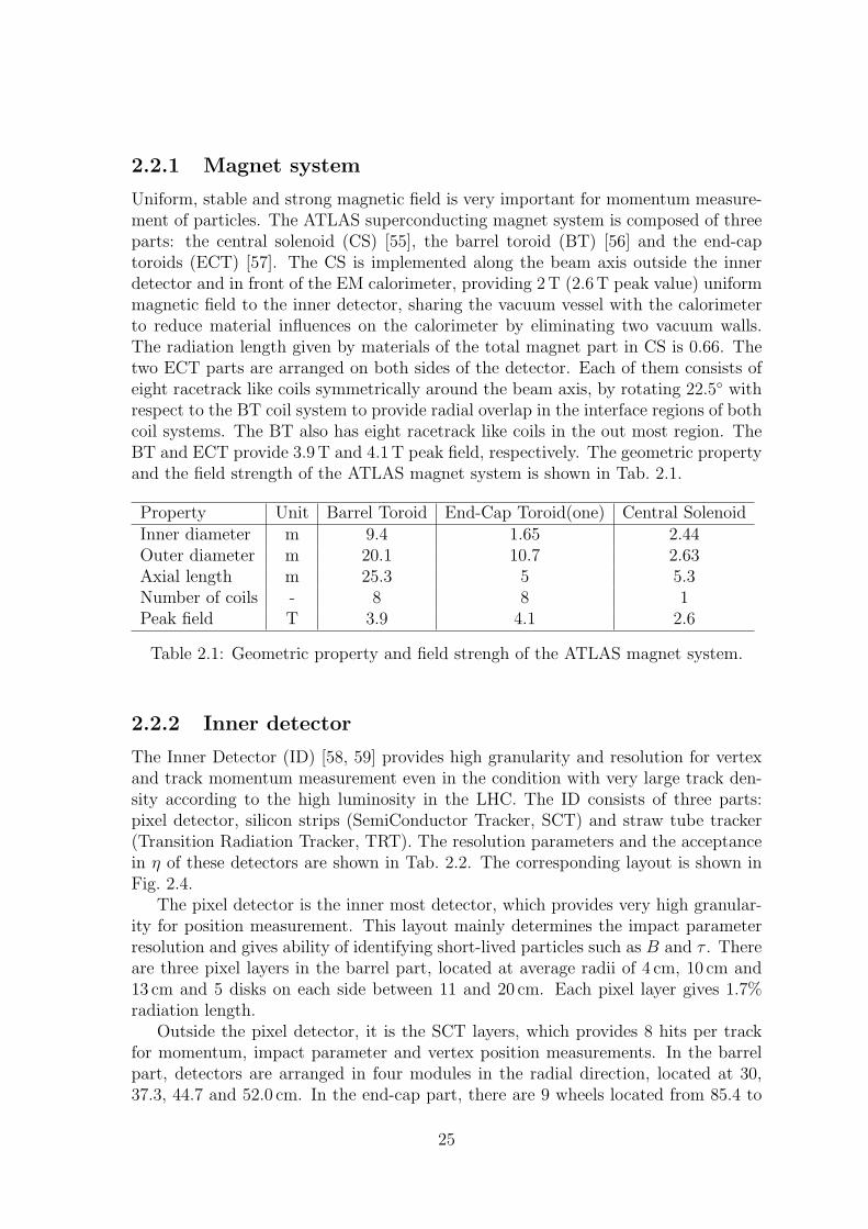
2.2.1 Magnet system
Uniform, stable and strong magnetic field is very important for momentum measure-ment of particles. The ATLAS superconducting magnet system is composed of threeparts: the central solenoid (CS) [55], the barrel toroid (BT) [56] and the end-captoroids (ECT) [57]. The CS is implemented along the beam axis outside the innerdetector and in front of the EM calorimeter, providing 2T (2.6 T peak value) uniformmagnetic field to the inner detector, sharing the vacuum vessel with the calorimeterto reduce material influences on the calorimeter by eliminating two vacuum walls.The radiation length given by materials of the total magnet part in CS is 0.66. Thetwo ECT parts are arranged on both sides of the detector. Each of them consists ofeight racetrack like coils symmetrically around the beam axis, by rotating 22.5◦ withrespect to the BT coil system to provide radial overlap in the interface regions of bothcoil systems. The BT also has eight racetrack like coils in the out most region. TheBT and ECT provide 3.9 T and 4.1 T peak field, respectively. The geometric propertyand the field strength of the ATLAS magnet system is shown in Tab. 2.1.
Property Unit Barrel Toroid End-Cap Toroid(one) Central SolenoidInner diameter m 9.4 1.65 2.44Outer diameter m 20.1 10.7 2.63Axial length m 25.3 5 5.3Number of coils - 8 8 1Peak field T 3.9 4.1 2.6
Table 2.1: Geometric property and field strengh of the ATLAS magnet system.
2.2.2 Inner detector
The Inner Detector (ID) [58, 59] provides high granularity and resolution for vertexand track momentum measurement even in the condition with very large track den-sity according to the high luminosity in the LHC. The ID consists of three parts:pixel detector, silicon strips (SemiConductor Tracker, SCT) and straw tube tracker(Transition Radiation Tracker, TRT). The resolution parameters and the acceptancein η of these detectors are shown in Tab. 2.2. The corresponding layout is shown inFig. 2.4.
The pixel detector is the inner most detector, which provides very high granular-ity for position measurement. This layout mainly determines the impact parameterresolution and gives ability of identifying short-lived particles such as B and τ . Thereare three pixel layers in the barrel part, located at average radii of 4 cm, 10 cm and13 cm and 5 disks on each side between 11 and 20 cm. Each pixel layer gives 1.7%radiation length.
Outside the pixel detector, it is the SCT layers, which provides 8 hits per trackfor momentum, impact parameter and vertex position measurements. In the barrelpart, detectors are arranged in four modules in the radial direction, located at 30,37.3, 44.7 and 52.0 cm. In the end-cap part, there are 9 wheels located from 85.4 to
25
System Position Resolution σ(µm) η coveragePixels 1 removable barrel layer (B-layer) Rφ = 12, z = 66 ±2.5
2 barrel layer Rφ = 12, z = 66 ±1.75 end-cap disks on each side Rφ = 12, R = 77 1.7 − 2.5
Silicon strips 4 barrel layers Rφ = 16, z = 580 ±1.49 end-cap wheels on each side Rφ = 16, R = 580 1.4 − 2.5
TRT Axial barrel straws 170 (per straw) ±0.7Radial end-cap straws 170 (per straw) 0.71.4 − 2.5
Table 2.2: Resolution parameters and η acceptance of the ID subdetectors.
Figure 2.4: Structure of the inner detector.
26
272.0 cm in z direction. The total radiation length from all strips and other materialsgives 2.16% at η = 0 and 1.58% − 2.32% for 9 wheels. There are 6.2 million readoutchannels in all.
Then follows the TRT, which is a set of straw tubes like capacitors placed within30µm diameter gold-plated W-Re sense wires and filled with mixture gas: 70%Xe ,20% CO2 and 10% CF4. The maximum length of the straw is 144 cm and the diameteris 4 mm. The barrel part covers the radii from 56 to 107 cm, while the end-cap partcovers the radii from 64 to 103 cm with 14 wheels nearest the interaction point andthen extended to 48 cm in the last four wheels, which provides an acceptance in theregion |η| < 2.0. There are 370 000 straw tubes in total. A typical track goes across36 straws at least in the transverse plane. The TRT also provides the separationbetween electrons and pions by using the different behavior of emission of transitionradiation photons [60]. For a several GeV case, electrons deposition in 7 straws underthe TRT threshold is around 7 keV, while pions can achieve such energy in one or twostraws.
The most relevant performance in the inner detector concerns the following as-pects: measurements of vertices, the track parameters and the track reconstructionefficiency. The latter is related to the reconstruction of leptons, the isolation per-formance and the pT calibration. The distributions of transverse impact parameterand longitudinal impact parameter multiplied by sin(θ) are shown in Fig. 2.5 [61].Figure 2.6 shows the expected track reconstruction efficiency measured as a functionof η and pT [61], in which the track reconstruction efficiency in the central region andwith high pT reaches 80%. The measured resolution for vertex position using 2011data is shown in Fig. 2.7 [62], agreement between data and MC is obtained in theseplots.
[mm]0d
-5 -4 -3 -2 -1 0 1 2 3 4 5
sel
N
2
4
6
8
10
12
14
16
610×
MC ND
Data 2010
ATLAS
| < 2.5η 2, | ≥ chn < 500 MeV
Tp100 <
= 7 TeVs
[mm]0
d
-5 -4 -3 -2 -1 0 1 2 3 4 5
sel
N
610
710
[mm]θsin0z
-5 -4 -3 -2 -1 0 1 2 3 4 5
sel
N
2
4
6
8
10
12
14
16610×
MC ND
Data 2010
ATLAS
| < 2.5η 2, | ≥ chn < 500 MeV
Tp100 <
= 7 TeVs
[mm]θsin0z
-5 -4 -3 -2 -1 0 1 2 3 4 5
sel
N
610
710
Figure 2.5: Comparison between data and simulation at√s = 7TeV for tracks with
transverse momentum between 100 and 500 MeV: the transverse impact parameter(left) and longitudinal impact parameter multiplied by sin(θ) (right). The insertsfor the impact parameter plots show the log-scale plots. The pT distribution of thetracks in non-diffractive (ND) MC is re-weighted to match the data and the numberof events is scaled to the data.
27
η
-2 -1 0 1 2
trk
ε
0.3
0.4
0.5
0.6
0.7
0.8
0.9ATLAS Simulation
| < 2.5η > 100 MeV, | T
p 2, ≥ chn
= 7 TeVs
MC ND
η
-2 -1 0 1 2
trk
ε
0.3
0.4
0.5
0.6
0.7
0.8
0.9
[GeV]T
p1 10
trk
ε
0
0.1
0.2
0.3
0.4
0.5
0.6
0.7
0.8
0.9
1ATLAS Simulation
| < 2.5η > 100 MeV, | T
p 2, ≥ chn
= 7 TeVs
MC ND
[GeV]T
p1 10
trk
ε
0
0.1
0.2
0.3
0.4
0.5
0.6
0.7
0.8
0.9
1
Figure 2.6: Track reconstruction efficiency based on non-diffractive (ND) MC shownas a function of η (left) and pT (right). The statistical errors are shown as black lines,the total errors as green shaded areas. All distributions are shown at
√s = 7TeV for
number of charged particles greater than 2, pT > 100 MeV, |η| < 2.5.
2.2.3 Calorimeter
The ATLAS calorimeter [63, 64] consists of two parts, the electromagnetic (EM)calorimeter and the hadronic one. The EM calorimeter is very important for preciseenergy measurement of photons and electrons while the hadronic calorimeter willprovide the jets energy information.
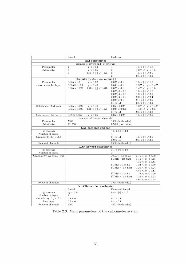
The EM calorimeter consists of the barrel part (EMB) (|η| < 1.475) and two endcap parts (EMEC) on each side of the barrel (|η| < 3.2). The EM calorimeters aresampling calorimeter using liquid argon as active material, filled in 2.09mm gapsbetween the lead absorber. The calorimeter is designed as accordion shape to provideredundant coverage in the φ direction. It consists of three layers and a presampleroutside the cryostat to correct energy lost in the material in front of calorimeter, asshown in Fig. 2.8. Each layer of the EM calorimeter has thousands of cells as theminimum units for energy measurement and providing high granularity (δη× δφ), asshown in Tab. 2.3. The front layer (sampling 1) has the best granularity in η whilethe middle layer (sampling 2) provides the best φ positioning. The radiation lengthin the barrel part is 24X0, dominated by the middle layer. In the end-cap region theradiation length is 26X0.
The energy in the EM calorimeter is calculated by measuring ADC signals in eachcell and summed by layers after calibration, as shown:
Etot = wglob(wpsEps + Efront + Emid + Eback) . (2.2)
The presampler weight wps is used to optimise the energy resolution. The correspond-ing energy resolution is generally expressed as:
σ
E=
a
E⊕ b√
E⊕ c (2.3)
28
5 10 15 20 25 30 35 40 45 50
X V
erte
x R
esol
utio
n [m
m]
-210
-110
1
Data 2011, Random Trigger
Minimum Bias MCATLAS Preliminary
Number of tracks
5 10 15 20 25 30 35 40 45 50
Dat
a / M
C
0.8
0.9
1
1.1
1.2
1.3
5 10 15 20 25 30 35 40 45 50
Y V
erte
x R
esol
utio
n [m
m]
-210
-110
1
Data 2011, Random Trigger
Minimum Bias MCATLAS Preliminary
Number of tracks
5 10 15 20 25 30 35 40 45 50
Dat
a / M
C
0.8
0.9
1
1.1
1.2
1.3
5 10 15 20 25 30 35 40 45 50
Z V
erte
x R
esol
utio
n [m
m]
-210
-110
1
Data 2011, Random Trigger
Minimum Bias MCATLAS Preliminary
Number of tracks
5 10 15 20 25 30 35 40 45 50
Dat
a / M
C
0.8
0.9
1
1.1
1.2
1.3
Figure 2.7: Measured resolution of vertex position as a function of number of tracksattached to this vertex. The resolution is shown in x (top), y (middle), z (bottom).
29
Barrel End-cap
EM calorimeter
Number of layers and |η| coveragePresampler 1 |η| < 1.52 1 1.5 < |η| < 1.8Calorimeter 3 |η| < 1.35 2 1.375 < |η| < 1.5
2 1.35 < |η| < 1.475 3 1.5 < |η| < 2.52 2.5 < |η| < 3.2
Granularity ∆η × ∆φ versus |η|Presampler 0.025 × 0.1 |η| < 1.52 0.025 × 0.1 1.5 < |η| < 1.8
Calorimeter 1st layer 0.025/8 × 0.1 |η| < 1.40 0.050 × 0.1 1.375 < |η| < 1.4250.025 × 0.025 1.40 < |η| < 1.475 0.025 × 0.1 1.425 < |η| < 1.5
0.025/8 × 0.1 1.5 < |η| < 1.80.025/6 × 0.1 1.8 < |η| < 2.00.025/4 × 0.1 2.0 < |η| < 2.40.025 × 0.1 2.4 < |η| < 2.50.1 × 0.1 2.5 < |η| < 3.2
Calorimeter 2nd layer 0.025 × 0.025 |η| < 1.40 0.05 × 0.025 1.375 < |η| < 1.4250.075 × 0.025 1.40 < |η| < 1.475 0.025 × 0.025 1.425 < |η| < 2.5
0.1 × 0.1 2.5 < |η| < 3.2Calorimeter 3rd layer 0.05 × 0.025 |η| < 1.35 0.05 × 0.025 1.5 < |η| < 2.5
Number of readout channelsPresampler 7808 1536 (both sides)Calorimeter 101760 62208 (both sides)
LAr hadronic end-cap
|η| coverage 1.5 < |η| < 3.2Number of layers 4
Granularity ∆η × ∆φ 0.1 × 0.1 1.5 < |η| < 2.50.2 × 0.2 2.5 < |η| < 3.2
Readout channels 5632 (both sides)
LAr forward calorimeter
|η| coverage 3.1 < |η| < 4.9Number of layers 3
Granularity ∆x × ∆y (cm) FCal1 : 3.0 × 2.6 3.15 < |η| < 4.30FCal1:∼ 4× finer 3.10 < |η| < 3.15
4.30 < |η| < 4.83FCal2: 3.3 × 4.2 3.24 < |η| < 4.50FCal2: ∼ 4× finer 3.20 < |η| < 3.24
4.50 < |η| < 4.81FCal3: 3.3 × 4.2 3.32 < |η| < 4.60FCal3: ∼ 4× finer 3.29 < |η| < 3.32
4.60 < |η| < 4.75Readout channels 3524 (both sides)
Scintillator tile calorimeter
Barrel Extended barrel|η| coverage |η| < 1.0 0.8 < |η| < 1.7
Number of layers 3 3Granularity ∆η × ∆φ 0.1 × 0.1 0.1 × 0.1
Last layer 0.2 × 0.1 0.2 × 0.1Readout channels 5760 4092 (both sides)
Table 2.3: Main parameters of the calorimeter system.
30
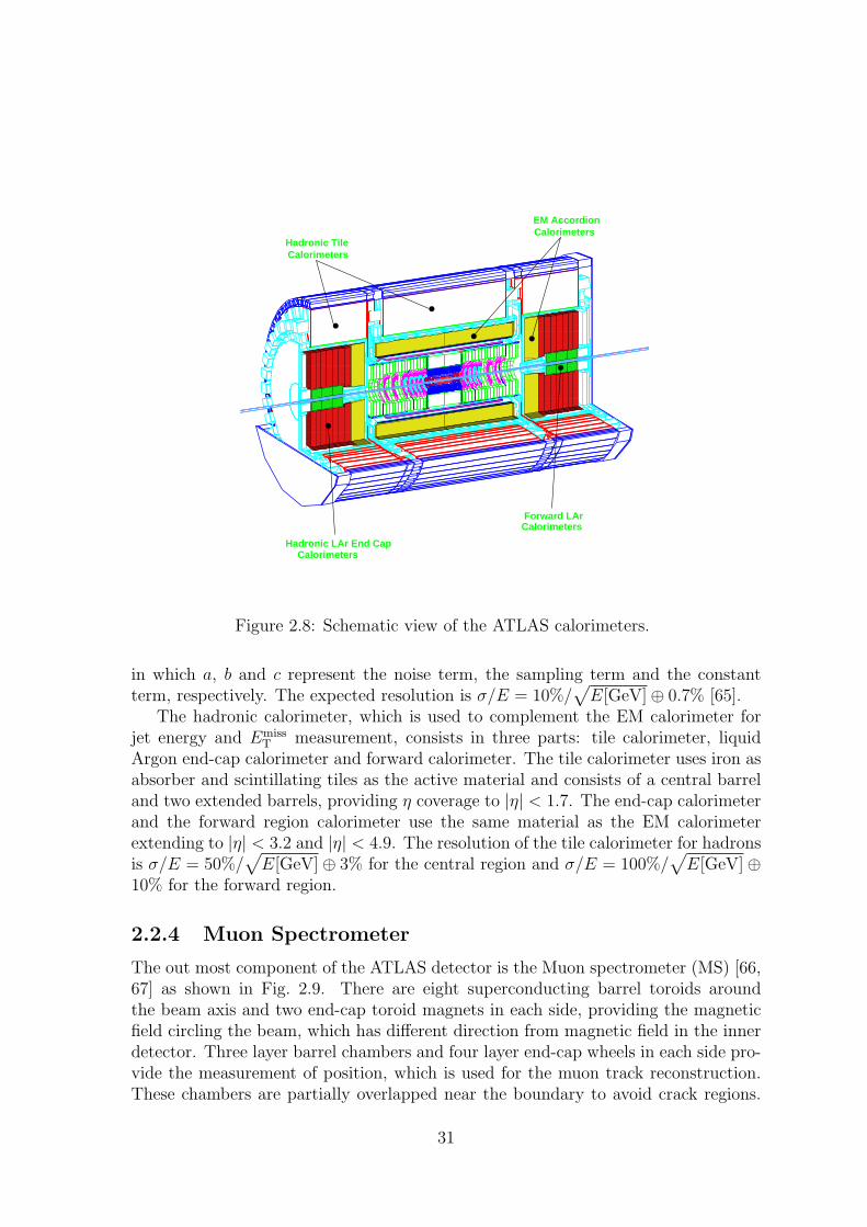
Calorimeters
Calorimeters
Calorimeters
Calorimeters
Hadronic Tile
EM Accordion
Forward LAr
Hadronic LAr End Cap
Figure 2.8: Schematic view of the ATLAS calorimeters.
in which a, b and c represent the noise term, the sampling term and the constantterm, respectively. The expected resolution is σ/E = 10%/
√
E[GeV] ⊕ 0.7% [65].The hadronic calorimeter, which is used to complement the EM calorimeter for
jet energy and EmissT measurement, consists in three parts: tile calorimeter, liquid
Argon end-cap calorimeter and forward calorimeter. The tile calorimeter uses iron asabsorber and scintillating tiles as the active material and consists of a central barreland two extended barrels, providing η coverage to |η| < 1.7. The end-cap calorimeterand the forward region calorimeter use the same material as the EM calorimeterextending to |η| < 3.2 and |η| < 4.9. The resolution of the tile calorimeter for hadronsis σ/E = 50%/
√
E[GeV] ⊕ 3% for the central region and σ/E = 100%/√
E[GeV] ⊕10% for the forward region.
2.2.4 Muon Spectrometer
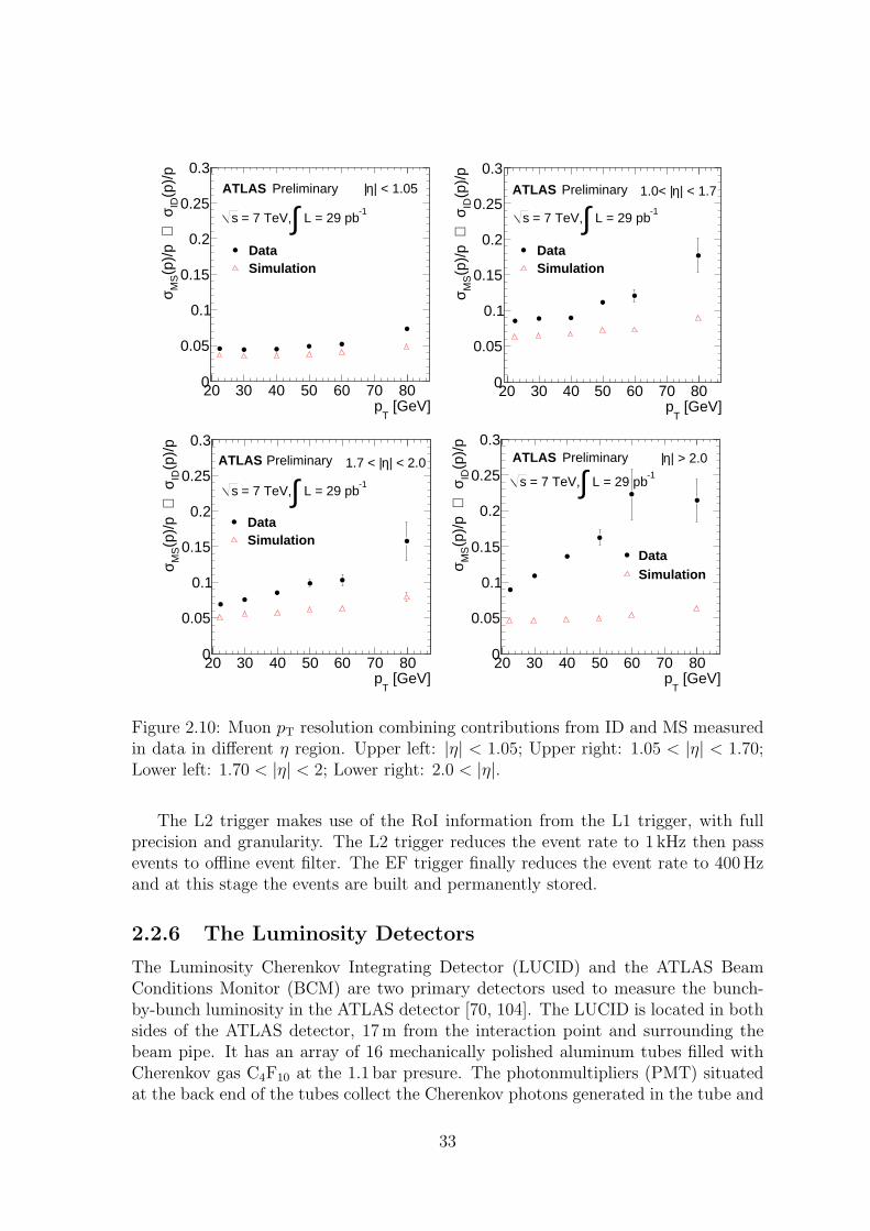
The out most component of the ATLAS detector is the Muon spectrometer (MS) [66,67] as shown in Fig. 2.9. There are eight superconducting barrel toroids aroundthe beam axis and two end-cap toroid magnets in each side, providing the magneticfield circling the beam, which has different direction from magnetic field in the innerdetector. Three layer barrel chambers and four layer end-cap wheels in each side pro-vide the measurement of position, which is used for the muon track reconstruction.These chambers are partially overlapped near the boundary to avoid crack regions.
31
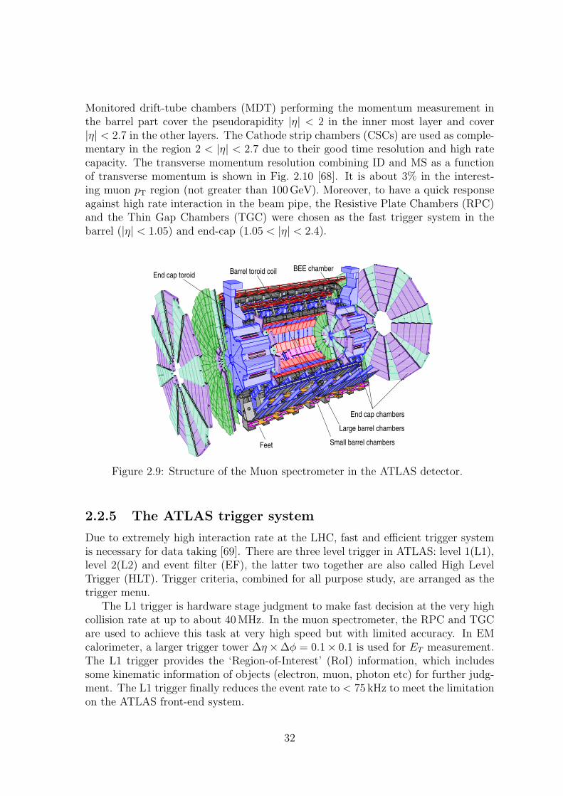
Monitored drift-tube chambers (MDT) performing the momentum measurement inthe barrel part cover the pseudorapidity |η| < 2 in the inner most layer and cover|η| < 2.7 in the other layers. The Cathode strip chambers (CSCs) are used as comple-mentary in the region 2 < |η| < 2.7 due to their good time resolution and high ratecapacity. The transverse momentum resolution combining ID and MS as a functionof transverse momentum is shown in Fig. 2.10 [68]. It is about 3% in the interest-ing muon pT region (not greater than 100GeV). Moreover, to have a quick responseagainst high rate interaction in the beam pipe, the Resistive Plate Chambers (RPC)and the Thin Gap Chambers (TGC) were chosen as the fast trigger system in thebarrel (|η| < 1.05) and end-cap (1.05 < |η| < 2.4).
End cap toroid Barrel toroid coil BEE chamber
Large barrel chambers
Small barrel chambersFeet
End cap chambers
Figure 2.9: Structure of the Muon spectrometer in the ATLAS detector.
2.2.5 The ATLAS trigger system
Due to extremely high interaction rate at the LHC, fast and efficient trigger systemis necessary for data taking [69]. There are three level trigger in ATLAS: level 1(L1),level 2(L2) and event filter (EF), the latter two together are also called High LevelTrigger (HLT). Trigger criteria, combined for all purpose study, are arranged as thetrigger menu.
The L1 trigger is hardware stage judgment to make fast decision at the very highcollision rate at up to about 40MHz. In the muon spectrometer, the RPC and TGCare used to achieve this task at very high speed but with limited accuracy. In EMcalorimeter, a larger trigger tower ∆η ×∆φ = 0.1× 0.1 is used for ET measurement.The L1 trigger provides the ‘Region-of-Interest’ (RoI) information, which includessome kinematic information of objects (electron, muon, photon etc) for further judg-ment. The L1 trigger finally reduces the event rate to < 75 kHz to meet the limitationon the ATLAS front-end system.
32
[GeV]T
p20 30 40 50 60 70 80
(p)/
pIDσ
⊕(p
)/p
M
Sσ
0
0.05
0.1
0.15
0.2
0.25
0.3
-1 L = 29 pb∫ = 7 TeV, s
| < 1.05η|ATLAS Preliminary
DataSimulation
[GeV]T
p20 30 40 50 60 70 80
(p)/
pIDσ
⊕(p
)/p
M
Sσ
0
0.05
0.1
0.15
0.2
0.25
0.3
-1 L = 29 pb∫ = 7 TeV, s
| < 1.7η1.0< |ATLAS Preliminary
DataSimulation
[GeV]T
p20 30 40 50 60 70 80
(p)/
pIDσ
⊕(p
)/p
M
Sσ
0
0.05
0.1
0.15
0.2
0.25
0.3
-1 L = 29 pb∫ = 7 TeV, s
| < 2.0η1.7 < |ATLAS Preliminary
DataSimulation
[GeV]T
p20 30 40 50 60 70 80
(p)/
pIDσ
⊕(p
)/p
M
Sσ
0
0.05
0.1
0.15
0.2
0.25
0.3
-1 L = 29 pb∫ = 7 TeV, s
| > 2.0η|ATLAS Preliminary
DataSimulation
Figure 2.10: Muon pT resolution combining contributions from ID and MS measuredin data in different η region. Upper left: |η| < 1.05; Upper right: 1.05 < |η| < 1.70;Lower left: 1.70 < |η| < 2; Lower right: 2.0 < |η|.
The L2 trigger makes use of the RoI information from the L1 trigger, with fullprecision and granularity. The L2 trigger reduces the event rate to 1 kHz then passevents to offline event filter. The EF trigger finally reduces the event rate to 400 Hzand at this stage the events are built and permanently stored.
2.2.6 The Luminosity Detectors
The Luminosity Cherenkov Integrating Detector (LUCID) and the ATLAS BeamConditions Monitor (BCM) are two primary detectors used to measure the bunch-by-bunch luminosity in the ATLAS detector [70, 104]. The LUCID is located in bothsides of the ATLAS detector, 17m from the interaction point and surrounding thebeam pipe. It has an array of 16 mechanically polished aluminum tubes filled withCherenkov gas C4F10 at the 1.1 bar presure. The photonmultipliers (PMT) situatedat the back end of the tubes collect the Cherenkov photons generated in the tube and
33

reflected by the tube walls. When the signal in the PMT is above some threshold, thedetector records a hit. The LUCID can record event rate separately for each bunchcrossing.
The Beam Conditions Monitor (BCM) is a fast device located 2 m away fromthe interaction point to monitor the collision condition in real time with a timingresolution of 0.7 ns and it can provide the coincidence rate per bunch crossing.
34
Chapter 3
Objects Reconstruction,Identification and Selection
In the ATLAS detector, the information including hits, tracks, energy deposition arereconstructed to physical objects for analysis. For instance, in the Higgs search theHiggs mass or transverse mass is calculated from energy of photon, electron, muonand/or transverse missing energy. In some cases, jets are useful for tagging eventswhich have b quarks. In the high luminosity collision environment, thousands tracksfill the inner detector simultaneously and in the calorimeter as well, the energy depo-sition from different particles can be overlapped. The efficiency and the fake rate ofobject reconstruction/identification can significantly affect the final physical results.In the ATLAS detector, electrons, muons, photons, jets and τ are reconstructed fromtrack, calorimeter, muon spectrometer and vertex information. Jets may be tagged asb jet. The total transverse missing energy (Emiss
T ) is calculated for study of neutrinorelated processes. In the Higgs searches, leptons and/or photons are required to beisolated to ensure they come directly from hard process so as to suppress backgroundor pile up events. In this chapter, the reconstruction, identification, isolation andselection of electrons, muons, jets and Emiss
T , dedicated to Higgs to WW (∗) analysis,is introduced.
3.1 Electrons
3.1.1 Electron Reconstruction
The electrons are reconstructed by combining tracking and calorimeter information.In the inner detector, tracks are reconstructed in the following steps [71]:
1. Hits in Pixels and SCTs are found and clustered into groups.
2. Space points are created by combining Pixel clusters and three SCT clustersfrom stereo-layers.
3. Using space points in a straight line, seeds for tracks are created. In this stepambiguities of close pixels are resolved. Tracks of poor quality are removed.
35
4. The silicon tracks are extrapolated to TRT straws, in which the timing infor-mation is interpreted into drift radius. The extended tracks are fitted againto find better track scores. A TRT seeded reconstruction is also used to findsecondary tracks from long-lived particles via an out-inside procedure.
5. Finally a global χ2 minimization, a Kalman filter and vertex fitters are imple-mented to finish the vertex reconstruction.
Then a cluster based algorithm are performed to reconstruct the electrons [72].Energy deposits in the electromagnetic calorimeter are used to form energy clusters,using a sliding window clustering method. The cells of the calorimeter are shownin Fig. 3.1. In this algorithm the η − φ space is categorized into a grid of Nφ × Nη
elements (∆φ × ∆η = 0.025 × 0.025). In the EM calorimeter, 256 bins in φ and200 bins in η from −2.5 to 2.5 are defined. In each bin, energies of all cells acrossthe longitudinal layers are summed as the tower energy. Then a fixed size window(nominal Nφ × Nη = 5 × 5) is used to define a pre-cluster: if the transverse energydeposited in the window is above the threshold Ethresh
T = 3GeV, to reject noise,a smaller size window (nominal Nφ × Nη = 3 × 3) is then defined to locate thebarycenter of the deposited energy as the seed. Finally, a duplicate removal algorithmis performed in the range ∆Nφ × ∆Nη = 2 × 2 to reject overlapped pre-cluster withsmaller transverse energy. The seed found in the pre-cluster is used to reconstruct thefinal EM clusters. All of the cells within a given η−φ range to the seed are filled intothe final cluster. The size of the clusters for different egamma candidates is shown inTab. 3.1. After reconstructing the clusters, the shower shapes are calculated. Both thenon-TRT-only tracks and the TRT only tracks are extrapolated to the EM calorimeterto match with the clusters. Only one track matched cluster is stored as an electron.The energy in each cluster is corrected by taking into account the leakage outsidethe window and also the losses in the crack scintillators. The tracks are refitted byconsidering bremsstrahlung. Thus, in each electron object, two sets of 4-vectors arefilled and the four momentum vectors are set by cluster/track combination. Usuallythe track 4-vectors are used to define the direction and the information in cluster4-vectors is used to provide energy measurement.
Particle type Barrel End-cap
Electron Nφ ×Nη = 3 × 7 Nφ ×Nη = 5 × 5Photon-converted Nφ ×Nη = 3 × 5 Nφ ×Nη = 5 × 5Photon-unconverted Nφ ×Nη = 3 × 5 Nφ ×Nη = 5 × 5
Table 3.1: Various cluster sizes for different particle types and calorimeter regions.
3.1.2 Electron Identification and Selection in Higgs Analyses
Electron Identification
To identify an electron, several levels of selection criteria are provided in the electron,called author and isEM criteria. The author value is obtained from different types of
36
�����������
� ��������
AB��CCDE�����F��CCC� �������A�
�����������AF�ECC�
�������������
���������E�
� ������
�F��
��A��
���
�����CC
�B��CC
�
η = 0
��������� � ��!�" #$����
�%&#������ � ��!��
" #$����
��B��
'��� ��!�"#$���A
��(� ��������(����
'��� ��!�)�
��(� �������(���
������������
���B�ACC�
Figure 3.1: Structure and cell size in the EM calorimeter.
independent reconstruction algorithms in the egamma object to categorize the objectinto an electron, a soft electron, a forward electron, a photon and a converted photon.The isEM variable has three menus: loose, medium and tight (called tight++ for 2011studies), which correspond to a combination of track and EM shower shape criteria.The loose (loose++) provides 95% efficiency measured by the tag-and-probe methodin the Z mass window (typically ±15GeV around Z mass). Similarly, the efficiencyfor the medium (medium++) and tight (tight++) is 85% and 78%, respectively. Thecontent of tight (tight++) menu is shown in Tab. 3.2.
Electron Selection in H → WW (∗) Analysis
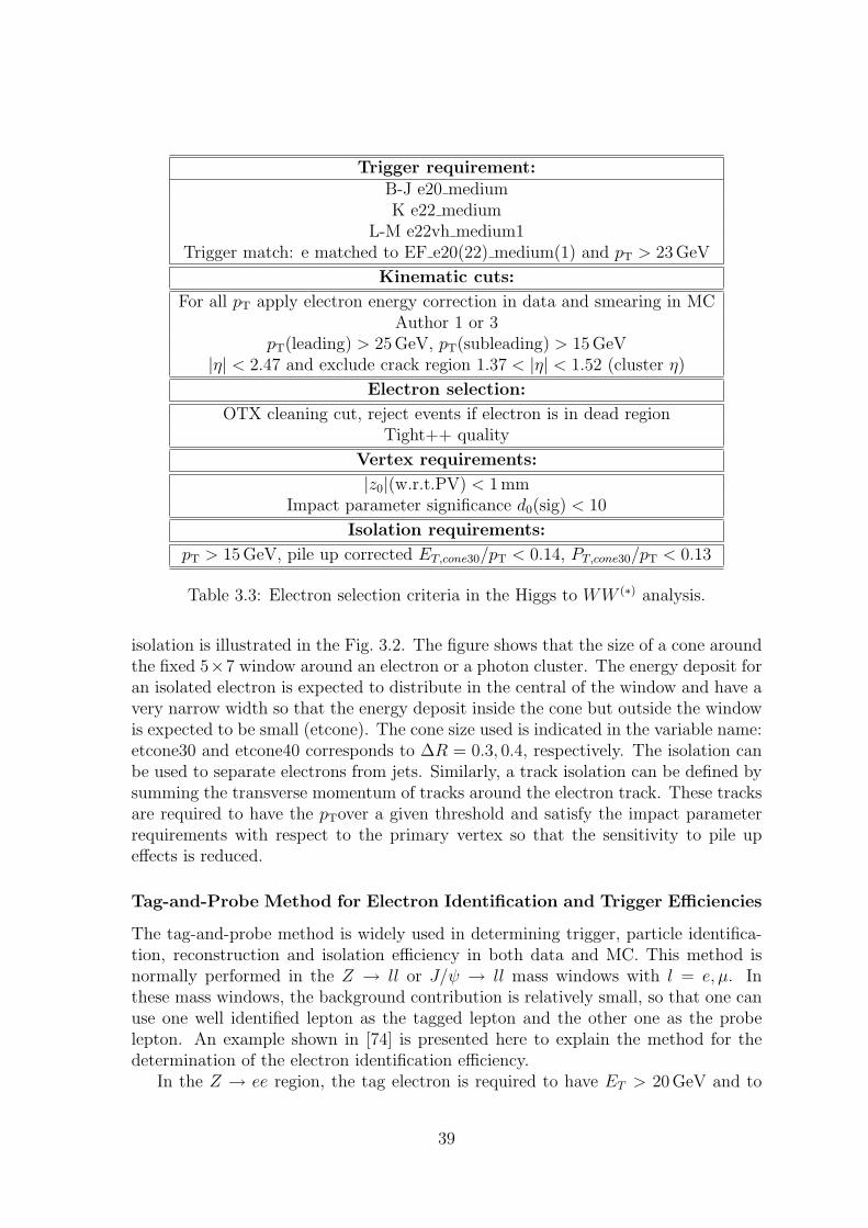
In the Higgs to WW (∗) analysis, the electron selection follows the recommendationof the egamma group. Electrons are required as prompt and isolated. The followingselection criteria are applied as shown in Tab. 3.3.
In the 2011 data analysis the period dependent trigger requirements EF e20 medium,
37
Kinematic variables: eT > 5 GeV; |η| < 2.47
Calorimeter based cuts:
Hadronic leakageRatio e237/e277
Shower width in 2nd samplingTotal width in 1st sampling
Cut on (Emax − Emax2)/(Emax + Emax2) in the 1st sampling
Cuts on track quality:
Pixel hits, SCT hitsB-Layer hits
Outliers for B-layer, Pix, SCT, TRT tracksTRT hits and ratio with outliers
Transverse impact parameter <1 mmEcalo/Etrack cuts
Track cluster match
Table 3.2: Menu of the tight++ electron selection, cut values not shown here areη − φ or η − pT dependent. e237 means the energy deposition in 3 × 7 cells area inlayer 2. e277 means the energy deposition in 7 × 7 cells area in layer 2. Emax is themaximum energy deposition of a cell in the cluster in the 1st sampling and Emax2 isthe second largest energy deposition.
EF e22 medium and EF e22vh medium1 are used to cope with the increasing lumi-nosity and pile up. The periods for data are defined by different luminosity in datataking. The numbers after EF e in the names represent the nominal pT thresholdvalues for these triggers. The suffix medium and medium1 indicate the tightness inthe electron identification and vh means that the trigger has both η dependent pT
threshold and hadronic leakage cut at level 1. An electron trigger is required for theee channel and either an electron or a muon trigger is required for the eµ channel.To suppress QCD contamination, the lepton transverse momentum has to be abovea threshold: 25 GeV for the leading lepton and for 15GeV for the subleading lepton.The higher lepton pT threshold helps in rejecting more fake or non-prompt electronsbut it also reduces the selection efficiency for low Higgs mass points below about130 GeV. The η cut is made to avoid the crack region in the EM calorimeter. In the2011 data taking, part of the LAr Front-End-Board opto-transmitter plug-ins (OTX)were dead and could not be replaced immediately so that events which have electronsin these regions are rejected. The tight++ identified electrons are selected. In suchtight++ menu a series of optimised cuts are made to distinguish a genuine electronfrom a fake one by comparing the shower shape, track quality and hadronic leak-age. Also the associated track of an electron candidate should have a primary vertexwhich has small impact parameters and their significance. The impact parametersignificance is defined as the parameter such as d0 and z0 over their errors. To furtherisolate the electrons, a set of cluster and track isolation cuts are applied. The cluster
38
Trigger requirement:B-J e20 mediumK e22 medium
L-M e22vh medium1Trigger match: e matched to EF e20(22) medium(1) and pT > 23GeV
Kinematic cuts:
For all pT apply electron energy correction in data and smearing in MCAuthor 1 or 3
pT(leading) > 25GeV, pT(subleading) > 15GeV|η| < 2.47 and exclude crack region 1.37 < |η| < 1.52 (cluster η)
Electron selection:
OTX cleaning cut, reject events if electron is in dead regionTight++ quality
Vertex requirements:
|z0|(w.r.t.PV) < 1 mmImpact parameter significance d0(sig) < 10
Isolation requirements:
pT > 15GeV, pile up corrected ET,cone30/pT < 0.14, PT,cone30/pT < 0.13
Table 3.3: Electron selection criteria in the Higgs to WW (∗) analysis.
isolation is illustrated in the Fig. 3.2. The figure shows that the size of a cone aroundthe fixed 5×7 window around an electron or a photon cluster. The energy deposit foran isolated electron is expected to distribute in the central of the window and have avery narrow width so that the energy deposit inside the cone but outside the windowis expected to be small (etcone). The cone size used is indicated in the variable name:etcone30 and etcone40 corresponds to ∆R = 0.3, 0.4, respectively. The isolation canbe used to separate electrons from jets. Similarly, a track isolation can be defined bysumming the transverse momentum of tracks around the electron track. These tracksare required to have the pTover a given threshold and satisfy the impact parameterrequirements with respect to the primary vertex so that the sensitivity to pile upeffects is reduced.
Tag-and-Probe Method for Electron Identification and Trigger Efficiencies
The tag-and-probe method is widely used in determining trigger, particle identifica-tion, reconstruction and isolation efficiency in both data and MC. This method isnormally performed in the Z → ll or J/ψ → ll mass windows with l = e, µ. Inthese mass windows, the background contribution is relatively small, so that one canuse one well identified lepton as the tagged lepton and the other one as the probelepton. An example shown in [74] is presented here to explain the method for thedetermination of the electron identification efficiency.
In the Z → ee region, the tag electron is required to have ET > 20GeV and to
39
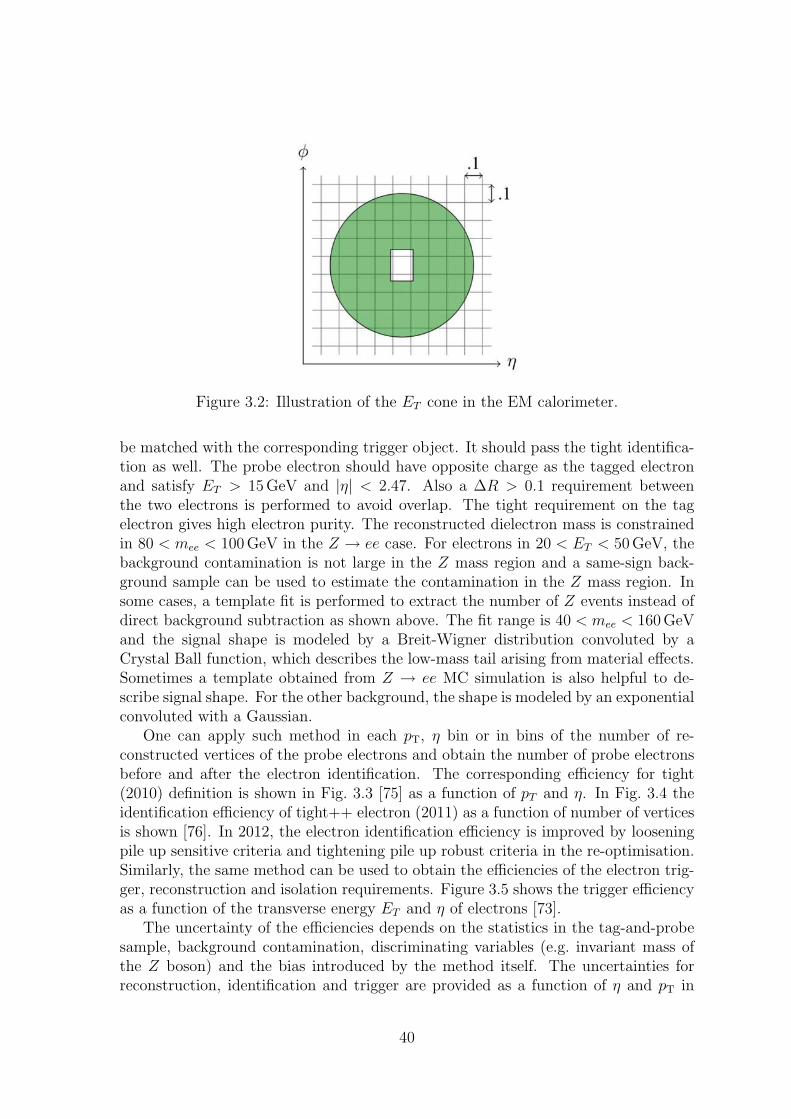
Figure 3.2: Illustration of the ET cone in the EM calorimeter.
be matched with the corresponding trigger object. It should pass the tight identifica-tion as well. The probe electron should have opposite charge as the tagged electronand satisfy ET > 15GeV and |η| < 2.47. Also a ∆R > 0.1 requirement betweenthe two electrons is performed to avoid overlap. The tight requirement on the tagelectron gives high electron purity. The reconstructed dielectron mass is constrainedin 80 < mee < 100 GeV in the Z → ee case. For electrons in 20 < ET < 50GeV, thebackground contamination is not large in the Z mass region and a same-sign back-ground sample can be used to estimate the contamination in the Z mass region. Insome cases, a template fit is performed to extract the number of Z events instead ofdirect background subtraction as shown above. The fit range is 40 < mee < 160 GeVand the signal shape is modeled by a Breit-Wigner distribution convoluted by aCrystal Ball function, which describes the low-mass tail arising from material effects.Sometimes a template obtained from Z → ee MC simulation is also helpful to de-scribe signal shape. For the other background, the shape is modeled by an exponentialconvoluted with a Gaussian.
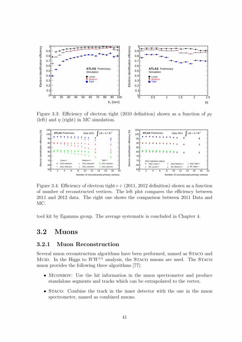
One can apply such method in each pT, η bin or in bins of the number of re-constructed vertices of the probe electrons and obtain the number of probe electronsbefore and after the electron identification. The corresponding efficiency for tight(2010) definition is shown in Fig. 3.3 [75] as a function of pT and η. In Fig. 3.4 theidentification efficiency of tight++ electron (2011) as a function of number of verticesis shown [76]. In 2012, the electron identification efficiency is improved by looseningpile up sensitive criteria and tightening pile up robust criteria in the re-optimisation.Similarly, the same method can be used to obtain the efficiencies of the electron trig-ger, reconstruction and isolation requirements. Figure 3.5 shows the trigger efficiencyas a function of the transverse energy ET and η of electrons [73].
The uncertainty of the efficiencies depends on the statistics in the tag-and-probesample, background contamination, discriminating variables (e.g. invariant mass ofthe Z boson) and the bias introduced by the method itself. The uncertainties forreconstruction, identification and trigger are provided as a function of η and pT in
40
[GeV]TE
10 20 30 40 50 60 70 80 90 100
Ele
ctro
n id
entif
icat
ion
effic
ienc
y
0
0.1
0.2
0.3
0.4
0.5
0.6
0.7
0.8
0.9
1
LooseMediumTight
ATLAS PreliminarySimulation
|η|
0 0.5 1 1.5 2 2.5
Ele
ctro
n id
entif
icat
ion
effic
ienc
y
0
0.1
0.2
0.3
0.4
0.5
0.6
0.7
0.8
0.9
1
LooseMediumTight
ATLAS PreliminarySimulation
Figure 3.3: Efficiency of electron tight (2010 definition) shown as a function of pT
(left) and η (right) in MC simulation.
Number of reconstructed primary vertices
0 2 4 6 8 10 12 14 16 18 20
Ele
ctro
n id
entif
icat
ion
effic
ienc
y [%
]
60
65
70
75
80
85
90
95
100
105ATLAS Preliminary -1
4.7 fb≈ Ldt ∫Data 2011
Loose++
2012 selection
2011 selection
Medium++
2012 selection
2011 selection
Tight++
2012 selection
2011 selection
Number of reconstructed primary vertices
0 2 4 6 8 10 12 14 16 18 20
Ele
ctro
n id
entif
icat
ion
effic
ienc
y [%
]
60
65
70
75
80
85
90
95
100
105ATLAS Preliminary -1
4.7 fb≈ Ldt ∫Data 2011
2012 selection criteriaData Loose++
MC Loose++
Data Medium++
MC Medium++
Data Tight++
MC Tight++
Figure 3.4: Efficiency of electron tight++ (2011, 2012 definition) shown as a functionof number of reconstructed vertices. The left plot compares the efficiency between2011 and 2012 data. The right one shows the comparison between 2011 Data andMC.
tool kit by Egamma group. The average systematic is concluded in Chapter 4.
3.2 Muons
3.2.1 Muon Reconstruction
Several muon reconstruction algorithms have been performed, named as Staco andMuid. In the Higgs to WW (∗) analysis, the Staco muons are used. The Staco
muon provides the following three algorithms [77]:
• Muonboy: Use the hit information in the muon spectrometer and producestandalone segments and tracks which can be extrapolated to the vertex.
• Staco: Combine the track in the inner detector with the one in the muonspectrometer, named as combined muons.
41
(GeV)Telectron E
10 15 20 25 30 35 40 45 50 55 60
Trig
ger
eff.
0
0.2
0.4
0.6
0.8
1
ATLAS Preliminary-1
Ldt=206 pb∫Data 2011
e20_medium trigger
>14 GeV)T
L1 (E
>19 GeV)T
L2 (E
>20 GeV)T
EF (E
ηelectron
-2 -1 0 1 2
Trig
ger
eff.
0.8
0.82
0.84
0.86
0.88
0.9
0.92
0.94
0.96
0.98
1
1.02
ATLAS Preliminary-1
Ldt=206 pb∫Data 2011
e20_medium trigger
>14 GeV)T
L1 (E
>19 GeV)T
L2 (E
>20 GeV)T
EF (E
Figure 3.5: Trigger efficiency of electron e20 medium shown as a function of thetransverse energy ET (left) and η (right)
• Mutag: Combine the Muonboy segment not included in the Staco algorithmwith an inner detector track.
The Staco algorithm loops in two muon track containers, MS and ID, comparesthe parameter vectors and their covariance matrices in the ID and MS to find theminimum χ2 and to match one ID track and one MS track when the χ2 is withina given cut value. Through this procedure the combined muons are obtained in theregion |η| < 2.5.
3.2.2 Muons Selection in H → WW (∗) Analysis
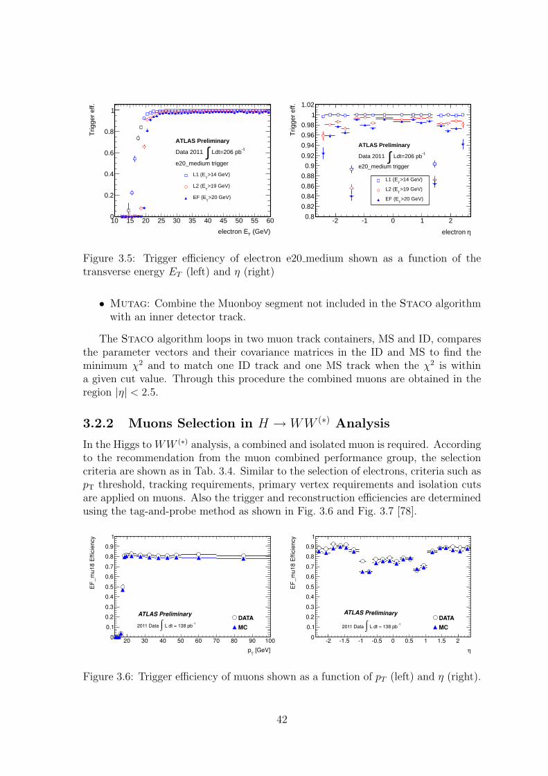
In the Higgs to WW (∗) analysis, a combined and isolated muon is required. Accordingto the recommendation from the muon combined performance group, the selectioncriteria are shown as in Tab. 3.4. Similar to the selection of electrons, criteria such aspT threshold, tracking requirements, primary vertex requirements and isolation cutsare applied on muons. Also the trigger and reconstruction efficiencies are determinedusing the tag-and-probe method as shown in Fig. 3.6 and Fig. 3.7 [78].
[GeV]T
p
20 30 40 50 60 70 80 90 100
EF
_m
u18 E
ffic
iency
0
0.1
0.2
0.3
0.4
0.5
0.6
0.7
0.8
0.9
1
DATA
MC
ATLAS Preliminary
-1 L dt = 138 pb∫2011 Data
η
-2 -1.5 -1 -0.5 0 0.5 1 1.5 2
EF
_m
u18 E
ffic
iency
0
0.1
0.2
0.3
0.4
0.5
0.6
0.7
0.8
0.9
1
DATA
MC
ATLAS Preliminary
-1 L dt = 138 pb∫2011 Data
Figure 3.6: Trigger efficiency of muons shown as a function of pT (left) and η (right).
42
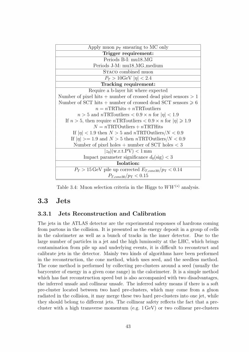
Apply muon pT smearing to MC onlyTrigger requirement:Periods B-I: mu18 MG
Periods J-M: mu18 MG mediumStaco combined muonPT > 10GeV |η| < 2.4
Tracking requirement:Require a b-layer hit where expected
Number of pixel hits + number of crossed dead pixel sensors > 1Number of SCT hits + number of crossed dead SCT sensors > 6
n = nTRThits + nTRToutliersn > 5 and nTRToutliers < 0.9 × n for |η| < 1.9
If n > 5, then require nTRToutliers < 0.9 × n for |η| > 1.9N = nTRTOutliers + nTRTHits
If |η| < 1.9 then N > 5 and nTRTOutliers/N < 0.9If |η| >= 1.9 and N > 5 then nTRTOutliers/N < 0.9Number of pixel holes + number of SCT holes < 3
|z0|(w.r.t.PV) < 1 mmImpact parameter significance d0(sig) < 3
Isolation:PT > 15GeV pile up corrected ET,cone30/pT < 0.14
PT,cone30/pT < 0.15
Table 3.4: Muon selection criteria in the Higgs to WW (∗) analysis.
3.3 Jets
3.3.1 Jets Reconstruction and Calibration
The jets in the ATLAS detector are the experimental responses of hardrons comingfrom partons in the collision. It is presented as the energy deposit in a group of cellsin the calorimeter as well as a bunch of tracks in the inner detector. Due to thelarge number of particles in a jet and the high luminosity at the LHC, which bringscontamination from pile up and underlying events, it is difficult to reconstruct andcalibrate jets in the detector. Mainly two kinds of algorithms have been performedin the reconstruction, the cone method, which uses seed, and the seedless method.The cone method is performed by collecting pre-clusters around a seed (usually thebarycenter of energy in a given cone range) in the calorimeter. It is a simple methodwhich has fast reconstruction speed but is also accompanied with two disadvantages,the inferred unsafe and collinear unsafe. The inferred safety means if there is a softpre-cluster located between two hard pre-clusters, which may come from a gluonradiated in the collision, it may merge these two hard pre-clusters into one jet, whilethey should belong to different jets. The collinear safety reflects the fact that a pre-cluster with a high transverse momentum (e.g. 1 GeV) or two collinear pre-clusters
43
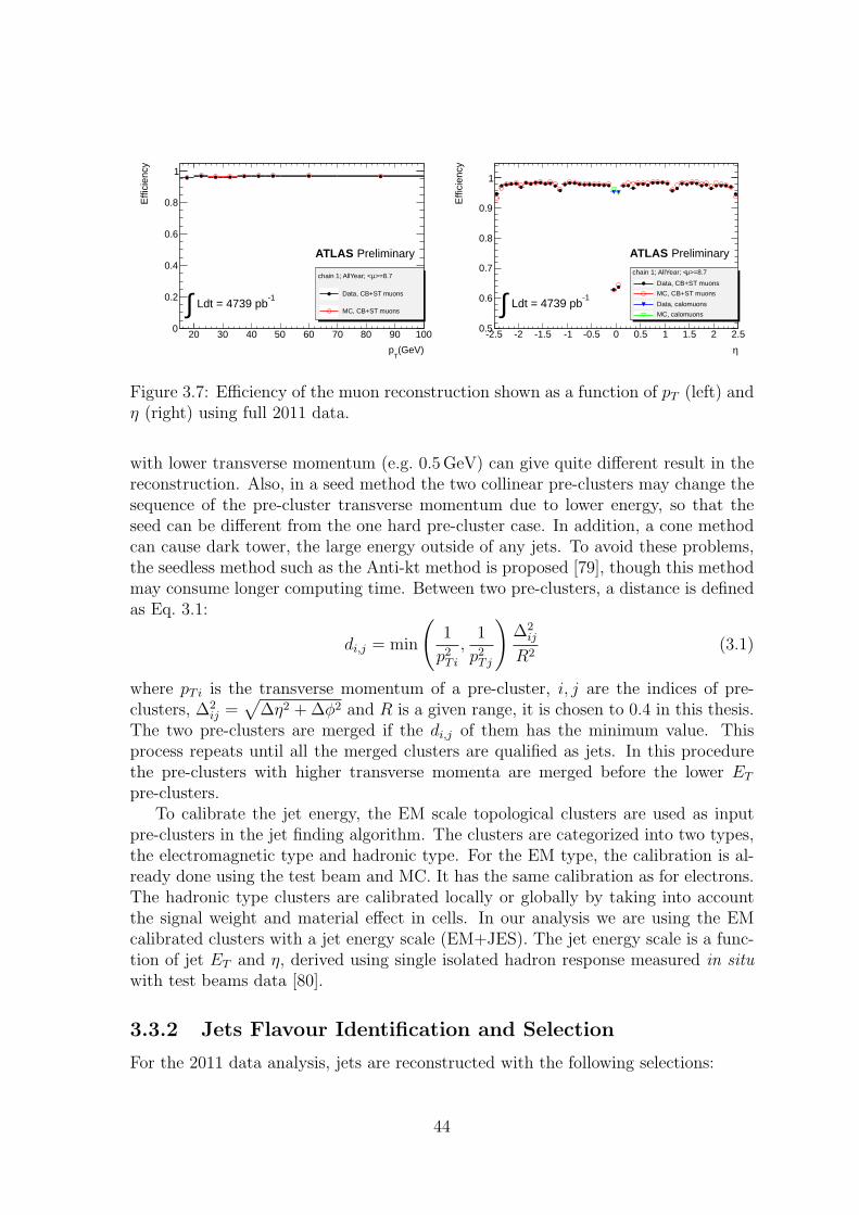
(GeV)T
p
20 30 40 50 60 70 80 90 100
Effi
cien
cy
0
0.2
0.4
0.6
0.8
1
>=8.7µchain 1; AllYear; <
Data, CB+ST muons
MC, CB+ST muons
-1 Ldt = 4739 pb∫
ATLAS Preliminary
η
-2.5 -2 -1.5 -1 -0.5 0 0.5 1 1.5 2 2.5
Effi
cien
cy
0.5
0.6
0.7
0.8
0.9
1
>=8.7µchain 1; AllYear; <
Data, CB+ST muons
MC, CB+ST muons
Data, calomuons
MC, calomuons
-1 Ldt = 4739 pb∫
ATLAS Preliminary
Figure 3.7: Efficiency of the muon reconstruction shown as a function of pT (left) andη (right) using full 2011 data.
with lower transverse momentum (e.g. 0.5 GeV) can give quite different result in thereconstruction. Also, in a seed method the two collinear pre-clusters may change thesequence of the pre-cluster transverse momentum due to lower energy, so that theseed can be different from the one hard pre-cluster case. In addition, a cone methodcan cause dark tower, the large energy outside of any jets. To avoid these problems,the seedless method such as the Anti-kt method is proposed [79], though this methodmay consume longer computing time. Between two pre-clusters, a distance is definedas Eq. 3.1:
di,j = min
(
1
p2T i
,1
p2Tj
)
∆2ij
R2(3.1)
where pT i is the transverse momentum of a pre-cluster, i, j are the indices of pre-clusters, ∆2
ij =√
∆η2 + ∆φ2 and R is a given range, it is chosen to 0.4 in this thesis.The two pre-clusters are merged if the di,j of them has the minimum value. Thisprocess repeats until all the merged clusters are qualified as jets. In this procedurethe pre-clusters with higher transverse momenta are merged before the lower ET
pre-clusters.To calibrate the jet energy, the EM scale topological clusters are used as input
pre-clusters in the jet finding algorithm. The clusters are categorized into two types,the electromagnetic type and hadronic type. For the EM type, the calibration is al-ready done using the test beam and MC. It has the same calibration as for electrons.The hadronic type clusters are calibrated locally or globally by taking into accountthe signal weight and material effect in cells. In our analysis we are using the EMcalibrated clusters with a jet energy scale (EM+JES). The jet energy scale is a func-tion of jet ET and η, derived using single isolated hadron response measured in situ
with test beams data [80].
3.3.2 Jets Flavour Identification and Selection
For the 2011 data analysis, jets are reconstructed with the following selections:
44
• The jets are in the region |η| < 4.5 with ET > 25GeV.
• Overlap removal is performed between jets and any selected electrons.
• To identify jets coming from b quarks, b-tagging is performed. The jet b-flavourweight is calculated by the combined neural network method, which exploitsthe impact parameter significance and the topology of b and c hadron decays.The b-jets should have weight larger than −1.25 corresponding to a workingpoint with 80% efficiency [81]. The b-tagging is only performed in |η| < 2.5 andET > 20GeV.
• A cut on the jet vertex fraction (JVF) JVF> 0.75 is also applied for jets in|η| < 2.1. The JVF is the fraction of the summed pT of tracks which belong tojets pointing back to the primary vertex. This is needed to reduce contributionsfrom pile up effects.
• In the high pile up condition a significant excess has been observed in 2.5 ≤|η| ≤ 3.5 due to the in- and out-of-time pile up (pile up effect in the sameor successive bunch crossing) as well as worse granularity and resolution of thecalorimeter subdetectors in the transition region between the EMEC and FCALdetectors. Finally all the jets in the range 2.5 ≤ |η| ≤ 3.5 are required to havea higher ET threshold at 30 GeV.
3.4 Transverse Missing Energy
The transverse missing energy EmissT is reconstructed by summing energy over all of
the cells in the calorimeter, taking into account the muon pT , the energy loss in thecryostat, and cells not associated with any objects [82]:
Emissx(y) = Emiss,e
x(y) + Emiss,γx(y) + Emiss,τ
x(y) + Emiss,jetsx(y)
+Emiss,soft jetsx(y) + Emiss,CellOut
x(y) + Emiss,µx(y) , (3.2)
The EmissT used in this analysis, which is called MET RefFinal, is calibrated by a
refined calibration: apply different weights to cells that belong to different recon-structed objects such as electrons and jets [83]. The Emiss
T is an important componentin reconstructing Higgs transverse mass, see Eq. 4.6 in Chapter 4. As there are miss-ing neutrinos from decays of the WW (∗) final state, the Emiss
T gives a measurementof the transverse momentum of neutrinos and balances the visible transverse energyfrom leptons and jets. However, the pile up effect, underlying events, resolution ofsoft hardronic candidates or the high pT candidates in the dead region, can cause theimbalance. The imbalance may result in longer Emiss
T tail for the processes which haveno missing energy, such as the Drell-Yan process. The tail can contribute to the Higgssignal region especially in the high pile up condition. To make further suppressionon Drell-Yan and QCD events, the variable actually used in this thesis is defined as
45
EmissT,rel:
EmissT,rel =
{
EmissT if ∆φ ≥ π/2
EmissT × sin ∆φ if ∆φ ≤ π/2
(3.3)
where ∆φ is the absolute difference in the azimuthal angle between the EmissT vector
and the closest lepton or jet in the transverse plane.
3.5 Luminosity Determination
The luminosity in the ATLAS detector is measured using LUCID and BCM as de-scribed in Chapter 2. The integrated luminosity may be defined alternatively as:
L =µvisnbfr
σvis
(3.4)
where µvis is the average number of visible inelastic interactions per bunch crossing(BC) which can be calibrated by the van der Meer (vdM) scan [84], nb and fr arethe number of bunches cross at the interaction point and the revolution frequency inthe collider operation, respectively and σvis = ǫσinel represents the inelastic interac-tion cross section multiplied with the efficiency of the measurement. Therefore theluminosity L is determined by the value of µvis, which is obtained from counting thenumber of the measured inelastic events N and the number of bunch crossings NBC.When µvis ≪ 1 the µvis is simply N/NBC, otherwise it follows a Poisson distribution:
PEvent,OR(µORvis ) =
NOR
NBC
= 1 − e−µORvis (3.5)
µORvis = − ln
(
1 − NOR
NBC
)
. (3.6)
This shows the relation between the average inelastic interaction in every bunchcrossing and the number of observed events on either side of LUCID over the numberof bunch crossings in a period. Also, one can get the probability that observing eventson both sides of LUCID simultaneously, but it is more complicated. In the 2011 datataking, the peak µvis reached a relatively high value up to 24 and in 2012, this numbercan be as high as 40 (Fig. 3.8). The systematic uncertainty for the 2011 luminositymeasurement is 3.9% [104] 1. This number is 3.6% for the 2012 8 TeV measurement.
1The uncertainty is now improved to 1.8% [105].
46
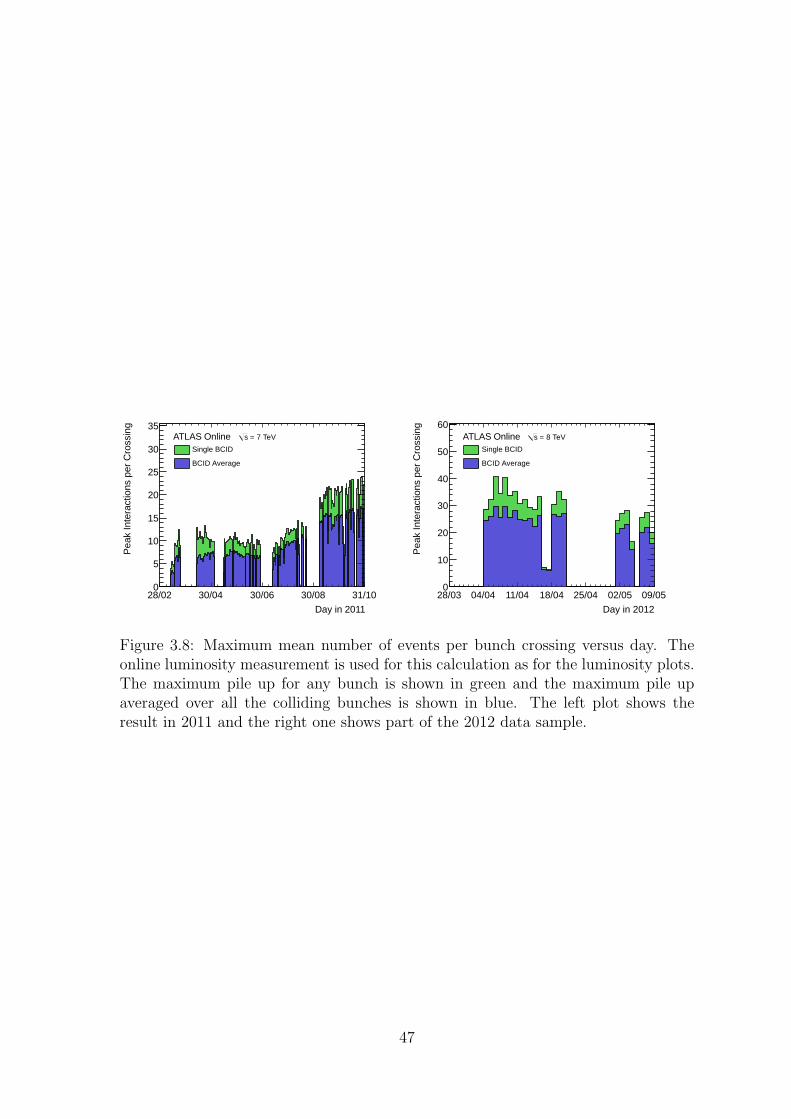
Day in 2011
28/02 30/04 30/06 30/08 31/10
Pea
k In
tera
ctio
ns p
er C
ross
ing
0
5
10
15
20
25
30
35 = 7 TeVs ATLAS Online
Single BCID
BCID Average
Day in 2012
28/03 04/04 11/04 18/04 25/04 02/05 09/05
Pea
k In
tera
ctio
ns p
er C
ross
ing
0
10
20
30
40
50
60 = 8 TeVs ATLAS Online
Single BCID
BCID Average
Figure 3.8: Maximum mean number of events per bunch crossing versus day. Theonline luminosity measurement is used for this calculation as for the luminosity plots.The maximum pile up for any bunch is shown in green and the maximum pile upaveraged over all the colliding bunches is shown in blue. The left plot shows theresult in 2011 and the right one shows part of the 2012 data sample.
47
Chapter 4
Event Selection in Higgs toWW (∗) to lνlν Analysis
In this study, the Standard Model Higgs boson search is performed in the WW (∗)
diboson channel, which has the largest decay branching fraction over all the decaymodes in the intermediate Higgs mass region (135 < mH < 240 GeV) and has compa-rable sensitivity in the low Higgs mass region (∼ 130 GeV) as the diphoton channel.Both of the W bosons are required to decay leptonically. In each event two promptand isolated leptons are selected to suppress QCD background contamination in ppcollisions. The dilepton final states have three lepton flavour combinations in the finalstate: ee, µµ and eµ. The electrons and muons arise from both the direct decay inW → eν, W → µν and a cascade decay W → τν; τ → eν or µν. The neutrinos in thedecay cannot be detected in the detector, however, the missing neutrinos contributeto the missing energy in the transverse plane. Thus, the transverse mass of the Higgsboson is reconstructed instead of a full invariant mass. The two leptons are requiredto have opposite electric charges due to the neutral Higgs boson.
In addition to charged leptons, there may be jets in the final state. Depending onthe number of jets reconstructed in the event, the background contribution can bevery different. For this reason, events are categorized into 0-jet, 1-jet, more than 2 jets(named as 2-jets hereafter) bins. In the 0-jet bin, the Standard ModelWW continuumrepresents the dominant irreducible background to the signal gg → H → WW (∗),while other background events such as top events can be rejected efficiently with a jetveto requirement. In the 2-jets bin, the vector boson fusion (VBF) process with twoforward going jets is expected to appear. Here, b-tagged jets are used to suppress thedominant top background contribution. Hence, the three flavour combinations andthree jet bins result in nine sub-channels for the Higgs search in the WW (∗) → lνlνchannel.
The search for Higgs boson in a SM-like model with a fourth generation is alsoperformed with the same data analysis. The search sensitivity in the 4-generationmodel is higher than in 3-generation SM because of the larger production cross section,see Chapter 6. All analyses below are performed for the SM case unless explicitlystated otherwise.
The criteria to select leptons, jets and missing transverse energy have already been
48
introduced in Chapter 3. The data and MC samples used in this analysis are presentedin Sections 4.1 and 4.2, respectively. Trigger requirement and event selection cutflows for analyses in 0-, 1- and 2-jets are described in details in Sections 4.3 and4.4. The systematic uncertainties are listed in Section 4.5. Some of the backgroundsare estimated using data-driven methods while others are based the MC predictionswhich are checked with data. The methods to estimate backgrounds will be coveredin Chapter 5.
4.1 Data Sample
The analysis presented here uses the full data sample of 2011 taken by ATLAS at7 TeV. The data sample corresponds to an integrated luminosity of 4.7 fb−1. The datais categorized into period and trigger in the data taking (egamma and muon streams).Different time periods can have different luminosity values, increasing with time. Thesingle muon trigger requires events to have at least one muon with pT > 18GeV. Thesingle electron trigger sets the threshold at 20 or 22 GeV depending on the period, tocope with the increasing event rate. Events with both high pT electrons and muons canbe redundant, so that duplicate removal is performed during the analysis. Each eventshould have a primary vertex with at least three associated tracks of pT > 400 MeVto suppress non-collision background contributions. Quality cuts are also applied toreject events which have fake jets in the region where the detector is not functioningproperly.
4.2 Monte Carlo Samples and Simulations
The Monte Carlo samples for different background processes are produced with vari-ous MC generators, which are listed in Tab. 4.1 together with the corresponding crosssection values. The Higgs signal is generated by POWHEG [85, 86] for ggF and V BFand Pythia [87] for WH and ZH. The cross section and branching ratio values as afunction of the Higgs mass are listed in Tab. 4.2 [88] and compared with the numbersof CERN Yellow Report 1.
Among all the background samples, the W → lν, inclusive Z/γ∗ → ll and Wγ aregenerated by ALPGEN [89], which describes well parton multiplicity distributions.The other backgrounds except gg → WW , bb, single top Wt, t channel are generatedby MC@NLO [90], which provides next-to-leading-order (NLO) calculation. The useof leading-order (LO) AcerMC [91] in single top samples is due to the discrepan-cies in the comparison between MC@NLO and other generators in the b-jet rapiditydistribution.
As the POWHEG and MC@NLO only described the pT distribution of Higgs atleading-order and the pT distribution is sensitive to lepton pT and jet bin migration,it is necessary to reweight Higgs pT distribution to NLO with large log resummationat NNLL (Next-to-Next-to-Leading-Log) [92].
In addition, the ALPGEN event generator uses Parton Distribution Functions(PDFs) CTEQ6L1 [93], a LO PDF set such that the description on lepton kinematics
49
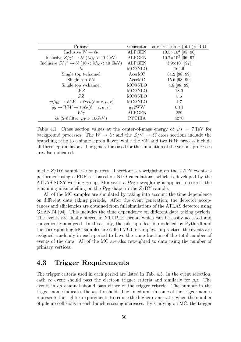
Process Generator cross-section σ (pb) (× BR)
Inclusive W → ℓν ALPGEN 10.5×10³ [95, 96]Inclusive Z/γ∗ → ℓℓ (Mℓℓ > 40 GeV) ALPGEN 10.7×10² [96, 97]
Inclusive Z/γ∗ → ℓℓ (10 < Mℓℓ < 40 GeV) ALPGEN 3.9×10³ [97]tt MC@NLO 164.6
Single top t-channel AcerMC 64.2 [98, 99]Single top Wt AcerMC 15.6 [98, 99]
Single top s-channel MC@NLO 4.6 [98, 99]WZ MC@NLO 18.0ZZ MC@NLO 5.6
qq/qg → WW → ℓνℓν(ℓ = e, µ, τ) MC@NLO 4.7gg → WW → ℓνℓν(ℓ = e, µ, τ) gg2WW 0.14
Wγ ALPGEN 289bb (2-ℓ filter, pT > 10GeV ) PYTHIA 4270
Table 4.1: Cross section values at the center-of-mass energy of√s = 7 TeV for
background processes. The W → ℓν and the Z/γ∗ → ℓℓ cross sections include thebranching ratio to a single lepton flavor, while the γW and two WW process includeall three lepton flavors. The generators used for the simulation of the various processesare also indicated.
in the Z/DY sample is not perfect. Therefore a reweighting on the Z/DY events isperformed using a PDF set based on NLO calculations, which is developed by theATLAS SUSY working group. Moreover, a PT ll reweighting is applied to correct theremaining mismodelling on the PT ll shape in the Z/DY sample.
All of the MC samples are simulated by taking into account the time dependenceon different data taking periods. After the event generation, the detector accep-tances and efficiencies are obtained from full simulations of the ATLAS detector usingGEANT4 [94]. This includes the time dependence on different data taking periods.The events are finally stored in NTUPLE format which can be easily accessed andconveniently analyzed. In this study, the pile up effect is modelled by Pythia 6 andthe corresponding MC samples are called MC11c samples. In practice, the events areassigned randomly in each period to have the same fraction of the total number ofevents of the data. All of the MC are also reweighted to data using the number ofprimary vertices.
4.3 Trigger Requirements
The trigger criteria used in each period are listed in Tab. 4.3. In the event selection,each ee event should pass the electron trigger criteria and similarly for µµ. Theevents in eµ channel should pass either of the trigger criteria. The number in thetrigger name indicates the pT threshold. The “medium” in some of the trigger namesrepresents the tighter requirements to reduce the higher event rates when the numberof pile up collisions in each bunch crossing increases. By studying on MC, the trigger
50
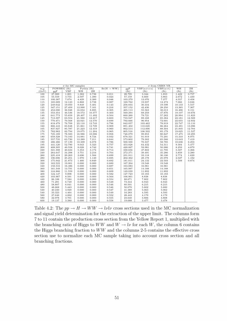
σ for MC samples σ from CERN YRmH POWHEG (fb) Pythia (fb) Br(H → WW) ggF VBF(u+t+s) VBF(u+t) WH ZH
(GeV) ggF VBF WH ZH (fb) (fb) (fb) (fb) (fb)100 27.989 1.801 1.382 0.736 0.011 28.795 3.344 1.853 1.422 0.757105 55.559 3.755 2.597 1.390 0.024 57.159 6.669 3.863 2.672 1.430110 100.387 7.074 4.429 2.389 0.048 103.279 12.076 7.277 4.557 2.458115 165.009 12.123 6.868 3.738 0.087 169.762 19.937 12.472 7.066 3.846120 249.642 19.050 9.849 5.401 0.143 256.834 30.334 19.598 10.133 5.557125 347.151 27.459 12.990 7.161 0.216 357.152 42.436 28.250 13.365 7.367130 452.090 36.948 16.034 8.895 0.305 465.113 55.563 38.013 16.496 9.151135 553.354 46.536 18.572 10.377 0.403 569.294 68.259 47.876 19.107 10.676140 641.773 55.659 20.407 11.492 0.504 660.260 79.721 57.262 20.994 11.823145 713.397 63.554 21.560 12.217 0.603 733.947 89.168 65.384 22.181 12.569150 770.471 70.568 22.021 12.570 0.699 792.666 96.954 72.601 22.655 12.932155 818.479 76.709 22.110 12.743 0.796 842.057 103.462 78.919 22.747 13.110160 866.443 83.848 21.861 12.729 0.909 891.402 110.620 86.264 22.491 13.096165 837.927 85.787 21.223 12.419 0.960 862.514 112.006 88.304 21.845 12.784170 782.962 82.794 19.075 11.204 0.965 805.516 106.502 85.179 19.625 11.527175 725.189 78.583 16.986 10.006 0.958 746.079 99.853 80.847 17.475 10.295180 659.328 73.183 14.881 8.724 0.932 678.321 91.919 75.291 15.310 8.975185 557.735 63.730 12.289 7.211 0.844 573.802 79.302 65.566 12.643 7.419190 486.486 57.139 10.339 6.078 0.786 500.500 70.347 58.785 10.636 6.253195 441.120 52.790 9.043 5.323 0.757 453.828 64.432 54.311 9.304 5.477200 408.305 49.558 8.028 4.742 0.741 420.067 59.981 50.986 8.259 4.879220 321.398 40.624 5.353 3.174 0.714 330.656 47.802 41.795 5.507 3.266240 264.647 34.298 3.751 2.216 0.704 272.271 39.491 35.286 3.859 2.280260 225.418 29.263 2.696 1.584 0.699 231.911 33.118 30.106 2.774 1.629280 196.696 25.251 1.970 1.149 0.695 202.362 28.178 25.978 2.027 1.182300 175.942 21.873 1.466 0.849 0.692 181.011 24.132 22.503 1.508 0.874320 162.522 19.001 0.000 0.000 0.689 167.204 19.548 19.548340 158.516 16.486 0.000 0.000 0.687 163.083 16.961 16.961360 161.349 13.791 0.000 0.000 0.651 165.997 14.188 14.188380 144.866 11.559 0.000 0.000 0.609 149.039 11.892 11.892400 124.147 9.898 0.000 0.000 0.582 127.723 10.183 10.183420 103.967 8.591 0.000 0.000 0.564 106.961 8.838 8.838440 86.188 7.584 0.000 0.000 0.554 88.671 7.802 7.802460 71.291 6.749 0.000 0.000 0.549 73.344 6.943 6.943480 58.807 6.041 0.000 0.000 0.546 60.501 6.215 6.215500 48.668 5.443 0.000 0.000 0.546 50.070 5.602 5.600520 40.230 4.920 0.000 0.000 0.547 41.389 5.063 5.062540 33.323 4.464 0.000 0.000 0.549 34.283 4.595 4.593560 27.646 4.062 0.000 0.000 0.552 28.443 4.179 4.179580 22.978 3.701 0.000 0.000 0.555 23.640 3.806 3.808600 19.137 3.380 0.000 0.000 0.558 19.688 3.477 3.478
Table 4.2: The pp→ H → WW → lνlν cross sections used in the MC normalizationand signal yield determination for the extraction of the upper limit. The columns form7 to 11 contain the production cross section from the Yellow Report 1, multiplied withthe branching ratio of Higgs to WW and W → lν for each W , the column 6 containsthe Higgs branching fraction to WW and the columns 2-5 contains the effective crosssection use to normalize each MC sample taking into account cross section and allbranching fractions.
51
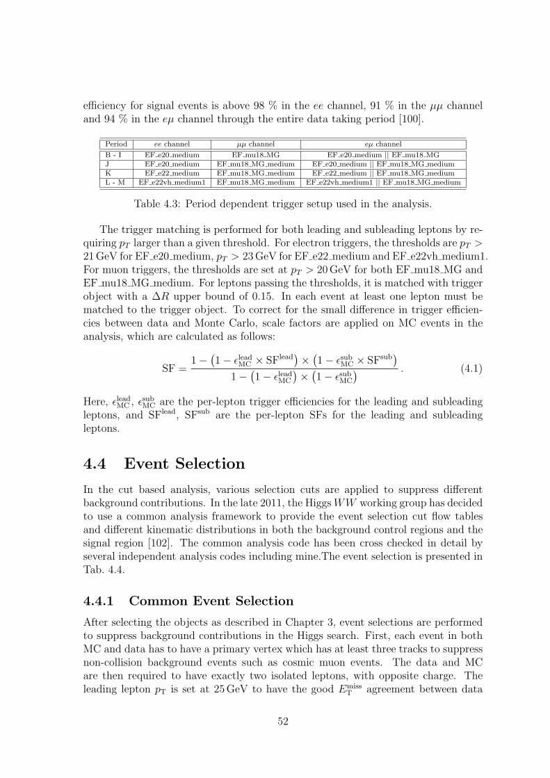
efficiency for signal events is above 98 % in the ee channel, 91 % in the µµ channeland 94 % in the eµ channel through the entire data taking period [100].
Period ee channel µµ channel eµ channel
B - I EF e20 medium EF mu18 MG EF e20 medium || EF mu18 MGJ EF e20 medium EF mu18 MG medium EF e20 medium || EF mu18 MG mediumK EF e22 medium EF mu18 MG medium EF e22 medium || EF mu18 MG mediumL - M EF e22vh medium1 EF mu18 MG medium EF e22vh medium1 || EF mu18 MG medium
Table 4.3: Period dependent trigger setup used in the analysis.
The trigger matching is performed for both leading and subleading leptons by re-quiring pT larger than a given threshold. For electron triggers, the thresholds are pT >21GeV for EF e20 medium, pT > 23GeV for EF e22 medium and EF e22vh medium1.For muon triggers, the thresholds are set at pT > 20GeV for both EF mu18 MG andEF mu18 MG medium. For leptons passing the thresholds, it is matched with triggerobject with a ∆R upper bound of 0.15. In each event at least one lepton must bematched to the trigger object. To correct for the small difference in trigger efficien-cies between data and Monte Carlo, scale factors are applied on MC events in theanalysis, which are calculated as follows:
SF =1 −
(
1 − ǫleadMC × SFlead
)
×(
1 − ǫsubMC × SFsub
)
1 −(
1 − ǫleadMC
)
×(
1 − ǫsubMC
) . (4.1)
Here, ǫleadMC , ǫsub
MC are the per-lepton trigger efficiencies for the leading and subleadingleptons, and SFlead, SFsub are the per-lepton SFs for the leading and subleadingleptons.
4.4 Event Selection
In the cut based analysis, various selection cuts are applied to suppress differentbackground contributions. In the late 2011, the HiggsWW working group has decidedto use a common analysis framework to provide the event selection cut flow tablesand different kinematic distributions in both the background control regions and thesignal region [102]. The common analysis code has been cross checked in detail byseveral independent analysis codes including mine.The event selection is presented inTab. 4.4.
4.4.1 Common Event Selection
After selecting the objects as described in Chapter 3, event selections are performedto suppress background contributions in the Higgs search. First, each event in bothMC and data has to have a primary vertex which has at least three tracks to suppressnon-collision background events such as cosmic muon events. The data and MCare then required to have exactly two isolated leptons, with opposite charge. Theleading lepton pT is set at 25 GeV to have the good Emiss
T agreement between data
52
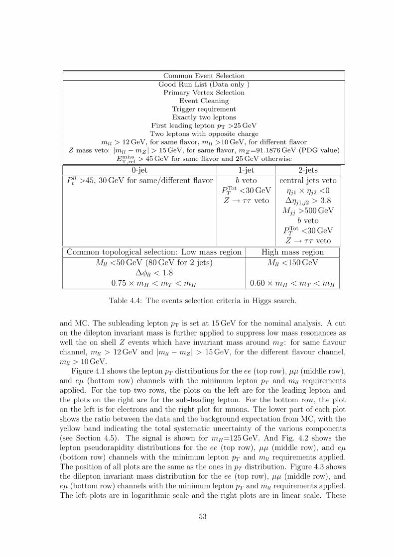
Common Event SelectionGood Run List (Data only )
Primary Vertex SelectionEvent Cleaning
Trigger requirementExactly two leptons
First leading lepton pT >25 GeVTwo leptons with opposite charge
mll > 12 GeV, for same flavor, mll >10 GeV, for different flavorZ mass veto: |mll − mZ | > 15 GeV, for same flavor, mZ=91.1876GeV (PDG value)
EmissT,rel > 45 GeV for same flavor and 25GeV otherwise
0-jet 1-jet 2-jetsP ll
t >45, 30 GeV for same/different flavor b veto central jets vetoPTot
T <30GeV ηj1 × ηj2 <0Z → ττ veto ∆ηj1,j2 > 3.8
Mjj >500 GeVb veto
PTotT <30GeVZ → ττ veto
Common topological selection: Low mass region High mass regionMll <50GeV (80GeV for 2 jets) Mll <150 GeV
∆φll < 1.80.75 ×mH < mT < mH 0.60 ×mH < mT < mH
Table 4.4: The events selection criteria in Higgs search.
and MC. The subleading lepton pT is set at 15 GeV for the nominal analysis. A cuton the dilepton invariant mass is further applied to suppress low mass resonances aswell the on shell Z events which have invariant mass around mZ : for same flavourchannel, mll > 12GeV and |mll − mZ | > 15GeV, for the different flavour channel,mll > 10GeV.
Figure 4.1 shows the lepton pT distributions for the ee (top row), µµ (middle row),and eµ (bottom row) channels with the minimum lepton pT and mll requirementsapplied. For the top two rows, the plots on the left are for the leading lepton andthe plots on the right are for the sub-leading lepton. For the bottom row, the ploton the left is for electrons and the right plot for muons. The lower part of each plotshows the ratio between the data and the background expectation from MC, with theyellow band indicating the total systematic uncertainty of the various components(see Section 4.5). The signal is shown for mH=125 GeV. And Fig. 4.2 shows thelepton pseudorapidity distributions for the ee (top row), µµ (middle row), and eµ(bottom row) channels with the minimum lepton pT and mll requirements applied.The position of all plots are the same as the ones in pT distribution. Figure 4.3 showsthe dilepton invariant mass distribution for the ee (top row), µµ (middle row), andeµ (bottom row) channels with the minimum lepton pT and mll requirements applied.The left plots are in logarithmic scale and the right plots are in linear scale. These
53
plots show good agreement between data and MC.To supress off shell Z/DY events, the relative Emiss
T (EmissT,rel) cut is applied: 45 GeV
for the same flavour channels, 25 GeV for the eµ channel, respectively. The smallercut for the eµ channel is used because the Z/DY events can only come from Z → ττdecays, which is much smaller than the same flavour Z/DY contribution. Figure 4.4shows the Emiss
T,rel distributions of the ee (top row), µµ (middle row), and eµ (bottomrow) channels with the minimum lepton pT and mll requirements applied. The leftplots are in logarithmic scale and right plots in linear scale.
After these common selection cuts, the events are categorized to 0-, 1- and 2-jetbins. The jet multiplicity is shown in Fig. 4.5. Table 4.5 shows the number of dataand expected events in MC after the common selection. Some of the backgrounds arescaled with scale factors derived from data-driven methods, see Chapter 5.
4.4.2 Jet Bin Dependent Selections
In the 0-jet analysis, the transverse momentum of the dilepton system, pllT , is required
to be greater than 45GeV for the eµ channel and 30 GeV for same flavour channelsto suppress more Z/DY events. Also in this region the top contribution is stronglysuppressed. In the 1-jet case, to reject top events, the jet should not be a b-taggedjet.
Another cut concerns pTotT , which is defined as:
pTotT = pl1
T + pl2T + pjets
T + pmissT , (4.2)
and the cut is pTotT < 30GeV.
To suppress the Z → ττ contribution in the eµ channel, a collinear approximationis made. This is based on the assumption that the lepton from the τ decay goes alongthe direction of τ so that if the mass of τ can be neglected the invariant mass of mττ
is approximated as:
mττ =mll√x1x2
, (4.3)
in which x1, x2 are the positive energy fraction carried by the visible particles in theτ decays. They are defined as:
x1 =pl1
x pl2y − pl1
y pl2x
pl2y E
missx − pl2
x Emissy + pl1
x pl2y − pl1
y pl2x
, (4.4)
x2 =pl1
x pl2y − pl1
y pl2x
pl1x E
missy − pl1
y Emissx + pl1
x pl2y − pl1
y pl2x
. (4.5)
The |mττ −mZ | is required to be larger than 25GeV. This cut is applied in 1- and2-jet channels because in the 0-jet channel the two leptons are mostly back to backso that the approximation does not apply.
In the 2-jet analysis, in additon to the b-jet veto, pTotT cuts and Z → ττ veto
cuts mentioned above, the two leading jets are further required to be in differenthemispheres and well separated in pseudorapidity: ∆ηjj ≡ |ηjet1 − ηjet2| > 3.8. Since
54
Eve
nts
/ 5 G
eV
-110
1
10
210
310
410
510
610
710
810 Data stat)⊕ SM (sys
WW γ WZ/ZZ/W
t t Single Top
Z+jets W+jets
H [125 GeV]
ATLAS Internal-1 L dt = 4.7 fb∫ = 7 TeV, s
νeνe→(*)
WW→H
[GeV]T,lead lep
p
20 40 60 80 100 120 140 160 180 2000.70.80.9
11.11.21.3
Eve
nts
/ 5 G
eV
-110
1
10
210
310
410
510
610
710
810 Data stat)⊕ SM (sys
WW γ WZ/ZZ/W
t t Single Top
Z+jets W+jets
H [125 GeV]
ATLAS Internal-1 L dt = 4.7 fb∫ = 7 TeV, s
νeνe→(*)
WW→H
[GeV]T,sublead lep
p
20 40 60 80 100 120 140 160 180 2000.70.80.9
11.11.21.3
Eve
nts
/ 5 G
eV
-110
1
10
210
310
410
510
610
710
810
910 Data stat)⊕ SM (sys
WW γ WZ/ZZ/W
t t Single Top
Z+jets W+jets
H [125 GeV]
ATLAS Internal-1 L dt = 4.7 fb∫ = 7 TeV, s
νµνµ→(*)
WW→H
[GeV]T,lead lep
p
20 40 60 80 100 120 140 160 180 2000.70.80.9
11.11.21.3
Eve
nts
/ 5 G
eV
-110
1
10
210
310
410
510
610
710
810
910 Data stat)⊕ SM (sys
WW γ WZ/ZZ/W
t t Single Top
Z+jets W+jets
H [125 GeV]
ATLAS Internal-1 L dt = 4.7 fb∫ = 7 TeV, s
νµνµ→(*)
WW→H
[GeV]T,sublead lep
p
20 40 60 80 100 120 140 160 180 2000.70.80.9
11.11.21.3
Eve
nts
/ 5 G
eV
-110
1
10
210
310
410
510
Data stat)⊕ SM (sys
WW γ WZ/ZZ/W
t t Single Top
Z+jets W+jets
H [125 GeV]
ATLAS Internal-1 L dt = 4.7 fb∫ = 7 TeV, s
νµνe→(*)
WW→H
[GeV]T,lead lep
p
20 40 60 80 100 120 140 160 180 2000.70.80.9
11.11.21.3
Eve
nts
/ 5 G
eV
-110
1
10
210
310
410
510
610 Data stat)⊕ SM (sys
WW γ WZ/ZZ/W
t t Single Top
Z+jets W+jets
H [125 GeV]
ATLAS Internal-1 L dt = 4.7 fb∫ = 7 TeV, s
νµνe→(*)
WW→H
[GeV]T,sublead lep
p
20 40 60 80 100 120 140 160 180 2000.70.80.9
11.11.21.3
Figure 4.1: Lepton pT distributions for the ee (top row), µµ (middle row), and eµ(bottom row) channels with the minimum lepton pT and mll requirements applied.For the top two rows, the plots on the left are for the leading lepton and the plotson the right are for the sub-leading lepton. For the bottom row, the plot on the leftis for electrons and the right plot for muons. The lower part of each plot shows theratio between the data and the background expectation from MC, with the yellowband indicating the total systematic uncertainty in the normalization (but not theshape) of the various components. The signal is shown for mH = 125 GeV. The finalbin includes the overflow. 55
Eve
nts
/ 0.2
-110
1
10
210
310
410
510
610
710 Data stat)⊕ SM (sys
WW γ WZ/ZZ/W
t t Single Top
Z+jets W+jets
H [125 GeV]
ATLAS Internal-1 L dt = 4.7 fb∫ = 7 TeV, s
νeνe→(*)
WW→H
lead lepη
-3 -2 -1 0 1 2 30.70.80.9
11.11.21.3
Eve
nts
/ 0.2
-110
1
10
210
310
410
510
610
710 Data stat)⊕ SM (sys
WW γ WZ/ZZ/W
t t Single Top
Z+jets W+jets
H [125 GeV]
ATLAS Internal-1 L dt = 4.7 fb∫ = 7 TeV, s
νeνe→(*)
WW→H
sublead lepη
-3 -2 -1 0 1 2 30.70.80.9
11.11.21.3
Eve
nts
/ 0.2
-110
1
10
210
310
410
510
610
710
810 Data stat)⊕ SM (sys
WW γ WZ/ZZ/W
t t Single Top
Z+jets W+jets
H [125 GeV]
ATLAS Internal-1 L dt = 4.7 fb∫ = 7 TeV, s
νµνµ→(*)
WW→H
lead lepη
-3 -2 -1 0 1 2 30.70.80.9
11.11.21.3
Eve
nts
/ 0.2
-110
1
10
210
310
410
510
610
710
810 Data stat)⊕ SM (sys
WW γ WZ/ZZ/W
t t Single Top
Z+jets W+jets
H [125 GeV]
ATLAS Internal-1 L dt = 4.7 fb∫ = 7 TeV, s
νµνµ→(*)
WW→H
sublead lepη
-3 -2 -1 0 1 2 30.70.80.9
11.11.21.3
Eve
nts
/ 0.2
-110
1
10
210
310
410
510 Data stat)⊕ SM (sys
WW γ WZ/ZZ/W
t t Single Top
Z+jets W+jets
H [125 GeV]
ATLAS Internal-1 L dt = 4.7 fb∫ = 7 TeV, s
νµνe→(*)
WW→H
lead lepη
-3 -2 -1 0 1 2 30.70.80.9
11.11.21.3
Eve
nts
/ 0.2
-110
1
10
210
310
410
510 Data stat)⊕ SM (sys
WW γ WZ/ZZ/W
t t Single Top
Z+jets W+jets
H [125 GeV]
ATLAS Internal-1 L dt = 4.7 fb∫ = 7 TeV, s
νµνe→(*)
WW→H
sublead lepη
-3 -2 -1 0 1 2 30.70.80.9
11.11.21.3
Figure 4.2: Lepton pseudorapidity distributions for the ee (top row), µµ (middle row),and eµ (bottom row) channels with the minimum lepton pT and mll requirementsapplied. The layout of the plots is the same as in Fig. 4.1.
56
Eve
nts
/ 10
GeV
-110
1
10
210
310
410
510
610
710
810
910 Data stat)⊕ SM (sys
WW γ WZ/ZZ/W
t t Single Top
Z+jets W+jets
H [125 GeV]
ATLAS Internal-1 L dt = 4.7 fb∫ = 7 TeV, s
νeνe→(*)
WW→H
[GeV]llm
50 100 150 200 2500.70.80.9
11.11.21.3
Eve
nts
/ 10
GeV
100
200
300
400
500
600
700
310× Data stat)⊕ SM (sys
WW γ WZ/ZZ/W
t t Single Top
Z+jets W+jets
H [125 GeV]
ATLAS Internal-1 L dt = 4.7 fb∫ = 7 TeV, s
νeνe→(*)
WW→H
[GeV]llm
50 100 150 200 2500.70.80.9
11.11.21.3
Eve
nts
/ 10
GeV
-110
1
10
210
310
410
510
610
710
810
910 Data stat)⊕ SM (sys
WW γ WZ/ZZ/W
t t Single Top
Z+jets W+jets
H [125 GeV]
ATLAS Internal-1 L dt = 4.7 fb∫ = 7 TeV, s
νµνµ→(*)
WW→H
[GeV]llm
50 100 150 200 2500.70.80.9
11.11.21.3
Eve
nts
/ 10
GeV
200
400
600
800
1000
1200
1400
310× Data stat)⊕ SM (sys
WW γ WZ/ZZ/W
t t Single Top
Z+jets W+jets
H [125 GeV]
ATLAS Internal-1 L dt = 4.7 fb∫ = 7 TeV, s
νµνµ→(*)
WW→H
[GeV]llm
50 100 150 200 2500.70.80.9
11.11.21.3
Eve
nts
/ 10
GeV
-110
1
10
210
310
410
510
610 Data stat)⊕ SM (sys
WW γ WZ/ZZ/W
t t Single Top
Z+jets W+jets
H [125 GeV]
ATLAS Internal-1 L dt = 4.7 fb∫ = 7 TeV, s
νµνe→(*)
WW→H
[GeV]llm
50 100 150 200 2500.70.80.9
11.11.21.3
Eve
nts
/ 10
GeV
1000
2000
3000
4000
5000
Data stat)⊕ SM (sys
WW γ WZ/ZZ/W
t t Single Top
Z+jets W+jets
H [125 GeV]
ATLAS Internal-1 L dt = 4.7 fb∫ = 7 TeV, s
νµνe→(*)
WW→H
[GeV]llm
50 100 150 200 2500.70.80.9
11.11.21.3
Figure 4.3: Dilepton invariant mass distribution for the ee (top row), µµ (middlerow), and eµ (bottom row) channels with the minimum lepton pT and mll require-ments applied. The left plots are in logarithmic scale and the right plots are in linearscale. The lower part of each plot shows the ratio between the data and the back-ground expectation from MC, with the yellow band indicating the total systematicuncertainty in the normalization (but not the shape) of the various components. Thesignal is shown for mH = 125 GeV. The final bin includes the overflow.
57
Eve
nts
/ 4 G
eV
-110
1
10
210
310
410
510
610
710
810 Data stat)⊕ SM (sys
WW γ WZ/ZZ/W
t t Single Top
Z+jets W+jets
H [125 GeV]
ATLAS Internal-1 L dt = 4.7 fb∫ = 7 TeV, s
νeνe→(*)
WW→H
[GeV]T,relmissE
0 20 40 60 80 100 120 140 160 180 2000.70.80.9
11.11.21.3
Eve
nts
/ 4 G
eV
50
100
150
200
250
300
350
400
450310×
Data stat)⊕ SM (sys
WW γ WZ/ZZ/W
t t Single Top
Z+jets W+jets
H [125 GeV]
ATLAS Internal-1 L dt = 4.7 fb∫ = 7 TeV, s
νeνe→(*)
WW→H
[GeV]T,relmissE
0 20 40 60 80 100 120 140 160 180 2000.70.80.9
11.11.21.3
Eve
nts
/ 4 G
eV
-110
1
10
210
310
410
510
610
710
810
910 Data stat)⊕ SM (sys
WW γ WZ/ZZ/W
t t Single Top
Z+jets W+jets
H [125 GeV]
ATLAS Internal-1 L dt = 4.7 fb∫ = 7 TeV, s
νµνµ→(*)
WW→H
[GeV]T,relmissE
0 20 40 60 80 100 120 140 160 180 2000.70.80.9
11.11.21.3
Eve
nts
/ 4 G
eV
100
200
300
400
500
600
700
310× Data stat)⊕ SM (sys
WW γ WZ/ZZ/W
t t Single Top
Z+jets W+jets
H [125 GeV]
ATLAS Internal-1 L dt = 4.7 fb∫ = 7 TeV, s
νµνµ→(*)
WW→H
[GeV]T,relmissE
0 20 40 60 80 100 120 140 160 180 2000.70.80.9
11.11.21.3
Eve
nts
/ 4 G
eV
-110
1
10
210
310
410
510
Data stat)⊕ SM (sys
WW γ WZ/ZZ/W
t t Single Top
Z+jets W+jets
H [125 GeV]
ATLAS Internal-1 L dt = 4.7 fb∫ = 7 TeV, s
νµνe→(*)
WW→H
[GeV]T,relmissE
0 20 40 60 80 100 120 140 160 180 2000.70.80.9
11.11.21.3
Eve
nts
/ 4 G
eV
500
1000
1500
2000
2500
3000
3500
4000
4500 Data stat)⊕ SM (sys
WW γ WZ/ZZ/W
t t Single Top
Z+jets W+jets
H [125 GeV]
ATLAS Internal-1 L dt = 4.7 fb∫ = 7 TeV, s
νµνe→(*)
WW→H
[GeV]T,relmissE
0 20 40 60 80 100 120 140 160 180 2000.70.80.9
11.11.21.3
Figure 4.4: Distribution of EmissT,rel for the ee (top row), µµ (middle row), and eµ
(bottom row) channels with the minimum lepton pT and mll requirements applied.The left plots are in logarithmic scale and right plots in linear scale. The lowerpart of each plot shows the ratio between the data and the background expectationfrom MC, with the yellow band indicating the total systematic uncertainty in thenormalization (but not the shape) of the various components. The signal is shownfor mH = 125 GeV. The final bin includes the overflow.
58
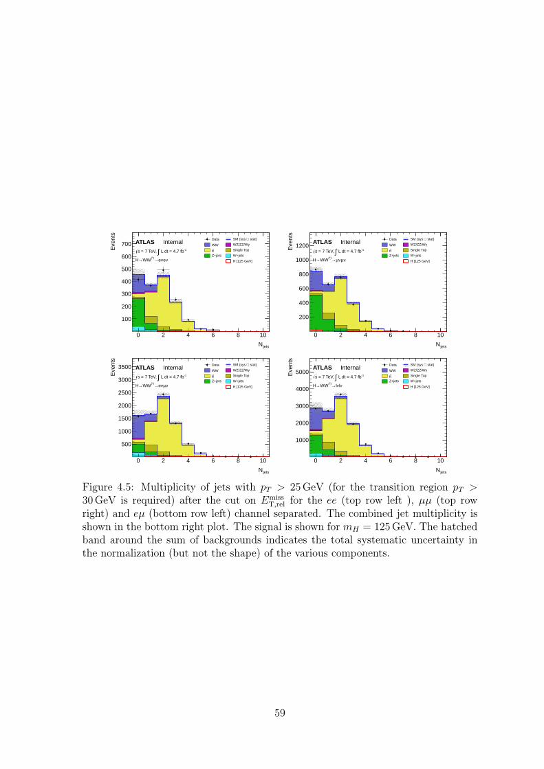
jetsN
0 2 4 6 8 10
Eve
nts
100
200
300
400
500
600
700 Data stat)⊕ SM (sys
WW γ WZ/ZZ/W
t t Single Top
Z+jets W+jets
H [125 GeV]
ATLAS Internal-1 L dt = 4.7 fb∫ = 7 TeV, s
νeνe→(*)WW→H
jetsN
0 2 4 6 8 10
Eve
nts
200
400
600
800
1000
1200 Data stat)⊕ SM (sys
WW γ WZ/ZZ/W
t t Single Top
Z+jets W+jets
H [125 GeV]
ATLAS Internal-1 L dt = 4.7 fb∫ = 7 TeV, s
νµνµ→(*)WW→H
jetsN
0 2 4 6 8 10
Eve
nts
500
1000
1500
2000
2500
3000
3500 Data stat)⊕ SM (sys
WW γ WZ/ZZ/W
t t Single Top
Z+jets W+jets
H [125 GeV]
ATLAS Internal-1 L dt = 4.7 fb∫ = 7 TeV, s
νµνe→(*)WW→H
jetsN
0 2 4 6 8 10
Eve
nts
1000
2000
3000
4000
5000 Data stat)⊕ SM (sys
WW γ WZ/ZZ/W
t t Single Top
Z+jets W+jets
H [125 GeV]
ATLAS Internal-1 L dt = 4.7 fb∫ = 7 TeV, s
νlνl→(*)WW→H
Figure 4.5: Multiplicity of jets with pT > 25GeV (for the transition region pT >30GeV is required) after the cut on Emiss
T,rel for the ee (top row left ), µµ (top rowright) and eµ (bottom row left) channel separated. The combined jet multiplicity isshown in the bottom right plot. The signal is shown for mH = 125 GeV. The hatchedband around the sum of backgrounds indicates the total systematic uncertainty inthe normalization (but not the shape) of the various components.
59
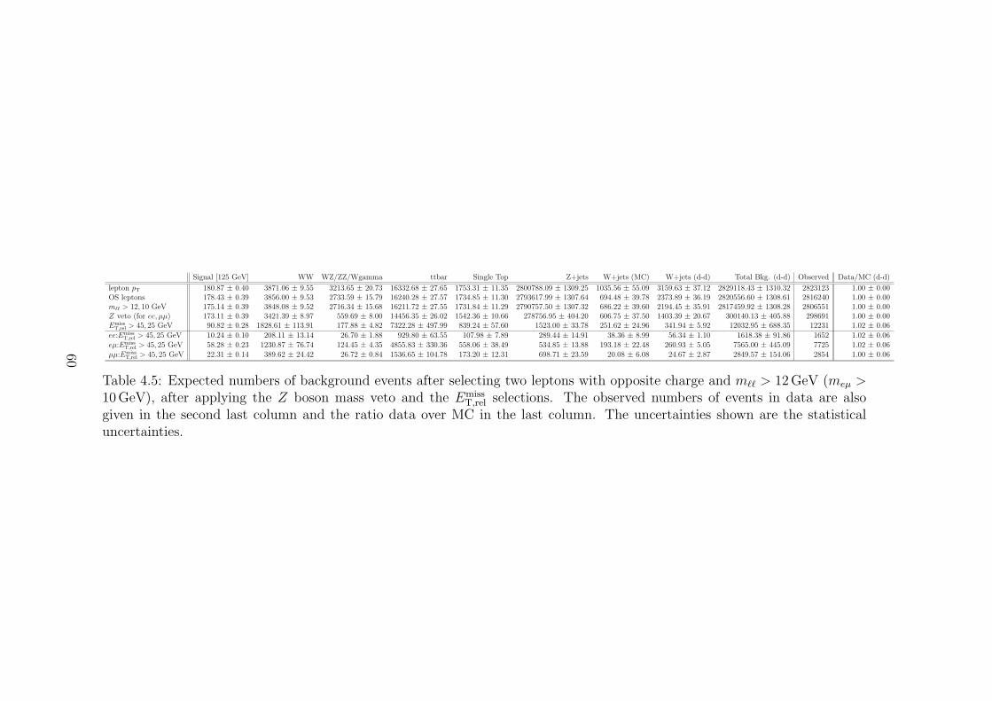
Signal [125 GeV] WW WZ/ZZ/Wgamma ttbar Single Top Z+jets W+jets (MC) W+jets (d-d) Total Bkg. (d-d) Observed Data/MC (d-d)
lepton pT 180.87 ± 0.40 3871.06 ± 9.55 3213.65 ± 20.73 16332.68 ± 27.65 1753.31 ± 11.35 2800788.09 ± 1309.25 1035.56 ± 55.09 3159.63 ± 37.12 2829118.43 ± 1310.32 2823123 1.00 ± 0.00OS leptons 178.43 ± 0.39 3856.00 ± 9.53 2733.59 ± 15.79 16240.28 ± 27.57 1734.85 ± 11.30 2793617.99 ± 1307.64 694.48 ± 39.78 2373.89 ± 36.19 2820556.60 ± 1308.61 2816240 1.00 ± 0.00mℓℓ > 12, 10 GeV 175.14 ± 0.39 3848.08 ± 9.52 2716.34 ± 15.68 16211.72 ± 27.55 1731.84 ± 11.29 2790757.50 ± 1307.32 686.22 ± 39.60 2194.45 ± 35.91 2817459.92 ± 1308.28 2806551 1.00 ± 0.00Z veto (for ee, µµ) 173.11 ± 0.39 3421.39 ± 8.97 559.69 ± 8.00 14456.35 ± 26.02 1542.36 ± 10.66 278756.95 ± 404.20 606.75 ± 37.50 1403.39 ± 20.67 300140.13 ± 405.88 298691 1.00 ± 0.00Emiss
T,rel > 45, 25 GeV 90.82 ± 0.28 1828.61 ± 113.91 177.88 ± 4.82 7322.28 ± 497.99 839.24 ± 57.60 1523.00 ± 33.78 251.62 ± 24.96 341.94 ± 5.92 12032.95 ± 688.35 12231 1.02 ± 0.06
ee:EmissT,rel > 45, 25 GeV 10.24 ± 0.10 208.11 ± 13.14 26.70 ± 1.88 929.80 ± 63.55 107.98 ± 7.89 289.44 ± 14.91 38.36 ± 8.99 56.34 ± 1.10 1618.38 ± 91.86 1652 1.02 ± 0.06
eµ:EmissT,rel > 45, 25 GeV 58.28 ± 0.23 1230.87 ± 76.74 124.45 ± 4.35 4855.83 ± 330.36 558.06 ± 38.49 534.85 ± 13.88 193.18 ± 22.48 260.93 ± 5.05 7565.00 ± 445.09 7725 1.02 ± 0.06
µµ:EmissT,rel > 45, 25 GeV 22.31 ± 0.14 389.62 ± 24.42 26.72 ± 0.84 1536.65 ± 104.78 173.20 ± 12.31 698.71 ± 23.59 20.08 ± 6.08 24.67 ± 2.87 2849.57 ± 154.06 2854 1.00 ± 0.06
Table 4.5: Expected numbers of background events after selecting two leptons with opposite charge and mℓℓ > 12GeV (meµ >10GeV), after applying the Z boson mass veto and the Emiss
T,rel selections. The observed numbers of events in data are alsogiven in the second last column and the ratio data over MC in the last column. The uncertainties shown are the statisticaluncertainties.
60
the VBF process is expected to be the dominant Higgs signal source in the 2-jetanalysis, events with additional jets in the central region (|η| < 3.2) are rejected.Furthermore, the invariant mass of the two leading jets should be larger than 500GeV.
After all these 1- and 2-jet specific cuts, there are a few additional common topo-logical cuts, which vary slightly depending on the probing Higgs mass region. Forthe mass region below ∼ 195 GeV, the invariant mass of dilepton system should besmaller than 50 GeV to suppress the Standard Model WW background contributionin the 0- and 1-jet bins, while in 2-jet bin the cut value is increased to 80 GeV. Theazimuthal angle difference between the two leptons, ∆φll, is further required to besmaller than 1.8 exploiting the fact that due to spin correlations in the WW (∗) systemarising from the spin-0 nature of the SM Higgs boson and the V −A structure of theW boson decay vertex, the charged leptons tend to emerge from the primary vertexpointing in the same direction. Finally the transverse mass variable, mT , is used totest for the presence of a signal. This variable is defined as:
mT =√
(EllT + Emiss
T )2 − |pllT + pmiss
T |2 , (4.6)
EllT =
√
|pllT |2 +m2
ll , (4.7)
in which pmissT is the missing transverse moment vector and (pll
T is the transversemomentum vector of the dilepton system. In an early analysis [101], a direct cut0.75 × mH < mT < mH was applied. For the analysis of the full 2011 data, thesearch sensitivity is improved by exploiting the shapes of signal and backgroundmT distributions. In the high mass region, there is only a cut: mll < 150 GeVbefore the transverse mass cut. The transverse mass cut for this region in [101] was:0.60 ×mH < mT < mH .
The distributions in each jet bin are shown in the following figures. Figure 4.6shows kinematic distributions of mll, p
llT , ∆φll and mT relevant to the 0-jet analysis
after the jet veto cut. The expected signal is shown for mH=125 GeV. In this regiontop is highly suppressed. The plots show clearly that pll
T and ∆φll can be used tosuppress the Drell-Yan events.
Figure 4.7 shows distributions of the azimuthal opening angle ∆φll in the leftfigure and the transverse momentum of the dilepton system pll
T is shown in the rightfigure after the invariant mass cut. Figure 4.8 shows the transverse momentum pll
T ofthe two selected leptons in the left figure after the cut on the azimuthal opening angle∆φll and the transverse mass mT distribution in the right figure after all cuts. Thedata are in excellent agreement with the total background contributions indicatingno significant excess of the Higgs signal in the 0-jet analysis.
Table 4.6 shows the expected numbers of signal (mH=125 GeV) and backgroundevents for the 0-jet analysis in 4.7 fb−1 integrated luminosity as well as the observednumbers of events in data. The yields for the ee, eµ, and µµ channels are addedtogether. The composition in each of the lepton flavor channels is shown only forthe final stage of the selections. The W+jets background is entirely determined fromdata, whereas for the other processes the expectations are taken from simulation withZ/γ∗ + jets, tt and tW/tb/tqb, which are corrected by the normalisation factors from
61
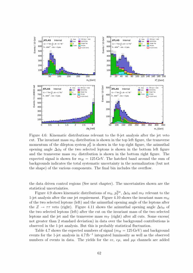
[GeV]llm
50 100 150 200 250
Eve
nts
/ 10
GeV
100
200
300
400
500
600
700 Data stat)⊕ SM (sys
WW γ WZ/ZZ/W
t t Single Top
Z+jets W+jets
H [125 GeV]
ATLAS Internal-1 L dt = 4.7 fb∫ = 7 TeV, s
+ 0 jetsνlνl→(*)WW→H
[GeV]llTP
0 20 40 60 80 100 120 140 160 180 200
Eve
nts
/ 10
GeV
100
200
300
400
500
600
700
800 Data stat)⊕ SM (sys
WW γ WZ/ZZ/W
t t Single Top
Z+jets W+jets
H [125 GeV]
ATLAS Internal-1 L dt = 4.7 fb∫ = 7 TeV, s
+ 0 jetsνlνl→(*)WW→H
[rad]ll
φ∆0 0.5 1 1.5 2 2.5 3
Eve
nts
/ 0.1
3083
3 ra
d
100
200
300
400
500
600
700
800
900 Data stat)⊕ SM (sys
WW γ WZ/ZZ/W
t t Single Top
Z+jets W+jets
H [125 GeV]
ATLAS Internal-1 L dt = 4.7 fb∫ = 7 TeV, s
+ 0 jetsνlνl→(*)WW→H
[GeV]Tm
50 100 150 200 250 300 350 400 450
Eve
nts
/ 10
GeV
100
200
300
400
500 Data stat)⊕ SM (sys
WW γ WZ/ZZ/W
t t Single Top
Z+jets W+jets
H [125 GeV]
ATLAS Internal-1 L dt = 4.7 fb∫ = 7 TeV, s
+ 0 jetsνlνl→(*)WW→H
Figure 4.6: Kinematic distributions relevant to the 0-jet analysis after the jet vetocut. The invariant mass mll distribution is shown in the top left figure, the transversemomentum of the dilepton system pll
T is shown in the top right figure, the azimuthalopening angle ∆φll of the two selected leptons is shown in the bottom left figureand the transverse mass mT distribution is shown in the bottom right figure. Theexpected signal is shown for mH = 125 GeV. The hatched band around the sum ofbackgrounds indicates the total systematic uncertainty in the normalization (but notthe shape) of the various components. The final bin includes the overflow.
the data driven control regions (See next chapter). The uncertainties shown are thestatistical uncertainties.
Figure 4.9 shows kinematic distributions of mll, pTotT , ∆φll and mT relevant to the
1-jet analysis after the one jet requirement. Figure 4.10 shows the invariant mass mℓℓ
of the two selected leptons (left) and the azimuthal opening angle of the leptons afterthe Z → ττ veto (right). Figure 4.11 shows the azimuthal opening angle ∆φℓℓ ofthe two selected leptons (left) after the cut on the invariant mass of the two selectedleptons and the jet and the transverse mass mT (right) after all cuts. Some excess(not greater than 2 standard deviation) in data over the background contributions isobserved in the 1-jet analysis. But this is probably statistical fluctuation.
Table 4.7 shows the expected numbers of signal (mH = 125 GeV) and backgroundevents for the 1-jet analysis in 4.7 fb−1 integrated luminosity as well as the observednumbers of events in data. The yields for the ee, eµ, and µµ channels are added
62
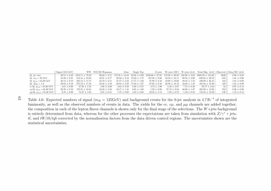
Signal [125 GeV] WW WZ/ZZ/Wgamma ttbar Single Top Z+jets W+jets (MC) W+jets (d-d) Total Bkg. (d-d) Observed Data/MC (d-d)
0j: jet veto 56.74 ± 0.23 1272.71 ± 79.34 96.62 ± 3.71 173.70 ± 12.16 94.92 ± 6.99 1038.66 ± 27.91 173.93 ± 20.94 216.98 ± 3.63 2893.59 ± 114.88 2849 0.98 ± 0.040j: mℓℓ < 50 GeV 45.22 ± 0.21 312.41 ± 19.64 40.81 ± 2.77 28.92 ± 2.34 19.23 ± 1.78 167.92 ± 9.60 56.42 ± 12.11 69.52 ± 2.00 638.83 ± 28.35 645 1.01 ± 0.060j: pT,ℓℓ >45,30 GeV 40.14 ± 0.19 282.12 ± 17.75 34.79 ± 2.51 27.27 ± 2.23 17.77 ± 1.68 27.98 ± 6.43 43.68 ± 10.60 49.16 ± 1.52 439.09 ± 26.44 443 1.01 ± 0.080j: ∆φℓℓ < 1.8 39.02 ± 0.19 275.54 ± 17.34 33.32 ± 2.43 26.83 ± 2.20 17.63 ± 1.67 27.65 ± 6.43 38.94 ± 10.12 44.08 ± 1.42 425.04 ± 25.99 429 1.01 ± 0.08ee:0j: pT,ℓℓ >45,30 GeV 4.01 ± 0.06 37.30 ± 2.52 4.08 ± 0.80 3.63 ± 0.56 3.29 ± 0.55 3.73 ± 1.90 5.46 ± 3.87 7.75 ± 0.38 59.77 ± 4.64 52 0.87 ± 0.14eµ:0j: pT,ℓℓ >45,30 GeV 26.76 ± 0.16 170.55 ± 10.81 24.50 ± 2.34 16.17 ± 1.45 9.65 ± 1.08 1.93 ± 0.80 37.19 ± 9.84 40.08 ± 1.37 262.89 ± 12.92 253 0.96 ± 0.08µµ:0j: pT,ℓℓ >45,30 GeV 9.37 ± 0.09 74.27 ± 4.82 6.21 ± 0.41 7.47 ± 0.80 4.83 ± 0.68 22.32 ± 5.13 1.03 ± 0.73 1.33 ± 0.54 116.43 ± 10.02 138 1.19 ± 0.14
Table 4.6: Expected numbers of signal (mH = 125GeV) and background events for the 0-jet analysis in 4.7 fb−1 of integratedluminosity, as well as the observed numbers of events in data. The yields for the ee, eµ, and µµ channels are added together,the composition in each of the lepton flavor channels is shown only for the final stage of the selections. The W+jets backgroundis entirely determined from data, whereas for the other processes the expectations are taken from simulation with Z/γ∗ + jets,tt, and tW/tb/tqb corrected by the normalisation factors from the data driven control regions. The uncertainties shown are thestatistical uncertainties.
63
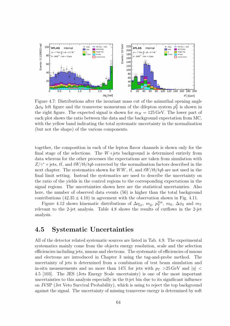
[rad]ll
φ∆0 0.5 1 1.5 2 2.5 3
Eve
nts
/ 0.1
3083
3 ra
d
20
40
60
80
100 Data stat)⊕ SM (sys
WW γ WZ/ZZ/W
t t Single Top
Z+jets W+jets
H [125 GeV]
ATLAS Internal-1 L dt = 4.7 fb∫ = 7 TeV, s
+ 0 jetsνlνl→(*)WW→H
[GeV]llTP
0 20 40 60 80 100 120 140 160 180 200
Eve
nts
/ 10
GeV
20406080
100120140160180200220 Data stat)⊕ SM (sys
WW γ WZ/ZZ/W
t t Single Top
Z+jets W+jets
H [125 GeV]
ATLAS Internal-1 L dt = 4.7 fb∫ = 7 TeV, s
+ 0 jetsνlνl→(*)WW→H
Figure 4.7: Distributions after the invariant mass cut of the azimuthal opening angle∆φll left figure and the transverse momentum of the dilepton system pll
T is shown inthe right figure. The expected signal is shown for mH = 125GeV. The lower part ofeach plot shows the ratio between the data and the background expectation from MC,with the yellow band indicating the total systematic uncertainty in the normalization(but not the shape) of the various components.
together, the composition in each of the lepton flavor channels is shown only for thefinal stage of the selections. The W+jets background is determined entirely fromdata whereas for the other processes the expectations are taken from simulation withZ/γ∗ +jets, tt, and tW/tb/tqb corrected by the normalisation factors described in thenext chapter. The systematics shown for WW , tt, and tW/tb/tqb are not used in thefinal limit setting. Instead the systematics are used to describe the uncertainty onthe ratio of the yields in the control regions to the corresponding expectations in thesignal regions. The uncertainties shown here are the statistical uncertainties. Alsohere, the number of observed data events (56) is higher than the total backgroundcontributions (42.35 ± 4.10) in agreement with the observation shown in Fig. 4.11.
Figure 4.12 shows kinematic distributions of ∆ηjj, mjj, pTotT , mll, ∆φll and mT
relevant to the 2-jet analysis. Table 4.8 shows the results of cutflows in the 2-jetanalysis.
4.5 Systematic Uncertainties
All of the detector related systematic sources are listed in Tab. 4.9. The experimentalsystematics mainly come from the objects energy resolution, scale and the selectionefficiencies including jets, muons and electrons. The systematic of efficiencies of muonsand electrons are introduced in Chapter 3 using the tag-and-probe method. Theuncertainty of jets is determined from a combination of test beam simulation andin-situ measurements and no more than 14% for jets with pT >25GeV and |η| <4.5 [103]. The JES (Jets Energy Scale uncertainty) is one of the most importantuncertainties to this analysis especially in the 0-jet bin due to its significant influenceon JVSP (Jet Veto Survival Probability), which is using to reject the top backgroundagainst the signal. The uncertainty of missing transverse energy is determined by soft
64
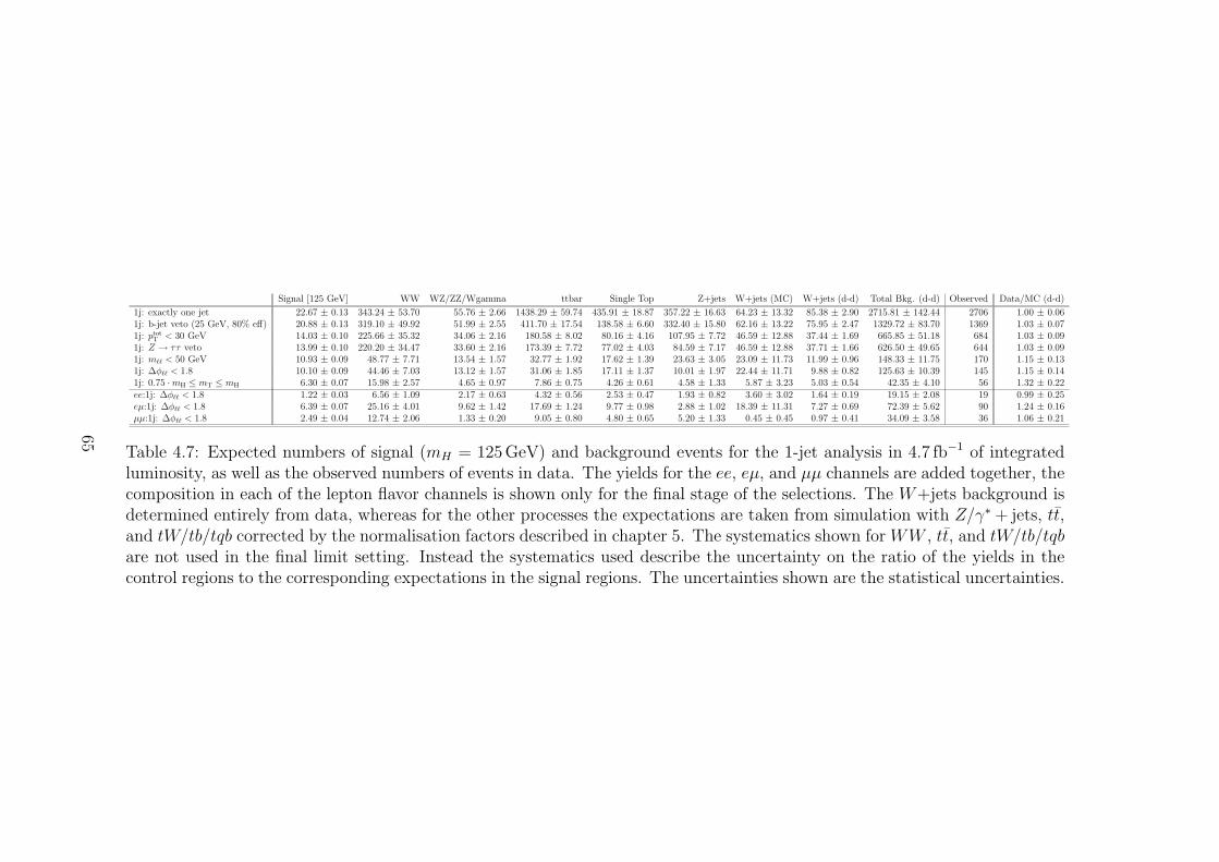
Signal [125 GeV] WW WZ/ZZ/Wgamma ttbar Single Top Z+jets W+jets (MC) W+jets (d-d) Total Bkg. (d-d) Observed Data/MC (d-d)
1j: exactly one jet 22.67 ± 0.13 343.24 ± 53.70 55.76 ± 2.66 1438.29 ± 59.74 435.91 ± 18.87 357.22 ± 16.63 64.23 ± 13.32 85.38 ± 2.90 2715.81 ± 142.44 2706 1.00 ± 0.061j: b-jet veto (25 GeV, 80% eff) 20.88 ± 0.13 319.10 ± 49.92 51.99 ± 2.55 411.70 ± 17.54 138.58 ± 6.60 332.40 ± 15.80 62.16 ± 13.22 75.95 ± 2.47 1329.72 ± 83.70 1369 1.03 ± 0.071j: ptot
T < 30 GeV 14.03 ± 0.10 225.66 ± 35.32 34.06 ± 2.16 180.58 ± 8.02 80.16 ± 4.16 107.95 ± 7.72 46.59 ± 12.88 37.44 ± 1.69 665.85 ± 51.18 684 1.03 ± 0.091j: Z → ττ veto 13.99 ± 0.10 220.20 ± 34.47 33.60 ± 2.16 173.39 ± 7.72 77.02 ± 4.03 84.59 ± 7.17 46.59 ± 12.88 37.71 ± 1.66 626.50 ± 49.65 644 1.03 ± 0.091j: mℓℓ < 50 GeV 10.93 ± 0.09 48.77 ± 7.71 13.54 ± 1.57 32.77 ± 1.92 17.62 ± 1.39 23.63 ± 3.05 23.09 ± 11.73 11.99 ± 0.96 148.33 ± 11.75 170 1.15 ± 0.131j: ∆φℓℓ < 1.8 10.10 ± 0.09 44.46 ± 7.03 13.12 ± 1.57 31.06 ± 1.85 17.11 ± 1.37 10.01 ± 1.97 22.44 ± 11.71 9.88 ± 0.82 125.63 ± 10.39 145 1.15 ± 0.141j: 0.75 ·mH ≤ mT ≤ mH 6.30 ± 0.07 15.98 ± 2.57 4.65 ± 0.97 7.86 ± 0.75 4.26 ± 0.61 4.58 ± 1.33 5.87 ± 3.23 5.03 ± 0.54 42.35 ± 4.10 56 1.32 ± 0.22ee:1j: ∆φℓℓ < 1.8 1.22 ± 0.03 6.56 ± 1.09 2.17 ± 0.63 4.32 ± 0.56 2.53 ± 0.47 1.93 ± 0.82 3.60 ± 3.02 1.64 ± 0.19 19.15 ± 2.08 19 0.99 ± 0.25eµ:1j: ∆φℓℓ < 1.8 6.39 ± 0.07 25.16 ± 4.01 9.62 ± 1.42 17.69 ± 1.24 9.77 ± 0.98 2.88 ± 1.02 18.39 ± 11.31 7.27 ± 0.69 72.39 ± 5.62 90 1.24 ± 0.16µµ:1j: ∆φℓℓ < 1.8 2.49 ± 0.04 12.74 ± 2.06 1.33 ± 0.20 9.05 ± 0.80 4.80 ± 0.65 5.20 ± 1.33 0.45 ± 0.45 0.97 ± 0.41 34.09 ± 3.58 36 1.06 ± 0.21
Table 4.7: Expected numbers of signal (mH = 125 GeV) and background events for the 1-jet analysis in 4.7 fb−1 of integratedluminosity, as well as the observed numbers of events in data. The yields for the ee, eµ, and µµ channels are added together, thecomposition in each of the lepton flavor channels is shown only for the final stage of the selections. The W+jets background isdetermined entirely from data, whereas for the other processes the expectations are taken from simulation with Z/γ∗ + jets, tt,and tW/tb/tqb corrected by the normalisation factors described in chapter 5. The systematics shown for WW , tt, and tW/tb/tqbare not used in the final limit setting. Instead the systematics used describe the uncertainty on the ratio of the yields in thecontrol regions to the corresponding expectations in the signal regions. The uncertainties shown are the statistical uncertainties.
65
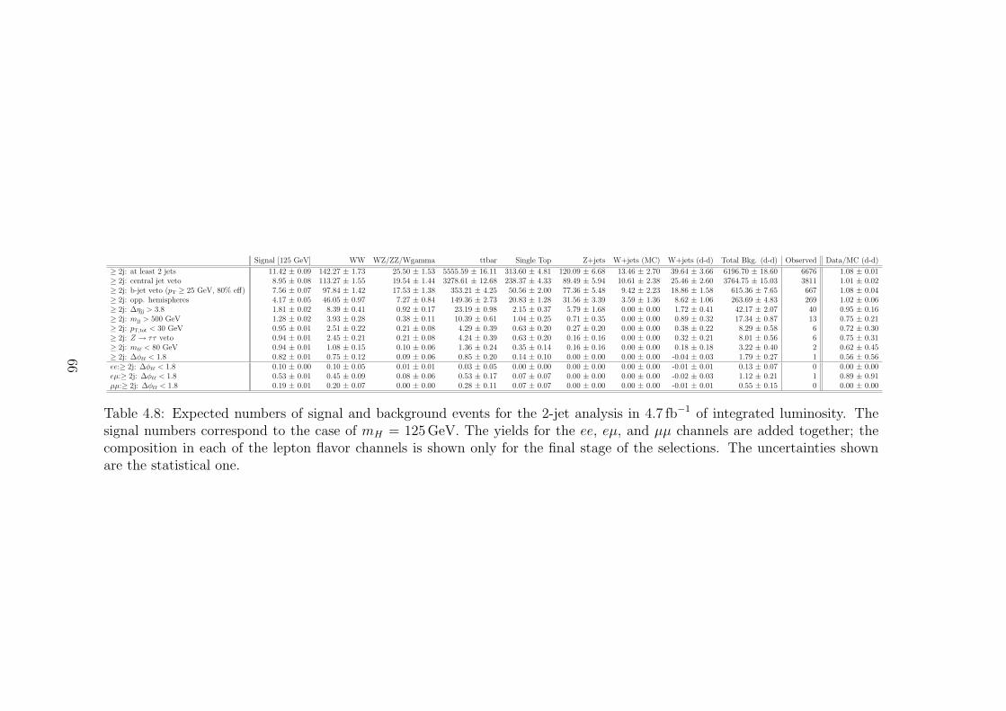
Signal [125 GeV] WW WZ/ZZ/Wgamma ttbar Single Top Z+jets W+jets (MC) W+jets (d-d) Total Bkg. (d-d) Observed Data/MC (d-d)
≥ 2j: at least 2 jets 11.42 ± 0.09 142.27 ± 1.73 25.50 ± 1.53 5555.59 ± 16.11 313.60 ± 4.81 120.09 ± 6.68 13.46 ± 2.70 39.64 ± 3.66 6196.70 ± 18.60 6676 1.08 ± 0.01≥ 2j: central jet veto 8.95 ± 0.08 113.27 ± 1.55 19.54 ± 1.44 3278.61 ± 12.68 238.37 ± 4.33 89.49 ± 5.94 10.61 ± 2.38 25.46 ± 2.60 3764.75 ± 15.03 3811 1.01 ± 0.02≥ 2j: b-jet veto (pT ≥ 25 GeV, 80% eff) 7.56 ± 0.07 97.84 ± 1.42 17.53 ± 1.38 353.21 ± 4.25 50.56 ± 2.00 77.36 ± 5.48 9.42 ± 2.23 18.86 ± 1.58 615.36 ± 7.65 667 1.08 ± 0.04≥ 2j: opp. hemispheres 4.17 ± 0.05 46.05 ± 0.97 7.27 ± 0.84 149.36 ± 2.73 20.83 ± 1.28 31.56 ± 3.39 3.59 ± 1.36 8.62 ± 1.06 263.69 ± 4.83 269 1.02 ± 0.06≥ 2j: ∆ηjj > 3.8 1.81 ± 0.02 8.39 ± 0.41 0.92 ± 0.17 23.19 ± 0.98 2.15 ± 0.37 5.79 ± 1.68 0.00 ± 0.00 1.72 ± 0.41 42.17 ± 2.07 40 0.95 ± 0.16≥ 2j: mjj > 500 GeV 1.28 ± 0.02 3.93 ± 0.28 0.38 ± 0.11 10.39 ± 0.61 1.04 ± 0.25 0.71 ± 0.35 0.00 ± 0.00 0.89 ± 0.32 17.34 ± 0.87 13 0.75 ± 0.21≥ 2j: pT,tot < 30 GeV 0.95 ± 0.01 2.51 ± 0.22 0.21 ± 0.08 4.29 ± 0.39 0.63 ± 0.20 0.27 ± 0.20 0.00 ± 0.00 0.38 ± 0.22 8.29 ± 0.58 6 0.72 ± 0.30≥ 2j: Z → ττ veto 0.94 ± 0.01 2.45 ± 0.21 0.21 ± 0.08 4.24 ± 0.39 0.63 ± 0.20 0.16 ± 0.16 0.00 ± 0.00 0.32 ± 0.21 8.01 ± 0.56 6 0.75 ± 0.31≥ 2j: mℓℓ < 80 GeV 0.94 ± 0.01 1.08 ± 0.15 0.10 ± 0.06 1.36 ± 0.24 0.35 ± 0.14 0.16 ± 0.16 0.00 ± 0.00 0.18 ± 0.18 3.22 ± 0.40 2 0.62 ± 0.45≥ 2j: ∆φℓℓ < 1.8 0.82 ± 0.01 0.75 ± 0.12 0.09 ± 0.06 0.85 ± 0.20 0.14 ± 0.10 0.00 ± 0.00 0.00 ± 0.00 -0.04 ± 0.03 1.79 ± 0.27 1 0.56 ± 0.56ee:≥ 2j: ∆φℓℓ < 1.8 0.10 ± 0.00 0.10 ± 0.05 0.01 ± 0.01 0.03 ± 0.05 0.00 ± 0.00 0.00 ± 0.00 0.00 ± 0.00 -0.01 ± 0.01 0.13 ± 0.07 0 0.00 ± 0.00eµ:≥ 2j: ∆φℓℓ < 1.8 0.53 ± 0.01 0.45 ± 0.09 0.08 ± 0.06 0.53 ± 0.17 0.07 ± 0.07 0.00 ± 0.00 0.00 ± 0.00 -0.02 ± 0.03 1.12 ± 0.21 1 0.89 ± 0.91µµ:≥ 2j: ∆φℓℓ < 1.8 0.19 ± 0.01 0.20 ± 0.07 0.00 ± 0.00 0.28 ± 0.11 0.07 ± 0.07 0.00 ± 0.00 0.00 ± 0.00 -0.01 ± 0.01 0.55 ± 0.15 0 0.00 ± 0.00
Table 4.8: Expected numbers of signal and background events for the 2-jet analysis in 4.7 fb−1 of integrated luminosity. Thesignal numbers correspond to the case of mH = 125 GeV. The yields for the ee, eµ, and µµ channels are added together; thecomposition in each of the lepton flavor channels is shown only for the final stage of the selections. The uncertainties shownare the statistical one.
66
[GeV]llTP
0 20 40 60 80 100 120 140 160 180 200
Eve
nts
/ 10
GeV
20
40
60
80
100
120
140
160
180
200 Data stat)⊕ SM (sys
WW γ WZ/ZZ/W
t t Single Top
Z+jets W+jets
H [125 GeV]
ATLAS Internal-1 L dt = 4.7 fb∫ = 7 TeV, s
+ 0 jetsνlνl→(*)
WW→H
[GeV]Tm
60 80 100 120 140 160 180 200 220 240
Eve
nts
/ 10
GeV
20
40
60
80
100
120 Data stat)⊕ SM (sys
WW γ WZ/ZZ/W
t t Single Top
Z+jets W+jets
H [125 GeV]
ATLAS Internal-1 L dt = 4.7 fb∫ = 7 TeV, s
+ 0 jetsνlνl→(*)WW→H
Figure 4.8: Transverse momentum pllT of the two selected leptons is shown in the left
figure after the cut on the azimuthal opening angle ∆φll and the transverse mass mT
distribution is shown in the right figure after all cuts. The expected signal is shownin both plots for mH = 125 GeV. The hatched band around the sum of backgroundsindicates the total systematic uncertainty in the normalization (but not the shape)of the various components. The final bin includes the overflow.
calorimeter energy deposits and all of the uncertainties which are propagated to theEmiss
T calculation. In addition, when a b-tagging is needed, the b-jet tagging efficiencyuncertainty is introduced by varying the efficiency between 5% and 14% as a functionof jet pT [81]. The uncertainty on the integrated luminosity in 2011 is 3.9% [104].
67
[GeV]llm
50 100 150 200 250
Eve
nts
/ 10
GeV
50
100
150
200
250
300
350
400
450 Data stat)⊕ SM (sys
WW γ WZ/ZZ/W
t t Single Top
Z+jets W+jets
H [125 GeV]
ATLAS Internal-1 L dt = 4.7 fb∫ = 7 TeV, s
+ 1 jetνlνl→(*)WW→H
[GeV]TotTP
0 10 20 30 40 50 60 70 80
Eve
nts
/ 5 G
eV
100
200
300
400
500 Data stat)⊕ SM (sys
WW γ WZ/ZZ/W
t t Single Top
Z+jets W+jets
H [125 GeV]
ATLAS Internal-1 L dt = 4.7 fb∫ = 7 TeV, s
+ 1 jetνlνl→(*)WW→H
[rad]ll
φ∆0 0.5 1 1.5 2 2.5 3
Eve
nts
/ 0.1
3083
3 ra
d
50
100
150
200
250
300 Data stat)⊕ SM (sys
WW γ WZ/ZZ/W
t t Single Top
Z+jets W+jets
H [125 GeV]
ATLAS Internal-1 L dt = 4.7 fb∫ = 7 TeV, s
+ 1 jetνlνl→(*)WW→H
[GeV]Tm
50 100 150 200 250 300 350 400 450
Eve
nts
/ 10
GeV
50
100
150
200
250
300 Data stat)⊕ SM (sys
WW γ WZ/ZZ/W
t t Single Top
Z+jets W+jets
H [125 GeV]
ATLAS Internal-1 L dt = 4.7 fb∫ = 7 TeV, s
+ 1 jetνlνl→(*)WW→H
Figure 4.9: Kinematic distributions relevant to the 1-jet analysis after the one jetrequirement has been applied: dilepton invariant mass (top left), total transversemomentum (top right), and azimuthal opening angle (bottom left) transverse mass(bottom left). The expected signal is shown for mH = 125 GeV. The hatched bandaround the sum of backgrounds indicates the total systematic uncertainty in thenormalization (but not the shape) of the various components. The final bin includesthe overflow.
68
[GeV]llm
50 100 150 200 250
Eve
nts
/ 10
GeV
20
40
60
80
100
120 Data stat)⊕ SM (sys
WW γ WZ/ZZ/W
t t Single Top
Z+jets W+jets
H [125 GeV]
ATLAS Internal-1 L dt = 4.7 fb∫ = 7 TeV, s
+ 1 jetνlνl→(*)WW→H
[rad]ll
φ∆0 0.5 1 1.5 2 2.5 3
Eve
nts
/ 0.1
3083
3 ra
d
10
20
30
40
50
60
70 Data stat)⊕ SM (sys
WW γ WZ/ZZ/W
t t Single Top
Z+jets W+jets
H [125 GeV]
ATLAS Internal-1 L dt = 4.7 fb∫ = 7 TeV, s
+ 1 jetνlνl→(*)WW→H
Figure 4.10: The invariant mass mℓℓ of the two selected leptons (left) and the az-imuthal opening angle of the leptons after the Z → ττ veto (right). The expectedsignal is shown in both plots for mH = 125 GeV. The hatched band around the sumof backgrounds indicates the total systematic uncertainty in the normalization (butnot the shape) of the various components. The final bin includes the overflow.
[rad]ll
φ∆0 0.5 1 1.5 2 2.5 3
Eve
nts
/ 0.1
3083
3 ra
d
5
10
15
20
25
30 Data stat)⊕ SM (sys
WW γ WZ/ZZ/W
t t Single Top
Z+jets W+jets
H [125 GeV]
ATLAS Internal-1 L dt = 4.7 fb∫ = 7 TeV, s
+ 1 jetνlνl→(*)WW→H
[GeV]Tm
60 80 100 120 140 160 180 200 220 240
Eve
nts
/ 10
GeV
5
10
15
20
25
30
35 Data stat)⊕ SM (sys
WW γ WZ/ZZ/W
t t Single Top
Z+jets W+jets
H [125 GeV]
ATLAS Internal-1 L dt = 4.7 fb∫ = 7 TeV, s
+ 1 jetνlνl→(*)WW→H
Figure 4.11: Azimuthal opening angle ∆φℓℓ of the two selected leptons (left) after thecut on the invariant mass of the two selected leptons and the jet and the transversemass (right) after all cuts. The expected signal is shown for mH = 125GeV. Thehatched band around the sum of backgrounds indicates the total systematic uncer-tainty in the normalization (but not the shape) of the various components. The finalbin includes the overflow.
69
jjη∆
0 0.5 1 1.5 2 2.5 3 3.5 4 4.5 5
Eve
nts
/ 0.1
6666
7
100
200
300
400
500 Data stat)⊕ SM (sys
WW γ WZ/ZZ/W
t t Single Top
Z+jets W+jets
H [125 GeV]
ATLAS Internal-1 L dt = 4.7 fb∫ = 7 TeV, s
2 jets≥ + νlνl→(*)WW→H
[GeV]jjm
0 100 200 300 400 500 600
Eve
nts
/ 20
GeV
20
40
60
80
100
120 Data stat)⊕ SM (sys
WW γ WZ/ZZ/W
t t Single Top
Z+jets W+jets
H [125 GeV]
ATLAS Internal-1 L dt = 4.7 fb∫ = 7 TeV, s
2 jets≥ + νlνl→(*)WW→H
[GeV]TotTP
0 10 20 30 40 50 60 70 80
Eve
nts
/ 5 G
eV
2
4
6
8
10
12
14 Data stat)⊕ SM (sys
WW γ WZ/ZZ/W
t t Single Top
Z+jets W+jets
H [125 GeV]
ATLAS Internal-1 L dt = 4.7 fb∫ = 7 TeV, s
2 jets≥ + νlνl→(*)WW→H
[GeV]llm
50 100 150 200 250
Eve
nts
/ 10
GeV
2
4
6
8
10
12
14
16 Data stat)⊕ SM (sys
WW γ WZ/ZZ/W
t t Single Top
Z+jets W+jets
H [125 GeV]
ATLAS Internal-1 L dt = 4.7 fb∫ = 7 TeV, s
2 jets≥ + νlνl→(*)WW→H
[rad]ll
φ∆0 0.5 1 1.5 2 2.5 3
Eve
nts
/ 0.1
3083
3 ra
d
2
4
6
8
10
12 Data stat)⊕ SM (sys
WW γ WZ/ZZ/W
t t Single Top
Z+jets W+jets
H [125 GeV]
ATLAS Internal-1 L dt = 4.7 fb∫ = 7 TeV, s
2 jets≥ + νlνl→(*)WW→H
[GeV]Tm
50 100 150 200 250 300 350 400 450
Eve
nts
/ 10
GeV
2
4
6
8
10
12 Data stat)⊕ SM (sys
WW γ WZ/ZZ/W
t t Single Top
Z+jets W+jets
H [125 GeV]
ATLAS Internal-1 L dt = 4.7 fb∫ = 7 TeV, s
2 jets≥ + νlνl→(*)WW→H
Figure 4.12: Kinematic distributions relevant to the 2-jet analysis. Top: ∆ηjj afterrequiring that the two leading jets are in opposite hemispheres. Upper right: mjj
after the cut on ∆ηjj. The remaining plots are shown after the Central Jet Veto cut.Middle left: the distribution of pTot
T . Middle right: the distribution of ∆φll. Lowerleft: the distribution of the dilepton invariant mass. Lower right: the distribution ofmT. The expected signal is shown for mH = 125 GeV. The hatched band around thesum of backgrounds indicates the total systematic uncertainty in the normalization(but not the shape) of the various components. The final bin includes the overflow.
70
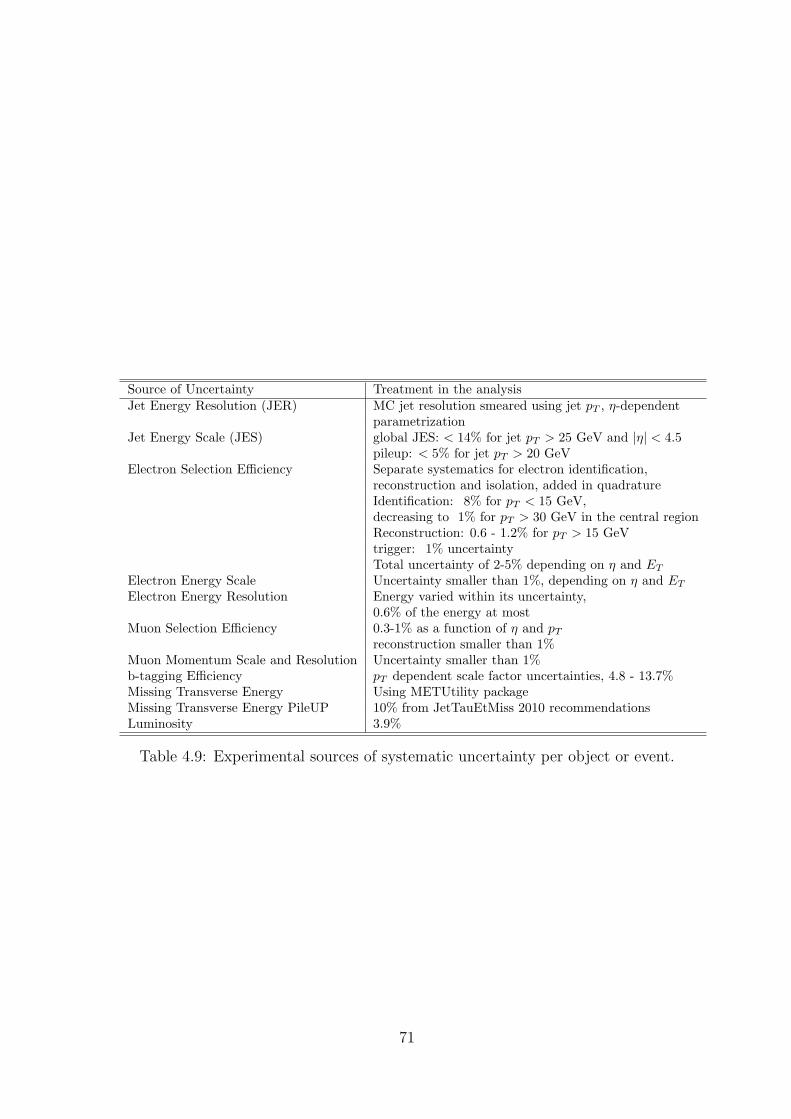
Source of Uncertainty Treatment in the analysisJet Energy Resolution (JER) MC jet resolution smeared using jet pT , η-dependent
parametrizationJet Energy Scale (JES) global JES: < 14% for jet pT > 25 GeV and |η| < 4.5
pileup: < 5% for jet pT > 20 GeVElectron Selection Efficiency Separate systematics for electron identification,
reconstruction and isolation, added in quadratureIdentification: 8% for pT < 15 GeV,decreasing to 1% for pT > 30 GeV in the central regionReconstruction: 0.6 - 1.2% for pT > 15 GeVtrigger: 1% uncertaintyTotal uncertainty of 2-5% depending on η and ET
Electron Energy Scale Uncertainty smaller than 1%, depending on η and ET
Electron Energy Resolution Energy varied within its uncertainty,0.6% of the energy at most
Muon Selection Efficiency 0.3-1% as a function of η and pT
reconstruction smaller than 1%Muon Momentum Scale and Resolution Uncertainty smaller than 1%b-tagging Efficiency pT dependent scale factor uncertainties, 4.8 - 13.7%Missing Transverse Energy Using METUtility packageMissing Transverse Energy PileUP 10% from JetTauEtMiss 2010 recommendationsLuminosity 3.9%
Table 4.9: Experimental sources of systematic uncertainty per object or event.
71

72
Chapter 5
Background Estimation
5.1 Introduction
In the H → WW (∗) → lνlν analysis as in other Higgs search analyses, it is extremelyimportant to estimate reliably the background contributions. Therefore, whenever itis possible, data-driven methods are designed and used either to replace the corre-sponding MC prediction or to check the MC prediction both on the normalisationand on the shape of the relevant kinematic distributions.
In the Higgs to WW (∗) analysis, the main backgrounds are QCD(multijet or di-jet), W+jets, Z+jets, top, and the Standard Model diboson processes: WW , WZ,ZZ and Wγ. QCD is strongly suppressed to a negligible level by the requirementof two very tight isolated leptons, the 0-jet veto selection and the Emiss
T cut [107].The W+jet events have a huge initial rate and can not be reliably simulated withsufficiently large MC sample. It is thus derived fully from data. The Z+jets can besuppressed by the Z mass peak veto and the Emiss
T and pllT cuts. However, the shape
of the EmissT distribution is very sensitive to the pile up effects in 2011 and especially
in 2012 high luminosity data taking periods. Any mismodelling of the EmissT affects
the final estimate of the Z+jets contribution. A data-driven method is needed tocorrect such mismodelling of the Emiss
T . The top events have two isolated leptons andlarge Emiss
T associated with two additional b jets. It can be suppressed by jet vetocut in the 0-jet analysis or b-jet veto in 1- and 2-jet bins. However, the jet energyscale uncertainty is the most significant experimental systematic uncertainty, whichcan vary up to 20% in rejecting the top background. So a data-driven method withreduced sensitivity to the JES variation is essential. The Standard Model WW is anirreducible background which has the same topology as the signal. The correspondingMC prediction, though fairly reliable, is verified using a dedicated control regionselected from the dilepton invariant mass spectrum far away from the Higgs signalregion. For the other backgrounds, either they are negligible or the MC predictionsare checked to be reliable.
In this chapter, the data driven methods to estimate W+jets, top, Z+jets aredescribed and discussed in detail in some cases to which we have directly contributed.
73
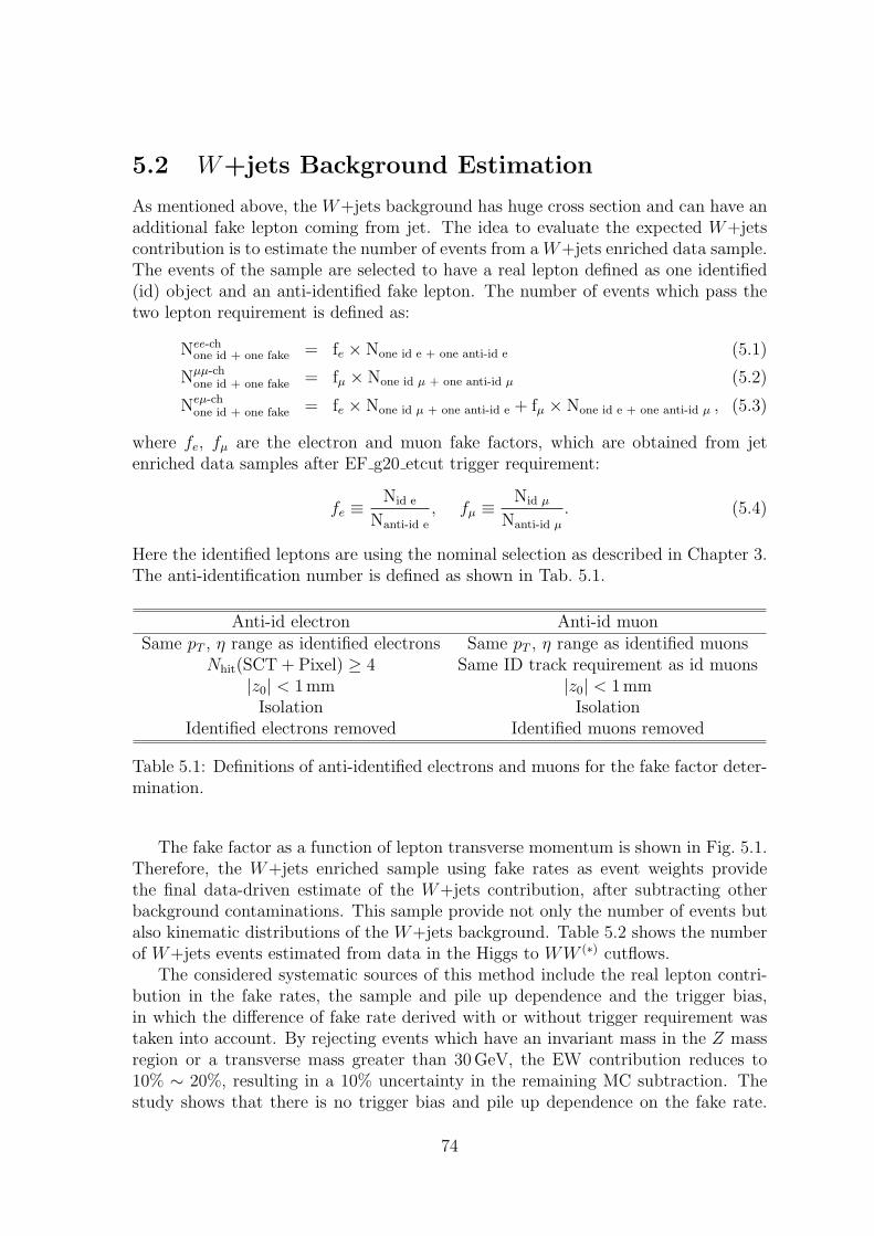
5.2 W+jets Background Estimation
As mentioned above, the W+jets background has huge cross section and can have anadditional fake lepton coming from jet. The idea to evaluate the expected W+jetscontribution is to estimate the number of events from a W+jets enriched data sample.The events of the sample are selected to have a real lepton defined as one identified(id) object and an anti-identified fake lepton. The number of events which pass thetwo lepton requirement is defined as:
Nee-chone id + one fake = fe × None id e + one anti-id e (5.1)
Nµµ-chone id + one fake = fµ × None id µ + one anti-id µ (5.2)
Neµ-chone id + one fake = fe × None id µ + one anti-id e + fµ × None id e + one anti-id µ , (5.3)
where fe, fµ are the electron and muon fake factors, which are obtained from jetenriched data samples after EF g20 etcut trigger requirement:
fe ≡Nid e
Nanti-id e
, fµ ≡ Nid µ
Nanti-id µ
. (5.4)
Here the identified leptons are using the nominal selection as described in Chapter 3.The anti-identification number is defined as shown in Tab. 5.1.
Anti-id electron Anti-id muonSame pT , η range as identified electrons Same pT , η range as identified muons
Nhit(SCT + Pixel) ≥ 4 Same ID track requirement as id muons|z0| < 1 mm |z0| < 1 mm
Isolation IsolationIdentified electrons removed Identified muons removed
Table 5.1: Definitions of anti-identified electrons and muons for the fake factor deter-mination.
The fake factor as a function of lepton transverse momentum is shown in Fig. 5.1.Therefore, the W+jets enriched sample using fake rates as event weights providethe final data-driven estimate of the W+jets contribution, after subtracting otherbackground contaminations. This sample provide not only the number of events butalso kinematic distributions of the W+jets background. Table 5.2 shows the numberof W+jets events estimated from data in the Higgs to WW (∗) cutflows.
The considered systematic sources of this method include the real lepton contri-bution in the fake rates, the sample and pile up dependence and the trigger bias,in which the difference of fake rate derived with or without trigger requirement wastaken into account. By rejecting events which have an invariant mass in the Z massregion or a transverse mass greater than 30 GeV, the EW contribution reduces to10% ∼ 20%, resulting in a 10% uncertainty in the remaining MC subtraction. Thestudy shows that there is no trigger bias and pile up dependence on the fake rate.
74
[GeV]T
p
0 20 40 60 80 100120140160180200
Ele
ctro
n F
ake
Fac
tor
0
0.01
0.02
0.03
0.04
0.05
0.06
0.07
0.08
0.09
0.1
electron fakeStat Only+Real Lepton Contamination+Run Dependence+Sample Dependence+Trigger Bias (total)
-1 Ldt = 1.46pb∫
[GeV]T
p
0 20 40 60 80 100120140160180200
Muo
n F
ake
Fac
tor
0
0.1
0.2
0.3
0.4
0.5
0.6
0.7
0.8
0.9
1
muon fakeStat Only+Real Lepton Contamination+Run Dependence+Sample Dependence+Trigger Bias (total)
-1 Ldt = 1.46pb∫
Figure 5.1: Fake factor as a function of pT including all systematic uncertainties forelectrons (left) and muons (right). This trigger is highly prescaled and the equivalentluminosity is 1.46 pb−1 using the full 2011 data set.
The difference of fake rate derived from different MC samples, dijet or W+jets, gives20% ∼ 50% variation depending on pT .
The result can be validated with the same sign event sample. In this same signsample, the contamination from other non W+jets backgrounds is small so thatW+jets have a high puirty. Good agreement is observed between data and MC inthe shapes of kinematic distributions, as shown in Fig. 5.2. Using this method, theW+jet background estimate is not statistically limited contrary to the correspondingMC prediction.
5.3 Top Background Estimation
After the common event selection (Section 4.4.1), the top background is the dominantcontribution in the inclusive event sample having two isolated leptons and large Emiss
T .It accounts for a small contribution in the total backgrounds in the 0-jet bin butdominates in the 1- and 2-jet bins. The number of top events in the 0-jet analysis,however, is directly proportional to the full Jet Veto Survival Probability (jet vetoefficiency, JVSP). Studies based on top MC simulations show that JVSP is subject tovarious systematic variation such as JES, JER and pile up. Therefore, it is necessaryto design a method to estimate reliably the top contribution in 0-jet channel withreduced sensitivities to different systematic variations [111].
5.3.1 Description of the Top Process
The inclusive process pp → W+W−bb with subsequent W decays gives rise to thesame leptonic final state with Emiss
T as the Higgs signal events. The phase space of theinclusive process may be divided into three parts corresponding to double resonance
75
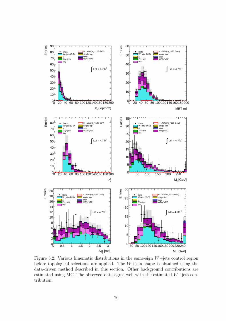
(lepton2)TP
0 20 40 60 80 100120140160180200
Ent
ries
0
10
20
30
40
50
60
70
80
90
-1 Ldt = 4.7fb∫
Data =125 GeV)H
WW(m→HW+jets (D-D) single toptt WW
+jetsγZ/ *)/ZZγWZ(γW
MET rel
0 20 40 60 80 100120140160180200
Ent
ries
0
10
20
30
40
50
60
-1 Ldt = 4.7fb∫
Data =125 GeV)H
WW(m→HW+jets (D-D) single toptt WW
+jetsγZ/ *)/ZZγWZ(γW
llTP
0 20 40 60 80 100120140160180200
Ent
ries
0
10
20
30
40
50
60
70
80
-1 Ldt = 4.7fb∫
Data =125 GeV)H
WW(m→HW+jets (D-D) single toptt WW
+jetsγZ/ *)/ZZγWZ(γW
[GeV]llM
50 100 150 200 250
Ent
ries
0
5
10
15
20
25
30
35
-1 Ldt = 4.7fb∫
Data =125 GeV)H
WW(m→HW+jets (D-D) single toptt WW
+jetsγZ/ *)/ZZγWZ(γW
[rad]ll
φ∆0 0.5 1 1.5 2 2.5 3
Ent
ries
0
2
4
6
8
10
12
14
16
18
20
-1 Ldt = 4.7fb∫
Data =125 GeV)H
WW(m→HW+jets (D-D) single toptt WW
+jetsγZ/ *)/ZZγWZ(γW
[GeV]TM
60 80 100120140160180200220240
Ent
ries
0
5
10
15
20
25
30
-1 Ldt = 4.7fb∫
Data =125 GeV)H
WW(m→HW+jets (D-D) single toptt WW
+jetsγZ/ *)/ZZγWZ(γW
Figure 5.2: Various kinematic distributions in the same-sign W+jets control regionbefore topological selections are applied. The W+jets shape is obtained using thedata-driven method described in this section. Other background contributions areestimated using MC. The observed data agree well with the estimated W+jets con-tribution.
76
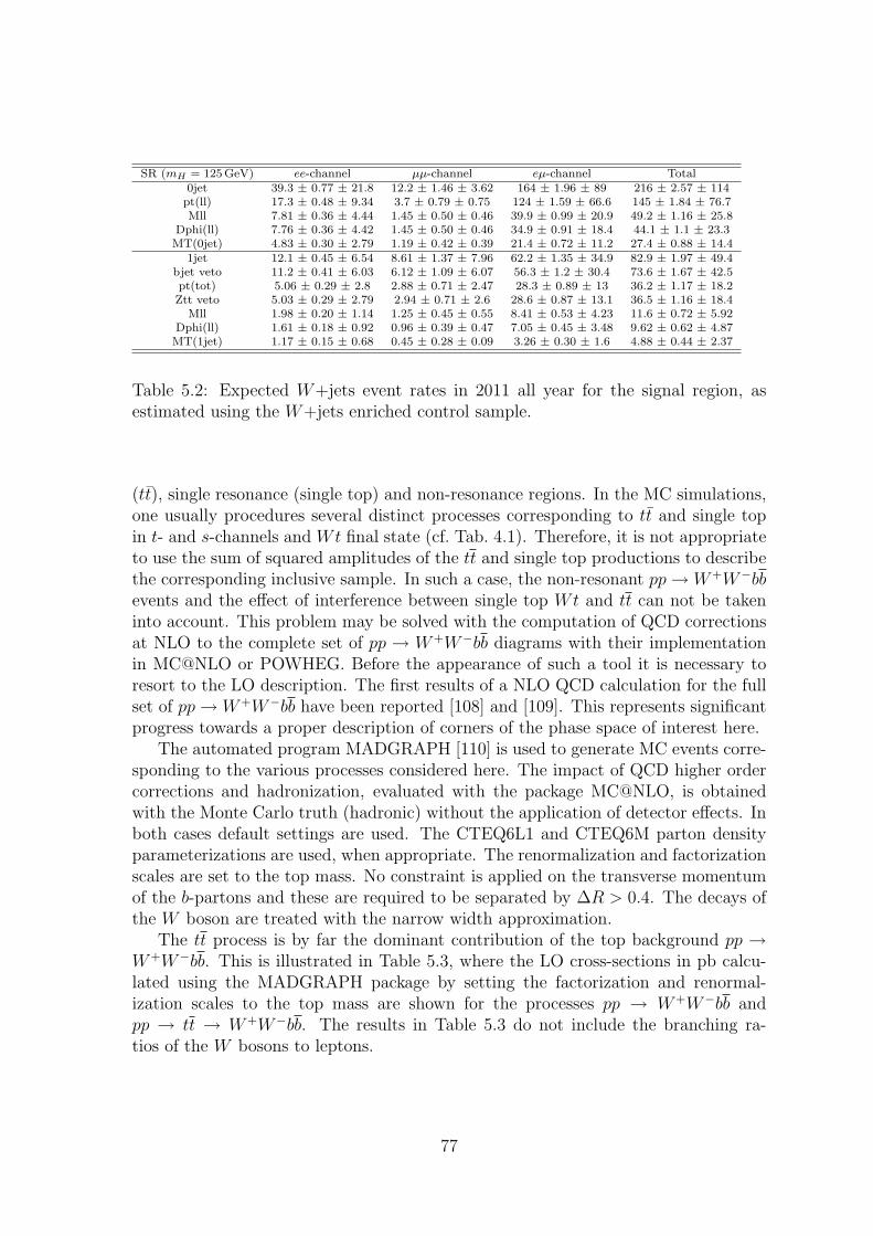
SR (mH = 125GeV) ee-channel µµ-channel eµ-channel Total0jet 39.3 ± 0.77 ± 21.8 12.2 ± 1.46 ± 3.62 164 ± 1.96 ± 89 216 ± 2.57 ± 114pt(ll) 17.3 ± 0.48 ± 9.34 3.7 ± 0.79 ± 0.75 124 ± 1.59 ± 66.6 145 ± 1.84 ± 76.7Mll 7.81 ± 0.36 ± 4.44 1.45 ± 0.50 ± 0.46 39.9 ± 0.99 ± 20.9 49.2 ± 1.16 ± 25.8
Dphi(ll) 7.76 ± 0.36 ± 4.42 1.45 ± 0.50 ± 0.46 34.9 ± 0.91 ± 18.4 44.1 ± 1.1 ± 23.3MT(0jet) 4.83 ± 0.30 ± 2.79 1.19 ± 0.42 ± 0.39 21.4 ± 0.72 ± 11.2 27.4 ± 0.88 ± 14.4
1jet 12.1 ± 0.45 ± 6.54 8.61 ± 1.37 ± 7.96 62.2 ± 1.35 ± 34.9 82.9 ± 1.97 ± 49.4bjet veto 11.2 ± 0.41 ± 6.03 6.12 ± 1.09 ± 6.07 56.3 ± 1.2 ± 30.4 73.6 ± 1.67 ± 42.5pt(tot) 5.06 ± 0.29 ± 2.8 2.88 ± 0.71 ± 2.47 28.3 ± 0.89 ± 13 36.2 ± 1.17 ± 18.2Ztt veto 5.03 ± 0.29 ± 2.79 2.94 ± 0.71 ± 2.6 28.6 ± 0.87 ± 13.1 36.5 ± 1.16 ± 18.4
Mll 1.98 ± 0.20 ± 1.14 1.25 ± 0.45 ± 0.55 8.41 ± 0.53 ± 4.23 11.6 ± 0.72 ± 5.92Dphi(ll) 1.61 ± 0.18 ± 0.92 0.96 ± 0.39 ± 0.47 7.05 ± 0.45 ± 3.48 9.62 ± 0.62 ± 4.87MT(1jet) 1.17 ± 0.15 ± 0.68 0.45 ± 0.28 ± 0.09 3.26 ± 0.30 ± 1.6 4.88 ± 0.44 ± 2.37
Table 5.2: Expected W+jets event rates in 2011 all year for the signal region, asestimated using the W+jets enriched control sample.
(tt), single resonance (single top) and non-resonance regions. In the MC simulations,one usually procedures several distinct processes corresponding to tt and single topin t- and s-channels and Wt final state (cf. Tab. 4.1). Therefore, it is not appropriateto use the sum of squared amplitudes of the tt and single top productions to describethe corresponding inclusive sample. In such a case, the non-resonant pp→ W+W−bbevents and the effect of interference between single top Wt and tt can not be takeninto account. This problem may be solved with the computation of QCD correctionsat NLO to the complete set of pp → W+W−bb diagrams with their implementationin MC@NLO or POWHEG. Before the appearance of such a tool it is necessary toresort to the LO description. The first results of a NLO QCD calculation for the fullset of pp→ W+W−bb have been reported [108] and [109]. This represents significantprogress towards a proper description of corners of the phase space of interest here.
The automated program MADGRAPH [110] is used to generate MC events corre-sponding to the various processes considered here. The impact of QCD higher ordercorrections and hadronization, evaluated with the package MC@NLO, is obtainedwith the Monte Carlo truth (hadronic) without the application of detector effects. Inboth cases default settings are used. The CTEQ6L1 and CTEQ6M parton densityparameterizations are used, when appropriate. The renormalization and factorizationscales are set to the top mass. No constraint is applied on the transverse momentumof the b-partons and these are required to be separated by ∆R > 0.4. The decays ofthe W boson are treated with the narrow width approximation.
The tt process is by far the dominant contribution of the top background pp →W+W−bb. This is illustrated in Table 5.3, where the LO cross-sections in pb calcu-lated using the MADGRAPH package by setting the factorization and renormal-ization scales to the top mass are shown for the processes pp → W+W−bb andpp → tt → W+W−bb. The results in Table 5.3 do not include the branching ra-tios of the W bosons to leptons.
77
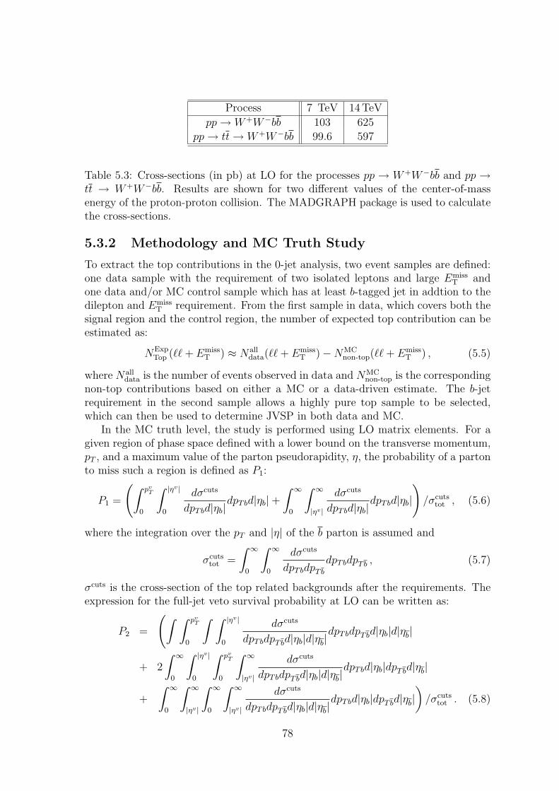
Process 7 TeV 14TeV
pp→ W+W−bb 103 625
pp→ tt→ W+W−bb 99.6 597
Table 5.3: Cross-sections (in pb) at LO for the processes pp → W+W−bb and pp →tt → W+W−bb. Results are shown for two different values of the center-of-massenergy of the proton-proton collision. The MADGRAPH package is used to calculatethe cross-sections.
5.3.2 Methodology and MC Truth Study
To extract the top contributions in the 0-jet analysis, two event samples are defined:one data sample with the requirement of two isolated leptons and large Emiss
T andone data and/or MC control sample which has at least b-tagged jet in addtion to thedilepton and Emiss
T requirement. From the first sample in data, which covers both thesignal region and the control region, the number of expected top contribution can beestimated as:
NExpTop (ℓℓ+ Emiss
T ) ≈ Nalldata(ℓℓ+ Emiss
T ) −NMCnon-top(ℓℓ+ Emiss
T ) , (5.5)
where Nalldata is the number of events observed in data and NMC
non-top is the correspondingnon-top contributions based on either a MC or a data-driven estimate. The b-jetrequirement in the second sample allows a highly pure top sample to be selected,which can then be used to determine JVSP in both data and MC.
In the MC truth level, the study is performed using LO matrix elements. For agiven region of phase space defined with a lower bound on the transverse momentum,pT , and a maximum value of the parton pseudorapidity, η, the probability of a partonto miss such a region is defined as P1:
P1 =
(
∫ pvT
0
∫ |ηv |
0
dσcuts
dpTbd|ηb|dpTbd|ηb| +
∫ ∞
0
∫ ∞
|ηv |
dσcuts
dpTbd|ηb|dpTbd|ηb|
)
/σcutstot , (5.6)
where the integration over the pT and |η| of the b parton is assumed and
σcutstot =
∫ ∞
0
∫ ∞
0
dσcuts
dpTbdpTb
dpTbdpTb , (5.7)
σcuts is the cross-section of the top related backgrounds after the requirements. Theexpression for the full-jet veto survival probability at LO can be written as:
P2 =
(
∫ ∫ pvT
0
∫ ∫ |ηv |
0
dσcuts
dpTbdpTbd|ηb|d|ηb|dpTbdpTbd|ηb|d|ηb|
+ 2
∫ ∞
0
∫ |ηv |
0
∫ pvT
0
∫ ∞
|ηv |
dσcuts
dpTbdpTbd|ηb|d|ηb|dpTbd|ηb|dpTbd|ηb|
+
∫ ∞
0
∫ ∞
|ηv |
∫ ∞
0
∫ ∞
|ηv |
dσcuts
dpTbdpTbd|ηb|d|ηb|dpTbd|ηb|dpTbd|ηb|
)
/σcutstot . (5.8)
78
It is important to note that the second term in Expression (5.6) and the last twoterms in Expression (5.8) become significantly smaller than the first terms for valuesof |ηv| > 3. These terms become negligible for |ηv| > 4.
The survival probability relevant to the second control sample is defined as:
PBtag1 =
(
∫ pvT
0
∫ |ηv |
0
dσBtag
dpTd|η|dpTd|η| +
∫ ∞
0
∫ ∞
|ηv |
dσBtag
dpTd|η|dpTd|η|
)
/σBtagtot , (5.9)
where dσBtag
dpT d|η|and σBtag
tot are the double differential and the total cross-section with therequirement that the event has at least one b-tagged parton. It is worth noting thatthe second term in Expression (5.9) is significantly smaller than the first.
The measured probability PBtag,Exp1 can be obtained from the reconstructed probe
jet multiplicity distribution in the b-tagged control sample by
PBtag,Exp1 =
NExpTop (ℓℓ+ Emiss
T + b-tagged, 0j)
NExpTop (ℓℓ+ Emiss
T + b-tagged)(5.10)
where the denominator is the total number of events of the b-tagged samples and thenumerator refers to the number of events having zero probe jet. The probe jet isdefined as follows:
• Consider all jets reconstructed with the nominal jet selection in each event withat least one tagged b-jet,
• For events with more than one tagged b-jets, select the b-jet which has thelargest b-tagged weight,
• Any remaining jet is counted as a probe jet if it has a ∆R with the b-tagged jetgreater than 1.
For the LO parton level study performed in [111], the b parton is tagged using arandom number as there are always two b parton in a top event.
The corresponding experimental full-jet veto survival probability PExp2 can be
derived using the jet multiplicity distribution:
PExp2 =
NExpTop (ℓℓ+ Emiss
T , 0j)
NExpTop (ℓℓ+ Emiss
T )(5.11)
where the numerator and the denominator are the number of top background eventsafter the application of a full-jet veto and the total number of top background eventswithout the application of any requirements on the jet multiplicity in the final state,respectively.
When these probabilities are much smaller than one for low pT thresholds, one canassume PExp
2 ≈ ǫ20P2 and PBtag,Exp1 ≈ ǫ0P
Btag1 where ǫ0 is an experimental efficiency of
observing a low pT jet in the region of interest. These relations may be rewritten as
PExp2
(
PBtag,Exp1
)2 ≈ P2(
PBtag1
)2 . (5.12)
79
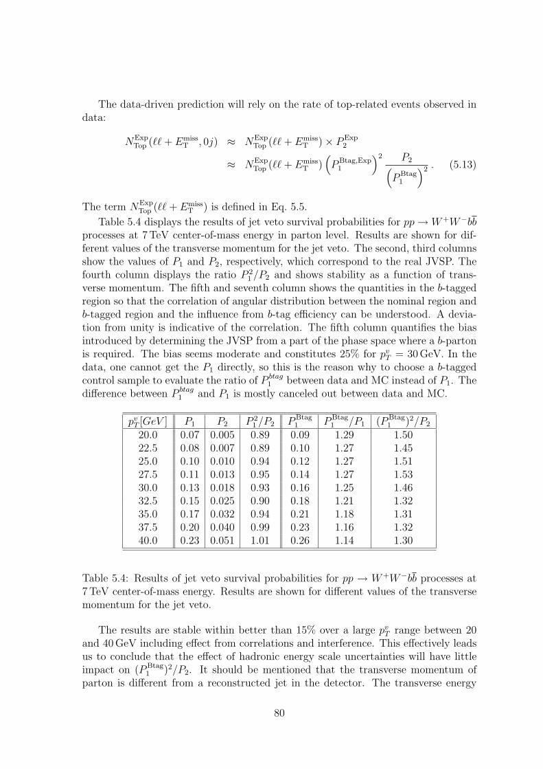
The data-driven prediction will rely on the rate of top-related events observed indata:
NExpTop (ℓℓ+ Emiss
T , 0j) ≈ NExpTop (ℓℓ+ Emiss
T ) × PExp2
≈ NExpTop (ℓℓ+ Emiss
T )(
PBtag,Exp1
)2 P2(
PBtag1
)2 . (5.13)
The term NExpTop (ℓℓ+ Emiss
T ) is defined in Eq. 5.5.
Table 5.4 displays the results of jet veto survival probabilities for pp→ W+W−bbprocesses at 7 TeV center-of-mass energy in parton level. Results are shown for dif-ferent values of the transverse momentum for the jet veto. The second, third columnsshow the values of P1 and P2, respectively, which correspond to the real JVSP. Thefourth column displays the ratio P 2
1 /P2 and shows stability as a function of trans-verse momentum. The fifth and seventh column shows the quantities in the b-taggedregion so that the correlation of angular distribution between the nominal region andb-tagged region and the influence from b-tag efficiency can be understood. A devia-tion from unity is indicative of the correlation. The fifth column quantifies the biasintroduced by determining the JVSP from a part of the phase space where a b-partonis required. The bias seems moderate and constitutes 25% for pv
T = 30 GeV. In thedata, one cannot get the P1 directly, so this is the reason why to choose a b-taggedcontrol sample to evaluate the ratio of P btag
1 between data and MC instead of P1. Thedifference between P btag
1 and P1 is mostly canceled out between data and MC.
pvT [GeV ] P1 P2 P 2
1 /P2 PBtag1 PBtag
1 /P1 (PBtag1 )2/P2
20.0 0.07 0.005 0.89 0.09 1.29 1.5022.5 0.08 0.007 0.89 0.10 1.27 1.4525.0 0.10 0.010 0.94 0.12 1.27 1.5127.5 0.11 0.013 0.95 0.14 1.27 1.5330.0 0.13 0.018 0.93 0.16 1.25 1.4632.5 0.15 0.025 0.90 0.18 1.21 1.3235.0 0.17 0.032 0.94 0.21 1.18 1.3137.5 0.20 0.040 0.99 0.23 1.16 1.3240.0 0.23 0.051 1.01 0.26 1.14 1.30
Table 5.4: Results of jet veto survival probabilities for pp → W+W−bb processes at7 TeV center-of-mass energy. Results are shown for different values of the transversemomentum for the jet veto.
The results are stable within better than 15% over a large pvT range between 20
and 40 GeV including effect from correlations and interference. This effectively leadsus to conclude that the effect of hadronic energy scale uncertainties will have littleimpact on (PBtag
1 )2/P2. It should be mentioned that the transverse momentum ofparton is different from a reconstructed jet in the detector. The transverse energy
80
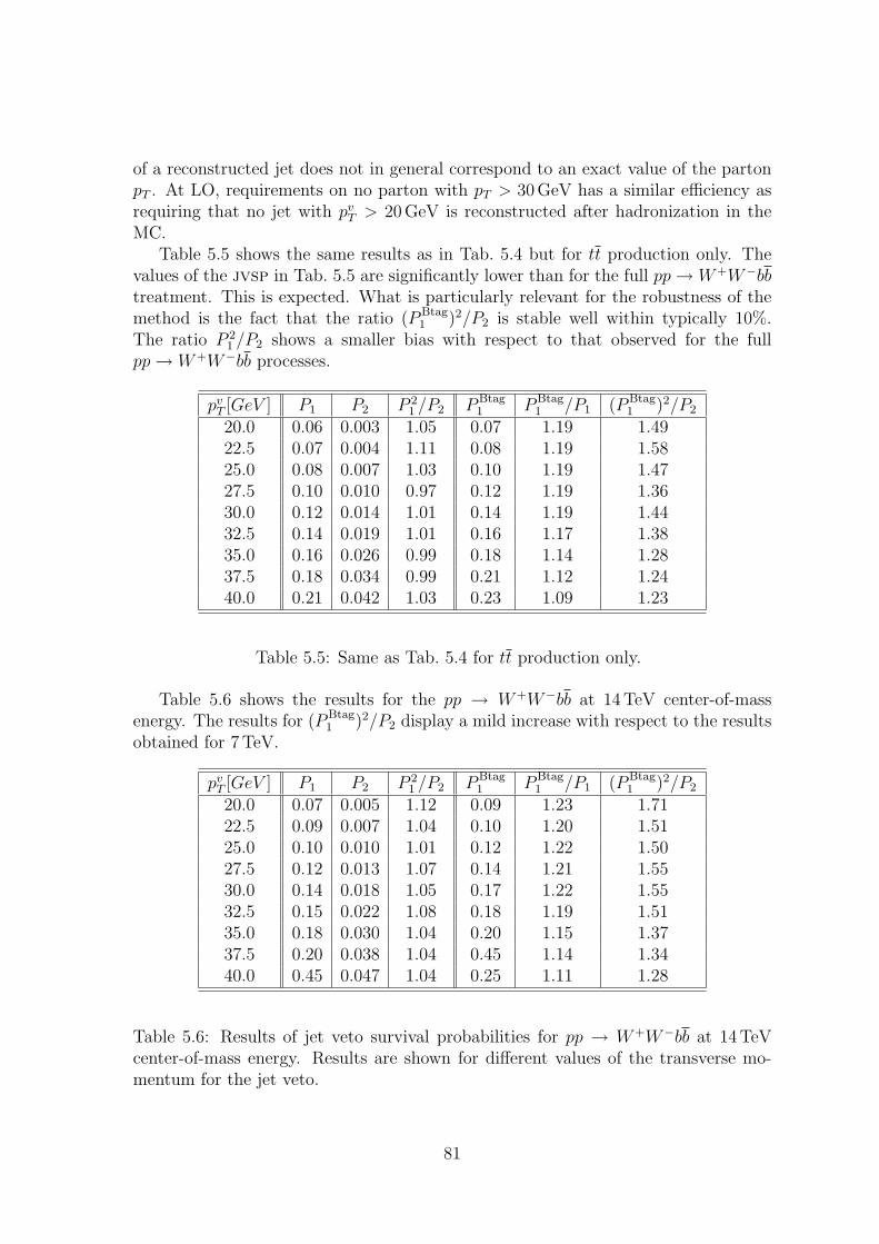
of a reconstructed jet does not in general correspond to an exact value of the partonpT . At LO, requirements on no parton with pT > 30GeV has a similar efficiency asrequiring that no jet with pv
T > 20GeV is reconstructed after hadronization in theMC.
Table 5.5 shows the same results as in Tab. 5.4 but for tt production only. Thevalues of the jvsp in Tab. 5.5 are significantly lower than for the full pp→ W+W−bbtreatment. This is expected. What is particularly relevant for the robustness of themethod is the fact that the ratio (PBtag
1 )2/P2 is stable well within typically 10%.The ratio P 2
1 /P2 shows a smaller bias with respect to that observed for the fullpp→ W+W−bb processes.
pvT [GeV ] P1 P2 P 2
1 /P2 PBtag1 PBtag
1 /P1 (PBtag1 )2/P2
20.0 0.06 0.003 1.05 0.07 1.19 1.4922.5 0.07 0.004 1.11 0.08 1.19 1.5825.0 0.08 0.007 1.03 0.10 1.19 1.4727.5 0.10 0.010 0.97 0.12 1.19 1.3630.0 0.12 0.014 1.01 0.14 1.19 1.4432.5 0.14 0.019 1.01 0.16 1.17 1.3835.0 0.16 0.026 0.99 0.18 1.14 1.2837.5 0.18 0.034 0.99 0.21 1.12 1.2440.0 0.21 0.042 1.03 0.23 1.09 1.23
Table 5.5: Same as Tab. 5.4 for tt production only.
Table 5.6 shows the results for the pp → W+W−bb at 14 TeV center-of-massenergy. The results for (PBtag
1 )2/P2 display a mild increase with respect to the resultsobtained for 7 TeV.
pvT [GeV ] P1 P2 P 2
1 /P2 PBtag1 PBtag
1 /P1 (PBtag1 )2/P2
20.0 0.07 0.005 1.12 0.09 1.23 1.7122.5 0.09 0.007 1.04 0.10 1.20 1.5125.0 0.10 0.010 1.01 0.12 1.22 1.5027.5 0.12 0.013 1.07 0.14 1.21 1.5530.0 0.14 0.018 1.05 0.17 1.22 1.5532.5 0.15 0.022 1.08 0.18 1.19 1.5135.0 0.18 0.030 1.04 0.20 1.15 1.3737.5 0.20 0.038 1.04 0.45 1.14 1.3440.0 0.45 0.047 1.04 0.25 1.11 1.28
Table 5.6: Results of jet veto survival probabilities for pp → W+W−bb at 14 TeVcenter-of-mass energy. Results are shown for different values of the transverse mo-mentum for the jet veto.
81
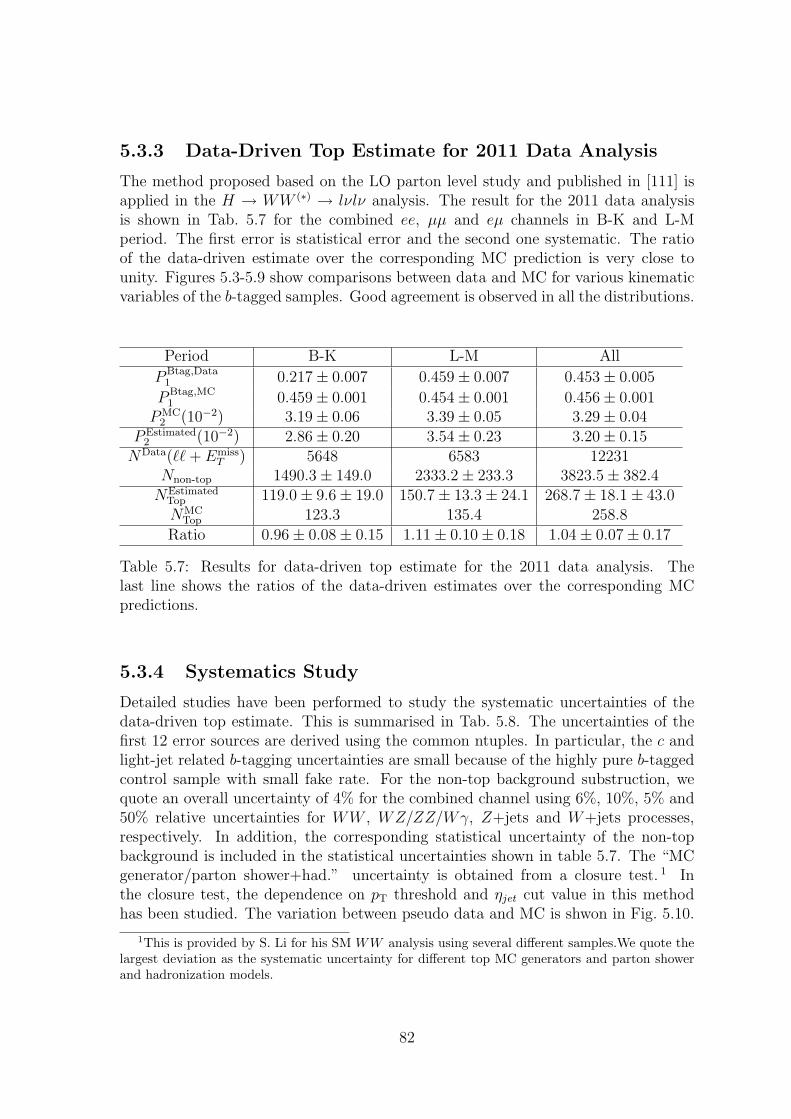
5.3.3 Data-Driven Top Estimate for 2011 Data Analysis
The method proposed based on the LO parton level study and published in [111] isapplied in the H → WW (∗) → lνlν analysis. The result for the 2011 data analysisis shown in Tab. 5.7 for the combined ee, µµ and eµ channels in B-K and L-Mperiod. The first error is statistical error and the second one systematic. The ratioof the data-driven estimate over the corresponding MC prediction is very close tounity. Figures 5.3-5.9 show comparisons between data and MC for various kinematicvariables of the b-tagged samples. Good agreement is observed in all the distributions.
Period B-K L-M All
PBtag,Data1 0.217 ± 0.007 0.459 ± 0.007 0.453 ± 0.005
PBtag,MC1 0.459 ± 0.001 0.454 ± 0.001 0.456 ± 0.001
PMC2 (10−2) 3.19 ± 0.06 3.39 ± 0.05 3.29 ± 0.04
PEstimated2 (10−2) 2.86 ± 0.20 3.54 ± 0.23 3.20 ± 0.15
NData(ℓℓ+ EmissT ) 5648 6583 12231
Nnon-top 1490.3 ± 149.0 2333.2 ± 233.3 3823.5 ± 382.4NEstimated
Top 119.0 ± 9.6 ± 19.0 150.7 ± 13.3 ± 24.1 268.7 ± 18.1 ± 43.0NMC
Top 123.3 135.4 258.8
Ratio 0.96 ± 0.08 ± 0.15 1.11 ± 0.10 ± 0.18 1.04 ± 0.07 ± 0.17
Table 5.7: Results for data-driven top estimate for the 2011 data analysis. Thelast line shows the ratios of the data-driven estimates over the corresponding MCpredictions.
5.3.4 Systematics Study
Detailed studies have been performed to study the systematic uncertainties of thedata-driven top estimate. This is summarised in Tab. 5.8. The uncertainties of thefirst 12 error sources are derived using the common ntuples. In particular, the c andlight-jet related b-tagging uncertainties are small because of the highly pure b-taggedcontrol sample with small fake rate. For the non-top background substruction, wequote an overall uncertainty of 4% for the combined channel using 6%, 10%, 5% and50% relative uncertainties for WW , WZ/ZZ/Wγ, Z+jets and W+jets processes,respectively. In addition, the corresponding statistical uncertainty of the non-topbackground is included in the statistical uncertainties shown in table 5.7. The “MCgenerator/parton shower+had.” uncertainty is obtained from a closure test. 1 Inthe closure test, the dependence on pT threshold and ηjet cut value in this methodhas been studied. The variation between pseudo data and MC is shwon in Fig. 5.10.
1This is provided by S. Li for his SM WW analysis using several different samples.We quote thelargest deviation as the systematic uncertainty for different top MC generators and parton showerand hadronization models.
82
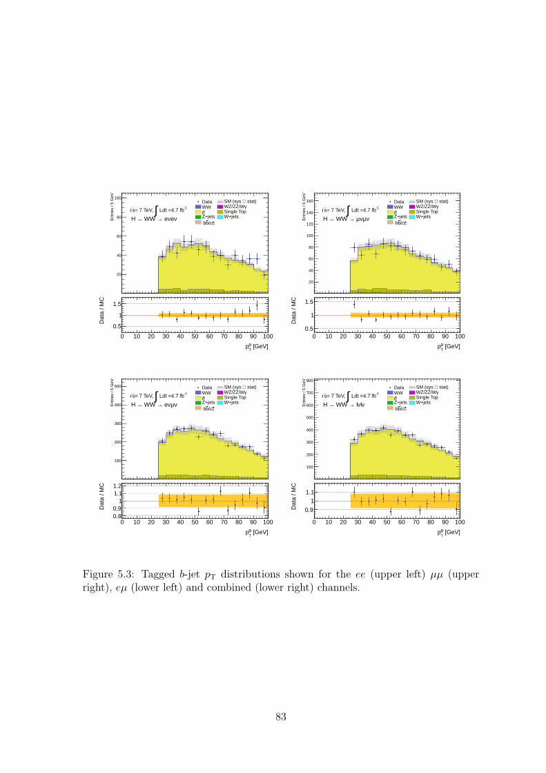
0 10 20 30 40 50 60 70 80 90 100
Ent
ries
/ 5 G
eV
20
40
60
80
100
-1 Ldt =4.7 fb∫= 7 TeV, s
νeν e→ WW → H
Data stat)⊕SM (sys WW γWZ/ZZ/Wtt Single TopZ+jets W+jets
c/cb b
0 10 20 30 40 50 60 70 80 90 100
Ent
ries
/ 5 G
eV
20
40
60
80
100
-1 Ldt =4.7 fb∫= 7 TeV, s
νeν e→ WW → H
Data stat)⊕SM (sys WW γWZ/ZZ/Wtt Single Top
Z+jets W+jetsc/cb b
[GeV]TBp
0 10 20 30 40 50 60 70 80 90 100
Dat
a / M
C
0.5
1
1.5
0 10 20 30 40 50 60 70 80 90 100
Ent
ries
/ 5 G
eV
20
40
60
80
100
120
140
160
-1 Ldt =4.7 fb∫= 7 TeV, s
νµνµ → WW → H
Data stat)⊕SM (sys WW γWZ/ZZ/Wtt Single TopZ+jets W+jets
c/cb b
0 10 20 30 40 50 60 70 80 90 100
Ent
ries
/ 5 G
eV
20
40
60
80
100
120
140
160
-1 Ldt =4.7 fb∫= 7 TeV, s
νµνµ → WW → H
Data stat)⊕SM (sys WW γWZ/ZZ/Wtt Single Top
Z+jets W+jetsc/cb b
[GeV]TBp
0 10 20 30 40 50 60 70 80 90 100
Dat
a / M
C
0.5
1
1.5
0 10 20 30 40 50 60 70 80 90 100
Ent
ries
/ 5 G
eV
100
200
300
400
500
-1 Ldt =4.7 fb∫= 7 TeV, s
νµν e→ WW → H
Data stat)⊕SM (sys WW γWZ/ZZ/Wtt Single TopZ+jets W+jets
c/cb b
0 10 20 30 40 50 60 70 80 90 100
Ent
ries
/ 5 G
eV
100
200
300
400
500
-1 Ldt =4.7 fb∫= 7 TeV, s
νµν e→ WW → H
Data stat)⊕SM (sys WW γWZ/ZZ/Wtt Single Top
Z+jets W+jetsc/cb b
[GeV]TBp
0 10 20 30 40 50 60 70 80 90 100
Dat
a / M
C
0.80.9
11.11.2
0 10 20 30 40 50 60 70 80 90 100
Ent
ries
/ 5 G
eV
100
200
300
400
500
600
700
800
-1 Ldt =4.7 fb∫= 7 TeV, s
νlν l→ WW → H
Data stat)⊕SM (sys WW γWZ/ZZ/Wtt Single TopZ+jets W+jets
c/cb b
0 10 20 30 40 50 60 70 80 90 100
Ent
ries
/ 5 G
eV
100
200
300
400
500
600
700
800
-1 Ldt =4.7 fb∫= 7 TeV, s
νlν l→ WW → H
Data stat)⊕SM (sys WW γWZ/ZZ/Wtt Single Top
Z+jets W+jetsc/cb b
[GeV]TBp
0 10 20 30 40 50 60 70 80 90 100
Dat
a / M
C
0.9
1
1.1
Figure 5.3: Tagged b-jet pT distributions shown for the ee (upper left) µµ (upperright), eµ (lower left) and combined (lower right) channels.
83
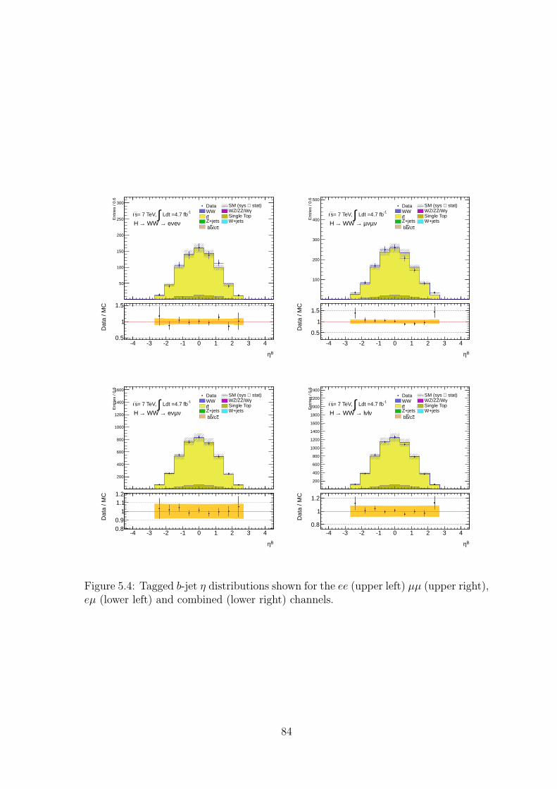
-4 -3 -2 -1 0 1 2 3 4
Ent
ries
/ 0.6
50
100
150
200
250
300
-1 Ldt =4.7 fb∫= 7 TeV, s
νeν e→ WW → H
Data stat)⊕SM (sys WW γWZ/ZZ/Wtt Single TopZ+jets W+jets
c/cb b
-4 -3 -2 -1 0 1 2 3 4
Ent
ries
/ 0.6
50
100
150
200
250
300
-1 Ldt =4.7 fb∫= 7 TeV, s
νeν e→ WW → H
Data stat)⊕SM (sys WW γWZ/ZZ/Wtt Single Top
Z+jets W+jetsc/cb b
Bη
-4 -3 -2 -1 0 1 2 3 4
Dat
a / M
C
0.5
1
1.5
-4 -3 -2 -1 0 1 2 3 4
Ent
ries
/ 0.6
100
200
300
400
500
-1 Ldt =4.7 fb∫= 7 TeV, s
νµνµ → WW → H
Data stat)⊕SM (sys WW γWZ/ZZ/Wtt Single TopZ+jets W+jets
c/cb b
-4 -3 -2 -1 0 1 2 3 4
Ent
ries
/ 0.6
100
200
300
400
500
-1 Ldt =4.7 fb∫= 7 TeV, s
νµνµ → WW → H
Data stat)⊕SM (sys WW γWZ/ZZ/Wtt Single Top
Z+jets W+jetsc/cb b
Bη
-4 -3 -2 -1 0 1 2 3 4
Dat
a / M
C
0.5
1
1.5
-4 -3 -2 -1 0 1 2 3 4
Ent
ries
/ 0.6
200
400
600
800
1000
1200
1400
1600
-1 Ldt =4.7 fb∫= 7 TeV, s
νµν e→ WW → H
Data stat)⊕SM (sys WW γWZ/ZZ/Wtt Single TopZ+jets W+jets
c/cb b
-4 -3 -2 -1 0 1 2 3 4
Ent
ries
/ 0.6
200
400
600
800
1000
1200
1400
1600
-1 Ldt =4.7 fb∫= 7 TeV, s
νµν e→ WW → H
Data stat)⊕SM (sys WW γWZ/ZZ/Wtt Single Top
Z+jets W+jetsc/cb b
Bη
-4 -3 -2 -1 0 1 2 3 4
Dat
a / M
C
0.80.9
11.11.2
-4 -3 -2 -1 0 1 2 3 4
Ent
ries
/ 0.6
200
400
600
800
1000
1200
1400
1600
1800
2000
2200
2400
-1 Ldt =4.7 fb∫= 7 TeV, s
νlν l→ WW → H
Data stat)⊕SM (sys WW γWZ/ZZ/Wtt Single TopZ+jets W+jets
c/cb b
-4 -3 -2 -1 0 1 2 3 4
Ent
ries
/ 0.6
200
400
600
800
1000
1200
1400
1600
1800
2000
2200
2400
-1 Ldt =4.7 fb∫= 7 TeV, s
νlν l→ WW → H
Data stat)⊕SM (sys WW γWZ/ZZ/Wtt Single Top
Z+jets W+jetsc/cb b
Bη
-4 -3 -2 -1 0 1 2 3 4
Dat
a / M
C
0.8
1
1.2
Figure 5.4: Tagged b-jet η distributions shown for the ee (upper left) µµ (upper right),eµ (lower left) and combined (lower right) channels.
84
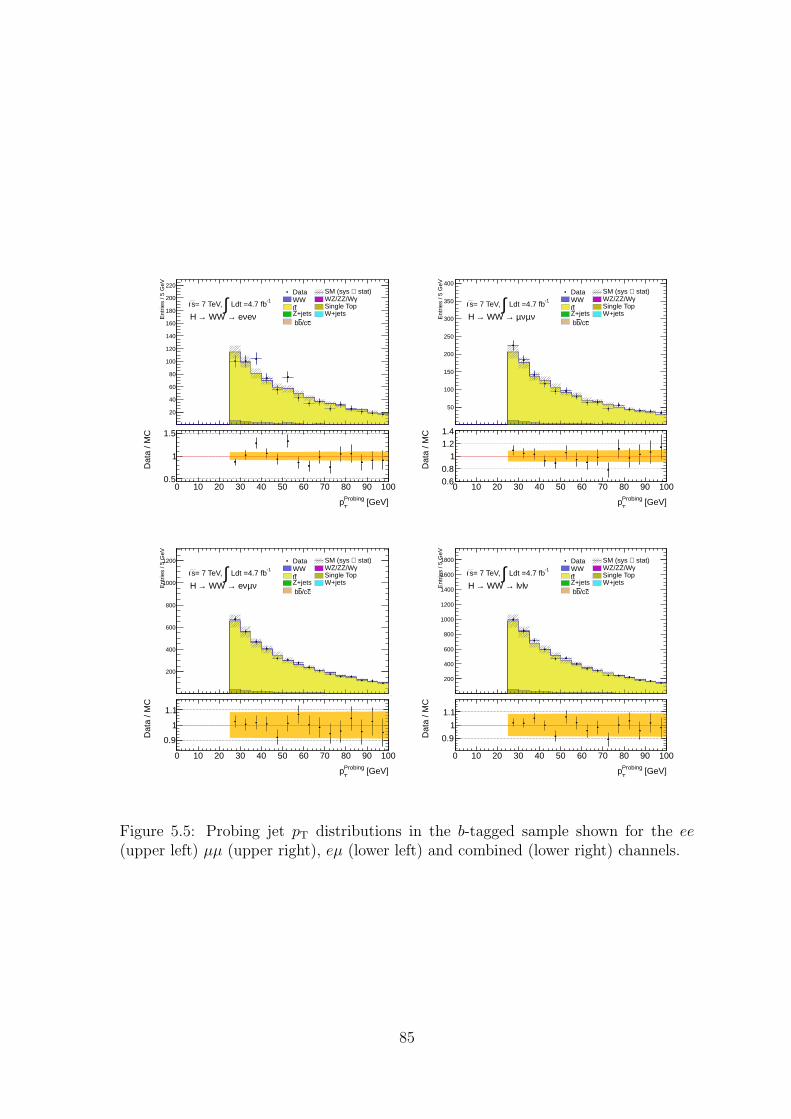
0 10 20 30 40 50 60 70 80 90 100
Ent
ries
/ 5 G
eV
20
40
60
80
100
120
140
160
180
200
220
-1 Ldt =4.7 fb∫= 7 TeV, s
νeν e→ WW → H
Data stat)⊕SM (sys WW γWZ/ZZ/Wtt Single TopZ+jets W+jets
c/cb b
0 10 20 30 40 50 60 70 80 90 100
Ent
ries
/ 5 G
eV
20
40
60
80
100
120
140
160
180
200
220
-1 Ldt =4.7 fb∫= 7 TeV, s
νeν e→ WW → H
Data stat)⊕SM (sys WW γWZ/ZZ/Wtt Single Top
Z+jets W+jetsc/cb b
[GeV]T
Probingp
0 10 20 30 40 50 60 70 80 90 100
Dat
a / M
C
0.5
1
1.5
0 10 20 30 40 50 60 70 80 90 100
Ent
ries
/ 5 G
eV
50
100
150
200
250
300
350
400
-1 Ldt =4.7 fb∫= 7 TeV, s
νµνµ → WW → H
Data stat)⊕SM (sys WW γWZ/ZZ/Wtt Single TopZ+jets W+jets
c/cb b
0 10 20 30 40 50 60 70 80 90 100
Ent
ries
/ 5 G
eV
50
100
150
200
250
300
350
400
-1 Ldt =4.7 fb∫= 7 TeV, s
νµνµ → WW → H
Data stat)⊕SM (sys WW γWZ/ZZ/Wtt Single Top
Z+jets W+jetsc/cb b
[GeV]T
Probingp
0 10 20 30 40 50 60 70 80 90 100
Dat
a / M
C
0.6
0.8
1
1.2
1.4
0 10 20 30 40 50 60 70 80 90 100
Ent
ries
/ 5 G
eV
200
400
600
800
1000
1200-1
Ldt =4.7 fb∫= 7 TeV, s
νµν e→ WW → H
Data stat)⊕SM (sys WW γWZ/ZZ/Wtt Single TopZ+jets W+jets
c/cb b
0 10 20 30 40 50 60 70 80 90 100
Ent
ries
/ 5 G
eV
200
400
600
800
1000
1200-1 Ldt =4.7 fb∫= 7 TeV, s
νµν e→ WW → H
Data stat)⊕SM (sys WW γWZ/ZZ/Wtt Single Top
Z+jets W+jetsc/cb b
[GeV]T
Probingp
0 10 20 30 40 50 60 70 80 90 100
Dat
a / M
C
0.9
1
1.1
0 10 20 30 40 50 60 70 80 90 100
Ent
ries
/ 5 G
eV
200
400
600
800
1000
1200
1400
1600
1800
-1 Ldt =4.7 fb∫= 7 TeV, s
νlν l→ WW → H
Data stat)⊕SM (sys WW γWZ/ZZ/Wtt Single TopZ+jets W+jets
c/cb b
0 10 20 30 40 50 60 70 80 90 100
Ent
ries
/ 5 G
eV
200
400
600
800
1000
1200
1400
1600
1800
-1 Ldt =4.7 fb∫= 7 TeV, s
νlν l→ WW → H
Data stat)⊕SM (sys WW γWZ/ZZ/Wtt Single Top
Z+jets W+jetsc/cb b
[GeV]T
Probingp
0 10 20 30 40 50 60 70 80 90 100
Dat
a / M
C
0.9
1
1.1
Figure 5.5: Probing jet pT distributions in the b-tagged sample shown for the ee(upper left) µµ (upper right), eµ (lower left) and combined (lower right) channels.
85
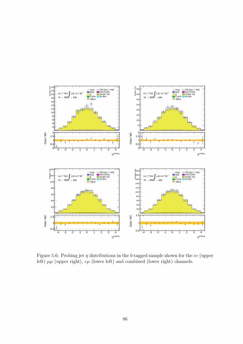
-4 -3 -2 -1 0 1 2 3 4
Ent
ries
/ 0.6
20
40
60
80
100
120
140
160
180
200
220
240
-1 Ldt =4.7 fb∫= 7 TeV, s
νlν l→ WW → H
Data stat)⊕SM (sys WW γWZ/ZZ/Wtt Single TopZ+jets W+jets
c/cb b
-4 -3 -2 -1 0 1 2 3 4
Ent
ries
/ 0.6
20
40
60
80
100
120
140
160
180
200
220
240
-1 Ldt =4.7 fb∫= 7 TeV, s
νlν l→ WW → H
Data stat)⊕SM (sys WW γWZ/ZZ/Wtt Single Top
Z+jets W+jetsc/cb b
probingη
-4 -3 -2 -1 0 1 2 3 4
Dat
a / M
C
0
0.5
1
1.5
2
-4 -3 -2 -1 0 1 2 3 4
Ent
ries
/ 0.6
50
100
150
200
250
300
350
400
-1 Ldt =4.7 fb∫= 7 TeV, s
νlν l→ WW → H
Data stat)⊕SM (sys WW γWZ/ZZ/Wtt Single TopZ+jets W+jets
c/cb b
-4 -3 -2 -1 0 1 2 3 4
Ent
ries
/ 0.6
50
100
150
200
250
300
350
400
-1 Ldt =4.7 fb∫= 7 TeV, s
νlν l→ WW → H
Data stat)⊕SM (sys WW γWZ/ZZ/Wtt Single Top
Z+jets W+jetsc/cb b
probingη
-4 -3 -2 -1 0 1 2 3 4
Dat
a / M
C
0
0.5
1
1.5
2
-4 -3 -2 -1 0 1 2 3 4
Ent
ries
/ 0.6
200
400
600
800
1000
1200
1400
-1 Ldt =4.7 fb∫= 7 TeV, s
νlν l→ WW → H
Data stat)⊕SM (sys WW γWZ/ZZ/Wtt Single TopZ+jets W+jets
c/cb b
-4 -3 -2 -1 0 1 2 3 4
Ent
ries
/ 0.6
200
400
600
800
1000
1200
1400
-1 Ldt =4.7 fb∫= 7 TeV, s
νlν l→ WW → H
Data stat)⊕SM (sys WW γWZ/ZZ/Wtt Single Top
Z+jets W+jetsc/cb b
probingη
-4 -3 -2 -1 0 1 2 3 4
Dat
a / M
C
0.5
1
1.5
-4 -3 -2 -1 0 1 2 3 4
Ent
ries
/ 0.6
200
400
600
800
1000
1200
1400
1600
1800
2000
-1 Ldt =4.7 fb∫= 7 TeV, s
νlν l→ WW → H
Data stat)⊕SM (sys WW γWZ/ZZ/Wtt Single TopZ+jets W+jets
c/cb b
-4 -3 -2 -1 0 1 2 3 4
Ent
ries
/ 0.6
200
400
600
800
1000
1200
1400
1600
1800
2000
-1 Ldt =4.7 fb∫= 7 TeV, s
νlν l→ WW → H
Data stat)⊕SM (sys WW γWZ/ZZ/Wtt Single Top
Z+jets W+jetsc/cb b
probingη
-4 -3 -2 -1 0 1 2 3 4
Dat
a / M
C
0.5
1
1.5
Figure 5.6: Probing jet η distributions in the b-tagged sample shown for the ee (upperleft) µµ (upper right), eµ (lower left) and combined (lower right) channels.
86
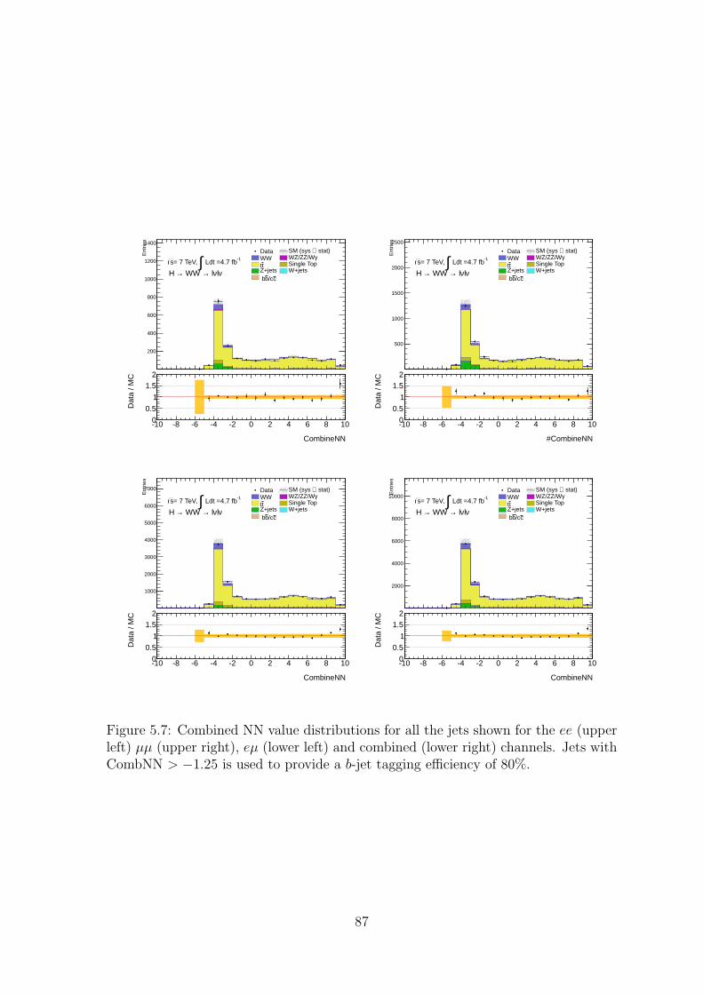
-10 -8 -6 -4 -2 0 2 4 6 8 10
Ent
ries
200
400
600
800
1000
1200
1400
-1 Ldt =4.7 fb∫= 7 TeV, s
νlν l→ WW → H
Data stat)⊕SM (sys WW γWZ/ZZ/Wtt Single TopZ+jets W+jets
c/cb b
-10 -8 -6 -4 -2 0 2 4 6 8 10
Ent
ries
200
400
600
800
1000
1200
1400
-1 Ldt =4.7 fb∫= 7 TeV, s
νlν l→ WW → H
Data stat)⊕SM (sys WW γWZ/ZZ/Wtt Single Top
Z+jets W+jetsc/cb b
CombineNN
-10 -8 -6 -4 -2 0 2 4 6 8 10
Dat
a / M
C
0
0.5
1
1.5
2
-10 -8 -6 -4 -2 0 2 4 6 8 10
Ent
ries
500
1000
1500
2000
2500
-1 Ldt =4.7 fb∫= 7 TeV, s
νlν l→ WW → H
Data stat)⊕SM (sys WW γWZ/ZZ/Wtt Single TopZ+jets W+jets
c/cb b
-10 -8 -6 -4 -2 0 2 4 6 8 10
Ent
ries
500
1000
1500
2000
2500
-1 Ldt =4.7 fb∫= 7 TeV, s
νlν l→ WW → H
Data stat)⊕SM (sys WW γWZ/ZZ/Wtt Single Top
Z+jets W+jetsc/cb b
#CombineNN
-10 -8 -6 -4 -2 0 2 4 6 8 10
Dat
a / M
C
0
0.5
1
1.5
2
-10 -8 -6 -4 -2 0 2 4 6 8 10
Ent
ries
1000
2000
3000
4000
5000
6000
7000
-1 Ldt =4.7 fb∫= 7 TeV, s
νlν l→ WW → H
Data stat)⊕SM (sys WW γWZ/ZZ/Wtt Single TopZ+jets W+jets
c/cb b
-10 -8 -6 -4 -2 0 2 4 6 8 10
Ent
ries
1000
2000
3000
4000
5000
6000
7000
-1 Ldt =4.7 fb∫= 7 TeV, s
νlν l→ WW → H
Data stat)⊕SM (sys WW γWZ/ZZ/Wtt Single Top
Z+jets W+jetsc/cb b
CombineNN
-10 -8 -6 -4 -2 0 2 4 6 8 10
Dat
a / M
C
0
0.5
1
1.5
2
-10 -8 -6 -4 -2 0 2 4 6 8 10
Ent
ries
2000
4000
6000
8000
10000 -1 Ldt =4.7 fb∫= 7 TeV, s
νlν l→ WW → H
Data stat)⊕SM (sys WW γWZ/ZZ/Wtt Single TopZ+jets W+jets
c/cb b
-10 -8 -6 -4 -2 0 2 4 6 8 10
Ent
ries
2000
4000
6000
8000
10000 -1 Ldt =4.7 fb∫= 7 TeV, s
νlν l→ WW → H
Data stat)⊕SM (sys WW γWZ/ZZ/Wtt Single Top
Z+jets W+jetsc/cb b
CombineNN
-10 -8 -6 -4 -2 0 2 4 6 8 10
Dat
a / M
C
0
0.5
1
1.5
2
Figure 5.7: Combined NN value distributions for all the jets shown for the ee (upperleft) µµ (upper right), eµ (lower left) and combined (lower right) channels. Jets withCombNN > −1.25 is used to provide a b-jet tagging efficiency of 80%.
87
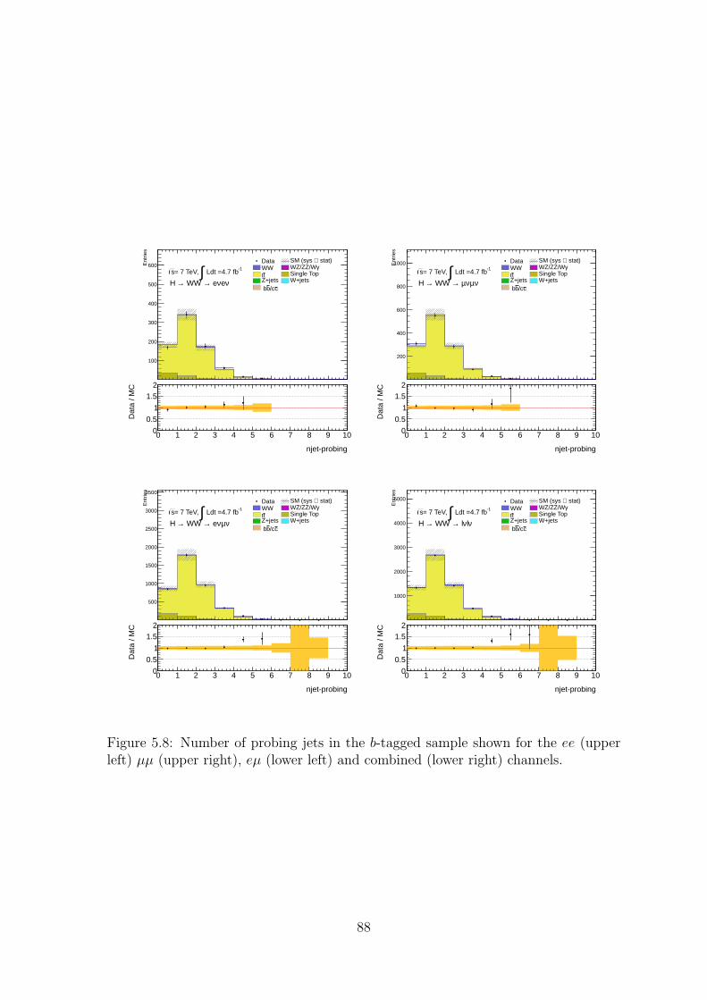
0 1 2 3 4 5 6 7 8 9 10
Ent
ries
100
200
300
400
500
600-1
Ldt =4.7 fb∫= 7 TeV, s
νeν e→ WW → H
Data stat)⊕SM (sys WW γWZ/ZZ/Wtt Single TopZ+jets W+jets
c/cb b
0 1 2 3 4 5 6 7 8 9 10
Ent
ries
100
200
300
400
500
600-1 Ldt =4.7 fb∫= 7 TeV, s
νeν e→ WW → H
Data stat)⊕SM (sys WW γWZ/ZZ/Wtt Single Top
Z+jets W+jetsc/cb b
njet-probing
0 1 2 3 4 5 6 7 8 9 10
Dat
a / M
C
0
0.5
1
1.5
2
0 1 2 3 4 5 6 7 8 9 10
Ent
ries
200
400
600
800
1000-1
Ldt =4.7 fb∫= 7 TeV, s
νµνµ → WW → H
Data stat)⊕SM (sys WW γWZ/ZZ/Wtt Single TopZ+jets W+jets
c/cb b
0 1 2 3 4 5 6 7 8 9 10
Ent
ries
200
400
600
800
1000-1 Ldt =4.7 fb∫= 7 TeV, s
νµνµ → WW → H
Data stat)⊕SM (sys WW γWZ/ZZ/Wtt Single Top
Z+jets W+jetsc/cb b
njet-probing
0 1 2 3 4 5 6 7 8 9 10
Dat
a / M
C
0
0.5
1
1.5
2
0 1 2 3 4 5 6 7 8 9 10
Ent
ries
500
1000
1500
2000
2500
3000
3500
-1 Ldt =4.7 fb∫= 7 TeV, s
νµν e→ WW → H
Data stat)⊕SM (sys WW γWZ/ZZ/Wtt Single TopZ+jets W+jets
c/cb b
0 1 2 3 4 5 6 7 8 9 10
Ent
ries
500
1000
1500
2000
2500
3000
3500
-1 Ldt =4.7 fb∫= 7 TeV, s
νµν e→ WW → H
Data stat)⊕SM (sys WW γWZ/ZZ/Wtt Single Top
Z+jets W+jetsc/cb b
njet-probing
0 1 2 3 4 5 6 7 8 9 10
Dat
a / M
C
0
0.5
1
1.5
2
0 1 2 3 4 5 6 7 8 9 10
Ent
ries
1000
2000
3000
4000
5000
-1 Ldt =4.7 fb∫= 7 TeV, s
νlν l→ WW → H
Data stat)⊕SM (sys WW γWZ/ZZ/Wtt Single TopZ+jets W+jets
c/cb b
0 1 2 3 4 5 6 7 8 9 10
Ent
ries
1000
2000
3000
4000
5000
-1 Ldt =4.7 fb∫= 7 TeV, s
νlν l→ WW → H
Data stat)⊕SM (sys WW γWZ/ZZ/Wtt Single Top
Z+jets W+jetsc/cb b
njet-probing
0 1 2 3 4 5 6 7 8 9 10
Dat
a / M
C
0
0.5
1
1.5
2
Figure 5.8: Number of probing jets in the b-tagged sample shown for the ee (upperleft) µµ (upper right), eµ (lower left) and combined (lower right) channels.
88
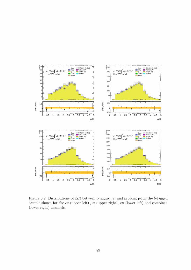
0 0.5 1 1.5 2 2.5 3 3.5 4 4.5 5
Ent
ries
20
40
60
80
100
120
140
160
180
200
-1 Ldt =4.7 fb∫= 7 TeV, s
νlν l→ WW → H
Data stat)⊕SM (sys WW γWZ/ZZ/Wtt Single TopZ+jets W+jets
c/cb b
0 0.5 1 1.5 2 2.5 3 3.5 4 4.5 5
Ent
ries
20
40
60
80
100
120
140
160
180
200
-1 Ldt =4.7 fb∫= 7 TeV, s
νlν l→ WW → H
Data stat)⊕SM (sys WW γWZ/ZZ/Wtt Single Top
Z+jets W+jetsc/cb b
R∆
0 0.5 1 1.5 2 2.5 3 3.5 4 4.5 5
Dat
a / M
C
0.5
1
1.5
0 0.5 1 1.5 2 2.5 3 3.5 4 4.5 5
Ent
ries
50
100
150
200
250
300
350
-1 Ldt =4.7 fb∫= 7 TeV, s
νlν l→ WW → H
Data stat)⊕SM (sys WW γWZ/ZZ/Wtt Single TopZ+jets W+jets
c/cb b
0 0.5 1 1.5 2 2.5 3 3.5 4 4.5 5
Ent
ries
50
100
150
200
250
300
350
-1 Ldt =4.7 fb∫= 7 TeV, s
νlν l→ WW → H
Data stat)⊕SM (sys WW γWZ/ZZ/Wtt Single Top
Z+jets W+jetsc/cb b
R∆
0 0.5 1 1.5 2 2.5 3 3.5 4 4.5 5
Dat
a / M
C
0.5
1
1.5
0 0.5 1 1.5 2 2.5 3 3.5 4 4.5 5
Ent
ries
200
400
600
800
1000
1200
-1 Ldt =4.7 fb∫= 7 TeV, s
νlν l→ WW → H
Data stat)⊕SM (sys WW γWZ/ZZ/Wtt Single TopZ+jets W+jets
c/cb b
0 0.5 1 1.5 2 2.5 3 3.5 4 4.5 5
Ent
ries
200
400
600
800
1000
1200
-1 Ldt =4.7 fb∫= 7 TeV, s
νlν l→ WW → H
Data stat)⊕SM (sys WW γWZ/ZZ/Wtt Single Top
Z+jets W+jetsc/cb b
R∆
0 0.5 1 1.5 2 2.5 3 3.5 4 4.5 5
Dat
a / M
C
0.8
1
1.2
0 0.5 1 1.5 2 2.5 3 3.5 4 4.5 5
Ent
ries
200
400
600
800
1000
1200
1400
1600
1800
-1 Ldt =4.7 fb∫= 7 TeV, s
νlν l→ WW → H
Data stat)⊕SM (sys WW γWZ/ZZ/Wtt Single TopZ+jets W+jets
c/cb b
0 0.5 1 1.5 2 2.5 3 3.5 4 4.5 5
Ent
ries
200
400
600
800
1000
1200
1400
1600
1800
-1 Ldt =4.7 fb∫= 7 TeV, s
νlν l→ WW → H
Data stat)⊕SM (sys WW γWZ/ZZ/Wtt Single Top
Z+jets W+jetsc/cb b
#R∆
0 0.5 1 1.5 2 2.5 3 3.5 4 4.5 5
Dat
a / M
C
0.8
1
1.2
Figure 5.9: Distributions of ∆R between b-tagged jet and probing jet in the b-taggedsample shown for the ee (upper left) µµ (upper right), eµ (lower left) and combined(lower right) channels.
89
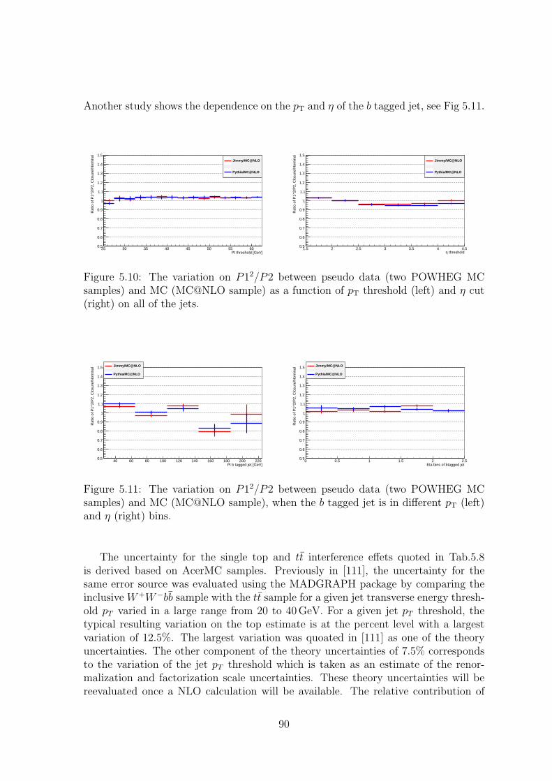
Another study shows the dependence on the pT and η of the b tagged jet, see Fig 5.11.
Pt threshold [GeV]25 30 35 40 45 50 55 60
Rat
io o
f P1^
2/P
2, C
losu
re/N
omin
al
0.5
0.6
0.7
0.8
0.9
1
1.1
1.2
1.3
1.4
1.5Jimmy/MC@NLO
Pythia/MC@NLO
thresholdη1.5 2 2.5 3 3.5 4 4.5
Rat
io o
f P1^
2/P
2, C
losu
re/N
omin
al
0.5
0.6
0.7
0.8
0.9
1
1.1
1.2
1.3
1.4
1.5Jimmy/MC@NLO
Pythia/MC@NLO
Figure 5.10: The variation on P12/P2 between pseudo data (two POWHEG MCsamples) and MC (MC@NLO sample) as a function of pT threshold (left) and η cut(right) on all of the jets.
Pt b tagged jet [GeV]40 60 80 100 120 140 160 180 200 220
Rat
io o
f P1^
2/P
2, C
losu
re/N
omin
al
0.5
0.6
0.7
0.8
0.9
1
1.1
1.2
1.3
1.4
1.5 Jimmy/MC@NLO
Pythia/MC@NLO
Eta bins of btagged jet0 0.5 1 1.5 2 2.5
Rat
io o
f P1^
2/P
2, C
losu
re/N
omin
al
0.5
0.6
0.7
0.8
0.9
1
1.1
1.2
1.3
1.4
1.5 Jimmy/MC@NLO
Pythia/MC@NLO
Figure 5.11: The variation on P12/P2 between pseudo data (two POWHEG MCsamples) and MC (MC@NLO sample), when the b tagged jet is in different pT (left)and η (right) bins.
The uncertainty for the single top and tt interference effets quoted in Tab.5.8is derived based on AcerMC samples. Previously in [111], the uncertainty for thesame error source was evaluated using the MADGRAPH package by comparing theinclusive W+W−bb sample with the tt sample for a given jet transverse energy thresh-old pT varied in a large range from 20 to 40GeV. For a given jet pT threshold, thetypical resulting variation on the top estimate is at the percent level with a largestvariation of 12.5%. The largest variation was quoated in [111] as one of the theoryuncertainties. The other component of the theory uncertainties of 7.5% correspondsto the variation of the jet pT threshold which is taken as an estimate of the renor-malization and factorization scale uncertainties. These theory uncertainties will bereevaluated once a NLO calculation will be available. The relative contribution of
90
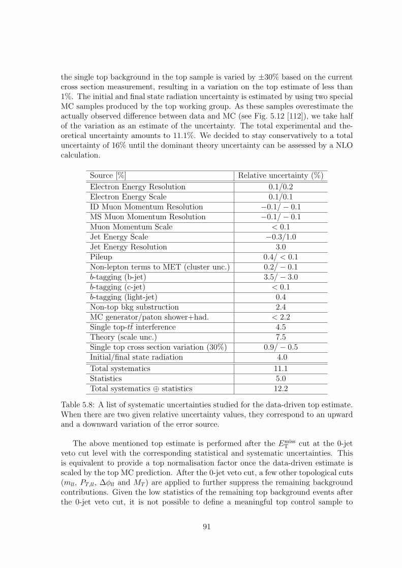
the single top background in the top sample is varied by ±30% based on the currentcross section measurement, resulting in a variation on the top estimate of less than1%. The initial and final state radiation uncertainty is estimated by using two specialMC samples produced by the top working group. As these samples overestimate theactually observed difference between data and MC (see Fig. 5.12 [112]), we take halfof the variation as an estimate of the uncertainty. The total experimental and the-oretical uncertainty amounts to 11.1%. We decided to stay conservatively to a totaluncertainty of 16% until the dominant theory uncertainty can be assessed by a NLOcalculation.
Source [%] Relative uncertainty (%)
Electron Energy Resolution 0.1/0.2Electron Energy Scale 0.1/0.1ID Muon Momentum Resolution −0.1/− 0.1MS Muon Momentum Resolution −0.1/− 0.1Muon Momentum Scale < 0.1Jet Energy Scale −0.3/1.0Jet Energy Resolution 3.0Pileup 0.4/ < 0.1Non-lepton terms to MET (cluster unc.) 0.2/− 0.1b-tagging (b-jet) 3.5/− 3.0b-tagging (c-jet) < 0.1b-tagging (light-jet) 0.4Non-top bkg substruction 2.4MC generator/paton shower+had. < 2.2Single top-tt interference 4.5Theory (scale unc.) 7.5Single top cross section variation (30%) 0.9/− 0.5Initial/final state radiation 4.0
Total systematics 11.1Statistics 5.0Total systematics ⊕ statistics 12.2
Table 5.8: A list of systematic uncertainties studied for the data-driven top estimate.When there are two given relative uncertainty values, they correspond to an upwardand a downward variation of the error source.
The above mentioned top estimate is performed after the EmissT cut at the 0-jet
veto cut level with the corresponding statistical and systematic uncertainties. Thisis equivalent to provide a top normalisation factor once the data-driven estimate isscaled by the top MC prediction. After the 0-jet veto cut, a few other topological cuts(mll, PT,ll, ∆φll and MT ) are applied to further suppress the remaining backgroundcontributions. Given the low statistics of the remaining top background events afterthe 0-jet veto cut, it is not possible to define a meaningful top control sample to
91
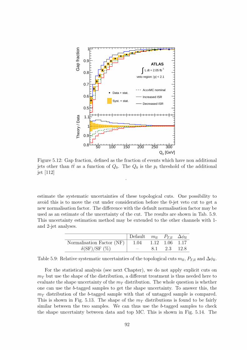
[GeV]0Q50 100 150 200 250 300
The
ory
/ Dat
a
0.8
0.9
1
1.1 50 100 150 200 250 300
Gap
frac
tion
0.5
0.6
0.7
0.8
0.9
1
Data + stat.
Syst. + stat.
MC nominalCERA
Increased ISR
Decreased ISR
veto region: |y| < 2.1
-1 L dt = 2.05 fb∫
ATLAS
Figure 5.12: Gap fraction, defined as the fraction of events which have non additionaljets other than tt as a function of Q0. The Q0 is the pt threshold of the additionaljet [112]
.
estimate the systematic uncertainties of these topological cuts. One possibility toavoid this is to move the cut under consideration before the 0-jet veto cut to get anew normalisation factor. The difference with the default normalisation factor may beused as an estimate of the uncertainty of the cut. The results are shown in Tab. 5.9.This uncertainty estimation method may be extended to the other channels with 1-and 2-jet analyses.
Default mll PT,ll ∆φll
Normalisation Factor (NF) 1.04 1.12 1.06 1.17δ(SF)/SF (%) – 8.1 2.3 12.8
Table 5.9: Relative systematic uncertainties of the topological cuts mll, PT,ll and ∆φll.
For the statistical analysis (see next Chapter), we do not apply explicit cuts onmT but use the shape of the distribution, a different treatment is thus needed here toevaluate the shape uncertainty of the mT distribution. The whole question is whetherone can use the b-tagged samples to get the shape uncertainty. To answer this, themT distribution of the b-tagged sample with that of untagged sample is compared.This is shown in Fig. 5.13. The shape of the mT distributions is found to be fairlysimilar between the two samples. We can thus use the b-tagged samples to checkthe shape uncertainty between data and top MC. This is shown in Fig. 5.14. The
92
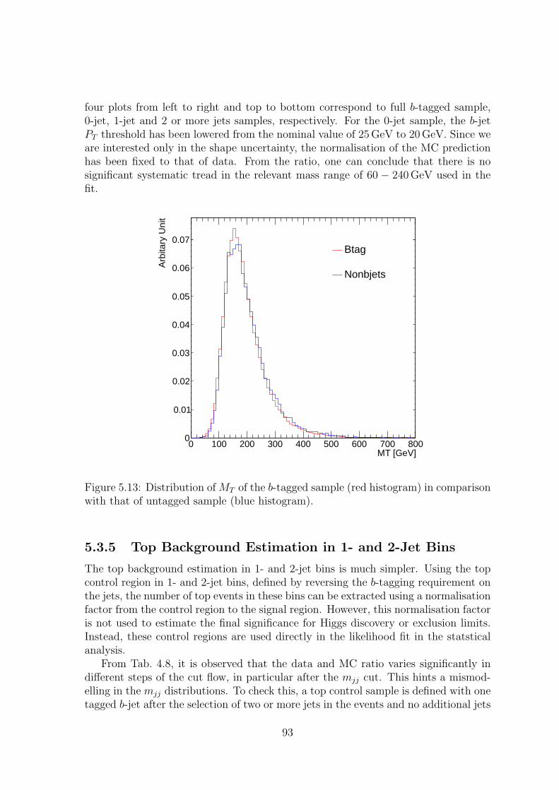
four plots from left to right and top to bottom correspond to full b-tagged sample,0-jet, 1-jet and 2 or more jets samples, respectively. For the 0-jet sample, the b-jetPT threshold has been lowered from the nominal value of 25 GeV to 20GeV. Since weare interested only in the shape uncertainty, the normalisation of the MC predictionhas been fixed to that of data. From the ratio, one can conclude that there is nosignificant systematic tread in the relevant mass range of 60 − 240 GeV used in thefit.
MT [GeV]0 100 200 300 400 500 600 700 800
Arb
itary
Uni
t
0
0.01
0.02
0.03
0.04
0.05
0.06
0.07Btag
Nonbjets
Figure 5.13: Distribution of MT of the b-tagged sample (red histogram) in comparisonwith that of untagged sample (blue histogram).
5.3.5 Top Background Estimation in 1- and 2-Jet Bins
The top background estimation in 1- and 2-jet bins is much simpler. Using the topcontrol region in 1- and 2-jet bins, defined by reversing the b-tagging requirement onthe jets, the number of top events in these bins can be extracted using a normalisationfactor from the control region to the signal region. However, this normalisation factoris not used to estimate the final significance for Higgs discovery or exclusion limits.Instead, these control regions are used directly in the likelihood fit in the statsticalanalysis.
From Tab. 4.8, it is observed that the data and MC ratio varies significantly indifferent steps of the cut flow, in particular after the mjj cut. This hints a mismod-elling in the mjj distributions. To check this, a top control sample is defined with onetagged b-jet after the selection of two or more jets in the events and no additional jets
93
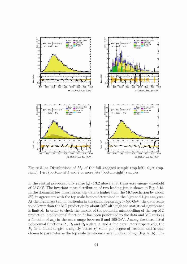
50 100 150 200 250 300 350 400 450
Ent
ries
/ 10
GeV
100
200
300
400
500
600
700
800
900
-1 Ldt =4.7 fb∫= 7 TeV, s
νlν l→ WW → H
Data stat)⊕SM (sys WW γWZ/ZZ/Wtt Single Top
Z+jets W+jetsc/cb b
50 100 150 200 250 300 350 400 450
Ent
ries
/ 10
GeV
100
200
300
400
500
600
700
800
900
-1 Ldt =4.7 fb∫= 7 TeV, s
νlν l→ WW → H
Data stat)⊕SM (sys WW γWZ/ZZ/Wtt Single Top
Z+jets W+jetsc/cb b
-25GeV_bjet_all [GeV]TM
50 100 150 200 250 300 350 400 450
Dat
a / M
C
0
0.5
1
1.5
2
50 100 150 200 250 300 350 400 450
Ent
ries
/ 10
GeV
2
4
6
8
10
12
14
-1 Ldt =4.7 fb∫= 7 TeV, s
νlν l→ WW → H
Data stat)⊕SM (sys WW γWZ/ZZ/Wtt Single Top
Z+jets W+jetsc/cb b
50 100 150 200 250 300 350 400 450
Ent
ries
/ 10
GeV
2
4
6
8
10
12
14
-1 Ldt =4.7 fb∫= 7 TeV, s
νlν l→ WW → H
Data stat)⊕SM (sys WW γWZ/ZZ/Wtt Single Top
Z+jets W+jetsc/cb b
-20GeV_bjet_0jet [GeV]TM
50 100 150 200 250 300 350 400 450
Dat
a / M
C
0
0.5
1
1.5
2
50 100 150 200 250 300 350 400 450
Ent
ries
/ 10
GeV
20
40
60
80
100
120
140
160
180
-1 Ldt =4.7 fb∫= 7 TeV, s
νlν l→ WW → H
Data stat)⊕SM (sys WW γWZ/ZZ/Wtt Single Top
Z+jets W+jetsc/cb b
50 100 150 200 250 300 350 400 450
Ent
ries
/ 10
GeV
20
40
60
80
100
120
140
160
180
-1 Ldt =4.7 fb∫= 7 TeV, s
νlν l→ WW → H
Data stat)⊕SM (sys WW γWZ/ZZ/Wtt Single Top
Z+jets W+jetsc/cb b
-25GeV_bjet_1jet [GeV]TM
50 100 150 200 250 300 350 400 450
Dat
a / M
C
0
0.5
1
1.5
2
50 100 150 200 250 300 350 400 450
Ent
ries
/ 10
GeV
100
200
300
400
500
600
700-1
Ldt =4.7 fb∫= 7 TeV, s
νlν l→ WW → H
Data stat)⊕SM (sys WW γWZ/ZZ/Wtt Single Top
Z+jets W+jetsc/cb b
50 100 150 200 250 300 350 400 450
Ent
ries
/ 10
GeV
100
200
300
400
500
600
700-1
Ldt =4.7 fb∫= 7 TeV, s
νlν l→ WW → H
Data stat)⊕SM (sys WW γWZ/ZZ/Wtt Single Top
Z+jets W+jetsc/cb b
-25GeV_bjet_2jet [GeV]TM
50 100 150 200 250 300 350 400 450
Dat
a / M
C
0
0.5
1
1.5
2
Figure 5.14: Distributions of MT of the full b-tagged sample (top-left), 0-jet (top-right), 1-jet (bottom-left) and 2 or more jets (bottom-right) samples.
in the central pseudorapidity range |η| < 3.2 above a jet transverse energy thresholdof 25GeV. The invariant mass distribution of two leading jets is shown in Fig. 5.15.In the dominant low mass region, the data is higher than the MC prediction by about5%, in agreement with the top scale factors determined in the 0-jet and 1-jet analyses.At the high mass tail, in particular in the signal region mjj > 500 GeV, the data tendsto be lower than the MC prediction by about 20% although the statistical significanceis limited. In order to check the impact of the potential mismodelling of the top MCprediction, a polynomial function fit has been performed to the data and MC ratio asa function of mjj in the mass range between 0 and 500 GeV. Among the three fittedpolynomial functions P1, P2 and P3 with 2, 3, and 4 free parameters respectively, theP2 fit is found to give a slightly better χ2 value per degree of freedom and is thuschosen to parameterise the top scale dependence as a function of mjj (Fig. 5.16). The
94
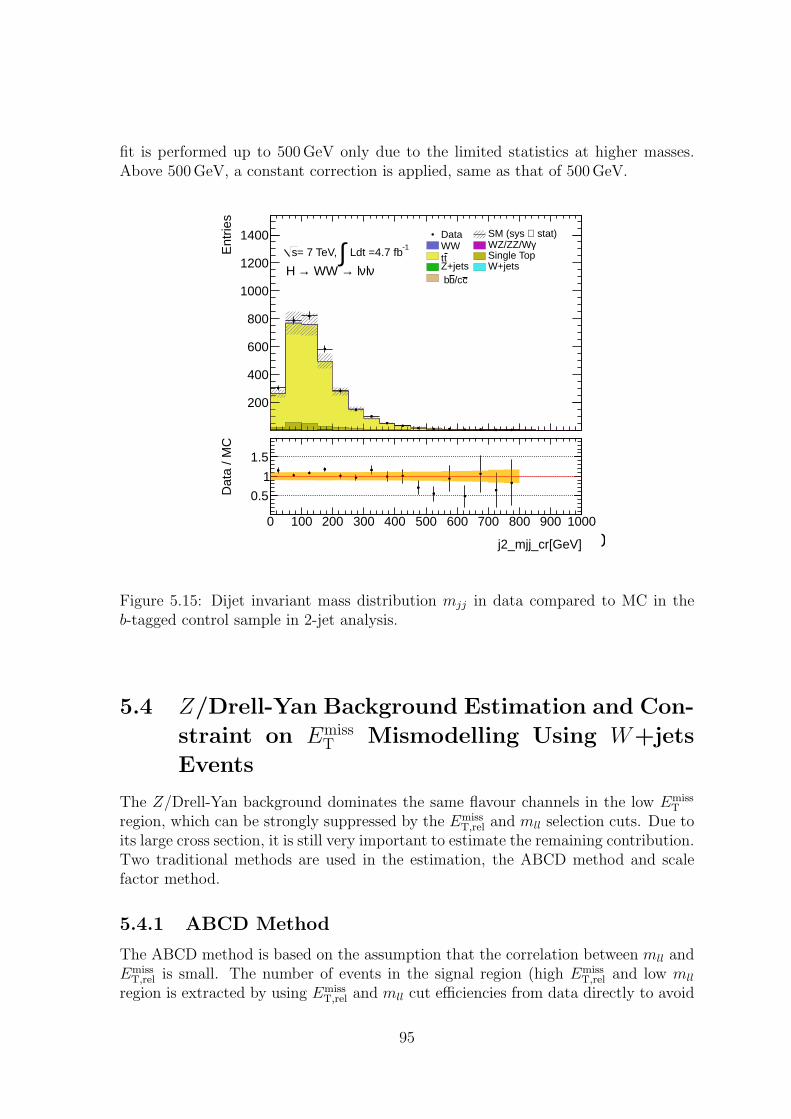
fit is performed up to 500 GeV only due to the limited statistics at higher masses.Above 500 GeV, a constant correction is applied, same as that of 500 GeV.
0 1002003004005006007008009001000
Ent
ries
200
400
600
800
1000
1200
1400-1
Ldt =4.7 fb∫= 7 TeV, s
νlν l→ WW →H
Data stat)⊕SM (sys WW γWZ/ZZ/Wtt Single TopZ+jets W+jets
c/cb b
0 100 200 300 400 500 600 700 800 900 1000
Ent
ries
200
400
600
800
1000
1200
1400-1 Ldt =4.7 fb∫= 7 TeV, s
νlν l→ WW →H
Data stat)⊕SM (sys WW γWZ/ZZ/Wtt Single Top
Z+jets W+jetsc/cb b
j2_mjj_cr[GeV]
0 100 200 300 400 500 600 700 800 900 1000
Dat
a / M
C
0.5
1
1.5
Figure 5.15: Dijet invariant mass distribution mjj in data compared to MC in theb-tagged control sample in 2-jet analysis.
5.4 Z/Drell-Yan Background Estimation and Con-
straint on EmissT Mismodelling Using W+jets
Events
The Z/Drell-Yan background dominates the same flavour channels in the low EmissT
region, which can be strongly suppressed by the EmissT,rel and mll selection cuts. Due to
its large cross section, it is still very important to estimate the remaining contribution.Two traditional methods are used in the estimation, the ABCD method and scalefactor method.
5.4.1 ABCD Method
The ABCD method is based on the assumption that the correlation between mll andEmiss
T,rel is small. The number of events in the signal region (high EmissT,rel and low mll
region is extracted by using EmissT,rel and mll cut efficiencies from data directly to avoid
95
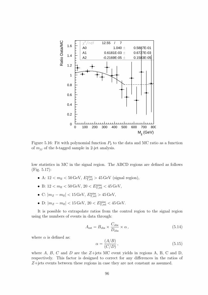
0
0.2
0.4
0.6
0.8
1
1.2
1.4
1.6
0 100 200 300 400 500 600 700 800
12.55 / 7
A0 1.040 0.5887E-01
A1 0.6181E-03 0.6727E-03
A2 -0.2169E-05 0.1583E-05
Mjj (GeV)
Rat
io D
ata/
MC
Figure 5.16: Fit with polynomial function P2 to the data and MC ratio as a functionof mjj of the b-tagged sample in 2-jet analysis.
low statistics in MC in the signal region. The ABCD regions are defined as follows(Fig. 5.17):
• A: 12 < mll < 50GeV, EmissT,rel > 45GeV (signal region),
• B: 12 < mll < 50GeV, 20 < EmissT,rel < 45GeV,
• C: |mZ −mll| < 15GeV, EmissT,rel > 45GeV,
• D: |mZ −mll| < 15GeV, 20 < EmissT,rel < 45GeV.
It is possible to extrapolate ratios from the control region to the signal regionusing the numbers of events in data through:
Aest = Bobs ×Cobs
Dobs
× α , (5.14)
where α is defined as:
α =(A/B)
(C/D), (5.15)
where A, B, C and D are the Z+jets MC event yields in regions A, B, C and D,respectively. This factor is designed to correct for any differences in the ratios ofZ+jets events between these regions in case they are not constant as assumed.
96
Dat
a E
vent
s
0
200
400
600
800
1000
1200
1400
1600
[GeV]eem0 20 40 60 80 100 120 140 160 180 200
[GeV
]m
iss
T,R
elE
0
10
20
30
40
50
60
70
80ee 1 Jet
C
D
A
B
ATLAS Preliminary
= 7 TeVs-1 Ldt = 4.71 fb∫
Figure 5.17: Regions of A, B, C and D in mll − EmissT,rel plane used for the ABCD
method and shown with data events in the ee 1-jet channel after the jet multiplicitycut.
The expected contamination from backgrounds such as diboson or top events issubtracted from the number of observed events in regions B, C and D using MCprediction of these backgrounds. The contamination is genrally small compared tothe number of Z/DY events. The number of events estimated using the ABCDmethod is thus independent of the Z/DY MC.
The ABCD estimate can be calculated after each cut in the cutflow, but topologicalcuts with a dependence on either mll or Emiss
T will have different efficiencies in theB/C/D regions and skew the resulting estimate. The systematic of this method variesfrom 15% to 34%, in different jet bins and lepton flavor combination.
5.4.2 Scale Factor Method
The scale factor method is another approach to estimate the Z/DY background insignal region A:
Aest =Cdata
Cdata +Ddata
CMC +DMC
CMC
. (5.16)
in which the region D is slightly different from ABCD method, which includes all lowEmiss
T area in Z mass window.The result is shown in Tabs. 5.10 and 5.11 for the ee and µµ channels, respectively,
in comparison with the MC prediction and the estimation using the ABCD method.This method also assumes that there is no dependence on Emiss
T for Z/DY eventsinside and outside of the Z mass window. Therefore it has the similar problem asthe ABCD method in that the normalisation factor (i.e. the ratio of the data-drivenestimate over the MC prediction) may have a strong dependence in the cutflow. Forthis reason, an alternative method is studied and described in the next section.
97
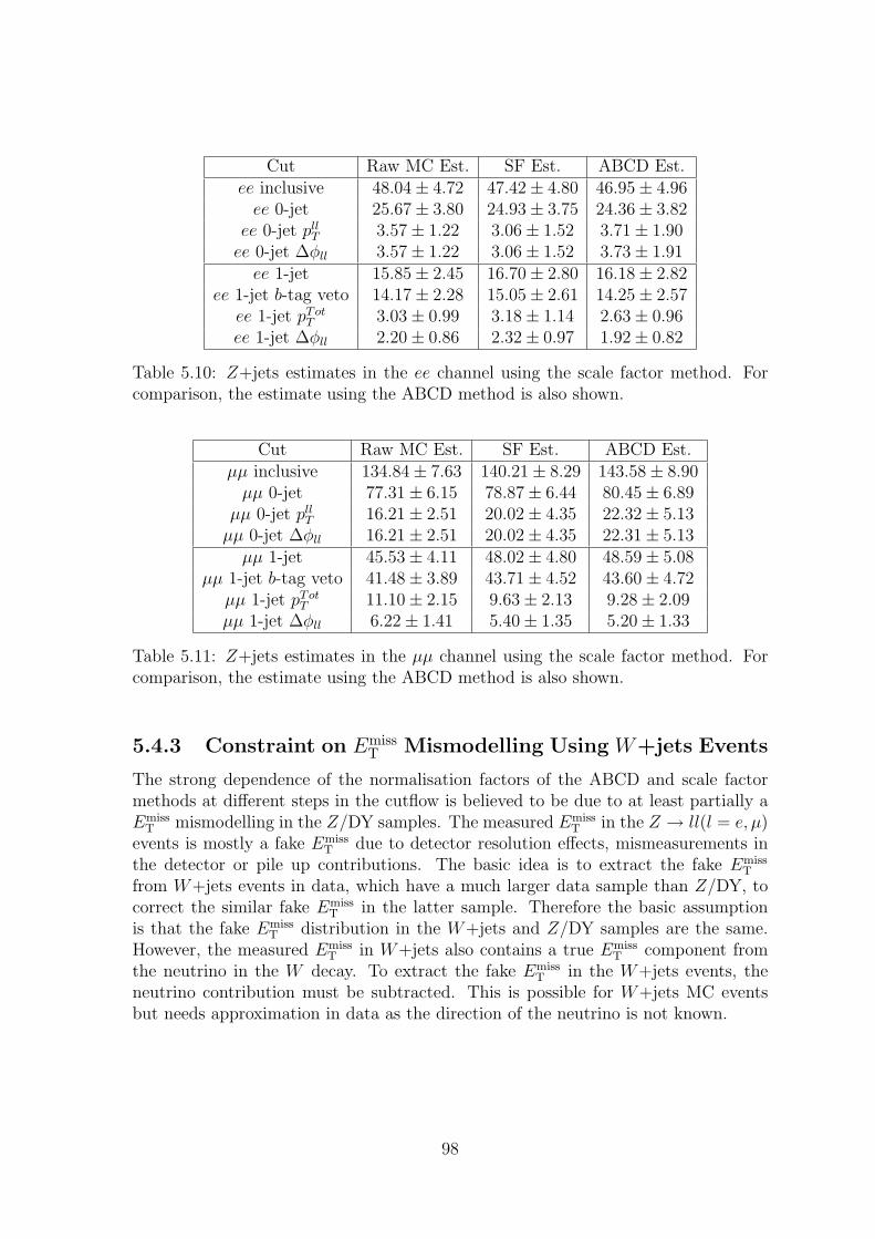
Cut Raw MC Est. SF Est. ABCD Est.ee inclusive 48.04 ± 4.72 47.42 ± 4.80 46.95 ± 4.96ee 0-jet 25.67 ± 3.80 24.93 ± 3.75 24.36 ± 3.82
ee 0-jet pllT 3.57 ± 1.22 3.06 ± 1.52 3.71 ± 1.90
ee 0-jet ∆φll 3.57 ± 1.22 3.06 ± 1.52 3.73 ± 1.91ee 1-jet 15.85 ± 2.45 16.70 ± 2.80 16.18 ± 2.82
ee 1-jet b-tag veto 14.17 ± 2.28 15.05 ± 2.61 14.25 ± 2.57ee 1-jet pTot
T 3.03 ± 0.99 3.18 ± 1.14 2.63 ± 0.96ee 1-jet ∆φll 2.20 ± 0.86 2.32 ± 0.97 1.92 ± 0.82
Table 5.10: Z+jets estimates in the ee channel using the scale factor method. Forcomparison, the estimate using the ABCD method is also shown.
Cut Raw MC Est. SF Est. ABCD Est.µµ inclusive 134.84 ± 7.63 140.21 ± 8.29 143.58 ± 8.90µµ 0-jet 77.31 ± 6.15 78.87 ± 6.44 80.45 ± 6.89
µµ 0-jet pllT 16.21 ± 2.51 20.02 ± 4.35 22.32 ± 5.13
µµ 0-jet ∆φll 16.21 ± 2.51 20.02 ± 4.35 22.31 ± 5.13µµ 1-jet 45.53 ± 4.11 48.02 ± 4.80 48.59 ± 5.08
µµ 1-jet b-tag veto 41.48 ± 3.89 43.71 ± 4.52 43.60 ± 4.72µµ 1-jet pTot
T 11.10 ± 2.15 9.63 ± 2.13 9.28 ± 2.09µµ 1-jet ∆φll 6.22 ± 1.41 5.40 ± 1.35 5.20 ± 1.33
Table 5.11: Z+jets estimates in the µµ channel using the scale factor method. Forcomparison, the estimate using the ABCD method is also shown.
5.4.3 Constraint on EmissT Mismodelling Using W+jets Events
The strong dependence of the normalisation factors of the ABCD and scale factormethods at different steps in the cutflow is believed to be due to at least partially aEmiss
T mismodelling in the Z/DY samples. The measured EmissT in the Z → ll(l = e, µ)
events is mostly a fake EmissT due to detector resolution effects, mismeasurements in
the detector or pile up contributions. The basic idea is to extract the fake EmissT
from W+jets events in data, which have a much larger data sample than Z/DY, tocorrect the similar fake Emiss
T in the latter sample. Therefore the basic assumptionis that the fake Emiss
T distribution in the W+jets and Z/DY samples are the same.However, the measured Emiss
T in W+jets also contains a true EmissT component from
the neutrino in the W decay. To extract the fake EmissT in the W+jets events, the
neutrino contribution must be subtracted. This is possible for W+jets MC eventsbut needs approximation in data as the direction of the neutrino is not known.
98
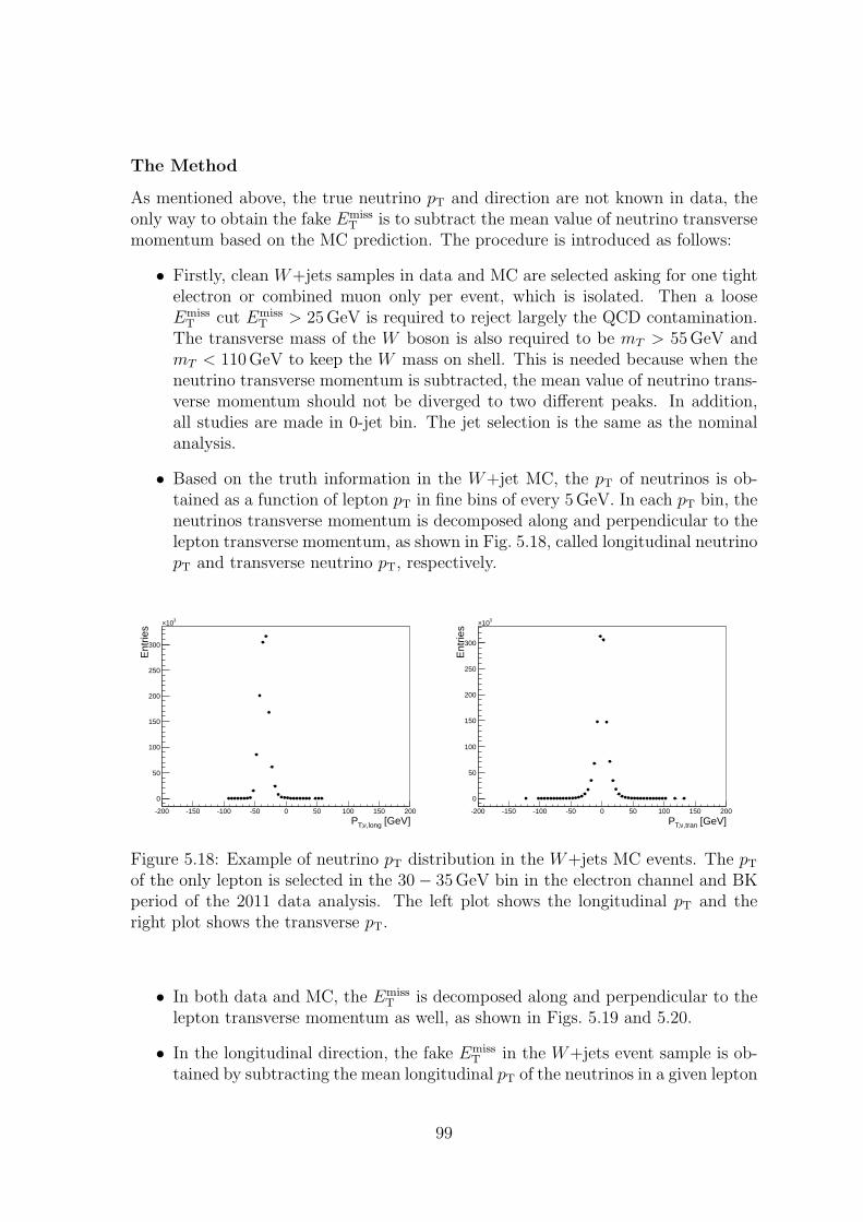
The Method
As mentioned above, the true neutrino pT and direction are not known in data, theonly way to obtain the fake Emiss
T is to subtract the mean value of neutrino transversemomentum based on the MC prediction. The procedure is introduced as follows:
• Firstly, clean W+jets samples in data and MC are selected asking for one tightelectron or combined muon only per event, which is isolated. Then a looseEmiss
T cut EmissT > 25GeV is required to reject largely the QCD contamination.
The transverse mass of the W boson is also required to be mT > 55GeV andmT < 110 GeV to keep the W mass on shell. This is needed because when theneutrino transverse momentum is subtracted, the mean value of neutrino trans-verse momentum should not be diverged to two different peaks. In addition,all studies are made in 0-jet bin. The jet selection is the same as the nominalanalysis.
• Based on the truth information in the W+jet MC, the pT of neutrinos is ob-tained as a function of lepton pT in fine bins of every 5 GeV. In each pT bin, theneutrinos transverse momentum is decomposed along and perpendicular to thelepton transverse momentum, as shown in Fig. 5.18, called longitudinal neutrinopT and transverse neutrino pT, respectively.
[GeV],longνT,P-200 -150 -100 -50 0 50 100 150 200
Ent
ries
0
50
100
150
200
250
300
310×
[GeV],tranνT,P-200 -150 -100 -50 0 50 100 150 200
Ent
ries
0
50
100
150
200
250
300
310×
Figure 5.18: Example of neutrino pT distribution in the W+jets MC events. The pT
of the only lepton is selected in the 30 − 35GeV bin in the electron channel and BKperiod of the 2011 data analysis. The left plot shows the longitudinal pT and theright plot shows the transverse pT.
• In both data and MC, the EmissT is decomposed along and perpendicular to the
lepton transverse momentum as well, as shown in Figs. 5.19 and 5.20.
• In the longitudinal direction, the fake EmissT in the W+jets event sample is ob-
tained by subtracting the mean longitudinal pT of the neutrinos in a given lepton
99
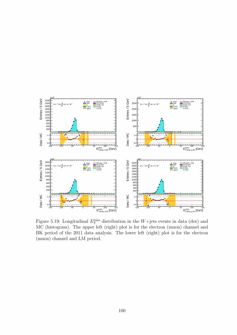
Ent
ries
/ 5 G
eV
200400600800
1000120014001600180020002200
310×
-1 Ldt =4.7 fb∫= 7 TeV, s
Data stat)⊕SM (sys WW γWZ/ZZ/Wtt Single Top
Z+jets W+jetsc/cb b H [125]
[GeV]missT,long, e,bkE
-150 -100 -50 0 50 100 150Dat
a / M
C
0.8
1
1.2
Ent
ries
/ 5 G
eV500
1000
1500
2000
2500
310×
-1 Ldt =4.7 fb∫= 7 TeV, s
Data stat)⊕SM (sys WW γWZ/ZZ/Wtt Single Top
Z+jets W+jetsc/cb b H [125]
[GeV]miss,bkµT,long, E
-150 -100 -50 0 50 100 150Dat
a / M
C
0.8
1
1.2
Ent
ries
/ 5 G
eV
200
400
600
800
1000
1200
1400
1600
1800
310×
-1 Ldt =4.7 fb∫= 7 TeV, s
Data stat)⊕SM (sys WW γWZ/ZZ/Wtt Single Top
Z+jets W+jetsc/cb b H [125]
[GeV]missT,long, e,lmE
-150 -100 -50 0 50 100 150Dat
a / M
C
0.8
1
1.2
Ent
ries
/ 5 G
eV
200400600800
1000120014001600180020002200
310×
-1 Ldt =4.7 fb∫= 7 TeV, s
Data stat)⊕SM (sys WW γWZ/ZZ/Wtt Single Top
Z+jets W+jetsc/cb b H [125]
[GeV]miss,lmµT,long, E
-150 -100 -50 0 50 100 150Dat
a / M
C
0.8
1
1.2
Figure 5.19: Longitudinal EmissT distribution in the W+jets events in data (dot) and
MC (histogram). The upper left (right) plot is for the electron (muon) channel andBK period of the 2011 data analysis. The lower left (right) plot is for the electron(muon) channel and LM period.
100
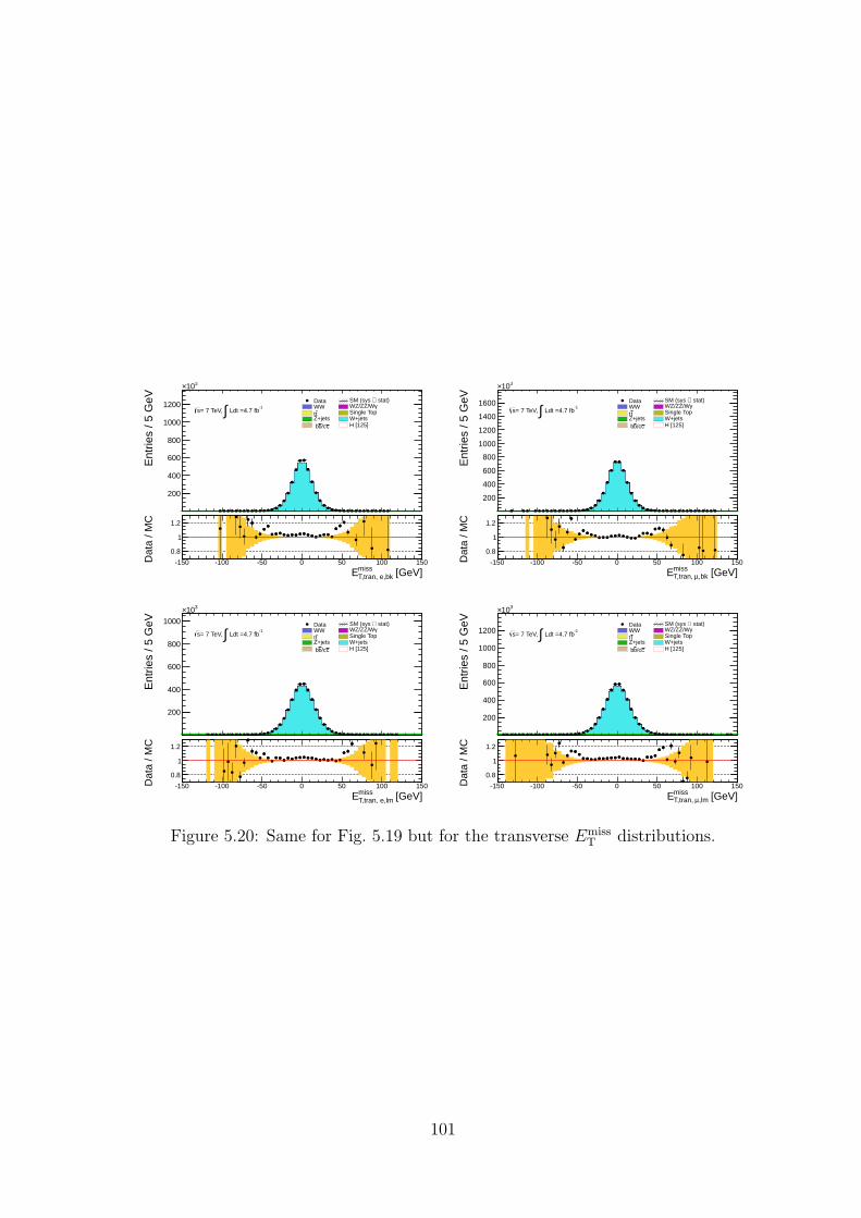
Ent
ries
/ 5 G
eV
200
400
600
800
1000
1200
310×
-1 Ldt =4.7 fb∫= 7 TeV, s
Data stat)⊕SM (sys WW γWZ/ZZ/Wtt Single Top
Z+jets W+jetsc/cb b H [125]
[GeV]missT,tran, e,bkE
-150 -100 -50 0 50 100 150Dat
a / M
C
0.8
1
1.2
Ent
ries
/ 5 G
eV
200
400
600
800
1000
1200
1400
1600
310×
-1 Ldt =4.7 fb∫= 7 TeV, s
Data stat)⊕SM (sys WW γWZ/ZZ/Wtt Single Top
Z+jets W+jetsc/cb b H [125]
[GeV]miss,bkµT,tran, E
-150 -100 -50 0 50 100 150Dat
a / M
C
0.8
1
1.2
Ent
ries
/ 5 G
eV
200
400
600
800
1000
310×
-1 Ldt =4.7 fb∫= 7 TeV, s
Data stat)⊕SM (sys WW γWZ/ZZ/Wtt Single Top
Z+jets W+jetsc/cb b H [125]
[GeV]missT,tran, e,lmE
-150 -100 -50 0 50 100 150Dat
a / M
C
0.8
1
1.2
Ent
ries
/ 5 G
eV
200
400
600
800
1000
1200
310×
-1 Ldt =4.7 fb∫= 7 TeV, s
Data stat)⊕SM (sys WW γWZ/ZZ/Wtt Single Top
Z+jets W+jetsc/cb b H [125]
[GeV]miss,lmµT,tran, E
-150 -100 -50 0 50 100 150Dat
a / M
C
0.8
1
1.2
Figure 5.20: Same for Fig. 5.19 but for the transverse EmissT distributions.
101
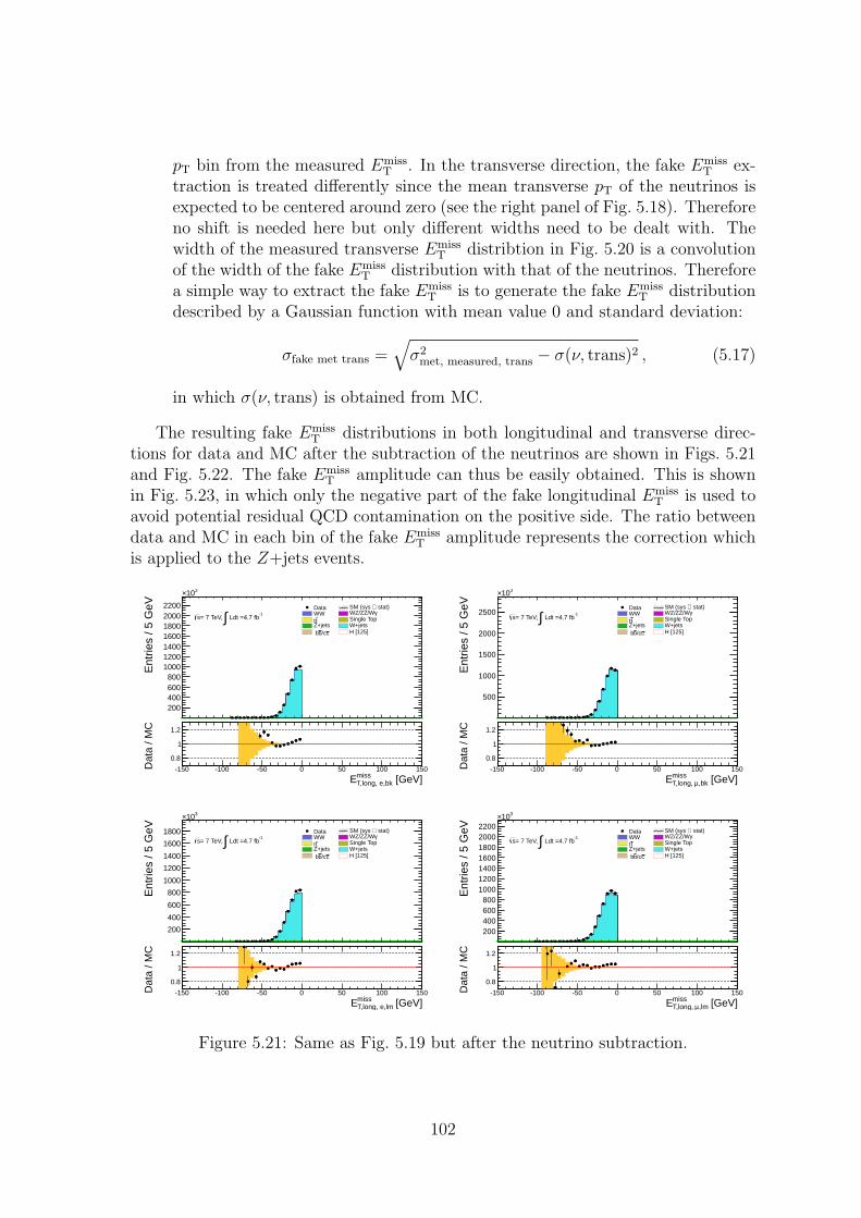
pT bin from the measured EmissT . In the transverse direction, the fake Emiss
T ex-traction is treated differently since the mean transverse pT of the neutrinos isexpected to be centered around zero (see the right panel of Fig. 5.18). Thereforeno shift is needed here but only different widths need to be dealt with. Thewidth of the measured transverse Emiss
T distribtion in Fig. 5.20 is a convolutionof the width of the fake Emiss
T distribution with that of the neutrinos. Thereforea simple way to extract the fake Emiss
T is to generate the fake EmissT distribution
described by a Gaussian function with mean value 0 and standard deviation:
σfake met trans =√
σ2met, measured, trans − σ(ν, trans)2 , (5.17)
in which σ(ν, trans) is obtained from MC.
The resulting fake EmissT distributions in both longitudinal and transverse direc-
tions for data and MC after the subtraction of the neutrinos are shown in Figs. 5.21and Fig. 5.22. The fake Emiss
T amplitude can thus be easily obtained. This is shownin Fig. 5.23, in which only the negative part of the fake longitudinal Emiss
T is used toavoid potential residual QCD contamination on the positive side. The ratio betweendata and MC in each bin of the fake Emiss
T amplitude represents the correction whichis applied to the Z+jets events.
Ent
ries
/ 5 G
eV
200400600800
1000120014001600180020002200
310×
-1 Ldt =4.7 fb∫= 7 TeV, s
Data stat)⊕SM (sys WW γWZ/ZZ/Wtt Single Top
Z+jets W+jetsc/cb b H [125]
[GeV]missT,long, e,bkE
-150 -100 -50 0 50 100 150Dat
a / M
C
0.8
1
1.2
Ent
ries
/ 5 G
eV
500
1000
1500
2000
2500
310×
-1 Ldt =4.7 fb∫= 7 TeV, s
Data stat)⊕SM (sys WW γWZ/ZZ/Wtt Single Top
Z+jets W+jetsc/cb b H [125]
[GeV]miss,bkµT,long, E
-150 -100 -50 0 50 100 150Dat
a / M
C
0.8
1
1.2
Ent
ries
/ 5 G
eV
200
400
600
800
1000
1200
1400
1600
1800
310×
-1 Ldt =4.7 fb∫= 7 TeV, s
Data stat)⊕SM (sys WW γWZ/ZZ/Wtt Single Top
Z+jets W+jetsc/cb b H [125]
[GeV]missT,long, e,lmE
-150 -100 -50 0 50 100 150Dat
a / M
C
0.8
1
1.2
Ent
ries
/ 5 G
eV
200400600800
1000120014001600180020002200
310×
-1 Ldt =4.7 fb∫= 7 TeV, s
Data stat)⊕SM (sys WW γWZ/ZZ/Wtt Single Top
Z+jets W+jetsc/cb b H [125]
[GeV]miss,lmµT,long, E
-150 -100 -50 0 50 100 150Dat
a / M
C
0.8
1
1.2
Figure 5.21: Same as Fig. 5.19 but after the neutrino subtraction.
102
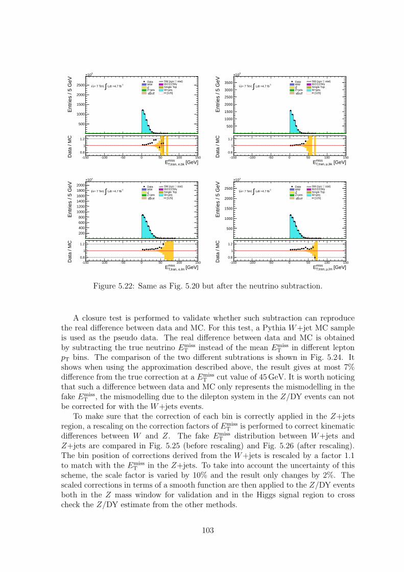
Ent
ries
/ 5 G
eV
500
1000
1500
2000
2500
310×
-1 Ldt =4.7 fb∫= 7 TeV, s
Data stat)⊕SM (sys WW γWZ/ZZ/Wtt Single Top
Z+jets W+jetsc/cb b H [125]
[GeV]missT,tran, e,bkE
-150 -100 -50 0 50 100 150Dat
a / M
C
0.8
1
1.2
Ent
ries
/ 5 G
eV
500
1000
1500
2000
2500
3000
3500
310×
-1 Ldt =4.7 fb∫= 7 TeV, s
Data stat)⊕SM (sys WW γWZ/ZZ/Wtt Single Top
Z+jets W+jetsc/cb b H [125]
[GeV]miss,bkµT,tran, E
-150 -100 -50 0 50 100 150Dat
a / M
C
0.8
1
1.2
Ent
ries
/ 5 G
eV
200
400
600
800
1000
1200
1400
1600
1800
2000
310×
-1 Ldt =4.7 fb∫= 7 TeV, s
Data stat)⊕SM (sys WW γWZ/ZZ/Wtt Single Top
Z+jets W+jetsc/cb b H [125]
[GeV]missT,tran, e,lmE
-150 -100 -50 0 50 100 150Dat
a / M
C
0.8
1
1.2
Ent
ries
/ 5 G
eV
500
1000
1500
2000
2500
310×
-1 Ldt =4.7 fb∫= 7 TeV, s
Data stat)⊕SM (sys WW γWZ/ZZ/Wtt Single Top
Z+jets W+jetsc/cb b H [125]
[GeV]miss,lmµT,tran, E
-150 -100 -50 0 50 100 150Dat
a / M
C
0.8
1
1.2
Figure 5.22: Same as Fig. 5.20 but after the neutrino subtraction.
A closure test is performed to validate whether such subtraction can reproducethe real difference between data and MC. For this test, a Pythia W+jet MC sampleis used as the pseudo data. The real difference between data and MC is obtainedby subtracting the true neutrino Emiss
T instead of the mean EmissT in different lepton
pT bins. The comparison of the two different subtrations is shown in Fig. 5.24. Itshows when using the approximation described above, the result gives at most 7%difference from the true correction at a Emiss
T cut value of 45 GeV. It is worth noticingthat such a difference between data and MC only represents the mismodelling in thefake Emiss
T , the mismodelling due to the dilepton system in the Z/DY events can notbe corrected for with the W+jets events.
To make sure that the correction of each bin is correctly applied in the Z+jetsregion, a rescaling on the correction factors of Emiss
T is performed to correct kinematicdifferences between W and Z. The fake Emiss
T distribution between W+jets andZ+jets are compared in Fig. 5.25 (before rescaling) and Fig. 5.26 (after rescaling).The bin position of corrections derived from the W+jets is rescaled by a factor 1.1to match with the Emiss
T in the Z+jets. To take into account the uncertainty of thisscheme, the scale factor is varied by 10% and the result only changes by 2%. Thescaled corrections in terms of a smooth function are then applied to the Z/DY eventsboth in the Z mass window for validation and in the Higgs signal region to crosscheck the Z/DY estimate from the other methods.
103
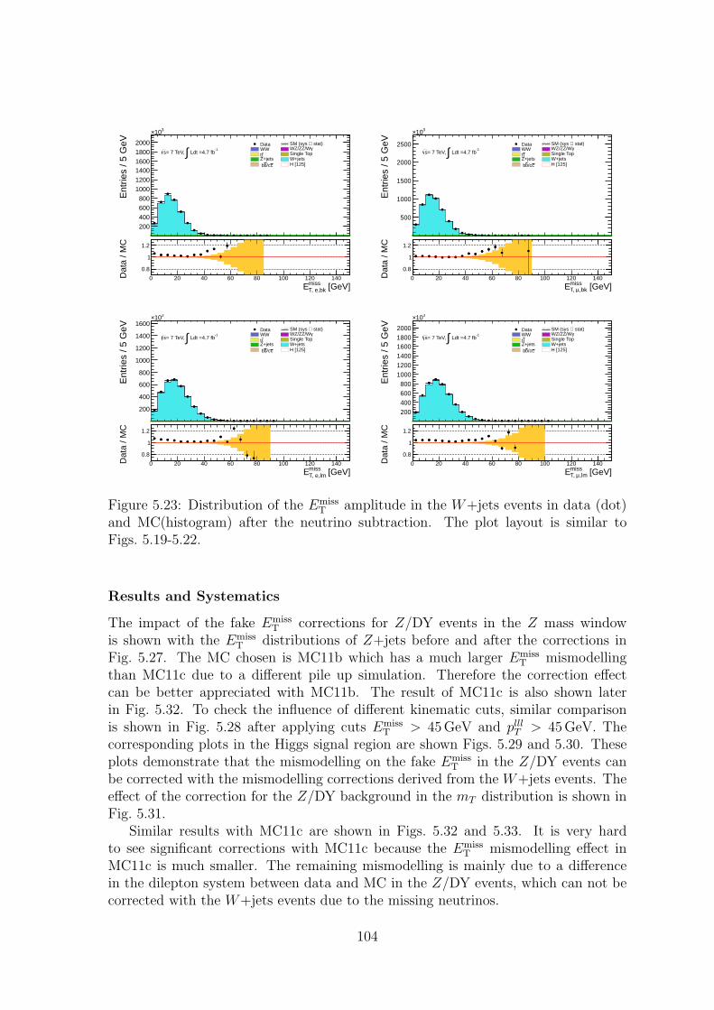
Ent
ries
/ 5 G
eV
200
400
600
800
1000
1200
14001600
1800
2000
310×
-1 Ldt =4.7 fb∫= 7 TeV, s
Data stat)⊕SM (sys WW γWZ/ZZ/Wtt Single Top
Z+jets W+jetsc/cb b H [125]
[GeV]missT, e,bkE
0 20 40 60 80 100 120 140Dat
a / M
C
0.8
1
1.2
Ent
ries
/ 5 G
eV
500
1000
1500
2000
2500
310×
-1 Ldt =4.7 fb∫= 7 TeV, s
Data stat)⊕SM (sys WW γWZ/ZZ/Wtt Single Top
Z+jets W+jetsc/cb b H [125]
[GeV]miss,bkµT, E
0 20 40 60 80 100 120 140Dat
a / M
C
0.8
1
1.2
Ent
ries
/ 5 G
eV
200
400
600
800
1000
1200
1400
1600
310×
-1 Ldt =4.7 fb∫= 7 TeV, s
Data stat)⊕SM (sys WW γWZ/ZZ/Wtt Single Top
Z+jets W+jetsc/cb b H [125]
[GeV]missT, e,lmE
0 20 40 60 80 100 120 140Dat
a / M
C
0.8
1
1.2
Ent
ries
/ 5 G
eV
200
400
600
800
1000
1200
1400
16001800
2000
310×
-1 Ldt =4.7 fb∫= 7 TeV, s
Data stat)⊕SM (sys WW γWZ/ZZ/Wtt Single Top
Z+jets W+jetsc/cb b H [125]
[GeV]miss,lmµT, E
0 20 40 60 80 100 120 140Dat
a / M
C
0.8
1
1.2
Figure 5.23: Distribution of the EmissT amplitude in the W+jets events in data (dot)
and MC(histogram) after the neutrino subtraction. The plot layout is similar toFigs. 5.19-5.22.
Results and Systematics
The impact of the fake EmissT corrections for Z/DY events in the Z mass window
is shown with the EmissT distributions of Z+jets before and after the corrections in
Fig. 5.27. The MC chosen is MC11b which has a much larger EmissT mismodelling
than MC11c due to a different pile up simulation. Therefore the correction effectcan be better appreciated with MC11b. The result of MC11c is also shown laterin Fig. 5.32. To check the influence of different kinematic cuts, similar comparisonis shown in Fig. 5.28 after applying cuts Emiss
T > 45GeV and plllT > 45GeV. The
corresponding plots in the Higgs signal region are shown Figs. 5.29 and 5.30. Theseplots demonstrate that the mismodelling on the fake Emiss
T in the Z/DY events canbe corrected with the mismodelling corrections derived from the W+jets events. Theeffect of the correction for the Z/DY background in the mT distribution is shown inFig. 5.31.
Similar results with MC11c are shown in Figs. 5.32 and 5.33. It is very hardto see significant corrections with MC11c because the Emiss
T mismodelling effect inMC11c is much smaller. The remaining mismodelling is mainly due to a differencein the dilepton system between data and MC in the Z/DY events, which can not becorrected with the W+jets events due to the missing neutrinos.
104
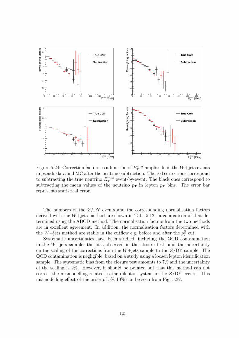
[GeV]missTE
0 20 40 60 80 100 120 140
Rew
eigh
ting
fact
ors
0
0.2
0.4
0.6
0.8
1
1.2
True Corr
Subtraction
[GeV]missTE
0 20 40 60 80 100 120 140
Rew
eigh
ting
fact
ors
0
0.2
0.4
0.6
0.8
1
1.2
1.4
True Corr
Subtraction
[GeV]missTE
0 20 40 60 80 100 120 140
Rew
eigh
ting
fact
ors
0
0.5
1
1.5
2
True Corr
Subtraction
[GeV]missTE
0 20 40 60 80 100 120 140
Rew
eigh
ting
fact
ors
0
0.2
0.4
0.6
0.8
1 True Corr
Subtraction
Figure 5.24: Correction factors as a function of EmissT amplitude in the W+jets events
in pseudo data and MC after the neutrino subtraction. The red corrections correspondto subtracting the true neutrino Emiss
T event-by-event. The black ones correspond tosubtracting the mean values of the neutrino pT in lepton pT bins. The error barrepresents statistical error.
The numbers of the Z/DY events and the corresponding normalisation factorsderived with the W+jets method are shown in Tab. 5.12, in comparison of that de-termined using the ABCD method. The normalisation factors from the two methodsare in excellent agreement. In addition, the normalisation factors determined withthe W+jets method are stable in the cutflow e.g. before and after the pll
T cut.Systematic uncertainties have been studied, including the QCD contamination
in the W+jets sample, the bias observed in the closure test, and the uncertaintyon the scaling of the corrections from the W+jets sample to the Z/DY sample. TheQCD contamination is negligible, based on a study using a loosen lepton identificationsample. The systematic bias from the closure test amounts to 7% and the uncertaintyof the scaling is 2%. However, it should be pointed out that this method can notcorrect the mismodelling related to the dilepton system in the Z/DY events. Thismismodelling effect of the order of 5%-10% can be seen from Fig. 5.32.
105
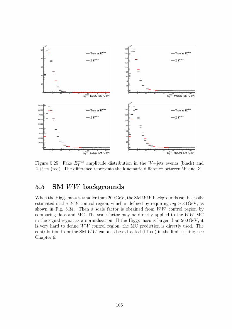
_ELEC_BK [GeV] missTE
0 20 40 60 80 100 120 1400
20
40
60
80
100
310×
missTTrue W E
missTZ E
_MUON_BK [GeV] missTE
0 20 40 60 80 100 120 140
0
20
40
60
80
100
120
140
160
180
310×
missTTrue W E
missTZ E
_ELEC_LM [GeV] missTE
0 20 40 60 80 100 120 140
0
10000
20000
30000
40000
50000
60000
70000
80000
90000
missTTrue W E
missTZ E
_MUON_LM [GeV] missTE
0 20 40 60 80 100 120 140
0
20
40
60
80
100
120
140
310×
missTTrue W E
missTZ E
Figure 5.25: Fake EmissT amplitude distribution in the W+jets events (black) and
Z+jets (red). The difference represents the kinematic difference between W and Z.
5.5 SM WW backgrounds
When the Higgs mass is smaller than 200 GeV, the SMWW backgrounds can be easilyestimated in the WW control region, which is defined by requiring mll > 80GeV, asshown in Fig. 5.34. Then a scale factor is obtained from WW control region bycomparing data and MC. The scale factor may be directly applied to the WW MCin the signal region as a normalization. If the Higgs mass is larger than 200 GeV, itis very hard to define WW control region, the MC prediction is directly used. Thecontribution from the SM WW can also be extracted (fitted) in the limit setting, seeChapter 6.
106
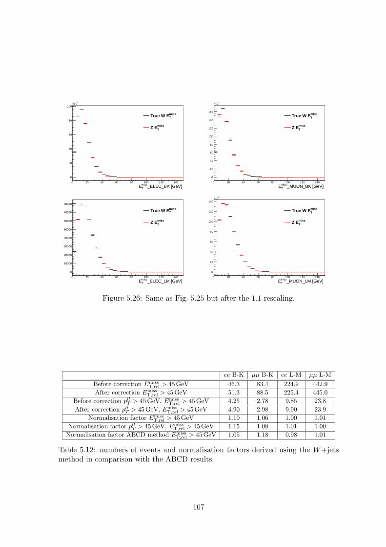
_ELEC_BK [GeV] missTE
0 20 40 60 80 100 120 140
0
20
40
60
80
100
310×
missTTrue W E
missTZ E
_MUON_BK [GeV] missTE
0 20 40 60 80 100 120 140
0
20
40
60
80
100
120
140
160
310×
missTTrue W E
missTZ E
_ELEC_LM [GeV] missTE
0 20 40 60 80 100 120 140
0
10000
20000
30000
40000
50000
60000
70000
80000
missTTrue W E
missTZ E
_MUON_LM [GeV] missTE
0 20 40 60 80 100 120 140
0
20
40
60
80
100
120
140
310×
missTTrue W E
missTZ E
Figure 5.26: Same as Fig. 5.25 but after the 1.1 rescaling.
ee B-K µµ B-K ee L-M µµ L-M
Before correction EmissT,rel > 45 GeV 46.3 83.4 224.9 442.9
After correction EmissT,rel > 45 GeV 51.3 88.5 225.4 445.0
Before correction pllT > 45 GeV, Emiss
T,rel > 45 GeV 4.25 2.78 9.85 23.8
After correction pllT > 45 GeV, Emiss
T,rel > 45 GeV 4.90 2.98 9.90 23.9
Normalisation factor EmissT,rel > 45 GeV 1.10 1.06 1.00 1.01
Normalisation factor pllT > 45 GeV, Emiss
T,rel > 45 GeV 1.15 1.08 1.01 1.00
Normalisation factor ABCD method EmissT,rel > 45 GeV 1.05 1.18 0.98 1.01
Table 5.12: numbers of events and normalisation factors derived using the W+jetsmethod in comparison with the ABCD results.
107
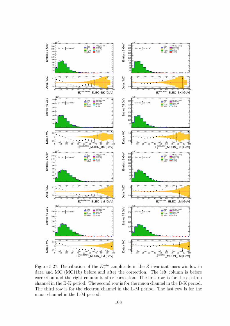
Ent
ries
/ 5 G
eV
20
406080
100120140
160180200220
310×
-1 Ldt =4.7 fb∫= 7 TeV, s
Data stat)⊕SM (sys WW γWZ/ZZ/Wtt Single Top
Z+jets W+jetsc/cb b H [125]
_ELEC_BK [GeV]miss beforeTE
0 10 20 30 40 50 60 70 80 90 100Dat
a / M
C
0.8
1
1.2
Ent
ries
/ 5 G
eV
20406080
100120140160180200220
310×
-1 Ldt =4.7 fb∫= 7 TeV, s
Data stat)⊕SM (sys WW γWZ/ZZ/Wtt Single Top
Z+jets W+jetsc/cb b H [125]
_ELEC_BK [GeV]miss afterTE
0 10 20 30 40 50 60 70 80 90 100Dat
a / M
C
0.8
1
1.2
Ent
ries
/ 5 G
eV
50
100
150
200
250
300
350
310×
-1 Ldt =4.7 fb∫= 7 TeV, s
Data stat)⊕SM (sys WW γWZ/ZZ/Wtt Single Top
Z+jets W+jetsc/cb b H [125]
_MUON_BK [GeV]miss beforeTE
0 10 20 30 40 50 60 70 80 90 100Dat
a / M
C
0.8
1
1.2
Ent
ries
/ 5 G
eV50
100
150
200
250
300
350
310×
-1 Ldt =4.7 fb∫= 7 TeV, s
Data stat)⊕SM (sys WW γWZ/ZZ/Wtt Single Top
Z+jets W+jetsc/cb b H [125]
_MUON_BK [GeV]miss afterTE
0 10 20 30 40 50 60 70 80 90 100Dat
a / M
C
0.8
1
1.2
Ent
ries
/ 5 G
eV
20
40
60
80
100
120
140
160
180310×
-1 Ldt =4.7 fb∫= 7 TeV, s
Data stat)⊕SM (sys WW γWZ/ZZ/Wtt Single Top
Z+jets W+jetsc/cb b H [125]
_ELEC_LM [GeV]miss beforeTE
0 10 20 30 40 50 60 70 80 90 100Dat
a / M
C
0.8
1
1.2
Ent
ries
/ 5 G
eV
20
40
60
80
100
120
140
160
180
310×
-1 Ldt =4.7 fb∫= 7 TeV, s
Data stat)⊕SM (sys WW γWZ/ZZ/Wtt Single Top
Z+jets W+jetsc/cb b H [125]
_ELEC_LM [GeV]miss afterTE
0 10 20 30 40 50 60 70 80 90 100Dat
a / M
C
0.8
1
1.2
Ent
ries
/ 5 G
eV
50
100
150
200
250
310×
-1 Ldt =4.7 fb∫= 7 TeV, s
Data stat)⊕SM (sys WW γWZ/ZZ/Wtt Single Top
Z+jets W+jetsc/cb b H [125]
_MUON_LM [GeV]miss beforeTE
0 10 20 30 40 50 60 70 80 90 100Dat
a / M
C
0.8
1
1.2
Ent
ries
/ 5 G
eV
50
100
150
200
250
300310×
-1 Ldt =4.7 fb∫= 7 TeV, s
Data stat)⊕SM (sys WW γWZ/ZZ/Wtt Single Top
Z+jets W+jetsc/cb b H [125]
_MUON_LM [GeV]miss afterTE
0 10 20 30 40 50 60 70 80 90 100Dat
a / M
C
0.8
1
1.2
Figure 5.27: Distribution of the EmissT amplitude in the Z invariant mass window in
data and MC (MC11b) before and after the correction. The left column is beforecorrection and the right column is after correction. The first row is for the electronchannel in the B-K period. The second row is for the muon channel in the B-K period.The third row is for the electron channel in the L-M period. The last row is for themuon channel in the L-M period.
108
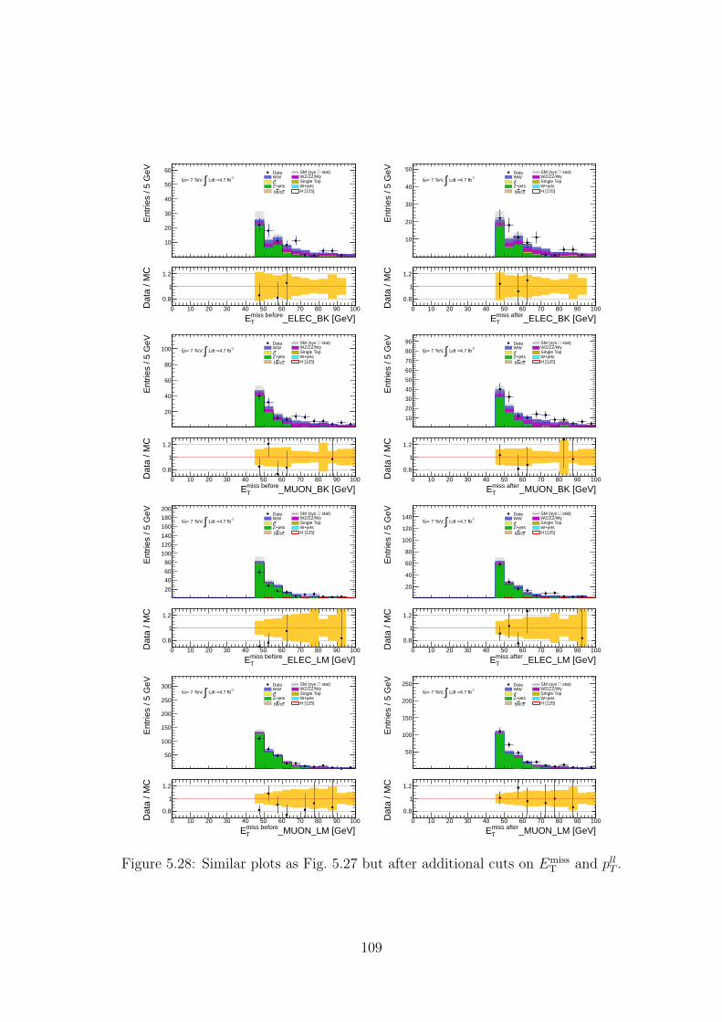
Ent
ries
/ 5 G
eV
10
20
30
40
50
60-1
Ldt =4.7 fb∫= 7 TeV, s
Data stat)⊕SM (sys WW γWZ/ZZ/Wtt Single Top
Z+jets W+jetsc/cb b H [125]
_ELEC_BK [GeV]miss beforeTE
0 10 20 30 40 50 60 70 80 90 100Dat
a / M
C
0.8
1
1.2
Ent
ries
/ 5 G
eV
10
20
30
40
50-1
Ldt =4.7 fb∫= 7 TeV, s
Data stat)⊕SM (sys WW γWZ/ZZ/Wtt Single Top
Z+jets W+jetsc/cb b H [125]
_ELEC_BK [GeV]miss afterTE
0 10 20 30 40 50 60 70 80 90 100Dat
a / M
C
0.8
1
1.2
Ent
ries
/ 5 G
eV
20
40
60
80
100 -1 Ldt =4.7 fb∫= 7 TeV, s
Data stat)⊕SM (sys WW γWZ/ZZ/Wtt Single Top
Z+jets W+jetsc/cb b H [125]
_MUON_BK [GeV]miss beforeTE
0 10 20 30 40 50 60 70 80 90 100Dat
a / M
C
0.8
1
1.2
Ent
ries
/ 5 G
eV
10
20
30
40
50
60
70
80
90-1
Ldt =4.7 fb∫= 7 TeV, s
Data stat)⊕SM (sys WW γWZ/ZZ/Wtt Single Top
Z+jets W+jetsc/cb b H [125]
_MUON_BK [GeV]miss afterTE
0 10 20 30 40 50 60 70 80 90 100Dat
a / M
C
0.8
1
1.2
Ent
ries
/ 5 G
eV
20
40
60
80
100
120
140
160
180
200
-1 Ldt =4.7 fb∫= 7 TeV, s
Data stat)⊕SM (sys WW γWZ/ZZ/Wtt Single Top
Z+jets W+jetsc/cb b H [125]
_ELEC_LM [GeV]miss beforeTE
0 10 20 30 40 50 60 70 80 90 100Dat
a / M
C
0.8
1
1.2
Ent
ries
/ 5 G
eV
20
40
60
80
100
120
140 -1 Ldt =4.7 fb∫= 7 TeV, s
Data stat)⊕SM (sys WW γWZ/ZZ/Wtt Single Top
Z+jets W+jetsc/cb b H [125]
_ELEC_LM [GeV]miss afterTE
0 10 20 30 40 50 60 70 80 90 100Dat
a / M
C
0.8
1
1.2
Ent
ries
/ 5 G
eV
50
100
150
200
250
300-1
Ldt =4.7 fb∫= 7 TeV, s
Data stat)⊕SM (sys WW γWZ/ZZ/Wtt Single Top
Z+jets W+jetsc/cb b H [125]
_MUON_LM [GeV]miss beforeTE
0 10 20 30 40 50 60 70 80 90 100Dat
a / M
C
0.8
1
1.2
Ent
ries
/ 5 G
eV
50
100
150
200
250-1
Ldt =4.7 fb∫= 7 TeV, s
Data stat)⊕SM (sys WW γWZ/ZZ/Wtt Single Top
Z+jets W+jetsc/cb b H [125]
_MUON_LM [GeV]miss afterTE
0 10 20 30 40 50 60 70 80 90 100Dat
a / M
C
0.8
1
1.2
Figure 5.28: Similar plots as Fig. 5.27 but after additional cuts on EmissT and pll
T .
109
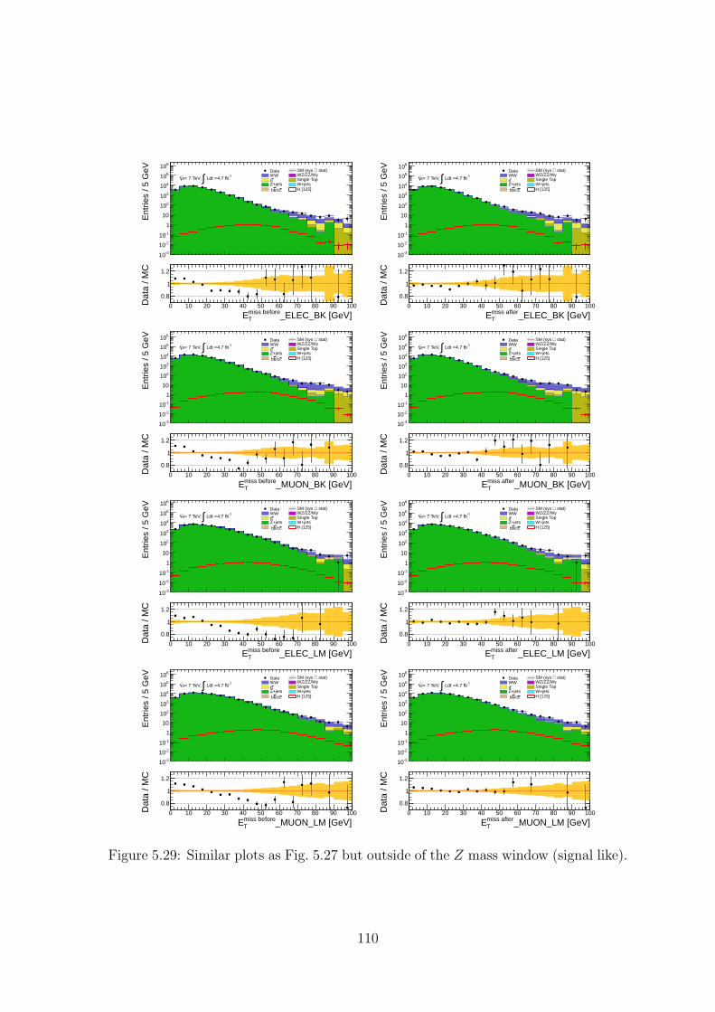
Ent
ries
/ 5 G
eV
-310
-210
-110
1
10
210
310
410
510
610
-1 Ldt =4.7 fb∫= 7 TeV, s
Data stat)⊕SM (sys WW γWZ/ZZ/Wtt Single Top
Z+jets W+jetsc/cb b H [125]
_ELEC_BK [GeV]miss beforeTE
0 10 20 30 40 50 60 70 80 90 100Dat
a / M
C
0.8
1
1.2
Ent
ries
/ 5 G
eV
-310
-210
-110
1
10
210
310
410
510
610-1
Ldt =4.7 fb∫= 7 TeV, s
Data stat)⊕SM (sys WW γWZ/ZZ/Wtt Single Top
Z+jets W+jetsc/cb b H [125]
_ELEC_BK [GeV]miss afterTE
0 10 20 30 40 50 60 70 80 90 100Dat
a / M
C
0.8
1
1.2
Ent
ries
/ 5 G
eV
-310
-210
-110
1
10
210
310
410
510
610-1
Ldt =4.7 fb∫= 7 TeV, s
Data stat)⊕SM (sys WW γWZ/ZZ/Wtt Single Top
Z+jets W+jetsc/cb b H [125]
_MUON_BK [GeV]miss beforeTE
0 10 20 30 40 50 60 70 80 90 100Dat
a / M
C
0.8
1
1.2
Ent
ries
/ 5 G
eV
-310
-210
-110
1
10
210
310
410
510
610-1
Ldt =4.7 fb∫= 7 TeV, s
Data stat)⊕SM (sys WW γWZ/ZZ/Wtt Single Top
Z+jets W+jetsc/cb b H [125]
_MUON_BK [GeV]miss afterTE
0 10 20 30 40 50 60 70 80 90 100Dat
a / M
C
0.8
1
1.2
Ent
ries
/ 5 G
eV
-310
-210
-110
1
10
210
310
410
510
610
-1 Ldt =4.7 fb∫= 7 TeV, s
Data stat)⊕SM (sys WW γWZ/ZZ/Wtt Single Top
Z+jets W+jetsc/cb b H [125]
_ELEC_LM [GeV]miss beforeTE
0 10 20 30 40 50 60 70 80 90 100Dat
a / M
C
0.8
1
1.2
Ent
ries
/ 5 G
eV
-310
-210
-110
1
10
210
310
410
510
610
-1 Ldt =4.7 fb∫= 7 TeV, s
Data stat)⊕SM (sys WW γWZ/ZZ/Wtt Single Top
Z+jets W+jetsc/cb b H [125]
_ELEC_LM [GeV]miss afterTE
0 10 20 30 40 50 60 70 80 90 100Dat
a / M
C
0.8
1
1.2
Ent
ries
/ 5 G
eV
-310
-210
-110
1
10
210
310
410
510
610-1
Ldt =4.7 fb∫= 7 TeV, s
Data stat)⊕SM (sys WW γWZ/ZZ/Wtt Single Top
Z+jets W+jetsc/cb b H [125]
_MUON_LM [GeV]miss beforeTE
0 10 20 30 40 50 60 70 80 90 100Dat
a / M
C
0.8
1
1.2
Ent
ries
/ 5 G
eV
-310
-210
-110
1
10
210
310
410
510
610-1
Ldt =4.7 fb∫= 7 TeV, s
Data stat)⊕SM (sys WW γWZ/ZZ/Wtt Single Top
Z+jets W+jetsc/cb b H [125]
_MUON_LM [GeV]miss afterTE
0 10 20 30 40 50 60 70 80 90 100Dat
a / M
C
0.8
1
1.2
Figure 5.29: Similar plots as Fig. 5.27 but outside of the Z mass window (signal like).
110
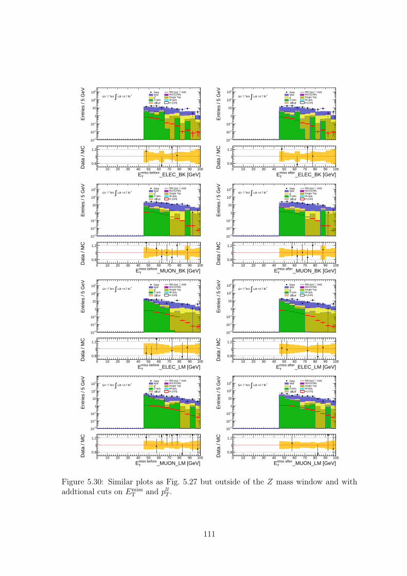
Ent
ries
/ 5 G
eV
-310
-210
-110
1
10
210
310-1
Ldt =4.7 fb∫= 7 TeV, s
Data stat)⊕SM (sys WW γWZ/ZZ/Wtt Single Top
Z+jets W+jetsc/cb b H [125]
_ELEC_BK [GeV]miss beforeTE
0 10 20 30 40 50 60 70 80 90 100Dat
a / M
C
0.8
1
1.2
Ent
ries
/ 5 G
eV
-310
-210
-110
1
10
210
310-1
Ldt =4.7 fb∫= 7 TeV, s
Data stat)⊕SM (sys WW γWZ/ZZ/Wtt Single Top
Z+jets W+jetsc/cb b H [125]
_ELEC_BK [GeV]miss afterTE
0 10 20 30 40 50 60 70 80 90 100Dat
a / M
C
0.8
1
1.2
Ent
ries
/ 5 G
eV
-310
-210
-110
1
10
210
310 -1 Ldt =4.7 fb∫= 7 TeV, s
Data stat)⊕SM (sys WW γWZ/ZZ/Wtt Single Top
Z+jets W+jetsc/cb b H [125]
_MUON_BK [GeV]miss beforeTE
0 10 20 30 40 50 60 70 80 90 100Dat
a / M
C
0.8
1
1.2
Ent
ries
/ 5 G
eV
-310
-210
-110
1
10
210
310 -1 Ldt =4.7 fb∫= 7 TeV, s
Data stat)⊕SM (sys WW γWZ/ZZ/Wtt Single Top
Z+jets W+jetsc/cb b H [125]
_MUON_BK [GeV]miss afterTE
0 10 20 30 40 50 60 70 80 90 100Dat
a / M
C
0.8
1
1.2
Ent
ries
/ 5 G
eV
-310
-210
-110
1
10
210
310 -1 Ldt =4.7 fb∫= 7 TeV, s
Data stat)⊕SM (sys WW γWZ/ZZ/Wtt Single Top
Z+jets W+jetsc/cb b H [125]
_ELEC_LM [GeV]miss beforeTE
0 10 20 30 40 50 60 70 80 90 100Dat
a / M
C
0.8
1
1.2
Ent
ries
/ 5 G
eV
-310
-210
-110
1
10
210
310-1
Ldt =4.7 fb∫= 7 TeV, s
Data stat)⊕SM (sys WW γWZ/ZZ/Wtt Single Top
Z+jets W+jetsc/cb b H [125]
_ELEC_LM [GeV]miss afterTE
0 10 20 30 40 50 60 70 80 90 100Dat
a / M
C
0.8
1
1.2
Ent
ries
/ 5 G
eV
-310
-210
-110
1
10
210
310 -1 Ldt =4.7 fb∫= 7 TeV, s
Data stat)⊕SM (sys WW γWZ/ZZ/Wtt Single Top
Z+jets W+jetsc/cb b H [125]
_MUON_LM [GeV]miss beforeTE
0 10 20 30 40 50 60 70 80 90 100Dat
a / M
C
0.8
1
1.2
Ent
ries
/ 5 G
eV
-310
-210
-110
1
10
210
310 -1 Ldt =4.7 fb∫= 7 TeV, s
Data stat)⊕SM (sys WW γWZ/ZZ/Wtt Single Top
Z+jets W+jetsc/cb b H [125]
_MUON_LM [GeV]miss afterTE
0 10 20 30 40 50 60 70 80 90 100Dat
a / M
C
0.8
1
1.2
Figure 5.30: Similar plots as Fig. 5.27 but outside of the Z mass window and withaddtional cuts on Emiss
T and pllT .
111
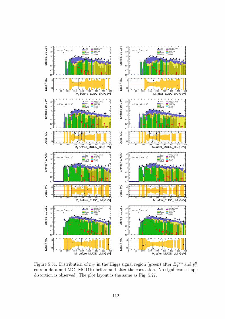
Ent
ries
/ 10
GeV
-310
-210
-110
1
10
210
310-1
Ldt =4.7 fb∫= 7 TeV, s
Data stat)⊕SM (sys WW γWZ/ZZ/Wtt Single Top
Z+jets W+jetsc/cb b H [125]
before_ELEC_BK [GeV]TM0 50 100 150 200 250 300 350 400D
ata
/ MC
0.8
1
1.2
Ent
ries
/ 10
GeV
-310
-210
-110
1
10
210
310-1
Ldt =4.7 fb∫= 7 TeV, s
Data stat)⊕SM (sys WW γWZ/ZZ/Wtt Single Top
Z+jets W+jetsc/cb b H [125]
after_ELEC_BK [GeV]TM0 50 100 150 200 250 300 350 400D
ata
/ MC
0.8
1
1.2
Ent
ries
/ 10
GeV
-310
-210
-110
1
10
210
310-1
Ldt =4.7 fb∫= 7 TeV, s
Data stat)⊕SM (sys WW γWZ/ZZ/Wtt Single Top
Z+jets W+jetsc/cb b H [125]
before_MUON_BK [GeV]TM0 50 100 150 200 250 300 350 400D
ata
/ MC
0.8
1
1.2
Ent
ries
/ 10
GeV
-310
-210
-110
1
10
210
310-1
Ldt =4.7 fb∫= 7 TeV, s
Data stat)⊕SM (sys WW γWZ/ZZ/Wtt Single Top
Z+jets W+jetsc/cb b H [125]
after_MUON_BK [GeV]TM0 50 100 150 200 250 300 350 400D
ata
/ MC
0.8
1
1.2
Ent
ries
/ 10
GeV
-310
-210
-110
1
10
210
310-1
Ldt =4.7 fb∫= 7 TeV, s
Data stat)⊕SM (sys WW γWZ/ZZ/Wtt Single Top
Z+jets W+jetsc/cb b H [125]
before_ELEC_LM [GeV]TM0 50 100 150 200 250 300 350 400D
ata
/ MC
0.8
1
1.2
Ent
ries
/ 10
GeV
-310
-210
-110
1
10
210
310-1
Ldt =4.7 fb∫= 7 TeV, s
Data stat)⊕SM (sys WW γWZ/ZZ/Wtt Single Top
Z+jets W+jetsc/cb b H [125]
after_ELEC_LM [GeV]TM0 50 100 150 200 250 300 350 400D
ata
/ MC
0.8
1
1.2
Ent
ries
/ 10
GeV
-310
-210
-110
1
10
210
310-1
Ldt =4.7 fb∫= 7 TeV, s
Data stat)⊕SM (sys WW γWZ/ZZ/Wtt Single Top
Z+jets W+jetsc/cb b H [125]
before_MUON_LM [GeV]TM0 50 100 150 200 250 300 350 400D
ata
/ MC
0.8
1
1.2
Ent
ries
/ 10
GeV
-310
-210
-110
1
10
210
310-1
Ldt =4.7 fb∫= 7 TeV, s
Data stat)⊕SM (sys WW γWZ/ZZ/Wtt Single Top
Z+jets W+jetsc/cb b H [125]
after_MUON_LM [GeV]TM0 50 100 150 200 250 300 350 400D
ata
/ MC
0.8
1
1.2
Figure 5.31: Distribution of mT in the Higgs signal region (green) after EmissT and pll
T
cuts in data and MC (MC11b) before and after the correction. No significant shapedistortion is observed. The plot layout is the same as Fig. 5.27.
112
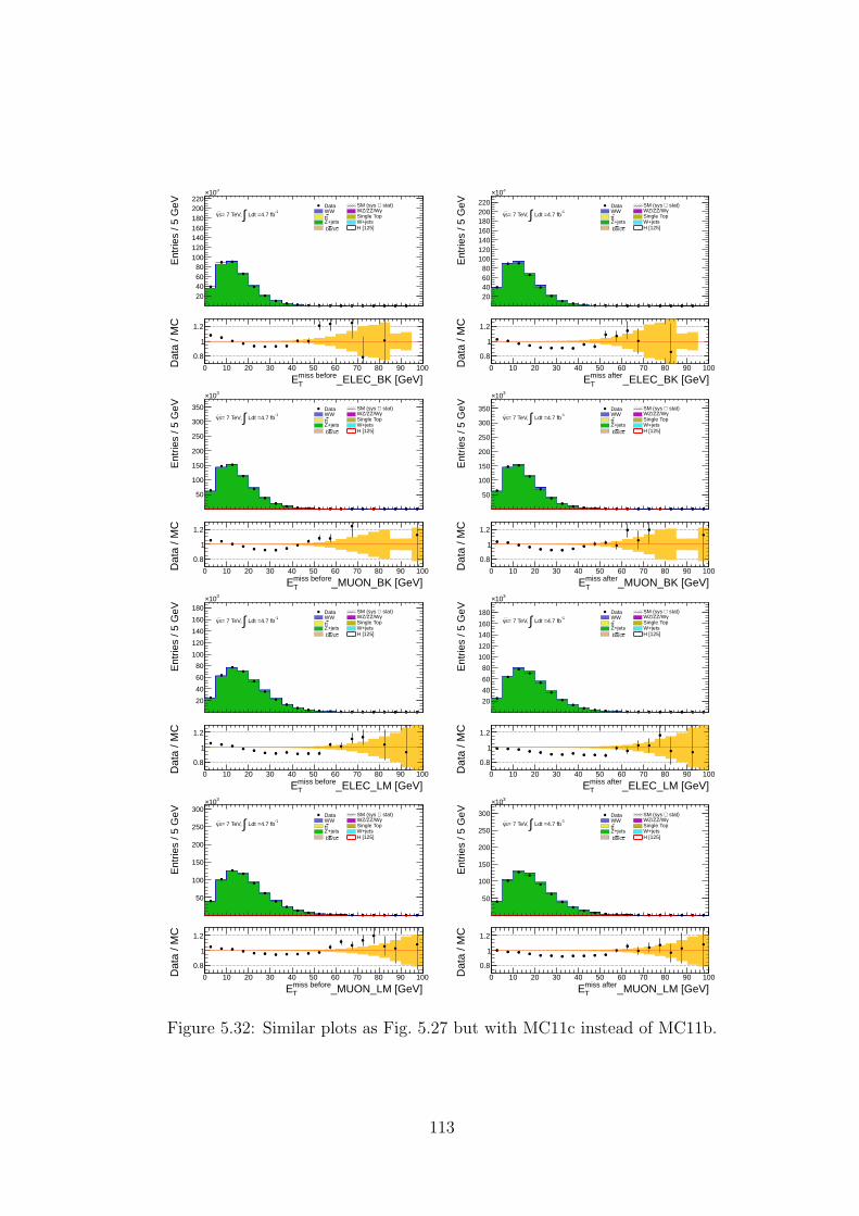
Ent
ries
/ 5 G
eV
20406080
100120140160180200220
310×
-1 Ldt =4.7 fb∫= 7 TeV, s
Data stat)⊕SM (sys WW γWZ/ZZ/Wtt Single Top
Z+jets W+jetsc/cb b H [125]
_ELEC_BK [GeV]miss beforeTE
0 10 20 30 40 50 60 70 80 90 100Dat
a / M
C
0.8
1
1.2
Ent
ries
/ 5 G
eV
20406080
100120140160180200220
310×
-1 Ldt =4.7 fb∫= 7 TeV, s
Data stat)⊕SM (sys WW γWZ/ZZ/Wtt Single Top
Z+jets W+jetsc/cb b H [125]
_ELEC_BK [GeV]miss afterTE
0 10 20 30 40 50 60 70 80 90 100Dat
a / M
C
0.8
1
1.2
Ent
ries
/ 5 G
eV
50
100
150
200
250
300
350
310×
-1 Ldt =4.7 fb∫= 7 TeV, s
Data stat)⊕SM (sys WW γWZ/ZZ/Wtt Single Top
Z+jets W+jetsc/cb b H [125]
_MUON_BK [GeV]miss beforeTE
0 10 20 30 40 50 60 70 80 90 100Dat
a / M
C
0.8
1
1.2
Ent
ries
/ 5 G
eV
50
100
150
200
250
300
350
310×
-1 Ldt =4.7 fb∫= 7 TeV, s
Data stat)⊕SM (sys WW γWZ/ZZ/Wtt Single Top
Z+jets W+jetsc/cb b H [125]
_MUON_BK [GeV]miss afterTE
0 10 20 30 40 50 60 70 80 90 100Dat
a / M
C
0.8
1
1.2
Ent
ries
/ 5 G
eV
20
40
60
80
100
120
140
160
180
310×
-1 Ldt =4.7 fb∫= 7 TeV, s
Data stat)⊕SM (sys WW γWZ/ZZ/Wtt Single Top
Z+jets W+jetsc/cb b H [125]
_ELEC_LM [GeV]miss beforeTE
0 10 20 30 40 50 60 70 80 90 100Dat
a / M
C
0.8
1
1.2
Ent
ries
/ 5 G
eV
20
40
60
80
100
120
140
160
180
310×
-1 Ldt =4.7 fb∫= 7 TeV, s
Data stat)⊕SM (sys WW γWZ/ZZ/Wtt Single Top
Z+jets W+jetsc/cb b H [125]
_ELEC_LM [GeV]miss afterTE
0 10 20 30 40 50 60 70 80 90 100Dat
a / M
C
0.8
1
1.2
Ent
ries
/ 5 G
eV
50
100
150
200
250
300
310×
-1 Ldt =4.7 fb∫= 7 TeV, s
Data stat)⊕SM (sys WW γWZ/ZZ/Wtt Single Top
Z+jets W+jetsc/cb b H [125]
_MUON_LM [GeV]miss beforeTE
0 10 20 30 40 50 60 70 80 90 100Dat
a / M
C
0.8
1
1.2
Ent
ries
/ 5 G
eV
50
100
150
200
250
300
310×
-1 Ldt =4.7 fb∫= 7 TeV, s
Data stat)⊕SM (sys WW γWZ/ZZ/Wtt Single Top
Z+jets W+jetsc/cb b H [125]
_MUON_LM [GeV]miss afterTE
0 10 20 30 40 50 60 70 80 90 100Dat
a / M
C
0.8
1
1.2
Figure 5.32: Similar plots as Fig. 5.27 but with MC11c instead of MC11b.
113
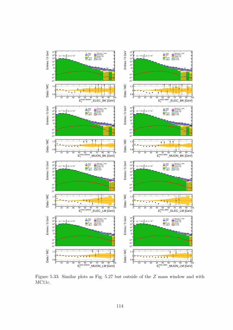
Ent
ries
/ 5 G
eV
-310
-210
-110
1
10
210
310
410
510
610
-1 Ldt =4.7 fb∫= 7 TeV, s
Data stat)⊕SM (sys WW γWZ/ZZ/Wtt Single Top
Z+jets W+jetsc/cb b H [125]
_ELEC_BK [GeV]miss beforeTE
0 10 20 30 40 50 60 70 80 90 100Dat
a / M
C
0.8
1
1.2
Ent
ries
/ 5 G
eV
-310
-210
-110
1
10
210
310
410
510
610-1
Ldt =4.7 fb∫= 7 TeV, s
Data stat)⊕SM (sys WW γWZ/ZZ/Wtt Single Top
Z+jets W+jetsc/cb b H [125]
_ELEC_BK [GeV]miss afterTE
0 10 20 30 40 50 60 70 80 90 100Dat
a / M
C
0.8
1
1.2
Ent
ries
/ 5 G
eV
-310
-210
-110
1
10
210
310
410
510
610-1
Ldt =4.7 fb∫= 7 TeV, s
Data stat)⊕SM (sys WW γWZ/ZZ/Wtt Single Top
Z+jets W+jetsc/cb b H [125]
_MUON_BK [GeV]miss beforeTE
0 10 20 30 40 50 60 70 80 90 100Dat
a / M
C
0.8
1
1.2
Ent
ries
/ 5 G
eV
-310
-210
-110
1
10
210
310
410
510
610-1
Ldt =4.7 fb∫= 7 TeV, s
Data stat)⊕SM (sys WW γWZ/ZZ/Wtt Single Top
Z+jets W+jetsc/cb b H [125]
_MUON_BK [GeV]miss afterTE
0 10 20 30 40 50 60 70 80 90 100Dat
a / M
C
0.8
1
1.2
Ent
ries
/ 5 G
eV
-310
-210
-110
1
10
210
310
410
510
610
-1 Ldt =4.7 fb∫= 7 TeV, s
Data stat)⊕SM (sys WW γWZ/ZZ/Wtt Single Top
Z+jets W+jetsc/cb b H [125]
_ELEC_LM [GeV]miss beforeTE
0 10 20 30 40 50 60 70 80 90 100Dat
a / M
C
0.8
1
1.2
Ent
ries
/ 5 G
eV
-310
-210
-110
1
10
210
310
410
510
610
-1 Ldt =4.7 fb∫= 7 TeV, s
Data stat)⊕SM (sys WW γWZ/ZZ/Wtt Single Top
Z+jets W+jetsc/cb b H [125]
_ELEC_LM [GeV]miss afterTE
0 10 20 30 40 50 60 70 80 90 100Dat
a / M
C
0.8
1
1.2
Ent
ries
/ 5 G
eV
-310
-210
-110
1
10
210
310
410
510
610-1
Ldt =4.7 fb∫= 7 TeV, s
Data stat)⊕SM (sys WW γWZ/ZZ/Wtt Single Top
Z+jets W+jetsc/cb b H [125]
_MUON_LM [GeV]miss beforeTE
0 10 20 30 40 50 60 70 80 90 100Dat
a / M
C
0.8
1
1.2
Ent
ries
/ 5 G
eV
-310
-210
-110
1
10
210
310
410
510
610-1
Ldt =4.7 fb∫= 7 TeV, s
Data stat)⊕SM (sys WW γWZ/ZZ/Wtt Single Top
Z+jets W+jetsc/cb b H [125]
_MUON_LM [GeV]miss afterTE
0 10 20 30 40 50 60 70 80 90 100Dat
a / M
C
0.8
1
1.2
Figure 5.33: Similar plots as Fig. 5.27 but outside of the Z mass window and withMC11c.
114
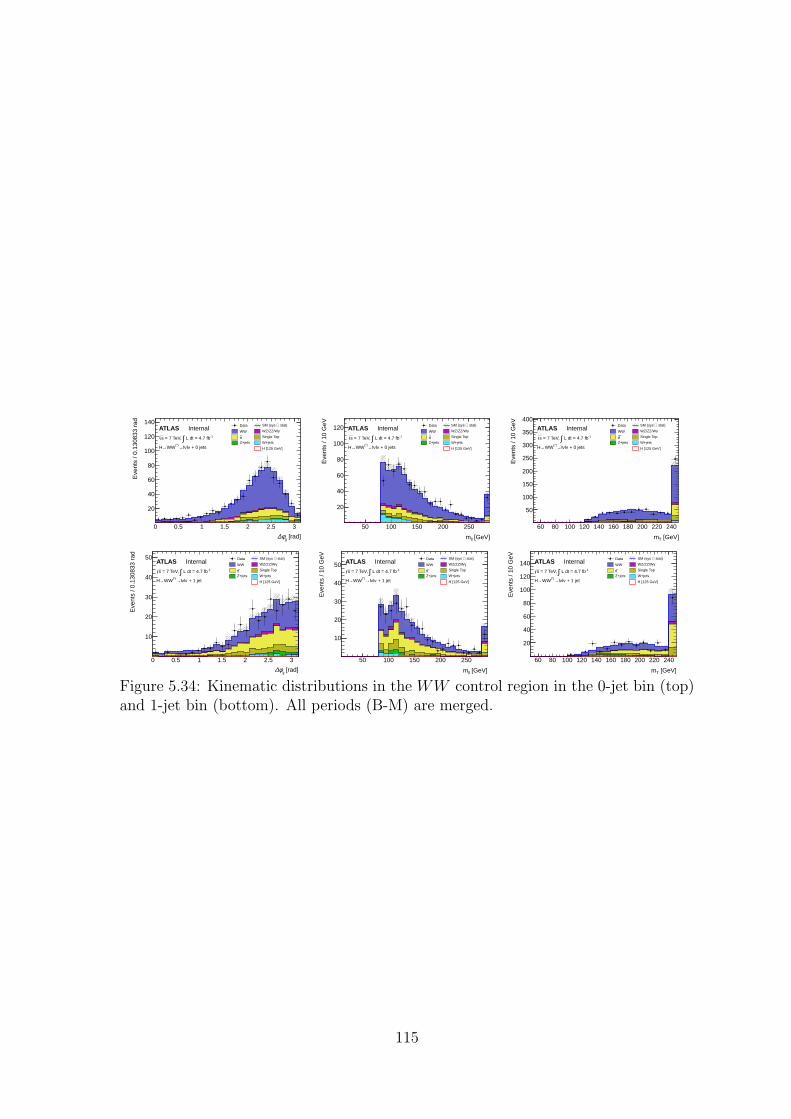
[rad]ll
φ∆0 0.5 1 1.5 2 2.5 3
Eve
nts
/ 0.1
3083
3 ra
d
20
40
60
80
100
120
140 Data stat)⊕ SM (sys
WW γ WZ/ZZ/W
t t Single Top
Z+jets W+jets
H [125 GeV]
ATLAS Internal-1 L dt = 4.7 fb∫ = 7 TeV, s
+ 0 jetsνlνl→(*)WW→H
[GeV]llm
50 100 150 200 250
Eve
nts
/ 10
GeV
20
40
60
80
100
120 Data stat)⊕ SM (sys
WW γ WZ/ZZ/W
t t Single Top
Z+jets W+jets
H [125 GeV]
ATLAS Internal-1 L dt = 4.7 fb∫ = 7 TeV, s
+ 0 jetsνlνl→(*)WW→H
[GeV]Tm
60 80 100 120 140 160 180 200 220 240
Eve
nts
/ 10
GeV
50
100
150
200
250
300
350
400 Data stat)⊕ SM (sys
WW γ WZ/ZZ/W
t t Single Top
Z+jets W+jets
H [125 GeV]
ATLAS Internal-1 L dt = 4.7 fb∫ = 7 TeV, s
+ 0 jetsνlνl→(*)WW→H
[rad]ll
φ∆0 0.5 1 1.5 2 2.5 3
Eve
nts
/ 0.1
3083
3 ra
d
10
20
30
40
50 Data stat)⊕ SM (sys
WW γ WZ/ZZ/W
t t Single Top
Z+jets W+jets
H [125 GeV]
ATLAS Internal-1 L dt = 4.7 fb∫ = 7 TeV, s
+ 1 jetνlνl→(*)WW→H
[GeV]llm
50 100 150 200 250
Eve
nts
/ 10
GeV
10
20
30
40
50 Data stat)⊕ SM (sys
WW γ WZ/ZZ/W
t t Single Top
Z+jets W+jets
H [125 GeV]
ATLAS Internal-1 L dt = 4.7 fb∫ = 7 TeV, s
+ 1 jetνlνl→(*)WW→H
[GeV]Tm
60 80 100 120 140 160 180 200 220 240
Eve
nts
/ 10
GeV
20
40
60
80
100
120
140 Data stat)⊕ SM (sys
WW γ WZ/ZZ/W
t t Single Top
Z+jets W+jets
H [125 GeV]
ATLAS Internal-1 L dt = 4.7 fb∫ = 7 TeV, s
+ 1 jetνlνl→(*)WW→H
Figure 5.34: Kinematic distributions in the WW control region in the 0-jet bin (top)and 1-jet bin (bottom). All periods (B-M) are merged.
115

116
Chapter 6
Results of Higgs Search in 2011
In this chapter, the statistical analysis basis for the Higgs discovery or exclusion isfirst introduced in Section 6.1. This is then applied in Section 6.2 to a search for aHiggs boson in a model with a fourth generation using part of the 2011 data and inSection 6.3 for the SM Higgs boson with the full 2011 data.
6.1 Statistical Analysis Basis
Once the data analysis is performed with the number of observed events and expectedbackground events, one needs to quantify for a signal (Higgs) discovery how largedeviation from the non Higgs hypothesis is and in case with no significant deviationif a Higgs mass can be excluded at a given confidence level. The statistical analysis isperformed using a binned likelihood function with the help of HistFactory frameworkand common RooStats tools [114, 115].
The likelihood function is constructed as the product of Poisson probability termsin each lepton flavor channel and jet bins, after all topological cuts except the mT
cut. In each region, the mT shape is taken into account. In the H + 0-jet (H +1-jet) signal regions, the mT shapes are divided into five (three) bins. The controlregions for WW and top (0-, 1-jet for WW and 1-, 2-jet for top) are introduced toextrapolate the background contribution. In the H + 2-jet signal region and controlregions, the mT is filled in only one bin due to the limited statistics. The bins insignal region are remapped to ensure enough statistics in each bin. In each channel(lepton or jet multiplicity), the likelihood function is defined as follows:
L(µ, b) = P (N |µs+ αb) × P (M |b) , (6.1)
where α = bexpSR /b
expCR is an extrapolation coefficient determined by MC, µ is the signal
(s) strength parameter (µ = 1 means the Standard Model Higgs prediction), and b isa free parameter representing the fitted background expectation in the control regionfor a given process (WW , top, etc), N is the measured number of events in the signalregion, while M is an auxiliary control region measurement. The data-driven back-ground estimation thus comes from maximising the likelihood over the parameters µ
117
and b. The variation on α due to systematic uncertainties is parametrized as follows:
L(µ, b, θ) = P (N |µs+ αb× να(θ)) × P (M |b) , (6.2)
in which να(θ) is the parameterised response to α, θ is the nuisance parameter, whichcan be constrained by a Gaussian function: N(θ|θ), representing an auxiliary measure-ment θ related to the nuisance parameter θ. Thus the whole model can be expressedas:
L(µ, ~θ) = {∏
l=B-K,L-M
∏
k=ee,eµ,µµ
Njets∏
j=0
Nbins∏
i=1
P (Nijkl|µsijkl +
Nbg∑
m
bijklm)} × {Nθ∏
i=1
N(θ|θ)} ,
(6.3)in which the final likelihood function is the product of likelihood in two different dataperiods B-K and L-M, all lepton channels, jet bins and mT bins.
The constraints on the numbers of background events for different processes aresummarised here.
Standard Model WW : For the low mass selections in the 0- and 1-jet channels,the normalization is constrained from a control region (obtained from the signalregion by removing the ∆φll requirement and replacing the mll upper boundwith a lower bound mll > 80GeV (mll > mZ + 15 GeV) for the eµ (ee and µµ)final states), two nuisance parameters are set for 0- and 1-jet bins. For 2-jetbin, the normalization is taken from Monte Carlo predictions.
tt + single top: In the 0-jet channel, Monte Carlo is used along with a data-drivennormalisation factor that corrects the jet veto efficiency with additional system-atics on the normalisation factor. In the 1- and 2-jet channels, the normalizationis constrained from a control region (obtained from the signal region definitionby reversing the b-jet veto and removing the requirements on ∆φll and mll).There are two separate nuisance parameters for the 1- and 2-jet normalizations.
Z/γ∗+jets: A data-driven method is used to determine the normalization in thesignal region as well as the contamination in the control regions. In the signalregion the shape is taken from Monte Carlo.
W+jets: A data-driven method is used to determine both the normalization andthe shape. There is a systematic uncertainty on the fake rate. Such uncertaintyaffects both the normalization and shape.
WZ/ZZ/Wγ: These backgrounds are taken from Monte Carlo.
Therefore the numbers of background events are constrained by two control regions.They are SMWW and top, presented in the Poisson distribution and a series Gaussianconstraint terms.
118
When the likelihood function is constructed, a test statistic is defined as the ratioof log likelihood with the one side constraint:
qµ =
−2 ln L(µ,ˆθ(µ))
L(0,ˆθ(0))
µ < 0,
−2 ln L(µ,ˆθ(µ))
L(µ,θ)0 ≤ µ ≤ µ,
0 µ > µ ,
(6.4)
in which the µ and θ are the value obtained by maximizing the L and theˆθ comes
from maximizing the L with a specific µ. The p-values of pµ and pb are derived from
the sampling distributions f(qµ|µ, θµ) and f(qµ|0, θ0), respectively:
pµ =
∫ ∞
qµ,obs
f(qµ|µ, θµ)dqµ , pb =
∫ qµ,obs
∞
f(qµ|0, θ0)dqµ . (6.5)
In the Higgs discovery case, the p value is defined under the background-only hypoth-esis with a different constraint µ > 0:
p0 =
∫ ∞
q0,obs
f(q0|0, θ0)dq0 . (6.6)
And it can be interpreted as statistical significance Z:
Z = Φ−1(1 − p0) . (6.7)
When Z is larger than 3 it is possible to claim an evidence or 5 for discovery. In theexclusion case, the CLs method is used and defined as:
CLs =pµ
1 − pb
. (6.8)
The upper limit is usually set at 95% so that CLs=0.05. For a given µ, if the observedCLs is smaller than 0.05 and the µ is smaller than 1, it is said that the Higgs bosonwith such mass is excluded. It is CPU time consuming to calculate the p value tosatisfy a given CLs, so an asymptotic approximation is introduced to simplify thecomputation [113].
6.2 Results for a Fourth generation Higgs Search
The SM is known to have three families of charged and neutral fermions. Thereis however no upper limit on the number of fermion familities. A fourth familycould in fact be the key to many unsolved puzzles, such as the hierarchies of thefermion mass spectrum including neutrino masses and mixing, electroweak symmetrybreaking, baryogenesis, and a variety of interesting phenomena in CP and flavorphysics [23, 24, 25, 26, 27].
119
As shown in Eq. 1.30, the interaction strength of the Higgs to a fermion is propor-tional to the fermion mass in Yukawa couplings. Thus, the production cross sectionis significantly enhanced by including the contribution of fourth generation quarkswith heavy masses [22]. Fourth family leptons and quarks have been searched forpreviously by the LEP and Tevtran experiments and now by the LHC experiments.The most stringent lower mass limits at 95% CL of fourth family leptons and quarksare given in [16, 19, 20, 28, 29, 30, 31]:
mν4 > 80.5 − 101.5 GeV, (6.9)
ml4 > 100.8 GeV , (6.10)
mb4 > 611 GeV , (6.11)
mt4 > 557 GeV . (6.12)
In the SM, the dominant Higgs production process is the gluon-gluon fusion pro-cess where gluons from the colliding beams couple to a heavy quark loop from whichthe Higgs boson is emitted (see Fig. 1.3). The production cross section can be ex-pressed as:
σ(pp→ HX) = Γ(H → gg)π2
8m3H
τH
∫ 1
τH
dx
xg(x,m2
H)g(τH/x,m2H) , (6.13)
with
Γ(H → gg) =GFm
3H
36√
2π
[
αs(m2H)
π
]2
|I|2 , I =∑
q
Iq , (6.14)
in which g(x,Q2) is the gluon distribution evaluated at x and Q2, GF (αs) is the Fermi(strong) coupling constant. The quantity Iq is given in terms of λq = m2
q/m2H :
Iq = 3[2λq + λq(4λq − 1)f(λq)] , (6.15)
where
f(λq) =
{ −2{sin−1 1
2√
λq
}2, for λq >14,
12(ln η+
η−)2 − π2
2− iπ η+
η−, for λq <
14,
(6.16)
with η± = 12±√
14− λq. When the quark is very heavy, with λq ≫ 1, Iq → 1, otherwise
if the quark is very light, λq ≪ 1, Iq → 0, so the contribution from the heaviest quarkis dominant. When the fourth generation is included, the Higgs production corsssection is enhanced over that of the SM by a factor:
RSM4/SMσ(gg→H) ≡
σ(gg → H)SM4
σ(gg → H)SM
=|Ib + It + It4 + Id4|2
|Ib + It|2. (6.17)
The dependence of the enhancement factor as a function of the Higgs boson massmH is shown in Fig. 6.1 [22] (left) for two different md4 values: infinite mass (inpractice a value of 10 TeV is chosen) and 400 GeV. The t4 mass is fixed as [32]:
mt4 = md4 + 50 + 20 × ln(mH
115[GeV]), (6.18)
120
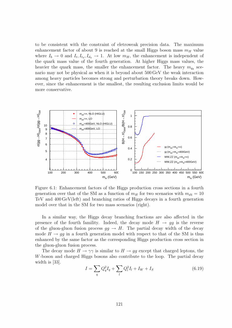
to be consistent with the constraint of eletroweak precision data. The maximumenhancement factor of about 9 is reached at the small Higgs boson mass mH valuewhere Ib → 0 and It, It4 , Id4 → 1. At low mH , the enhancement is independent ofthe quark mass value of the fourth generation. At higher Higgs mass values, theheavier the quark mass, the smaller the enhancement factor. The heavy mq4 sce-nario may not be physical as when it is beyond about 500 GeV the weak interactionamong heavy particles becomes strong and perturbation theory breaks down. How-ever, since the enhancement is the smallest, the resulting exclusion limits would bemore conservative.
4
5
6
7
8
910
100 200 300 400 500 600
mH (GeV)
σ(gg
→H
) SM
4/σ(
gg→
H) S
M
md4=∞, NLO (HIGLU)
md4=∞, LO
md4=400GeV, NLO (HIGLU)
md4=400GeV, LO
0
0.2
0.4
0.6
0.8
1
100 150 200 250 300 350 400 450 500 550 600
mH (GeV)
B(H
→X
) SM
4/B
(H→
X) S
M
γγ (md4=ml4=∞)
γγ (md4=ml4=400GeV)
WW,ZZ (md4=ml4=∞)
WW,ZZ (md4=ml4=400GeV)
Figure 6.1: Enhancement factors of the Higgs production cross sections in a fourthgeneration over that of the SM as a function of mH for two scenarios with md4 = 10TeV and 400 GeV(left) and branching ratios of Higgs decays in a fourth generationmodel over that in the SM for two mass scenarios (right).
In a similar way, the Higgs decay branching fractions are also affected in thepresence of the fourth famility. Indeed, the decay mode H → gg is the reverseof the gluon-gluon fusion process gg → H. The partial decay width of the decaymode H → gg in a fourth generation model with respect to that of the SM is thusenhanced by the same factor as the corresponding Higgs production cross section inthe gluon-gluon fusion process.
The decay mode H → γγ is similar to H → gg except that charged leptons, theW -boson and charged Higgs bosons also contribute to the loop. The partial decaywidth is [33].
I =∑
q
Q2qIq +
∑
l
Q2l Il + IW + IS (6.19)
121
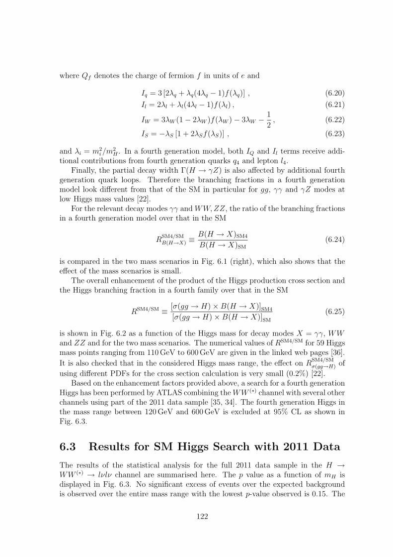
where Qf denotes the charge of fermion f in units of e and
Iq = 3 [2λq + λq(4λq − 1)f(λq)] , (6.20)
Il = 2λl + λl(4λl − 1)f(λl) , (6.21)
IW = 3λW (1 − 2λW )f(λW ) − 3λW − 1
2, (6.22)
IS = −λS [1 + 2λSf(λS)] , (6.23)
and λi = m2i /m
2H . In a fourth generation model, both IQ and Il terms receive addi-
tional contributions from fourth generation quarks q4 and lepton l4.Finally, the partial decay width Γ(H → γZ) is also affected by additional fourth
generation quark loops. Therefore the branching fractions in a fourth generationmodel look different from that of the SM in particular for gg, γγ and γZ modes atlow Higgs mass values [22].
For the relevant decay modes γγ andWW,ZZ, the ratio of the branching fractionsin a fourth generation model over that in the SM
RSM4/SMB(H→X) ≡
B(H → X)SM4
B(H → X)SM
(6.24)
is compared in the two mass scenarios in Fig. 6.1 (right), which also shows that theeffect of the mass scenarios is small.
The overall enhancement of the product of the Higgs production cross section andthe Higgs branching fraction in a fourth family over that in the SM
RSM4/SM ≡ [σ(gg → H) ×B(H → X)]SM4
[σ(gg → H) ×B(H → X)]SM
(6.25)
is shown in Fig. 6.2 as a function of the Higgs mass for decay modes X = γγ, WWand ZZ and for the two mass scenarios. The numerical values of RSM4/SM for 59 Higgsmass points ranging from 110 GeV to 600 GeV are given in the linked web pages [36].
It is also checked that in the considered Higgs mass range, the effect on RSM4/SMσ(gg→H) of
using different PDFs for the cross section calculation is very small (0.2%) [22].Based on the enhancement factors provided above, a search for a fourth generation
Higgs has been performed by ATLAS combining theWW (∗) channel with several otherchannels using part of the 2011 data sample [35, 34]. The fourth generation Higgs inthe mass range between 120 GeV and 600 GeV is excluded at 95% CL as shown inFig. 6.3.
6.3 Results for SM Higgs Search with 2011 Data
The results of the statistical analysis for the full 2011 data sample in the H →WW (∗) → lνlν channel are summarised here. The p value as a function of mH isdisplayed in Fig. 6.3. No significant excess of events over the expected backgroundis observed over the entire mass range with the lowest p-value observed is 0.15. The
122
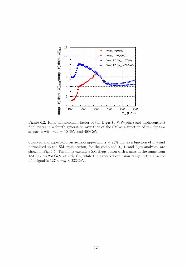
0
2
4
6
8
10
12
100 200 300 400 500 600
mH (GeV)(σ(g
g→H
)xB
(H→
X))
SM
4/(σ
(gg→
H)x
B(H
→X
))S
M
γγ (md4=10TeV)
γγ (md4=400GeV)
WW, ZZ (md4=10TeV)
WW, ZZ (md4=400GeV)
Figure 6.2: Final enhancement factor of the Higgs to WW(blue) and diphoton(red)final states in a fourth generation over that of the SM as a function of mH for twoscenarios with md4 = 10 TeV and 400 GeV.
observed and expected cross section upper limits at 95% CL, as a function of mH andnormalised to the SM cross section, for the combined 0-, 1- and 2-jet analyses, areshown in Fig. 6.5. The limits exclude a SM Higgs boson with a mass in the range from133 GeV to 261GeV at 95% CL, while the expected exclusion range in the absenceof a signal is 127 < mH < 233 GeV.
123
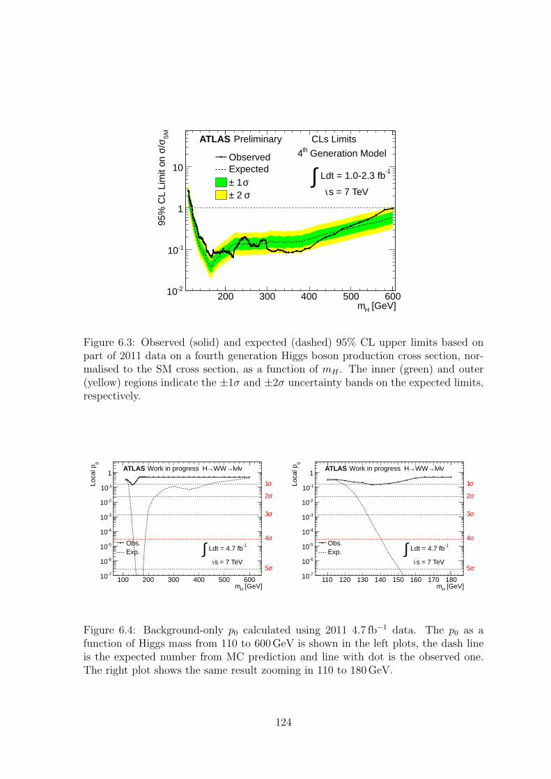
[GeV]Hm200 300 400 500 600
SM
σ/σ95
% C
L Li
mit
on
-210
-110
1
10ObservedExpected
σ 1 ±σ 2 ±
ATLAS Preliminary
-1 Ldt = 1.0-2.3 fb∫ = 7 TeVs
CLs Limits
Generation Modelth4
Figure 6.3: Observed (solid) and expected (dashed) 95% CL upper limits based onpart of 2011 data on a fourth generation Higgs boson production cross section, nor-malised to the SM cross section, as a function of mH . The inner (green) and outer(yellow) regions indicate the ±1σ and ±2σ uncertainty bands on the expected limits,respectively.
[GeV]Hm100 200 300 400 500 600
0Lo
cal p
-710
-610
-510
-410
-310
-210
-110
1
Obs. Exp.
σ1
σ2
σ3
σ4
σ5 = 7 TeVs
-1 Ldt = 4.7 fb∫
ATLAS Work in progress νlνl→WW→H
[GeV]Hm110 120 130 140 150 160 170 180
0Lo
cal p
-710
-610
-510
-410
-310
-210
-110
1
Obs. Exp.
σ1
σ2
σ3
σ4
σ5 = 7 TeVs
-1 Ldt = 4.7 fb∫
ATLAS Work in progress νlνl→WW→H
Figure 6.4: Background-only p0 calculated using 2011 4.7 fb−1 data. The p0 as afunction of Higgs mass from 110 to 600 GeV is shown in the left plots, the dash lineis the expected number from MC prediction and line with dot is the observed one.The right plot shows the same result zooming in 110 to 180 GeV.
124
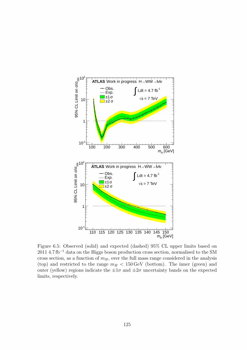
[GeV]Hm100 200 300 400 500 600
SM
σ/σ95
% C
L Li
mit
on
-110
1
10
210
Obs. Exp.
σ1 ±σ2 ±
= 7 TeVs
-1 Ldt = 4.7 fb∫ATLAS Work in progress νlνl→WW→H
[GeV]Hm110 115 120 125 130 135 140 145 150
SM
σ/σ95
% C
L Li
mit
on
-110
1
10
210
Obs. Exp.
σ1 ±σ2 ±
= 7 TeVs
-1 Ldt = 4.7 fb∫ATLAS Work in progress νlνl→WW→H
Figure 6.5: Observed (solid) and expected (dashed) 95% CL upper limits based on2011 4.7 fb−1 data on the Higgs boson production cross section, normalised to the SMcross section, as a function of mH , over the full mass range considered in the analysis(top) and restricted to the range mH < 150 GeV (bottom). The inner (green) andouter (yellow) regions indicate the ±1σ and ±2σ uncertainty bands on the expectedlimits, respectively.
125

126
Chapter 7
Results of Higgs Search in 2012
The analysis of 2012 data (sample used for the ICHEP2012 conference) correspond-ing to an integrated luminosity of 5.8 fb−1 follows closely the analysis of the 2011data [117]. Nevertheless there are a number of differences and new features which aredescribed in Section 7.1.
7.1 Improvements and New Features in 2012
In 2012, the center-of-mass energy has been increased from 7 TeV to 8TeV. By theend of June, a sample with an integrated luminosity exceeding that of 2011 has beentaken by the ATLAS detector and analyzed [116] with the final results published [118].In 2011, the average number of interactions per bunch crossing was around 10. In2012, the average is increased to around 20 so that the analysis is more challengingand has to be improved to reduce its dependence on the pile up effects.
The first change is on the trigger, which has been updated to cope with theincreasing interating rate, as described in Tab 7.1.
2011 ee channel µµ channel eµ channel
B - I EF e20 medium EF mu18 MG EF e20 medium || EF mu18 MGJ EF e20 medium EF mu18 MG medium EF e20 medium || EF mu18 MG mediumK EF e22 medium EF mu18 MG medium EF e22 medium || EF mu18 MG mediumL - M EF e22vh medium1 EF mu18 MG medium EF e22vh medium1 || EF mu18 MG medium
2012 ee EF e24vhi medium1 || EF e60 medium12012 µµ EF mu24i tight || EF mu36 tight2012 eµ & µe EF e24vhi medium1 || EF e60 medium1 || EF mu24i tight || EF mu36 tight
Table 7.1: Proposed trigger setup for 2011 periods (upper table) and 2012 run (lowertable).
The next main modification in 2012 is on the lepton selection [135]:
• The topological cluster based calorimeter isolation on electrons is used insteadof the cell based algorithm in 2011 to reduce the pile up dependence.
127
• The track isolation of electrons is improved due to the change of the lowerthreshold for each tracks which are used for the calculation of the track isolationfrom 900 MeV in 2011 to 400MeV in 2012.
• The electron track impact parameter resolutions are significantly improved in2012 due to the new Gaussian Sum Fitter (GSF) algorithm [106].
• Pile up correction is applied on muon isolation.
• The η range of muon is extended from 2.4 to to 2.5.
All of the impact parameter cuts are reoptimzed. The modified cuts for muons andelectrons are shown in Tabs. 7.2 and 7.3.
2011 Cut 2012 Cutpile up corrected etcone30/pT < 0.14 topo etconecor30/pT < 0.16ptcone30/pT < 0.13 ptcone30/pT < 0.12 for 15 − 25GeV
ptcone30/pT < 0.16 for > 25GeVd0(sig) < 10 d0(sig) < 3.0|z0|(w.r.t.PV) < 1 mm |z0 sin θ| < 0.4 mm
Table 7.2: Electron isolation and impact parameter cuts.
2011 Cut 2012 Cutmu staco etcone30/pT < 0.14 etconecor30/pT < 0.014 × pT − 0.15
&& etconecor30/pT < 0.20mu staco ptcone30/pT < 0.15 ptcone30/pT < 0.01 × pT − 0.105
&& ptcone30/pT < 0.15d0(sig) < 3 d0(sig) < 3|z0|(w.r.t.PV) < 1 mm |z0 sin θ| < 1.0 mm
Table 7.3: Muon isolation and impact parameter cuts.
Due to the increased pile up interactions, the calorimeter based EmissT has seen
it resolution degraded such that for a same EmissT cut, the Z/DY background has
significantly increased for the same flavour channels. For this reason, for the firstresults reported in [118], the analysis is limited to the eµ channel which has thedominant sensivity. To improve the search sensitivity in the analysis of the 2012data, the channel has been splitted into two independent channels: eµ and µe wherethe first lepton stands for the leading lepton.
The jets selection is slightly changed. The pT threshold remains 25 GeV for|η| < 2.5 and is raised to 30 GeV for |η| > 2.5. The JVF threshold is changedfrom 0.75 to 0.5 to reduce the pile up dependence, shown in Fig 7.1. The b-taggingalgorithm has also been changed from a combined neutral network based one (Jet-FitterCombNN [119]) at 80% working point to a multivariate based one (MV1 [120])at 85% working point.
128
PVN5 10 15 20 25 30
> 2
0 G
eV)
LC TJe
t Mul
tiplic
ity (
p
0.5
1
1.5
2
2.5
3
3.5
4raw
offset correctedtrk-jet confirmed
JVF > 0.75JVF > 0.50JVF > 0.25
LC R=0.4tAnti-k| < 1.9η|
HS Jets> = 20µ<
PVN5 10 15 20 25 30 35 40 45
> 2
0 G
eV)
LC TJe
t Mul
tiplic
ity (
p
0.5
1
1.5
2
2.5
3
3.5
4raw
offset correctedtrk-jet confirmed
JVF > 0.75JVF > 0.50JVF > 0.25
LC R=0.4tAnti-k| < 1.9η|
HS Jets> = 40µ<
Figure 7.1: The JV F efficiency as a function of NPV for calibrated LC(local clusterweighting)+JES jets for < µ >= 20 (left) and < µ >= 40 (right) running conditions.
The main new feature in the analysis of 2012 is that the signal region has beenblinded with the following cuts:
• ∆φll < 1.8 ,
• mll < 50GeV ,
• 82.5 < mT < 140 GeV ,
• b-jet veto .
Thousands of kinematic distributions have been compared between data and thetotal SM background contributions derived either with the data-driven methods orwith data-validated MC predictions in different background control regions. Goodagreement has been observed in essentially all the distributions. One example isshown in Fig. 7.2 for the mT distribution in the WW 0-jet control region for the eµand µe channels. The KS prob shown on the plots is Kolmogorov-Smirnov probability,which describes the agreement between data and MC prediction. If the probabilityis close to one it means that these two distributions are compatible [121]. Figure 7.3shows the data and MC comparison of mT in top control region in which one of thejets must be b-tagged.
When the blinded analysis is approved by the Higgs working group, the signalregion is unblinded. Figure 7.4 shows the mT distribution in the signal region for 0-jet analysis, in which a significant excess over the background contribution observedin both the eµ and µe channels.
129
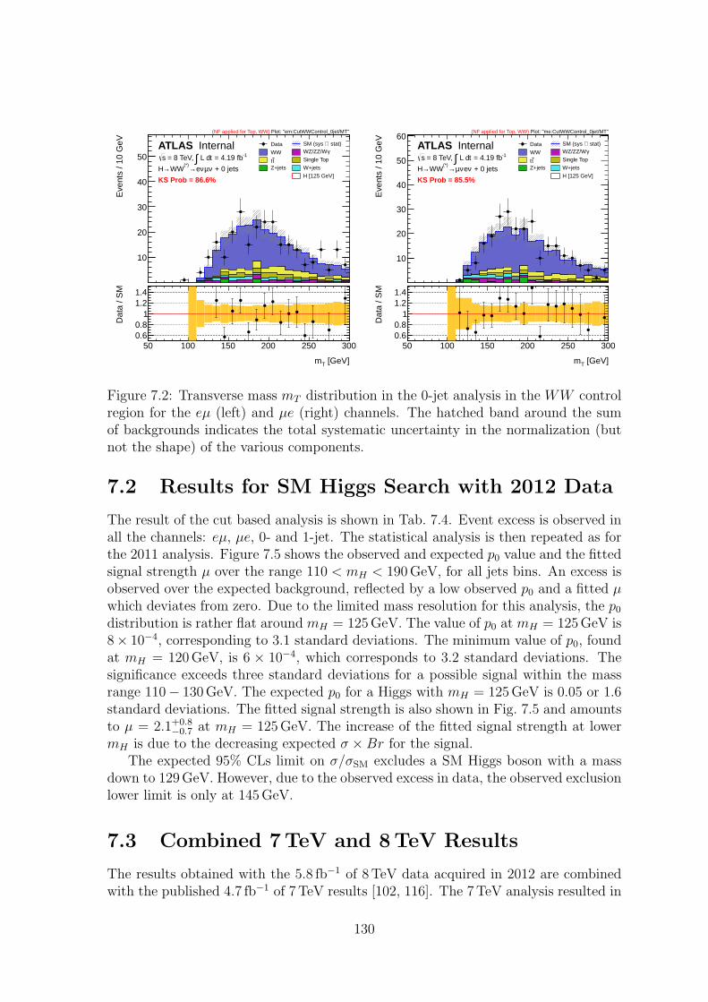
Eve
nts
/ 10
GeV
10
20
30
40
50
Data stat)⊕ SM (sys
WW γ WZ/ZZ/W
t t Single Top
Z+jets W+jets H [125 GeV]
ATLAS Internal-1 = 4.19 fbt L d∫ = 8 TeV, s
+ 0 jetsνµνe→(*)WW→H
Plot: "em:CutWWControl_0jet/MT"(NF applied for Top, WW)
KS Prob = 86.6%
[GeV]Tm
50 100 150 200 250 300
Dat
a / S
M
0.60.8
11.21.4
Eve
nts
/ 10
GeV
10
20
30
40
50
60 Data stat)⊕ SM (sys
WW γ WZ/ZZ/W
t t Single Top
Z+jets W+jets H [125 GeV]
ATLAS Internal-1 = 4.19 fbt L d∫ = 8 TeV, s
+ 0 jetsνeνµ→(*)WW→H
Plot: "me:CutWWControl_0jet/MT"(NF applied for Top, WW)
KS Prob = 85.5%
[GeV]Tm
50 100 150 200 250 300
Dat
a / S
M
0.60.8
11.21.4
Figure 7.2: Transverse mass mT distribution in the 0-jet analysis in the WW controlregion for the eµ (left) and µe (right) channels. The hatched band around the sumof backgrounds indicates the total systematic uncertainty in the normalization (butnot the shape) of the various components.
7.2 Results for SM Higgs Search with 2012 Data
The result of the cut based analysis is shown in Tab. 7.4. Event excess is observed inall the channels: eµ, µe, 0- and 1-jet. The statistical analysis is then repeated as forthe 2011 analysis. Figure 7.5 shows the observed and expected p0 value and the fittedsignal strength µ over the range 110 < mH < 190 GeV, for all jets bins. An excess isobserved over the expected background, reflected by a low observed p0 and a fitted µwhich deviates from zero. Due to the limited mass resolution for this analysis, the p0
distribution is rather flat around mH = 125 GeV. The value of p0 at mH = 125 GeV is8× 10−4, corresponding to 3.1 standard deviations. The minimum value of p0, foundat mH = 120 GeV, is 6 × 10⁻⁴, which corresponds to 3.2 standard deviations. Thesignificance exceeds three standard deviations for a possible signal within the massrange 110− 130 GeV. The expected p0 for a Higgs with mH = 125 GeV is 0.05 or 1.6standard deviations. The fitted signal strength is also shown in Fig. 7.5 and amountsto µ = 2.1+0.8
−0.7 at mH = 125 GeV. The increase of the fitted signal strength at lowermH is due to the decreasing expected σ ×Br for the signal.
The expected 95% CLs limit on σ/σSM excludes a SM Higgs boson with a massdown to 129 GeV. However, due to the observed excess in data, the observed exclusionlower limit is only at 145 GeV.
7.3 Combined 7TeV and 8TeV Results
The results obtained with the 5.8 fb−1 of 8 TeV data acquired in 2012 are combinedwith the published 4.7 fb−1 of 7 TeV results [102, 116]. The 7 TeV analysis resulted in
130
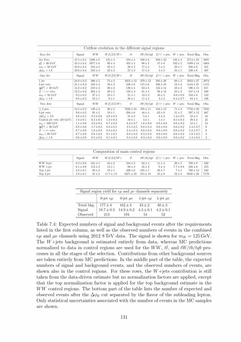
Cutflow evolution in the different signal regions
Zero Jet Signal WW WZ/ZZ/Wγ tt tW/tb/tqb Z/γ∗ + jets W + jets Total Bkg. Obs.
Jet Veto 47.5± 0.4 1308± 9 125± 4 184± 4 109± 6 850± 32 138± 4 2714± 34 2691pℓℓ
T > 30 GeV 43.4± 0.4 1077± 8 99± 4 165± 4 98± 5 47± 8 102± 2 1589± 14 1664mℓℓ < 50 GeV 34.9± 0.4 244± 4 33± 2 28± 2 17± 2 5± 2 29± 1 356± 6 421∆φℓℓ < 1.8 33.6± 0.4 234± 4 32± 2 27± 2 17± 2 4± 2 25± 1 339± 6 407
One Jet Signal WW WZ/ZZ/Wγ tt tW/tb/tqb Z/γ∗ + jets W + jets Total Bkg. Obs.
1 jet 24.9± 0.3 396± 5 74± 3 1652± 12 479± 12 283± 20 68± 3 2953± 27 2874b-jet veto 21.1± 0.3 334± 4 56± 2 349± 6 115± 6 236± 18 53± 2 1144± 21 1115|ptot
T | < 30 GeV 12.2± 0.2 210± 3 30± 2 139± 4 63± 5 124± 14 23± 2 590± 15 611Z → ττ veto 12.2± 0.2 204± 3 29± 2 133± 3 61± 5 98± 12 23± 2 547± 14 580mℓℓ < 50 GeV 9.2± 0.2 37± 1 10± 1 21± 1 12± 2 16± 5 8.0± 0.9 104± 6 122∆φℓℓ < 1.8 8.6± 0.2 34± 1 9± 1 20± 1 11± 2 3± 2 6.4± 0.7 84± 4 106
Two Jets Signal WW WZ/ZZ/Wγ tt tW/tb/tqb Z/γ∗ + jets W + jets Total Bkg. Obs.
≥ 2 jets 14.5± 0.2 139± 3 30± 2 7039± 24 376± 11 104± 12 71± 4 7759± 29 7845b-jet veto 9.6± 0.2 95± 2 19± 1 356± 6 44± 4 62± 9 21± 2 597± 12 667|∆Yjj| > 3.8 2.0± 0.1 8.3± 0.6 2.0± 0.4 31± 2 5± 1 4± 2 1.4± 0.5 52± 3 44Central jet veto (20 GeV) 1.6± 0.1 6.5± 0.5 1.3± 0.3 16± 1 4± 1 1± 1 0.5± 0.3 29± 2 22mjj > 500 GeV 1.1± 0.0 3.2± 0.4 0.7± 0.2 6.2± 0.7 1.8± 0.6 0.0± 0.0 0.0± 0.2 12± 1 13|ptot
T | < 30 GeV 0.8± 0.0 1.7± 0.3 0.3± 0.1 2.5± 0.5 0.8± 0.4 0.0± 0.0 0.0± 0.2 5.4± 0.7 6Z → ττ veto 0.7± 0.0 1.8± 0.3 0.3± 0.1 2.4± 0.4 0.8± 0.4 0.0± 0.0 0.0± 0.2 5.2± 0.7 6mℓℓ < 80 GeV 0.7± 0.0 0.6± 0.2 0.1± 0.1 0.8± 0.3 0.3± 0.2 0.0± 0.0 0.0± 0.2 1.9± 0.5 3∆φℓℓ < 1.8 0.6± 0.0 0.5± 0.2 0.1± 0.1 0.5± 0.3 0.3± 0.2 0.0± 0.0 0.0± 0.2 1.4± 0.4 2
Composition of main control regions
Signal WW WZ/ZZ/Wγ tt tW/tb/tqb Z/γ∗ + jets W + jets Total Bkg. Obs.
WW 0-jet 0.3± 0.0 531± 5 43± 2 104± 3 62± 4 11± 4 38± 1 789± 9 820WW 1-jet 0.1± 0.0 112± 3 13± 1 80± 3 34± 3 9± 4 7.7± 0.8 256± 6 255Top 1-jet 2.2± 0.1 39± 2 10± 1 489± 6 195± 7 28± 7 7± 1 768± 12 840Top 2-jet 4.9± 0.1 45± 2 11.7± 1.0 6371± 23 315± 10 45± 8 52± 3 6840± 26 7178
Signal region yield for eµ and µe channels separately
0-jet eµ 0-jet µe 1-jet eµ 1-jet µe
Total bkg. 177± 4 162± 4 43± 2 40± 3Signal 18.7± 0.3 14.9± 0.2 4.3± 0.1 4.2± 0.1Observed 213 194 54 52
Table 7.4: Expected numbers of signal and background events after the requirementslisted in the first column, as well as the observed numbers of events in the combinedeµ and µe channels using 2012 8 TeV data. The signal is shown for mH = 125 GeV.The W+jets background is estimated entirely from data, whereas MC predictionsnormalized to data in control regions are used for the WW , tt, and tW/tb/tqb pro-cesses in all the stages of the selection. Contributions from other background sourcesare taken entirely from MC predictions. In the middle part of the table, the expectednumbers of signal and background events, and the observed numbers of events, areshown also in the control regions. For these rows, the W+jets contribution is stilltaken from the data-driven estimate but no normalization factors are applied, exceptthat the top normalization factor is applied for the top background estimate in theWW control regions. The bottom part of the table lists the number of expected andobserved events after the ∆φll cut separated by the flavor of the subleading lepton.Only statistical uncertainties associated with the number of events in the MC samplesare shown.
131
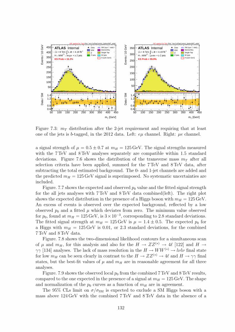
Eve
nts
/ 10
GeV
50
100
150
200
250
300
350
400
450 Data stat)⊕ SM (sys
WW γ WZ/ZZ/W
t t Single Top
Z+jets W+jets H [125 GeV]
ATLAS Internal-1 = 4.19 fbt L d∫ = 8 TeV, s
2 jets≥ + νµνe→(*)WW→H
Plot: "em:CutTopControl_2jetincl/MT_wide"(NF applied for Top)
KS Prob = 16.2%
[GeV]Tm
50 100 150 200 250 300 350 400 450
Dat
a / S
M
0.60.8
11.21.4
Eve
nts
/ 10
GeV
50
100
150
200
250
300
350 Data stat)⊕ SM (sys
WW γ WZ/ZZ/W
t t Single Top
Z+jets W+jets H [125 GeV]
ATLAS Internal-1 = 4.19 fbt L d∫ = 8 TeV, s
2 jets≥ + νeνµ→(*)WW→H
Plot: "me:CutTopControl_2jetincl/MT_wide"(NF applied for Top)
KS Prob = 99.9%
[GeV]Tm
50 100 150 200 250 300 350 400 450
Dat
a / S
M
0.60.8
11.21.4
Figure 7.3: mT distribution after the 2-jet requirement and requiring that at leastone of the jets is b-tagged, in the 2012 data. Left: eµ channel. Right: µe channel.
a signal strength of µ = 0.5 ± 0.7 at mH = 125 GeV. The signal strengths measuredwith the 7 TeV and 8 TeV analyses separately are compatible within 1.5 standarddeviations. Figure 7.6 shows the distribution of the transverse mass mT after allselection criteria have been applied, summed for the 7 TeV and 8 TeV data, aftersubtracting the total estimated background. The 0- and 1-jet channels are added andthe predicted mH = 125 GeV signal is superimposed. No systematic uncertainties areincluded.
Figure. 7.7 shows the expected and observed p0 value and the fitted signal strengthfor the all jets analyses with 7 TeV and 8 TeV data combined(left). The right plotshows the expected distribution in the presence of a Higgs boson with mH = 125 GeV.An excess of events is observed over the expected background, reflected by a lowobserved p0 and a fitted µ which deviates from zero. The minimum value observedfor p0, found at mH = 125 GeV, is 3×10⁻³, corresponding to 2.8 standard deviations.The fitted signal strength at mH = 125 GeV is µ = 1.4 ± 0.5. The expected p0 fora Higgs with mH = 125GeV is 0.01, or 2.3 standard deviations, for the combined7 TeV and 8 TeV data.
Figure. 7.8 shows the two-dimensional likelihood contours for a simultaneous scanof µ and mH , for this analysis and also for the H → ZZ(∗) → 4ℓ [122] and H →γγ [134] analyses. The lack of mass resolution in the H → WW (∗) → lνlν final statefor low mH can be seen clearly in contrast to the H → ZZ(∗) → 4ℓ and H → γγ finalstates, but the best-fit values of µ and mH are in reasonable agreement for all threeanalyses.
Figure. 7.9 shows the observed local p0 from the combined 7TeV and 8 TeV results,compared to the one expected in the presence of a signal atmH = 125 GeV. The shapeand normalization of the p0 curves as a function of mH are in agreement.
The 95% CLs limit on σ/σSM is expected to exclude a SM Higgs boson with amass above 124 GeV with the combined 7TeV and 8 TeV data in the absence of a
132
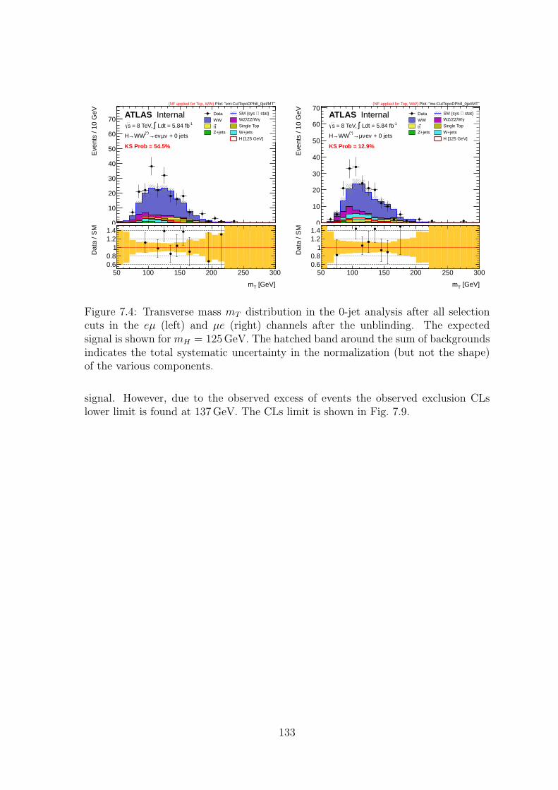
Eve
nts
/ 10
GeV
0
10
20
30
40
50
60
70 Data stat)⊕ SM (sys
WW γ WZ/ZZ/W
t t Single Top
Z+jets W+jets H [125 GeV]
ATLAS Internal
Plot: "em:CutTopoDPhill_0jet/MT"(NF applied for Top, WW)
-1 Ldt = 5.84 fb∫ = 8 TeV, s
+ 0 jetsνµνe→(*)WW→H
KS Prob = 54.5%
[GeV]Tm
50 100 150 200 250 300
Dat
a / S
M
0.60.8
11.21.4
Eve
nts
/ 10
GeV
0
10
20
30
40
50
60
70 Data stat)⊕ SM (sys
WW γ WZ/ZZ/W
t t Single Top
Z+jets W+jets H [125 GeV]
ATLAS Internal
Plot: "me:CutTopoDPhill_0jet/MT"(NF applied for Top, WW)
-1 Ldt = 5.84 fb∫ = 8 TeV, s
+ 0 jetsνeνµ→(*)WW→H
KS Prob = 12.9%
[GeV]Tm
50 100 150 200 250 300
Dat
a / S
M
0.60.8
11.21.4
Figure 7.4: Transverse mass mT distribution in the 0-jet analysis after all selectioncuts in the eµ (left) and µe (right) channels after the unblinding. The expectedsignal is shown for mH = 125 GeV. The hatched band around the sum of backgroundsindicates the total systematic uncertainty in the normalization (but not the shape)of the various components.
signal. However, due to the observed excess of events the observed exclusion CLslower limit is found at 137 GeV. The CLs limit is shown in Fig. 7.9.
133

[GeV]Hm110 120 130 140 150 160 170 180 190
0Lo
cal p
-710
-610
-510
-410
-310
-210
-1101
10
210
310
410
510Obs. Exp.
-1Ldt = 5.8 fb∫ = 8 TeV: s
ATLAS Preliminary
σ0σ1σ2
σ3
σ4
σ5
νeνµ/νµνe→(*)WW→H
[GeV]Hm115 120 125 130 135 140 145 150
)µS
igna
l str
engt
h (
0
2
4
6
8 Best fit
) < 1 µ(λ-2 ln -1Ldt = 5.8 fb∫ = 8 TeV: s
ATLAS Preliminary νeνµ/νµνe→(*)WW→H
Figure 7.5: 2012 results, using 5.8 fb−1 of 8 TeV data. Left: observed (solid line)probability for the background-only scenario as a function of mH . The dashed lineshows the corresponding expectation for the signal + background hypothesis at thegiven value of mH . Right: fitted signal strength parameter (µ) as a function of mH
for the low mass range.
[GeV]Tm
60 80 100 120 140 160 180 200 220 240
Eve
nts
/ 10
GeV
-20
0
20
40
60
80
100 Bkg. subtracted Data
H [125 GeV]
ATLAS Preliminary-1 Ldt = 4.7 fb∫ = 7 TeV, s
-1 Ldt = 5.8 fb∫ = 8 TeV, s
+ 0/1 jetsνlνl→(*)
WW→H
Figure 7.6: Distribution of mT in data with the estimated background subtracted,overlaid with the predicted signal for mH = 125GeV. The distributions are summedfor the 0- and 1-jet analyses and the 7 TeV and 8 TeV data. The statistical errors ofboth the data and the subtracted background are reflected in the data points. Thesystematic uncertainty on the background estimate is not included.
134
[GeV]Hm110 120 130 140 150 160 170 180 190
0Lo
cal p
-710
-610
-510
-410
-310
-210
-110
1
10
210
310Obs. Exp. -1Ldt = 5.8 fb∫ = 8 TeV: s
-1Ldt = 4.7 fb∫ = 7 TeV: s
ATLAS Preliminary
σ0σ1σ2
σ3
σ4
σ5
νlνl→(*)WW→H
[GeV]Hm115 120 125 130 135 140 145 150
)µS
igna
l str
engt
h (
0
1
2
3
4
5
6 Best fit ) < 1 µ(λ-2 ln = 125 GeV
HExp. m
) < 1 µ(λ-2 ln
-1Ldt = 5.8 fb∫ = 8 TeV: s
-1Ldt = 4.7 fb∫ = 7 TeV: s
ATLAS Preliminary νlνl→(*)WW→H
Figure 7.7: Combined 7 TeV and 8 TeV results. Left: observed (solid line) probabilityfor the background-only scenario as a function of mH . The dashed line shows thecorresponding expectation for the signal + background hypothesis at the given valueof mH . Right: fitted signal strength parameter (µ) as a function of mH for thelow mass range (solid black line with cyan band). The expected result for a signalhypothesis of mH = 125 GeV (red line) is included for comparison.
[GeV]Hm
115 120 125 130 135 140 145 150
)µS
igna
l str
engt
h (
0
1
2
3
4
5
6
0
2
4
6
8
10
12
) = 2.3H
,mµ(λ-2 ln
) = 6.0H
,mµ(λ-2 ln
(2011+2012)νlνl→(*)WW→H
(2011+2012)γγ→H
llll (2011+2012)→(*)ZZ→H
ATLAS Preliminary νlνl→(*)WW→H
-1Ldt = 4.7 fb∫ = 7 TeV: s-1Ldt = 5.8 fb∫ = 8 TeV: s
)H
,mµ(λ-ln
Figure 7.8: Approximate 68% and 95% two-dimensional likelihood (λ(µ,mH)) con-tours in the best-fit signal strength µ and mH for the WW (∗) → lνlν, ZZ(∗) → 4ℓ,and γγ analyses using the 2011 and 2012 data [123]. The yellow shading shows the− lnλ(µ,mH) values for H → WW (∗) → lνlν.
135
[GeV]Hm110 120 130 140 150 160 170 180 190
0Lo
cal p
-710
-610
-510
-410
-310
-210
-1101
10
210
310
410Obs.
= 125 GeVH
Exp. m
σ1 ±σ2 ±
-1Ldt = 5.8 fb∫ = 8 TeV: s
-1Ldt = 4.7 fb∫ = 7 TeV: s
ATLAS Preliminary
σ0σ1σ2
σ3
σ4
σ5
νlνl→(*)WW→H
[GeV]Hm115 120 125 130 135 140 145 150
SM
σ/σ95
% C
L Li
mit
on
-110
1
10
210Obs. Exp.
σ1 ±σ2 ±
-1Ldt = 5.8 fb∫ = 8 TeV: s
-1Ldt = 4.7 fb∫ = 7 TeV: s
ATLAS Preliminary νlνl→(*)WW→H
Figure 7.9: Left: Observed (solid line) probability for the background-only scenario,p0, as a function of mH , for the combined 7 TeV and 8 TeV data. The dashed lineshows the corresponding expectation for the mH = 125 GeV hypothesis. Right: Ob-served (solid) and expected (dashed) 95% CL upper limits on the cross section, nor-malized to the SM Higgs boson production cross section and as a function of mH ,over the full mass range considered in the 7 and 8 TeV combined data. Due to theexcess of events observed in the low mass signal region, the corresponding mass pointscannot be excluded as expected. The results at neighbouring mass points are highlycorrelated due to the limited mass resolution in this final state. The green and yel-low regions indicate the ±1σ and ±2σ uncertainty bands on the expected p0/limit,respectively.
136

137
Chapter 8
Drift Time Measurement in theATLAS Liquid Argon BarrelElectromagnetic Calorimeter
8.1 Introduction
In two recent ATLAS notes [128, 125], the measurement of the drift time of ionizationsignals in the liquid argon gap in the barrel part of the EM calorimeter and the gapuniformity was performed by using cosmic muon events and splash events in 2008and 2009, respectively. Similarly, in the summer of 2010 and March 2011, collisionevents were taken to be studied. The ionization pulses are sampled every 25 ns in 32samples for the study, while normally in collision events only 5 samples around thepeak of pulses are taken to measure the energy of each cell in the EM calorimeter.As described in [128, 125, 136], the drift time and the gap width are obtained fromfitting a predicted ionization pulse shape onto data collected with 32 samples. Bymeasuring the drift and gap width, one can access the intrinsic calorimeter uniformitywhich is directly related to the energy resolution constant term. The ionizationpulse shape can be predicted with the Response Transformation Method (RTM) [127]which is available from the entire EM (EMB and EMEC) and is used for the energyreconstruction in ATLAS. An alternative prediction based on the “First Principle”Method (FPM) [128] was developed for the EMB and is used in here with the resultsreported also in [137]. As shown in [136], both predictions give compatible results.
The barrel part of the EM calorimeter covers the pseudorapidity region |η| < 1.475whereas the two end cap parts cover the region 1.375 < |η| < 3.2. The EM liquidargon calorimeter is a highly granular sampling detector with accordion-shaped elec-trodes and lead absorbers and is fully symmetrical in the transverse plane. Granu-larities differ from layers in the barrel part of the liquid argon calorimeter [58] (seeTab. 8.1).
The drift time and the gap uniformity are two intrinsic parameters of the calorime-ter, their numerical values may be influenced by different methods and data samples,due to the particular structure of the detector and the different direction, multiplicity
138
Sampling layer Granularity η Granularity φ Coverage ηPS 0.025 0.1 |η| < 1.52Layer 1 0.003 0.1 |η| < 1.475Layer 2 0.025 0.025 |η| < 1.475Layer 3 0.05 0.025 |η| < 1.475
Table 8.1: Granularities and η coverage of the 4 layers in the barrel EM calorimeterwith PS standing for presampler.
of incoming particles. The cosmic muons preferentially travel through the detectorvertically and have in general a small multiplicity per triggered event. In the beamsplash event the horizontal incoming particles, which have a very large multiplicity,trigger essentially all cells at the same time. As a result, previous studies of thebeam splash data [125] showed evidence of a long range crosstalk effect between lay-ers, which resulted in discrepancies between cosmic muons and beam splash eventsin layer 3. However, in collision events, incoming particles originating from collisionvertices show different phenomena as well, which will be described in Section 8.4.This chapter is organized as follows: Section 8.2 gives the detail of data samples andthe fit method. Section 8.3 shows the results of fits to individual summed pulses. InSection 8.4 a crosstalk correction between neighbour cells in pseudorapidity directionin layer 1 is introduced. The drift time and gap uniformity results are shown in Sec-tion 8.5. In Section 8.6, an estimate of the sagging effect in the barrel part of thecalorimeter based on observed φ asymmetries is discussed.
8.2 Data Samples and Theoretical Model
The data were taken using L1Calo trigger in runs 160269 and 177960 in 2010 and2011, respectively. In the barrel parts, 2 387 415 pulses in 979 364 events in 2010 dataand 9 498 501 pulse in 700 224 events in 2011 high luminosity data were retrieved fromthe corresponding Event Summary Data (ESD) files with 1 GeV energy threshold onthe pulses. Meanwhile, to study the crosstalk effect between neighbour cells in layer1, a small sample of 50 236 events, corresponding to 408 931 pulses in 2010 data, wasreconstructed with a lower energy threshold of 200 MeV.
For the analysis, pulses are selected using cuts on the maximum amplitude (Smax)and shapes of the pulses, as described in note [128]. Table 8.2 shows the number ofpulses selected from the cosmic muons, beam splash and 2010, 2011 collision data,respectively. The 2010 collision data, which are used for fits to both individual andsummed pulses, have comparable statistics as the cosmic muon data in layer 2 andmore statistics in the presampler and layer 1. The 2011 collision data, which are11 times larger than the 2010 data, cover essentially all barrel calorimeter region (inparticular that in the back layer) and are used only for fits to summed pulses. InTable 8.2 a strong layer dependence is also shown. Layer 2 in collision data has morestatistics because more energy is deposited there and layer 1 gets fewer pulses due
139
Sampling layer / No. pulses collision 2011 collision 2010 splash cosmicPS 2.4 m 183 k 605.8 k 20.5 k
Layer 1 1.6 m 215 k 104.0 k 42.6 kLayer 2 5.4 m 760 k 2 233.9 k 330.3 kLayer 3 162 k 18.6 k 558.1 k 78.9 kTotal 9.5 m 1.2 m 3 501.8 k 472.3 k
Table 8.2: Number of selected pulses from 2010 and 2011 collision events in com-parison with the corresponding numbers from cosmic muon data and beam splashdata.
to the small cells and the energy threshold on Smax. Layer 3 is not well coveredin collision data because it is hard for electrons and photons to go through all thelayers. A comparison among the three data samples in Smax distribution is shownin Fig. 8.1 in different layers. The distribution of the maximum amplitude of thecollision events looks similar to the one of the cosmic muons because in these twocases the trajectory of incoming particles in the barrel is similar. The two thresholds(100 ADC and 160 ADC counts for |η| > 0.8 and |η| ≤ 0.8, respectively) on Smax inlayer 2 come from two different gains of the same energy threshold in different regions.The small sample which includes the cells in layer 1 with a lower energy threshold at200 MeV is not shown in Fig. 8.1.
A typical measured ionization signal shape is shown in Fig. 8.2 with the prediction.The signal pulse is recorded in 32 samples and the prediction, which is computed byFPM [128], is shown in 800 bins. A χ2 fit is performed by minimizing the followingχ2 function
χ2 =1
32 −Np
32∑
i=1
(
Si − SFPMi
σ
)2
, (8.1)
where Np is the number of free parameters fitted, Si(SFPMi ) are measured (predicted)
signal amplitude in bin i and σ is the noise term, which is taken as the RMS valueof the measured energy in pedestal runs and is about 8 ADC counts for the PS andlayer 1, 5 ADC counts for layer 2 (|η| ≤ 0.8) and layer 3 and 3.5 ADC counts for layer2 (|η| > 0.8).
In the FPM method, the predicted pulse is obtained by convolution in frequencydomain of a triangle like current signal with a transfer function of the electronic chaintaking into account of path lengths, impendences, skin effect parameters of cables,feedthroughs, the shaper and preamplifier transfer function. Some model parametersare extracted from generated electronic calibration pulses [128].
In the fit four free parameters are determined. They are
• the drift time (Tdrift) which is directly linked to the length of the undershoot ofthe pulse shape,
• the shift parameter (|δgap|) which affects the rise at the end of the pulse shapeand quantifies any asymmetry in size between the two gaps with respect to the
140
[ADC]maxS
0 1000 2000 3000
Ent
ry [a
.u.]
0
0.005
0.01
0.015
0.02
0.025 Collision0Entries 122414
Splash0Entries 605819
Cosmics0Entries 20546
PS
[ADC]maxS
0 1000 2000 3000
Ent
ry [a
.u.]
0
0.005
0.01
0.015
0.02
0.025
0.03
0.035 Collision1Entries 194429
Splash1Entries 104036
Cosmics1Entries 42563
Layer 1
[ADC]maxS
0 1000 2000 3000
Ent
ry [a
.u.]
0
0.002
0.004
0.006
0.008
0.01
0.012
0.014
0.016
0.018Collision2Entries 501153
Splash2Entries 2233929
Cosmics2Entries 330348
Layer 2
[ADC]maxS
0 1000 2000 3000
Ent
ry [a
.u.]
0
0.005
0.01
0.015
0.02
0.025
Collision3Entries 13436
Splash3Entries 558063
Cosmics3Entries 78881
Layer 3
Figure 8.1: Maximum amplitude Smax of the 2010 collision events (red) and beamsplash events (blue) and cosmic muon events (black) for four EM barrel samplinglayers. The histograms are normalized to unity. Note in layer 2 the two peaks at lowSmax correspond to two different gains for a same energy threshold.
nominal one (2.09 mm for layer 2 in the barrel),
• the maximum amplitude in terms of the number of ADC counts (Smax) whichmeasures the peak height of the pulse, and
• the timing (t0) which corresponds to the starting position of the pulse.
It should be pointed out that this is a cell based parameter determination. Eachelectronic cell is built out of several gaps connected in parallel: for layers 2 and 3,there are 4 double-gaps (one gap on each side of an electrode) in parallel in the barreland there are four times more gaps per cell in layer 1. The fitted parameters representthus an average of the local gaps, both in depth along the cell, and in between thegaps forming a cell.
141
t [ns]
0 100 200 300 400 500 600 700 800
S [A
DC
cou
nts]
-100
0
100
200
300ATLAS
2010 collision data
Figure 8.2: A typical pulse shape measured in ATLAS 2010 collision data (red his-togram) is shown with the corresponding fit results (blue dots) based on the FPMprediction.
8.3 Extracted Drift Time from Individual Pulses
and Summed Pulses
As it was done in the analysis of beam splash and cosmic muon events [125], fits areperformed pulse by pulse in 2010 collision data, which are called individual fits. Thefitted pulses are required to satisfy the following conditions. Only pulses recorded innominal voltage (2000 V) are considered (except for cells in the presampler of the 2011collision data, where the nominal voltage is reduced to 1600V), the voltage shouldbe symmetric in both sides of the gap and a series quality cuts are also applied onthe pulse shapes [128]. What is different from the previous study is that the 2010collision events have a large fraction of pulses with small amplitude. These pulsesare likely to fluctuate in pulse shape so that they may be rejected by the qualityrequirement. The fluctuation in the tail of the pulse shapes also results in a largeuncertainty in the fitted parameters. The fitted drift time (Tdrift) and gap asymmetry(|δgap|) are shown in Figs. 8.3 and 8.4 respectively, in comparison with similar resultsbased on the cosmic muon and beam splash events. In the figure a χ2
n cut is applied,where χ2
n is a normalized χ2 and it differs from that of Eq. 8.1 in that σ2 is replacedby σ2 + (kSmax)
2, to take into account the uncertainty of the predicted amplitude.The layer dependent k-factors are chosen to have the values of 0.9%, 1.1%, 0.8% and0.75% [128] for the PS, layers 1, 2 and 3, respectively, such that the χ2
n is in averageindependent of Smax. Figures 8.3 and 8.4 show large RMS values in both the drifttime and the gap asymmetry, due to the fluctuation in the individual pulses.
To reduce the fluctuation, fits to summed pulses (summed fits) are performed.The summed pulses are the average of individual pulses. That means pulses in asame cell are added up event by event directly when they have the same timing. The32 samples are converted to 800 samples to perform the fit. Figure 8.5 shows the
142
[ns]driftT
300 400 500 600 700 800
Ent
ry [a
.u.]
0
0.01
0.02
0.03
0.04
0.05
0.06
0.07
Collision0Entries 180800Mean 424RMS 26.8
Splash0Entries 579656Mean 428.6RMS 12.54
Cosmics0Entries 19942Mean 430.2RMS 17.66
PS
[ns]driftT
300 400 500 600 700 800
Ent
ry [a
.u.]
0
0.01
0.02
0.03
0.04
0.05
0.06
0.07
Collision1Entries 215271Mean 467.7RMS 20
Splash1Entries 96698Mean 453.8RMS 23.59
Cosmics1Entries 40430Mean 459.7RMS 33.58
Layer 1
[ns]driftT
300 400 500 600 700 800
Ent
ry [a
.u.]
0
0.01
0.02
0.03
0.04
0.05
0.06
0.07
Collision2Entries 757718Mean 456.4RMS 17.93
Splash2Entries 1826076Mean 450.4RMS 14.65
Cosmics2Entries 317297Mean 457.4RMS 21.86
Layer 2
[ns]driftT
300 400 500 600 700 800
Ent
ry [a
.u.]
0
0.01
0.02
0.03
0.04
0.05
0.06
0.07
Collision3Entries 18569Mean 459.7RMS 17.08
Splash3Entries 429077Mean 446.7RMS 24.77
Cosmics3Entries 76749Mean 463RMS 25.38
Layer 3
Figure 8.3: Extracted drift time (Tdrift) from fits to individual pulses in the 2010collision events, 2009 splash events and 2008 cosmic muon events, for four EM barrelcalorimeter layers.
143
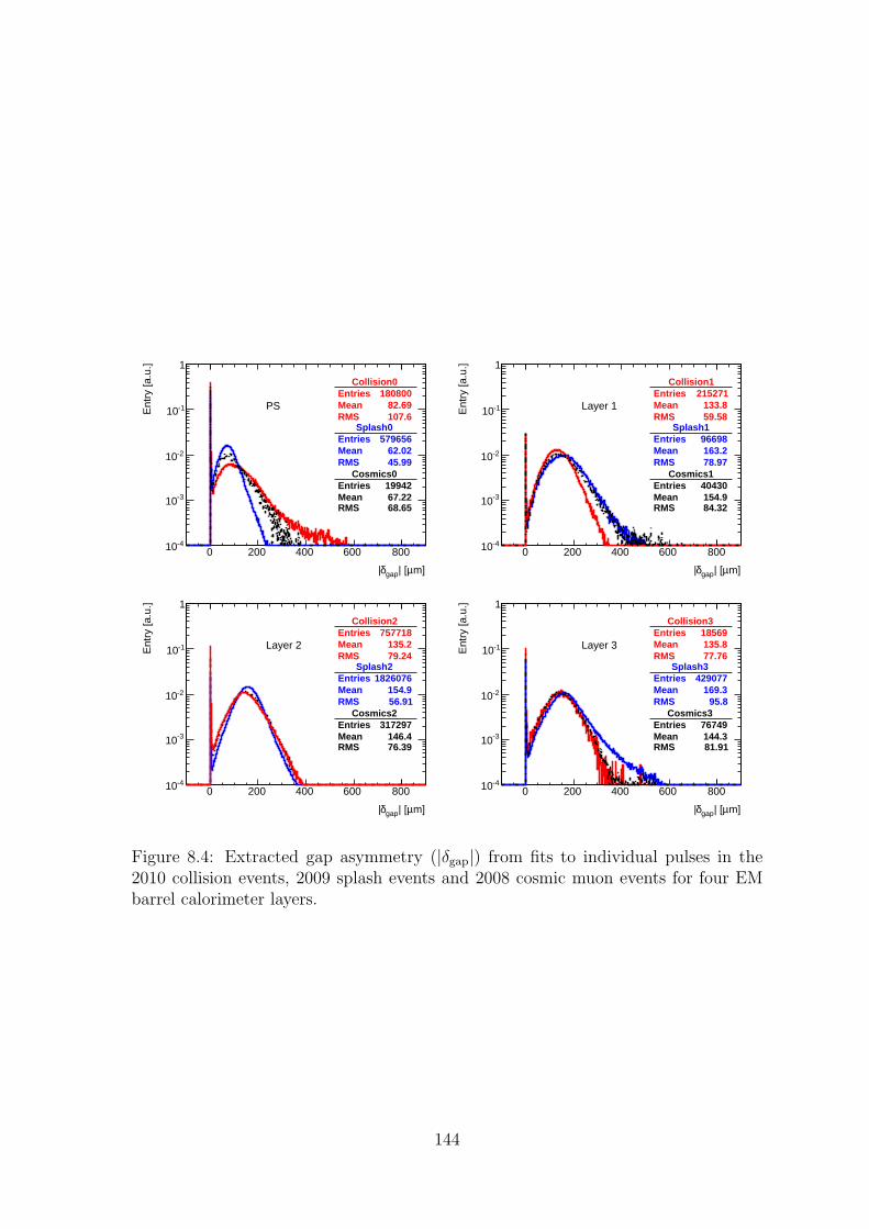
m]µ| [gapδ|
0 200 400 600 800
Ent
ry [a
.u.]
-410
-310
-210
-110
1
Collision0Entries 180800Mean 82.69RMS 107.6
Splash0Entries 579656Mean 62.02RMS 45.99
Cosmics0Entries 19942Mean 67.22RMS 68.65
PS
m]µ| [gapδ|
0 200 400 600 800
Ent
ry [a
.u.]
-410
-310
-210
-110
1
Collision1Entries 215271Mean 133.8RMS 59.58
Splash1Entries 96698Mean 163.2RMS 78.97
Cosmics1Entries 40430Mean 154.9RMS 84.32
Layer 1
m]µ| [gapδ|
0 200 400 600 800
Ent
ry [a
.u.]
-410
-310
-210
-110
1
Collision2Entries 757718Mean 135.2RMS 79.24
Splash2Entries 1826076Mean 154.9RMS 56.91
Cosmics2Entries 317297Mean 146.4RMS 76.39
Layer 2
m]µ| [gapδ|
0 200 400 600 800
Ent
ry [a
.u.]
-410
-310
-210
-110
1
Collision3Entries 18569Mean 135.8RMS 77.76
Splash3Entries 429077Mean 169.3RMS 95.8
Cosmics3Entries 76749Mean 144.3RMS 81.91
Layer 3
Figure 8.4: Extracted gap asymmetry (|δgap|) from fits to individual pulses in the2010 collision events, 2009 splash events and 2008 cosmic muon events for four EMbarrel calorimeter layers.
144
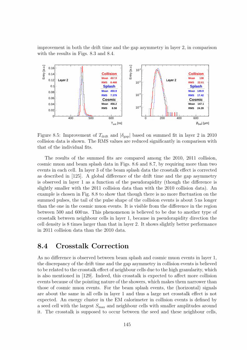
improvement in both the drift time and the gap asymmetry in layer 2, in comparisonwith the results in Figs. 8.3 and 8.4.
[ns]driftT
400 500 600
Ent
ry [a
.u.]
0
0.02
0.04
0.06
0.08
0.1
0.12
0.14
0.16
Layer 2
CollisionMean 457.9
RMS 8.468Layer 2
SplashMean 450.9
RMS 7.379
CosmicMean 456.2
RMS 8.58
m]µ| [gapδ|
0 200 400 600
Ent
ry [a
.u.]
-410
-310
-210
-110
Layer 2
CollisionMean 138
RMS 22.61Layer 2
SplashMean 149.9
RMS 17.42
CosmicMean 147.1
RMS 24.39
Figure 8.5: Improvement of Tdrift and |δgap| based on summed fit in layer 2 in 2010collision data is shown. The RMS values are reduced significantly in comparison withthat of the individual fits.
The results of the summed fits are compared among the 2010, 2011 collision,cosmic muon and beam splash data in Figs. 8.6 and 8.7, by requiring more than twoevents in each cell. In layer 3 of the beam splash data the crosstalk effect is correctedas described in [125]. A global difference of the drift time and the gap asymmetryis observed in layer 1 as a function of the pseudorapidity (though the difference isslightly smaller with the 2011 collision data than with the 2010 collision data). Anexample is chosen in Fig. 8.8 to show that though there is no more fluctuation on thesummed pulses, the tail of the pulse shape of the collision events is about 5 ns longerthan the one in the cosmic muon events. It is visible from the difference in the regionbetween 500 and 600 ns. This phenomenon is believed to be due to another type ofcrosstalk between neighbour cells in layer 1, because in pseudorapidity direction thecell density is 8 times larger than that in layer 2. It shows slightly better performancein 2011 collision data than the 2010 data.
8.4 Crosstalk Correction
As no difference is observed between beam splash and cosmic muon events in layer 1,the discrepancy of the drift time and the gap asymmetry in collision events is believedto be related to the crosstalk effect of neighbour cells due to the high granularity, whichis also mentioned in [129]. Indeed, this crosstalk is expected to affect more collisionevents because of the pointing nature of the showers, which makes them narrower thanthose of cosmic muon events. For the beam splash events, the (horizontal) signalsare about the same in all cells in layer 1 and thus a large net crosstalk effect is notexpected. An energy cluster in the EM calorimeter in collision events is defined bya seed cell with the largest Smax and neighbour cells with smaller amplitudes aroundit. The crosstalk is supposed to occur between the seed and these neighbour cells,
145
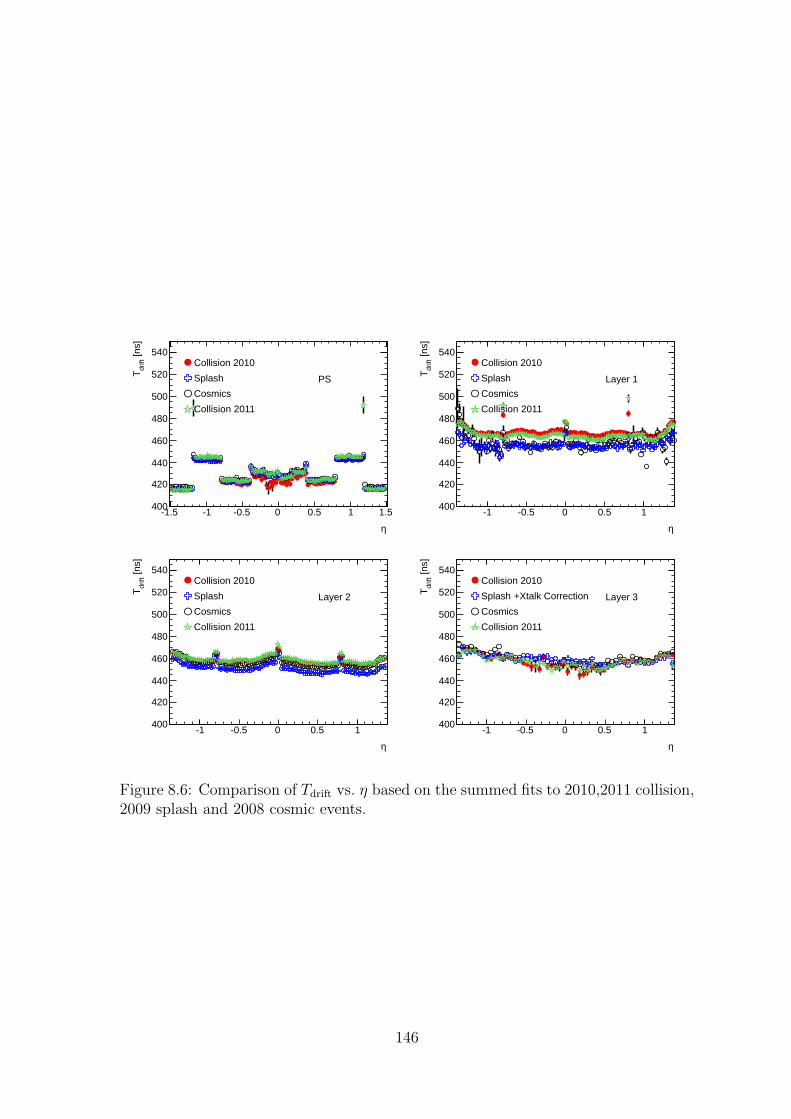
η
-1.5 -1 -0.5 0 0.5 1 1.5
[ns]
drift
T
400
420
440
460
480
500
520
540Collision 2010
Splash
Cosmics
Collision 2011
PS
η
-1 -0.5 0 0.5 1
[ns]
drift
T
400
420
440
460
480
500
520
540Collision 2010
Splash
Cosmics
Collision 2011
Layer 1
η
-1 -0.5 0 0.5 1
[ns]
drift
T
400
420
440
460
480
500
520
540Collision 2010
Splash
Cosmics
Collision 2011
Layer 2
η
-1 -0.5 0 0.5 1
[ns]
drift
T
400
420
440
460
480
500
520
540Collision 2010
Splash
Cosmics
Collision 2011
Layer 3+Xtalk Correction
Figure 8.6: Comparison of Tdrift vs. η based on the summed fits to 2010,2011 collision,2009 splash and 2008 cosmic events.
146
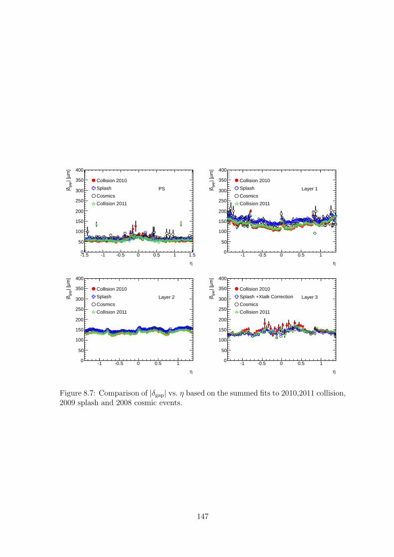
η
-1.5 -1 -0.5 0 0.5 1 1.5
m]
µ| [
gap
δ|
0
50
100
150
200
250
300
350
400
Collision 2010
Splash
Cosmics
Collision 2011
PS
η
-1 -0.5 0 0.5 1
m]
µ| [
gap
δ|
0
50
100
150
200
250
300
350
400
Collision 2010
Splash
Cosmics
Collision 2011
Layer 1
η
-1 -0.5 0 0.5 1
m]
µ| [
gap
δ|
0
50
100
150
200
250
300
350
400
Collision 2010
Splash
Cosmics
Collision 2011
Layer 2
η
-1 -0.5 0 0.5 1
m]
µ| [
gap
δ|
0
50
100
150
200
250
300
350
400
Collision 2010
Splash
Cosmics
Collision 2011
Layer 3+Xtalk Correction
Figure 8.7: Comparison of |δgap| vs. η based on the summed fits to 2010,2011 collision,2009 splash and 2008 cosmic events.
147
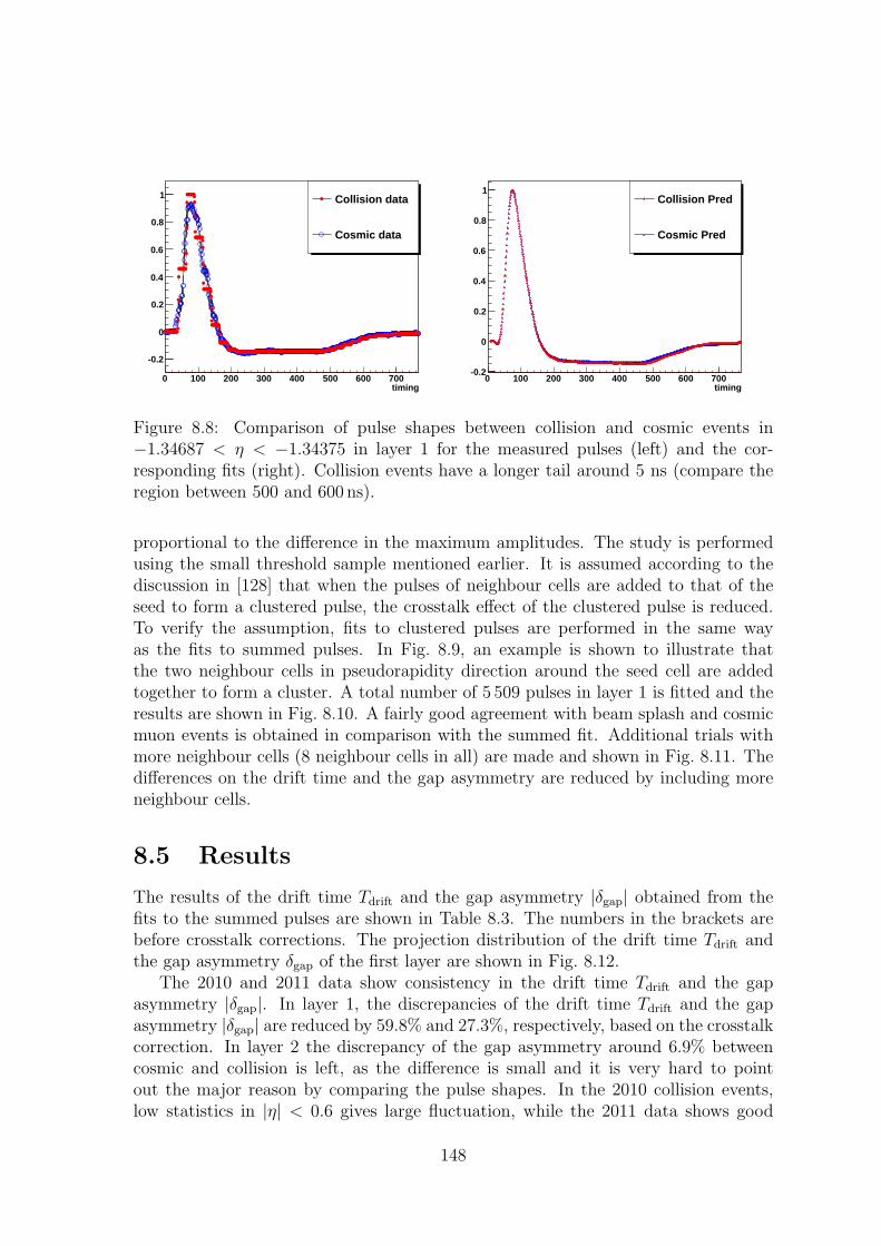
timing0 100 200 300 400 500 600 700
-0.2
0
0.2
0.4
0.6
0.8
1 Collision data
Cosmic data
timing0 100 200 300 400 500 600 700
-0.2
0
0.2
0.4
0.6
0.8
1Collision Pred
Cosmic Pred
Figure 8.8: Comparison of pulse shapes between collision and cosmic events in−1.34687 < η < −1.34375 in layer 1 for the measured pulses (left) and the cor-responding fits (right). Collision events have a longer tail around 5 ns (compare theregion between 500 and 600 ns).
proportional to the difference in the maximum amplitudes. The study is performedusing the small threshold sample mentioned earlier. It is assumed according to thediscussion in [128] that when the pulses of neighbour cells are added to that of theseed to form a clustered pulse, the crosstalk effect of the clustered pulse is reduced.To verify the assumption, fits to clustered pulses are performed in the same wayas the fits to summed pulses. In Fig. 8.9, an example is shown to illustrate thatthe two neighbour cells in pseudorapidity direction around the seed cell are addedtogether to form a cluster. A total number of 5 509 pulses in layer 1 is fitted and theresults are shown in Fig. 8.10. A fairly good agreement with beam splash and cosmicmuon events is obtained in comparison with the summed fit. Additional trials withmore neighbour cells (8 neighbour cells in all) are made and shown in Fig. 8.11. Thedifferences on the drift time and the gap asymmetry are reduced by including moreneighbour cells.
8.5 Results
The results of the drift time Tdrift and the gap asymmetry |δgap| obtained from thefits to the summed pulses are shown in Table 8.3. The numbers in the brackets arebefore crosstalk corrections. The projection distribution of the drift time Tdrift andthe gap asymmetry δgap of the first layer are shown in Fig. 8.12.
The 2010 and 2011 data show consistency in the drift time Tdrift and the gapasymmetry |δgap|. In layer 1, the discrepancies of the drift time Tdrift and the gapasymmetry |δgap| are reduced by 59.8% and 27.3%, respectively, based on the crosstalkcorrection. In layer 2 the discrepancy of the gap asymmetry around 6.9% betweencosmic and collision is left, as the difference is small and it is very hard to pointout the major reason by comparing the pulse shapes. In the 2010 collision events,low statistics in |η| < 0.6 gives large fluctuation, while the 2011 data shows good
148
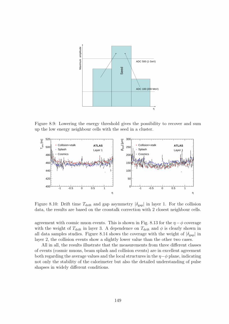
�
����
����AA�BC�D�EF
����CAA�B�AA���EF
�����
��
����
�������
Figure 8.9: Lowering the energy threshold gives the possibility to recover and sumup the low energy neighbour cells with the seed in a cluster.
η-1 -0.5 0 0.5 1
[ns]
drfit
T
400
420
440
460
480
500
520
ATLAS
Layer 1
Collision+xtalk
Splash
Cosmics
η-1 -0.5 0 0.5 1
m]
µ| [
gap
δ|
0
50
100
150
200
250
300
ATLAS
Layer 1
Collision+xtalk
Splash
Cosmics
Figure 8.10: Drift time Tdrift and gap asymmetry |δgap| in layer 1. For the collisiondata, the results are based on the crosstalk correction with 2 closest neighbour cells.
agreement with cosmic muon events. This is shown in Fig. 8.13 for the η−φ coveragewith the weight of Tdrift in layer 3. A dependence on Tdrift and φ is clearly shown inall data samples studies. Figure 8.14 shows the coverage with the weight of |δgap| inlayer 2, the collision events show a slightly lower value than the other two cases.
All in all, the results illustrate that the measurements from three different classesof events (cosmic muons, beam splash and collision events) are in excellent agreementboth regarding the average values and the local structures in the η−φ plane, indicatingnot only the stability of the calorimeter but also the detailed understanding of pulseshapses in widely different conditions.
149
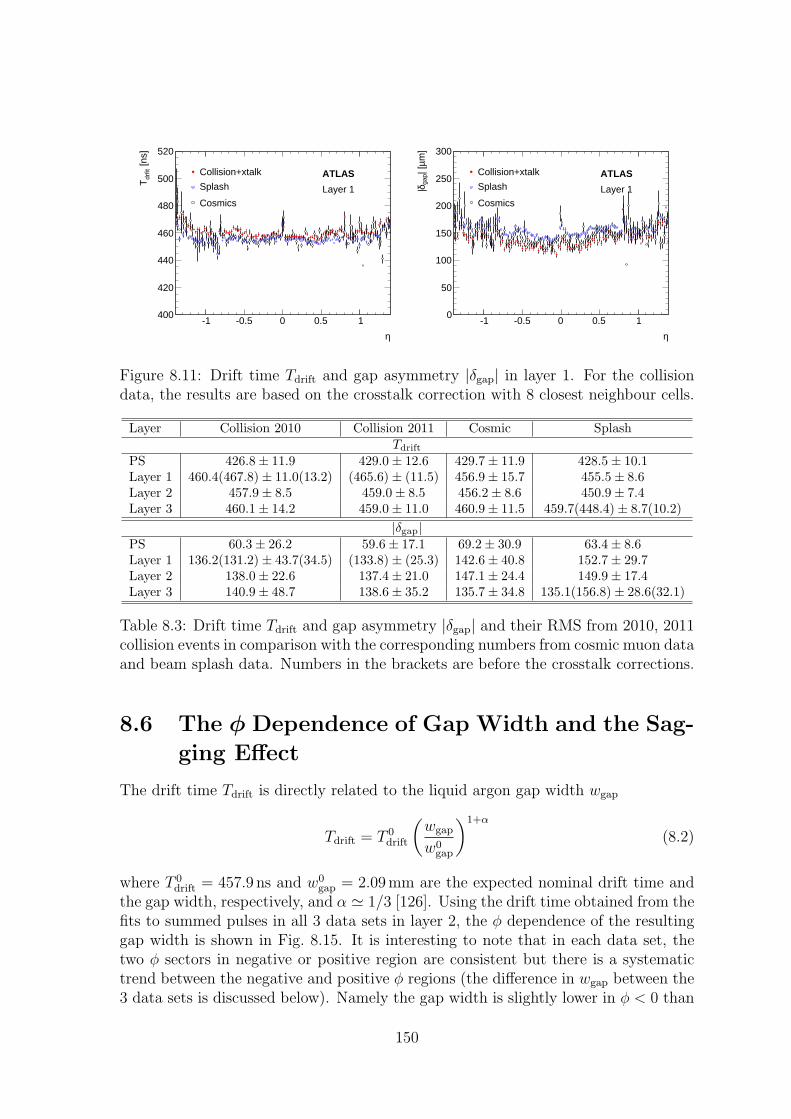
η-1 -0.5 0 0.5 1
[ns]
drfit
T
400
420
440
460
480
500
520
ATLAS
Layer 1
Collision+xtalk
Splash
Cosmics
η-1 -0.5 0 0.5 1
m]
µ| [
gap
δ|
0
50
100
150
200
250
300
ATLAS
Layer 1
Collision+xtalk
Splash
Cosmics
Figure 8.11: Drift time Tdrift and gap asymmetry |δgap| in layer 1. For the collisiondata, the results are based on the crosstalk correction with 8 closest neighbour cells.
Layer Collision 2010 Collision 2011 Cosmic SplashTdrift
PS 426.8 ± 11.9 429.0 ± 12.6 429.7 ± 11.9 428.5 ± 10.1Layer 1 460.4(467.8) ± 11.0(13.2) (465.6) ± (11.5) 456.9 ± 15.7 455.5 ± 8.6Layer 2 457.9 ± 8.5 459.0 ± 8.5 456.2 ± 8.6 450.9 ± 7.4Layer 3 460.1 ± 14.2 459.0 ± 11.0 460.9 ± 11.5 459.7(448.4) ± 8.7(10.2)
|δgap|PS 60.3 ± 26.2 59.6 ± 17.1 69.2 ± 30.9 63.4 ± 8.6Layer 1 136.2(131.2) ± 43.7(34.5) (133.8) ± (25.3) 142.6 ± 40.8 152.7 ± 29.7Layer 2 138.0 ± 22.6 137.4 ± 21.0 147.1 ± 24.4 149.9 ± 17.4Layer 3 140.9 ± 48.7 138.6 ± 35.2 135.7 ± 34.8 135.1(156.8) ± 28.6(32.1)
Table 8.3: Drift time Tdrift and gap asymmetry |δgap| and their RMS from 2010, 2011collision events in comparison with the corresponding numbers from cosmic muon dataand beam splash data. Numbers in the brackets are before the crosstalk corrections.
8.6 The φ Dependence of Gap Width and the Sag-
ging Effect
The drift time Tdrift is directly related to the liquid argon gap width wgap
Tdrift = T 0drift
(
wgap
w0gap
)1+α
(8.2)
where T 0drift = 457.9 ns and w0
gap = 2.09mm are the expected nominal drift time andthe gap width, respectively, and α ≃ 1/3 [126]. Using the drift time obtained from thefits to summed pulses in all 3 data sets in layer 2, the φ dependence of the resultinggap width is shown in Fig. 8.15. It is interesting to note that in each data set, thetwo φ sectors in negative or positive region are consistent but there is a systematictrend between the negative and positive φ regions (the difference in wgap between the3 data sets is discussed below). Namely the gap width is slightly lower in φ < 0 than
150
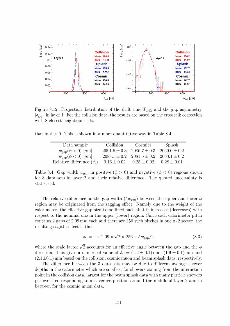
[ns]driftT
400 500 600
Ent
ry [a
.u.]
0
0.02
0.04
0.06
0.08
0.1
0.12
0.14
Layer 1
CollisionMean 460.4
RMS 11.01Layer 1
SplashMean 455.5
RMS 8.652
CosmicMean 456.8
RMS 14.99
m]µ| [gapδ|
0 200 400 600
Ent
ry [a
.u.]
-410
-310
-210
-110
Layer 1
CollisionMean 136.2
RMS 43.67Layer 1
SplashMean 152.7
RMS 29.81
CosmicMean 142.7
RMS 41.62
Figure 8.12: Projection distribution of the drift time Tdrift and the gap asymmetry|δgap| in layer 1. For the collision data, the results are based on the crosstalk correctionwith 8 closest neighbour cells.
that in φ > 0. This is shown in a more quantitative way in Table 8.4.
Data sample Collision Cosmics Splashwgap(φ > 0) [µm] 2091.5 ± 0.3 2086.7 ± 0.3 2069.0 ± 0.2wgap(φ < 0) [µm] 2088.1 ± 0.2 2081.5 ± 0.2 2063.1 ± 0.2
Relative difference (%) 0.16 ± 0.02 0.25 ± 0.02 0.28 ± 0.01
Table 8.4: Gap width wgap in positive (φ > 0) and negative (φ < 0) regions shownfor 3 data sets in layer 2 and their relative difference. The quoted uncertainty isstatistical.
The relative difference on the gap width (δwgap) between the upper and lower φregion may be originated from the sagging effect. Namely due to the weight of thecalorimeter, the effective gap size is modified such that it increases (decreases) withrespect to the nominal one in the upper (lower) region. Since each calorimeter pitchcontains 2 gaps of 2.09mm each and there are 256 such pitches in one π/2 sector, theresulting sagitta effect is thus
δc = 2 × 2.09 ×√
2 × 256 × δwgap/2 (8.3)
where the scale factor√
2 accounts for an effective angle between the gap and the φdirection. This gives a numerical value of δc = (1.2 ± 0.1) mm, (1.9 ± 0.1) mm and(2.1±0.1) mm based on the collision, cosmic muon and beam splash data, respectively.
The difference between the 3 data sets may be due to different average showerdepths in the calorimeter which are smallest for showers coming from the interactionpoint in the collision data, largest for the beam splash data with many particle showersper event corresponding to an average position around the middle of layer 2 and inbetween for the cosmic muon data.
151
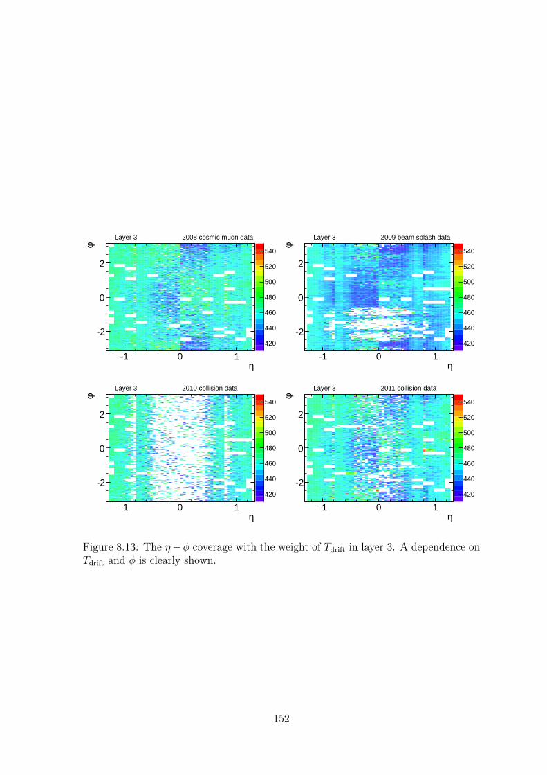
420
440
460
480
500
520
540
η-1 0 1
φ
-2
0
2
Layer 3 2008 cosmic muon data
420
440
460
480
500
520
540
η-1 0 1
φ
-2
0
2
Layer 3 2009 beam splash data
420
440
460
480
500
520
540
η-1 0 1
φ
-2
0
2
Layer 3 2010 collision data
420
440
460
480
500
520
540
η-1 0 1
φ
-2
0
2
Layer 3 2011 collision data
Figure 8.13: The η−φ coverage with the weight of Tdrift in layer 3. A dependence onTdrift and φ is clearly shown.
152
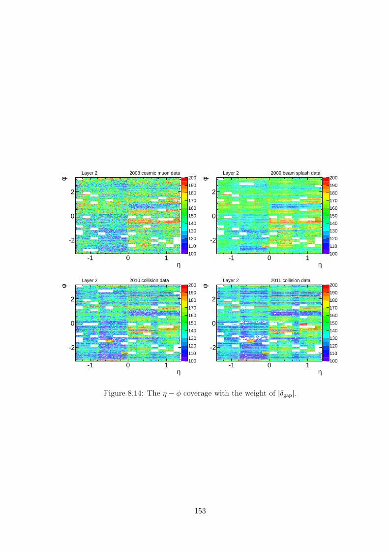
100
110
120
130
140
150
160
170
180
190
200
η-1 0 1
φ
-2
0
2
Layer 2 2008 cosmic muon data
100
110
120
130
140
150
160
170
180
190
200
η-1 0 1
φ
-2
0
2
Layer 2 2009 beam splash data
100
110
120
130
140
150
160
170
180
190
200
η-1 0 1
φ
-2
0
2
Layer 2 2010 collision data
100
110
120
130
140
150
160
170
180
190
200
η-1 0 1
φ
-2
0
2
Layer 2 2011 collision data
Figure 8.14: The η − φ coverage with the weight of |δgap|.
153
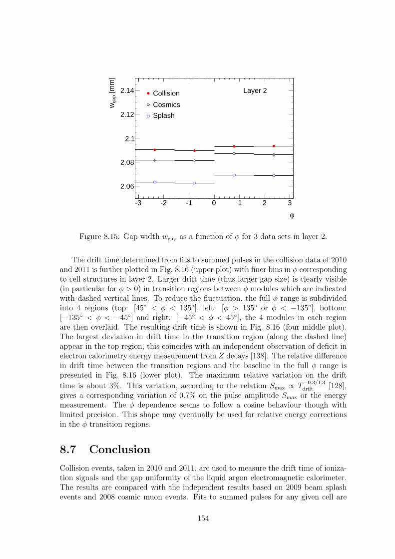
φ
-3 -2 -1 0 1 2 3
[mm
]ga
pw
2.06
2.08
2.1
2.12
2.14 Layer 2Collision
Cosmics
Splash
Figure 8.15: Gap width wgap as a function of φ for 3 data sets in layer 2.
The drift time determined from fits to summed pulses in the collision data of 2010and 2011 is further plotted in Fig. 8.16 (upper plot) with finer bins in φ correspondingto cell structures in layer 2. Larger drift time (thus larger gap size) is clearly visible(in particular for φ > 0) in transition regions between φ modules which are indicatedwith dashed vertical lines. To reduce the fluctuation, the full φ range is subdividedinto 4 regions (top: [45◦ < φ < 135◦], left: [φ > 135◦ or φ < −135◦], bottom:[−135◦ < φ < −45◦] and right: [−45◦ < φ < 45◦], the 4 modules in each regionare then overlaid. The resulting drift time is shown in Fig. 8.16 (four middle plot).The largest deviation in drift time in the transition region (along the dashed line)appear in the top region, this coincides with an independent observation of deficit inelectron calorimetry energy measurement from Z decays [138]. The relative differencein drift time between the transition regions and the baseline in the full φ range ispresented in Fig. 8.16 (lower plot). The maximum relative variation on the drift
time is about 3%. This variation, according to the relation Smax ∝ T−0.3/1.3drift [128],
gives a corresponding variation of 0.7% on the pulse amplitude Smax or the energymeasurement. The φ dependence seems to follow a cosine behaviour though withlimited precision. This shape may eventually be used for relative energy correctionsin the φ transition regions.
8.7 Conclusion
Collision events, taken in 2010 and 2011, are used to measure the drift time of ioniza-tion signals and the gap uniformity of the liquid argon electromagnetic calorimeter.The results are compared with the independent results based on 2009 beam splashevents and 2008 cosmic muon events. Fits to summed pulses for any given cell are
154
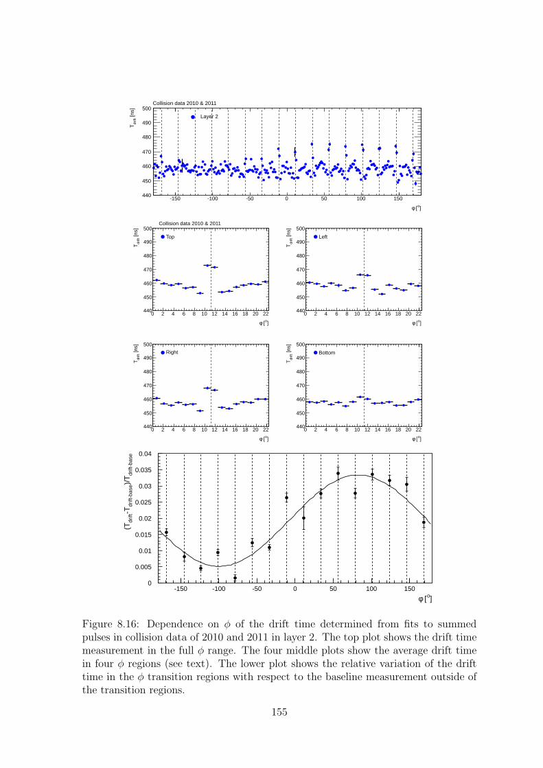
]o [φ
-150 -100 -50 0 50 100 150
[ns]
drift
T
440
450
460
470
480
490
500
Layer 2
Collision data 2010 & 2011
]o [φ
0 2 4 6 8 10 12 14 16 18 20 22
[ns]
drift
T
440
450
460
470
480
490
500
Top
Collision data 2010 & 2011
]o [φ
0 2 4 6 8 10 12 14 16 18 20 22
[ns]
drift
T
440
450
460
470
480
490
500
Left
]o [φ
0 2 4 6 8 10 12 14 16 18 20 22
[ns]
drift
T
440
450
460
470
480
490
500
Right
]o [φ
0 2 4 6 8 10 12 14 16 18 20 22
[ns]
drift
T
440
450
460
470
480
490
500
Bottom
0
0.005
0.01
0.015
0.02
0.025
0.03
0.035
0.04
-150 -100 -50 0 50 100 150
φ [o]
(Tdr
ift-T
drift
-bas
e)/T
drift
-bas
e
Figure 8.16: Dependence on φ of the drift time determined from fits to summedpulses in collision data of 2010 and 2011 in layer 2. The top plot shows the drift timemeasurement in the full φ range. The four middle plots show the average drift timein four φ regions (see text). The lower plot shows the relative variation of the drifttime in the φ transition regions with respect to the baseline measurement outside ofthe transition regions.
155

performed to reduce the fluctuation in the pulse shapes. The crosstalk effect in elec-trical signals between neighbour cells in layer 1 is studied. The crosstalk effect islargely canceled when adding all cells in a cluster. Overall for both the drift time andthe gap asymmetry an excellent agreement between data samples is observed, thougha small difference in the gap asymmetry in layer 2 between collision events and cosmicmuon events still remains, which cannot be easily corrected for without knowing thepulse shape of the crosstalk contribution. In the barrel part of the calorimeter, thesagging effect corresponding to numerical values of 1.2− 2.1 mm is observed from theasymmetry measured in cells between the positive and negative φ sectors.
156

157
Conclusion
A Higgs boson search in the H → WW (∗) → lνlν channel has been performed. Thesearch in the SM uses all available data taken by the ATLAS experiment at the LHC in2011 and 2012 at
√s = 7 TeV and 8 TeV, respectively. The corresponding integrated
luminosity values are 4.7 fb−1 in 2011 and 5.8 fb−1 in 2012. Due to the increasedsearch sensitivity for a Higgs boson in a four generation model with additional heavyquarks, the analysis in the WW (∗) channel based on the early data of 2011 was alsocombined with those in other channels to search for a fourth generation Higgs boson.In both cases, the WW (∗) channel has the dominant sensitivity for a large part of themass range 110 − 600 GeV covered by all combined channels.
The published analysis in the WW (∗) channel is cut based, exploiting a cleanfinal state signature with two isolated leptons and large missing transverse energyEmiss
T,rel. The transverse momenta of the leading and subleading leptons are required tobe greater than 25 GeV and 15 GeV, respectively. The larger transverse momentumvalue for the leading lepton guarantees a very efficient trigger of the event. The leptoncan be either an electron or a muon, resulting in thus three flavour combinations:ee, µµ and eµ. More stringent cut on the transverse missing energy in the sameflavour channels is imposed to suppress the larger Drell-Yan background contributionsthere. For this reason, the first result of the 2012 data analysis is limited to the eµchannel (including µe) which has the dominant sensitivity due mainly to its smallerbackground contamination. The analyses are further categorized in 0-, 1- and 2-jet channels to cope with different background contributions. The dominant topbackground events are rejected using the b-jet veto. Several topological cuts (e.g.∆φll, p
llT , mll) are further applied to suppress the remaining Drell-Yan and the SM
WW irreducible backgrounds.In the analysis, several data-driven background methods are used to extract the
expected background contamination in data. The W+jets events are extracted us-ing fake rate determined in the QCD jet enriched samples. The Z+jets events areestimated using the ABCD method, extrapolating from the Z mass window to thesignal region. The top background estimation in 0-jet bin is made using a data-drivenmethod that we have proposed, which derives both the top normalisation and the jetveto survival probability from data. The method is robust against the jet energyscale and resolution variations which would have been the dominant systematic un-certainties. The systematic uncertainties of the method have been thoroughly studiedincluding several closure tests. The method has been used in a number of ATLASanalyses including the SM WW cross section measurement and searches for super-
158
symmetric particles [132, 133]. For the Higgs search in the WW (∗) channel, it hasbeen the baseline method since the very beginning of the data analysis.
To cross check the ABCD method, we have proposed an alternative data-drivenmethod to estimate the Z+jets background contribution by correcting the Emiss
T dis-tribution in the Drell-Yan sample using larger statistics sample of W+jets events.The method exploits the fake Emiss
T shape in the W+jets sample after subtracting theneutrino transverse momentum. The method has been tested in two different setsof MC samples used for the 2011 data analysis. The method works independentlyof larger or smaller Emiss
T mismodelling. The results derived using this method areconsistent with that of the ABCD method and have the advantage in that the estima-tion is more precise and the normalisation factor is not affected by further topologicalcuts.
Based on the enhanced Higgs production cross section and modified decay branch-ing fractions that we evaluated for a fourth generation scenario, the search excludessuch a fourth generation Higgs boson essentially in the full mass range 120−600 GeVat 95%CL.
In 2011, the SM Higgs boson is excluded in the H → WW (∗) → lνlν channel from133 GeV to 261 GeV at 95%CL while the expected exclusion limits are 127−234 GeV.In 2012, a significant excess of events is observed over the expected background.Combining 2011 and 2012 data, the minimum observed p0 value, found at mH =125 GeV, is 3 × 10⁻³, corresponding to 2.8 standard deviations (3.1σ in 2012 alone).The expected p0 for a Higgs at the same mass is 0.01 or 2.3σ. The fitted signalstrength at mH = 125 GeV is µ = 1.4 ± 0.5.
Independent of the Higgs searches, an additional study is performed on the elec-tron drift time in the liquid Argon (LAr) calorimeter in the ATLAS detector usingdedicated data samples taken in 2008, 2009, 2010 and 2011 from cosmic rays, beamsplash and beam collision events. The first principle method is used to analyze overmore than 5 million single pulse shapes taken in each cell of the LAr calorimeterbarrel part. Fits both to individual pulses and to summed pulses over all events areperformed. The result shows no significant deviation on gap width in each cell inthe calorimeter and the sagging effect due to the gravity effect on the calorimeter isobserved.
Together with the other decay channels in particular the γγ and ZZ(∗) → 4lchannels, both ATLAS and CMS experiments have observed a SM-like Higgs bosonat mass around 125 GeV. Now the new focus is moved to measure the propertiesof the newly discovered particle to check whether it is indeed the SM Higgs boson.For this purpose, high statistical data sample is needed. The LHC is continuing the8 TeV running till the end of 2012, extending by two more months of data takingoriginally foreseen. More than 15 fb−1 additional integrated luminosity is expected.In parallel, the analysis is being further improved by using multivariate techniquesfor object and event selections and by enlarging the phase space of the signal regione.g. to lower transverse momentum of 10GeV for the subleading leptons. If the newparticle is confirmed to be the SM Higgs boson, the SM will be complete. However,the existence of the Higgs boson in turn introduces the problem of gauge hierarchy,namely the fact that in the presence of new physics the Higgs mass and the weak
159

scale itself are destabilized towards higher energy scale by quantum corrections. Itis generally believed that the SM of particle physics is only an effective theory of amore fundamental underlying theory. Therefore search for new physics at the LHCwill be the next major goal.
160
Bibliography
[1] M. Banner et al. (UA2 Collaboration), Phys. Lett. B. 122, 476 (1983).
[2] P. Bagnaia et al. (UA2 Collaboration), Phys. Lett. B. 129, 130 (1983).
[3] S. Abachi et al. (D0 Collaboration), Phys. Rev. Lett. 74, 2632 (1995).
[4] Donald H. Perkins, “Introduction to High Energy Physics”, Cambridge Uni-versity press 4th Edition.
[5] V.V. Ezhela, S.B. Lugovsky, O.V. Zenin, “Hadronic Part of the Muon g-2 Es-timated on the σ2003
tot (e+e− → hadrons) Evaluated Data Compilation”, arXiv:hep-ph/0312114. Jan 2004.
[6] L. O’Raifeartaigh, N. Straumann, “Early History of Gauge Theories andKaluza-Klein Theories, with a Glance at Recent Developments”, arXiv: hep-ph/9810524. Apr 1999.
[7] C. N. Yang, R. Mills, Phys. Rev. 96, 191 (1954).
[8] S. Glashow, Nucl. Phys. 22, 579(1961).
[9] S. Weinberg, Phys. Rev. Lett. 19, 1264(1967).
[10] A. Salam, “Elementary particle theory“, Almqvist and Wiksells, Stockholm,1968.
[11] M. Gell-Mann, Phys. Lett. 8, 214(1964).
[12] G. Zweig, CERN-Report 8182/TH40 (1964).
[13] H. Fritzsch, M. Gell-Mann and H. Leutwyler, Phys. Lett. B 47, 365(1973).
[14] D. Gross and F. Wilczek, Phys. Rev. Lett. 30, 1343(1973).
[15] The ALEPH Collaboration, The DELPHI Collaboration, The L3 Collaboration,The OPAL Collaboration, The SLD Collaboration, The LEP Electroweak Work-ing Group, The SLD Electroweak and Heavy Flavour Groups, Phys. Rep. 427257(5-6) (2006).
[16] K. Nakamura et al. (Particle Data Group), J. Phys. G 37, 075021 (2010).
161

[17] S. Dittmaier et al. LHC Higgs Cross Section Working Group, arXiv: hep-ph/1101.0593v3. May 2011.
[18] ATLAS Collaboration, ATL-PHYS-PUB-2011-001.
[19] T. Aaltonen et al. (The CDF Collaboration), “Search for heavy bottom-likequarks decaying to an electron or muon and jets in pp collisions at
√s =
1.96TeV”, Phys. Rev. Lett. 106 (2011) 141803, arXiv: hep-ex/1101.5728.
[20] T. Aaltonen et al. (The CDF Collaboration), “Search for heavy top t′ → Wq inlepton plus jet events”, CDF conference note 10110 (2010).
[21] S. Dittmaier, C. Mariotti, G. Passarino, and R. Tanaka (Eds.), LHCHiggs Cross Section Working Group, CERN-2011-002 (CERN, Geneva, 2011),arXiv:1101.0593 [hep-ph].
[22] X. Ruan, Z. Zhang, “Impact on the Higgs Production Cross Section and De-cay Branching Fractions of Heavy Quarks and Leptons in a Fourth GenerationModel”, arXiv:hep-ex/1105.1634v2, May 2011.
[23] H.-J. He, N. Polonsky and S.-f. Su, Phys. Rev. D 64 (2001) 053004, arXiv:[hep-ph/0102144].
[24] B. Holdom, W.S. Hou, T. Hurth, M.L. Mangano, S. Sultansoy and G. Unel,PMC Phys. A3 (2009) 4, arXiv:0904.4698 [hep-ph].
[25] O. Eberhardt, A. Lenz and J. Rohrwild, Phys. Rev. D82 (2010) 095006,arXiv:1005.3505 [hep-ph].
[26] M.S. Chanowitz, Phys. Rev. D82 (2010) 035018, arXiv:1007.0043 [hep-ph].
[27] R.C. Cotta, J.L. Hewett, A.Ismail, M.-P. Le and T.G. Rizzo, “Higgs propertiesin the fourth generation MSSM: boosted signals over 3G plan”, arXiv:1105.0039[hep-ph].
[28] ATLAS Collaboration, Phys. Rev. Lett. 108 (2012) 261802, arXiv:1202.3076v2[hep-ex].
[29] ATLAS Collaboration, Phys. Rev. Lett. 109 (2012) 032001, arXiv:1202.6540v2[hep-ex].
[30] CMS Collaboration, “Search for heavy, top-like quark pair production in thedilepton final state in pp collisions at
√s = 7 TeV”, arXiv:1203.5410v1 [hep-ex],
CMS-EXO-11-050, CERN-PH-EP-2012-081.
[31] CMS Collaboration, “Search for heavy bottom-like quarks in 4.9 inverse femto-barns of pp collisions at
√s = 7TeV”, arXiv:1204.1088v1 [hep-ex], CMS-EXO-
11-036, CERN-PH-EP-2012-100.
162
[32] G.D. Kribs, T. Plehn, M. Spannowsky and T.M.P. Tait, Phys. Rev. D76 (2007)075016, arXiv:0706.3718 [hep-ph].
[33] Vernon D. Barger and Roger J.N. Phillips, “Collider Physics (updated edition)”,Addison-Wesley Publishing Company, Inc. (1997).
[34] ATLAS Collaboration, Eur.Phys.J.C 71 (2011) 1728, arXiv:1106.2748v3 [hep-ex].
[35] ATLAS Collaboration, ATLAS-CONF-2011-135.
[36] Low mass scenario: http://users.lal.in2p3.fr/zhangzq/atlas/4th/sm4-md-400GeV.txt.
[37] B. W. Lee, C. Quigg and H. B. Thacker, Phys. Rev. D 16, 1519(1977).
[38] T. Cheng, E. Eichten and L. Li, Phys. Rev. D 9, 2259(1974).
[39] B. Pendleton and G. Ross, Phys. Lett. B 98, 291(1981).
[40] C. Hill, Phys. Rev. D 24, 691(1981).
[41] G. Abbiendi et al, “Search for the Standard Model Higgs Boson at LEP”,hep-ex/0306033, Jun 2003.
[42] The Tevatron Electroweak Working Group for the CDF and the DØ Collabo-rations, “Updated Combination of CDF and DØ results for the Mass of the WBoson”, Eprint arXiv:0908.1374 [hep-ex], 2009.
[43] The Tevatron Electroweak Working Group for the CDF and the DØ Collabora-tions, “Combination of CDF and DØ Results on the Width of the W boson”,Eprint arXiv:1003.2826 [hep-ex], 2010.
[44] The Tevatron Electroweak Working Group for the CDF and the DØ Collabora-tions, “Combination of CDF and DØ Results on the Mass of the Top Quark”,Eprint arXiv:1007:3178 [hep-ex], 2010.
[45] The CDF Collaboration, the D0 Collaboration, the Tevatron New Phenomena,Higgs Working Group, “Combined CDF and DØ Upper Limits on StandardModel Higgs Boson Production with up to 8.2 fb−1 of Data”, arXiv:1207.0449v2,Jul 2012.
[46] The CDF Collaboration, the D0 Collaboration, the Tevatron New Phenomena,Higgs Working Group, “Combined CDF and DØ Upper Limits on StandardModel Higgs Boson Production with up to 8.2 fb−1 of Data”, arXiv:1108.3331v2,Aug 2011.
[47] Gfitter group, “A Generic Fitter Project for HEP Model Testing”,“http://gfitter.desy.de/”.
163
[48] E. Lyndon (ed.) and B. Philip (ed.)”, “LHC Machine”, J. Instrum. 3, S08001(2008).
[49] ALICE Collaboration, “The ALICE experiment at the CERN LHC”, J. Instrum.3, S08002 (2008).
[50] ATLAS Collaboration, “The ATLAS Experiment at the CERN Large HadronCollider”, J. Instrum. 3, S08003 (2008).
[51] CMS Collaboration, “The CMS experiment at the CERN LHC”, J. Instrum. 3,S08004 (2008).
[52] LHCb Collaboration, “The LHCb Detector at the LHC”, J. Instrum. 3, S08005(2008).
[53] LHCf Collaboration, “The LHCf detector at the CERN Large Hadron Collider”,J. Instrum. 3, S08006 (2008).
[54] TOTEM Collaboration, “The TOTEM experiment at the CERN Large HadronCollider”, J. Instrum. 3, S08007 (2008).
[55] A. Yamamoto et al, “The ATLAS central solenoid”, Nucl. Instrum. Meth. A584, 53 (2008).
[56] A. Foussat et al, “Assembly concept and technology of the ATLAS barreltoroid”, IEEE T. Appl. Supercond 16, 565 (2006).
[57] D. E. Baynham et al, “Engineering status of the end cap toroid magnets forthe ATLAS experiment at LHC”, IEEE T. Appl. Supercond 10, 357 (2000).
[58] ATLAS Collaboration, “ATLAS inner detector : Technical Design Report, 1”,ATLAS-TDR-004,CERN-LHCC-97-016, CERN, Geneva, 1997.
[59] ATLAS Collaboration, “ATLAS inner detector : Technical Design Report, 2”,ATLAS-TDR-005,CERN-LHCC-97-017, CERN, Geneva, 1997.
[60] S. Haywood et al, Nucl. Instrum. A 408 242 (1998).
[61] ATLAS Collaboration, New J. Phys. 13 (2011) 053033.
[62] ATLAS Collaboration, “Vertexing Performance Data vs MC comparison forLPCC” ATL-COM-PHYS-2011-1312, CERN, Geneva, 2011.
[63] ATLAS Collaboration, “ATLAS liquid-argon calorimeter : Technical Design Re-port”, ATLAS-TDR-002,CERN-LHCC-96-041, CERN, Geneva, 1996.
[64] ATLAS Collaboration, “ATLAS tile calorimeter : Technical Design Report”,ATLAS-TDR-003,CERN-LHCC-96-042, CERN, Geneva, 1996.
[65] ATLAS Collaboration, “The ATLAS Experiment at the CERN Large HadronCollider”, JINST 3 S08003 (2008).
164
[66] ATLAS Collaboration, “ATLAS muon spectrometer : Technical Design Report”,ATLAS-TDR-010,CERN-LHCC-97-022, CERN, Geneva, 1997.
[67] M. Deile et al, “Performance of the ATLAS precision muon chambers underLHC operating conditions”, Nucl. Instrum. Meth. A 518, 65 (2004).
[68] ATLAS Collaboration, ATLAS-CONF-2011-046, CERN, Geneva, 2011.
[69] ATLAS Collaboration, “ATLAS Trigger Performance : Status Report”, CERN-LHCC-98-015, CERN, Geneva, 1998.
[70] ATLAS Collaboration, Eur. Phys. J. C71, 1630, (2011).
[71] T. Cornelissen, ATLAS Collaboration, ATL-SOFT-PUB-2007-007, CERN,Geneva, 2007.
[72] ATLAS Collaboration, ATL-LARG-PUB-2008-002, CERN, Geneva, 2008.
[73] ATLAS Collaboration, ATLAS-COM-DAQ-2011-032, CERN, Geneva, 2011.
[74] ATLAS Collaboration, Eur. Phys. J. C72, 1909, (2012).
[75] ATLAS Collaboration, ATLAS-CONF-2010-005, CERN, Geneva, 2010.
[76] ATLAS Collaboration, ATL-COM-PHYS-2012-260, CERN, Geneva, 2012.
[77] S. Hassini et al, NIM A, 572, 77, (2007).
[78] ATLAS Collaboration, ATL-COM-PHYS-2011-1640, CERN, Geneva, 2011.
[79] M. Cacciari, G. P. Salam, G. Soyez, JHEP 04, 063, (2008), arXiv: hep-ph/0802.1189.
[80] ATLAS Collaboration, “Jet energy measurement with the ATLAS detector inproton-proton collisions at
√s = 7TeV” CERN-PH-EP-2011-191, arXiv:hep-
ex/1112.6426v1.
[81] ATLAS Collaboration, ATLAS-CONF-2011-089, CERN, Geneva, 2011.
[82] ATLAS Collaboration, ATLAS-COM-CONF-2012-105, CERN, Geneva, 2012.
[83] The ATLAS Collaboration, D. Cavalli et al., “The ATLAS TWiki”,https://twiki.cern.ch/twiki/bin/view/AtlasProtected/EtMissRefFinal.
[84] S. van der Meer, “Calibration of the ective beam height in the ISR”, CERN-ISR-PO-68-31, 1968.
[85] S. Alioli, P. Nason, C. Oleari, and E. Re, “NLO Higgs boson production viagluon fusion matched with shower in POWHEG”, JHEP 0904 (2009) 002,arXiv:0812.0578 [hep-ph].
165

[86] P. Nason and C. Oleari, “NLO Higgs boson production via vector-boson fusionmatched with shower in POWHEG”, JHEP 1002 (2010) 037, arXiv:0911.5299[hep-ph].
[87] T. Sjostrand, S. Mrenna, and P. Z. Skands, “PYTHIA 6.4 physics and manual”,JHEP 0605 (2006) 026.
[88] A. Djouadi, J. Kalinowski, and M. Spira, “HDECAY: A program for Higgs bosondecays in the Standard Model and its supersymmetric extension”, Comput. Phys.Commun. 108 (1998) 56, arXiv:hep-ph/9704448.
[89] M. L. Mangano et al., “ALPGEN, a generator for hard multi-parton processesin hadronic collisions”, JHEP 0307 (2003) 001.
[90] S. Frixione and B. R. Webber, “ Matching NLO QCD computations and partonshower simulations”, JHEP 06 (2002) 029, arXiv:hep-ph/0204244.
[91] H.-L. Lai et al., “New parton distributions for collider physics”, Phys. Rev. D82 (2010) 074024, arXiv:1007.2241 [hep-ph].
[92] D. de Florian et al., “Transverse-momentum resummation: Higgs boson pro-duction at the Tevatron and the LHC”, JHEP 11 (2011) 064, arXiv:1109.2109[hep-ph].
[93] P. M. Nadolsky et al., “Implications of CTEQ global analysis for collider observ-ables”, Phys. Rev. D 78 (2008) 013004.
[94] S. Agostinelli et al., “GEANT 4, A Simulation Toolkit”, Nucl. Instrum. Meth.A506 (2003) 250.
[95] K. Melnikov and F. Petriello, Phys. Rev. Lett. 96 (2006) 231803.
[96] K. Melnikov and F. Petriello, Phys. Rev. D 74 (2006) 114017.
[97] S. Catani et al., Phys. Rev. Lett. 103 (2009) 082001.
[98] N. Kidonakis, Phys. Lett. D 81 (2010) 054028.
[99] N. Kidonakis, Phys. Rev. D 83 (2011) 091503.
[100] The ATLAS Collaboration, ATL-COM-PHYS-2011-1714.
[101] ATLAS Collaboration, Phys. Rev. Lett. 108 (2012) 111802.
[102] The ATLAS Collaboration, ATLAS-CONF-2012-012.
[103] The ATLAS Collaboration, ATLAS-CONF-2010-056.
[104] The ATLAS Collaboration, ATLAS-CONF-2011-116.
[105] The ATLAS Collaboration, ATLAS-CONF-2012-080.
166
[106] R. Fruhwirth, Computer Physics Communications 100 (1997) no.1-2, 1-16.
[107] The ATLAS Collaboration, ATL-COM-PHYS-2011-1728.
[108] A. Denner, S. Dittmaier, S. Kallweit and S. Pozzorini, Phys. Rev. Lett. 106(2011) 052001, arXiv:1012.3975 (2010).
[109] Giuseppe Bevilacqua et al., JHEP 1102, 083 (2011), arXiv:1012.4230v2 [hep-ph].
[110] J. Alwall et al., JHEP 0709, 028 (2007).
[111] B. Mellado, X. Ruan, Z. Zhang, Phys. Rev. D 84, 096005 (2011).
[112] The ATLAS Collaboration, Eur. Phys. J. C 72 (2012) 2043.
[113] G. Cowan, K. Cranmer, E. Gross, and O. Vitells, Eur. Phys. J. C71 (2011)1554.
[114] K. Cranmer et al., “HistFactory: A tool for creating statistical models for usewith RooFit and RooStats”, CERN-OPEN-2012-016.
[115] L. Moneta et al., “The RooStats Project”, arXiv:1009.1003 [physics.data-an].
[116] The ATLAS Collaboration, ATLAS-CONF-2012-098.
[117] The ATLAS Collaboration, “Search for the Standard Model Higgs boson in theH → WW ∗ → lνlν decay mode with 4.7 fb−1 of ATLAS data at
√s = 7 TeV”,
CERN-PH-EP-2012-126, arXiv:1206.0756v1 [hep-ex].
[118] ATLAS Collaboration, “Observation of a new particle in the search for theStandard Model Higgs boson with the ATLAS detector at the LHC”, CERN-PH-EP-2012-218, arXiv:1207.7214v1 [hep-ex].
[119] The ATLAS Collaboration, ATLAS-CONF-2011-102.
[120] The ATLAS Collaboration, ATLAS-CONF-2012-043.
[121] A.N. Kolmogorov, “Sulla determinazione empirica di una legge di dis-tribuzione”, G. Ist. Ital. Attuari 4, 83 (1933).
[122] The ATLAS Collaboration, ATLAS-CONF-2012-092.
[123] The ATLAS Collaboration, ATLAS-CONF-2012-093.
[124] P. Bernat, C. Collard, D. Fournier, and M. Kado, “Measurement of the drifttime in the ATLAS barrel electromagnetic calorimeter using cosmic muon data -application to the calorimeter uniformity of response”, ATL-LARG-PUB-2007-010.
167
[125] D. Fournier, X. Ruan, and Z. Zhang, Drift Time Measurement in the ATLASLiquid Argon Barrel Electromagnetic Calorimeter using Beam Splash Events”,ATL-COM-LARG-2010-034.
[126] ATLAS Collaboration, “Drift Time Measurement in the ATLAS Liquid ArgonElectromagnetic Calorimeter using Cosmic Muons”, arXiv:1002.4189.
[127] D. Banfi, M. Delmastro, and M. Fanti, “Cell response equalization of the AT-LAS electromagnetic calorimeter without the direct knowledge of the ionizationsignals”, JINST 1 (2006) P08002.
[128] C. Collard, D. Fournier, S. Henrot-Versill, and L. Serin, “Prediction of signalamplitude and shape for the ATLAS electromagnetic calorimeter”, ATL-LARG-PUB-2007-010.
[129] J. Labb and R. Ishmukhametov, “Crosstalk Measurements in the Electromag-netic Calorimeter during ATLAS Final Installation”, ATL-LARG-INT-2009-004.
[130] ATLAS Collaboration, Phys. Rev. Lett. 108 (2012) 111802, arXiv:1112.2577.
[131] ATLAS Collaboration, Phys. Rev. Lett. 107 (2011) 231801, arXiv:1109.3615.
[132] ATLAS Collaboration, “Measurement of the WW cross section in√s = 7TeV
pp collisions with ATLAS”, Phys. Rev. Lett. 107 (2011) 041802
[133] ATLAS Collaboration, “Measurement of the WW cross section in√s = 7 TeV
pp collisions with the ATLAS detector and limits on anomalous gauge couplings”,Phys. Lett. B 712 (2012) 289-308.
[134] ATLAS Collaboration, ATLAS-CONF-2012-091.
[135] ATLAS Collaboration, ATL-COM-PHYS-2012-861.
[136] C. Gabaldon, L. March, J. del Peso, M. Delmastro, and J. Toth, “Measurementof the drift time in the ATLAS electromagnetic calorimeter using cosmic pulses”,ATL-LARG-INT-2009-010 (2009) .
[137] X. Ruan, D. Fournier, S. Jin, Z. Zhang, “Drift Time Measurement in the AT-LAS Liquid Argon Barrel Electromagnetic Calorimeter using Collision Events”,ATLCOM-LARG-2011-039, ATL-LARG-INT-2012-001 (2012).
[138] N. Lorenzo-Martinez, M. Kado et al., “Inter-module widening effect correction”,https://indico.cern.ch/getFile.py/access?contribId=3&sessionId=0&resId=0&materialId=slides&confId=116227.
168
Acknowledgments
After two years study in IHEP, Beijing, China and another two and a half yearsin Orsay, France and CERN, Geneva, Switzerland, plentiful scenes with happiness,hardworking and sometimes a little frustration emerged in my mind. Time goes veryfast and it’s my turn to graduate. I would like to say that without my supervisorswho are leading my way to the brightness or colleagues and friends who helped tosolve the problems in my work and life, it is impossible for me to succeed, especiallyto join in the Higgs search and make contribution to the great discovery.
I would like to thank my several supervisors. Firstly it is Shan Jin, my Chinesesupervisor who led me to the entrance of high energy physics and chose the topicof my thesis. His stringent requirements on me made me achieve in all aspects inhigh energy physics. He is quite talent, with precise sense of physics and plentifulof knowledge. Through discussion with him I formed the overview of high energyphysics, from theory to statistics. He was also very patient and kind when he wasteaching me. He was very willing to solve every difficulty on my work until I gotthe full understanding. I would like to thank him for his carefulness in the passedfive years. Also, I would like to thank Qun Ouyang, my supervisor in the first twoyears of my Ph.D experience. He spent a lot of time and effort on my courses in thebeginning of my study also he instructed me on my work of electronics, which is thebasic requirement of the drift time study when I was in France later.
Also, I will express my respect to my French supervisor, Zhiqing Zhang. Thoughhe is a very busy professor in two different experiments, he still spared every effort todirect my work in France. I had countless discussions with him on my work, strategicor concrete. His long run benefited me a lot, which is very important for a studentto avoid inefficiency. He also encouraged me to attend many conferences to show mywork to people so that I can have chances to practice my presentation.
Besides, though not my supervisors, I would like to thank Bruce Mellado in Uni-versity of Wisconsin and Daniel Fournier in LAL. Bruce is a genius researcher whoalways has the magical approaches to solve very difficult problems. He also sponsoredmy last half years at CERN to attend the discovery of the new particle. Daniel is anexperienced researcher who instructed me in the drift time analysis. He taught meevery details in LAr calorimeter and be very patient until I fully understood. I willsay thank again to you for your instruction though I am not a formal student of you.
I would like to express many thanks to my colleagues and friends in LAL aswell. They helped me so much on my work and life, Jean-Baptiste Blanchard, HensoAbreu, Laurent Duflot, Marumi Kado, Genevieve Gilbert, Sylvie Prandt, Hengne Li,Chenghai Xu and every people that I didn’t mention. They showed very generoushospitality and made my life in Orsay the unforgettable experience.
I would like to thank my colleagues and friends in IHEP. Yanping Huang, HongweiLiu, each time when I was abroad, helped me to cope with things in China. Li Yuan
169

always cooked dinners for me when I was busy with my thesis. Beijiang Liu, as anelder colleague helped me form a global understanding of computing and high energyphysics. I would like to thank Liwen Yao, Yin Yang, Tianjue Min, Zhichao Zhan, YuBai, Lianyou Shan, Feng Lu, Kaiqi Ding, Huan Ren, Hongbang Liu, Kun Liu, YaoQin, Lei Xu, Yadi Wang, Cui Li, Haisheng Zhao, Liqing Qin, Jinqing Zhang, JieshenYu, Zhenghao Zhang and every people that I didn’t mention for their devotion.
I would like to thank Yesenia, Instituto de Fisica Corpuscular, Valencia; Shu Li,USTC, Hefei; Wenbin Qian, Tsinghua University, Beijing and every people at CERNwho gave me advices.
Finally, I would like to thank my parents, and say sorry to them that I stayed faraway from them for several years.
170