Excel offers a series of functions known

as the database functions. These are

powerful functions that require three

arguments: a reference to the database,

a field number, and a multiple-row crite-

ria range. Unfortunately, the third argu-

ment can make using them impractical if

you’re hoping to fill a 1,000-row data

set with the answers from a combination

of DSUM, DMIN, DMAX, DCOUNT,

DCOUNTA, DPRODUCT, DVAR, DVARP,

or DSTDEV. This month, I’ll show you a

trick for compressing each database

function to a single row.

Database Function SyntaxLet’s say you have a 5,810-row data set

that includes various bids submitted for

different projects. Column A contains

the project number field, column B

is the bidder ID, and column C is

the bid amount.

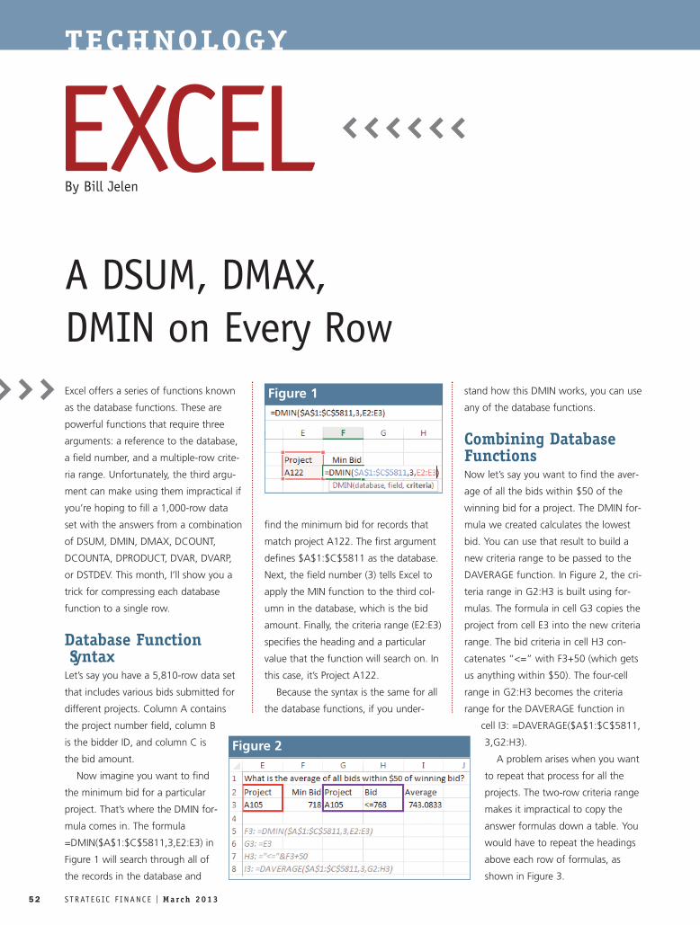
Now imagine you want to find

the minimum bid for a particular

project. That’s where the DMIN for-

mula comes in. The formula

=DMIN($A$1:$C$5811, 3,E2:E3) in

Figure 1 will search through all of

the records in the database and

find the minimum bid for records that

match project A122. The first argument

defines $A$1:$C$5811 as the database.

Next, the field number (3) tells Excel to

apply the MIN function to the third col-

umn in the database, which is the bid

amount. Finally, the criteria range (E2:E3)

specifies the heading and a particular

value that the function will search on. In

this case, it’s Project A122.

Because the syntax is the same for all

the database functions, if you under-

stand how this DMIN works, you can use

any of the database functions.

Combining DatabaseFunctionsNow let’s say you want to find the aver-

age of all the bids within $50 of the

winning bid for a project. The DMIN for-

mula we created calculates the lowest

bid. You can use that result to build a

new criteria range to be passed to the

DAVERAGE function. In Figure 2, the cri-

teria range in G2:H3 is built using for-

mulas. The formula in cell G3 copies the

project from cell E3 into the new criteria

range. The bid criteria in cell H3 con-

catenates “<=” with F3+50 (which gets

us anything within $50). The four-cell

range in G2:H3 becomes the criteria

range for the DAVERAGE function in

cell I3: =DAVERAGE ($A$1: $C$5811,

3,G2:H3).

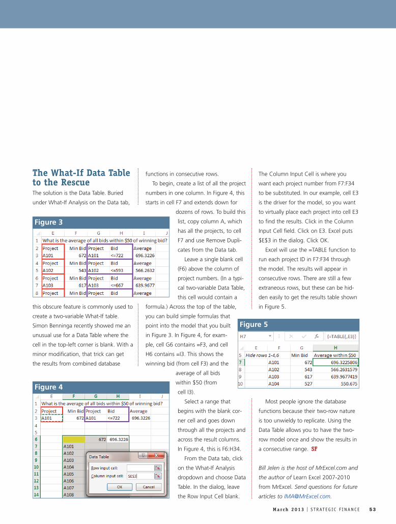
A problem arises when you want

to repeat that process for all the

projects. The two-row criteria range

makes it impractical to copy the

answer formulas down a table. You

would have to repeat the headings

above each row of formulas, as

shown in Figure 3.

TECHNOLOGY

EXCELA DSUM, DMAX, DMIN on Every Row

By Bill Jelen

52 S T R AT E G IC F I N A N C E I March 2013

Figure 1

Figure 2

March 2013 I S T R AT E G IC F I N A N C E 53

The What-If Data Tableto the RescueThe solution is the Data Table. Buried

under What-If Analysis on the Data tab,

this obscure feature is commonly used to

create a two-variable What-If table.

Simon Benninga recently showed me an

unusual use for a Data Table where the

cell in the top-left corner is blank. With a

minor modification, that trick can get

the results from combined database

functions in consecutive rows.

To begin, create a list of all the project

numbers in one column. In Figure 4, this

starts in cell F7 and extends down for

dozens of rows. To build this

list, copy column A, which

has all the projects, to cell

F7 and use Remove Dupli-

cates from the Data tab.

Leave a single blank cell

(F6) above the column of

project numbers. (In a typi-

cal two-variable Data Table,

this cell would contain a

formula.) Across the top of the table,

you can build simple formulas that

point into the model that you built

in Figure 3. In Figure 4, for exam-

ple, cell G6 contains =F3, and cell

H6 contains =I3. This shows the

winning bid (from cell F3) and the

average of all bids

within $50 (from

cell I3).

Select a range that

begins with the blank cor-

ner cell and goes down

through all the projects and

across the result columns.

In Figure 4, this is F6:H34.

From the Data tab, click

on the What-If Analysis

dropdown and choose Data

Table. In the dialog, leave

the Row Input Cell blank.

The Column Input Cell is where you

want each project number from F7:F34

to be substituted. In our example, cell E3

is the driver for the model, so you want

to virtually place each project into cell E3

to find the results. Click in the Column

Input Cell field. Click on E3. Excel puts

$E$3 in the dialog. Click OK.

Excel will use the =TABLE function to

run each project ID in F7:F34 through

the model. The results will appear in

consecutive rows. There are still a few

extraneous rows, but these can be hid-

den easily to get the results table shown

in Figure 5.

Most people ignore the database

functions because their two-row nature

is too unwieldy to replicate. Using the

Data Table allows you to have the two-

row model once and show the results in

a consecutive range. SF

Bill Jelen is the host of MrExcel.com and

the author of Learn Excel 2007-2010

from MrExcel. Send questions for future

articles to IMA@MrExcel.com.

Figure 5

Figure 3

Figure 4