Technology Adoption and Dissemination in Agriculture ... · 1 Technology Adoption and Dissemination in Agriculture: Evidence from Sequential Intervention in Maize Production in Uganda

GRIPS Discussion Paper 13-14

Technology Adoption and Dissemination in Agriculture:

Evidence from Sequential Intervention in Maize Production in Uganda

Tomoya Matsumoto

Takashi Yamano

Dick Sserunkuuma

July 2013

National Graduate Institute for Policy Studies

7-22-1 Roppongi, Minato-ku,

Tokyo, Japan 106-8677

1

Technology Adoption and Dissemination in Agriculture:

Evidence from Sequential Intervention in Maize Production in

Uganda

By TOMOYA MATSUMOTO, TAKASHI YAMANO, AND DICK SSERUNKUUMA*

We use a randomized control trial to measure how the free

distribution of modern inputs for maize production affects their

adoption in the subsequent season. Information collected through

sales meetings where modern inputs were sold revealed that the

average purchase quantity of free-input recipients was much higher

than that of non-recipients; that of the neighbors of recipients fell

in-between. Also, credit sales had a large impact on purchase

quantity, and the yield performance of plots where the free inputs

had been applied positively affected the purchase quantities of both

recipients and the neighbors with whom they shared information on

farming. (JEL O13, O33, O55)

* Matsumoto: National Graduate Institute for Policy Studies, 7-22-1 Roppongi, Minato-ku, Tokyo 106-8677, Japan and

International Livestock Research Institute, P.O.Box 30709-00100, Nairobi, Kenya (email: [email protected]);

Yamano: National Graduate Institute for Policy Studies, Tokyo, Japan and International Rice Research Institute, 1st Floor,

CG Block, NASC Complex, Dev Prakash Shastri Marg, Pusa, New Delhi-110012, India (email: [email protected]);

Sserunkuuma: Makerere University, P.O.Box 7062, Kampala, Uganda (email: [email protected]). For their

2

excellent comments on a previous draft of this paper, we wish to thank Masayuki Kudamatsu and the participants of the

World Bank ABCDE conference in Stockholm, May 2010; Yutaka Arimoto, Takashi Kurosaki, and the participants of the

Japan Economic Association Conference, June 2010; William Master, Christopher Udry and the participants of the African

Economic Research Consortium Workshop in Mombasa, December 2010; Munenobu Ikegami and the participants of the

Brookings Institution Africa Growth Forum, January 2011; and Andrew Zeitlin and the participants of the Oxford CSAE

Conference, March 2011. We also thank George Sentumbwe, Geoffrey Kiguli, and other research team members from

Makerere University who contributed to the project. We are grateful for funding from the Global COE project, sponsored

by the Ministry of Education, Culture, Sports, Science, and Technology, Japan.

Why are the adoption rates of modern agricultural inputs such as hybrid seed

and chemical fertilizers so low in developing countries? This is an empirical

puzzle that relates to technology adoption in agriculture. In Sub-Sahara Africa in

particular, the adoption rate and application level of agricultural modern inputs

have been very low. Despite the presence of large-scale public interventions that

encourage farmers to use such technologies and boost agricultural productivity,

their proliferation has been slow and incomplete; hence, agricultural productivity

in this region has been stagnant for several decades.1

This study examines technology adoption and dissemination in terms of maize

production in Uganda, where the dissemination of technologies relating to

intensive farming methods is in its nascent stage. Technologies for maize

production, more concretely, modern inputs such as chemical fertilizers and

hybrid seeds have been rarely used in Uganda by small-scale farmers. However,

1 Morris, Kelly, Kopicki, and Byerlee (2007) provide a comprehensive review of public interventions geared toward the

promotion of fertilizer use in Sub-Sahara Africa, as well as the consequences thereof.

3

observing recent drastic changes in market and production environment, for

instance, land scarcity due to population pressure, hike in crop prices,

improvement of access to commodity markets and market information; it seems

that Ugandan farmers are facing the onset of transition from traditional to modern

farming system.

A situation in which there is potential demand for inputs but those inputs are

not well-known to farmers is ideal for us in examining farmers’ adoption behavior

of new agricultural technologies and their diffusion. To investigate the impact of a

proposed policy intervention on technology adoption among small-scale farmers,

in 2009, we conducted an experimental intervention in maize production in

Uganda. The intervention involved a sequential randomized–controlled trial. The

first exercise therein was a village-level randomized control trial, implemented

prior to the first cropping season. We distributed free maize inputs and gave 2

hours of instruction on the use of those inputs. We targeted households located in

46 treatment villages, randomly selected from 69 target villages; we asked each

household to allocate a quarter-acre of land as a trial plot where the inputs would

be applied, while we did not do so in the other 23 control villages. The second

exercise of the trial occurred in the intermediate period between the first and

subsequent cropping seasons of 2009, when we revisited the 69 target villages to

sell the same inputs previously provided for free to the sample farmers. We held a

sales meeting in each of the target villages, inviting both the original target

4

households and the neighbors of the free-input recipients in the treatment villages.

The purpose of the workshop was to gather information on input demand for the

participating households and make comparisons among the three groups—the

non-recipients, recipients, and neighbors of the recipients—by actually selling the

modern inputs. In addition to the experimental interventions (i.e., the free-input

distribution and the sales meeting), we conducted the survey in October–

December 2009 to collect information, particularly on the performance of the trial

plots and details of social networking among the participants in the interventions.

Data from both the experimental interventions and the later survey were used in

this study.

The information from the sales meeting showed that (i) the distribution of

modern agricultural inputs has a positive effect on the purchases of farmers with

little experience in the use of inputs; (ii) the intervention had a spillover effect on

the neighbors’ adoption; and (iii) the credit sale option also had a large impact, as

it allowed deferred payment of the input cost after the harvest. The impact of the

credit sales was largest among recipients of the free trial packages.

Moreover, the survey data revealed that there was a high level of heterogeneity

across the recipients, in terms of yield performance of the trial plots where the

distributed inputs were applied. There were some individuals for whom the yield

gain from the use of modern inputs was not sufficiently large to cover the cost of

inputs, although the inputs did help many farmers realize a positive profit. The

5

heterogeneity in the return of inputs in the trial plots enabled us to examine the

intensity of own learning as well as social learning related to the performance of

the modern inputs.

Among the recipients, the yield gain from the modern inputs, measured by the

difference between the actual yield of the trial plot and the hypothetical yield of

traditional farming methods predicted by the farmers themselves, positively

affected their purchase quantities. Not surprisingly, a successful experience

tended to increase the farmers’ purchase quantities of modern inputs for the

subsequent season more than an unsuccessful one.

The performance of the trial plots of the recipients of the free inputs also

positively affected the purchase quantities of the neighbors with whom the

recipients shared information on the farming business; on the other hand, it did

not affect the purchase quantities of neighbor households who merely lived in

proximity but did not exchange farming information with the recipients. These

findings suggest that farmers learn new agricultural technologies through social

networking rather than through geographic peers, and that they will adopt such

technologies in cases where they recognize the benefits thereof.

The rest of this paper is organized as follows. Section I reviews the related

literature and background information on the current farming system in Uganda.

Section II discusses a series of interventions that we have conducted in Uganda

since January 2009. Section III discusses the village-level and household-level

6

data comprising the same, by type of household. Section IV reports the key results

of the sales experiment and yield predictions based on the quantities of modern

agricultural inputs purchased at the sales experiment. Finally, Section V

concludes the paper.

I. Background

A. Related literature

There has been a growing body of empirical literature on technology adoption

in agriculture in Africa.2 There is little doubt that there are profitable agricultural

technologies suitable to conditions in Africa. Many studies confirm the high

average return of agricultural inputs or methods, for example, fertilizers for maize

production in Kenya (Duflo, Kremer, and Robinson (2008)) and hybid seeds in

Kenya ( ri ( )), fertili ers for cocoa prod ction in hana ( eitlin, aria,

ene, ans , po , and eal ( )), and the s stem of rice intensification

(SRI) method for rice production in Madagascar (Moser and Barret (2006)).

Nonetheless, such technologies tend to diffuse slowly and incompletely. This

2 The literature on technology adoption in agriculture is reviewed comprehensively by Sunding and Zilberman (2001)

and Feder, Just, and Zilberman (1985). Foster and Rosenzweig (2010) review more recent literature in technology adoption

in general, and Munshi (2008) reviews literature on social learning.

7

observation constitutes a puzzle in Africa, if one considers the low rate of

adoption of technologies that offer the promise of high returns.

In the case of Uganda, evidence of the profitability of modern agricultural

inputs is sporadic, and some of the available estimates are conflicting. The results

of trial plots for experimental purposes indicate the very high physical returns of

modern inputs. For instance, based on a report by the National Agricultural

Research Organization (NARO) in Uganda, the difference in average crop yields

between NARO trial stations that use modern inputs and the plots of local farmers

who typically use no modern inputs shows a considerable physical yield response

to the inputs, indicating large potential profits (Bayite-Kasule (2009)). Namazzi

(2008) reports the results of fertilizer response trials on maize that were carried

out in 2003 across different districts by Sasakawa Global 2000, an international

nongovernmental organization that promotes agricultural technologies in several

African countries; that study shows that fertilizer application was generally high

and profitable, although the level of profitability varied by region.

Unlike the reports from the trial plots, the results of local farmer surveys tend to

be quite varied. Matsumoto and Yamano (2009) estimate the maize yield function,

using plot-level panel data from 2003 and 2005; they compare the marginal

physical product of inorganic fertilizer with its relative price to maize grain, and

conclude that the relative price is too high for the average farmer to turn a profit

from the use of fertilizer. Nkonya, Pender, Kaizzi, Kato, and Mugarura (2005)

8

also report that the use of inorganic fertilizer appears not to be profitable for most

farmers, based on the results of their farm household survey.

he inp ts’ low average economic ret rn on the gro nd does not necessaril

mean that such technologies are not profitable to all farmers who face different

weather, soil, and market-access conditions, given the high performance of

modern inputs in demonstration plots. Returns could vary among regions and

even individuals, depending not only on their environment and conditions but also

on their knowledge of how to use the technologies. Several recent studies point

out the importance of heterogeneous returns to agricultural technologies, to

understand the reasons of low adoption rate of technologies that have high

average expected returns. Suri (2011) argues, in her study of maize production

that covers most of the maize-growing areas in Kenya, that the low adoption rate

of modern inputs can be accounted for by the heterogeneity of returns to modern

inputs.3 That is, although the average ret rn is high, the ret rn differs largel

across regions, individ als, and time, and hence, some farmers do not se them

persistentl eitlin, aria, ene, ans , po , and eal ( ) also report

that the high average effect of modern inputs on cocoa production among Ghanian

farmers were found to be consistent with negative economic profits, for a

3 Duflo, Kremer, and Robinson (2008) also found that the returns of inorganic fertilizer in maize production varied

across farmers in western Kenya.

9

substantial fraction of the farmers who were provided a package of fertilizer and

other inputs on credit.

In our experimental setting, the modern inputs distributed to farmers for the

purpose of their trial were not tailored, and instruction on usage delivered to

farmers in the training workshop was uniform across all villages and participants.

Given heterogeneous agricultural and market conditions, we expected that the

non-tailored inputs would create variations in return across villages and even

individuals within a village. Thus, in addition to the average effect of an

intervention that involves the introduction of new inputs, we also focus in the

following section on measuring the effect of heterogeneous returns on adoption

and assess whether differences in returns are related to the adoption of the inputs

in the subsequent season.

Our study also looks to measure the effect of social learning. Recent literature

on technology adoption often uses experiments to measure social-learning effects

(Kremer and Miguel (2007), Duflo, Kremer, and Robinson (2011), Dupas (2010)).

Experimental approaches can overcome the reflection problem that arises when

inferring that the adoption behavior of individuals is due to other reference group

members’ adoption—behavior that could be due, in turn, to the presence of

common unobservable characteristics that also affect all member adoption

(Manski (1993)). Using an experimental approach, researchers can create an

exogenous variation in distribution that determines whether or not experiment

10

participants are exposed to a new technology in the initial period, whereupon the

researchers can then observe their neighbors’ adoption in subsequent periods. Our

study is within this domain.

The social-learning effect was measured by comparing the purchase quantities

of the modern inputs between the neighbors of the recipients of free inputs and

those who lived in the control villages. We found large positive effects, which is

not consistent with the findings of Duflo, Kremer, and Robinson (2011) or Suri

(2011), each of who found little evidence of social learning in modern inputs for

maize production among Kenyan farmers. An important difference between these

studies and ours is that the technologies addressed (i.e., hybrid seed and chemical

fertilizers) are not new to Kenyan farmers, but are new to Ugandan farmers. In

Kenya, these technologies have been known to most farmers for many years (Suri

(2011)); in our sample in Uganda, however, only 10 percent of households had

reported experience in the use of hybrid seed before our intervention, and a

negligible number of households had used chemical fertilizers in crop production.

Unlike Uganda, there might be nothing new or easy to learn from others at this

stage of the diffusion process in Kenya. Thus, once we consider the difference in

the degree of dissemination between these two countries, the difference in impact

as a result of social learning, with respect to these technologies, will be more

readily comprehended.

11

In addition to the experiment, during the first intervention, we collected detailed

information regarding social networks from the neighbors of the recipients of the

free inputs. Using this information, we disting ished learning from “geographic

peers” who live in geographical proximit from that of “information peers” who

exchange farming business information. We found that the performance of the

trial plots of the recipients also positively affected the purchase quantities of the

information peers, but that it did not affect the purchase quantities of the

geographic peers. This finding is consistent with that of a recent study by Conley

and Udry (2010), who argue that it is not geographical proximity but rather

information networks that significantly enhance social learning.

B. Maize production in Uganda

In Africa, the application level of chemical fertilizers and the adoption rate of

high-yielding varieties are generally much lower than in other parts of the world.

However, there are also large variations across African countries. One example

can be seen in the interesting contrast in the use of modern inputs for maize

production between two neighboring countries, Kenya and Uganda (Matsumoto

and Yamano (2009)). Only a few farmers in Uganda have used modern inputs in

maize production while most farmers in Kenya have used them for long.

12

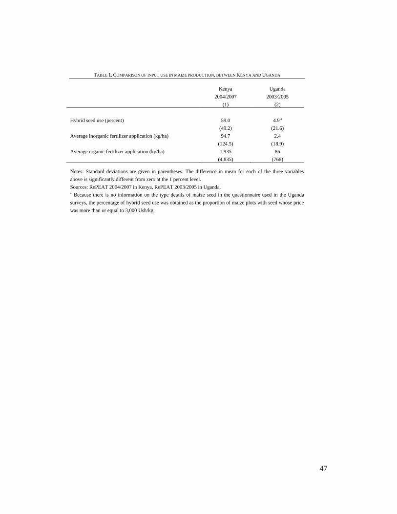
Table 1 compares input use for maize production between Kenya and Uganda,

using data from the RePEAT surveys in Kenya and Uganda.4 In the survey years,

only 5 percent of farmers in Uganda planted hybrid maize seed, and they applied

negligible amounts of chemical and organic fertilizers on the maize plots. In

contrast, about 60 percent of Kenyan farmers planted hybrid seed and used 94

kg/ha of chemical fertilizers; in addition, they used more than 1 ton/ha of organic

fertilizers on maize plots. Some of the farmers in Kenya have been using such

inputs for a decade or longer, and most of them have at least some experience

with them.5 As a consequence, the average maize yield is higher in Kenya than in

Uganda.

[ Insert Table 1 Here ]

Owing to the high transportation costs associated with the import of modern

inputs, particularly in Uganda, the market price of those inputs is high, and hence

their profitability is low (Omamo (2003)). As standard neoclassical models of

4 RePEAT (Research on Poverty, Environment, and Agricultural Technologies) is a research project headed by a

research team of the National Graduate Institute for Policy Studies (GRIPS) and the Foundation for Advanced Studies on

International Development (FASID, Japan). It aims to identify constraints and effective technologies that reduce poverty in

east African countries—especially Kenya, Uganda, and Ethiopia—through empirical analyses based on field data vis-à-vis

agricultural production, collected from farm households. RePEAT also indicates their intention to repeat data collection, in

order to construct panel data over a longer period. (See Yamano, et al. (2004) for more details.)

5 The RePEAT surveys in Kenya mainly covered areas in the Central, Rift Valley, Nyaza, and Western provinces,

where population density is higher and the environment is better suited to crop production than other areas.

13

technology adoption predict,6 the low profitability of modern inputs has been one

of the major reasons for low adoption rates and application levels among Ugandan

farmers. In addition, in the past, the issue of land scarcity was not a prominent one

in Uganda, owing to favorable climate conditions for crop production relative to

the population densities of the country. Thus, Ugandan farmers have had little

incentive to use modern inputs for intensive farming. Moreover, because of the

low potential demand for these inputs, the supply network in Uganda has not been

adequately developed to make their use financially feasible.

However, conditions for farming have been changing drastically in Uganda.

First, because of high population pressures7 and limitations for the expansion of

arable land through land-clearing, land is becoming increasingly scarce; as a

result, the average amount of land per household has been decreasing rapidly

(National Environment Management Authority (2007)). Second, recent hikes in

crop prices are prompting farmers to change their perceptions with regard to crop

production. Some farmers have started to consider crop production a business

enterprise rather than purely for subsistence. Third, owing to infrastructure

6 See, for instance, Besley and Case (1993) and Munshi (2004) with regard to the model for learning about the

profitability of new technologies, and Foster and Rosenzweig (1995) and Conley and Udry (2010) with regard to the model

for learning about the management of new technologies.

7 Estimates of annual population growth rate in 2005 placed Uganda in 11th place worldwide (3.58%) and Kenya in

42nd place (2.36%).

14

improvements such as roads and mobile networks, farmers have had better access

to commodity markets and market information than before.8 These factors have

created high potential demand for intensive farming methods among crop farmers

in Uganda. Since these modern inputs are experience goods, a lack of knowledge

on their usage and profitability might be a large deterrent to their adoption by

farmers who have little experience. Thus, we expected that small interventions

involving one-time material support and training on the usage of such modern

agricultural inputs would have a large impact on their adoption among Ugandan

farmers in the long term.

II. Experimental Design and Survey Data

To investigate the impact of a possible policy intervention on technology

adoption by small-scale Ugandan farmers, we conducted an experimental

intervention there in maize production, in 2009.9

The intervention was a

8 M to and Yamano ( 9) show that the expansion of mobile networ s has ind ced farmers’ mar et participation in

Uganda.

9 The experimental intervention was carried out as part of the Global Center of Excellence (GCOE) Project of GRIPS,

Japan, in collaboration with Makerere University, Uganda. It was financially supported by Ministry of Education, Culture,

Sports, Science, and Technology, Japan.

15

sequential randomized–controlled trial.10

The target sites and individuals were

the sample villages and households in the Eastern and Central regions surveyed

for the RePEAT panel study.11

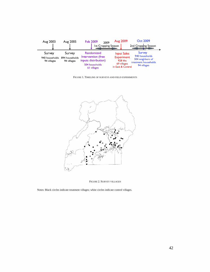
[ Insert Figure 1 Here ]

A. Free-input distribution

In the first exercise, which took place in February and March 2009, prior to the

first cropping season, we distributed free maize inputs to 377 RePEAT

households and asked them to allocate a quarter-acre of land (approximately 0.1

ha) as a trial plot where the inputs would be applied. These households are located

within 46 villages (26 and 20 in the Eastern and Central regions, respectively) that

were randomly chosen from the RePEAT villages.12

For convenience, we refer to

10 Figure 1 shows the timeline for and the number of sample households involved in each project within the RePEAT

study. In the initial RePEAT household survey in 2003, 10 households were surveyed in each village. Because of attrition,

106 households dropped out from the 61 treatment villages.

11 Three of the 94 RePEAT survey villages are excluded from this experimental intervention. Two of them are located

in Kapchowa district, close to the Kenyan border. Their application rates of chemical fertilizers and their adoption rates of

hybrid maize seed, according to the 2005 RePEAT survey, were exceptionally high. The other village has been involved in

the United Nations’ Millenni m Village Project since 8 hese villages are ver different from others in terms of their

experience with modern inputs, and they were thus excluded as unrepresentative outliers.

12 he smallest local administrative nit in Uganda is L In this paper, we refer to the L as a “village ” We

included in the free-input distribution 22 villages (15 treatment and seven control villages) in the Western region. However,

16

the ho seholds in the 46 villages as the “treatment ho seholds”13

; this

distinguishes them from the remaining households located in the other 23 villages

(13 and 10 in the Eastern and Central regions, respectively) that are referred to as

the “control ho seholds ”14

The geographic distribution of those villages is shown

in Figure 2. The randomization for the selection of the treatment villages was

implemented based on a computer-generated random number after the

stratification by region.

[ Insert Figure 2 Here ]

The free inputs distributed to the treatment households were uniform (i.e., non-

tailored) across the treatment villages. They comprised 2.5 kg of hybrid seed, 12.5

kg of base fertilizer, and 10 kg of top-dressing fertilizer.15

In addition, a 2-hour

they were excluded from the second exercise because of time and budget constraints. Thus, in this study, we focus on

samples only from the Eastern and Central regions.

13 There were a small number of households who were part of the original RePEAT sample and invited to the

workshop where free inputs were distributed but did not attend and hence did not obtain them. We also call these

ho seholds “treatment ho seholds ” h s, the treatment ho seholds can be considered part of an “intent to treat” sample

14 We included in the free-input distribution 22 villages (15 treatment and seven control villages) in the Western region.

However, they were excluded from the second exercise because of time and budget constraints. Thus, in this study, we

focus on samples only from the Eastern and Central regions.

15 These are the recommended input levels for growing a quarter-acre of maize by an agronomist in National

Agricultural Research Organization, Namulonge, Uganda just for a research purpose for us to implement an uniform

17

training session on the use of these modern inputs was delivered by an extension

worker to the members of the treatment households.

B. Sales experiment

The second exercise occurred in August and September 2009—the intermediate

period between the first and subsequent cropping seasons—during which we

revisited 46 treatment and 23 control villages in the Eastern and Central regions to

sell the same inputs that had previously been provided for free to the sample

farmers. We held a sales meeting in each of the target villages and invited

members of all the RePEAT households, as well as randomly selected neighbors

of the treatment ho seholds (called “neighbor ho seholds,” hereafter) o select

the neighbor households, we visited each of the treatment households prior to the

sales experiment, asked the household head to list five to 10 households as

neighbors, and then randomly selected one household from the list as the

“neighbor ho sehold ” We expected this neighbor-household selection procedure

to mitigate the selection bias that would occur if the treatment households were to

invite households with special interests or relationships (e.g., friends or relatives),

intervention. The composition may not be optimal under some circumstances because it does not consider heterogeneity of

agroclimatic environments as well as input-output price ratio. The market value of these inputs was 52,500 Ugandan

Shillings (Ush) (US$26.80, at the exchange rate of February 2009).

18

especially, in cases where the treatment households perceived our first

intervention to be beneficial.

We held the sales meeting and provided the supplies procured from a whole

seller in Kampala by ourselves, rather than working with local input suppliers.

This was because the supply network of agricultural inputs had not been well

developed and hence there were places in our target areas where we could not

procure the reliable quality inputs from local retailers.

The purpose of the sales experiment was to gather information on input demand

for the participating households and to make comparisons among the three

groups—the control, treatment, and neighbor households. To obtain information

on their demand in response to a change in price, we sed a “price contingent

order form” that as ed farmers how m ch of each inp t the wo ld b at

different discount levels (Appendix). Three discount rates from the market price

were offered, namely, 0, 10, and 20 percent.16

Which discount rate would be used

for the actual sales was not determined until they filled out the order form,

although the participants were informed at the beginning of the sales experiment

that one of the discount rates would be randomly chosen and that they would need

to pay for the amounts indicated on the form at the chosen discounted price.

16 We were interested in collecting information on the purchase quantities at a wider range of discount rates. However,

given the possibility that the participants could profit from reselling inputs to other residents or even input dealers, we

could not offer higher discount rates.

19

We used a similar order form for credit purchases, on which participants

indicated how much of each input they would buy if credit were available. In the

proposed credit scheme, the participants were allowed to pay the balance—that is,

the total payment with interest, minus the initial payment—at the end of the

subsequent season after the harvest, as long as the initial payment exceeded the

minimum down-payment agreed upon at the meeting. The interest rate and the

minimum down-payment rate were randomly assigned at the village level,

according to the project. The interest rates offered were 5, 10, or 15 percent per

cropping season. The minimum down payments offered were 20, 30, or 40

percent.

After the participants filled out the forms, one of them—typically a village

leader—drew a ball from a bingo cage to randomly determine the discount rate; a

second ball was then drawn, to determine whether the credit option was actually

available to the group. The chance of winning the credit option was one in 10.17

Finally, at the end of the sales experiment, the participants did, in fact, purchase

inputs as indicated on the order forms at the discount level, and with or without

the credit option as determined by the bingo game.

Using the price contingent order form at the sales meeting, we obtained

information on the participants’ p rchase q antit levels at three different

17 The participants in all the 69 villages where the sales experiment was held had a chance to buy inputs on credit.

20

discount rates, with and without the credit option—that is, six quantity levels in

total, for each input from each participant.

C. Survey data

In addition to the experimental intervention, we conducted a survey (called

“RePEA 9,” hereafter) in ctober–December of 2009 and collected

information from the target households. In particular, we collected detailed

information on maize production in the years 2008 and 2009, including that on

input use on the experimental plots and other plots. In addition, we gathered

information on social networks from neighbor households, by using a preprinted

list of the names of the treatment households in the same village, together with the

questionnaire, which asked the neighbor households about their relationship with

each of the treatment households.18

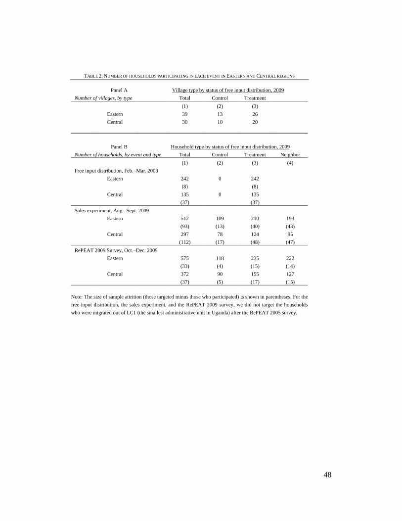
For this study, we used both the data from the

experimental intervention and the survey data conducted later. Table 2 shows the

number of sample villages and households for each event, by region and type of

household.


18 This is useful information in learning about social networks, not only for the neighbor households but also for the

other types of households. However, we were able to collect information only from the neighbor households, given time

and budget constraints regarding the field survey, as data collection had been time-consuming.

21

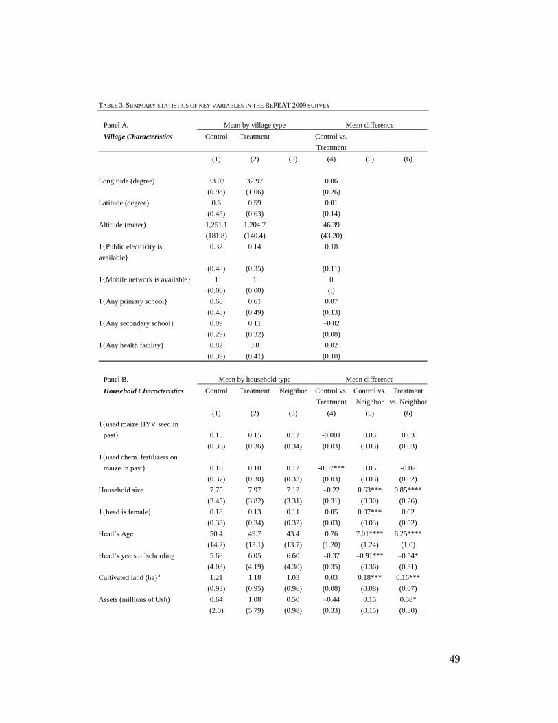
D. Village and household characteristics in 2009

Table 3 shows the characteristics of villages involved in the RePEAT 2009

survey, by village type. Owing to the nature of the random assignment of free-

input distribution, there were presumably no systematic differences in terms of

pre-intervention characteristics, between these types of villages. The test statistics

of the difference in mean of the key variables shown in Column 4 confirmed this

presumption. Similarly, Table 3 shows household characteristics, by household

type. As expected, there were no systematic differences between the treatment

and control households except the past use of chemical fertilizers on maize plots.

(The test statistics of the mean difference are given in Column 4.) The past use of

chemical fertilizers was higher for the control households than the treatment

households. If it had a positive effect on the adoption of modern inputs, we would

underestimate the treatment effect of our intervention without controlling for this

variable. We may need careful investigation on this.

Our sample households comprised small-scale farmers; on average, each

cultivated 1.2 ha of land, contained slightly fewer than eight family members, and

had a head who was 50 years old and had six years of schooling.


22

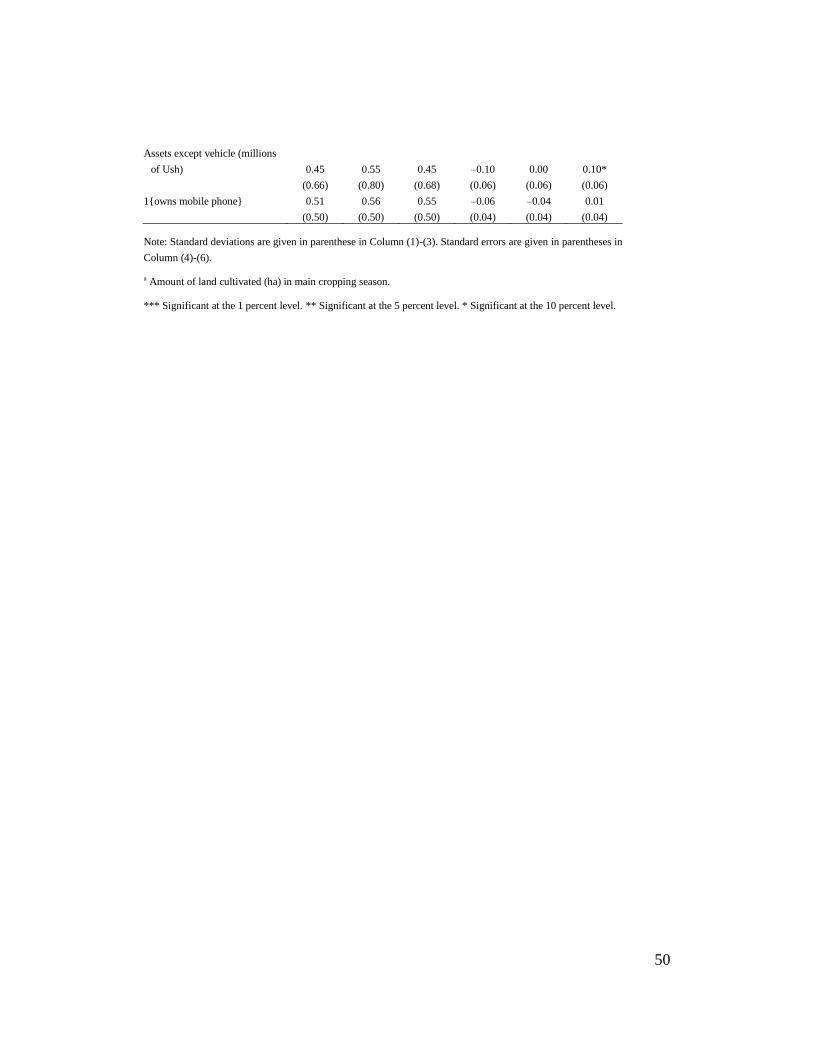
Compared to the treatment and control households, the neighbor households

were smaller in family size and in the land size cultivated; their heads were both

younger and more educated. These differences between neighbor households and

others, despite the sampling scheme (see the explanation of the sales experiment

in the previous section), are probably because the treatment and control

households were already older than the average residents were, because the

original RePEAT samples had been sampled since 2003. At the same time, it may

imply that they are different in their potential demand for intensive farming

methods, owing to differences in land availability and education level. We

controlled for these factors in regressions, to mitigate potential sampling biases

between neighbor households and other types of households.

E. Sample Attritions

In the following analyses, we mainly use the information obtained from the

sales experiment in 2009 and combined with RePEAT 2009 Survey data. There is

an issue to be considered. The sample attritions in the sales experiment are not

negligible, which are indicated in the parentheses in Table 2. When we held the

sales experiment, we announced village leaders (who were supposed not to be the

subject households) about our visit and its purpose two to three weeks prior to the

scheduled date via mobile phone and asked them to circulate the information to

the target households. Then, we also asked the leaders to mention to the target

23

households about the compensation for the participation. However, some of the

target sample households did not show up at the sales experiment because some

might not have been interested in the experiment or other may not have been

correctly informed about the purpose and venue of the sales experiment. As a

consequence, the sample attrition in the sales experiment was large and may cause

a serious selection bias when we estimate the demand curves in the following

analyses. Especially, if those who were not interested in the modern inputs did not

participate in the event, the estimates of the demand for the modern inputs based

only on the participants' information would be upwardly biased.

One simple compromise may be to consider those absentees as those who

would not purchase any input even when they had participated in and to

incorporate them into the samples for the estimation of the demand. In that case,

the purchase quantity of the absentees is set at zero and hence the estimates of the

demand can be considered as the lower bound. We confirmed that the inclusion of

the absentees by setting their purchase quantity at zero did not affect results much

compared with the ones presented in the tables for the following analyses.19

19 Those results will be presented by the author upon request.

24

III. Empirical Strategies

A. Demand for inputs, by household type

The simplest approach to observing the impact of free-input distribution on

adoption behavior on modern inputs in the subsequent season is to compare the

mean values of the purchase quantities at the sales experiment among the different

household types. For convenience, let us denote as the purchase quantity of the

i-th household. Let , , and be the sets of households that belong to the

treatment, control, and neighbor household groups, respectively. Since the

assignment of the treatment status was random, the average effect of the free-

input distribution on the purchase quantity is given simply by

. Also, its effect on the purchase quantity of the

neighbor households is given as .

Since we collected purchase-quantity data with and without the credit option,

we were also able to determine the effect of the credit option on the purchase

quantity by household type, i.e., – for

O , where CR is a binary variable that takes the value of 1 if the credit

option is available, and 0 otherwise.

25

B. Regressions

In addition to the average intervention effect, depending on the ho sehold’s

treatment status, we were also interested in the influence of other factors; which

we examined by using simple regression models. This might also be important in

estimating the impact of the intervention—especiall on the neighbors’ adoption,

given the difference in some characteristics of the neighbor households, compared

to other household types.

First, we considered a model that identified the factors that affect the purchase

quantity of input x of household i located in community j at price level P, as well

as the availability of the credit option, denoted by the dummy variable CR:

(1)

,

where T is a dummy variable for the treatment households, N is a dummy variable

for the neighbor households, and X is a vector of other exogenous variables

associated with the household and the community. The following variables are

considered the exogenous X: the down-payment rate that determined the level of

minimum payment for the credit sales, the interest rate charged for the credit sales,

and their interactions with the credit-sales dummy; the household variables

26

involving the number of family members; the dependency rate (i.e., the ratio of

family members aged below 15 or over 65 to those aged between 15 and 65

inclusively); a dummy variable for female-headed households; the household

head’s age and ears of schooling; the size of land owned in ha; assets-holding

level, in millions of Ush; past use of maize hybrid seed; and past use of chemical

fertilizers on maize production.

C. Heterogeneity in yield and profitability across regions and individuals

The performance of modern inputs used in the trial plots of the treatment

households varied across communities, as well as across households within a

given community. According to the simple learning model, it is expected that

successful experiences from the use of a new technology will enhance the

likelihood of its use in subsequent periods, while unsuccessful experiences will

red ce it In addition to learning from one’s own experiences, the model also

predicts learning from peers—especially among those who share information

(Conley and Udry (2010)). Using survey data collected after the sales experiment,

we examined the effect of the difference in performance of the trial plots on

adoption in the subsequent season.

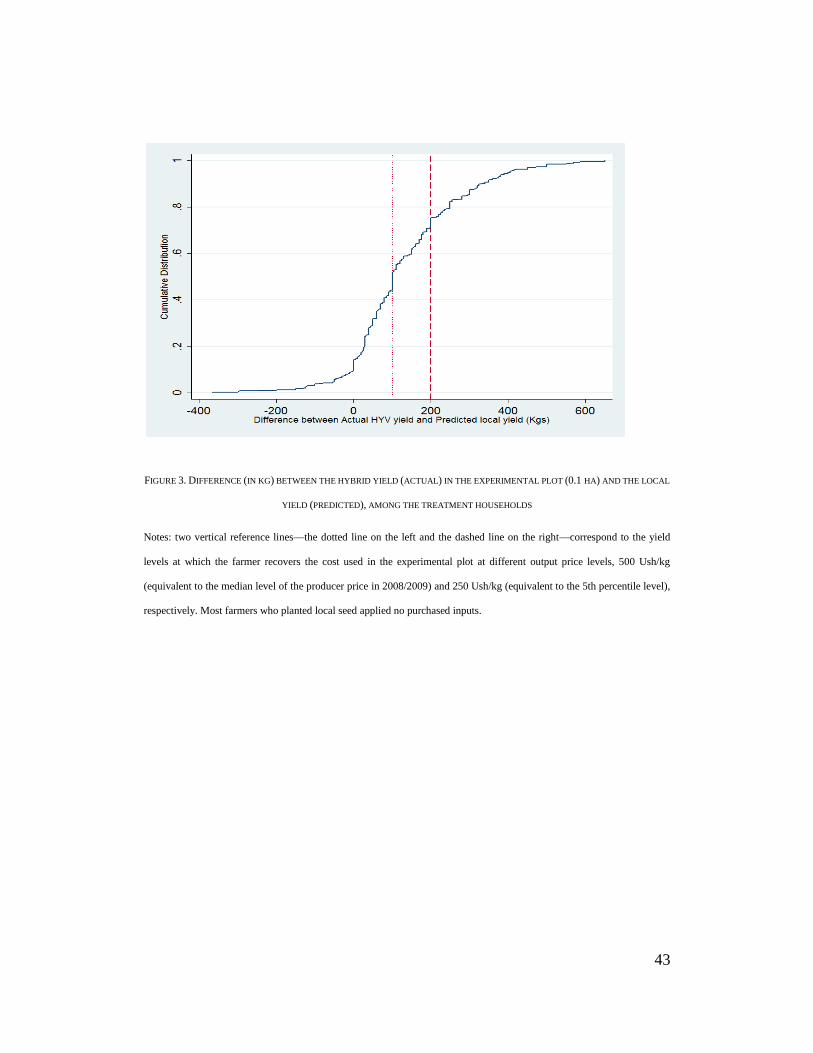
Figure 3 shows the distribution of the yield difference between the actual yield

of the trial plot and the hypothetical yield predicted by the farmers themselves

among the treatment households, had the traditional method been applied to the

27

same plot.20

The two vertical lines indicate the level of yield gain from the use of

modern inputs that would be required to recover the input costs for the trial plot

(approximately US$25) at two different prices of the output. The dotted line

corresponds to the required level at the output price of 500 Ush which is

equivalent to the median producer price in 2008/2009, while the dashed line

corresponds to the level at 250 Ush equivalent to the 5th percentile level.21

Yield

gains varied across individuals, and not all the farmers saw positive profit-gains

from the use of modern inputs. One of the reasons would be the fact that the

modern inputs that we distributed for free had not been tailored to specific regions

or individuals: they may not be suitable for certain soil or climate conditions. Also,

differences in yield gain could be caused by differences in crop management, as

some individuals might have managed them properly, while others did not.

[ Insert Figure 3 Here]

20 There are 203 households which reported both the hypothetical yield and the actual yield of a plot where local seeds

and no fertilizers were applied in the first cropping season in 2009. Comparing the hypothetical yield with the actual yield,

their distributions appeared to be similar; the p-value of the t-test for the difference in mean is 0.895, which cannot reject

the null hypothesis that the difference is equal to zero.

21 Typically, almost no purchased inputs are applied when local seed is planted.

28

D. Learning from one’s own experience: effect among treatment households

Given the large heterogeneity in performance of the modern inputs on the trial

plots, we were able to see its effect on the purchase of the modern inputs during

the sales meeting among the treatment households. We incorporated the yield gain

from the modern input use denoted, where represents the

actual yield from the trial plot (the subscript i corresponds to household i and the

superscript H indicates the use of hybrid seed and chemical fertilizers); ,

meanwhile, is the hypothetical yield reported by household i, had a local seed

variety and no fertilizers been applied in the same plot. We used this variable as a

covariate in the regression of the purchase of modern inputs. In this analysis, we

focused on within-community variations in yield gain as a determinant of the

purchase quantities, by controlling for household-level characteristics X and

community-level specific factors by the community fixed effect .

(2) .

The coefficient β captures the magnitude of the impact of the yield gain (in kg) of

the trial plot from the use of modern inputs on the purchase quantity (in kg). We

estimated the parameters of this model by applying a community-level fixed-

effect regression.

29

E. Learning from peers: effect among neighbor households

Through social networking, the performance of the trial plots would affect

adoption behavior, not only to treatment households themselves but also to their

neighbor households. As Conley and Udry (2010) suggest, the flow of useful

information may not necessarily be restricted to neighbors in close geographic

proximity. Rather, social networks based on friendship or kinship may play

critical roles in diffusing information. In this study, we look to distinguish the

influence of geographic versus information peers.

In the survey following the sales experiment, we collected from neighbor

households data indicating their relationship with each of the treatment

households. Particularly, we used information pertaining to whether or not they

exchanged information on the farming business with each of the treatment

households; we did so, to construct a measure that represents the effect of the

performance of treatment peers’ experimental plots on the decision-making of

neighbor households. We created a variable representing the average of the yield

gain ΔY of the treatment households with which the i-th neighbor household

exchanged information on the farming business, denoted by and referred

to as “mean ield gain of information peers” in the res lts table ( able 7) For the

purpose of comparison, we also constructed the mean yield gain of geographic

30

peers, , which is defined as the weighted average of ΔY of geographic

peers.22

(3) , (n = info or

geo)

The coefficient β captures the magnitude of the impact of the mean yield gain of

peers (in kg) on the purchase quantity (in kg) of the neighbor households. We

estimated the parameters of this model by applying a community-level fixed-

effect regression.

IV. Results

A. Average purchase quantity by household type

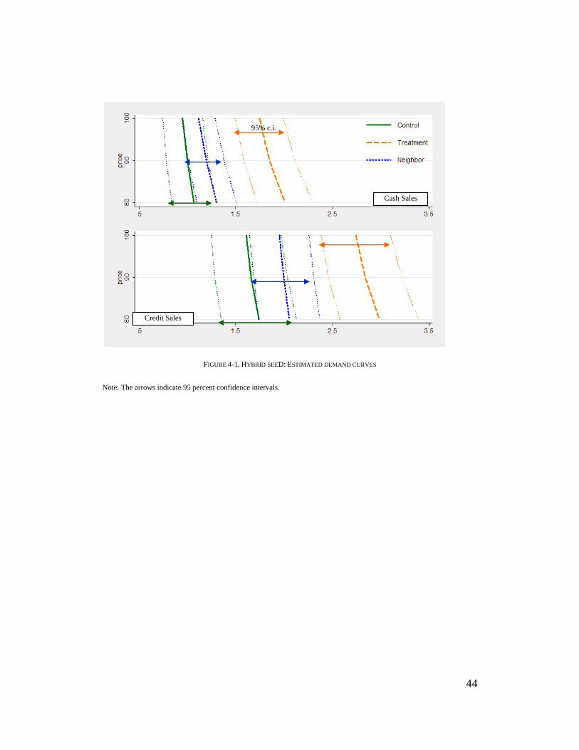
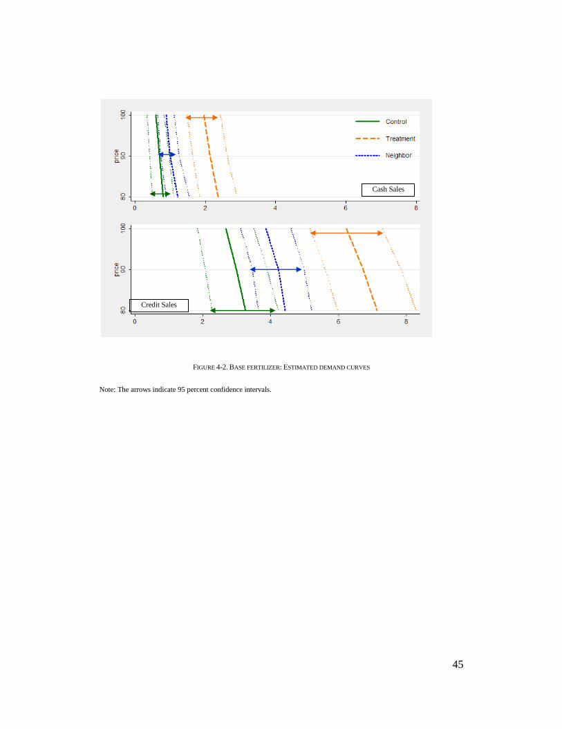
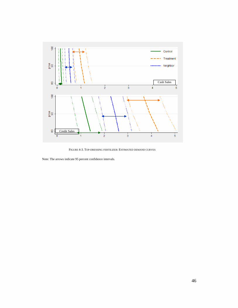
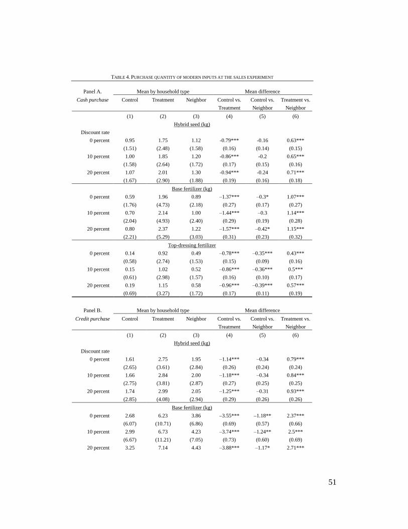
Table 4 shows the results of the average quantity purchased of each input at

different discount rates, by household type.23

Panel A corresponds to the results

22 As the weight, we use the Gaussian kernel, , based on the distance in km between the households.

Thus, the mean yield gain of geographic peers for the i-th neighbor household is given by

where h is a bandwidth. We use h=1.

23 Their graphical representations are give in Figure 4-1 to 4-3, by input type.

31

for cash purchases, and Panel B corresponds to those for credit purchases.

Column 4 in Table 4 reports the difference in mean of purchased quantities

between the control and treatment households and the standard errors of the test

statistics (in parentheses) corresponding to the null hypothesis, in which the

difference in mean is equal to 0. Similarly, Column 5 and 6 show the difference

between the control and neighbor households and the difference between the

treatment and control households, respectively.

[ Insert Table 4 Here]

[ Insert Figure 4-1 Here]



The difference in purchased quantities between the control and treatment

households was statistically significant at the 1 percent level for all inputs and at

all discount levels. This observation confirmed the significant impact of free-input

distribution on the adoption and purchased quantity of modern inputs in the

subsequent cropping season, following free-input distribution. The difference

becomes larger with the availability of credit.

The purchased quantity of modern inputs by neighbor households was larger

than that of control households, in all cases. The difference was statistically

32

significant for chemical fertilizers at all discount levels, but it was not significant

for hybrid seed, as shown in Table 4. The level of purchased quantities lay

between that of control and treatment households, in all cases.

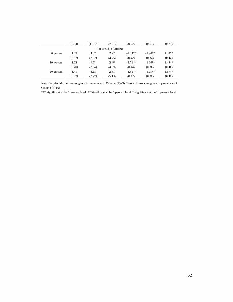
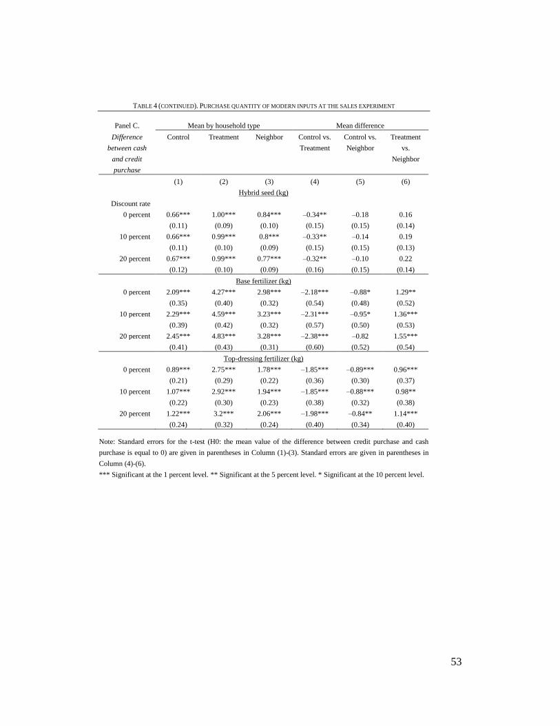
Panel C reports the differences in purchase quantities between the cash and

credit purchase. The effect of credit was very large for all types of households,

especially with regard to fertilizer purchases. The credit option boosted the

purchased quantities of fertilizers more than threefold. The impact of credit was

largest among treatment households, possibly because they had acquired, through

the intervention, knowledge on the usage and profitability of modern inputs.

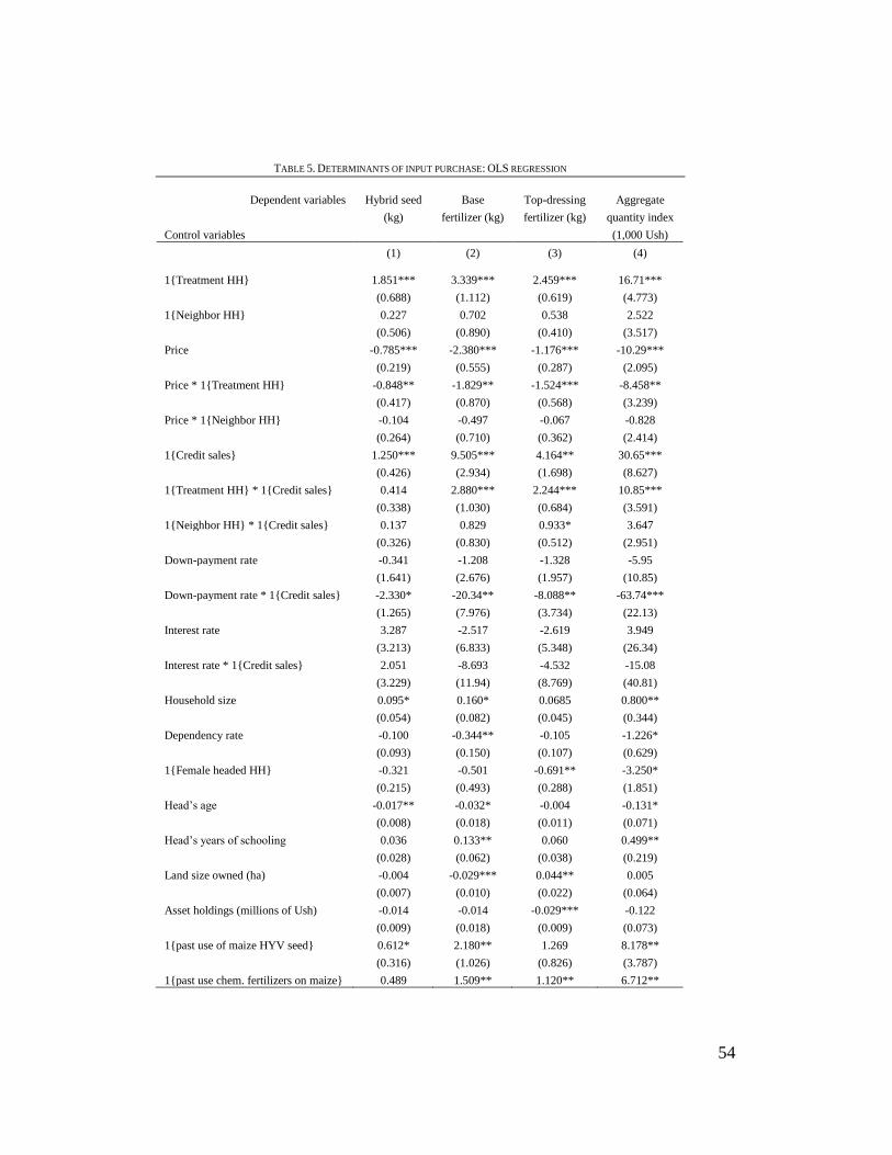
B. Regression results

We considered the four dependent variables for the regressions specified in the

previous section. The first three variables were simply the weight of each of the

three modern inputs—hybrid seed, base fertilizer, and top-dressing fertilizer, in

kilograms—purchased at the sales experiment; the last variable, meanwhile, was

the aggregate quantity index, which is defined as the total cost of those three

inputs at the market price, divided by 1,000.

Table 5 shows the results of the regressions, in which all household types were

used as the sample, corresponding to Eq.(1). The estimates of the coefficients of

the dummy for the treatment households, the neighbor households, and their

interactions with the dummy for the credit option further supported the results of

33

Table 4. The purchase quantity of all the inputs was largest for the treatment

households, and smallest for the control households (reference group); in the

middle were the neighbor households, although the difference between the

neighbor and control households was not significant. The credit option has the

largest impact on all types of inputs. We also confirmed that the credit option had

a differential impact, depending on the household type: it was largest for the

treatment households (which can be seen as the coefficient of the interaction term

of the credit-option dummy with the dummy for the treatment households) and

smallest for the control households. These estimates were consistent with the

results in Table 4, in which only the mean effect of the treatment status was

considered and the other factors ignored; this implies that our randomization had

been successfully implemented.


The minimum down-payment rate—which determines the amount of cash

payment required to be paid during the sales experiment for a credit purchase, and

is randomly assigned at the community level—had a negative impact on the

purchase quantity, but only for credit purchases. This result was consistent with

the fact that the down payment rate was effective only for credit sales. Also, the

significant effect implied that the immediate cash constraint was binding for the

average participant in the sales experiment. A 10 percentage-point increase in the

34

minimum down-payment rate would result in a 6,374 Ush decrease in the total

input purchase.

The interest rate—charged for the cost of credit purchases and randomly

assigned at the community level—was also effective for credit purchases only.

Although we expected it to have a negative impact on the input purchase only for

credit purchases, we obtained a somewhat odd result: the coefficient of the

interest rate was positive and significant for the cash purchase of hybrid seed.

This finding may require further investigation.

Household size had a positive and significant effect on the purchase quantities

of seed and base fertilizer, and on the quantity index. This may suggest that labor

requirements for intensive farming methods that use modern inputs are higher

than those for traditional farming he coefficients of the ho sehold head’s age

were negative and significant, meaning that younger farmers were more active in

the se of new inp ts than older ones he head’s ears of schooling had a

positive effect on the purchase of modern inputs, indicating that more educated

persons were more willing to buy modern inputs, although the magnitude was

relatively small. The coefficients of size of land owned showed inconsistent signs,

depending on the type of inputs. The coefficients of level of asset holdings were

negative for all inputs, although their magnitude, too, was very small.

The coefficients of past use of hybrid seed and chemical fertilizers were

positive for all and significant, except for the purchase quantity of hybrid seed.

35

Although only a few farmers used maize hybrid seed and chemical fertilizers on

maize prior to our experimental intervention (as shown in Table 1), it seems that

they had known of the value of modern inputs and hence purchased more at the

sales experiment.

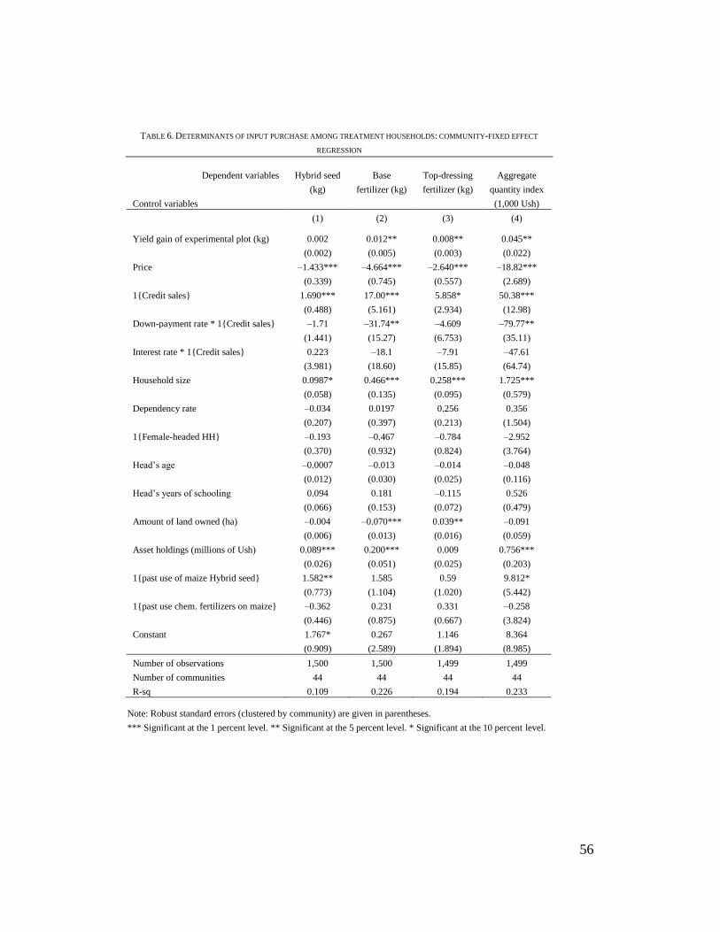
C. Learning from own experience

We focused on the effect, among the treatment households, of the differential

performance of the experimental plots that used modern inputs on purchase

quantities in the subsequent season. Table 6 shows the results of regressions

corresponding to Eq.(2), which helped determine the effects of the performance of

the experimental plots among treatment households.

Yield gains in the experimental plots, which were measured as the difference

between the act al ield of the experiment plot and the farmer’s prediction of the

yield with the use of traditional inputs in the same plot, were found to

significantly increase the purchase of inputs during the sales experiment. For

example, on average, a 100-kg gain—the approximately median gain—increased

the purchase of inputs by 4,510 Ush at the market price during the sales

experiment (Table 6, regression 4). For other covariates, the results were more or

less similar to the previous regressions in Table 5.


36

D. Learning from peers

We estimated the impact of the yield gain of the treatment households on the

neighbor ho seholds’ inp t p rchases We sed two variables defined in the

previous section: the mean yield gain of information peers and the mean yield

gain of geographic peers, in their respective experimental plots. The results are

provided in Table 7. The coefficients of the mean yield gain of the information

peers were all positive and significant, except for that of the top-dressing

fertilizer; those of geographic peers showed different signs, depending on the

types of input measures, and they were not significant for any of the inputs. This

observation suggests that information on the usefulness or profitability of

technology, or modern inputs, flows through an information network more

efficiently than among neighbors with geographic proximity, and hence boosts the

adoption of such technology.


IV. Conclusions

Maize productivity in Uganda remains very low; one obvious reason for this is

the limited use of modern maize inputs. In the early stages of technology

dissemination, a lack of knowledge is a crucial explanation for the low adoption

rate of profitable technologies. Our study results showed that once farmers

37

recognize the benefits of new inputs in crop production, many of them will invest

in the inputs for the subsequent season. It is also important to note that farmers

learn from their own and others’ s ccessful experiences, through social

networking. These observations point to the importance of agricultural extension

services in diffusing new and profitable technologies. Emphasizing the role of

extension services, it is obviously important to note that because the profitability

of a technology can vary to a great extent across regions and with time, an

untailored technology will not bestow benefits upon every farmer in every place.

Technologies may need to be chosen by those with on-the-ground knowledge of

suitable technologies and their profitability. For this reason, it might often be the

case that local private stakeholders such as input suppliers who can both deal with

tailored agricultural-input technologies and have knowledge of the commodity

market might well be more competent providers of extension services than public

providers. We believe that there is ample opportunity for the private sector to play

a significant role in this service area.

Finally, this study also showed that Ugandan farmers face severe credit

constraints; this was underscored by the fact that their demand for inputs

increased significantly when they were given a credit option. This observation

suggests that the provision of affordable financial services in rural areas could

prompt Ugandan farmers to change their farming methods, boost productivity,

and improve their quality of life. Owing to the development of mobile

38

technologies and drastic reductions in the transaction costs associated with

communication and financial services via mobile phones, financial services that

target small-scale farmers in remote areas can become more feasible, at least on a

technical level. The provision of such services promises the potential of great

advances among the farmers in Uganda.

REFERENCES

Bayite-Kas le, , 9 “Inorganic Fertili er in Uganda—Knowledge Gaps,

Profitabilit , bsid , and Implications of a National Polic ,” Uganda trateg

Support Program (USSP) Brief No. 8, International Food Policy Research

Institute, Washington, DC, USA.

Besle , , ase, A , 993 “Modeling echnolog Adoption in eveloping

o ntries,” American Economic Review Papers and Proceedings, 83(2), 396–

402.

onle , Udr , , “Learning Abo t a New echnolog : Pineapple in

Ghana,” American Economic Review, 100(1), 35-69.

flo, E , Kremer, M , Robinson, , 8 “How High Are Rates of Ret rn to

Fertili er? Evidence from Field Experiments in Ken a,” American Economic

Review, 98(2): 482–8.

Duflo, E., Kremer, M., Robinson, J., 2011 “N dging Farmers to Use Fertili er:

heor and Experimental Evidence from Ken a,” American Economic Review,

39

101(6), 2350-90.

pas, P , “ hort-Run Subsidies and Long-Run Adoption of New Health

Prod cts: Evidence from a Field Experiment,” NBER Working Papers, 16298.

Feder, , st, R , ilberman, , 985 “Adoption of Agric lt ral Innovations in

eveloping o ntries: A rve ,” Economic Development and Cultural

Change, 33(2), 255–98.

Foster, A , Rosen weig, M , 995 “Learning b oing and Learning from Others:

H man apital and echnological hange in Agric lt re,” Journal of Political

Economy, 103, 1176–209.

Foster, A , Rosen weig, M , “Microeconomics of echnolog Adoption,”

Annual Review of Economics, 2(1), 395–424.

Kremer, M., Miguel, E , 7 “ he Ill sion of stainabilit ,” Quarterly Journal

of Economics, 122(3): 1007–65.

Mans i, , 993 “Identification of Endogeno s ocial Effects: he Reflection

Problem,” Review of Economic Studies, 60(3): 531–42.

Matsumoto, T., Yamano, T., 2009 “ oil Fertilit , Fertili er, and the Mai e reen

Revol tion in East Africa,” World Bank Policy Research Working Paper, no.

WPS 5158.

Morris, M., Kelly, V.A., Kopicki, R., and Byerlee, D., 2007. Promoting Increased

Fertilizer Use in Africa: Lessons Learned and Good Practice Guidelines.

Washington, DC: World Bank.

40

Moser, Barret 6 “ he omplex namics of mallholder echnolog

Adoption: he ase of RI in Madagascar,” Agricultural Economics, 35, 373–

88.

M nshi, K , 4 “ ocial Learning in a Heterogeneous Population: Technology

iff sion in the Indian reen Revol tion,” Journal of Development Economics

73(1): 185–213.

M nshi, K , 8 “Information Networ s in namic Agrarian Economies,” in

Handbook of Development Economics, Vol. 4. ed. by T.P. Schultz and J.

Strauss. Oxfort: Elsevier Science.

Nama i, , 8 “Use of Inorganic Fertili er in Uganda,” IFPRI-Kampala

Policy Brief.

National Environment Management Authority (NEMA), 2008. State of

Environment Report for Uganda. Kampala: NEMA.

Nkonya, E , Pender, , Kai i, , Kato, E , M gar ra, , 5 “Polic ptions

for Increasing Productivity and Reducing Soil Nutrient Depletion and Poverty

in Uganda,” Environment and Production Technology Division Discussion

Paper, no. 132. International Food Policy Research Institute, Washington, DC,

USA.

mamo, W , 3 “Fertili er rade and Pricing in Uganda,” Agrecon, 42(4),

310–24.

nding, , ilberman, , “ he Agric lt ral Innovation Process:

41

Research and Technology Adoption in a Changing Agric lt ral ector,” in

Handbook of Agricultural Economics, Vol. 1, ed. by B. Gardner and G. Rausser.

Amsterdam: North Holland.

ri, , “ election and omparative Advantage in echnolog Adoption,”

Econometrica, 79(1), 159–209.

Yamano, T., Sserunkuuma, D., Otsuka, K., Omiat, G., Ainembabazi, J.H.,

himam ra, Y , 4 “ he 3 RePEA rve in Uganda: Res lts,”

http://www3.grips.ac.jp/~globalcoe/j/data/repeat/REPEATinUgandaReport.pdf,

accessed September 19, 2011.

Yamano, T., Muto, M., 2009. “ he Impact of Mobile Phone overage Expansion

on Mar et Participation: Panel ata Evidence from Uganda,” World

Development, 37(12), 1887–96.

eitlin, A , aria, A , ene, R , ans , P , po , R , eal, F ,

“Heterogeneo s Ret rns and the Persistence of Agricultural Technology

Adoption,” Centre for the Study of African Economies Working Paper,

WPS/2010‐37, November 2010.

42

FIGURE 1. TIMELINE OF SURVEYS AND FIELD EXPERIMENTS

FIGURE 2. SURVEY VILLAGES

Notes: Black circles indicate treatment villages; white circles indicate control villages.

43

FIGURE 3. DIFFERENCE (IN KG) BETWEEN THE HYBRID YIELD (ACTUAL) IN THE EXPERIMENTAL PLOT (0.1 HA) AND THE LOCAL

YIELD (PREDICTED), AMONG THE TREATMENT HOUSEHOLDS

Notes: two vertical reference lines—the dotted line on the left and the dashed line on the right—correspond to the yield

levels at which the farmer recovers the cost used in the experimental plot at different output price levels, 500 Ush/kg

(equivalent to the median level of the producer price in 2008/2009) and 250 Ush/kg (equivalent to the 5th percentile level),

respectively. Most farmers who planted local seed applied no purchased inputs.

44

FIGURE 4-1. HYBRID SEED: ESTIMATED DEMAND CURVES

Note: The arrows indicate 95 percent confidence intervals.

Cash Sales

Credit Sales

95% c.i.

45

FIGURE 4-2. BASE FERTILIZER: ESTIMATED DEMAND CURVES


Cash Sales

Credit Sales

46

FIGURE 4-3. TOP-DRESSING FERTILIZER: ESTIMATED DEMAND CURVES


Cash Sales

Credit Sales

47

TABLE 1. COMPARISON OF INPUT USE IN MAIZE PRODUCTION, BETWEEN KENYA AND UGANDA

Kenya

2004/2007

(1)

Uganda

2003/2005

(2)

Hybrid seed use (percent)

59.0

4.9 a

(49.2) (21.6)

Average inorganic fertilizer application (kg/ha) 94.7 2.4

(124.5) (18.9)

Average organic fertilizer application (kg/ha) 1,935 86

(4,835) (768)

Notes: Standard deviations are given in parentheses. The difference in mean for each of the three variables

above is significantly different from zero at the 1 percent level.

Sources: RePEAT 2004/2007 in Kenya, RePEAT 2003/2005 in Uganda. a Because there is no information on the type details of maize seed in the questionnaire used in the Uganda

surveys, the percentage of hybrid seed use was obtained as the proportion of maize plots with seed whose price

was more than or equal to 3,000 Ush/kg.

48

TABLE 2. NUMBER OF HOUSEHOLDS PARTICIPATING IN EACH EVENT IN EASTERN AND CENTRAL REGIONS

Panel A Village type by status of free input distribution, 2009

Number of villages, by type Total Control Treatment

(1) (2) (3)

Eastern 39 13 26

Central 30 10 20

Panel B Household type by status of free input distribution, 2009

Number of households, by event and type Total Control Treatment Neighbor

(1) (2) (3) (4)

Free input distribution, Feb.–Mar. 2009

Eastern 242 0 242

(8) (8)

Central 135 0 135

(37) (37)

Sales experiment, Aug.–Sept. 2009

Eastern 512 109 210 193

(93) (13) (40) (43)

Central 297 78 124 95

(112) (17) (48) (47)

RePEAT 2009 Survey, Oct.–Dec. 2009

Eastern 575 118 235 222

(33) (4) (15) (14)

Central 372 90 155 127

(37) (5) (17) (15)

Note: The size of sample attrition (those targeted minus those who participated) is shown in parentheses. For the

free-input distribution, the sales experiment, and the RePEAT 2009 survey, we did not target the households

who were migrated out of LC1 (the smallest administrative unit in Uganda) after the RePEAT 2005 survey.

49

TABLE 3. SUMMARY STATISTICS OF KEY VARIABLES IN THE REPEAT 2009 SURVEY

Panel A. Mean by village type Mean difference

Village Characteristics Control Treatment Control vs.

Treatment

(1) (2) (3) (4) (5) (6)

Longitude (degree) 33.03 32.97 0.06

(0.98) (1.06) (0.26)

Latitude (degree) 0.6 0.59 0.01

(0.45) (0.63) (0.14)

Altitude (meter) 1,251.1 1,204.7 46.39

(181.8) (140.4) (43.20)

1{Public electricity is

available}

0.32 0.14 0.18

(0.48) (0.35) (0.11)

1{Mobile network is available} 1 1 0

(0.00) (0.00) (.)

1{Any primary school} 0.68 0.61 0.07

(0.48) (0.49) (0.13)

1{Any secondary school} 0.09 0.11 –0.02

(0.29) (0.32) (0.08)

1{Any health facility} 0.82 0.8 0.02

(0.39) (0.41) (0.10)

Panel B. Mean by household type Mean difference

Household Characteristics Control Treatment Neighbor Control vs.

Treatment

Control vs.

Neighbor

Treatment

vs. Neighbor

(1) (2) (3) (4) (5) (6)

1{used maize HYV seed in

past} 0.15 0.15 0.12 -0.001 0.03 0.03

(0.36) (0.36) (0.34) (0.03) (0.03) (0.03)

1{used chem. fertilizers on

maize in past} 0.16 0.10 0.12 -0.07*** 0.05 -0.02

(0.37) (0.30) (0.33) (0.03) (0.03) (0.02)

Household size 7.75 7.97 7.12 –0.22 0.63*** 0.85****

(3.45) (3.82) (3.31) (0.31) (0.30) (0.26)

1{head is female} 0.18 0.13 0.11 0.05 0.07*** 0.02

(0.38) (0.34) (0.32) (0.03) (0.03) (0.02)

Head’s Age 50.4 49.7 43.4 0.76 7.01**** 6.25****

(14.2) (13.1) (13.7) (1.20) (1.24) (1.0)

Head’s ears of schooling 5.68 6.05 6.60 –0.37 –0.91*** –0.54*

(4.03) (4.19) (4.30) (0.35) (0.36) (0.31)

Cultivated land (ha) a 1.21 1.18 1.03 0.03 0.18*** 0.16***

(0.93) (0.95) (0.96) (0.08) (0.08) (0.07)

Assets (millions of Ush) 0.64 1.08 0.50 –0.44 0.15 0.58*

(2.0) (5.79) (0.98) (0.33) (0.15) (0.30)

50

Assets except vehicle (millions

of Ush) 0.45 0.55 0.45 –0.10 0.00 0.10*

(0.66) (0.80) (0.68) (0.06) (0.06) (0.06)

1{owns mobile phone} 0.51 0.56 0.55 –0.06 –0.04 0.01

(0.50) (0.50) (0.50) (0.04) (0.04) (0.04)

Note: Standard deviations are given in parenthese in Column (1)-(3). Standard errors are given in parentheses in

Column (4)-(6).

a Amount of land cultivated (ha) in main cropping season.

*** Significant at the 1 percent level. ** Significant at the 5 percent level. * Significant at the 10 percent level.

51

TABLE 4. PURCHASE QUANTITY OF MODERN INPUTS AT THE SALES EXPERIMENT

Panel A. Mean by household type Mean difference

Cash purchase Control Treatment Neighbor Control vs.

Treatment

Control vs.

Neighbor

Treatment vs.

Neighbor

(1) (2) (3) (4) (5) (6)

Hybrid seed (kg)

Discount rate

0 percent 0.95 1.75 1.12 -0.79*** -0.16 0.63***

(1.51) (2.48) (1.58) (0.16) (0.14) (0.15)

10 percent 1.00 1.85 1.20 -0.86*** -0.2 0.65***

(1.58) (2.64) (1.72) (0.17) (0.15) (0.16)

20 percent 1.07 2.01 1.30 -0.94*** -0.24 0.71***

(1.67) (2.90) (1.88) (0.19) (0.16) (0.18)

Base fertilizer (kg)

0 percent 0.59 1.96 0.89 –1.37*** –0.3* 1.07***

(1.76) (4.73) (2.18) (0.27) (0.17) (0.27)

10 percent 0.70 2.14 1.00 –1.44*** –0.3 1.14***

(2.04) (4.93) (2.40) (0.29) (0.19) (0.28)

20 percent 0.80 2.37 1.22 –1.57*** –0.42* 1.15***

(2.21) (5.29) (3.03) (0.31) (0.23) (0.32)

Top-dressing fertilizer

0 percent 0.14 0.92 0.49 –0.78*** –0.35*** 0.43***

(0.58) (2.74) (1.53) (0.15) (0.09) (0.16)

10 percent 0.15 1.02 0.52 –0.86*** –0.36*** 0.5***

(0.61) (2.98) (1.57) (0.16) (0.10) (0.17)

20 percent 0.19 1.15 0.58 –0.96*** –0.39*** 0.57***

(0.69) (3.27) (1.72) (0.17) (0.11) (0.19)

Panel B. Mean by household type Mean difference

Credit purchase Control Treatment Neighbor Control vs.

Treatment

Control vs.

Neighbor

Treatment vs.

Neighbor

(1) (2) (3) (4) (5) (6)

Hybrid seed (kg)

Discount rate

0 percent 1.61 2.75 1.95 –1.14*** –0.34 0.79***

(2.65) (3.61) (2.84) (0.26) (0.24) (0.24)

10 percent 1.66 2.84 2.00 –1.18*** –0.34 0.84***

(2.75) (3.81) (2.87) (0.27) (0.25) (0.25)

20 percent 1.74 2.99 2.05 –1.25*** –0.31 0.93***

(2.85) (4.08) (2.94) (0.29) (0.26) (0.26)


0 percent 2.68 6.23 3.86 –3.55*** –1.18** 2.37***

(6.07) (10.71) (6.86) (0.69) (0.57) (0.66)

10 percent 2.99 6.73 4.23 –3.74*** –1.24** 2.5***

(6.67) (11.21) (7.05) (0.73) (0.60) (0.69)

20 percent 3.25 7.14 4.43 –3.88*** –1.17* 2.71***

52

(7.14) (11.70) (7.31) (0.77) (0.64) (0.71)


0 percent 1.03 3.67 2.27 –2.63** –1.24** 1.39**

(3.17) (7.02) (4.75) (0.42) (0.34) (0.44)

10 percent 1.22 3.93 2.46 –2.72** –1.24** 1.48**

(3.40) (7.34) (4.99) (0.44) (0.36) (0.46)

20 percent 1.41 4.28 2.61 –2.88** –1.21** 1.67**

(3.72) (7.77) (5.13) (0.47) (0.38) (0.48)

Note: Standard deviations are given in parenthese in Column (1)-(3). Standard errors are given in parentheses in

Column (4)-(6).


53

TABLE 4 (CONTINUED). PURCHASE QUANTITY OF MODERN INPUTS AT THE SALES EXPERIMENT

Panel C. Mean by household type Mean difference

Difference

between cash

and credit

purchase

Control Treatment Neighbor Control vs.

Treatment

Control vs.

Neighbor

Treatment

vs.

Neighbor

(1) (2) (3) (4) (5) (6)

Hybrid seed (kg)

Discount rate

0 percent 0.66*** 1.00*** 0.84*** –0.34** –0.18 0.16

(0.11) (0.09) (0.10) (0.15) (0.15) (0.14)

10 percent 0.66*** 0.99*** 0.8*** –0.33** –0.14 0.19

(0.11) (0.10) (0.09) (0.15) (0.15) (0.13)

20 percent 0.67*** 0.99*** 0.77*** –0.32** –0.10 0.22

(0.12) (0.10) (0.09) (0.16) (0.15) (0.14)


0 percent 2.09*** 4.27*** 2.98*** –2.18*** –0.88* 1.29**

(0.35) (0.40) (0.32) (0.54) (0.48) (0.52)

10 percent 2.29*** 4.59*** 3.23*** –2.31*** –0.95* 1.36***

(0.39) (0.42) (0.32) (0.57) (0.50) (0.53)

20 percent 2.45*** 4.83*** 3.28*** –2.38*** –0.82 1.55***

(0.41) (0.43) (0.31) (0.60) (0.52) (0.54)

Top-dressing fertilizer (kg)

0 percent 0.89*** 2.75*** 1.78*** –1.85*** –0.89*** 0.96***

(0.21) (0.29) (0.22) (0.36) (0.30) (0.37)

10 percent 1.07*** 2.92*** 1.94*** –1.85*** –0.88*** 0.98**

(0.22) (0.30) (0.23) (0.38) (0.32) (0.38)

20 percent 1.22*** 3.2*** 2.06*** –1.98*** –0.84** 1.14***

(0.24) (0.32) (0.24) (0.40) (0.34) (0.40)

Note: Standard errors for the t-test (H0: the mean value of the difference between credit purchase and cash

purchase is equal to 0) are given in parentheses in Column (1)-(3). Standard errors are given in parentheses in

Column (4)-(6).


54

TABLE 5. DETERMINANTS OF INPUT PURCHASE: OLS REGRESSION

Dependent variables

Control variables

Hybrid seed

(kg)

Base

fertilizer (kg)

Top-dressing

fertilizer (kg)

Aggregate

quantity index

(1,000 Ush)

(1) (2) (3) (4)

1{Treatment HH} 1.851*** 3.339*** 2.459*** 16.71***

(0.688) (1.112) (0.619) (4.773)

1{Neighbor HH} 0.227 0.702 0.538 2.522

(0.506) (0.890) (0.410) (3.517)

Price -0.785*** -2.380*** -1.176*** -10.29***

(0.219) (0.555) (0.287) (2.095)

Price * 1{Treatment HH} -0.848** -1.829** -1.524*** -8.458**

(0.417) (0.870) (0.568) (3.239)

Price * 1{Neighbor HH} -0.104 -0.497 -0.067 -0.828

(0.264) (0.710) (0.362) (2.414)

1{Credit sales} 1.250*** 9.505*** 4.164** 30.65***

(0.426) (2.934) (1.698) (8.627)

1{Treatment HH} * 1{Credit sales} 0.414 2.880*** 2.244*** 10.85***

(0.338) (1.030) (0.684) (3.591)

1{Neighbor HH} * 1{Credit sales} 0.137 0.829 0.933* 3.647

(0.326) (0.830) (0.512) (2.951)

Down-payment rate -0.341 -1.208 -1.328 -5.95

(1.641) (2.676) (1.957) (10.85)

Down-payment rate * 1{Credit sales} -2.330* -20.34** -8.088** -63.74***

(1.265) (7.976) (3.734) (22.13)

Interest rate 3.287 -2.517 -2.619 3.949

(3.213) (6.833) (5.348) (26.34)

Interest rate * 1{Credit sales} 2.051 -8.693 -4.532 -15.08

(3.229) (11.94) (8.769) (40.81)

Household size 0.095* 0.160* 0.0685 0.800**

(0.054) (0.082) (0.045) (0.344)

Dependency rate -0.100 -0.344** -0.105 -1.226*

(0.093) (0.150) (0.107) (0.629)

1{Female headed HH} -0.321 -0.501 -0.691** -3.250*

(0.215) (0.493) (0.288) (1.851)

Head’s age -0.017** -0.032* -0.004 -0.131*

(0.008) (0.018) (0.011) (0.071)

Head’s ears of schooling 0.036 0.133** 0.060 0.499**

(0.028) (0.062) (0.038) (0.219)

Land size owned (ha) -0.004 -0.029*** 0.044** 0.005

(0.007) (0.010) (0.022) (0.064)

Asset holdings (millions of Ush) -0.014 -0.014 -0.029*** -0.122

(0.009) (0.018) (0.009) (0.073)

1{past use of maize HYV seed} 0.612* 2.180** 1.269 8.178**

(0.316) (1.026) (0.826) (3.787)

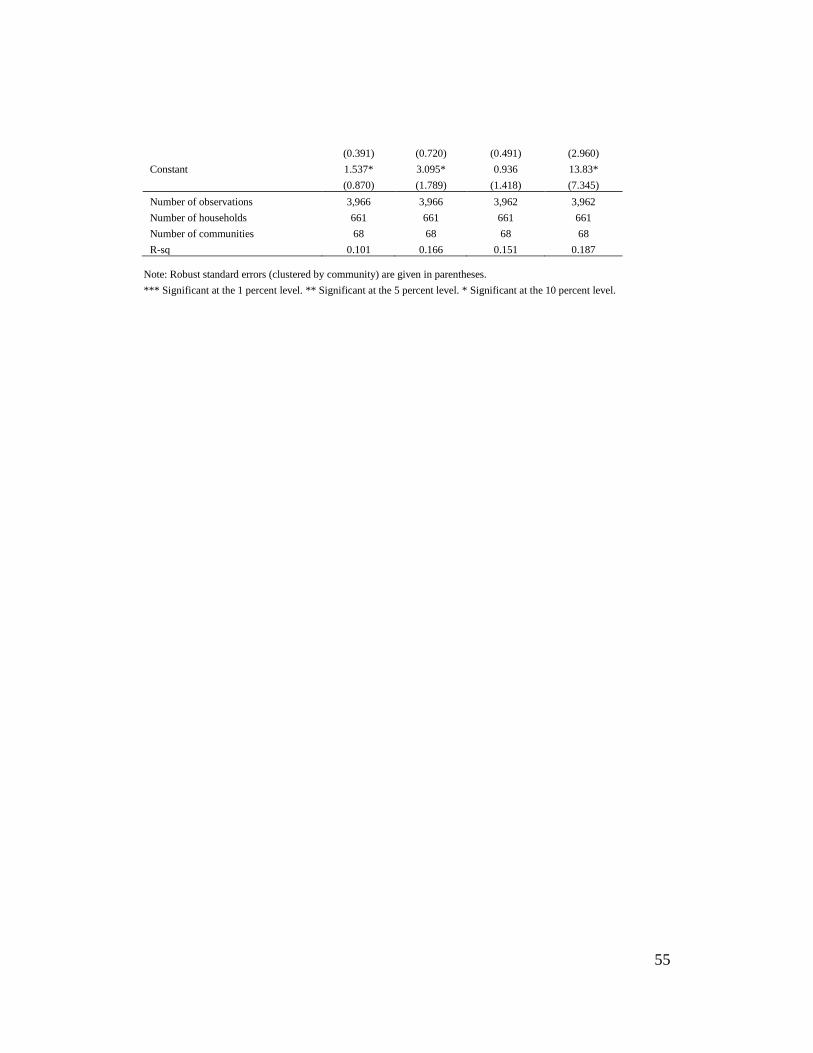
1{past use chem. fertilizers on maize} 0.489 1.509** 1.120** 6.712**

55

(0.391) (0.720) (0.491) (2.960)

Constant 1.537* 3.095* 0.936 13.83*

(0.870) (1.789) (1.418) (7.345)

Number of observations 3,966 3,966 3,962 3,962

Number of households 661 661 661 661

Number of communities 68 68 68 68

R-sq 0.101 0.166 0.151 0.187

Note: Robust standard errors (clustered by community) are given in parentheses.


56

TABLE 6. DETERMINANTS OF INPUT PURCHASE AMONG TREATMENT HOUSEHOLDS: COMMUNITY-FIXED EFFECT

REGRESSION

Dependent variables

Control variables

Hybrid seed

(kg)

Base

fertilizer (kg)

Top-dressing

fertilizer (kg)

Aggregate

quantity index

(1,000 Ush)

(1) (2) (3) (4)

Yield gain of experimental plot (kg) 0.002 0.012** 0.008** 0.045**

(0.002) (0.005) (0.003) (0.022)

Price –1.433*** –4.664*** –2.640*** –18.82***

(0.339) (0.745) (0.557) (2.689)

1{Credit sales} 1.690*** 17.00*** 5.858* 50.38***

(0.488) (5.161) (2.934) (12.98)

Down-payment rate * 1{Credit sales} –1.71 –31.74** –4.609 –79.77**

(1.441) (15.27) (6.753) (35.11)

Interest rate * 1{Credit sales} 0.223 –18.1 –7.91 –47.61

(3.981) (18.60) (15.85) (64.74)

Household size 0.0987* 0.466*** 0.258*** 1.725***

(0.058) (0.135) (0.095) (0.579)

Dependency rate –0.034 0.0197 0.256 0.356

(0.207) (0.397) (0.213) (1.504)

1{Female-headed HH} –0.193 –0.467 –0.784 –2.952

(0.370) (0.932) (0.824) (3.764)

Head’s age –0.0007 –0.013 –0.014 –0.048

(0.012) (0.030) (0.025) (0.116)

Head’s ears of schooling 0.094 0.181 –0.115 0.526

(0.066) (0.153) (0.072) (0.479)

Amount of land owned (ha) –0.004 –0.070*** 0.039** –0.091

(0.006) (0.013) (0.016) (0.059)

Asset holdings (millions of Ush) 0.089*** 0.200*** 0.009 0.756***

(0.026) (0.051) (0.025) (0.203)

1{past use of maize Hybrid seed} 1.582** 1.585 0.59 9.812*

(0.773) (1.104) (1.020) (5.442)

1{past use chem. fertilizers on maize} –0.362 0.231 0.331 –0.258

(0.446) (0.875) (0.667) (3.824)

Constant 1.767* 0.267 1.146 8.364

(0.909) (2.589) (1.894) (8.985)



R-sq 0.109 0.226 0.194 0.233



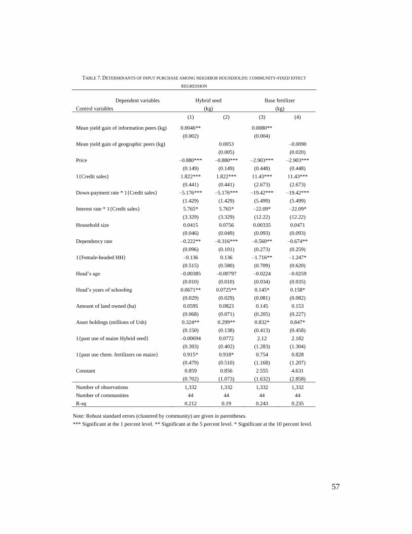
57

TABLE 7. DETERMINANTS OF INPUT PURCHASE AMONG NEIGHBOR HOUSEHOLDS: COMMUNITY-FIXED EFFECT

REGRESSION

Dependent variables

Control variables

Hybrid seed

(kg)

Base fertilizer

(kg)

(1) (2) (3) (4)

Mean yield gain of information peers (kg) 0.0046** 0.0080**

(0.002) (0.004)

Mean yield gain of geographic peers (kg) 0.0053 –0.0090

(0.005) (0.020)

Price –0.880*** –0.880*** –2.903*** –2.903***

(0.149) (0.149) (0.448) (0.448)

1{Credit sales} 1.822*** 1.822*** 11.43*** 11.43***

(0.441) (0.441) (2.673) (2.673)

Down-payment rate * 1{Credit sales} –5.176*** –5.176*** –19.42*** –19.42***

(1.429) (1.429) (5.499) (5.499)

Interest rate * 1{Credit sales} 5.765* 5.765* –22.09* –22.09*

(3.329) (3.329) (12.22) (12.22)

Household size 0.0415 0.0756 0.00335 0.0471

(0.046) (0.049) (0.093) (0.093)

Dependency rate –0.222** –0.316*** –0.560** –0.674**

(0.096) (0.101) (0.273) (0.259)

1{Female-headed HH} –0.136 0.136 –1.716** –1.247*

(0.515) (0.580) (0.709) (0.620)

Head’s age –0.00385 –0.00797 –0.0224 –0.0259

(0.010) (0.010) (0.034) (0.035)

Head’s ears of schooling 0.0671** 0.0725** 0.145* 0.158*

(0.029) (0.029) (0.081) (0.082)

Amount of land owned (ha) 0.0595 0.0823 0.145 0.153

(0.068) (0.071) (0.205) (0.227)

Asset holdings (millions of Ush) 0.324** 0.299** 0.832* 0.847*

(0.150) (0.138) (0.413) (0.458)

1{past use of maize Hybrid seed} –0.00694 0.0772 2.12 2.182

(0.393) (0.402) (1.283) (1.304)

1{past use chem. fertilizers on maize} 0.915* 0.918* 0.754 0.828

(0.479) (0.510) (1.168) (1.207)

Constant 0.859 0.856 2.555 4.631

(0.702) (1.073) (1.632) (2.858)



R-sq 0.212 0.19 0.243 0.235



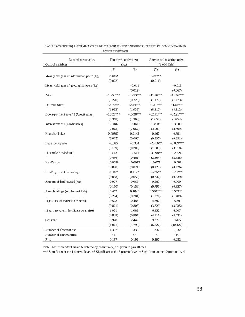
58

TABLE 7 (CONTINUED). DETERMINANTS OF INPUT PURCHASE AMONG NEIGHBOR HOUSEHOLDS: COMMUNITY-FIXED

EFFECT REGRESSION

Dependent variables

Control variables


(kg)

Aggregated quantity index

(1,000 Ush)

(5) (6) (7) (8)

Mean yield gain of information peers (kg) 0.0022 0.037**

(0.002) (0.016)

Mean yield gain of geographic peers (kg) –0.011 –0.018

(0.012) (0.067)

Price –1.253*** –1.253*** –11.16*** –11.16***

(0.220) (0.220) (1.173) (1.173)

1{Credit sales} 7.514*** 7.514*** 41.61*** 41.61***

(1.932) (1.932) (8.812) (8.812)

Down-payment rate * 1{Credit sales} –15.28*** –15.28*** –82.91*** –82.91***

(4.368) (4.368) (19.54) (19.54)

Interest rate * 1{Credit sales} –8.046 –8.046 –33.03 –33.03

(7.962) (7.962) (39.09) (39.09)

Household size 0.00893 0.0142 0.167 0.391

(0.065) (0.063) (0.297) (0.291)

Dependency rate –0.325 –0.334 –2.416** –3.009***

(0.199) (0.209) (1.003) (0.918)

1{Female-headed HH} –0.63 –0.501 –4.998** –2.824

(0.496) (0.462) (2.304) (2.388)

Head’s age –0.0080 –0.0073 –0.075 –0.096

(0.020) (0.021) (0.122) (0.126)

Head’s ears of schooling 0.109* 0.114* 0.725** 0.782**

(0.058) (0.059) (0.337) (0.339)

Amount of land owned (ha) 0.077 0.065 0.683 0.760

(0.150) (0.156) (0.790) (0.857)

Asset holdings (millions of Ush) 0.453 0.484* 3.518*** 3.509**

(0.274) (0.281) (1.270) (1.409)

1{past use of maize HYV seed} 0.503 0.483 4.892 5.29

(0.801) (0.807) (3.829) (3.935)

1{past use chem. fertilizers on maize} 1.031 1.083 6.352 6.607

(0.838) (0.804) (4.316) (4.531)

Constant 0.928 2.442 9.777 16.65

(1.001) (1.796) (6.327) (10.420)



R-sq 0.197 0.199 0.297 0.282



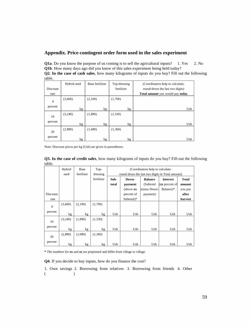
59

Appendix. Price-contingent order form used in the sales experiment

Q1a. Do you know the purpose of us coming is to sell the agricultural inputs? 1. Yes 2. No

Q1b. How many days ago did you know of this sales experiment being held today?

Q2. In the case of cash sales, how many kilograms of inputs do you buy? Fill out the following

table.

Discount

rate

Hybrid seed Base fertilizer Top-dressing

fertilizer

(Coordinators help to calculate;

round-down the last two digits)

Total amount you would pay today

0

percent

(3,600)

kg

(2,100)

kg

(1,700)

kg Ush

10

percent

(3,240)

kg

(1,890)

kg

(1,530)

kg Ush

20

percent

(2,880)

kg

(1,680)

kg

(1,360)

kg Ush

Note: Discount prices per kg (Ush) are given in parentheses.

Q3. In the case of credit sales, how many kilograms of inputs do you buy? Fill-out the following

table.

Hybrid

seed

Base

fertilizer

Top-

dressing

fertilizer

(Coordinators help to calculate;

round down the last two digits in Total amount)

Discount

rate

Sub-

total

Down-

payment

(above xx

percent of

Subtotal)*

Balance

(Subtotal

minus Down-

payment)

Interest

(zz percent of

Balance)*

Total

amount

you pay

after

harvest

0

percent

(3,600)

kg

(2,100)

kg

(1,700)

kg Ush Ush Ush Ush Ush

10

percent

(3,240)

kg

(1,890)

kg

(1,530)


20

percent

(2,880)

kg

(1,680)

kg

(1,360)


* The numbers for xx and zz are preprinted and differ from village to village.

Q4. If you decide to buy inputs, how do you finance the cost?

1. Own savings 2. Borrowing from relatives 3. Borrowing from friends 4. Other

( )

Documents

Technology Adoption and Dissemination in Agriculture ... · 1 Technology Adoption and Dissemination in Agriculture: Evidence from Sequential Intervention in Maize Production in Uganda