Embed Size (px)
Citation preview
Risk Aversion and Adoption of Conservation Agriculture Practices in Eastern Uganda
Barry Weixler-Landis
Thesis submitted to the faculty of the Virginia Polytechnic Institute and State
University in partial fulfillment of the requirements for the degree of
Master of
Science In
Agricultural and Applied Economics
George W. Norton, Committee
Chair Darrell J. Bosch
Jeffrey R. Alwang
April 9, 2014
Blacksburg, VA
Keywords: Partial Risk Aversion, Ordered Probit, Ordered Lottery Selection
Copyright Barry Weixler-Landis 2014

Risk Aversion and Adoption of Conservation Agriculture Practices in Eastern Uganda
Barry Weixler-Landis
ABSTRACT
Many poor farmers, especially in Africa, have not adopted recent farming innovations to
improve their yields. One theory is that poor farmers are risk averse and therefore do not invest
in high risk high return innovations and that risk averse farmers will only adopt larger
innovations if they experience success with small ones. Risk preferences were measured in two
districts in Uganda (Tororo and Kapchorwa) where adoption of agricultural innovations has been
slow, and where a program is underway to encourage use of conservation agriculture practices
(CAPs) to reduce soil erosion and sequester carbon. An ordered lottery selection was used to
measure risk preferences and an ordered probit model was estimated. Thirty five percent of a
random sample of 200 farmers in Tororo (and fifty three percent of 200 farmers in Kapchorwa)
made lottery choices that implied severe or extreme risk aversion. However there was no
indication that risk preferences correlate with willingness to adopt new technologies (such as
CAPs). Neither wealth nor previous success with technology adoption were found to correlate
with farmers’ risk preferences.
iii
Acknowledgments
I would like to express my gratitude first to Dr. George Norton who was very supportive and
knowledgeable; I would also like to thank Dr. Darrell Bosch and Dr. Jeff Alwang for their input.
A special thanks to the staff at Appropriate Technologies Uganda and the enumerators without
who’s help I would not have collected such good data in Uganda. Thanks also to Kate Vaiknoras
who worked with me to compile our surveys making it possible to reach more farmers in our
limited resources and time in Uganda. This project was supported by Sustainable Agriculture
and Natural Resource Management Innovation Lab.
iv
Table of Contents
Chapter 1: Introduction .................................................................................................................. 1
Objective ......................................................................................................................................... 3
Hypotheses ..................................................................................................................................... 3
Chapter 2: Background ................................................................................................................... 4
Chapter 3: Conceptual Framework .............................................................................................. 9
Risk Measures .............................................................................................................................. 10
Hypothetical vs. Paid Lottery ....................................................................................................... 14
Chapter 4: Methods ....................................................................................................................... 18
Data Collection ............................................................................................................................. 20
Risk Aversion Measurement ........................................................................................................ 21
Validation of Respondents’ Comprehension ............................................................................... 24
Conceptual Model ........................................................................................................................ 26
Chapter 5: Empirical Model ........................................................................................................ 28
Summary of Descriptive Statistics ............................................................................................... 29
Models .......................................................................................................................................... 32
Chapter 6: Results ......................................................................................................................... 34
Estimation Results ........................................................................................................................ 35
Discussion ..................................................................................................................................... 38
Conclusions .................................................................................................................................. 40
References ....................................................................................................................................... 43
Appendix A: Safety First .............................................................................................................. 45
Appendix B: Uganda Survey ....................................................................................................... 52
v
List of Tables
Table 1: Tororo Lottery Risk Measures ...................................................................................... 12
Table 2: Kapchorwa Lottery Risk Measures .............................................................................. 12
Table 3: Variables in the Model ................................................................................................... 29
Table 4: Summary of Descriptive Statistics for Tororo ............................................................ 32
Table 5: Summary of Descriptive Statistics for Kapchorwa ..................................................... 32
Table 6: Tororo Ordered Probit Coefficient Estimates ............................................................. 35
Table 7: Kapchorwa Ordered Probit Coefficient Estimates ..................................................... 36
Table 8: Tororo Marginal Effects ................................................................................................ 37
Table 9: Kapchorwa Marginal Effects ........................................................................................ 37
Table A1: Tororo Lottery Game 1 and 2 side by side ............................................................ 46
Table A2: Kapchorwa Lottery Game 1 and 2 side by side .................................................... 47

vi
List of Figures
Figure 1: Tororo Lottery Risk Frontier ...................................................................................... 12
Figure 2: Kapchorwa Lottery Risk Frontier .............................................................................. 12
Figure 3: Lottery Choice Practice Game .................................................................................... 22
Figure 4: Lotteries Chosen Tororo .............................................................................................. 34
Figure 5: Lotteries Chosen Kapchorwa .................................................................................... 34
Figure A1: Ccombination of lotteries chosen from both games in Tororo ............................ 49
Figure A2: Combination of lotteries chosen from both games in Kapchorwa ..................... 49
Figure B1: Ordered Lottery Selection used to elicit risk preference in Tororo .................... 58
Figure B2: Ordered Lottery Selection used to test safety-first in Tororo .............................. 59
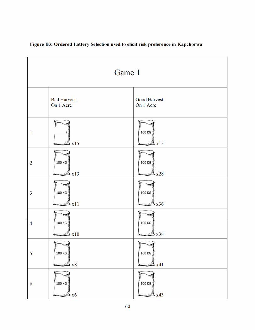
Figure B3: Ordered Lottery Selection used to elicit risk preference in Kapchorwa ............. 60
Figure B4: Ordered Lottery Selection used to test safety-first in Tororo ............................... 61
1
Chapter 1: Introduction
The Green Revolution increased agricultural productivity in numerous countries, especially in
Asia and Latin America. However, not all countries were able to capitalize on the improved
farming technologies. Uganda for example still has 66 percent of its labor force working on
farms and yet remains a net food importer.1 One theory as to why countries like Uganda have
not capitalized on higher yield technologies is that the poor are too risk averse to invest in high-
risk, high-return investments. Poor farmers continue to farm with their old proven techniques
and do not capitalize on farming innovations in order to avoid production risk.
Conservation agriculture practices (CAPs) may help increase food production, decrease
labor needs, and provide environmental benefits such as soil retention and carbon sequestration.
Practices such as minimum tillage, cover crops, and beneficial crop rotations have the potential
to increase soil fertility and slow soil erosion. These CAPs also sequester carbon by increasing
the organic matter in the soil. Many farming techniques can deplete the soil’s quality over years
of use, lowering future yields. The development and spread of CAPs, especially in developed
countries and on larger farms in developing nations, have demonstrated their potential benefits in
recent years.2
Unfortunately, adoption of CAPs has been slow among limited-resource farms in
developing countries. These farms are the majority of farms in the world. The importance of
improving agricultural productivity to raise incomes of low-income farmers, and of sequestering
carbon to help mitigate climate change has created pressures to design and disseminate CAPs for
small farms. A conservation agriculture program called the Sustainable Agriculture and Natural
Resource Management Innovation Lab (SANREM IL) was formed with a goal to design CAPs
1 Most recent year available:2010 from www.data.un.org/CountryProfile.aspx?crName=Uganda (1/2014) 2 www.icarda.org

2
that will increase or at least maintain soil productivity on small farms in developing counties,
improve food security for the farmers, and provide global environmental services such as
sequestering carbon. Uganda is one of the countries in which the SANREM IL research is
focused.3 The research is aimed at increasing yields reducing labor and other input costs, while
improving the soil quality.
Even if SANREM IL research develops a farming system that meets these goals, there is
no guarantee that Ugandan farmers will adopt the system. The CAPs techniques in Uganda are
tailored to overcome barriers to adoption such as high investment and labor costs. However, fear
of an unknown technique may cause people not to adopt the CAPs. Although CAPs may
increase yields in the future, they seldom result in dramatic first-year effects on yields or profits.
Only after a few years of nitrogen-fixing rotations and leaving cover crops on the field will larger
yield benefits begin to accrue. Therefore, the incentives to adopt a completely new farming
system may not be immediate enough to overcome people’s aversion to trying something new.
Partial adoption of the CAPs will most likely not benefit the farmer since it is the
interaction of the techniques that yields the greatest benefit. Therefore CAPs require an adopter
to learn an entirely new system with many unknowns. It might be easy to convince a risk-neutral
farmer to give it a try, but a risk-averse farmer may require more convincing to change farming
techniques they learned from their fathers and mothers. Risk aversion may be a substantial
barrier to the adoption of CAPs even when other barriers to adoption are addressed. Therefore, it
is important to assess the degree of risk aversion of Ugandan farmers in the area where the
SANREM IL project is focused.
3 http://www.oired.vt.edu/sanremcrsp/ (03/2013).

3
Objective The objective of this thesis is to assess the degree of risk aversion of farmers in eastern Uganda.
Hypotheses
1. Increased wealth decreases risk aversion of farmers in eastern Uganda
2. Previous success with new technologies (i.e. improved seed varieties or
fertilizers) decreases the farmers’ risk aversion, and failures with new
technologies increase risk aversion
Previous research on measuring risk aversion is reviewed in Chapter 2. Chapter 3 discusses the
conceptual framework for measuring risk aversion. Chapter 4 presents the methods used for
collecting the data. Chapter 5 gives the empirical model and presents the descriptive statistics.
In Chapter 6 the results are discussed and conclusions given.

4
Chapter 2: Background Are subsistence farmers risk averse? In the 1960s there was debate in the field of economic
development whether or not subsistence farmers optimized by equating their marginal value
product across all inputs. Shultz (1964) argued “there are comparatively few significant
inefficiencies in the allocation of the factors of productions in traditional agriculture” (p.37).
One of Shultz’s key arguments came from W. David Hopper who collected detailed production
data in Senapur India. Hopper (1965) estimated marginal values of some inputs of production
(land, bullock time, labor, and irrigation water) across four different crops (barley, wheat, pea,
and gram). Hopper and Shultz both agreed that these subsistence farmers were equating
marginal values of their farming inputs across their crops.
Michael Lipton (1968) on the other side of the debate pointed out that Hopper did not
include dung, a key input in his marginal value estimates. Lipton goes on to argue that when the
model is expanded to include dong reallocation of inputs in Senapur India could increase
production ten percent (Lipton, 1968). Hence, while farmers may be rational, they are not
simply profit maximizers. Lipton argued that farmers were not optimizing their marginal value
product of inputs because they were risk averse and made decisions based on a safety-first
algorithm. While researching in India, Lipton witnessed the volatility of weather, especially
rainfall, and hypothesized that people cannot adequately guess the probability of high or low
rainfall. He argued they have learned which techniques will protect them from the greatest
catastrophe, and rather than try to optimize their profits, they use the technique that will protect
them from the failures that will cause irreparable harm. Lipton assumed people living close to
starvation and without explicit safety nets will be forced to do things like sell their land and other
valuable assets or hire themselves out as indentured servants if a catastrophe strikes. Lipton
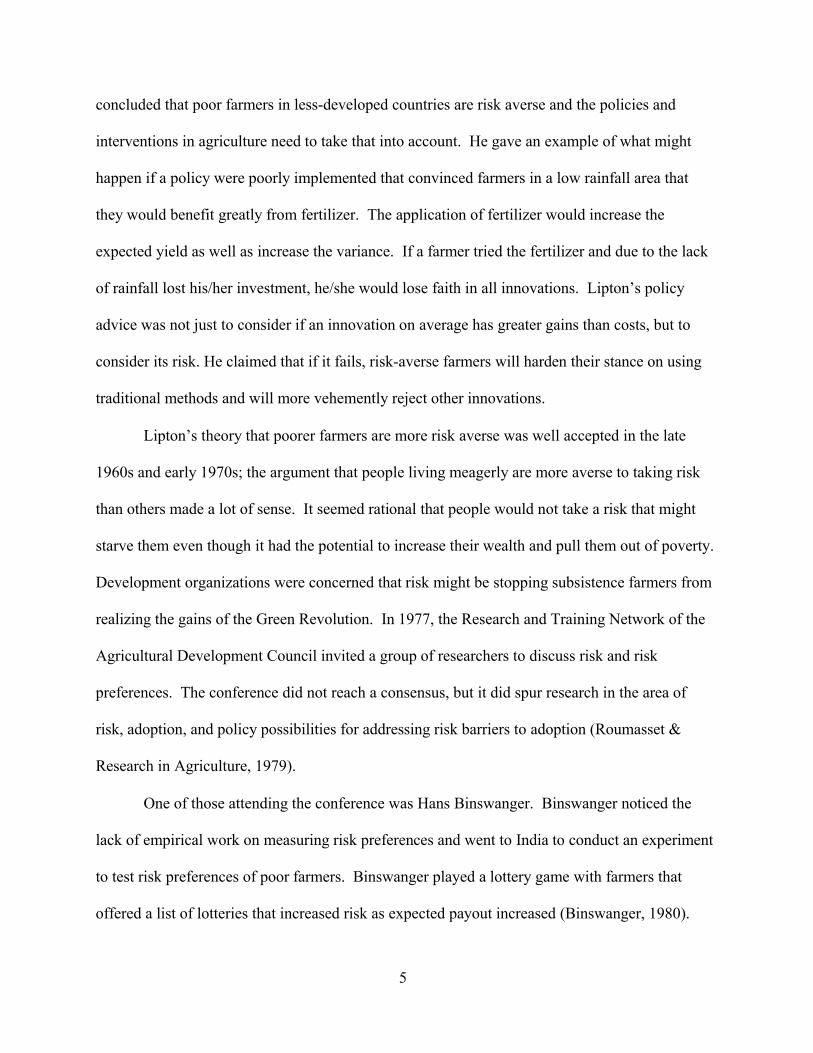
5
concluded that poor farmers in less-developed countries are risk averse and the policies and
interventions in agriculture need to take that into account. He gave an example of what might
happen if a policy were poorly implemented that convinced farmers in a low rainfall area that
they would benefit greatly from fertilizer. The application of fertilizer would increase the
expected yield as well as increase the variance. If a farmer tried the fertilizer and due to the lack
of rainfall lost his/her investment, he/she would lose faith in all innovations. Lipton’s policy
advice was not just to consider if an innovation on average has greater gains than costs, but to
consider its risk. He claimed that if it fails, risk-averse farmers will harden their stance on using
traditional methods and will more vehemently reject other innovations.
Lipton’s theory that poorer farmers are more risk averse was well accepted in the late
1960s and early 1970s; the argument that people living meagerly are more averse to taking risk
than others made a lot of sense. It seemed rational that people would not take a risk that might
starve them even though it had the potential to increase their wealth and pull them out of poverty.
Development organizations were concerned that risk might be stopping subsistence farmers from
realizing the gains of the Green Revolution. In 1977, the Research and Training Network of the
Agricultural Development Council invited a group of researchers to discuss risk and risk
preferences. The conference did not reach a consensus, but it did spur research in the area of
risk, adoption, and policy possibilities for addressing risk barriers to adoption (Roumasset &
Research in Agriculture, 1979).
One of those attending the conference was Hans Binswanger. Binswanger noticed the
lack of empirical work on measuring risk preferences and went to India to conduct an experiment
to test risk preferences of poor farmers. Binswanger played a lottery game with farmers that
offered a list of lotteries that increased risk as expected payout increased (Binswanger, 1980).
6
He reported that wealth was not an indicator of a person’s risk aversion. Binswanger concluded
that risk aversion is not what keeps poor farmers from adopting new technologies and pointed to
other constraints such as lack of credit, market access, and extension information. Binswanger’s
use of an experiment to measure risk preferences allowed people to make risky decisions without
being constrained by a lack of liquidity, credit, labor, and other market failures that subsistence
farmers often face in less-developed countries. When risk preferences are measured from
observing people’s daily choices, these constraints confound the data. It is hard to say if a
person does not choose a particular new farming technique because of risk preference or because
of a limiting constraint like lack of credit or information.
Binswanger offered eight lotteries ranging from risk neutral to severely risk averse for the
respondents to choose from. Binswanger wanted to know if there was a demographic or
observable situation that caused farmers to be more risk averse than their neighbors. He did not
find a significant attribute of poorer farmers that correlated with greater risk aversion. The
theory that those close to a subsistence level are more risk averse was not supported by his
empirical work. In his seminal paper, Binswanger (1980) concluded “it is not the innate or
acquired taste that hold the poor back but external constraints” (p.406).
Since Binswanger’s time, a few economists have replicated his research with similar
studies in less-developed countries; some have found similar results, some have found that
poorer farmers are more risk averse than wealthier farmers. Binswanger (1980), Mosley &
Verschoor (2005), and Cook (2011) have not found a significant correlation between risk
preferences and wealth. However, Wik et al. (2004) and Yesuf & Bluffstone (2004) found a
significant negative correlation between risk aversion and wealth, concluding that poorer farmers
are more risk averse.
7
The problem with risk aversion and wealth being negatively correlated is that poor risk-
averse farmers might not invest in innovations that yield higher returns due to higher risk. Risk
aversion might create a vicious cycle of poverty in which people stay in poverty due to their
choices to avoid high-risk, high-return investments. Mosley & Verschoor (2005) diagramed the
vicious cycle of poverty simply; if poverty leads to increased risk aversion and risk-averse
people invest in low return investments then their asset levels remain low, trapping them in
poverty. Like Binswanger, they found no significant evidence that the poorer are more risk
averse than others, thus the vicious cycle of poverty should not trap them. If poorer farmers are
not risk averse, they should be willing to make high risk/return investments. On average taking
higher risk and getting higher return will allow poorer farmers to accumulate assets for
consumption smoothing and increase their food security, ultimately escaping poverty. Also like
Binswanger, Mosley and Verschoor concluded that risk aversion is not innate in the poor but
market constraints like lack of insurance and credit are the problem.
Yesuf & Bluffstone (2004) using data from the highlands of Ethiopia found that one to
two thirds of the respondents were severely or extremely risk averse. They also found that small
amounts of accumulated wealth reduced people’s risk aversion. Their result suggests that the
poor are caught in a vicious cycle of poverty, and that a little wealth accumulation may decrease
their risk aversion, enabling them to make high risk/return investments to escape poverty. This
finding is in stark contrast to Binswanger, Mosley and Verschoor. Yesuf and Bluffstone also
found that previous success reduced a respondent’s risk aversion. These findings suggest that
escaping poverty may require or at least be greatly helped by intervention in risk mitigation.
They concluded that poor farmers are path dependent since their risk aversion will decrease with
small successes. Yesuf & Bluffstone (2004) concluded with a hopeful policy suggestion: “the

8
possibility of path dependence due to prior success and changes in wealth indicates that rural
development efforts do well to assure initial successes that can serve to demonstrate the
conditions under which investments are viable” (p.1034)
The past decades governments and non-governmental organizations have attempted to
remove some of the constraints facing farmers by setting up micro-credit organizations and
combining agricultural research with extension. Programs such as SANREM IL and
organizations such as IFPRI have strategically focused their research on key agricultural
products to have the maximum impact on food security. However, relatively little has been done
to assess the risk attitudes of farmers in many of the poorest developing countries. If risk
aversion is not a barrier to adoption, then no special attention needs to be devoted to it and
research to cope with actual risk should get priority. However, if Lipton’s argument is valid,
policies and extension programs need to consider the risk attitudes of the stakeholders as well as
the risk portfolio of their innovations. This paper adds to the body of knowledge by measuring
risk aversion in two rural districts in eastern Uganda to see if risk aversion is a barrier to
adopting CAPs.
9
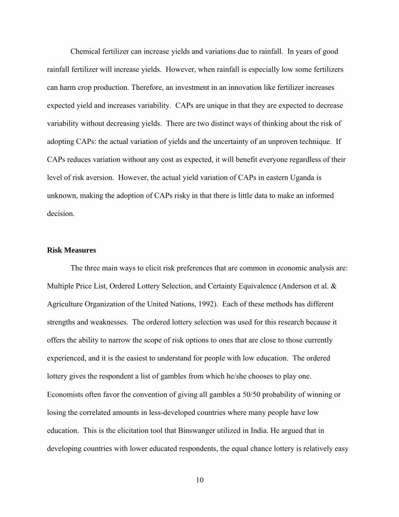
Chapter 3: Conceptual Framework People’s attitudes toward risk are relative to the options available to them. People could be
averse to risk at all levels but must still choose a portfolio of options that has a fair amount of
risk in it because they do not have the option to sustain their life with a risk-free portfolio. Since
everyone has to make decisions in a world of risky options, they will make those decisions based
on the knowledge, experience, and options available to them.
When considering the risk of adopting a new farming technique like the CAPs being
studied by SANMREM IL a farmer cannot simply look at the expected yields and variations of
harvests because it has not been exhibited for years by all his/her neighbors. The first adopters
of a new technique have to make their risk decisions with a lot of uncertainty about the actual
risk portfolio of the technique. How people make risky decisions under uncertainty is beyond
the scope of this paper. This paper follows the convention of the authors eliciting risk
preferences cited earlier in this paper by offering an experiment were respondents choose an
option from differing risks and payouts.
There is no direct and tractable way to pin-point what level of risk aversion is an ultimate
barrier to adoption; it would be nice to know at what precise risk measure is a barrier to
adoption. In the absence of this level of research many economists have used ranges to stratify
people’s risk aversion into different classifications (Binswanger, 1980; Miyata, 2003; Wik,
Kebede, Bergland, & Holden, 2004; Yesuf & Bluffstone, 2009). These researchers have
assumed those with greater measured risk aversion will be slower to take the risk of adopting a
new farming technique and those with lower risk aversion will be quicker to take the risk of a
new farming technique. Similarly, the adoption of CAPs can be estimated by hypothesizing that
farmers in certain risk aversion ranges are too risk averse to adopt.
10
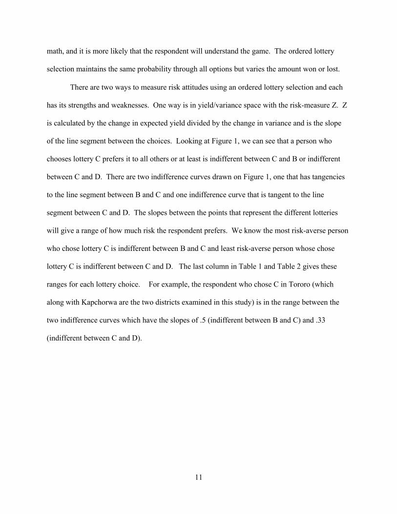
Chemical fertilizer can increase yields and variations due to rainfall. In years of good
rainfall fertilizer will increase yields. However, when rainfall is especially low some fertilizers
can harm crop production. Therefore, an investment in an innovation like fertilizer increases
expected yield and increases variability. CAPs are unique in that they are expected to decrease
variability without decreasing yields. There are two distinct ways of thinking about the risk of
adopting CAPs: the actual variation of yields and the uncertainty of an unproven technique. If
CAPs reduces variation without any cost as expected, it will benefit everyone regardless of their
level of risk aversion. However, the actual yield variation of CAPs in eastern Uganda is
unknown, making the adoption of CAPs risky in that there is little data to make an informed
decision.
Risk Measures
The three main ways to elicit risk preferences that are common in economic analysis are:
Multiple Price List, Ordered Lottery Selection, and Certainty Equivalence (Anderson et al. &
Agriculture Organization of the United Nations, 1992). Each of these methods has different
strengths and weaknesses. The ordered lottery selection was used for this research because it
offers the ability to narrow the scope of risk options to ones that are close to those currently
experienced, and it is the easiest to understand for people with low education. The ordered
lottery gives the respondent a list of gambles from which he/she chooses to play one.
Economists often favor the convention of giving all gambles a 50/50 probability of winning or
losing the correlated amounts in less-developed countries where many people have low
education. This is the elicitation tool that Binswanger utilized in India. He argued that in
developing countries with lower educated respondents, the equal chance lottery is relatively easy
11
math, and it is more likely that the respondent will understand the game. The ordered lottery
selection maintains the same probability through all options but varies the amount won or lost.
There are two ways to measure risk attitudes using an ordered lottery selection and each
has its strengths and weaknesses. One way is in yield/variance space with the risk-measure Z. Z
is calculated by the change in expected yield divided by the change in variance and is the slope
of the line segment between the choices. Looking at Figure 1, we can see that a person who
chooses lottery C prefers it to all others or at least is indifferent between C and B or indifferent
between C and D. There are two indifference curves drawn on Figure 1, one that has tangencies
to the line segment between B and C and one indifference curve that is tangent to the line
segment between C and D. The slopes between the points that represent the different lotteries
will give a range of how much risk the respondent prefers. We know the most risk-averse person
who chose lottery C is indifferent between B and C and least risk-averse person whose chose
lottery C is indifferent between C and D. The last column in Table 1 and Table 2 gives these
ranges for each lottery choice. For example, the respondent who chose C in Tororo (which
along with Kapchorwa are the two districts examined in this study) is in the range between the
two indifference curves which have the slopes of .5 (indifferent between B and C) and .33
(indifferent between C and D).

12
6.5
Tororo Units in 100Kg bags of maize
E D
F
06 C .14
.3 5.5 B
.5
5A
4.5
4
.6
0 1 2 3 4 5 6 7
Total Variance
Kapchorwa Units in 100Kg bags of maize
E25
23
21
FC
D
.33 .2 0
B .6
19
17 A
15
13 0
.73
5 10 Total Variance
15 20
Figure 1: Tororo Lottery Risk Frontier Figure 2: Kapchorwa Lottery Risk Frontier
Note: Lotteries A-F for Tororo and Kapchorwa plotted in yield/variance space to show the trade-off between the lottery options, two indifference curves are drawn to represent how an individual who chose lottery option C could be indifferent between B and C or C and D . See footnote 4 for information on units and the methods section for why yields are different in the two regions.
Table 1: Tororo Lottery Risk Measures
Lottery Option
Number of 100 Kg bags of maize, bad harvest
Number of 100 Kg bags of maize, good harvest
Risk Aversion Classification
r=risk coefficient
Z=∆
∆
A 4.5 4.5 Extreme ∞ to 6.244 1 to .6B 4 6.5 Severe 6.244 to 1.674 .6 to .5C 3.5 8 Intermediate 1.674 to .720 .5 to .33 D 3 9 Moderate .720 to .190 .33 to .14E 1.5 11 Slight to Neutral .190 to 0 .14 to 0F 0 12.5 Neutral to Negative 0 to -∞ 0 to -∞
Table 2: Kapchorwa Lottery Risk Measures
Lottery Option
Number of 100 Kg bags of maize, bad harvest
Number of 100 Kg bags of maize, good harvest
Risk Aversion Classification
r=risk coefficient
Z=∆
∆
A 15 15 Extreme ∞ to 5.649 1 to .73B 13 28 Severe 5.649 to 1.419 .73 to .6C 11 36 Intermediate 1.419 to .55 .6 to .33D 10 38 Moderate .55 to .274 .33 to .2E 8 41 Slight to Neutral .274 to 0 .2 to 0 F 6 43 Neutral to Negative 0 to -∞ 0 to -∞
Exp
ecte
d Y
ield
Exp
ecte
d Y
ield

13
0 ′
One strength of analyzing risk preferences in expected yield/variation space is the straight
forward way in which it can be analyzed. The slope of the line segments can be interpreted as
the ‘price’ in increased yield that a farmer needs to receive to take on more risk. When the
expected yield and variation of the new CAPs are known, they can be compared to the ‘price’
captured by Z. Taking current yields and variations into account, adoption rates could be
estimated using Z as a price to take on or discard risk. Since the respondent is seeing all six
lottery choices at once, and only those six, there is no precise or final exchange for mean yield
and variation. There are only the exchanges between the given choices, but the actual mean and
variance of CAPs should lie within the range of this risk-frontier. Mean/variance analysis makes
it possible to discuss the substitution rate of expected mean and variation.
The second way this ordered lottery selection was analyzed was with a Von Neumann-
Morgenstern risk coefficient in Expected Utility Theory (EUT). The advantage of EUT analysis
is the mathematical tractability of the risk measures, and the risk coefficient is unit free and
therefore can be compared to other studies based on different pay amounts and different
currencies. Arrow and Pratt derived risk coefficients from EUT that can reflect absolute risk
aversion and relative risk aversion (Pratt, 1964). Building on Pratt and Arrow, Menezes and
Hanson (1970) defined a third coefficient: partial risk aversion:
1) P(W,π =- ′′
0
0
where W0denotes initial wealth, is stochastic income, and ′ ′′ indicate the first and second derivative of the expected utility function.
Absolute risk aversion describes situations where income is fixed and the initial wealth is
variable. Relative risk aversion is a good measure for situations where income and initial wealth
change proportionately. When initial wealth is fixed and income varies, partial risk aversion is
14
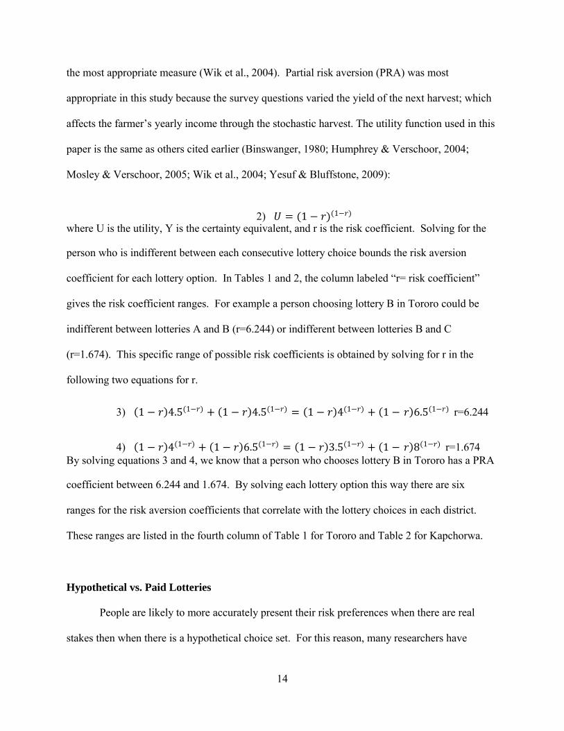
the most appropriate measure (Wik et al., 2004). Partial risk aversion (PRA) was most
appropriate in this study because the survey questions varied the yield of the next harvest; which
affects the farmer’s yearly income through the stochastic harvest. The utility function used in this
paper is the same as others cited earlier (Binswanger, 1980; Humphrey & Verschoor, 2004;
Mosley & Verschoor, 2005; Wik et al., 2004; Yesuf & Bluffstone, 2009):
2) 1 1
where U is the utility, Y is the certainty equivalent, and r is the risk coefficient. Solving for the person who is indifferent between each consecutive lottery choice bounds the risk aversion
coefficient for each lottery option. In Tables 1 and 2, the column labeled “r= risk coefficient”
gives the risk coefficient ranges. For example a person choosing lottery B in Tororo could be
indifferent between lotteries A and B (r=6.244) or indifferent between lotteries B and C
(r=1.674). This specific range of possible risk coefficients is obtained by solving for r in the
following two equations for r.
3) 1 4.5 1 1 4.5 1 1 4 1 1 6.5 1 r=6.244
4) 1 4 1 1 6.5 1 1 3.5 1 1 8 1 r=1.674 By solving equations 3 and 4, we know that a person who chooses lottery B in Tororo has a PRA
coefficient between 6.244 and 1.674. By solving each lottery option this way there are six
ranges for the risk aversion coefficients that correlate with the lottery choices in each district.
These ranges are listed in the fourth column of Table 1 for Tororo and Table 2 for Kapchorwa.
Hypothetical vs. Paid Lotteries
People are likely to more accurately present their risk preferences when there are real
stakes then when there is a hypothetical choice set. For this reason, many researchers have

15
played lotteries in which the respondents gamble real money. For ethical reasons when playing
lotteries in less-developed countries, most researchers only offer a win/win lottery with no
chance of the person losing their own money. The researcher using a lottery with real money has
little doubt that the respondent is answering the same question the researcher is asking on the
survey due to the power of the financial incentives. The ordered lottery selection with actual
payouts is a theoretically precise way of measuring risk preferences based on risk attitudes
toward money. However, the final analysis needs to translate this experiment into how farmers
make farming decisions under uncertainty in their fields.
When farmers make decisions in their fields, there may not be a direct correlation
between their stated degree of risk preference for monetary lottery games and their actions in real
life. When a farmer makes a choice from the list of lotteries, he/she does not have to consider
any of their real constraints, and the decision is based on how they think about risks and payoffs
at that time and place and at those amounts. The environment of a monetary gamble is different
from the field and the payout timelines are different too. Also since it is a win/win game, they
do not have to think about negative consequences of losing money from their normal budget.
When making a farming decision however, a farmer must think about the consequences of a
failed crop or very low yield. The farmer invests money in farming inputs which he/she hopes
will return a profit at harvest time. There is usually a family counting on the harvest for their
food and livelihood. This conundrum exists between precise experimental measurement of risk
aversion and the interpretation in the reality in which farmers make their farming decisions.
The weakness of the paid lottery becomes apparent when the findings are translated into
the farmers’ risk preferences for their livelihood across an entire growing season. A hypothetical
choice set based as closely as possible on farming reality combined with a well-constructed
16
script may even be a more accurate measure of farmers making their farming decisions than an
experiment with real money. This study used a hypothetical game anchored in the production
realities that farmers face. The game was anchored so that the respondents would view the
game as realistic and make their decisions to accept risk the same way they would at planting
time. In their decision process, they will include their loss aversion in that if they have a very
poor crop they will lose their investment and they may not be able to adequately feed their
family. A person who loses when gambling for real money in a win/win scenario, as has been
the custom in many risk-preference elicitation studies, does not have to worry about how it will
affect his/her budget since it is not part of their budget.
A hypothetical lottery is not part of their real budget either, but it can be anchored on
crop yields for an entire growing season. To payout real money at the level of a single harvest
would be too costly and paying people in produce a logistical nightmare. The unit used in this
hypothetical research is 100 kilogram bags of maize, which provided many benefits: it allowed
for the use of pictures since some respondents were illiterate, they sell their maize harvest in 100
kilogram bags, and maize is the most important crop.4
Since the benefits of CAPs are expected to be small incremental yield increases over a
few years, it is relevant to test the farmers’ preferences for risk at and around their current
combination of yields and variances. Anchoring the choice set around current yields not only
makes its hypothetical aspects more believable, it also means the measurement of risk aversion
may be relevant for a farmer making a decision about CAPs. Conservation agriculture is an
entirely new system of farming for most farmers, and it requires full commitment to accrue
benefits. Therefore, the perceived risk of the CAPs may be greater than the actual risk. This
4 The 100 KG bags are a standard size bag they fill with maize still on the cob; Ugandans do not weigh the bags or take the kernels off the cob.
17
research does not elicit farmers’ perception of the riskiness of CAPs, but the hypothetical lottery
spans a large enough range of believable crop harvest yields so as to catch a relevant range of
risk measures. Hypothetical bias is no small matter, but it can be minimized by how the choices
are presented; so much effort was given in training the enumerators to make sure the respondents
understood the survey and grounded the hypothetical choices in the respondents’ reality.
18
Chapter 4: Methods This study was administered in two districts in eastern Uganda: Tororo and Kapchorwa. These
districts were chosen because they are where SANREM IL is conducting its research and
demonstrations, both on-station and in the fields of participating farmers. SANREM IL is
researching CAPs based around maize because maize is the primary crop grown in eastern
Uganda.
It is assumed that adoption will start close to the fields of participating farmers and
spread out from there (Lamb, 2011). The two districts have very different climates, farming
techniques, and expected yields. Therefore, to properly anchor the lottery choice sets and control
for differences between the districts, different lotteries were designed for each district. It would
have been nice to design one lottery and administer it to 400 people, but to minimize
hypothetical bias and control for other differences Tororo respondents received a lottery set
based on their typical yields and Kapchorwa received a lottery set based on their typical yields.
These two sets provided the study with two separate groups of 200 respondents in each region.
Both districts are in eastern Uganda, but Tororo is lower, flatter, and more arid than
Kapchorwa. Tororo depends entirely on rainfall to water the fields and receives less rain than
Kapchorwa. Kaptchorwa not only receives more rain, but there are springs and streams that
provide some water when there are no rains. The soil quality in Kapchorwa is much better than
the sandy soil in Tororo.5 “Kapchorwa is one of the most productive districts in Uganda”.6 The
two districts have very different yields due to water availability, soil quality, and differences in
the use of fertilizer. Kapchorwa farmers use fertilizer and do not plant anything between their
rows of maize. Very few people in Tororo use fertilizer and most of them plant beans between
5 http://www.oired.vt.edu/sanremcrsp/professionals/research-activities/phase4/ltra10/ 6 A quoted from Grace Tino (director of Appropriate Technologies Uganda).
19
their rows of maize. The people interviewed in Kapchorwa reported that historically they also
planted beans between their rows of maize, but as the use of chemical fertilizer increased, they
found mono-cropping maize to be more profitable.
Due to their differences, CAPs are important to these two regions for different reasons.
Due to Kapchorwa’s steepness, soil erosion causes farmers to lose valuable land during heavy
rains. The minimal disturbance of the soil and leaving on cover crops of CAPs will help slow
erosion by keeping valuable topsoil in place. In Tororo, the soil is sandy and lacks nutrients to
produce high yields. By leaving the cover crop on the land, Tororo farmers can increase the
organic matter in their soil, which over time can increase yields. There may also be a benefit of
retained moisture in the soil since cover crops provide shade.
Because an accurate anchor is crucial in minimizing hypothetical bias, information about
the current mean and variation experienced in each region was obtained. Five experts/extension
agents and nine farmers were interviewed in Tororo and asked: “what is the average yield, the
yield for a typical bad harvest, and the yield for a typical good harvest? In Kapchorwa, three
experts/extension agents and nineteen farmers were interviewed. Within each district, people’s
answers were relatively homogenous, with the exception of two farmers in Tororo and three
farmers in Kapchorwa who indicated lower expected yields than the rest. Also, one farmer in
Tororo utilized advanced techniques compared to his neighbors and realized higher yields. That
farmer was running a test farm for SANREM IL and reported that the CAPs were working well.
He also used fertilizer along with the conservation farming techniques. The homogeneity of
farming techniques and the consistency of expected yield in each region made it feasible for the
lottery set to be anchored on a common experience. In Tororo, the average yield reported was 8-
10 bags, the bad harvest was complete crop loss, and the typical good harvest was 10-12 bags.

20
For Kapchorwa, respondents reported an average of 20 bags, a bad harvest was 10 bags, and a
good harvest was 40 bags.
Data Collection
The data for this paper were collected in June and July of 2013. The survey questionnaire was
designed to collect data for this study and another study that analyzed a choice model
experiment.7 To administer the survey, ten enumerators were recruited in Tororo and nine
enumerators in Kapchorwa. The farmers in these two regions spoke different languages and
needed different enumerators. One full day was spent in each district training the enumerators on
the survey. The first part of the survey included basic demographic questions; therefore,
significant time was spent during enumerator training to make sure everyone understood the risk-
preference elicitation game and the choice-model experiment.8
Two hundred farmers were randomly selected in each region by first randomly selecting
twenty villages from a list of all villages in each region. Ten people were then randomly selected
from each of the selected villages. The names of the villagers were obtained from the county
district office that had information from a 2007 census. Since the census was not recent, three
extra names were randomly selected from each village as a reserve in case some of the selected
farmers had died or moved away. The village randomization in Tororo was done by taking every
fourth village from an alphabetical list. The rest of the randomization was done with an Excel
random number generator. The surveys were administered by interview on the respondent’s
farm or wherever the respondent could be located. Researchers who invited farmers in to a
7 Kate Vaiknoras of Virginia Tech collected data for a choice experiment to ascertain the importance of environmental services to the Ugandan stakeholders. The survey form can be seen in the appendix 8 The choice-model experiment was the part of the survey relevant to Kate Vaiknoras.

21
central location i.e. (Binswanger, 1980; Cook, Chatterjee, Sur, & Whittington, 2013; Harrison,
Humphrey, & Verschoor, 2010; Mosley & Verschoor, 2005; Yesuf & Bluffstone, 2009) remove
farmers from their homes. This survey controlled for location influence by meeting most of the
respondents where they live and made farming decisions.
Risk Aversion Measurement
The respondents’ risk preferences were measured with a hypothetical game of six lottery choices
laid out on a concave risk frontier in the style of Binswanger. The first option was a completely
safe one with the same payout for winning or losing. The next four options had higher expected
yields and higher variances. Farmers ‘pay’ for the higher expected yield by taking on more risk.
The sixth and final choice increased the variance while keeping the expected yield equal to the
fifth choice; this option added the ‘cost’ of more risk without a higher payout. Tororo’s risk
frontier is shown in Figure 1 and Kapchorwa’s is shown in Figure 2. Each lottery option
consisted of a bad outcome of lower yield and a good outcome of higher yield with a 50/50
chance of good or bad. See Figure 3 for an example of the three lottery options used as a practice
game. If the first lottery (A) was chosen, it paid out 5 bags of maize if the person lost and 10
bags if the person won. If the second lottery (B) was chosen, it paid out 3 bags if the person lost
and 15 bags if the person won. Lottery choice C paid out nothing if the person lost and 20 bags
if the person won.
To make sure each respondent understood the equal chances of good or bad outcomes for
each lottery, a practice game was played first that consisted of three lottery options that covered
a large range of yields (see Figure 3). The respondent chose one of the lotteries and the
enumerator asked why they chose that lottery to make sure they understood they had an equal

23
A local game was used that everyone had played as a child and understood well. The
enumerator would show the person an object and hide it in a hand behind his/her back. The
enumerator would then show the respondent both closed fists and ask the person to pick a hand.
If the person picked the hand containing the object, they received a good harvest, but if the
person picked the empty hand they received a bad harvest. This game was very familiar to all
respondents because they had played it as children. The enumerator asked the respondent to talk
through the outcome. Playing the game once and discussing the outcome helped ground the
hypothetical aspect of the game in the farmer’s reality. To further ground the games before
moving on to the next two games, the enumerators asked the respondents to think of their budget,
family responsibilities, all the crops they grow, and how their decisions for planting maize on one
acre of land with the expected outcomes shown would affect their lives. Only the practice
game was played and discussed. For the actual risk elicitation game, the enumerators where
trained to only read through the options and record the person’s choose.
Farmers were told the actual risk elicitation game would not be played. They were told
to imagine the enumerator standing in the field at harvest time with two closed fists and whether
they won or lost the game at that time dictated the size of their harvest. This was done to place
the hypothetical game in the same time frame as farming decisions. Not finding out if they won
or lost immediately allowed them to make their decisions without being motivated by the
immediate emotion of playing the 50/50 game, and it helped control for hypothetical bias.
When the enumerator asked questions and interacted with the respondent during the
practice game, they were able to know if the person understood the task from the face-to-face
intimacy of the interview. Any coaching that might have gone on during the practice game was
disconnected from the actual risk-elicitation tool in two ways. First, the expected means and

24
variances of the practice game were different from the lottery options in the actual ordered
lottery list. That way, if the enumerator had coached them toward a certain lottery in the practice
game, that coaching would not easily transfer to a lottery in the actual elicitation tool. Second,
once the enumerators introduced the actual elicitation tool, they did not talk anymore about
grounding the lotteries in reality or how the game was played. They did that in the practice
game, but for the elicitation tool they only read the options to the farmer and recorded their
selections.
After the practice game was completed, each respondent made choices from two lottery
sets. The first choice set was a list of six lotteries (A-F) of bad and good yield expectations
designed to elicit a risk preference. The second choice was designed to test if Lipton’s theory
that subsistence farmers make decisions based on a safety-first algorithm has any validity and to
test for misunderstanding by including a risk-loving choice. The second game is discussed in
greater detail in the next section and appendix A (Safety-First).
Validation of Respondents’ Comprehension
Researchers want to know if the respondents understood the survey and answered the same
questions the researchers were asking. To determine whether or not respondents understood his
ordered lottery list, Binswanger (1980) included two inefficient choices. His two choices offered
the same expected payout as another lottery but with greater variance. Binswanger placed these
two options in the middle of the ordered lottery game so that the other lottery choices had
stochastic dominance over these inefficient choices. By doing this, Binswanger offered six
lottery choices on the risk frontier and two inefficient lotteries inside the risk frontier. If a
respondent did not understand the game and chose randomly, Binswanger’s verification method

25
would catch them two out of eight times or 25%, suggesting there could be more people
misunderstanding then ‘caught’ making a mistake. Binswanger (1980) had two hundred and
eighty-six people complete nine games each and found that 33% of them chose an inefficient
lottery at least once.
A multiple price list offers a list of choices between a safer and a riskier lottery. The risk
coefficient is measured where the person switches from the riskier to the safer lottery or vice
versa. Researchers using this method of eliciting risk preference can hypothesize that people
switching more than one time misunderstood the exercise or were inconsistent. Cook et al.
(2013) found that of the 404 respondents they surveyed, 238 or 59% of them made mistakes. It
is likely that Binswanger had as many people misunderstanding the exercise as Cook et al. did,
but the ordered lottery selection does not allow for mistakes as readily as a multiple price list.
Due to the difficulty in knowing whether a respondent understood the game based on the
data, this researcher primarily counted on the enumerator to ascertain if the person understood
the task during the practice game. The enumerators shared the same culture and language as the
respondents and had face-to-face interviews in which they tried to make sure the respondents
understood the task. Also a risk loving option was included in the second ordered lottery to
catch people making mistakes. This option (F*) gave lower expected yield and higher variance
than lotteries D and E.
One model is estimated in this paper in which the respondents who chose lottery F* in the
second game are left in and risk-loving behavior is allowed. A second model is estimated in
which respondents who chose lottery F* are removed and assumes Ugandan farmers are not risk
loving in terms of their yearly harvest but they made a mistake. Similar to Binswager’s
inefficient options, this risk loving option (F* in the second game) will only ‘catch’ one out of

26
six or 17% of the people making random choices. Therefore removing these respondents does
not guarantee that there are not mistakes in the data, but the reliability of the data is based on the
competency of the enumerator performing face-to-face interviews.
Conceptual Model
As stated earlier there are two assumptions about how risk aversion will effect adoption of CAPs.
We can assume those who are less risk averse will be quicker to try a new unproven farming
technique. This assumes that first adopters are generally not going to be the most risk-averse
people of a given population. Alternatively we can assume that since CAPs are expected to
decrease variability, farmers who are more risk averse will be equally quick to adopt them. The
author of this paper thinks that the unknown outcomes of CAPs are a greater barrier to adoption
than the unproven assumption that CAPs will decrease variation in eastern Uganda. Knowing
what observable characteristics correlate with decreased risk aversion will help estimate adoption
of CAPs. Also, once more is known about the CAPs, knowing what observable characteristics
are correlated with decreased risk aversion will aid extension agents by highlighting the farmers
more willing to try a new technique with the unique attributes of CAPs.
The primary characteristic of interest is the wealth of the farmers. As Lipton argued, the
poor lack tools to cope with loss and therefore will be more risk averse. If Lipton’s argument is
accurate it would be beneficial for extension agents to focus first on wealthier farmers since they
would be more likely to adopt a new technique. To test Yesuf and Bluffstone’s theory that the
poor are path dependent and need small guaranteed successes to gain the confidence to adopt
innovations on their own, this study asked respondents about previous successful and
unsuccessful innovations. If those with more previous successful innovations are less risk averse

27
and/or if those who felt their innovations have been unsuccessful are more risk averse, then this
study will support Yesuf and Bluffstone’s path dependency theory.
28
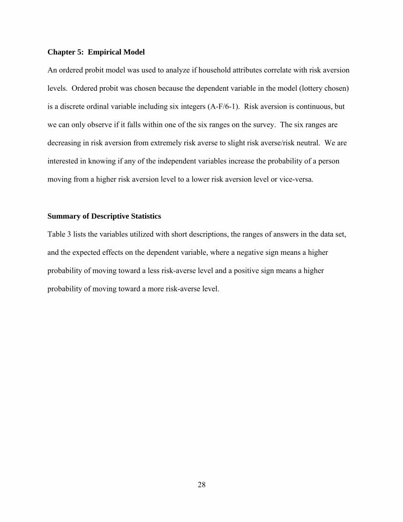
Chapter 5: Empirical Model An ordered probit model was used to analyze if household attributes correlate with risk aversion
levels. Ordered probit was chosen because the dependent variable in the model (lottery chosen)
is a discrete ordinal variable including six integers (A-F/6-1). Risk aversion is continuous, but
we can only observe if it falls within one of the six ranges on the survey. The six ranges are
decreasing in risk aversion from extremely risk averse to slight risk averse/risk neutral. We are
interested in knowing if any of the independent variables increase the probability of a person
moving from a higher risk aversion level to a lower risk aversion level or vice-versa.
Summary of Descriptive Statistics
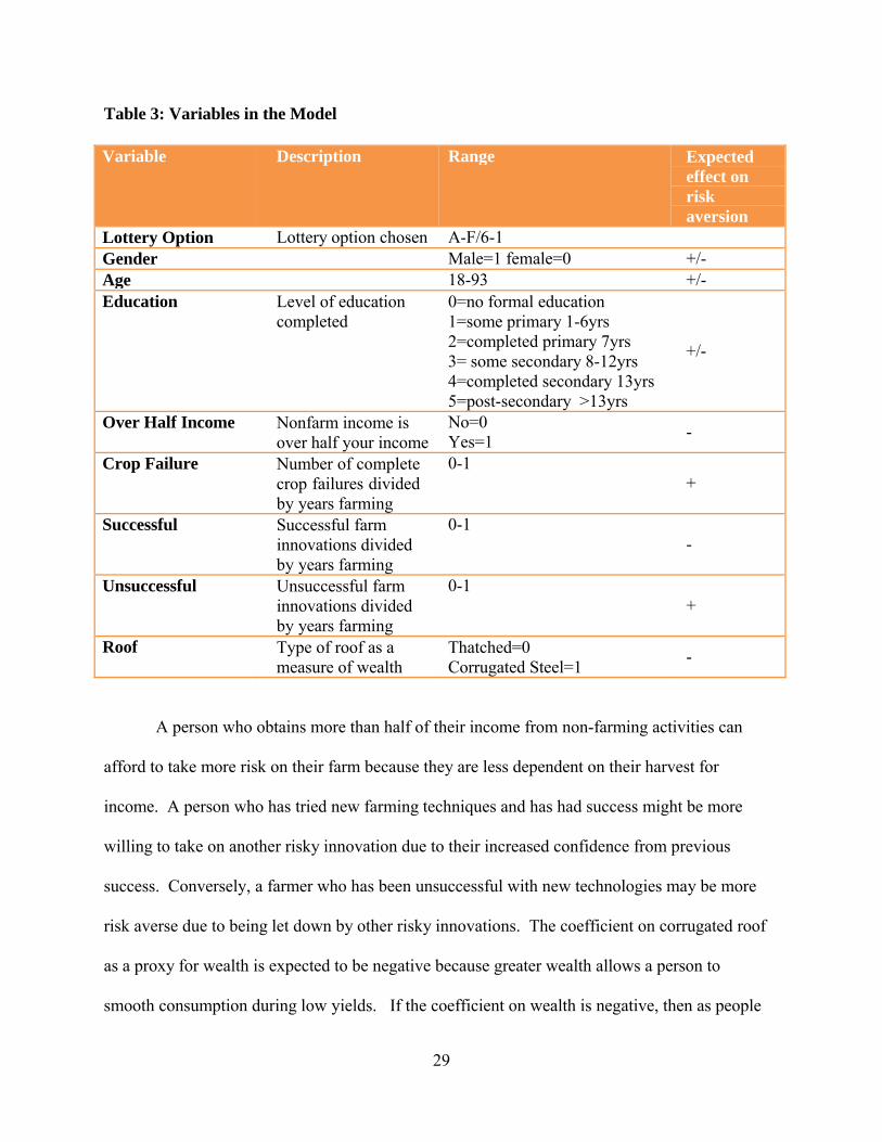
Table 3 lists the variables utilized with short descriptions, the ranges of answers in the data set,
and the expected effects on the dependent variable, where a negative sign means a higher
probability of moving toward a less risk-averse level and a positive sign means a higher
probability of moving toward a more risk-averse level.
29
Table 3: Variables in the Model
Variable Description Range Expected effect on risk aversion
Lottery Option Lottery option chosen A-F/6-1
Gender Male=1 female=0 +/- Age 18-93 +/- Education Level of education
completed 0=no formal education 1=some primary 1-6yrs 2=completed primary 7yrs 3= some secondary 8-12yrs 4=completed secondary 13yrs 5=post-secondary >13yrs
+/-
Over Half Income Nonfarm income is over half your income
No=0Yes=1
-
Crop Failure Number of complete crop failures divided by years farming
0-1 +
Successful Successful farm innovations divided by years farming
0-1 -
Unsuccessful Unsuccessful farm innovations divided by years farming
0-1 +
Roof Type of roof as a measure of wealth
Thatched=0 Corrugated Steel=1
-
A person who obtains more than half of their income from non-farming activities can
afford to take more risk on their farm because they are less dependent on their harvest for
income. A person who has tried new farming techniques and has had success might be more
willing to take on another risky innovation due to their increased confidence from previous
success. Conversely, a farmer who has been unsuccessful with new technologies may be more
risk averse due to being let down by other risky innovations. The coefficient on corrugated roof
as a proxy for wealth is expected to be negative because greater wealth allows a person to
smooth consumption during low yields. If the coefficient on wealth is negative, then as people

30
increase their assets their risk aversion of investing in high-risk, high-return decreases. If the
effects of previous successful and unsuccessful innovations have the expected effects on risk
aversion, and if risk aversion decreases with increased wealth, then there may be a place for
policy intervention. A policy that insured small investments and provided a way for farmers to
experience success and accumulate assets might decrease risk aversion and enable farmers to
invest in higher risk/return investments. However, policies to insure success can have moral
hazard issues, so implementing them must be done cautiously and have substantial benefits.
Assessing wealth in developing countries can be difficult. This paper chose type of roof
as the variable to stratify wealth classes because the roof type represents a large investment that
people are generally anxious to make when they can afford it. The thatching for a traditional
roof is low cost but it does not last very long. People with thatched roofs must replace them
often and risk damage to their house due to frequent leaks. Corrugated steel roofing is costly up
front but has a long expected lifetime, protecting the house from rain damage better than thatch.
Therefore, the thatched roofs have smaller but more frequent costs (especially labor costs) than
corrugated steel, and in the long-run the corrugated steel will be the better investment most of the
time. The extension agents and farmers that helped pilot the survey all agreed that corrugated
steel was a good indicator of wealth. They claimed that a corrugated steel roof is also a status
symbol.
This study attempted to use other measures of wealth. The other measures of wealth used
were animal units, land ownership, and an investment expenditure combining animals and land
ownership. Market prices were used to combine land and animals into a monetary value. None
of these alternate measures of wealth gave any further insight, therefore roof type was ultimately
used as an indicator of wealth because it is easily observable and there is no calculation error due

31
to volatile market prices. The price of land in eastern Uganda varies according to land quality
and distance from main roads and markets. These attributes are hard to observe and furthermore
the market for land is not very active in the area, which meant there were few observation on
land price.
The variables “successful” and “unsuccessful” speak to the pathways out of poverty as
described by Yesuf and Bluffstone. If the coefficient on success is found to be negative, then a
person can escape the poverty trap of investing in low risk/return investments through small
successes. A negative correlation suggests that risk aversion becomes less of a barrier to
adoption as people experience success. Likewise, if the coefficient on unsuccessful is found to
be positively correlated with risk aversion, then farmers who experience success rather than of
failures will have lower risk aversion and thereby escape a poverty trap. However, if no
correlation is found, Yesuf and Bluffstone’s conclusion that policies to insure small successes
can reduce farmers’ risk aversion and help them escape the poverty trap may be incorrect, and
attempting policy initiatives such as those that they suggest might do more harm than good.
32
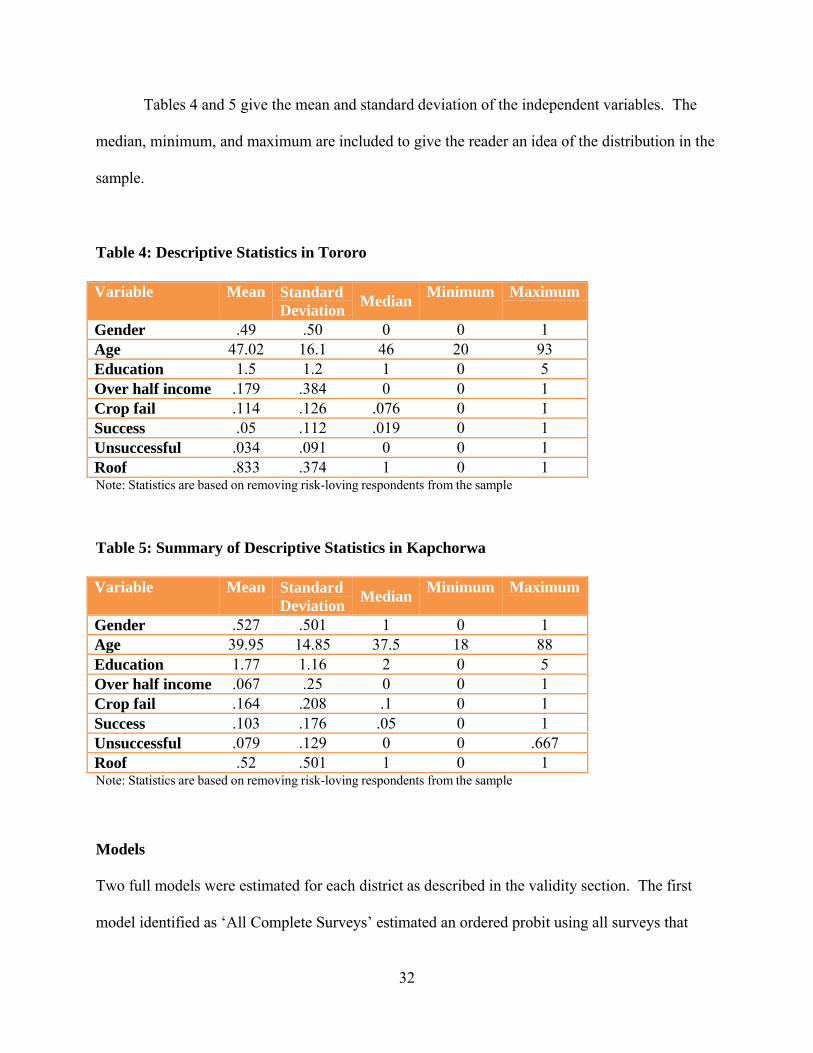
Tables 4 and 5 give the mean and standard deviation of the independent variables. The
median, minimum, and maximum are included to give the reader an idea of the distribution in the
sample.
Table 4: Descriptive Statistics in Tororo
Variable Mean Standard Deviation
MedianMinimum Maximum
Gender .49 .50 0 0 1 Age 47.02 16.1 46 20 93Education 1.5 1.2 1 0 5Over half income .179 .384 0 0 1 Crop fail .114 .126 .076 0 1Success .05 .112 .019 0 1Unsuccessful .034 .091 0 0 1Roof .833 .374 1 0 1 Note: Statistics are based on removing risk-loving respondents from the sample
Table 5: Summary of Descriptive Statistics in Kapchorwa
Variable Mean Standard Deviation
MedianMinimum Maximum
Gender .527 .501 1 0 1Age 39.95 14.85 37.5 18 88Education 1.77 1.16 2 0 5 Over half income .067 .25 0 0 1Crop fail .164 .208 .1 0 1Success .103 .176 .05 0 1 Unsuccessful .079 .129 0 0 .667Roof .52 .501 1 0 1Note: Statistics are based on removing risk-loving respondents from the sample
Models
Two full models were estimated for each district as described in the validity section. The first
model identified as ‘All Complete Surveys’ estimated an ordered probit using all surveys that

33
were completed successfully. In Tororo, six observations lack crucial data. In Kapchorwa, there
were eleven surveys missing a response to a question, primarily gender did not get recorded.
The second model removed observations with respondents who chose the risk-loving lottery (F*)
in the second game and is titled ‘Risk-Loving Respondents Removed’.
The model regressed the risk aversion level on a vector of household attributes thought to
affect a person’s degree of risk aversion:
5) 1 2 3 4
5 6 7 8
9 where Lottery Option is the lottery option chosen and is regressed on gender, age, education
(categorically defined), , over half income (if more than half their income is nonfarm income),
successful, unsuccessful (number of time they tried something new and found it to be successful
or unsuccessful), roof (corrugated steel roof as a proxy for wealth).
In addition to the full models, restricted models were estimated as well; none of which
provided additional insight. Gender, age, and education along with the different wealth
indicators were included. Also the variable of previous success and crop loss were included in
restricted models.
34
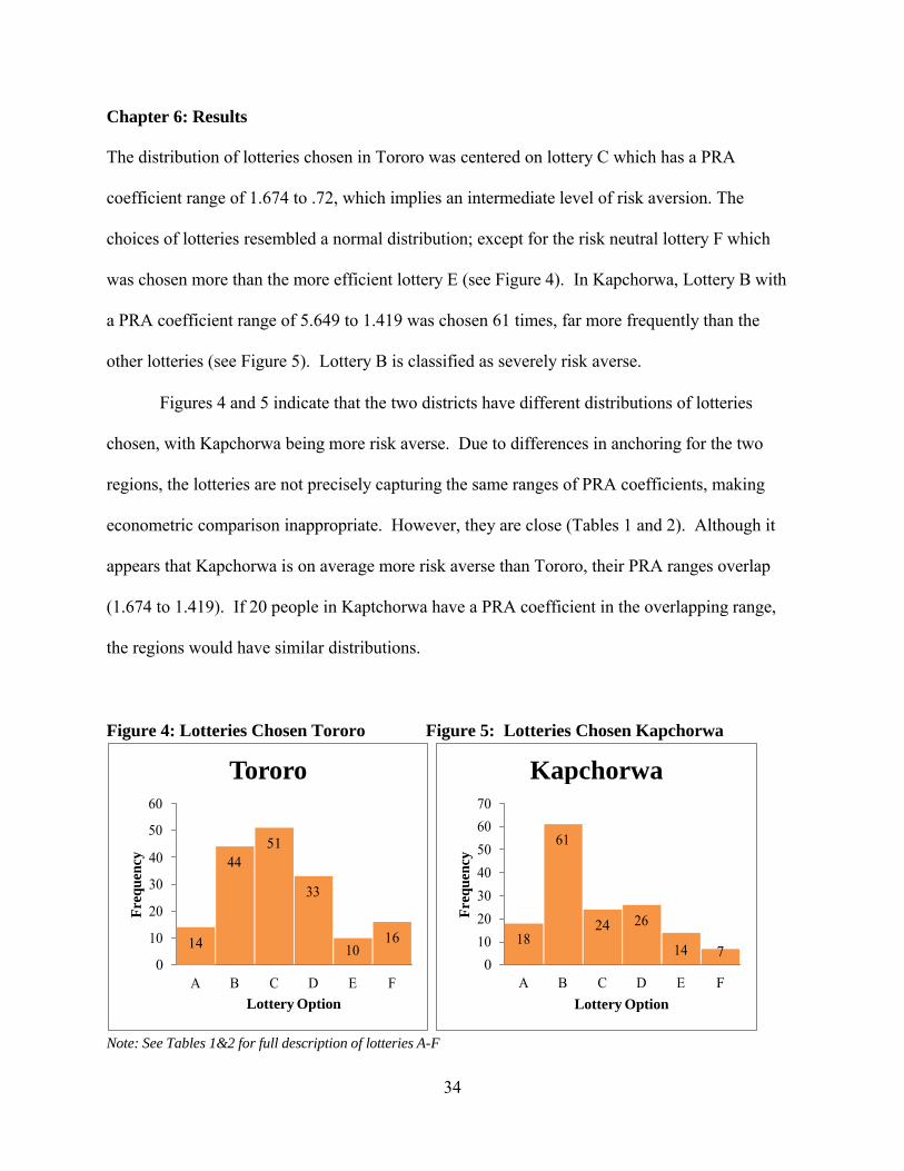
Chapter 6: Results The distribution of lotteries chosen in Tororo was centered on lottery C which has a PRA
coefficient range of 1.674 to .72, which implies an intermediate level of risk aversion. The
choices of lotteries resembled a normal distribution; except for the risk neutral lottery F which
was chosen more than the more efficient lottery E (see Figure 4). In Kapchorwa, Lottery B with
a PRA coefficient range of 5.649 to 1.419 was chosen 61 times, far more frequently than the
other lotteries (see Figure 5). Lottery B is classified as severely risk averse.
Figures 4 and 5 indicate that the two districts have different distributions of lotteries
chosen, with Kapchorwa being more risk averse. Due to differences in anchoring for the two
regions, the lotteries are not precisely capturing the same ranges of PRA coefficients, making
econometric comparison inappropriate. However, they are close (Tables 1 and 2). Although it
appears that Kapchorwa is on average more risk averse than Tororo, their PRA ranges overlap
(1.674 to 1.419). If 20 people in Kaptchorwa have a PRA coefficient in the overlapping range,
the regions would have similar distributions.
Figure 4: Lotteries Chosen Tororo Figure 5: Lotteries Chosen Kapchorwa
Note: See Tables 1&2 for full description of lotteries A-F
14
Tororo 60
50 51
40
30
20
10
0
44
33
1610
A B C D E F
Lottery Option
Kapchorwa 70
60
50
40
30
20
10
0
61
24 26 18
14 7
A B C D E F
Lottery Option
Fre
quen
cy
Fre
quen
cy
35
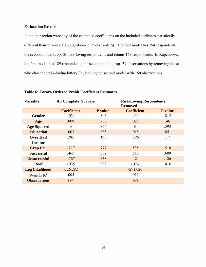
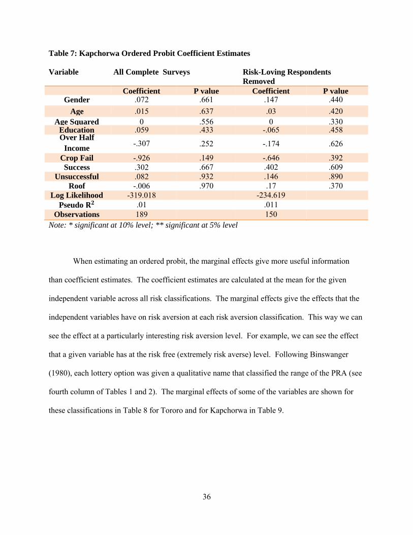
Estimation Results
In neither region were any of the estimated coefficients on the included attributes statistically
different than zero at a 10% significance level (Table 6). The first model has 194 respondents;
the second model drops 26 risk-loving respondents and retains 168 respondents. In Kapchorwa,
the first model has 189 respondents; the second model drops 39 observations by removing those
who chose the risk-loving lottery F*, leaving the second model with 150 observations.
Table 6: Tororo Ordered Probit Coefficient Estimates
Variable All Complete Surveys Risk-Loving Respondents Removed
Coefficient P value Coefficient P value Gender -.031 .846 -.04 .812
Age .009 .736 .021 .46 Age Squared 0 .854 0 .593
Education .003 .963 .015 .841 Over Half
Income .285 .156 .296 .17
Crop Fail -.217 .777 .535 .518 Successful .465 .632 .513 .609
Unsuccessful -.767 .538 -2 .126 Roof -.035 .862 -.184 .416
Log Likelihood -326.282 -271.026
Pseudo .005 .011
Observations 194 168
36
Table 7: Kapchorwa Ordered Probit Coefficient Estimates
Variable All Complete Surveys Risk-Loving Respondents Removed
Coefficient P value Coefficient P valueGender .072 .661 .147 .440
Age .015 .637 .03 .420Age Squared 0 .556 0 .330
Education .059 .433 -.065 .458Over Half
Income -.307
.252 -.174 .626
Crop Fail -.926 .149 -.646 .392Success .302 .667 .402 .609
Unsuccessful .082 .932 .146 .890Roof -.006 .970 .17 .370
Log Likelihood -319.018 -234.619
Pseudo .01 .011
Observations 189 150
Note: * significant at 10% level; ** significant at 5% level
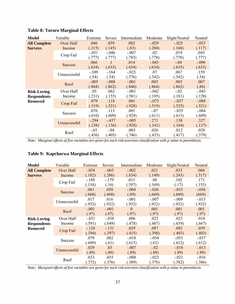
When estimating an ordered probit, the marginal effects give more useful information
than coefficient estimates. The coefficient estimates are calculated at the mean for the given
independent variable across all risk classifications. The marginal effects give the effects that the
independent variables have on risk aversion at each risk aversion classification. This way we can
see the effect at a particularly interesting risk aversion level. For example, we can see the effect
that a given variable has at the risk free (extremely risk averse) level. Following Binswanger
(1980), each lottery option was given a qualitative name that classified the range of the PRA (see
fourth column of Tables 1 and 2). The marginal effects of some of the variables are shown for
these classifications in Table 8 for Tororo and for Kapchorwa in Table 9.
37
Table 8: Tororo Marginal Effects
Model Variable Extreme Severe Intermediate Moderate Slight/Neutral Neutral All Complete Surveys
Over Half Income
.046 (.215)
.059 (.145)
.002 (.83)
-.029 (.204)
-.025 (.168)
-.053 (.117)
Crop Fail -.031 (.777)
-.046 (.777)
-.007 (.783)
.02 (.778)
.019 (.778)
.045 (.777)
Success .066
(.634) .1
(.633) .014
(.654) -.043 (.634)
-.04 (.635)
-.096 (.633)
Unsuccessful -.109 (.54)
-.164 (.54)
-.023 (.576)
.07 (.542)
.067 (.542)
.159 (.54)
Roof -.005 (.864)
-.008 (.862)
-.001 (.846)
.003 (.864)
.003 (.862)
.007 (.86)
Risk-Loving Respondents Removed
Over Half Income
Crop Fail
Success
Roof
Note: Marginal effects of five variables are given for each risk-aversion classification with p value in parenthesis.
Table 9: Kapchorwa Marginal Effects
Model Variable Extreme Severe Intermediate Moderate Slight/Neutral Neutral All Complete Surveys
Over Half Income
-.054 (.182)
-.065 (.286)
-.002 (.834)
.021 (.149)
.033 (.243)
.066 (.317)
Crop Fail -.188 (.154)
-.179 (.16)
.013 (.397)
.08 (.169)
.102 (.17)
.171 (.155)
Success .061
(.668) .058
(.668) -.004 (.69)
-.026 (.669)
-.033 (.669)
-.056 (668)
Unsuccessful .017
(.932) .016
(.932) -.001 (.932)
-.007 (.932)
-.009 (.932)
-.015 (.932)
Roof -.001 (.97)
-.001 (.97)
0 (.97)
.001 (.97)
.001 (.97)
.001 (.97)
Risk-Loving Respondents Removed
Over Half Income
Crop Fail
Success
Roof
Note: Marginal effects of five variables are given for each risk-aversion classification with p value in parenthesis.
Unsuccessful
Unsuccessful
.05 .062 -.001 -.042 -.02 -.043 (.231) (.155) (.581) (.195) (.181) (.128).079 .118 .001 -.073 -.037 -.088
(.519) (.521) (.928) (.519) (.525) (.521).076 .113 .001 -.07 -.035 -.084
(.610) (.609) (.929) (.611) (.613) (.609)-.294 -.437 -.005 .271 .138 .327 (.138) (.136) (.928) (.141) (.164) (.137)-.03 -.04 .003 .026 .012 .028
(.456) (.405) (.746) (.433) (.417) (.379)
-.031 -.038 .006 .022 .023 .018 (.591) (.649) (.478) (.607) (.639) (.667)-.126 -.131 .029 .087 .082 .059 (.394) (.397) (.415) (.398) (.403) (.403).078 .082 -.018 -.054 -.051 -.037
(.609) (.61) (.615) (.61) (.612) (.612).029 .03 -.007 -.02 -.018 -.013 (.89) (.89) (.89) (.89) (.89) (.89).033 .035 -.008 -.023 -.021 -.016
(.372) (.376) (.389) (.376) (.382) (.386)

38
Discussion Farmers who chose lotteries A or B are of most interest since they are classified as extremely and
severely risk averse. These ranges are the most interesting because of their high PRA
coefficients and they are the ones expected to be least likely to adopt CAPs if we assume farmers
are more resistant to adopting new technology the higher their risk aversion. In Tororo, 58
people or 35% of the sample chose a lottery with less risk than lottery C, which is classified as
intermediate risk averse. Of those, 14 or 8% chose lottery A, which has no risk at all. In
Kapchorwa, 79 or 53% chose lottery A or B and 18 or 12% chose lottery A, the risk free lottery.
Those revealing a high level of risk aversion are a substantial percentage of the population and
their risk aversion could slow their adoption of new farming techniques.
If however we assume that CAPs will be adopted by the more risk averse due to their
presumed benefit of decreasing yield variability, then the story of adoption could be switched.
The more risk averse would adopt CAPs for the benefit of reducing production risk. All farmers
would be happy to reduce risk if it does not cost them anything, so if CAPs reduce variability
then all groups will be quick to adopt them based on yield/variation calculations. These two
assumptions prescribe very different estimates for CAPs adoption as it pertains to risk
preference.
The hypothesis that the wealthier are less risk averse is not born out in this data from
eastern Uganda. The models do not find that wealth as represented by roof type has any
correlation with a farmer’s tolerance for risk. These findings agree with most previous studies
(Binswanger, 1980; Cook et al., 2013; Humphrey & Verschoor, 2004) but does not find any
evidence to support the findings of Wik et al. (2004) or Yesuf and Bluffstone (2009). The range
39
of wealth for this data set is limited by wealth differences among the randomly selected Ugandan
farmers. By Ugandan standards, there was a large variation of wealth in the data set, but by
international standards the range was relatively small. The models therefore do not claim that
large amounts of wealth do not have an effect, but that wealth as represented by current wealth
stratification represented by those with improved roofing, animals, or land does not significantly
affect risk aversion. The wealth variable in this study does not capture the entirety of a farmer’s
wealth; future studies might be able to calculate a more complete wealth index. With a more
precise wealth calculation, empirical modeling might find wealth to influence risk aversion.
Also, a more complete wealth calculation could allow for calculation of absolute and relative risk
aversion.
The data estimated here do not support the hypothesis that previous success with
adoption is correlated with decreased risk aversion. This is in contrast to Yesuf and Bluffstone
(2009) who suggest that the poor are path dependent and become more confident and less risk
averse as they experience small successes. This does not mean that if the CAPs being studied in
Uganda are successful that people will not adopt them. What the lack of correlation between
success and risk aversion suggests is that each innovation a farmer tries is judged on its own
merits and the farmer maintains his/her risk aversion level no matter how successful each
innovation turns out to be. Also, this lack of correlation means that an adopter of successful
CAPs will not necessarily be more willing to adopt an unrelated innovation and vise-versa.
There are benefits to CAPs other than yield and variation that are important to adopters. For farmers in Kapchorwa who are farming on very steep land, soil retention is paramount. Even
if the yield and risk-reducing benefits of CAPs are not proven, farmers who have watched their
soil flow down the hill during heavy rains may be anxious to try something that offers any
40
promise of retaining their soil. It may be a hard to convince farmers in Tororo the benefits most
appropriate to them are that minimal soil disturbance and cover crops shade the soil from the sun
and therefore increase the soils ability to retain moisture. It is likely that risk preference as it
pertains to trying something new will be a significant factor in adoption in Tororo but may be
less of a factor to farmers in Kapchorwa.
Conclusions
Will aversion to risk limit the adoption of CAPs in eastern Uganda if SANREM IL researchers
discover that CAPSs are beneficial? 35% of farmers in Tororo and 53% of farmers in
Kapchorwa selected either an extreme or severe risk-averse lottery from the ordered lottery
selection used to measure risk aversion and of those 32, or 14% chose a risk free option. There
is no threshold PRA coefficient that can be used to decipher who will adopt. However, the Z
score provides a ‘price’ of variation in terms of increased yield that can be used to compare
current practice to the mean yield and variation of the new CAPs. This study does not claim to
completely capture how farmers make uncertain decisions, and the risk measurement only
captures mean/variance substitution and misses other real or perceived externalities of CAPs.
Risk aversion may be a barrier to adoption of CAPs and limit the spread of CAPs. However, this
research does not find any the poor view risk differently than their wealthier neighbors. Risk is a
factor all farmers deal with and can be addressed in Uganda based on institutions, laws and
politics present there realizing their poor are not more risk averse than the rest.
No correlation was found between risk preference and any of the demographics collected
from the farmers of eastern Uganda. This hypothetical risk measurement tool obtained similar
findings to Binswager’s results over three decades ago. Higher wealth as measured here did not

41
correlate with a reduced risk aversion. This study agrees with Binswanger that risk aversion is
not innate to poverty. This study used self-reported previous successful and unsuccessful
innovations and found that people are not more willing to take on risk when they have had
previous success, as suggested by Yesuf and Bluffstone. These findings suggest that the poverty
trap identified for the poor, due to their inherent risk aversion, is not evident.
Lipton’s argument that the poor living in fear of a catastrophe that will cause irreparable
harm are inherently more risk averse seems logical, but the research here does not support it.
The risk preferences of the two groups, stratified by roof type, do not have significantly different
distributions. That is not to say that risk is not a major issue for low-income farmers just as it is
for people all over the world. Many people in many places have developed tools to mitigate or
distribute risk, but many of these explicit tools have not found their way into all parts of the
world. The farming decisions of low-income farmers may make it appear that they are more risk
averse, but it is the lack of market structures like those accessible to farmers in developed
countries that make them handle risk differently. When asked how they coped with crop failure,
40% said they obtained a loan from friends or family. Ugandans have informal tools for dealing
with risks that are ex-post rather than ex-ante. One man summed up what many farmers said
while talking about how they smooth their consumption after a catastrophic crop failure: “we
have ways of dealing with crop loss; it’s ok”. Even though farmers in eastern Uganda lack
strong market structures to manage risk, they still are anxious to try new things that may be
promising in spite of risk. This survey of eastern Uganda found many people anxious to learn
about CAPs that might help maintain quality soil, reduce erosion, and minimize weeds and labor
costs; they did not seem fearful of trying something new.

42
References Anderson, J. R. D. J. L. F., & Agriculture Organization of the United, N. (1992). Risk analysis in
dryland farming systems. Rome: Food and Agriculture Organization of the United
Nations.
Binswanger, H. P. (1980). Attitudes toward Risk: Experimental Measurement In Rural India.
American Journal of Agricultural Economics, 62(3), 395. Cook, J., Chatterjee, S., Sur, D., & Whittington, D. (2013). Measuring risk aversion among the
urban poor in Kolkata, India. Applied Economics Letters, 20(1), 1-9. doi:
10.1080/13504851.2011.644235
Harrison, G. W., Humphrey, S. J., & Verschoor, A. (2010). Choice under Uncertainty: Evidence
from Ethiopia, India and Uganda. Economic Journal, 120(543), 80-104. doi:
10.1111/j.1468-0297.2009.02303.x
Hopper, W. D. (1965). Allocation Efficiency in a Traditional Indian Agriculture. Journal of
Farm Economics, 47(3), 611-624. doi: 10.2307/1236276
Humphrey, S. J., & Verschoor, A. (2004). Decision-making Under Risk among Small Farmers in
East Uganda. Journal of African Economies, 13(1), 44-101. doi: 10.1093/jae/13.1.44
Lamb, J. (2011). Food Security and Social Networks: Impacts for Smallholder Farmers in the
Mount Elgon Region of Kenya and Uganda. (Master), Virginia Tech.
Lipton, M. (1968). The Theory of Optimising Peasant. Journal of Development Studies, 4(3), 26.
Miyata, S. (2003). Household's risk attitudes in Indonesian villages. Applied Economics, 35(5),
573. doi: 10.1080/0003684022000020823
43
Mosley, P., & Verschoor, A. (2005). Risk Attitudes and the ‘Vicious Circle of Poverty’.
European Journal of Development Research, 17(1), 59-88. doi:
10.1080/09578810500066548
Pratt, J. W. (1964). Risk Aversion in the Small and in the Large. Econometrica, 32(1/2), 122-
136. doi: 10.2307/1913738
Roumasset, J. A. B. J.-M. S. I. S. A. R. C. f. G. S., & Research in Agriculture, A. D. C. (1979).
Risk, uncertainty, and agricultural development. College, Laguna, Philippines; New
York, N.Y.: Southeast Asian Regional Center for Graduate Study and Research in
Agriculture ; Agricultural Development Council.
Schultz, T. W. (1964). Transforming traditional agriculture. New Haven: Yale University Press. Wik, M., Kebede, T. A., Bergland, O., & Holden, S. T. (2004). On the measurement of risk
aversion from experimental data. Applied Economics, 36(21), 2443-2451. doi:
10.1080/0003684042000280580
Yesuf, M., & Bluffstone, R. A. (2009). Poverty, Risk Aversion, and Path Dependence in Low-
Income Countries: Experimental Evidence from Ethiopia. American Journal of
Agricultural Economics, 91(4), 1022-1037. doi: 10.1111/j.1467-8276.2009.01307.x
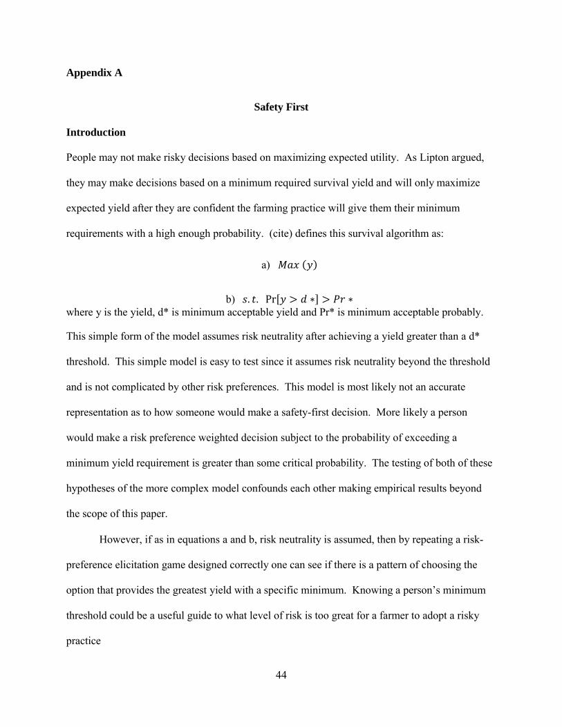
44
Appendix A
Safety First
Introduction People may not make risky decisions based on maximizing expected utility. As Lipton argued,
they may make decisions based on a minimum required survival yield and will only maximize
expected yield after they are confident the farming practice will give them their minimum
requirements with a high enough probability. (cite) defines this survival algorithm as:
a)
b) . . Pr ∗ ∗where y is the yield, d* is minimum acceptable yield and Pr* is minimum acceptable probably.
This simple form of the model assumes risk neutrality after achieving a yield greater than a d*
threshold. This simple model is easy to test since it assumes risk neutrality beyond the threshold
and is not complicated by other risk preferences. This model is most likely not an accurate
representation as to how someone would make a safety-first decision. More likely a person
would make a risk preference weighted decision subject to the probability of exceeding a
minimum yield requirement is greater than some critical probability. The testing of both of these
hypotheses of the more complex model confounds each other making empirical results beyond
the scope of this paper.
However, if as in equations a and b, risk neutrality is assumed, then by repeating a risk-
preference elicitation game designed correctly one can see if there is a pattern of choosing the
option that provides the greatest yield with a specific minimum. Knowing a person’s minimum
threshold could be a useful guide to what level of risk is too great for a farmer to adopt a risky
practice
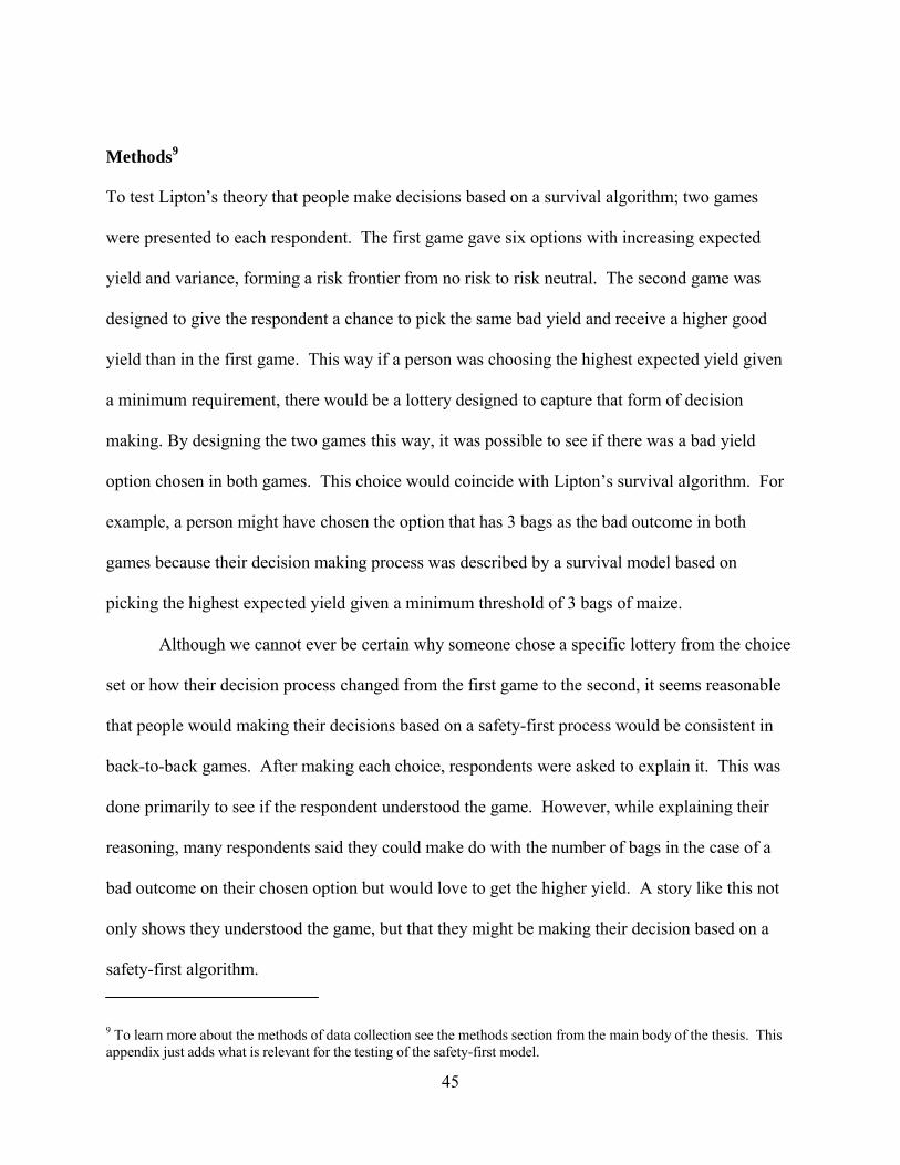
45
Methods9
To test Lipton’s theory that people make decisions based on a survival algorithm; two games
were presented to each respondent. The first game gave six options with increasing expected
yield and variance, forming a risk frontier from no risk to risk neutral. The second game was
designed to give the respondent a chance to pick the same bad yield and receive a higher good
yield than in the first game. This way if a person was choosing the highest expected yield given
a minimum requirement, there would be a lottery designed to capture that form of decision
making. By designing the two games this way, it was possible to see if there was a bad yield
option chosen in both games. This choice would coincide with Lipton’s survival algorithm. For
example, a person might have chosen the option that has 3 bags as the bad outcome in both
games because their decision making process was described by a survival model based on
picking the highest expected yield given a minimum threshold of 3 bags of maize.
Although we cannot ever be certain why someone chose a specific lottery from the choice
set or how their decision process changed from the first game to the second, it seems reasonable
that people would making their decisions based on a safety-first process would be consistent in
back-to-back games. After making each choice, respondents were asked to explain it. This was
done primarily to see if the respondent understood the game. However, while explaining their
reasoning, many respondents said they could make do with the number of bags in the case of a
bad outcome on their chosen option but would love to get the higher yield. A story like this not
only shows they understood the game, but that they might be making their decision based on a
safety-first algorithm.
9 To learn more about the methods of data collection see the methods section from the main body of the thesis. This appendix just adds what is relevant for the testing of the safety-first model.
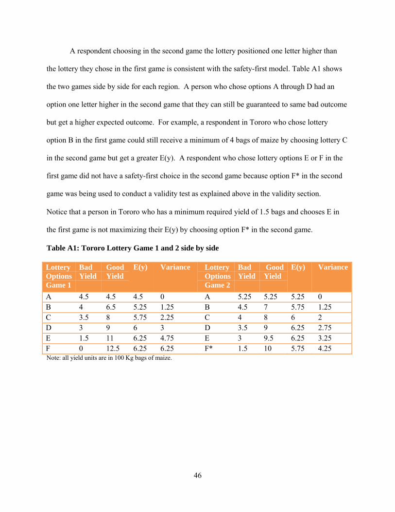
46
A respondent choosing in the second game the lottery positioned one letter higher than
the lottery they chose in the first game is consistent with the safety-first model. Table A1 shows
the two games side by side for each region. A person who chose options A through D had an
option one letter higher in the second game that they can still be guaranteed to same bad outcome
but get a higher expected outcome. For example, a respondent in Tororo who chose lottery
option B in the first game could still receive a minimum of 4 bags of maize by choosing lottery C
in the second game but get a greater E(y). A respondent who chose lottery options E or F in the
first game did not have a safety-first choice in the second game because option F* in the second
game was being used to conduct a validity test as explained above in the validity section.
Notice that a person in Tororo who has a minimum required yield of 1.5 bags and chooses E in
the first game is not maximizing their E(y) by choosing option F* in the second game.
Table A1: Tororo Lottery Game 1 and 2 side by side
Lottery Options Game 1
Bad Yield
Good Yield
E(y) Variance Lottery Options Game 2
Bad Yield
Good Yield
E(y) Variance
A 4.5 4.5 4.5 0 A 5.25 5.25 5.25 0B 4 6.5 5.25 1.25 B 4.5 7 5.75 1.25 C 3.5 8 5.75 2.25 C 4 8 6 2D 3 9 6 3 D 3.5 9 6.25 2.75E 1.5 11 6.25 4.75 E 3 9.5 6.25 3.25 F 0 12.5 6.25 6.25 F* 1.5 10 5.75 4.25Note: all yield units are in 100 Kg bags of maize.

47
Table A2: Kapchorwa Lottery Game 1 and 2 side by side
Lottery Options Game 1
Bad Good E(y) Variance Lottery Options Game 2
Bad Good E(y) Variance
A 15 15 15 0 A 20.5 20.5 20.5 0 B 13 28 20.5 7.5 B 15 32 23.5 8.5C 11 36 23.5 12.5 C 13 35 24 11D 10 38 24 14 D 11 38 24.5 13.5 E 8 41 24.5 16.5 E 10 39 24.5 14.5F 6 43 24.5 18.5 F* 8 40 24 16Note: all yield units are in 100 Kg bags of maize.
In the context of the lottery list, the probability of a bad or good outcome was always
50%; therefore the critical probability (Pr*) of the safety-first model was fixed and d* was the
only variable in the constraint. Since the objective of the safety-first model assumes risk
neutrality subject to meeting a minimum requirement, and the curvature of the game assumes
risk aversion, the safety first model suggests a person will choose the highest yielding and
subsequently riskiest lottery they can as long as the bad outcome does not drop lower than their
d*.
The assumption that people are risk neutral after satisfying a safety-first constraint is
unlikely. It is more likely that people balance their risk preferences and minimum requirements
simultaneously. It is difficult to test a safety-first constraint while relaxing the risk neutrality
assumption and allowing for risk preferences in the objective. Testing the decision making
process and risk preferences confound each other. Therefore, as an alternative, these two aspects
of choice under uncertainty were analyzed by taking the EUT risk preference in game 1 and
examining the results of the respondents who chose a lottery in game 2 that was consistent with
the safety-first model. This meant that respondents choosing lottery A in the first game then B in
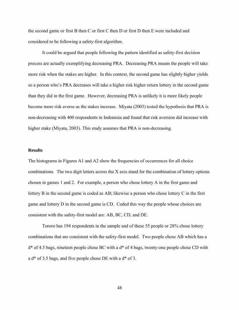
48
the second game or first B then C or first C then D or first D then E were included and
considered to be following a safety-first algorithm.
It could be argued that people following the pattern identified as safety-first decision
process are actually exemplifying decreasing PRA. Decreasing PRA means the people will take
more risk when the stakes are higher. In this context, the second game has slightly higher yields
so a person who’s PRA decreases will take a higher risk higher return lottery in the second game
than they did in the first game. However, decreasing PRA is unlikely it is more likely people
become more risk averse as the stakes increase. Miyata (2003) tested the hypothesis that PRA is
non-decreasing with 400 respondents in Indonesia and found that risk aversion did increase with
higher stake (Miyata, 2003). This study assumes that PRA is non-decreasing.
Results
The histograms in Figures A1 and A2 show the frequencies of occurrences for all choice
combinations. The two digit letters across the X axis stand for the combination of lottery options
chosen in games 1 and 2. For example, a person who chose lottery A in the first game and
lottery B in the second game is coded as AB; likewise a person who chose lottery C in the first
game and lottery D in the second game is CD. Coded this way the people whose choices are
consistent with the safety-first model are: AB, BC, CD, and DE.
Tororo has 194 respondents in the sample and of these 55 people or 28% chose lottery
combinations that are consistent with the safety-first model. Two people chose AB which has a
d* of 4.5 bags, nineteen people chose BC with a d* of 4 bags, twenty-one people chose CD with
a d* of 3.5 bags, and five people chose DE with a d* of 3.
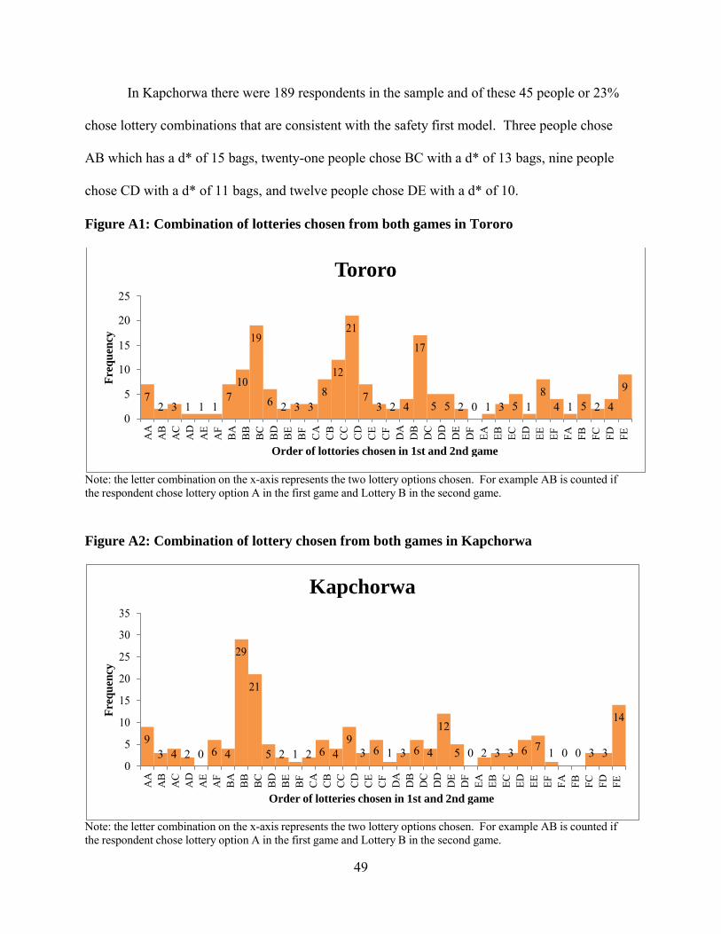
49
Tororo25 20
21
15 10
19 17
1210
5 7 7 8 7 8 9
2 3 1 1 1 6 2 3 3 3 2 4 5 5 2 0 1 3 5 1 4 1 5 2 40
Order of lottories chosen in 1st and 2nd game
Kapchorwa35
30
25
20
15
10
5
0
29
21
9 93 4 2 0 6 4 5 2 1 2 6 4
12
3 6 1 3 6 4 5 0 2 3 3 6 7 1 0 0 3 3
14
Order of lotteries chosen in 1st and 2nd game
In Kapchorwa there were 189 respondents in the sample and of these 45 people or 23%
chose lottery combinations that are consistent with the safety first model. Three people chose
AB which has a d* of 15 bags, twenty-one people chose BC with a d* of 13 bags, nine people
chose CD with a d* of 11 bags, and twelve people chose DE with a d* of 10.
Figure A1: Combination of lotteries chosen from both games in Tororo
Note: the letter combination on the x-axis represents the two lottery options chosen. For example AB is counted if the respondent chose lottery option A in the first game and Lottery B in the second game.
Figure A2: Combination of lottery chosen from both games in Kapchorwa
Note: the letter combination on the x-axis represents the two lottery options chosen. For example AB is counted if the respondent chose lottery option A in the first game and Lottery B in the second game.
Fre
quen
cy
Fre
quen
cy
AA
A
B
AC
A
D
AE
A
F B
A
BB
B
C
BD
B
E
BF
C
A
CB
C
C
CD
C
E
CF
D
A
DB
D
C
DD
D
E
DF
EA
E
B
EC
E
D
EE
E
F FA
F
B
FC
FD
FE
AA
A
B
AC
A
D
AE
A
F B
A
BB
B
C
BD
B
E
BF
C
A
CB
C
C
CD
C
E
CF
D
A
DB
D
C
DD
D
E
DF
EA
E
B
EC
E
D
EE
E
F FA
F
B
FC
FD
FE
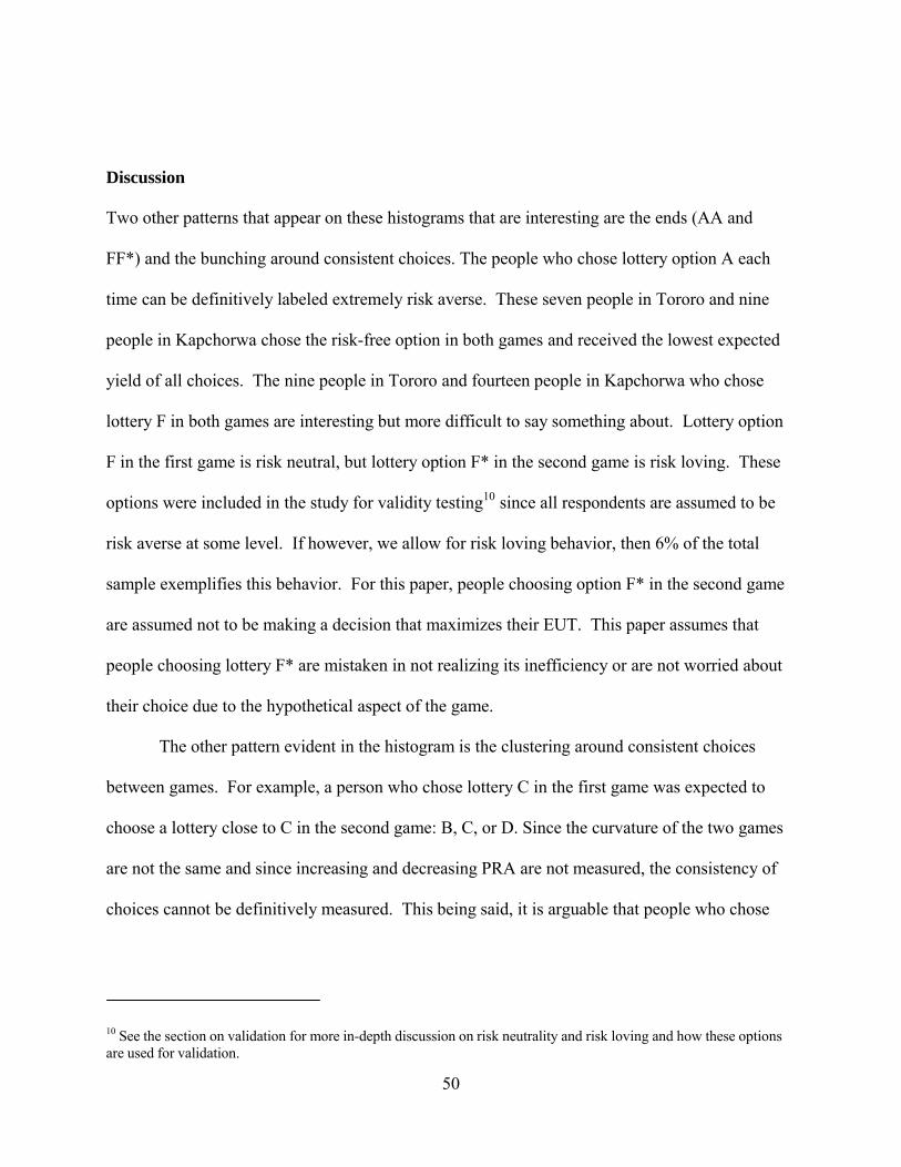
50
Discussion
Two other patterns that appear on these histograms that are interesting are the ends (AA and
FF*) and the bunching around consistent choices. The people who chose lottery option A each
time can be definitively labeled extremely risk averse. These seven people in Tororo and nine
people in Kapchorwa chose the risk-free option in both games and received the lowest expected
yield of all choices. The nine people in Tororo and fourteen people in Kapchorwa who chose
lottery F in both games are interesting but more difficult to say something about. Lottery option
F in the first game is risk neutral, but lottery option F* in the second game is risk loving. These
options were included in the study for validity testing10 since all respondents are assumed to be
risk averse at some level. If however, we allow for risk loving behavior, then 6% of the total
sample exemplifies this behavior. For this paper, people choosing option F* in the second game
are assumed not to be making a decision that maximizes their EUT. This paper assumes that
people choosing lottery F* are mistaken in not realizing its inefficiency or are not worried about
their choice due to the hypothetical aspect of the game.
The other pattern evident in the histogram is the clustering around consistent choices
between games. For example, a person who chose lottery C in the first game was expected to
choose a lottery close to C in the second game: B, C, or D. Since the curvature of the two games
are not the same and since increasing and decreasing PRA are not measured, the consistency of
choices cannot be definitively measured. This being said, it is arguable that people who chose
10 See the section on validation for more in-depth discussion on risk neutrality and risk loving and how these options are used for validation.

51
the risk-free lottery in the first game (A) and the risk-loving option (F*) in the second game are
not presenting a stable risk preference.
Conclusion
There were approximately a quarter of the respondents whose choices from the two risk-
elicitation games were consistent with the safety-first model. These people can be assumed to be
making their decision based on a safety-first algorithm if a strict non-decreasing PRA is adhered
to. However, the lottery in the second game that corresponds to a safety-first decision is not very
different from the lottery in the first game and could be interpreted as a consistent EUT choice.
Realizing that the same choice sets that are consistent with safety-first model are almost
consistent with a stable EUT choice decision makes it difficult to say much about their decision
making process. Even when strict non-decreasing EUT is assumed there are still only a quarter of
the people who exemplify safety-first algorithm and their d* is as diverse as possible given the
lottery choices.
There does not appear to be much evidence that eastern Ugandan farmers make their
uncertain decisions based on the specified safety-first model. Considering those that did make
safety-first lottery choices, the minimum threshold (d*) they exemplified is not homogeneous
enough to be useful in suggesting what minimum yield CAPs must attain to satisfy the safety-
first constraint. The EUT analysis of this paper agreed with Binswanger’s empirical findings
from three decades ago that risk aversion is not innate in poverty and this appendix does not find
much evidence to support Lipton’s theory either. Therefore, agricultural development agencies
in less-developed countries should not think of farmers’ risk aversion any different than any
farmer living with constraints and market structures in place. There is no increased risk aversion
52
innate in poverty; subsistence farmers are mitigating risk the best they can with the information,
resource, and institutions in place where they live.
This was put in an appendix due to the difficulty of empirically testing if people make
decisions based on a safety-first algorithm. There could be a great amount of work done using
behavior economics that could parcel out risk aversion and minimum threshold as well as real
compared to perceived risk. Another difficulty of this research that could be tested is how an
empirically tested risk aversion correlated to the adoption of higher-risk higher-return
investments.

53
Appendix B
Uganda Survey
Uganda Survey Respondent ID:
District : Sub-County: Village:
Name of Interviewers: _ Date:
Gender of respondent: Male Female
Hello, my name is , and this is and . We are
conducting research for the SANREM Project, which has many institutions involved, including
Makerere University, Appropriate Technology, and universities in the United States. We would
like to ask you questions about your household farming decisions. Would you be willing to
participate in this survey? Participation in this survey is voluntary and the answers that you
provide will be anonymous and confidential.
This survey will take about 1 hour. Do you agree to participate in this survey? YES NO
1) Do you make farming decisions for your household? YES NO
o (If there is no person to make farming decision go on to the next farm)
2) What is your age?
3) How many years of school have you completed?
4) How many people in total are in your household?
5) How many people in your household work on your farm?
6) How many people in your household are under 13 years old?
7) How many years have you worked on a farm?
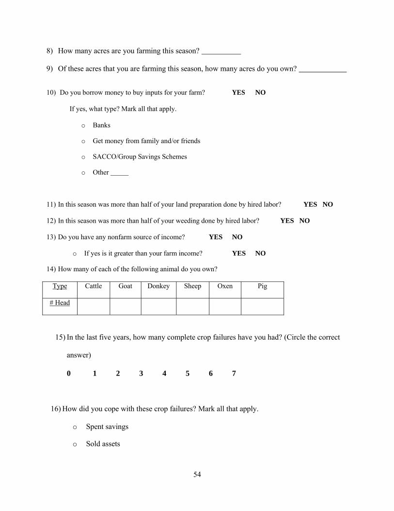
54
8) How many acres are you farming this season?
9) Of these acres that you are farming this season, how many acres do you own?
10) Do you borrow money to buy inputs for your farm? YES NO
If yes, what type? Mark all that apply.
o Banks
o Get money from family and/or friends
o SACCO/Group Savings Schemes
o Other
11) In this season was more than half of your land preparation done by hired labor? YES NO
12) In this season was more than half of your weeding done by hired labor? YES NO
13) Do you have any nonfarm source of income? YES NO
o If yes is it greater than your farm income? YES NO
14) How many of each of the following animal do you own?
Type Cattle Goat Donkey Sheep Oxen Pig
# Head
15) In the last five years, how many complete crop failures have you had? (Circle the correct
answer)
0 1 2 3 4 5 6 7
16) How did you cope with these crop failures? Mark all that apply.
o Spent savings
o Sold assets

55
o Reduced consumption
o Bank Loan
o Got help from family and/or friends
o Other
17) In the last five years, how many times have you tried something new on your farm that you
considered to be successful? For example, a new crop variety, a new fertilizer, a new piece of
equipment.
18) In the last five years, how many times have you tried something new on your farm that did
not meet your expectations? For example, a new crop variety, a new fertilizer, a new piece of
equipment.
19) Which of these crops did you plant on your farm this season? Circle all that apply.
MAIZE BEANS CASSAVA GROUNDNUTS IRISH POTATOES
SWEET POTATOES VEGETABLES FRUIT 20) Have you ever practiced minimum tillage? YES NO
o If yes, do you still practice minimum tillage? YES NO
21) Have you ever grown a cover crop? YES NO
o If yes, do you still grow a cover crop? YES NO
22) Have you ever practiced crop rotations? YES NO

56
o If yes, do you still practice crop rotations? YES NO
23) Do you view soil erosion as a problem on your land? YES NO 24) Are you doing something to manage erosion? YES NO
25) Type of roof on house:
THATCHED TIN IRON SHEET TILE OTHER
26) Type of floor in house:
MUD FLOOR CEMENT TILE OTHER
27) Number of rooms in house:
Choice Survey # 1: Risk
As you know, maize production is risky. When you plant maize you cannot be certain how much
maize you will eventually harvest. For this question we will show you 6 different possibilities for
maize yields on one acre. Assume you have a 50/50 (or equal) chance of a good harvest or bad
harvest. We are interested in which yield possibility sounds best to you.
*Do the practice game with three options. Have respondent play the game, using a coin/object in
one hand and have them choose a hand.
Practice Game
Which option did the person pick? A B C

57
Did the person win the game ? YES NO *Once you feel confident that the person understands the way the game is played explain that we
want them to think about what it means for them to live with the outcome of the different choices.
We will now show you a paper with 6 choices of different yield outcomes. When making this
decision we would like you consider the consequences your choice would have on your family
and make this decision the same way you would make a planting decision. When picking an
option please consider how your life would be if the harvest is good and if the harvest is bad.
What option did the respondent choose for Game 1? (A-F)
What option did the respondent choose for Game 2? (A-F)