Embed Size (px)
Citation preview

Techniques for circuit simulation
M. B. Patilwww.ee.iitb.ac.in/~sequel
Department of Electrical EngineeringIndian Institute of Technology Bombay
M. B. Patil, IIT Bombay

Outline
* Circuit simulation: introduction
* Nodal analysis
* Modified nodal analysis
* Sparse tableau approach
* Nonlinear circuits
* Transient (dynamic) analysis
M. B. Patil, IIT Bombay

Circuit simulation
* DC analysis
* transient (time-domain) analysis
* AC (frequency-domain) analysis
* logic-level simulation
* mixed-signal simulation
* noise computation
* periodic steady state computation
* sensitivity analysis
M. B. Patil, IIT Bombay

Why do we need circuit simulation?
R1
R2Vs
is
Example 1
M. B. Patil, IIT Bombay

Why do we need circuit simulation?
R1
R2R3Vs
is
Example 1
M. B. Patil, IIT Bombay

Why do we need circuit simulation?
R1
R2R3Vs
is
R4
Example 1
M. B. Patil, IIT Bombay

Why do we need circuit simulation?
R1
R2R3Vs
is
R4
R5
Example 1
M. B. Patil, IIT Bombay

Why do we need circuit simulation?
R1
R2R3
R6Vs
is
R4
R5
Example 1
M. B. Patil, IIT Bombay

Why do we need circuit simulation?
VC1
Vs(t)
R1
C1
Example 2
M. B. Patil, IIT Bombay

Why do we need circuit simulation?
VC1
Vs(t)
R1
C1
Example 2
M. B. Patil, IIT Bombay

Why do we need circuit simulation?
VC1
Vs(t)
R1 R2
C1 C2
Example 2
M. B. Patil, IIT Bombay

Why do we need circuit simulation?
VC1
Vs(t)
D R3
R1 R2
C1 C2
Example 2
M. B. Patil, IIT Bombay

Circuit simulation on a computer
* Must be efficient in terms of CPU time (especially for large circuits).
* Must make good use of the memory available. If a matrix is sparse,it should not be stored in the a(i , j) form.
* The approach must be systematic. “Tricks” such as resistors inseries or parallel, star-to-delta conversion, etc. will work in specialcases. What we need is a general-purpose method that will work forall circuits.
M. B. Patil, IIT Bombay

Outline
* Circuit simulation: introduction
* Nodal analysis
* Modified nodal analysis
* Sparse tableau approach
* Nonlinear circuits
* Transient (dynamic) analysis
M. B. Patil, IIT Bombay

Nodal Analysis of a linear circuit
* Take some node as the “reference node” and denotethe node voltages of the remaining nodes by e1 , e2 ,etc.
* Write KCL at each node in terms of the nodevoltages. Follow a fixed convention, e.g., currentleaving a node is positive.
* When all KCL equations are treated, we have the“admittance matrix” and the RHS vector.
* Solve the resulting linear system of equations,Ye = Is for the node voltages.
* The equation assembly (also called “parsing”) can bedone element-by-element, i.e., by considering one lineof the circuit file at a time.
* The computer cannot see the entire circuit; it can,however, go through the circuit file line by line.
Ik v3
e1e
e
2
3
v30
R1
R23R
4R0
SPICE file
I0 1 0 1mR1 1 2 1kR2 2 0 1.2kR3 2 3 200R4 0 3 1kVCCS1 1 3 2 3 0.5m
M. B. Patil, IIT Bombay

Step 1: Initialize
Ik v3
0 0 0
0 0 0
0 0 0e1
e
e
2
3
v30
R1
R23R
4R0
e
e
e
1
2
3
0
0
2
3
KCL at 1 0
M. B. Patil, IIT Bombay

Step 2
Ik v3
0 0 0
0 0 0
0 0 0e1
e
e
2
3
v30
R1
R23R
4R0
e
e
e
1
2
3
0
0
2
3
KCL at 1 0
M. B. Patil, IIT Bombay

Step 2
Ik v3
0 0 0
0 0 0
0 0 0 I0e1e
e
2
3
v30
R1
R23R
4R0
e
e
e
1
2
3
0
0
2
3
KCL at 1
M. B. Patil, IIT Bombay

Step 3
Ik v3
0 0 0
0 0 0
0 0 0 I0e1e
e
2
3
v30
R1
R23R
4R0
e
e
e
1
2
3
0
0
2
3
KCL at 1
M. B. Patil, IIT Bombay

Step 3
Ik v3
0 0 0
I0G1 G1
G1 G1
e1e
e
2
3
v30
R1
R23R
4R0
e
e
e
1
2
3
0
0
2
3
KCL at 1 0
0
M. B. Patil, IIT Bombay

Step 4
Ik v3
0 0 0
I0G1 G1
G1 G1
e1e
e
2
3
v30
R1
R23R
4R0
e
e
e
1
2
3
0
0
2
3
KCL at 1 0
0
M. B. Patil, IIT Bombay

Step 4
Ik v3
0 0 0
I0G1
G1 G +G1 2
e1e
e
2
3
v30
R1
R23R
4R0
e
e
e
1
2
3
0
0
2
3
KCL at 1 0
0
G1
M. B. Patil, IIT Bombay

Step 5
Ik v3
0 0 0
I0G1
G1 G +G1 2
e1e
e
2
3
v30
R1
R23R
4R0
e
e
e
1
2
3
0
0
2
3
KCL at 1 0
0
G1
M. B. Patil, IIT Bombay

Step 5
Ik v3
I0
G1
G1 G1
G +G1 2G3
G3
G3
G3
e1e
e
2
3
v30
R1
R23R
4R0
e
e
e
1
2
3
0
0
2
3
KCL at 1 0
0
M. B. Patil, IIT Bombay

Step 6
Ik v3
I0
G1
G1 G1
G +G1 2G3
G3
G3
G3
e1e
e
2
3
v30
R1
R23R
4R0
e
e
e
1
2
3
0
0
2
3
KCL at 1 0
0
M. B. Patil, IIT Bombay

Step 6
Ik v3
I0
G1
G1 G1
G +G1 2G3
G3
G3 G +G3 4
e1e
e
2
3
v30
R1
R23R
4R0
e
e
e
1
2
3
0
0
2
3
KCL at 1 0
0
M. B. Patil, IIT Bombay

Step 7
Ik v3
I0
G1
G1 G1
G +G1 2G3
G3
G3 G +G3 4
e1e
e
2
3
v30
R1
R23R
4R0
e
e
e
1
2
3
0
0
2
3
KCL at 1 0
0
M. B. Patil, IIT Bombay

Step 7
Ik v3
I0
G1
G1
G +G1 2G3
3G +k G +G3 4
G k1e1e
e
2
3
v30
R1
R23R
4R0
e
e
e
1
2
3
0
0
2
3
KCL at 1
0
G3
k
k
M. B. Patil, IIT Bombay

Outline
* Circuit simulation: introduction
* Nodal analysis
* Modified nodal analysis
* Sparse tableau approach
* Nonlinear circuits
* Transient (dynamic) analysis
M. B. Patil, IIT Bombay

Modified Nodal Analysis (MNA) of a linear circuit
+
e1e2 e3
R1
2R 3R
v2
0V v2
0
i i1 2
α
* When a voltage source is involved, we cannot write its current in terms ofnode voltages (e1, e2, etc.). The NA approach has to be modified ⇒MNA.
* Treat the current through the voltage source as an additional unknown.
* We also need to get an additional equation since the number of unknownshas gone up by 1. This equation is provided by the branch equation of thevoltage source.
* The “solution vector” now contains the voltage source currents inaddition to the node voltages.
M. B. Patil, IIT Bombay

Modified Nodal Analysis of a linear circuit
+
e1e2 e3
R1
2R 3R
v2
0V v2
i1 i2
i1
i2
0
α
e
e
e
1
2
3
KCL at 1
KCL at 2
BCE for VS2
BCE for VS1
KCL at 3
VS1 VS2
M. B. Patil, IIT Bombay

Modified Nodal Analysis of a linear circuit
+
e1e2 e3
R1
2R 3R
v2
0V v2
i1 i2
i1
i2
0
α
e
e
e
1
2
3
KCL at 1
KCL at 2
BCE for VS2
BCE for VS1
KCL at 3
VS1 VS2
G1
M. B. Patil, IIT Bombay

Modified Nodal Analysis of a linear circuit
+
e2 e32R 3R
v2
0V v2
i1 i2
i1
i2
G2
G2
R1
0
α
e
e
e
1
2
3
1 2
2
G +GKCL at 1
KCL at 2
BCE for VS2
BCE for VS1
KCL at 3
VS1 VS2
e1
G
M. B. Patil, IIT Bombay

Modified Nodal Analysis of a linear circuit
+
e1e2
R1
2R 3R
v2
0V v2
i1
i2
G2 G3
G3
G2
i1
0
α
e
e
e
1
2
3G3
1 2
G +G2 3
G +GKCL at 1
KCL at 2
BCE for VS2
BCE for VS1
KCL at 3
VS1 VS2
i2
e3
M. B. Patil, IIT Bombay

Modified Nodal Analysis of a linear circuit
+
i1
i2
G2 G3
G3
G2
e1e2 e3
R1
2R 3R
v2
0V v2
i1 i2
e
e
e
1
2
3
1
G3
1 V0
1 2
G +G2 3
G +GKCL at 1
KCL at 2
BCE for VS2
BCE for VS1
KCL at 3
0
α
VS1 VS2
M. B. Patil, IIT Bombay

Modified Nodal Analysis of a linear circuit
+
i1
i2
G2 G3
G3
G2
e1e2 e3
R1
2R 3R
v2
0V v2
i1 i2
e
e
e
1
2
3
1
G3 1
1
1αα
V0
1 2
G +G2 3
G +GKCL at 1
KCL at 2
BCE for VS2
BCE for VS1
KCL at 3
0
α
VS1 VS2
M. B. Patil, IIT Bombay

Outline
* Circuit simulation: introduction
* Nodal analysis
* Modified nodal analysis
* Sparse tableau approach
* Nonlinear circuits
* Transient (dynamic) analysis
M. B. Patil, IIT Bombay

Sparse Tableau Analysis (STA)
* Variables: node voltages, branch currents, and branch voltages
* No need for special treatment of voltage sources or any otherelements
* Circuit topology and element equations are decoupled.
* Easier to implement as compared to MNA
M. B. Patil, IIT Bombay

Sparse Tableau Analysis (STA)
* Variables: node voltages, branch currents, and branch voltages
* No need for special treatment of voltage sources or any otherelements
* Circuit topology and element equations are decoupled.
* Easier to implement as compared to MNA
M. B. Patil, IIT Bombay

Sparse Tableau Analysis (STA)
* Variables: node voltages, branch currents, and branch voltages
* No need for special treatment of voltage sources or any otherelements
* Circuit topology and element equations are decoupled.
* Easier to implement as compared to MNA
M. B. Patil, IIT Bombay

Sparse Tableau Analysis (STA)
* Variables: node voltages, branch currents, and branch voltages
* No need for special treatment of voltage sources or any otherelements
* Circuit topology and element equations are decoupled.
* Easier to implement as compared to MNA
M. B. Patil, IIT Bombay

−1
11
1
1
−1−1
1
11 −α
1−R
ii
vvvvvv
1
2
3
4
5
6
1
2
3
4
5
6
2−R3
−R2
i
iii
1
4 0V
−I03
VVVV
0
0
0
1
11
1
1
1
−1−1
−1−1
−1 1 11−1
11 1
11
STAexample
v64v
v5
v3
v2
2V 3V V4
i5
V0
i4R3i6i3
v4
i2R2
R1
v1
i1V1
α
0
I0
M. B. Patil, IIT Bombay

−1
11
1
1
−1−1
1
11 −α
1−R
ii
vvvvvv
1
2
3
4
5
6
1
2
3
4
5
6
2−R3
−R2
i
iii
1
4 0V
−I03
VVVV
0
0
0
1
11
1
1
1
−1−1
−1−1
−1 1 11−1
11 1
11
STAexample
v64v
v5
KCL
v3
v2
2V 3V V4
i5
V0
i4R3i6i3
v4
i2R2
R1
v1
i1V1
α
0
I0
M. B. Patil, IIT Bombay

−1
11
1
1
−1−1
1
11 −α
1−R
ii
vvvvvv
1
2
3
4
5
6
1
2
3
4
5
6
2−R3
−R2
i
iii
1
4 0V
−I03
VVVV
0
0
0
1
11
1
1
1
−1−1
−1−1
−1 1 11−1
11 1
11Branch Voltage
Definition
STAexample
v64v
v5
KCL
v3
v2
2V 3V V4
i5
V0
i4R3i6i3
v4
i2R2
R1
v1
i1V1
α
0
I0
M. B. Patil, IIT Bombay

−1
11
1
1
−1−1
1
11 −α
1−R
ii
vvvvvv
1
2
3
4
5
6
1
2
3
4
5
6
2−R3
−R2
i
iii
1
4 0V
−I03
VVVV
0
0
0
1
11
1
1
1
−1−1
−1−1
−1 1 11−1
11 1
11
BranchEquations
Branch VoltageDefinition
STAexample
v64v
v5
KCL
v3
v2
2V 3V V4
i5
V0
i4R3i6i3
v4
i2R2
R1
v1
i1V1
α
0
I0
M. B. Patil, IIT Bombay

Comparison of MNA and STA
* STA matrix is larger, but more sparse.
* If A is an N × N matrix, the CPU time to solve Ax = b is proportional toNα, where α is 3 for a dense matrix and typically 1.5 to 2 for a sparsematrix.
* STA is generally slower than MNA, but this is not a concern for relativelysmall problems (including many problems in power electronics).
* Historically, STA was the first systematic approach used for circuitsimulation (ASTAP by IBM). SPICE, based on MNA, was developedsubsequently at UC Berkeley.
* Most of the circuit simulation programs available today are based onMNA, and many of them make use of SPICE.
M. B. Patil, IIT Bombay

Outline
* Circuit simulation: introduction
* Nodal analysis
* Modified nodal analysis
* Sparse tableau approach
* Nonlinear circuits
* Transient (dynamic) analysis
M. B. Patil, IIT Bombay

Nonlinear circuits: Newton-Raphson method
Vs
+V+ D
R
0
V V
0
1 2
V0 − V2
R= Is [exp (V2/VT )− 1]
V0 − V2
R−Is [exp (V2/VT )− 1] = 0
Rewrite1 as f (V2) = 0. In general, consider f (x) = 0. Expand around an initialguess x0.
f (x0 + ∆x) = f (x0) + ∆x f ′(x0) + · · ·
We want ∆x such that f (x0 + ∆x) = 0 .
∆x = − f (x0)
f ′(x0)
1Note that a circuit simulator such as SPICE will use a combination of MNA andN-R to solve this problem. Here, we will reduce it to the form f (x) = 0 for simplicity.M. B. Patil, IIT Bombay

Newton-Raphson method: graphical interpretation of ∆x = − f (x0)f ′(x0)
x
P
1
23
f (x)
0
400
600
800
2 3 4 5 6 7 8 9 10
200
Solution of x3 − 20 x = 0, with x = 8 as the initial guess.
M. B. Patil, IIT Bombay

Newton-Raphson method: convergence
i x (i) f (x (i)) ∆x (i)
1 0.800000×101 0.352×10³ -0.204×101
2 0.595349×101 0.919×10² -0.106×101
3 0.488846×101 0.190×10² -0.368
4 0.451992×101 0.194×101 -0.470×10⁻¹
5 0.447288×101 0.298×10⁻¹ -0.746×10⁻³
6 0.447214×101 0.748×10⁻⁵ -0.187×10⁻⁶
7 0.447214×101 0.470×10⁻¹² -0.117×10⁻¹³
Solution of f (x) = x3 − 20 x = 0, with x = 8 as the initial guess.
M. B. Patil, IIT Bombay

Convergence of Newton-Raphson method
Consider solving f (x) = 0 with the N-R method. Define
g(x) = x −f (x)
f ′(x). (1)
The N-R iteration can be written as [8],
x(n+1) = x(n) + ∆x(n) = g(x(n)) . (2)
Application of Taylor’s theorem to Eq. 1 yields,
g(x) = g(r) + g ′(r)(x − r) +g ′′(ξ)
2(x − r)2, (3)
where ξ lies between x and r .
The derivative g ′(x) can be obtained from Eq. 1 as,
g ′(x) = 1−[f ′(x)]2 − f (x)f ′′(x)
[f ′(x)]2. (4)
M. B. Patil, IIT Bombay

Convergence of Newton-Raphson method
Since f (r) = 0, we get g(r) = r from Eq. 1 and g ′(r) = 0 from Eq. 4. Substituting forg(r) and g ′(r) in Eq. 3, we get,
g(x) = r +g ′′(ξ)
2(x − r)2 . (5)
Replace x by x(n) and use the fact that g(x(n)) is the same as x(n+1) in the N-Rprocedure, to get (
x(n+1) − r)
=g ′′(ξ)
2
(x(n) − r
)2. (6)
As x(n) converges to r , so does ξ; and we can replace g ′′(ξ) by g ′′(r), a constant.Further, if we define ε(n) ≡ x(n) − r (the “error” at the nth N-R iteration), we canwrite Eq. 6 as
ε(n+1) = k [ε(n)]2 , (7)
where k = g ′′(r)/2. Eq. 7 describes the well-known feature of “quadratic
convergence” of the N-R method, i.e., the error goes down quadratically as x(n) → r .
M. B. Patil, IIT Bombay

Convergence of Newton-Raphson method
Fixed−point iterations
N−R iterations
ε(n+
1)lo
g [
]
12
10
15
20
25
2
3
4
5
log [ ]ε(n)
5 43
−10
−9
−8
−7
−6
−5
−4
−3
−2
−1
0
−5 −4 −3 −2 −1 0 1
log (ε(n+1)) versus log (ε(n)) with the N-R scheme and the fixed-point iteration method for
f (x) = x2 − 6x + 8 = 0, with x = 0 as the initial guess. The green line represents
ε(n+1) =g ′′(r)
2(ε(n))2. The iteration numbers are also shown for each scheme. Note the quadratic
convergence of the N-R method. (Both schemes were found to converge to r = 2 for the specifiedinitial guess.)
M. B. Patil, IIT Bombay

Newton-Raphson method for N equations
Consider a system of N ODEs:
f1(x1, x2, . . , xN) = 0 ,
f2(x1, x2, . . , xN) = 0 ,
. . . . ,
fN(x1, x2, . . , xN) = 0 .
The correction vector ∆x can be obtainedby solving
J(i) ∆x(i) = −f(i) ,
where i is the iteration number, J is theJacobian matrix, and f is the functionvector.
f =
f1(x)f2(x)..
fN(x)
,
J =
∂f1∂x1
∂f1∂x2
. .∂f1∂xN
∂f2∂x1
∂f2∂x2
. .∂f2∂xN
. . . . . .
∂fN∂x1
∂fN∂x2
. .∂fN∂xN
.
M. B. Patil, IIT Bombay

N-R method: example with two variables
i x(i)1 x
(i)2 || f ||2 ∆x
(i)1 ∆x
(i)2
1 0.40000×101 0.15000×10² 0.10241×10² −0.73776× 101 −0.16223× 101
2 0.25244×101 0.14675×10² 0.78909×101 −0.34368× 101 −0.37631× 101
3 0.18371×101 0.13922×10² 0.61523×101 −0.17887× 101 −0.39712× 101
4 0.14793×101 0.13128×10² 0.48512×101 −0.10737× 101 −0.35342× 101
5 0.12646×101 0.12421×10² 0.38481×101 −0.70747 −0.29789× 101
6 0.11231×101 0.11826×10² 0.30620×101 −0.49427 −0.24548× 101
7 0.62883 0.93711×101 0.95091 0.80932×10⁻¹ −0.80932× 10⁻¹
8 0.70976 0.92902×101 0.31487×10⁻¹ 0.28690×10⁻² −0.28690× 10⁻²
9 0.71263 0.92873×101 0.38735×10⁻⁴ 0.35381×10⁻⁵ −0.35381× 10⁻⁵
10 0.71263 0.92873×101 0.58855×10⁻¹⁰ 0.53759×10⁻¹¹ −0.53753× 10⁻¹¹
Application of the N-R method to a system of two equations, with f1 ≡ x1 + x2 − 10 = 0, andf2 ≡ x2 − 15 tan−1(x1) = 0. (damping was used for the first 5 iterations.)
M. B. Patil, IIT Bombay

N-R method: example with two variables
x 1
x2
1
23
4
5
6
1.0
3.0
11.0
14.0
2.0
5.0
9.0
10.0
12.0
13.0
4.0 6.07.0
8.0
6
8
10
12
14
0 0.5 1 1.5 2 2.5 3 3.5 4
Application of the N-R method to a system of two equations, with f1 ≡ x1 + x2 − 10 = 0, andf2 ≡ x2 − 15 tan−1(x1) = 0. The contours are labelled by the 2-norm, || f ||2. Circled integersrepresent the iteration numbers. (damping was used for the first 5 iterations.)
M. B. Patil, IIT Bombay

Newton-Raphson method: convergence issues
x
f(x)
1
2
3
4
P
−1.5
−1
−0.5
0
0.5
1
1.5
2
−10 0 10 20 30 40
Application of the N-R method to f (x) = tan−1 x = 0, with x = 1.5 as the
initial guess.
M. B. Patil, IIT Bombay

Newton-Raphson method: use of damping
Instead of
x (n+1) = x (n) + ∆x (n) ,
as in the standard N-R algorithm, we use
x (n+1) = x (n) + k ∆x (n)
= x (n) + k−[f ′(x (n))]−1 f (x (n))
,
where k (< 1 ) is the “damping factor.”
M. B. Patil, IIT Bombay

Newton-Raphson method: use of damping
x
f(x)
1
2
−1.5
−1
−0.5
0
0.5
1
1.5
−2 −1.5 −1 −0.5 0 0.5 1 1.5 2
Application of the N-R method to f (x) = tan−1 x = 0, with x = 1.5 as theinitial guess and a damping factor k = 0.7.
M. B. Patil, IIT Bombay

Newton-Raphson method: use of damping
2
−2
−6
−10
−14
No damping
k=0.2
k=0.5
k=0.8
k=0.2
(first 3 iterations)
10
10
10
10
10
0 4 8 12 16 20
Iteration Number
| f |
Application of the N-R method to f (x) = tan−1 x = 0, with x = 1.5 as the initial guess and
different damping factors. (For the case with no damping, N-R iterations stopped due todf
dxbecoming too small.)
M. B. Patil, IIT Bombay

Newton-Raphson method: use of damping
* Damping improves chances of convergence.
* However, it makes convergence slower as compared to the standard N-Rmethod.
* Damping should be used only when the standard N-R method fails toconverge.
* Damping is very useful in power electronic circuits since they are highlynon-linear (due to switches).
* For transient simulation, in addition to damping, reducing the time stepmay also help in convergence.
M. B. Patil, IIT Bombay

Convergence of N-R iterations
VCC
RCR1
R2 RE
* We are interested in obtaining the DC (“bias”) solution for a circuit withhighly non-linear elements (e.g., BJTs).
* N-R iterations, starting from the zero solution (i.e., all node voltagesequal to 0 V), may fail to converge in this case.
* Two tricks: (a) gmin stepping, (b) VCC stepping.
M. B. Patil, IIT Bombay

gmin stepping
1Ω1Ω
1Ω1Ω
* Connect R = 1/g between each node and ground.
* Assign a small value (say, 1 Ω) to each resistance,i.e., a large value to g (1f).
→ easy convergence since the non-linear elements got bypassed.
M. B. Patil, IIT Bombay

gmin stepping
1Ω1Ω
1Ω1Ω
* Connect R = 1/g between each node and ground.
* Assign a small value (say, 1 Ω) to each resistance,i.e., a large value to g (1f).
→ easy convergence since the non-linear elements got bypassed.
M. B. Patil, IIT Bombay

gmin stepping
1Ω1Ω
1Ω1Ω
* Connect R = 1/g between each node and ground.
* Assign a small value (say, 1 Ω) to each resistance,i.e., a large value to g (1f).
→ easy convergence since the non-linear elements got bypassed.
M. B. Patil, IIT Bombay

gmin stepping
1Ω1Ω
1Ω1Ω
* Connect R = 1/g between each node and ground.
* Assign a small value (say, 1 Ω) to each resistance,i.e., a large value to g (1f).
→ easy convergence since the non-linear elements got bypassed.
M. B. Patil, IIT Bombay

gmin stepping
1Ω1Ω
1Ω1Ω
* Connect R = 1/g between each node and ground.
* Assign a small value (say, 1 Ω) to each resistance,i.e., a large value to g (1f).
→ easy convergence since the non-linear elements got bypassed.
M. B. Patil, IIT Bombay

gmin stepping
1Ω1Ω
1Ω1Ω
* Connect R = 1/g between each node and ground.
* Assign a small value (say, 1 Ω) to each resistance,i.e., a large value to g (1f).→ easy convergence since the non-linear elements got bypassed.
M. B. Patil, IIT Bombay

gmin stepping
1Ω1Ω
1Ω1Ω
10Ω
10Ω10Ω
10Ω
* Increase R from, say, 1 Ω to 10 Ω, i.e., decrease g from 1f to 0.1f.
* Convergence is easy since the previous solution serves as a good initialguess.
M. B. Patil, IIT Bombay

gmin stepping
1Ω1Ω
1Ω1Ω
10Ω
10Ω10Ω
10Ω
* Increase R from, say, 1 Ω to 10 Ω, i.e., decrease g from 1f to 0.1f.
* Convergence is easy since the previous solution serves as a good initialguess.
M. B. Patil, IIT Bombay

gmin stepping
1Ω1Ω
1Ω1Ω
10Ω
10Ω10Ω
10Ω
* Increase R from, say, 1 Ω to 10 Ω, i.e., decrease g from 1f to 0.1f.
* Convergence is easy since the previous solution serves as a good initialguess.
M. B. Patil, IIT Bombay

gmin stepping
1Ω1Ω
1Ω1Ω
10Ω
10Ω10Ω
10Ω
* Increase R from, say, 1 Ω to 10 Ω, i.e., decrease g from 1f to 0.1f.
* Convergence is easy since the previous solution serves as a good initialguess.
M. B. Patil, IIT Bombay

gmin stepping
1012Ω1012Ω
1012Ω1012Ω
* Keep increasing R (i.e., decreasing g) and solve every time.
* When g = 10−12 f, for example, R = 1012 Ω, which is as good as an opencircuit.
* We have now got the DC solution for the original circuit.
M. B. Patil, IIT Bombay

gmin stepping
1012Ω1012Ω
1012Ω1012Ω
* Keep increasing R (i.e., decreasing g) and solve every time.
* When g = 10−12 f, for example, R = 1012 Ω, which is as good as an opencircuit.
* We have now got the DC solution for the original circuit.
M. B. Patil, IIT Bombay

gmin stepping
1012Ω1012Ω
1012Ω1012Ω
* Keep increasing R (i.e., decreasing g) and solve every time.
* When g = 10−12 f, for example, R = 1012 Ω, which is as good as an opencircuit.
* We have now got the DC solution for the original circuit.
M. B. Patil, IIT Bombay

gmin stepping
1012Ω1012Ω
1012Ω1012Ω
* Keep increasing R (i.e., decreasing g) and solve every time.
* When g = 10−12 f, for example, R = 1012 Ω, which is as good as an opencircuit.
* We have now got the DC solution for the original circuit.
M. B. Patil, IIT Bombay

gmin stepping
1012Ω1012Ω
1012Ω1012Ω
* Keep increasing R (i.e., decreasing g) and solve every time.
* When g = 10−12 f, for example, R = 1012 Ω, which is as good as an opencircuit.
* We have now got the DC solution for the original circuit.
M. B. Patil, IIT Bombay

Voltage supply stepping
VCC
RCR1
R2 RE
* When VCC = 0 V, the zero initial solution (all node voltages equal to 0 V)is valid.
* Treating that as the initial guess, solve for a small value of VCC (say,0.1 V). The N-R iterations are likely to converge since VCC = 0.1 V is asmall change from VCC = 0 V.
* Repeat. VCC : 0 V → 0.1 V → 0.2 V → · · · → 5 V
M. B. Patil, IIT Bombay

N-R method: effect of scaling and precision
Consider the system of equations,
f1(x1, x2) ≡ k (x1 + x2 − 6√
3) = 0 ,
f2(x1, x2) ≡ 10x21 − x2
2 + 45 = 0 . (8)
10
10
10
10
10
10
−15
−10
−5
10
5
0 10
10
10
10
10
10
−15
−10
−5
10
5
0k=105
k=105
Single Precision Double Precision
2 2
(a) (b)
k=1
k=1
1 2 3 4 5 6 7 8 9 10 11 12Iteration Number
1 2 3 4 5 6 7 8 9 10 11 12Iteration Number
|| f |
|
|| f |
|
|| f || 2 versus N-R iteration number for Eq. 8, with x1 = x2 = 1 as the initial guess, (a) Single
precision arithmetic, (b) Double precision arithmetic.
* If k is made larger, the norm saturates at a higher value.
* Precision has a significant effect on the lowest achievable norm.
M. B. Patil, IIT Bombay

Non-linear circuit analysis
Vs
+V+ D
R
0
e e
i i
0
1 D
1 2
MNA equations:
i1 + G(e1 − e2) = 0 ,
G(e2 − e1) + iD(e2) = 0 ,
e1 = V0 ,
where
iD(e2) = Is0 [exp (e2/VT )− 1] .
* The circuit equations can be assembled using the MNA or STA approach.
* Since the equations are non-linear, the N-R method is used to solve them.
* More expensive than a linear circuit of the same size, since several(typically 3 to 5) N-R iterations are involved, each requiring the solutionof J∆x = −f.
M. B. Patil, IIT Bombay

Outline
* Circuit simulation: introduction
* Nodal analysis
* Modified nodal analysis
* Sparse tableau approach
* Nonlinear circuits
* Transient (dynamic) analysis
M. B. Patil, IIT Bombay

Transient (dynamic) analysis
V (t)s
V (t)s V (t)s
(a) (b)
(c) (d)
V (t)s
* In (a) and (b), we can use the techniques seen earlier. At a given time t,we simply need to replace the source with a DC source with voltage =Vs(t).
* In (c) and (d), the situation is very different due to the presence of acapacitor which involves time derivatives.
M. B. Patil, IIT Bombay
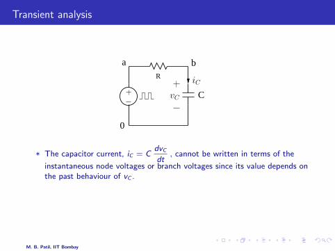
Transient analysis
aR
b
C
0
vC
iC
* The capacitor current, iC = CdvCdt
, cannot be written in terms of the
instantaneous node voltages or branch voltages since its value depends onthe past behaviour of vC .
* We need some way of approximating the derivative in terms of the pastbehaviour of vC .
M. B. Patil, IIT Bombay

Discretization of time
∆∆∆∆ t t t t
time
2 31 N−1
t t t t t tNN−1
t t end
. . . . . .
begin
2 30 1
* Discretization of time is required since numerical solution can only beobtained at a finite number of points.
* The time steps (∆ti ) may not be uniform.
* Generally, the time steps are computed dynamically, not a priori.
M. B. Patil, IIT Bombay

Discretization of time
Vs
R
C
0
V
(a) (b) (c) 0
2
4
6
8
10
0 5 10 15 20 25
V (
Vol
ts)
Time (sec)
0
2
4
6
8
10
0 5 10 15 20 25
V (
Vol
ts)
Time (sec)
0
2
4
6
8
10
0 5 10 15 20 25
V (
Vol
ts)
Time (sec)
(a) Typical simulator output.
(b) After connecting the output points with line segments.
(c) After removing the output points (but retaining the segments), thewaveform looks continuous, but this is an illusion!
M. B. Patil, IIT Bombay

Transient simulation: Forward Euler method
tn tn+1
x
t
h
xn
xn+1(predicted)
* Considerdx
dt= f (t, x). We have the solution at tn and want to
obtain x(tn+1).
* Compute the slope at tn:dx
dt
∣∣∣∣t=tn
= f (tn, xn).
*xn+1 − xntn+1 − tn
≈ f (tn, xn)
→ xn+1 = xn + h f (tn, xn).
M. B. Patil, IIT Bombay

Transient simulation: Forward Euler method
tn tn+1
x
t
h
xn
xn+1(predicted)
* Considerdx
dt= f (t, x). We have the solution at tn and want to
obtain x(tn+1).
* Compute the slope at tn:dx
dt
∣∣∣∣t=tn
= f (tn, xn).
*xn+1 − xntn+1 − tn
≈ f (tn, xn)
→ xn+1 = xn + h f (tn, xn).
M. B. Patil, IIT Bombay

Transient simulation: Forward Euler method
tn tn+1
x
t
h
xn
xn+1(predicted)
* Considerdx
dt= f (t, x). We have the solution at tn and want to
obtain x(tn+1).
* Compute the slope at tn:dx
dt
∣∣∣∣t=tn
= f (tn, xn).
*xn+1 − xntn+1 − tn
≈ f (tn, xn)
→ xn+1 = xn + h f (tn, xn).
M. B. Patil, IIT Bombay

Transient simulation: Forward Euler method
tn tn+1
x
t
h
xn
xn+1(predicted)
* Considerdx
dt= f (t, x). We have the solution at tn and want to
obtain x(tn+1).
* Compute the slope at tn:dx
dt
∣∣∣∣t=tn
= f (tn, xn).
*xn+1 − xntn+1 − tn
≈ f (tn, xn)
→ xn+1 = xn + h f (tn, xn).
M. B. Patil, IIT Bombay

Transient simulation: Forward Euler method
tn tn+1
x
t
h
xn
xn+1(predicted)
* Considerdx
dt= f (t, x). We have the solution at tn and want to
obtain x(tn+1).
* Compute the slope at tn:dx
dt
∣∣∣∣t=tn
= f (tn, xn).
*xn+1 − xntn+1 − tn
≈ f (tn, xn) → xn+1 = xn + h f (tn, xn).
M. B. Patil, IIT Bombay

Transient analysis: a quick look
tn tn+1
xn
xn+1
hx
t
Method Approximation fordx
dt= f (t, x)
Forward Eulerxn+1 − xn
h= f (tn, xn)
Backward Eulerxn+1 − xn
h= f (tn+1, xn+1)
Trapezoidalxn+1 − xn
h=
1
2[f (tn, xn) + f (tn+1, xn+1)]
M. B. Patil, IIT Bombay

Transient analysis: a quick look
tn tn+1
xn
xn+1
hx
t
Method Approximation fordx
dt= f (t, x)
Forward Eulerxn+1 − xn
h= f (tn, xn)
Backward Eulerxn+1 − xn
h= f (tn+1, xn+1)
Trapezoidalxn+1 − xn
h=
1
2[f (tn, xn) + f (tn+1, xn+1)]
M. B. Patil, IIT Bombay

Transient analysis: a quick look
tn tn+1
xn
xn+1
hx
t
Method Approximation fordx
dt= f (t, x)
Forward Eulerxn+1 − xn
h= f (tn, xn)
Backward Eulerxn+1 − xn
h= f (tn+1, xn+1)
Trapezoidalxn+1 − xn
h=
1
2[f (tn, xn) + f (tn+1, xn+1)]
M. B. Patil, IIT Bombay

Application to x =−x , with x(0) = 1
FE :xn+1 − xn
h= f (tn, xn) = −xn
BE :xn+1 − xn
h= f (tn+1, xn+1) = −xn+1
TRZ :xn+1 − xn
h=
1
2[f (tn, xn) + f (tn+1, xn+1)] = −1
2(xn + xn+1)
Simple manipulation yields the following approximations:
FE : xn+1 = xn (1− h)
BE : xn+1 = xn1
1 + h
TRZ : xn+1 = xn1− h/2
1 + h/2
M. B. Patil, IIT Bombay

Application to x =−x , with x(0) = 1
The exact solution is x(t) = e−t . Expanding around tn, we get,
xn+1 = xn + hdx
dt+ · · · = xn + h(−e−tn ) + · · · = xn(1− h + h2/2− h3/6 + · · · ) .
Compare with
FE : xn+1 = xn (1− h)
BE : xn+1 = xn1
1 + h= xn (1− h + h2 + · · · )
TRZ : xn+1 = xn1− h/2
1 + h/2= xn (1− h + h2/2− h3/4 + · · · )
* If h 1, the three approximations are equivalent, as we would expect.
* If the starting point x(tn) is the same, the “error” (difference between theexact and numerical solutions) is O(h2) for FE and BE, and O(h3) forTRZ.
M. B. Patil, IIT Bombay

Application to x =−x , with x(0) = 1
numerical
exact
10
10
10
100
−4
−8
−12
10−110−210−310−4 100
BE
TRZ
FE
step size (h)
ttn+1tn
ǫlocal
tn+2
x
ǫ local
* The local error is the error made in a single step, assuming that thestarting point is exact. In this case, starting from the exact value,x(0) = 1, the difference |x(h)− x(h)| has been computed.
* If h→ h/10, the error decreases by a factor of 102 for the FE and BEmethods, and by 103 for the TRZ method.
* The TRZ method is therefore said to be more accurate than FE or BE.
M. B. Patil, IIT Bombay

Application to x =−x , with x(0) = 1
x
t
h=0.5
0.0
0.2
0.4
0.6
0.8
1.0
0 1 2 3 4 5
BE
exact
TRZ
* The higher accuracy of the TRZ method allows larger time steps.
M. B. Patil, IIT Bombay

Application to x =−x , with x(0) = 1
x
t
h=0.5
0.0
0.2
0.4
0.6
0.8
1.0
0 1 2 3 4 5
BE
exact
TRZ
* The higher accuracy of the TRZ method allows larger time steps.
M. B. Patil, IIT Bombay

Comparison of FE and BE for x = −x , x(0) = 1
0.0
0.2
0.4
0.6
0.8
1.0
0 1 2 3 4
h=0.1
exactFEBE
M. B. Patil, IIT Bombay

Comparison of FE and BE for x = −x , x(0) = 1
0.0
0.2
0.4
0.6
0.8
1.0
0 1 2 3 4
h=0.1
exactFEBE
0.0
0.2
0.4
0.6
0.8
1.0
0 1 2 3 4
h=0.5
M. B. Patil, IIT Bombay

Comparison of FE and BE for x = −x , x(0) = 1
0.0
0.2
0.4
0.6
0.8
1.0
0 1 2 3 4
h=0.1
exactFEBE
0.0
0.2
0.4
0.6
0.8
1.0
0 1 2 3 4
h=0.5
−1
0
1
0 5 10 15 20
h=2.0
M. B. Patil, IIT Bombay

Comparison of FE and BE for x = −x , x(0) = 1
0.0
0.2
0.4
0.6
0.8
1.0
0 1 2 3 4
h=0.1
exactFEBE
0.0
0.2
0.4
0.6
0.8
1.0
0 1 2 3 4
h=0.5
−3
−2
−1
0
1
2
3
0 5 10 15 20
h=2.1
−1
0
1
0 5 10 15 20
h=2.0
M. B. Patil, IIT Bombay

Comparison of FE and BE for x = −x , x(0) = 1
* Although the FE and BE methods are comparable in accuracy, the FEmethod is unstable and therefore not useful for circuit simulation.
* Can we not use a smaller time step and avoid the instability problem?Yes, but it increases the simulation time, and in some cases (stiff circuits),by orders of magnitude!
* The issue of stability rules out many other methods as well.
M. B. Patil, IIT Bombay

Comparison of FE and BE for x = −x , x(0) = 1
* Although the FE and BE methods are comparable in accuracy, the FEmethod is unstable and therefore not useful for circuit simulation.
* Can we not use a smaller time step and avoid the instability problem?
Yes, but it increases the simulation time, and in some cases (stiff circuits),by orders of magnitude!
* The issue of stability rules out many other methods as well.
M. B. Patil, IIT Bombay

Comparison of FE and BE for x = −x , x(0) = 1
* Although the FE and BE methods are comparable in accuracy, the FEmethod is unstable and therefore not useful for circuit simulation.
* Can we not use a smaller time step and avoid the instability problem?Yes, but it increases the simulation time, and in some cases (stiff circuits),by orders of magnitude!
* The issue of stability rules out many other methods as well.
M. B. Patil, IIT Bombay

Comparison of FE and BE for x = −x , x(0) = 1
* Although the FE and BE methods are comparable in accuracy, the FEmethod is unstable and therefore not useful for circuit simulation.
* Can we not use a smaller time step and avoid the instability problem?Yes, but it increases the simulation time, and in some cases (stiff circuits),by orders of magnitude!
* The issue of stability rules out many other methods as well.
M. B. Patil, IIT Bombay

Explicit and implicit methods
Consider the ODE,
dx
dt= −x2, with 1 ≤ t ≤ 5, x(1) = 1 .
Application of the FE, BE, and TRZ formulas yields,
xn+1 = xn + h (−x2n ) (FE) ,
xn+1 = xn + h (−x2n+1) (BE) ,
xn+1 = xn +h
2(−x2
n − x2n+1) (TRZ) .
* In the FE formula, xn+1 can be explicitly evaluated in terms of xn.
* The BE and TRZ formulas result in equations which must be solved forxn+1. This is much more work, and it gets worse when there are manyequations involved.
* However, the FE method is not useful because it can be unstable in somecases.
M. B. Patil, IIT Bombay

Choice of method for transient simulation
* Two major concerns: accuracy (order) and stability
* A method with a higher accuracy (order) is more efficient as it allows alarger time step ⇒ fewer time points ⇒ faster simulation.
* However, high-order methods are conditionally stable, i.e., if the time stepis large (compared to the smallest time constant in the circuit), thesolution grows indefinitely, as in the FE example.
* Power electronic circuits are usually stiff (i.e., they involve time constantswhich are vastly different), and one cannot afford to make h smaller thanthe smallest τ because(a) such a high resolution is not required,(b) it would dramatically increase the simulation time.
* The stability constraints significantly reduce the choices available forcircuit simulation. BE, Gear (order 2), and Trapezoidal methods arecommonly used.
M. B. Patil, IIT Bombay

Equivalent circuit for a capacitor
With Backward Euler method, we get
vn+1C − vn
C
h=
1
Cin+1C .
i.e., vn+1C =
h
Cin+1C + vn
C OR in+1C =
C
hvn+1C − C
hvnC .
+
iC
vC
vnC C/h
in+1C
h/C
vnC
vn+1C
h/C
in+1C
M. B. Patil, IIT Bombay

Equivalent circuit for a capacitor
With Backward Euler method, we get
vn+1C − vn
C
h=
1
Cin+1C .
i.e., vn+1C =
h
Cin+1C + vn
C OR in+1C =
C
hvn+1C − C
hvnC .
+
iC
vC
vnC C/h
in+1C
h/C
vnC
vn+1C
h/C
in+1C
M. B. Patil, IIT Bombay

Time step selection
* In some circuits, a constant ∆t is appropriate; in others, especially withmany switching events, automatic time step selection is more effective.
* Automatic time step selection is based on (a) estimate of the localtruncation error at a given time step, (b) convergence behaviour of N-Riterations.
* Power electronic circuits are generally nonlinear; time step has asignificant impact on convergence of N-R iterations. Option (b) istherefore very effective.
* N-R convergence
- The solution obtained at ti serves as the “initial guess” at ti+1.- ∆t too large ⇒ N-R iterations may not converge.- ∆t too small ⇒ large simulation time.
M. B. Patil, IIT Bombay

Time step selection
* In some circuits, a constant ∆t is appropriate; in others, especially withmany switching events, automatic time step selection is more effective.
* Automatic time step selection is based on (a) estimate of the localtruncation error at a given time step, (b) convergence behaviour of N-Riterations.
* Power electronic circuits are generally nonlinear; time step has asignificant impact on convergence of N-R iterations. Option (b) istherefore very effective.
* N-R convergence
- The solution obtained at ti serves as the “initial guess” at ti+1.
- ∆t too large ⇒ N-R iterations may not converge.- ∆t too small ⇒ large simulation time.
M. B. Patil, IIT Bombay

Time step selection
* In some circuits, a constant ∆t is appropriate; in others, especially withmany switching events, automatic time step selection is more effective.
* Automatic time step selection is based on (a) estimate of the localtruncation error at a given time step, (b) convergence behaviour of N-Riterations.
* Power electronic circuits are generally nonlinear; time step has asignificant impact on convergence of N-R iterations. Option (b) istherefore very effective.
* N-R convergence
- The solution obtained at ti serves as the “initial guess” at ti+1.- ∆t too large ⇒ N-R iterations may not converge.
- ∆t too small ⇒ large simulation time.
M. B. Patil, IIT Bombay

Time step selection
* In some circuits, a constant ∆t is appropriate; in others, especially withmany switching events, automatic time step selection is more effective.
* Automatic time step selection is based on (a) estimate of the localtruncation error at a given time step, (b) convergence behaviour of N-Riterations.
* Power electronic circuits are generally nonlinear; time step has asignificant impact on convergence of N-R iterations. Option (b) istherefore very effective.
* N-R convergence
- The solution obtained at ti serves as the “initial guess” at ti+1.- ∆t too large ⇒ N-R iterations may not converge.- ∆t too small ⇒ large simulation time.
M. B. Patil, IIT Bombay

Automatic time step selection
Yes No
Yes
Stop
N−R
No
Yes
No
Converged?
Start (∆t = ∆t0)
∆t = ∆t/k2
∆t = k1∆t
∆t = ∆tmax ? ∆t = ∆tmin ?
t = t+∆t
M. B. Patil, IIT Bombay

Automatic time step selection: example
V2
V4
V1
Vs
V2
R2
42
0
C
R1 R
C
0
0
VV4
3
µ
Automatic time step selectionbased on convergence of N−Riterations
0
1
2
3
4
5
V , V
(V
olt
s)
0
20
40
60
80
100
120
2 3 4 5 6
time (msec)
h (
s
ec)
M. B. Patil, IIT Bombay

Transient simulation: are the results accurate?
* very difficult to judge except for simple problems
* In practice, reduce ∆t by a factor of 2 and see if the results are different.
* Usually, the user would have some idea of the time scale, For example,(a) Buck converter: ∆t = Tc/50 may be appropriate.(b) Half-wave rectifier: ∆t = T/50 may be appropriate.Such a rule of thumb provides a good starting point.
M. B. Patil, IIT Bombay

Steady-State Waveform (SSW) Analysis
* In many periodic systems, only the steady-state behaviour is of interest(and not how it is attained). e.g., power electronic circuits, rf circuits
* Transient simulation (from some initial condition to the steady state) mayinvolve thousands of cycles; this is very expensive.
* Total time for which transient simulation needs to be performed to reachthe steady state is not known a priori; need to rely on a trial-and-errorapproach.
* It is much faster to obtain the steady-state information directly where anonlinear problem in the state variables is solved.
M. B. Patil, IIT Bombay

SSW Analysis: Buck Converter
0
+
a b c
C V
i
R
L
20.48
20.44
0.026 0.028 0.030
V (V
olts
)
Time (sec)
0
20
40
0 0.01 0.02 0.03
V (V
olts
)
Time (sec)
* A large number of cycles are required if transient simulation is used.(Note that, for this example, the steady state is not quite reached asindicated by the small amplitude variation.)
* If a component value (L or C) is changed, we would not know how longto simulate to attain steady state. This is cumbersome.
M. B. Patil, IIT Bombay

SSW Analysis: Basic idea
V c
Vs
R1
R2
0
C D
ab
c
−0.4
−0.2
0
0.2
0.4
0 0.01 0.02time
* Start with an initial guess for the state variable(s) (the capacitor voltagehere).
* Integrate for one cycle. Is Vc(T ) =Vc(0)?
* If yes (red curve), we have obtained the SSW solution; if not, we need tocompute a better initial guess (in an outer Newton-Raphson loop) andrepeat [7].
M. B. Patil, IIT Bombay

SSW: Examples
Example Ntrns Nssw
Buck Converter 750 4
Boost Converter 625 3
Cuk Converter 1250 3
1-φ half-wave rectifier 150 3
1-φ half-controlled bridge converter 110 4
3-φ diode bridge rectifier 200 4
Induction motor 125 17
* Note the dramatic reduction in computational effort for the SSW methodas compared to transient analysis.
M. B. Patil, IIT Bombay

References
[1] L. O. Chua and P. M. Lin, Computer-Aided Analysis of Electronic Circuits, Englewood Cliffs:Prentice-Hall, 1976.
[2] W. J. McCalla, Fundamentals of Computer-Aided Circuit Simulation, Boston: KluwerAcademic Publishers, 1987.
[3] R. Raghuram, Computer Simulation of Electronic Circuits, New Delhi: Wiley Eastern, 1989.
[4] K. S. Kundert, The Designer’s Guide to SPICE and SPECTRE, Boston: Kluwer AcademicPublishers, 1995.
[5] M. B. Patil, V. Ramanarayanan, and V. T. Ranganathan, Simulation of Power ElectronicCircuits, to be published.
[6] C. D. Hachtel and R. K. Brayton and F. G. Gustavson, “The sparse tableau approach tonetwork analysis and design,” IEEE Trans. CT, vol. 18, pp. 101-113, 1971.
[7] F. R. Colon and T. N. Trick, “Fast periodic steady-state analysis for large-signal electroniccircuits,” IEEE J. Solid-State Circuits, vol. 8, pp. 260-269, 1973.
[8] C. F. Gerald and P. O. Whitley, Applied Numerical Analysis, Delhi: Pearson Education India,1999.
M. B. Patil, IIT Bombay