Analog Circuit Simulation with TINA-TI · 2013-12-04 · , TINA-TI, Texas Instruments, DesignSoft, Circuit Simulation, Analog Simulation Tool, Circuit Analysis Introduction TINA TM

1 | P a g eKyle Christian Team #7

Analog Circuit Simulation

with TINA-TI

ECE 480

Application Note

Kyle Christian

Team #7

November 4th, 2013


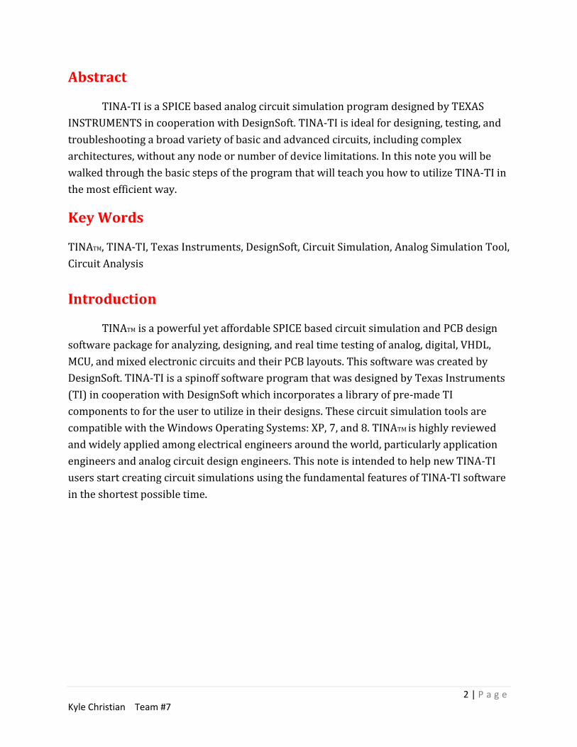
Abstract

TINA-TI is a SPICE based analog circuit simulation program designed by TEXAS

INSTRUMENTS in cooperation with DesignSoft. TINA-TI is ideal for designing, testing, and

troubleshooting a broad variety of basic and advanced circuits, including complex

architectures, without any node or number of device limitations. In this note you will be

walked through the basic steps of the program that will teach you how to utilize TINA-TI in

the most efficient way.

Key Words

TINATM, TINA-TI, Texas Instruments, DesignSoft, Circuit Simulation, Analog Simulation Tool,

Circuit Analysis

Introduction

TINATM is a powerful yet affordable SPICE based circuit simulation and PCB design

software package for analyzing, designing, and real time testing of analog, digital, VHDL,

MCU, and mixed electronic circuits and their PCB layouts. This software was created by

DesignSoft. TINA-TI is a spinoff software program that was designed by Texas Instruments

(TI) in cooperation with DesignSoft which incorporates a library of pre-made TI

components to for the user to utilize in their designs. These circuit simulation tools are

compatible with the Windows Operating Systems: XP, 7, and 8. TINATM is highly reviewed

and widely applied among electrical engineers around the world, particularly application

engineers and analog circuit design engineers. This note is intended to help new TINA-TI

users start creating circuit simulations using the fundamental features of TINA-TI software

in the shortest possible time.


Table of Contents

Getting Started…………………………………………………………………………………………………………4

Schematic Editing…………………………………………………………………………………………………….5

Overview……………………………………………………………………………………………………….5

Adding Components………………………………………………………………………………………6

Schematic Wiring & Connections…………………………………………………………………..9

Analysis & Simulation……………………………………………………………………………………………...11

Running ERC………………………………………………………………………………………………….11

Setting Mode & DC Analysis…………………………………………………………………………..12

Transient Analysis………………………………………………………………………………………...15

Visual Testing & Measurements………………………………………………………………………………16

Appendix…………………………………………………………………………………………………………………17

References………………………………………………………………………………………………………………17


Part A: Getting Started

To begin, use this link (http://www.ti.com/tool/tina-ti) which will take you to TI’s

website. Once you have arrived at the site you will be able to download the TINA-TI

simulation software as seen in Figure 1 below. This software is free to download, and is

available in multiple languages.

(Figure 1)- Available TINA-TI downloads

As mentioned earlier TINA-TI is available for Microsoft Windows XP, 7, or 8. If you are

using a Mac operating system, you can either run it under a Windows emulator or virtual

machines. You can find a free version of the emulator at the following website

(http://www.parallels.com/download/). Once you have selected which TINA-TI version you

would like to use, click Register/Download button to begin the download to your computer.

Keep in mind the hardware requirements if the program cannot be correctly installed.

The hardware requirements are listed below:

64MB of RAM

Pentium processor

Hard drive with at least 100MB

http://www.ti.com/tool/tina-ti

http://www.parallels.com/download/


Part B: Schematic Editing

B.1-Overview

Once the program is finished installing on your computer, there should be a new

icon on your desktop labeled “Tina-TI” as shown below in Figure 2.

(Figure 2)- Desktop Icon

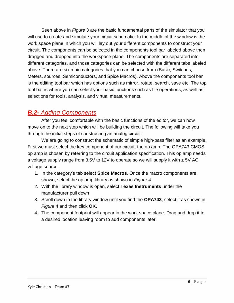
Click the icon to start the program, the schematic editor window will open up as shown

below in Figure 3.

(Figure 3)- Schematic Editor Window


Seen above in Figure 3 are the basic fundamental parts of the simulator that you

will use to create and simulate your circuit schematic. In the middle of the window is the

work space plane in which you will lay out your different components to construct your

circuit. The components can be selected in the components tool bar labeled above then

dragged and dropped into the workspace plane. The components are separated into

different categories, and those categories can be selected with the different tabs labeled

above. There are six main categories that you can choose from (Basic, Switches,

Meters, sources, Semiconductors, and Spice Macros). Above the components tool bar

is the editing tool bar which has options such as mirror, rotate, search, save etc. The top

tool bar is where you can select your basic functions such as file operations, as well as

selections for tools, analysis, and virtual measurements.

B.2- Adding Components

After you feel comfortable with the basic functions of the editor, we can now

move on to the next step which will be building the circuit. The following will take you

through the initial steps of constructing an analog circuit.

We are going to construct the schematic of simple high-pass filter as an example.

First we must select the key component of our circuit, the op amp. The OPA743 CMOS

op amp is chosen by referring to the circuit application specification. This op amp needs

a voltage supply range from 3.5V to 12V to operate so we will supply it with ± 5V AC

voltage source.

1. In the category’s tab select Spice Macros. Once the macro components are

shown, select the op amp library as shown in Figure 4.

2. With the library window is open, select Texas Instruments under the

manufacturer pull down

3. Scroll down in the library window until you find the OPA743, select it as shown in

Figure 4 and then click OK.

4. The component footprint will appear in the work space plane. Drag and drop it to

a desired location leaving room to add components later.


(Figure 4)- Selecting Op Amp (active comp.)

Components are easy to select from different categories as illustrated in the

previous section. These categories contain many passive and active components. Left

clicking on a schematic symbol for a particular component selects it. Once selected,

drag the component into a position, placing it so there is a decent amount of space

between it and other components. Then left click again to place it. Continuing with the

construction of our circuit schematic, let’s add a 15kΩ resistor which will be connected

to the (-) leg of the op amp.


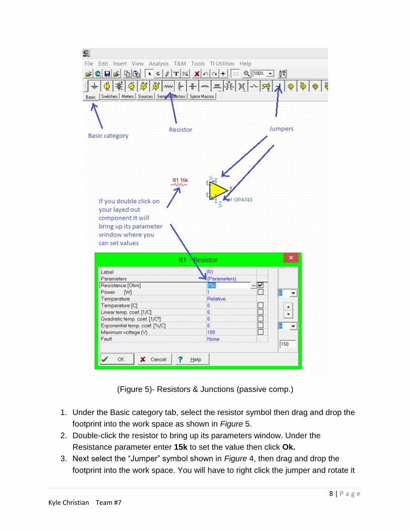
(Figure 5)- Resistors & Junctions (passive comp.)

1. Under the Basic category tab, select the resistor symbol then drag and drop the

footprint into the work space as shown in Figure 5.

2. Double-click the resistor to bring up its parameters window. Under the

Resistance parameter enter 15k to set the value then click Ok.

3. Next select the “Jumper” symbol shown in Figure 4, then drag and drop the

footprint into the work space. You will have to right click the jumper and rotate it


to make it symmetrical to fit on the V+ terminal. Once rotated drag and drop the

jumper so that the connection end is on the V+ terminal. Repeat this for the V-

terminal. Jumpers will be explained in the next section.

4. Continue to drag and drop the rest of the components needed for the high-pass

filter

B.3- Schematic Wiring and Connection

Once you have placed all of the needed components for the high-pass filter into

your work space plane, the next step is to arrange them in a position so that you have a

clean schematic and then wire the different nodes together. Each component has

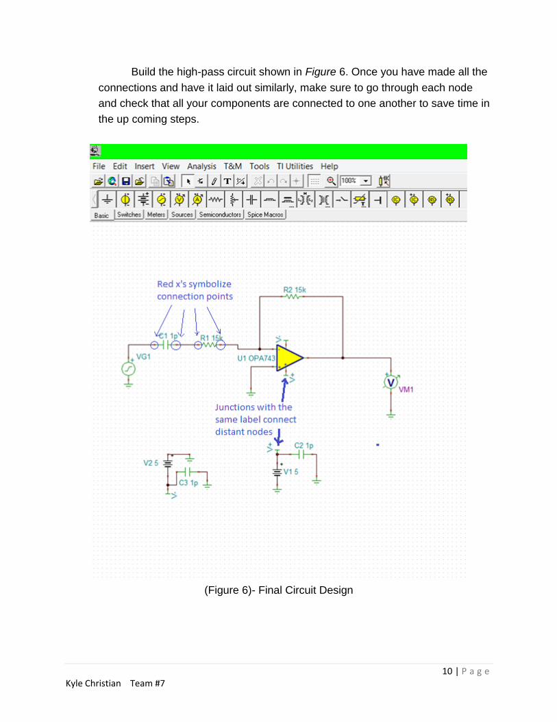
connection node/s which are marked by the red “x’s” as seen in Figure 6. The process

is very simple to wire one node to another. Simply place your cursor over the

connection node of the component you wish to wire, your cursor will change to a pencil

symbol. Once this happens left click and a wire trace will follow your cursor wherever

you drag it. Take the wire to the connecting component and it should ‘snap’ to the node.

When arranging and wiring your circuit, a good tip to keep in mind is to give yourself

enough room between components to make clear and easy connections. Below are

some more important tips to help you avoid make errors in your circuit layout.

1. Some components have such as voltage sources, and voltage generators shown

in Figure 6 have their polarity marked by a (+) symbol. Make sure your

components are directions are correct to the circuit design to save time before

you proceed. (Adjust direction by right clicking and select Rotate/Mirror)

2. When making parallel connections (wire-to-wire) TINA-TI confirms connection

points with a “black dot”. An example of this can be seen in Figure 6 between R2

and the output of the OPA743.

3. If your circuit is very complex, clustered, or busy a good tool to use is the

“Junction” components that we added earlier. Junctions are used to connect

distant nodes to one another. Our high-pas filter is a very simple design and is

just being used for reference but junctions are very helpful if you want to

separate phases of a circuit or, distribute one power supply over many areas of a

circuit instead of having multiple ones, or just if you want to give your schematic

a lean look like we did here. Junctions with the same label will connect to one

another as demonstrated in Figure 6.

4. Finally Label your components to your desired liking so you can identify them

easier.


Build the high-pass circuit shown in Figure 6. Once you have made all the

connections and have it laid out similarly, make sure to go through each node

and check that all your components are connected to one another to save time in

the up coming steps.

(Figure 6)- Final Circuit Design


Part C: Analysis & Simulation

C.1- Running ERC

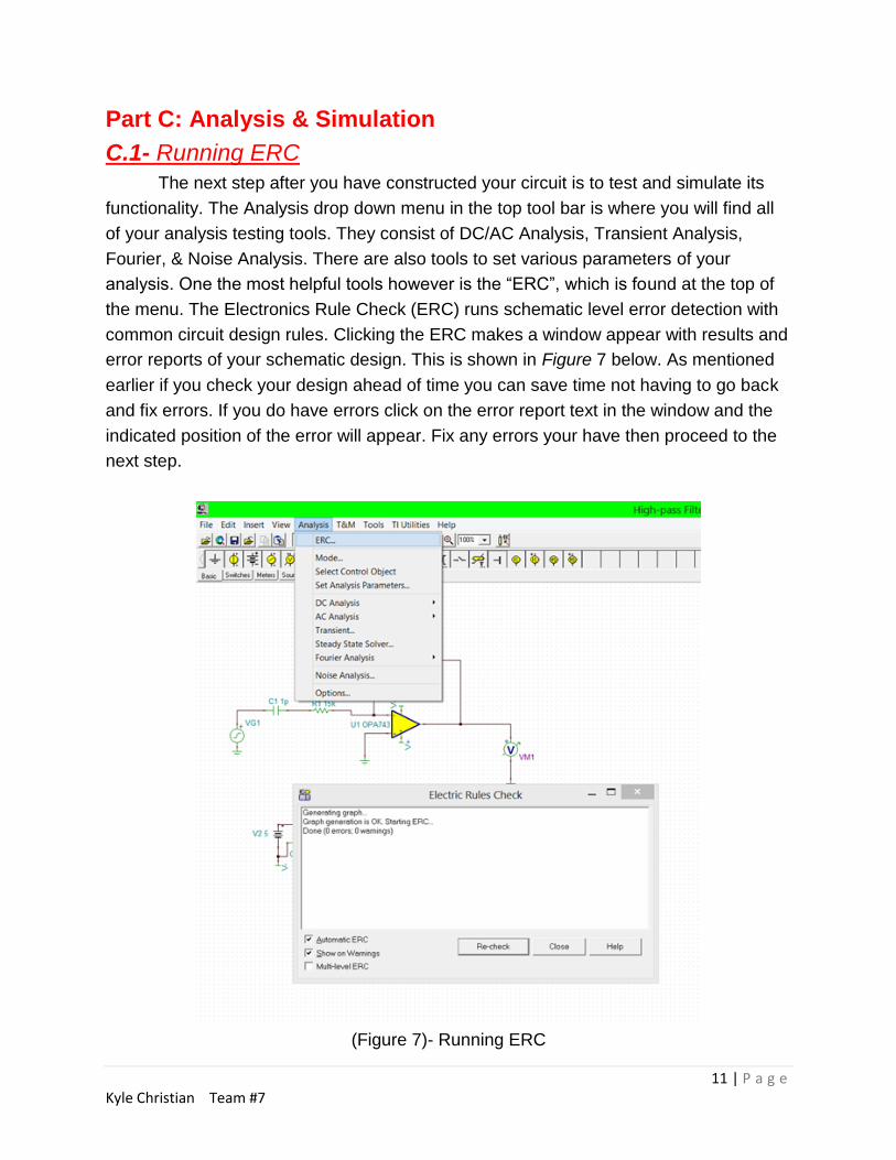
The next step after you have constructed your circuit is to test and simulate its

functionality. The Analysis drop down menu in the top tool bar is where you will find all

of your analysis testing tools. They consist of DC/AC Analysis, Transient Analysis,

Fourier, & Noise Analysis. There are also tools to set various parameters of your

analysis. One the most helpful tools however is the “ERC”, which is found at the top of

the menu. The Electronics Rule Check (ERC) runs schematic level error detection with

common circuit design rules. Clicking the ERC makes a window appear with results and

error reports of your schematic design. This is shown in Figure 7 below. As mentioned

earlier if you check your design ahead of time you can save time not having to go back

and fix errors. If you do have errors click on the error report text in the window and the

indicated position of the error will appear. Fix any errors your have then proceed to the

next step.

(Figure 7)- Running ERC


C.2- Setting Mode & DC Analysis

The first analysis performed on a circuit is generally a DC analysis. This test provides a

reality check so that normal dc operating conditions can be verified. The DC Analysis

function in the analysis pull down tab has a selection of sub-functions which consist of

Calculate Nodal Voltages, Table of DC results, DC Transfer Characteristic, and

Temperature Analysis.

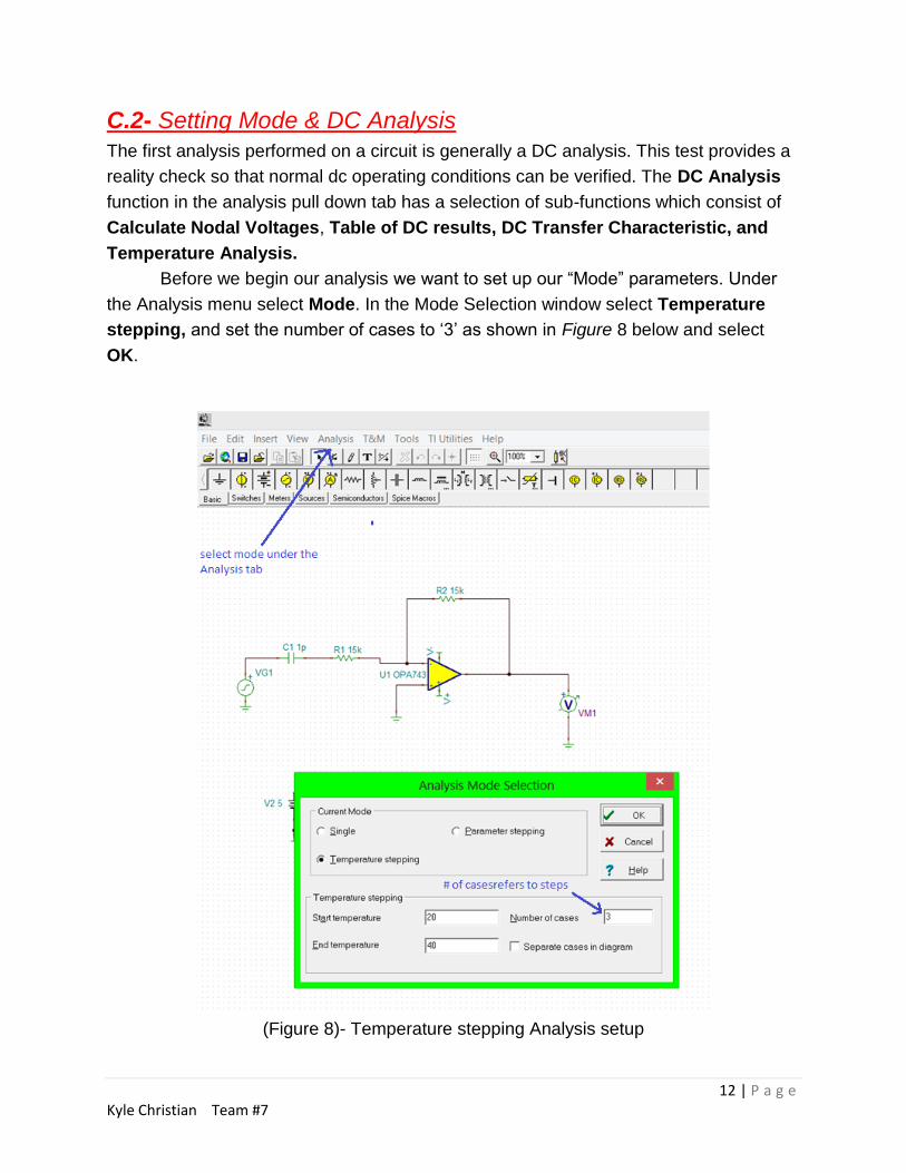
Before we begin our analysis we want to set up our “Mode” parameters. Under

the Analysis menu select Mode. In the Mode Selection window select Temperature

stepping, and set the number of cases to ‘3’ as shown in Figure 8 below and select

OK.

(Figure 8)- Temperature stepping Analysis setup


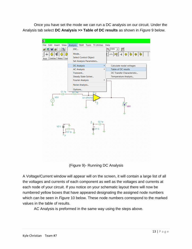
Once you have set the mode we can run a DC analysis on our circuit. Under the

Analysis tab select DC Analysis >> Table of DC results as shown in Figure 9 below.

(Figure 9)- Running DC Analysis

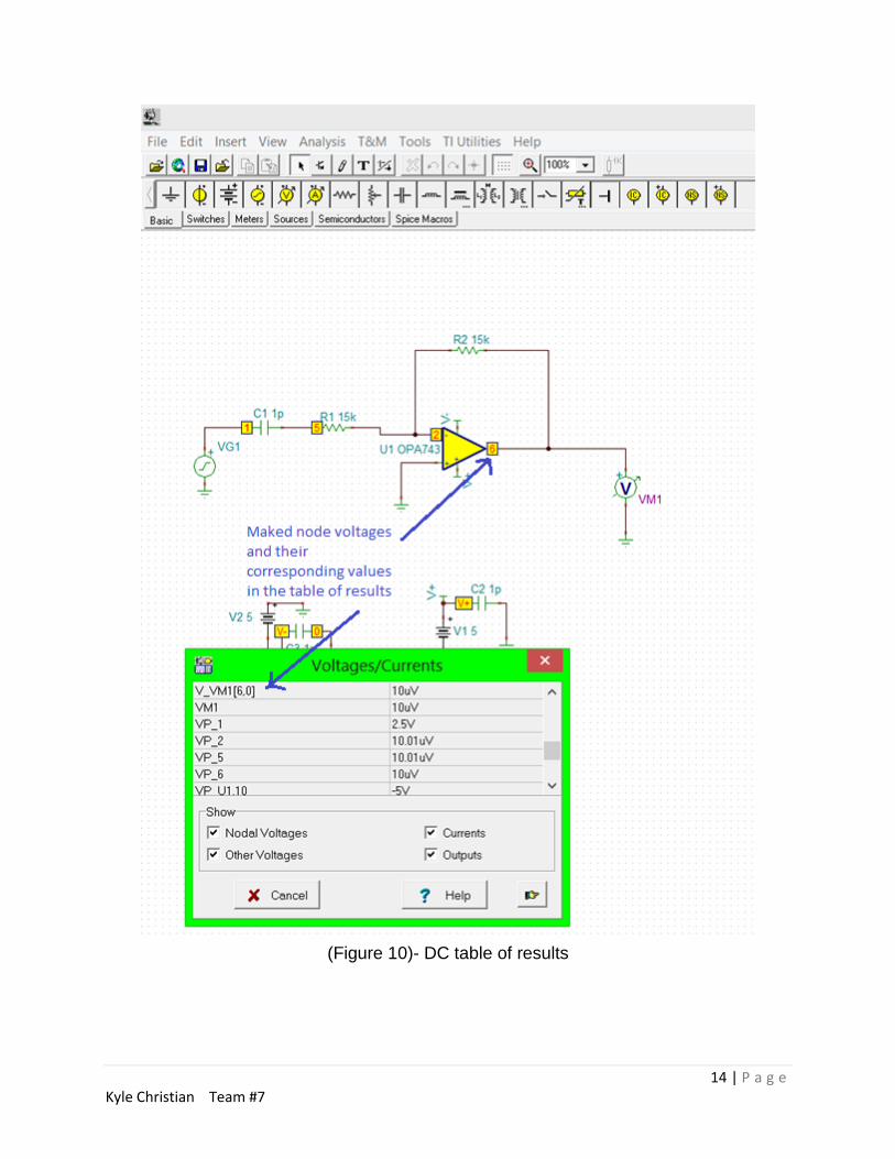
A Voltage/Current window will appear will on the screen, it will contain a large list of all

the voltages and currents of each component as well as the voltages and currents at

each node of your circuit. If you notice on your schematic layout there will now be

numbered yellow boxes that have appeared designating the assigned node numbers

which can be seen in Figure 10 below. These node numbers correspond to the marked

values in the table of results.

AC Analysis is preformed in the same way using the steps above.


(Figure 10)- DC table of results


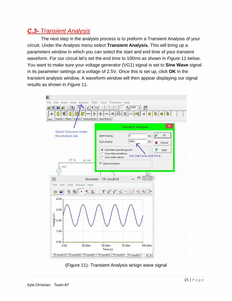
C.3- Transient Analysis

The next step in the analysis process is to preform a Transient Analysis of your

circuit. Under the Analysis menu select Transient Analysis. This will bring up a

parameters window in which you can select the start and end time of your transient

waveform. For our circuit let’s set the end time to 100ms as shown in Figure 11 below.

You want to make sure your voltage generator (VG1) signal is set to Sine Wave signal

in its parameter settings at a voltage of 2.5V. Once this is set up, click OK in the

transient analysis window. A waveform window will then appear displaying our signal

results as shown in Figure 11.

(Figure 11)- Transient Analysis w/sign wave signal


The outputted plot shows the expected signal that we were looking for from our

High-pass Filter design. Further functions and results can be obtained from the plot

window such as altering color, editing labels, adding text, and scaling.

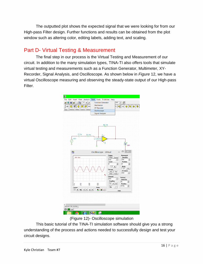
Part D- Virtual Testing & Measurement

The final step in our process is the Virtual Testing and Measurement of our

circuit. In addition to the many simulation types, TINA-TI also offers tools that simulate

virtual testing and measurements such as a Function Generator, Multimeter, XY-

Recorder, Signal Analysis, and Oscilloscope. As shown below in Figure 12, we have a

virtual Oscilloscope measuring and observing the steady-state output of our High-pass

Filter.

(Figure 12)- Oscilloscope simulation

This basic tutorial of the TINA-TI simulation software should give you a strong

understanding of the process and actions needed to successfully design and test your

circuit designs.


Appendix

TINA-TI Application FAQ’s

(http://www.ti.com/analog/docs/gencontent.tsp?familyId=02&genContentId=33361)

References

TINA-TI download link

(http://www.ti.com/tool/tina-ti)

Windows emulator for MAC’s link

(http://www.parallels.com/download/)

http://www.ti.com/analog/docs/gencontent.tsp?familyId=02&genContentId=33361

http://www.ti.com/tool/tina-ti

http://www.parallels.com/download/

Documents

Analog Circuit Simulation with TINA-TI · 2013-12-04 · , TINA-TI, Texas Instruments, DesignSoft, Circuit Simulation, Analog Simulation Tool, Circuit Analysis Introduction TINA TM