Embed Size (px)
Citation preview

Cloud-aided collaborative estimation by ADMM-RLSalgorithms for connected vehicle prognostics
Technical Report TR-2017-01
Valentina Breschi∗, Ilya Kolmanovsky†, Alberto Bemporad∗
September 26, 2017
Abstract
As the connectivity of consumer devices is rapidly growing and cloudcomputing technologies are becoming more widespread, cloud-aided tech-niques for parameter estimation can be designed to exploit the theoreti-cally unlimited storage memory and computational power of the “cloud”,while relying on information provided by multiple sources.With the ultimate goal of developing monitoring and diagnostic strate-gies, this report focuses on the design of a Recursive Least-Squares (RLS)based estimator for identification over a group of devices connected to the“cloud”. The proposed approach, that relies on Node-to-Cloud-to-Node(N2C2N) transmissions, is designed so that: (i) estimates of the unknownparameters are computed locally and (ii) the local estimates are refinedon the cloud. The proposed approach requires minimal changes to local(pre-existing) RLS estimators.
1 Introduction
With the increasing connectivity between devices, the interest in distributed so-lutions for estimation [13], control [5] and machine learning [4] has been rapidlygrowing. In particular, the problem of parameter estimation over networks hasbeen extensively studied, especially in the context of Wireless Sensor Networks(WSNs). The methods designed to solve this identification problem can be di-vided into three groups: incremental approaches [10], diffusion approaches [3]and consensus-based distributed strategies [11]. Due to the low communica-tion power of the nodes in WSNs, research has mainly been devoted to obtainfully distributed approaches, i.e. methods that allow exchanges of informationbetween neighbor nodes only. Even though such a choice enables to reducemulti-hop transmissions and improve robustness to node failures, these strate-gies allows only neighbor nodes to communicate and thus to reach consensus.
The results in the report have been partially presented in a paper submitted to ACC 2018.
∗Valentina Breschi and Alberto Bemporad are with the IMT School for Advanced StudiesLucca, Piazza San Francesco 19, 55100 Lucca, Italy. [email protected];[email protected]†Ilya Kolmanovsky is with the Department of Aerospace Engineering, University of Michi-
gan, Ann Arbor, MI 48109, USA. [email protected]
1
arX
iv:1
709.
0797
2v1
[cs
.SY
] 2
2 Se
p 20
17

Communication Layer
Collect informationBroadcast
Global Updates
Global UpdatesCLOUD
Local Updates
· · · · · ·· · · · · ·
Figure 1: Cloud-connected vehicles.
As a consequence, to attain consensus on the overall network, its topology hasto be chosen to enable exchanges of information between the different groups ofneighbor nodes.At the same time, with recent advances in cloud computing [12] it has nowbecome possible to acquire and release resources with minimum effort so thateach node can have on-demand access to shared resources, theoretically charac-terized by unlimited storage space and computational power. This motivates toreconsider the approach towards a more centralized strategy where some com-putations are performed at the node level, while the most time and memoryconsuming ones are executed “on the cloud”. This requires the communicationbetween the nodes and a fusion center, i.e. the “cloud”, where the data gatheredfrom the nodes are properly merged.Cloud computing has been considered for automotive vehicle applications in [7]-[8] and [14]. As motivating example for another possible automotive application,consider a vehicle fleet with vehicles connected to the “cloud” (see Figure 1).In such a setting, measurements taken on-board of the vehicles can be used forcloud-based diagnostics and prognostics purposes. In particular, the measure-ments can be used to estimate parameters that may be common to all vehicles,such as parameters in components wear models or fuel consumption models, andparameters that may be specific to individual vehicles. References [15] and [6]suggest potential applications of such approaches for prognostics of automotivefuel pumps and brake pads. Specifically, the component wear rate as a functionof the workload (cumulative fuel flow or energy dissipated in the brakes) can becommon to all vehicles or at least to all vehicles in the same class.A related distributed diagnostic technique has been proposed in [1]. However itrelies on a fully-distributed scheme, introduced to reduce long distance trans-missions and to avoid the presence of a “critic” node in the network, i.e. a nodewhose failure causes the entire diagnostic strategy to fail.
2
In this report a centralized approach for recursive estimation of parametersin the least-squares sense is presented. The method has been designed underthe hypothesis of (i) ideal transmission, i.e. the information exchanged betweenthe cloud and the nodes is not corrupted by noise, and the assumption that (ii)all the nodes are described by the same model, which is supposed to be knowna priori. Differently from what is done in many distributed estimation meth-ods (e.g. see [11]), where the nodes estimate common unknown parameters, thestrategy we propose allows to account for more general consensus constraint. Asa consequence, for example, the method can be applied to problems where onlya subset of the unknowns is common to all the nodes, while other parametersare purely local, i.e. they are different for each node.Our estimation approach is based on defining a separable optimization problemwhich is then solved through the Alternating Direction Method of Multipliers(ADMM), similarly to what has been done in [11] but in a somewhat differentsetting. As shown in [11], the use of ADMM leads to the introduction of twotime scales based on which the computations have to be performed. In partic-ular, the local time scale is determined by the nodes’ clocks, while the cloudtime scale depends on the characteristics of the resources available in the centerof fusion and on the selected stopping criteria, used to terminate the ADMMiterations.The estimation problem is thus solved through a two-step strategy. In particu-lar: (i) local estimates are recursively retrieved by each node using the measure-ments acquired from the sensors available locally; (ii) global computations areperformed to refine the local estimates, which are supposed to be transmitted tothe cloud by each node. Note that, based on the aforementioned characteristics,back and forth transmissions to the cloud are required. A transmission schemereferred to as Node-to-Cloud-to-Node (N2C2N) is thus employed.The main features of the proposed strategies are: (i) the use of recursive formu-las to update the local estimates of the unknown parameters; (ii) the possibilityto account for the presence of both purely local and global parameters, that canbe estimated in parallel; (iii) the straightforward integration of the proposedtechniques with pre-existing Recursive Least-Squares (RLS) estimators alreadyrunning on board of the nodes.
The report is organized as follows. In Section 2 ADMM is introduced, whilein Section 3 is devoted to the statement of the considered problem. The ap-proach for collaborative estimation with full consensus is presented in Section 4,along with the results of simulation examples that show the effectiveness of theapproach and its performance in different scenarios. In Section 5 and Section 6the methods for collaborative estimation with partial consensus and for con-strained collaborative estimation with partial consensus are described, respec-tively. Results of simulation examples are also reported. Concluding remarksand directions for future research are summarized in Section 7.
1.1 Notation
Let Rn be the set of real vectors of dimension n and R+ be the set of positivereal number, excluding zero. Given a set A, let A be the complement of A.Given a vector a ∈ Rn, ‖a‖2 is the Euclidean norm of a. Given a matrix
3

A ∈ Rn×p, A′ denotes the transpose of A. Given a set A, let PA denote theEuclidean projection onto A. Let In be the identity matrix of size n and 0n bean n-dimensional column vector of ones.
2 Alternating Direction Method of Multipliers
The Alternating Direction Method of Multipliers (ADMM) [2] is an algorithmtailored for problems in the form
minimize f(θ)+
subject to Aθ +Bz = c,(1)
where θ ∈ Rnθ , z ∈ Rnz , f : Rnθ → R ∪ {+∞} and g : Rnz → R ∪ {+∞} areclosed, proper, convex functions and A ∈ Rp×nθ , B ∈ Rp×nz , c ∈ Rp.
To solve Problem (1), the ADMM iterations to be performed are
θ(k+1) = argminθ
L(θ, z(k), δ(k)), (2)
z(k+1) = argminz
L(θ(k+1), z, δ(k)), (3)
δ(k+1) = δ(k) + ρ(Aθ(k+1) +Bz(k+1) − c), (4)
where k ∈ N indicates the ADMM iteration, L is the augmented Lagrangianassociated to (1), i.e.
L(θ, z, δ) = f(θ) + g(z) + δ′ (Aθ +Bz − c) +ρ
2‖Aθ +Bz − c‖22 , (5)
δ ∈ Rp is the Lagrange multiplier and ρ ∈ R+ is a tunable parameter (see [2]for possible tuning strategies). Iterations (2)-(4) have to be run until a stoppingcriteria is satisfied, e.g. the maximum number of iterations is attained.
It has to be remarked that the convergence of ADMM to high accuracyresults might be slow (see [2] and references therein). However, the resultsobtained with a few tens of iterations are usually accurate enough for most ofapplications. For further details, the reader is referred to [2].
2.1 ADMM for constrained convex optimization
Suppose that the problem to be addressed is
minθ
f(θ)
s.t. θ ∈ C,(6)
with θ ∈ Rnθ , f : Rnθ → R∪{+∞} being a closed, proper, convex function andC being a convex set, representing constraints on the parameter value.As explained in [2], (6) can be recast in the same form as (1) through theintroduction of the auxiliary variable z ∈ Rnθ and the indicator function of setC, i.e.
g(z) =
{0 if z ∈ C+∞ otherwise
. (7)
4

In particular, (6) can be equivalently stated as
minθ,z
f(θ) + g(z)
s.t. θ − z = 0.(8)
Then, the ADMM scheme to solve (8) is
θ(k+1) = argminθ
L(θ, z(k), δ(k)), (9)
z(k+1) = PC(θ(k+1) + δ(k)), (10)
δ(k+1) = δ(k) + ρ(θ(k+1) − z(k+1)) (11)
with L equal to
L(θ, z, δ) = f(θ) + g(z) + δ′(θ − z) +ρ
2‖θ − z‖22
2.2 ADMM for consensus problems
Consider the optimization problem given by
minθg
N∑n=1
fn(θg), (12)
where θg ∈ Rnθ and each term of the objective, i.e. fn : Rnθ → R ∪ {+∞}, is aproper, closed, convex function.Suppose that N processors are available to solve (12) and that, consequently,we are not interested in a centralized solution of the consensus problem. Asexplained in [2], ADMM can be used to reformulate the problem so that eachterm of the cost function in (12) is handled by its own.In particular, (12) can be reformulated as
minimize
N∑n=1
fn(θn)
subject to θn − θg = 0 n = 1, . . . , N.
(13)
Note that, thanks to the introduction of the consensus constraint, the costfunction in (13) is now separable.The augmented Lagrangian correspondent to (13) is given by
L({θn}Nn=1, θg, {δn}Nn=1) =
N∑n=1
(fn(θn) + δ′n(θn − θg) +
ρ
2‖θn − θg‖22
), (14)
and the ADMM iterations are
θ(k+1)n = argmin
θn
Ln(θn, δ(k)n , θg,(k)), n = 1, . . . , N (15)
θg,(k+1) =1
N
N∑n=1
(θ(k+1)n +
1
ρδ(k)n
), (16)
δ(k+1)n = δ(k)n + ρ
(θ(k+1)n − θg,(k+1)
), n = 1, . . . , N (17)
5

withLn = fn(θn) + (δn)′(θn − θg) +
ρ
2‖θn − θg‖22.
Note that, on the one hand (15) and (17) can be carried out independently byeach agent n ∈ {1, . . . , N}, (16) depends on all the updated local estimates.The global estimate should thus be updated in a “fusion center”, where all thelocal estimates are collected and merged.
3 Problem statement
Assume that (i) measurements acquired by N agents are available and that(ii) the behavior of the N data-generating systems is described by the sameknown model. Suppose that some parameters of the model, θn ∈ Rnθ withn = 1, . . . , N , are unknown and that their value has to to be retrieved fromdata. As the agents share the same model, it is also legitimate to assume that(iii) there exist a set of parameters θg ∈ Rng , with ng ≤ nθ, common to all theagents.
We aim at (i) retrieving local estimates of {θn}Nn=1, employing informationavailable at the local level only, and (ii) identifying the global parameter θg atthe “cloud” level, using the data collected from all the available sources. Toaccomplish these tasks (i) N local processors and (ii) and a “cloud”, where thedata are merged are needed.
The considered estimation problem can be cast into a separable optimizationproblem, given by
minθn
N∑n=1
fn(θn)
s.t. F (θn) = θg,
θn ∈ Cn, n = 1, . . . , N
(18)
where fn : Rnθ → R∪{+∞} is a closed, proper, convex function, F : Rnθ → Rngis a nonlinear operator and Cn ⊂ Rnθ is a convex set representing constraintson the parameter values. Note that, constraints on the value of the global pa-rameter can be enforced if Cn = C ∪ {Cn ∩ C}, with θ ∈ C.Assume that the available data are the output/regressor pairs collected fromeach agent n ∈ {1, . . . , N} over an horizon of length T ∈ N, i.e. {yn(t), Xn(t)}Tt=1.Relying on the hypothesis that the regressor/output relationship is well mod-elled as
yn(t) = Xn(t)′θn + en(t), (19)
with en(t) ∈ Rny being a zero-mean additive noise independent of the regressorXn(t) ∈ Rnθ×ny , we will focus on developing a recursive algorithm to solve (18)with the local cost functions given by
fn(θn) =1
2
T∑t=1
λT−tn ‖yn(t)−Xn(t)′θn‖22 . (20)
6

The forgetting factor λn ∈ (0, 1] is introduced to be able to estimate time-varying parameters. Note that different forgetting factors can be chosen fordifferent agents.
Remark 1 ARX modelsSuppose that an AutoRegressive model with eXogenous inputs (ARX) has to beidentified from data. The input/output relationship is thus given by
y(t) = θ1y(t− 1) + . . .+ θnay(t− na)+
+ θna+1u(t− nk − 1) + . . .+ θna+nbu(t− nk − nb) + e(t) (21)
where u is the deterministic input, {na, nb} indicate the order of the system, nkis the input/output delay.Note that (21) can be recast as the output/regressor relationship with the regres-sor defined as
X(t) =[y(t− 1)′ . . . y′(t− na) u(t− nk − 1)′ . . . u(t− nk − nb)′
]′(22)
It is worth to point out that, in the considered framework, the parameters na, nband nk are the same for all the N agents, as they are supposed to be describedby the same model. �
4 Collaborative estimation for full consensus
Suppose that the problem to be solve is (12), i.e. we are aiming at achievingfull consensus among N agents. Consequently, the consensus constraint in (18)has to be modified as
F (θn) = θg → θn = θg
and Cn = Rnθ , so that θn ∈ Cn can be neglected for n = 1, . . . , N . Moreover,as we are focusing on the problem of collaborative least-squares estimation, weare interested in the particular case in which the local cost functions in (13) areequal to (20) .
Even if the considered problem can be solved in a centralized fashion, ourgoal is to obtain estimates of the unknown parameters both (i) at a local leveland (ii) on the “cloud”. With the objective of distributing the computationamong the local processors and the “cloud”, we propose 5 approaches to address(13).
4.1 Greedy approaches
All the proposed ‘greedy’ approaches rely on the use, by each local processor,of the standard Recursive Least-Squares (RLS) method (see [9]) to update the
local estimates, {θn}Nn=1. Depending on the approach, {θn}Nn=1 are then com-bined on the “cloud” to update the estimate of the global parameter.
The first two methods that are used to compute the estimates of the unknownparameters both (i) locally and (ii) on the “cloud” are:
7

#1 · · · #N
CLOUD
{θ1(0), φ1(0)} {θN (0), φN (0)}
θ1(t)or
{θ1(t), φ1(t)}
θN (t)or
{θN (t), φN (t)}
θg
(a) S-RLS and SW-RLS
#1 · · · #N
CLOUD
φ1(0)
θgo
φN (0)
θ1(t)or
{θ1(t), φ1(t)}
θN (t)or
{θN (t), φN (t)} θgθg
θg
(b) M-RLS and MW-RLS
Figure 2: Greedy approaches. Schematic of the information exchanges betweenthe agents and the “cloud”.
1. Static RLS (S-RLS) The estimate of the global parameter is computedas
θg =1
N
N∑n=1
θn(t). (23)
2. Static Weighted RLS (SW-RLS) Consider the matrices {φn}Nn=1, ob-tained applying standard RLS at each node (see [9]), and assume that
{φn}Nn=1 are always invertible. The estimate θg is computed as the weightedaverage of the local estimates
θg =
(N∑n=1
φn(t)−1
)−1( N∑n=1
φn(t)−1θn(t)
). (24)
Considering that φn is an indicator of the accuracy of the nth local es-timate, (24) allows to weight more the “accurate ” estimates then the“inaccurate” ones.
S-RLS and SW-RLS allow to achieve our goal, i.e. (i) obtain a local estimate of
the unknowns and (ii) compute θg using all the information available. However,looking at the scheme in Figure 2(a) and at Algorithm 1, it can be noticed thatthe global estimate is not used at a local level.Thanks to the dependence of θg on all the available information, the local use
of the global estimate might enhance the accuracy of {θn}Nn=1. Motivated bythis observation, we introduce two additional methods:
4. Mixed RLS (M-RLS)
5. Mixed Weighted RLS (MW-RLS)
While M-RLS relies on (23), in MW-RLS the local estimates are combined as in(24). However, as shown in Figure 2(b) and outlined in Algorithm 2, the global
estimate θg is fed to the each local processor and used to update the localestimates instead of their values at the previous step. Note that, especially at
8

Algorithm 1 S-RLS and SW-RLS
Input: Sequence of observations {Xn(t), yn(t)}Tt=1, initial matrices φn(0) ∈Rnθ×nθ , initial estimates θn(0) ∈ Rnθ , n = 1, . . . , N
1. for t = 1, . . . , T do
Local
1.1. for n = 1, . . . , N do
1.1.1. compute Kn(t), φn(t) and θn(t) with standard RLS [9];
1.2. end for;
Global
1.1. compute θg;
2. end.
Output: Local estimates {θn(t)}Tt=1, n = 1, . . . , N , estimated global parame-
ters {θg(t)}Tt=1.
Algorithm 2 M-RLS and MW-RLS
Input: Sequence of observations {Xn(t), yn(t)}Tt=1, initial matrices φn(0) ∈Rnθ×nθ , n = 1, . . . , N , initial estimate θgo .
1. for t = 1, . . . , T do
Local
1.1. for n = 1, . . . , N do
1.1.1. set θn(t− 1) = θg(t− 1);
1.1.2. compute Kn(t), φn(t) and θn(t) with standard RLS [9];
1.2. end for;
Global
1.1. compute θg;
2. end.
Output: Local estimates {θn(t)}Tt=1, n = 1, . . . , N , estimated global parame-
ters {θg(t)}Tt=1.
the beginning of the estimation horizon, the approximation made in M-RLSand MW-RLS might affect negatively some of the local estimates, e.g. the onesobtained by the agents characterized by a relatively small level of noise.
Remark 2 While S-RLS and M-RLS require the local processors to transmitto the “cloud” only {θn}Nn=1, the pairs {θn, φn}Nn=1 have to be communicated tothe “cloud” with both SW-RLS and MW-RLS (see (23) and (24), respectively).Moreover, as shown in Figure 2, while S-RLS and SW-RLS require Node-to-Cloud-to-Node (N2C2N) transmissions, M-RLS and MW-RLS are based on a
9

Node-to-Cloud (N2C) communication policy. �
4.2 ADMM-based RLS (ADMM-RLS) for full consensus
Instead of resorting to greedy methods, we propose to solve (12) with ADMM.Note that the same approach has been used to develop a fully distributed schemefor consensus-based estimation over Wireless Sensor Networks (WSNs) in [11].However, our approach differs from the one introduced in [11] as we aim atexploiting the “cloud” to attain consensus and, at the same time, we want localestimates to be computed by each node.As the problem to be solved is equal to (13), the ADMM iterations to be per-formed are (15)-(17), i.e.
θn(T )(k+1) = argminθn
{fn(θn) + (δ(k)n )′(θn − θg,(k)) +
ρ
2‖θn − θg,(k)‖22
},
θg,(k+1) =1
N
N∑n=1
(θ(k+1)n +
1
ρδ(k)n
),
δ(k+1)n = δ(k)n + ρ
(θ(k+1)n (T )− θg,(k+1)
), n = 1, . . . , N
with the cost functions fn defined as in (14) and where the dependence on T
of the local estimates is stressed to underline that only the updates of θn aredirectly influenced by the current measurements. Note that the update for θg
is a combination of the mean of the local estimates, i.e. (23), and the mean ofthe Lagrange multipliers.As (16)-(17) are independent from the specific choice of fn(θn), we focus onthe update of the local estimates, i.e. (15), with the ultimate goal of finding
recursive updates for θn.
Thanks to the characteristics of the chosen local cost functions, the closed-form solution for the problem in (15) is given by
θ(k+1)n (T ) = φn(T )
(Yn(T )− δ(k)n + ρθg,(k)
), (25)
Yn(t) =
t∑τ=1
λt−τn Xn(τ)yn(τ), t = 1, . . . , T, (26)
φn(t) =
(t∑
τ=1
λt−τn Xn(τ)(Xn(τ))′ + ρInθ
)−1, t = 1, . . . , T. (27)
With the aim of obtaining recursive formulas to update θn, consider the localestimate obtained at T − 1, which is given by
θn(T − 1) = φn(T − 1)(Yn(T − 1) + ρθg(T − 1)− δn(T − 1)
), (28)
with δn(T−1) and θg(T−1) denoting the Lagrange multiplier and the global es-
timate computed at T−1, respectively. It has then to be proven that θ(k)n (T−1)
can be computed as a function of θ(T − 1), yn(T ) and Xn(T ).
10

Consider the inverse matrix φn (27), given by
φn(T )−1 = Xn(T ) + ρInθ ,
Xn(t) =
t∑τ=1
λt−τn Xn(τ)(Xn(τ))′.
Based on (27), it can be proven that φn(T )−1 can be computed as a function ofφn(T − 1)−1. In particular:
φn(T )−1 = Xn(T ) + ρInθ =
= λnXn(T − 1) +Xn(T )(Xn(T ))′ + ρInθ =
= λn [Xn(T − 1) + ρInθ ] +Xn(T )(Xn(T ))′ + (1− λn)ρInθ =
= λnφn(T − 1)−1 +Xn(T )(Xn(T ))′ + (1− λn)ρInθ . (29)
Introducing the extended regressor vector Xn(T )
Xn(T ) =[Xn(T )
√(1− λn)ρInθ
]∈ Rnθ×(ny+nθ), (30)
(29) can then be further simplified as
φn(T )−1 = λnφn(T − 1)−1 + Xn(T )(Xn(T ))′.
Applying the matrix inversion lemma, the resulting recursive formulas to updateφn are
Rn(T ) = λnI(ny+nθ) + (Xn(T ))′φn(T − 1)Xn(T ), (31)
Kn(T ) = φn(T − 1)Xn(T )(Rn(T ))−1, (32)
φn(T ) = λ−1n
(Inθ −Kn(T )(Xn(T ))′
)φn(T − 1). (33)
Note that the gain Kn and matrix φn are updated as in standard RLS (see [9]),with the exceptions of the increased dimension of the identity matrix in (31)and the substitution of the regressor with Xn. Only when λn = 1 the regressorXn and Xn are equal. Moreover, observe that (31)-(33) are independent fromk and, consequently, {Rn,Kn, φn}Nn=1 can be updated once fer step t.
Consider again (25). Adding and subtracting
λnφn(T )[ρθg(T − 1)− δn(T − 1)
]to (25), the solution of (15) corresponds to
θ(k+1)n (T ) = φn(T )
[λn
(Yn(T − 1)− δn(T − 1) + ρθg(T − 1)
)+
+Xn(T )yn(T )−(δ(k)n − λnδn(T − 1)
)+ ρ
(θg,(k) − λnθg(T − 1)
)]=
= θRLSn (T ) + θADMM,(k+1)n (T ), (34)
with
θRLSn (T ) = φn(T ){λn
(Yn(T − 1) + ρθg(T − 1)− δn(T − 1)
)+
+Xn(T )yn(T )} , (35)
θADMM,(k+1)n (T ) = φn(T )
[ρ∆
(k+1)g,λn
(T )−∆(k+1)λn
(T )], (36)
11

and
∆k+1g,λn
(T ) = θg,(k) − λnθg(T − 1), (37)
∆(k+1)λn
(T ) = δ(k)n − λnδn(T − 1). (38)
Observe that (36) is independent from the past data-pairs {yn(t), Xn(t)}Tt=1,while (35) depends on Yn(T − 1). Aiming at obtaining recursive formulas to
update θn, the dependence of (35) should be eliminated.
Consider (35). Exploiting (33) and (28), θRLSn (T ) is given by
θRLSn (T ) = φn(T − 1){(Yn(T − 1) + ρθg(T − 1)− δn(T − 1)
)}+
−Kn(T )(Xn(T )′)φn(T − 1){(Yn(T − 1) + ρθg(T − 1)− δn(T − 1)
)}+
+ φn(T )Xn(T )yn(T ) =
= θn(T − 1)−Kn(T )(Xn(T ))′θn(T − 1) + φn(T )Xn(T )yn(T ). (39)
For (39) to be dependent on the extended regressor only, we define the extendedmeasurement vector
yn(T ) =[(yn(T ))′ 01×ng
]′.
The introduction of yn yields (39) can be modified as
θRLSn (T ) = θn(T − 1)−Kn(T )(Xn(T ))′θn(T − 1) + φn(T )Xn(T )yn(T ).
Notice that the equality φn(T )Xn(T ) = Kn(T ) holds and it can be proven asfollows
φn(T )Xn(T ) = λ−1n
(Inθ −Kn(T )(Xn(T ))′
)φn(T − 1)Xn(T ) =
= λ−1n
(Inθ − φn(T − 1)Xn(T )(Rn(T ))−1(Xn(T ))′
)φn(T − 1)Xn(T ) =
= φn(T − 1)Xn(T )(λ−1n Inθ − λ−1n (Rn(T ))−1(Xn(T ))′φn(T − 1)Xn(T )
)=
= φn(T − 1)Xn(T )(λ−1n Inθ+
−λ−1n (λnI(ny+nθ) + (Xn(T ))′φn(T − 1)Xn(T ))−1(Xn(T ))′φn(T − 1)Xn(T ))
=
= φn(T − 1)Xn(T )(λ−1n Inθ − λ−1n (I(ny+nθ) + λ−1n (Xn(T ))′φn(T − 1)Xn(T ))−1·
·(Xn(T ))′φn(T − 1)Xn(T )λ−1n
)=
= φn(T − 1)Xn(T )(λnInθ + (Xn(T ))′φn(T − 1)Xn(T )
)−1= Kn(T ),
where the matrix inversion lemma and (32)-(33) are used.
It can thus be proven that θRLSn can be updated as
θRLSn (T ) = θn(T − 1) +Kn(T )(yn(T )− Xn(T )′θn(T − 1)). (40)
While the update for θADMMn (36) depends on both the values of the La-
grange multipliers and the global estimates, θRLSn (40) is computed on the basis
12

#1 · · · #N
CLOUD
φ1(0)
{θADMMn }Nn=1
φN (0)
{θRLS1 (t), φ1(t)} {θRLSN (t), φN (t)}θN (t)θ1(t)
θg, δn, {θn(t)}Nn=1
Figure 3: ADMM-RLS. Schematic of the information exchanges between theagents and the “cloud”when using a N2C2N communication scheme.
of the previous local estimate and the current measurements. Consequently,θRLSn is updated recursively.
Under the hypothesis that both θg and δn are stored on the “cloud”, it doesseems legitimate to update θg and δn on the “cloud”, along with θADMM
n . In-
stead, the partial estimates θRLSn , n = 1, . . . , N , can be updated by the localprocessors. Thanks to this choice, the proposed method, summarized in Algo-rithm 3 and Figure 3, allows to obtain estimates both at the (i) agent and (ii)“cloud” level.Observe that, thanks to the independence of (40) from k, θRLSn can be updatedonce per step t. The local updates are thus regulated by a local clock and notby the one controlling the ADMM iterations on the “cloud”.Looking at (31)-(33) and (40), it can be noticed that θRLSn is updated throughstandard RLS, with the exceptions that, at step t ∈ {1, . . . , T}, the update de-
pends on the previous local estimate θn(t−1) instead of depending on θRLSn (t−1)and that the output/regressor pair {yn(t), Xn(t)} is replaced with {yn(t), Xn(t)}.As a consequence, the proposed method can be easily integrated with pre-existing RLS estimators already available locally.
Remark 3 Algorithm 1 requires the initialization of the local and global esti-mates. If some data are available to be processed in a batch mode, θn(0) can bechosen as the best linear model, i.e.
θn(0) = argminθn
τ∑t=1
‖yn(t)−Xn(t)′θ‖22
and θg(0) can be computed as the mean of {P θn(0)}Nn=1. Moreover, the matricesφn, n = 1, . . . , N , can be initialized as φn(0) = γInθ , with γ > 0. �
Remark 4 The chosen implementation requires θRLSn and φn to be transmittedfrom the local processors to the “cloud” at each step, while the “cloud”has tocommunicate θn to all the agents. As a consequence, the proposed approach isbased on N2C2N transmissions. �
13

Algorithm 3 ADMM-RLS for full consensus (N2C2N)
Input: Sequence of observations {Xn(t), yn(t)}Tt=1, initial matrices φn(0) ∈Rnθ×nθ , initial local estimates θn(0), initial dual variables δn,o, n = 1, . . . , N ,
initial global estimate θgo , parameter ρ ∈ R+.
1. for t = 1, . . . , T do
Local
1.1. for n = 1, . . . , N do
1.1.1. compute Xn(t) as in (30);
1.1.2. compute Kn(t) and φn(t) with (32) - (33);
1.1.3. compute θRLSn (t) with (40);
1.2. end for;
Global
1.1. do
1.1.1. compute θADMM,(k+1)n (t) with (36), n = 1, . . . , N ;
1.1.2. compute θg,(k+1)(t) with (16);
1.1.3. compute δ(k+1)n with (17), n = 1, . . . , N ;
1.2. until a stopping criteria is satisfied (e.g. maximum number ofiterations attained);
2. end.
Output: Estimated global parameters {θg(t)}Tt=1, estimated local parameters
{θn(t)}Tt=1, n = 1, . . . , N .
4.3 Example 1. Static parameters
Suppose that N data-generating systems are described by the following models
yn(t) = 0.9yn(t− 1) + 0.4un(t− 1) + en(t), (41)
where yn(t) ∈ R, Xn(t) = [ yn(t−1) un(t−1) ]′, un is known and is generated in this
example as a sequence of i.i.d. elements uniformly distributed in the interval[ 2 3 ] and en ∼ N (0, Rn) is a white noise sequence, with {Rn ∈ N}Nn=1 randomlychosen in the interval [ 1 30 ]. Evaluating the effect of the noise on the output ynthrough the Signal-to-Noise Ratio SNRn, i.e.
SNRn = 10 log
∑Tt=1 (yn(t)− en(t))
2∑Tt=1 en(t)2
dB (42)
the chosen covariance matrices yield SNRn ∈ [7.8 20.8] dB, n = 1, . . . , N . Notethat (41) can be equivalently written as
yn(t) = (Xn(t))′θg + en(t) with θg = [ 0.9 0.4 ]′
and the regressor Xn(t) is defined as in (22), i.e. Xn = [ yn(t−1) un(t−1) ].
14

0 200 400 600 800 1000
0.6
0.8
1
1.2
(a) θg1 vs θg1
0 200 400 600 800 1000
0.2
0.4
0.6
0.8
1
1.2
(b) θg2 vs θg2
Figure 4: Example 1. True vs estimated parameters. Black : true, red : C-RLS,blue : S-RLS, cyan : SW-RLS, magenta : M-RLS, green : MW-RLS.
Observe that the deterministic input sequences {un(t)}Tt=1 are all different.However, they are all generated accordingly to the same distribution, as it seemsreasonable to assume that systems described by the same model are character-ized by similar inputs.
Initializing φn as φn(0) = 0.1Inθ , while θn(0) and θgo are sampled from the
distributions N (θg, 2Inθ ) and N (θg, Inθ ), respectively, and {λn = Λ}Nn=1, withΛ = 1, we first evaluate the performance of the greedy approaches. The actualparameter θg and the estimate obtained with the different greedy approachesare reported in Figure 4.Despite the slight difference performances in the first 300 steps, which seems
to be legitimate, the estimates obtained with SW-RLS, M-RLS and MW-RLSare similar. Moreover, θg obtained with the different methods are comparablewith respect with the estimate computed with C-RLS.In particular, the similarities between the estimates obtained with M-RLS, MW-RLS and C-RLS prove that, in the considered case, the choice of the “mixed”strategy allows to enhance the accuracy of θg. Comparing the estimates ob-tained with S-RLS and SW-RLS, observe that the convergence of the estimateto the actual value of θg tends to be faster if θg is computed as in (24).
Setting ρ = 0.1, the performance of the ADMM-RLS are assessed for differ-ent values of N and T . Moreover, the retrieved estimates are compared to theones obtained with C-RLS and the greedy approaches.The accuracy of the estimate θg is assessed through the Root Mean Square Error(RMSE), i.e.
RMSEgi =
√√√√∑Tt=1
(θgi − θ
gi (t)
)2T
, i = 1, . . . , ng. (43)
As expected (see Table 1), the accuracy of the estimates tends to increase ifthe number of local processors N and the estimation horizon T increase. In thecase N = 100 and T = 1000, the estimates obtained with both C-RLS and theSW-RLS and MW-RLS have comparable accuracy. See Table 2.The estimates obtained with ADMM-RLS, C-RLS and MW-RLS are furthercompared in Figure 5 and, as expected the three estimates are barely distin-guishable. Thus the proposed ADMM-RLS algorithm, which uses local esti-
15

Table 1: ADMM-RLS: ‖RMSEg‖2
NT
10 102 103 104
2 1.07 0.33 0.16 0.1010 0.55 0.22 0.09 0.03102 0.39 0.11 0.03 0.01
Table 2: ‖RMSEg‖2: C-RLS and greedy methods vs ADMM-RLSMethod
C-RLS S-RLS SW-RLS M-RLS MW-RLS ADMM-RLS‖RMSEg‖2 0.03 0.05 0.03 0.04 0.03 0.03
0 200 400 600 800 1000
0.7
0.8
0.9
1
1.1
1.2
(a) θg1 vs θg1
0 200 400 600 800 1000
-0.1
0
0.1
0.2
(b) |θg1 − θg1 |
0 200 400 600 800 1000
0.2
0.4
0.6
0.8
1
(c) θg2 vs θg2
0 200 400 600 800 1000
0
0.2
0.4
0.6
(d) |θg2 − θg2 |
Figure 5: Example 1. Model parameters. Black : true, red : C-RLS, green :MW-RLS, blue : ADMM-RLS.
mates and the cloud, is able to obtain good accuracy versus the fully centralizedapproach. Moreover, ADMM-RLS allows to retrieve estimates as accurate asthe ones obtained with the MW-RLS, i.e. the greedy approach associated withthe least RMSE.
4.3.1 Non-informative agents
Using the previously introduced initial setting and parameters, lets assume thatsome of the available data sources are non-informative, i.e. some systems arenot excited enough to be able to retrieve locally an accurate estimate of allthe unknown parameters [9]. Null input sequences and white noise sequencescharacterized by Rn = 10−8 are used to simulate the behavior of the Nni ≤ Nnon-informative agents.
16

Table 3: Example 1. ‖RMSEg‖2 vs NniNni
1 10 20 50‖RMSEg‖2 0.02 0.02 0.02 0.03
Table 4: Example 1. ‖RMSEg‖2: 20% of non-informative agentsMethod
C-RLS S-RLS SW-RLS M-RLS MW-RLS ADMM-RLS‖RMSEg‖2 0.02 0.03 0.02 0.07 0.03 0.02
0 1000 2000 3000 4000 5000
0.8
1
1.2
1.4
1.6
(a) θg1 vs θg1
0 1000 2000 3000 4000 5000
0.5
1
1.5
(b) θg2 vs θg2
Figure 6: Example 1. Model parameters vs Nni. Black : true, red : Nni = 1,blue : Nni = 10, cyan : Nni = 20, magenta : Nni = 50.
Consider the case N = 100 and T = 5000. The performance of ADMM-RLSare studied under the hypothesis that an increasing number Nni of systems isnon-informative. Looking at the RMSEs in Table 3 and the estimates reportedin Figure 6, it can be noticed that the quality of the estimate starts to decreaseonly when half of the available systems are non-informative. In case of Nni = 20,the estimates obtained with ADMM-RLS are then compared with the onescomputed with C-RLS and the greedy approaches. As it can be noticed fromthe RMSEs reported in Table 4, in presence of non-informative agents SW-RLStends to perform better than the other greedy approaches and the accuracy ofthe estimates obtained with C-RLS, SW-RLS and ADMM-RLS are comparable.
4.3.2 Agents failure
Consider again N = 100 and T = 5000 and suppose that, due to a change in thebehavior of Nf local agents the parameters of their models suddenly assume dif-ferent values with respect to [ 0.9 0.4 ]. We study the performance of ADMM-RLSunder the hypothesis that the change in the value of the parameters happensat an unknown instant tn, randomly chosen in the interval [1875, 3750] samples,and simulating the change in the local parameters using θn,1 sampled from thedistribution U[ 0.2 0.21 ] and θn,2 sampled from U[ 1.4 1.43 ] after tn.Observe that it might be beneficial to use a non-unitary forgetting factor, dueto the change in the local parameters. Consequently, λn, n = 1, . . . , N , is set to0.99 for all the N agents.The performance of ADMM-RLS are initially assessed considering an increasingnumber of systems subject to failure. See Table 5 and Figure 7. Observe thatthe failure of the agents seems not to influence the accuracy of the obtained
17

Table 5: Example 1. ADMM-RLS: ‖RMSEg‖2 vs NfNf
1 10 20 50‖RMSEg‖2 0.03 0.03 0.03 0.04
0 1000 2000 3000 4000 5000
0.8
1
1.2
1.4
1.6
1.8
(a) θg1 vs θg1
0 1000 2000 3000 4000 5000
0
0.2
0.4
0.6
0.8
(b) |θg1 − θg1 |
0 1000 2000 3000 4000 5000
0.5
1
1.5
(c) θg2 vs θg2
0 1000 2000 3000 4000 5000
0
0.2
0.4
0.6
0.8
1
(d) |θg2 − θg2 |
Figure 7: Example 1. Model parameters vs Nf . Black : true, red : Nf = 1,blue : Nf = 10, cyan : Nf = 20, magenta : Nf = 50.
estimates if Nf 6= 50. The use of ADMM-RLS thus allows to compute accurateglobal estimates even when some of the agent experience a failure.
4.4 Example 2. Time-varying parameters
The presence of the forgetting factor in the cost functions fn (see (20)) allowsto estimate time-varying parameters, as it enables to weight differently past andcurrently collected data.Suppose that the behavior of N systems is described by the ARX model
yn(t+ 1) = θg1(t)yn(t− 1) + θg2(t)un(t− 1) + en(t) (44)
where θg1 = 0.9 sin (x) and θg2 = 0.4 cos (x), with x ∈ [0, 2π], and un ∼ U[ 2 3 ].The white noise sequences en ∼ N (0, Rn), n = 1, . . . , N , have covariances Rnrandomly selected in the interval [ 1 30 ] yielding to SNRn ∈ [ 2.4 6.5 ] dB.Considering an estimation horizon T = 1000, imposing φn as φn(0) = 0.1Inθ ,
while θn(0) and θgo are sampled from the distributionsN (θg, 2Inθ ) andN (θg, Inθ ),respectively, ρ = 0.1 and setting {λn = Λ}Nn=1, with Λ = 0.95, the performancesof ADMM-RLS are compared with the ones of C-RLS and the four greedy ap-proaches. See Table 6. As for the case where time-invariant parameters have tobe estimated (see Example 1), SW-RLS and MW-RLS tend to perform slightlybetter than the other greedy approaches. Note that the accuracy of the esti-mates C-RLS, SW-RLS and MW-RLS is comparable.
Figure 8 reports the actual global parameters and the estimates obtained
18

Table 6: Example 2. ‖RMSEg‖2 vs MethodMethod
C-RLS S-RLS SW-RLS M-RLS MW-RLS ADMM-RLS‖RMSEg‖2 0.08 0.10 0.08 0.09 0.08 0.08
0 200 400 600 800 1000
-1
-0.5
0
0.5
1
(a) θg1 vs θg1
0 200 400 600 800 1000
-0.1
0
0.1
0.2
(b) |θg1 − θg1 |
0 200 400 600 800 1000
-0.5
0
0.5
1
(c) θg2 vs θg2
0 200 400 600 800 1000
0
0.2
0.4
0.6
(d) |θg2 − θg2 |
Figure 8: Example 2. True vs estimated model parameters. Black : true, red :C-RLS, blue : ADMM-RLS.
with C-RLS and ADMM-RLS, along with the estimation errors. As already ob-served, the accuracy of the estimates computed with C-RLS and ADMM-RLSis comparable.
5 Collaborative estimation for partial consensus
Consider the more general hypothesis that there exist a parameter vector θg ∈Rng , with ng ≤ nθ such that:
Pθn = θg ∀n ∈ {1, . . . , N}, (45)
where P ∈ Rng×nθ is a matrix assumed to be known a priori. The problem thatwe want to solve is then given by
min{θn}Nn=1
N∑n=1
fn(θn)
s.t. Pθn = θg, n = 1, . . . , N,
(46)
with fn defined as in (20). Note that (46) corresponds to (18) with the consensusconstraint modified as
F (θn) = θg → Pθn = θg.
The considered consensus constraint allows to enforce consensus over a linearcombination of the components of θn. Note that, through proper choices of P ,
19

different settings can be considered, e.g. if P = Inθ then θn = θg and thus (46)is equal to (12). We can also enforce consensus only over some components ofθn, so that some of the unknowns are assumed to be global while others aresupposed to assume a different value for each agent.As we are interested in obtaining an estimate for both {θn}Nn=1 and θg, notethat (46) cannot be solved resorting to a strategy similar to C-RLS (see Ap-pendix A). In particular, even if properly modified, a method as C-RLS wouldallow to compute an estimate for the global parameter only.
The ADMM iterations to solve problem (46) are given by
θ(k+1)n (T ) = argmin
θn
L(θn, θg,(k), δ(k)n ), (47)
θg,(k+1) = argminθg
L({θ(k+1)n (T )}Nn=1, θ
g, {δ(k)n }Nn=1), (48)
δ(k+1)n = δ(k)n + ρ(P θ(k+1)
n (T )− θg,(k+1)), (49)
with k ∈ N indicating the ADMM iteration, ρ ∈ R+ being a tunable parameter,δn ∈ Rng representing the Lagrange multiplier and the augmented LagrangianL given by
L =
N∑n=1
{fn(θn) + δ′n(Pθn − θg) +
ρ
2‖Pθn − θg‖22
}. (50)
Note that the dependence on T is explicitly indicated only for the local estimatesθn, as they are the only quantities directly affected by the measurement and theregressor at T .Consider the update of the estimate θg. The closed form solution for (48) is
θg,(k+1) =1
N
N∑n=1
(P θ(k+1)
n (T ) +1
ρδ(k)n
). (51)
The estimate of the global parameter is thus updated through the combination
of the mean of {δn}Nn=1 and the mean of {P θ(k+1)n (T )}Nn=1. As expected, (51)
resembles (16), where the local estimates are replaced by a linear combinationof their components.Consider the update for the estimate of the local parameters. The close formsolution for (47) is given by:
θ(k+1)n (T ) = φn(T )
{Yn(T ) + P ′(ρθg,(k) − δ(k)n )
}, (52)
Yn(t) =
t∑τ=1
λt−τn Xn(τ)yn(τ), t = 1, . . . , T, (53)
φn(t) =
([t∑
τ=1
λt−τn Xn(τ)Xn(τ)′
]+ ρP ′P
)−1, t = 1, . . . , T. (54)
As also in this case we are interested in obtaining recursive formulas for thelocal updates, consider θn(T − 1), defined as
θn(T − 1) = φn(T − 1)(Yn(T − 1) + P ′(ρθg(T − 1)− δn(T − 1))
), (55)
20

where φn(T − 1) is equal to (54), and θg(T − 1) and δn(T − 1) are the globalestimate and the Lagrange multiplier obtained at T − 1, respectively.Observe that the following equalities hold
φn(T ) = (Xn(T ) + ρP ′P )−1
=
= (λnXn(T − 1) +Xn(T )Xn(T )′ + ρP ′P )−1
=
= (λn (Xn(T − 1) + ρP ′P ) +Xn(T )Xn(T )′ + ρ(1− λn)P ′P )−1
=
=(λnφn(T − 1)−1 +Xn(T )Xn(T )′ + ρ(1− λn)P ′P
)−1,
with
Xn(t) =
t∑τ=1
λt−τn Xn(τ)(Xn(τ))′, t = 1, . . . , T.
Introducing the extended regressor
Xn(T ) =[Xn(T )
√ρ(1− λn)P ′
]∈ Rnθ×(ny+ng) (56)
and applying the matrix inversion lemma, it can be proven that φn can beupdated as
Rn(T ) = λnI(ny+ng) + (Xn(T ))′φn(T − 1)Xn(T ), (57)
Kn(T ) = φn(T − 1)Xn(T ) (Rn(T ))−1, (58)
φn(T ) = λ−1n (Inθ −Kn(T )(Xn(T ))′)φn(T − 1). (59)
Note that (57)-(59) are similar to (31)-(33), with differences due to the newdefinition of the extended regressor.
Consider again (52). Adding and subtracting
λnφn(T )P ′(ρθg(T − 1)− δn(T − 1)
)to (52), θ
(k+1)n can be computed as
θ(k+1)n (T ) = φn(T )
[λn
(Yn(T − 1) + P ′(ρθg(T − 1)− δn(T − 1)
))+
+Xn(T )yn(T )− P ′(δ(k)n − λnδn(T − 1)
)+ P ′ρ
(θg,(k) − λnθg(T − 1)
)]=
= θRLSn (T ) + θADMM,(k+1)n (T ). (60)
In particular,
θRLSn (T ) = φn(T )λn
{Yn(T − 1) + ρP ′θ(T − 1)− P ′δn(T − 1)
}+
+ φn(T )Xn(T )yn(T ), (61)
andθADMM,(k+1)n (T ) = φn(T )P ′
(ρ∆
(k+1)g,λn
(T )−∆(k+1)λn
), (62)
with
∆k+1g,λn
(T ) = θg,(k) − λnθg(T − 1),
∆(k+1)λn
(T ) = δ(k)n − λnδn(T − 1).
21

Observe that, as for (16) and (51), (62) differs from (36) because of the presenceof P .
Note that, accounting for the definition of φn(T − 1), exploiting the equal-ity Kn(T ) = φn(T )Xn(T ) (see Section 4 for the proof) and introducing theextended measurement vector
yn(T ) =[yn(T )′ O1×ng
]′,
the formula to update θRLSn in (62) can be further simplified as
θRLSn (T ) = φn(T − 1){(Yn(T − 1) + P ′(ρθg(T − 1)− δn(T − 1))
)}+
−Kn(T )(Xn(T )′)φn(T − 1){(Yn(T − 1) + P ′(ρθg(T − 1)− δn(T − 1))
)}+
+ φn(T )Xn(T )yn(T ) =
= θn(T − 1)−Kn(T )(Xn(T ))′θn(T − 1) + φn(T )Xn(T )yn(T ) =
= θn(T − 1) +Kn(T )(yn(T )− (Xn(T ))′θn(T − 1)). (63)
As the method tailored to attain full consensus (see Section 4), note that both
θg and δn should be updated on the “cloud”. As a consequence, also θADMMn
should be updated on the “cloud”, due to its dependence on both θg and δn. Onthe other hand, θRLSn can be updated by the local processors. As for the caseconsidered in Section 4, note that (63) is independent from k and, consequently,the synchronization between the local clock and the one on the “cloud”is notrequired.
The approach is outlined in Algorithm 4 and the transmissions character-izing each iteration is still the one reported in the scheme in Figure 3. As aconsequence, the observations made in Section 4 with respect to the informa-tion exchange between the nodes and the “cloud” hold also in this case.
5.1 Example 3
Assume to collect data for T = 1000 from a set of N = 100 dynamical systemsmodelled as
yn(t) = θg1yn(t− 1) + θn,2yn(t− 2) + θg2un(t− 1) + en(t), (64)
where θg = [ 0.2 0.8 ]′and θn,2 is sampled from a normal distributionN (0.4, 0.0025),
so that it is different for the N systems. The white noise sequence en ∼N (0, Rn), where, for the “informative’ systems, Rn ∈ [1 20] yields SNR ∈[3.1, 14.6] dB (see (42)).
Initializing φn as φn(0) = 0.1Inθ , while θn(0) and θgo are sampled from the dis-
tributions N (θg, 2Inθ ) and N (θg, Inθ ), respectively, {λn = Λ}Nn=1, with Λ = 1,and ρ = 0.1, the performance of the proposed approach are evaluated. Figure 9shows θg obtained with ADMM-RLS, along with the estimation error. Observethat the estimates tends to converge to the actual value of the global parameters.To further assess the performances of ADMM-RLS, θn, θn and θRLSn obtainedfor the 5th system, i.e. n = 5, are compared in Figure 10. It can thus be seen
22

Algorithm 4 ADMM-RLS for partial consensus (N2C2N)
Input: Sequence of observations {Xn(t), yn(t)}Tt=1, initial matrices φn(0) ∈Rnθ×nθ , initial local estimates θn(0), initial dual variables δn,o, forgetting factors
λn, n = 1, . . . , N , initial global estimate θgo , parameter ρ ∈ R+.
1. for t = 1, . . . , T do
Local
1.1. for n = 1, . . . , N do
1.1.1. compute Xn(t) with (56);
1.1.2. compute Kn(t) and φn(t) with (58) - (59);
1.1.3. compute θRLSn (t) with (63);
1.2. end for;
Global
1.1. do
1.1.1. compute θADMM,(k+1)n (t) with (62), n = 1, . . . , N ;
1.1.2. compute θ(k+1)n (t) with (60), n = 1, . . . , N ;
1.1.3. compute θg,(k+1) with (51);
1.1.4. compute δ(k+1)n with (49), n = 1, . . . , N ;
1.2. until a stopping criteria is satisfied (e.g. maximum number ofiterations attained);
2. end.
Output: Estimated global parameters {θg(t)}Tt=1, estimated local parameters
{θn(t)}Tt=1, n = 1, . . . , N .
that the difference between θRLSn and θn is mainly noticeable at the beginning of
the estimation horizon, but then θRLSn and θn are barely distinguishable. Notethat SNR5 = 8.9 dB.
5.1.1 Non-informative agents
Suppose that among the N = 100 systems described by the model in (64),Nni = 20 randomly chosen agents are non-informative, i.e. their input se-quences un are null and Rn = 10−8.As it can be observed from the estimates reported in Figure 11, {θgi }2i=1 con-verge to the actual values of the global parameters even if 20% of the systemsprovide non-informative data.
The local estimates θn,2 for the 8th and 65th system (SNR65 ≈ 6 dB) arereported in Figure 12. As, the 8th system is among the ones with a non ex-citing input, θ8,2 = θ8,2(0) over the estimation horizon. Instead, θ65,2 tendsto converge to the actual value of θ65,2. Even if the purely local parameter isnot retrieved from the data, using the proposed collaborative approach θ8,1 andθ8,3 are accurately estimated (see Figure 13). We can thus conclude that theproposed estimation method “forces” the estimates of the global components of
23

0 200 400 600 800 1000
-0.2
0
0.2
0.4
(a) θg1 vs θg1
0 200 400 600 800 1000
-0.1
0
0.1
0.2
0.3
(b) |θg1 − θg1 |
0 200 400 600 800 1000
0.6
0.8
1
1.2
1.4
(c) θg2 vs θg2
0 200 400 600 800 1000
0
0.2
0.4
0.6
(d) |θg2 − θg2 |
Figure 9: Example 3. True vs estimated global parameters. Black : true, blue: ADMM-RLS.
0 200 400 600 800 1000
-0.5
0
0.5
(a) θ5,1 vs θ5,1 and θRLS5,1
0 200 400 600 800 1000
-2
-1.5
-1
-0.5
0
0.5
(b) θ5,2 vs θ5,2 and θRLS5,2
0 200 400 600 800 1000
1
1.5
2
2.5
(c) θ5,3 vs θ5,3 and θRLS5,3
Figure 10: Example 3. Local parameter θn,2, n = 5. Black : true, blue : θ5,
red: θRLS5 .
θn to follow θg, which is estimated automatically discarding the contributionsfrom the systems that lacked excitation.
24

0 200 400 600 800 1000
-0.2
0
0.2
0.4
(a) θg1 vs θg1
0 200 400 600 800 1000
0.6
0.8
1
1.2
1.4
(b) θg2 vs θg2
Figure 11: Example 3. True vs estimated global parameters. Black : true, blue: ADMM-RLS.
0 200 400 600 800 1000
-0.4
-0.2
0
0.2
0.4
(a) θ8,2 vs θ8,2
0 200 400 600 800 1000
-5
-4
-3
-2
-1
0
1
(b) θ65,2 vs θ65,2
Figure 12: Example 3. Local parameters θn,2, n = 8, 65. Black : true, blue :ADMM-RLS.
0 200 400 600 800 1000
0.15
0.2
0.25
0.3
0.35
(a) θ8,1 vs θ8,1 and θRLS8,1
0 200 400 600 800 1000
0.6
0.8
1
1.2
1.4
1.6
(b) θ8,3 vs θ8,3 and θRLS8,3
Figure 13: Example 3. Local parameters θ8,i, i = 1, 3. Black : true, blue :
θRLS8,i , red: θ8,i.
6 Constrained Collaborative estimation for par-tial consensus
Suppose that the value of the local parameter θn is constrained to a set Cn andthat this hypothesis holds for all the agents n ∈ {1, . . . , N}. With the objectiveof reaching partial consensus among the agents, the problem to be solved canthus be formulated as
minimize
N∑n=1
fn(θn)
s.t. Pθn = θ, n = 1, . . . , N,
θn ∈ Cn, n = 1, . . . , N.
(65)
25

Observe that (65) corresponds to (18) if the nonlinear consensus constraint isreplaced with (45).To use ADMM to solve (65), the problem has to be modified as
minimize
N∑n=1
{fn(θn) + gn(zn)}
s.t. Pθn = θg n = 1, . . . , N
θn = zn, n = 1, . . . , N
(66)
where {gn}Nn=1 are the indicator functions of the sets {Cn}Nn=1 (defined as in (7))and {zn ∈ Rnθ}Nn=1 are auxiliary variables. Observe that (66) can be solved withADMM. Given the augmented Lagrangian associated with (66), i.e.
L =
N∑n=1
{fn(θn) + gn(zn) + δ′n,1(θn − zn) + δ′n,2(Pθn − θg)+
+ρ12‖θn − zn‖22 +
ρ22‖Pθn − θg‖22}, (67)
the iterations that have to be performed to solve the addressed problem withADMM are
θ(k+1)n (T ) = argmin
θn
L(θn, θg,(k), z(k)n , δ(k)n ), (68)
z(k+1)n = argmin
zn
L(θn,(k+1)(T ), θg,(k), zn, δ(k)n ), (69)
θg,(k+1) = argminθg
L({θ(k+1)n }Nn=1, θ
g, {z(k+1)n , δ(k)n }Nn=1), (70)
δ(k+1)n,1 = δ
(k)n,1 + ρ1(θ(k+1)
n (T )− z(k+1)), (71)
δ(k+1)n,2 = δ
(k)n,2 + ρ2(P θ(k+1)
n (T )− θg,(k+1)). (72)
Note that two sets of Lagrangian multipliers, {δn,1}Nn=1 and {δn,2}Nn=1, havebeen introduced. While δn,1 ∈ Rng is associated with the partial consensusconstraint, δn,2 ∈ Rnθ is related to the constraint θn ∈ Cn, n = 1, . . . , N .
Solving (69)-(70), the resulting updates for the auxiliary variables and theglobal estimates are
z(k+1)n =PCn
(θ(k+1)n (T ) +
1
ρ1δ(k)n,1
), n = 1, . . . , N, (73)
θg,(k+1) =1
N
N∑n=1
(P θ(k+1)
n (T ) +1
ρ2δ(k)n,2
). (74)
Observe that z-update is performed projecting onto the set Cn a combination of
the updated local estimate and δ(k)n,1, while θg,(k+1) is computed as in Section 5,
with δn replaced by δn,2.
26

Consider the close form solution of (68), which is given by
θ(k+1)n (T ) = φn(T )
{Yn(T )− δ(k)n,1 − P ′δ
(k)n,2 + ρ1z
(k)n + ρ2P
′θg,(k)}, (75)
Yn(t) =
t∑τ=1
λt−τn Xn(τ)yn(τ), (76)
φn(t) =
([t∑
τ=1
λt−τn Xn(τ)Xn(τ)′
]+ ρ1Inθ + ρ2P
′P
)−1. (77)
Aiming at finding recursive formulas to update the estimates of the local pa-rameters, we introduce the nth local estimate obtained at T − 1, i.e.
θn(T − 1) = φn(T − 1) {Yn(T − 1)− δn,1(T − 1)− P ′δn,2(T − 1)+
+ρ1zn(T − 1) + ρ2P′θg(T − 1)
}(78)
with δn,1(T − 1), δn,2(T − 1), zn(T − 1) and θg(T − 1) being the Lagrange mul-tipliers and the global estimate obtained at T − 1, respectively.
To obtain recursive formulas to compute θ(k+1)n , we start proving that φn(T )
can be computed as a function of φn(T − 1). in particular, introducing
Xn(t) =
t∑τ=1
λt−τn Xn(τ)(Xn(τ))′,
note that
φn(T )−1 = Xn(T ) + ρ1Inθ + ρ2P′P =
= λnXn(T − 1) +Xn(T )Xn(T )′ + ρ1Inθ + ρ2P′P =
= λn [Xn(T − 1) + ρ1Inθ + ρ2P′P ] +Xn(T )Xn(T )′ + (1− λn)ρ1 + (1− λn)ρ2P
′P =
= λnφn(T − 1)−1 +Xn(T )Xn(T )′ + (1− λn)ρ1 + (1− λn)ρ2P′P.
Defining the extended regressor as
Xn(T ) =[Xn(T )
√(1− λn)ρ1Inθ
√(1− λn)ρ2P
′]∈ Rnθ×(ny+nθ+ng),
(79)and applying the matrix inversion lemma, it can be easily proven that φn(T )can then be computed as:
Rn(T ) = λnI(ny+nθ+ng) + Xn(T )′φn(T )Xn(T ), (80)
Kn(T ) = φn(T − 1)Xn(T )(Rn(T ))−1, (81)
φn(T ) = λ−1n (Inθ −Kn(T )Xn(T )′)φn(T − 1). (82)
The same observations relative to the update of φn made in Section 5 holds alsoin the considered case.
Consider (75). Adding and subtracting
λn
[−δn,1(T − 1)− P ′δn,2(T − 1) + ρ1zn(T − 1) + ρ2P
′θg(T − 1)]
27

to (75) and considering the definition of φn(T − 1) (see (77)), the formula to
update θn can be further simplified as
θ(k+1)n (T ) = φn(T ){λn (Yn(T − 1)− δn,1(T − 1)− P ′δn,2(T − 1)+
+ρ1zn(T − 1) + ρ2P′θg(T − 1)
)+Xn(T )yn(T ) + ρ1(z(k)n − λnzn(T − 1))+
+ ρ2P′(θg,(k) − λnθg(T − 1))− (δ
(k)n,1 − λnδn,1(T − 1))+
− P ′(δ(k)n,2 − λnδn,2(T − 1))} =
= θn(T − 1)−Kn(T )Xn(T )θn(T − 1) + φn(T ){Xn(T )yn(T )+
+ ρ1(z(k)n − λnzn(T − 1)) + ρ2P′(θg,(k) − λnθg(T − 1))}+
− (δ(k)n,1 − λnδn,1(T − 1))− P ′(δ(k)n,2 − λnδn,2(T − 1))} =
= θRLSn (T ) + θADMM,(k+1)n (T ). (83)
In particular,
θRLSn = φn(T )λn (Yn(T − 1)− δn,1(T − 1)− P ′δn,2(T − 1) + ρ1zn(T − 1)+
+ρ2P′θg(T − 1)
)+ φn(T )Xn(T )yn(T ), (84)
while
θADMM,(k+1)n (T ) = φn(T )
[ρ1∆
(k+1)z,λn
(T ) + ρ2P′∆
(k+1)g,λn
(T )−∆(k+1)1,λn
− P ′∆(k+1)2,λn
].
(85)with
∆(k+1)z,λn
(T ) = z(k)n − λnzn(T − 1),
∆(k+1)g,λn
(T ) = θg,(k) − λnθg(T − 1),
∆(k+1)1,λn
= δ(k)n,1 − λnδn,1(T − 1),
∆(k+1)2,λn
= δ(k)n,2 − λnδn,2(T − 1).
Note that (85) differs from (62) because of the introduction of the additionalterms ∆z,λn and ∆1,λn .Similarly to what is presented in Section 5, thanks to (82) the formula to update
θRLSn can be further reduced as
θRLSn = θn(T − 1)−Kn(T )(Xn(T ))′θn(T − 1) + φn(T )Xn(T )yn(T ) =
= θn(T − 1)−Kn(T )(Xn(T ))′θn(T − 1) + φn(T )Xn(T )yn(T ),
with the extended measurement vector yn(T ) is defined as
yn(T ) =[yn(T )′ O1×nθ O1×nng
]′.
Exploiting the equality Kn(T ) = φn(T )Xn(T ) (the proof can be found in (4)),it can thus be proven that
θRLSn = hatθn(T − 1) +Kn(T )(yn(T )− (Xn(T ))′θn(T − 1)). (86)
It is worth remarking that θRLSn can be updated (i) locally, (ii) recursively and(iii) once per step t.
28

Remark 5 The proposed method, summarized in Algorithm 5 and in Figure 3,requires the agents to transmit {θRLSn , φn} to the “cloud”, while the “cloud” has
to communicate θn to each node once it has been computed. As a consequence,a N2C2N transmission scheme is required. �
6.1 Example 4
Suppose that the data are gathered from N = 100 systems, described by (64)and collected over an estimation horizon T = 5000. Moreover, assume that thea priori information constraints parameter estimates to the following ranges:
`n,1 ≤ θn,1 ≤ upn,1 `n,2 ≤ θn,2 ≤ upn,2`n,3 ≤ θn,3 ≤ upn,3.
(87)
Algorithm 5 ADMM-RLS algorithm for constrained consensus
Input: Sequence of observations {Xn(t), yn(t)}Tt=1, initial matrices φn(0) ∈Rnθ×nθ , initial local estimates θn(0), initial dual variables δon,1 and δon,2, ini-tial auxiliary variables zn,o, forgetting factors λn, n = 1, . . . , N , initial global
estimate θgo , parameters ρ1, ρ2 ∈ R+.
1. for t = 1, . . . , T do
Local
1.1. for n = 1, . . . , N do
1.1.1. compute Xn(t) with (79);
1.1.2. compute Kn(t) and φn(t) with (81) - (82);
1.1.3. compute θRLSn (t) with (86);
1.2. end for;
Global
1.1. do
1.1.1. compute θADMM,(k+1)n (t) with (85), n = 1, . . . , N ;
1.1.2. compute θ(k+1)n (t) with (83), n = 1, . . . , N ;
1.1.3. compute z(k+1)n (t) with (73), n = 1, . . . , N ;
1.1.4. compute θg,(k+1) with (74);
1.1.5. compute δ(k+1)n,1 with (71), n = 1, . . . , N ;
1.1.6. compute δ(k+1)n,2 with (72), n = 1, . . . , N ;
1.2. until a stopping criteria is satisfied (e.g. maximum number ofiterations attained);
2. end.
Output: Estimated global parameters {θg(t)}Tt=1, estimated local parameters
{θn(t)}Tt=1, n = 1, . . . , N .
29

10-4
10-2
100
102
10-4
10-2
100
Figure 14: Example 4. N b vs ρ1/ρ2: black = N b1 , red = N b
2 , blue = N b3 .
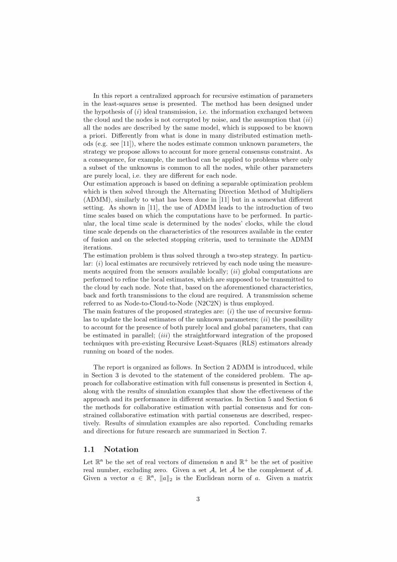
Observe that the parameters ρ1, ρ2 ∈ R+ have to be tuned. To assess howthe choice of these two parameters affects the satisfaction of (87), consider thenumber of steps the local estimates violate the constraints over the estimationhorizon T , {N b
i }3i=1. Assuming that “negligible” violations of the constraintsare allowed, (87) are supposed to be violated if the estimated parameters falloutside the interval Bn = [ `n−10−4 un+10−4 ]. Considering the set of constraints
S2 = {`n = [ 0.19 θn,2−0.1 0.79 ] , upn = [ 0.21 θn,2+0.1 0.81 ]},
Figure 14 shows the average percentage of violations over the N agents obtainedfixing ρ2 = 0.1 and choosing
ρ1 = {10−5, 10−4, 10−3, 10−2.10−1, 1, 10, 20}.
Observe that if ρ1 dominates over ρ2 the number of violations tends to decrease,as in the augmented Lagrangian (87) are weighted more than the consensusconstraint. However, if ρ1/ρ2 > 100, {N b
i }3i=1 tend to slightly increase. Itis thus important to trade-off between the weights attributed to (87) and theconsensus constraint. To evaluate how the stiffness of the constraints affects thechoice of the parameters, {N b
i }3i=1 are computed considering three different setsof box constraints
S1 = {`n = [ 0.195 θn,2−0.05 0.795 ] , upn = [ 0.205 θn,2+0.05 0.805 ]},S2 = {`n = [ 0.19 θn,2−0.1 0.79 ] , upn = [ 0.21 θn,2+0.1 0.81 ]},S3 = {`n = [ 0.15 θn,2−0.5 0.75 ] , upn = [ 0.25 θn,2+0.5 0.85 ]}.
The resulting {N bi }3i=1 are reported in Figure 15. Note that also in this case the
higher the ratio ρ1/ρ2 is, the smaller {N bi }3i=1 are. However, also in this case,
the constraint violations tend to increase for ρ1/ρ2 > 100.
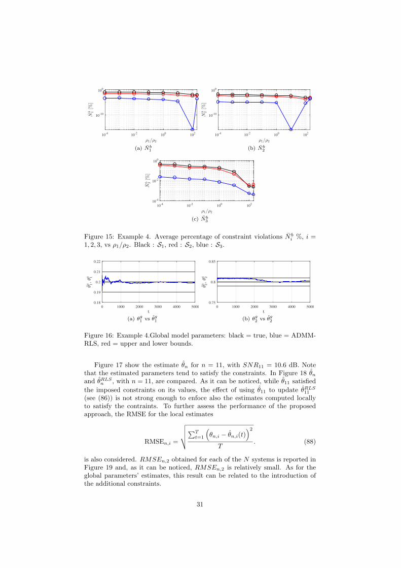
Focusing on the assessment of ADMM-RLS performances when the set ofconstraints is S2, Figure 16 shows the global estimates obtained using the sameinitial conditions and forgetting factors as in Section 6, with ρ1 = 10 and ρ2 =0.1. Note that the global estimates satisfy (87), showing that the constraints onthe global estimate are automatically enforced imposing θn ∈ Cn. As it concernsthe RMSEs for θg (43), they are equal to:
RMSEg1 = 0.001 and RMSEg2 = 0.006,
and their relatively small values can be related to the introduction of the addi-tional constraints, that allow to limit the resulting estimation error.
30
10-4
10-2
100
102
10-10
100
(a) Nb1
10-4
10-2
100
102
10-10
100
(b) Nb2
10-4
10-2
100
102
10-4
10-2
100
(c) Nb3
Figure 15: Example 4. Average percentage of constraint violations N bi %, i =
1, 2, 3, vs ρ1/ρ2. Black : S1, red : S2, blue : S3.
0 1000 2000 3000 4000 5000
0.18
0.19
0.2
0.21
0.22
(a) θg1 vs θg1
0 1000 2000 3000 4000 5000
0.75
0.8
0.85
(b) θg2 vs θg2
Figure 16: Example 4.Global model parameters: black = true, blue = ADMM-RLS, red = upper and lower bounds.
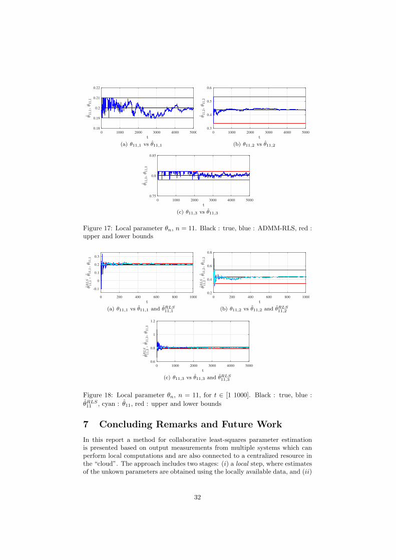
Figure 17 show the estimate θn for n = 11, with SNR11 = 10.6 dB. Notethat the estimated parameters tend to satisfy the constraints. In Figure 18 θnand θRLSn , with n = 11, are compared. As it can be noticed, while θ11 satisfied
the imposed constraints on its values, the effect of using θ11 to update θRLS11
(see (86)) is not strong enough to enfoce also the estimates computed locallyto satisfy the contraints. To further assess the performance of the proposedapproach, the RMSE for the local estimates
RMSEn,i =
√√√√∑Tt=1
(θn,i − θn,i(t)
)2T
. (88)
is also considered. RMSEn,2 obtained for each of the N systems is reported inFigure 19 and, as it can be noticed, RMSEn,2 is relatively small. As for theglobal parameters’ estimates, this result can be related to the introduction ofthe additional constraints.
31
0 1000 2000 3000 4000 5000
0.18
0.19
0.2
0.21
0.22
(a) θ11,1 vs θ11,1
0 1000 2000 3000 4000 5000
0.3
0.4
0.5
0.6
(b) θ11,2 vs θ11,2
0 1000 2000 3000 4000 5000
0.75
0.8
0.85
(c) θ11,3 vs θ11,3
Figure 17: Local parameter θn, n = 11. Black : true, blue : ADMM-RLS, red :upper and lower bounds
0 200 400 600 800 1000
-0.1
0
0.1
0.2
0.3
(a) θ11,1 vs θ11,1 and θRLS11,1
0 200 400 600 800 1000
0.2
0.4
0.6
0.8
(b) θ11,2 vs θ11,2 and θRLS11,2
0 1000 2000 3000 4000 5000
0.6
0.8
1
1.2
(c) θ11,3 vs θ11,3 and θRLS11,3
Figure 18: Local parameter θn, n = 11, for t ∈ [1 1000]. Black : true, blue :
θRLS11 , cyan : θ11, red : upper and lower bounds
7 Concluding Remarks and Future Work
In this report a method for collaborative least-squares parameter estimationis presented based on output measurements from multiple systems which canperform local computations and are also connected to a centralized resource inthe “cloud”. The approach includes two stages: (i) a local step, where estimatesof the unkown parameters are obtained using the locally available data, and (ii)
32

10 20 30 40 50 60 70 80 90 100
0
0.01
0.02
0.03
0.04
Figure 19: RMSE2 for each agent n, n = 1, . . . , N .
a global stage, performed on the cloud, where the local estimates are fused.Future research will address extentions of the method to the nonlinear andmulti-class consensus cases. Moreover, an alternative solution of the problemwill be studied so to replace the transmission policy required now, i.e. N2C2N,with a Node-to-Cloud (N2C) communication scheme. This change should allowto alleviate problems associated with the communication latency between thecloud and the nodes. Moreover, it should enable to obtain local estimators thatrun independently from the data transmitted by the cloud, and not requiringsynchronous processing by the nodes and “cloud”. Other, solutions to furtherreduce the trasmission complexity and to obtain an asynchronous scheme withthe same characteristics as the one presented in this report will be investigated.
A Centralized RLS
Consider problem (12), with the cost functions given by
fn(θn) =1
2
T∑t=1
‖yn(t)− (Xn(t))′θn‖22.
The addressed problem can be solved in a fully centralized fashion, if at each stept all the agents transmit the collected data pairs {yn(t), Xn(t)}, n = 1, . . . , N ,to the “cloud”. This allows the creation of the lumped measurement vector andregressor, given by
y(t) =[y1(t)′ . . . yN (t)′
]′ ∈ RN ·ny×1,
X(t) =[X1(t)′ . . . XN (t)′
]′ ∈ Rnθ×ny·N .(89)
Through the introduction of the lumped vectors, (12) with fn as in (20) isequivalent to
minθg
1
2
T∑t=1
∥∥y(t)− (X(t))′θg∥∥22. (90)
The estimate for the unknown parameters θg can thus be retrieved applyingstandard RLS (see [9]), i.e. performing at each step t the following iterations
K(t) = φ(t− 1)X(t)(ID + (X(t))′φ(t− 1)X(t)
)−1, (91)
φ(t) =(Inθ −K(t)(X(t))′
)φ(t− 1), (92)
θg(t) = θg(t− 1) +K(t)(y(t)− (X(t))′θg(t− 1)
), (93)
with D = N · ny × 1.
33

References
[1] F. Boem, Y. Xu, C. Fischione, and T. Parisini. A distributed estimationmethod for sensor networks based on pareto optimization. In 2012 IEEE51st IEEE Conference on Decision and Control (CDC), pages 775–781, Dec2012.
[2] S. Boyd, N. Parikh, E. Chu, B. Peleato, and J. Eckstein. Distributedoptimization and statistical learning via the alternating direction methodof multipliers. Found. Trends Mach. Learn., 3(1):1–122, January 2011.
[3] F. S. Cattivelli, C. G. Lopes, and A. H. Sayed. Diffusion recursive least-squares for distributed estimation over adaptive networks. IEEE Transac-tions on Signal Processing, 56(5):1865–1877, May 2008.
[4] Pedro A. Forero, Alfonso Cano, and Georgios B. Giannakis. Consensus-based distributed support vector machines. The Journal of Machine Learn-ing Research, 11:1663–1707, Aug 2010.
[5] F. Garin and L. Schenato. A Survey on Distributed Estimation and ControlApplications Using Linear Consensus Algorithms, pages 75–107. SpringerLondon, London, 2010.
[6] M.N. Howell, J.P. Whaite, P. Amatyakul, Y.K. Chin, M.A. Salman, C.H.Yen, and M.T. Riefe. Brake pad prognosis system, Apr 2010. US Patent7,694,555.
[7] Z. Li, I. Kolmanovsky, E. Atkins, J. Lu, D. P. Filev, and J. Michelini.Road risk modeling and cloud-aided safety-based route planning. IEEETransactions on Cybernetics, 46(11):2473–2483, Nov 2016.
[8] Z. Li, I. Kolmanovsky, E. M. Atkins, J. Lu, D. P. Filev, and Y. Bai.Road disturbance estimation and cloud-aided comfort-based route plan-ning. IEEE Transactions on Cybernetics, PP(99):1–13, 2017.
[9] L. Ljung. System identification: theory for the user. Prentice-Hall Engle-wood Cliffs, NJ, 1999.
[10] C. G. Lopes and A. H. Sayed. Incremental adaptive strategies over dis-tributed networks. IEEE Transactions on Signal Processing, 55(8):4064–4077, Aug 2007.
[11] G. Mateos, I. D. Schizas, and G. B. Giannakis. Distributed recursive least-squares for consensus-based in-network adaptive estimation. IEEE Trans-actions on Signal Processing, 57(11):4583–4588, Nov 2009.
[12] Peter M. Mell and Timothy Grance. Sp 800-145. the nist definition of cloudcomputing. Technical report, Gaithersburg, MD, United States, 2011.
[13] R. Olfati-Saber. Distributed kalman filtering for sensor networks. In 200746th IEEE Conference on Decision and Control, pages 5492–5498, Dec2007.
34

[14] E. Ozatay, S. Onori, J. Wollaeger, U. Ozguner, G. Rizzoni, D. Filev,J. Michelini, and S. Di Cairano. Cloud-based velocity profile optimiza-tion for everyday driving: A dynamic-programming-based solution. IEEETransactions on Intelligent Transportation Systems, 15(6):2491–2505, Dec2014.
[15] E. Taheri, O. Gusikhin, and I. Kolmanovsky. Failure prognostics for in-tank fuel pumps of the returnless fuel systems. In Dynamic Systems andControl Conference, Oct 2016.
35