Technical Report TR-2014-14

Comparison of a steady-state Magic Formula tire modelwith a commercial software implementation

Justin Madsen and Alex Dirr

October 3, 2014

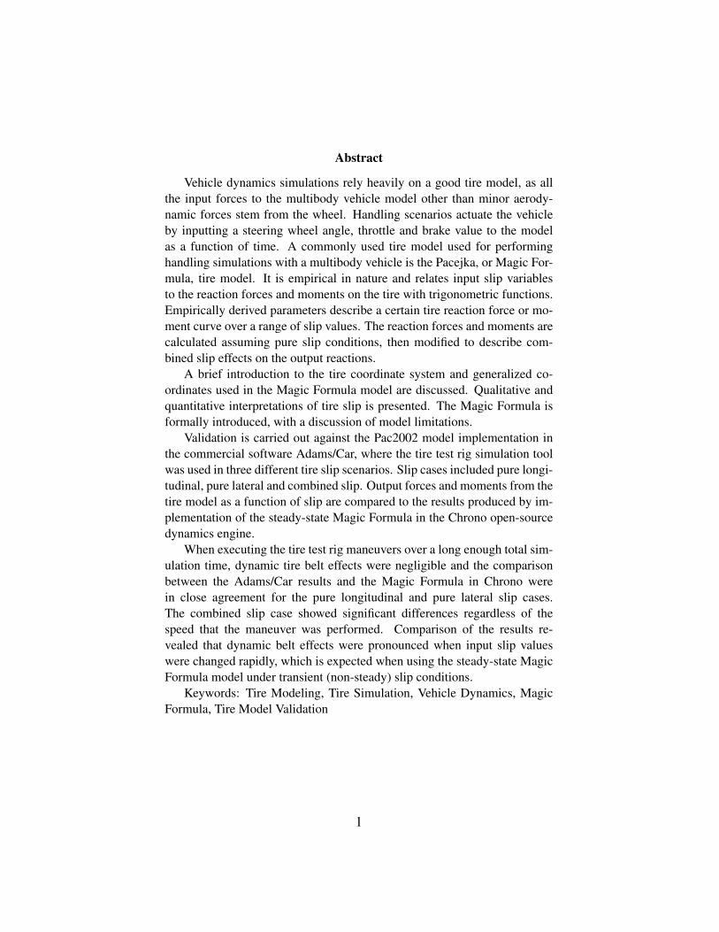
Abstract

Vehicle dynamics simulations rely heavily on a good tire model, as allthe input forces to the multibody vehicle model other than minor aerody-namic forces stem from the wheel. Handling scenarios actuate the vehicleby inputting a steering wheel angle, throttle and brake value to the modelas a function of time. A commonly used tire model used for performinghandling simulations with a multibody vehicle is the Pacejka, or Magic For-mula, tire model. It is empirical in nature and relates input slip variablesto the reaction forces and moments on the tire with trigonometric functions.Empirically derived parameters describe a certain tire reaction force or mo-ment curve over a range of slip values. The reaction forces and moments arecalculated assuming pure slip conditions, then modified to describe com-bined slip effects on the output reactions.

A brief introduction to the tire coordinate system and generalized co-ordinates used in the Magic Formula model are discussed. Qualitative andquantitative interpretations of tire slip is presented. The Magic Formula isformally introduced, with a discussion of model limitations.

Validation is carried out against the Pac2002 model implementation inthe commercial software Adams/Car, where the tire test rig simulation toolwas used in three different tire slip scenarios. Slip cases included pure longi-tudinal, pure lateral and combined slip. Output forces and moments from thetire model as a function of slip are compared to the results produced by im-plementation of the steady-state Magic Formula in the Chrono open-sourcedynamics engine.

When executing the tire test rig maneuvers over a long enough total sim-ulation time, dynamic tire belt effects were negligible and the comparisonbetween the Adams/Car results and the Magic Formula in Chrono werein close agreement for the pure longitudinal and pure lateral slip cases.The combined slip case showed significant differences regardless of thespeed that the maneuver was performed. Comparison of the results re-vealed that dynamic belt effects were pronounced when input slip valueswere changed rapidly, which is expected when using the steady-state MagicFormula model under transient (non-steady) slip conditions.

Keywords: Tire Modeling, Tire Simulation, Vehicle Dynamics, MagicFormula, Tire Model Validation

1

Contents1 Introduction 3

2 Tire coordinate system and important variables 3

3 Tire slip 53.1 Qualitative explanation of tire slip . . . . . . . . . . . . . . . . . 53.2 Slip definitions . . . . . . . . . . . . . . . . . . . . . . . . . . . 6

4 Magic Formula 6

5 Model validation 85.1 Pure longitudinal slip case . . . . . . . . . . . . . . . . . . . . . 95.2 Pure lateral slip case . . . . . . . . . . . . . . . . . . . . . . . . 95.3 Combined slip case . . . . . . . . . . . . . . . . . . . . . . . . . 12

6 Conclusion 15

2

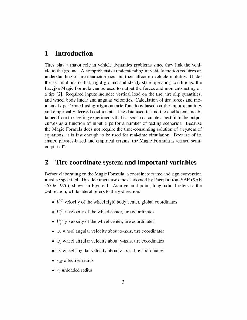
1 IntroductionTires play a major role in vehicle dynamics problems since they link the vehi-cle to the ground. A comprehensive understanding of vehicle motion requires anunderstanding of tire characteristics and their effect on vehicle mobility. Underthe assumptions of flat, rigid ground and steady-state operating conditions, thePacejka Magic Formula can be used to output the forces and moments acting ona tire [2]. Required inputs include: vertical load on the tire, tire slip quantities,and wheel body linear and angular velocities. Calculation of tire forces and mo-ments is performed using trigonometric functions based on the input quantitiesand empirically derived coefficients. The data used to find the coefficients is ob-tained from tire-testing experiments that is used to calculate a best fit to the outputcurves as a function of input slips for a number of testing scenarios. Becausethe Magic Formula does not require the time-consuming solution of a system ofequations, it is fast enough to be used for real-time simulation. Because of itsshared physics-based and empirical origins, the Magic Formula is termed semi-empirical”.

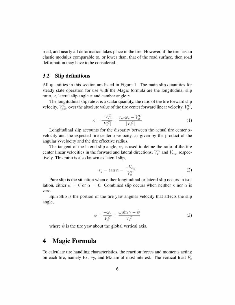
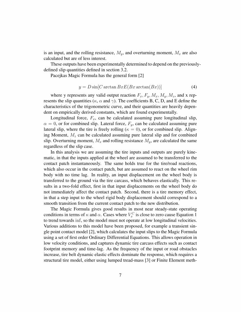
2 Tire coordinate system and important variablesBefore elaborating on the Magic Formula, a coordinate frame and sign conventionmust be specified. This document uses those adopted by Pacejka from SAE (SAEJ670e 1976), shown in Figure 1. As a general point, longitudinal refers to thex-direction, while lateral refers to the y-direction.

• ~V C velocity of the wheel rigid body center, global coordinates

• V Cx x-velocity of the wheel center, tire coordinates

• V Cy y-velocity of the wheel center, tire coordinates

• ωx wheel angular velocity about x-axis, tire coordinates

• ωy wheel angular velocity about y-axis, tire coordinates

• ωz wheel angular velocity about z-axis, tire coordinates

• reff effective radius

• r0 unloaded radius

3

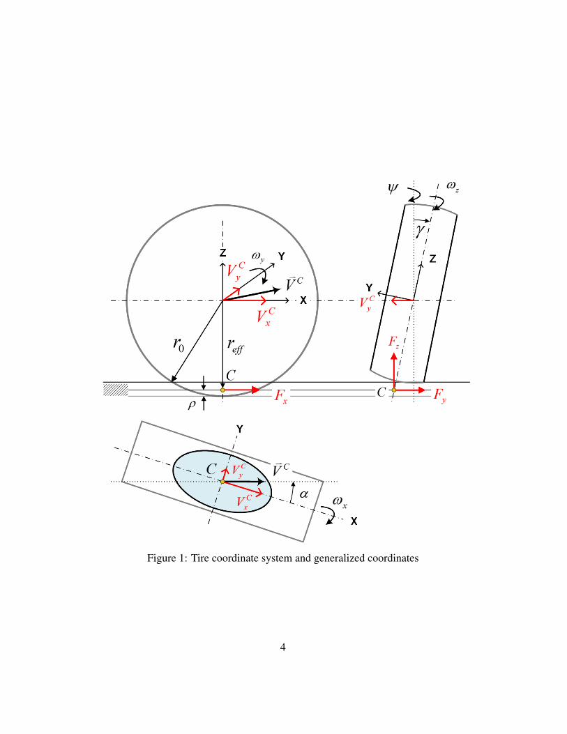
Figure 1: Tire coordinate system and generalized coordinates

4

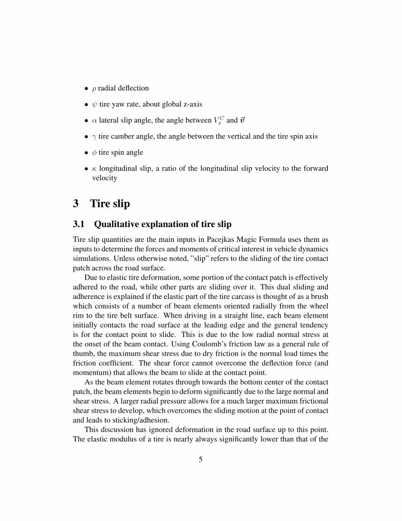
• ρ radial deflection

• ψ tire yaw rate, about global z-axis

• α lateral slip angle, the angle between V Cx and ~v

• γ tire camber angle, the angle between the vertical and the tire spin axis

• φ tire spin angle

• κ longitudinal slip, a ratio of the longitudinal slip velocity to the forwardvelocity

3 Tire slip

3.1 Qualitative explanation of tire slipTire slip quantities are the main inputs in Pacejkas Magic Formula uses them asinputs to determine the forces and moments of critical interest in vehicle dynamicssimulations. Unless otherwise noted, ”slip” refers to the sliding of the tire contactpatch across the road surface.

Due to elastic tire deformation, some portion of the contact patch is effectivelyadhered to the road, while other parts are sliding over it. This dual sliding andadherence is explained if the elastic part of the tire carcass is thought of as a brushwhich consists of a number of beam elements oriented radially from the wheelrim to the tire belt surface. When driving in a straight line, each beam elementinitially contacts the road surface at the leading edge and the general tendencyis for the contact point to slide. This is due to the low radial normal stress atthe onset of the beam contact. Using Coulomb’s friction law as a general rule ofthumb, the maximum shear stress due to dry friction is the normal load times thefriction coefficient. The shear force cannot overcome the deflection force (andmomentum) that allows the beam to slide at the contact point.

As the beam element rotates through towards the bottom center of the contactpatch, the beam elements begin to deform significantly due to the large normal andshear stress. A larger radial pressure allows for a much larger maximum frictionalshear stress to develop, which overcomes the sliding motion at the point of contactand leads to sticking/adhesion.

This discussion has ignored deformation in the road surface up to this point.The elastic modulus of a tire is nearly always significantly lower than that of the

5

road, and nearly all deformation takes place in the tire. However, if the tire has anelastic modulus comparable to, or lower than, that of the road surface, then roaddeformation may have to be considered.

3.2 Slip definitionsAll quantities in this section are listed in Figure 1. The main slip quantities forsteady state operation for use with the Magic formula are the longitudinal slipratio, κ, lateral slip angle α and camber angle γ.

The longitudinal slip rate κ is a scalar quantity, the ratio of the tire forward slipvelocity, V C

s,x, over the absolute value of the tire center forward linear velocity, V Cx ,

κ =−V C

s,x

|V Cx |

=reffωy − V C

x

|V Cx |

(1)

Longitudinal slip accounts for the disparity between the actual tire center x-velocity and the expected tire center x-velocity, as given by the product of theangular y-velocity and the tire effective radius.

The tangent of the lateral slip angle, α, is used to define the ratio of the tirecenter linear velocities in the forward and lateral directions, V C

x and Vc,y, respec-tively. This ratio is also known as lateral slip,

sy = tanα =−Vc,yV Cx

(2)

Pure slip is the situation when either longitudinal or lateral slip occurs in iso-lation, either κ = 0 or α = 0. Combined slip occurs when neither κ nor α iszero.

Spin Slip is the portion of the tire yaw angular velocity that affects the slipangle,

φ =−ωzV Cx

=ω sin γ − ψ̇

V Cx

(3)

where ψ̇ is the tire yaw about the global vertical axis.

4 Magic FormulaTo calculate tire handling characteristics, the reaction forces and moments actingon each tire, namely Fx, Fy, and Mz are of most interest. The vertical load Fz

6

is an input, and the rolling resistance, My, and overturning moment, Mx are alsocalculated but are of less interest.

These outputs have been experimentally determined to depend on the previously-defined slip quantities defined in section 3.2.

Pacejkas Magic Formula has the general form [2]

y = D sin[C arctanBxE(Bx arctan(Bx))] (4)

where y represents any valid output reaction Fx, Fy,Mx,My,Mz, and x rep-resents the slip quantities (κ, α and γ). The coefficients B, C, D, and E define thecharacteristics of the trigonometric curve, and their quantities are heavily depen-dent on empirically derived constants, which are found experimentally.

Longitudinal force, Fx, can be calculated assuming pure longitudinal slip,α = 0, or for combined slip. Lateral force, Fy, can be calculated assuming purelateral slip, where the tire is freely rolling (κ = 0), or for combined slip. Align-ing Moment, Mz can be calculated assuming pure lateral slip and for combinedslip. Overturning moment, Mx and rolling resistance My, are calculated the sameregardless of the slip case.

In this analysis we are assuming the tire inputs and outputs are purely kine-matic, in that the inputs applied at the wheel are assumed to be transferred to thecontact patch instantaneously. The same holds true for the tire/road reactions,which also occur in the contact patch, but are assumed to react on the wheel rimbody with no time lag. In reality, an input displacement on the wheel body istransferred to the ground via the tire carcass, which behaves elastically. This re-sults in a two-fold effect, first in that input displacements on the wheel body donot immediately affect the contact patch. Second, there is a tire memory effect,in that a step input to the wheel rigid body displacement should correspond to asmooth transition from the current contact patch to the new distribution.

The Magic Formula gives good results in most near steady-state operatingconditions in terms of κ and α. Cases where V C

x is close to zero cause Equation 1to trend towards inf, so the model must not operate at low longitudinal velocities.Various additions to this model have been proposed, for example a transient sin-gle point contact model [2], which calculates the input slips to the Magic Formulausing a set of first order Ordinary Differential Equations. This allows operation inlow velocity conditions, and captures dynamic tire carcass effects such as contactfootprint memory and time-lag. As the frequency of the input or road obstaclesincrease, tire belt dynamic elastic effects dominate the response, which requires astructural tire model, either using lumped tread-mass [3] or Finite Element meth-

7

ods [4, 5, 6, 7].

5 Model validationAdams/Car is a widely used and validated commercial multibody dynamics sim-ulation software tool, and has an implementation of the Pac2002 model that in-cludes the Magic Formula steady-state equations as well as transient single pointcontact models. It will be used to compare and validate the performance of theMagic Formula implementation in Chrono. The tire model in Adams/Car will bereferred to as ”transient”, while the Chrono model is termed the ”steady-state”tire.

The single point contact models are either linear or non-linear, depending on ifthe mass of the contact patch is included in the dynamics. These models provideimproved calculation of slip values during non-steady conditions based on thesolution of a set of linear ODEs. For example, a step input to the steering wheelresults in a step input in the lateral slip angle; however, the slip values in thecontact patch do not change instantaneously, but smoothly to a new steady-statevalue (if the steering wheel input is not changed further). The tire can handleevent with frequencies of up to 8 and 15 Hz, for the linear and non-linear models,respectively. Both time-lag and tire memory effects in the calculated reactions area direct result of using single contact point models to consider the compliance ofthe tire carcass during non-steady state maneuvers. These must be kept in mindwhen setting up the Adams/Car tire test rig simulations.

Three separate slip scenarios are used for comparison. The simulation param-eters of the Adams/Car tire test rig are described, with an emphasis on simulationsettings that may induce non-steady state (e.g., transient) effects in the Adams/Cartire model. A similar test is run using the steady-state Magic formula implementedin Chrono. Outputs are recorded and compared for forces and moments as a func-tion of slip.

Common for both simulations are:

• A tire parameter file corresponding to a 235 60R 16 type tire is used.

• Tire vertical load is 8000 N

• Pure longitudinal slip cases inputs range from [κmin, κmax] vs. time

8

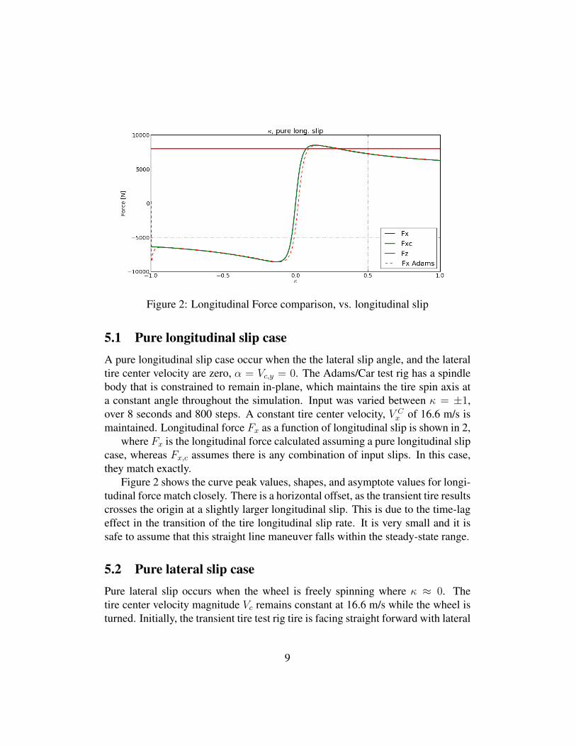
Figure 2: Longitudinal Force comparison, vs. longitudinal slip

5.1 Pure longitudinal slip caseA pure longitudinal slip case occur when the the lateral slip angle, and the lateraltire center velocity are zero, α = Vc,y = 0. The Adams/Car test rig has a spindlebody that is constrained to remain in-plane, which maintains the tire spin axis ata constant angle throughout the simulation. Input was varied between κ = ±1,over 8 seconds and 800 steps. A constant tire center velocity, V C

x of 16.6 m/s ismaintained. Longitudinal force Fx as a function of longitudinal slip is shown in 2,

where Fx is the longitudinal force calculated assuming a pure longitudinal slipcase, whereas Fx,c assumes there is any combination of input slips. In this case,they match exactly.

Figure 2 shows the curve peak values, shapes, and asymptote values for longi-tudinal force match closely. There is a horizontal offset, as the transient tire resultscrosses the origin at a slightly larger longitudinal slip. This is due to the time-lageffect in the transition of the tire longitudinal slip rate. It is very small and it issafe to assume that this straight line maneuver falls within the steady-state range.

5.2 Pure lateral slip casePure lateral slip occurs when the wheel is freely spinning where κ ≈ 0. Thetire center velocity magnitude Vc remains constant at 16.6 m/s while the wheel isturned. Initially, the transient tire test rig tire is facing straight forward with lateral

9

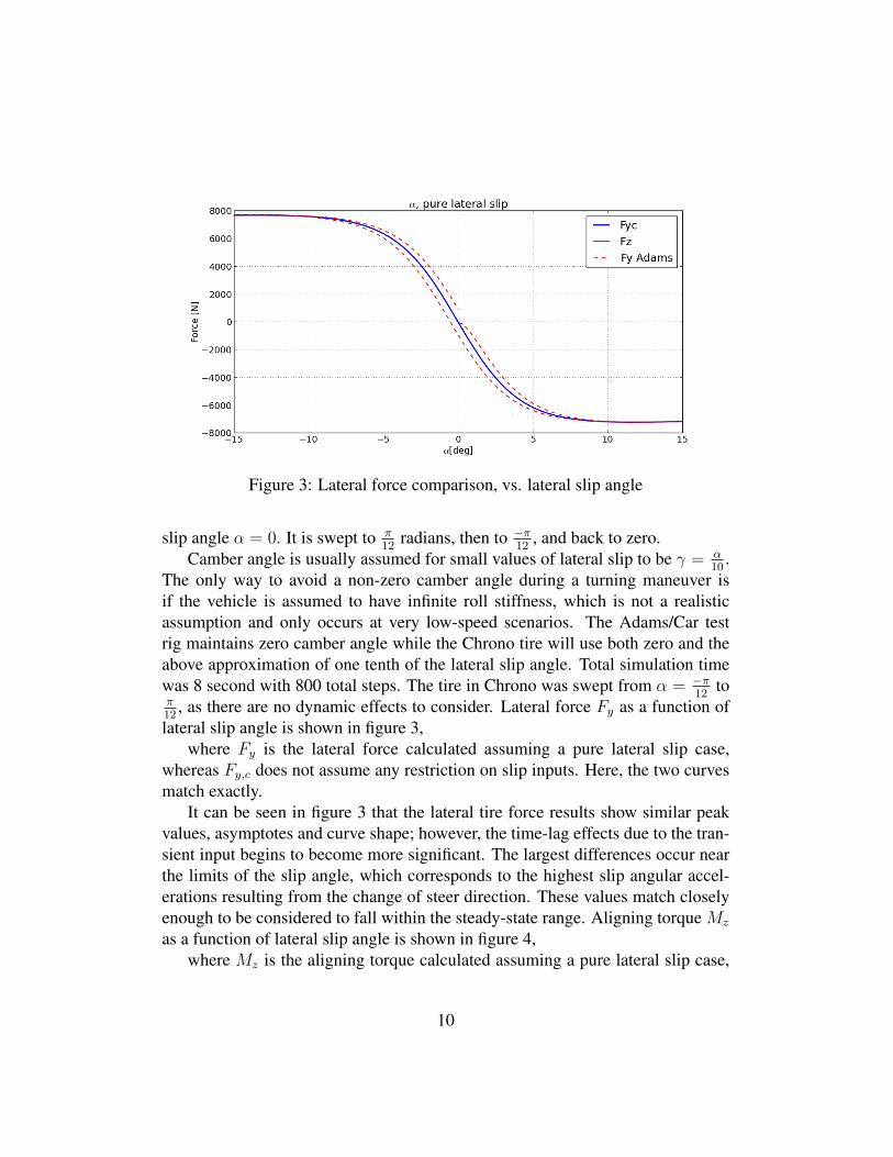
Figure 3: Lateral force comparison, vs. lateral slip angle

slip angle α = 0. It is swept to π12

radians, then to −π12

, and back to zero.Camber angle is usually assumed for small values of lateral slip to be γ = α

10.

The only way to avoid a non-zero camber angle during a turning maneuver isif the vehicle is assumed to have infinite roll stiffness, which is not a realisticassumption and only occurs at very low-speed scenarios. The Adams/Car testrig maintains zero camber angle while the Chrono tire will use both zero and theabove approximation of one tenth of the lateral slip angle. Total simulation timewas 8 second with 800 total steps. The tire in Chrono was swept from α = −π

12to

π12

, as there are no dynamic effects to consider. Lateral force Fy as a function oflateral slip angle is shown in figure 3,

where Fy is the lateral force calculated assuming a pure lateral slip case,whereas Fy,c does not assume any restriction on slip inputs. Here, the two curvesmatch exactly.

It can be seen in figure 3 that the lateral tire force results show similar peakvalues, asymptotes and curve shape; however, the time-lag effects due to the tran-sient input begins to become more significant. The largest differences occur nearthe limits of the slip angle, which corresponds to the highest slip angular accel-erations resulting from the change of steer direction. These values match closelyenough to be considered to fall within the steady-state range. Aligning torque Mz

as a function of lateral slip angle is shown in figure 4,where Mz is the aligning torque calculated assuming a pure lateral slip case,

10

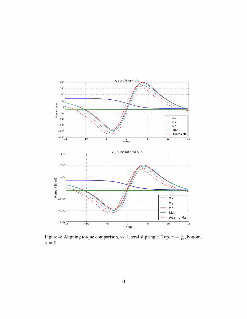
Figure 4: Aligning torque comparison, vs. lateral slip angle. Top, γ = α10

, bottom,γ = 0

11

where Mz,c is for any combination of slip inputs. The curves in figure 4 for align-ing torque match very closely, but not exactly, likely due to dynamic tread effects.The top plot in figure 4 where γ = α

10, shows small difference when compared to

the bottom where γ = 0.Similar conclusions to the lateral force can be drawn for the aligning torque

for the pure lateral slip case. Small dynamic effects cause the transient tire align-ing moment to develop more slowly from the initial conditions, which preventsit from reaching the peak value seen by the Chrono steady-state results. In thenegative aligning moment region, the opposite effect occurs, where the transienttire overshoots the peak value seen by the steady-state model. This is likely dueto the momentum of sweeping the tire from maximum positive to negative valuesof α, which is reflected in the transient tire model aligning torque results. Thesevalues match closely enough to fall within the steady-state range; however, it issuggested that lateral slip angle α be adjusted more gradually if accurate aligningtorque calculations are needed.

5.3 Combined slip caseLateral slip angle α is swept in the range of± π

12radians, where the Adams/Car test

rig applies this input in the same sequence as was described in 5.2. Longitudinalslip rate was varied simultaneously in the range κ = ±1, over 8 seconds and800 steps. Camber angle is usually assumed for small values of lateral slip to beγ = α

10. The tire center velocity magnitude Vc remains constant at 16.6 m/s while

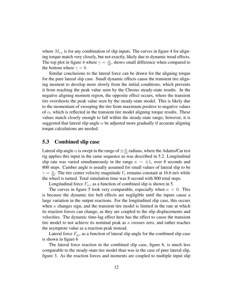
the wheel is turned. Total simulation time was 8 second with 800 total steps.Longitudinal force Fx,c as a function of combined slip is shown in 5.The curves in figure 5 look very comparable, especially when κ < 0. This

is because the dynamic tire belt effects are negligible until the inputs cause alarge variation in the output reactions. For the longitudinal slip case, this occurswhen κ changes sign, and the transient tire model is limited in the rate at whichits reaction forces can change, as they are coupled to the slip displacements andvelocities. The dynamic time-lag effect here has the effect to cause the transienttire model to not achieve its nominal peak as κ crosses zero, and rather reachesthe asymptote value as a reaction peak instead.

Lateral force Fy,c as a function of lateral slip angle for the combined slip caseis shown in figure 6

The lateral force reaction in the combined slip case, figure 6, is much lesscomparable to the steady-state tire model than was in the case of pure lateral slip,figure 3. As the reaction forces and moments are coupled to multiple input slip

12

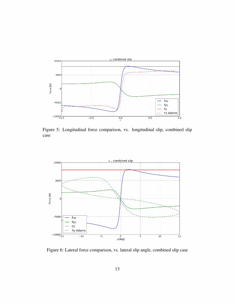
Figure 5: Longitudinal force comparison, vs. longitudinal slip, combined slipcase

Figure 6: Lateral force comparison, vs. lateral slip angle, combined slip case

13

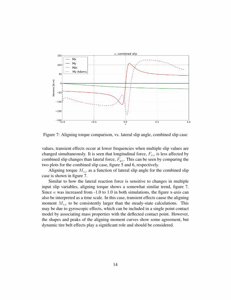
Figure 7: Aligning torque comparison, vs. lateral slip angle, combined slip case

values, transient effects occur at lower frequencies when multiple slip values arechanged simultaneously. It is seen that longitudinal force, Fx,c is less affected bycombined slip changes than lateral force, Fy,c. This can be seen by comparing thetwo plots for the combined slip case, figure 5 and 6, respectively.

Aligning torque Mz,c as a function of lateral slip angle for the combined slipcase is shown in figure 7.

Similar to how the lateral reaction force is sensitive to changes in multipleinput slip variables, aligning torque shows a somewhat similar trend, figure 7.Since κ was increased from -1.0 to 1.0 in both simulations, the figure x-axis canalso be interpreted as a time scale. In this case, transient effects cause the aligningmoment Mz,c to be consistently larger than the steady-state calculations. Thismay be due to gyroscopic effects, which can be included in a single point contactmodel by associating mass properties with the deflected contact point. However,the shapes and peaks of the aligning moment curves show some agreement, butdynamic tire belt effects play a significant role and should be considered.

14

6 ConclusionA basic steady-state Magic Formula tire model was implemented in the Chronomultibody dynamics software framework. It was tested and compared to an im-plementation in the COTS Adams/Car, showing good agreement when changes tothe input variables were modest with respect to time. Differences in the outputforces and torques are seen when the input variables are changed quickly. Here,the transient single point contact tire model present in the commercial softwareproduced slightly different outputs.

Comparing similar simulations under less transient conditions was achievedby running simulations with longer total time durations, allowing the rate of changeof the input variables to remain small. By remaining close to steady-state condi-tions, the output reaction forces and moments trend towards the steady-state so-lution in Chrono. However, when slip quantities are changed simultaneously, thelateral force and aligning moment show considerable differences between the twomodels. The steady-state tire model should be used with care when both α and κchange at the same time. For example, any handling event where acceleration/de-celeration and turning are performed simultaneously.

In order to consider the dynamic tire belt effects on the reaction forces andmoments, at the very minimum the the compliance of the tire must be considered.A linear and non-linear single point transient tire model is presented by Pacejka[2], which increases the frequency the tire model can accurately model to approxi-mately 8 and 15 Hz, respectively. It also avoids the errors associated with low for-ward tire velocity values, as these types of models can be used as a pre-processorto the input slip quantities for the steady-state Magic Formula equations.

Accurately simulating vehicle dynamics in a virtual environment requires theability to handle a large range of driver inputs to the vehicle, while also accom-modating regularly encountered maneuvers and scenarios (e.g., braking to a stop,parallel parking, etc.) A follow-up report will perform similar comparisons withCOTS implementations of the Pac2002 tire model with the single point contactmodel implemented in Chrono.

References[1] H. Mazhar, T. Heyn, A. Pazouki, D. Melanz, A. Seidl, A. Bartholomew,

A. Tasora, and D. Negrut. Chrono: a parallel multi-physics library for rigid-body, flexible-body, and fluid dynamics. Mech. Sci., 4(1):49–64, 2013.

15

[2] H. Pacejka. Tire and vehicle dynamics. Elsevier, 2005.

[3] M. Gipser. Ftire - the tire simulation model for all applications related tovehicle dynamics. Vehicle System Dynamics, 45(139-151):139–151, 2007.

[4] H. Sugiyama and Y. Suda. Non-linear elastic ring tyre model using the ab-solute nodal coordinate formulation. Proc. IMechE Part K: J. Multi-bodyDynamics, 223:211–219, 2009.

[5] C. W. Fervers. Improved FEM simulation model for tiresoil interaction. Jour-nal of Terramechanics, 41(2):87–100, 2004.

[6] S. Shoop. Finite Element Modeling of Tire-Terrain Interaction. Thesis, Uni-versity of Michigan, 2001.

[7] K. Xia and Y. Yang. Three-dimensional finite element modeling of tire/groundinteraction. International journal for numerical and analytical methods ingeomechanics, 36(4):498–516, 2012.

16