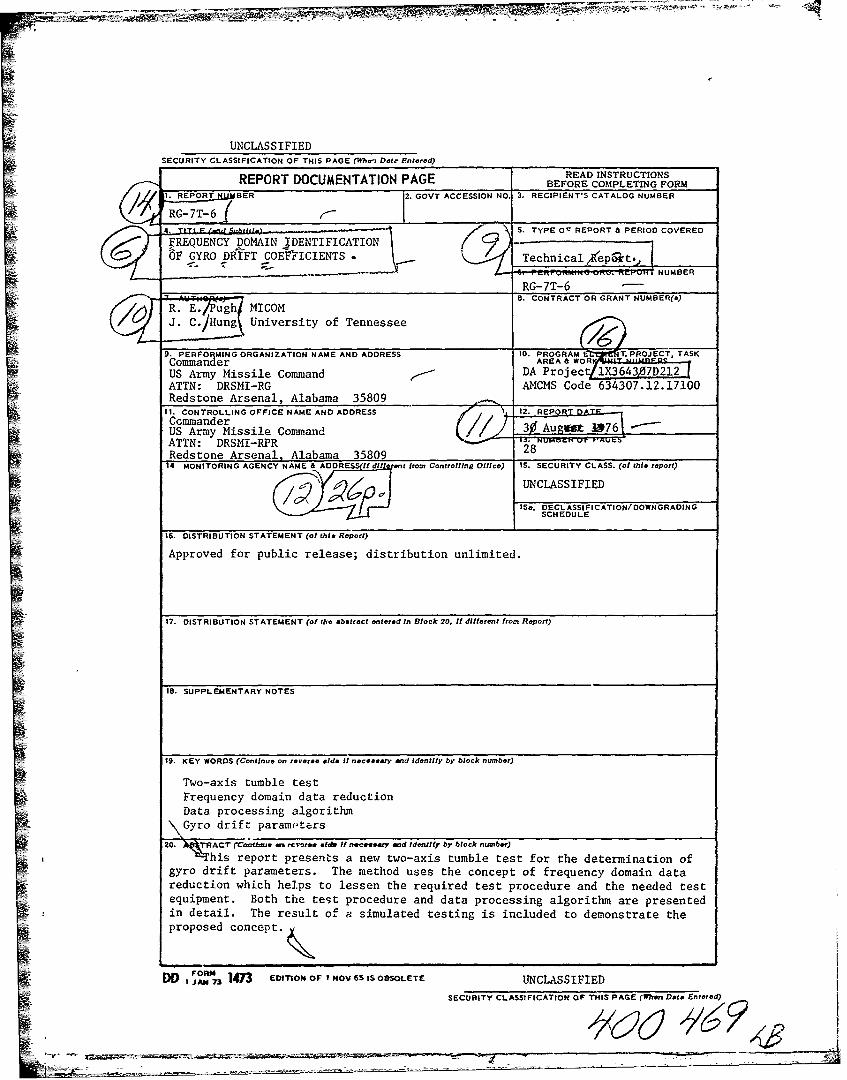
TECHNICAL REPORT RG-7TG

FREQUENCY DOMAIN IDENTIFICATIONOF GYRO DRIFT COEFFICIENTS

R. E. PughGuidance and Control DirectorateUS Army Missile Rosearch, Development and Esgineering LaboratoryUS Army Missile CommandRedstone Arsenal, Alabama 35809

and

J. C. HungThe University of TennesseeKnoxville, Tennessee

30 August 1976

Approved for public release; distribution unlimited.

IedetCrie Aront, Alabama 35I09

DISPOSITION INSTRUCTIONS

DESTROY THIS REPORT WHEN IT IS NO LONGER NEEDED. DO NOTRETURN IT TO THE ORIGINATOR.

DISCLAIMER

THE FINDINGS IN THIS REPORT ARE NOT TO BE CONSTRUED AS ANOFFICIAL DEPARTMENT OF THE ARMY POSITION UNLESS SO DESIG-NATED BY OTHER AUTHORIZED DOCUMENTS.

TRADE NAMES

USE OF TRADE NAMES OR MANUFACTURERS IN THIS REPORT DOESNOT CONSTITUTE AN OFFICIAL INDORSEMENT OR APPROVAL OFETHE USE OF SUCH COMMERCIAL HARDWARE OR SOFTWARE.

V t ~ ---.-

UNCLASSIFIEDSECURITY CLASSIFICATION OF THIS PAGE (

1The1 Detr Entered) __________________

REPOT DCUMNTATON AGEREAD INSTRUCTIONSREPOT DCUMNTATON AGEBEFORE COMPLETING FORM

1.RPORT NUBER 2. GOVT ACCESSION No. 3. RECIPIENT'S CATALOG NUMBER

4, II F MH ,,h,1,5. TYPE Oc REPORT 6 PERIOD COVEREDFREQUENCY DOMA7IN JDENTIFICATIONOF GYRO DRIFT COEF-FICIENTSTehia eoti

RG-7T-6-8. CONTRACT OR GRANT NUMBER(&)

/~R. E./Pugh/ MICOMJ.C.j Hung\ University of Tennessee

9. PERFOaMlNG ORGANIZATION NAME AND ADDRESS 10. PROGRAM T.PROJET, TASK

US Army Missile Command .- DA Project 1X3643 07D212-ATTN: DRSMI-RG MM oe63371.70Redstone Arsenal, Alabama 35809 ______________

I I. CONTROLLING OFFICE NAME AND ADDRESS 1mRPCcmmanderUS Army Missile Command 3 u =sJ7ATTN: DRSMI-RPR 8A tRedstone Arsenal, Alabama 35809 ______________

14 MONITORING AGENCY NAME a ADORES If dl! ecuri from Controlling Office) 15. SECURITY CLASS. (of this report)

UNCLASS IFIED

IS&. DECL SSI FICATION/ DOWNGRADING

16. DISTRIBUTION STATEMENT (of this Report)

Approved for public release; distribution unlimited.

17. DISTRIBUTION STATEMENT (of the abstract entered In Block 20, If different from Report)

IS. SUPPLEMENTARY NOTES

19. KEY WORDS (Continue on reverse side If necessay ad Identify by block number)

Two-axis tumble testFrequency domain data reductionData processing algorithm

\Gyro drift paramoters20 4~RC Cahu a reers .1ob If nreceaery macd Idenfify by block number)

This report presents a new two-axis tumble test for the determination ofgyro drift parameters. The method uses the concept of frequency domain datareduction which helps to lessen the required test procedure and the needed testequipment. Both the test procedure and data processing algorithm are presentedin detail. The result o' a simulated testing is included to demonstrate theproposed concept.

D ORO~ 1473 EDITIONs OF I NOV 65 IS OBSOLETE UNCLASSIFIED

SECURITY CLASSIFICATION OF THIS PAGE (NWran Data Entered)

CONTENTS

Page

I. INTRODUCTION .. ........................ 3

II. ANALYTIC MODEL FOR GYRO DRIFT. .. ............... 4

III. A NEW TWO-AXIS TUMBLE TEST .................. 6

IV. DATA PROCESSING ALGORITHM . .. ................. 8

V. SIMULATION RESULT .. ....... ............... 18

VI. CONCLUSION. .......................... 18

REFERENCES. ............................. 23

Appendix. ALGORITHM FOR OLD TWO-AXIS TUMBLE TEST .. ......... 25

I. INTRODUCTION

The use of precision inertial sensors for high performanceapplications demands accurate identification of drift coefficients.I Thic identification technique consists of two parts: testing and datareduction. An acceptable identification technique should be low cost.

I There are at least three different objectives for testing. First,development tests are conducted in laboratories for verifying concepts,gaining intuitions, exploring desired modifications, and searching forproper parameter values. Second, acceptance tests are used by manufac-turers and customers to determine if the specifications are met.Third, calibration tests are used to determine sensor parameters.

This report concerns test and data reduction techniques forsingle-degree-of-freedom gyros. Techniques for two-degree-of-freedomgyros are similar in concept and therefore will not be discussed ii

this report.

The most important aspects of gyro testing for navigation andguidance purposes are those concerned with drift errors. There areat least four different types of testing methods for the determinationof drift parameters [1, 2, 3, 4, 5, and 6]. They are as follows:

a) Six position rate test.

b) Six position static test.

c) Single-axis tumble test.

d) Two-axis tumble test.

All methods require the use of a test table. Both the six positionrate and static tests are time consuming, because they require repeatedreorientation of the gyro and a long settling time after eachreorientation. The single-axis tumble test does not generate sufficientinfcrmation for the determination of drift parameters of a high preci-sion drift model. Among the four methods, the two-axis tumble testis the latest technique. Compared to the others, it has severaladvantages which will be discussed in a later section. However, theknown two-axis tumble test requires the knowledge of the attitude ofthe gyro case at every data taking instant.

This report presents a new two-axis tumble test and data reductiontechnique. The method uses a new concept for obtaining all driftparameters from the measurement record. The concept does not need

[- the knowledge of the gyro case attitude at each data taking instant:.

Thus, much simpler test equipment can be used. The report will firstreview the development of an analytic model for drift parameters. Thetest procedure for the proposed new two-axis tumble test will bedescribed, followed by the development of the data processing algorithm.A comparison between the old and new methods will be made. The result

<V3 A~-~

ii: ED

wz

of a simulation using the proposed technique will be included and dis-cussed. For the convenience of the reader, a list of references andan appendix are attached.

II. ANALYTIC MODEL FOR GYRO DRIFT

Gyro drifts may be classified into three types: constantdrifts, acceleration sensitive drifts, and drifts which are sensitiveto the products of accelerations [7].

The constant drifts are caused by the spring force of flex leadsand by the electrical reaction torques excited on the gimbal. Allconstant drifts will be lumped together and represented by Do.

0

Most of the acceleration sensitive drifts are caused by massunbalance of the gimbal-rotor assembly. This unbalance of mass resultsin a displacement between the gimbal output axis and the mass centerof the gimbal-rotor assembly. This displacement is denoted by d whichis a vector in the three-dimensional space. Let s, i, and 6 be threeunit vectors pointed along the spin reference axis, input axis, and

output axis of the gyro, respectively. Let a be the accelerationvector of the gyru case and m be the mass of the gimbal-rotor assembly.The inertial torque about the output axis due to the acceleration isgiven by

Tm = -m( x a)'3 = m(dia s - dsai)

where "x" and "-" denote cross-product and dot-product, respectively.The subscripts s and i are used to denote those vector components whichare in the directions of s and I, respectively. Because drift islinearly proportional to torque, the mass unbalance drift may be repre-sented by

D = K a + K. a. (1)m s s i

where K and K. are proportionality constants.sME Another source of acceleration sensitive drift is the thermo-

convection torque for a gyro with floated gimbal. When the mass is notbalanced, the thermo-convection in the fluid generates a torque alongthe output axis. This torque is proportional to the mass m, off-centerdisplacement d , and the acceleration component aot where subscript o

denotes the vector components in the direction of o. The correspondingdrift may be represented by

4

Dt Ka (2)th 0 0

where K is a proportional constant. It is noted that Dth is due to the0 t

combined effect of mass unbalance, thermo-convection of the fluid, andthe acceleration of gyro case along the o direction.

The drifts which are sensitive to the product of accelerations arecaused by the deflection of the gimbal assembly under acceleration. Thephenomena is often referred to as anisoelastic effect. The relationshipbetween the deflection and acceleration can be expressed as

A = mCa

where A is the deflection vector and C is a 3 x 3 compliance matrixgiven by

c c. ci

is 11 10

Los coi c

For each double-subscripted element of C, the first subscript denotesthe direction of deflection and the second the direction of acceleration.The (eflection A causes a mass unbalance. Together, they generate atorque about the output axis given by

-m(A a) 2 tc - a. + c a.acss sii I so 1 s

+ca2 2 s+c.a.-c. -c a

sli iss Cioas

Each of the terms in this equation can produce a nonzero average torquein the presence of vibrations of the same frequency. The gyro driftcaused by torque T may be represented by

DK = K a +K a+ K .a a. + K. a.a + K a a . (3)S SS S 1 1 10 1 0 OS 0 S

Adding Equations (1), (2), (3), and D gives the desired analyticmodel of the total drift for the gyro:

5

D D + K a +K.a. + K a + K a2 +K..a2 + K .a a.0 s s 1 0 0 ss s 11 . s3 s 1

+ K. a.a + K aa (4)10 10 0S505

Equation (4) sho,.s that the total drift D consists of nine terms,characterized by drift parameters D and K's. Because a different typeo0of compensation is required for a different type of drift, identificationof these parameters is essential.

III. A NEW TWO-AXIS TUMBLE TEST

Identification of the nine drift paramete:s by testing requiresthat all nine drift modes as shown in Equation (4) be excited by testsignals. This can be accomplished by tumbling the gyro about twoorthogonal axes. The proposed two-axis tumble test consists of twoparts: performance of the experiment and data processing for driftparameter identification. These two parts are interrelated, becausethe required measurements depend on the way dataare processed.

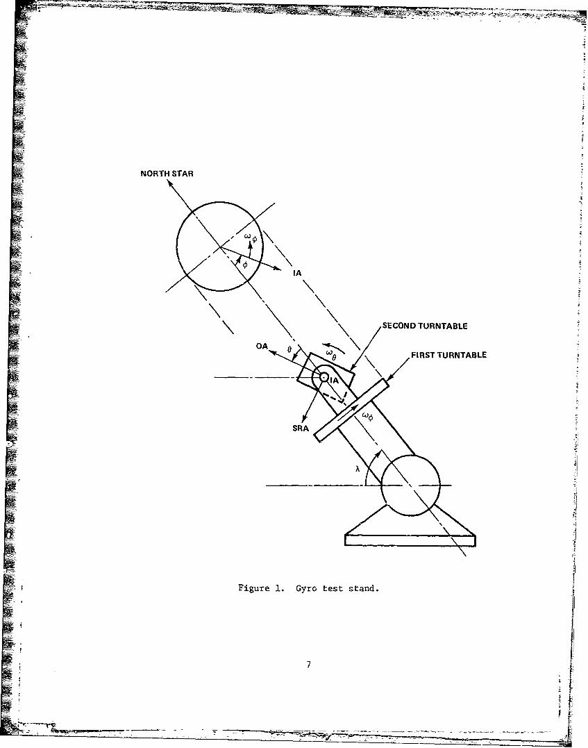
Figure 1 shows a gyro test stand. The stand has two rotatableaxes which are perpendicular to each other. The gyro under test ismounted on the second turntable with its input axis (IA) preciselyaligned to the table axis; therefore, the gyro can be made to tumbleabout two axes. In Figure 1, SRA and OA indicate direction of spinreference axis and output axis, respectively.

The test is performed with the table axis positioned parallel tothe earth rotational axis. The first table axis is elevated to thelocal latitude angle A from the horizontal plane. Under this condition,IA is perpendicular to polar axis and the gyro will not sense the earthrat 2.

Let the first table be rotated at an angular rate w and the second

table be rotated about the IA axis at an angular rate w8 . The gyro

senses oe but not w . Let wR be the gyrn output. Because we is known,

the difference between wR and we, which is the total drift, can be

calculated. In equation form,

D w R -(5)

To avoid the earth rate effect which may be caused by imperfect align-ment of the table axis to the polar axis, it is desirable to turn thetable at a rate approximately ten to twenty times faster than the earth

6

!:---

NORTH STAR

IA

SECOND TURNTABLE

0 FIRST TURNTABLE

IAI

Figure 1. Gyro test stand.

771

rate. To have a good frequency separation property for the driftsignal, which will be discussed later, the rotation rate of the secondaxis should be approximately five times that of the table axis. Areasonable data taking interval is everyt 4o .%ofthe second axis %.rotation. More data points allow a better statistical data reduction.The required data record covers a full rotation of the first axis, orone of its integer multiples.

The remaining problem is the determination of nine drift parametersfrom the measured values of D by means of computer data processing.

IV. DATA PROCESSING ALGORITHM

A. The Measuremeit Equation

Equation (4) shows that eight of the nine drift terms aredependent on either components of acceleration or on their produc.s.Because the test stand is stationary, the acceleration components experi-enced by the gyro are due to earth gravitation. The value of each accel-eration component, in turn, depends on the angular positions of the firstand second table axes. These angular positions are represented by4 and 8 as shown in Figure 1 where their references of measurement arealso indicated.

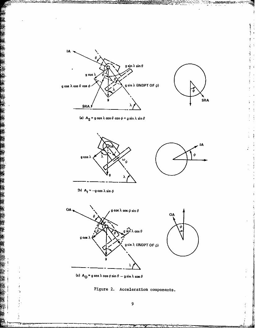
The acceleration components experienced by the gyro can be obtainedwith the help of Figure 2. The accelerations along the spin referenceaxis, input axis, and output axis are given, respectively, by

a. = g cos A cos cos 6 + g sin X sin 8 (6)

ai = -g cos A sin (7)

a = g cos X cos 4sin 6 - g sin X cos 6 (8)

where g is the earth gravitation. Let

8 wt (9)

S¢ t (10)

8

{j

JSR

(a)~~~~ A~cscscs sin Xsin 0

% %

SRQA

IA

c) Al - o i

0 OA

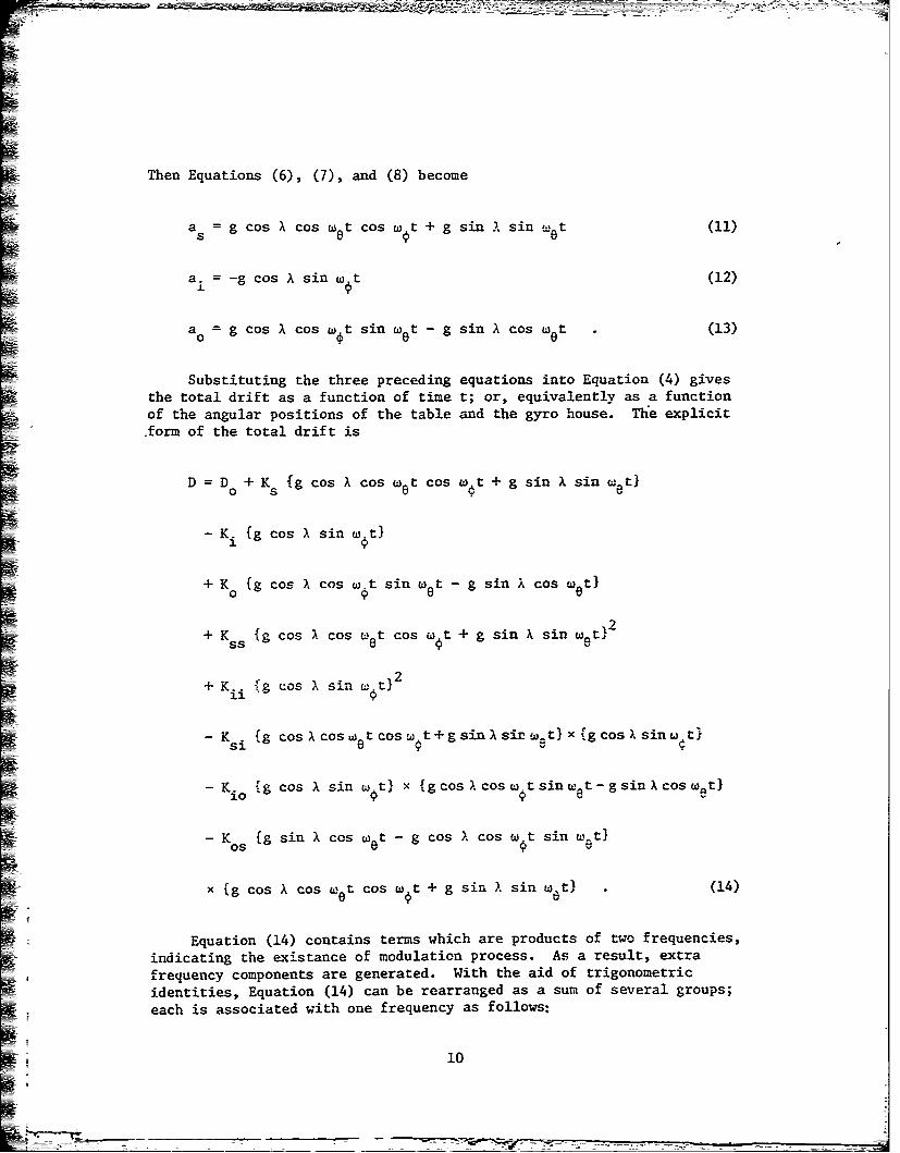
Then Equations (6), (7), and (8) become

a =g cos X cos W t cos Wt + g sin A sin w t (11)

a. = -g cos X sin w t (12)

a° g cos X cos Wt sin w - g sin X cos w t (13)

Substituting the three preceding equations into Equation (4) givesthe total drift as a function of time t; or, equivalently as a function

of the angular positions of the table and the gyro house. The explicit.form of the total drift is

D = D + K {g cos A cos c t Cos W t + g sin X sin ,_t}

-l {g cos X sin wt}

+ K {g cos X cosWt sin wt -g sin X cos 6 t}

+ K {g cos X cos Uet cos Wt + g sin X sin w.t

+ Kii {g cos X sin 1wt}

- K {g cosXCos W tcosw t+gsin~sirw-t}_x{gcos .sinwc t}

- K. {g cos A sin W t} {g cos X cos W t sin et-gsincost}

- K {g sin X cos Wet - g cos A cos W t sin wnt)os

x{g cos X cos Wet cos W 6t + g sir. sin Wt} . (14)

Equation (14) contains terms which are products of two frequencies,

indicating the existance of modulation process. As a result, extra

frequency components are generated. With the aid of trigonometric

identities, Equation (14) can be rearranged as a sum of several groups;

each is associated with one frequency as follows:

10

Do = s (D +K - D) + K.jD1] [K D4 sin w t]

+ (K8 Ss K iiD 1) cos 2

k DD 1+ [K 2sin (w, 2w ~)t -0 K Cos (W -w

2 K. 2 -]

[KsD 5 s in w t - KD 5COS W 6t]

+ [(Ks D4 + Ks, D)COS(W0 + + ) (K _+ K D3 sin(w0 + W)t

+ LKi 0 DI 1 sw + 2w )t -K. Di~ 2w )t]2 i2 slew

+[K ss cos 2(w 0 - )t + K os4sipa 2(w0 - W)]

+ [Kss sin (2w0 + )t K Cos(2w 0 + w)t2 05 2 Os

[Ks 2 - D 2 )w +o 2wet + Ko C 2)w +i 2t] (5

D D3 2

+ [K sin (2 t-K cs(w+W)

3 s 2 eo

155

D, D1

+ ~ [K 'o7-s- 4 si-( t+K s4cs2w0W

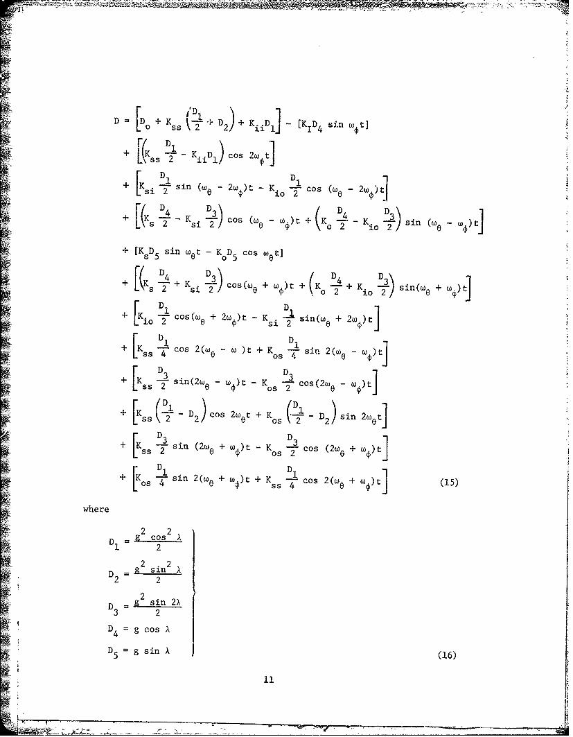
Equation (15) is the measurement equation sought. The equation relatesthe total drift D to drift parameters which are D and K's. It is noted

0that the totai drift contains thirteen different frequency components.The right-hand side of the equation is arranged into thirteen terms; eachterm gives one frequency component.

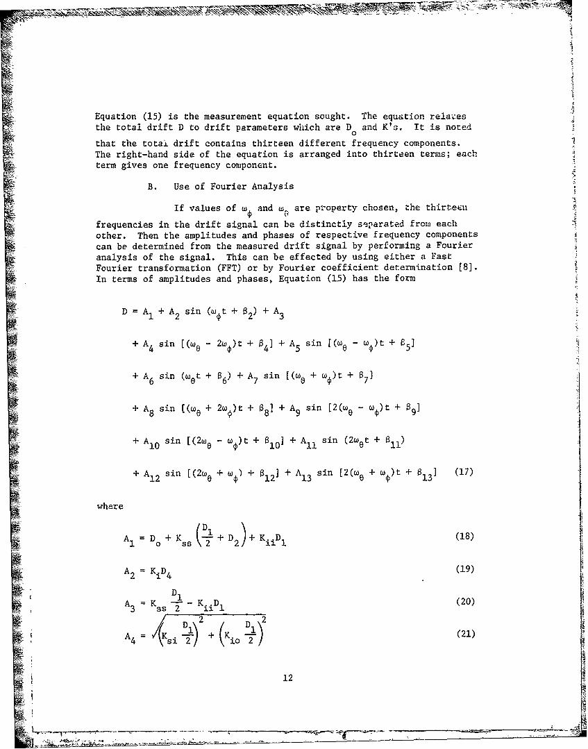
B. Use of Fourier Analysis

If values of w and w are property chosen, the thirteen

frequencies in the drift signal can be distinctly separated from eachother. Then the amplitudes and phases of respective frequency componentscan be determined from the measured drift signal by performing a Fourieranalysis of the signal. This can be effected by using either a FastFourier transformation (FFT) or by Fourier coefficient determination [8].In terms of amplitudes and phases, Equation (15) has the form

D A + A sin (At + + A1 2 si ( t+ 2 ) 3

+ A sin [(w - )t + a + A sin [(w - )t +

[(4 2) 41 A5 [50 w) ~

" A6 sin (wet + a6) + A7 sin [(we + W )t + 071

+ A8 sin ((w + 2w)t + 08] + A9 sin -2(w a W)t + 09]

+ A1 0 sin [(2w - w)t + a00] + A11 sin (2w t + O1)

" A12 sin [(2w0 + Wi) + 012 ] + A1 3 sin [2(w + W )t + 813] (17)

where

A, D + D (18)1 o ss Kii 1

A =KD (19)2 i 4

-- 1K D (20)

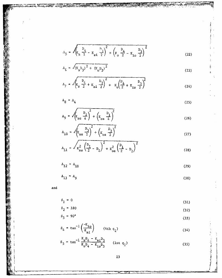
D D 2 / l 2A I + (Kio _ (21)

12

- --4

-

A~ 21D

AD 4A (25)

/i 2~ D 2 i (2

2 2A .K )+ (K /27

D Ds 2

A1 AK 4+ (.i - + K5 T( K -D2 (28)

A1 8 A14 (29)

02 2 182( 2

)D K Ds0 5an 4 s 426

K D DK D

a 0 (35)

-KI10I

ta (4th-

86= tan K (4th ql) (36)

= ta- S A3 (st ql) (37)7 KoD + K ioD 3

a8 = tan-1 ( Ki) (2nd q,) (38)\ K~si

89 = tan-, (I (1st q1) (39)os

-Kos -

aIo = tan-1 -Ks (4th ql) (40)

811 = tan () (1st q,) (41)Os

812 tan Ks (4th ql) (4-)

ss

-83 tan 1 ( (st q1) (43)Os

The parentheses following each angle indicate the quadrant of the angle.

Th Equations (18) to (43) consist of a total of twenty-six equations.

They are used to solve for the nine drift coefficients after Ai and Bi,

i = 1, ..., 13, are determined from the Fourier analysis of the driftsignal. There are more equations than unknowns, indicating redundantinformation. Maximum use of the information will minimize the effectof instrument noise on the determination of drift coefficients from theFourier coefficients. The method chosen for reducing the redundantinformation to an unique set of drift coefficients is the well-knownleast square regression [9, 10].

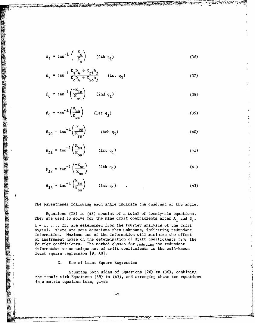
C. Use of Least Square Regression

Squaring both sides of Equations (26) to (30), combiningthe result with Equations (39) to (43), and arranging these ten equationsin a matrix equation form, gives

14

D1 /1

( A .2

D3 ) 1 1

( 2A \2

2!

4 A[

2A 1 30 2

o 1 -cot2 812

22

i-0 1 -tan 2 813

u 2)

i Vector u and matrix M are defined as shown in Equation (44). A well-

known least square regression formula gives [19]

: By taking the square root of Equation (45) and retaining the positivevalues, K and K are determined.

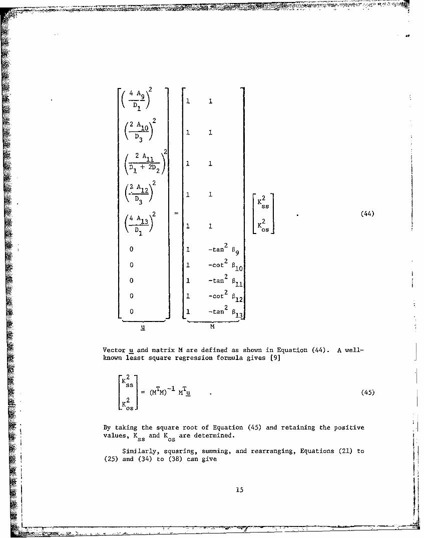
(2)Sim larly, squaring, summing, and rearranging, Equations (21) to

15

0- 1~ -tan -

:!!:::1 ! --m !-~pT

(A) 26 1 0 0]

(~2 r K

_~lL)K 22 2 +A2 D D 2 D22 0 (46)( 5 A 7 ) D4 D4 D3 3 K 2

0 1 -cot 2 a 0~ 0J

2

0 0 0 - tan 4 1

0 0 0 -tan 2 8 1

oD -aD 2 -D 2aD 2

L___ J_ 4 4 3 3v N

where

a tan 5 tan a7 (47)

Vector v and matrix N are defined as shown in Equation (46); the least

square solution for the equation is

K 2S

K2Ko T -1 T=(N N) N V (48)2

Ki

2Ki0j

16

Taking the positive values of the square root of Equation (48) givesKs$ Ko, Ksi , and Kio.

Finally, using Equations (20), (19), and (18) in this order, thefollowing formulas are obtained:

Kss A3K - D1 (49)

A2

K 2 (50)i 4

DO = AI - K (l+D 2)- KiD l (51)

Thus, all nine drift parameters are determined.

D. Discussion

A striking difference between the new and the old two-axis tumble tests is that the former does not require the knowledge ofthe time instant at each data point (or equivalently, the attitude ofthe second axis at each data point). This allows the use of simplertest equipment and demands less operator effort. The conceptual differ-ence is that in the new method the drift parameter identification isperformed using the frequency domain information while in the lattermethod identification is done using the time domain information. Itshould be mentioned that the new method reduces the operator's effortand lessens the test equipment requirement at the expense of a slightlymore complex data procassing algorithm. Because both the new and theold method require a computer for data processing and because the computertime required for either method is insignificant, the trade-off favorsthe new method.

On the other hand, both the new and old two-axis tumble tests have

the following advantages as compared to the other three methods listedin the Introduction. First, there is no need of repeated gyro reposi-tioning which is time-consuming. Second, because both the first andsecond tables are turning at constant speed, there is no motion-inducedtransient effect in the measured drift signal. Third, the measureddrift signal provides sufficient information for the determination ofall nine, rather than partial, drift parameters. Fourth, the required~test time is shorter.

__ Finally, to be truly objective, it should be mentioned chat the old

two-axis tumble test has one advantage over the new method. When usingthe old method, the required data record can be of any length as long as I]it contains at least nine data joints. In other words, the test operator

17

does not have to wait for the table to turn a full revolution althoughthe reduced data record may not provide sufficient redundancy for agood statistical data processing. The algorithm for the old method isincluded as the Appendix for the reader's reference.

V. SIMULATION RESULT

Simulated testing was conducted to demonstrate the proposedmethod. The simulation waa performed with the first table turningabout its axis at twenty times che earth rate and the second tableturning about its axis at 100 times the earth rate. The gyro driftwas simulated. For a full rotation of the table, 864 data points weregenerated.

With the chosen rotation rates for the two tables, the generatedfrequency components in the drift signal are evenly separated by afrequency separation of 20 Hz. Table 1 lists all the frequency components.The amplitudes and tangent of the phases of the frequency components asgenerated by Fourier analysis are shown in Table 2. All nine driftcoefficients resulting from the least square regression are shown inTable 3. The effectiveness of the identification technique and thecorrectness of the data reduction algorithm are demonstrated. Thediscrepancies are evidently due to computation errors, which can bereduced by using the double precision computation. However, the identi-fication accuracy as shown in Table 3 is sufficient for most applications.

VI. CONCLUSION

A frequency domain technique for the identification of gyrodrift coefficients has been developed. The technique involves atwo-axis tumble test and an unique data reduction. Compared to othertechniques, this technique has the merit of providing more completedata for describing gyro drift characteristics. In addition, therequired procedure for testing and data reduction can be convenientlyimplemented into an automated gyro drift coefficient identificationsystem.

A simulation was performed. The result demonstrated the effective-ness of the gyro drift coefficient determination technique and thecorrectness of the data reduction algorithm.

18

il -

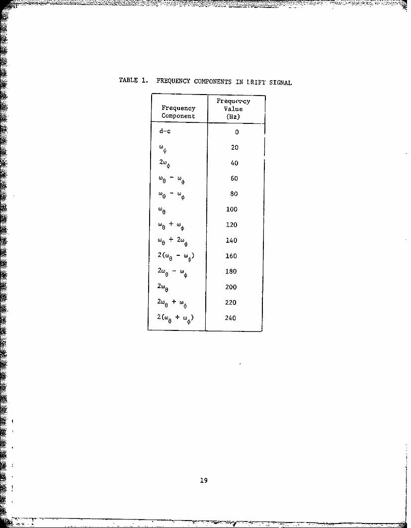
TABLE 1. FREQUENCY COMPONENTS IN 1)RIFT SIGNAL

Frequei'cyFrequency ValueComponent (Hz)

d-c 0

w 20

2w 40

w - 60

w w 80

we 100

O + w¢ 120

w + 2w€ 140

2(w w) 160

2 w w 1800

2wO 200

2 w + we 220

2 (w + w) 240

#-:i

1 19

-4- - - 7-- * -~- -- ~- - A

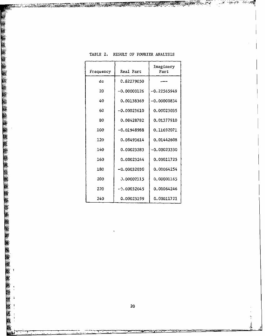
TABLE 2. RESULT OF FOURIER ANALYSIS

Imagin~aryFrequency Real Part Part

de ~0.82279050 -

20 -0.00000126 -0.22565949

40 0.00138369 -0.00000834

60 -0.00023610 0.00023035

80 0.08428782 0.01377910

100 -0.01948988 0.11692071

120 0.08493614 0.01442608

140 0.00023283 -0.00023330

160 0.00023244 0. 00011725

180 -0.00032030 0.00064254

200 3.00002115 0. 00001165

220 -Q'.00032045 0.00064246

240 0.00023199 0.00011721

20

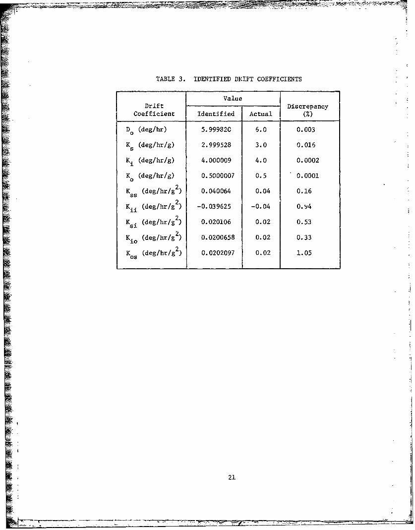
TABLE 3. IDENTIFIED DRIFT COEFFICIENTS

IValueDrift TDiscrepancyCoefficient Identified Actual (%)

S0 (deg/hr) 5.99982C 6.0 0.003

Ks (deg/hr/g) 2.999528 3.0 0.016

K. (deg/hr/g) 4.000009 4.0 0.0002

K 0 (deg/hr/g) 0.5000007 0.5 0.0001

K (deg/hr/g2) 0.040064 0.04 0.16

ii (deglhr/g ) -0.039625 -0.04 0.94

Ksi (deg/hr/g 2) 0.020106 0.02 0.53

K. (deg/hrg 2) 0.0200658 0.02 0.33

2K (deg/hr/g2) 0.0202097 0.02 1.05Os

21- -,

-Pt-- - -1111:i -

REFERENCES

1. Pitman, G. R., Jr., Editor, Inertial Guidance, New York: John-Wileyand Sons, Inc., 1962.

2. Russell, J. F., Gyroscope Standard Torque-to-Balance Test,Report 4DC-TR-67-79, Holloman Air Force Base, New Mexico, June 1967.

3. Bonafede, W. J., "Tabe!-Servo Gvro Evaluation," Section 6 of Notesfor Summer 1963 Program 16.39S, Department of Aeronautics andAstronautics, MIT, Cambridge, Massachusetts, 1963.

4. Vaughn, R. S., "Test Methods for the Single Degree of FreedomIntegrating Rate Gyro Phase !I: Acceleration Sensitive DriftCharacteristics," Report No. NADC-AI-6191, US Naval Air DevelopmentCenter, Johnsville, Pennsylvania, December 1961.

5. Johnston, J. V., Analytical Solution for Two-Axis Tumble Test,Report No. RGL-73-11B, US Army Missile Research, Development andEngineering Laboratory, US Army Missile Command, Redstone Arsenal,Alabama, September 1973.

6. Lorenzini, D. A., "Testing of Precision Inertial Gyroscopes,"AGARDograph No. 19Z, Advisory Group for Aerospace Research and-Development, North Atlantic Treaty Organization, April 1973.

7. The Analytic Science Corporation, Reading, Massachusetts,"Dynamic Errors in Strapdown Inertial Navigation Systems,"NASA CR-1962, 1971.

8. Oppenheim, A. V. and Schafer, R. W., Digital Signal Processing,Englewood Cliffs, New Jersey: Prentice-Hall, Inc., 1975.

9. Ralston, A., A First Course in Numerical Analysis, New York:McGraw-Hill Book Co., 1965.

10. Hung, J. C. and White, H. V., "Self-Alignment Techniques forInertial Measurement Units," IEEE Transactions on Aerospaceand Electronic Systems, Volume AES-II, No. 6, November 1975.

IV

23

, r_4 5 _

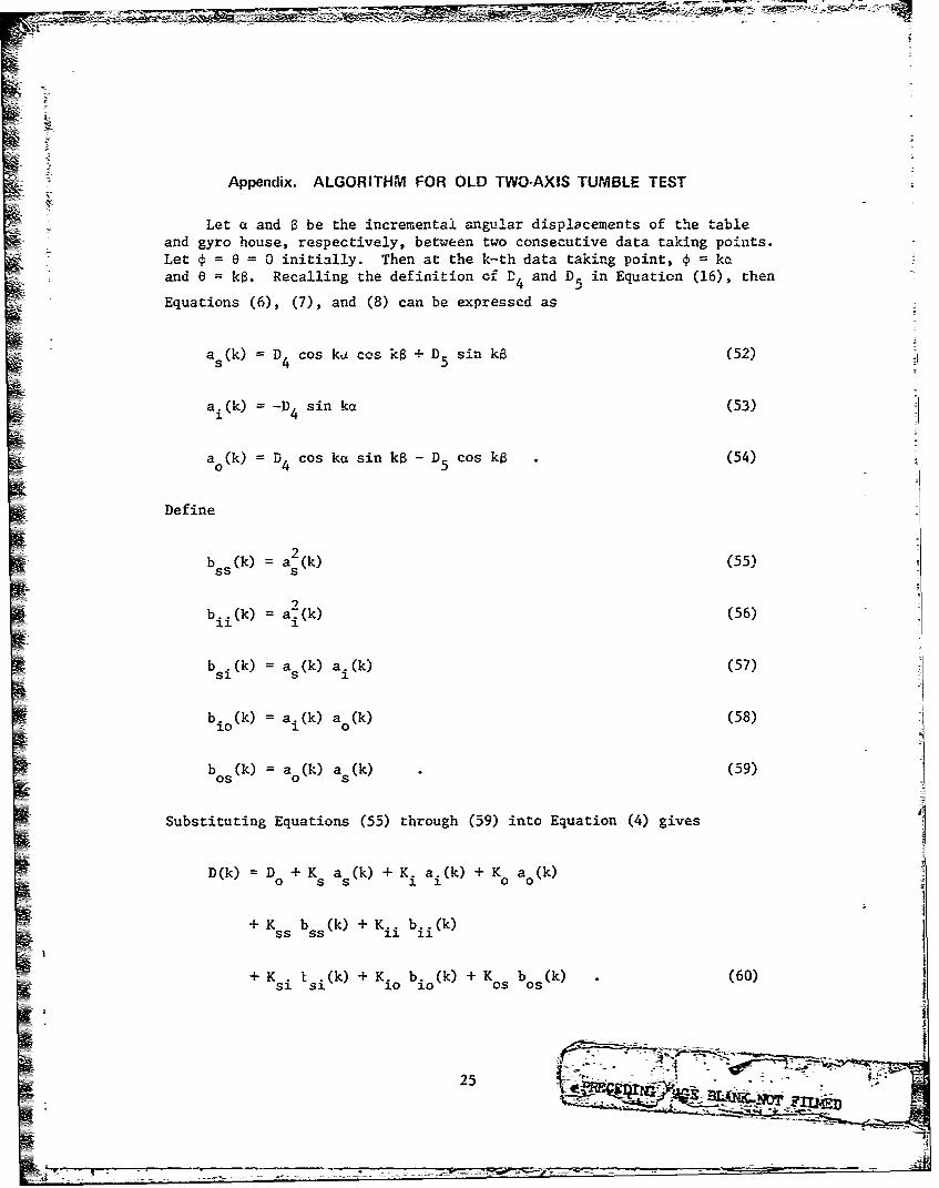
Appendix. ALGORITHM FOR OLD TWO-AXIS TUMBLE TEST

Let a and 0 be the incremental angular displacements of the tableand gyro house, respectively, between two consecutive data taking points.Let =e = 0 initially. Then at the k-th data taking point, k icand e ka. Recalling the definition of D4and D 5 in Equation (16), then

Equations (6), (7), and (8) can be expresscd as

a (k) D cos ka.cs k+ D sin ke (52)s 4

a .(k) -D 4 sin kac (53)

a (k) D4 cos kac sin k8-D 5 cos ka (54)

Define

b (k a(k) (55)ss s

b. (k) a ZkK) (56)

b si(k) as(k) a.(k) (57)

b. MI a.(k) a (k) (58)

b M a (k) a(k) (59)05 0 S

Substituting Equations (55) through (59) into Equation (4) gives

D(k) D + K a (k) + K.i a.i(k) + K a (k)0 5 5 10 0

+K bs (k)+K.. b..(k)

+ K si s () + K io b.i (k) + K osb os(k) (60)IKE,

25 -

L_- -------

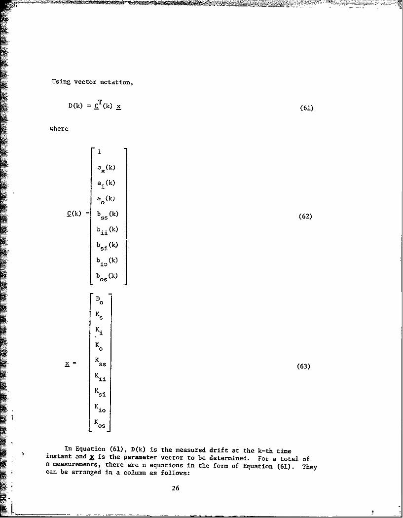
Using vector nctation,

D (k) =C(k) x (61)

where

a (k)

a. (k)ii

b .(k)i

b.s (k)

b io(k)

D0

KS

K .

K0

Kss (63)

K.Si

K.1.0

K

In Eqain(1,Dk is the measured drift at the k-th time Te

instnt nd istheparameter vector to be determined. For a total of

canbe rragedin coumnas follows:

D(1) c(

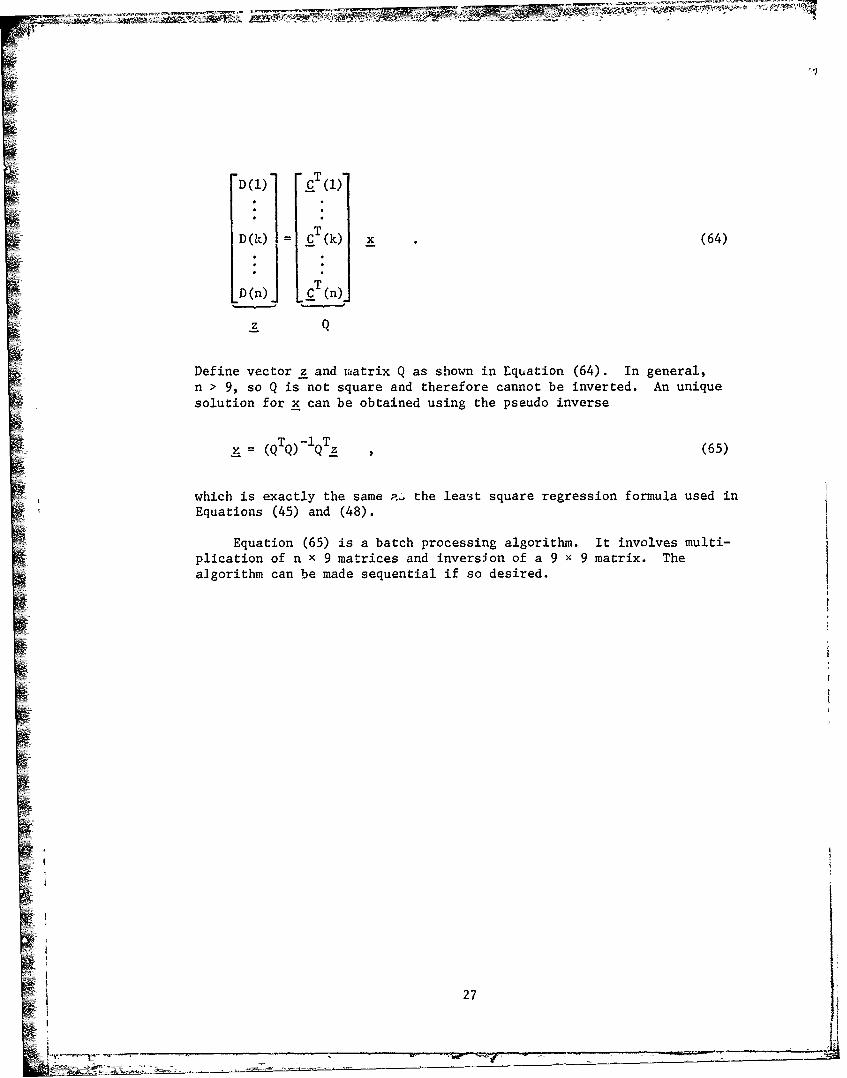
D(k) = cT(k) x . (64)

D (n) CT (n)_

z Q

Define vector z and matrix Q as shown in Equation (64). In general,n > 9, so Q is not square and therefore cannot be inverted. An uniquesolution for x can be obtained using the pseudo inverse

(QTQ)-lQT z (65)

which is exactly the same P. the lea'st square regression formula used inEquations (45) and (48).

Equation (65) is a batch processing algorithm. It involves multi-plication of n x 9 matrices and inversion of a 9 × 9 matrix. Thealgorithm can be made sequential if so desired.

27

-~~~ -- 7~ --- 4

DISTRIBUTION

No. of Copies

Defense Documentation CenterCameron StationAlexandria, Virginia 22314 12

Commander

US Army Materiel Development and Readiness CommandATTN: DRCRD 1

DRCDL 15001 Eisenhower AvenueAlexandria, Virginia 22333

DRSMI-FR, Mr. Strickland 1-LP, Mr. Voigt 1-R, Dr. McDaniel 1

Dr. Kobler 1-RBD 3-RPR (Record Set) 1

(Reference Copy) 1

28