TECHNICAL REPORT NO. TR-2015-04

JANUARY 2015

US ARMY MATERIEL SYSTEMS ANALYSIS ACTIVITY

ABERDEEN PROVING GROUND, MARYLAND 21005-5071

DISTRIBUTION A: APPROVED FOR PUBLIC RELEASE; DISTRIBUTION IS UNLIMITED.

IAW Memorandum, Secretary of Defense, 27 December 2010, Subject: Consideration of Costs in DoD Decision-Making, the cost of the study resulting in this report is $205,000.

SCHEDULE RISK EVENT DRIVEN METHODOLOGY (SREDM): FY13 ARMY STUDIES PROGRAM

PROJECT FINDINGS

DISCLAIMER

The findings in this report are not to be construed as an official Department of the Army position unless so specified by other official documentation.

WARNING

Information and data contained in this document are based on the input available at the time of preparation.

TRADE NAMES

The use of trade names in this report does not constitute an official endorsement or approval of the use of such commercial hardware or software. The report may not be cited for purposes of advertisement.

REPORT DOCUMENTATION PAGE Form Approved

OMB No. 0704-0188 Public reporting burden for this collection of information is estimated to average 1 hour per response, including the time for reviewing instructions, searching existing data sources, gathering and maintaining the data needed, and completing and reviewing this collection of information. Send comments regarding this burden estimate or any other aspect of this collection of information, including suggestions for reducing this burden to Department of Defense, Washington Headquarters Services, Directorate for Information Operations and Reports (0704-0188), 1215 Jefferson Davis Highway, Suite 1204, Arlington, VA 22202-4302. Respondents should be aware that notwithstanding any other provision of law, no person shall be subject to any penalty for failing to comply with a collection of information if it does not display a currently valid OMB control number. PLEASE DO NOT RETURN YOUR FORM TO THE ABOVE ADDRESS. 1. REPORT DATE (DD-MM-YYYY) January 2015

2. REPORT TYPE Technical Report

3. DATES COVERED (From - To)

4. TITLE AND SUBTITLE SCHEDULE RISK EVENT DRIVEN METHODOLOGY (SREDM): FY13 ARMY STUDIES PROGRAM PROJECT FINDINGS

5a. CONTRACT NUMBER 5b. GRANT NUMBER 5c. PROGRAM ELEMENT NUMBER

6. AUTHOR(S) Timothy Biscoe, Andrew Clark, John Nierwinski

5d. PROJECT NUMBER 5e. TASK NUMBER 5f. WORK UNIT NUMBER 7. PERFORMING ORGANIZATION NAME(S) AND ADDRESS(ES)

Director US Army Materiel Systems Analysis Activity 392 Hopkins Road Aberdeen Proving Ground, MD

8. PERFORMING ORGANIZATION REPORT NUMBER

TR-2015-04

9. SPONSORING / MONITORING AGENCY NAME(S) AND ADDRESS(ES) 10. SPONSOR/MONITOR’S ACRONYM(S)

11. SPONSOR/MONITOR’S REPORT NUMBER(S)

12. DISTRIBUTION / AVAILABILITY STATEMENT DISTRIBUTION A: APPROVED FOR PUBLIC RELEASE; DISTRIBUTION IS UNLIMITED. 13. SUPPLEMENTARY NOTES 14. ABSTRACT AMSAA conducts independent schedule risk assessments to support Analysis of Alternatives (AoAs). AMSAA’s current approach, Schedule Risk Data Decision Methodology (SRDDM), is predicated upon historical phase level analysis. As part of an Army Studies Program funded effort, AMSAA set out to enhance their schedule risk methodology through historical event level analysis. AMSAA developed a preliminary Schedule Risk Event Driven Methodology (SREDM) that utilizes historical event level data to determine a probability of phase completion within the scheduled time provided by the Program Manager (PM). A case study was performed using event data to demonstrate the feasibility of applying SREDM to an AoA. Future research topics include selecting analogous data and technical risk assessment integration. 15. SUBJECT TERMS analysis of alternatives, AMSAA, acquisition, schedule, risk, assessment, analysis,

16. SECURITY CLASSIFICATION OF: 17. LIMITATION OF ABSTRACT

18. NUMBER OF PAGES

19a. NAME OF RESPONSIBLE PERSON Timothy E. Biscoe

a. REPORT UNCLASSIFIED

b. ABSTRACT UNCLASSIFIED

c. THIS PAGE UNCLASSIFIED

SAME AS REPORT

53

19b. TELEPHONE NUMBER (include area code) 410-278-0403 Standard Form 298 (Rev. 8-98)

Prescribed by ANSI Std. Z39.18

i

THIS PAGE INTENTIONALLY LEFT BLANK.

ii

CONTENTS Page

LIST OF FIGURES ......................................................................................................... v LIST OF TABLES .......................................................................................................... vi ACKNOWLEDGEMENTS .......................................................................................... vii LIST OF ACRONYMS ............................................................................................... viii

1. INTRODUCTION ........................................................................................................... 1

1.1 Background. ......................................................................................................... 1 1.2 Schedule Risk Assessment Overview. ................................................................. 1

1.2.1 Objective Assessments. ............................................................................ 2 1.2.2 Risk Assessment Customers. .................................................................... 2 1.2.3 Risk Assessment Methodology Constraints and Influential Factors. ....... 2 1.2.4 Current Schedule Risk Assessment Methodology - SRDDM. ................. 3 1.2.5 Methodology Enhancement Effort - SREDM. ......................................... 3 1.2.6 SRDDM and SREDM – Advantages and Disadvantages. ....................... 4

2. REVIEW OF SRDDM ..................................................................................................... 5

2.1 Introduction and Background. .............................................................................. 5 2.2 SRDDM Methodology and Coverage Validation. ............................................... 5 2.3 Application. .......................................................................................................... 6

3. SREDM METHODOLOGY ............................................................................................ 7

3.1 Introduction. ......................................................................................................... 7 3.2 Schedule Risk Modeling Research and Engagements. ........................................ 8

3.2.1 Engagements with DoD Acquisition Community. ................................... 8 3.2.2 Schedule Model Implementation. ........................................................... 10 3.2.3 SME Elicitation. ..................................................................................... 11

3.3 Data Collection................................................................................................... 13 3.3.1 Phase Level Data. ................................................................................... 13 3.3.2 Event Level Data. ................................................................................... 13 3.3.3 Analogous Data Assumption.. ................................................................ 14 3.3.4 Technical Risk Data. .............................................................................. 16 3.3.5 Sources. .................................................................................................. 16 3.3.6 Event Level Data Collection Process.. ................................................... 18

3.4 Case Study Schedule Models. ............................................................................ 21 3.4.1 Discussion of Model Types. ................................................................... 21 3.4.2 SREDM Schedule Model 1.. .................................................................. 23 3.4.3 SREDM Schedule Model Excursions.. .................................................. 25 3.4.4 SREDM Schedule Model 1 Input Data. ................................................. 27 3.4.5 SREDM Schedule Model 1 Monte Carlo Simulation. ........................... 28 3.4.6 SREDM Schedule Model 1 Monte Carlo Input Data.. ........................... 28 3.4.7 SREDM Schedule Model 1 Monte Carlo Logic.. .................................. 29 3.4.8 SREDM Schedule Model 2. ................................................................... 30 3.4.9 SREDM Schedule Model 3.. .................................................................. 31 3.4.10 SREDM Schedule Model Summary.. ................................................... 33

iii

CONTENTS Page

4. VERIFICATION AND VALIDATION (V&V) PLAN ................................................ 35 5. CONCLUSION .............................................................................................................. 36

5.1 Path Forward. ..................................................................................................... 36 REFERENCES ........................................................................................................................... 37 APPENDIX A – DISTRIBUTION LIST ................................................................................ A-1

iv

LIST OF FIGURES

Figure No.

Title Page

Figure 1. SRDDM and SREDM - Advantages and Disadvantages Summary. .............................. 4 Figure 2. Notional Schedule Risk Assessment Results. ................................................................. 6 Figure 3. SREDM Initial Conceptualization. ................................................................................. 7 Figure 4. Example of SAR Schedule Summary Table with Change Explanations. .................... 17 Figure 5. Example of Summary-Level Schedule. ........................................................................ 18 Figure 6. Example of Historical Event Date Spreadsheet Log. ................................................... 18 Figure 7. Example of Historical Milestone Delay Tracking. ....................................................... 19 Figure 8. Example of Event Schedule Network Diagramming.................................................... 20 Figure 9. Summary Level Schedule. ............................................................................................ 21 Figure 10. Summary Level Schedule with Event Modeling Network. ........................................ 22 Figure 11. Network Model and Data Availability. ...................................................................... 23 Figure 12. Updated Network Model based on Data Availability................................................. 24 Figure 13. Aggregated Network Model: Schedule Model 1 – Level 3 ........................................ 24 Figure 14. Aggregated Network Model: Schedule Model 1 – Level 2. ....................................... 26 Figure 15. Aggregated Network Model: Schedule Model 1 – Level 1 ........................................ 26 Figure 16. Schedule Model 2: Delay Modeling Macro-view. ..................................................... 30 Figure 17. Schedule Model 2: Calculating Non-delay Phase Completion Durations. ................. 31 Figure 18. Schedule Model 2: Delay Modeling Micro-view. ..................................................... 31 Figure 19. Schedule Model 3: KT Development Modeling – Macro-view. ................................ 32 Figure 20. Schedule Model 3: KT Development Modeling – Micro-view. ................................. 32 Figure 21. Visual Summary of SREDM Model Completion Time Distributions........................ 33

v

LIST OF TABLES

Table No.

Title Page

Table 1. Notional Historical Event Level Duration Summary. .................................................... 20 Table 2. Summary of SREDM Models. ....................................................................................... 34

vi

ACKNOWLEDGEMENTS

The US Army Materiel Systems Analysis Activity (AMSAA) recognizes the following individuals for their contributions to this report. The author(s) are: Timothy Biscoe, Logistics Analysis Division, LAD Andrew Clark, Weapon Systems Analysis Division, WSAD John Nierwinski, Weapon Systems Analysis Division, WSAD The authors wish to acknowledge the contributions of the following individuals for their assistance in the creation and review of this report:

Robert Chandler, Weapon Systems Analysis Division, WSAD Jennifer Forsythe, Weapon Systems Analysis Division, WSAD Kevin Guite, Weapon Systems Analysis Division, WSAD Suzanne Singleton, Weapon Systems Analysis Division, WSAD George Steiger, Weapon Systems Analysis Division, WSAD Randolph Wheeler, Weapon Systems Analysis Division, WSAD

vii

LIST OF ACRONYMS AAS - Armed Aerial Scout ACAT - Acquisition Category ADSS - ATEC Decision Support System AMPV - Armored Multi-Purpose Vehicle AMSAA - US Army Materiel Systems Analysis Activity AoA - Analysis of Alternatives ATEC - Army Test and Evaluation Command BC - Bias Corrected CDR - Critical Design Review CI - Confidence Interval DASC - Department of the Army Systems Coordinator DAMIR - Defense Acquisition Management Information Retrieval DoD - Department of Defense DTIC - Defense Technical Information Center EMD - Engineering and Manufacturing Development FRP - Full-Rate Production FUE - First Unit Equipped FY13 - Fiscal Year 2013 GAO - US Government Accountability Office GCV - Ground Combat Vehicle IFPC - Indirect Fire Protection Capability IMS - Integrated Master Schedule IOC - Initial Operational Capability IOTE - Initial Operational Test and Evaluation IPT - Integrated Product Team IRL - Integration Readiness Level KT - Key Technology LCB - Lower Confidence Bounds LFT&E - Live Fire Test and Evaluation LRIP - Low Rate Initial Production LUT - Limited User Test MDAP - Major Defense Acquisition Program MRL - Manufacturing Readiness Level

viii

MS - Milestone NAVAIR - U.S. Navy Naval Air Systems Command ODASA-CE - Office of the Deputy Assistant Secretary of the Army for Cost & Economics OSD-CAPE - Office of the Secretary of Defense for Cost and Program Evaluation P&D - Production and Deployment PDR - Preliminary Design Review PEO - Program Executive Office PM - Program Manager PQT - Production Qualification Test PVT - Production Verification Test RDDS - Research Development and Descriptive Summaries RFP - Request for Proposal SAR - Selected Acquisition Report SME - Subject Matter Expert SRDDM - Schedule Risk Data Decision Methodology SREDM - Schedule Risk Event Driven Methodology TDS - Technology Development Strategy TEMP - Test and Evaluation Master Plan TR - Technical Report TRL - Technology Readiness Level WBS - Work Breakdown Structure WSARA - Weapons Systems Acquisition Reform Act

ix

SCHEDULE RISK EVENT DRIVEN METHODOLOGY (SREDM): FY13 ARMY STUDIES PROGRAM PROJECT FINDINGS

1. INTRODUCTION 1.1 Background. A prevalent challenge currently facing the United States Army and government as a whole are budgetary reductions. More than ever, Army leaders need to make informed acquisition decisions that reflect wise stewardship of sparse federal dollars and ensure the current and future needs of the Warfighter are met. Under Secretary of Defense, Acquisition, Technology, and Logistics, the Honorable Frank Kendall is currently leading the charge for making more informed acquisition decisions. Kendall recently stated, “Value obtained in acquisition is a balance of costs, benefits, and prudent risks. Risks are a fact of life in acquiring the kinds of products our warfighters need, and these risks must be objectively managed” (Performance of the Defense Acquisition System, 2013) [Reference 1]. An accurate and independent acquisition schedule risk assessment for a set of materiel alternatives is a key input to making risk-informed decisions. The Weapon Systems Acquisition Reform Act (WSARA) of 2009 [Reference 2] is driving more analysis to support the Analysis of Alternatives (AoA), to include risk assessments and trades among cost, schedule, and performance. Cost risk assessment methodology was developed by the Office of the Deputy Assistant Secretary of the Army for Cost & Economics (ODASA-CE). The cost risk assessment methodology is documented in a draft US Army Cost Analysis Handbook. Army Materiel Systems Analysis Activity (AMSAA), in response to WSARA, led an Army Risk Integrated Product Team (IPT) that was formed in March 2011 at the direction of Army leadership to develop repeatable and quantitative methodologies for conducting independent technical, schedule, and cost risk assessments to support acquisition studies. In October 2011, AMSAA established a permanent Risk Team to meet risk assessment demands. The Schedule Risk Data Decision Methodology (SRDDM) and Technical Risk Methodology have been significant achievements developed through the combined efforts of the Risk IPT and AMSAA Risk Team. As part of a Fiscal Year 2013 (FY13) Army Studies Program initiative, the Risk Team sought out potential enhancements to their existing methodologies through the research and development of a Schedule Risk Event Driven Methodology (SREDM). The SREDM initiative illuminated critical program events and key aspects that create risk within schedule. SREDM research and development has opened the door for schedule current and future schedule risk assessment advancements. 1.2 Schedule Risk Assessment Overview. Risk, defined in the context of Department of Defense (DoD) acquisition, is a measure of future uncertainties in achieving program performance goals and objectives within defined cost, schedule, and performance constraints. Acquisition risk assessments are part of an overall risk management process in which a program’s risk exposure is determined. Acquisition decisions need to be made despite the future outcomes of these decisions being highly uncertain. Risk assessments provide a means to help measure uncertainty and assist in making risk-informed decisions. As a facet of acquisition risk analysis, schedule risk assessments use quantitative and qualitative techniques to measure the likelihood and confidence in meeting a program’s estimated schedule.

1

1.2.1 Objective Assessments. A key feature of AMSAA’s risk assessments are that they are independently generated. AMSAA is one of the Army’s providers of objective and independent analyses. AMSAA is an independent analysis organization because it is not under the management of a program office directly responsible for carrying out the acquisition of the program and is not involved in the development of technologies related to the program. This helps to mitigate the effects of biases such as an over optimism bias, which could creep into estimates prepared by advocates of the acquisition program [Reference 4].

1.2.2 Risk Assessment Customers. The primary customer of AMSAA’s independent risk assessments is the Office of the Secretary of Defense for Cost Assessment and Program Evaluation (OSD-CAPE). OSD-CAPE issues the AoA study guidance and assesses whether the AoA report is sufficient to inform acquisition decisions. The risk assessments inform the program office acquisition strategies and their risk management process.

1.2.3 Risk Assessment Methodology Constraints and Influential Factors. The objective of the risk assessment process is to measure the risk exposure within each program alternative being considered. A risk assessment method for an AoA should be developed within the following set of constraints:

- Must be repeatable - Must be consistent among similar AoAs - Must have the ability to execute within a timeframe allowed per AoA guidance - Must limit bias through objective and independent evaluations - Must be formal, systematic, and applied in a disciplined manner within the

organization; in other words, institutionalized - Methods and results should have the ability to be clearly understood and

communicated to all key stakeholders involved.

The following list of acquisition risk assessment factors should be considered during data collection and modeling efforts. These factors can influence the constraints, the ability to meet the decision maker’s needs, and the overall results of the risk assessment:

- Availability of historical data - Availability of data on the proposed program at the time of an AoA - Characteristics that make one program or system more complex or similar than

another [e.g., system type, system capabilities, acquisition strategy, acquisition category (ACAT), interfaces, key technology maturity levels]

- Ability to support ACAT I, II, and III risk assessments - Ability to integrate technical, performance, and cost risk assessments - Ability to support trade analysis (e.g. trade technologies, performance capabilities,

costs, schedule, and risks to decide best materiel solution) - Ability to utilize Subject Matter Expert (SME) data - Model complexity/simplicity - Model predictability, supportability, and usability

2

1.2.4 Current Schedule Risk Assessment Methodology - SRDDM. AMSAA utilizes SRDDM [Reference 5], developed in 2012, to conduct independent schedule risk assessments. SRDDM utilizes historical defense acquisition system phase level (e.g., Engineering and Manufacturing Development (EMD) phase, Production and Deployment (P&D) phase) durations from analogous programs in order to assess a probability, along with a confidence interval, of meeting the Program Manager’s (PM) schedule. Analogous acquisition programs are historical programs or elements of historical programs exhibiting characteristics that are relatively similar to a specific AoA alternative. Some of these characteristics include program type, acquisition strategy, system capabilities, critical technologies, and additional schedule drivers. In this methodology, a low probability indicates an unfavorable outcome or high risk. Another feature of SRDDM is its ability to examine how risk changes as the PM schedule changes.

1.2.5 Methodology Enhancement Effort - SREDM. To supplement SRDDM, AMSAA to developed an initial version of SREDM in FY13 through the Army Studies Program. The goal of the effort was to enhance the current methodology such that risk assessments could be performed by analyzing historical and analogous event level dates to determine the probability of meeting the PM’s schedule. An event can be thought of as any defined point within a program’s development schedule. For example, some historical events that were researched included reviews like Preliminary Design Review (PDR) or Critical Design Review (CDR), start and end points of major tests like the Production Qualification Test (PQT) or Production Verification Test (PVT), contracting landmarks like Request for Proposal (RFP) or Contract Awards, product deliveries like the 1st Prototype or 1st Low Rate Initial Production (LRIP) platform, and major milestones or decision points like Milestones A, B, C, or Full Rate Production (FRP) Decision.

3

1.2.6 SRDDM and SREDM – Advantages and Disadvantages. There are advantages and disadvantages to both SRDDM and SREDM for use in an AoA. Figure 1 shows a side-by-side comparison chart of some of each methodology’s advantages and disadvantages. Advantages for one methodology tend to be disadvantages for the other methodology and vice versa. The chart was initially developed to help plan and strategize SREDM research and development efforts.

Figure 1. SRDDM and SREDM - Advantages and Disadvantages Summary.

4

2. REVIEW OF SRDDM 2.1 Introduction and Background. SRDDM begins by determining if enough historical analogous program schedule data exists to utilize quantitative techniques to conduct the schedule risk assessment. Within SRDDM are Monte Carlo simulations and mathematical models that build a confidence interval (CI) around the probability of meeting the PM’s schedule. If the CI width is within the user established tolerance, then enough analogous program schedule data exists to build a schedule distribution. Risk studies are conducted by changing the planned schedule date and examining the sensitivity of the probability of meeting this planned schedule. SRDDM currently has two approach methods (analogous data and ratio referencing), which are discussed in the SRDDM technical report [Reference 3]. AMSAA has applied the SRDDM analogous data method to several recent acquisition studies, which include the following AoAs:

• Indirect Fire Protection Capability (IFPC) • Armored Multi-Purpose Vehicle (AMPV) • Armed Aerial Scout (AAS) • Ground Combat Vehicle (GCV).

The SRDDM ratio referencing method has never been applied due to insufficient data for initial program schedule estimates. The ratio method along with other referencing methods will be explored in the future. 2.2 SRDDM Methodology and Coverage Validation. The SRDDM methodology is composed of many modes (determining if enough data exists, studies assessing risk sensitivity to changes in the PM’s schedule, etc.). The steps utilized within the current SRDDM model (analogous data) are:

• Use the identified analogous schedule data for the specific materiel alternative, compute the probability of meeting the PM’s schedule. This is the percentage of the analogous data that falls below the PM’s schedule; for instance a probability of completing EMD phase of 85% entails that analogous data supports the PM’s schedule, but 15% of the time programs exceeded the proposed schedule.

• Determine if enough data exists to use the estimated probability. A CI is then built for meeting the PM’s schedule using the analogous data.

• To build this CI, one of three CI methods are utilized depending on the number of analogous programs and the suspected probability of meeting the PM’s schedule. These are called: Monte Carlo Simulation Percentile Method Monte Carlo Simulation Bias Corrected (BC) Method Wilson Score Interval

• After using one of these three methods to build a CI, errors (CI width) are examined. The lower confidence bound (LCB) is of most concern because the LCB represents a higher risk.

5

In order to accurately build a 2-sided CI stochastic model, enough sample data is needed to achieve the requested level of confidence (e.g., 90%). Coverage models are used to validate the model accuracy. Coverage is defined to be the percentage of CI’s that contain the true population parameter P, where each CI is constructed with some method at some confidence level for a given random sample of n analogous programs. In other words, the inference method (Monte Carlo simulation with BC method) must be run 500+ times (500+ samples drawn from a parametric or nonparametric population) to obtain 500+ CI’s. These 500+ samples are not to be confused with the 500+ iterations from the Monte Carlo simulation with BC method. Inspection is made to determine how many CI’s contain the true P [Reference 3]. Accuracy is defined to be how close the coverage is to the requested level of confidence – the closer it is, the more accurate the model. Lessons learned from a coverage validation study revealed the following results:

• At least 6 analogous programs (n) are needed to perform the Wilson Score Interval. • If the probability is extreme (near 0 or 1) then always use the Wilson Score Interval. • If the probability is not extreme, then use one of the two Monte Carlo methods:

Percentile Method if 10 < n < 17. Bias Correction Method if n > 17.

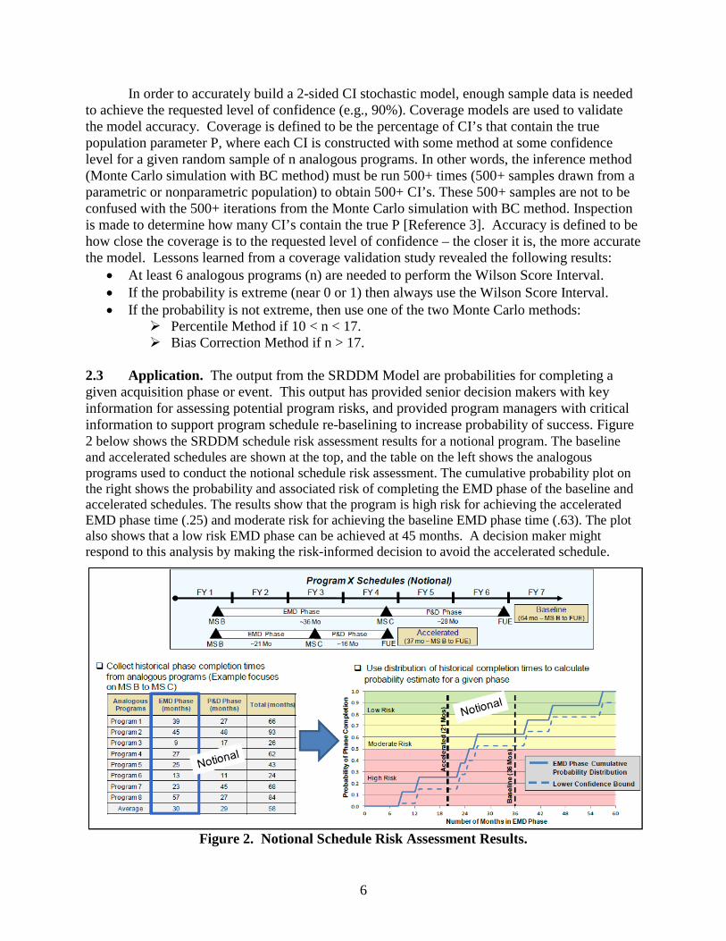
2.3 Application. The output from the SRDDM Model are probabilities for completing a given acquisition phase or event. This output has provided senior decision makers with key information for assessing potential program risks, and provided program managers with critical information to support program schedule re-baselining to increase probability of success. Figure 2 below shows the SRDDM schedule risk assessment results for a notional program. The baseline and accelerated schedules are shown at the top, and the table on the left shows the analogous programs used to conduct the notional schedule risk assessment. The cumulative probability plot on the right shows the probability and associated risk of completing the EMD phase of the baseline and accelerated schedules. The results show that the program is high risk for achieving the accelerated EMD phase time (.25) and moderate risk for achieving the baseline EMD phase time (.63). The plot also shows that a low risk EMD phase can be achieved at 45 months. A decision maker might respond to this analysis by making the risk-informed decision to avoid the accelerated schedule.

Figure 2. Notional Schedule Risk Assessment Results.

6

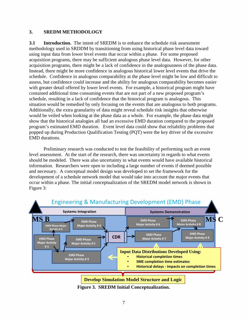
3. SREDM METHODOLOGY 3.1 Introduction. The intent of SREDM is to enhance the schedule risk assessment methodology used in SRDDM by transitioning from using historical phase level data toward using input data from lower level events that occur within a phase. For some proposed acquisition programs, there may be sufficient analogous phase level data. However, for other acquisition programs, there might be a lack of confidence in the analogousness of the phase data. Instead, there might be more confidence in analogous historical lower level events that drive the schedule. Confidence in analogous comparability at the phase level might be low and difficult to assess, but confidence could increase and the ability for analogous comparability becomes easier with greater detail offered by lower level events. For example, a historical program might have contained additional time consuming events that are not part of a new proposed program’s schedule, resulting in a lack of confidence that the historical program is analogous. This situation would be remedied by only focusing on the events that are analogous to both programs. Additionally, the extra granularity of data might reveal schedule risk insights that otherwise would be veiled when looking at the phase data as a whole. For example, the phase data might show that the historical analogies all had an excessive EMD duration compared to the proposed program’s estimated EMD duration. Event level data could show that reliability problems that popped up during Production Qualification Testing (PQT) were the key driver of the excessive EMD durations. Preliminary research was conducted to test the feasibility of performing such an event level assessment. At the start of the research, there was uncertainty in regards to what events should be modeled. There was also uncertainty in what events would have available historical information. Researchers were open to including a large number of events if deemed possible and necessary. A conceptual model design was developed to set the framework for the development of a schedule network model that would take into account the major events that occur within a phase. The initial conceptualization of the SREDM model network is shown in Figure 3:

Figure 3. SREDM Initial Conceptualization.

MS C

EMD Phase Major Activity

# 1

EMD Phase Major Activity # 2

EMD Phase Major Activity # 7 EMD Phase

Major Activity # 5

EMD Phase Major Activity # 4

EMD Phase Major Activity # 6

EMD Phase Major Activity # 8

EMD Phase Major Activity # 9

EMD Phase Major Activity # 3

CDR

Systems Integration

MS B

Systems Demonstration

Develop Simulation Model Structure and Logic

Input Data Distributions Developed Using: • Historical completion times • SME completion time estimates • Historical delays - impacts on completion times

Engineering & Manufacturing Development (EMD) Phase

7

The process of turning a conceptual SREDM model into a working prototype involved dedicated research efforts to determine the standard events that occur within a phase, the relationship between events, and the availability of historical event level data to populate such a model. The research process was supported through engagements with industry and the DoD acquisition community. A case study was performed using event data from historical programs which ultimately led to a set of lower level events and data that was used to develop various event models to simulate acquisition schedules. 3.2 Schedule Risk Modeling Research and Engagements.

3.2.1 Engagements with DoD Acquisition Community. A major focus of the FY13 effort was to initiate research and collection of data, and turn the data into useful information to populate an event level model. Particular data of interest was duration data at an event level. For example, historical dates representing key events such as a Contract Award or Critical Design Review (CDR) was the intended target of data collection. To support this research effort, various organizations within the DoD acquisition community were engaged. The intent of the project was to perform the methodology development in conjunction with consultation from various experts within the acquisition community in order to leverage any information collected or processes already developed. Key research objectives included increasing knowledge of the acquisition process and how program schedules relate to this process, understanding of the differences and similarities within acquisition schedules for different program types, investigating other methods used within the community to assess schedule risk, and identifying additional resources from which historical information could be collected. The organizations that were contacted in the execution of this effort included multiple Office of the Assistant Secretary of the Army (Acquisition, Logistic, and Technology) (ASA(ALT)) PMs and Program Executive Offices (PEO’s), the U.S. Navy Air Systems Command (NAVAIR), and the Army Test and Evaluation Command (ATEC). Engagements with these organizations yielded valuable information that assisted in addressing the targeted objectives for the FY13 effort. The following bullets summarize the key takeaways from correspondence and meetings with these organizations:

• Collection of Acquisition Documents: Research resulted in the collection of various acquisition documents that supported the development of the schedule risk methodology. The documents collected during this effort included Work Breakdown Structures (WBS) and Integrated Master Schedules (IMS) for different programs, as well as a Technology Development Strategy (TDS). Review of these documents provided insight into acquisition schedule structures and tasks that are required to complete program development. This information was supportive of the model development process and will be useful in continuing the development of the methodologies. This research also resulted in the identification of other documents that could potentially support the further development of the methodology as well as in executing future schedule risk assessments.

• Understanding of Scheduling and Risk Assessment Processes: Research in this area entailed having discussions with DoD organizations for the purpose of gaining insights into existing processes used to conduct risk assessments in order to identify potential

8

program risks. The intent with this research was to identify processes already in place that could be leveraged in the methodology development efforts. Discussions held with PM schedulers promoted an improved understanding of the efforts that go into developing a program schedule, to include any risk assessment methods utilized in the development of these schedules. Part of these discussions also dealt with the identification of areas in program development in which there is the most uncertainty and thus may result in the greatest amount of schedule risk.

• Identification of Potential Areas for Future Collaboration: Discussions held with DoD organizations resulted in the identification of other efforts currently ongoing in which there may be opportunity for future collaboration. Some of these efforts entailed the collection of data that may be usable within the current schedule risk methodologies. Results of these efforts may also provide additional insight into the acquisition process which would support future methodology development. Additionally, discussions were held with a few organizations in regards to how the schedule risk methodologies being developed by AMSAA, once fully operational, could support these organizations in achieving the risk mitigation goals of their respective efforts.

• Identification of Resources to Collect Historical Data: A major focus area during external engagements was to identify resources from which historical schedule information could be collected. Current schedule risk assessments rely heavily on the information provided in the Selected Acquisition Report (SAR); however, there are limitations in utilizing only SARs for conducting historical research. These reports are typically focused on ACAT I programs. It is sometimes necessary to also look into lower ACAT programs when conducting schedule risk assessments. Additionally, the type and amount of information recorded for lower level events of past programs is not consistent in the SARs across all programs. Exploration of other potential resources was necessary in order to augment the repository of available data that can be used in the development and execution of event level schedule risk analyses. Research in this area resulted in the identification of the ATEC Decision Support System (ADSS). AMSAA conducted some initial research into the utility of this tool in supporting event level risk assessments and found that ADSS contained information regarding various tests that have been conducted for past programs. It was determined that from these test events there is potential to collect useful data in terms of historical completion times for various testing events. Correspondence with ATEC also resulted in the identification of specific testing documents that may be useful in collecting historical information regarding test completion time. Additionally, PMs were asked about the maintenance of databases of information from prior programs and found that PMs did not have any definitive databases with historical completion time information.

• General Knowledge on the Acquisition Process: A result of the FY13 methodology enhancement efforts was an improved understanding of the DoD acquisition process. Having a refined knowledge base in regards to this process was crucial to the development of refined schedule models that will be used to implement the schedule risk methodologies. Some of the insights gained as a result of engagements with external organizations were an improved understanding of the formal testing process and how it relates to program acquisition, and an improved understanding of how readiness levels (Technology Readiness Level (TRL), Integration Readiness Level (IRL), Manufacturing

9

Readiness Level (MRL)) used to measure system technology maturity fit into the constructs of the acquisition framework. 3.2.2 Schedule Model Implementation. A crucial part of executing an SREDM

analysis is the development of a conceptual event level schedule model that represents the acquisition program schedule under investigation. To ensure this model is usable for SREDM analysis, two critical pieces of information are necessary. First, a breakdown of the specific events that must occur in order to successfully complete the acquisition phases of the schedule is needed, and secondly, the relationships which define interactions between each modeled event within the phase must be defined. These two pieces of information constitute the structure and logic for the schedule model. This structure and logic is used to construct a Monte Carlo simulation, which is the mechanism by which SREDM results will be generated. Schedule model development for SREDM analysis entails the decomposition of a phase into its constituent events. The number of program schedule events that are represented within the model for a given acquisition phase may vary depending on the level of detail that is desired and data availability. A program phase may require a large number of very specific events to take place in order to proceed to the next major milestone; however, a schedule model representing less detail may aggregate many of these events into a set of higher level events. The schedule model would result in a smaller set of events because these lower level events would not be directly modeled. Completion of these lower level events would be assumed given completion of the represented higher level event. Part of the FY13 SREDM development effort was to begin to understand how far a phase should be decomposed in order to achieve an optimal level of detail to represent the program schedule. The goal was to develop a schedule model with sufficient detail that allow for the isolation of specific areas of program schedule risk, while still remaining at a manageable level. The level of schedule model detail may be driven by the amount of event data available. After determining the set of events that will be represented within the model, it is then necessary to identify the relationships associated with these events. As stated previously, these relationships define the interactions between each modeled event. An accurate representation of these interactions is imperative for conducting critical path analyses of the program under investigation. Interactions outline the start and stop rules and interdependencies of the events represented within the model. These interactions establish the sequence of event progression that would be followed if the program were executed. In order to produce SREDM results, execution of program events is simulated using Monte Carlo simulation. The schedule risk analysis focuses on the schedule outcome resulting from the simulated program execution. To accomplish this task, it is necessary to implement the structure and logic of the schedule model representing program development into the Monte Carlo simulation. The Monte Carlo simulation used for the SREDM FY13 development effort was constructed using Microsoft Excel with the @Risk Add-in along with Microsoft Project. Early in the SREDM development effort, the Palisade Corporation was consulted in order to identify how @Risk could be best utilized to implement event level schedule models. The recommendation was to utilize @Risk features that tied in with Microsoft Project. Multiple

10

schedule models were developed and implemented as part of the FY13 SREDM development effort. These models will be addressed in Section 3.4 - Case Study Schedule Models.

3.2.3 SME Elicitation. The previous section addressed the development of model structure and logic used to represent a program’s acquisition schedule. The schedule model is then simulated using Monte Carlo simulation. In order to fully implement the Monte Carlo simulation, each modeled schedule event requires a completion time distribution as simulation input. The distribution is intended to capture the variability in time associated with completing a particular represented schedule event. Input distributions may be derived in a variety of ways. One potential method is to utilize historical data from past program development efforts that are deemed analogous to the new program under investigation. Collection of historical data will be addressed in Section 3.3 – Data Collection. Another method to derive completion time distributions is SMEs. A SME may provide estimates on the time needed to complete a schedule event. Estimates obtained from multiple SMEs can be used to generate a completion time distribution. SME estimates can be beneficial when suitable historical data cannot be identified. Additionally, it may be desirable to conduct analyses using both historical data and SME judgments to compare the results. One of the event level schedule models developed as part of the FY13 effort relied exclusively on SME estimates to derive completion time distributions. The completion time distributions generated from the SME provided estimates were in the form of a triangular distribution. The triangular distribution is a continuous probability distribution, and is defined by three parameters: the minimum value of the distribution, the maximum value of the distribution, and the mode of the distribution. To build these distributions, SMEs were asked to provide estimates on the minimum, most likely, and maximum time required to achieve a specific schedule event. The minimum and maximum values can be thought of as the best and worst case times, respectively, to complete the event, while the most likely estimate represents the time that is expected to occur most frequently. The time estimates elicited for use in the FY13 analysis were generated from group discussions held during a risk workshop conducted for a recent AoA. A more detailed discussion involving the use of triangular distributions`as part of the SREDM analysis is provided in section 3.4.9 – SREDM Schedule Model 3. The process of using triangular distributions to capture SME understanding regarding the variability in time to complete a task was implemented as a result of preliminary research conducted prior to the FY13 SREDM analysis. It was determined that further investigation in the area of expert elicitation was merited to ensure the best and most appropriate methods were being applied. The information collected ultimately serves to strengthen future risk assessments. The research conducted as part of the FY13 effort yielded an improved understanding on best practices to follow when eliciting information from SMEs. Additionally, other methods of generating distributions from SME elicited information were investigated and methods of combining information obtained individually from multiple SMEs were explored. The RAND Corporation provided consultation as part of this research. RAND presented a formal definition of expert elicitation and provided an overview on various methods that can be utilized to elicit information from SMEs. Areas that were addressed also included the

11

identification of heuristics that can potentially bias elicitations. Some expert elicitation best practices identified by RAND as part of this research were:

1. Use multiple, independent, heterogeneous experts 2. Arrive at an unambiguous definition of quantities to be elicited 3. Provide experts with training about subject matter, elicitation process and potential

heuristics 4. Use structured protocol for elicitation process 5. Ask an expert to provide, at a minimum, upper, lower, and most-likely values for quantity

under consideration – but never begin with the most likely value 6. Provide frequent feedback (e.g., statistics) to experts about elicitation results to verify

quantities elicited 7. Carefully document the process and the results and archive the data obtained for future

retrospective studies.

Specific protocols to follow when eliciting min, max, and most likely estimates from experts were presented as well. RAND recommended that extreme values be elicited first. After the initial extreme values have been elicited, exploration into potential situations leading to outcomes outside of the originally elicited extreme values would commence. The process of eliciting the extreme values could be applied iteratively, if necessary. Additionally, probabilities may be elicited for a number of values within the range. These values can be plotted on a cumulative distribution curve and verified with the experts. This process may be iterated upon to produce smoother curves if necessary. The use of multiple SMEs was identified as a best practice to follow when utilizing expert judgment in the execution of an analysis. As a result, research was conducted on the Delphi Method, which provides a structured process for eliciting information from a group of experts. It utilizes anonymous surveys in order to solicit feedback individually from experts. Information collected individually is then aggregated and presented back to the larger group of experts. Open discussion may be held amongst the group to discuss the results; however, the individual responses provided by each expert remain anonymous. After reviewing the aggregated results, each expert is given the opportunity to revise their initial estimates based on the information received. A second round is again conducted anonymously for each individual. Information collected from the second round is then aggregated again and presented back to the larger group. This process is iterated until the responses begin to converge. Research was also conducted regarding possible methods to mathematically combine expert opinions. Mathematical techniques for combining expert opinions may be applied in the event that a consensus is not able to be achieved by an SME panel. Essentially, mathematical techniques can be utilized to combine multiple probability distributions derived from various experts into one probability distribution. For the purposes of SREDM, multiple triangular distributions derived from different experts could potentially be combined to form a new completion time distribution which would then be used as model input for a particular schedule event.

12

3.3 Data Collection. Beginning in 2012, AMSAA started collecting historical program data from Army, Navy, Air Force and DoD sources to conduct schedule risk assessments. As AMSAA conducts research to perform schedule risk assessments, data is collected from various sources and this data is stored in a designated repository. Technical risk data, which is focused on technology development, is also collected by conducting AoA risk workshops and/or through the use of data-calls. AMSAA stores all data and information collected from risk workshops as an additional source of data.

3.3.1 Phase Level Data. AMSAA’s phase level schedule risk approach focuses data collection on dates that are associated with critical milestone points (e.g., Milestone A, Milestone B, Milestone C, FUE). The SRDDM model is populated with the historical duration times in terms of how many months it took past programs to go from one milestone to the next. These durations form a set of historical phase completion times (e.g., EMD phase completion times). Historical documents, such as SARs, list actual milestone achievement dates for historical Major Defense Acquisition Programs (MDAPs) that assist with the calculation of phase lengths. SAR documents can be retrieved through the Defense Acquisition Management Information Retrieval (DAMIR) website. If no SAR is available for a program, then an analyst should search through other credible documents for phase length information or attempt to get the information directly from a person that would be familiar with a historical program’s schedule (e.g., PMs, Department of the Army Systems Coordinator (DASC)).

3.3.2 Event Level Data. AMSAA’s event level schedule risk approach focuses data collection on dates involving significant events and historical delays (‘realized risks’) that occurred within a phase. The event level approach attempts to model the significant events and potential risks for a proposed program through use of supporting historical data. Preliminary research revealed that historical schedule data was commonly available for the following list of events. The list is not necessarily all inclusive of the events that should be taken into account for an event model. For example, events associated with software development and integration might be important to factor into a model even though historical data might be scarce for these types of events. Also, some of these events might not be necessary to include in an event model, because they do not offer significant information in terms of risk. Instead, this is simply a list of events in which historical dates were commonly reported:

• Request for Proposal (RFP) • Milestones A, B, and C • EMD Contract Award, P&D Contract Award • Preliminary Design Review (PDR) • Critical Design Review (CDR) • 1st Prototype Delivery • Production Qualification Testing (PQT) • Limited User Testing (LUT) • 1st LRIP Delivery • Live Fire Test and Evaluation (LFT&E) • Production Verification Testing (PVT) • Initial Operational Test and Evaluation (IOT&E)

13

• Initial Operational Capability (IOC) • Full Rate Production (FRP) • First Unit Equipped (FUE).

Preliminary research revealed that historical schedule milestone delays were due to the following reasons. This is not an all inclusive list of schedule delay causes, nor does is it attempt to get to the root cause of each delay or to the predictive indicators of these types of delays that would have been available at the time of an AoA:

• Contract Protest • Rebaseline/Restructure • System Integration Issues • Tests revealing deficiencies/failure to meet critical requirements (e.g., reliability key

performance parameter threshold) • Added Testing Events (e.g., Reliability Growth Testing, IOT&E 2) • Added Requirement (e.g., additional armor requirement) • Deployment (e.g., IOT&E delayed because the unit scheduled for a test was deployed) • Software Integration • Nunn McCurdy Breaches • Administrative Delays • Unprepared Test Articles (e.g., prototypes missing hardware/not properly prepared for

testing).

3.3.3 Analogous Data Assumption. SRDDM determines a belief of the uncertainty of the probability of phase completion in the presence of historical observations and characterizes the uncertainty by a resulting SRDDM probability distribution. A critical assumption underlying SRDDM schedule completion time probability statements is that the set of actual completion times, which are used to come up with the measures of schedule uncertainty for a proposed alternative, are analogous to the proposed alternative. Analogous programs are treated as if they were similar historical representations of the proposed program. The degree to which the new program is similar to past programs determines the strength of the analogous assumption. If the assumption is strongly valid then the historical actual completion times offer a comprehensive unbiased view of the distribution of possible schedule outcomes for the proposed alternative based on the analogous sample. The analogous data assumption for SRDDM is important because the same analogous assumption applies to lower level event data.

The analogous data assumption should be stated upfront to avoid making erroneous conclusions based on the modeled distribution or worse, making erroneous decisions based on a potentially unreliable distribution. From the textbook, Risk Analysis: A Quantitative Guide by David Vose, the importance of presenting assumptions is detailed, “It is essential to identify the simplifications and assumptions one is making when presenting the model and its results, in order for the reader to have an appropriate level of confidence in the model. Arguments and counterarguments can be presented for the factors that would bring about a failure of the model. Analysts can be nervous about pointing out these assumptions, but practical decision-makers will understand that any model has assumptions and they would

14

rather be aware of them than not. In any case, I think it is always much better for me to be the person who points out the potential weaknesses of my models first. One can also often analyze the effects of changing the model assumptions, which gives the reader some feel for the reliability of the model's results” [Reference 7].

The following describes an SRDDM example to highlight the importance of carefully examining the analogous assumption. SRDDM determines the probability of a phase completion time for a proposed program. If a proposed program estimates that it will complete the EMD phase in 50 months, and all the historical analogous programs completed the EMD phase in less than 50 months, then the resulting SRDDM distribution would state that the proposed program has a 100% chance of completing the EMD phase in 50 months or less given the data from historical analogous observations. The reliability of this statement increases as the degree of analogousness (similarity) within the historical data increases. If all the analogous programs and the proposed program share equal complexities, technological developments, and development processes (equal schedule drivers), then it would make sense that the proposed alternative has a very high chance of completion in less than 50 months based on history. The set of analogous programs could be thought of as quality representations of the proposed program and offer valuable assistance in estimating possible completion times. However, if significant differences exist between the analogies themselves and the proposed program then this might lead to an erroneous distribution. For example, if a certain feature exists in the proposed program that makes the program much more complex or prone to more integration risk than any historical analogy, then this needs to be identified, and if possible the analogous data should be normalized to adjust for these critical differences. Otherwise, the proposed program could be identified as low risk based on historical data when indeed it is not low risk, because the program has a much higher level of complexity or significantly more integration risk than the historical observations. Ideally, differences in technology complexities, integration complexities, and other schedule driving differences should be properly accounted for when using analogous sets of data, because these differences can heavily influence schedule outcomes. Given the complexities, variations, and differences in products being developed from program to program, it can be very difficult to locate sufficient analogous data points that share such close similarities at the phase level. However, some past event duration data may pass the analogous assumption test easier than others. For instance, the time to go from Milestone B to Contract Award might be very analogous from program to program and enough historical data could be found and used to model potential duration outcomes without having to transform the data to account for inherent differences among historical programs. More schedule risk research is forthcoming to better understand the best utilization of historical schedule data. Fundamentally, acquisition involves developing new complex systems with new technologies or new integrations. Determining which past data elements are analogous, the degree of comparability within programs, and accounting for the differences within analogous programs are key areas that the Risk Team is still researching with the aim to confirm and enhance the reliability of the schedule uncertainty distributions on the development of new systems. In summary, assessing the comparability of data with respect to how the data will be used in the model is a critical step. Analyzing similar programs is beneficial in understanding and assessing acquisition risk as much beneficial information can be found. An analyst can find

15

lessons learned, identify critical risks to address for a new program, or find schedule estimating relationships that exists between historical outcomes and characteristics of the system being developed. Event data can also used to reconcile differences in quantitative and qualitative models or be used to assess the validity of SME assessments. Research continues on how to better harness and apply historical schedule information to improve schedule risk modeling. Particularly, research continues on how to identify and validate analogous data, and how to best utilize the analogous data within a model.

3.3.4 Technical Risk Data. Technical risk is a key factor of a schedule risk assessment. The causes of technical risks vary from program to program. Reliability, maintainability, survivability, lethality, operability, and supportability are a few examples of design requirement characteristics that must be addressed in the acquisition of a system in order for the end product to be operationally effective and suitable. Design requirements associated with these characteristics can be sources of technical risk. Consequently, they have also been at the center of many historical schedule delays and cost growth difficulties. Technical risk is a critical driver of schedule risk [Reference 8]. AMSAA’s current technical risk assessment approach focuses data collection efforts on the risk associated with developing key technologies. SMEs convene at Risk Workshops with the goal to develop estimates for the time that it will take a key technology (KT) to meet a required TRL, IRL, and MRL. For each KT and readiness level progression, a minimum, maximum, and most likely estimate of time to mature to the subsequent level is assessed. Although AMSAA’s current technical risk assessment process is conducted independently of the schedule risk assessment (SRDDM), technical risk remains a critical area of schedule risk consideration given that technical risks are a significant driver of schedule risks. AMSAA technical risk assessment and schedule risk assessment findings are presented in terms of a schedule consequence; however they provide different perspectives. Currently, the technical risk assessment is focused on the likelihood of sufficiently developing KTs by major milestone dates using SME judgment, whereas SRDDM provides a historical schedule comparison that encompasses historical technology development, as well as all other programmatic activities. Research continues on methods to integrate or reconcile a technical risk assessment with the schedule risk assessment. As part of preliminary event level modeling, initial attempts were made to integrate technical risk assessment data into an event level schedule risk assessment model.

3.3.5 Sources. Historical phase data, event data, and delay data can come from a variety of credible sources. The most common source for retrieving historical schedule information has been SARs which can be found within the DAMIR website. One limitation with the SAR is that they are only produced for MDAPs. There is very limited SAR information on ACAT II and ACAT III programs. Other reports from government agencies such as the Government Accountability Office (GAO), ATEC, DOT&E or contractors’ assessments can also contain relevant schedule information. Lastly, former PMs or other former program employees might be able to provide data on historical programs.

16

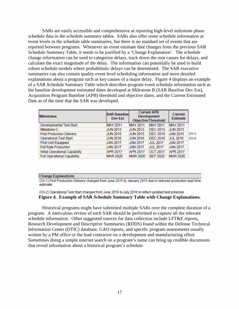
SARs are easily accessible and comprehensive at reporting high-level milestone phase schedule data in the schedule summary tables. SARs also offer some schedule information at event levels in the schedule table summaries, but there is no standard set of events that are reported between programs. Whenever an event estimate date changes from the previous SAR Schedule Summary Table, it needs to be justified by a ‘Change Explanation’. The schedule change information can be used to categorize delays, track down the root causes for delays, and calculate the exact magnitude of the delay. The information can potentially be used to build robust schedule models where probabilistic delays can be determined. The SAR executive summaries can also contain quality event level scheduling information and more detailed explanations about a program such as key causes of a major delay. Figure 4 displays an example of a SAR Schedule Summary Table which describes program event schedule information such as the baseline development estimated dates developed at Milestone B (SAR Baseline Dev Est), Acquisition Program Baseline (APB) threshold and objective dates, and the Current Estimated Date as of the time that the SAR was developed.

Figure 4. Example of SAR Schedule Summary Table with Change Explanations.

Historical programs might have submitted multiple SARs over the complete duration of a program. A meticulous review of each SAR should be performed to capture all the relevant schedule information. Other suggested sources for data collection include LFT&E reports, Research Development and Descriptive Summaries (RDDS) found within the Defense Technical Information Center (DTIC) database, GAO reports, and specific program assessments usually written by a PM office or the lead contractor on a development and manufacturing effort. Sometimes doing a simple internet search on a program’s name can bring up credible documents that reveal information about a historical program’s schedule.

17

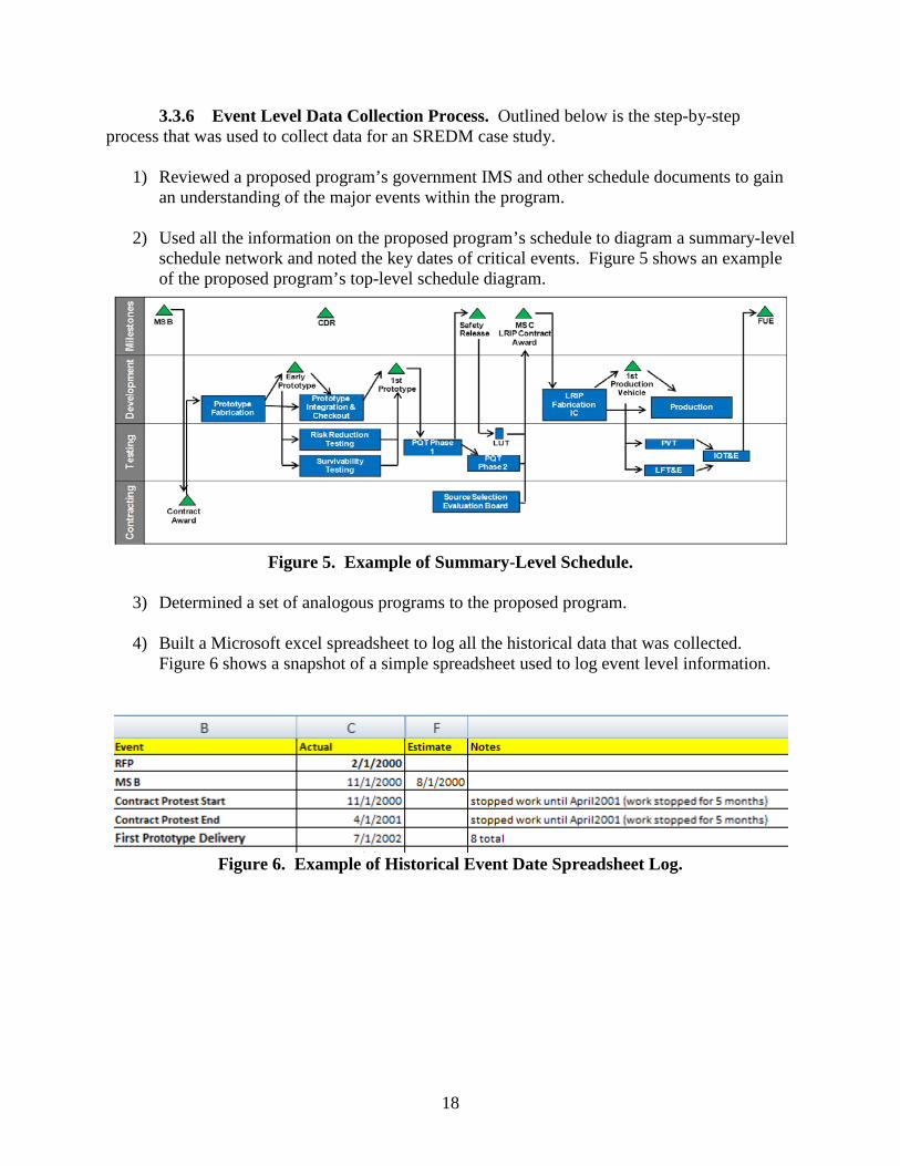
3.3.6 Event Level Data Collection Process. Outlined below is the step-by-step process that was used to collect data for an SREDM case study.

1) Reviewed a proposed program’s government IMS and other schedule documents to gain an understanding of the major events within the program.

2) Used all the information on the proposed program’s schedule to diagram a summary-level schedule network and noted the key dates of critical events. Figure 5 shows an example of the proposed program’s top-level schedule diagram.

Figure 5. Example of Summary-Level Schedule.

3) Determined a set of analogous programs to the proposed program.

4) Built a Microsoft excel spreadsheet to log all the historical data that was collected.

Figure 6 shows a snapshot of a simple spreadsheet used to log event level information.

Figure 6. Example of Historical Event Date Spreadsheet Log.

18

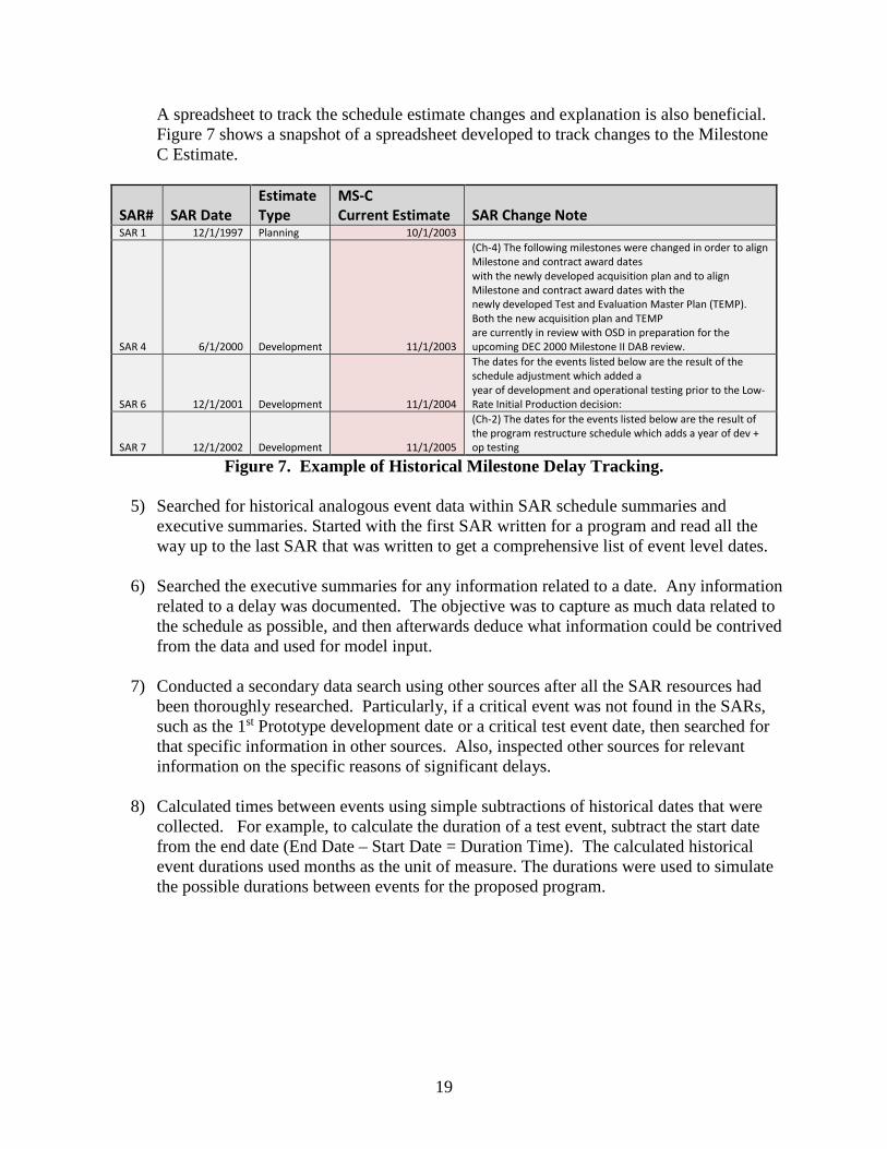
A spreadsheet to track the schedule estimate changes and explanation is also beneficial. Figure 7 shows a snapshot of a spreadsheet developed to track changes to the Milestone C Estimate.

SAR# SAR Date Estimate Type

MS-C Current Estimate SAR Change Note

SAR 1 12/1/1997 Planning 10/1/2003

SAR 4 6/1/2000 Development 11/1/2003

(Ch-4) The following milestones were changed in order to align Milestone and contract award dates with the newly developed acquisition plan and to align Milestone and contract award dates with the newly developed Test and Evaluation Master Plan (TEMP). Both the new acquisition plan and TEMP are currently in review with OSD in preparation for the upcoming DEC 2000 Milestone II DAB review.

SAR 6 12/1/2001 Development 11/1/2004

The dates for the events listed below are the result of the schedule adjustment which added a year of development and operational testing prior to the Low-Rate Initial Production decision:

SAR 7 12/1/2002 Development 11/1/2005

(Ch-2) The dates for the events listed below are the result of the program restructure schedule which adds a year of dev + op testing

Figure 7. Example of Historical Milestone Delay Tracking.

5) Searched for historical analogous event data within SAR schedule summaries and executive summaries. Started with the first SAR written for a program and read all the way up to the last SAR that was written to get a comprehensive list of event level dates.

6) Searched the executive summaries for any information related to a date. Any information related to a delay was documented. The objective was to capture as much data related to the schedule as possible, and then afterwards deduce what information could be contrived from the data and used for model input.

7) Conducted a secondary data search using other sources after all the SAR resources had

been thoroughly researched. Particularly, if a critical event was not found in the SARs, such as the 1st Prototype development date or a critical test event date, then searched for that specific information in other sources. Also, inspected other sources for relevant information on the specific reasons of significant delays.

8) Calculated times between events using simple subtractions of historical dates that were

collected. For example, to calculate the duration of a test event, subtract the start date from the end date (End Date – Start Date = Duration Time). The calculated historical event durations used months as the unit of measure. The durations were used to simulate the possible durations between events for the proposed program.

19

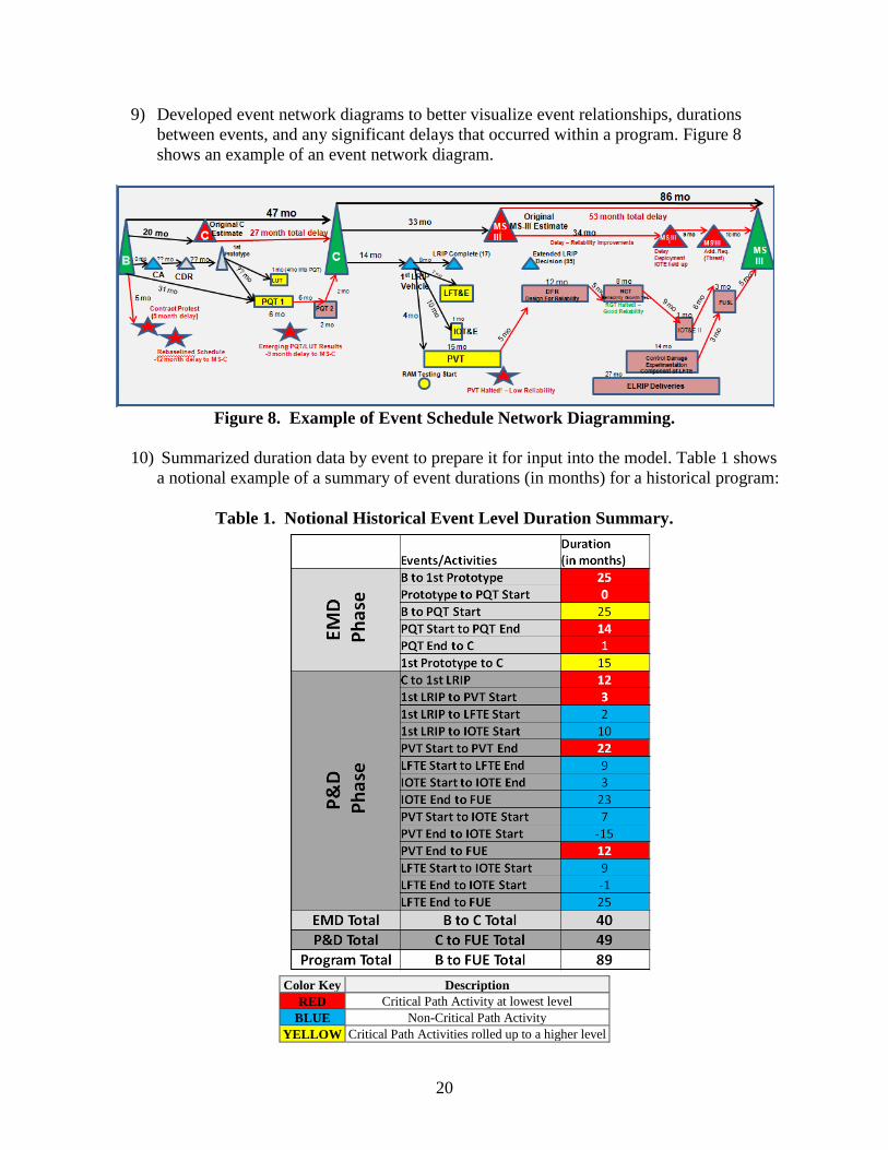
9) Developed event network diagrams to better visualize event relationships, durations between events, and any significant delays that occurred within a program. Figure 8 shows an example of an event network diagram.

Figure 8. Example of Event Schedule Network Diagramming.

10) Summarized duration data by event to prepare it for input into the model. Table 1 shows

a notional example of a summary of event durations (in months) for a historical program:

Table 1. Notional Historical Event Level Duration Summary.

Color Key Description

RED Critical Path Activity at lowest level BLUE Non-Critical Path Activity

YELLOW Critical Path Activities rolled up to a higher level

20

3.4 Case Study Schedule Models.

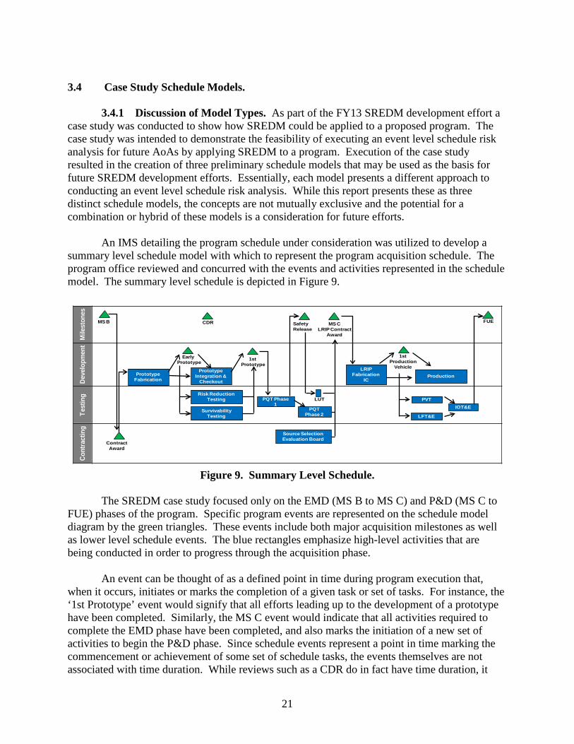
3.4.1 Discussion of Model Types. As part of the FY13 SREDM development effort a case study was conducted to show how SREDM could be applied to a proposed program. The case study was intended to demonstrate the feasibility of executing an event level schedule risk analysis for future AoAs by applying SREDM to a program. Execution of the case study resulted in the creation of three preliminary schedule models that may be used as the basis for future SREDM development efforts. Essentially, each model presents a different approach to conducting an event level schedule risk analysis. While this report presents these as three distinct schedule models, the concepts are not mutually exclusive and the potential for a combination or hybrid of these models is a consideration for future efforts. An IMS detailing the program schedule under consideration was utilized to develop a summary level schedule model with which to represent the program acquisition schedule. The program office reviewed and concurred with the events and activities represented in the schedule model. The summary level schedule is depicted in Figure 9.

Figure 9. Summary Level Schedule.

The SREDM case study focused only on the EMD (MS B to MS C) and P&D (MS C to FUE) phases of the program. Specific program events are represented on the schedule model diagram by the green triangles. These events include both major acquisition milestones as well as lower level schedule events. The blue rectangles emphasize high-level activities that are being conducted in order to progress through the acquisition phase. An event can be thought of as a defined point in time during program execution that, when it occurs, initiates or marks the completion of a given task or set of tasks. For instance, the ‘1st Prototype’ event would signify that all efforts leading up to the development of a prototype have been completed. Similarly, the MS C event would indicate that all activities required to complete the EMD phase have been completed, and also marks the initiation of a new set of activities to begin the P&D phase. Since schedule events represent a point in time marking the commencement or achievement of some set of schedule tasks, the events themselves are not associated with time duration. While reviews such as a CDR do in fact have time duration, it

Mile

ston

esDe

velo

pmen

tTe

stin

gCo

ntra

ctin

g

Contract Award

CDR

1stPrototype

LUT

1stProduction

Vehicle

FUEMS B MS CLRIP Contract

Award

Prototype Fabrication

Early Prototype

Prototype Integration &

Checkout

Risk Reduction Testing

Survivability Testing

PQT Phase 1

Safety Release

PQT Phase 2

Source Selection Evaluation Board

LRIP Fabrication

ICProduction

LFT&E

PVTIOT&E

21

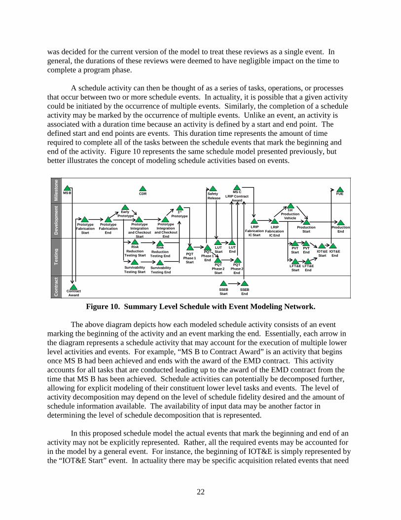
was decided for the current version of the model to treat these reviews as a single event. In general, the durations of these reviews were deemed to have negligible impact on the time to complete a program phase. A schedule activity can then be thought of as a series of tasks, operations, or processes that occur between two or more schedule events. In actuality, it is possible that a given activity could be initiated by the occurrence of multiple events. Similarly, the completion of a schedule activity may be marked by the occurrence of multiple events. Unlike an event, an activity is associated with a duration time because an activity is defined by a start and end point. The defined start and end points are events. This duration time represents the amount of time required to complete all of the tasks between the schedule events that mark the beginning and end of the activity. Figure 10 represents the same schedule model presented previously, but better illustrates the concept of modeling schedule activities based on events.

Figure 10. Summary Level Schedule with Event Modeling Network.

The above diagram depicts how each modeled schedule activity consists of an event marking the beginning of the activity and an event marking the end. Essentially, each arrow in the diagram represents a schedule activity that may account for the execution of multiple lower level activities and events. For example, “MS B to Contract Award” is an activity that begins once MS B had been achieved and ends with the award of the EMD contract. This activity accounts for all tasks that are conducted leading up to the award of the EMD contract from the time that MS B has been achieved. Schedule activities can potentially be decomposed further, allowing for explicit modeling of their constituent lower level tasks and events. The level of activity decomposition may depend on the level of schedule fidelity desired and the amount of schedule information available. The availability of input data may be another factor in determining the level of schedule decomposition that is represented. In this proposed schedule model the actual events that mark the beginning and end of an activity may not be explicitly represented. Rather, all the required events may be accounted for in the model by a general event. For instance, the beginning of IOT&E is simply represented by the “IOT&E Start” event. In actuality there may be specific acquisition related events that need

Mile

ston

eD

evel

opm

ent

Test

ing

Con

trac

t

Contract Award

CDR

1st

Prototype

LUT Start

1stProduction

Vehicle

FUEMS B MS CLRIP Contract

Award

Early Prototype

Safety Release

Prototype Fabrication

Start

Prototype Fabrication

End

Prototype Integration

and Checkout Start

Prototype Integration

and Checkout End

Risk Reduction

Testing Start

Survivability Testing Start

Risk Reduction

Testing End

Survivability Testing End

PQT Phase 1

Start

PQT Phase 1

EndPQT

Phase 2 Start

PQT Phase 2

End

LUT End

SSEB Start

SSEB End

LRIP Fabrication

IC Start

LRIP Fabrication

IC End

PVT Start

PVT End

LFT&E Start

LFT&E End

Production Start

Production End

IOT&E End

IOT&E Start

22

to occur in order to satisfy entry criteria for IOT&E to begin. However, depending on the level of schedule fidelity represented by the model, all of these events may be accounted for by a single event signaling the commencement of IOT&E. The activity duration(s) leading up to the start of IOT&E would assume completion of all these events.

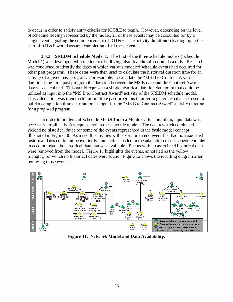
3.4.2 SREDM Schedule Model 1. The first of the three schedule models (Schedule Model 1) was developed with the intent of utilizing historical duration time data only. Research was conducted to identify the dates at which various modeled schedule events had occurred for other past programs. These dates were then used to calculate the historical duration time for an activity of a given past program. For example, to calculate the “MS B to Contract Award” duration time for a past program the duration between the MS B date and the Contract Award date was calculated. This would represent a single historical duration data point that could be utilized as input into the “MS B to Contract Award” activity of the SREDM schedule model. This calculation was then made for multiple past programs in order to generate a data set used to build a completion time distribution as input for the “MS B to Contract Award” activity duration for a proposed program. In order to implement Schedule Model 1 into a Monte Carlo simulation, input data was necessary for all activities represented in the schedule model. The data research conducted yielded no historical dates for some of the events represented in the basic model concept illustrated in Figure 10. As a result, activities with a start or an end event that had no associated historical dates could not be explicitly modeled. This led to the adaptation of the schedule model to accommodate the historical data that was available. Events with no associated historical data were removed from the model. Figure 11 highlights the events, annotated as the yellow triangles, for which no historical dates were found. Figure 12 shows the resulting diagram after removing those events.

Figure 11. Network Model and Data Availability.

23

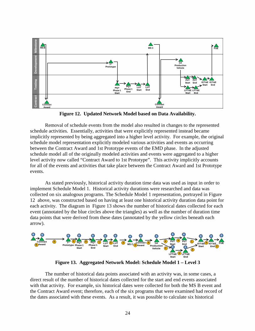
Figure 12. Updated Network Model based on Data Availability.

Removal of schedule events from the model also resulted in changes to the represented schedule activities. Essentially, activities that were explicitly represented instead became implicitly represented by being aggregated into a higher level activity. For example, the original schedule model representation explicitly modeled various activities and events as occurring between the Contract Award and 1st Prototype events of the EMD phase. In the adjusted schedule model all of the originally modeled activities and events were aggregated to a higher level activity now called “Contract Award to 1st Prototype”. This activity implicitly accounts for all of the events and activities that take place between the Contract Award and 1st Prototype events. As stated previously, historical activity duration time data was used as input in order to implement Schedule Model 1. Historical activity durations were researched and data was collected on six analogous programs. The Schedule Model 1 representation, portrayed in Figure 12 above, was constructed based on having at least one historical activity duration data point for each activity. The diagram in Figure 13 shows the number of historical dates collected for each event (annotated by the blue circles above the triangles) as well as the number of duration time data points that were derived from these dates (annotated by the yellow circles beneath each arrow).

Figure 13. Aggregated Network Model: Schedule Model 1 – Level 3

The number of historical data points associated with an activity was, in some cases, a

direct result of the number of historical dates collected for the start and end events associated with that activity. For example, six historical dates were collected for both the MS B event and the Contract Award event; therefore, each of the six programs that were examined had record of the dates associated with these events. As a result, it was possible to calculate six historical

Mile

ston

eD

evel

opm

ent

Test

ing

Con

trac

t

Contract Award

1st

Prototype

LUT Start

1stProduction

Vehicle

FUEMS B MS C

PQT Phase 1

Start

PQT Phase 1

End

LUT End

PVT Start

PVT End

LFT&E Start

LFT&E End

IOT&E End

IOT&E Start

Contract Award

Contract Award

1st

PrototypeLUT Start

1stProduction

Vehicle

FUEMS CPQT

Phase 1 Start

PQT Phase 1

End

LUT End

PVT Start

PVT End

LFT&E Start

LFT&E End

IOT&E End

IOT&E Start

6 6 5 5 4 4 44

4

4 3

Contract Award

45 4 4

4

4

65 5 5 1 4 3

44

3

4 4

4

1

2

43

24

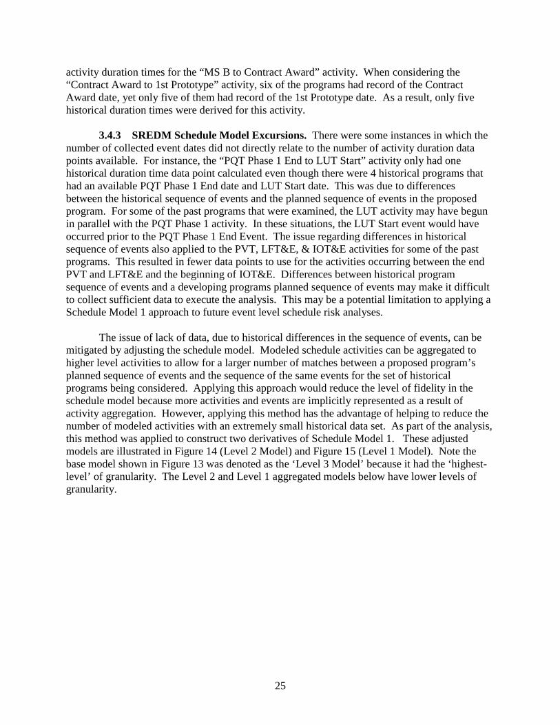
activity duration times for the “MS B to Contract Award” activity. When considering the “Contract Award to 1st Prototype” activity, six of the programs had record of the Contract Award date, yet only five of them had record of the 1st Prototype date. As a result, only five historical duration times were derived for this activity.

3.4.3 SREDM Schedule Model Excursions. There were some instances in which the number of collected event dates did not directly relate to the number of activity duration data points available. For instance, the “PQT Phase 1 End to LUT Start” activity only had one historical duration time data point calculated even though there were 4 historical programs that had an available PQT Phase 1 End date and LUT Start date. This was due to differences between the historical sequence of events and the planned sequence of events in the proposed program. For some of the past programs that were examined, the LUT activity may have begun in parallel with the PQT Phase 1 activity. In these situations, the LUT Start event would have occurred prior to the PQT Phase 1 End Event. The issue regarding differences in historical sequence of events also applied to the PVT, LFT&E, & IOT&E activities for some of the past programs. This resulted in fewer data points to use for the activities occurring between the end PVT and LFT&E and the beginning of IOT&E. Differences between historical program sequence of events and a developing programs planned sequence of events may make it difficult to collect sufficient data to execute the analysis. This may be a potential limitation to applying a Schedule Model 1 approach to future event level schedule risk analyses. The issue of lack of data, due to historical differences in the sequence of events, can be mitigated by adjusting the schedule model. Modeled schedule activities can be aggregated to higher level activities to allow for a larger number of matches between a proposed program’s planned sequence of events and the sequence of the same events for the set of historical programs being considered. Applying this approach would reduce the level of fidelity in the schedule model because more activities and events are implicitly represented as a result of activity aggregation. However, applying this method has the advantage of helping to reduce the number of modeled activities with an extremely small historical data set. As part of the analysis, this method was applied to construct two derivatives of Schedule Model 1. These adjusted models are illustrated in Figure 14 (Level 2 Model) and Figure 15 (Level 1 Model). Note the base model shown in Figure 13 was denoted as the ‘Level 3 Model’ because it had the ‘highest-level’ of granularity. The Level 2 and Level 1 aggregated models below have lower levels of granularity.

25

Figure 14. Aggregated Network Model: Schedule Model 1 – Level 2.

Figure 15. Aggregated Network Model: Schedule Model 1 – Level 1

In Figure 14, the PQT Phase 1 Start and PQT Phase 1 End events were removed. This resulted in the removal of the “1st Prototype to PQT Phase 1 Start”, “PQT Phase 1 Start to PQT Phase 1 End”, and “PQT Phase 1 End to LUT Start” activities, which were aggregated to derive the “1st Prototype to LUT Start” activity. In this case, instead of having two activities with six data points and one activity with one data point, the model instead represented an aggregated activity with three data points. When activities were aggregated further, as in Figure 15, the result was a new activity, “1st Prototype to MS C”, which had six data points, but with more activities and events implicitly modeled. Similar changes were made to other activities and events within the schedule model. Notice that the schedule model derivative in Figure 15 represents significantly fewer activities, five in total, than the original schedule 1 model in Figure 13. Various other derivative models could have been explored as well in order to determine an optimal model which would maximize the number of explicitly modeled activities, while minimizing the number of activities with only one historical data point. However, due to time constraints, the SREDM analysis that was conducted using the Schedule Model 1 approach only considered the three models presented in this section. Another potential method to mitigate the issue of historical sequence of events that was not considered in the analysis is to assume a time duration of zero for those past programs in which the sequence of event do not align with the planned sequence of the new program. For example, it was mentioned previously that a given past program may have had a LUT Start event that occurred prior to the PQT Phase 1 End event. In this situation a historical duration time for the “PQT Phase 1 End and LUT Start” activity could not be calculated from this program. Since for this specific program, the LUT began during the PQT Phase 1 activity, an assumption could be made that had this program planned to conduct the LUT after completion of the PQT Phase 1 it could have done so immediately. This would then imply a duration time of zero from the PQT Phase 1 End event to the LUT Start event. This may be a reasonable assumption to make; however, there may have also been other tasks that had to be completed prior to the LUT Start which were conducted in parallel with execution of the PQT Phase 1 activity. If the plan had been to conduct the LUT following completion of the PQT Phase 1 activity it’s possible that these other tasks would not have been started until the completion of PQT Phase 1. If this were the case, then an assumption of zero duration between PQT Phase 1 End and LUT start may not be valid.

Contract Award

1st

PrototypeLUT Start

1stProduction

Vehicle

FUEMS B

MS C

PQT Phase 1

Start

PQT Phase 1

End

LUT End PVT

StartPVT End

LFT&E Start

LFT&E End

IOT&E End

IOT&E Start

6 6 5 4 4 4 4 3

Contract Award

4 4

65 3 4 3 4 4

43

Contract Award

1st

Prototype

LUT Start

1stProduction

Vehicle

FUEMS BMS C

PQT Phase 1

Start

PQT Phase 1

End

LUT End

PVT Start

PVT End

LFT&E Start

LFT&E End

IOT&E End

IOT&E Start

6 6 5 4 4 3

Contract Award

65 5 4 3

26

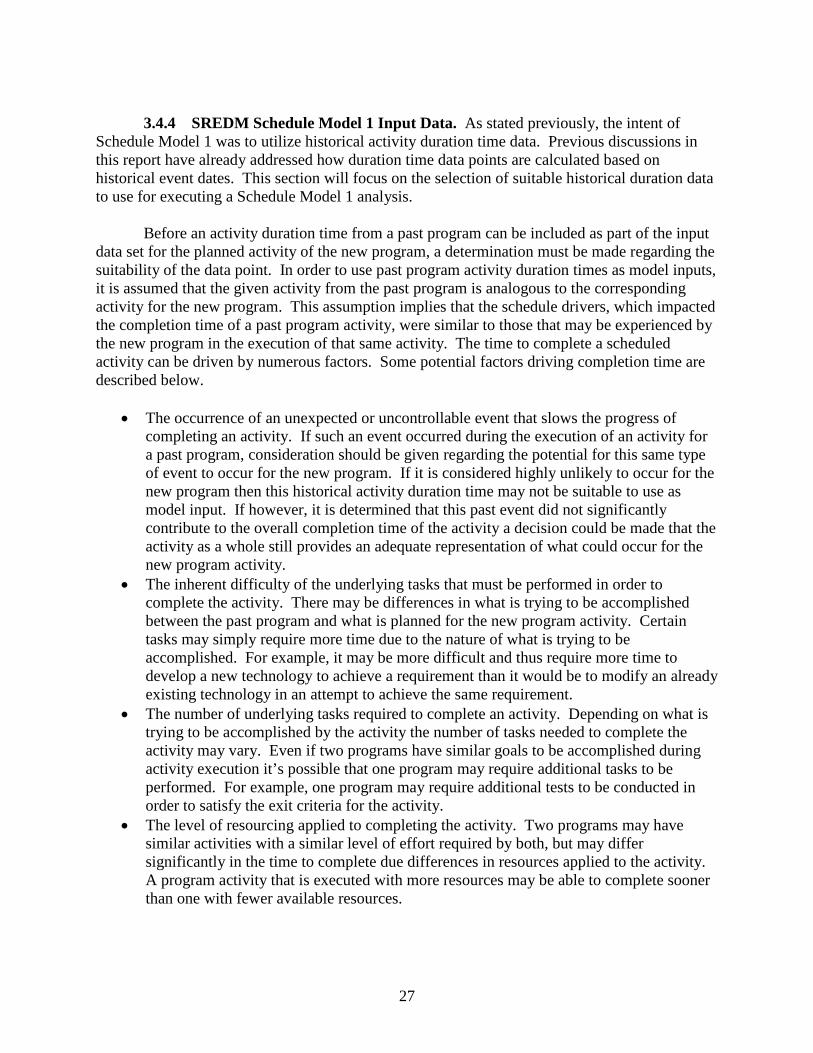
3.4.4 SREDM Schedule Model 1 Input Data. As stated previously, the intent of

Schedule Model 1 was to utilize historical activity duration time data. Previous discussions in this report have already addressed how duration time data points are calculated based on historical event dates. This section will focus on the selection of suitable historical duration data to use for executing a Schedule Model 1 analysis. Before an activity duration time from a past program can be included as part of the input data set for the planned activity of the new program, a determination must be made regarding the suitability of the data point. In order to use past program activity duration times as model inputs, it is assumed that the given activity from the past program is analogous to the corresponding activity for the new program. This assumption implies that the schedule drivers, which impacted the completion time of a past program activity, were similar to those that may be experienced by the new program in the execution of that same activity. The time to complete a scheduled activity can be driven by numerous factors. Some potential factors driving completion time are described below.

• The occurrence of an unexpected or uncontrollable event that slows the progress of completing an activity. If such an event occurred during the execution of an activity for a past program, consideration should be given regarding the potential for this same type of event to occur for the new program. If it is considered highly unlikely to occur for the new program then this historical activity duration time may not be suitable to use as model input. If however, it is determined that this past event did not significantly contribute to the overall completion time of the activity a decision could be made that the activity as a whole still provides an adequate representation of what could occur for the new program activity.

• The inherent difficulty of the underlying tasks that must be performed in order to complete the activity. There may be differences in what is trying to be accomplished between the past program and what is planned for the new program activity. Certain tasks may simply require more time due to the nature of what is trying to be accomplished. For example, it may be more difficult and thus require more time to develop a new technology to achieve a requirement than it would be to modify an already existing technology in an attempt to achieve the same requirement.

• The number of underlying tasks required to complete an activity. Depending on what is trying to be accomplished by the activity the number of tasks needed to complete the activity may vary. Even if two programs have similar goals to be accomplished during activity execution it’s possible that one program may require additional tasks to be performed. For example, one program may require additional tests to be conducted in order to satisfy the exit criteria for the activity.

• The level of resourcing applied to completing the activity. Two programs may have similar activities with a similar level of effort required by both, but may differ significantly in the time to complete due differences in resources applied to the activity. A program activity that is executed with more resources may be able to complete sooner than one with fewer available resources.

27

It is unlikely that an activity from a past program will be identical in terms of schedule drivers to the corresponding planned activity for a new program. The goal in selecting an appropriate past program analogy for the activity is to identify activities that are similar. The degree to which the new program activity is similar to the past program activity in terms of the expected schedule drivers will determine the strength of the analogous assumption. Stronger analogies build confidence that the input data set, used to generate an activity completion time distribution, adequately represents the variability regarding the time to complete the activity. The process of aggregating activities within the schedule model could potentially lead to weaker analogies. Recall that the aggregation of multiple lower level events and activities into a single higher level activity resulted in the implicit modeling of those lower level activities and events. As a result, a time duration input to this higher level activity would account for the time to complete all of the implied underlying activities. In determining if the activity from a past program is analogous to this higher level activity of the new program, a larger set of potential schedule drivers would have to be compared with the past program. A past program that may have been very similar to the new program in one of the underlying activities may not be as similar to the other activities within the higher level activity. So, while this given program may have provided a strong analogy for one activity, it may not be as similar when applied to the higher level activity. This concept highlights one of the strengths of conducting an event level analysis. By decomposing schedule activities into smaller activities it may become easier to find a historical activity that is similar in terms of schedule drivers. The analogous datasets used to generate completion time distributions for the SREDM Schedule Model 1 analysis were determined based on input from a panel of SMEs. The selection process conducted by the SMEs was focused on identifying past programs whose program phases as a whole would be considered analogous to the corresponding phases of the new program. The SREDM analysis assumed that the individual underlying activities within the phases of these past programs would also be analogous to the corresponding underlying activities for the new program.

3.4.5 SREDM Schedule Model 1 Monte Carlo Simulation. The objective of the analysis was to construct a Monte Carlo simulation that utilized the structure and logic represented by the schedule model along with the associated input data for each of the modeled activities. Development of this simulation provided the capability to simulate execution of the program in order to determine a completion time outcome for each of the program phases. This was replicated multiple times in order to generate a set of potential completion time outcomes for each of the schedule phases. Schedule Model 1 along with the two presented derivative models were each implemented into a Monte Carlo simulation.

3.4.6 SREDM Schedule Model 1 Monte Carlo Input Data. A given schedule activity was represented in the simulation by its associated completion time distribution. The Monte Carlo simulation utilized these completion time distributions to draw random values in regards to the completion time for each of the modeled activities. Each time the simulation was replicated a completion time value was drawn at random for each activity. This provided the source of randomness which ultimately drove the variability in the resulting phase completion time dataset.

28

The historical time duration datasets, derived for the set of past analogous program activities, were used to generate completion time distributions for each of the modeled activities. In this analysis, only empirical distributions were used. Thus, a given distribution was represented by only the actual observed values derived from each of the past programs that were considered. The observed set of data could be fit to a theoretical distribution; however, it may not always be possible to fit the data to a theoretical distribution, in which case the empirical set of observed data is used as the representative distribution. Recall that for the base Schedule Model 1 representation there were a couple of activities which only had a single duration time input. In the implementation of this model, only the single value was utilized as an input. In this case, the same value was used for every replication of the simulation. This effectively resulted in a deterministic modeling of that specific activity.

3.4.7 SREDM Schedule Model 1 Monte Carlo Logic. The model logic defined how, for a single simulation replication, a set of schedule activities and randomly generated completion time values associated with each would be combined to generate a single phase completion time outcome. The logic that defines the relationship between each modeled event and activity was coded into the simulation software. Schedule Model 1 considered two types of schedule relationships regarding activity execution: sequential and parallel. Two activities were considered to have a sequential relationship if the event that marked the end of one activity also signaled the beginning of the next activity. This implies that all tasks accounted for by the previous activity must be completed in order to begin the next activity. The length of time required to achieve the final event in the series was calculated by summing the two random completion time draws from both of the activities. Expanding upon this further, the total completion time of a series of sequential activities was calculated by simply summing all of the completion times for each individual activity. The Schedule Model 1 approach of representing sequential activity execution assumed that there was no correlation between the completion times of each activity. As a result, the model was implemented such that the time required to complete the first activity in a sequential pair had no impact on the time required to complete the second activity. Therefore, random completion times for two sequential activities were drawn independently. Similar to the representation of sequential activity execution, the Schedule Model 1 representation of parallel activity execution assumed that there was no relationship between the completion times of activities. As a result, random completion times for activities executed in parallel were drawn independently. This assumption implies that there were no interdependencies amongst the underlying tasks being performed between any set of parallel activities. Further analysis on historical data should be conducted to investigate the validity of the assumption that completion times for the sequential and parallel activities represented by Schedule Model 1 are independent. A set of past programs could be examined to determine if the completion times of certain activities, executed either in sequence or in parallel, have historically exhibited any type of relationship. This may uncover instances in which a longer

29

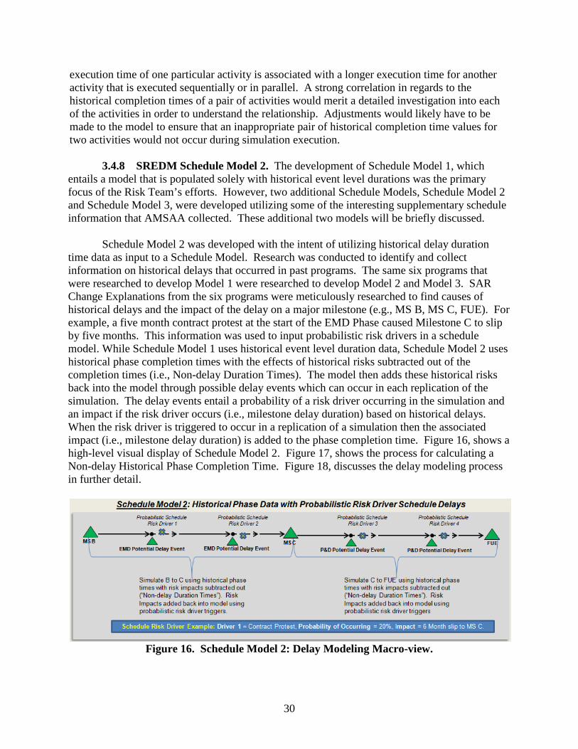
execution time of one particular activity is associated with a longer execution time for another activity that is executed sequentially or in parallel. A strong correlation in regards to the historical completion times of a pair of activities would merit a detailed investigation into each of the activities in order to understand the relationship. Adjustments would likely have to be made to the model to ensure that an inappropriate pair of historical completion time values for two activities would not occur during simulation execution.

3.4.8 SREDM Schedule Model 2. The development of Schedule Model 1, which entails a model that is populated solely with historical event level durations was the primary focus of the Risk Team’s efforts. However, two additional Schedule Models, Schedule Model 2 and Schedule Model 3, were developed utilizing some of the interesting supplementary schedule information that AMSAA collected. These additional two models will be briefly discussed. Schedule Model 2 was developed with the intent of utilizing historical delay duration time data as input to a Schedule Model. Research was conducted to identify and collect information on historical delays that occurred in past programs. The same six programs that were researched to develop Model 1 were researched to develop Model 2 and Model 3. SAR Change Explanations from the six programs were meticulously researched to find causes of historical delays and the impact of the delay on a major milestone (e.g., MS B, MS C, FUE). For example, a five month contract protest at the start of the EMD Phase caused Milestone C to slip by five months. This information was used to input probabilistic risk drivers in a schedule model. While Schedule Model 1 uses historical event level duration data, Schedule Model 2 uses historical phase completion times with the effects of historical risks subtracted out of the completion times (i.e., Non-delay Duration Times). The model then adds these historical risks back into the model through possible delay events which can occur in each replication of the simulation. The delay events entail a probability of a risk driver occurring in the simulation and an impact if the risk driver occurs (i.e., milestone delay duration) based on historical delays. When the risk driver is triggered to occur in a replication of a simulation then the associated impact (i.e., milestone delay duration) is added to the phase completion time. Figure 16, shows a high-level visual display of Schedule Model 2. Figure 17, shows the process for calculating a Non-delay Historical Phase Completion Time. Figure 18, discusses the delay modeling process in further detail.

Figure 16. Schedule Model 2: Delay Modeling Macro-view.

30

Figure 17. Schedule Model 2: Calculating Non-delay Phase Completion Durations.

Figure 18. Schedule Model 2: Delay Modeling Micro-view.

Determining an accurate probability for the occurrence of the delay event in the proposed program was an aspect of the model that did not undergo severe scrutiny. Notional probabilities were used in the case study to exercise the model. However, various excursions and sensitivities were simulated to see the affect of changing the delay event probabilities. For example, attaching a zero percent probability to all delay events was one of the excursions that was modeled to develop a schedule distribution based off the scenario that no significant risk drivers will occur in the program. As historical delay data is researched and data based then delay probabilities could potentially be based off historical frequencies. For example, if historically contract protests occurred in 10 of 100 past programs, then the contract protest risk driver would acquire a 10% chance of being triggered in a model.

3.4.9 SREDM Schedule Model 3. Schedule Model 3 was developed with the intent of integrating AMSAA’s technical risk methodology and schedule risk assessment methodology in order to support technology trades. Particularly, model 3 was an attempt to utilize the Key Technology (KT) development time distributions that AMSAA collects from SMEs at Risk Workshops in an event driven model. The data used to formulate KT time distributions was briefly discussed in section 3.3.4. The data pertains to estimated times for a KT to achieve certain TRL, IRL, and MRL levels by key milestone dates. The resulting KT development duration data was used to simulate the EMD phase within Schedule Model 3. Course of Action (COA) input from the PM is also utilized to assist with modeling KT development within the EMD Phase. For example, in a given scenario that a KT has not matured as planned by a Milestone date then the PM might say the KT will be accepted as-is instead of delaying the schedule to allow the KT to achieve its full maturity level. The P&D Phase in Schedule Model 3 is simulated exactly like the Schedule 1 Model, relying on solely historical event duration data.

31

Figure 19 shows a high-level visual display of SREDM Schedule Model 3. Figure 20 discusses the use of KT data within the model in further detail.

Figure 19. Schedule Model 3: KT Development Modeling – Macro-view.

Figure 20. Schedule Model 3: KT Development Modeling – Micro-view.

32

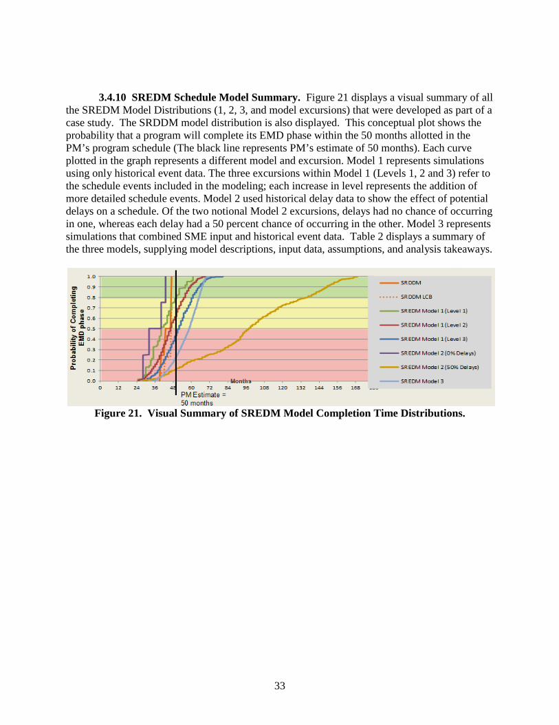
3.4.10 SREDM Schedule Model Summary. Figure 21 displays a visual summary of all the SREDM Model Distributions (1, 2, 3, and model excursions) that were developed as part of a case study. The SRDDM model distribution is also displayed. This conceptual plot shows the probability that a program will complete its EMD phase within the 50 months allotted in the PM’s program schedule (The black line represents PM’s estimate of 50 months). Each curve plotted in the graph represents a different model and excursion. Model 1 represents simulations using only historical event data. The three excursions within Model 1 (Levels 1, 2 and 3) refer to the schedule events included in the modeling; each increase in level represents the addition of more detailed schedule events. Model 2 used historical delay data to show the effect of potential delays on a schedule. Of the two notional Model 2 excursions, delays had no chance of occurring in one, whereas each delay had a 50 percent chance of occurring in the other. Model 3 represents simulations that combined SME input and historical event data. Table 2 displays a summary of the three models, supplying model descriptions, input data, assumptions, and analysis takeaways.

Figure 21. Visual Summary of SREDM Model Completion Time Distributions.

33

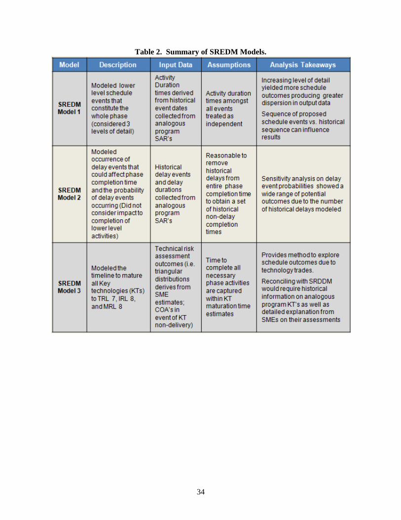
Table 2. Summary of SREDM Models.

34

4. VERIFICATION AND VALIDATION (V&V) PLAN Part of the FY13 effort was to develop a plan for the verification and validation of the risk assessment models. An initial verification and validation plan was created for SRDDM and SREDM along with a conceptualization for an output validation hypothesis testing procedure to evaluate the accuracy of the distributions of outcomes for the various methods. The verification activities will determine that all procedures are implemented correctly. The validation activities will determine the degree in which the mathematical model accurately represents the real world from the perspective of the models intended use (assess probability of phase completion) [Reference 9]. The first step for the validation is to assure all the model parts or pieces reflect reality. This is mostly a face validation conducted with suitable SMEs. Some of these parts include:

• Analogous data (phase, event, etc.) • SME based (events) and the elicitation methods used • Model schedule network logic and correlation between events • Other important information.

The next step for validation is to conduct an output analysis on any pieces (event or entire phase) where completion data can be collected and characteristics can be obtained at the beginning of the phase or event. A single decision or process cannot be validated¸ only repetitive processes. A bad outcome does not imply a bad decision [Reference 10]. Some repetitive processes are more defined than others. For example, approving 10,000 customers for a credit score based on a credit scoring process and collecting each individual outcome (good or bad customer) is very defined repetitive process. Conducting schedule risk assessments for 15 different AoA alternatives using the SRDDM method is considered to be a repetitive process. Performing the output validation is different for the credit card and AoA alternative processes. The credit card approach can bin the scores and observe the results (i.e., a gains chart) since there are thousands of outcomes, whereas the AoA alternative approach requires a hypothesis test approach, since the sample sizes are small.

35

5. CONCLUSION To build upon the initial success of SRDDM, AMSAA endeavored to find historical duration time data for lower level events within each acquisition phase and to utilize this data in corresponding statistical schedule risk assessment models. AMSAA successfully collected event level duration data, historical delay data to develop a set of preliminary SREDM models. A V&V plan was also developed that will be implemented to evaluate how well the schedule models realistically assess schedule distributions.

An event level risk assessment approach promotes greater flexibility in the use of historical data within the model, and offers the capability to model additional schedule complexities. For instance, a PM may be interested in conducting a trade-off analysis to compare the schedule impact of pursuing various technology solutions. With an event level approach, the PM could look at past examples of technology development and the technology’s associated schedule impact at the event level rather than at the phase level. Event level historical durations of similar programs may provide greater confidence in the PM’s outlined schedule if the PM’s estimates align with historical data or help to illuminate particular risky parts of the schedule if the PM’s estimates do not coincide with historical examples. The PM can also better understand the historical risks and consequences of pursuing a risky technology, and they might want to avoid these historical consequences by pursuing less risky technologies or mitigate a risk through applying mitigation strategies to a given technology or event.

The development of SREDM provides acquisition schedule risk insight gained from analyzing historical programs at the event level, the potential implications of the event data to enhance risk modeling, and the lessons learned from the process of developing an event level schedule risk modeling approach. The SREDM research lays strong foundation for future schedule risk methodology research.

5.1 Path Forward. AMSAA will seek to continuously enhance the risk assessment approaches at both the event level and phase level to ensure that the significant ramifications of all critical sources of schedule risk are being assessed in a realistic, unbiased, and rational manner. AMSAA also plans to continuously search for other methods to enhance schedule risk assessment approaches by seeking out new or enhanced tools, data, process, and knowledge. Of particular interest is researching and developing tools to select and adjust analogous program schedule data based on historical program schedule driver data (i.e., program characteristic data that is shown to have a statistically significant affect on schedule completion time). Historical databases of acquisition data will be established to help build these tools and the databases will be a tool to assist with carrying out risk assessments and further research. Risk assessment processes will be continuously assessed for gains in efficiency and effectiveness. In terms of knowledge, AMSAA seeks to leverage the expertise of other acquisition organizations to help socialize and develop risk assessment models. With strong collaboration from the acquisition community and new and improved tools, processes, data and access to data, the AMSAA will proceed toward its goal of providing the best possible product—an independent, honest and accurate schedule risk assessment.

36

REFERENCES 1.

Office of the Under Secretary of Defense, Acquisition, Technology and Logistics, Performance of the Defense Acquisition System Report, 2013 Annual Report

2. United States Government Accountability Office, Report to Congressional Committees, Defense Management, “Guidance and Progress Measures Are Needed to Realize Benefits from Changes in DOD’s Joint Requirements Process”, GAO-12-339, February 2012

3.

Department of Defense, Risk Management Guide for DoD Acquisitions (Sixth Edition), August 2006

4. Flyvbjerg, “Curbing Optimism Bias and Strategic Misrepresentation in Planning: Reference Class Forecasting in Practice”, European Planning Studies Vol. 16, No. 1, January 2008, pp. 3-21

5.

Nierwinski, J., “Schedule Risk Data Decision Methodology (SRDDM)”, AMSAA TR-2012-65, September 2012

6. Yoon & Hwang, “Multiple Attribute Decision Making”, SAGE, 1995 7. Vose, “Risk Analysis: A Quantitative Guide (Third Edition)”, John Wiley & Sons, 2008 8. Naval Air Systems Command, NAVAIR Risk Assessment Handbook, 2002 9. Law, A.M., “Simulation Modeling and Analysis (Fourth Edition)”, McGraw Hill,

Boston, 2007 10. Clemen & Reilly, “Making Hard Decisions with Decision Tools”, South Western, 2001

37

THIS PAGE INTENTIONALLY LEFT BLANK.

38

APPENDIX A – DISTRIBUTION LIST

A-1

THIS PAGE INTENTIONALLY LEFT BLANK.

A-2

DISTRIBUTION LIST Organization US Army Materiel Systems Analysis Activity AMXAA-GL/Reports Processing 392 Hopkins Rd. Aberdeen Proving Ground, MD 21005-5071 US Army TRADOC Analysis Center ATRC-PR/Susan Matus 255 Sedgwick Avenue Fort Leavenworth, KS 66027-2345 susan.g.matus.civ@mail.mil US Army TRAC- White Sands Missile Range ATRC-W/Dr. Lambert Bldg 1400 Martin Luther King Drive White Sands Missile Range, NM 88002-5502 garrett.r.lambert.civ@mail.mil Defense Technical Information Center ATTN: DTIC-O 8725 John J. Kingman Rd Fort Belvoir, VA 22060-6218 jackie.l.rike.civ@dtic.mil Office of the Deputy Chief of Staff, G-3/5/7 DAMO-CIA/COL George Seaward DAMO-CIA/Mr. Michael Moore 4000 Army Pentagon (Room 2E382) Washington, DC 20310-0400 george.h.seaward.civ@mail.mil michael.j.moore.civ@mail.mil

A-3

DISTRIBUTION LIST (cont) Organization Army Capabilities Integration Center (ARCIC) COL Thomas E Dillingham 950 Jefferson Avenue Ft. Eustis, VA 23604-5761 thomas.e.dillingham4.mil@mail.mil Center for Army Analysis (CAA) Dr. Forrest Crain 6001 Goethais Road Ft. Belvoir, VA 22060-5230 william.f.crain.civ@mail.mil

A-4

THIS PAGE INTENTIONALLY LEFT BLANK.

A-5