Technical Report Documentation Page 1. Report … http:// 16. Abstract Prestressed concrete I-beams are used extensively as the primary superstructure components in Texas highway bridges

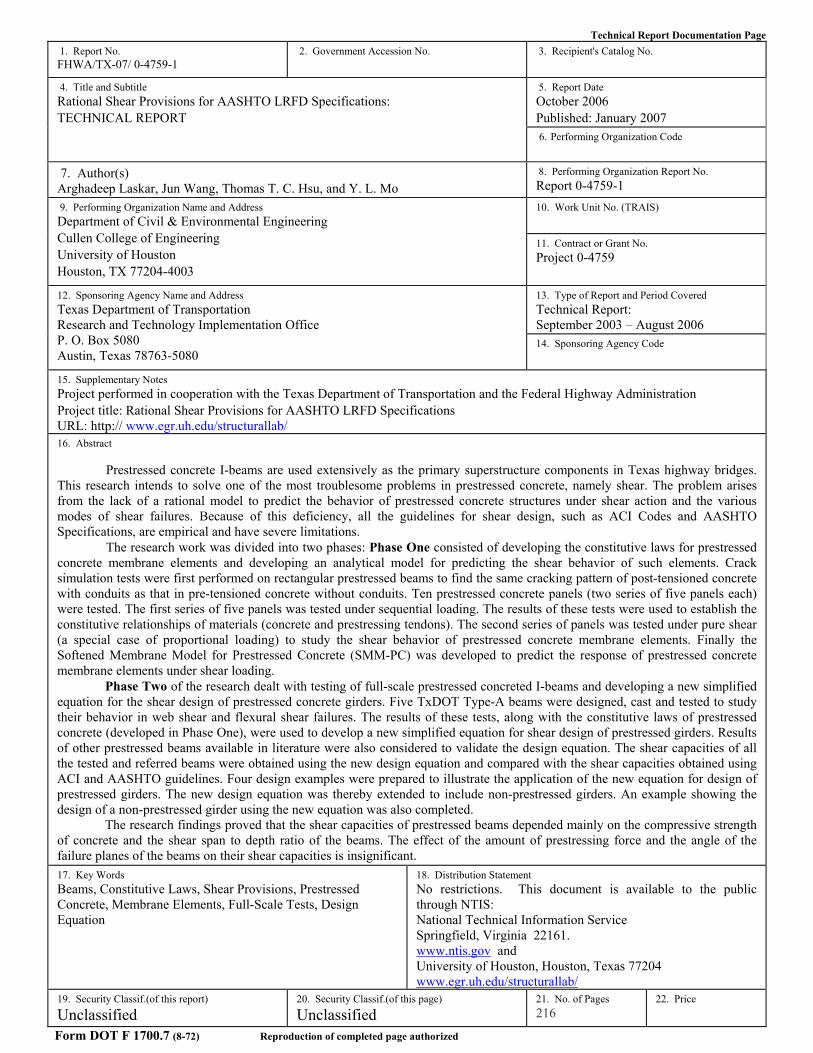
Technical Report Documentation Page 1. Report No. FHWA/TX-07/ 0-4759-1

2. Government Accession No.

3. Recipient's Catalog No.

5. Report Date October 2006 Published: January 2007

4. Title and Subtitle Rational Shear Provisions for AASHTO LRFD Specifications: TECHNICAL REPORT

6. Performing Organization Code

7. Author(s) Arghadeep Laskar, Jun Wang, Thomas T. C. Hsu, and Y. L. Mo

8. Performing Organization Report No. Report 0-4759-1 10. Work Unit No. (TRAIS)

9. Performing Organization Name and Address Department of Civil & Environmental Engineering Cullen College of Engineering University of Houston Houston, TX 77204-4003

11. Contract or Grant No. Project 0-4759

13. Type of Report and Period Covered Technical Report: September 2003 – August 2006

12. Sponsoring Agency Name and Address Texas Department of Transportation Research and Technology Implementation Office P. O. Box 5080 Austin, Texas 78763-5080

14. Sponsoring Agency Code

15. Supplementary Notes Project performed in cooperation with the Texas Department of Transportation and the Federal Highway Administration Project title: Rational Shear Provisions for AASHTO LRFD Specifications URL: http:// www.egr.uh.edu/structurallab/ 16. Abstract

Prestressed concrete I-beams are used extensively as the primary superstructure components in Texas highway bridges. This research intends to solve one of the most troublesome problems in prestressed concrete, namely shear. The problem arises from the lack of a rational model to predict the behavior of prestressed concrete structures under shear action and the various modes of shear failures. Because of this deficiency, all the guidelines for shear design, such as ACI Codes and AASHTO Specifications, are empirical and have severe limitations.

The research work was divided into two phases: Phase One consisted of developing the constitutive laws for prestressed concrete membrane elements and developing an analytical model for predicting the shear behavior of such elements. Crack simulation tests were first performed on rectangular prestressed beams to find the same cracking pattern of post-tensioned concrete with conduits as that in pre-tensioned concrete without conduits. Ten prestressed concrete panels (two series of five panels each) were tested. The first series of five panels was tested under sequential loading. The results of these tests were used to establish the constitutive relationships of materials (concrete and prestressing tendons). The second series of panels was tested under pure shear (a special case of proportional loading) to study the shear behavior of prestressed concrete membrane elements. Finally the Softened Membrane Model for Prestressed Concrete (SMM-PC) was developed to predict the response of prestressed concrete membrane elements under shear loading.

Phase Two of the research dealt with testing of full-scale prestressed concreted I-beams and developing a new simplified equation for the shear design of prestressed concrete girders. Five TxDOT Type-A beams were designed, cast and tested to study their behavior in web shear and flexural shear failures. The results of these tests, along with the constitutive laws of prestressed concrete (developed in Phase One), were used to develop a new simplified equation for shear design of prestressed girders. Results of other prestressed beams available in literature were also considered to validate the design equation. The shear capacities of all the tested and referred beams were obtained using the new design equation and compared with the shear capacities obtained using ACI and AASHTO guidelines. Four design examples were prepared to illustrate the application of the new equation for design of prestressed girders. The new design equation was thereby extended to include non-prestressed girders. An example showing the design of a non-prestressed girder using the new equation was also completed.

The research findings proved that the shear capacities of prestressed beams depended mainly on the compressive strength of concrete and the shear span to depth ratio of the beams. The effect of the amount of prestressing force and the angle of the failure planes of the beams on their shear capacities is insignificant. 17. Key Words Beams, Constitutive Laws, Shear Provisions, Prestressed Concrete, Membrane Elements, Full-Scale Tests, Design Equation

18. Distribution Statement No restrictions. This document is available to the public through NTIS: National Technical Information Service Springfield, Virginia 22161. www.ntis.gov and University of Houston, Houston, Texas 77204 www.egr.uh.edu/structurallab/

19. Security Classif.(of this report)

Unclassified

20. Security Classif.(of this page)

Unclassified

21. No. of Pages 216

22. Price

Form DOT F 1700.7 (8-72) Reproduction of completed page authorized

www.ntis.gov

www.egr.uh.edu/structurallab/

www.egr.uh.edu/structurallab/

Rational Shear Provisions for AASHTO LRFD

Specifications: Technical Report

by

Arghadeep Laskar Research Assistant

Jun Wang

Research Assistant

Thomas T. C. Hsu Moores Professor

and

Y. L. Mo Professor

Report 0-4759-1 Project 0-4759

Project Title: Rational Shear Provisions for AASHTO LRFD Specifications

Performed in cooperation with the Texas Department of Transportation

and the Federal Highway Administration

October 2006 Published: January 2007

Department of Civil and Environmental Engineering

University of Houston

Houston, Texas

iv

v

DISCLAIMER This research was performed in cooperation with the Texas Department of Transportation and the U.S. Department of Transportation, Federal Highway Administration. The contents of this report reflect the views of the authors, who are responsible for the facts and accuracy of the data presented herein. The contents do not necessarily reflect the official view or policies of the FHWA or TxDOT. This report does not constitute a standard, specification, or regulation, nor is it intended for construction, bidding, or permit purposes. Trade names were used solely for information and not product endorsement.

vii

ACKNOWLEDGEMENTS This research, Project 0-4759, was conducted in cooperation with the Texas Department of Transportation and the U.S. Department of Transportation, Federal Highway Administration. The project monitoring committee consisted of J. C. Liu (Program Coordinator), Jon Holt (Project Director), Tim Bradberry (Project Advisor), Amy Eskridge (Project Advisor), Mark Holt (Project Advisor), John Vogel (Project Advisor), and Tom Yarbrough (Project Advisor).

The researchers would like to thank the Texas Concrete Company, Victoria, Texas, for continued co-operation during this project. The researchers are grateful to Chaparrel Steel Co. of Midlothian, Texas, for supplying the steel bars for this research.

viii

ix

TABLE OF CONTENTS

Page CHAPTER 1 Introduction ....................................................................................................1 1.1 Overview of Research....................................................................................................1 1.2 Objectives of Research ..................................................................................................4 1.3 Outline of Report ...........................................................................................................4

PART I: PRESTRESSED CONCRETE ELEMENTS

CHAPTER 2 Backgrounds on Shear Theories of Reinforced and Prestressed Concrete Panels ............................................................................................................9 2.1 Introduction....................................................................................................................9 2.2 Shear Theories of Reinforced Concrete in Literature ....................................................9 2.3 Previous Studies by Research Group at UH ................................................................12 2.3.1 Rotating-Angle Softened Truss Model (RA-STM) .........................................15 2.3.2 Fixed-Angle Softened Truss Model (FA-STM) ..............................................17 2.3.3 Softened Membrane Model (SMM).................................................................20 2.4 Literature Survey on Shear Behavior of Prestressed Concrete Panels ........................27 CHAPTER 3 Crack Simulation Tests................................................................................29 3.1 General Description .....................................................................................................29 3.2 Test Program................................................................................................................31 3.3 Test Specimens ............................................................................................................33 3.3.1 Fabrication of Specimens.................................................................................33 3.3.2 Tendon Jacking System ...................................................................................37 3.4 Materials ......................................................................................................................40 3.4.1 Concrete ..........................................................................................................40 3.4.2 Reinforcements ................................................................................................40 3.5 Loading Procedure .......................................................................................................42 3.6 Test Results..................................................................................................................42 3.7 Conclusions..................................................................................................................46 CHAPTER 4 Prestressed Concrete 0-deg Panels Under Sequential Loading ...............47 4.1 Test Program (Group TE) ............................................................................................47 4.2 Test Specimens (Group TE).........................................................................................48 4.2.1 Layout of Specimens........................................................................................48 4.2.2 Fabrication of Specimens.................................................................................53 4.2.3 Tendon Jacking System ...................................................................................56 4.3 Materials (Group TE)...................................................................................................56 4.3.1 Concrete ..........................................................................................................56 4.3.2 Reinforcements ................................................................................................57 4.4 Loading Procedure (Group TE) ...................................................................................57 4.5 General Behavior of Test Panels in Group TE ............................................................58 4.5.1 Applied Tensile Stress-Strain Relationships....................................................59 4.5.2 Applied Compressive Stress-Strain Relationships...........................................61 4.6 Smeared (Average) Stress-Strain Relationships of Concrete in Tension ....................62 4.6.1 Decompression.................................................................................................62

x

4.6.2 Post-Decompression Behavior.........................................................................65 4.6.3 Mathematical Modeling of Smeared (Average) Stress-Strain Curve of Concrete in Tension.....................................................................................65

4.7 Smeared (Average) Stress-Strain Relationships of Prestressing Tendons Embedded in Concrete.................................................................................................71 4.8 Smeared (Average) Stress-Strain Relationships of Concrete in Compression ............76 CHAPTER 5 Prestressed Concrete 45-deg Panels Under Pure Shear (Proportional Loading) ..........................................................................................................83 5.1 Test Program (Group TA)............................................................................................83 5.2 Test Specimens (Group TA) ........................................................................................84 5.2.1 Layout of Specimens........................................................................................84 5.2.2 Fabrication of Specimens.................................................................................87 5.2.3 Tendon Jacking System ...................................................................................90 5.3 Materials (Group TA) ..................................................................................................92 5.3.1 Concrete ..........................................................................................................92 5.3.2 Reinforcements ................................................................................................92 5.4 Loading Procedure (Group TA)...................................................................................93 5.5 General Behavior of Test Panels in Group TA............................................................94 5.5.1 Cracking Behavior ...........................................................................................94 5.5.2 Yielding of Steel ..............................................................................................95 5.5.3 Shear Stress vs. Shear Strain Relationships ( tt ll γτ − Curves)........................97 5.5.4 Shear Stress vs. Principal Tensile Strain Relationships ( 1ετ −tl Curves).......98 5.5.5 Shear Stress vs. Principal Compressive Strain Relationships ( 2ετ −tl Curves) ............................................................................................100 5.6 Smeared (Average) Stress-Strain Relationships of Concrete in Compression ..........102 5.6.1 Experimental Curves for Prestressed Concrete..............................................102 5.6.2 Mathematical Modeling of Smeared (Average) Stress-Strain Curve of Prestressed Concrete in Compression............................................................105 CHAPTER 6 Analytical Models of Prestressed Concrete Panels .................................115 6.1 Introduction................................................................................................................115 6.2 Fundamentals of Softened Membrane Model for Prestressed Concrete....................115 6.2.1 Equilibrium and Compatibility Equations .....................................................116 6.2.2 Biaxial Strains vs. Uniaxial Strains ...............................................................117 6.2.3 Constitutive Relationships of Concrete in Prestressed Elements ..................118 6.2.4 Constitutive Relationships of Reinforcements...............................................120 6.2.5 Solution Algorithm ........................................................................................121 6.3 Applications of SMM-PC to Test Panels TA-1 to TA-5 ...........................................124

PART II: SHEAR IN PRESTRESSED CONCRETE BEAMS CHAPTER 7 Shear Tests of Prestressed Concrete Beams ............................................129 7.1 Introduction................................................................................................................129 7.2 Test Program..............................................................................................................129 7.3 Test Specimens ..........................................................................................................135

xi

7.4 Manufacturing of Test Specimens .............................................................................138 7.5 Test Setup...................................................................................................................140 7.6 Test Results................................................................................................................145 CHAPTER 8 Analysis of Prestressed Beams ..................................................................149 8.1 Flexural Analysis .......................................................................................................149 8.2 Shear Analysis ...........................................................................................................150

8.2.1 Analytical Model ...........................................................................................150 8.2.2 Vc and Vs terms in the Analytical Model.......................................................153

CHAPTER 9 Shear Design of Prestressed Beams ..........................................................155 9.1 Design Method...........................................................................................................155 9.2 Shear Capacities of Beams According to ACI and AASHTO Provisions.................161 9.3 Design Examples for Prestressed Beams ...................................................................165

9.3.1 Example 1 ......................................................................................................165 9.3.2 Example 2 ......................................................................................................167 9.3.3 Example 3 ......................................................................................................170 9.3.4 Example 4 ......................................................................................................172 9.4 Shear Design of Non-prestressed Beams ...................................................................174

9.4.1 Design Example for Non-Prestressed T-Beam..............................................174 CHAPTER 10 Conclusions and Suggestions...................................................................179 10.1 Conclusions................................................................................................................179 10.2 Suggestions ................................................................................................................180 References...........................................................................................................................181 Appendix: Recommendations for Shear Design of Prestressed and Non-prestressed Bridge Girders ................................................................................................185

xii

LIST OF FIGURES Page

Fig. 1.1.1 Three Types of Bridge Girders........................................................................3 (a) I-Girder ...............................................................................................3 (b) Box Girder ..........................................................................................3 (c) Trapezoidal Girder ..............................................................................3 (d) Web Element.......................................................................................3

Fig. 1.1.2 Shear Failure Modes and Shear Panel Elements .............................................3 (a) Girder Test ..........................................................................................3 (b) Panel Test............................................................................................3

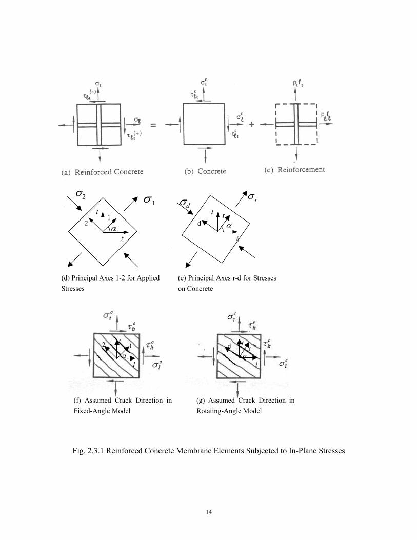
Fig. 2.3.1 Reinforced Concrete Membrane Elements Subjected to In-Plane Stresses..............................................................................................14

(a) Reinforced Concrete .........................................................................14 (b) Concrete ............................................................................................14 (c) Reinforcement...................................................................................14 (d) Principal Axes 1-2 for Applied Stresses ...........................................14 (e) Principal Axes r-d for Stresses on Concrete .....................................14 (f) Assumed Crack Direction in Fixed-Angle Model ............................14 (g) Assumed Crack Direction in Rotating-Angle Model........................14

Fig. 2.3.2 Constitutive Laws of Concrete in Tension and Compression .......................24 Fig. 2.3.3 Constitutive Law of Steel Bars......................................................................25 Fig. 2.3.4 Flow Chart of Solution Procedure for Softened Membrane Model ..............26 Fig. 3.1.1 Arrangement of Reinforcement in Trial Panel TE-2 .....................................30 Fig. 3.1.2 Crack Pattern of Trial Panel TE-2 at 2% Tensile Strain................................31 Fig. 3.3.1 Formwork for Crack Simulation Tests (TSB1 to TSB5)...............................34 Fig. 3.3.2 Formwork for Crack Simulation Tests (TSB6 to TSB10).............................34 Fig. 3.3.3 Dimensions of U-Shape Inserts (Unit: in.) ....................................................36

(a) Perspective View ..............................................................................36 (b) Top View ..........................................................................................36 (c) Side View..........................................................................................36

Fig. 3.3.4 Specimens after Casting Concrete.................................................................37 Fig. 3.3.5 Tendon Jacking System.................................................................................39 Fig. 3.4.1 Stress-Strain Curve of Bare Strands ..............................................................41 Fig. 3.5.1 Test Setup for a Typical Specimen................................................................42 Fig. 3.6.1 Crack Patterns of Specimens TSB2 and TSB3..............................................43

(a) TSB2-North.......................................................................................43 (b) TSB3-North.......................................................................................43

Fig. 3.6.2 Crack Patterns of Specimens TSB6 and TSB8..............................................44 (a) TSB6-South.......................................................................................44 (b) TSB8-South.......................................................................................44

Fig. 4.2.1 Steel Layout and Dimensions of Test Panels in Group TE ...........................50 (a) Steel Layout and Dimensions of Panels TE-4, 3, and 5....................50 (b) Steel Layout and Dimensions of Panel TE-6....................................51 (c) Steel Layout and Dimensions of Panel TE-7....................................52

Fig. 4.2.2 Formworks of Panels in Group TE................................................................54 (a) Formwork of Panel TE-4 ..................................................................54

xiii

(b) Formwork of Panel TE-6 ..................................................................54 (c) Formwork of Panel TE-7 ..................................................................55

Fig. 4.2.3 Special Steel Jig.............................................................................................55 Fig. 4.3.1 Typical Stress-Strain Curve from Concrete Cylinder Compression Test..........................................................................................................57 Fig. 4.4.1 Sequential Loading Path used in Group TE ..................................................58 Fig. 4.5.1 11 εσ − Relationships of Panels TE-4, 3, and 5..............................................60 Fig. 4.5.2 11 εσ − Relationships of Panels TE-6, 3, and 7..............................................60 Fig. 4.5.3 22 εσ − Relationships of Panels TE-4, 3, and 5 .............................................61 Fig. 4.5.4 22 εσ − Relationships of Panels TE-6, 3, and 7 .............................................62 Fig. 4.6.1 Experimental cc εσ − Relationships of Concrete in Decompression ...........64 Fig. 4.6.2 Experimental Smeared (Average) Tensile Stress-Strain Curves of

Concrete .....................................................................................................65 Fig. 4.6.3 Smeared Stress-Strain Relationships of Concrete in Tension .......................67 Fig. 4.6.4 Smeared (Average) Stress-Strain Relationships of Concrete in

Tension (TE-3)...........................................................................................68 Fig. 4.6.5 Smeared (Average) Stress-Strain Relationships of Concrete in




Tension (TE-7)...........................................................................................70 Fig. 4.7.1 Comparison of Experimental Stress-Strain Curve of Prestressing

Tendons Embedded in Concrete in Panel TE-4 with that of Bare Strands........................................................................................................72

Fig. 4.7.2 Comparison of Theoretical Smeared (Average) Stress-Strain Curve of Prestressing Tendons with Experimental Curve for Panel

TE-4...........................................................................................................74 Fig. 4.7.3 Comparison of Theoretical Smeared (Average) Stress-Strain

Curve of Prestressing Tendons with Experimental Curve for Panel TE-3...........................................................................................................74 Fig. 4.7.4 Comparison of Theoretical Smeared (Average) Stress-Strain



Curve of Prestressing Tendons with Experimental Curve for Panel TE-7...........................................................................................................76 Fig. 4.8.1 Smeared (Average) Stress-Strain Relationships of Concrete in

Compression in Panels TE-4, 3, and 5.......................................................77

xiv

Fig. 4.8.2 Smeared (Average) Stress-Strain Relationships of Concrete in Compression in Panels TE-6, 3, and 7.......................................................78

Fig. 4.8.3 Crack Pattern of Panel TE-6..........................................................................81 Fig. 4.8.4 Crack Pattern of Panel TE-3..........................................................................81 Fig. 5.2.1 Steel Layout and Dimensions of Test Panels in Group TA...........................85

(a) Steel Layout and Dimensions of Panels TA-1, 2, 3, and 4 ...............85 (b) Steel Layout and Dimensions of Panel TE-5....................................86

Fig. 5.2.2 Dimensions of V-Shape Inserts (Unit: in.) ....................................................88 (a) Perspective View ..............................................................................88 (b) Top View ..........................................................................................88 (c) Bearing Plate.....................................................................................88

Fig. 5.2.3 Formworks of Panels in Group TA ...............................................................89 (a) Formwork of Panel TA-3..................................................................89 (b) Formwork of Panel TA-5..................................................................89

Fig. 5.2.4 Tendon Jacking System for Panels in Group TA ..........................................91 (a) Setup of Pulling End .........................................................................91 (b) Details of Supporting Chair ..............................................................91

Fig. 5.3.1 Stress-Strain Curves of Bare Steel Bars ........................................................93 Fig. 5.4.1 Proportional Loading Path used in Group TA...............................................94 Fig. 5.5.1 Shear Stress-Strain Curves of Panels TA-1, 2, and 3 ....................................96 Fig. 5.5.2 Shear Stress-Strain Curves of Panels TA-2, 4, and 5 ....................................96 Fig. 5.5.3 Shear Stress vs. Principal Tensile Strain Curves of Panels TA-1, 2, and 3..............................................................................................................99 Fig. 5.5.4 Shear Stress vs. Principal Tensile Strain Curves of Panels TA-2, 4, and 5............................................................................................................100 Fig. 5.5.5 Shear Stress vs. Principal Compressive Strain Curves of Panels

TA-1, 2, and 3 .............................................................................................101 Fig. 5.5.6 Shear Stress vs. Principal Compressive Strain Curves of Panels

TA-2, 4, and 5 .............................................................................................102 Fig. 5.6.1 Experimental Concrete Compressive Stress-Strain Curves of Panels

TA-1, 2, and 3 .............................................................................................104 Fig. 5.6.2 Experimental Concrete Compressive Stress-Strain Curves of Panels

TA-2, 4, and 5 .............................................................................................104 Fig. 5.6.3 Constitutive Laws of Concrete in Compression ..........................................106 Fig. 5.6.4 ( )βf versus β Relationships for Reinforced and Prestressed Concrete Panels............................................................................................108 Fig. 5.6.5 pW versus β Relationships for Prestressed Concrete Panels.....................110 Fig. 5.6.6 Comparison of SMM-PC predicted Concrete Compressive

Stress-Strain Curves with Experimental Data of Panels TA-1 to TA-5 ...............................................................................................111

Fig. 6.2.1 Coordinate System in a Prestressed Concrete Membrane Element.............116 (a) Prestressed Concrete ...................................................................... 116 (b) Concrete ..........................................................................................116 (c) Reinforcement.................................................................................116 (d) Prestressed Concrete Element.........................................................116 (e) Principal Coordinate 2-1 for Applied Stresses................................116

xv

Fig. 6.2.2 Flow Chart of Solution Procedure for SMM-PC.........................................123 Fig. 6.3.1 Applied Shear Stress tlτ versus Shear Strain tlγ of Panel TA-1................124 Fig. 6.3.2 Applied Shear Stress tlτ versus Shear Strain tlγ of Panel TA-2................125 Fig. 6.3.3 Applied Shear Stress tlτ versus Shear Strain tlγ of Panel TA-3................125 Fig. 6.3.4 Applied Shear Stress tlτ versus Shear Strain tlγ of Panel TA-4................126 Fig. 6.3.5 Applied Shear Stress tlτ versus Shear Strain tlγ of Panel TA-5................126 Fig. 7.2.1 Cross Section of Type-A Beams .................................................................131

(a) Cross Section of Beams B1, B2, and B4 ........................................131 (b) Cross Section of Beams B3 and B5 ................................................132

Fig. 7.2.2 Elevation and Reinforcement Details of Beam B1......................................133 Fig. 7.2.3 Elevation and Reinforcement Details of Beams B2 and B3........................133 Fig. 7.2.4 Elevation and Reinforcement Details of Beams B4 and B5........................134 Fig. 7.3.1 Reinforcement and Instrumentation Details of Beams B1, B2,

and B3 (Web Shear Specimens) ................................................................ 135 (a) Beam B1..........................................................................................135 (b) Beam B2..........................................................................................136 (c) Beam B3..........................................................................................136

Fig. 7.3.2 Reinforcement and Instrumentation Details of Beams B4 and B5 (Flexural Shear Specimens) ....................................................................... 137

(a) Beam B4..........................................................................................137 (b) Beam B5..........................................................................................137

Fig. 7.4.1 Casting of Test Specimens ..........................................................................138 (a) Concrete Placed in Beam B4 by a Hopper......................................138 (b) Compaction using Needle Vibrators in Beam B4...........................139 (c) Removal of Anchors of Hold-down Rod from Beam B3 ...............139

Fig. 7.5.1 Test Setup ....................................................................................................140 Fig. 7.5.2 Loading Positions of Beams ........................................................................142

(a) Loading Point and LVDT Locations for Beams B1, B2, and B3 ...142 (b) Loading Point and LVDT Locations for Beams B4 and B5...........142

Fig. 7.5.3 LVDT Setup on Beam B4 ...........................................................................143 Fig. 7.5.4 Location of Strain Gages on L Bars in Beam B1 ........................................144 Fig. 7.5.5 Location of Strain Gages on R Bars in Beams B2 and B3 ..........................144 Fig. 7.5.6 Location of Strain Gages on L Bars in Beams B4 and B5 ..........................145 Fig. 7.5.7 Tracking and Measuring Shear Cracks on the Web of Beam B4................145 Fig. 7.6.1 Load Deformation Curves of the Specimens B1 to B5 ...............................147 Fig. 8.2.1 Analytical Model used for Calculating Web Shear Capacities of Beams ...150 Fig. 8.2.2 Variation of Normalized Concrete Shear of Beams Tested in Web Shear............................................................................................................154 Fig. 8.2.3 Determination of Number of Stirrups for “Contribution of Steel” Vs.........154

(a) Average Spacing Method................................................................154 (b) Minimum Shear Resistance Method...............................................154

Fig. 9.1.1 Details of Beams Tested by Other Researchers...........................................156 (a) Cross Section of Beams Tested by Lyngberg .................................156 (b) Elevation of Beams Tested by Lyngberg........................................156 (c) Cross Section of Beams Tested by Rangan ....................................157

xvi

(d) Elevation of Beams Tested by Rangan ...........................................157 (e) Details of CI Specimens Tested by Elzanaty..................................158 (f) Details of CW Specimens Tested by Elzanaty ...............................158

Fig. 9.1.2 Variation of Normalized Concrete Shear with a/d ......................................159 Fig. 9.1.3 Variation of Normalized Ultimate Shear Capacities of Beams with a/d.....160 Fig. 9.3.1 Layout of Girders and Roadway Slab considered in Design Examples ......165 Fig. 9.3.2 Dimensional Details of Beam and Overlaying Slab....................................165

xvii

LIST OF TABLES

Page Table 3.2.1 Variables of 10 Specimens ..................................................................... 32 Table 3.4.1 Mechanical Properties of Steel Bars............................................................41 Table 3.6.1 Average Crack Spacing of 10 Specimens....................................................45 Table 4.1.1 Two Variables of Test Panels in Group TE.................................................48 Table 4.8.1 Experimental Softening Coefficients...........................................................79 Table 4.8.2 Comparison of Experimental Softening Coefficients with Analytical Model...........................................................................................................80 Table 5.1.1 Principal Variables of Test Panels in Group TA .........................................84 Table 5.3.1 Mechanical Properties of Steel Bars............................................................92 Table 5.6.1 Calculation of β and ( )βf for Prestressed Concrete Panels ...................107 Table 5.6.2 Calculation of pW for Prestressed Concrete Panels ..................................109 Table 7.2.1 Test Specimens .........................................................................................130 Table 7.6.1 Failure Loads of Beams ............................................................................146 Table 7.6.2 Experimental Ultimate Strains in Specimens B1 to B5 measured by LVDTs................................................................................................147 Table 7.6.3 Experimental Ultimate Strains in Strain Gages for Specimens B1 to B5.............................................................................................................148 Table 8.2.1 Angles of Failure Planes Corresponding to Beam Shear

Capacities as per Model ...........................................................................153 Table 8.2.2 Normalized Concrete Shear Contributions of Beams B1 through B3 .....154 Table 9.2.1 Comparison of Test Results for UH Specimens ......................................162 Table 9.2.2 Comparison of Test Results for Lyngberg’s Specimens .........................162 Table 9.2.3 Comparison of Test Results for Rangan’s Specimens.............................163 Table 9.2.4 Comparison of Test Results for Elzanaty’s Specimens ...........................164 Table 9.3.1 Beam Design 1.........................................................................................167 Table 9.3.2 Beam Design 2.........................................................................................169 Table 9.3.3 Beam Design 3.........................................................................................172 Table 9.3.4 Beam Design 4.........................................................................................174 Table 9.4.1 Design of Non-Prestressed Beam ............................................................177

xviii

NOTATIONS

1 = direction of applied principal tensile stress 2 = direction of applied principal compressive stress a = shear span of prestressed beams A = cross-sectional areas of prestressed beams

cA = cross-sectional areas of concrete

vA = cross-sectional areas of single stirrup in prestressed beam

psA = cross-sectional areas of prestressing tendons

inclA = cross-sectional areas of prestressing beams along failure plane

wb = width of web of prestressed I-beams

c = constant in stress-strain relationship of concrete after cracking d = depth of c.g.s. of tendons from top concrete fiber in prestressed beams

bvd = diameter of stirrups used in prestressed beams

−d = direction of principal compressive stress of concrete

cE = elastic modulus of concrete

cE ′ = decompression modulus of concrete, given as 02 εcf ′

cE ′′ = modulus of concrete in tension before cracking

psE = modulus of elasticity of prestressing strands

psE ′ = modulus of bare prestressing strands in inelastic stage

psE ′′ = modulus of prestressing tendons embedded in concrete in inelastic stage

sE = modulus of elasticity of mild steel bars

cf ′ = cylinder compressive strength of concrete

cf ′ = square root of cylinder compressive strength of concrete (same units as cf ′ )

xix

crf = cracking tensile strength of concrete

lf = smeared (average) stress in longitudinal steel bars

pf l = smeared (average) stress in longitudinal prestressing tendons

nf = apparent yield strength of mild steel bars embedded in concrete

pf = smeared (average) stress in mild steel bars at peak

pif = initial stress of prestressing tendons

psf = stress of prestressing tendons

puf = stress in prestressing tendons at nominal strength

puf ′ = revised ultimate strength of prestressing tendons

sf = smeared (average) stress in mild steel bars, becomes lf or tf when applied

to longitudinal and transverse steel, respectively

tf = smeared (average) stress in transverse steel bars

tpf = smeared (average) stress in transverse prestressing tendons

yf = yield strength of bare mild steel bars

G = shear modulus of concrete h = depth of prestressed beam H = tensile load or strain to represent load stages in crack simulation tests

rK = reduction factor for concrete contribution in non-prestressed concrete

l = direction of longitudinal reinforcements

nL = span of prestressed beam

m = constant in stress-strain relationships of prestressing tendons M = bending moment at design section of prestressed beams P = total tensile load on panels r = direction of principal tensile stress of concrete t = direction of transverse reinforcements s = spacing of stirrups in prestressed beams

xx

S = shear force along failure plane in prestressed beams T = tensile force in tendons in prestressed beams

∑ VF = summation of stirrup forces lying on the failure plane in prestressed beams

V = shear capacity of prestressed beams

calV = shear capacity of prestressed beams calculated from shear theory

expV = experimental shear capacity of beams

cV = concrete contribution in shear resistance of beams

sV = steel contribution in shear resistance of beams

uV = design shear force acting on beams

max.cV = maximum concrete shear capacity in beams

max.uV = maximum design shear capacity of beams

uw = uniformly distributed load acting on beams

pW = prestress factor in softening coefficient

x = distance of design section from support of prestressed beam α = angle of the principal tensile stress of concrete ( −r axis) with respect to the

longitudinal steel bars ( −l axis)

1α = angle of the applied principal tensile stress ( −1 axis) with respect to the

longitudinal steel bars ( −l axis)

β = deviation angle of the direction of concrete principal tensile stress ( −r axis)

and the direction of −1 axis, 1αα −

tlγ = smeared (average) shear strain in t−l coordinates

hvγ = smeared (average) shear strain in horizontal-vertical plane in beam tests

12γ = smeared (average) shear strain in 21− coordinates

0ε = concrete cylinder strain corresponding to peak cylinder strength, cf ′

xxi

1ε = biaxial smeared (average) principal strain in −1 direction

hε = smeared (average) horizontal strain in beam tests

vε = smeared (average) vertical strain in beam tests

dε = smeared (average) diagonal strain in beam tests

1Hε = ultimate strain recorded in LVDT H1 during beam tests

2Hε = ultimate strain recorded in LVDT H2 during beam tests

1Vε = ultimate strain recorded in LVDT V1 during beam tests

2Vε = ultimate strain recorded in LVDT V2 during beam tests

1Dε = ultimate strain recorded in LVDT D1 during beam tests

2Dε = ultimate strain recorded in LVDT D2 during beam tests

1SGε = ultimate strain recorded in strain gage SG1 during beam tests




1ε = uniaxial smeared (average) principal strain in −1 direction

2ε = biaxial smeared (average) principal strain in −2 direction

2ε = uniaxial smeared (average) principal strain in −2 direction

cε = uniaxial strain in concrete

ciε = initial strain in concrete

crε = concrete cracking strain taken as 0.00008

xxii

cxε = extra strain in concrete after decompression

dε = smeared (average) concrete compressive strain in concrete principal

−d direction

lε = biaxial smeared (average) strain in the direction of longitudinal steel bars

( −l axis)

lε = uniaxial smeared (average) strain in the direction of longitudinal steel bars

( −l axis)

nε = uniaxial smeared (average) yielding strain of steel bars embedded in

concrete

pε = uniaxial smeared (average) strain in mild steel at peak

piε = initial uniaxial strain of prestressing tendons

rε = smeared (average) concrete tensile strain in concrete principal −r direction

sε = smeared (average) strain in mild steel, sε becomes lε or tε , when applied

to the longitudinal or transverse steel, respectively

sfε = smeared (average) strain of steel bars which yields first, taking into account

the Hsu/Zhu ratios

tε = biaxial smeared (average) strain in the direction of transverse steel bars

( −t axis)

tε = uniaxial smeared (average) strain in the direction of transverse steel bars

( −t axis)

yε = yielding strain in bare steel bars

φ = angle between the horizontal and the diagonal LVDTs in beam tests

ζ = softening coefficient

εζ = strain softening coefficient

xxiii

σζ = stress softening coefficient

η = reinforcement index, taken as ( ) ( )lll σρσρ −− yttyt ff

η′ = η or its reciprocal whichever is less than unity

12ν = Hsu/Zhu ratio (increment of strain in −1 direction due to a strain in

−2 direction)

21ν = Hsu/Zhu ratio (increment of strain in −2 direction due to a strain in

−1 direction)

lρ = longitudinal steel ratio

plρ = longitudinal prestressing steel ratio

tρ = transverse steel ratio

1σ = applied principal stress in −1 direction

c1σ = smeared (average) concrete stress in −1 direction

2σ = applied principal stress in −2 direction

c2σ = smeared (average) concrete stress in −2 direction

cσ = smeared (average) stress in concrete

ciσ = initial compressive stress in concrete due to prestress

dσ = smeared (average) compressive stress in concrete principal −d direction

lσ = applied normal stress in −l direction

pσ = prestress on concrete

pkσ = peak compressive stress on panels in vertical direction

rσ = smeared (average) tensile stress in concrete principal −r direction

xxiv

tσ = applied normal stress in −t direction

c12τ = smeared shear stress of cracked concrete in 21− coordinates

tlτ = applied shear stress in t−l coordinates

1

CHAPTER 1

INTRODUCTION

1.1 Overview of Research The idea of prestressing concrete structures was first applied in 1928 by Eugene Freyssinet

(1956) in his effort to save the Le Veurdre Bridge over the Allier River near Vichy, France. The primary purpose of using prestressed concrete was to eliminate/reduce cracking at service load and to fully utilize the capacity of high-strength steel. After the Second World War, prestressed concrete became prevalent due to the needs of reconstruction and the availability of high-strength steel. Today, prestressed concrete has become the predominant material in highway bridge construction. It is also widely used in the construction of buildings, underground structures, TV towers, floating storages and offshore structures, power stations, nuclear reactor vessels, etc.

This research intends to solve one of the most troublesome problems in prestressed concrete, namely shear. The problem arises from the lack of a rational model to predict the behavior of prestressed concrete structures under shear action and the various modes of shear failures. Because of this deficiency, all the guidelines for shear design, such as ACI Codes and AASHTO Specifications, are empirical and have severe limitations.

Hsu (2002) pointed out the deficiency in the shear design guidelines for reinforced and prestressed concrete bridge girders. By comparing the fixed-angle model with the rotating-angle model, he showed that the “concrete contribution” Vc for the shear resistance can be derived from the shear resistance of cracked concrete, rather than from the tensile strength of concrete as assumed in ACI Codes (2005) or the tensile stress of cracked concrete in AASHTO Specifications (2004).

In Loov’s “shear friction” theory (Loov, 1978, 1997, and 2002) for girders, Vc was derived from the shear resistance of cracked concrete along a shear failure plane. Based on the “shear friction” principle, Loov established a shear design method and illustrated it with a detailed example. However, the determination of Vc by a “shear friction” principle was not widely accepted. Hsu (2002) noted that Loov’s method can be modified and be applicable to prestressed concrete girders, as long as the constitutive laws of prestressed concrete membrane elements are clarified. These constitutive laws would allow us to understand the effect of prestress on the “concrete contribution” Vc.

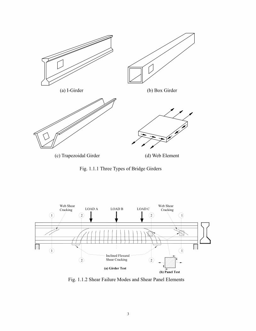
Similar to reinforced concrete structures, wall-type or shell-type prestressed concrete structures can be visualized as assemblies of membrane elements subjected to normal and shear stresses in the plane of elements. Taking bridge girders as examples, Fig. 1.1.1(a) to (c) show three main types of prestressed bridge girders: I-girder, box girder, and trapezoidal girder. The webs of the girders, which are shear-governed, can be analyzed using finite element methods if there is a rational shear model for plane stress elements (Fig. 1.1.1(d)). Therefore, the key to

2

solving the shear problem of prestressed concrete structures is to thoroughly understand the shear behavior of prestressed concrete membrane elements.

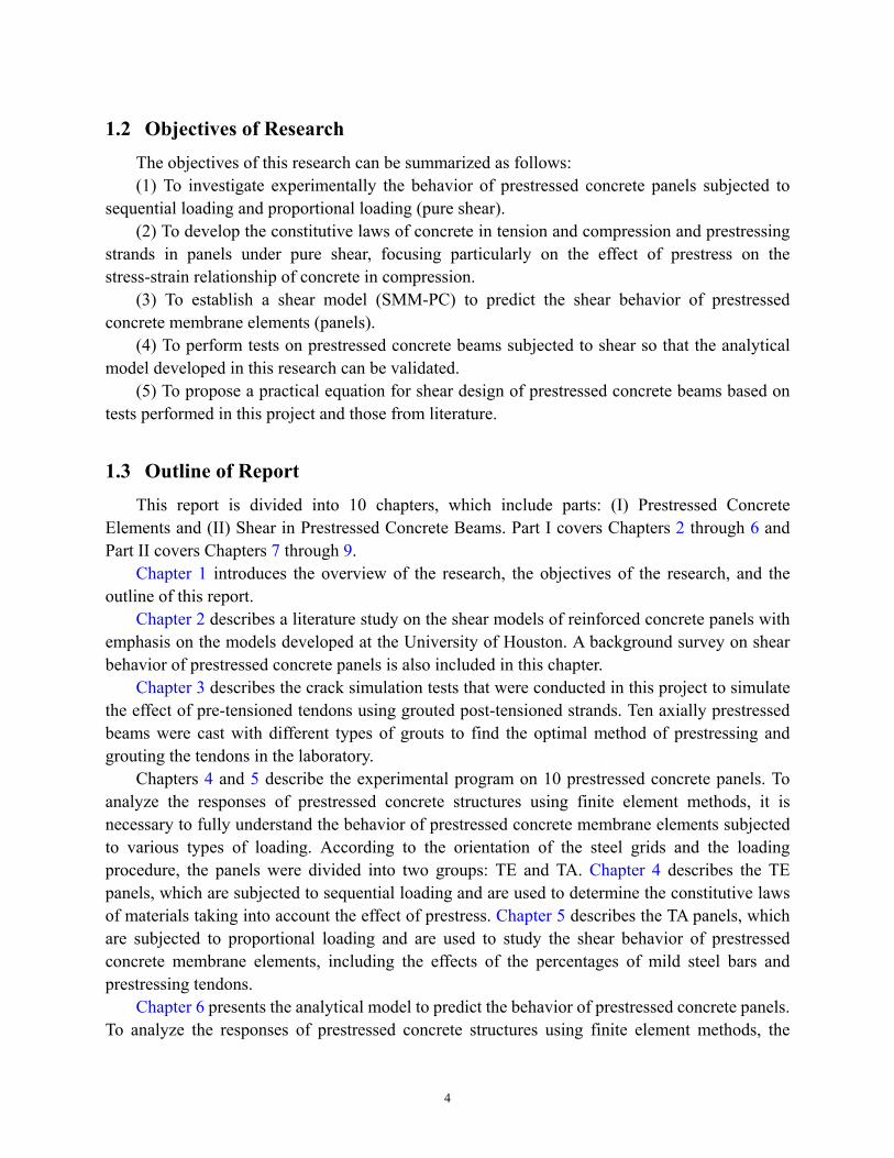
Figure 1.1.2(a) shows a typical I-girder used in highway bridges. The girder may encounter two major kinds of shear failure modes: (1) web shear failure near the supports where the shear force is large and the bending moment is small, and (2) flexural-shear failure near the one-third or quarter point of the span where both the shear force and the bending moment are large. A typical membrane element subjected to in-plane stresses can be isolated from the failure region of the girder, as shown in Fig. 1.1.2(b). The research in this project focuses on the shear behavior of prestressed concrete membrane elements (panels).

Many researchers have developed various types of analytical models of reinforced concrete, such as truss models, orthotropic models, nonlinear elastic models, plastic models, micro models, etc. As compared with the other models, the orthotropic model stands out both in accuracy and in efficiency. Over the past 20 years, extensive experimental and theoretical studies on the shear behavior of reinforced concrete have been carried out by a research group at the University of Houston (UH). A series of analytical models was established to predict the nonlinear shear behavior of reinforced concrete membrane elements. These models are: the Rotating-Angle Softened Truss Model (RA-STM) by Hsu (1993), Belarbi and Hsu (1995), and Pang and Hsu (1995); the Fixed-Angle Softened Truss Model (FA-STM) by Pang and Hsu (1996) and Hsu and Zhang (1997); and the Softened Membrane Model (SMM) by Hsu and Zhu (2002). All these models are rational because they satisfy Navier’s three principles of mechanics of materials: stress equilibrium, strain compatibility, and constitutive relationships of materials.

The Softened Membrane Model has been proven to be successful in predicting the entire shear behavior of reinforced concrete panels including both the pre-peak and the post-peak regions. In this research, the SMM is extended to prestressed concrete panels. Ten prestressed concrete panels were tested to obtain the constitutive laws of concrete and prestressing strands. These constitutive laws, which take into account the effect of prestress, were then incorporated into the SMM. The new model established in this dissertation will be called the Softened Membrane Model for Prestressed Concrete (SMM-PC).

Another major part of this project involved development of a new simple shear design equation for girders. For this a series of five prestressed concrete I-beams were designed, cast, and tested to study their behavior in web shear as well as flexural shear failure modes. The results obtained from these tests were analyzed and a new simple equation was developed for the shear design of prestressed concrete girders. Results from other tests available in the literature (Lyngberg, 1976; Elzanaty et al., 1986; and Rangan, 1991) were used to verify the new design equation and make necessary modifications to the same. The new design equation was also extended to include non-prestressed girders.

3

LOAD A LOAD B LOAD C

1

1

2

2 12

1

2Shear CrackingInclined Flexural

Web ShearCracking Cracking

Web Shear

(a) Girder Test(b) Panel Test

Fig. 1.1.2 Shear Failure Modes and Shear Panel Elements

Fig. 1.1.1 Three Types of Bridge Girders

(a) I-Girder (b) Box Girder

(c) Trapezoidal Girder (d) Web Element

4

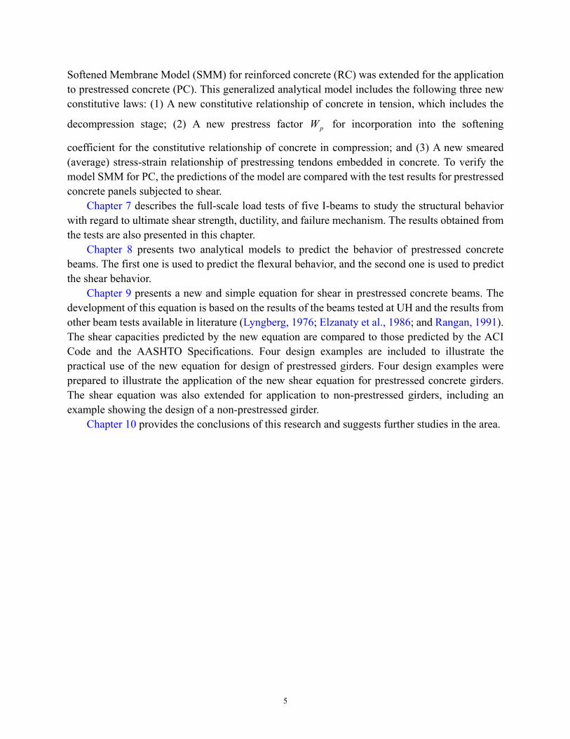
1.2 Objectives of Research The objectives of this research can be summarized as follows: (1) To investigate experimentally the behavior of prestressed concrete panels subjected to

sequential loading and proportional loading (pure shear). (2) To develop the constitutive laws of concrete in tension and compression and prestressing

strands in panels under pure shear, focusing particularly on the effect of prestress on the stress-strain relationship of concrete in compression.

(3) To establish a shear model (SMM-PC) to predict the shear behavior of prestressed concrete membrane elements (panels).

(4) To perform tests on prestressed concrete beams subjected to shear so that the analytical model developed in this research can be validated.

(5) To propose a practical equation for shear design of prestressed concrete beams based on tests performed in this project and those from literature.

1.3 Outline of Report This report is divided into 10 chapters, which include parts: (I) Prestressed Concrete

Elements and (II) Shear in Prestressed Concrete Beams. Part I covers Chapters 2 through 6 and Part II covers Chapters 7 through 9.

Chapter 1 introduces the overview of the research, the objectives of the research, and the outline of this report.

Chapter 2 describes a literature study on the shear models of reinforced concrete panels with emphasis on the models developed at the University of Houston. A background survey on shear behavior of prestressed concrete panels is also included in this chapter.

Chapter 3 describes the crack simulation tests that were conducted in this project to simulate the effect of pre-tensioned tendons using grouted post-tensioned strands. Ten axially prestressed beams were cast with different types of grouts to find the optimal method of prestressing and grouting the tendons in the laboratory.

Chapters 4 and 5 describe the experimental program on 10 prestressed concrete panels. To analyze the responses of prestressed concrete structures using finite element methods, it is necessary to fully understand the behavior of prestressed concrete membrane elements subjected to various types of loading. According to the orientation of the steel grids and the loading procedure, the panels were divided into two groups: TE and TA. Chapter 4 describes the TE panels, which are subjected to sequential loading and are used to determine the constitutive laws of materials taking into account the effect of prestress. Chapter 5 describes the TA panels, which are subjected to proportional loading and are used to study the shear behavior of prestressed concrete membrane elements, including the effects of the percentages of mild steel bars and prestressing tendons.

Chapter 6 presents the analytical model to predict the behavior of prestressed concrete panels. To analyze the responses of prestressed concrete structures using finite element methods, the

5

Softened Membrane Model (SMM) for reinforced concrete (RC) was extended for the application to prestressed concrete (PC). This generalized analytical model includes the following three new constitutive laws: (1) A new constitutive relationship of concrete in tension, which includes the

decompression stage; (2) A new prestress factor pW for incorporation into the softening

coefficient for the constitutive relationship of concrete in compression; and (3) A new smeared (average) stress-strain relationship of prestressing tendons embedded in concrete. To verify the model SMM for PC, the predictions of the model are compared with the test results for prestressed concrete panels subjected to shear.

Chapter 7 describes the full-scale load tests of five I-beams to study the structural behavior with regard to ultimate shear strength, ductility, and failure mechanism. The results obtained from the tests are also presented in this chapter.

Chapter 8 presents two analytical models to predict the behavior of prestressed concrete beams. The first one is used to predict the flexural behavior, and the second one is used to predict the shear behavior.

Chapter 9 presents a new and simple equation for shear in prestressed concrete beams. The development of this equation is based on the results of the beams tested at UH and the results from other beam tests available in literature (Lyngberg, 1976; Elzanaty et al., 1986; and Rangan, 1991). The shear capacities predicted by the new equation are compared to those predicted by the ACI Code and the AASHTO Specifications. Four design examples are included to illustrate the practical use of the new equation for design of prestressed girders. Four design examples were prepared to illustrate the application of the new shear equation for prestressed concrete girders. The shear equation was also extended for application to non-prestressed girders, including an example showing the design of a non-prestressed girder.

Chapter 10 provides the conclusions of this research and suggests further studies in the area.

PART I

PRESTRESSED CONCRETE ELEMENTS

8

9

CHAPTER 2

BACKGROUNDS ON SHEAR THEORIES OF REINFORCED AND

PRESTRESSEED CONCRETE PANELS

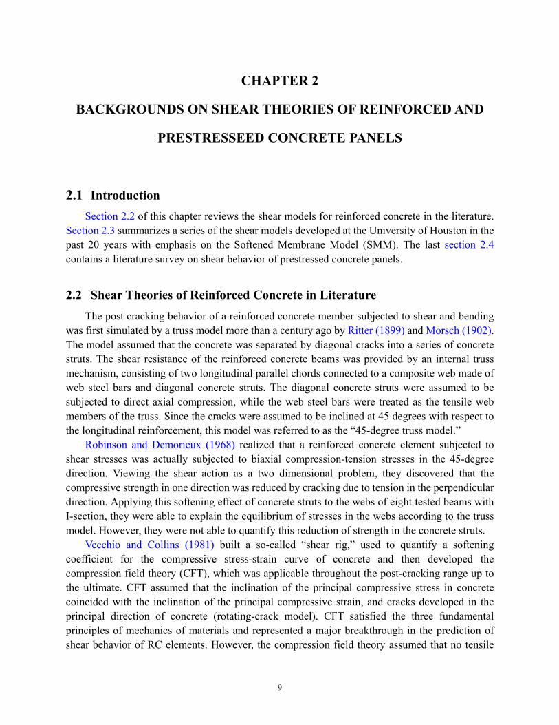
2.1 Introduction Section 2.2 of this chapter reviews the shear models for reinforced concrete in the literature.

Section 2.3 summarizes a series of the shear models developed at the University of Houston in the past 20 years with emphasis on the Softened Membrane Model (SMM). The last section 2.4 contains a literature survey on shear behavior of prestressed concrete panels.

2.2 Shear Theories of Reinforced Concrete in Literature The post cracking behavior of a reinforced concrete member subjected to shear and bending

was first simulated by a truss model more than a century ago by Ritter (1899) and Morsch (1902). The model assumed that the concrete was separated by diagonal cracks into a series of concrete struts. The shear resistance of the reinforced concrete beams was provided by an internal truss mechanism, consisting of two longitudinal parallel chords connected to a composite web made of web steel bars and diagonal concrete struts. The diagonal concrete struts were assumed to be subjected to direct axial compression, while the web steel bars were treated as the tensile web members of the truss. Since the cracks were assumed to be inclined at 45 degrees with respect to the longitudinal reinforcement, this model was referred to as the “45-degree truss model.”

Robinson and Demorieux (1968) realized that a reinforced concrete element subjected to shear stresses was actually subjected to biaxial compression-tension stresses in the 45-degree direction. Viewing the shear action as a two dimensional problem, they discovered that the compressive strength in one direction was reduced by cracking due to tension in the perpendicular direction. Applying this softening effect of concrete struts to the webs of eight tested beams with I-section, they were able to explain the equilibrium of stresses in the webs according to the truss model. However, they were not able to quantify this reduction of strength in the concrete struts.

Vecchio and Collins (1981) built a so-called “shear rig,” used to quantify a softening coefficient for the compressive stress-strain curve of concrete and then developed the compression field theory (CFT), which was applicable throughout the post-cracking range up to the ultimate. CFT assumed that the inclination of the principal compressive stress in concrete coincided with the inclination of the principal compressive strain, and cracks developed in the principal direction of concrete (rotating-crack model). CFT satisfied the three fundamental principles of mechanics of materials and represented a major breakthrough in the prediction of shear behavior of RC elements. However, the compression field theory assumed that no tensile

10

stress of concrete exists after cracking. This assumption is contradicted by many tests, which demonstrated that concrete stresses in tension increased significantly the stiffness of the cracked reinforced concrete structures. By taking into account the tensile strength of concrete, Vecchio and Collins (1986) further developed the modified compression field theory (MCFT) so it could predict the post-cracking stiffness. However, the theory had two deficiencies as pointed out by Hsu (1998). First, the MCFT violated the basic principle of mechanics by imposing concrete shear stresses in the principal directions. Second, it used the local stress-strain curve of steel bars embedded in concrete, rather than the smeared (average) stress-strain curves.

Balakrishnan and Murray (1988c) also applied a rotating crack model to predict the monotonic behavior of shear panels and deep beams using their own constitutive relationships (Balakrishnan and Murray, 1988a and 1988b). Poisson’s ratio was set to be zero when the concrete cracking began. The model was used to predict the behavior of a number of reinforced concrete panels tested by Vecchio and Collins (1982).

Crisfield and Wills (1989) performed analyses of a number of reinforced concrete panels tested by Vecchio and Collins (1982) using different material models. The models included a fixed crack model, a swinging-crack model, and a simple plasticity model. In the fixed crack model, the directions of orthogonal cracks were governed by the direction of the first principal stress that exceeded the tensile stress of the uncracked concrete. The swinging-crack model was a rotating crack model. The plasticity model had a square yield surface in compression in which no tension was allowed. The authors conducted extensive studies of the three proposed models on the panels and compared the analytical results with the experimental results. The authors also demonstrated the differences between the fixed crack and the swinging crack models.

A Rotating-Angle Softened Truss Model (RA-STM) was developed at the University of Houston (Belarbi and Hsu, 1994 and 1995; Pang and Hsu, 1995), which truly treated the cracked reinforced concrete as a smeared, continuous material. In this model, a new smeared (average) stress-strain curve of steel bars embedded in concrete (Belarbi and Hsu, 1994) was proposed. Moreover, a new algorithm was developed to significantly improve the iteration procedure in solving the 11 equilibrium, compatibility, and constitutive equations. As a result this model has two advantages. First, it produces a single and unique solution instead of multiple solutions as in the case of the modified compression field theory. Second, there is no need to perform the so-called “crack check,” which is difficult to apply in finite element methods.

These studies also showed that all theories that are based on rotating-angle could not logically produce the “concrete contribution” Vc because shear stresses could not exist along the rotating-angle cracks. In order to predict the “concrete contribution,” Hsu and his colleagues (Pang and Hsu, 1996; Hsu and Zhang, 1997; Zhang and Hsu, 1998) proposed the Fixed-Angle Softened Truss Model (FA-STM). In the FA-STM, the direction of cracks is assumed to be perpendicular to the applied principal tensile stresses at initial cracking rather than following the rotating cracks. The constitutive laws of concrete were set in the principal coordinate of the applied stresses at initial cracking. The only shortcoming of the FA-STM is that it is more complicated than the RA-STM because of the complexity in the stress-strain relationship of concrete in shear.

11

Ayoub and Filippou (1998) presented a rotating crack model that was an extension of the orthotropic models by Vecchio (1990) and Balakrishnan and Murray (1988a, 1988b, and 1988c). The panels tested by Vecchio and Collins (1982) were used in the correlation studies. Reasonable comparison was obtained between the analytical and experimental results.

Kaufmann and Marti (1998) proposed the Cracked Membrane Model (CMM), which was a combination of CFT (Vecchio and Collins, 1981) and a concrete tension stiffening model. The tension stiffening of concrete was modeled using a stepped, rigid-perfectly plastic concrete-steel bond slip relationship between the cracks with equilibrium maintained at the crack faces. Foster and Marti (2003) implemented the CMM into a finite element formulation and compared its predictions against experimental data from the shear panel tests by Meyboom (1987) and Zhang (1992).

Vecchio (2000 and 2001a) developed the Disturbed Stress Field Model (DSFM) based on the rotating crack model. The DSFM was a partially smeared model, which included shear slips along crack surfaces and required a “crack check” as in MCFT. The DSFM was more complicated when compared with the MCFT (Vecchio and Collins 1986). The predictions by the DSFM were compared to the experimental results of their panels and to the analytical results by MCFT (Vecchio et al., 2001b). The predictions using the DSFM and MCFT were found to be close in most cases.

Belletti et al. (2001) proposed a fixed crack model by adopting the stress-strain relationships of concrete and steel, aggregate interlock, and dowel action. The softening coefficient ζ proposed by Pang and Hsu (1995) was adopted in the model, which represented the softening effect of tensile strains on the perpendicular compression behavior of concrete. The panels tested at the University of Toronto (Vecchio and Collins 1982 and 1986; Collins et al., 1985; Bhide and Collins, 1989) and the panels tested at the University of Houston (Belarbi and Hsu, 1995; Pang and Hsu, 1995 and 1996; Hsu and Zhang, 1996) were analyzed. The predictions of the proposed model showed good agreement with the test results.

Although the rational models given above were able to predict the pre-peak behavior of shear elements, none of them could explain the existence of the post-peak load-deformation curves (descending branches). The Softened Membrane Model (SMM) (Hsu and Zhu, 2002) was therefore developed to predict the entire monotonic shear stress-strain curves of reinforced concrete panels including the descending branches. The capability of SMM to predict the descending branches was achieved by taking into account the Poisson effect (mutual effects of the two normal strains) of cracked reinforced concrete. This Poisson effect is characterized by two Hsu/Zhu ratios (Zhu and Hsu, 2002). In addition, a very simple stress-strain equation for concrete in shear was also derived using the equilibrium and compatibility equations and then incorporated in the model (Zhu, Hsu, and Lee, 2001). This new shear modulus significantly simplified the solution algorithm of fixed model theories, including SMM and FA-STM. It also increased the accuracy of these models.

To date, SMM has been proven to be capable of successfully predicting the entire behavior of RC panels under pure shear. In this research, SMM will be extended to predict the behavior of prestressed concrete panels.

12

2.3 Previous Studies by Research Group at UH In the past 20 years, Hsu and his colleagues performed over 130 panel tests using the

Universal Panel Tester (Hsu, Belarbi, and Pang, 1995) at the University of Houston. A series of three rational models for the monotonic shear behavior of the reinforced concrete elements (panels) was developed.

A reinforced concrete membrane element subjected to in-plane shear and normal stresses is shown in Fig. 2.3.1(a). The directions of the longitudinal and the transverse steel bars are designated as −l and −t axes, respectively, constituting the t−l coordinate system. The normal stresses are designated as σl and σt in the −l and the −t directions, respectively, and the shear stresses are represented by τlt in the t−l coordinate system. For Mohr’s circles, a positive shear stress τlt is the one that causes clockwise rotation of a reinforced concrete element (Hsu, 1993).

The applied principal stresses for the reinforced concrete element are defined as σ1 and σ2 based on the 21− coordinate system as shown in Fig. 2.3.1(d). The angle between the direction of the applied principal tensile stress ( −1 axis) and the direction of the longitudinal steel ( −l axis) is defined as the fixed-angle α1, because this angle does not change when the three in-plane stresses, σl, σt, and τlt, increase proportionally. This angle α1 is also called the steel bar angle because it defines the direction of the steel bars with respect to the applied principal stresses. The principal stresses in concrete coincide with the applied principal stresses σ1 and σ2 before

cracking. When the principal tensile stress 1σ reaches the tensile strength of concrete, cracks

will form and the concrete will be separated by the cracks into a series of concrete struts in the −2 direction as shown in Fig. 2.3.1(f). If the element is reinforced with different amounts of steel

in the −l and the −t directions, i.e., tt ff ρρ ≠ll in Fig. 2.3.1(c), the direction of the

principal stresses in concrete after cracking will deviate from the directions of the applied principal stresses. The new directions of the post-cracking principal stresses in concrete are defined by the dr − coordinate system shown in Fig. 2.3.1(e). Accordingly, the principal tensile stress and the principal compressive stress in the cracked concrete are defined as σr and σd, respectively.

The angle between the direction of the principal tensile stress in the cracked concrete ( −r axis) and the direction of the longitudinal steel ( −l axis) is defined as the rotating-angle α. The angle α is dependent on the relative amount of “smeared steel stresses,” ρlfl and ρtft, in the

longitudinal and the transverse directions as shown in Fig. 2.3.1(c). When tt ff ρρ >ll , the

dr − coordinate gradually rotates away from the 12 − coordinate and α becomes smaller with increasing load. With increasing applied proportional stresses (σl, σt, and τlt), the deviation between the angle α and the angle α1 increases. This deviation angle β is defined as α− α1. The

13

angle was determined by Hsu, Zhu and Lee (2001) for reinforced concrete and extended by Wang (2006) to prestressed concrete, as shown in Eq. 2.3-1.

( )

−

= −

21

121tan21

εεγ

β (2.3-1)

where ε1, ε2, and γ12 are the strains in the 21− coordinate of the applied principal stresses. When the percentages of reinforcement are the same in the −l and the −t directions, the rotating angle α is equal to the fixed-angle α1.

The Rotating-Angle Softened Truss Model is based on the assumption that the direction of cracks coincides with the direction of the principal compressive stress in the cracked concrete, as shown in Fig. 2.3.1(g). The derivations of all the equilibrium and compatibility equations are based on the rotating-angle α. In contrast, the Fixed-Angle Softened Truss Model is based on the assumption that the direction of the cracks coincides with the direction of the applied principal compressive stress as shown in Fig. 2.3.1(f). In the fixed-angle softened-truss model, all the equations are derived based on the fixed-angle α1.

The three stress components σl, σt, and τlt shown in Fig. 2.3.1(a) are the applied stresses on the reinforced concrete element viewed as a whole. The stresses on the concrete struts are denoted as

clσ , c

tσ , and ctlτ as shown in Fig. 2.3.1(b). The longitudinal and the transverse

14

Fig. 2.3.1 Reinforced Concrete Membrane Elements Subjected to In-Plane Stresses

dσ rσ

dr

l

tα

1 2

l

t

α1 l

t r d

α

(f) Assumed Crack Direction inFixed-Angle Model

(g) Assumed Crack Direction inRotating-Angle Model

2σ 1σ

2 1

l

t

1α

(d) Principal Axes 1-2 for AppliedStresses

(e) Principal Axes r-d for Stresseson Concrete

15

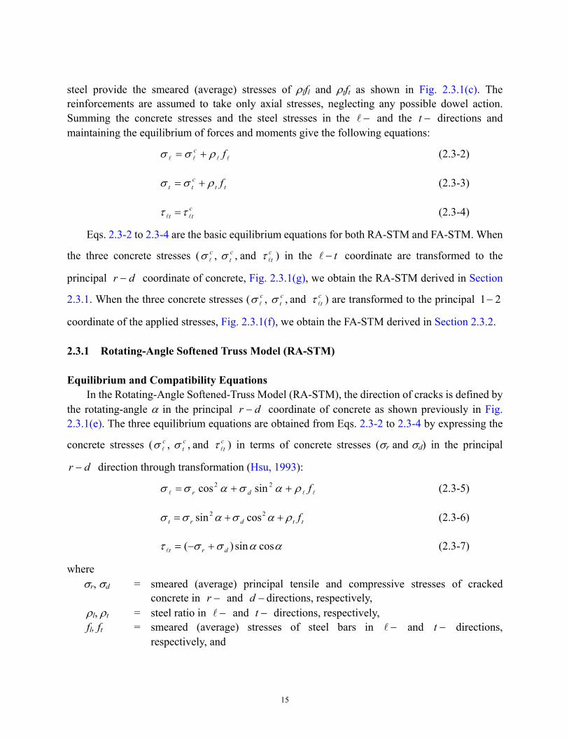
steel provide the smeared (average) stresses of ρlfl and ρtft as shown in Fig. 2.3.1(c). The reinforcements are assumed to take only axial stresses, neglecting any possible dowel action. Summing the concrete stresses and the steel stresses in the −l and the −t directions and maintaining the equilibrium of forces and moments give the following equations:

llll fc ρσσ += (2.3-2)

ttctt fρσσ += (2.3-3)

ctt ll ττ = (2.3-4)

Eqs. 2.3-2 to 2.3-4 are the basic equilibrium equations for both RA-STM and FA-STM. When

the three concrete stresses ( , , ct

c σσ l and ctlτ ) in the t−l coordinate are transformed to the

principal dr − coordinate of concrete, Fig. 2.3.1(g), we obtain the RA-STM derived in Section

2.3.1. When the three concrete stresses ( , , ct

c σσ l and ctlτ ) are transformed to the principal 21−

coordinate of the applied stresses, Fig. 2.3.1(f), we obtain the FA-STM derived in Section 2.3.2.

2.3.1 Rotating-Angle Softened Truss Model (RA-STM) Equilibrium and Compatibility Equations

In the Rotating-Angle Softened-Truss Model (RA-STM), the direction of cracks is defined by the rotating-angle α in the principal dr − coordinate of concrete as shown previously in Fig. 2.3.1(e). The three equilibrium equations are obtained from Eqs. 2.3-2 to 2.3-4 by expressing the

concrete stresses ( , , ct

c σσ l and ctlτ ) in terms of concrete stresses (σr and σd) in the principal

dr − direction through transformation (Hsu, 1993):

lll fdr ρασασσ ++= 22 sincos (2.3-5)

ttdrt fρασασσ ++= 22 cossin (2.3-6)

αασστ cossin)( drt +−=l (2.3-7)

where σr, σd = smeared (average) principal tensile and compressive stresses of cracked

concrete in −r and −d directions, respectively, ρl, ρt = steel ratio in −l and −t directions, respectively, fl, ft = smeared (average) stresses of steel bars in −l and −t directions,

respectively, and

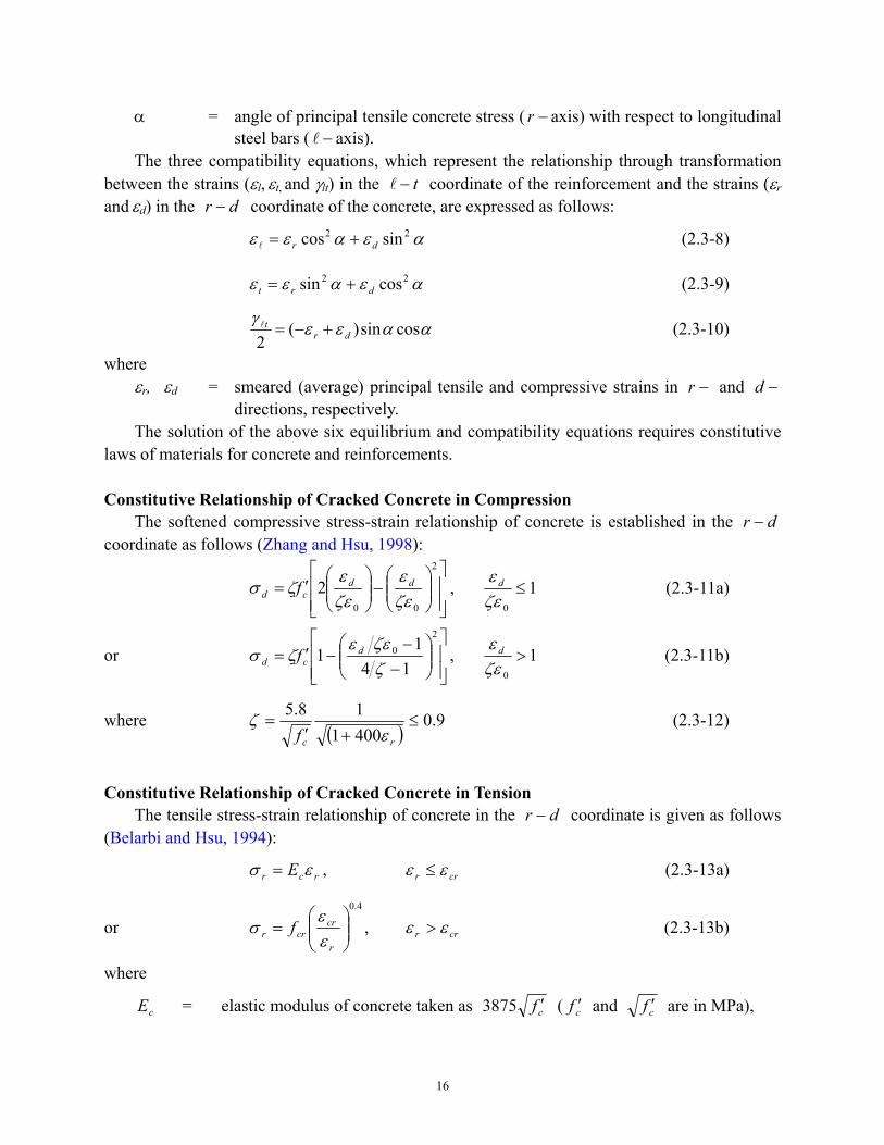
16

α = angle of principal tensile concrete stress ( −r axis) with respect to longitudinal steel bars ( −l axis).

The three compatibility equations, which represent the relationship through transformation between the strains (εl, εt, and γlt) in the t−l coordinate of the reinforcement and the strains (εr

and εd) in the dr − coordinate of the concrete, are expressed as follows:

αεαεε 22 sincos dr +=l (2.3-8)

αεαεε 22 cossin drt += (2.3-9)

ααεεγ cossin)(2 dr

t +−=l (2.3-10)

where εr, εd = smeared (average) principal tensile and compressive strains in −r and −d

directions, respectively. The solution of the above six equilibrium and compatibility equations requires constitutive

laws of materials for concrete and reinforcements.

Constitutive Relationship of Cracked Concrete in Compression The softened compressive stress-strain relationship of concrete is established in the dr −

coordinate as follows (Zhang and Hsu, 1998):

−

′=

2

00

2ζεε

ζεε

ζσ ddcd f , 1

0

≤ζεε d (2.3-11a)

or

−

−−′=

20

141

1ζζεε

ζσ dcd f , 1

0

>ζεε d (2.3-11b)

where ( )

9.0400118.5

≤+′

=rcf ε

ζ (2.3-12)

Constitutive Relationship of Cracked Concrete in Tension

The tensile stress-strain relationship of concrete in the dr − coordinate is given as follows (Belarbi and Hsu, 1994):

rcr E εσ = , crr εε ≤ (2.3-13a)

or 4.0

=

r

crcrr f

εε

σ , crr εε > (2.3-13b)

where

cE = elastic modulus of concrete taken as cf ′3875 ( cf ′ and cf ′ are in MPa),

17

εcr = concrete cracking strain taken as 0.00008, and

fcr = concrete cracking stress taken as cf ′31.0 ( cf ′ and cf ′ are in MPa).

Constitutive Relationship of Steel Bars Embedded in Cracked Concrete

The smeared (average) tensile stress-strain relationship of steel embedded in concrete in the t−l coordinate can be expressed as follows (Pang and Hsu, 1995):

sss Ef ε= , ns εε ≤ (2.3-14a)

++−=

y

sys BBff

εε

)25.002.0()291.0( , ns εε > (2.3-14b)

where )293.0( Byn −= εε (2.3-15)

and 5.1

1

=

y

cr

ff

Bρ

(2.3-16)

In the above equations, l replaces s in the subscript of symbols for the longitudinal steel, and t replaces s for the transverse steel.

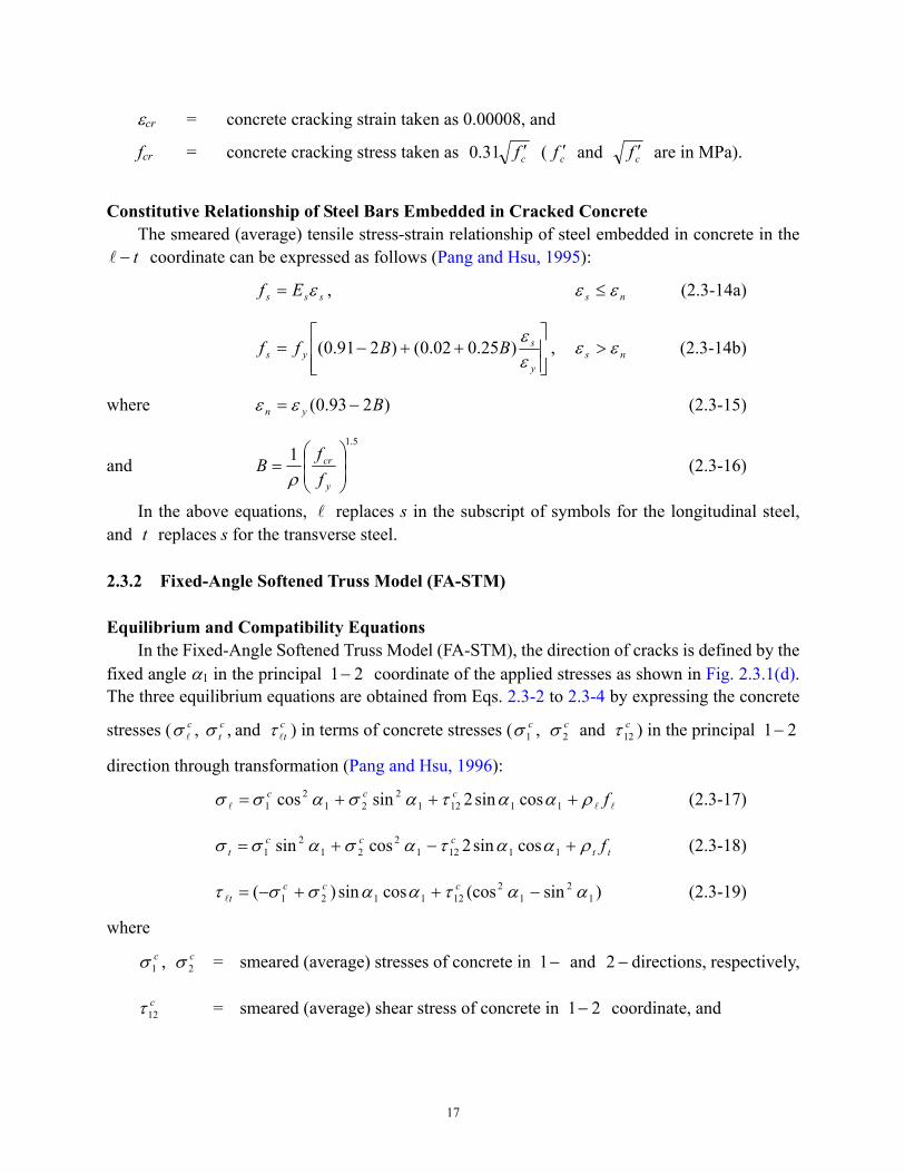
2.3.2 Fixed-Angle Softened Truss Model (FA-STM) Equilibrium and Compatibility Equations

In the Fixed-Angle Softened Truss Model (FA-STM), the direction of cracks is defined by the fixed angle α1 in the principal 21− coordinate of the applied stresses as shown in Fig. 2.3.1(d). The three equilibrium equations are obtained from Eqs. 2.3-2 to 2.3-4 by expressing the concrete

stresses ( , , ct

c σσ l and ctlτ ) in terms of concrete stresses ( c

1σ , c2σ and c

12τ ) in the principal 21−

direction through transformation (Pang and Hsu, 1996):

lll fccc ραατασασσ +++= 111212

212

1 cossin2sincos (2.3-17)

ttccc

t fραατασασσ +−+= 111212

212

1 cossin2cossin (2.3-18)

)sin(coscossin)( 12

12

121121 ααταασστ −++−= ccctl (2.3-19)

where c1σ , c

2σ = smeared (average) stresses of concrete in −1 and −2 directions, respectively,

c12τ = smeared (average) shear stress of concrete in 21− coordinate, and

18

α1 = angle of applied principal tensile stress ( −1 axis) with respect to longitudinal steel bars ( −l axis).

The three compatibility equations, which represent the relationship through transformation between the strains (εl, εt, and γlt) in the t−l coordinate of the reinforcement and the strains (ε1, ε2, and γ12) in the 21− coordinate of the applied principal stresses, are expressed as follows (Pang and Hsu, 1996):

1112

12

212

1 cossin22

sincos ααγ

αεαεε ++=l (2.3-20)

1112

12

212

1 cossin22

cossin ααγ

αεαεε −+=t (2.3-21)

)sin(cos2

cossin)(2 1

21

2121121 αα

γααεε

γ−++−=tl (2.3-22)

where

1ε , 2ε , = smeared (average) strains in 21− directions, respectively, and

12γ = smeared (average) shear strain in 21− coordinate.

Constitutive Relationship of Cracked Concrete in Compression

The softened compressive stress-strain relationship of concrete is established in the 21− coordinate as follows (Zhang and Hsu, 1998):

−

′=

2

0

2

0

22 2

ζεε

ζεε

ζσ cc f , 1

0

2 ≤ζε

ε (2.3-23a)

or

−

−−′=

202

2 141

1ζζεε

ζσ cc f , 1

0

2 >ζεε (2.3-23b)

where 9.0 4001

18.5

1

≤

′

+′

=

ηε

ζcf

(2.3-24)

and ll σρ

σρη

−

−=

ly

ttyt

ff

, 52.0 << η (2.3-25)

η′ in Eq. 2.3-24 is η or its reciprocal whichever is less than unity.

19

Constitutive Relationship of Cracked Concrete in Tension The tensile stress-strain relationship of concrete in the 21− coordinate is given as follows

(Belarbi and Hsu, 1994):

11 εσ cE= , crεε ≤1 (2.3-26a)

or 4.0

11

=

εε

σ crcrf , crεε >1 (2.3-26b)

where



crf = concrete cracking stress taken as cf ′31.0 ( cf ′ and cf ′ are in MPa).

Constitutive Relationship of Steel Bars Embedded in Cracked Concrete

The smeared (average) tensile stress-strain relationship of steel embedded in concrete is the same as that given in RA-STM in Section 2.3.1. Constitutive Relationship of Cracked Concrete in Shear

The constitutive law of concrete in shear in the 21− coordinate is quite complicated as given below:

−−=

6

120

121212 11

γγ

ττ cm

c (2.3-27)

where cm12τ and 120γ are the maximum shear stress of cracked concrete and the

corresponding shear strain, respectively. cm12τ and 120γ are obtained initially in the first phase of

the solution algorithm using the empirical equation,

)1(85.0 10120 ηεγ −−= (2.3-28)

where ε10 = maximum principal tensile strain of cracked concrete, and the equilibrium equation,

( ) ( )[ ] 1112 2cos2sin21 αταρσρστ tmtytty

cm ff llll +′−−′−= (2.3-29)

where τltm = maximum applied shear stress in the t−l coordinate,

20

lyf ′ = smeared (average) yield stress of longitudinal steel bars embedded in concrete

given by Eq. 2.3-14b, and

tyf ′ = smeared (average) yield stress of transverse steel bars embedded in concrete

given by Eq. 2.3-14b.

2.3.3 Softened Membrane Model (SMM) The RA-STM and the FA-STM are two rational models that can satisfy Navier’s three

principles of mechanics of materials. Although these two models are successful in predicting the pre-peak behavior of reinforced concrete membrane elements subjected to monotonic shear stresses, they cannot explain the existence of the post-peak load-deformation curves (descending branches). The reason, as pointed out by Hsu and Zhu (2002), is because the Poisson effect is neglected in those theories.

In order to predict the descending branches of the shear stress-strain curves of membrane elements, a new theory known as the softened membrane model (SMM) was developed by Hsu and Zhu (2002) that did take the Poisson effect into account. In this model, two Hsu/Zhu ratios, ν12 and ν21, were obtained from tests (Zhu and Hsu, 2002) to characterize the Poisson effect of cracked concrete in the 21− coordinate system using the smeared crack concept. Hsu/Zhu ratio

ν21 is defined as the ratio 21 εε ∆∆ , where 1ε∆ is the resulting increment of strain in

−1 direction and 2ε∆ is the source increment of strain in −2 direction. Similarly, Hsu/Zhu ratio

ν21 is defined as the ratio 12 εε ∆∆ , where 2ε∆ is the resulting increment of strain in

−2 direction and 1ε∆ is the source increment of strain in −1 direction. It is to be mentioned that

the −1 direction is the direction of the applied principal tensile stresses, and the −2 direction is the direction of the applied principal compressive stresses.

The SMM is an extension of the FA-STM with two improvements. One is the inclusion of the two Hsu/Zhu ratios to consider the Poisson effect, and the other is the derivation of a simple, but rational, shear modulus of concrete.

Equilibrium and Compatibility Equations

The equations for stress equilibrium and strain compatibility are identical to those in the FA-STM, which are repeated as follows:

lll fccc ραατασασσ +++= 111212

212


ttccc


212


21

)sin(coscossin)( 12

12

121121 ααταασστ −++−= ccctl (2.3-32)

1112

12

212

1 cossin22

sincos ααγ

αεαεε ++=l (2.3-33)

1112

12

212

1 cossin22

cossin ααγ

αεαεε −+=t (2.3-34)

)sin(cos2

cossin)(2 1

21

2121121 αα

γααεε

γ−++−=tl (2.3-35)

Although Eqs. 2.3-33 to 2.3-35 appear to be the same as Eqs. 2.3-20 to 2.3-22, the concepts involved in these two sets of equations are quite different. In Eqs. 2.3-33 to 2.3-35, the set of strains, ε1, ε2, εl, and εt, are the biaxial strains, taking into account the Hsu/Zhu ratios. In Eqs. 2.3-20 to 2.3-22 of the FA-STM, however, these same strains are taken as the uniaxial strains, because the Hsu/Zhu ratios were assumed to be zero. In other words, the set of Eqs. 2.3-20 to 2.3-22 are actually special cases of the set of Eqs. 2.3-33 to 2.3-35.

Biaxial Strains vs. Uniaxial Strains (Hsu/Zhu Ratios)

The three basic compatibility equations used in the SMM are based on the biaxial strains, rather than on the uniaxial strains as assumed in the FA-STM and the RA-STM. Since the relationships between the stresses in the equilibrium equations and the biaxial strains in the compatibility equations depend on the Hsu/Zhu ratios, the constitutive laws relating the stresses to the biaxial strains are not unique and thus cannot be determined directly from experiments. All previous constitutive laws for cracked concrete and embedded steel bars as used in the RA-STM and the FA-STM, were based on uniaxial loading (Belarbi and Hsu, 1994; Zhang and Hsu, 1998). Therefore, equations relating the uniaxial strains to the biaxial strains need to be derived, so that the uniaxial strains of cracked concrete can serve as the bridge to connect the biaxial strains in the

t−l directions to the stresses in the steel. The relationships between the uniaxial strains and the biaxial strains are given as follows (Zhu, 2000):

22112

121

21121 11

1 ενν

νε

ννε

−+

−= (2.3-36)

22112

12112

212 1

11

ενν

ενν

νε

−+

−= (2.3-37)

1112

12

212

1 cossin22

sincos ααγ

αεαεε ++=l (2.3-38)

1112

12

212

1 cossin22

cossin ααγ

αεαεε −+=t (2.3-39)

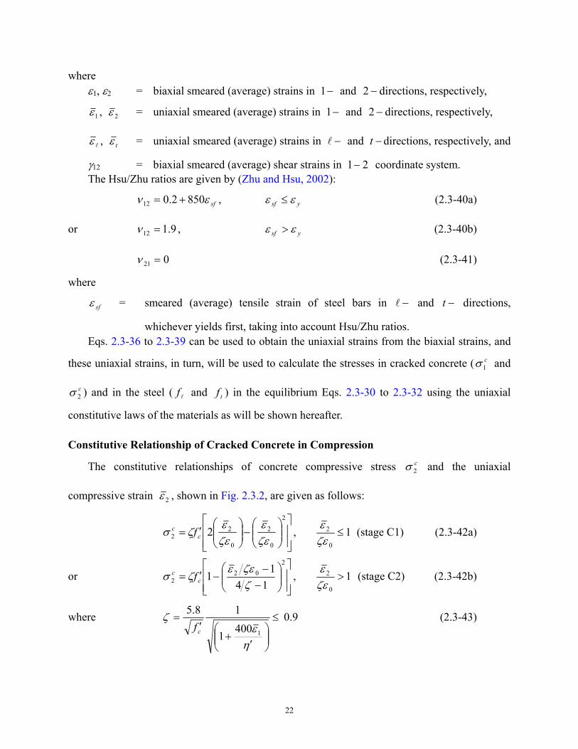
22

where ε1, ε2 = biaxial smeared (average) strains in −1 and −2 directions, respectively,

1ε , 2ε = uniaxial smeared (average) strains in −1 and −2 directions, respectively,

lε , tε = uniaxial smeared (average) strains in −l and −t directions, respectively, and

γ12 = biaxial smeared (average) shear strains in 21− coordinate system. The Hsu/Zhu ratios are given by (Zhu and Hsu, 2002):

sfεν 8502.012 += , ysf εε ≤ (2.3-40a)

or 9.112 =ν , ysf εε > (2.3-40b)

021 =ν (2.3-41)

where

sfε = smeared (average) tensile strain of steel bars in −l and −t directions,

whichever yields first, taking into account Hsu/Zhu ratios. Eqs. 2.3-36 to 2.3-39 can be used to obtain the uniaxial strains from the biaxial strains, and

these uniaxial strains, in turn, will be used to calculate the stresses in cracked concrete ( c1σ and

c2σ ) and in the steel ( lf and tf ) in the equilibrium Eqs. 2.3-30 to 2.3-32 using the uniaxial

constitutive laws of the materials as will be shown hereafter.

Constitutive Relationship of Cracked Concrete in Compression

The constitutive relationships of concrete compressive stress c2σ and the uniaxial

compressive strain 2ε , shown in Fig. 2.3.2, are given as follows:

−

′=

2

0

2

0

22 2

ζεε

ζεε

ζσ cc f , 1

0

2 ≤ζεε (stage C1) (2.3-42a)

or

−

−−′=

202

2 141

1ζζεε

ζσ cc f , 1

0

2 >ζεε (stage C2) (2.3-42b)

where 9.0 4001

18.5

1

≤

′

+′

=

ηε

ζcf

(2.3-43)

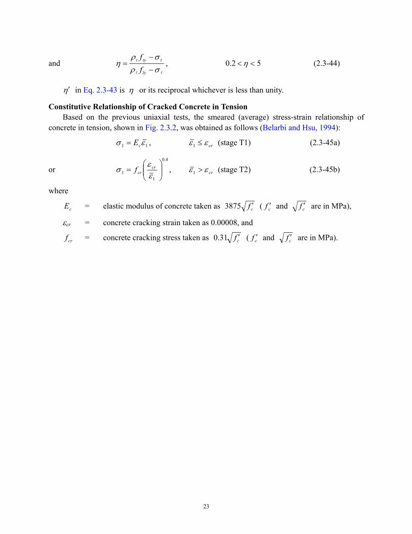
23

and ll σρ

σρη

−

−=

ly

ttyt

ff

, 52.0 << η (2.3-44)

η′ in Eq. 2.3-43 is η or its reciprocal whichever is less than unity.

Constitutive Relationship of Cracked Concrete in Tension Based on the previous uniaxial tests, the smeared (average) stress-strain relationship of

concrete in tension, shown in Fig. 2.3.2, was obtained as follows (Belarbi and Hsu, 1994):

11 εσ cE= , crεε ≤1 (stage T1) (2.3-45a)

or 4.0

11

=

εε

σ crcrf , crεε >1 (stage T2) (2.3-45b)

where




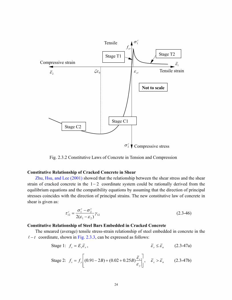
24

Constitutive Relationship of Cracked Concrete in Shear

Zhu, Hsu, and Lee (2001) showed that the relationship between the shear stress and the shear strain of cracked concrete in the 21− coordinate system could be rationally derived from the equilibrium equations and the compatibility equations by assuming that the direction of principal stresses coincides with the direction of principal strains. The new constitutive law of concrete in shear is given as:

1221

2112 )(2

γεεσσ

τ−−

=cc

c (2.3-46)

Constitutive Relationship of Steel Bars Embedded in Cracked Concrete The smeared (average) tensile stress-strain relationship of steel embedded in concrete in the

t−l coordinate, shown in Fig. 2.3.3, can be expressed as follows:

Stage 1: sss Ef ε= , ns εε ≤ (2.3-47a)

Stage 2:

++−=

y

sys BBff

εε

)25.002.0()291.0( , ns εε > (2.3-47b)

2ε

1ε

c2σ

c1σ

crf

crε0ζε

Stage C1Stage C2

Stage T2 Stage T1Compressive strain

Tensile strain

Compressive stress

Tensile

Not to scale

Fig. 2.3.2 Constitutive Laws of Concrete in Tension and Compression

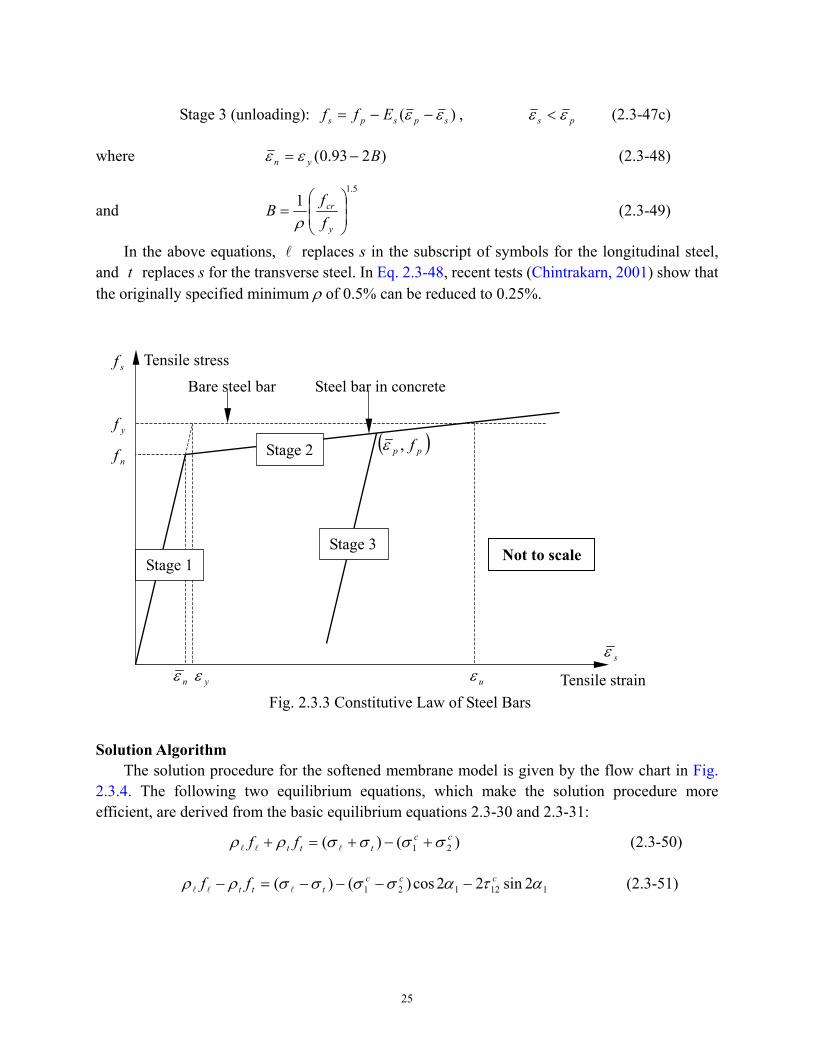
25

Stage 3 (unloading): )( spsps Eff εε −−= , ps εε < (2.3-47c)

where )293.0( Byn −= εε (2.3-48)

and 5.1

1

=

y

cr

ff

Bρ

(2.3-49)

In the above equations, l replaces s in the subscript of symbols for the longitudinal steel, and t replaces s for the transverse steel. In Eq. 2.3-48, recent tests (Chintrakarn, 2001) show that the originally specified minimum ρ of 0.5% can be reduced to 0.25%.

Solution Algorithm

The solution procedure for the softened membrane model is given by the flow chart in Fig. 2.3.4. The following two equilibrium equations, which make the solution procedure more efficient, are derived from the basic equilibrium equations 2.3-30 and 2.3-31:

)()( 21cc

ttt ff σσσσρρ +−+=+ lll (2.3-50)

112121 2sin22cos)()( ατασσσσρρ cccttt ff −−−−=− lll (2.3-51)

sf

sε

yf

nf

nε yε

( )pp f,ε

uε

Stage 1

Stage 2

Stage 3

Bare steel bar Steel bar in concrete

Tensile strain

Tensile stress

Not to scale

Fig. 2.3.3 Constitutive Law of Steel Bars

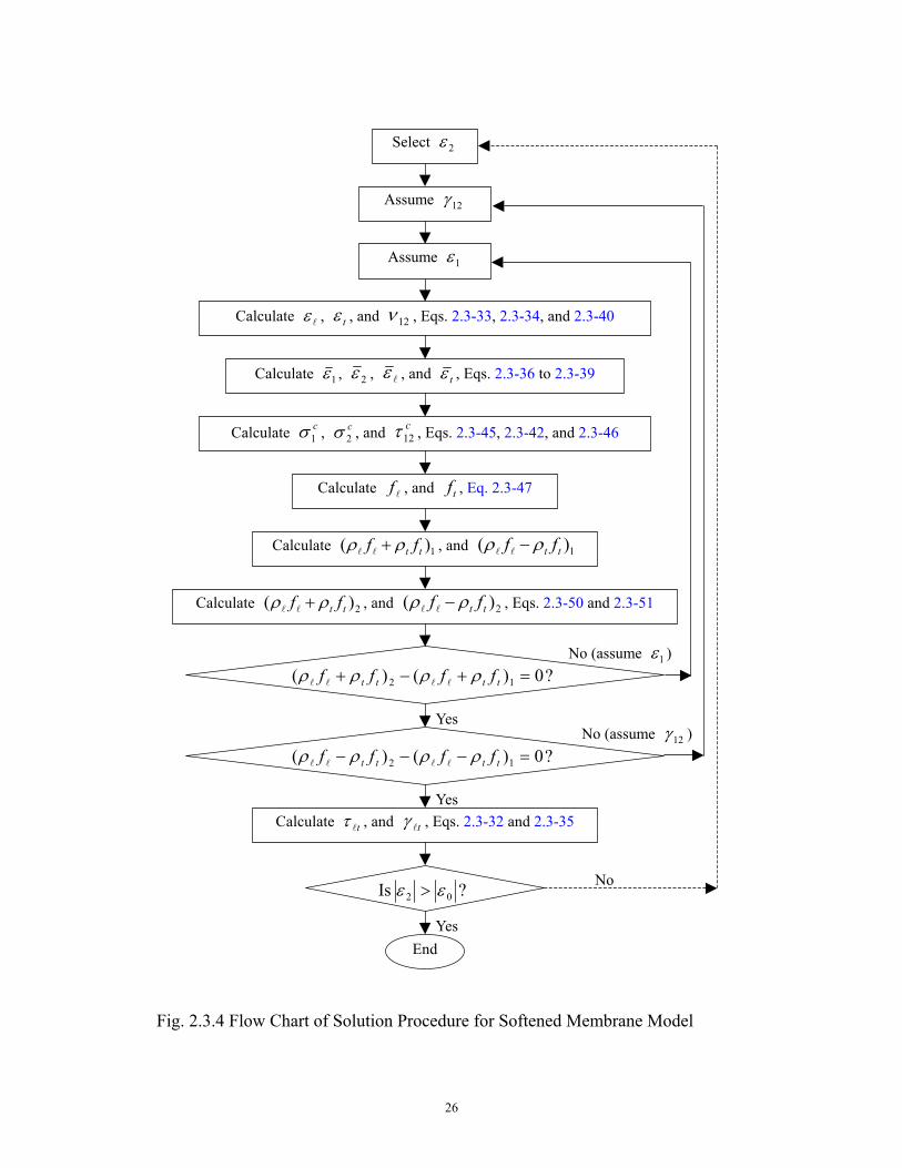
26

Select 2ε

Assume 12γ

Assume 1ε

Calculate lε , tε , and 12ν , Eqs. 2.3-33, 2.3-34, and 2.3-40

Calculate 1ε , 2ε , lε , and tε , Eqs. 2.3-36 to 2.3-39

Calculate c1σ , c

2σ , and c12τ , Eqs. 2.3-45, 2.3-42, and 2.3-46

Calculate lf , and tf , Eq. 2.3-47

Calculate 1)( tt ff ρρ +ll , and 1)( tt ff ρρ −ll

Calculate 2)( tt ff ρρ +ll , and 2)( tt ff ρρ −ll , Eqs. 2.3-50 and 2.3-51

?0)()( 12 =+−+ tttt ffff ρρρρ llll

?0)()( 12 =−−− tttt ffff ρρρρ llll

Calculate tlτ , and tlγ , Eqs. 2.3-32 and 2.3-35

? Is 02 εε >

End

No (assume 1ε )

No (assume 12γ )

No

Yes

Yes

Yes

Fig. 2.3.4 Flow Chart of Solution Procedure for Softened Membrane Model

27

2.4 Literature Survey on Shear Behavior of Prestressed Concrete Panels Very little experimental research has been done on the behavior of prestressed concrete

membrane elements (panels) under shear stresses. The main difficulties involved in performing these kinds of tests were the high cost of testing equipment and the complexity in fabricating prestressed concrete panels.

Marti and Meyboom (1992) discussed the influence of prestressing on the behavior of orthogonally reinforced concrete elements subjected to in-plane shear forces. Meyboom (1987) reported three tests performed on the University of Toronto’s shell element tester. All three specimens had identical dimensions of mm 287mm 1626mm 1626 ×× ( in. 11.3in. 64in. 64 ×× ). The only variable was the amount of prestressing in the 45-degree direction: Specimen PP1 was not prestressed, Specimen PP2 was prestressed to 2.07 MPa (301 psi), and Specimen PP3 was prestressed to 4.40 MPa (638 psi). Based on these test results, the authors concluded that prestressing results in higher cracking loads, reduced reorientation of the internal forces after cracking, delayed degradation of the concrete, smaller strains in the reinforcements at ultimate, and higher ultimate loads. The experimental responses were compared with the predicted responses made by linear, nonlinear, and limit analyses as given in the paper. However, there were several deficiencies in the study: First, they did not give the properties of materials in prestressed concrete panels, so only a qualitative analysis could be performed. The effect of prestressing on the constitutive laws of the concrete was not clarified. Second, since mild steel bars were oriented in the direction of the unbonded prestressing bars, the crack patterns were caused mainly by the distribution of the mild steel bars. Finally, the descending branches for the shear stress-strain curve could not be obtained because the tester was not equipped with a servo-controlled system.

Rahal (2002) proposed a method for the analysis and design of concrete membrane elements subjected to in-plane shear and normal stresses, which is a simplification of the modified compression field theory (Vecchio and Collins, 1986). In this method, a prestress force was simply considered as a superimposed normal stress on the panels. The experimental results of Meyboom (1987) were used to check his method. It was concluded that a significant increase of prestressing stresses produced only a slight increase in shear strength. Also, the effect of prestressing on the shear behavior of the prestressed concrete elements could not be verified due to the limitation of experimental results.

29

CHAPTER 3

CRACK SIMULATION TESTS

3.1 General Description Prestressed concrete is classified into “pre-tensioned concrete” and “post-tensioned

concrete” by the sequence of concrete placement and tensioning of high-strength steel. Pre-tensioning technology is more commonly used than post-tensioning in highway bridges, because it is more convenient for mass production. According to ACI 318-02 Eq. 12-2, the transfer length in concrete pre-tensioned by 270K ( MPa 1862 ) strands with an assumed effective stress of

MPa 965 ( ksi 140 ) is 50 times the strand diameter, giving mm 750 ( in. 30 ) and mm 625 ( in. 25 ) for diameters of in. 0.6 ( mm 15 ) and in. 0.5 ( mm 13 ) strands, respectively. The corresponding development lengths in pre-tensioned concrete are mm 2692 ( in. 106 ) and

mm 2235 ( in. 88 ), respectively. Since these transfer lengths and development lengths are too large for the test panels of mm 1398mm 1398 × ( in. 55in. 55 × ), the post-tensioning method was chosen for the test panels in this research. The post-tensioned strands were placed in flexible conduits and then grouted.

A trial panel, labeled TE-2, was first tested. The arrangement of the reinforcements of panel TE-2 is shown in Fig. 3.1.1. Prestressing tendons were placed in the longitudinal direction and the post-tensioning technology was used. This panel was tested under applied tensile forces in the longitudinal direction. The crack pattern of panel TE-2 at 2% tensile strain is shown in Fig. 3.1.2. The crack spacing, approximately mm 610 ( in. 24 ), was excessive due to the weak bond between the prestressing tendons and the cementitious grout. The smeared-crack concept as an average quantity of strain could not be applied in this case with only two big cracks occurring in the measurement zone. Therefore, a series of crack simulation tests was performed to improve the bond condition between the steel tendons and the cementitious grout. The purpose of the study was to find the same cracking pattern of post-tensioned concrete with conduits as that in pre-tensioned concrete without conduits.

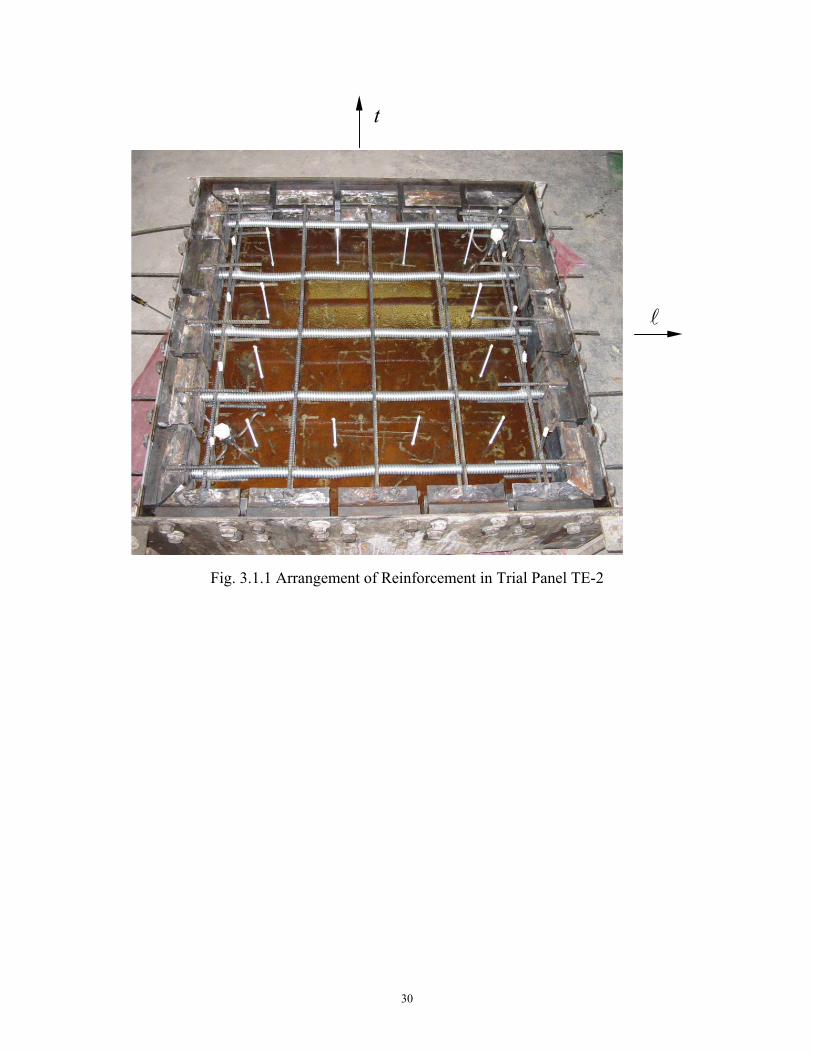
30

Fig. 3.1.1 Arrangement of Reinforcement in Trial Panel TE-2

l

t

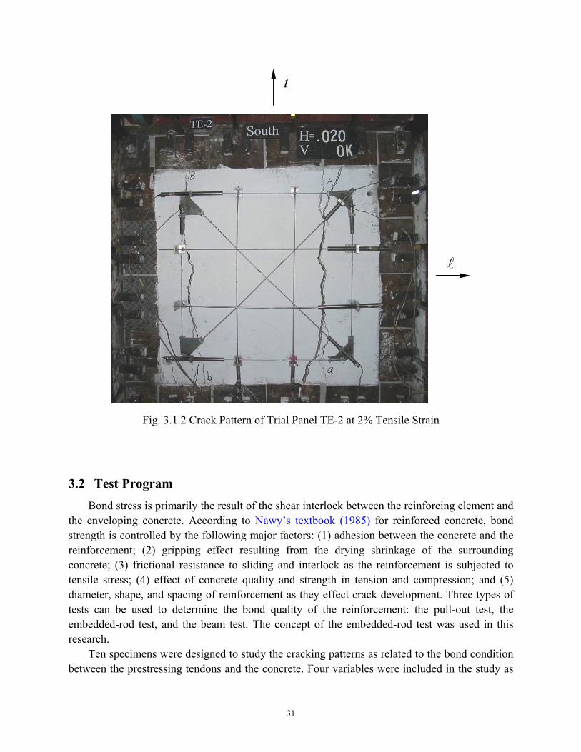
31

3.2 Test Program Bond stress is primarily the result of the shear interlock between the reinforcing element and

the enveloping concrete. According to Nawy’s textbook (1985) for reinforced concrete, bond strength is controlled by the following major factors: (1) adhesion between the concrete and the reinforcement; (2) gripping effect resulting from the drying shrinkage of the surrounding concrete; (3) frictional resistance to sliding and interlock as the reinforcement is subjected to tensile stress; (4) effect of concrete quality and strength in tension and compression; and (5) diameter, shape, and spacing of reinforcement as they effect crack development. Three types of tests can be used to determine the bond quality of the reinforcement: the pull-out test, the embedded-rod test, and the beam test. The concept of the embedded-rod test was used in this research.

Ten specimens were designed to study the cracking patterns as related to the bond condition between the prestressing tendons and the concrete. Four variables were included in the study as

Fig. 3.1.2 Crack Pattern of Trial Panel TE-2 at 2% Tensile Strain

l

t

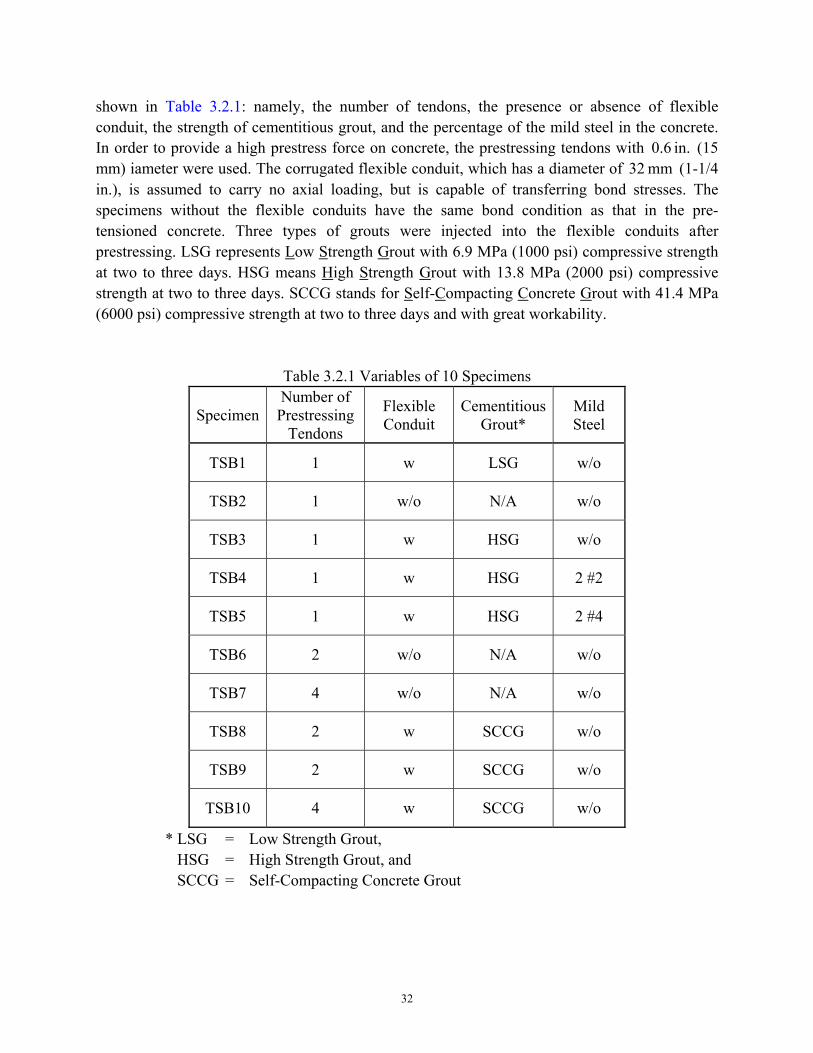
32

shown in Table 3.2.1: namely, the number of tendons, the presence or absence of flexible conduit, the strength of cementitious grout, and the percentage of the mild steel in the concrete. In order to provide a high prestress force on concrete, the prestressing tendons with in. 0.6 (15 mm) iameter were used. The corrugated flexible conduit, which has a diameter of mm 32 (1-1/4 in.), is assumed to carry no axial loading, but is capable of transferring bond stresses. The specimens without the flexible conduits have the same bond condition as that in the pre-tensioned concrete. Three types of grouts were injected into the flexible conduits after prestressing. LSG represents Low Strength Grout with 6.9 MPa (1000 psi) compressive strength at two to three days. HSG means High Strength Grout with 13.8 MPa (2000 psi) compressive strength at two to three days. SCCG stands for Self-Compacting Concrete Grout with 41.4 MPa (6000 psi) compressive strength at two to three days and with great workability.

Table 3.2.1 Variables of 10 Specimens

Specimen Number of Prestressing

Tendons

Flexible Conduit

Cementitious Grout*

Mild Steel

TSB1 1 w LSG w/o

TSB2 1 w/o N/A w/o

TSB3 1 w HSG w/o

TSB4 1 w HSG 2 #2

TSB5 1 w HSG 2 #4

TSB6 2 w/o N/A w/o

TSB7 4 w/o N/A w/o

TSB8 2 w SCCG w/o

TSB9 2 w SCCG w/o

TSB10 4 w SCCG w/o

* LSG = Low Strength Grout, HSG = High Strength Grout, and SCCG = Self-Compacting Concrete Grout

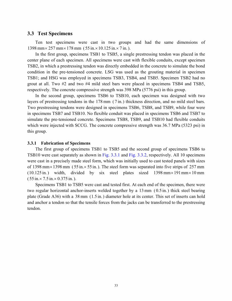
33

3.3 Test Specimens Ten test specimens were cast in two groups and had the same dimensions of

mm 178mm 257mm 1398 ×× ( in. 7in. 10.125in. 55 ×× ). In the first group, specimens TSB1 to TSB5, a single prestressing tendon was placed in the

center plane of each specimen. All specimens were cast with flexible conduits, except specimen TSB2, in which a prestressing tendon was directly embedded in the concrete to simulate the bond condition in the pre-tensioned concrete. LSG was used as the grouting material in specimen TSB1; and HSG was employed in specimens TSB3, TSB4, and TSB5. Specimen TSB2 had no grout at all. Two #2 and two #4 mild steel bars were placed in specimens TSB4 and TSB5, respectively. The concrete compressive strength was 398 MPa (5776 psi) in this group.

In the second group, specimens TSB6 to TSB10, each specimen was designed with two layers of prestressing tendons in the mm 178 ( in. 7 ) thickness direction, and no mild steel bars. Two prestressing tendons were designed in specimens TSB6, TSB8, and TSB9, while four were in specimens TSB7 and TSB10. No flexible conduit was placed in specimens TSB6 and TSB7 to simulate the pre-tensioned concrete. Specimens TSB8, TSB9, and TSB10 had flexible conduits which were injected with SCCG. The concrete compressive strength was 36.7 MPa (5323 psi) in this group.

3.3.1 Fabrication of Specimens

The first group of specimens TSB1 to TSB5 and the second group of specimens TSB6 to TSB10 were cast separately as shown in Fig. 3.3.1 and Fig. 3.3.2, respectively. All 10 specimens were cast in a precisely made steel form, which was initially used to cast tested panels with sizes of mm 1398mm 1398 × ( in. 55in. 55 × ). The steel form was separated into five strips of mm 257 ( in. 10.125 ) width, divided by six steel plates sized mm 10mm 191mm 1398 ×× ( in. 0.375in. 7.5in. 55 ×× ).

Specimens TSB1 to TSB5 were cast and tested first. At each end of the specimen, there were two regular horizontal anchor-inserts welded together by a mm 13 ( in. 0.5 ) thick steel bearing plate (Grade A36) with a mm 38 ( in. 1.5 ) diameter hole at its center. This set of inserts can hold and anchor a tendon so that the tensile forces from the jacks can be transferred to the prestressing tendon.

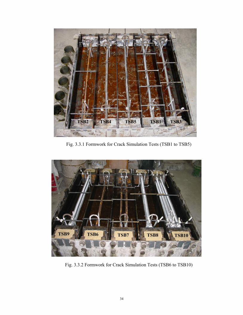
34

TSB9 TSB6 TSB7 TSB8 TSB10

Fig. 3.3.1 Formwork for Crack Simulation Tests (TSB1 to TSB5)

TSB2 TSB4 TSB5 TSB1 TSB3



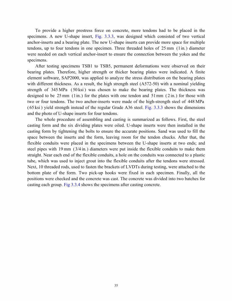
35

To provide a higher prestress force on concrete, more tendons had to be placed in the specimens. A new U-shape insert, Fig. 3.3.3, was designed which consisted of two vertical anchor-inserts and a bearing plate. The new U-shape inserts can provide more space for multiple tendons, up to four tendons in one specimen. Three threaded holes of mm 25 ( in. 1 ) diameter were needed on each vertical anchor-insert to ensure the connection between the yokes and the specimens.

After testing specimens TSB1 to TSB5, permanent deformations were observed on their bearing plates. Therefore, higher strength or thicker bearing plates were indicated. A finite element software, SAP2000, was applied to analyze the stress distribution on the bearing plates with different thickness. As a result, the high strength steel (A572-50) with a nominal yielding strength of MPa 345 ( ksi 50 ) was chosen to make the bearing plates. The thickness was designed to be mm 25 ( in. 1 ) for the plates with one tendon and mm 51 ( in. 2 ) for those with two or four tendons. The two anchor-inserts were made of the high-strength steel of MPa 448 ( ksi 65 ) yield strength instead of the regular Grade A36 steel. Fig. 3.3.3 shows the dimensions and the photo of U-shape inserts for four tendons.

The whole procedure of assembling and casting is summarized as follows. First, the steel casting form and the six dividing plates were oiled. U-shape inserts were then installed in the casting form by tightening the bolts to ensure the accurate positions. Sand was used to fill the space between the inserts and the form, leaving room for the tendon chucks. After that, the flexible conduits were placed in the specimens between the U-shape inserts at two ends; and steel pipes with mm 19 ( in. 3/4 ) diameters were put inside the flexible conduits to make them straight. Near each end of the flexible conduits, a hole on the conduits was connected to a plastic tube, which was used to inject grout into the flexible conduits after the tendons were stressed. Next, 10 threaded rods, used to fasten the brackets of LVDTs during testing, were attached to the bottom plate of the form. Two pick-up hooks were fixed in each specimen. Finally, all the positions were checked and the concrete was cast. The concrete was divided into two batches for casting each group. Fig 3.3.4 shows the specimens after casting concrete.

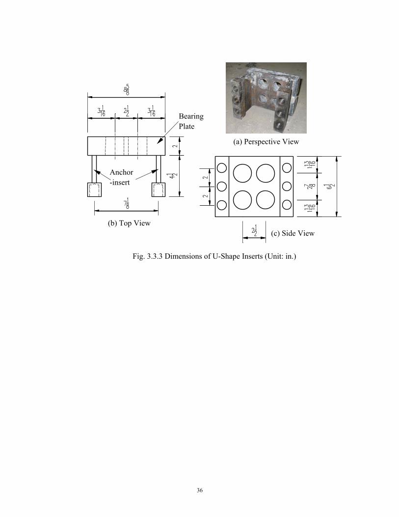
36

Fig. 3.3.3 Dimensions of U-Shape Inserts (Unit: in.)

(a) Perspective View

(b) Top View (c) Side View

Bearing Plate

Anchor-insert

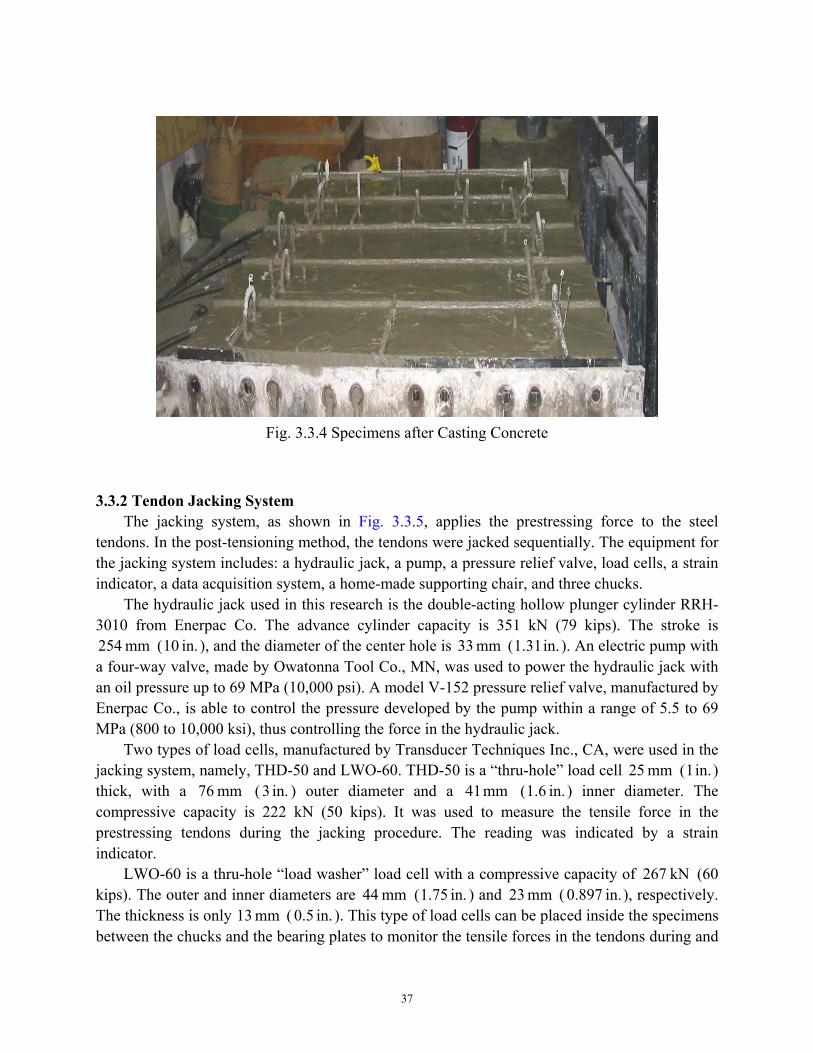
37

3.3.2 Tendon Jacking System

The jacking system, as shown in Fig. 3.3.5, applies the prestressing force to the steel tendons. In the post-tensioning method, the tendons were jacked sequentially. The equipment for the jacking system includes: a hydraulic jack, a pump, a pressure relief valve, load cells, a strain indicator, a data acquisition system, a home-made supporting chair, and three chucks.

The hydraulic jack used in this research is the double-acting hollow plunger cylinder RRH-3010 from Enerpac Co. The advance cylinder capacity is 351 kN (79 kips). The stroke is

mm 254 ( in. 10 ), and the diameter of the center hole is mm 33 ( in. 1.31 ). An electric pump with a four-way valve, made by Owatonna Tool Co., MN, was used to power the hydraulic jack with an oil pressure up to 69 MPa (10,000 psi). A model V-152 pressure relief valve, manufactured by Enerpac Co., is able to control the pressure developed by the pump within a range of 5.5 to 69 MPa (800 to 10,000 ksi), thus controlling the force in the hydraulic jack.

Two types of load cells, manufactured by Transducer Techniques Inc., CA, were used in the jacking system, namely, THD-50 and LWO-60. THD-50 is a “thru-hole” load cell mm 25 ( in. 1 ) thick, with a mm 76 ( in. 3 ) outer diameter and a mm41 ( in. 1.6 ) inner diameter. The compressive capacity is 222 kN (50 kips). It was used to measure the tensile force in the prestressing tendons during the jacking procedure. The reading was indicated by a strain indicator.

LWO-60 is a thru-hole “load washer” load cell with a compressive capacity of kN 267 (60 kips). The outer and inner diameters are mm44 ( in. 1.75 ) and mm 23 ( in. 0.897 ), respectively. The thickness is only mm 13 ( in. 0.5 ). This type of load cells can be placed inside the specimens between the chucks and the bearing plates to monitor the tensile forces in the tendons during and

Fig. 3.3.4 Specimens after Casting Concrete

38

after prestressing. A data acquisition system called Spider 8 was used to collect the readings from all the LWO-60 load cells.

The supporting chair consists of two 25 mm (1 in.) thick steel plates, four threaded bolts, and eight nuts. The chair is designed to transfer the force of the hydraulic jack to the test specimen. The height of the chair is adjustable.

Fig. 3.3.5(a) is a sketch of the tendon jacking system. Three chucks are used in the jacking system. The first chuck on the left end, which is next to a load cell LWO-60, grips one end of the tendon. On the right end, the second chuck holds the tendon against the hydraulic jack. Load cell THD-50 is placed between this chuck and the jack piston (Fig. 3.3.5(c)). The jack sits on the supporting chair against the specimen. The third chuck is located in the space enclosed by U-shape inserts. This chuck is kept loose during the jacking process, but catches the tendon once the releasing procedure starts. After all the setup was ready, the pump would be turned on to increase the pressure in the jack. The whole jacking procedure was summarized into five steps. First, a small force was applied to tighten the setup, and the positions of all the components were checked. Second, the tendon was pulled until the desired tensile force was reached. The pulling stage was divided into about 15 steps. At each step, the readings from load cells THD-50 and LWO-60 were recorded. Because the thickness of LWO-60 was very small, the reading was very sensitive to the eccentricity of the load (did not happen on THD-50). Therefore, the data from THD-50 would be used to calibrate the LWO-60 load cells.

In the third step, the nut bearing against the right plate of the supporting chair was turned to push and tighten the chuck against the test specimen, as shown in Fig. 3.3.5(b). This is one of the two methods to reduce the prestress loss due to the anchorage slippage. The other method is to utilize the pressure relief valve. Fourth, the pressure relief valve was turned to slowly release the pressure in the hydraulic jack. By applying those two methods, the prestress loss could be minimized. These two methods not only reduced the prestress loss, but also stabilized the loss, which could make the forces in the tendons more uniform in the test panel. The data showed that the effective stress in in. 0.6 tendons was approximately MPa 965 ( ksi 140 ) with a jacking stress of MPa 1303 ( ksi 189 ). Upon release, the middle chuck served to catch the tendon. Finally, all equipment was removed from the specimen and the redundant parts of the tendons were cut off.

In addition to slippage and elastic loss, prestress losses also include time-related losses, such as creep and shrinkage in the concrete and relaxation in the steel. To limit these time-dependent losses and to keep the high prestressed forces on the specimens, tests were conducted as soon as possible after the tensioning procedure. Experience shows that two to three days would be needed to inject grout into the flexible conduits, to install yokes, to put specimens in the Univers-

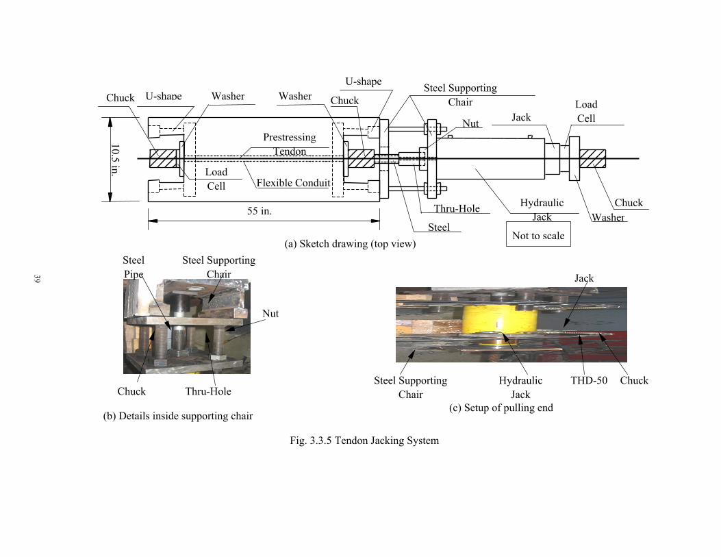
39

Fig. 3.3.5 Tendon Jacking System

Washer Washer Chuck

Chuck

Chuck

Load Cell

Load Cell

Steel Supporting Chair

Hydraulic Jack 55 in.

10.5in.

Thru-Hole

Steel

Flexible Conduit

Prestressing Tendon

Nut

Not to scale


Thru-Hole

Steel Pipe

Nut

Chuck

Washer

Chuck THD-50 Hydraulic Jack


(a) Sketch drawing (top view)

(b) Details inside supporting chair (c) Setup of pulling end

Jack

U-shape U-shape

Jack

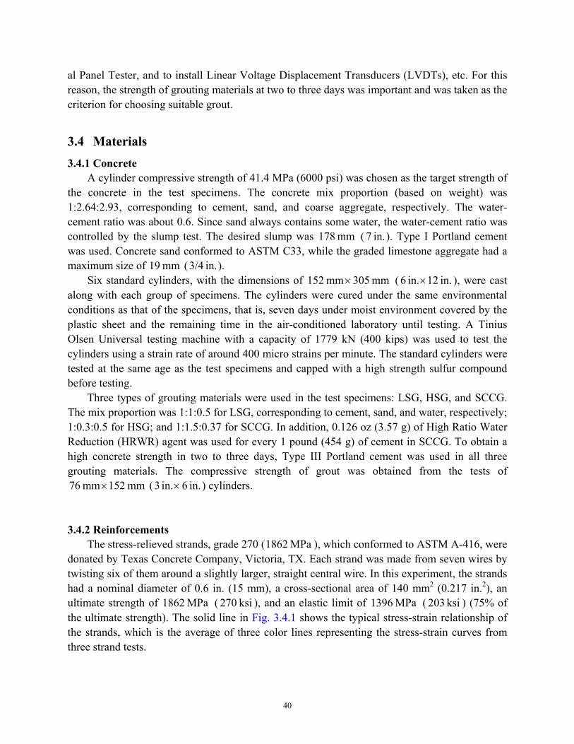
40

al Panel Tester, and to install Linear Voltage Displacement Transducers (LVDTs), etc. For this reason, the strength of grouting materials at two to three days was important and was taken as the criterion for choosing suitable grout.

3.4 Materials 3.4.1 Concrete

A cylinder compressive strength of 41.4 MPa (6000 psi) was chosen as the target strength of the concrete in the test specimens. The concrete mix proportion (based on weight) was 1:2.64:2.93, corresponding to cement, sand, and coarse aggregate, respectively. The water-cement ratio was about 0.6. Since sand always contains some water, the water-cement ratio was controlled by the slump test. The desired slump was mm 178 ( in. 7 ). Type I Portland cement was used. Concrete sand conformed to ASTM C33, while the graded limestone aggregate had a maximum size of mm 19 ( in. 3/4 ).

Six standard cylinders, with the dimensions of mm 305mm 152 × ( in. 12in. 6 × ), were cast along with each group of specimens. The cylinders were cured under the same environmental conditions as that of the specimens, that is, seven days under moist environment covered by the plastic sheet and the remaining time in the air-conditioned laboratory until testing. A Tinius Olsen Universal testing machine with a capacity of 1779 kN (400 kips) was used to test the cylinders using a strain rate of around 400 micro strains per minute. The standard cylinders were tested at the same age as the test specimens and capped with a high strength sulfur compound before testing.

Three types of grouting materials were used in the test specimens: LSG, HSG, and SCCG. The mix proportion was 1:1:0.5 for LSG, corresponding to cement, sand, and water, respectively; 1:0.3:0.5 for HSG; and 1:1.5:0.37 for SCCG. In addition, 0.126 oz (3.57 g) of High Ratio Water Reduction (HRWR) agent was used for every 1 pound (454 g) of cement in SCCG. To obtain a high concrete strength in two to three days, Type III Portland cement was used in all three grouting materials. The compressive strength of grout was obtained from the tests of

mm 152mm 76 × ( in. 6in. 3 × ) cylinders.

3.4.2 Reinforcements The stress-relieved strands, grade 270 ( MPa 1862 ), which conformed to ASTM A-416, were

donated by Texas Concrete Company, Victoria, TX. Each strand was made from seven wires by twisting six of them around a slightly larger, straight central wire. In this experiment, the strands had a nominal diameter of 0.6 in. (15 mm), a cross-sectional area of 140 mm2 (0.217 in.2), an ultimate strength of MPa 1862 ( ksi 270 ), and an elastic limit of MPa 1396 ( ksi 203 ) (75% of the ultimate strength). The solid line in Fig. 3.4.1 shows the typical stress-strain relationship of the strands, which is the average of three color lines representing the stress-strain curves from three strand tests.

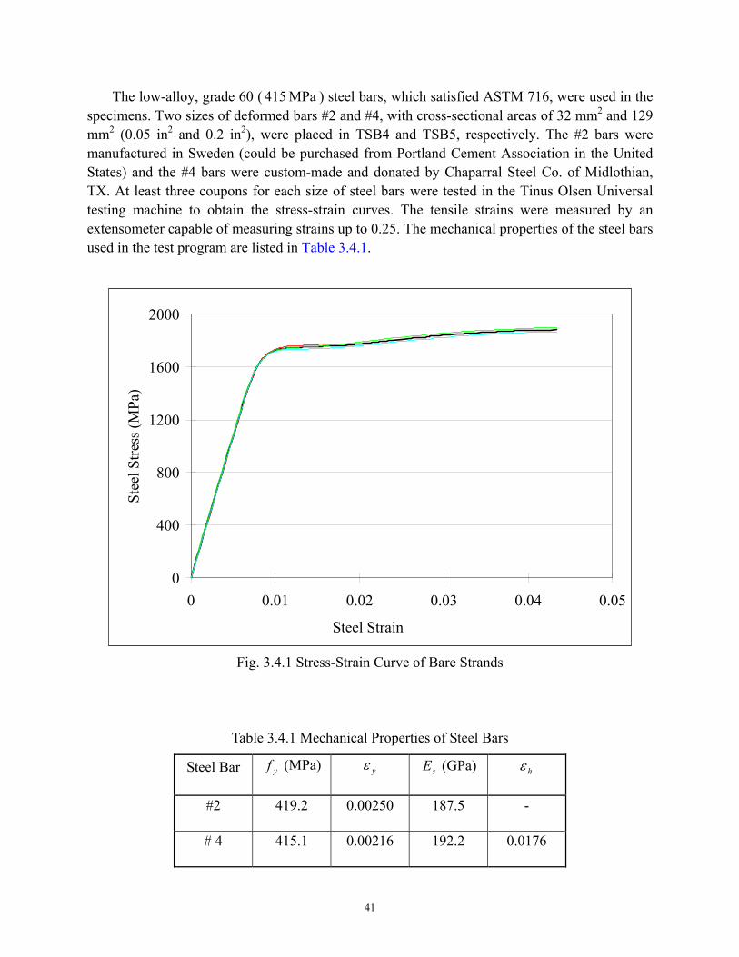
41

The low-alloy, grade 60 ( MPa 415 ) steel bars, which satisfied ASTM 716, were used in the specimens. Two sizes of deformed bars #2 and #4, with cross-sectional areas of 32 mm2 and 129 mm2 (0.05 in2 and 0.2 in2), were placed in TSB4 and TSB5, respectively. The #2 bars were manufactured in Sweden (could be purchased from Portland Cement Association in the United States) and the #4 bars were custom-made and donated by Chaparral Steel Co. of Midlothian, TX. At least three coupons for each size of steel bars were tested in the Tinus Olsen Universal testing machine to obtain the stress-strain curves. The tensile strains were measured by an extensometer capable of measuring strains up to 0.25. The mechanical properties of the steel bars used in the test program are listed in Table 3.4.1.

Table 3.4.1 Mechanical Properties of Steel Bars

Steel Bar yf (MPa) yε sE (GPa) hε

#2 419.2 0.00250 187.5 -

# 4 415.1 0.00216 192.2 0.0176

Fig. 3.4.1 Stress-Strain Curve of Bare Strands

0

400

800

1200

1600

2000

0 0.01 0.02 0.03 0.04 0.05

Steel Strain

Stee

l Stre

ss (M

Pa)

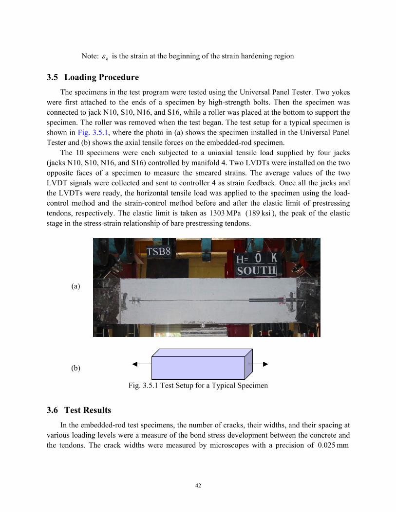
42

Note: hε is the strain at the beginning of the strain hardening region

3.5 Loading Procedure The specimens in the test program were tested using the Universal Panel Tester. Two yokes

were first attached to the ends of a specimen by high-strength bolts. Then the specimen was connected to jack N10, S10, N16, and S16, while a roller was placed at the bottom to support the specimen. The roller was removed when the test began. The test setup for a typical specimen is shown in Fig. 3.5.1, where the photo in (a) shows the specimen installed in the Universal Panel Tester and (b) shows the axial tensile forces on the embedded-rod specimen.

The 10 specimens were each subjected to a uniaxial tensile load supplied by four jacks (jacks N10, S10, N16, and S16) controlled by manifold 4. Two LVDTs were installed on the two opposite faces of a specimen to measure the smeared strains. The average values of the two LVDT signals were collected and sent to controller 4 as strain feedback. Once all the jacks and the LVDTs were ready, the horizontal tensile load was applied to the specimen using the load-control method and the strain-control method before and after the elastic limit of prestressing tendons, respectively. The elastic limit is taken as MPa 1303 ( ksi 189 ), the peak of the elastic stage in the stress-strain relationship of bare prestressing tendons.

3.6 Test Results In the embedded-rod test specimens, the number of cracks, their widths, and their spacing at

various loading levels were a measure of the bond stress development between the concrete and the tendons. The crack widths were measured by microscopes with a precision of mm 0.025

Fig. 3.5.1 Test Setup for a Typical Specimen

(a)

(b)

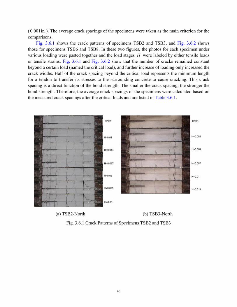
43

( in. 0.001 ). The average crack spacings of the specimens were taken as the main criterion for the comparisons.

Fig. 3.6.1 shows the crack patterns of specimens TSB2 and TSB3, and Fig. 3.6.2 shows those for specimens TSB6 and TSB8. In these two figures, the photos for each specimen under various loading were pasted together and the load stages H were labeled by either tensile loads or tensile strains. Fig. 3.6.1 and Fig. 3.6.2 show that the number of cracks remained constant beyond a certain load (named the critical load), and further increase of loading only increased the crack widths. Half of the crack spacing beyond the critical load represents the minimum length for a tendon to transfer its stresses to the surrounding concrete to cause cracking. This crack spacing is a direct function of the bond strength. The smaller the crack spacing, the stronger the bond strength. Therefore, the average crack spacings of the specimens were calculated based on the measured crack spacings after the critical loads and are listed in Table 3.6.1.

Fig. 3.6.1 Crack Patterns of Specimens TSB2 and TSB3

(a) TSB2-North (b) TSB3-North

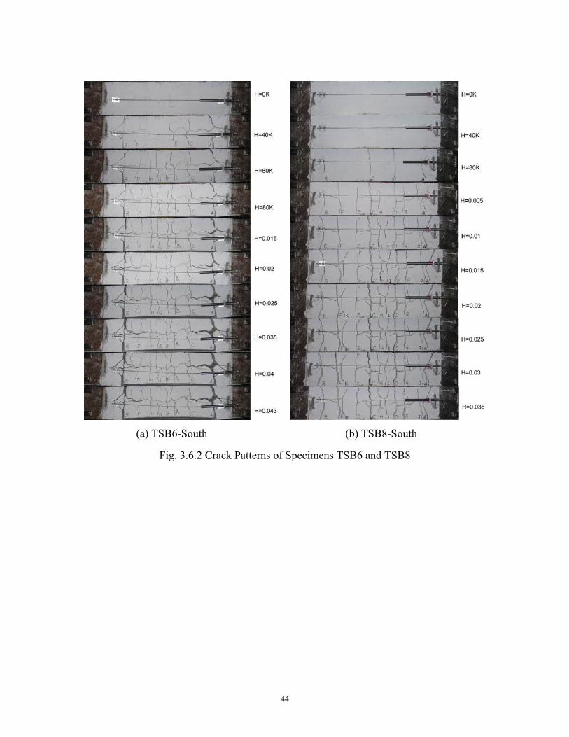
44

Fig. 3.6.2 Crack Patterns of Specimens TSB6 and TSB8

(a) TSB6-South (b) TSB8-South

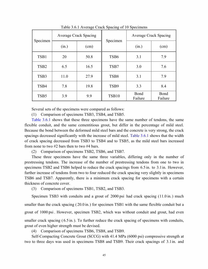
45

Table 3.6.1 Average Crack Spacing of 10 Specimens

Average Crack Spacing Average Crack Spacing Specimen

(in.) (cm) Specimen

(in.) (cm)

TSB1 20 50.8 TSB6 3.1 7.9

TSB2 6.5 16.5 TSB7 3.0 7.6

TSB3 11.0 27.9 TSB8 3.1 7.9

TSB4 7.8 19.8 TSB9 3.3 8.4

TSB5 3.9 9.9 TSB10 Bond Failure

Bond Failure

Several sets of the specimens were compared as follows: (1) Comparison of specimens TSB3, TSB4, and TSB5. Table 3.6.1 shows that these three specimens have the same number of tendons, the same

flexible conduit, and the same cementitious grout, but differ in the percentage of mild steel. Because the bond between the deformed mild steel bars and the concrete is very strong, the crack spacings decreased significantly with the increase of mild steel. Table 3.6.1 shows that the width of crack spacing decreased from TSB3 to TSB4 and to TSB5, as the mild steel bars increased from none to two #2 bars then to two #4 bars.

(2) Comparison of specimens TSB2, TSB6, and TSB7. These three specimens have the same three variables, differing only in the number of

prestressing tendons. The increase of the number of prestressing tendons from one to two in specimens TSB2 and TSB6 helped to reduce the crack spacings from in. 6.5 to in. 3.1 However, further increase of tendons from two to four reduced the crack spacing very slightly in specimens TSB6 and TSB7. Apparently, there is a minimum crack spacing for specimens with a certain thickness of concrete cover.

(3) Comparison of specimens TSB1, TSB2, and TSB3.

Specimen TSB3 with conduits and a grout of psi 2000 had crack spacing ( in. 11.0 ) much

smaller than the crack spacing ( in. 20.0 ) for specimen TSB1 with the same flexible conduit but a

grout of psi 1000 . However, specimen TSB2, which was without conduit and grout, had even

smaller crack spacing ( in. 6.5 ). To further reduce the crack spacing of specimens with conduits, grout of even higher strength must be devised.

(4) Comparison of specimens TSB6, TSB8, and TSB9. Self-Compacting Concrete Grout (SCCG) with 41.4 MPa (6000 psi) compressive strength at

two to three days was used in specimens TSB8 and TSB9. Their crack spacings of in. 3.1 and

46

in. 3.3 , respectively, were essentially the same as the in. 3.1 spacing for specimen TSB6 devoid of conduit and grout. In other words, post-tensioned specimens with flexible conduits and SCC grout of 41.4 MPa (6000 psi) (TSB8 and TSB9) can be used to simulate the bond condition in the pre-tensioned specimen (TSB6).

3.7 Conclusions According to the test results of 10 embedded-rod specimens, it can be concluded that (1) the

bond condition in pre-tensioned concrete can be simulated by post-tensioned concrete with flexible conduits and SCC grout of 41.4 MPa (6000 psi); (2) the new U-shape insert was proven to be capable of carrying up to four prestressing tendons; and (3) the jacking system was successful in applying and controlling the prestress forces on the concrete. All these proven technologies will be applicable to test panels described in Chapters 4 and 5.

47

CHAPTER 4

PRESTRESSED CONCRETE 0-DEGREE PANELS UNDER

SEQUENTIAL LOADING

To establish a rational model for the action of shear on prestressed concrete, a total of 10

membrane elements (panels) were tested in this research. The panels were divided into two groups: TE and TA, according to the angle of steel bar orientation α1 with respect to the applied principal stresses. The α1 angles of groups TE and TA are 0o and 45o respectively. Panels with α1 = 0o are subjected to sequential loading to study the constitutive relationships of materials (concrete and prestressing tendons). Panels with α1 = 45o are subjected to pure shear (a special case of proportional loading) to study the shear behavior of prestressed concrete membrane elements. The test program and testing results of the five panels in Group TE are described and discussed in this chapter, while those of the five panels in Group TA are presented in Chapter 5.

4.1 Test Program (Group TE) The purpose of testing the five panels in Group TE is to obtain the constitutive laws of

concrete and steel tendons in prestressed concrete membrane elements. The five panels were

designed with two variables: (1) percentage of prestressing tendons plρ in the panels and (2)

tensile strain in the horizontal direction 1ε , which was maintained constant during the second

stage of the loading (see Section 4.4) in each panel. The two variables of Group TE are listed in Table 4.1.1.

The labels of all five specimens in Group TE start with the letter “T”, which signifies that these panels are reinforced with prestressing Tendons. The second letter “E” means that the steel grid was set parallel to the applied principal stresses, resulting in α1 = 0o.

All the panels were subjected to sequential loading. Tensile forces were first applied in the horizontal direction. After attaining the desired smeared (average) tensile strain in the panels, compressive stresses were gradually applied in the vertical direction until failure. During the first stage of the tensile loading, the constitutive laws of concrete in tension and prestressing tendons embedded in concrete were obtained. In the second stage of the compressive loading, the stress-strain relationships of concrete in compression were recorded, from which the experimental softening coefficients were obtained.

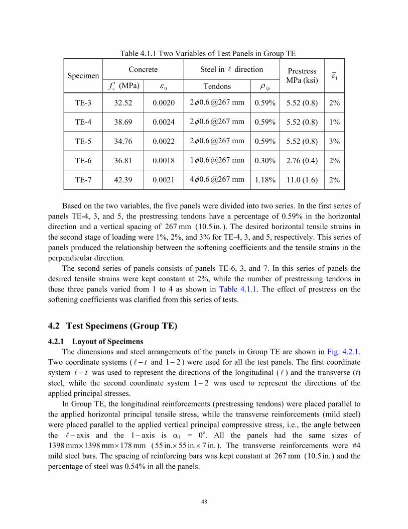
48

Table 4.1.1 Two Variables of Test Panels in Group TE

Concrete Steel in l direction Specimen

cf ′ (MPa) 0ε Tendons plρ

Prestress MPa (ksi) 1ε

TE-3 32.52 0.0020 2 6.0φ @267 mm 0.59% 5.52 (0.8) 2%

TE-4 38.69 0.0024 2 6.0φ @267 mm 0.59% 5.52 (0.8) 1%

TE-5 34.76 0.0022 2 6.0φ @267 mm 0.59% 5.52 (0.8) 3%

TE-6 36.81 0.0018 1 6.0φ @267 mm 0.30% 2.76 (0.4) 2%

TE-7 42.39 0.0021 4 6.0φ @267 mm 1.18% 11.0 (1.6) 2%

Based on the two variables, the five panels were divided into two series. In the first series of

panels TE-4, 3, and 5, the prestressing tendons have a percentage of 0.59% in the horizontal direction and a vertical spacing of mm 267 ( in. 10.5 ). The desired horizontal tensile strains in the second stage of loading were 1%, 2%, and 3% for TE-4, 3, and 5, respectively. This series of panels produced the relationship between the softening coefficients and the tensile strains in the perpendicular direction.

The second series of panels consists of panels TE-6, 3, and 7. In this series of panels the desired tensile strains were kept constant at 2%, while the number of prestressing tendons in these three panels varied from 1 to 4 as shown in Table 4.1.1. The effect of prestress on the softening coefficients was clarified from this series of tests.

4.2 Test Specimens (Group TE) 4.2.1 Layout of Specimens

The dimensions and steel arrangements of the panels in Group TE are shown in Fig. 4.2.1. Two coordinate systems ( t−l and 21− ) were used for all the test panels. The first coordinate system t−l was used to represent the directions of the longitudinal ( l ) and the transverse (t) steel, while the second coordinate system 21− was used to represent the directions of the applied principal stresses.

In Group TE, the longitudinal reinforcements (prestressing tendons) were placed parallel to the applied horizontal principal tensile stress, while the transverse reinforcements (mild steel) were placed parallel to the applied vertical principal compressive stress, i.e., the angle between the −l axis and the −1 axis is α1 = 0o. All the panels had the same sizes of

mm 178mm 1398mm 1398 ×× ( in. 7in. 55in. 55 ×× ). The transverse reinforcements were #4 mild steel bars. The spacing of reinforcing bars was kept constant at mm 267 ( in. 10.5 ) and the percentage of steel was 0.54% in all the panels.

49

The arrangement of the reinforcements in panels TE-4, 3, and 5 was identical as shown in Fig. 4.2.1(a). Five prestressing tendons (in the form of pairs) were placed in the horizontal direction in two layers. The center-to-center spacing between the two layers of tendons was 73 mm (2.88 in). The prestress force in each tendon was about 138 kN (31 kips), resulting in the prestress on the concrete of about MPa 5.52 ( ksi 0.8 ). Fig. 4.2.1(b) shows the steel grid of panel TE-6, which had only one layer of prestressing tendons. Five tendons with the spacing of

mm 267 ( in. 10.5 ) provided about MPa 2.76 ( ksi 0.4 ) prestress on the concrete. In Fig. 4.2.1(c), panel TE-7 has a total of 20 prestressing tendons divided into five groups of four tendons each. The four tendons were held and tensioned together as a group by a U-shape insert at each end. The U-shape inserts are shown in Fig. 3.3.3. The center-to-center spacing of the inserts was 267 mm (10.5 in.). The prestressing force in each tendon was also about 138 kN (31 kips), resulting in a concrete compressive stress of MPa 11 ( ksi 1.6 ).

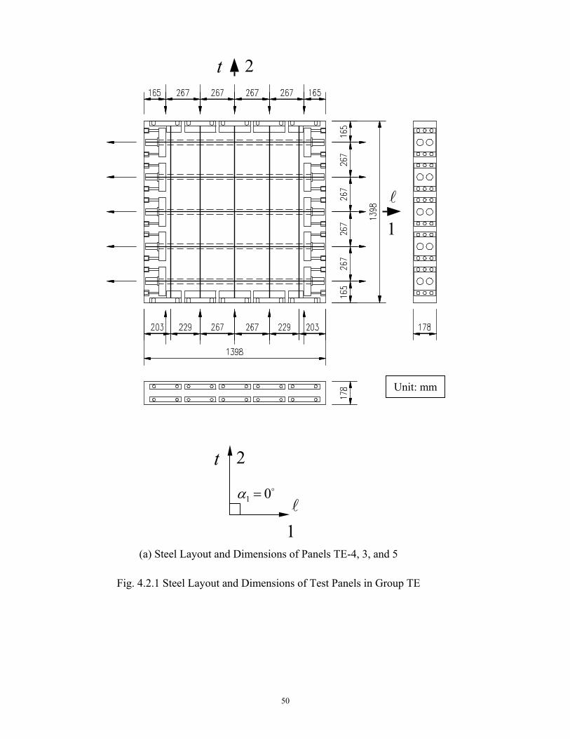
50

(a) Steel Layout and Dimensions of Panels TE-4, 3, and 5

l

1

t 2

t

l

2

1

o01 =α

Fig. 4.2.1 Steel Layout and Dimensions of Test Panels in Group TE

Unit: mm

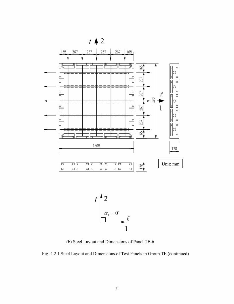
51

t

l

2

1

o01 =α

(b) Steel Layout and Dimensions of Panel TE-6

Fig. 4.2.1 Steel Layout and Dimensions of Test Panels in Group TE (continued)

l

1

t 2

Unit: mm

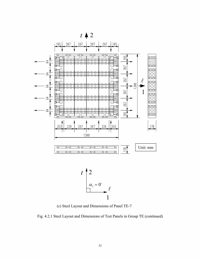
52

t

l

2

1

o01 =α

l

1

t 2

(c) Steel Layout and Dimensions of Panel TE-7

Fig. 4.2.1 Steel Layout and Dimensions of Test Panels in Group TE (continued)

Unit: mm

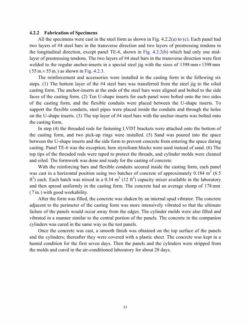
53

4.2.2 Fabrication of Specimens All the specimens were cast in the steel form as shown in Fig. 4.2.2(a) to (c). Each panel had

two layers of #4 steel bars in the transverse direction and two layers of prestressing tendons in the longitudinal direction, except panel TE-6, shown in Fig. 4.2.2(b) which had only one mid-layer of prestressing tendons. The two layers of #4 steel bars in the transverse direction were first welded to the regular anchor-inserts in a special steel jig with the sizes of mm 1398mm 1398 × ( in. 55in. 55 × ) as shown in Fig. 4.2.3.

The reinforcement and accessories were installed in the casting form in the following six steps. (1) The bottom layer of the #4 steel bars was transferred from the steel jig to the oiled casting form. The anchor-inserts at the ends of the steel bars were aligned and bolted to the side faces of the casting form. (2) Ten U-shape inserts for each panel were bolted onto the two sides of the casting form, and the flexible conduits were placed between the U-shape inserts. To support the flexible conduits, steel pipes were placed inside the conduits and through the holes on the U-shape inserts. (3) The top layer of #4 steel bars with the anchor-inserts was bolted onto the casting form.

In step (4) the threaded rods for fastening LVDT brackets were attached onto the bottom of the casting form, and two pick-up rings were installed. (5) Sand was poured into the space between the U-shape inserts and the side form to prevent concrete from entering the space during casting. Panel TE-6 was the exception; here styrofoam blocks were used instead of sand. (6) The top tips of the threaded rods were taped to protect the threads, and cylinder molds were cleaned and oiled. The formwork was done and ready for the casting of concrete. With the reinforcing bars and flexible conduits secured inside the casting form, each panel was cast in a horizontal position using two batches of concrete of approximately 0.184 m3 (6.5 ft3) each. Each batch was mixed in a 0.34 m3 (12 ft3) capacity mixer available in the laboratory and then spread uniformly in the casting form. The concrete had an average slump of mm 178 ( in. 7 ) with good workability. After the form was filled, the concrete was shaken by an internal spud vibrator. The concrete adjacent to the perimeter of the casting form was more intensively vibrated so that the ultimate failure of the panels would occur away from the edges. The cylinder molds were also filled and vibrated in a manner similar to the central portion of the panels. The concrete in the companion cylinders was cured in the same way as the test panels. Once the concrete was cast, a smooth finish was obtained on the top surface of the panels and the cylinders; thereafter they were covered with a plastic sheet. The concrete was kept in a humid condition for the first seven days. Then the panels and the cylinders were stripped from the molds and cured in the air-conditioned laboratory for about 28 days.

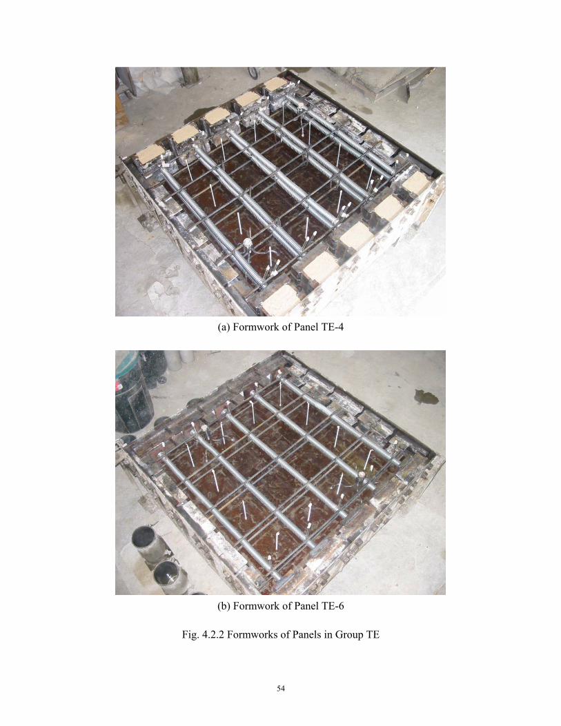
54

Fig. 4.2.2 Formworks of Panels in Group TE

(a) Formwork of Panel TE-4

(b) Formwork of Panel TE-6

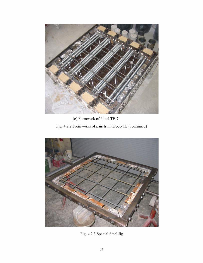
55

Fig. 4.2.3 Special Steel Jig

(c) Formwork of Panel TE-7

Fig. 4.2.2 Formworks of panels in Group TE (continued)

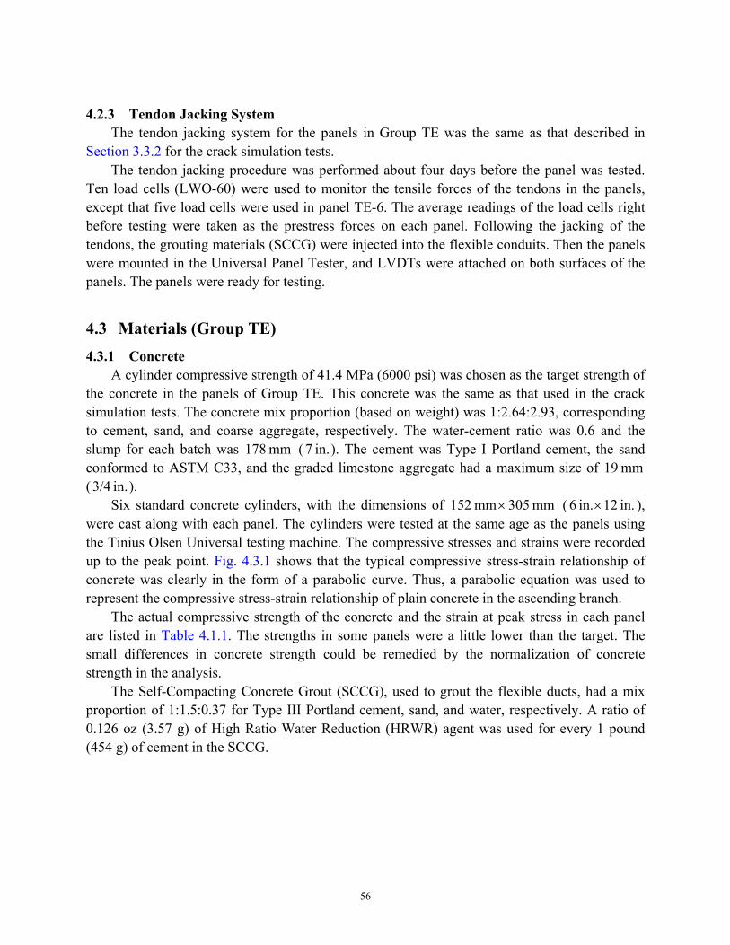
56

4.2.3 Tendon Jacking System

The tendon jacking system for the panels in Group TE was the same as that described in Section 3.3.2 for the crack simulation tests.

The tendon jacking procedure was performed about four days before the panel was tested. Ten load cells (LWO-60) were used to monitor the tensile forces of the tendons in the panels, except that five load cells were used in panel TE-6. The average readings of the load cells right before testing were taken as the prestress forces on each panel. Following the jacking of the tendons, the grouting materials (SCCG) were injected into the flexible conduits. Then the panels were mounted in the Universal Panel Tester, and LVDTs were attached on both surfaces of the panels. The panels were ready for testing.

4.3 Materials (Group TE) 4.3.1 Concrete

A cylinder compressive strength of 41.4 MPa (6000 psi) was chosen as the target strength of the concrete in the panels of Group TE. This concrete was the same as that used in the crack simulation tests. The concrete mix proportion (based on weight) was 1:2.64:2.93, corresponding to cement, sand, and coarse aggregate, respectively. The water-cement ratio was 0.6 and the slump for each batch was mm 178 ( in. 7 ). The cement was Type I Portland cement, the sand conformed to ASTM C33, and the graded limestone aggregate had a maximum size of mm 19 ( in. 3/4 ).

Six standard concrete cylinders, with the dimensions of mm 305mm 152 × ( in. 12in. 6 × ), were cast along with each panel. The cylinders were tested at the same age as the panels using the Tinius Olsen Universal testing machine. The compressive stresses and strains were recorded up to the peak point. Fig. 4.3.1 shows that the typical compressive stress-strain relationship of concrete was clearly in the form of a parabolic curve. Thus, a parabolic equation was used to represent the compressive stress-strain relationship of plain concrete in the ascending branch.

The actual compressive strength of the concrete and the strain at peak stress in each panel are listed in Table 4.1.1. The strengths in some panels were a little lower than the target. The small differences in concrete strength could be remedied by the normalization of concrete strength in the analysis. The Self-Compacting Concrete Grout (SCCG), used to grout the flexible ducts, had a mix proportion of 1:1.5:0.37 for Type III Portland cement, sand, and water, respectively. A ratio of 0.126 oz (3.57 g) of High Ratio Water Reduction (HRWR) agent was used for every 1 pound (454 g) of cement in the SCCG.

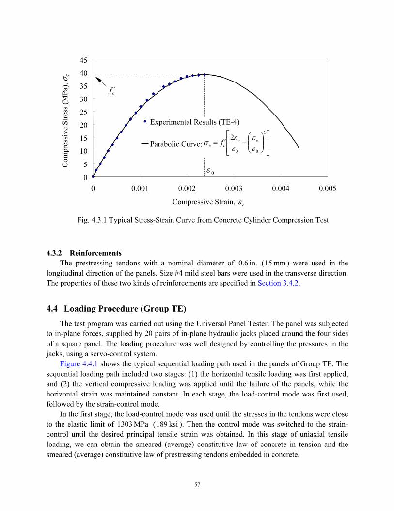
57

4.3.2 Reinforcements The prestressing tendons with a nominal diameter of in. 0.6 ( mm 15 ) were used in the

longitudinal direction of the panels. Size #4 mild steel bars were used in the transverse direction. The properties of these two kinds of reinforcements are specified in Section 3.4.2.

4.4 Loading Procedure (Group TE) The test program was carried out using the Universal Panel Tester. The panel was subjected

to in-plane forces, supplied by 20 pairs of in-plane hydraulic jacks placed around the four sides of a square panel. The loading procedure was well designed by controlling the pressures in the jacks, using a servo-control system.

Figure 4.4.1 shows the typical sequential loading path used in the panels of Group TE. The sequential loading path included two stages: (1) the horizontal tensile loading was first applied, and (2) the vertical compressive loading was applied until the failure of the panels, while the horizontal strain was maintained constant. In each stage, the load-control mode was first used, followed by the strain-control mode.

In the first stage, the load-control mode was used until the stresses in the tendons were close to the elastic limit of MPa 1303 ( ksi 189 ). Then the control mode was switched to the strain-control until the desired principal tensile strain was obtained. In this stage of uniaxial tensile loading, we can obtain the smeared (average) constitutive law of concrete in tension and the smeared (average) constitutive law of prestressing tendons embedded in concrete.

Fig. 4.3.1 Typical Stress-Strain Curve from Concrete Cylinder Compression Test

0

5

10

15

20

25

30

35

40

45

0 0.001 0.002 0.003 0.004 0.005

Compressive Strain, cε

Com

pres

sive

Stre

ss (M

Pa), σ c

0ε

cf ′

Experimental Results (TE-4)

Parabolic Curve:

−′=

2

00

2εε

εεσ cc

cc f

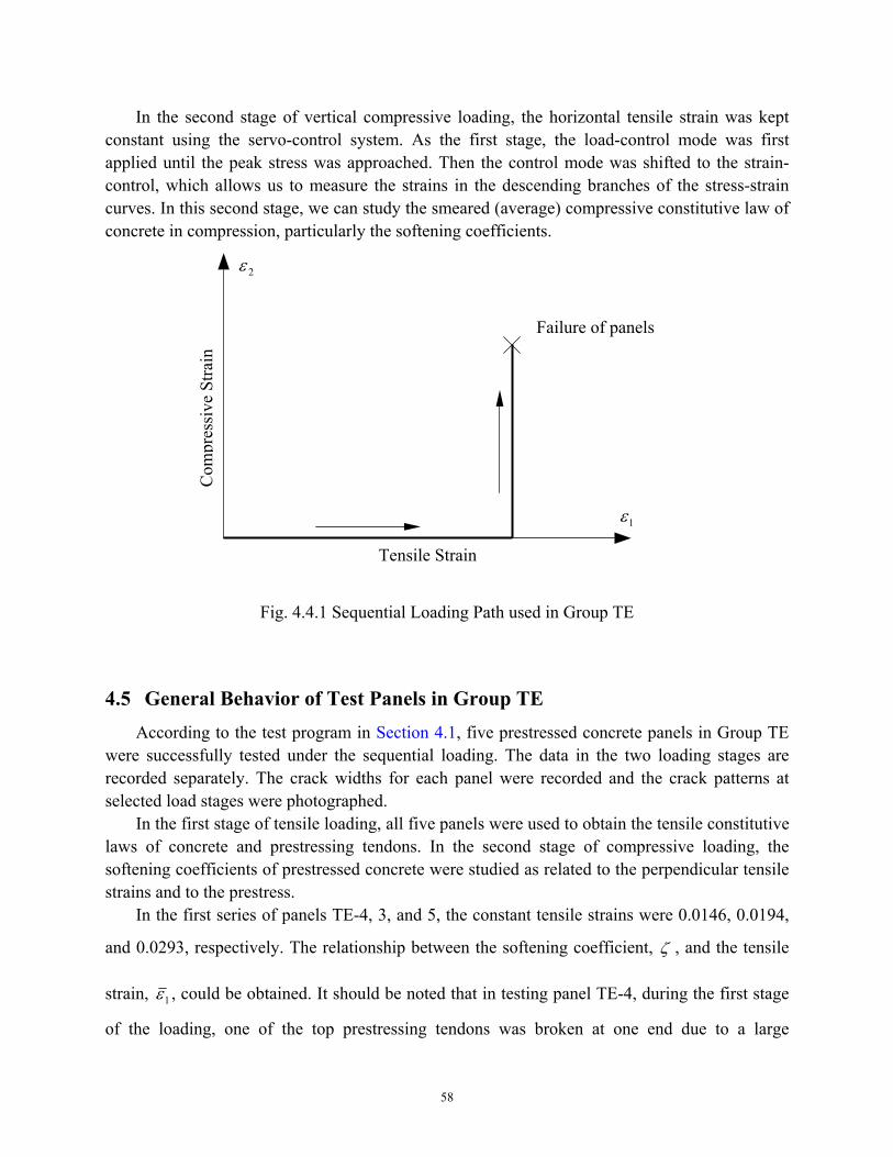
58

In the second stage of vertical compressive loading, the horizontal tensile strain was kept constant using the servo-control system. As the first stage, the load-control mode was first applied until the peak stress was approached. Then the control mode was shifted to the strain-control, which allows us to measure the strains in the descending branches of the stress-strain curves. In this second stage, we can study the smeared (average) compressive constitutive law of concrete in compression, particularly the softening coefficients.

4.5 General Behavior of Test Panels in Group TE According to the test program in Section 4.1, five prestressed concrete panels in Group TE

were successfully tested under the sequential loading. The data in the two loading stages are recorded separately. The crack widths for each panel were recorded and the crack patterns at selected load stages were photographed.

In the first stage of tensile loading, all five panels were used to obtain the tensile constitutive laws of concrete and prestressing tendons. In the second stage of compressive loading, the softening coefficients of prestressed concrete were studied as related to the perpendicular tensile strains and to the prestress.

In the first series of panels TE-4, 3, and 5, the constant tensile strains were 0.0146, 0.0194,

and 0.0293, respectively. The relationship between the softening coefficient, ζ , and the tensile

strain, 1ε , could be obtained. It should be noted that in testing panel TE-4, during the first stage

of the loading, one of the top prestressing tendons was broken at one end due to a large

Fig. 4.4.1 Sequential Loading Path used in Group TE

Com

pres

sive

Stra

in

2ε

1ε

Tensile Strain

Failure of panels

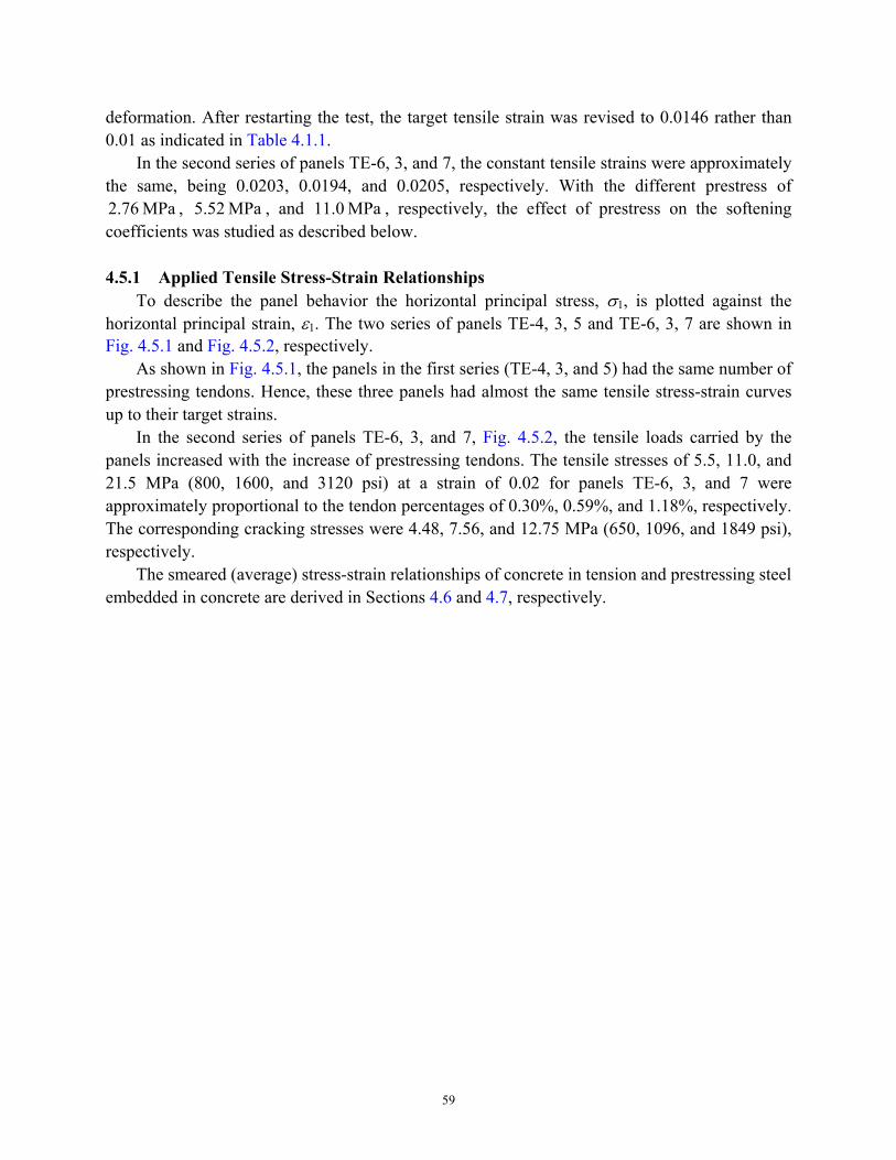
59

deformation. After restarting the test, the target tensile strain was revised to 0.0146 rather than 0.01 as indicated in Table 4.1.1.

In the second series of panels TE-6, 3, and 7, the constant tensile strains were approximately the same, being 0.0203, 0.0194, and 0.0205, respectively. With the different prestress of

MPa 2.76 , MPa 5.52 , and MPa 11.0 , respectively, the effect of prestress on the softening coefficients was studied as described below.

4.5.1 Applied Tensile Stress-Strain Relationships

To describe the panel behavior the horizontal principal stress, σ1, is plotted against the horizontal principal strain, ε1. The two series of panels TE-4, 3, 5 and TE-6, 3, 7 are shown in Fig. 4.5.1 and Fig. 4.5.2, respectively.

As shown in Fig. 4.5.1, the panels in the first series (TE-4, 3, and 5) had the same number of prestressing tendons. Hence, these three panels had almost the same tensile stress-strain curves up to their target strains.

In the second series of panels TE-6, 3, and 7, Fig. 4.5.2, the tensile loads carried by the panels increased with the increase of prestressing tendons. The tensile stresses of 5.5, 11.0, and 21.5 MPa (800, 1600, and 3120 psi) at a strain of 0.02 for panels TE-6, 3, and 7 were approximately proportional to the tendon percentages of 0.30%, 0.59%, and 1.18%, respectively. The corresponding cracking stresses were 4.48, 7.56, and 12.75 MPa (650, 1096, and 1849 psi), respectively.

The smeared (average) stress-strain relationships of concrete in tension and prestressing steel embedded in concrete are derived in Sections 4.6 and 4.7, respectively.

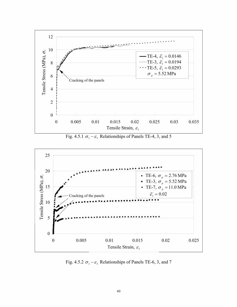
60

0

5

10

15

20

25

0 0.005 0.01 0.015 0.02 0.025Tensile Strain

Tens

ile S

tress

(MPa

)

Fig. 4.5.2 11 εσ − Relationships of Panels TE-6, 3, and 7

Cracking of the panels

Tensile Strain, 1ε

Tens

ile S

tress

(MPa

), σ 1

TE-6, MPa 76.2=pσ TE-3, MPa 52.5=pσ TE-7, MPa 0.11=pσ

02.01 =ε

0

2

4

6

8

10

12

0 0.005 0.01 0.015 0.02 0.025 0.03 0.035Tensile Strain

Tens

ile S

tress

(MPa

) TE-4TE-3TE-5


Cracking of the panels

Tensile Strain, 1ε

Tens

ile S

tress

(MPa

), σ 1

TE-4, 0146.01 =ε TE-3, 0194.01 =ε TE-5, 0293.01 =ε

MPa 5.52=pσ

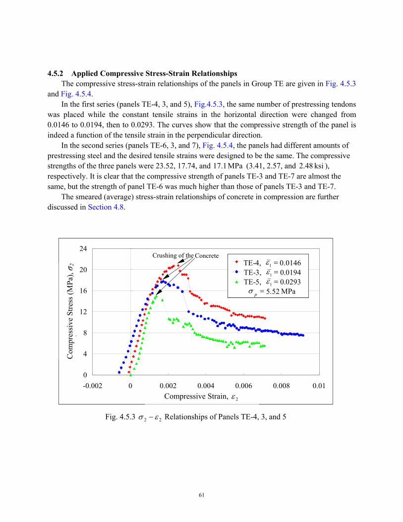
61

4.5.2 Applied Compressive Stress-Strain Relationships The compressive stress-strain relationships of the panels in Group TE are given in Fig. 4.5.3

and Fig. 4.5.4. In the first series (panels TE-4, 3, and 5), Fig.4.5.3, the same number of prestressing tendons

was placed while the constant tensile strains in the horizontal direction were changed from 0.0146 to 0.0194, then to 0.0293. The curves show that the compressive strength of the panel is indeed a function of the tensile strain in the perpendicular direction.

In the second series (panels TE-6, 3, and 7), Fig. 4.5.4, the panels had different amounts of prestressing steel and the desired tensile strains were designed to be the same. The compressive strengths of the three panels were 23.52, 17.74, and MPa 17.1 (3.41, 2.57, and ksi 2.48 ), respectively. It is clear that the compressive strength of panels TE-3 and TE-7 are almost the same, but the strength of panel TE-6 was much higher than those of panels TE-3 and TE-7.

The smeared (average) stress-strain relationships of concrete in compression are further discussed in Section 4.8.

0

4

8

12

16

20

24

-0.002 0 0.002 0.004 0.006 0.008 0.01Compressive Strain

Com

pres

sive

Stre

ss (M

Pa)

TE-4TE-3TE-5


Crushing of the

Compressive Strain, 2ε

Com

pres

sive

Stre

ss (M

Pa), σ 2

TE-4, 0146.01 =εTE-3, 0194.01 =εTE-5, 0293.01 =ε

MPap 52.5=σ

TE-4, 0146.01 =εTE-3, 0194.01 =εTE-5, 0293.01 =ε

MPap 52.5=σ

TE-4, 0146.01 =εTE-3, 0194.01 =εTE-5, 0293.01 =ε

MPap 52.5=σ

Concrete

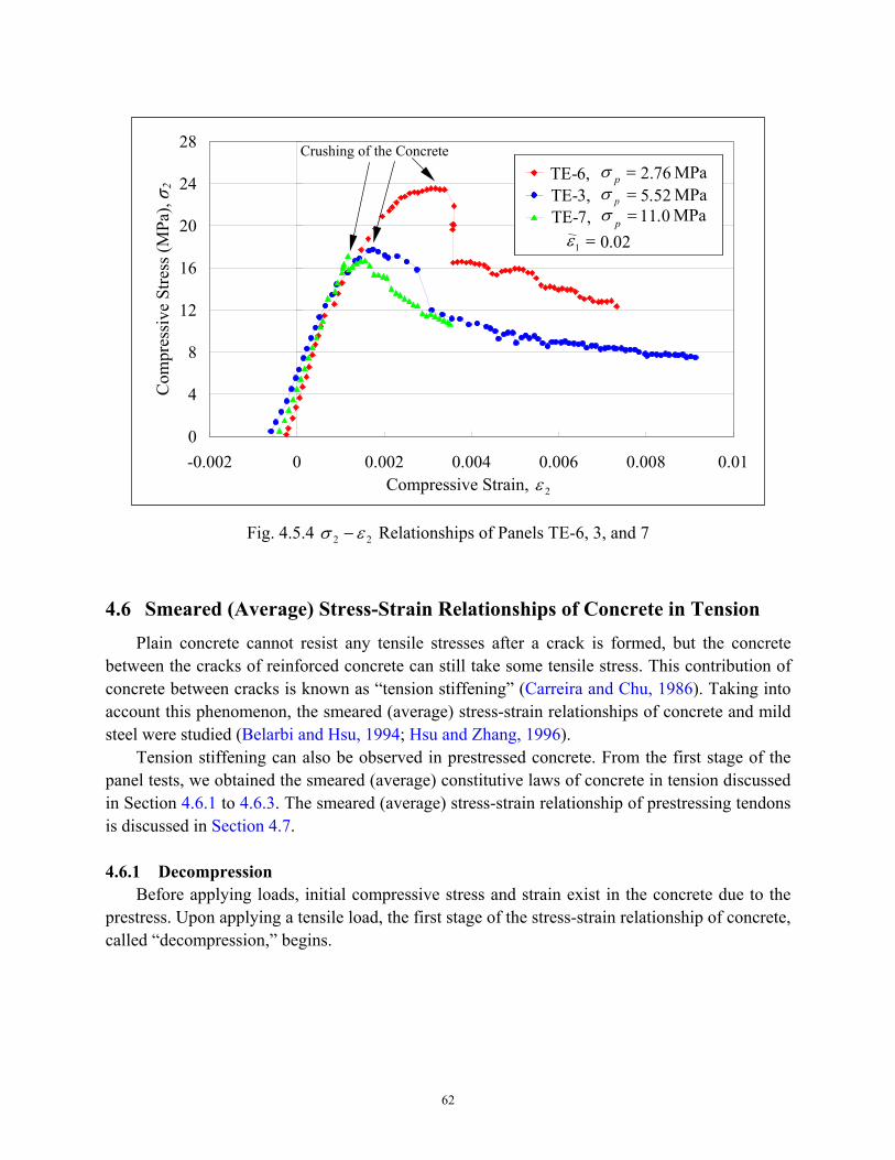
62

4.6 Smeared (Average) Stress-Strain Relationships of Concrete in Tension Plain concrete cannot resist any tensile stresses after a crack is formed, but the concrete

between the cracks of reinforced concrete can still take some tensile stress. This contribution of concrete between cracks is known as “tension stiffening” (Carreira and Chu, 1986). Taking into account this phenomenon, the smeared (average) stress-strain relationships of concrete and mild steel were studied (Belarbi and Hsu, 1994; Hsu and Zhang, 1996).

Tension stiffening can also be observed in prestressed concrete. From the first stage of the panel tests, we obtained the smeared (average) constitutive laws of concrete in tension discussed in Section 4.6.1 to 4.6.3. The smeared (average) stress-strain relationship of prestressing tendons is discussed in Section 4.7.

4.6.1 Decompression

Before applying loads, initial compressive stress and strain exist in the concrete due to the prestress. Upon applying a tensile load, the first stage of the stress-strain relationship of concrete, called “decompression,” begins.

0

4

8

12

16

20

24

28


Com

pres

sive

Stre

ss (M

Pa)

TE-6TE-3TE-7


Crushing of the Concrete

Compressive Strain, 2ε

Com

pres

sive

Stre

ss (M

Pa), σ 2

TE-6, MPap 76.2=σTE-3, MPap 52.5=σTE-7, MPap 0.11=σ

02.01 =ε


02.01 =ε


02.01 =ε

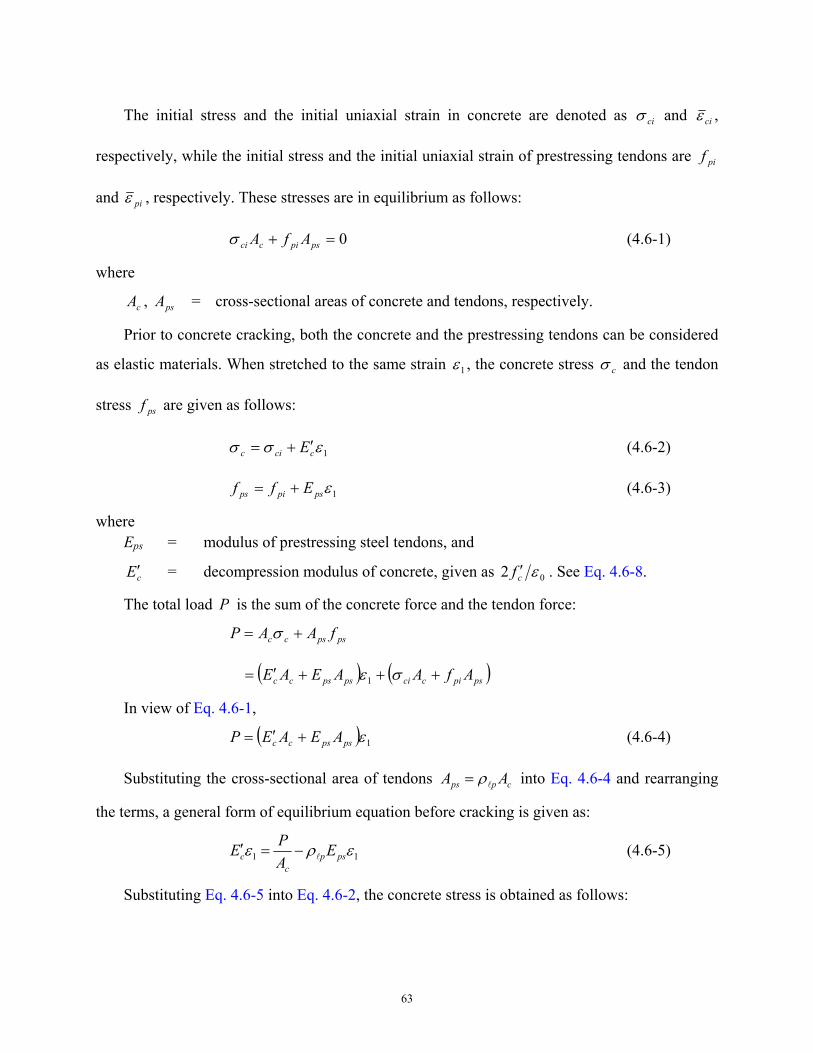
63

The initial stress and the initial uniaxial strain in concrete are denoted as ciσ and ciε ,

respectively, while the initial stress and the initial uniaxial strain of prestressing tendons are pif

and piε , respectively. These stresses are in equilibrium as follows:

0=+ pspicci AfAσ (4.6-1)

where

cA , psA = cross-sectional areas of concrete and tendons, respectively.

Prior to concrete cracking, both the concrete and the prestressing tendons can be considered

as elastic materials. When stretched to the same strain 1ε , the concrete stress cσ and the tendon

stress psf are given as follows:

1εσσ ccic E ′+= (4.6-2)

1εpspips Eff += (4.6-3)

where Eps = modulus of prestressing steel tendons, and

cE ′ = decompression modulus of concrete, given as 02 εcf ′ . See Eq. 4.6-8.

The total load P is the sum of the concrete force and the tendon force:

pspscc fAAP += σ

( ) ( )pspiccipspscc AfAAEAE +++′= σε1

In view of Eq. 4.6-1,

( ) 1εpspscc AEAEP +′= (4.6-4)

Substituting the cross-sectional area of tendons cpps AA lρ= into Eq. 4.6-4 and rearranging

the terms, a general form of equilibrium equation before cracking is given as:

11 ερε pspc

c EAPE l−=′ (4.6-5)

Substituting Eq. 4.6-5 into Eq. 4.6-2, the concrete stress is obtained as follows:

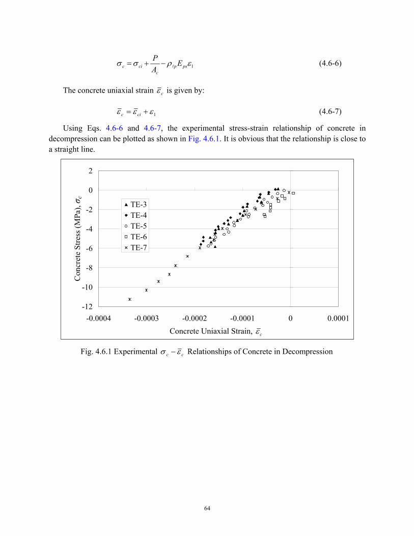
64

1ερσσ pspc

cic EAP

l−+= (4.6-6)

The concrete uniaxial strain cε is given by:

1εεε += cic (4.6-7)

Using Eqs. 4.6-6 and 4.6-7, the experimental stress-strain relationship of concrete in decompression can be plotted as shown in Fig. 4.6.1. It is obvious that the relationship is close to a straight line.

Fig. 4.6.1 Experimental cc εσ − Relationships of Concrete in Decompression

-12

-10

-8

-6

-4

-2

0

2

-0.0004 -0.0003 -0.0002 -0.0001 0 0.0001Strain

Stre

ss (MPa

)

TE-3TE-4TE-5TE-6TE-7

Concrete Uniaxial Strain, cε

Con

cret

e St

ress

(MPa

), σ c

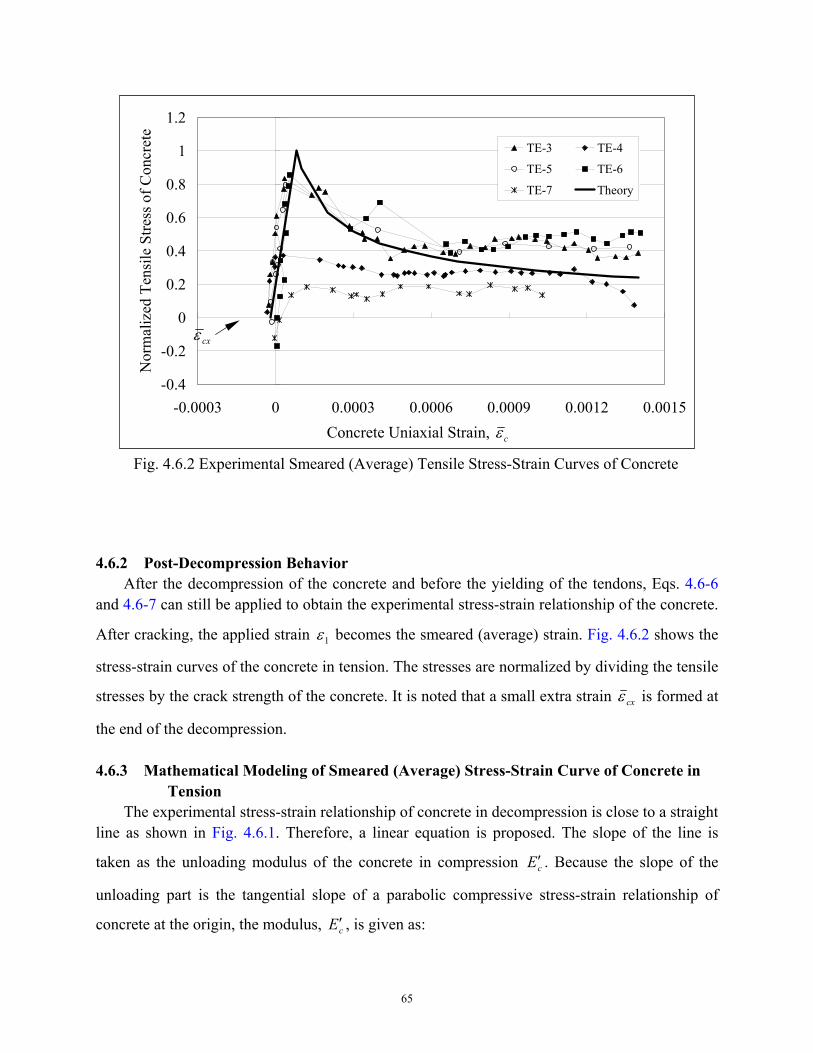
65

4.6.2 Post-Decompression Behavior After the decompression of the concrete and before the yielding of the tendons, Eqs. 4.6-6

and 4.6-7 can still be applied to obtain the experimental stress-strain relationship of the concrete.

After cracking, the applied strain 1ε becomes the smeared (average) strain. Fig. 4.6.2 shows the

stress-strain curves of the concrete in tension. The stresses are normalized by dividing the tensile

stresses by the crack strength of the concrete. It is noted that a small extra strain cxε is formed at

the end of the decompression.

4.6.3 Mathematical Modeling of Smeared (Average) Stress-Strain Curve of Concrete in Tension

The experimental stress-strain relationship of concrete in decompression is close to a straight line as shown in Fig. 4.6.1. Therefore, a linear equation is proposed. The slope of the line is

taken as the unloading modulus of the concrete in compression cE ′ . Because the slope of the

unloading part is the tangential slope of a parabolic compressive stress-strain relationship of

concrete at the origin, the modulus, cE ′ , is given as:

Fig. 4.6.2 Experimental Smeared (Average) Tensile Stress-Strain Curves of Concrete

-0.4

-0.2

0

0.2

0.4

0.6

0.8

1

1.2

-0.0003 0 0.0003 0.0006 0.0009 0.0012 0.0015Strain

Nor

mal

ized

Ten

sile

Stre

ss o

f Con

cret

eTE-3 TE-4

TE-5 TE-6

TE-7 Theory

cxε

Concrete Uniaxial Strain, cε

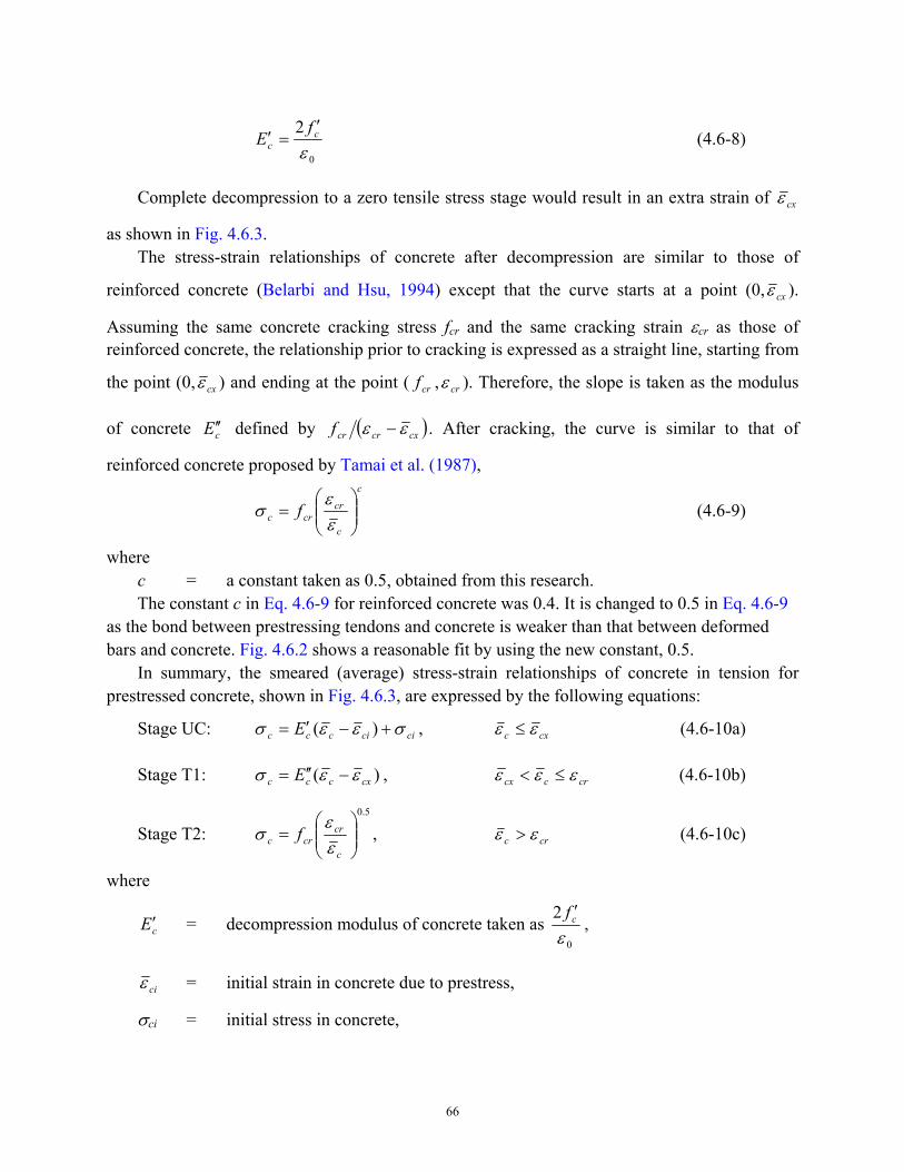
66

0

2εc

cfE

′=′ (4.6-8)

Complete decompression to a zero tensile stress stage would result in an extra strain of cxε

as shown in Fig. 4.6.3. The stress-strain relationships of concrete after decompression are similar to those of

reinforced concrete (Belarbi and Hsu, 1994) except that the curve starts at a point (0, cxε ).

Assuming the same concrete cracking stress fcr and the same cracking strain εcr as those of reinforced concrete, the relationship prior to cracking is expressed as a straight line, starting from

the point (0, cxε ) and ending at the point ( crf , crε ). Therefore, the slope is taken as the modulus

of concrete cE ′′ defined by ( )cxcrcrf εε − . After cracking, the curve is similar to that of

reinforced concrete proposed by Tamai et al. (1987), c

c

crcrc f

=

εε

σ (4.6-9)

where c = a constant taken as 0.5, obtained from this research. The constant c in Eq. 4.6-9 for reinforced concrete was 0.4. It is changed to 0.5 in Eq. 4.6-9

as the bond between prestressing tendons and concrete is weaker than that between deformed bars and concrete. Fig. 4.6.2 shows a reasonable fit by using the new constant, 0.5.

In summary, the smeared (average) stress-strain relationships of concrete in tension for prestressed concrete, shown in Fig. 4.6.3, are expressed by the following equations:

Stage UC: ciciccc E σεεσ +−′= )( , cxc εε ≤ (4.6-10a)

Stage T1: )( cxccc E εεσ −′′= , crccx εεε ≤< (4.6-10b)

Stage T2: 5.0

=

c

crcrc f

εε

σ , crc εε > (4.6-10c)

where

cE ′ = decompression modulus of concrete taken as 0

2εcf ′

,

ciε = initial strain in concrete due to prestress,

σci = initial stress in concrete,

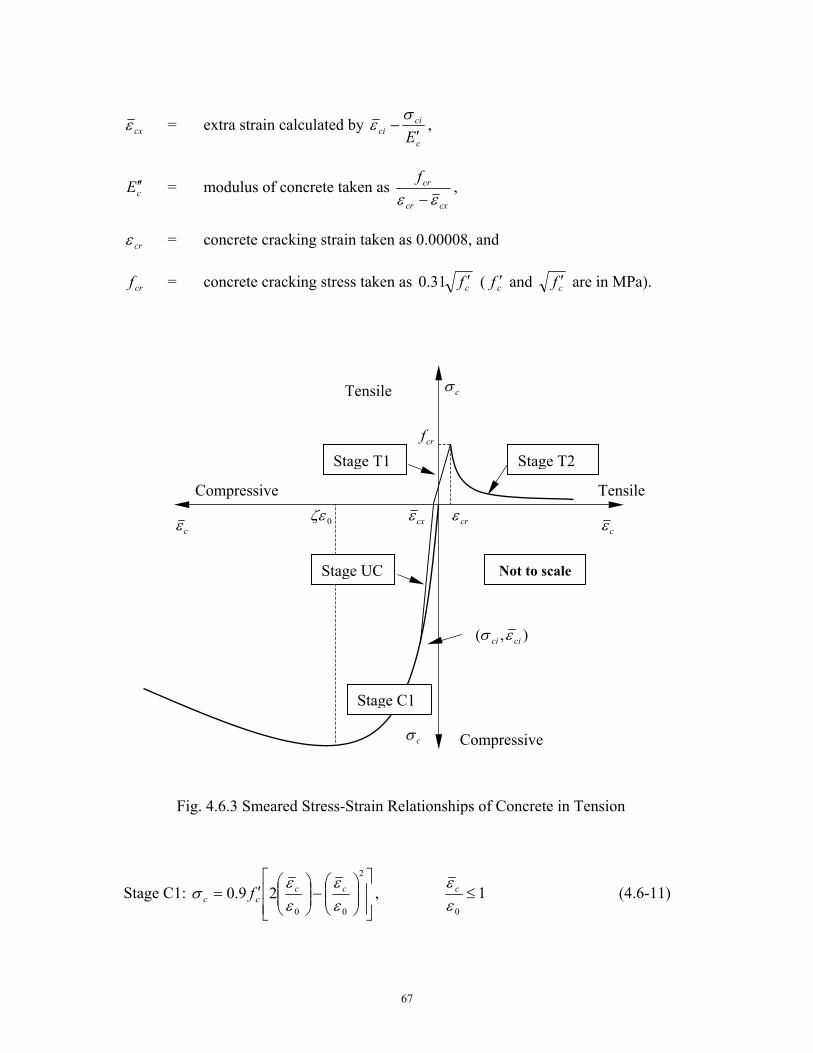
67

cxε = extra strain calculated by c

cici E ′

−σ

ε ,

cE ′′ = modulus of concrete taken as cxcr

crfεε −

,

crε = concrete cracking strain taken as 0.00008, and


Stage C1:

−

′=

2

00

29.0εε

εε

σ cccc f , 1

0

≤εε c (4.6-11)

0ζε

Stage T1

cε cε

cσ

crf

crε

Stage T2

Compressive Tensile

Compressive

Tensile

Not to scale

),( cici εσ

Stage C1

Stage UC

cxε

Fig. 4.6.3 Smeared Stress-Strain Relationships of Concrete in Tension

cσ

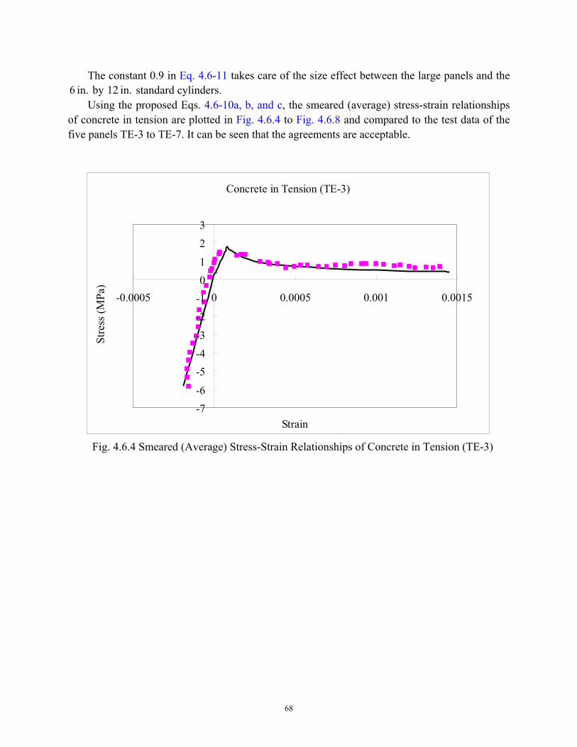
68

The constant 0.9 in Eq. 4.6-11 takes care of the size effect between the large panels and the in. 6 by in. 12 standard cylinders.

Using the proposed Eqs. 4.6-10a, b, and c, the smeared (average) stress-strain relationships of concrete in tension are plotted in Fig. 4.6.4 to Fig. 4.6.8 and compared to the test data of the five panels TE-3 to TE-7. It can be seen that the agreements are acceptable.

Fig. 4.6.4 Smeared (Average) Stress-Strain Relationships of Concrete in Tension (TE-3)

Concrete in Tension (TE-3)

-7-6

-5-4-3

-2-101

23

-0.0005 0 0.0005 0.001 0.0015

Strain

Stre

ss (MPa

)St

ress

(MPa

)

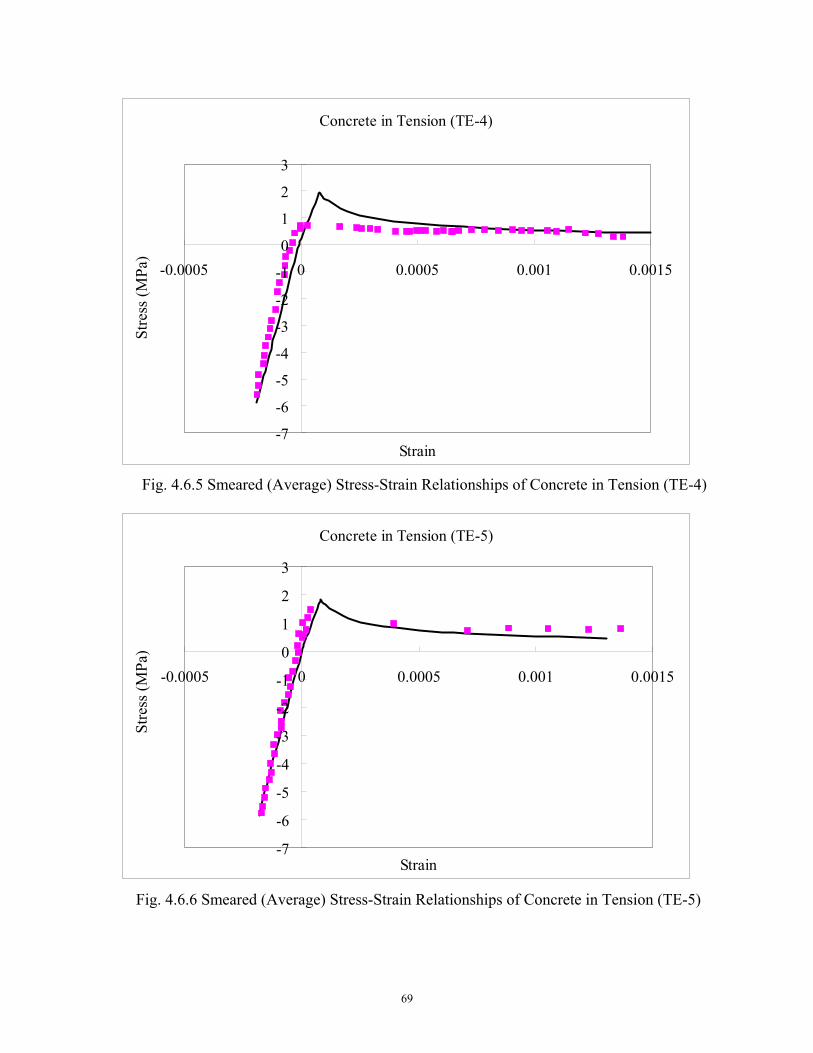
69



-7

-6

-5

-4

-3

-2

-1

0

1

2

3

-0.0005 0 0.0005 0.001 0.0015

Strain

Stre

ss (MPa

)St

ress

(MPa

)



-7

-6

-5

-4

-3

-2

-1

0

1

2

3

-0.0005 0 0.0005 0.001 0.0015

Strain

Stre

ss (MPa

)St

ress

(MPa

)

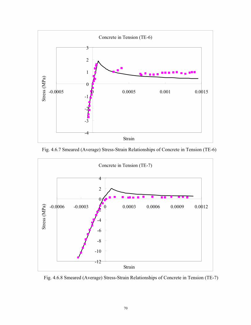
70



-12

-10

-8

-6

-4

-2

0

2

4

-0.0006 -0.0003 0 0.0003 0.0006 0.0009 0.0012

Strain

Stre

ss (MPa

)St

ress

(MPa

)



-4

-3

-2

-1

0

1

2

3

-0.0005 0 0.0005 0.001 0.0015

Strain

Stre

ss (MPa

)St

ress

(MPa

)

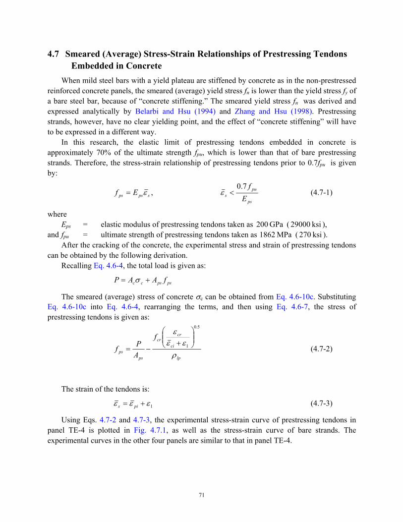
71

4.7 Smeared (Average) Stress-Strain Relationships of Prestressing Tendons Embedded in Concrete

When mild steel bars with a yield plateau are stiffened by concrete as in the non-prestressed reinforced concrete panels, the smeared (average) yield stress fn is lower than the yield stress fy of a bare steel bar, because of “concrete stiffening.” The smeared yield stress fn was derived and expressed analytically by Belarbi and Hsu (1994) and Zhang and Hsu (1998). Prestressing strands, however, have no clear yielding point, and the effect of “concrete stiffening” will have to be expressed in a different way.

In this research, the elastic limit of prestressing tendons embedded in concrete is approximately 70% of the ultimate strength fpu, which is lower than that of bare prestressing strands. Therefore, the stress-strain relationship of prestressing tendons prior to 0.7fpu is given by:

spsps Ef ε= , ps

pus E

f7.0<ε (4.7-1)

where Eps = elastic modulus of prestressing tendons taken as GPa 200 ( ksi 29000 ),

and fpu = ultimate strength of prestressing tendons taken as MPa 1862 ( ksi 270 ). After the cracking of the concrete, the experimental stress and strain of prestressing tendons

can be obtained by the following derivation. Recalling Eq. 4.6-4, the total load is given as:

pspscc fAAP += σ

The smeared (average) stress of concrete σc can be obtained from Eq. 4.6-10c. Substituting Eq. 4.6-10c into Eq. 4.6-4, rearranging the terms, and then using Eq. 4.6-7, the stress of prestressing tendons is given as:

lp

ci

crcr

psps

f

APf

ρεε

ε5.0

1

+

−= (4.7-2)

The strain of the tendons is:

1εεε += pis (4.7-3)

Using Eqs. 4.7-2 and 4.7-3, the experimental stress-strain curve of prestressing tendons in panel TE-4 is plotted in Fig. 4.7.1, as well as the stress-strain curve of bare strands. The experimental curves in the other four panels are similar to that in panel TE-4.

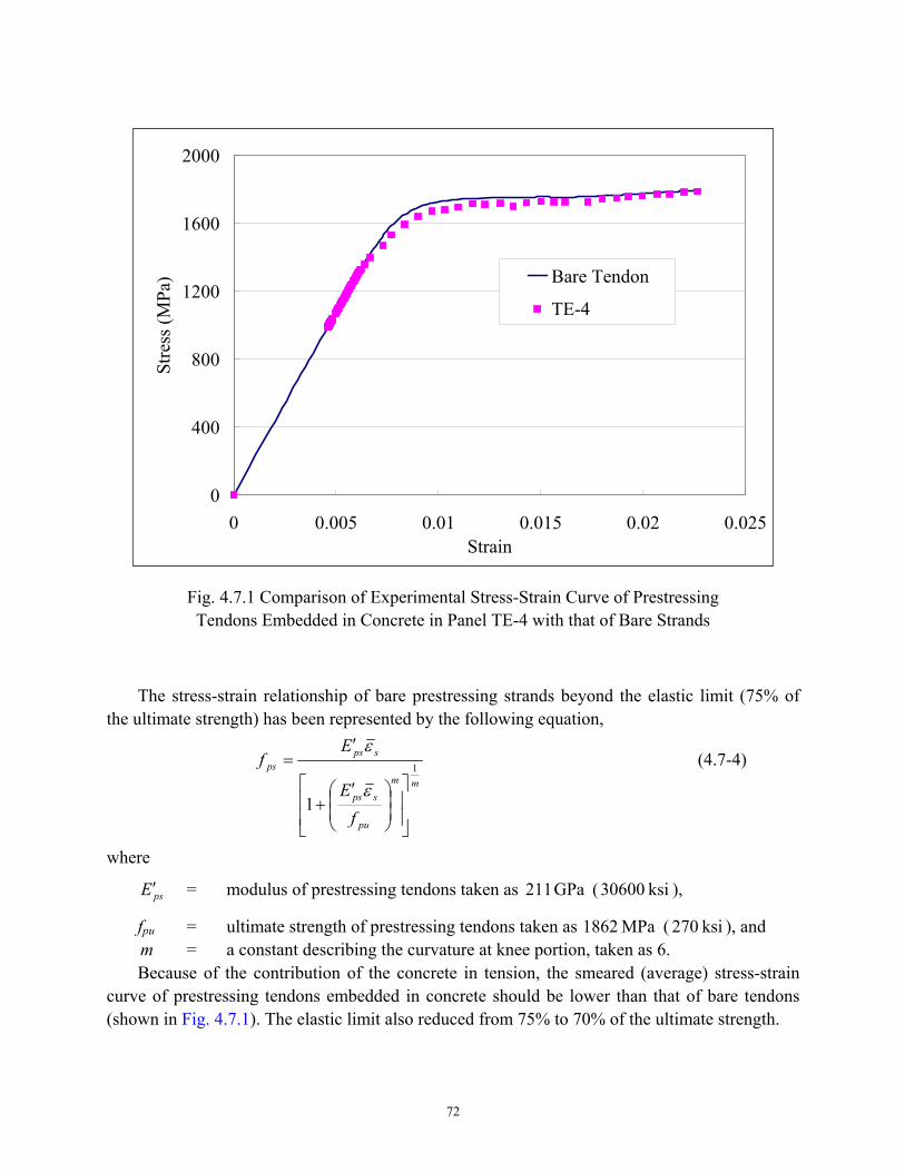
72

The stress-strain relationship of bare prestressing strands beyond the elastic limit (75% of

the ultimate strength) has been represented by the following equation,

mm

pu

sps

spsps

fE

Ef 1

1

′+

′=

ε

ε (4.7-4)

where

psE ′ = modulus of prestressing tendons taken as GPa 211 ( ksi 30600 ),

fpu = ultimate strength of prestressing tendons taken as MPa 1862 ( ksi 270 ), and m = a constant describing the curvature at knee portion, taken as 6. Because of the contribution of the concrete in tension, the smeared (average) stress-strain

curve of prestressing tendons embedded in concrete should be lower than that of bare tendons (shown in Fig. 4.7.1). The elastic limit also reduced from 75% to 70% of the ultimate strength.

Fig. 4.7.1 Comparison of Experimental Stress-Strain Curve of Prestressing Tendons Embedded in Concrete in Panel TE-4 with that of Bare Strands

0

400

800

1200

1600

2000

0 0.005 0.01 0.015 0.02 0.025Strain

Stre

ss (M

Pa) Bare Tendon

TE-4

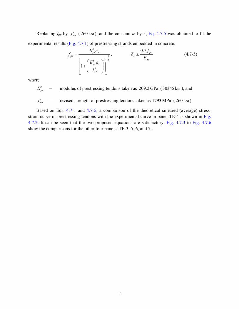
73

Replacing fpu by puf ′ ( ksi 260 ), and the constant m by 5, Eq. 4.7-5 was obtained to fit the

experimental results (Fig. 4.7.1) of prestressing strands embedded in concrete:

51

5

1

′

′′+

′′=

pu

sps

spsps

fE

Ef

ε

ε,

ps

pus E

f7.0≥ε (4.7-5)

where

psE ′′ = modulus of prestressing tendons taken as GPa 209.2 ( ksi 30345 ), and

puf ′ = revised strength of prestressing tendons taken as MPa 7931 ( ksi 260 ).

Based on Eqs. 4.7-1 and 4.7-5, a comparison of the theoretical smeared (average) stress-strain curve of prestressing tendons with the experimental curve in panel TE-4 is shown in Fig. 4.7.2. It can be seen that the two proposed equations are satisfactory. Fig. 4.7.3 to Fig. 4.7.6 show the comparisons for the other four panels, TE-3, 5, 6, and 7.

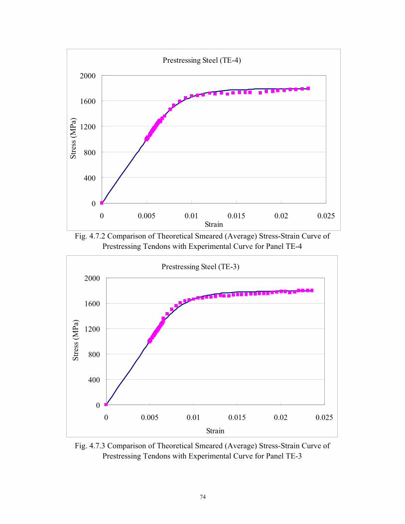
74

Fig. 4.7.2 Comparison of Theoretical Smeared (Average) Stress-Strain Curve of Prestressing Tendons with Experimental Curve for Panel TE-4

Prestressing Steel (TE-4)

0

400

800

1200

1600

2000

0 0.005 0.01 0.015 0.02 0.025Strain

Stre

ss (MPa

)St

ress

(MPa

)



0

400

800

1200

1600

2000

0 0.005 0.01 0.015 0.02 0.025

Strain

Stre

ss (MPa

)St

ress

(MPa

)

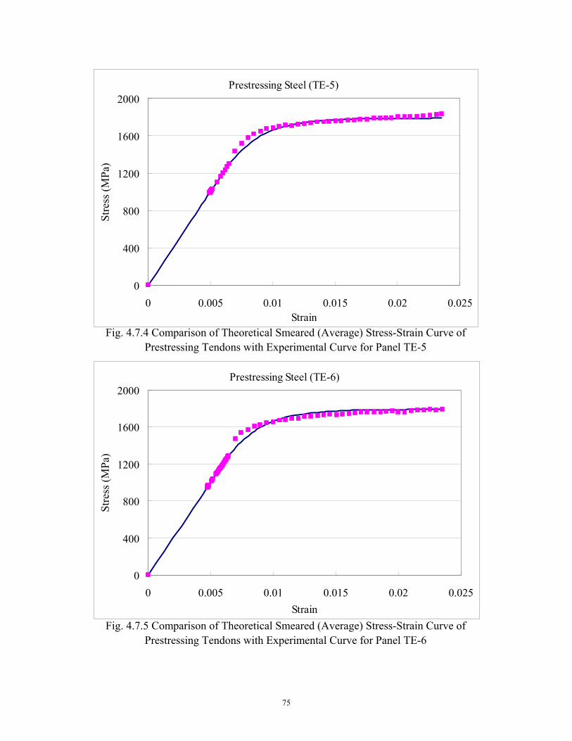
75



0

400

800

1200

1600

2000

0 0.005 0.01 0.015 0.02 0.025Strain

Stre

ss (MPa

)St

ress

(MPa

)



0

400

800

1200

1600

2000

0 0.005 0.01 0.015 0.02 0.025Strain

Stre

ss (MPa

)St

ress

(MPa

)

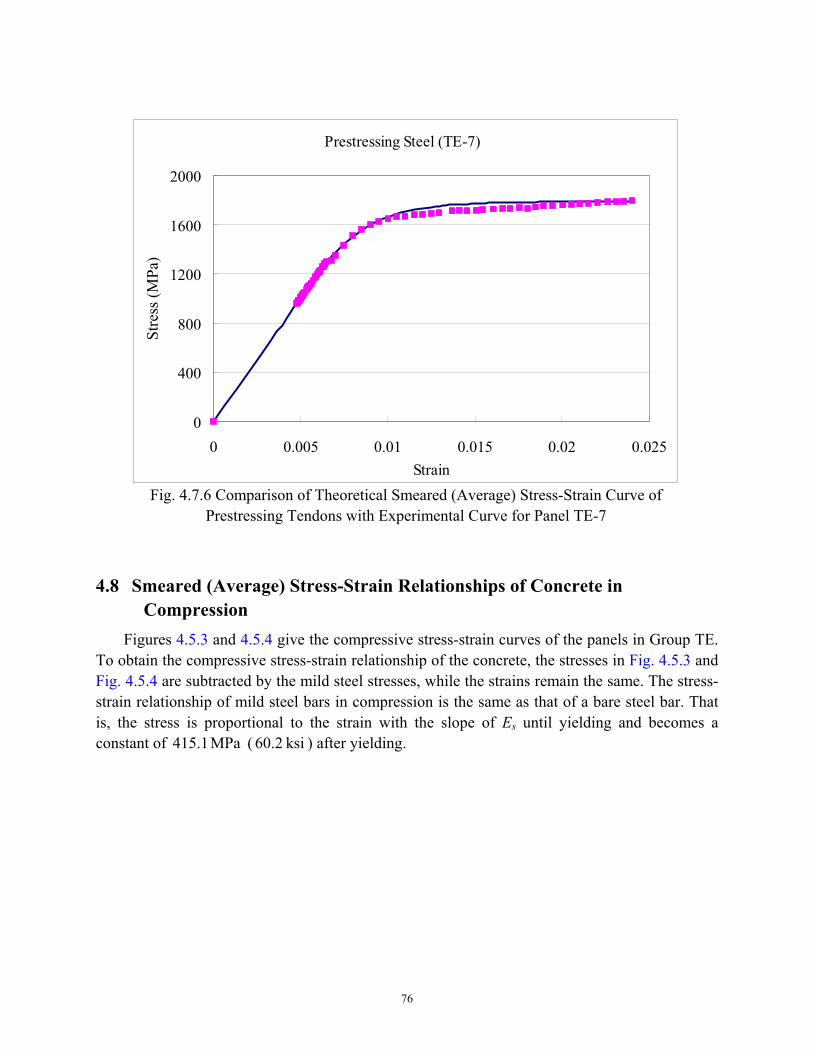
76

4.8 Smeared (Average) Stress-Strain Relationships of Concrete in

Compression Figures 4.5.3 and 4.5.4 give the compressive stress-strain curves of the panels in Group TE.

To obtain the compressive stress-strain relationship of the concrete, the stresses in Fig. 4.5.3 and Fig. 4.5.4 are subtracted by the mild steel stresses, while the strains remain the same. The stress-strain relationship of mild steel bars in compression is the same as that of a bare steel bar. That is, the stress is proportional to the strain with the slope of Es until yielding and becomes a constant of MPa 415.1 ( ksi 60.2 ) after yielding.



0

400

800

1200

1600

2000

0 0.005 0.01 0.015 0.02 0.025Strain

Stre

ss (MPa

)St

ress

(MPa

)

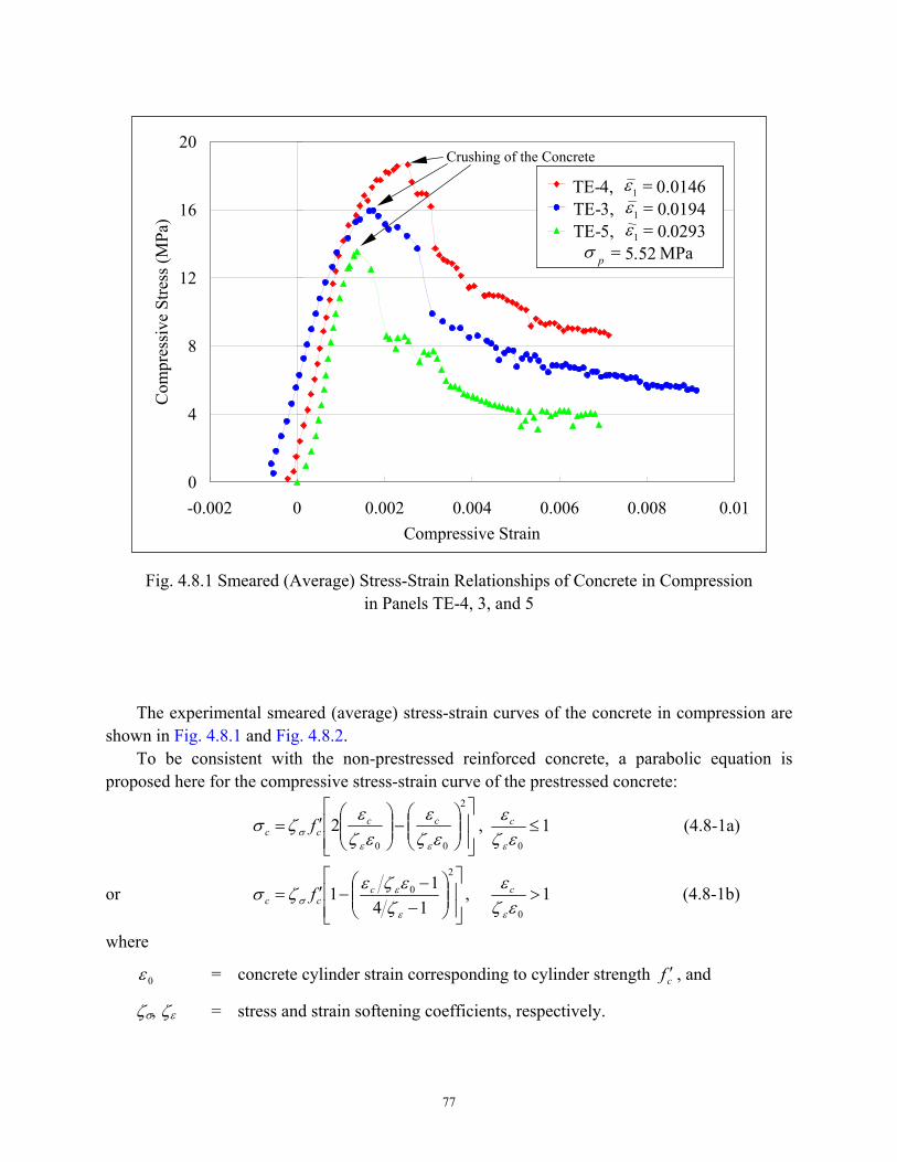
77

The experimental smeared (average) stress-strain curves of the concrete in compression are shown in Fig. 4.8.1 and Fig. 4.8.2.

To be consistent with the non-prestressed reinforced concrete, a parabolic equation is proposed here for the compressive stress-strain curve of the prestressed concrete:

−

′=

2

00

2εζ

εεζ

εζσεε

σcc

cc f , 10

≤εζ

ε

ε

c (4.8-1a)

or

−

−−′=

2

0

1411

ε

εσ ζ

εζεζσ ccc f , 1

0

>εζ

ε

ε

c (4.8-1b)

where

0ε = concrete cylinder strain corresponding to cylinder strength cf ′ , and

ζσ, ζε = stress and strain softening coefficients, respectively.

0

4

8

12

16

20


Com

pres

sive

Stre

ss (M

Pa)

TE-4TE-3TE-5

Fig. 4.8.1 Smeared (Average) Stress-Strain Relationships of Concrete in Compression in Panels TE-4, 3, and 5

Crushing of the Concrete

TE-4, 0146.01 =εTE-3, 0194.01 =εTE-5, 0293.01 =ε

MPap 52.5=σ

TE-4, 0146.01 =εTE-3, 0194.01 =εTE-5, 0293.01 =ε

MPap 52.5=σ

TE-4, 0146.01 =εTE-3, 0194.01 =εTE-5, 0293.01 =ε

MPap 52.5=σ

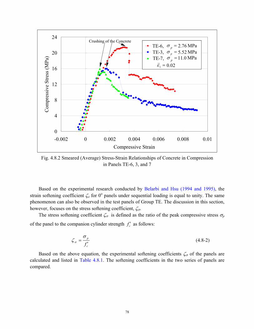
78

Based on the experimental research conducted by Belarbi and Hsu (1994 and 1995), the strain softening coefficient ζε for 0o panels under sequential loading is equal to unity. The same phenomenon can also be observed in the test panels of Group TE. The discussion in this section, however, focuses on the stress softening coefficient, ζσ.

The stress softening coefficient ζσ is defined as the ratio of the peak compressive stress σp

of the panel to the companion cylinder strength cf ′ as follows:

c

p

f ′=

σζ σ (4.8-2)

Based on the above equation, the experimental softening coefficients ζσ of the panels are calculated and listed in Table 4.8.1. The softening coefficients in the two series of panels are compared.

0

4

8

12

16

20

24


Com

pres

sive

Stre

ss (M

Pa)

TE-6TE-3TE-7

Fig. 4.8.2 Smeared (Average) Stress-Strain Relationships of Concrete in Compression in Panels TE-6, 3, and 7

Crushing of the Concrete TE-6, MPap 76.2=σTE-3, MPap 52.5=σTE-7, MPap 0.11=σ

02.01 =ε


02.01 =ε


02.01 =ε

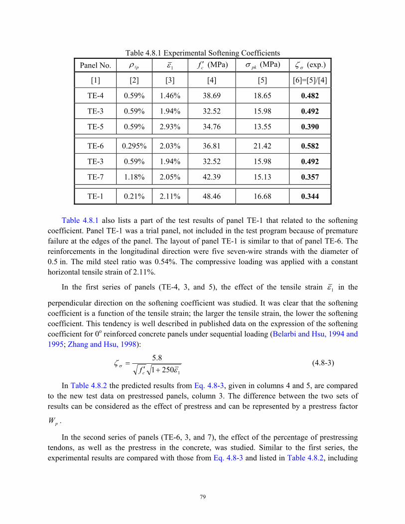
79

Table 4.8.1 Experimental Softening Coefficients Panel No. plρ 1ε cf ′ (MPa) pkσ (MPa) σζ (exp.)

[1] [2] [3] [4] [5] [6]=[5]/[4]

TE-4 0.59% 1.46% 38.69 18.65 0.482

TE-3 0.59% 1.94% 32.52 15.98 0.492

TE-5 0.59% 2.93% 34.76 13.55 0.390

TE-6 0.295% 2.03% 36.81 21.42 0.582

TE-3 0.59% 1.94% 32.52 15.98 0.492

TE-7 1.18% 2.05% 42.39 15.13 0.357

TE-1 0.21% 2.11% 48.46 16.68 0.344

Table 4.8.1 also lists a part of the test results of panel TE-1 that related to the softening

coefficient. Panel TE-1 was a trial panel, not included in the test program because of premature failure at the edges of the panel. The layout of panel TE-1 is similar to that of panel TE-6. The reinforcements in the longitudinal direction were five seven-wire strands with the diameter of 0.5 in. The mild steel ratio was 0.54%. The compressive loading was applied with a constant horizontal tensile strain of 2.11%.

In the first series of panels (TE-4, 3, and 5), the effect of the tensile strain 1ε in the

perpendicular direction on the softening coefficient was studied. It was clear that the softening coefficient is a function of the tensile strain; the larger the tensile strain, the lower the softening coefficient. This tendency is well described in published data on the expression of the softening coefficient for 0o reinforced concrete panels under sequential loading (Belarbi and Hsu, 1994 and 1995; Zhang and Hsu, 1998):

125018.5

εζ σ

+′=

cf (4.8-3)

In Table 4.8.2 the predicted results from Eq. 4.8-3, given in columns 4 and 5, are compared to the new test data on prestressed panels, column 3. The difference between the two sets of results can be considered as the effect of prestress and can be represented by a prestress factor

pW .

In the second series of panels (TE-6, 3, and 7), the effect of the percentage of prestressing tendons, as well as the prestress in the concrete, was studied. Similar to the first series, the experimental results are compared with those from Eq. 4.8-3 and listed in Table 4.8.2, including

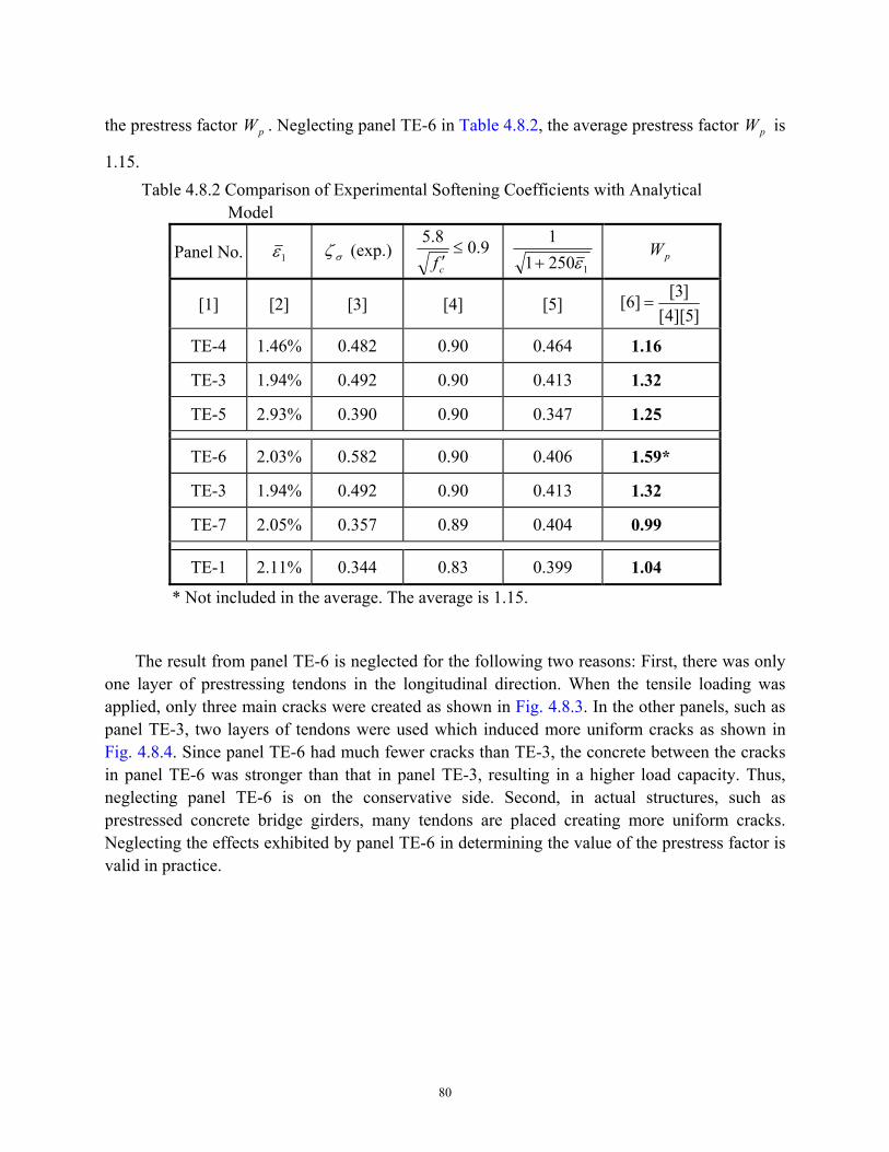
80

the prestress factor pW . Neglecting panel TE-6 in Table 4.8.2, the average prestress factor pW is

1.15.

The result from panel TE-6 is neglected for the following two reasons: First, there was only

one layer of prestressing tendons in the longitudinal direction. When the tensile loading was applied, only three main cracks were created as shown in Fig. 4.8.3. In the other panels, such as panel TE-3, two layers of tendons were used which induced more uniform cracks as shown in Fig. 4.8.4. Since panel TE-6 had much fewer cracks than TE-3, the concrete between the cracks in panel TE-6 was stronger than that in panel TE-3, resulting in a higher load capacity. Thus, neglecting panel TE-6 is on the conservative side. Second, in actual structures, such as prestressed concrete bridge girders, many tendons are placed creating more uniform cracks. Neglecting the effects exhibited by panel TE-6 in determining the value of the prestress factor is valid in practice.

Table 4.8.2 Comparison of Experimental Softening Coefficients with Analytical Model

Panel No. 1ε σζ (exp.) 9.08.5≤

′cf

125011

ε+ pW

[1] [2] [3] [4] [5] ]5][4[]3[]6[ =

TE-4 1.46% 0.482 0.90 0.464 1.16

TE-3 1.94% 0.492 0.90 0.413 1.32

TE-5 2.93% 0.390 0.90 0.347 1.25

TE-6 2.03% 0.582 0.90 0.406 1.59*

TE-3 1.94% 0.492 0.90 0.413 1.32

TE-7 2.05% 0.357 0.89 0.404 0.99

TE-1 2.11% 0.344 0.83 0.399 1.04

* Not included in the average. The average is 1.15.

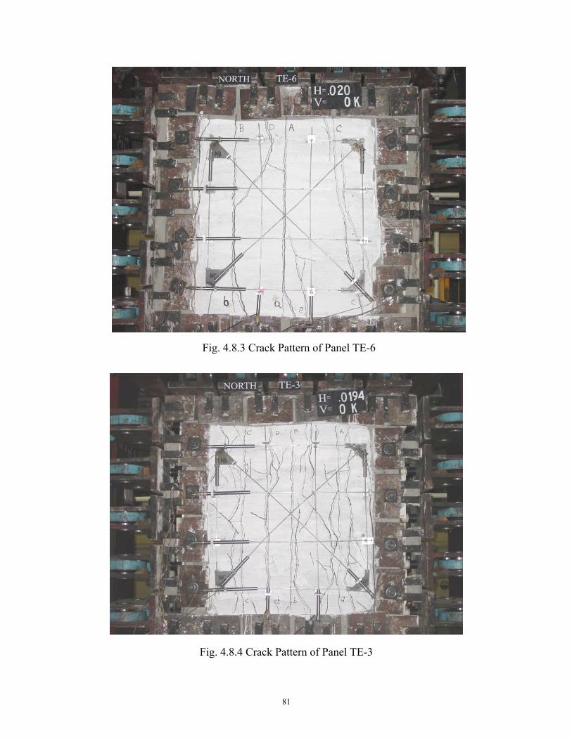
81

Fig. 4.8.4 Crack Pattern of Panel TE-3

Fig. 4.8.3 Crack Pattern of Panel TE-6

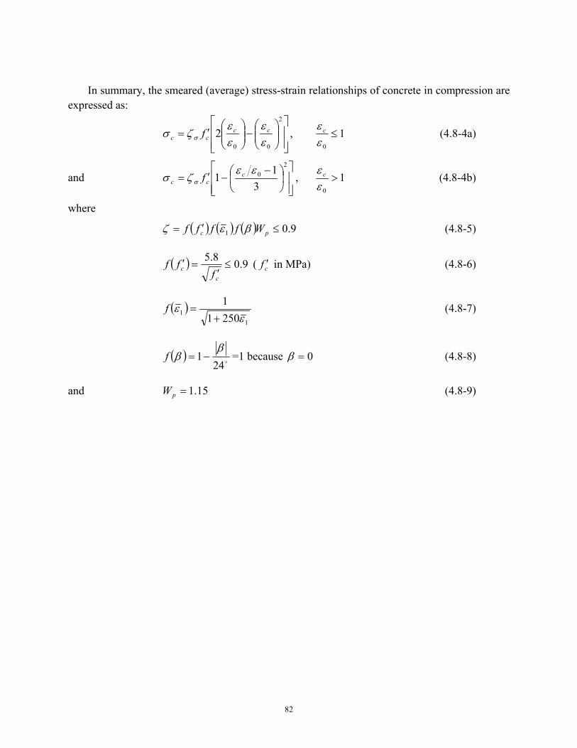
82

In summary, the smeared (average) stress-strain relationships of concrete in compression are

expressed as:

−

′=

2

00

2εε

εε

ζσ σcc

cc f , 10

≤εε c (4.8-4a)

and

−

−′=2

0

31

1εε

ζσ σc

cc f , 10

>εε c (4.8-4b)

where

( ) ( ) ( ) 9.01 ≤′= pc Wffff βεζ (4.8-5)

( ) 9.08.5≤

′=′

cc fff ( cf ′ in MPa) (4.8-6)

( )1

1 25011

εε

+=f (4.8-7)

( )o24

1β

β −=f =1 because 0=β (4.8-8)

and 15.1=pW (4.8-9)

83

CHAPTER 5

PRESTRESSED CONCRETE 45-DEGREE PANELS UNDER PURE

SHEAR (PROPORTIONAL LOADING)

As Chapter 4 describes the test results of the panels in Group TE, Chapter 5 addresses the

studies done on Group TA. Group TA panels with 45o steel bars were subjected to pure shear, a special case of proportional loading. The test program, test specimens, and test results of the panels in Group TA are described. The shear behavior of prestressed concrete was studied, and the stress-strain relationship of concrete in compression is further discussed. Particular attention is given to the new prestress factor in the softening coefficient.

5.1 Test Program (Group TA) Five full-size panels with steel bars oriented at 45o were designed to study the shear behavior

of prestressed concrete membrane elements. Two variables were studied in this group: (1) percentage of prestressing tendons in the longitudinal direction ρlp and (2) percentage of mild steel bars in the transverse direction ρt. The details are listed in Table 5.1.1. The panels in this group are identified first with the letter “T”, which signifies that the panels are designed with prestressing Tendons. The second letter “A” means that the steel grid was oriented at a 45o angle to the applied principal stresses.

The panels in this group were divided into two series based on the two variables. The first series included panels TA-1, 2, and 3. In this series, the percentage of the prestressing steel in the longitudinal direction was kept constant at 0.84%. The mild steel in the transverse direction varied from 0.42% to 0.77% then to 1.54%. The second series included panels TA-2, 4, and 5. The percentages of the mild steel in the transverse direction were 0.77% in the three panels, and the percentages of the prestressing tendons were 0.84%, 0.59%, and 0.42%, respectively. The effects of the percentages of prestressing tendons and the percentage of mild steel on the shear behavior of prestressed concrete membrane elements were studied in the test program.

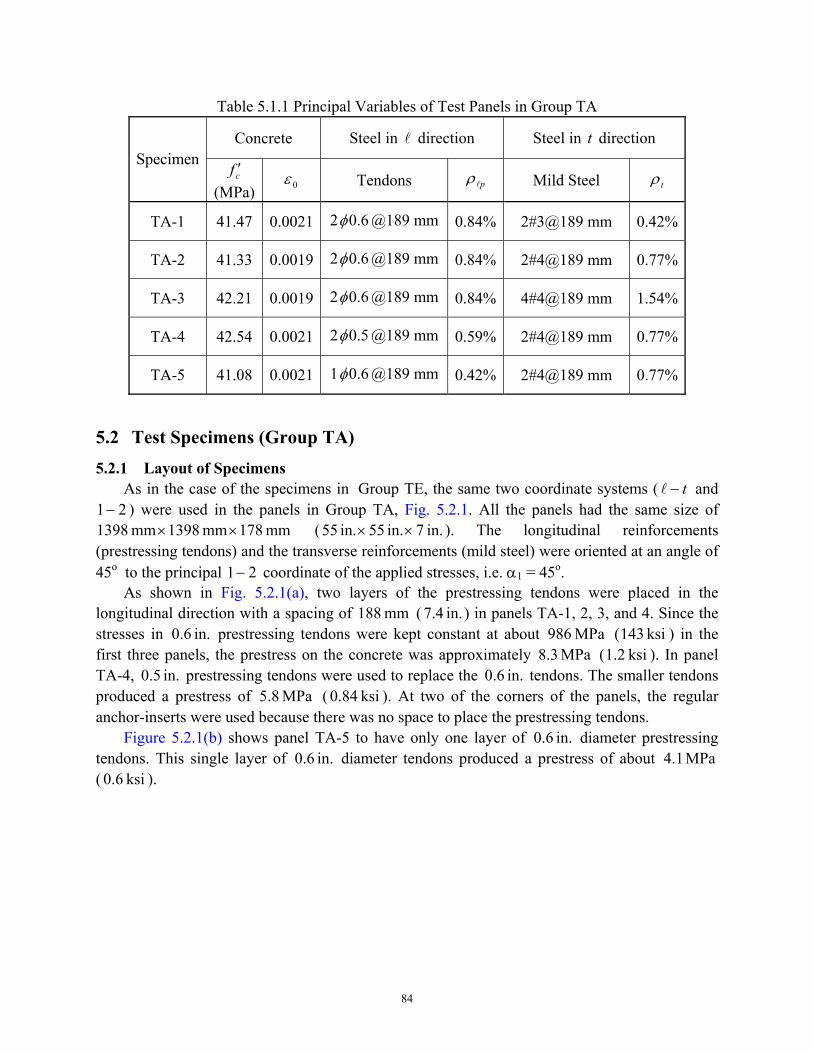
84

Table 5.1.1 Principal Variables of Test Panels in Group TA

Concrete Steel in l direction Steel in t direction Specimen

cf ′ (MPa) 0ε Tendons plρ Mild Steel tρ

TA-1 41.47 0.0021 2 6.0φ @189 mm 0.84% 2#3@189 mm 0.42%

TA-2 41.33 0.0019 2 6.0φ @189 mm 0.84% 2#4@189 mm 0.77%

TA-3 42.21 0.0019 2 6.0φ @189 mm 0.84% 4#4@189 mm 1.54%

TA-4 42.54 0.0021 2 5.0φ @189 mm 0.59% 2#4@189 mm 0.77%

TA-5 41.08 0.0021 1 6.0φ @189 mm 0.42% 2#4@189 mm 0.77%

5.2 Test Specimens (Group TA) 5.2.1 Layout of Specimens

As in the case of the specimens in Group TE, the same two coordinate systems ( t−l and 21− ) were used in the panels in Group TA, Fig. 5.2.1. All the panels had the same size of

mm 178mm 1398mm 1398 ×× ( in. 7in. 55in. 55 ×× ). The longitudinal reinforcements (prestressing tendons) and the transverse reinforcements (mild steel) were oriented at an angle of 45o to the principal 21− coordinate of the applied stresses, i.e. α1 = 45o.

As shown in Fig. 5.2.1(a), two layers of the prestressing tendons were placed in the longitudinal direction with a spacing of mm 188 ( in. 7.4 ) in panels TA-1, 2, 3, and 4. Since the stresses in in. 0.6 prestressing tendons were kept constant at about MPa 986 ( ksi 143 ) in the first three panels, the prestress on the concrete was approximately MPa 8.3 ( ksi .21 ). In panel TA-4, in. 0.5 prestressing tendons were used to replace the in. .60 tendons. The smaller tendons produced a prestress of MPa .85 ( ksi .840 ). At two of the corners of the panels, the regular anchor-inserts were used because there was no space to place the prestressing tendons.

Figure 5.2.1(b) shows panel TA-5 to have only one layer of in. .60 diameter prestressing tendons. This single layer of in. .60 diameter tendons produced a prestress of about MPa .14 ( ksi .60 ).

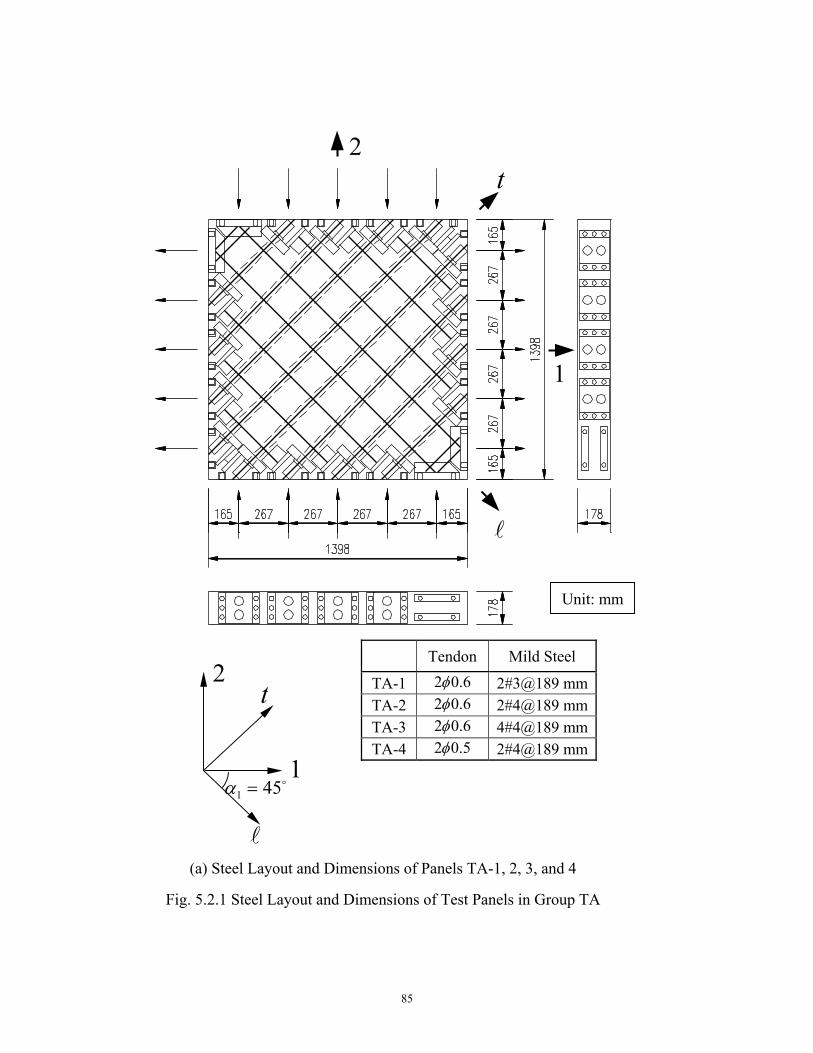
85

t

l

1

2

o451 =α

(a) Steel Layout and Dimensions of Panels TA-1, 2, 3, and 4

l

2t

1

Fig. 5.2.1 Steel Layout and Dimensions of Test Panels in Group TA

Unit: mm

Tendon Mild Steel

TA-1 6.02φ 2#3@189 mm TA-2 6.02φ 2#4@189 mm TA-3 6.02φ 4#4@189 mm TA-4 5.02φ 2#4@189 mm

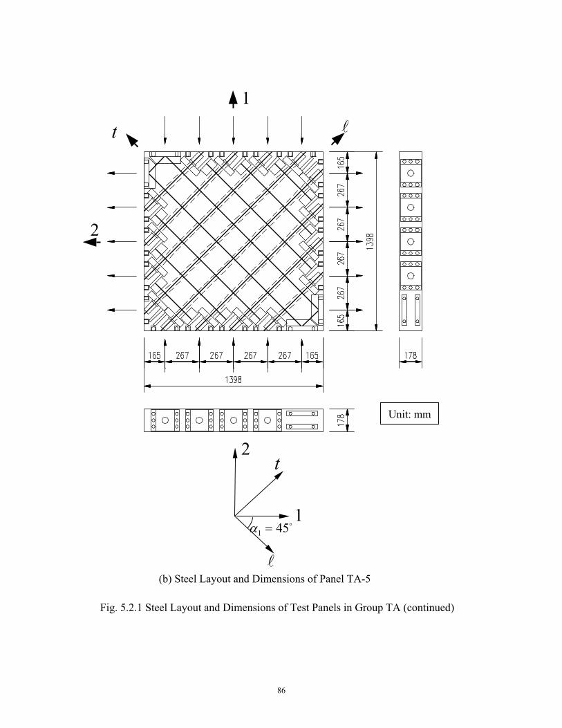
86

(b) Steel Layout and Dimensions of Panel TA-5

l

2

t

1

Fig. 5.2.1 Steel Layout and Dimensions of Test Panels in Group TA (continued)

Unit: mm

t

l

1

2

o451 =α

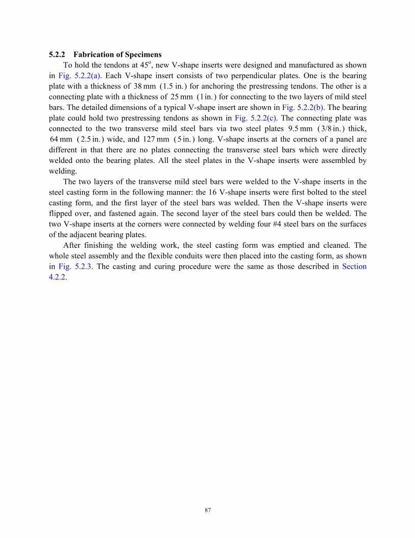
87

5.2.2 Fabrication of Specimens To hold the tendons at 45o, new V-shape inserts were designed and manufactured as shown

in Fig. 5.2.2(a). Each V-shape insert consists of two perpendicular plates. One is the bearing plate with a thickness of mm 38 ( in.5.1 ) for anchoring the prestressing tendons. The other is a connecting plate with a thickness of mm 25 ( in. 1 ) for connecting to the two layers of mild steel bars. The detailed dimensions of a typical V-shape insert are shown in Fig. 5.2.2(b). The bearing plate could hold two prestressing tendons as shown in Fig. 5.2.2(c). The connecting plate was connected to the two transverse mild steel bars via two steel plates mm 9.5 ( in. 3/8 ) thick,

mm 64 ( in. 2.5 ) wide, and mm 127 ( in. 5 ) long. V-shape inserts at the corners of a panel are different in that there are no plates connecting the transverse steel bars which were directly welded onto the bearing plates. All the steel plates in the V-shape inserts were assembled by welding.

The two layers of the transverse mild steel bars were welded to the V-shape inserts in the steel casting form in the following manner: the 16 V-shape inserts were first bolted to the steel casting form, and the first layer of the steel bars was welded. Then the V-shape inserts were flipped over, and fastened again. The second layer of the steel bars could then be welded. The two V-shape inserts at the corners were connected by welding four #4 steel bars on the surfaces of the adjacent bearing plates.

After finishing the welding work, the steel casting form was emptied and cleaned. The whole steel assembly and the flexible conduits were then placed into the casting form, as shown in Fig. 5.2.3. The casting and curing procedure were the same as those described in Section 4.2.2.

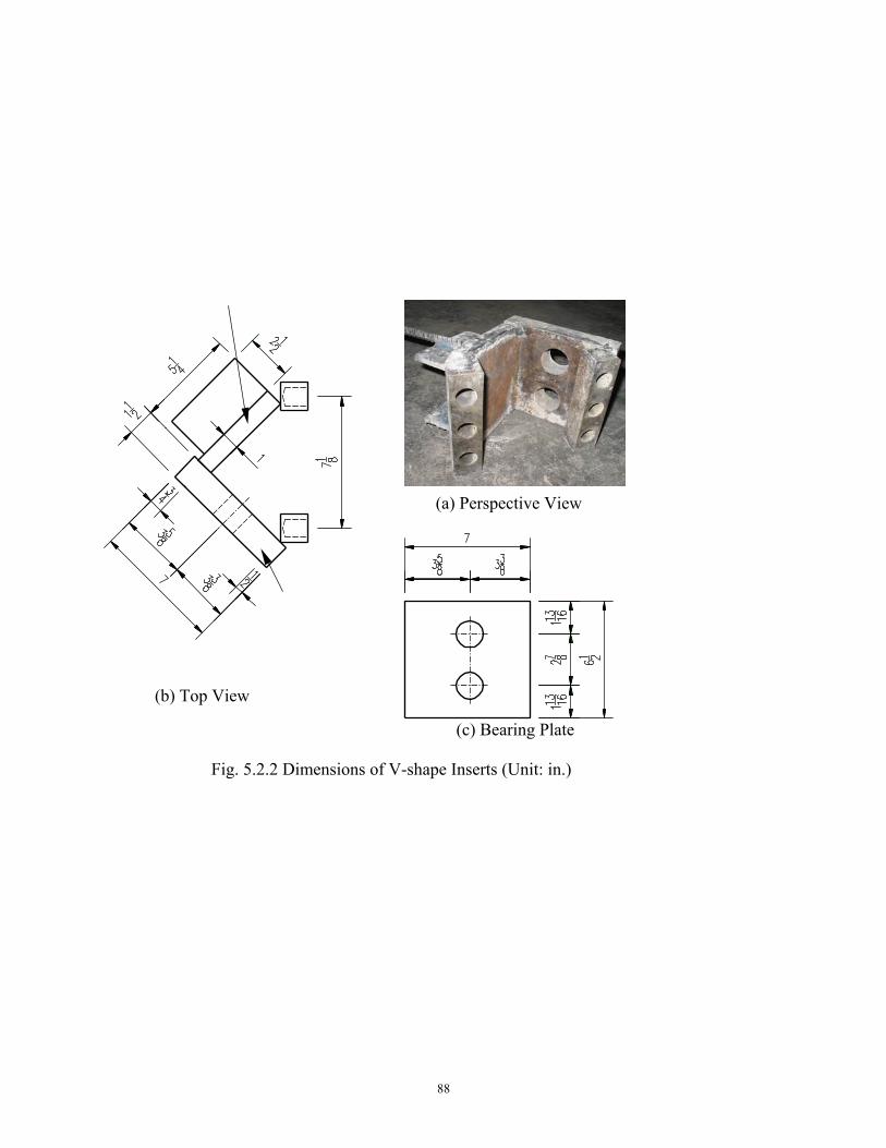
88

Fig. 5.2.2 Dimensions of V-shape Inserts (Unit: in.)

(a) Perspective View

(b) Top View

(c) Bearing Plate

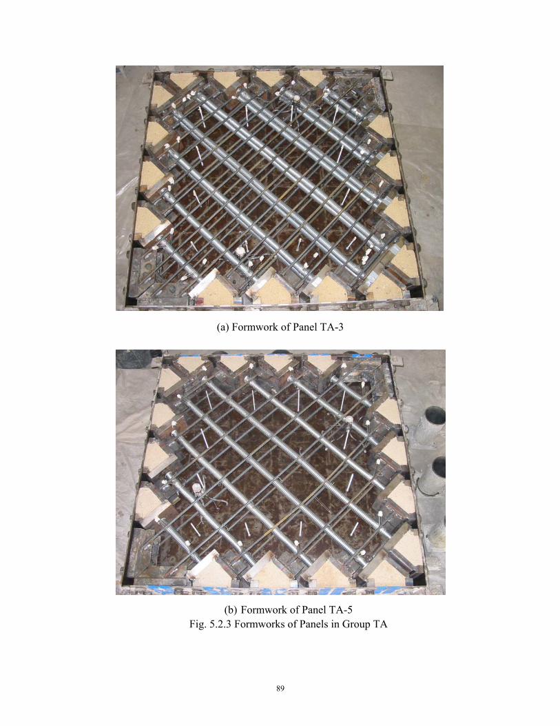
89

(b) Formwork of Panel TA-5 Fig. 5.2.3 Formworks of Panels in Group TA

(a) Formwork of Panel TA-3

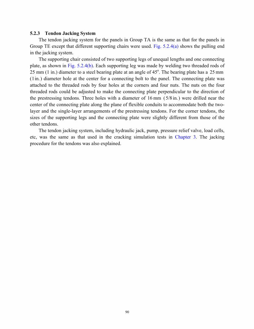
90

5.2.3 Tendon Jacking System The tendon jacking system for the panels in Group TA is the same as that for the panels in

Group TE except that different supporting chairs were used. Fig. 5.2.4(a) shows the pulling end in the jacking system.

The supporting chair consisted of two supporting legs of unequal lengths and one connecting plate, as shown in Fig. 5.2.4(b). Each supporting leg was made by welding two threaded rods of 25 mm (1 in.) diameter to a steel bearing plate at an angle of 45o. The bearing plate has a mm 25 ( in. 1 ) diameter hole at the center for a connecting bolt to the panel. The connecting plate was attached to the threaded rods by four holes at the corners and four nuts. The nuts on the four threaded rods could be adjusted to make the connecting plate perpendicular to the direction of the prestressing tendons. Three holes with a diameter of mm 16 ( in. 5/8 ) were drilled near the center of the connecting plate along the plane of flexible conduits to accommodate both the two-layer and the single-layer arrangements of the prestressing tendons. For the corner tendons, the sizes of the supporting legs and the connecting plate were slightly different from those of the other tendons.

The tendon jacking system, including hydraulic jack, pump, pressure relief valve, load cells, etc, was the same as that used in the cracking simulation tests in Chapter 3. The jacking procedure for the tendons was also explained.

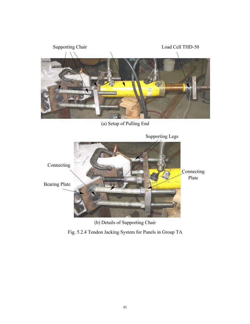
91

Fig. 5.2.4 Tendon Jacking System for Panels in Group TA

Supporting Chair Load Cell THD-50

Bearing Plate

Connecting Plate

Connecting

(a) Setup of Pulling End

(b) Details of Supporting Chair

Supporting Legs

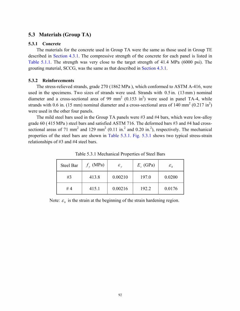
92

5.3 Materials (Group TA) 5.3.1 Concrete

The materials for the concrete used in Group TA were the same as those used in Group TE described in Section 4.3.1. The compressive strength of the concrete for each panel is listed in Table 5.1.1. The strength was very close to the target strength of 41.4 MPa (6000 psi). The grouting material, SCCG, was the same as that described in Section 4.3.1.

5.3.2 Reinforcements

The stress-relieved strands, grade 270 ( MPa 1862 ), which conformed to ASTM A-416, were used in the specimens. Two sizes of strands were used. Strands with in. 0.5 ( mm 13 ) nominal diameter and a cross-sectional area of 99 mm2 (0.153 in2) were used in panel TA-4, while strands with 0.6 in. (15 mm) nominal diameter and a cross-sectional area of 140 mm2 (0.217 in2) were used in the other four panels.

The mild steel bars used in the Group TA panels were #3 and #4 bars, which were low-alloy grade 60 ( MPa 415 ) steel bars and satisfied ASTM 716. The deformed bars #3 and #4 had cross-sectional areas of 71 mm2 and 129 mm2 (0.11 in.2 and 0.20 in.2), respectively. The mechanical properties of the steel bars are shown in Table 5.3.1. Fig. 5.3.1 shows two typical stress-strain relationships of #3 and #4 steel bars.

Table 5.3.1 Mechanical Properties of Steel Bars

Steel Bar yf (MPa) yε sE (GPa) hε

#3 413.8 0.00210 197.0 0.0200

# 4 415.1 0.00216 192.2 0.0176

Note: hε is the strain at the beginning of the strain hardening region.

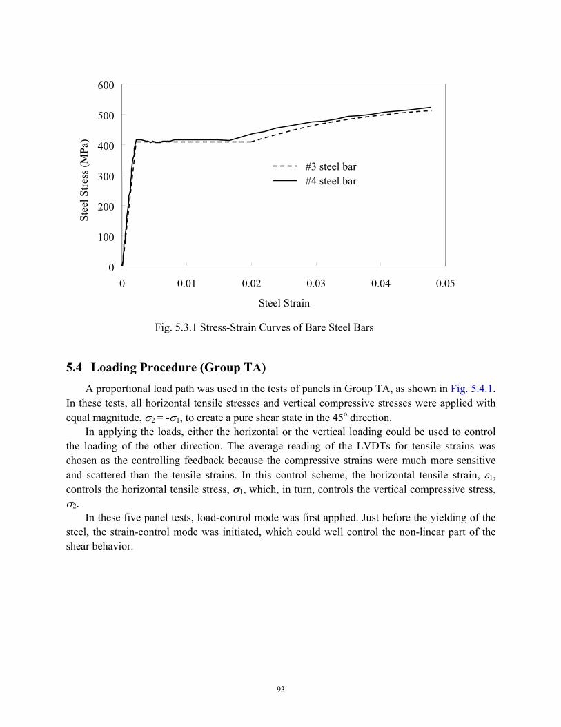
93

5.4 Loading Procedure (Group TA) A proportional load path was used in the tests of panels in Group TA, as shown in Fig. 5.4.1.

In these tests, all horizontal tensile stresses and vertical compressive stresses were applied with equal magnitude, σ2 = -σ1, to create a pure shear state in the 45o direction.

In applying the loads, either the horizontal or the vertical loading could be used to control the loading of the other direction. The average reading of the LVDTs for tensile strains was chosen as the controlling feedback because the compressive strains were much more sensitive and scattered than the tensile strains. In this control scheme, the horizontal tensile strain, ε1, controls the horizontal tensile stress, σ1, which, in turn, controls the vertical compressive stress, σ2.

In these five panel tests, load-control mode was first applied. Just before the yielding of the steel, the strain-control mode was initiated, which could well control the non-linear part of the shear behavior.

Fig. 5.3.1 Stress-Strain Curves of Bare Steel Bars

0

100

200

300

400

500

600

0 0.01 0.02 0.03 0.04 0.05

Steel Strain

Stee

l Stre

ss (M

Pa)

#3 steel bar #4 steel bar

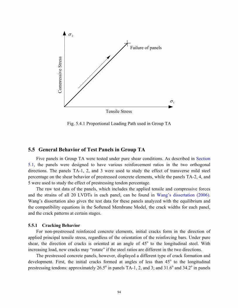
94

5.5 General Behavior of Test Panels in Group TA Five panels in Group TA were tested under pure shear conditions. As described in Section

5.1, the panels were designed to have various reinforcement ratios in the two orthogonal directions. The panels TA-1, 2, and 3 were used to study the effect of transverse mild steel percentage on the shear behavior of prestressed concrete elements, while the panels TA-2, 4, and 5 were used to study the effect of prestressing tendon percentage.

The raw test data of the panels, which includes the applied tensile and compressive forces and the strains of all 20 LVDTs in each panel, can be found in Wang’s dissertation (2006). Wang’s dissertation also gives the test data for these panels analyzed with the equilibrium and the compatibility equations in the Softened Membrane Model, the crack widths for each panel, and the crack patterns at certain stages.

5.5.1 Cracking Behavior

For non-prestressed reinforced concrete elements, initial cracks form in the direction of applied principal tensile stress, regardless of the orientation of the reinforcing bars. Under pure shear, the direction of cracks is oriented at an angle of 45o to the longitudinal steel. With increasing load, new cracks may “rotate” if the steel ratios are different in the two directions.

The prestressed concrete panels, however, displayed a different type of crack formation and development. First, the initial cracks formed at angles of less than 45o to the longitudinal prestressing tendons: approximately 26.5o in panels TA-1, 2, and 3; and 31.6o and 34.2o in panels

Fig. 5.4.1 Proportional Loading Path used in Group TA

Com

pres

sive

Stre

ss

2σ

1σ

Tensile Stress

Failure of panels

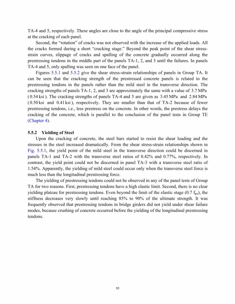
95

TA-4 and 5, respectively. These angles are close to the angle of the principal compressive stress at the cracking of each panel.

Second, the “rotation” of cracks was not observed with the increase of the applied loads. All the cracks formed during a short “cracking stage.” Beyond the peak point of the shear stress-strain curves, slippage of cracks and spalling of the concrete gradually occurred along the prestressing tendons in the middle part of the panels TA-1, 2, and 3 until the failures. In panels TA-4 and 5, only spalling was seen on one face of the panel.

Figures 5.5.1 and 5.5.2 give the shear stress-strain relationships of panels in Group TA. It can be seen that the cracking strength of the prestressed concrete panels is related to the prestressing tendons in the panels rather than the mild steel in the transverse direction. The cracking strengths of panels TA-1, 2, and 3 are approximately the same with a value of MPa 3.7 ( ksi 0.54 ). The cracking strengths of panels TA-4 and 5 are given as MPa 3.45 and MPa 2.84 ( ksi 0.50 and ksi 0.41 ), respectively. They are smaller than that of TA-2 because of fewer prestressing tendons, i.e., less prestress on the concrete. In other words, the prestress delays the cracking of the concrete, which is parallel to the conclusion of the panel tests in Group TE (Chapter 4).

5.5.2 Yielding of Steel

Upon the cracking of concrete, the steel bars started to resist the shear loading and the stresses in the steel increased dramatically. From the shear stress-strain relationships shown in Fig. 5.5.1, the yield point of the mild steel in the transverse direction could be discerned in panels TA-1 and TA-2 with the transverse steel ratios of 0.42% and 0.77%, respectively. In contrast, the yield point could not be discerned in panel TA-3 with a transverse steel ratio of 1.54%. Apparently, the yielding of mild steel could occur only when the transverse steel force is much less than the longitudinal prestressing force.

The yielding of prestressing tendons could not be observed in any of the panel tests of Group TA for two reasons. First, prestressing tendons have a high elastic limit. Second, there is no clear yielding plateau for prestressing tendons. Even beyond the limit of the elastic stage (0.7 fpu), the stiffness decreases very slowly until reaching 85% to 90% of the ultimate strength. It was frequently observed that prestressing tendons in bridge girders did not yield under shear failure modes, because crushing of concrete occurred before the yielding of the longitudinal prestressing tendons.

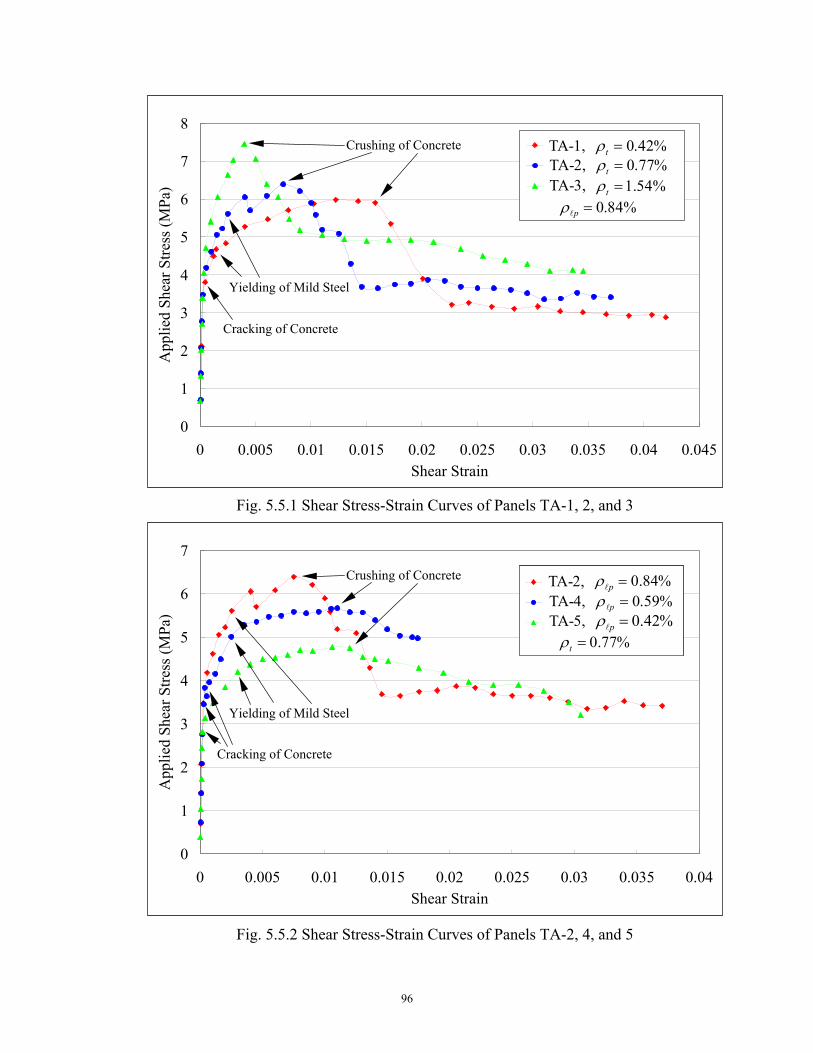
96

0

1

2

3

4

5

6

7

0 0.005 0.01 0.015 0.02 0.025 0.03 0.035 0.04Shear Strain

App

lied

Shea

r Stre

ss (M

Pa)

TA-2TA-4TA-5

0

1

2

3

4

5

6

7

8

0 0.005 0.01 0.015 0.02 0.025 0.03 0.035 0.04 0.045Shear Strain

App

lied

Shea

r Stre

ss (M

Pa)

TA-1TA-2TA-3

Fig. 5.5.1 Shear Stress-Strain Curves of Panels TA-1, 2, and 3

Crushing of Concrete

Cracking of Concrete

Yielding of Mild Steel




Fig. 5.5.2 Shear Stress-Strain Curves of Panels TA-2, 4, and 5

TA-1, %42.0=tρ TA-2, %77.0=tρ TA-3, %54.1=tρ

%84.0=plρ

TA-2, %84.0=plρTA-4, %59.0=plρTA-5, %42.0=plρ

%77.0=tρ


%77.0=tρ

97

5.5.3 Shear Stress vs. Shear Strain Relationships ( tt ll γτ − Curves)

In the five panels, TA-1 to TA-5, the prestressing tendons and the mild steel were oriented at an angle of 45o to the principal 21− coordinate of the applied stresses, i.e. a1 = 45o.

The stress transformation equations of the element in terms of principal applied stresses are given as:

12

212

1 sincos ασασσ +=l (5.5-1)

12

212

1 cossin ασασσ +=t (5.5-2)

1121 cossin)( αασστ +−=tl (5.5-3)

The strain transformation equations of the element in terms of principal strains are given as:

12

212

1 sincos αεαεε +=l (5.5-4)

12

212

1 cossin αεαεε +=t (5.5-5)

1121 cossin)( ααεεγ +−=tl (5.5-6)

Substituting α1 = 45o into Eqs. 5.5-3 and 5.5-6, the shear stress tlτ and the shear strain tlγ

of the element can be calculated by the following simple equation in terms of the principal

stresses and strains ( 2σ , 1σ , 2ε , and 1ε ):

( )2121 σστ +−=tl (5.5-7)

( )2121 εεγ +−=tl (5.5-8)

The principal stresses and strains were calculated using the readings from jack load cells and LVDTs, respectively. The shear stress-strain curves of the panels in the two series are plotted in Fig. 5.5.1 and Fig. 5.5.2, respectively.

As described in Section 5.5.2, each of the curves for panels TA-1, 2, 4, and 5 exhibits three critical points, namely, cracking of concrete, yielding of transverse mild steel, and crushing of concrete. Before the cracking of the concrete, the shear behavior of the panels was elastic and the

tt ll γτ − curves were essentially linear. After cracking, the approximately linear increase of the

shear stresses continued with smaller slopes until the yielding of the mild steel. After the mild steel yielded, the shear strains increased dramatically with a very small increase of shear stresses. The prestressed concrete panels reached their peak shear strengths when the crushing of the

98

concrete occurred. The shear stresses started to decline with the increase of the deformations beyond the peak points.

Test panel TA-3 exhibited a different shear behavior from the other panels. Because this panel had the highest percentages of prestressing tendons and mild steel, the steel in both longitudinal and transverse directions did not yield. There were only two critical points, the cracking and the crushing of the concrete, that divided the shear stress-strain curve into three stages.

From the two series of curves, it is obvious that the maximum shear capacity of the prestressed concrete panels is related to its reinforcement ratios. The experimental shear strengths of the test panels TA-1, 2, and 3 are MPa 5.96 , MPa 6.40 , and MPa 7.47 ( ksi 0.86 ,

ksi 0.93 , and ksi 1.08 ), respectively. The shear strengths are MPa 6.40 , MPa 5.67 , and MPa 4.77 ( ksi 0.93 , ksi 0.82 , and ksi 0.69 ) for test panels TA-2, 4, and 5, respectively. The

shear strength increases with an increase of either prestressing tendon or mild steel ratios. The shear ductility factor is defined as the ratio of the strain at 80% of peak stress in the

descending branch to the strain at the yielding point. It is evident from Fig. 5.5.1 and Fig. 5.5.2 that a prestressed concrete element subjected to shear could exhibit good ductility if properly reinforced. The ductility factors of the panels TA-1, 2, and 3 in the first series are 12.7, 5.0, and less than 1.0 (no steel yielding in panel TA-3), respectively. It is obvious that the ductility increases dramatically with the decrease of the mild steel ratios in the transverse direction. In the second series, the ductility factors are 5.0, 6.9, and 8.6 for panels TA-2, 4, and 5, respectively. The strain at 87% of peak stress is used because of the limited test data for panel TA-4. Obviously, the ductility increases with the reduction of prestressing tendons in the longitudinal direction.

The descending branches of those shear stress-strain curves right after the crushing of the concrete exhibit an interesting phenomenon. In panels TA-1 and TA-2, after the crushing of concrete, the shear stresses dropped rapidly below 80% of peak stress in a short period. Even under strain-control mode, only one or two points within this period were caught. In panels TA-4 and 5, however, there was no sudden drop after the crushing of concrete. The shear stresses gradually decreased with the increase of the shear strains.

5.5.4 Shear Stress vs. Principal Tensile Strain Relationships ( 1ετ −tl Curves)

Figures 5.5.3 and 5.5.4 show the experimental shear stress vs. principal tensile strain

relationships. The principal tensile strains, 1ε , of the prestressed concrete panels are obtained by

averaging the horizontal LVDT readings.

The shapes of the two figures are similar to Figs. 5.5.1 and 5.5.2 because the shear strain tlγ

is governed predominantly by the principal tensile strain, especially before the crushing of the

concrete. Each 1ετ −tl curve also has four stages jointed by three characteristic points. The first

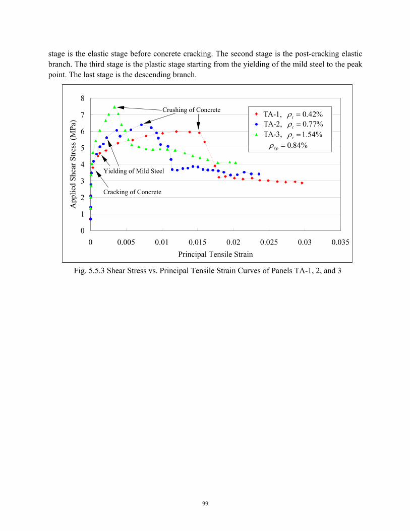
99

stage is the elastic stage before concrete cracking. The second stage is the post-cracking elastic branch. The third stage is the plastic stage starting from the yielding of the mild steel to the peak point. The last stage is the descending branch.

0

1

2

3

4

5

6

7

8

0 0.005 0.01 0.015 0.02 0.025 0.03 0.035Principal Tensile Strain

App

lied

Shea

r Stre

ss (M

Pa)

TA-1TA-2TA-3

Fig. 5.5.3 Shear Stress vs. Principal Tensile Strain Curves of Panels TA-1, 2, and 3




TA-1, %42.0=tρ TA-2, %77.0=tρ TA-3, %54.1=tρ

%84.0=plρ

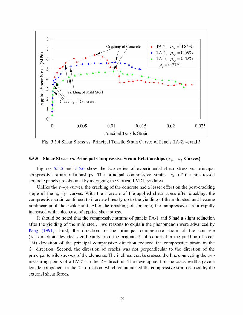
100

5.5.5 Shear Stress vs. Principal Compressive Strain Relationships ( 2ετ −tl Curves)

Figures 5.5.5 and 5.5.6 show the two series of experimental shear stress vs. principal compressive strain relationships. The principal compressive strains, ε2, of the prestressed concrete panels are obtained by averaging the vertical LVDT readings.

Unlike the τlt−γlt curves, the cracking of the concrete had a lesser effect on the post-cracking slope of the τlt−ε2 curves. With the increase of the applied shear stress after cracking, the compressive strain continued to increase linearly up to the yielding of the mild steel and became nonlinear until the peak point. After the crushing of concrete, the compressive strain rapidly increased with a decrease of applied shear stress.

It should be noted that the compressive strains of panels TA-1 and 5 had a slight reduction after the yielding of the mild steel. Two reasons to explain the phenomenon were advanced by Pang (1991). First, the direction of the principal compressive strain of the concrete ( −d direction) deviated significantly from the original −2 direction after the yielding of steel. This deviation of the principal compressive direction reduced the compressive strain in the −2 direction. Second, the direction of cracks was not perpendicular to the direction of the

principal tensile stresses of the elements. The inclined cracks crossed the line connecting the two measuring points of a LVDT in the −2 direction. The development of the crack widths gave a tensile component in the −2 direction, which counteracted the compressive strain caused by the external shear forces.

0

1

2

3

4

5

6

7

8

0 0.005 0.01 0.015 0.02 0.025Principal Tensile Strain

App

lied

Shea

r Stre

ss (M

Pa)

TA-2TA-4TA-5

Fig. 5.5.4 Shear Stress vs. Principal Tensile Strain Curves of Panels TA-2, 4, and 5




TA-2, %84.0=plρ TA-4, %59.0=plρ TA-5, %42.0=plρ

%77.0=tρ


%77.0=tρ

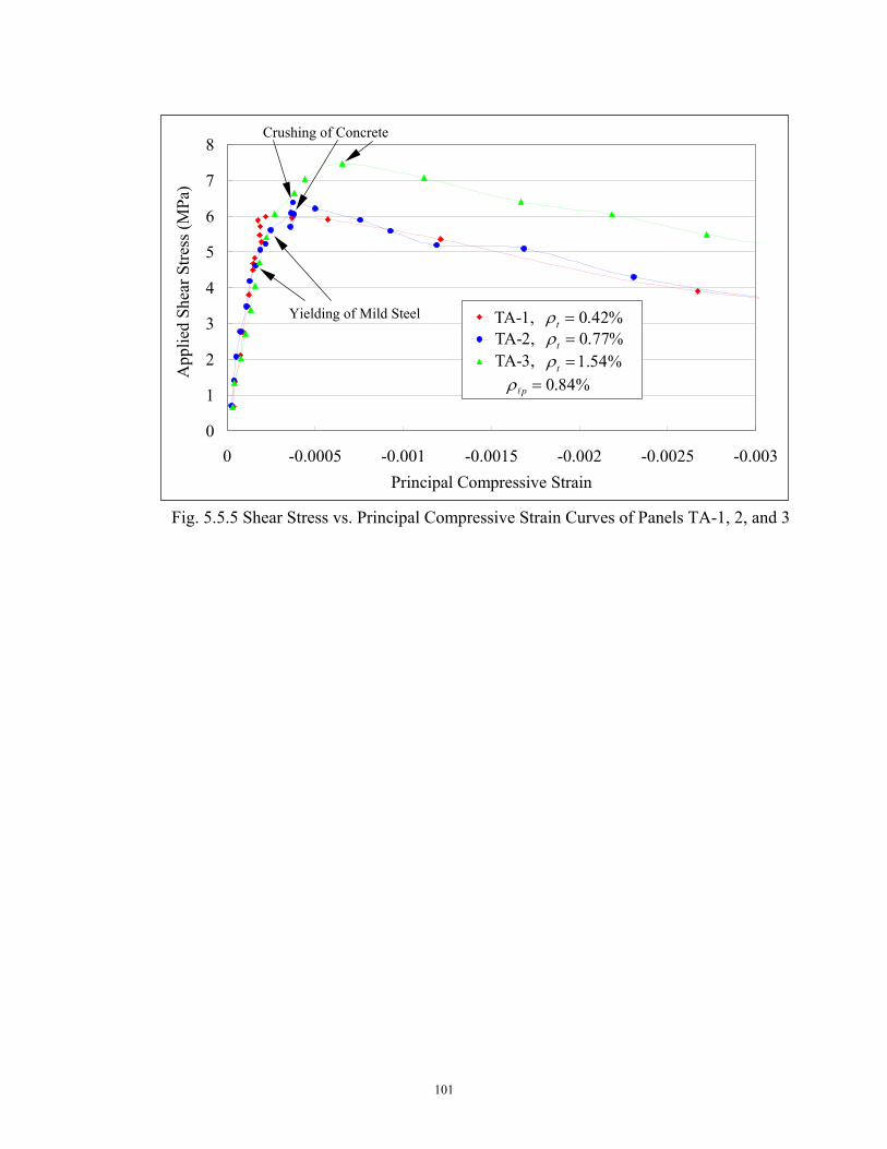
101

0

1

2

3

4

5

6

7

8

-0.003-0.0025-0.002-0.0015-0.001-0.00050Principal Compressive Strain

App

lied

Shea

r Stre

ss (M

Pa)

TA-1TA-2TA-3

Fig. 5.5.5 Shear Stress vs. Principal Compressive Strain Curves of Panels TA-1, 2, and 3


Yielding of Mild Steel TA-1, %42.0=tρ TA-2, %77.0=tρ TA-3, %54.1=tρ

%84.0=plρ

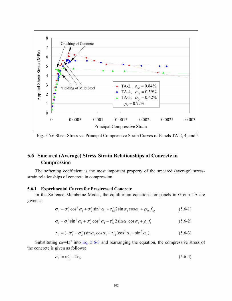
102

5.6 Smeared (Average) Stress-Strain Relationships of Concrete in

Compression The softening coefficient is the most important property of the smeared (average) stress-

strain relationships of concrete in compression.

5.6.1 Experimental Curves for Prestressed Concrete In the Softened Membrane Model, the equilibrium equations for panels in Group TA are

given as:

ppccc flll ραατασασσ +++= 11121

221


ttccc


212


)sin(coscossin)( 12

12

121121 ααταασστ −++−= ccctl (5.6-3)

Substituting α1=45o into Eq. 5.6-3 and rearranging the equation, the compressive stress of the concrete is given as follows:

tcc

lτσσ 221 −= (5.6-4)

0

1

2

3

4

5

6

7

8

-0.003-0.0025-0.002-0.0015-0.001-0.00050Principal Compressive Strain

App

lied

Shea

r Stre

ss (M

Pa)

TA-2TA-4TA-5

Fig. 5.5.6 Shear Stress vs. Principal Compressive Strain Curves of Panels TA-2, 4, and 5


Yielding of Mild Steel TA-2, %84.0=plρTA-4, %59.0=plρTA-5, %42.0=plρ

%77.0=tρ


%77.0=tρ

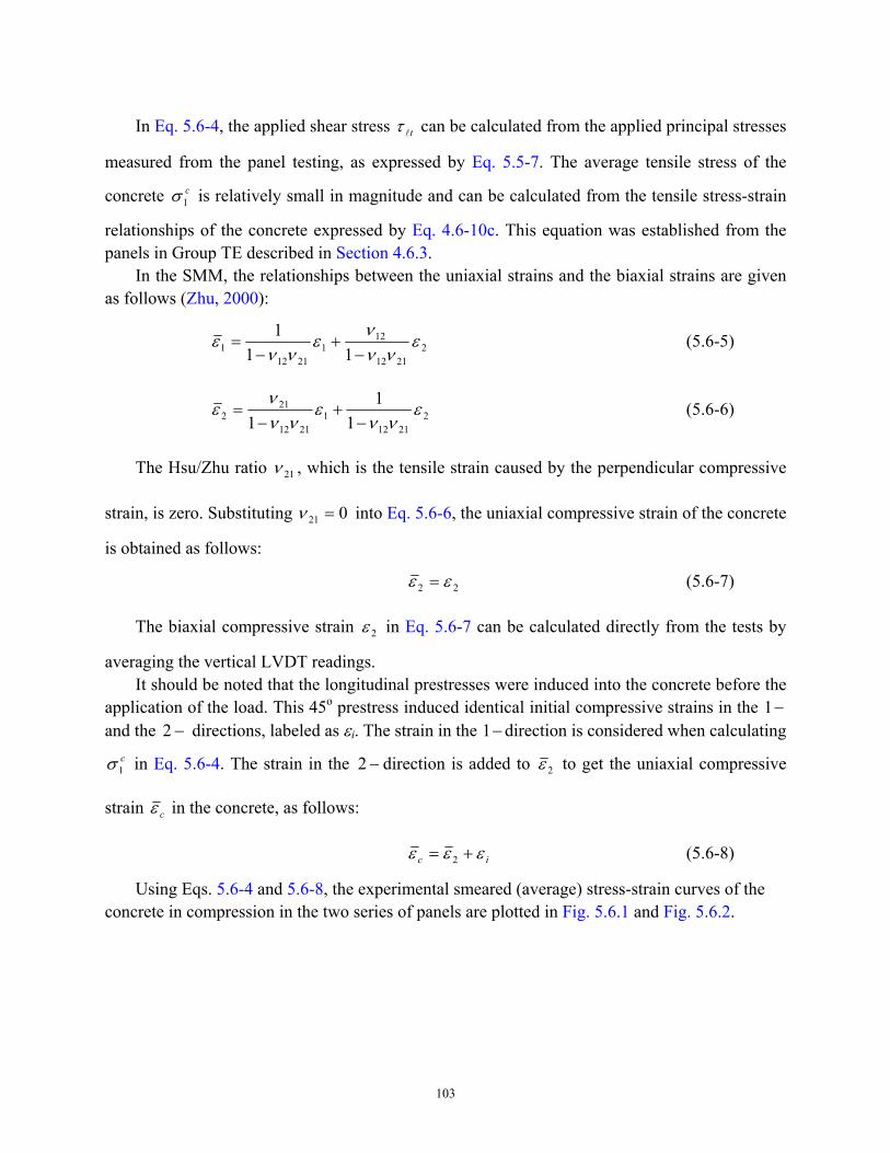
103

In Eq. 5.6-4, the applied shear stress tlτ can be calculated from the applied principal stresses

measured from the panel testing, as expressed by Eq. 5.5-7. The average tensile stress of the

concrete c1σ is relatively small in magnitude and can be calculated from the tensile stress-strain

relationships of the concrete expressed by Eq. 4.6-10c. This equation was established from the panels in Group TE described in Section 4.6.3.

In the SMM, the relationships between the uniaxial strains and the biaxial strains are given as follows (Zhu, 2000):

22112

121

21121 11

1 ενν

νε

ννε

−+

−= (5.6-5)

22112

12112

212 1

11

ενν

ενν

νε

−+

−= (5.6-6)

The Hsu/Zhu ratio 21ν , which is the tensile strain caused by the perpendicular compressive

strain, is zero. Substituting 021 =ν into Eq. 5.6-6, the uniaxial compressive strain of the concrete

is obtained as follows:

22 εε = (5.6-7)

The biaxial compressive strain 2ε in Eq. 5.6-7 can be calculated directly from the tests by

averaging the vertical LVDT readings. It should be noted that the longitudinal prestresses were induced into the concrete before the

application of the load. This 45o prestress induced identical initial compressive strains in the −1 and the −2 directions, labeled as εi. The strain in the −1 direction is considered when calculating

c1σ in Eq. 5.6-4. The strain in the −2 direction is added to 2ε to get the uniaxial compressive

strain cε in the concrete, as follows:

ic εεε += 2 (5.6-8)

Using Eqs. 5.6-4 and 5.6-8, the experimental smeared (average) stress-strain curves of the concrete in compression in the two series of panels are plotted in Fig. 5.6.1 and Fig. 5.6.2.

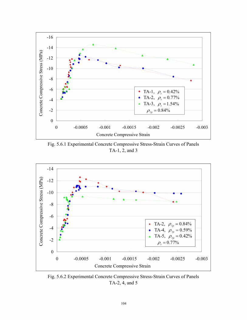
104

-14

-12

-10

-8

-6

-4

-2

0-0.003-0.0025-0.002-0.0015-0.001-0.00050

Concrete Compressive Strain

Con

cret

e C

ompr

essi

ve S

tress

(MPa

)

TA-2TA-4TA-5

Fig. 5.6.2 Experimental Concrete Compressive Stress-Strain Curves of Panels TA-2, 4, and 5


%77.0=tρ


%77.0=tρ

-16

-14

-12

-10

-8

-6

-4

-2

0-0.003-0.0025-0.002-0.0015-0.001-0.00050


Con

cret

e C

ompr

essi

ve S

tress

(MPa

)

TA-1TA-2TA-3

Fig. 5.6.1 Experimental Concrete Compressive Stress-Strain Curves of Panels TA-1, 2, and 3

TA-1, %42.0=tρ TA-2, %77.0=tρ TA-3, %54.1=tρ

%84.0=plρ

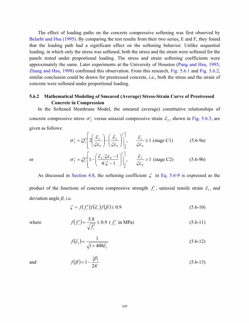
105

The effect of loading paths on the concrete compressive softening was first observed by Belarbi and Hsu (1995). By comparing the test results from their two series, E and F, they found that the loading path had a significant effect on the softening behavior. Unlike sequential loading, in which only the stress was softened, both the stress and the strain were softened for the panels tested under proportional loading. The stress and strain softening coefficients were approximately the same. Later experiments at the University of Houston (Pang and Hsu, 1995; Zhang and Hsu, 1998) confirmed this observation. From this research, Fig. 5.6.1 and Fig. 5.6.2, similar conclusion could be drawn for prestressed concrete, i.e., both the stress and the strain of concrete were softened under proportional loading.

5.6.2 Mathematical Modeling of Smeared (Average) Stress-Strain Curve of Prestressed

Concrete in Compression In the Softened Membrane Model, the smeared (average) constitutive relationships of

concrete compressive stress c2σ versus uniaxial compressive strain 2ε , shown in Fig. 5.6.3, are

given as follows:

−

′=

2

0

2

0

22 2

ζεε

ζεε

ζσ cc f , 1

0

2 ≤ζεε (stage C1) (5.6-9a)

or

−−

−′=2

022 14

11

ζζεε

ζσ cc f , 1

0

2 >ζεε (stage C2) (5.6-9b)

As discussed in Section 4.8, the softening coefficient ζ in Eq. 5.6-9 is expressed as the

product of the functions of concrete compressive strength cf ′ , uniaxial tensile strain 1ε , and

deviation angle β, i.e.

( ) ( ) ( ) 9.01 ≤′= βεζ ffff c (5.6-10)

where ( ) 9.08.5≤

′=′

cc f

ff ( cf ′ in MPa) (5.6-11)

( )1

1 40011

εε

+=f (5.6-12)

and ( )o24

1β

β −=f (5.6-13)

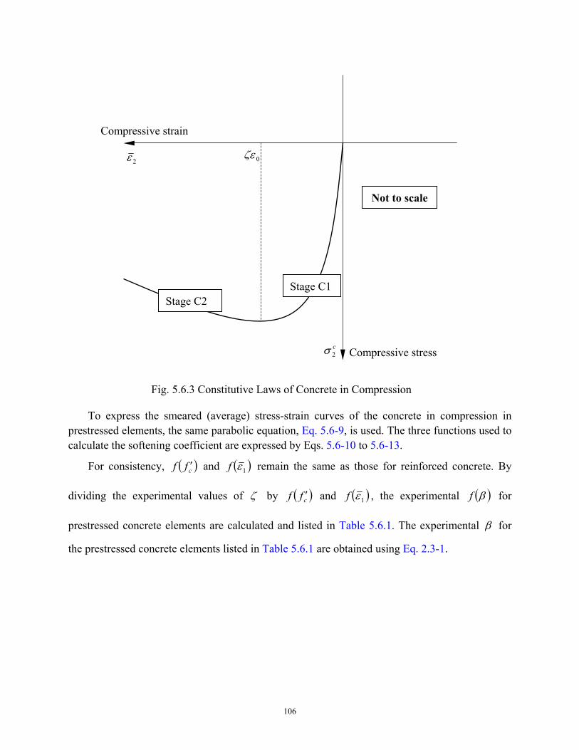
106

To express the smeared (average) stress-strain curves of the concrete in compression in

prestressed elements, the same parabolic equation, Eq. 5.6-9, is used. The three functions used to calculate the softening coefficient are expressed by Eqs. 5.6-10 to 5.6-13.

For consistency, ( )cff ′ and ( )1εf remain the same as those for reinforced concrete. By

dividing the experimental values of ζ by ( )cff ′ and ( )1εf , the experimental ( )βf for

prestressed concrete elements are calculated and listed in Table 5.6.1. The experimental β for

the prestressed concrete elements listed in Table 5.6.1 are obtained using Eq. 2.3-1.

2ε

c2σ

0ζε

Stage C1Stage C2

Compressive strain

Compressive stress

Not to scale

Fig. 5.6.3 Constitutive Laws of Concrete in Compression

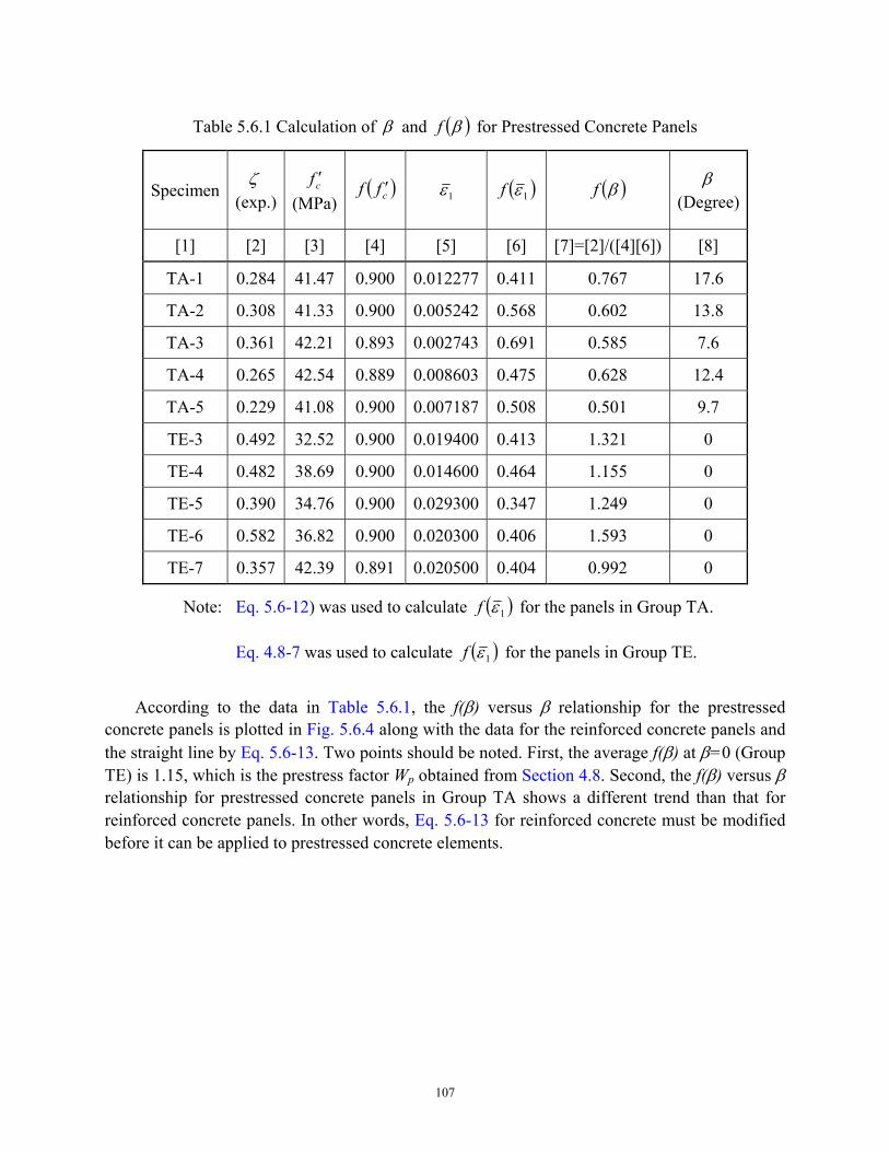
107

According to the data in Table 5.6.1, the f(β) versus β relationship for the prestressed concrete panels is plotted in Fig. 5.6.4 along with the data for the reinforced concrete panels and the straight line by Eq. 5.6-13. Two points should be noted. First, the average f(β) at β=0 (Group TE) is 1.15, which is the prestress factor Wp obtained from Section 4.8. Second, the f(β) versus β relationship for prestressed concrete panels in Group TA shows a different trend than that for reinforced concrete panels. In other words, Eq. 5.6-13 for reinforced concrete must be modified before it can be applied to prestressed concrete elements.

Table 5.6.1 Calculation of β and ( )βf for Prestressed Concrete Panels

Specimen ζ

(exp.) cf ′

(MPa) ( )cff ′ 1ε ( )1εf ( )βf β

(Degree)

[1] [2] [3] [4] [5] [6] [7]=[2]/([4][6]) [8]

TA-1 0.284 41.47 0.900 0.012277 0.411 0.767 17.6

TA-2 0.308 41.33 0.900 0.005242 0.568 0.602 13.8

TA-3 0.361 42.21 0.893 0.002743 0.691 0.585 7.6

TA-4 0.265 42.54 0.889 0.008603 0.475 0.628 12.4

TA-5 0.229 41.08 0.900 0.007187 0.508 0.501 9.7

TE-3 0.492 32.52 0.900 0.019400 0.413 1.321 0

TE-4 0.482 38.69 0.900 0.014600 0.464 1.155 0

TE-5 0.390 34.76 0.900 0.029300 0.347 1.249 0

TE-6 0.582 36.82 0.900 0.020300 0.406 1.593 0

TE-7 0.357 42.39 0.891 0.020500 0.404 0.992 0

Note: Eq. 5.6-12) was used to calculate ( )1εf for the panels in Group TA.

Eq. 4.8-7 was used to calculate ( )1εf for the panels in Group TE.

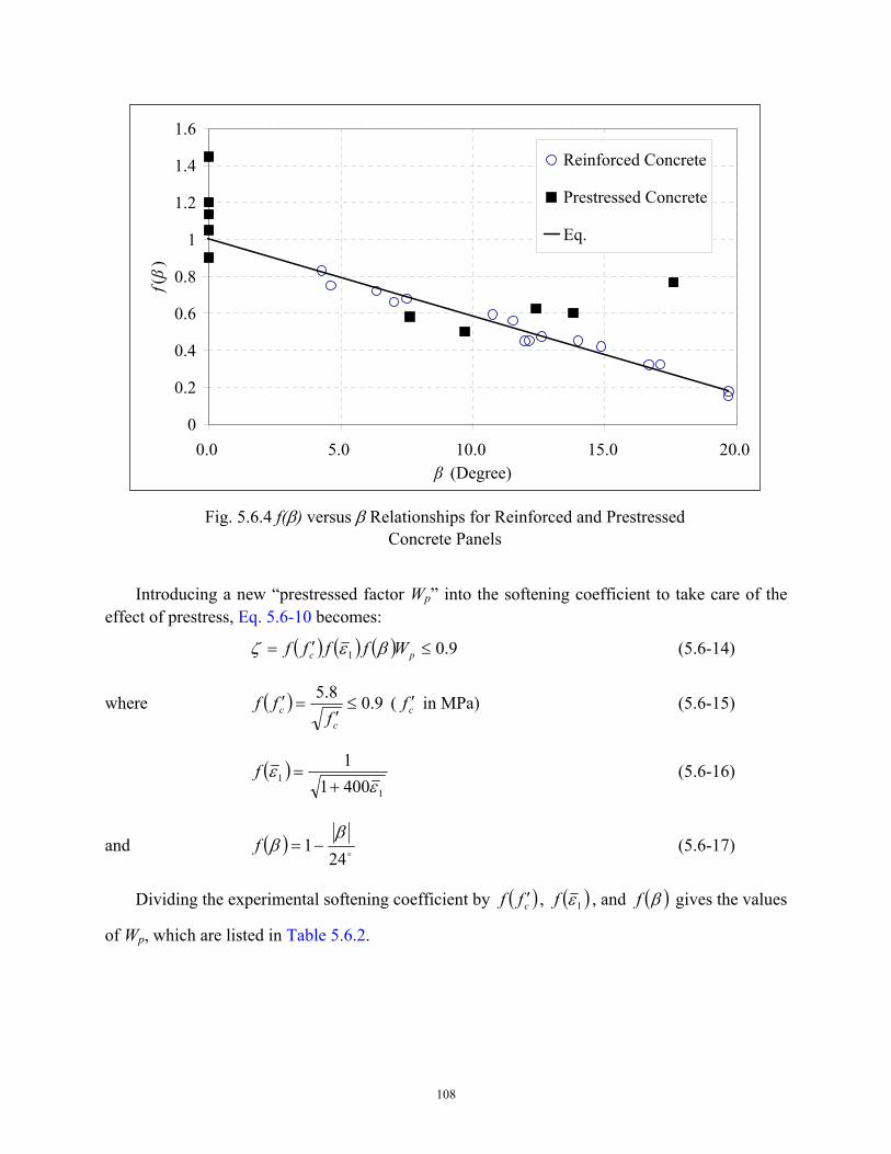
108

Introducing a new “prestressed factor Wp” into the softening coefficient to take care of the

effect of prestress, Eq. 5.6-10 becomes:

( ) ( ) ( ) 9.01 ≤′= pc Wffff βεζ (5.6-14)

where ( ) 9.08.5≤

′=′

cc f

ff ( cf ′ in MPa) (5.6-15)

( )1

1 40011

εε

+=f (5.6-16)

and ( )o24

1β

β −=f (5.6-17)

Dividing the experimental softening coefficient by ( )cff ′ , ( )1εf , and ( )βf gives the values

of Wp, which are listed in Table 5.6.2.

Fig. 5.6.4 f(β) versus β Relationships for Reinforced and Prestressed Concrete Panels

0

0.2

0.4

0.6

0.8

1

1.2

1.4

1.6

0.0 5.0 10.0 15.0 20.0β (Degree)

f(β

)Reinforced Concrete

Prestressed Concrete

Eq. (7-21)

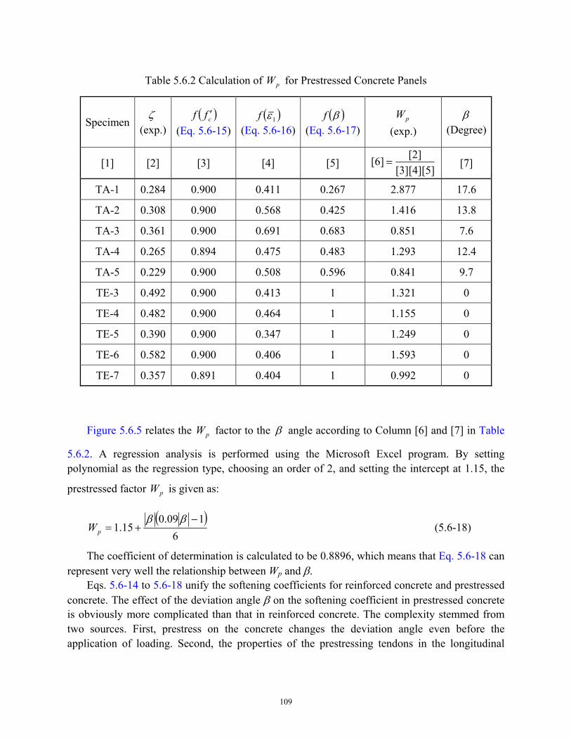
109

Figure 5.6.5 relates the pW factor to the β angle according to Column [6] and [7] in Table

5.6.2. A regression analysis is performed using the Microsoft Excel program. By setting polynomial as the regression type, choosing an order of 2, and setting the intercept at 1.15, the

prestressed factor pW is given as:

( )

6109.0

15.1−

+=ββ

pW (5.6-18)

The coefficient of determination is calculated to be 0.8896, which means that Eq. 5.6-18 can represent very well the relationship between Wp and β.

Eqs. 5.6-14 to 5.6-18 unify the softening coefficients for reinforced concrete and prestressed concrete. The effect of the deviation angle β on the softening coefficient in prestressed concrete is obviously more complicated than that in reinforced concrete. The complexity stemmed from two sources. First, prestress on the concrete changes the deviation angle even before the application of loading. Second, the properties of the prestressing tendons in the longitudinal

Table 5.6.2 Calculation of pW for Prestressed Concrete Panels

Specimen ζ

(exp.) ( )cff ′

(Eq. 5.6-15)( )1εf

(Eq. 5.6-16)( )βf

(Eq. 5.6-17)pW

(exp.) β

(Degree)

[1] [2] [3] [4] [5] [3][4][5][2][6] = [7]

TA-1 0.284 0.900 0.411 0.267 2.877 17.6

TA-2 0.308 0.900 0.568 0.425 1.416 13.8

TA-3 0.361 0.900 0.691 0.683 0.851 7.6

TA-4 0.265 0.894 0.475 0.483 1.293 12.4

TA-5 0.229 0.900 0.508 0.596 0.841 9.7

TE-3 0.492 0.900 0.413 1 1.321 0

TE-4 0.482 0.900 0.464 1 1.155 0

TE-5 0.390 0.900 0.347 1 1.249 0

TE-6 0.582 0.900 0.406 1 1.593 0

TE-7 0.357 0.891 0.404 1 0.992 0

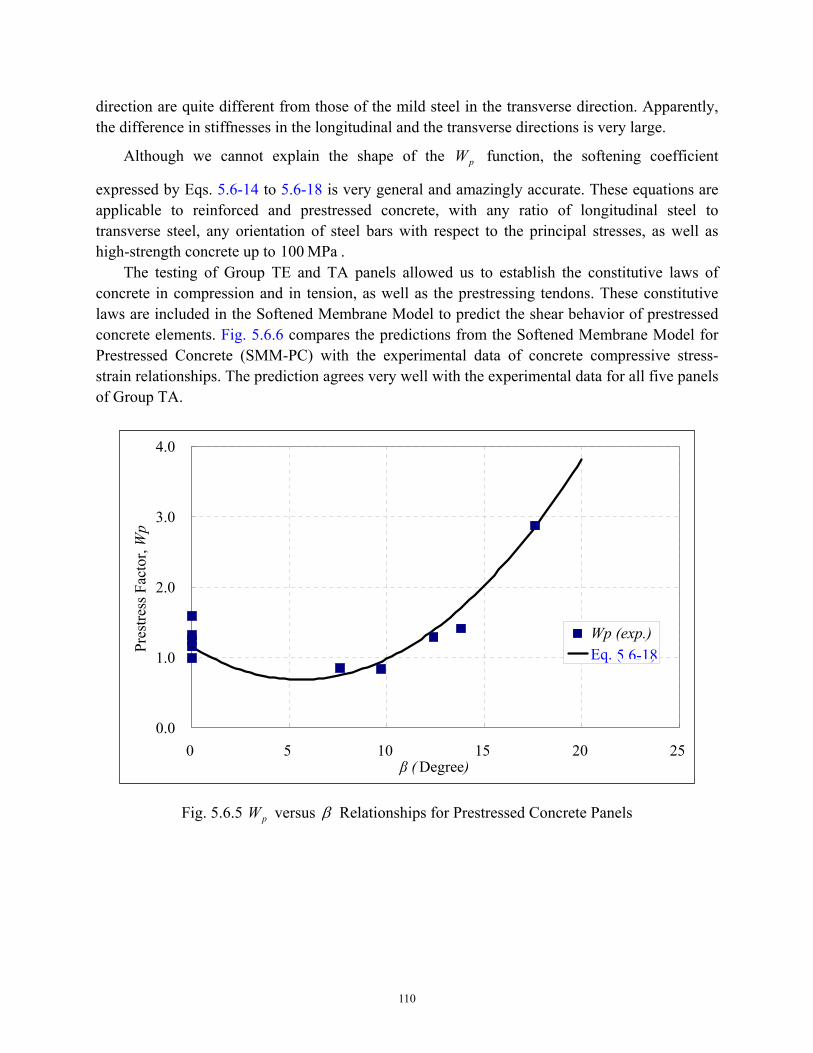
110

direction are quite different from those of the mild steel in the transverse direction. Apparently, the difference in stiffnesses in the longitudinal and the transverse directions is very large.

Although we cannot explain the shape of the pW function, the softening coefficient

expressed by Eqs. 5.6-14 to 5.6-18 is very general and amazingly accurate. These equations are applicable to reinforced and prestressed concrete, with any ratio of longitudinal steel to transverse steel, any orientation of steel bars with respect to the principal stresses, as well as high-strength concrete up to MPa 100 .

The testing of Group TE and TA panels allowed us to establish the constitutive laws of concrete in compression and in tension, as well as the prestressing tendons. These constitutive laws are included in the Softened Membrane Model to predict the shear behavior of prestressed concrete elements. Fig. 5.6.6 compares the predictions from the Softened Membrane Model for Prestressed Concrete (SMM-PC) with the experimental data of concrete compressive stress-strain relationships. The prediction agrees very well with the experimental data for all five panels of Group TA.

Fig. 5.6.5 pW versus β Relationships for Prestressed Concrete Panels

0.0

1.0

2.0

3.0

4.0

0 5 10 15 20 25β ( Degree)

Pres

tress

Fac

tor,

Wp

Wp (exp.)Eq. (7-27)5.6-18

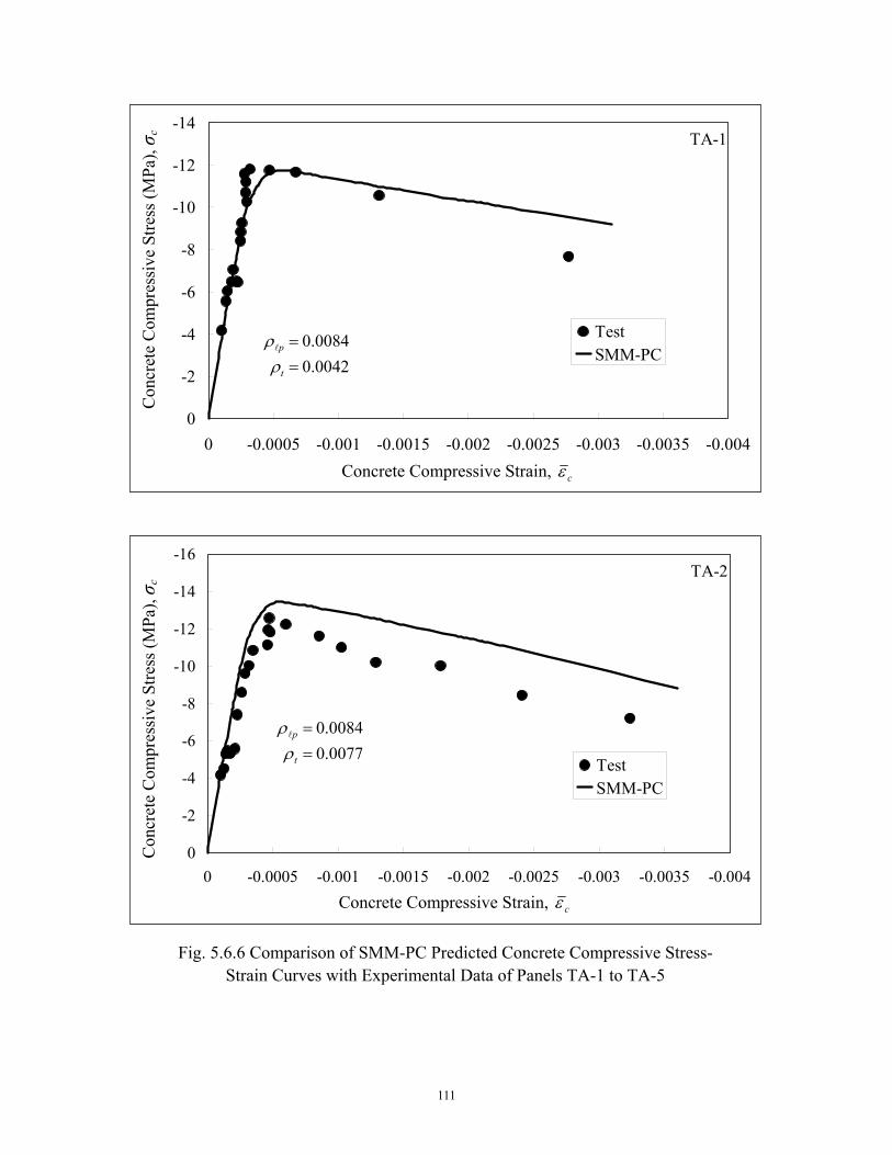
111

TA-2-16

-14

-12

-10

-8

-6

-4

-2

0-0.004-0.0035-0.003-0.0025-0.002-0.0015-0.001-0.00050


Con

cret

e C

ompr

essi

ve S

tress

(MPa

)

TestSMM-PC

TA-1-14

-12

-10

-8

-6

-4

-2

0-0.004-0.0035-0.003-0.0025-0.002-0.0015-0.001-0.00050


Con

cret

e C

ompr

essi

ve S

tress

(MPa

)

TestSMM-PC

Fig. 5.6.6 Comparison of SMM-PC Predicted Concrete Compressive Stress-Strain Curves with Experimental Data of Panels TA-1 to TA-5

Concrete Compressive Strain, cε

Con

cret

e C

ompr

essi

ve S

tress

(MPa

), σ c


Con

cret

e C

ompr

essi

ve S

tress

(MPa

), σ c

0042.00084.0

==

t

p

ρρl

0077.00084.0

==

t

p

ρρl

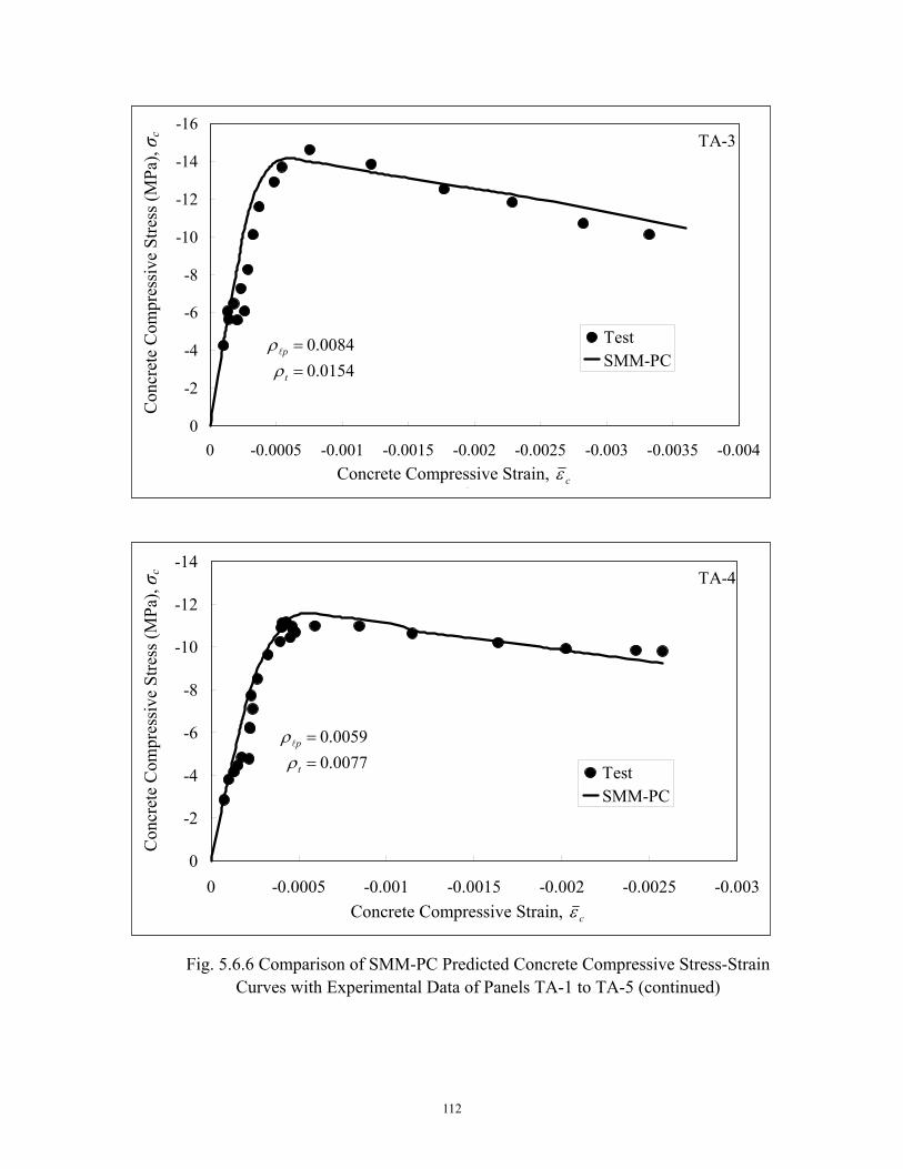
112

TA-4-14

-12

-10

-8

-6

-4

-2

0-0.003-0.0025-0.002-0.0015-0.001-0.00050


Con

cret

e C

ompr

essi

ve S

tress

(MPa

)

TestSMM-PC

TA-3-16

-14

-12

-10

-8

-6

-4

-2

0-0.004-0.0035-0.003-0.0025-0.002-0.0015-0.001-0.00050


Con

cret

e C

ompr

essi

ve S

tress

(MPa

)

TestSMM-PC

Fig. 5.6.6 Comparison of SMM-PC Predicted Concrete Compressive Stress-Strain Curves with Experimental Data of Panels TA-1 to TA-5 (continued)


Con

cret

e C

ompr

essi

ve S

tress

(MPa

), σ c


Con

cret

e C

ompr

essi

ve S

tress

(MPa

), σ c

0154.00084.0

==

t

p

ρρl

0077.00059.0

==

t

p

ρρl

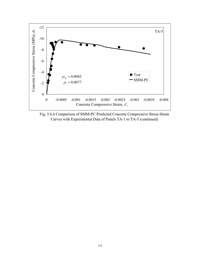
113

TA-5-12

-10

-8

-6

-4

-2

0-0.004-0.0035-0.003-0.0025-0.002-0.0015-0.001-0.00050


Con

cret

e C

ompr

essi

ve S

tress

(MPa

)

TestSMM-PC

Fig. 5.6.6 Comparison of SMM-PC Predicted Concrete Compressive Stress-Strain Curves with Experimental Data of Panels TA-1 to TA-5 (continued)


Con

cret

e C

ompr

essi

ve S

tress

(MPa

), σ c

0077.00042.0

==

t

p

ρρl

115

CHAPTER 6

ANALYTICAL MODELS OF PRESTRESSED CONCRETE PANELS

6.1 Introduction Reinforced concrete structures can be visualized as assemblies of membrane elements, and

their behavior can be predicted using the finite element method once the constitutive relationships of the elements are established. At the University of Houston, Zhong (2005) developed a nonlinear finite element program, named Simulation of Reinforced Concrete Structures (SRCS), for analysis of reinforced concrete structures. In SRCS, based on the Cyclic Softened Membrane Model (CSMM) (Mansour, 2001; Mansour and Hsu, 2005a and 2005b), a two-dimensional reinforced concrete plane stress material module and three uniaxial material modules of steel and concrete were developed and implemented into the object-oriented finite element framework OpenSees (Fenves 2001). SRCS is proven to successfully predict the behavior of reinforced concrete plane stress structures subjected to static, reversed cyclic, and dynamic loading.

In the present research project, the Softened Membrane Model for Prestressed Concrete (SMM-PC) has been developed to predict the response of prestressed concrete membrane elements under shear loading. Therefore, a new finite element program for prestressed concrete structures can be developed based on SRCS. The key to this program are the following two points: (1) new constitutive relationships of prestressing tendons embedded in concrete; and (2) revised constitutive relationships of concrete considering the effect of prestress. These new constitutive relationships of materials need to be implemented into SRCS based on the OpenSees framework.

This chapter summarizes the equations of equilibrium, compatibility, and constitutive relationships used in the Softened Membrane Model for Prestressed Concrete (SMM-PC). Both the constitutive laws and the analytical model presented in Chapters 4 through 6 will be applied to prestressed concrete beams. Basically, tests on prestressed concrete beams are performed, and an analytical model for the shear behavior of prestressed concrete beams is developed.

The three equilibrium equations and three compatibility equations are summarized in Section 6.2.1; the relationships between the biaxial strains and the uniaxial strains are given in Section 6.2.2; and the constitutive laws of the materials are presented in Section 6.2.3 and Section 6.2.4. The algorithm to solve all the equations is shown in Section 6.2.5. The analytical results of panels in Group TA are presented in Section 6.3 and compared with the test results.

6.2 Fundamentals of Softened Membrane Model for Prestressed Concrete Fig. 6.2.1(a) shows a prestressed concrete element subjected to in-plane stresses. As with the

SMM, two reference Cartesian coordinates are used in the SMM-PC, as shown in Fig. 6.2.1(e). The first reference Cartesian t−l coordinate system represents the directions of the longitudinal and transverse reinforcements. The second reference Cartesian 21− coordinate system

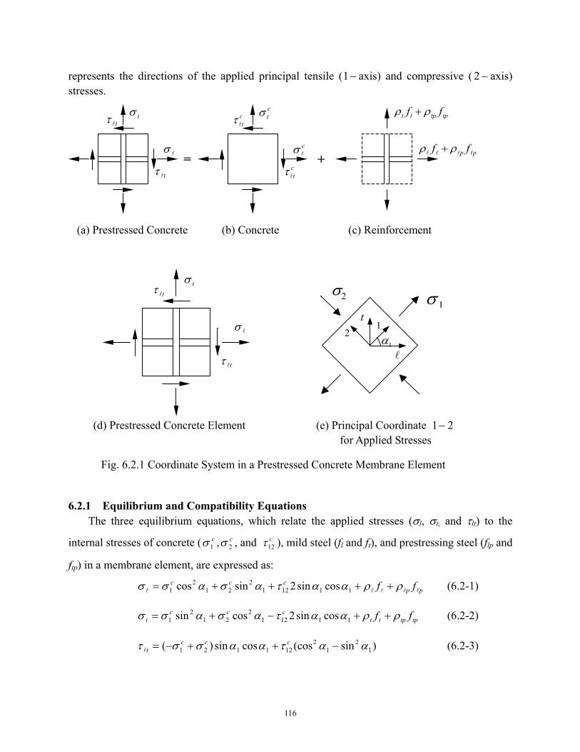
116

represents the directions of the applied principal tensile ( −1 axis) and compressive ( −2 axis) stresses.

6.2.1 Equilibrium and Compatibility Equations

The three equilibrium equations, which relate the applied stresses (σl, σt, and τlt) to the

internal stresses of concrete ( c1σ , c

2σ , and c12τ ), mild steel (fl and ft), and prestressing steel (flp and

ftp) in a membrane element, are expressed as:

ppccc ff lllll ρραατασασσ ++++= 11121

221


tptpttccc

t ff ρραατασασσ ++−+= 111212

212


)sin(coscossin)( 12

12

121121 ααταασστ −++−= ccctl (6.2-3)

clσlσ

Fig. 6.2.1 Coordinate System in a Prestressed Concrete Membrane Element

(d) Prestressed Concrete Element (e) Principal Coordinate 21− for Applied Stresses

=tlτ

tσtlτ

ctσ

ctlτ

ctlτ

tptptt ff ρρ +

pp ff llll ρρ ++

lσ

tlτ

tσ tlτ

(a) Prestressed Concrete (b) Concrete (c) Reinforcement

2σ 1σ

21

l

t

1α

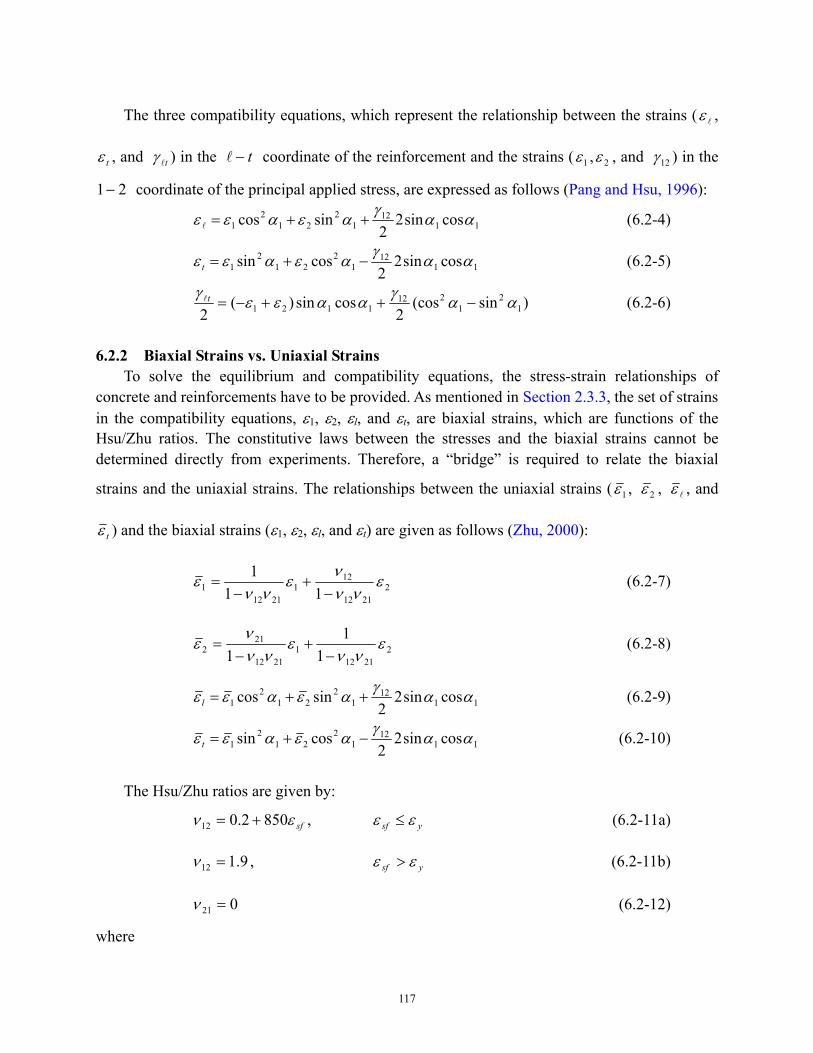
117

The three compatibility equations, which represent the relationship between the strains ( lε ,

tε , and tlγ ) in the t−l coordinate of the reinforcement and the strains ( 1ε , 2ε , and 12γ ) in the

21− coordinate of the principal applied stress, are expressed as follows (Pang and Hsu, 1996):

1112

12

212

1 cossin22

sincos ααγαεαεε ++=l (6.2-4)

1112

12

212

1 cossin22

cossin ααγαεαεε −+=t (6.2-5)

)sin(cos2

cossin)(2 1

21

2121121 ααγααεεγ

−++−=tl (6.2-6)

6.2.2 Biaxial Strains vs. Uniaxial Strains

To solve the equilibrium and compatibility equations, the stress-strain relationships of concrete and reinforcements have to be provided. As mentioned in Section 2.3.3, the set of strains in the compatibility equations, ε1, ε2, εl, and εt, are biaxial strains, which are functions of the Hsu/Zhu ratios. The constitutive laws between the stresses and the biaxial strains cannot be determined directly from experiments. Therefore, a “bridge” is required to relate the biaxial

strains and the uniaxial strains. The relationships between the uniaxial strains ( 1ε , 2ε , lε , and

tε ) and the biaxial strains (ε1, ε2, εl, and εt) are given as follows (Zhu, 2000):

22112

121

21121 11

1 ενν

νε

ννε

−+

−= (6.2-7)

22112

12112

212 1

11

ενν

ενν

νε

−+

−= (6.2-8)

1112

12

212

1 cossin22

sincos ααγαεαεε ++=l (6.2-9)

1112

12

212

1 cossin22

cossin ααγαεαεε −+=t (6.2-10)

The Hsu/Zhu ratios are given by:

sfεν 8502.012 += , ysf εε ≤ (6.2-11a)

9.112 =ν , ysf εε > (6.2-11b)

021 =ν (6.2-12)

where

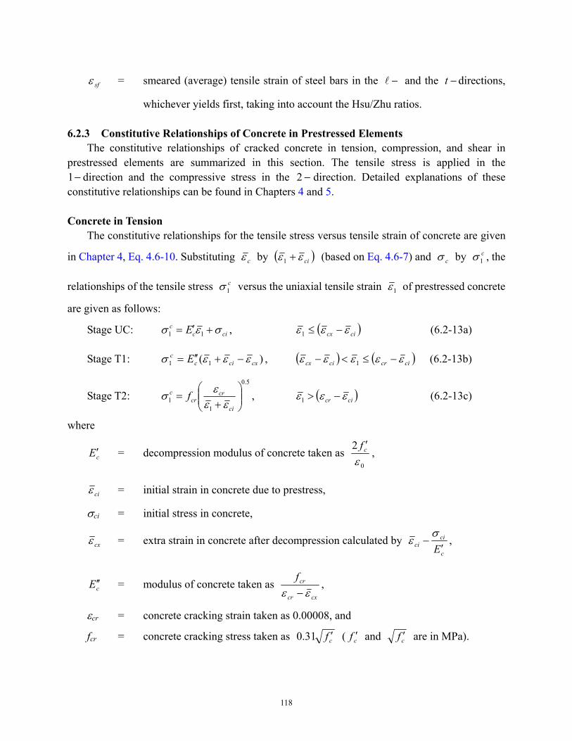
118

sfε = smeared (average) tensile strain of steel bars in the −l and the −t directions,

whichever yields first, taking into account the Hsu/Zhu ratios.

6.2.3 Constitutive Relationships of Concrete in Prestressed Elements The constitutive relationships of cracked concrete in tension, compression, and shear in

prestressed elements are summarized in this section. The tensile stress is applied in the −1 direction and the compressive stress in the −2 direction. Detailed explanations of these

constitutive relationships can be found in Chapters 4 and 5.

Concrete in Tension The constitutive relationships for the tensile stress versus tensile strain of concrete are given

in Chapter 4, Eq. 4.6-10. Substituting cε by ( )ciεε +1 (based on Eq. 4.6-7) and cσ by c1σ , the

relationships of the tensile stress c1σ versus the uniaxial tensile strain 1ε of prestressed concrete

are given as follows:

Stage UC: cicc E σεσ +′= 11 , ( )cicx εεε −≤1 (6.2-13a)

Stage T1: )( 11 cxcicc E εεεσ −+′′= , ( ) ( )cicrcicx εεεεε −≤<− 1 (6.2-13b)

Stage T2: 5.0

11

+

=ci

crcr

c fεε

εσ , ( )cicr εεε −>1 (6.2-13c)

where

cE ′ = decompression modulus of concrete taken as 0

2εcf ′ ,

ciε = initial strain in concrete due to prestress,

σci = initial stress in concrete,

cxε = extra strain in concrete after decompression calculated by c

cici E ′−σ

ε ,

cE ′′ = modulus of concrete taken as cxcr

crfεε −

,


fcr = concrete cracking stress taken as cf ′31.0 ( cf ′ and cf ′ are in MPa).

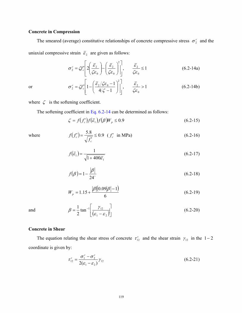
119

Concrete in Compression

The smeared (average) constitutive relationships of concrete compressive stress c2σ and the

uniaxial compressive strain 2ε are given as follows:

−

′=

2

0

2

0

22 2

ζεε

ζεε

ζσ cc f , 1

0

2 ≤ζεε (6.2-14a)

or

−−

−′=2

022 14

11

ζζεε

ζσ cc f , 1

0

2 >ζεε (6.2-14b)

where ζ is the softening coefficient.

The softening coefficient in Eq. 6.2-14 can be determined as follows:

( ) ( ) ( ) 9.01 ≤′= pc Wffff βεζ (6.2-15)

where ( ) 9.08.5≤

′=′

cc fff ( cf ′ in MPa) (6.2-16)

( )1

1 40011

εε

+=f (6.2-17)

( )o24

1β

β −=f (6.2-18)

( )

6109.0

15.1−

+=ββ

pW (6.2-19)

and ( )

−

= −

21

121tan21

εεγ

β (6.2-20)

Concrete in Shear

The equation relating the shear stress of concrete c12τ and the shear strain 12γ in the 21−

coordinate is given by:

1221

2112 )(2

γεεσστ−−

=cc

c (6.2-21)

120

6.2.4 Constitutive Relationships of Reinforcements Two types of reinforcements are embedded in concrete, prestressing tendons and mild steel

bars.

Prestressing Tendons Embedded in Concrete The smeared (average) stress-strain relationships of prestressing tendons embedded in

concrete are given as follows:

spsps Ef ε= , ps

pus E

f7.0<ε (6.2-22a)

or 51

5

1

′

′′+

′′=

pu

sps

spsps

fE

Ef

ε

ε,

ps

pus E

f7.0≥ε (6.2-22b)

where Eps = elastic modulus of prestressing tendons taken as GPa 200 ( ksi 29000 ), fpu = ultimate strength of prestressing tendons taken as MPa 1862 ( ksi 270 ),

psE ′′ = modulus of prestressing tendons, used in plastic region (Eq. 6.2-22b), taken as

GPa 209 ( ksi 30345 ), and

puf ′ = revised strength of prestressing tendons taken as MPa 1793 ( ksi 260 ).

In the above equations, lp replaces ps in the subscript of symbols for the longitudinal tendons, and tp replaces ps for the transverse tendons.

Mild Steel Embedded in Concrete

The smeared (average) tensile stress-strain relationships of mild steel embedded in concrete in the t−l coordinate are the same in SMM. They can be expressed as follows:

Stage 1: sss Ef ε= , ns εε ≤ (6.2-23a)

Stage 2:

++−=

y

sys BBff

εε

)25.002.0()291.0( , ns εε > (6.2-23b)

Stage 3 (unloading): )( spsps Eff εε −−= , ps εε < (6.2-23c)

where )293.0( Byn −= εε (6.2-24)

and 5.1

1

=

y

cr

ff

Bρ

(6.2-25)

121

In the above equations, l replaces s in the subscript of symbols for the longitudinal steel, and t replaces s for the transverse steel.

6.2.5 Solution Algorithm

The solution procedure for the SMM-PC is given in the flow chart of Fig. 6.2.2. Similar to the SMM, two equilibrium equations, Eqs. 6.2-26 and 6.2-27, are also used to make the solution procedure more efficient. Eqs. 6.2-26 and 6.2-27 are derived from Eqs. 6.2-1 and 6.2-2:

)()( 21cc

ttptpttpp ffff σσσσρρρρ +−+=+++ lllll (6.2-26)

112121 2sin22cos)()( ατασσσσρρρρ cccttptpttpp ffff −−−−=−−+ lllll (6.2-27)

Defining pp fff lllll ρρρ +=][ and tptpttt fff ρρρ +=][ , the above two equations become:

)()(][][ 21cc

ttff σσσσρρ +−+=+ ll (6.2-28)

112121 2sin22cos)()(][][ ατασσσσρρ cccttff −−−−=− ll (6.2-29)

The solution procedure can also be described as follows (Fig. 6.2.2):

Step 1: Select a value of strain in the −2 direction, 2ε .

Step 2: Assume a value of shear strain in the 21− coordinate, γ12. Step 3: Assume a value of strain in the −1 direction, ε1. Step 4: Calculate steel strains εl, εt, and ν12, from Eqs. 6.2-4, 6.2-5, and 6.2-11,

respectively. Hsu/Zhu ratio ν21 is taken as zero.

Step 5: Calculate uniaxial strains 1ε , 2ε , lε , and tε from Eqs. 6.2-7 to 6.2-10.

Step 6: Calculate the concrete stresses c1σ , c

2σ and c12τ from Eqs. 6.2-13, 6.2-14, and

6.2-21, respectively. Step 7: Calculate the reinforcement stresses fl, ft, flp, and ftp from Eqs. 6.2-22 and 6.2-23.

Step 8: Calculate 1)][]([ tff ρρ +l and 1)][]([ tff ρρ −l .

Step 9: Calculate 2)][]([ tff ρρ +l and 2)][]([ tff ρρ −l , from Eqs. 6.2-28 and 6.2-29,

respectively.

Step 10: Compare 1)][]([ tff ρρ +l with 2)][]([ tff ρρ +l . When 2)][]([ tff ρρ +l is

larger than 1)][]([ tff ρρ +l , increase the tensile strain 1ε . Otherwise, decrease

122

1ε . Repeat steps 3 to 10 until 1)][]([ tff ρρ +l and 2)][]([ tff ρρ +l are close

enough within the specified accuracy.

Step 11: Compare 1)][]([ tff ρρ −l with 2)][]([ tff ρρ −l . When 2)][]([ tff ρρ −l is

larger than 1)][]([ tff ρρ −l , increase the value of shear strain 12γ . Otherwise,

decrease the shear strain 12γ . Repeat steps 2 to 11 until 1)][]([ tff ρρ −l and

2)][]([ tff ρρ −l are close enough within the specified accuracy.

Step 12: Calculate the applied shear stress tlτ and the corresponding shear strain tlγ from

Eq. 6.2-3 and 6.2-6, respectively. This will provide one point on the tlτ versus

tlγ curve.

Step 13: Select another value of 2ε and repeat steps 2 to 12. Calculations for a series of

2ε values will provide the whole tlτ versus tlγ curve.

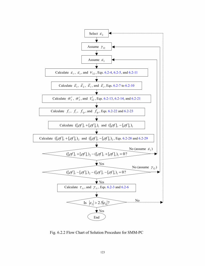
123

Select 2ε

Assume 12γ

Assume 1ε

Calculate lε , tε , and 12ν , Eqs. 6.2-4, 6.2-5, and 6.2-11

Calculate 1ε , 2ε , lε , and tε , Eqs. 6.2-7 to 6.2-10

Calculate c1σ , c

2σ , and c12τ , Eqs. 6.2-13, 6.2-14, and 6.2-21

Calculate lf , tf , pf l , and tpf , Eqs. 6.2-22 and 6.2-23

Calculate 1)][]([ tff ρρ +l and 1)][]([ tff ρρ −l

Calculate 2)][]([ tff ρρ +l and 2)][]([ tff ρρ −l , Eqs. 6.2-28 and 6.2-29

?0)][]([)][]([ 12 =+−+ tt ffff ρρρρ ll

?0)][]([)][]([ 12 =−−− tt ffff ρρρρ ll

Calculate tlτ , and tlγ , Eqs. 6.2-3 and 6.2-6

?5.2 Is 02 εε >

End

No (assume 1ε )

No (assume 12γ )

No

Yes

Yes

Yes

Fig. 6.2.2 Flow Chart of Solution Procedure for SMM-PC

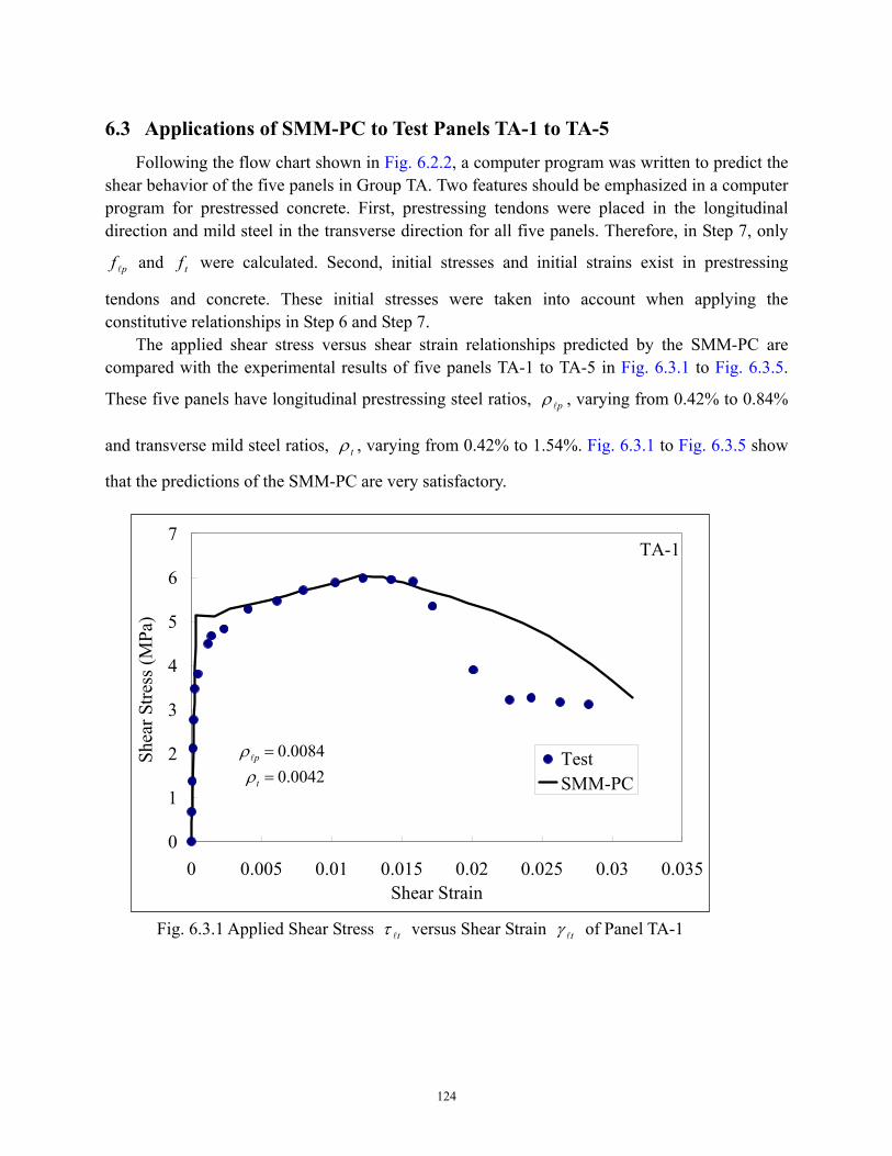
124

6.3 Applications of SMM-PC to Test Panels TA-1 to TA-5 Following the flow chart shown in Fig. 6.2.2, a computer program was written to predict the

shear behavior of the five panels in Group TA. Two features should be emphasized in a computer program for prestressed concrete. First, prestressing tendons were placed in the longitudinal direction and mild steel in the transverse direction for all five panels. Therefore, in Step 7, only

pf l and tf were calculated. Second, initial stresses and initial strains exist in prestressing

tendons and concrete. These initial stresses were taken into account when applying the constitutive relationships in Step 6 and Step 7.

The applied shear stress versus shear strain relationships predicted by the SMM-PC are compared with the experimental results of five panels TA-1 to TA-5 in Fig. 6.3.1 to Fig. 6.3.5.

These five panels have longitudinal prestressing steel ratios, plρ , varying from 0.42% to 0.84%

and transverse mild steel ratios, tρ , varying from 0.42% to 1.54%. Fig. 6.3.1 to Fig. 6.3.5 show

that the predictions of the SMM-PC are very satisfactory.

Fig. 6.3.1 Applied Shear Stress tlτ versus Shear Strain tlγ of Panel TA-1

TA-1

0

1

2

3

4

5

6

7

0 0.005 0.01 0.015 0.02 0.025 0.03 0.035Shear Strain

Shea

r Stre

ss (MPa

)

TestSMM-PC0042.0

0084.0==

t

p

ρρlSh

ear S

tress

(MPa

)

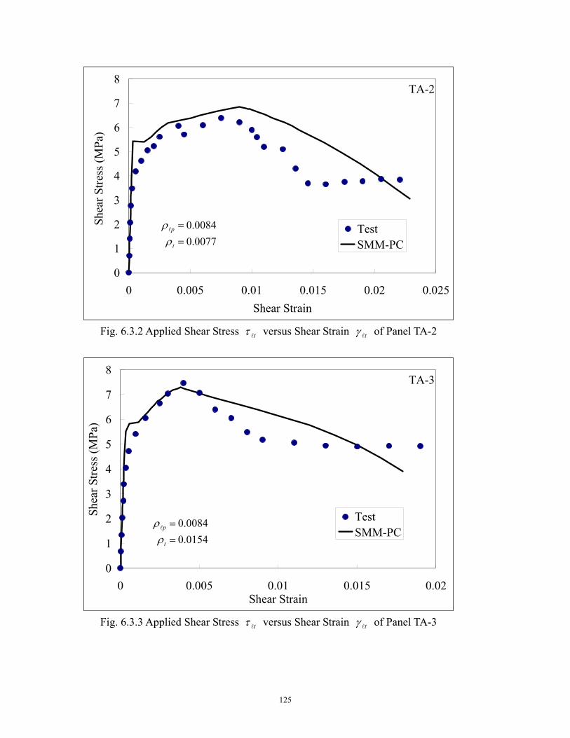
125


TA-3

0

1

2

3

4

5

6

7

8

0 0.005 0.01 0.015 0.02Shear Strain

Shea

r Stre

ss (MPa

)

TestSMM-PC0154.0

0084.0==

t

p

ρρl

Shea

r Stre

ss (M

Pa)


TA-2

0

1

2

3

4

5

6

7

8

0 0.005 0.01 0.015 0.02 0.025Shear Strain

Shea

r Stre

ss (MPa

)

TestSMM-PC0077.0

0084.0==

t

p

ρρl

Shea

r Stre

ss (M

Pa)

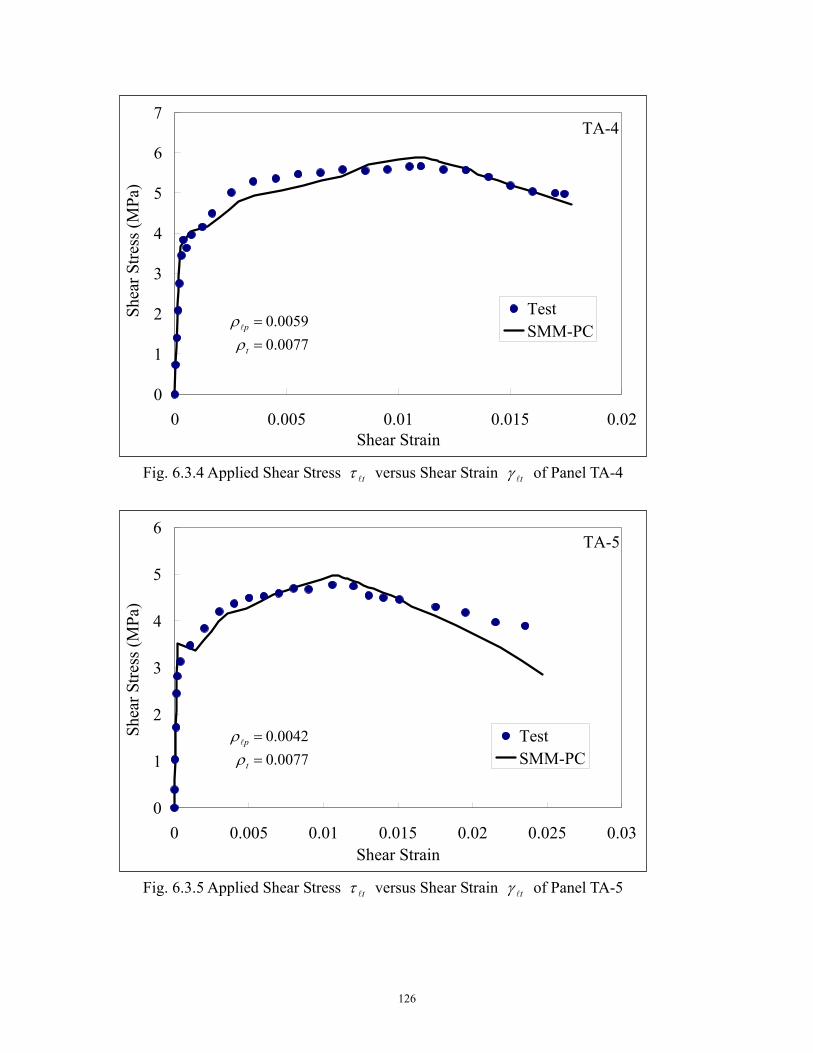
126


TA-4

0

1

2

3

4

5

6

7

0 0.005 0.01 0.015 0.02Shear Strain

Shea

r Stre

ss (MPa

)

TestSMM-PC

0077.00059.0

==

t

p

ρρl

Shea

r Stre

ss (M

Pa)


TA-5

0

1

2

3

4

5

6

0 0.005 0.01 0.015 0.02 0.025 0.03Shear Strain

Shea

r Stre

ss (MPa

)

TestSMM-PC0077.0

0042.0==

t

p

ρρl

Shea

r Stre

ss (M

Pa)

PART II

SHEAR IN PRESTRESSED CONCRETE BEAMS

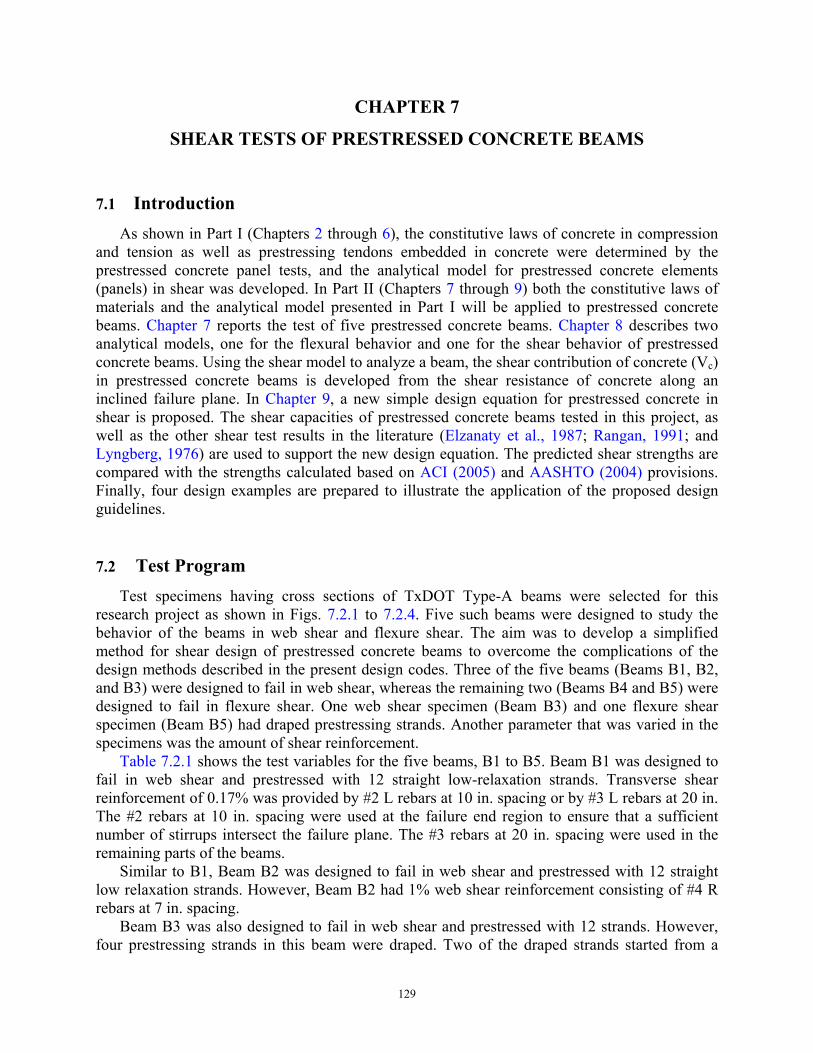
129

CHAPTER 7

SHEAR TESTS OF PRESTRESSED CONCRETE BEAMS

7.1 Introduction

As shown in Part I (Chapters 2 through 6), the constitutive laws of concrete in compression and tension as well as prestressing tendons embedded in concrete were determined by the prestressed concrete panel tests, and the analytical model for prestressed concrete elements (panels) in shear was developed. In Part II (Chapters 7 through 9) both the constitutive laws of materials and the analytical model presented in Part I will be applied to prestressed concrete beams. Chapter 7 reports the test of five prestressed concrete beams. Chapter 8 describes two analytical models, one for the flexural behavior and one for the shear behavior of prestressed concrete beams. Using the shear model to analyze a beam, the shear contribution of concrete (Vc) in prestressed concrete beams is developed from the shear resistance of concrete along an inclined failure plane. In Chapter 9, a new simple design equation for prestressed concrete in shear is proposed. The shear capacities of prestressed concrete beams tested in this project, as well as the other shear test results in the literature (Elzanaty et al., 1987; Rangan, 1991; and Lyngberg, 1976) are used to support the new design equation. The predicted shear strengths are compared with the strengths calculated based on ACI (2005) and AASHTO (2004) provisions. Finally, four design examples are prepared to illustrate the application of the proposed design guidelines.

7.2 Test Program

Test specimens having cross sections of TxDOT Type-A beams were selected for this research project as shown in Figs. 7.2.1 to 7.2.4. Five such beams were designed to study the behavior of the beams in web shear and flexure shear. The aim was to develop a simplified method for shear design of prestressed concrete beams to overcome the complications of the design methods described in the present design codes. Three of the five beams (Beams B1, B2, and B3) were designed to fail in web shear, whereas the remaining two (Beams B4 and B5) were designed to fail in flexure shear. One web shear specimen (Beam B3) and one flexure shear specimen (Beam B5) had draped prestressing strands. Another parameter that was varied in the specimens was the amount of shear reinforcement.

Table 7.2.1 shows the test variables for the five beams, B1 to B5. Beam B1 was designed to fail in web shear and prestressed with 12 straight low-relaxation strands. Transverse shear reinforcement of 0.17% was provided by #2 L rebars at 10 in. spacing or by #3 L rebars at 20 in. The #2 rebars at 10 in. spacing were used at the failure end region to ensure that a sufficient number of stirrups intersect the failure plane. The #3 rebars at 20 in. spacing were used in the remaining parts of the beams.

Similar to B1, Beam B2 was designed to fail in web shear and prestressed with 12 straight low relaxation strands. However, Beam B2 had 1% web shear reinforcement consisting of #4 R rebars at 7 in. spacing.

Beam B3 was also designed to fail in web shear and prestressed with 12 strands. However, four prestressing strands in this beam were draped. Two of the draped strands started from a

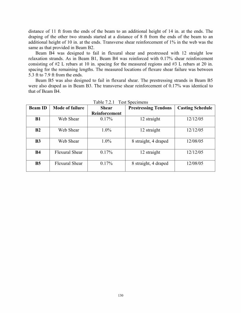
130

distance of 11 ft from the ends of the beam to an additional height of 14 in. at the ends. The draping of the other two strands started at a distance of 8 ft from the ends of the beam to an additional height of 10 in. at the ends. Transverse shear reinforcement of 1% in the web was the same as that provided in Beam B2.

Beam B4 was designed to fail in flexural shear and prestressed with 12 straight low relaxation strands. As in Beam B1, Beam B4 was reinforced with 0.17% shear reinforcement consisting of #2 L rebars at 10 in. spacing for the measured regions and #3 L rebars at 20 in. spacing for the remaining lengths. The measured locations of flexure shear failure was between 5.3 ft to 7.9 ft from the ends.

Beam B5 was also designed to fail in flexural shear. The prestressing strands in Beam B5 were also draped as in Beam B3. The transverse shear reinforcement of 0.17% was identical to that of Beam B4.

Table 7.2.1 Test Specimens

Beam ID Mode of failure Shear Reinforcement

Prestressing Tendons Casting Schedule

B1 Web Shear 0.17% 12 straight 12/12/05

B2 Web Shear 1.0% 12 straight 12/12/05

B3 Web Shear 1.0% 8 straight, 4 draped 12/08/05

B4 Flexural Shear 0.17% 12 straight 12/12/05

B5 Flexural Shear 0.17% 8 straight, 4 draped 12/08/05

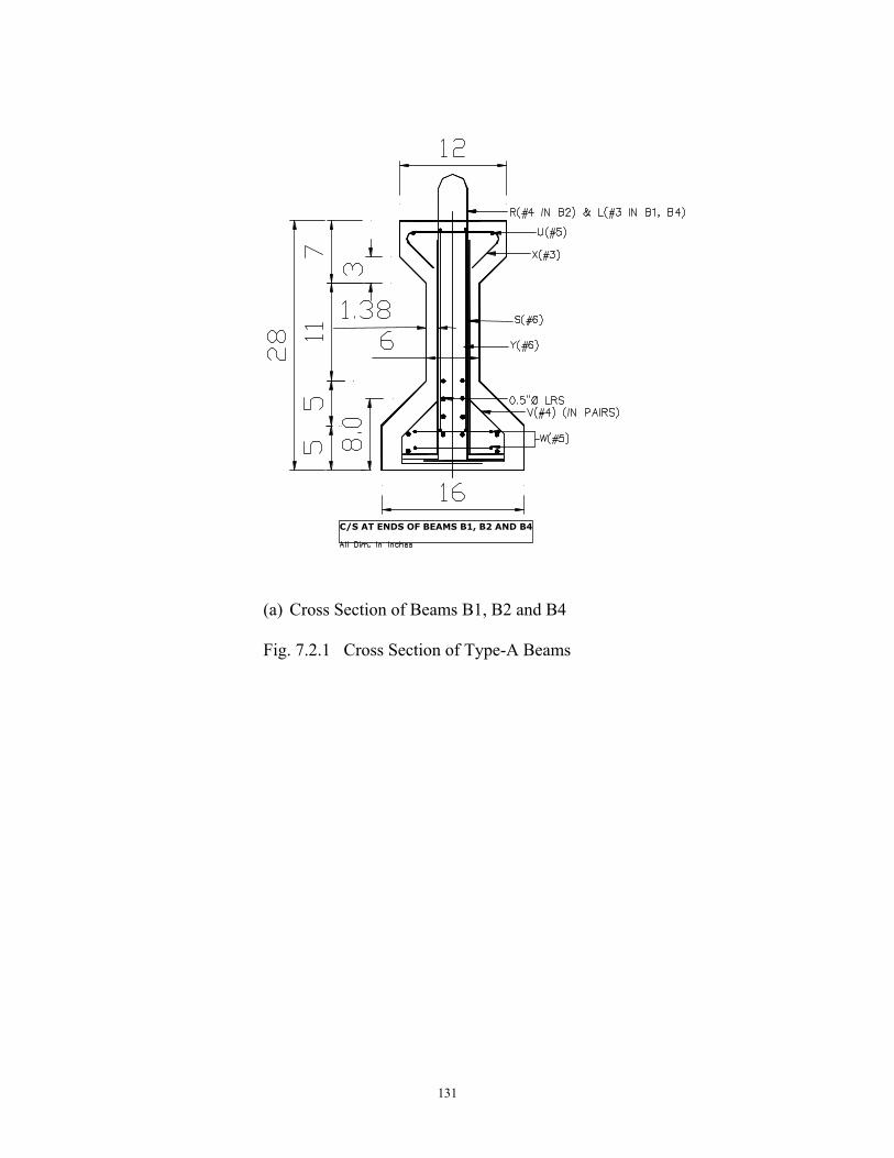
131

(a) Cross Section of Beams B1, B2 and B4 Fig. 7.2.1 Cross Section of Type-A Beams

C/S AT ENDS OF BEAMS B1, B2 AND B4

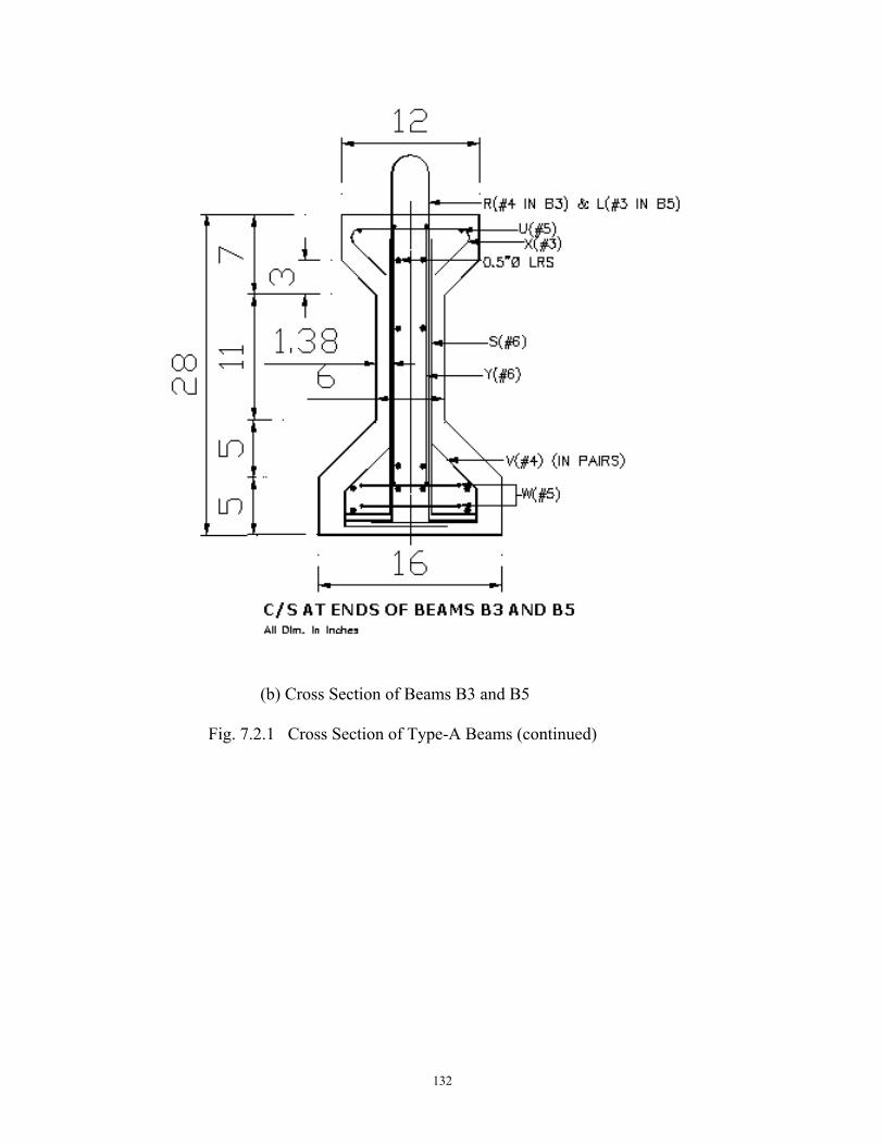
132

(b) Cross Section of Beams B3 and B5

Fig. 7.2.1 Cross Section of Type-A Beams (continued)

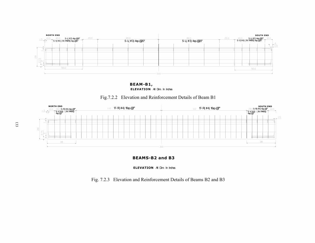
133

Fig.7.2.2 Elevation and Reinforcement Details of Beam B1

Fig. 7.2.3 Elevation and Reinforcement Details of Beams B2 and B3

NORTH END SOUTH END

5- L( #2) 4sp.@10" 5- L( #3) 4sp.@20"

BEAM-B1, ELEVATION All Dim. In Inches

5- L( #3) 4sp.@20" 5- L( #2) 4sp.@10"

5- V( #4) ( IN PAIRS) 4sp.@10" 5- V( #4) ( IN PAIRS) 4sp.@10"

NORTH END SOUTH END5- R( #4) 4sp.@7" 17- R( #4) 16sp.@7"

BEAMS-B2 and B3 ELEVATION All Dim. In Inches

17- R( #4) 16sp.@7" 5- R( #4) 4sp.@7" 5- V( #4) ( IN PAIRS)4sp.@7"

5- V( #4) ( IN PAIRS)4sp.@7"

133

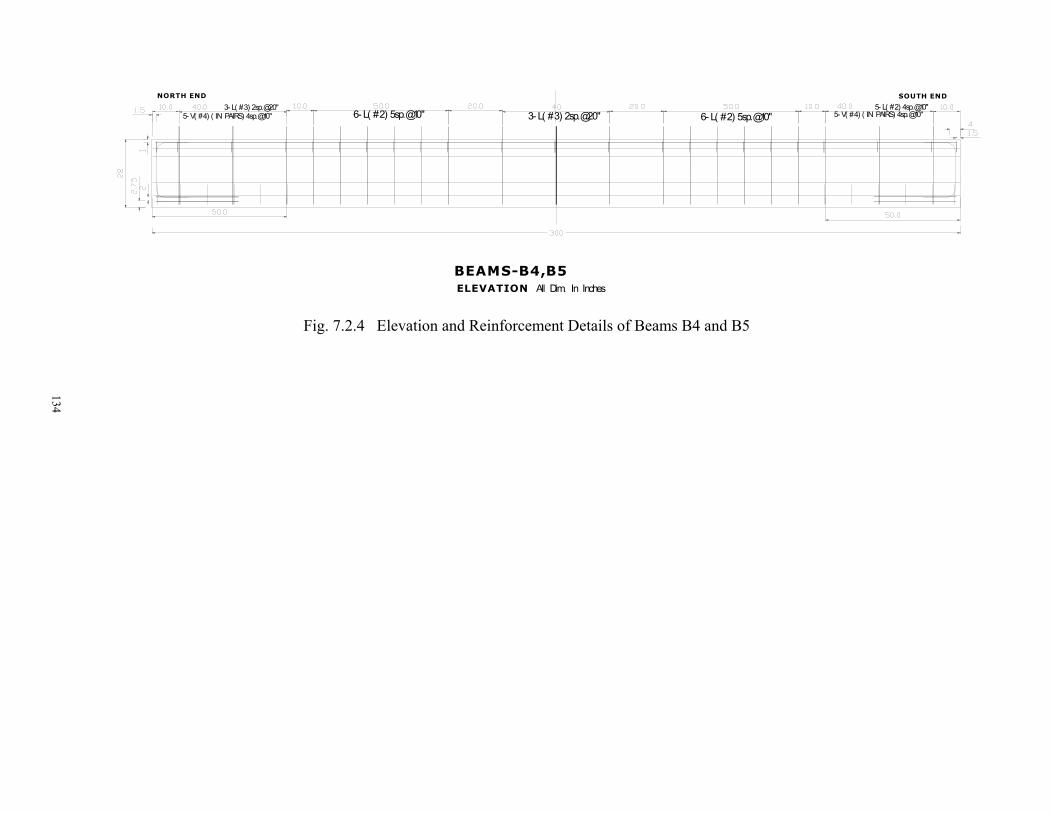
134

Fig. 7.2.4 Elevation and Reinforcement Details of Beams B4 and B5

NORTH END SOUTH END

3- L( #3) 2sp.@20" 6- L( #2) 5sp.@10"

BEAMS-B4,B5 ELEVATION All Dim. In Inches

6- L( #2) 5sp.@10" 5- L( #2) 4sp.@10"

5- V( #4) ( IN PAIRS) 4sp.@10" 5- V( #4) ( IN PAIRS) 4sp.@10" 3- L( #3) 2sp.@20"

134

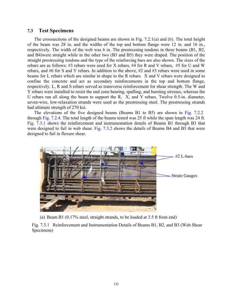
135

7.3 Test Specimens

The crosssections of the designed beams are shown in Fig. 7.2.1(a) and (b). The total height of the beam was 28 in. and the widths of the top and bottom flange were 12 in. and 16 in., respectively. The width of the web was 6 in. The prestressing tendons in three beams (B1, B2, and B4)were straight while in the other two (B3 and B5) they were draped. The position of the straight prestressing tendons and the type of the reinforcing bars are also shown. The sizes of the rebars are as follows: #3 rebars were used for X rebars, #4 for R and V rebars, #5 for U and W rebars, and #6 for S and Y rebars. In addition to the above, #2 and #3 rebars were used in some beams for L rebars which are similar in shape to the R rebars. X and V rebars were designed to confine the concrete and act as secondary reinforcements in the top and bottom flange, respectively. L, R and S rebars served as transverse reinforcement for shear strength. The W and Y rebars were installed to resist the end zone bearing, spalling, and bursting stresses, whereas the U rebars ran all along the beam to support the R, X, and Y rebars. Twelve 0.5-in. diameter, seven-wire, low-relaxation strands were used as the prestressing steel. The prestressing strands had ultimate strength of 270 ksi.

The elevations of the five designed beams (Beams B1 to B5) are shown in Fig. 7.2.2 through Fig. 7.2.4. The total length of the beams tested was 25 ft while the span length was 24 ft. Fig. 7.3.1 shows the reinforcement and instrumentation details of Beams B1 through B3 that were designed to fail in web shear. Fig. 7.3.2 shows the details of Beams B4 and B5 that were designed to fail in flexure shear.

(a) Beam B1 (0.17% steel, straight strands, to be loaded at 3.5 ft from end)

Fig. 7.3.1 Reinforcement and Instrumentation Details of Beams B1, B2, and B3 (Web Shear Specimens)

Strain Gauges

#2 L-bars

136

(b) Beam B2 (1% steel, straight strands, to be loaded at 3.5 ft from end)

(c) Beam B3 (1% steel, draped strands, to be loaded at 3.5 ft from end)

Fig. 7.3.1 Reinforcement and Instrumentation Details of Beams B1, B2, and B3 (Web Shear Specimens) (continued)

Strain Gauges

#4 R-bars

Strain Gauges

#4 R-bars

Draped Strands

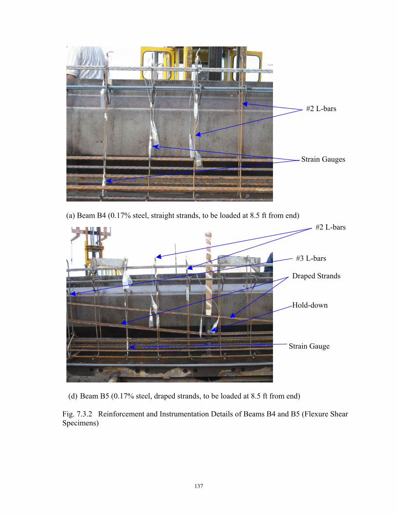
137

(a) Beam B4 (0.17% steel, straight strands, to be loaded at 8.5 ft from end)

(d) Beam B5 (0.17% steel, draped strands, to be loaded at 8.5 ft from end)

Fig. 7.3.2 Reinforcement and Instrumentation Details of Beams B4 and B5 (Flexure Shear Specimens)

Strain Gauges

#2 L-bars

Strain Gauge

#2 L-bars

Draped Strands

#3 L-bars

Hold-down

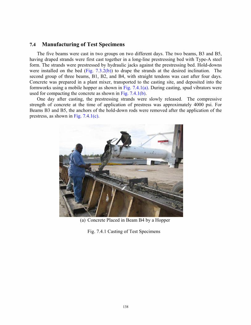
138

7.4 Manufacturing of Test Specimens

The five beams were cast in two groups on two different days. The two beams, B3 and B5, having draped strands were first cast together in a long-line prestressing bed with Type-A steel form. The strands were prestressed by hydraulic jacks against the prestressing bed. Hold-downs were installed on the bed (Fig. 7.3.2(b)) to drape the strands at the desired inclination. The second group of three beams, B1, B2, and B4, with straight tendons was cast after four days. Concrete was prepared in a plant mixer, transported to the casting site, and deposited into the formworks using a mobile hopper as shown in Fig. 7.4.1(a). During casting, spud vibrators were used for compacting the concrete as shown in Fig. 7.4.1(b).

One day after casting, the prestressing strands were slowly released. The compressive strength of concrete at the time of application of prestress was approximately 4000 psi. For Beams B3 and B5, the anchors of the hold-down rods were removed after the application of the prestress, as shown in Fig. 7.4.1(c).

(a) Concrete Placed in Beam B4 by a Hopper

Fig. 7.4.1 Casting of Test Specimens

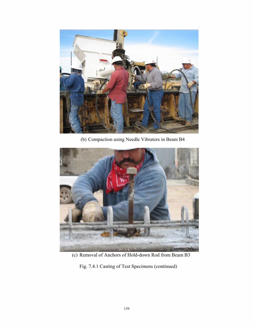
139

(b) Compaction using Needle Vibrators in Beam B4

(c) Removal of Anchors of Hold-down Rod from Beam B3

Fig. 7.4.1 Casting of Test Specimens (continued)

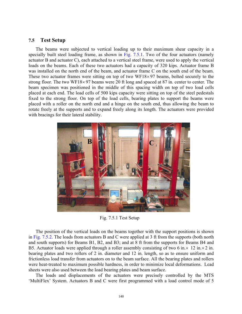
140

7.5 Test Setup

The beams were subjected to vertical loading up to their maximum shear capacity in a specially built steel loading frame, as shown in Fig. 7.5.1. Two of the four actuators (namely actuator B and actuator C), each attached to a vertical steel frame, were used to apply the vertical loads on the beams. Each of these two actuators had a capacity of 320 kips. Actuator frame B was installed on the north end of the beam, and actuator frame C on the south end of the beam. These two actuator frames were sitting on top of two WF18×97 beams, bolted securely to the strong floor. The two WF18×97 beams were 20 ft long and spaced at 87 in. center to center. The beam specimen was positioned in the middle of this spacing width on top of two load cells placed at each end. The load cells of 500 kips capacity were sitting on top of the steel pedestals fixed to the strong floor. On top of the load cells, bearing plates to support the beams were placed with a roller on the north end and a hinge on the south end, thus allowing the beam to rotate freely at the supports and to expand freely along its length. The actuators were provided with bracings for their lateral stability.

Fig. 7.5.1 Test Setup

The position of the vertical loads on the beams together with the support positions is shown in Fig. 7.5.2. The loads from actuators B and C were applied at 3 ft from the supports (both north and south supports) for Beams B1, B2, and B3; and at 8 ft from the supports for Beams B4 and B5. Actuator loads were applied through a roller assembly consisting of two 6 in.× 12 in.×2 in. bearing plates and two rollers of 2 in. diameter and 12 in. length, so as to ensure uniform and frictionless load transfer from actuators on to the beam surface. All the bearing plates and rollers were heat-treated to maximum possible hardness, in order to minimize local deformations. Lead sheets were also used between the load bearing plates and beam surface.

The loads and displacements of the actuators were precisely controlled by the MTS ‘MultiFlex’ System. Actuators B and C were first programmed with a load control mode of 5

B C

141

kips/min. When the slope of the load-displacement curve started decreasing, the control mode was switched to a displacement control of 0.2 in./hour. This step continued until shear failure occurred at either end of the beam. This displacement control feature was essential in capturing the ductility/brittleness behavior of the beam failing in shear.

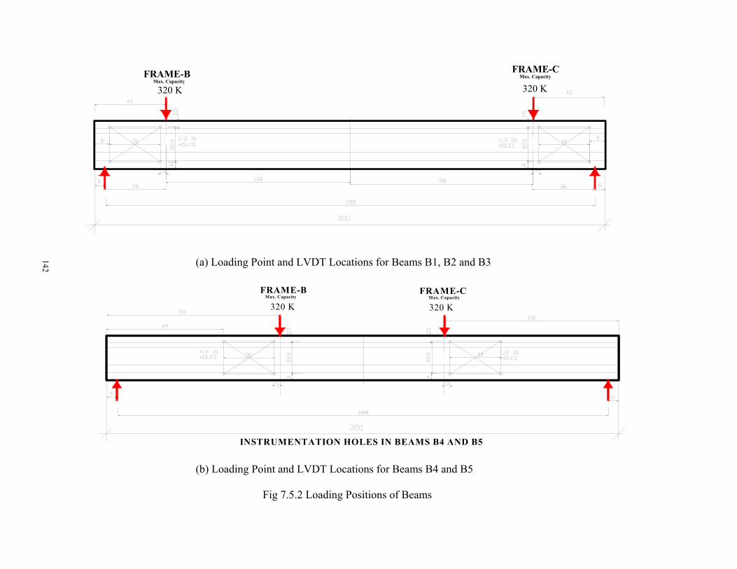
142

(a) Loading Point and LVDT Locations for Beams B1, B2 and B3

(b) Loading Point and LVDT Locations for Beams B4 and B5

Fig 7.5.2 Loading Positions of Beams

320 KMax. Capacity

Max. Capacity

320 K

FRAME-CFRAME-B

INSTRUMENTATION HOLES IN BEAMS B4 AND B5

320 K 320 K

FRAME-CFRAME-BMax. Capacity Max. Capacity

142

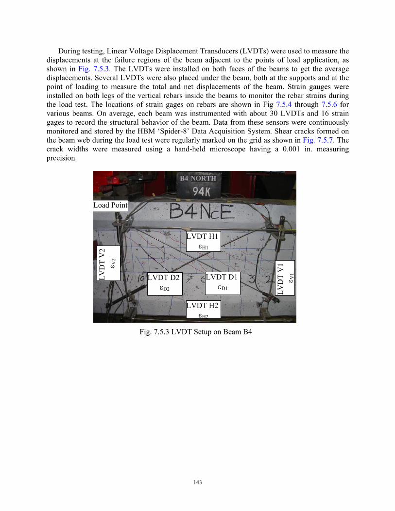
143

During testing, Linear Voltage Displacement Transducers (LVDTs) were used to measure the displacements at the failure regions of the beam adjacent to the points of load application, as shown in Fig. 7.5.3. The LVDTs were installed on both faces of the beams to get the average displacements. Several LVDTs were also placed under the beam, both at the supports and at the point of loading to measure the total and net displacements of the beam. Strain gauges were installed on both legs of the vertical rebars inside the beams to monitor the rebar strains during the load test. The locations of strain gages on rebars are shown in Fig 7.5.4 through 7.5.6 for various beams. On average, each beam was instrumented with about 30 LVDTs and 16 strain gages to record the structural behavior of the beam. Data from these sensors were continuously monitored and stored by the HBM ‘Spider-8’ Data Acquisition System. Shear cracks formed on the beam web during the load test were regularly marked on the grid as shown in Fig. 7.5.7. The crack widths were measured using a hand-held microscope having a 0.001 in. measuring precision.

Fig. 7.5.3 LVDT Setup on Beam B4

LVDT H2εH2

LVD

T V

1 ε V

1 LVD

T V

2 ε V

2

LVDT H1εH1

Load Point

LVDT D1εD1

LVDT D2εD2

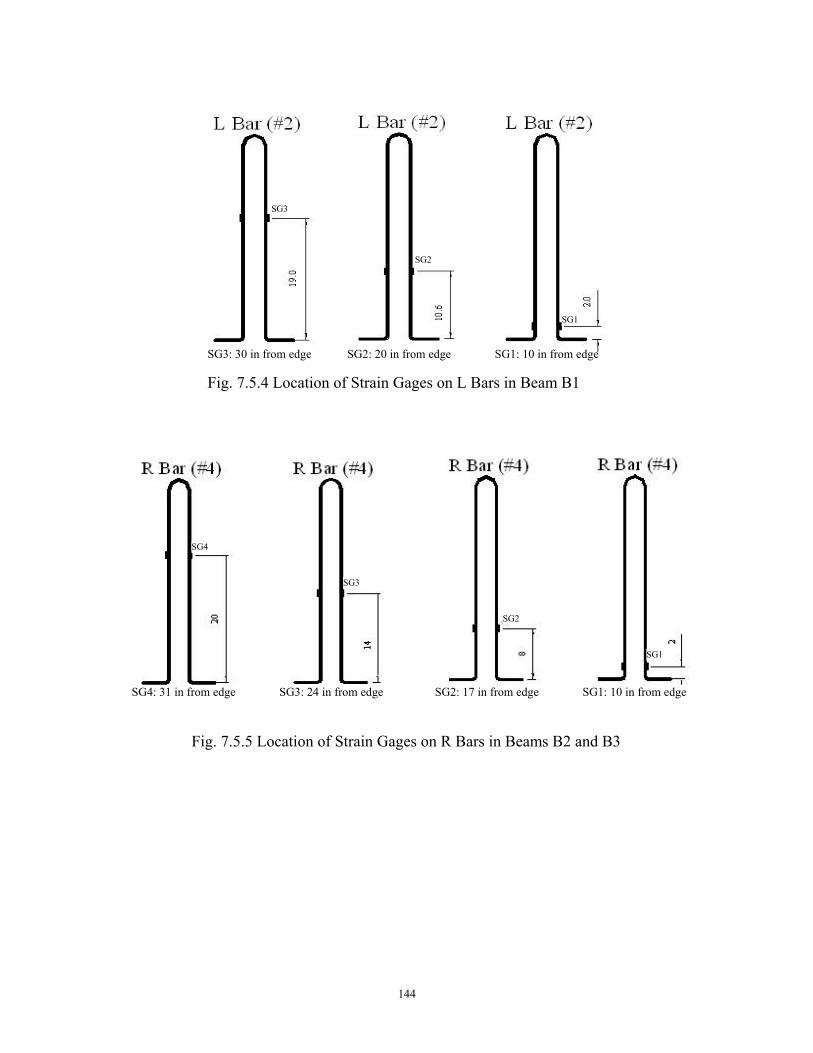
144

Fig. 7.5.4 Location of Strain Gages on L Bars in Beam B1

Fig. 7.5.5 Location of Strain Gages on R Bars in Beams B2 and B3

SG1: 10 in from edge SG2: 20 in from edgeSG3: 30 in from edge

SG1: 10 in from edgeSG2: 17 in from edgeSG3: 24 in from edgeSG4: 31 in from edge

SG1

SG2

SG3

SG1

SG2

SG3

SG4

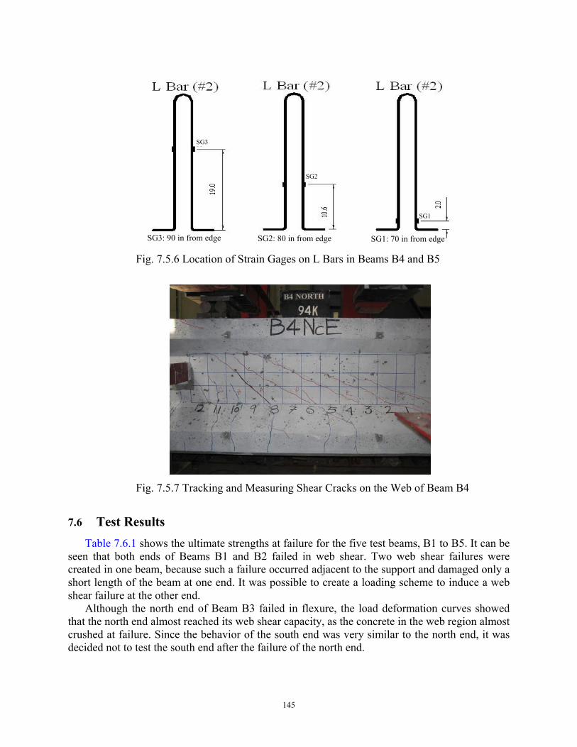
145

Fig. 7.5.6 Location of Strain Gages on L Bars in Beams B4 and B5

Fig. 7.5.7 Tracking and Measuring Shear Cracks on the Web of Beam B4

7.6 Test Results

Table 7.6.1 shows the ultimate strengths at failure for the five test beams, B1 to B5. It can be seen that both ends of Beams B1 and B2 failed in web shear. Two web shear failures were created in one beam, because such a failure occurred adjacent to the support and damaged only a short length of the beam at one end. It was possible to create a loading scheme to induce a web shear failure at the other end.

Although the north end of Beam B3 failed in flexure, the load deformation curves showed that the north end almost reached its web shear capacity, as the concrete in the web region almost crushed at failure. Since the behavior of the south end was very similar to the north end, it was decided not to test the south end after the failure of the north end.

SG1: 70 in from edge SG2: 80 in from edgeSG3: 90 in from edge

SG1

SG2

SG3

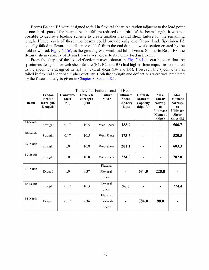
146

Beams B4 and B5 were designed to fail in flexural shear in a region adjacent to the load point at one-third span of the beams. As the failure reduced one-third of the beam length, it was not possible to devise a loading scheme to create another flexural shear failure for the remaining length. Hence, each of these two beams could provide only one failure load. Specimen B5 actually failed in flexure at a distance of 11 ft from the end due to a weak section created by the hold-down rod, Fig. 7.4.1(c), as the grouting was weak and full of voids. Similar to Beam B3, the flexural shear capacity of Beam B5 was very close to its failure load in flexure.

From the shape of the load-deflection curves, shown in Fig. 7.6.1. it can be seen that the specimens designed for web shear failure (B1, B2, and B3) had higher shear capacities compared to the specimens designed to fail in flexural shear (B4 and B5). However, the specimens that failed in flexural shear had higher ductility. Both the strength and deflections were well predicted by the flexural analysis given in Chapter 8, Section 8.1.

Table 7.6.1 Failure Loads of Beams

Beam

Tendon Profile

(Straight/ Draped)

Transverse Steel (%)

Concrete Strength

(ksi)

Failure Mode

Ultimate Shear

Capacity (kips)

Ultimate Moment Capacity (kips-ft.)

Max. Shear

corresp. to

Ultimate Moment

(kips)

Max. Moment corresp.

to Ultimate

Shear (kips-ft.)

B1-North

Straight 0.17 10.5 Web-Shear 188.9 - - 566.7

B1-South


B2-North


B2-South


B3-North

Draped 1.0 9.37

Flexure/

Flexural-

Shear

- 684.0 228.0 -

B4-South

Straight 0.17 10.3

Flexural-

Shear 96.8 - - 774.4

B5-North

Draped 0.17 9.36

Flexure/

Flexural-

Shear

- 784.0 98.0 -

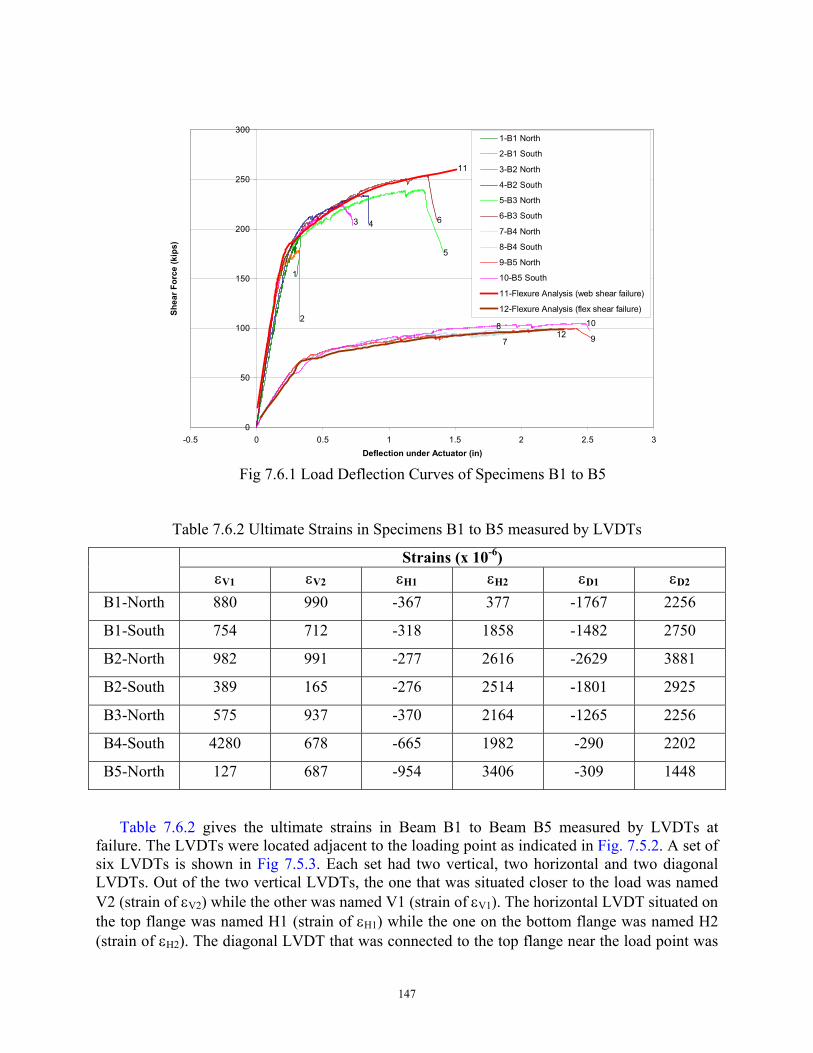
147

Fig 7.6.1 Load Deflection Curves of Specimens B1 to B5

Table 7.6.2 Ultimate Strains in Specimens B1 to B5 measured by LVDTs

Strains (x 10-6) εV1 εV2 εH1 εH2 εD1 εD2

B1-North 880 990 -367 377 -1767 2256

B1-South 754 712 -318 1858 -1482 2750

B2-North 982 991 -277 2616 -2629 3881

B2-South 389 165 -276 2514 -1801 2925

B3-North 575 937 -370 2164 -1265 2256

B4-South 4280 678 -665 1982 -290 2202

B5-North 127 687 -954 3406 -309 1448

Table 7.6.2 gives the ultimate strains in Beam B1 to Beam B5 measured by LVDTs at failure. The LVDTs were located adjacent to the loading point as indicated in Fig. 7.5.2. A set of six LVDTs is shown in Fig 7.5.3. Each set had two vertical, two horizontal and two diagonal LVDTs. Out of the two vertical LVDTs, the one that was situated closer to the load was named V2 (strain of εV2) while the other was named V1 (strain of εV1). The horizontal LVDT situated on the top flange was named H1 (strain of εH1) while the one on the bottom flange was named H2 (strain of εH2). The diagonal LVDT that was connected to the top flange near the load point was

1

2

3 4

5

6

7

89

10

11

12

0

50

100

150

200

250

300

-0.5 0 0.5 1 1.5 2 2.5 3Deflection under Actuator (in)

Shea

r For

ce (k

ips)

1-B1 North

2-B1 South

3-B2 North

4-B2 South

5-B3 North

6-B3 South

7-B4 North

8-B4 South

9-B5 North

10-B5 South

11-Flexure Analysis (web shear failure)

12-Flexure Analysis (flex shear failure)

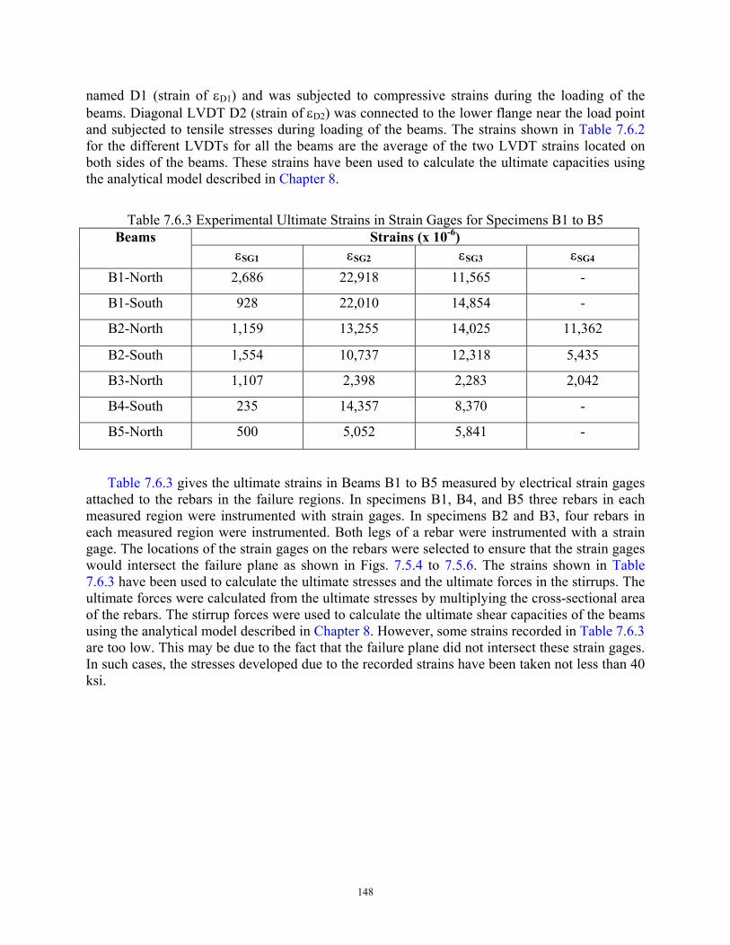
148

named D1 (strain of εD1) and was subjected to compressive strains during the loading of the beams. Diagonal LVDT D2 (strain of εD2) was connected to the lower flange near the load point and subjected to tensile stresses during loading of the beams. The strains shown in Table 7.6.2 for the different LVDTs for all the beams are the average of the two LVDT strains located on both sides of the beams. These strains have been used to calculate the ultimate capacities using the analytical model described in Chapter 8.

Table 7.6.3 Experimental Ultimate Strains in Strain Gages for Specimens B1 to B5 Strains (x 10-6) Beams

εSG1 εSG2 εSG3 εSG4 B1-North 2,686 22,918 11,565 -

B1-South 928 22,010 14,854 -

B2-North 1,159 13,255 14,025 11,362

B2-South 1,554 10,737 12,318 5,435

B3-North 1,107 2,398 2,283 2,042

B4-South 235 14,357 8,370 -

B5-North 500 5,052 5,841 -

Table 7.6.3 gives the ultimate strains in Beams B1 to B5 measured by electrical strain gages attached to the rebars in the failure regions. In specimens B1, B4, and B5 three rebars in each measured region were instrumented with strain gages. In specimens B2 and B3, four rebars in each measured region were instrumented. Both legs of a rebar were instrumented with a strain gage. The locations of the strain gages on the rebars were selected to ensure that the strain gages would intersect the failure plane as shown in Figs. 7.5.4 to 7.5.6. The strains shown in Table 7.6.3 have been used to calculate the ultimate stresses and the ultimate forces in the stirrups. The ultimate forces were calculated from the ultimate stresses by multiplying the cross-sectional area of the rebars. The stirrup forces were used to calculate the ultimate shear capacities of the beams using the analytical model described in Chapter 8. However, some strains recorded in Table 7.6.3 are too low. This may be due to the fact that the failure plane did not intersect these strain gages. In such cases, the stresses developed due to the recorded strains have been taken not less than 40 ksi.

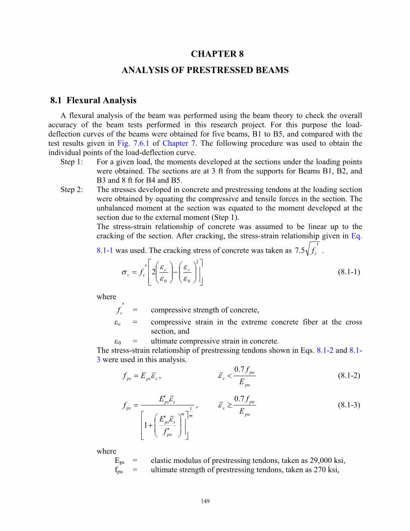
149

CHAPTER 8

ANALYSIS OF PRESTRESSED BEAMS

8.1 Flexural Analysis A flexural analysis of the beam was performed using the beam theory to check the overall

accuracy of the beam tests performed in this research project. For this purpose the load-deflection curves of the beams were obtained for five beams, B1 to B5, and compared with the test results given in Fig. 7.6.1 of Chapter 7. The following procedure was used to obtain the individual points of the load-deflection curve.

Step 1: For a given load, the moments developed at the sections under the loading points were obtained. The sections are at 3 ft from the supports for Beams B1, B2, and B3 and 8 ft for B4 and B5.

Step 2: The stresses developed in concrete and prestressing tendons at the loading section were obtained by equating the compressive and tensile forces in the section. The unbalanced moment at the section was equated to the moment developed at the section due to the external moment (Step 1). The stress-strain relationship of concrete was assumed to be linear up to the cracking of the section. After cracking, the stress-strain relationship given in Eq.

8.1-1 was used. The cracking stress of concrete was taken as ′cf5.7 .

−

′=2

00

2εε

εε

σ cccc f (8.1-1)

where ′

cf = compressive strength of concrete, εc = compressive strain in the extreme concrete fiber at the cross

section, and ε0 = ultimate compressive strain in concrete.

The stress-strain relationship of prestressing tendons shown in Eqs. 8.1-2 and 8.1-3 were used in this analysis.

spsps Ef ε= , pu

pus E

f7.0<ε (8.1-2)

mm

pu

sps

spsps

fE

Ef 1

1

′

′+

′=

ε

ε,

pu

pus E

f7.0≥ε (8.1-3)

where Eps = elastic modulus of prestressing tendons, taken as 29,000 ksi,

fpu = ultimate strength of prestressing tendons, taken as 270 ksi,

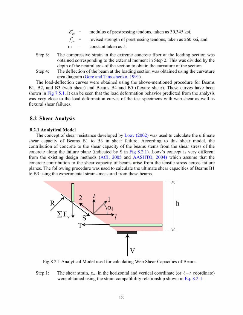
150

psE′ = modulus of prestressing tendons, taken as 30,345 ksi, puf ′ = revised strength of prestressing tendons, taken as 260 ksi, and m = constant taken as 5.

Step 3: The compressive strain in the extreme concrete fiber at the loading section was obtained corresponding to the external moment in Step 2. This was divided by the depth of the neutral axis of the section to obtain the curvature of the section.

Step 4: The deflection of the beam at the loading section was obtained using the curvature area diagram (Gere and Timoshenko, 1991).

The load-deflection curves were obtained using the above-mentioned procedure for Beams B1, B2, and B3 (web shear) and Beams B4 and B5 (flexure shear). These curves have been shown in Fig 7.5.1. It can be seen that the load deformation behavior predicted from the analysis was very close to the load deformation curves of the test specimens with web shear as well as flexural shear failures.

8.2 Shear Analysis 8.2.1 Analytical Model

The concept of shear resistance developed by Loov (2002) was used to calculate the ultimate shear capacity of Beams B1 to B3 in shear failure. According to this shear model, the contribution of concrete to the shear capacity of the beams stems from the shear stress of the concrete along the failure plane (indicated by S in Fig 8.2.1). Loov’s concept is very different from the existing design methods (ACI, 2005 and AASHTO, 2004) which assume that the concrete contribution to the shear capacity of beams arise from the tensile stress across failure planes. The following procedure was used to calculate the ultimate shear capacities of Beams B1 to B3 using the experimental strains measured from these beams.

Fig 8.2.1 Analytical Model used for calculating Web Shear Capacities of Beams

Step 1: The shear strain, γhv, in the horizontal and vertical coordinate (or t−l coordinate) were obtained using the strain compatibility relationship shown in Eq. 8.2-1:

h

V

R α1

ST

∑ vF l

t 12

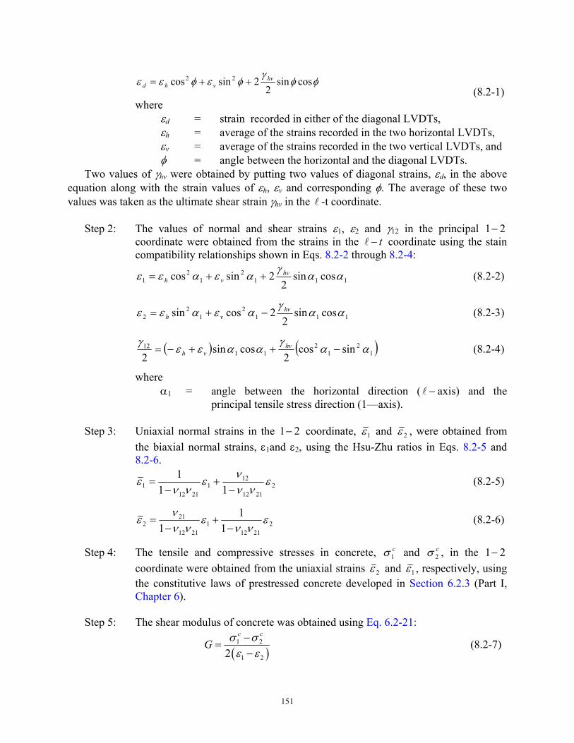
151

φφγ

φεφεε cossin2

2sincos 22 hvvhd ++=

(8.2-1) where

εd = strain recorded in either of the diagonal LVDTs, εh = average of the strains recorded in the two horizontal LVDTs, εv = average of the strains recorded in the two vertical LVDTs, and φ = angle between the horizontal and the diagonal LVDTs.

Two values of γhv were obtained by putting two values of diagonal strains, εd, in the above equation along with the strain values of εh, εv and corresponding φ. The average of these two values was taken as the ultimate shear strain γhv in the l -t coordinate.

Step 2: The values of normal and shear strains ε1, ε2 and γ12 in the principal 21− coordinate were obtained from the strains in the t−l coordinate using the stain compatibility relationships shown in Eqs. 8.2-2 through 8.2-4:

1112

12

1 cossin2

2sincos ααγ

αεαεε hvvh ++= (8.2-2)

1112

12

2 cossin2

2cossin ααγ

αεαεε hvvh −+= (8.2-3)

( ) ( )12

12

1112 sincos

2cossin

2αα

γααεε

γ−++−= hv

vh (8.2-4)

where α1 = angle between the horizontal direction ( −l axis) and the

principal tensile stress direction (1—axis). Step 3: Uniaxial normal strains in the 21− coordinate, 1ε and 2ε , were obtained from

the biaxial normal strains, ε1and ε2, using the Hsu-Zhu ratios in Eqs. 8.2-5 and 8.2-6.

22112

121

21121 11

1 ενν

νε

ννε

−+

−= (8.2-5)

22112

12112

212 1

11

ενν

ενν

νε−

+−

= (8.2-6)

Step 4: The tensile and compressive stresses in concrete, c1σ and c

2σ , in the 21− coordinate were obtained from the uniaxial strains 2ε and 1ε , respectively, using the constitutive laws of prestressed concrete developed in Section 6.2.3 (Part I, Chapter 6).

Step 5: The shear modulus of concrete was obtained using Eq. 6.2-21:

( )1 2

1 22

c c

G σ σε ε

−=

− (8.2-7)

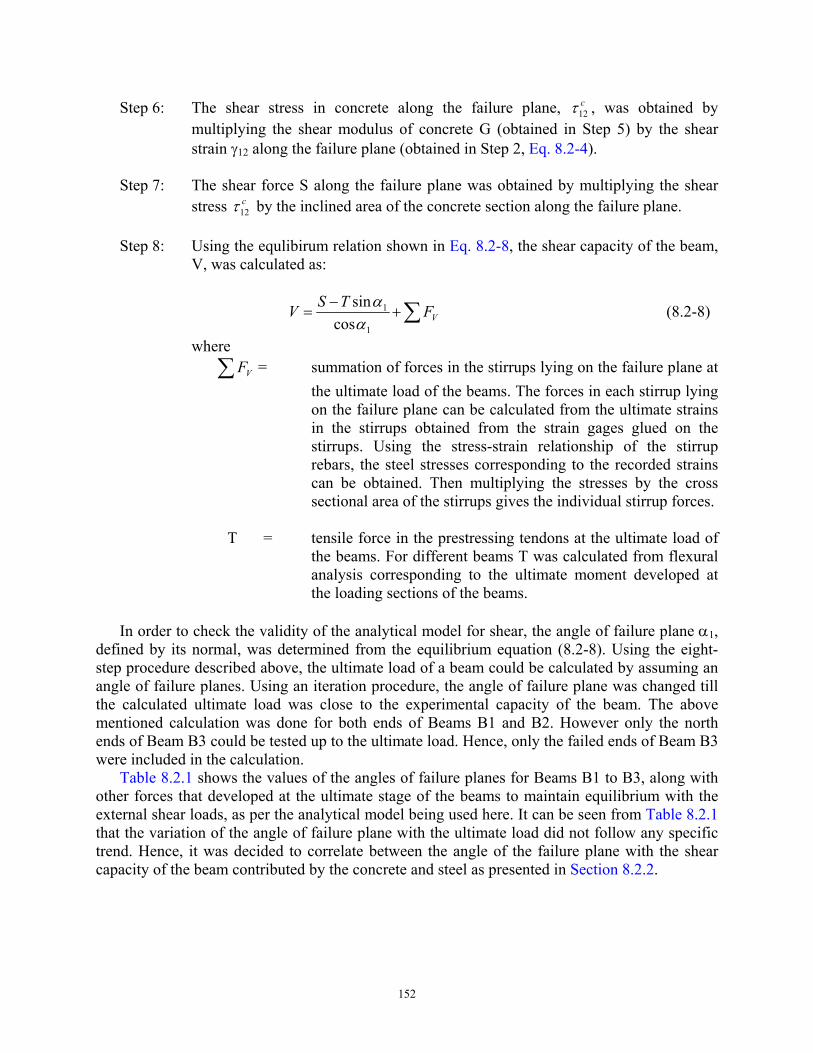
152

Step 6: The shear stress in concrete along the failure plane, c12τ , was obtained by

multiplying the shear modulus of concrete G (obtained in Step 5) by the shear strain γ12 along the failure plane (obtained in Step 2, Eq. 8.2-4).

Step 7: The shear force S along the failure plane was obtained by multiplying the shear

stress c12τ by the inclined area of the concrete section along the failure plane.

Step 8: Using the equlibirum relation shown in Eq. 8.2-8, the shear capacity of the beam,

V, was calculated as:

∑+−

= VFTSV1

1

cossinα

α (8.2-8)

where ∑ VF = summation of forces in the stirrups lying on the failure plane at

the ultimate load of the beams. The forces in each stirrup lying on the failure plane can be calculated from the ultimate strains in the stirrups obtained from the strain gages glued on the stirrups. Using the stress-strain relationship of the stirrup rebars, the steel stresses corresponding to the recorded strains can be obtained. Then multiplying the stresses by the cross sectional area of the stirrups gives the individual stirrup forces.

T = tensile force in the prestressing tendons at the ultimate load of

the beams. For different beams T was calculated from flexural analysis corresponding to the ultimate moment developed at the loading sections of the beams.

In order to check the validity of the analytical model for shear, the angle of failure plane α1,

defined by its normal, was determined from the equilibrium equation (8.2-8). Using the eight-step procedure described above, the ultimate load of a beam could be calculated by assuming an angle of failure planes. Using an iteration procedure, the angle of failure plane was changed till the calculated ultimate load was close to the experimental capacity of the beam. The above mentioned calculation was done for both ends of Beams B1 and B2. However only the north ends of Beam B3 could be tested up to the ultimate load. Hence, only the failed ends of Beam B3 were included in the calculation.

Table 8.2.1 shows the values of the angles of failure planes for Beams B1 to B3, along with other forces that developed at the ultimate stage of the beams to maintain equilibrium with the external shear loads, as per the analytical model being used here. It can be seen from Table 8.2.1 that the variation of the angle of failure plane with the ultimate load did not follow any specific trend. Hence, it was decided to correlate between the angle of the failure plane with the shear capacity of the beam contributed by the concrete and steel as presented in Section 8.2.2.

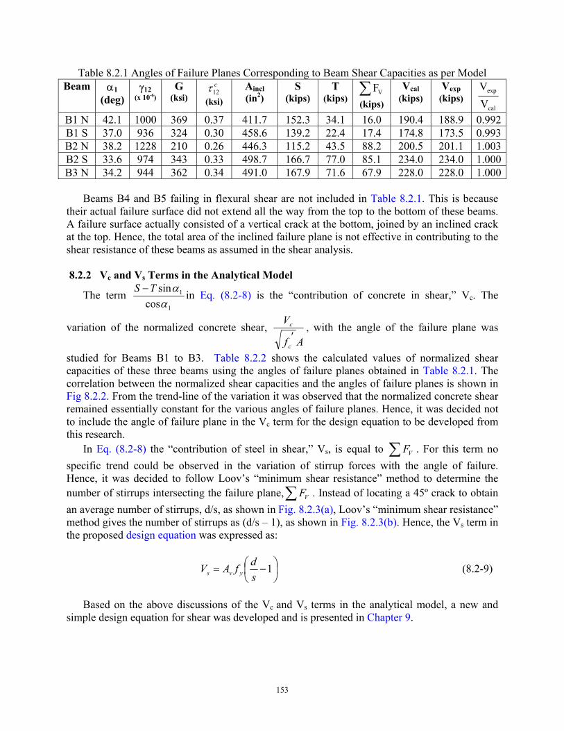
153

Table 8.2.1 Angles of Failure Planes Corresponding to Beam Shear Capacities as per Model Beam α1

(deg) γ12

(x 10-6) G

(ksi) c12τ

(ksi) Aincl (in2)

S (kips)

T (kips)

∑ VF(kips)

Vcal (kips)

Vexp (kips)

cal

exp

VV

B1 N 42.1 1000 369 0.37 411.7 152.3 34.1 16.0 190.4 188.9 0.992B1 S 37.0 936 324 0.30 458.6 139.2 22.4 17.4 174.8 173.5 0.993B2 N 38.2 1228 210 0.26 446.3 115.2 43.5 88.2 200.5 201.1 1.003B2 S 33.6 974 343 0.33 498.7 166.7 77.0 85.1 234.0 234.0 1.000B3 N 34.2 944 362 0.34 491.0 167.9 71.6 67.9 228.0 228.0 1.000

Beams B4 and B5 failing in flexural shear are not included in Table 8.2.1. This is because

their actual failure surface did not extend all the way from the top to the bottom of these beams. A failure surface actually consisted of a vertical crack at the bottom, joined by an inclined crack at the top. Hence, the total area of the inclined failure plane is not effective in contributing to the shear resistance of these beams as assumed in the shear analysis.

8.2.2 Vc and Vs Terms in the Analytical Model

The term 1

1

cossinα

αTS − in Eq. (8.2-8) is the “contribution of concrete in shear,” Vc. The

variation of the normalized concrete shear, Af

V

c

c

′, with the angle of the failure plane was

studied for Beams B1 to B3. Table 8.2.2 shows the calculated values of normalized shear capacities of these three beams using the angles of failure planes obtained in Table 8.2.1. The correlation between the normalized shear capacities and the angles of failure planes is shown in Fig 8.2.2. From the trend-line of the variation it was observed that the normalized concrete shear remained essentially constant for the various angles of failure planes. Hence, it was decided not to include the angle of failure plane in the Vc term for the design equation to be developed from this research.

In Eq. (8.2-8) the “contribution of steel in shear,” Vs, is equal to VF∑ . For this term no specific trend could be observed in the variation of stirrup forces with the angle of failure. Hence, it was decided to follow Loov’s “minimum shear resistance” method to determine the number of stirrups intersecting the failure plane, VF∑ . Instead of locating a 45º crack to obtain an average number of stirrups, d/s, as shown in Fig. 8.2.3(a), Loov’s “minimum shear resistance” method gives the number of stirrups as (d/s – 1), as shown in Fig. 8.2.3(b). Hence, the Vs term in the proposed design equation was expressed as:

−= 1

sdfAV yvs (8.2-9)

Based on the above discussions of the Vc and Vs terms in the analytical model, a new and simple design equation for shear was developed and is presented in Chapter 9.

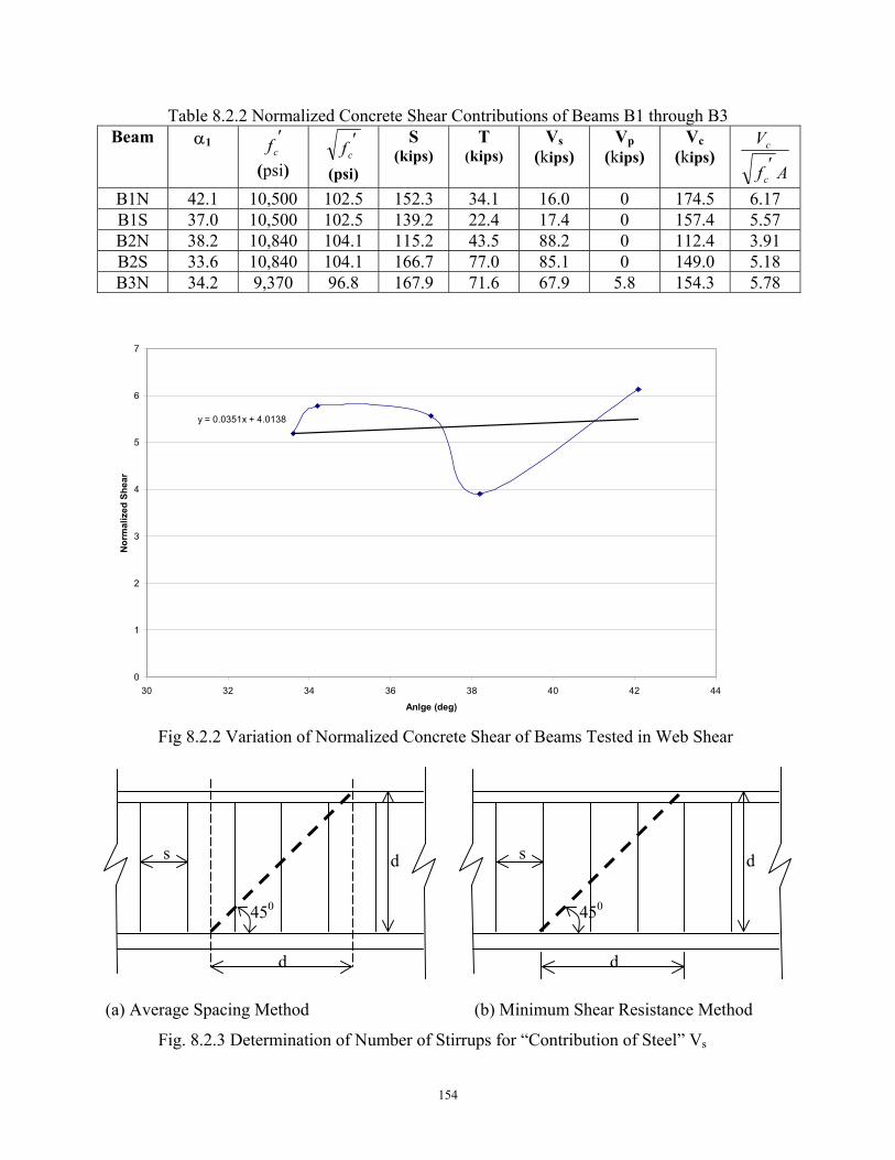
154

Table 8.2.2 Normalized Concrete Shear Contributions of Beams B1 through B3 Beam α1 ′

cf (psi)

′cf

(psi)

S (kips)

T (kips)

Vs (kips)

Vp (kips)

Vc (kips)

Af

V

c

c

′

B1N 42.1 10,500 102.5 152.3 34.1 16.0 0 174.5 6.17 B1S 37.0 10,500 102.5 139.2 22.4 17.4 0 157.4 5.57 B2N 38.2 10,840 104.1 115.2 43.5 88.2 0 112.4 3.91 B2S 33.6 10,840 104.1 166.7 77.0 85.1 0 149.0 5.18 B3N 34.2 9,370 96.8 167.9 71.6 67.9 5.8 154.3 5.78

Fig 8.2.2 Variation of Normalized Concrete Shear of Beams Tested in Web Shear

(a) Average Spacing Method (b) Minimum Shear Resistance Method

Fig. 8.2.3 Determination of Number of Stirrups for “Contribution of Steel” Vs

y = 0.0351x + 4.0138

0

1

2

3

4

5

6

7

30 32 34 36 38 40 42 44

Anlge (deg)

Nor

mal

ized

She

ar

d

d s

450

d

d s

450

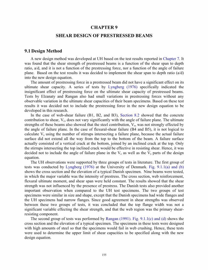
155

CHAPTER 9

SHEAR DESIGN OF PRESTRESSED BEAMS

9.1 Design Method

A new design method was developed at UH based on the test results reported in Chapter 7. It was found that the shear strength of prestressed beams is a function of the shear span to depth ratio, a/d, and it is not a function of the prestressing force, nor a function of the angle of failure plane. Based on the test results it was decided to implement the shear span to depth ratio (a/d) into the new design equation.

The amount of prestressing force in a prestressed beam did not have a significant effect on its ultimate shear capacity. A series of tests by Lyngberg (1976) specifically indicated the insignificant effect of prestressing force on the ultimate shear capacity of prestressed beams. Tests by Elzanaty and Rangan also had small variations in prestressing forces without any observable variation in the ultimate shear capacities of their beam specimens. Based on these test results it was decided not to include the prestressing force in the new design equation to be developed in this research.

In the case of web-shear failure (B1, B2, and B3), Section 8.2 showed that the concrete contribution to shear, Vc, does not vary significantly with the angle of failure plane. The ultimate strengths of these beams also showed that the steel contribution, Vs, was not strongly effected by the angle of failure plane. In the case of flexural-shear failure (B4 and B5), it is not logical to calculate Vs using the number of stirrups intersecting a failure plane, because the actual failure surface did not extend all the way from the top to the bottom of the beam. A failure surface actually consisted of a vertical crack at the bottom, joined by an inclined crack at the top. Only the stirrups intersecting the top inclined crack would be effective in resisting shear. Hence, it was decided not to include the angle of failure plane in the Vc as well as the Vs parts of the design equation.

The UH observations were supported by three groups of tests in literature. The first group of tests was conducted by Lyngberg (1976) at the University of Denmark. Fig. 9.1.1(a) and (b) shows the cross section and the elevation of a typical Danish specimen. Nine beams were tested, in which the major variable was the intensity of prestress. The cross section, web reinforcement, flexural ultimate moment, and shear span were held constant. The results showed that the shear strength was not influenced by the presence of prestress. The Danish tests also provided another important observation when compared to the UH test specimens. The two groups of test specimens were similar in size and shape, except that the Danish specimens had wide flanges and the UH specimens had narrow flanges. Since good agreement in shear strengths was observed between these two groups of tests, it was concluded that the top flange width was not a significant variable effecting the shear strength, and that the web region was the primary shear-resisting component.

The second group of tests was performed by Rangan (1991). Fig. 9.1.1(c) and (d) shows the cross section and the elevation of a typical specimen. The specimens in these tests were designed with high amounts of steel so that the specimens would fail in web crushing. Hence, these tests were used to determine the upper limit of shear capacities to be specified along with the new design equation.

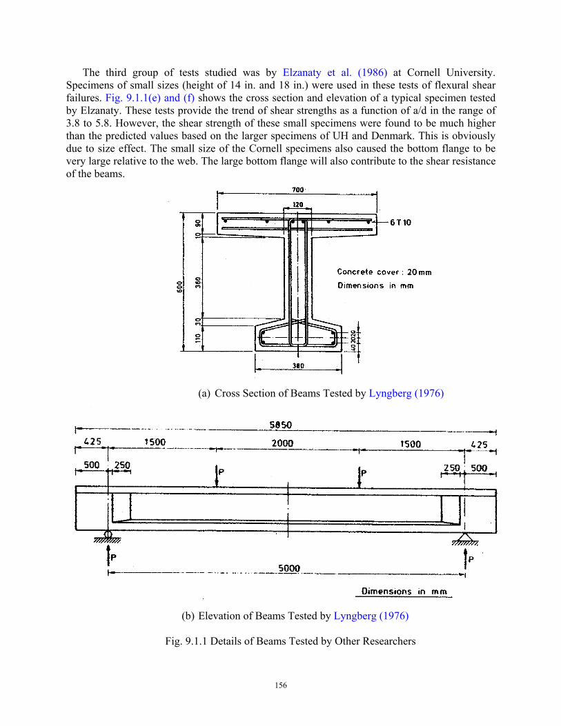
156

The third group of tests studied was by Elzanaty et al. (1986) at Cornell University. Specimens of small sizes (height of 14 in. and 18 in.) were used in these tests of flexural shear failures. Fig. 9.1.1(e) and (f) shows the cross section and elevation of a typical specimen tested by Elzanaty. These tests provide the trend of shear strengths as a function of a/d in the range of 3.8 to 5.8. However, the shear strength of these small specimens were found to be much higher than the predicted values based on the larger specimens of UH and Denmark. This is obviously due to size effect. The small size of the Cornell specimens also caused the bottom flange to be very large relative to the web. The large bottom flange will also contribute to the shear resistance of the beams.

(a) Cross Section of Beams Tested by Lyngberg (1976)

(b) Elevation of Beams Tested by Lyngberg (1976)

Fig. 9.1.1 Details of Beams Tested by Other Researchers

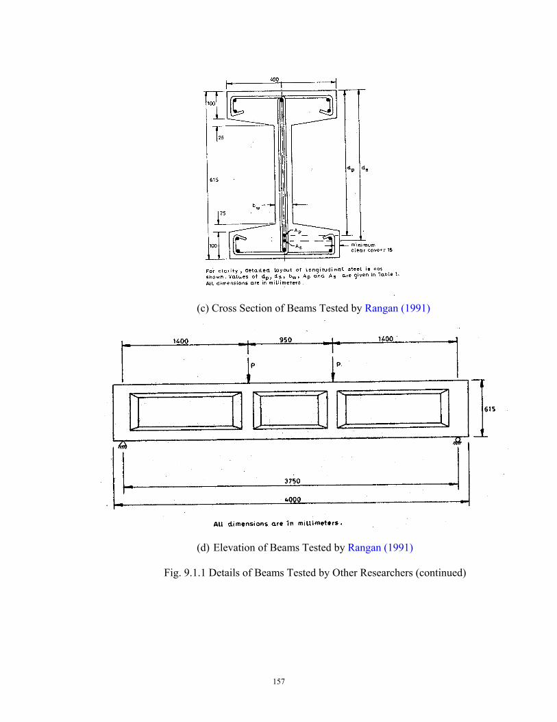
157

(c) Cross Section of Beams Tested by Rangan (1991)

(d) Elevation of Beams Tested by Rangan (1991)

Fig. 9.1.1 Details of Beams Tested by Other Researchers (continued)

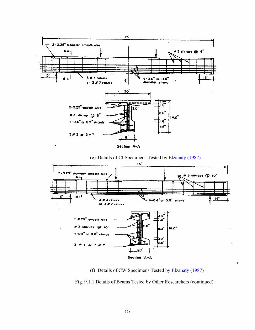
158

(e) Details of CI Specimens Tested by Elzanaty (1987)

(f) Details of CW Specimens Tested by Elzanaty (1987)

Fig. 9.1.1 Details of Beams Tested by Other Researchers (continued)

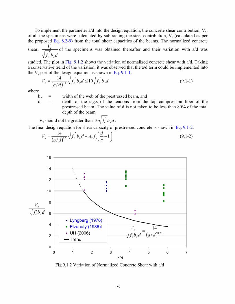
159

To implement the parameter a/d into the design equation, the concrete shear contribution, Vc, of all the specimens were calculated by subtracting the steel contribution, Vs (calculated as per the proposed Eq. 8.2-9) from the total shear capacities of the beams. The normalized concrete

shear, dbf

V

wc

c

′of the specimens was obtained thereafter and their variation with a/d was

studied. The plot in Fig. 9.1.2 shows the variation of normalized concrete shear with a/d. Taking a conservative trend of the variation, it was observed that the a/d term could be implemented into the Vc part of the design equation as shown in Eq. 9.1-1.

( )dbf

daV wcc

′= 7.0/14 dbf wc

′≤10 (9.1-1)

where bw = width of the web of the prestressed beam, and d = depth of the c.g.s of the tendons from the top compression fiber of the

prestressed beam. The value of d is not taken to be less than 80% of the total depth of the beam.

Vc should not be greater than dbf wc′10 .

The final design equation for shear capacity of prestressed concrete is shown in Eq. 9.1-2.

( )

−+′= 1

/14

7.0 sdfAdbf

daV yvwcu (9.1-2)

Fig 9.1.2 Variation of Normalized Concrete Shear with a/d

0

2

4

6

8

10

12

14

16

0 1 2 3 4 5 6 7a/d

Lyngberg (1976)Elzanaty (1986)lUH (2006)Trend

( ) 70.0/14dadbf

V

wc

c =′

dbfV

wc

c

′

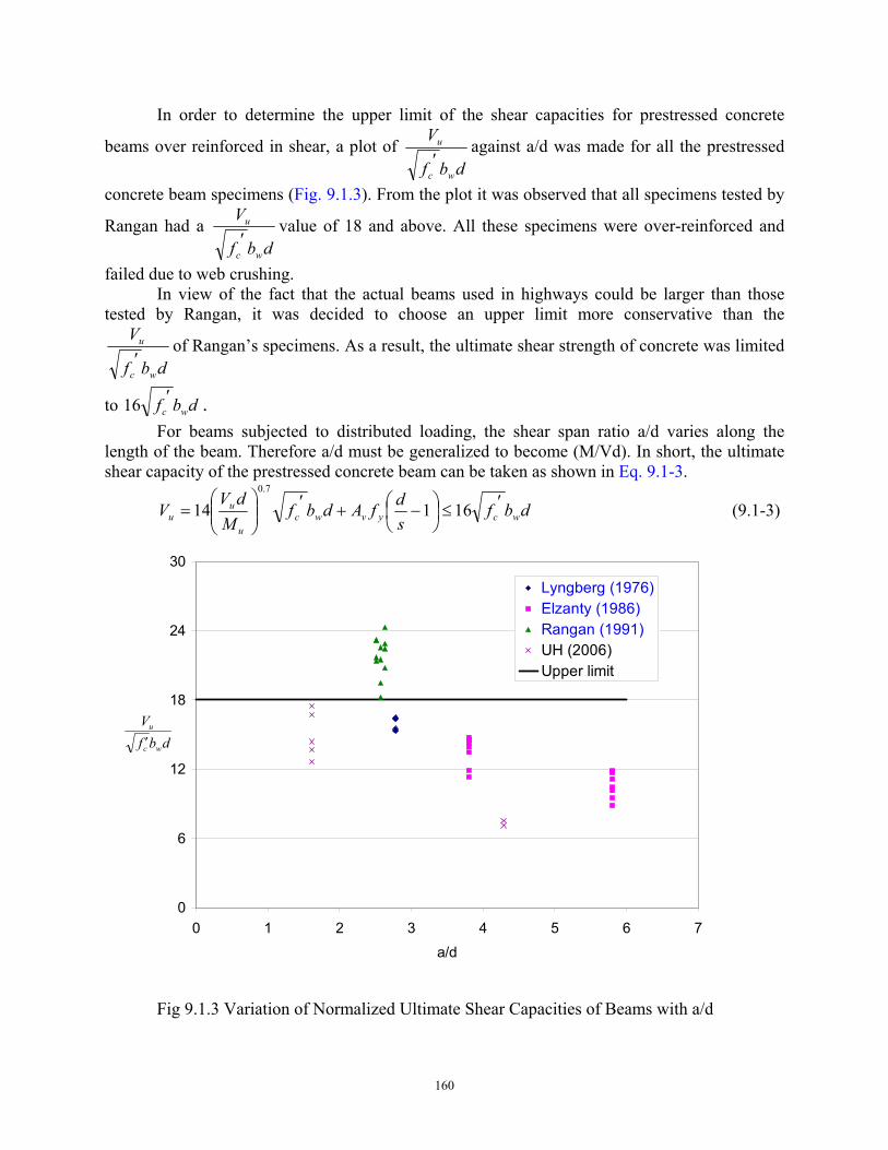
160

In order to determine the upper limit of the shear capacities for prestressed concrete

beams over reinforced in shear, a plot of dbf

V

wc

u

′against a/d was made for all the prestressed

concrete beam specimens (Fig. 9.1.3). From the plot it was observed that all specimens tested by

Rangan had a dbf

V

wc

u

′value of 18 and above. All these specimens were over-reinforced and

failed due to web crushing. In view of the fact that the actual beams used in highways could be larger than those

tested by Rangan, it was decided to choose an upper limit more conservative than the

dbf

V

wc

u

′of Rangan’s specimens. As a result, the ultimate shear strength of concrete was limited

to dbf wc′16 .

For beams subjected to distributed loading, the shear span ratio a/d varies along the length of the beam. Therefore a/d must be generalized to become (M/Vd). In short, the ultimate shear capacity of the prestressed concrete beam can be taken as shown in Eq. 9.1-3.

−+′

= 114

7.0

sdfAdbf

MdVV yvwcu

uu dbf wc

′≤16 (9.1-3)

Fig 9.1.3 Variation of Normalized Ultimate Shear Capacities of Beams with a/d

0

6

12

18

24

30

0 1 2 3 4 5 6 7a/d

Lyngberg (1976)Elzanty (1986)Rangan (1991)UH (2006)Upper limit

dbfV

wc

u

′

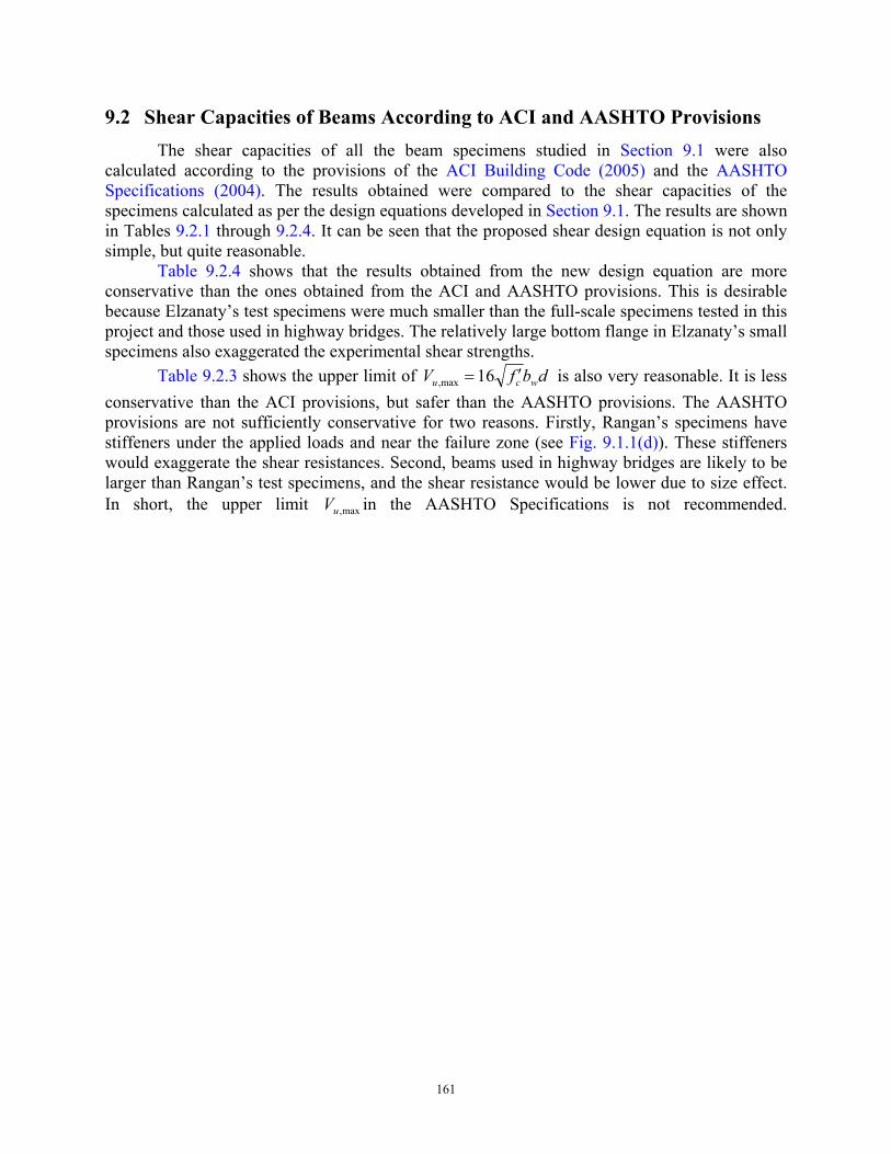
161

9.2 Shear Capacities of Beams According to ACI and AASHTO Provisions

The shear capacities of all the beam specimens studied in Section 9.1 were also calculated according to the provisions of the ACI Building Code (2005) and the AASHTO Specifications (2004). The results obtained were compared to the shear capacities of the specimens calculated as per the design equations developed in Section 9.1. The results are shown in Tables 9.2.1 through 9.2.4. It can be seen that the proposed shear design equation is not only simple, but quite reasonable.

Table 9.2.4 shows that the results obtained from the new design equation are more conservative than the ones obtained from the ACI and AASHTO provisions. This is desirable because Elzanaty’s test specimens were much smaller than the full-scale specimens tested in this project and those used in highway bridges. The relatively large bottom flange in Elzanaty’s small specimens also exaggerated the experimental shear strengths.

Table 9.2.3 shows the upper limit of dbfV wcu ′=16max, is also very reasonable. It is less conservative than the ACI provisions, but safer than the AASHTO provisions. The AASHTO provisions are not sufficiently conservative for two reasons. Firstly, Rangan’s specimens have stiffeners under the applied loads and near the failure zone (see Fig. 9.1.1(d)). These stiffeners would exaggerate the shear resistances. Second, beams used in highway bridges are likely to be larger than Rangan’s test specimens, and the shear resistance would be lower due to size effect. In short, the upper limit max,uV in the AASHTO Specifications is not recommended.

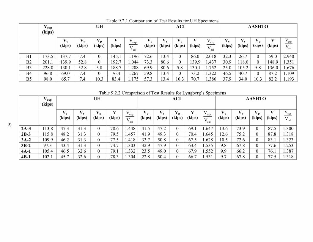
162

Table 9.2.1 Comparison of Test Results for UH Specimens UH ACI AASHTO Vexp

(kips)

Vc (kips)

Vs (kips)

Vp (kips)

V (kips)

cal

exp

VV

Vc

(kips)Vs

(kips)Vp

(kips) V

(kips) cal

exp

VV

Vc

(kips) Vs

(kips)Vp

(kips)V

(kips)cal

exp

VV

B1 173.5 137.7 7.4 0 145.1 1.196 72.6 13.4 0 86.0 2.018 32.3 26.7 0 59.0 2.940 B2 201.1 139.9 52.8 0 192.7 1.044 73.3 80.6 0 139.9 1.437 30.9 118.0 0 148.9 1.351 B3 228.0 130.1 52.8 5.8 188.7 1.208 69.9 80.6 5.8 130.1 1.752 25.0 105.2 5.8 136.0 1.676 B4 96.8 69.0 7.4 0 76.4 1.267 59.8 13.4 0 73.2 1.322 46.5 40.7 0 87.2 1.109 B5 98.0 65.7 7.4 10.3 83.4 1.175 57.3 13.4 10.3 70.7 1.386 37.9 34.0 10.3 82.2 1.193

Table 9.2.2 Comparison of Test Results for Lyngberg’s Specimens UH ACI AASHTO Vexp

(kips)

Vc (kips)

Vs (kips)

Vp (kips)

V (kips)

cal

exp

VV

Vc

(kips) Vs

(kips) Vp

(kips) V

(kips) cal

exp

VV

Vc

(kips) Vs

(kips) Vp

(kips)V

(kips)cal

exp

VV

2A-3 113.8 47.3 31.3 0 78.6 1.448 41.5 47.2 0 69.1 1.647 13.6 73.9 0 87.5 1.300 2B-3 115.8 48.2 31.3 0 79.5 1.457 41.9 49.3 0 70.4 1.645 12.6 75.2 0 87.8 1.318 3A-2 109.9 46.2 31.3 0 77.5 1.418 33.7 50.8 0 67.5 1.628 10.5 72.6 0 83.1 1.323 3B-2 97.3 43.4 31.3 0 74.7 1.303 32.9 47.9 0 63.4 1.535 9.8 67.8 0 77.6 1.253 4A-1 105.4 46.5 32.6 0 79.1 1.332 23.5 49.0 0 67.9 1.552 9.9 66.2 0 76.1 1.387 4B-1 102.1 45.7 32.6 0 78.3 1.304 22.8 50.4 0 66.7 1.531 9.7 67.8 0 77.5 1.318

162

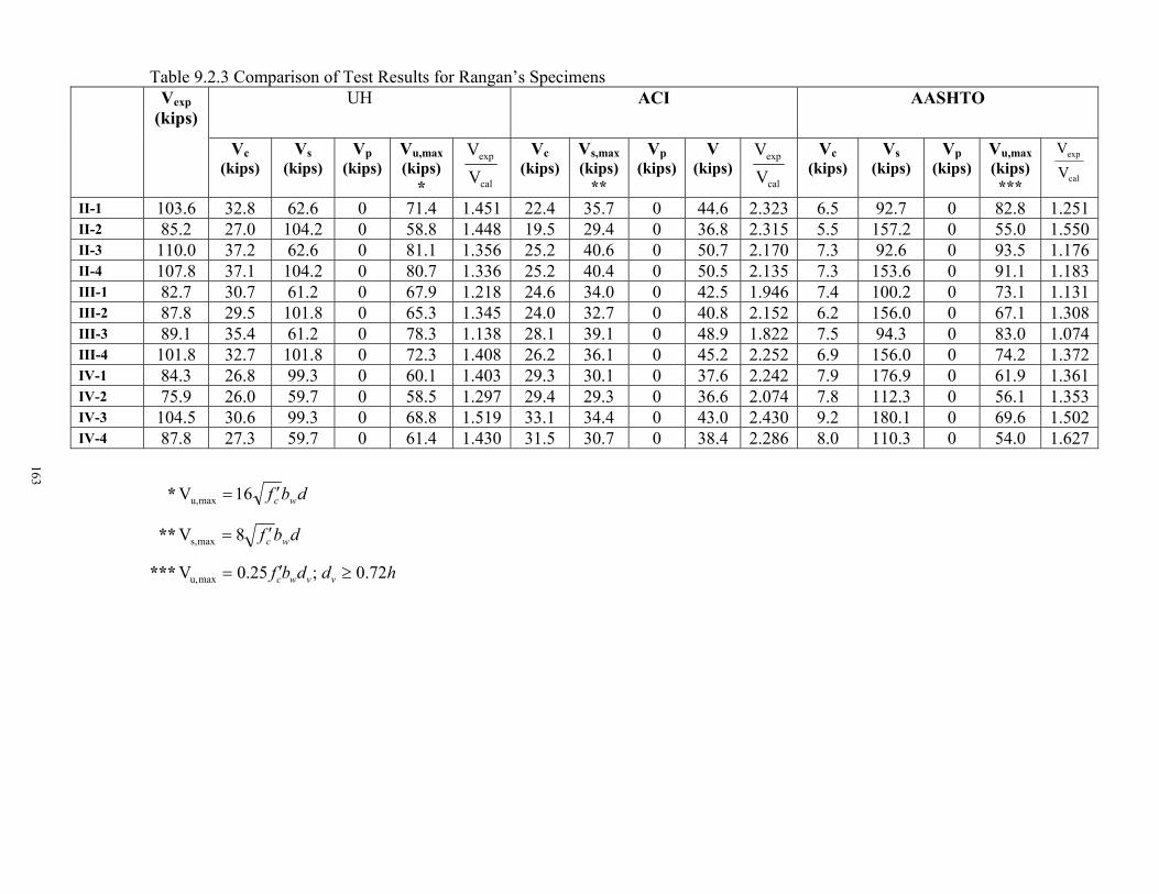
163

Table 9.2.3 Comparison of Test Results for Rangan’s Specimens UH ACI AASHTO Vexp

(kips)

Vc (kips)

Vs (kips)

Vp (kips)

Vu,max (kips)

* cal

exp

VV

Vc

(kips) Vs,max (kips)

**

Vp (kips)

V (kips)

cal

exp

VV

Vc

(kips) Vs

(kips) Vp

(kips)Vu,max (kips) *** cal

exp

VV

II-1 103.6 32.8 62.6 0 71.4 1.451 22.4 35.7 0 44.6 2.323 6.5 92.7 0 82.8 1.251 II-2 85.2 27.0 104.2 0 58.8 1.448 19.5 29.4 0 36.8 2.315 5.5 157.2 0 55.0 1.550 II-3 110.0 37.2 62.6 0 81.1 1.356 25.2 40.6 0 50.7 2.170 7.3 92.6 0 93.5 1.176 II-4 107.8 37.1 104.2 0 80.7 1.336 25.2 40.4 0 50.5 2.135 7.3 153.6 0 91.1 1.183 III-1 82.7 30.7 61.2 0 67.9 1.218 24.6 34.0 0 42.5 1.946 7.4 100.2 0 73.1 1.131 III-2 87.8 29.5 101.8 0 65.3 1.345 24.0 32.7 0 40.8 2.152 6.2 156.0 0 67.1 1.308 III-3 89.1 35.4 61.2 0 78.3 1.138 28.1 39.1 0 48.9 1.822 7.5 94.3 0 83.0 1.074 III-4 101.8 32.7 101.8 0 72.3 1.408 26.2 36.1 0 45.2 2.252 6.9 156.0 0 74.2 1.372 IV-1 84.3 26.8 99.3 0 60.1 1.403 29.3 30.1 0 37.6 2.242 7.9 176.9 0 61.9 1.361 IV-2 75.9 26.0 59.7 0 58.5 1.297 29.4 29.3 0 36.6 2.074 7.8 112.3 0 56.1 1.353 IV-3 104.5 30.6 99.3 0 68.8 1.519 33.1 34.4 0 43.0 2.430 9.2 180.1 0 69.6 1.502 IV-4 87.8 27.3 59.7 0 61.4 1.430 31.5 30.7 0 38.4 2.286 8.0 110.3 0 54.0 1.627

* dbf wc′=16V maxu,

** dbf wc′= 8V maxs,

*** hddbf vvwc 72.0;25.0V maxu, ≥′=

163

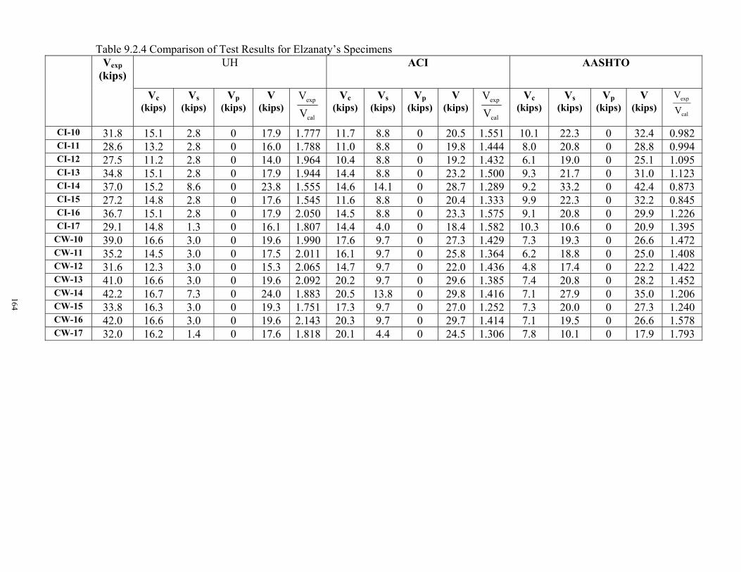
164

Table 9.2.4 Comparison of Test Results for Elzanaty’s Specimens UH ACI AASHTO Vexp

(kips)

Vc (kips)

Vs (kips)

Vp (kips)

V (kips)

cal

exp

VV

Vc

(kips) Vs

(kips) Vp

(kips) V

(kips) cal

exp

VV

Vc

(kips) Vs

(kips) Vp

(kips)V

(kips)cal

exp

VV

CI-10 31.8 15.1 2.8 0 17.9 1.777 11.7 8.8 0 20.5 1.551 10.1 22.3 0 32.4 0.982 CI-11 28.6 13.2 2.8 0 16.0 1.788 11.0 8.8 0 19.8 1.444 8.0 20.8 0 28.8 0.994 CI-12 27.5 11.2 2.8 0 14.0 1.964 10.4 8.8 0 19.2 1.432 6.1 19.0 0 25.1 1.095 CI-13 34.8 15.1 2.8 0 17.9 1.944 14.4 8.8 0 23.2 1.500 9.3 21.7 0 31.0 1.123 CI-14 37.0 15.2 8.6 0 23.8 1.555 14.6 14.1 0 28.7 1.289 9.2 33.2 0 42.4 0.873 CI-15 27.2 14.8 2.8 0 17.6 1.545 11.6 8.8 0 20.4 1.333 9.9 22.3 0 32.2 0.845 CI-16 36.7 15.1 2.8 0 17.9 2.050 14.5 8.8 0 23.3 1.575 9.1 20.8 0 29.9 1.226 CI-17 29.1 14.8 1.3 0 16.1 1.807 14.4 4.0 0 18.4 1.582 10.3 10.6 0 20.9 1.395

CW-10 39.0 16.6 3.0 0 19.6 1.990 17.6 9.7 0 27.3 1.429 7.3 19.3 0 26.6 1.472 CW-11 35.2 14.5 3.0 0 17.5 2.011 16.1 9.7 0 25.8 1.364 6.2 18.8 0 25.0 1.408 CW-12 31.6 12.3 3.0 0 15.3 2.065 14.7 9.7 0 22.0 1.436 4.8 17.4 0 22.2 1.422 CW-13 41.0 16.6 3.0 0 19.6 2.092 20.2 9.7 0 29.6 1.385 7.4 20.8 0 28.2 1.452 CW-14 42.2 16.7 7.3 0 24.0 1.883 20.5 13.8 0 29.8 1.416 7.1 27.9 0 35.0 1.206 CW-15 33.8 16.3 3.0 0 19.3 1.751 17.3 9.7 0 27.0 1.252 7.3 20.0 0 27.3 1.240 CW-16 42.0 16.6 3.0 0 19.6 2.143 20.3 9.7 0 29.7 1.414 7.1 19.5 0 26.6 1.578 CW-17 32.0 16.2 1.4 0 17.6 1.818 20.1 4.4 0 24.5 1.306 7.8 10.1 0 17.9 1.793

164

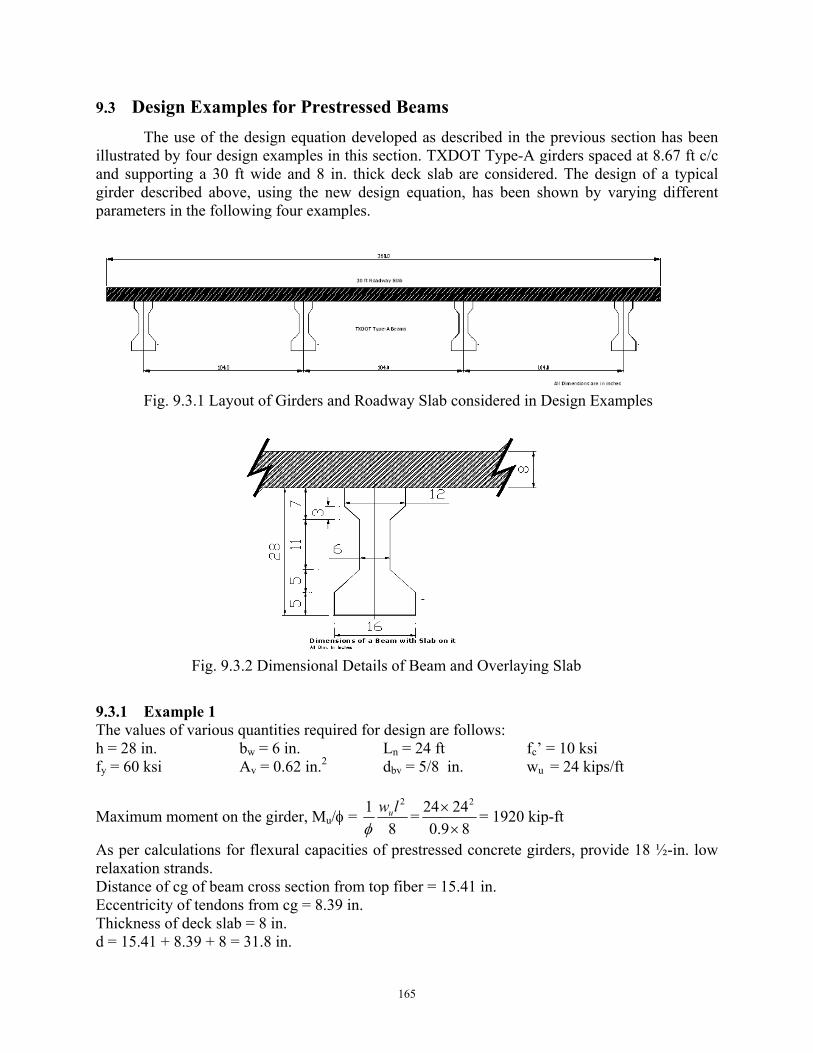
165

9.3 Design Examples for Prestressed Beams

The use of the design equation developed as described in the previous section has been illustrated by four design examples in this section. TXDOT Type-A girders spaced at 8.67 ft c/c and supporting a 30 ft wide and 8 in. thick deck slab are considered. The design of a typical girder described above, using the new design equation, has been shown by varying different parameters in the following four examples.

Fig. 9.3.1 Layout of Girders and Roadway Slab considered in Design Examples

Fig. 9.3.2 Dimensional Details of Beam and Overlaying Slab

9.3.1 Example 1 The values of various quantities required for design are follows: h = 28 in. bw = 6 in. Ln = 24 ft fc’ = 10 ksi fy = 60 ksi Av = 0.62 in.2 dbv = 5/8 in. wu = 24 kips/ft

Maximum moment on the girder, Mu/φ = 8

1 2lwu

φ=

89.02424 2

×× = 1920 kip-ft

As per calculations for flexural capacities of prestressed concrete girders, provide 18 ½-in. low relaxation strands. Distance of cg of beam cross section from top fiber = 15.41 in. Eccentricity of tendons from cg = 8.39 in. Thickness of deck slab = 8 in. d = 15.41 + 8.39 + 8 = 31.8 in.

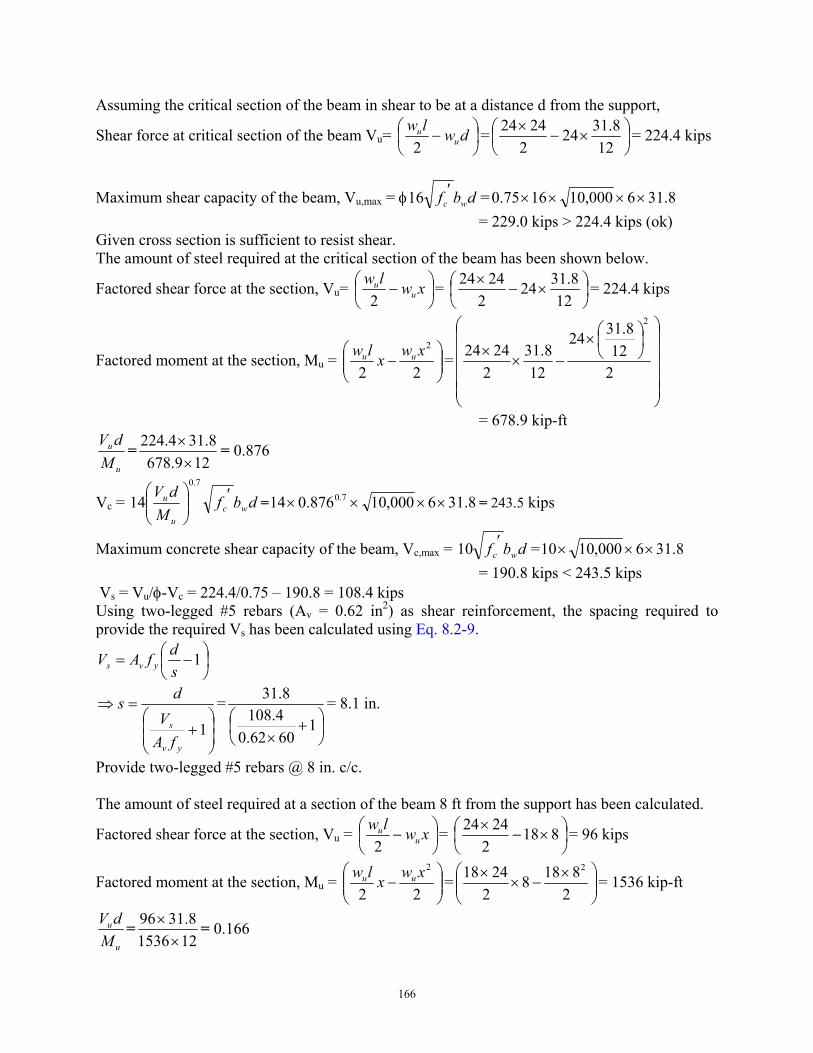
166

Assuming the critical section of the beam in shear to be at a distance d from the support,

Shear force at critical section of the beam Vu=

− dwlw

uu

2=

×−

×12

8.31242

2424 = 224.4 kips

Maximum shear capacity of the beam, Vu,max = φ dbf wc′16 = 8.316000,101675.0 ××××

= 229.0 kips > 224.4 kips (ok) Given cross section is sufficient to resist shear. The amount of steel required at the critical section of the beam has been shown below.

Factored shear force at the section, Vu=

− xwlw

uu

2=

×−

×12

8.31242

2424 = 224.4 kips

Factored moment at the section, Mu =

−

22

2xwxlw uu =

×

−××

212

8.3124

128.31

22424

2

= 678.9 kip-ft

u

u

MdV

=129.678

8.314.224×× = 0.876

Vc = dbfM

dVwc

u

u ′

7.0

14 = 8.316000,10876.014 7.0 ×××× = 243.5 kips

Maximum concrete shear capacity of the beam, Vc,max = dbf wc′10 = 8.316000,1010 ×××

= 190.8 kips < 243.5 kips Vs = Vu/φ-Vc = 224.4/0.75 – 190.8 = 108.4 kips Using two-legged #5 rebars (Av = 0.62 in2) as shear reinforcement, the spacing required to provide the required Vs has been calculated using Eq. 8.2-9.

−= 1

sdfAV yvs

+

=⇒

1yv

s

fAV

ds =

+

×1

6062.04.1088.31 = 8.1 in.

Provide two-legged #5 rebars @ 8 in. c/c. The amount of steel required at a section of the beam 8 ft from the support has been calculated.

Factored shear force at the section, Vu =

− xwlw

uu

2=

×−

× 8182

2424 = 96 kips


−

22

2xwxlw uu =

×−×

×2

81882

2418 2

= 1536 kip-ft

u

u

MdV =

1215368.3196

×× = 0.166

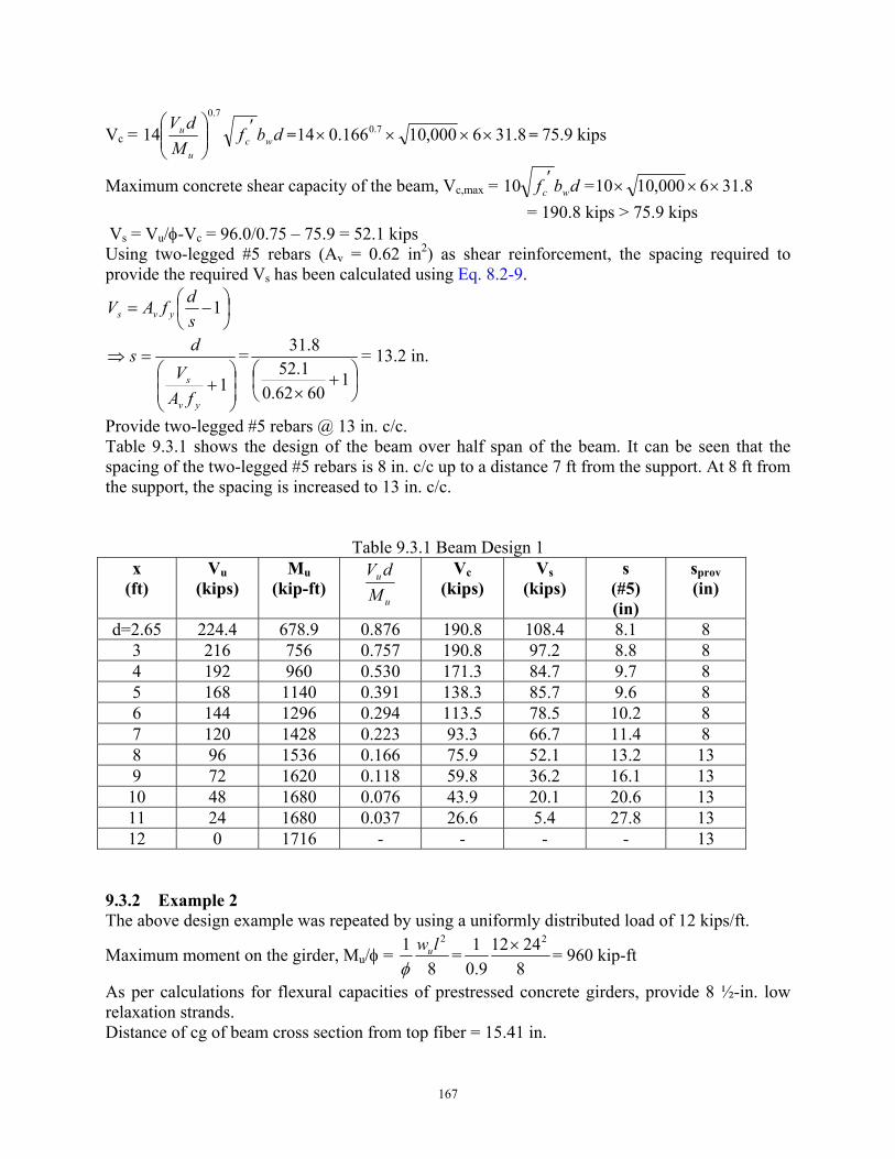
167

Vc = dbfM

dVwc

u

u ′

7.0

14 = 8.316000,10166.014 7.0 ×××× = 75.9 kips


= 190.8 kips > 75.9 kips Vs = Vu/φ-Vc = 96.0/0.75 – 75.9 = 52.1 kips Using two-legged #5 rebars (Av = 0.62 in2) as shear reinforcement, the spacing required to provide the required Vs has been calculated using Eq. 8.2-9.

−= 1

sdfAV yvs

+

=⇒

1yv

s

fAV

ds =

+

×1

6062.01.52

8.31 = 13.2 in.

Provide two-legged #5 rebars @ 13 in. c/c. Table 9.3.1 shows the design of the beam over half span of the beam. It can be seen that the spacing of the two-legged #5 rebars is 8 in. c/c up to a distance 7 ft from the support. At 8 ft from the support, the spacing is increased to 13 in. c/c.

Table 9.3.1 Beam Design 1 x

(ft) Vu

(kips) Mu

(kip-ft) u

u

MdV

Vc

(kips) Vs

(kips) s

(#5) (in)

sprov (in)

d=2.65 224.4 678.9 0.876 190.8 108.4 8.1 8 3 216 756 0.757 190.8 97.2 8.8 8 4 192 960 0.530 171.3 84.7 9.7 8 5 168 1140 0.391 138.3 85.7 9.6 8 6 144 1296 0.294 113.5 78.5 10.2 8 7 120 1428 0.223 93.3 66.7 11.4 8 8 96 1536 0.166 75.9 52.1 13.2 13 9 72 1620 0.118 59.8 36.2 16.1 13 10 48 1680 0.076 43.9 20.1 20.6 13 11 24 1680 0.037 26.6 5.4 27.8 13 12 0 1716 - - - - 13

9.3.2 Example 2 The above design example was repeated by using a uniformly distributed load of 12 kips/ft.


1 2lwu

φ=

82412

9.01 2× = 960 kip-ft

As per calculations for flexural capacities of prestressed concrete girders, provide 8 ½-in. low relaxation strands. Distance of cg of beam cross section from top fiber = 15.41 in.

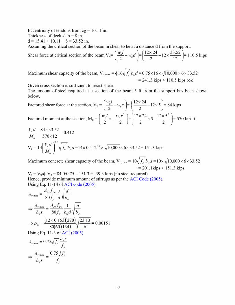
168

Eccentricity of tendons from cg = 10.11 in. Thickness of deck slab = 8 in. d = 15.41 + 10.11 + 8 = 33.52 in. Assuming the critical section of the beam in shear to be at a distance d from the support,


− dwlw

uu

2=

×−

×12

52.33122

2412 = 110.5 kips


= 241.3 kips > 110.5 kips (ok) Given cross section is sufficient to resist shear. The amount of steel required at a section of the beam 5 ft from the support has been shown below.


− xwlw

uu

2=

×−

× 5122

2412 = 84 kips


−

22

2xwxlw uu =

×−×

×2

51252

2412 2

= 570 kip-ft

u

u

MdV

=1257052.3384

×× = 0.412

Vc = dbfM

dVwc

u

u ′

7.0

14 = 52.336000,10412.014 7.0 ×××× = 151.3 kips


= 201.1kips > 151.3 kips Vs = Vu/φ-Vc = 84.0/0.75 – 151.3 = -39.3 kips (no steel required)

Hence, provide minimum amount of stirrups as per the ACI Code (2005). Using Eq. 11-14 of ACI code (2005)

wy

pupsv b

dds

ffA

A80min, =

wwy

pups

w

v

bd

dbffA

sbA 1

80min, =⇒

( )( )( )( ) 6

13.231346080

270153.012×=⇒ wρ = 0.00151

Using Eq. 11-3 of ACI (2005)

y

wcv f

sbfA ′= 75.0min,

y

c

w

v

ff

sbA ′

=⇒75.0min,

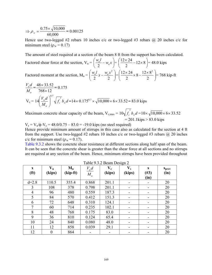
169

000,60000,1075.0 ×

=⇒ wρ = 0.00125

Hence use two-legged #2 rebars 10 inches c/c or two-legged #3 rebars @ 20 inches c/c for minimum steel (ρw = 0.17) The amount of steel required at a section of the beam 8 ft from the support has been calculated.


− xwlw

uu

2=

×−

× 8122

2412 = 48.0 kips


−

22

2xwxlw uu =

×−×

×2

81282

2412 2

= 768 kip-ft

u

u

MdV

=1276852.3348

×× = 0.175

Vc = dbfM

dVwc

u

u ′

7.0

14 = 52.336000,10175.014 7.0 ×××× = 83.0 kips


= 201.1kips > 83.0 kips Vs = Vu/φ-Vc = 48.0/0.75 – 83.0 = -19.0 kips (no steel required) Hence provide minimum amount of stirrups in this case also as calculated for the section at 4 ft from the support. Use two-legged #2 rebars 10 inches c/c or two-legged #3 rebars @ 20 inches c/c for minimum steel (ρw = 0.17). Table 9.3.2 shows the concrete shear resistance at different sections along half span of the beam. It can be seen that the concrete shear is greater than the shear force at all sections and no stirrups are required at any section of the beam. Hence, minimum stirrups have been provided throughout


(ft) Vu

(kips) Mu

(kip-ft) u

u

MdV

Vc

(kips) Vs

(kips) s

(#3) (in)

sprov (in)

d=2.8 110.5 355.4 0.868 201.1 - - 20 3 108 378 0.798 201.1 - - 20 4 96 480 0.559 187.3 - - 20 5 84 570 0.412 151.3 - - 20 6 72 648 0.310 124.1 - - 20 7 60 714 0.235 102.1 - - 20 8 48 768 0.175 83.0 - - 20 9 36 810 0.124 65.4 - - 20 10 24 840 0.080 48.0 - - 20 11 12 858 0.039 29.1 - - 20 12 0 864 - - - - 20

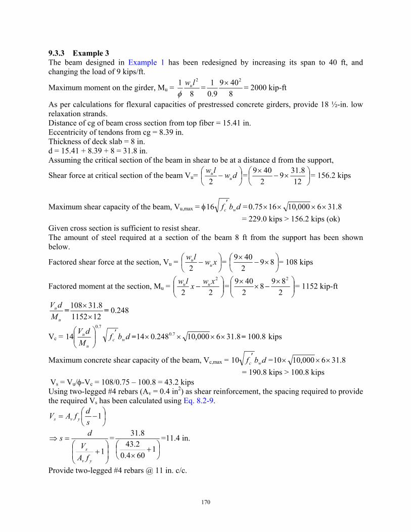
170

9.3.3 Example 3 The beam designed in Example 1 has been redesigned by increasing its span to 40 ft, and changing the load of 9 kips/ft.

Maximum moment on the girder, Mu = 8

1 2lwu

φ=

8409

9.01 2× = 2000 kip-ft

As per calculations for flexural capacities of prestressed concrete girders, provide 18 ½-in. low relaxation strands. Distance of cg of beam cross section from top fiber = 15.41 in. Eccentricity of tendons from cg = 8.39 in. Thickness of deck slab = 8 in. d = 15.41 + 8.39 + 8 = 31.8 in. Assuming the critical section of the beam in shear to be at a distance d from the support,


− dwlw

uu

2=

×−

×12

8.3192409 = 156.2 kips




− xwlw

uu

2=

×−

× 892409 = 108 kips


−

22

2xwxlw uu =

×−×

×2898

2409 2

= 1152 kip-ft

u

u

MdV

=121152

8.31108×

× = 0.248

Vc = dbfM

dVwc

u

u ′

7.0

14 = 8.316000,10248.014 7.0 ×××× = 100.8 kips


= 190.8 kips > 100.8 kips Vs = Vu/φ-Vc = 108/0.75 – 100.8 = 43.2 kips Using two-legged #4 rebars (Av = 0.4 in2) as shear reinforcement, the spacing required to provide the required Vs has been calculated using Eq. 8.2-9.

−= 1

sdfAV yvs

+

=⇒

1yv

s

fAV

ds =

+

×1

604.02.43

8.31 =11.4 in.

Provide two-legged #4 rebars @ 11 in. c/c.

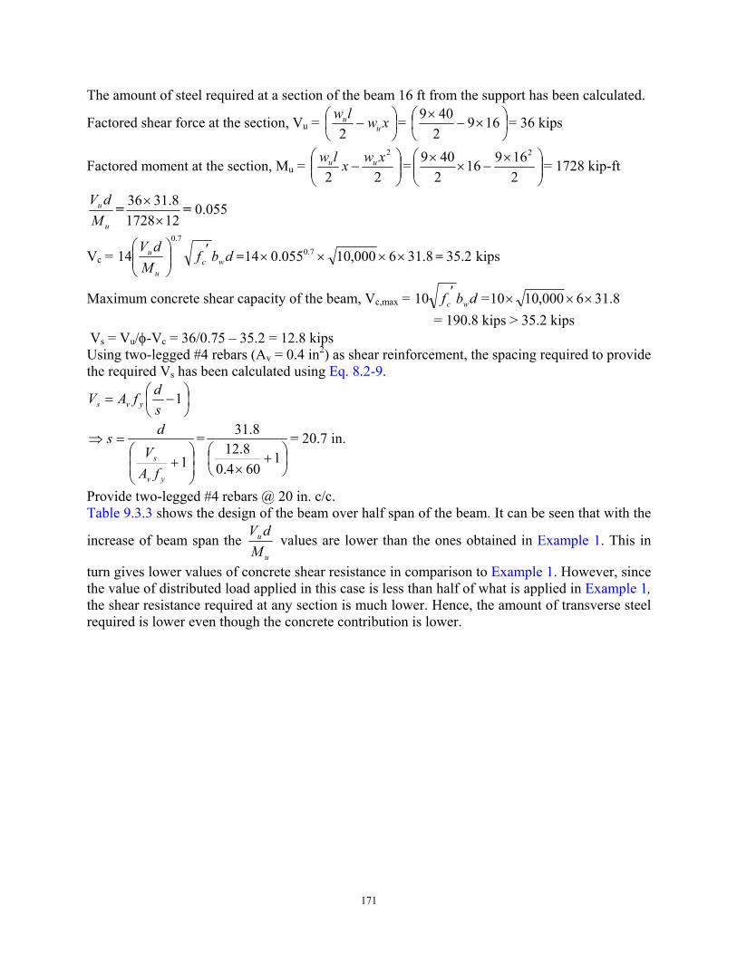
171

The amount of steel required at a section of the beam 16 ft from the support has been calculated.


− xwlw

uu

2=

×−

× 1692409 = 36 kips


−

22

2xwxlw uu =

×−×

×216916

2409 2

= 1728 kip-ft

u

u

MdV

=1217288.3136

×× = 0.055

Vc = dbfM

dVwc

u

u ′

7.0

14 = 8.316000,10055.014 7.0 ×××× = 35.2 kips


= 190.8 kips > 35.2 kips Vs = Vu/φ-Vc = 36/0.75 – 35.2 = 12.8 kips Using two-legged #4 rebars (Av = 0.4 in2) as shear reinforcement, the spacing required to provide the required Vs has been calculated using Eq. 8.2-9.

−= 1

sdfAV yvs

+

=⇒

1yv

s

fAV

ds =

+

×1

604.08.12

8.31 = 20.7 in.

Provide two-legged #4 rebars @ 20 in. c/c. Table 9.3.3 shows the design of the beam over half span of the beam. It can be seen that with the

increase of beam span the u

u

MdV

values are lower than the ones obtained in Example 1. This in

turn gives lower values of concrete shear resistance in comparison to Example 1. However, since the value of distributed load applied in this case is less than half of what is applied in Example 1, the shear resistance required at any section is much lower. Hence, the amount of transverse steel required is lower even though the concrete contribution is lower.

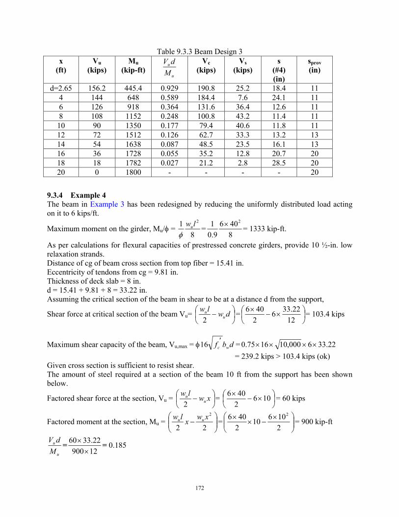
172


(ft) Vu

(kips) Mu

(kip-ft) u

u

MdV

Vc

(kips) Vs

(kips) s

(#4) (in)

sprov (in)

d=2.65 156.2 445.4 0.929 190.8 25.2 18.4 11 4 144 648 0.589 184.4 7.6 24.1 11 6 126 918 0.364 131.6 36.4 12.6 11 8 108 1152 0.248 100.8 43.2 11.4 11 10 90 1350 0.177 79.4 40.6 11.8 11 12 72 1512 0.126 62.7 33.3 13.2 13 14 54 1638 0.087 48.5 23.5 16.1 13 16 36 1728 0.055 35.2 12.8 20.7 20 18 18 1782 0.027 21.2 2.8 28.5 20 20 0 1800 - - - - 20

9.3.4 Example 4 The beam in Example 3 has been redesigned by reducing the uniformly distributed load acting on it to 6 kips/ft.


1 2lwu

φ=

8406

9.01 2× = 1333 kip-ft.

As per calculations for flexural capacities of prestressed concrete girders, provide 10 ½-in. low relaxation strands. Distance of cg of beam cross section from top fiber = 15.41 in. Eccentricity of tendons from cg = 9.81 in. Thickness of deck slab = 8 in. d = 15.41 + 9.81 + 8 = 33.22 in. Assuming the critical section of the beam in shear to be at a distance d from the support,


− dwlw

uu

2=

×−

×12

22.3362406 = 103.4 kips




− xwlw

uu

2=

×−

× 1062406 = 60 kips


−

22

2xwxlw uu =

×−×

×210610

2406 2

= 900 kip-ft

u

u

MdV

=1290022.3360

×× = 0.185

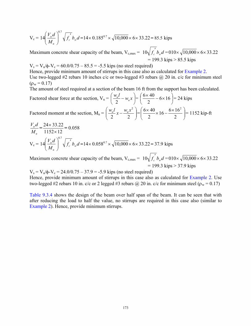
173

Vc = dbfM

dVwc

u

u ′

7.0

14 = 22.336000,10185.014 7.0 ×××× = 85.5 kips


= 199.3 kips > 85.5 kips Vs = Vu/φ-Vc = 60.0/0.75 – 85.5 = -5.5 kips (no steel required) Hence, provide minimum amount of stirrups in this case also as calculated for Example 2. Use two-legged #2 rebars 10 inches c/c or two-legged #3 rebars @ 20 in. c/c for minimum steel (ρw = 0.17) The amount of steel required at a section of the beam 16 ft from the support has been calculated.


− xwlw

uu

2=

×−

× 1662406 = 24 kips


−

22

2xwxlw uu =

×−×

×216616

2406 2

= 1152 kip-ft

u

u

MdV

=12115222.3324

×× = 0.058

Vc = dbfM

dVwc

u

u ′

7.0

14 = 22.336000,10058.014 7.0 ×××× = 37.9 kips


= 199.3 kips > 37.9 kips Vs = Vu/φ-Vc = 24.0/0.75 – 37.9 = -5.9 kips (no steel required) Hence, provide minimum amount of stirrups in this case also as calculated for Example 2. Use two-legged #2 rebars 10 in. c/c or 2 legged #3 rebars @ 20 in. c/c for minimum steel (ρw = 0.17) Table 9.3.4 shows the design of the beam over half span of the beam. It can be seen that with after reducing the load to half the value, no stirrups are required in this case also (similar to Example 2). Hence, provide minimum stirrups.

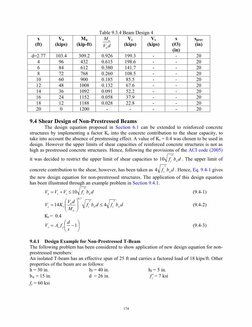
174


(ft) Vu

(kips) Mu

(kip-ft) dVM

u

u Vc (kips)

Vs (kips)

s (#3) (in)

sprov (in)

d=2.77 103.4 309.2 0.926 199.3 - - 20 4 96 432 0.615 198.6 - - 20 6 84 612 0.380 141.7 - - 20 8 72 768 0.260 108.5 - - 20 10 60 900 0.185 85.5 - - 20 12 48 1008 0.132 67.6 - - 20 14 36 1092 0.091 52.2 - - 20 16 24 1152 0.058 37.9 - - 20 18 12 1188 0.028 22.8 - - 20 20 0 1200 - - - - 20

9.4 Shear Design of Non-Prestressed Beams

The design equation proposed in Section 6.1 can be extended to reinforced concrete structures by implementing a factor Kr into the concrete contribution to the shear capacity, to take into account the absence of prestressing effect. A value of Kr = 0.4 was chosen to be used in design. However the upper limits of shear capacities of reinforced concrete structures is not as high as prestressed concrete structures. Hence, following the provisions of the ACI code (2005)

it was decided to restrict the upper limit of shear capacities to dbf wc′10 . The upper limit of

concrete contribution to the shear, however, has been taken as dbf wc′4 . Hence, Eq. 9.4-1 gives

the new design equation for non-prestressed structures. The application of this design equation has been illustrated through an example problem in Section 9.4.1.

scu VVV += dbf wc′≤10 (9.4-1)

dbfM

dVKV wcu

urc

′

=

7.0

14 dbf wc′≤ 4 (9.4-2)

Kr = 0.4

−= 1

sdfAV yvs (9.4-3)

9.4.1 Design Example for Non-Prestressed T-Beam The following problem has been considered to show application of new design equation for non-prestressed members: An isolated T-beam has an effective span of 25 ft and carries a factored load of 18 kips/ft. Other properties of the beam are as follows: h = 30 in. bf = 40 in. hf = 5 in. bw = 15 in. d = 26 in. cf ′= 7 ksi fy = 60 ksi

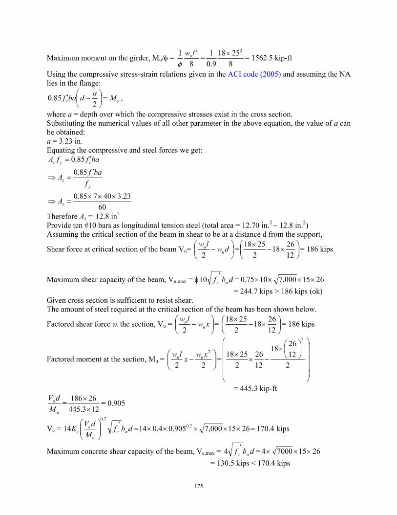
175


1 2lwu

φ=

82518

9.01 2× = 1562.5 kip-ft

Using the compressive stress-strain relations given in the ACI code (2005) and assuming the NA lies in the flange:

uc Madbaf =

−′

285.0 ,

where a = depth over which the compressive stresses exist in the cross section. Substituting the numerical values of all other parameter in the above equation, the value of a can be obtained: a = 3.23 in. Equating the compressive and steel forces we get:

6023.340785.0

85.0

85.0

×××=⇒

′=⇒

′=

s

y

cs

cys

A

fbafA

baffA

Therefore As = 12.8 in2 Provide ten #10 bars as longitudinal tension steel (total area = 12.70 in.2 ~ 12.8 in.2) Assuming the critical section of the beam in shear to be at a distance d from the support,


− dwlw

uu

2=

×−

×122618

22518 = 186 kips

Maximum shear capacity of the beam, Vu,max = φ dbf wc′10 = 2615000,71075.0 ××××

= 244.7 kips > 186 kips (ok) Given cross section is sufficient to resist shear. The amount of steel required at the critical section of the beam has been shown below.


− xwlw

uu

2=

×−

×122618

22518 = 186 kips


−

22

2xwxlw uu =

×

−××

2122618

1226

22518

2

= 445.3 kip-ft

u

u

MdV

=123.445

26186×× = 0.905

Vc = dbfM

dVK wcu

ur

′

7.0

14 = 2615000,7905.04.014 7.0 ××××× = 170.4 kips

Maximum concrete shear capacity of the beam, Vc,max = dbf wc′4 = 261570004 ×××

= 130.5 kips < 170.4 kips

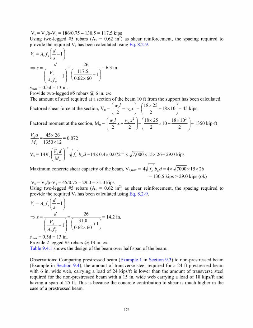
176

Vs = Vu/φ-Vc = 186/0.75 – 130.5 = 117.5 kips Using two-legged #5 rebars (Av = 0.62 in2) as shear reinforcement, the spacing required to provide the required Vs has been calculated using Eq. 8.2-9.

−= 1

sdfAV yvs

+

=⇒

1yv

s

fAV

ds =

+

×1

6062.05.117

26 = 6.3 in.

smax = 0.5d = 13 in. Provide two-legged #5 rebars @ 6 in. c/c The amount of steel required at a section of the beam 10 ft from the support has been calculated.


− xwlw

uu

2=

×−

× 10182

2518 = 45 kips


−

22

2xwxlw uu =

×−×

×2101810

22518 2

= 1350 kip-ft

u

u

MdV

=121350

2645×× = 0.072

Vc = dbfM

dVK wcu

ur

′

7.0

14 = 2615000,7072.04.014 7.0 ××××× = 29.0 kips


= 130.5 kips > 29.0 kips (ok) Vs = Vu/φ-Vc = 45/0.75 – 29.0 = 31.0 kips Using two-legged #5 rebars (Av = 0.62 in2) as shear reinforcement, the spacing required to provide the required Vs has been calculated using Eq. 8.2-9.

−= 1

sdfAV yvs

+

=⇒

1yv

s

fAV

ds =

+

×1

6062.00.3126 = 14.2 in.

smax = 0.5d = 13 in. Provide 2 legged #5 rebars @ 13 in. c/c. Table 9.4.1 shows the design of the beam over half span of the beam. Observations: Comparing prestressed beam (Example 1 in Section 9.3) to non-prestressed beam (Example in Section 9.4), the amount of transverse steel required for a 24 ft prestressed beam with 6 in. wide web, carrying a load of 24 kips/ft is lower than the amount of transverse steel required for the non-prestressed beam with a 15 in. wide web carrying a load of 18 kips/ft and having a span of 25 ft. This is because the concrete contribution to shear is much higher in the case of a prestressed beam.

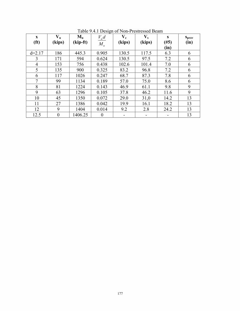
177

Table 9.4.1 Design of Non-Prestressed Beam x

(ft) Vu

(kips) Mu

(kip-ft) u

u

MdV

Vc

(kips) Vs

(kips) s

(#5) (in)

sprov (in)

d=2.17 186 445.3 0.905 130.5 117.5 6.3 6 3 171 594 0.624 130.5 97.5 7.2 6 4 153 756 0.438 102.6 101.4 7.0 6 5 135 900 0.325 83.2 96.8 7.2 6 6 117 1026 0.247 68.7 87.3 7.8 6 7 99 1134 0.189 57.0 75.0 8.6 6 8 81 1224 0.143 46.9 61.1 9.8 9 9 63 1296 0.105 37.8 46.2 11.6 9 10 45 1350 0.072 29.0 31,0 14.2 13 11 27 1386 0.042 19.9 16.1 18.2 13 12 9 1404 0.014 9.2 2.8 24.2 13

12.5 0 1406.25 0 - - - 13

179

CHAPTER 10

CONCLUSIONS AND SUGGESTIONS

10.1 Conclusions The purpose of this research is to study the behavior of prestressed concrete elements and

beams under shear and to finally develop a simplified equation for the shear design of prestressed concrete girders. The following conclusions are made from this research:

(1) The Softened Membrane Model for Prestressed Concrete (SMM-PC) is presented in this research as an analytical model to predict shear behavior of prestressed concrete elements. The SMM-PC is an extension of the SMM developed at the University of Houston (Hsu and Zhu, 2002; Zhu, 2000; Zhu and Hsu, 2002). This new model is applicable to reinforced and prestressed concrete, with any ratio of longitudinal steel to transverse steel, and in any orientation of steel reinforcement with respect to the applied principal stresses. Although this model was verified for application to concrete of normal strength (42 MPa) in this research project, future research is likely to prove that it is also applicable to high-strength concrete up to 100 MPa.

(2) To implement the new model SMM-PC, new constitutive laws are established for prestressed concrete under sequential and proportional loading. The constitutive laws of concrete in tension include the decompression load stage.

(3) Prestress causes a 15% increase of concrete compressive strength under sequential loading. In the case of proportional loading, a prestress factor Wp is proposed for incorporation into the softening coefficient of prestressed concrete. Wp is expressed in terms of the deviation angle β, and takes care of the effect of prestress on concrete compressive strength.

(4) The constitutive laws of prestressing strands embedded in concrete are obtained. Compared to bare prestressing strands, the smeared (average) stress-strain relationships of prestressing strands has a lower ultimate strength, a lower elastic limit, and a knee region of smaller curvature.

(5) A post-tensioning system was developed for seven-wire strands to simulate the bond condition of pre-tensioning strands. A system of self-compacting concrete grout (SCCG) in flexible conduits was developed to create the same crack patterns in post-tensioned concrete as those in pre-tensioned concrete.

(6) The shear behavior of prestressed concrete beams was critically examined by full-scale tests on five TXDOT Type-A beams with web shear or flexural shear failure

(7) Using the constitutive laws developed in this research, an analytical model is developed to calculate the ultimate shear capacity of the prestressed concrete beams. Using this model, ultimate capacities of beams can be calculated corresponding to given angles of failure planes.

(8) A new design equation is developed using the results of the beam tests performed in this research as well as test results from other tests available in literature. Four design examples are shown to illustrate the use of the developed design equation for prestressed girders.

180

(9) The new design equation is extended to include non-prestressed girders, and a design example for the same is also prepared.

10.2 Suggestions Future research in this area are suggested as follows: (1) Whereas the prestressed concrete panels were subjected to pure shear in this research,

future research is desired to study the effect of normal stresses on the shear strength of elements. The Universal Panel Tester can be used to apply a combination of normal and shear stresses to prestressed concrete panels.

(2) Because high-strength concrete is widely used in prestressed concrete construction, the application of the SMM-PC model to high-strength prestressed concrete elements needs to be validated.

(3) Finite element programs should be developed based on the SMM-PC model to predict the behavior of whole prestressed concrete structures.

181

REFERENCES

AASHTO (2004), “AASHTO LRFD Bridge Design Specifications,” 1998, (also 1999 and 2000 Interim Revisions), American Association of State Highway and Transportation Officials (AASHTO), Washington, D. C.

ACI Committee 318 (2005), “Building Code Requirements for Structural Concrete (ACI 318-02) and Commentary (ACI 318R-02),” American Concrete Institute, Farmington Hills, MI.

Ayoub, Amir and Filippou, Filip C. (1998), “Nonlinear Finite-Element Analysis of RC Shear Panels and Walls,” Journal of Structural Engineering, ASCE, Vol. 124, No. 3, Mar. 1998, pp. 298-308.

Balakrishnan, S. and Murray, D. W. (1988a), “Concrete Constitutive Model for NLFE Analysis of Structures,” Journal of Structural Engineering, ASCE, Vol. 114, No. 7, July 1988, pp. 1449-1466.

Balakrishnan, S. and Murray, D. W. (1988b), “Strength of Reinforced Concrete Panels,” Canadian Journal of Civil Engineering, Vol. 15, No. 5, Oct. 1988, pp. 900-911.

Balakrishnan, S. and Murray, D. W. (1988c), “Prediction of R/C Panels and Deep Beam Behavior by NLFEA,” Journal of Structural Engineering, ASCE, Vol. 114, No. 10, Oct. 1988, pp. 2323-2342.

Belarbi, A. and Hsu, T. T. C. (1994), “Constitutive Laws of Concrete in Tension and Reinforcing Bars Stiffened by Concrete,” Structural Journal of the American Concrete Institute, Vol. 91, No. 4, pp. 465-474.

Belarbi, A. and Hsu, T. T. C. (1995), “Constitutive Laws of Softened Concrete in Biaxial Tension-Compression,” Structural Journal of the American Concrete Institute, Vol. 92, No. 5, pp. 562-573.

Belletti, B., Cerioni, R., and Iori, I. (2001), “Physical Approach for Reinforced-Concrete (PARC) Membrane Elements,” Journal of Structural Engineering, ASCE, Vol. 127, No. 12, Dec. 2001, pp. 1412-1426.

Bhide, B. S. and Collins, M. P. (1989), “Influence of Axial Tension on Shear Capacity of Reinforced Concrete Members,” ACI Structural Journal, Vol. 86, No. 5, pp. 570-580.

Carreira, D. J. and Chu, K. H. (1986), “Stress-Strain Relationship of Reinforced Concrete in Tension,” Journal of the American Concrete Institute, Vol. 83, No. 1, Jan.-Feb. 1986, pp. 21-28.

Chintrakarn, R. (2001), “Minimum Shear Steel and Failure Modes Diagram of Reinforced Concrete Membrane Elements,” Master’s Thesis, Department of Civil and Environmental Engineering, University of Houston, Houston, TX.

Collins, M. P., Vecchio, F. J., and Mehlhorn, G. (1985), “An International Competition to Predict the Response of Reinforced Concrete Panels,” Canadian Journal of Civil Engineering, Ottawa, Vol. 12, No. 3, pp. 626-644.

Crisfield, Michael A. and Wills, John (1989), “Analysis of R/C Panels Using Different Concrete Models,” Journal of Engineering Mechanics, ASCE, Vol. 115, No. 3, Mar. 1989, pp. 578-597.

182

Elzanaty, Ashraf H., Nilson, Arthur H., and Slate, Floyd O. (1986), “Shear Capacity of Prestressed Concrete Beams Using High Strength Concrete,” ACI Journal, Vol. 83, No. 3, May-June 1986, pp. 359-368.

Fenves, G. L. (2001), “Annual Workshop on Open System for Earthquake Engineering Simulation,” Pacific Earthquake Engineering Research Center, UC Berkeley, http://opensees.berkeley.edu/.

Foster, Stephen J. and Marti, Peter (2003), “Cracked Membrane Model: Finite Element Implementation,” Journal of Structural Engineering, ASCE, Vol. 129, No. 9, Sept. 2003, pp. 1155-1163.

Freyssinet, E. (1956), “The Birth of Prestressing,” Cement and Concrete Association Translation No. 29, London.

Gere, James M. and Timoshenko, Stephen P. (1991), Mechanics of Materials, Chapman and Hall, London, UK, 807 pp.

Hsu, T. T. C. (1993), Unified Theory of Reinforced Concrete, CRC Press, Inc., Boca Raton, FL, 336 pp.

Hsu, T. T. C. (1998), “Stresses and Crack Angles in Concrete Membrane Elements,” Journal of Structural Engineering, ASCE, Vol. 124, No. 12, Dec. 1998, pp. 1476-1484.

Hsu, T. T. C. (2002), “Rational Shear Design of Reinforced Concrete Bridges,” Presented at ACI 343/445 Session “Concrete Bridges in Shear,” ACI Fall Convention, Phoenix, AZ, Oct. 27 – Nov. 1, 2002.

Hsu, T. T. C., Belarbi, A., and Pang, X. B. (1995), “A Universal Panel Tester,” Journal of Testing and Evaluations, ASTM, Vol. 23, No. 1, pp. 41-49.

Hsu, T. T. C. and Zhang, L. X. (1996), “Tension Stiffening in Reinforced Concrete Membrane Elements,” Structural Journal of the American Concrete Institute, Vol. 93, No. 1, pp. 108-115.

Hsu, T. T. C. and Zhang, L. X. (1997), “Nonlinear Analysis of Membrane Elements by Fixed-Angle Softened-Truss Model,” Structural Journal of the American Concrete Institute, Vol. 94, No. 5, pp. 483-492.

Hsu, T. T. C. and Zhu, R. R. H. (2002), “Softened Membrane Model for Reinforced Concrete Elements in Shear,” Structural Journal of the American Concrete Institute, Vol. 99, No. 4, pp. 460-469.

Kaufmann, Walter and Marti, Peter (1998), “Structural Concrete: Cracked Membrane Model,” Journal of Structural Engineering, Vol. 124, No. 12, Dec. 1998, pp. 1467-1475.

Loov, R. E. (1978), “Design of Precast Connections,” Paper presented at a seminar organized by Compa International Pte, Ltd., September 25-27, Singapore, pp. 8.

Loov, R. E. (1997), “The Direct Computation of Stirrup Spacing Based on Shear-Friction,” Symposium on Advanced Design of Concrete Structures, Chalmers University of Technology, Goteborg, June 12-14.

Loov, R. E. (2002), “Shear Design of Uniformly Loaded Beams,” Presented at the Sixth International Conference on Short and Medium Span Bridges, Vancouver, Canada, July 31 – August 2, 2002.

http://opensees.berkeley.edu/

183

Lyngberg, Bent S. (1976), “Ultimate Shear Resistance of Partially Prestressed Reinforced Concrete I-Beams,” ACI Journal, Vol. 73, No. 4, April 1976, pp. 214-222.

Mansour, M. (2001), “Behavior of Reinforced Concrete Membrane Elements under Cyclic Shear: Experiments to Theory,” Ph.D. Dissertation, Department of Civil and Environmental Engineering, University of Houston, Houston, TX.

Mansour, M. and Hsu, T. T. C. (2005a), “Behavior of Reinforced Concrete Elements under Cyclic Shear: Part 1 – Experiments,” Journal of Structural Engineering, ASCE, Vol. 131, No. 1, January, 2005, pp. 44-53.

Mansour, M. and Hsu, T. T. C. (2005b), “Behavior of Reinforced Concrete Elements under Cyclic Shear: Part 2-Theoretical Model,” Journal of Structural Engineering, ASCE, Vol. 131, No. 1, January 2005, pp. 54-65.

Marti, P. and Meyboom, J. (1992), “Response of Prestressed Concrete Elements to In-plane Shear Forces,” ACI Structural Journal, Vol. 89, No. 5, Sept.-Oct. 1992, pp. 503-514.

Meyboom, J. (1987), “An Experimental Investigation of Partially Prestressed, Orthogonally Reinforced Concrete Elements Subjected to Membrane Shear,” Thesis, Department of Civil Engineering, University of Toronto, Toronto, Canada.

Morsch, E. (1902), “Der Eisenbetonbau, seine Anwendung und Theorie,” Wayss and Freytag, A.G., Im Selbstverlag der Firma, Neustadt, A.D. Haardt, May 1902, pp. 118.

Nawy, E. G. (1985), Reinforced Concrete: A Fundamental Approach, Prentice-Hall Press, Inc., Englewood Cliffs, NJ, 701 pp.

Pang, X. B. (1991), “Constitutive Laws of Reinforced Concrete in Shear,” Ph.D. Dissertation, Department of Civil and Environmental Engineering, University of Houston, Houston, TX.

Pang, X. B. and Hsu, T. T. C. (1995), “Behavior of Reinforced Concrete Membrane Elements in Shear,” Structural Journal of the American Concrete Institute, Vol. 92, No. 6, pp. 665-679.

Pang, X. B. and Hsu, T. T. C. (1996), “Fixed-Angle Softened-Truss Model for Reinforced Concrete,” Structural Journal of the American Concrete Institute, Vol. 93, No. 2, pp. 197-207.

Rahal, K. N. (2002), “Membrane Elements Subjected to In-plane Shearing and Normal Stresses,” Journal of Structural Engineering, ASCE, Vol. 128, No. 8, August 2002, pp. 1064-1072.

Rangan, B. Vijaya (1991), “Web Crushing Strength of Reinforced and Prestressed Concrete Beams,” ACI Structural Journal, Vol. 88, No. 1, Jan.-Feb. 1991, pp. 12-16.

Ritter, W. (1899), “ Die Bauweise Hennebique,” Schweizerische Bauzeitung, Vol.33, No. 5, 6, and 7, Zurich, pp. 41-43, 49-52, and 59-61.

Robinson, J. R. and Demorieux, J. M. (1968), “Essai de Traction-Compression sur Modeles d’Ames de Poutre en Beton Arme,” Compte Rendu Partiel I, U.T.I., Institut de Recherches Appliquees du Beton Arme, Paris, France, 43 pp.

Tamai, S., Shima, H., Izumo, J., and Okamura, H. (1987), “Average Stress-Strain Relationship in Post Yield Range of Steel Bar in Concrete,” Concrete Library of JSCE, No. 11, June 1988, pp.117-129. (Translating from Proceeding of JSCE, No. 378/V-6, Feb. 1987.)

Vecchio, F. J. (1990), “Reinforced Concrete Membrane Element Formulation,” Journal of Structural Engineering, ASCE, Vol. 116, No. 3, pp. 730-750.

184

Vecchio, F. J. (2000), “Disturbed Stress Field Model for Reinforced Concrete: Formulation,” Journal of Structural Engineering, ASCE, Vol. 126, No. 9, Sept. 2000, pp. 1070-1077.

Vecchio, F. J. (2001a), “Disturbed Stress Field Model for Reinforced Concrete: Implementation,” Journal of Structural Engineering, ASCE, Vol. 127, No. 1, Jan. 2001, pp. 12-20.

Vecchio, F. J. and Collins, M. P. (1981), “Stress-Strain Characteristic of Reinforced Concrete in Pure Shear,” IABSE Colloquium, Advanced Mechanics of Reinforced Concrete, Delft, Final Report, International Association of Bridge and Structural Engineering, Zurich, Switzerland, pp. 221-225.

Vecchio, F. J. and Collins, M. P. (1982), “Response of Reinforced Concrete to In Plane Shear and Normal Stresses,” Report, No. 82-03, University of Toronto, Toronto, Canada.

Vecchio, F. J. and Collins, M. P. (1986), “The Modified Compression Field Theory for Reinforced Concrete Elements Subjected to Shear,” ACI Journal, Vol. 83, No. 2, pp. 219-231.

Vecchio, F. J., Lai, D., Sim, W., and Ng, J. (2001), “Disturbed Stress Field Model for Reinforced Concrete: Validation,” Journal of Structural Engineering, ASCE, Vol. 127, No. 4, April 2001, pp. 350-358.

Wang, J. (2006), “Constitutive Relationships of Prestressed Concrete Membrane Elements,” Ph.D. Dissertation, Department of Civil and Environmental Engineering, University of Houston, Houston, TX.

Zhang, L. X. (1992), “Constitutive Laws of Reinforced Elements with Medium-High Strength Concrete,” Ph.D. Dissertation, Department of Civil and Environmental Engineering, University of Houston, Houston, TX.

Zhang, L. X. and Hsu, T. T. C. (1998), “Behavior and Analysis of 100Mpa Concrete Membrane Elements,” Journal of Structural Engineering, ASCE, Vol. 124, No. 1, Jan. 1998, pp. 24-34.

Zhong, J. X. (2005), “Model-Based Simulation of Reinforced Concrete Plane Stress Structures,” Ph.D. Dissertation, Department of Civil and Environmental Engineering, University of Houston, Houston, TX.

Zhu, R. R. H. (2000), “Softened-Membrane Model for Cracked Reinforced Concrete Considering Poisson Effect,” Ph.D. Dissertation, Department of Civil and Environmental Engineering, University of Houston, Houston, TX.

Zhu, R. H., Hsu, T. T. C., and Lee, J. Y. (2001), “Rational Shear Modulus for Smeared Crack Analysis of Reinforced Concrete,” Structural Journal of the American Concrete Institute, Vol. 98, No. 4, pp. 443-450.

Zhu, R. R. H., and Hsu, T. T. C. (2002), “Poisson Effect of Reinforced Concrete Membrane Elements,” Structural Journal of the American Concrete Institute, Vol. 99, No. 5, pp. 631-640.

APPENDIX

Recommendations for Shear Design of Prestressed and Non-Prestressed Bridge Girders

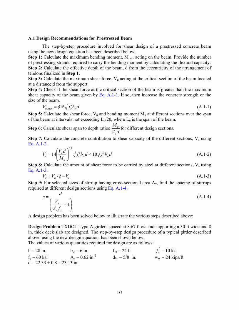
187

A.1 Design Recommendations for Prestressed Beam

The step-by-step procedure involved for shear design of a prestressed concrete beam using the new design equation has been described below: Step 1: Calculate the maximum bending moment, Mmax acting on the beam. Provide the number of prestressing strands required to carry the bending moment by calculating the flexural capacity. Step 2: Calculate the effective depth of the beam, d from the eccentricity of the arrangement of tendons finalized in Step 1. Step 3: Calculate the maximum shear force, Vu acting at the critical section of the beam located at a distance d from the support. Step 4: Check if the shear force at the critical section of the beam is greater than the maximum shear capacity of the beam given by Eq. A.1-1. If so, then increase the concrete strength or the size of the beam.

dbfV wcu ′= 16max, φ (A.1-1) Step 5: Calculate the shear force, Vu and bending moment Mu at different sections over the span of the beam at intervals not exceeding Ln/20, where Ln is the span of the beam.

Step 6: Calculate shear span to depth ratios dV

M

u

u for different design sections.

Step 7: Calculate the concrete contribution to shear capacity of the different sections, Vc using Eq. A.1-2.

dbfM

dVV wcu

uc ′

=

7.0

14 < dbf wc′10 (A.1-2)

Step 8: Calculate the amount of shear force to be carried by steel at different sections, Vs using Eq. A.1-3. cus VVV −= φ/ (A.1-3) Step 9: For selected sizes of stirrup having cross-sectional area Av, find the spacing of stirrups required at different design sections using Eq. A.1-4.

+

=

1yv

s

fAV

ds (A.1-4)

A design problem has been solved below to illustrate the various steps described above: Design Problem TXDOT Type-A girders spaced at 8.67 ft c/c and supporting a 30 ft wide and 8 in. thick deck slab are designed. The step-by-step design procedure of a typical girder described above, using the new design equation, has been shown below. The values of various quantities required for design are as follows:

h = 28 in. bw = 6 in. Ln = 24 ft ′cf = 10 ksi

fy = 60 ksi Av = 0.62 in.2 dbv = 5/8 in. wu = 24 kips/ft d = 22.33 + 0.8 = 23.13 in.

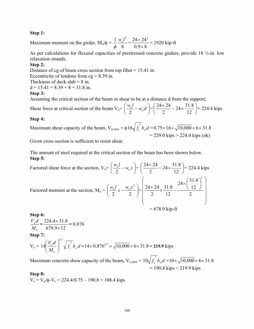
188

Step 1:


1 2lwu

φ=

89.02424 2

×× = 1920 kip-ft

As per calculations for flexural capacities of prestressed concrete girders, provide 18 ½-in. low relaxation strands. Step 2: Distance of cg of beam cross section from top fiber = 15.41 in. Eccentricity of tendons from cg = 8.39 in. Thickness of deck slab = 8 in. d = 15.41 + 8.39 + 8 = 31.8 in. Step 3: Assuming the critical section of the beam in shear to be at a distance d from the support,


− dwlw

uu

2=

×−

×12

8.31242

2424 = 224.4 kips

Step 4:


= 229.0 kips > 224.4 kips (ok) Given cross section is sufficient to resist shear. The amount of steel required at the critical section of the beam has been shown below. Step 5:

Factored shear force at the section, Vu=

− xwlw

uu

2=

×−

×12

8.31242

2424 = 224.4 kips


−

22

2xwxlw uu =

×

−××

212

8.3124

128.31

22424

2

= 678.9 kip-ft Step 6:

u

u

MdV

=129.678

8.314.224×× = 0.876

Step 7:

Vc = dbfM

dVwc

u

u ′

7.0

14 = 8.316000,10876.014 7.0 ×××× = 219.9 kips


= 190.8 kips < 219.9 kips Step 8: Vs = Vu/φ-Vc = 224.4/0.75 – 190.8 = 108.4 kips

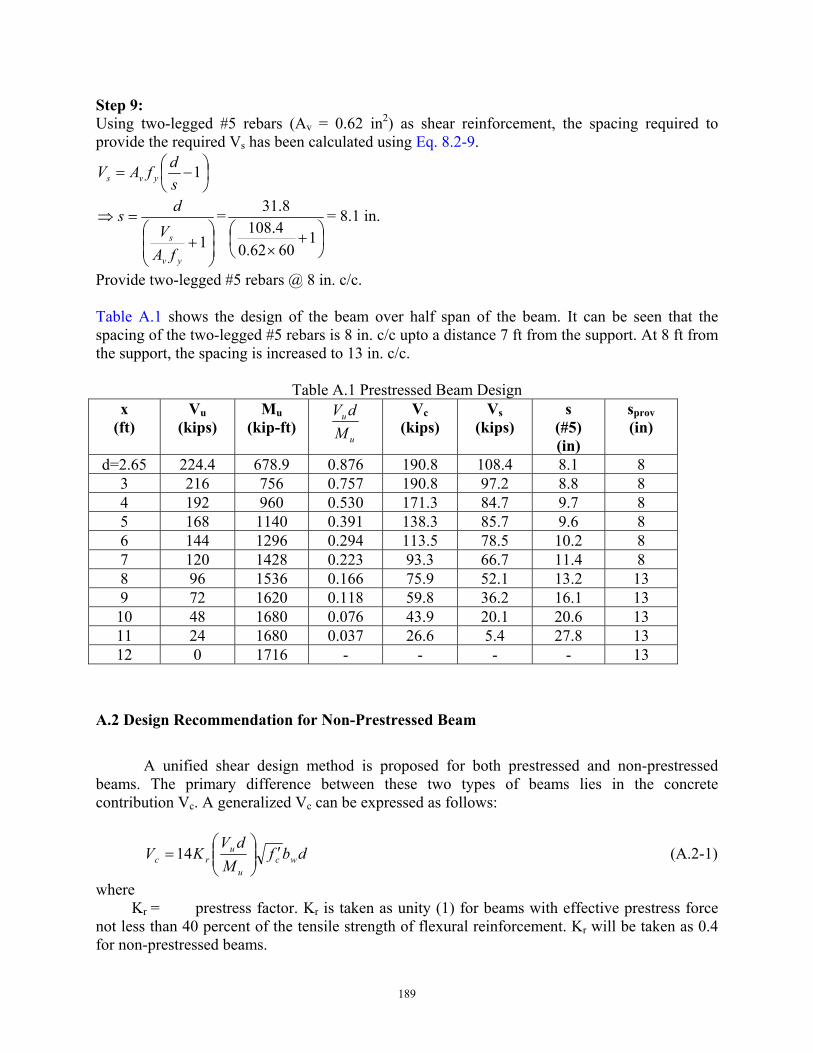
189

Step 9: Using two-legged #5 rebars (Av = 0.62 in2) as shear reinforcement, the spacing required to provide the required Vs has been calculated using Eq. 8.2-9.

−= 1

sdfAV yvs

+

=⇒

1yv

s

fAV

ds =

+

×1

6062.04.1088.31 = 8.1 in.

Provide two-legged #5 rebars @ 8 in. c/c. Table A.1 shows the design of the beam over half span of the beam. It can be seen that the spacing of the two-legged #5 rebars is 8 in. c/c upto a distance 7 ft from the support. At 8 ft from the support, the spacing is increased to 13 in. c/c.

Table A.1 Prestressed Beam Design x

(ft) Vu

(kips) Mu

(kip-ft) u

u

MdV

Vc

(kips) Vs

(kips) s

(#5) (in)

sprov (in)

d=2.65 224.4 678.9 0.876 190.8 108.4 8.1 8 3 216 756 0.757 190.8 97.2 8.8 8 4 192 960 0.530 171.3 84.7 9.7 8 5 168 1140 0.391 138.3 85.7 9.6 8 6 144 1296 0.294 113.5 78.5 10.2 8 7 120 1428 0.223 93.3 66.7 11.4 8 8 96 1536 0.166 75.9 52.1 13.2 13 9 72 1620 0.118 59.8 36.2 16.1 13 10 48 1680 0.076 43.9 20.1 20.6 13 11 24 1680 0.037 26.6 5.4 27.8 13 12 0 1716 - - - - 13

A.2 Design Recommendation for Non-Prestressed Beam

A unified shear design method is proposed for both prestressed and non-prestressed

beams. The primary difference between these two types of beams lies in the concrete contribution Vc. A generalized Vc can be expressed as follows:

dbfM

dVKV wc

u

urc ′

=14 (A.2-1)

where Kr = prestress factor. Kr is taken as unity (1) for beams with effective prestress force

not less than 40 percent of the tensile strength of flexural reinforcement. Kr will be taken as 0.4 for non-prestressed beams.

190

The step-by-step procedure to design a non-prestressed beam using the new design equation has been described below: Step 1: Calculate the maximum bending moment Mmax acting on the beam. Calculate the amount of longitudinal tension steel required to carry this moment. Step 2: Calculate the maximum shear force, Vu acting at the critical section of the beam located at a distance d from the support. Step 3: Check if the shear force at the critical section of the beam is greater than the maximum shear capacity of the beam given by Eq. A.1-1. If so then increase the concrete strength or the size of the beam.

dbfV wcu ′= 10max, φ (A.2-2) Step 4: Calculate the shear force Vu and bending moment Mu at different sections over the span of the beam at intervals not exceeding Ln/20, where Ln is the span of the beam.

Step 5: Calculate shear span to depth ratios u

u

MdV for different design sections.

Step 6: Calculate the concrete contribution to shear capacity of the different sections Vc using Eq. A.2-3.

dbfdbfM

dVKV wcwcu

urc ′<′

= 414

7.0

(A.2-3)

Step 7: Calculate the amount of shear force to be carried by steel at different sections Vs using Eq. A.2-4.

cus VVV −= φ/ (A.2-4) Step 8: For selected sizes of stirrup having cross-sectional area Av find the spacing of stirrups required at different design sections using Eq. A.2-5.

+

=

1yv

s

fAV

ds (A.2-5)

Design Problem An isolated T-beam has an effective span of 25 ft and carries a factored load of 18 kips/ft. Other properties of the beam are as follows: h = 30 in. bf = 40 in. hf = 5 in. bw = 15 in. d = 26 in. cf ′= 7 ksi fy = 60 ksi

Step 1:


1 2lwu

φ=

82518

9.01 2× = 1562.5 kip-ft

Using the compressive stress-strain relations given in the ACI Code (2005) and assuming the NA lies in the flange:

uc Madbaf =

−′

285.0 ,

191

where a = depth over which the compressive stresses exist in the cross section.

Substituting the numerical values of all other parameter in the above equation, the value of a can be obtained: a = 3.23 in. Equating the compressive and steel forces we get:

6023.340785.0

85.0

85.0

×××=⇒

′=⇒

′=

s

y

cs

cys

A

fbafA

baffA

Therefore As = 12.8 in.2 Provide ten #10 bars as longitudinal tension steel (total area = 12.70 in.2 ~ 12.8 in.2) Step 2: Assuming the critical section of the beam in shear to be at a distance d from the support,


− dwlw

uu

2=

×−

×122618

22518 = 186 kips

Step 3:

Maximum shear capacity of the beam, Vu,max = φ dbf wc′10 = 2615000,71075.0 ××××

= 244.7 kips > 186 kips (ok) Given cross section is sufficient to resist shear. Step 4: The amount of steel required at the critical section of the beam has been shown below.


− xwlw

uu

2=

×−

×122618

22518 = 186 kips


−

22

2xwxlw uu =

×

−××

2122618

1226

22518

2

= 445.3 kip-ft Step 5:

u

u

MdV

=123.445

26186×× = 0.905

Step 6:

Vc = dbfM

dVK wcu

ur

′

7.0

14 = 2615000,7905.04.014 7.0 ××××× = 170.4 kips


= 130.5 kips < 170.4 kips

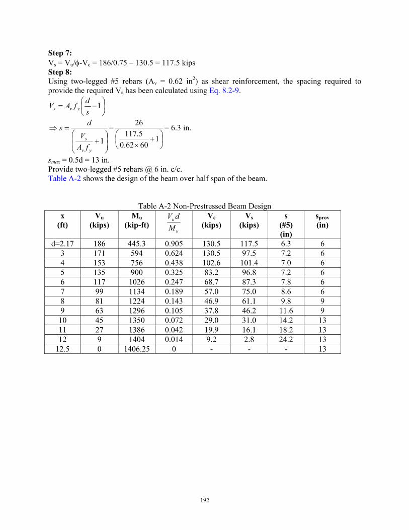
192

Step 7: Vs = Vu/φ-Vc = 186/0.75 – 130.5 = 117.5 kips Step 8: Using two-legged #5 rebars (Av = 0.62 in2) as shear reinforcement, the spacing required to provide the required Vs has been calculated using Eq. 8.2-9.

−= 1

sdfAV yvs

+

=⇒

1yv

s

fAV

ds =

+

×1

6062.05.117

26 = 6.3 in.

smax = 0.5d = 13 in. Provide two-legged #5 rebars @ 6 in. c/c. Table A-2 shows the design of the beam over half span of the beam.

Table A-2 Non-Prestressed Beam Design x

(ft) Vu

(kips) Mu

(kip-ft) u

u

MdV

Vc

(kips) Vs

(kips) s

(#5) (in)

sprov (in)

d=2.17 186 445.3 0.905 130.5 117.5 6.3 6 3 171 594 0.624 130.5 97.5 7.2 6 4 153 756 0.438 102.6 101.4 7.0 6 5 135 900 0.325 83.2 96.8 7.2 6 6 117 1026 0.247 68.7 87.3 7.8 6 7 99 1134 0.189 57.0 75.0 8.6 6 8 81 1224 0.143 46.9 61.1 9.8 9 9 63 1296 0.105 37.8 46.2 11.6 9 10 45 1350 0.072 29.0 31.0 14.2 13 11 27 1386 0.042 19.9 16.1 18.2 13 12 9 1404 0.014 9.2 2.8 24.2 13

12.5 0 1406.25 0 - - - 13

Documents

Technical Report Documentation Page 1. Report … http:// 16. Abstract Prestressed concrete I-beams are used extensively as the primary superstructure components in Texas highway bridges