TECHNICAL REPORT 0-6838-2

TXDOT PROJECT NUMBER 0-6838

BRINGING SMART TRANSPORT TO TEXANS: ENSURING THE BENEFITS OF A CONNECTED AND

AUTONOMOUS TRANSPORT SYSTEM IN TEXAS—FINAL REPORT

Dr. Kara Kockelman (Research Supervisor) with Dr. Stephen Boyles, Paul Avery, Dr. Christian Claudel, Lisa Loftus-Otway, Dr. Daniel Fagnant, Prateek Bansal, Michael W. Levin, Dr. Yong Zhao, Dr. Jun Liu, Lewis Clements, Wendy Wagner, Dr. Duncan Stewart, Dr. Guni Sharon, Dr. Michael Albert, Dr. Peter Stone, Josiah Hanna, Rahul Patel, Hagen Fritz, Tejas Choudhary, Tianxin Li, Aqshems Nichols, Kapil Sharma, and Michele Simoni

CENTER FOR TRANSPORTATION RESEARCH BUREAU OF ENGINEERING RESEARCH THE UNIVERSITY OF TEXAS AT AUSTIN http://library.ctr.utexas.edu/ctr-publications/0-6838-2.pdf

1. Report No.

FHWA/TX-16/0-6838-2

2. Government Accession No.

3. Recipient’s Catalog No.

4. Title and Subtitle

Bringing Smart Transport to Texans: Ensuring the Benefits of a Connected and Autonomous Transport System in Texas – Final Report

5. Report Date

August 2016; Published November 2016

6. Performing Organization Code

7. Author(s)

Dr. Kara Kockelman, Dr. Stephen Boyles, Paul Avery, Dr. Christian Claudel, Lisa Loftus-Otway, Dr. Daniel Fagnant, Prateek Bansal, Michael W. Levin, Dr. Yong Zhao, Dr. Jun Liu, Lewis Clements, Wendy Wagner, Dr. Duncan Stewart, Dr. Guni Sharon, Dr. Michael Albert, Dr. Peter Stone, Josiah Hanna, Rahul Patel, Hagen Fritz, Tejas Choudhary, Tianxin Li, Aqshems Nichols, Kapil Sharma, and Michele Simoni

8. Performing Organization Report No.

0-6838-2

9. Performing Organization Name and Address

Center for Transportation Research The University of Texas at Austin 1616 Guadalupe Street, Suite 4.202 Austin, TX 78701

10. Work Unit No. (TRAIS) 11. Contract or Grant No.

0-6838

12. Sponsoring Agency Name and Address

Texas Department of Transportation Research and Technology Implementation Office P.O. Box 5080 Austin, TX 78763-5080

13. Type of Report and Period Covered

Technical Report

January 2015 – June 2016

14. Sponsoring Agency Code

15. Supplementary Notes Project performed in cooperation with the Texas Department of Transportation and the Federal Highway Administration.

16. Abstract This project develops and demonstrates a variety of smart-transport technologies, policies, and practices for

highways and freeways using connected autonomous vehicles (CAVs), smartphones, roadside equipment, and related technologies. The intent is to maximize the benefit of these technologies in terms of improved driver safety, reduced congestion, and agency cost savings. For example, in a well-implemented system, advanced CAV technologies may reduce current crash costs by at least $390 billion per year. A poorly implemented system could significantly detract from or reverse these benefits.

The project’s Phase 1, documented in this report, showcased DSRC-instrumented vehicles for wrong-way driving alerts, vehicle guidance, and road-surface condition monitoring demonstrations. It developed algorithms for more accurate vehicle-position information and real-time traffic flow monitoring. It delivered statewide and national forecasts of fleet evolution, consumer preferences, and Texans’ opinions of CAV policies and technologies. It also simulated various strategies for smart ramp merges and smart intersection and network operations, under thousands of case settings, with calculated delay reductions. It anticipated emissions savings from more thoughtful automated driving and crash savings from more conflict-aware driving. It also analyzed the benefits of shared autonomous vehicle transit. Recommendations are provided for guiding TxDOT as technologies increasingly become available to the public, estimated to impact the U. S. economy by as much as $1.3 trillion per year. Recommendations focus on the need for increasing TxDOT in-house expertise, simulating new systems, developing policy, and updating design manuals. 17. Key Words

self-driving vehicles, connected vehicles, connected autonomous vehicles, automated vehicles, smart intersections, transport planning, transport law

18. Distribution Statement

No restrictions. This document is available to the public through the National Technical Information Services, Springfield, Virginia 22161; www.ntis.gov.

19. Security Classif. (of report) Unclassified

20. Security Classif. (of this page) Unclassified

21. No. of pages 632

22. Price

Form DOT F 1700.7 (8-72) Reproduction of completed page authorized

Bringing Smart Transport to Texans: Ensuring the Benefits of a Connected and Autonomous Transport System in Texas—Final Report Dr. Kara Kockelman (Research Supervisor) with Dr. Stephen Boyles, Paul Avery, Dr. Christian Claudel, Lisa Loftus-Otway, Dr. Daniel Fagnant, Prateek Bansal, Michael W. Levin, Dr. Yong Zhao, Dr. Jun Liu, Lewis Clements, Wendy Wagner, Dr. Duncan Stewart, Dr. Guni Sharon, Dr. Michael Albert, Dr. Peter Stone, Josiah Hanna, Rahul Patel, Hagen Fritz, Tejas Choudhary, Tianxin Li, Aqshems Nichols, Kapil Sharma, and Michele Simoni

CTR Technical Report: 0-6838-2 Report Date: August 2016 Project: 0-6838 Project Title: Bringing Smart Transport to Texans: Ensuring the Benefit of a Connected

and Autonomous Transport System in Texas Sponsoring Agency: Texas Department of Transportation Performing Agency: Center for Transportation Research at The University of Texas at Austin Project performed in cooperation with the Texas Department of Transportation and the Federal Highway Administration.

Center for Transportation Research The University of Texas at Austin 1616 Guadalupe, Suite 4.202 Austin, TX 78701 http://ctr.utexas.edu/

iv

Disclaimers Author’s Disclaimer: The contents of this report reflect the views of the authors, who are

responsible for the facts and the accuracy of the data presented herein. The contents do not necessarily reflect the official view or policies of the Federal Highway Administration or the Texas Department of Transportation (TxDOT). This report does not constitute a standard, specification, or regulation.

Patent Disclaimer: There was no invention or discovery conceived or first actually reduced to practice in the course of or under this contract, including any art, method, process, machine manufacture, design or composition of matter, or any new useful improvement thereof, or any variety of plant, which is or may be patentable under the patent laws of the United States of America or any foreign country.

Engineering Disclaimer NOT INTENDED FOR CONSTRUCTION, BIDDING, OR PERMIT PURPOSES.

Project Engineer: Kara Kockelman

Professional Engineer License State and Number: Texas No. 93443 P. E. Designation: Research Supervisor

v

Acknowledgments The authors express appreciation to Project Manager Darrin Jensen, and TxDOT

employees Jianming Ma, Travis Scruggs, Melisa Montemayor, Danny Magee, Janie Temple, Joseph Carrizales, Jack Foster, Alex Power, Dale Picha, and Becky Blewett, who served as members of the Project Monitoring Committee. Amy Banker provided most of the administrative support needed to carry out this project, and Maureen Kelly provided extensive editing support. Other project researchers were also instrumental on various facets of the work. These include Tejas Choudhary, Rebecca Hutchinson, Evan Falon, Vincent Recca, Travis Renna, Emilio Longoria, Michael Nelson, Brian Miller, Zack Lofton, Brianna Garner, Gleb Domnenko, Bumsik Kim, Elham Pourrahmani, Amin Mohamadi, Dr. Jia Li, Pavle Bujonav, Dr. Paula Julian, Myra Spector, and Kenneth Perrine.

Related TxDOT Projects This report benefits from work conducted in TxDOT Projects 0-6847 and 0-6849, which

go deeply into the traffic and safety impacts of connected- and automated-vehicles. For details and associated project publications for those and other TxDOT research initiatives, please see the CTR-hosted TxDOT library catalog at http://ctr.utexas.edu/library/.

vi

Table of Contents

Chapter 1. Introduction and Report Summary ..........................................................................1 1.1 Purpose ...................................................................................................................................1 1.2 Organization of Report ..........................................................................................................1 1.3 Evaluating Policies for the Evolving Field of Autonomous Vehicles (Chapter 2) ................1 1.4 Assessing Public Opinions regarding Technologies (Chapter 3) ..........................................3 1.5 Simulation of Network Dynamics (Chapters 4 through 7) ....................................................6

1.5.1 Improvement and Implementation of Dynamic Microtolling (Chapter 5) .....................7 1.5.2 Estimating the Safety Benefits of CAV Technologies (Chapter 6) ................................7 1.5.3 MOVES Emissions Modeling (Chapter 7) .....................................................................8

1.6 Anticipating the Regional Impacts of Connected and Automated Vehicle Travel (Chapter 8) .............................................................................................................................8

1.7 Emerging Transportation Applications (Chapter 9) ..............................................................9 1.8 Technology Demonstrations (Chapters 10 and 11) .............................................................11 1.9 Economic Impacts of CAVs (Chapter 12) ...........................................................................12 1.10 ConOps (Chapter 13) .........................................................................................................13 1.11 Conclusions and Recommendations (Chapter 14) .............................................................13

Chapter 2. Policies for the Evolving Field of Autonomous Vehicles .......................................15 2.1 Background ..........................................................................................................................15

2.1.1 Factual Assumptions that Serve as the Backdrop for the Legal Analysis ....................16 2.2 Legal Developments outside of Texas .................................................................................17

2.2.1 Federal Developments ..................................................................................................18 2.2.2 Other Federal Activities ................................................................................................23 2.2.3 Reports from Federal Agencies.....................................................................................24 2.2.4 Recent Legal Literature .................................................................................................26 2.2.5 State Developments ......................................................................................................28 2.2.6 Overview of State Laws Governing C/AVs ..................................................................32 2.2.7 International Developments ..........................................................................................36 2.2.8 EU Initiatives ................................................................................................................36 2.2.9 Industry Association Activity .......................................................................................41

2.3 The Legality of C/AVs in Texas: Licensing and Related Issues .........................................42 2.3.1 Operation of Motor Vehicles in Texas ..........................................................................42 2.3.2 Rules of the Road and Related Requirements on C/AVs .............................................46

2.4 Tort Liability ........................................................................................................................47 2.4.1 Background on Liability Rules .....................................................................................48 2.4.2 More Complicated Crash Litigation .............................................................................48 2.4.3 New Issues Affecting Governmental Liability .............................................................53 2.4.4 Implications of Liability Challenges for Insurance.......................................................55

2.5 Privacy and Security ............................................................................................................55 2.5.1 Privacy Concerns ..........................................................................................................56 2.5.2 The Law Addressing Privacy Concerns Involving C/AVs ...........................................59 2.5.3 Security Concerns and the Existing Law ......................................................................62

2.6 Conclusions and Recommendations ....................................................................................63 2.6.1 The Need for Immediate and Long-term Planning .......................................................63 2.6.2 Getting from Here to There ...........................................................................................64

vii

2.6.3 Ensuring the Safety of C/AV Testing and Deployment on Public Highways ..............66 2.6.4 Specific Recommendations for TxDOT Headquarters and Divisions ..........................77

Chapter 3. Assessing Public Opinions Regarding Technologies .............................................81 3.1 Introduction ..........................................................................................................................81 3.2 Literature Review ................................................................................................................84

3.2.1 Public Opinion Surveys about Adoption of CAVs .......................................................84 3.2.2 Anticipating Long-Term Adoption of New Technologies ............................................87

3.3 Methodology ........................................................................................................................88 3.3.1 Identifying Professionals ..............................................................................................88 3.3.2 Entities Involved ...........................................................................................................88 3.3.3 Think Group Austin Consultation .................................................................................89 3.3.4 Schedule ........................................................................................................................90

3.4 Discussion Guide Topics .....................................................................................................90 3.5 Key Perceptions ...................................................................................................................91

3.5.1 Planning ........................................................................................................................91 3.5.2 Positives and Negatives ................................................................................................92 3.5.3 Quality of Life ...............................................................................................................92 3.5.4 Environment ..................................................................................................................93 3.5.5 Technology ...................................................................................................................93 3.5.6 Authority, Liability, and Privacy ..................................................................................94 3.5.7 Freight and Transit ........................................................................................................94 3.5.8 Urban Sprawl ................................................................................................................95 3.5.9 Affordability .................................................................................................................95

3.6 Insights and Recommendations ...........................................................................................96 3.6.1 Useful Insights ..............................................................................................................96 3.6.2 Research Opportunities .................................................................................................96 3.6.3 Recommendations .........................................................................................................96

3.7 Survey Design and Data Processing ....................................................................................97 3.7.1 Questionnaire Design and Data Acquisition .................................................................97 3.7.2 Data Cleaning and Sample Correction ..........................................................................97 3.7.3 Geocoding .....................................................................................................................98

3.8 Summary Statistics ..............................................................................................................99 3.8.1 Level 1 and Level 2 Technologies ................................................................................99 3.8.2 Connectivity and Advanced Automation Technologies .............................................102 3.8.3 Opinions about CAV Technologies and Related Aspects ..........................................104 3.8.4 Opinions about AV Usage by Trip Types and Long-distance Travel.........................105

3.9 Forecasting Long-Term Adoption of CAV Technologies .................................................106 3.9.1 Simulation-based Framework .....................................................................................106 3.9.2 Vehicle Transaction and Technology Adoption: Model Specifications .....................108 3.9.3 Forecasted Adoption Rates of CAV Technologies under WTP, Pricing, and

Regulation Scenarios .................................................................................................113 3.10 Assessing Texans’ Opinions about and WTP for Automation and Connected

Vehicle Technologies ........................................................................................................123 3.10.1 Survey Design and Data Processing .........................................................................123 3.10.2 Texans’ Technology-awareness and Safety-related Opinions ..................................125 3.10.3 Key Response Variables ...........................................................................................127

viii

3.10.4 Opinions about AVs ..................................................................................................129 3.10.5 Opinions about CVs ..................................................................................................132 3.10.6 Opinions about Carsharing and Transportation Network Companies ......................133

3.11 Model Estimation .............................................................................................................134 3.11.1 Interest in and WTP to add Connectivity ..................................................................136 3.11.2 WTP for Automation Technologies ..........................................................................137 3.11.3 Adoption Timing of Autonomous Vehicles ..............................................................139 3.11.4 SAV Adoptions Rates under Different Pricing Scenarios ........................................140 3.11.5 Home Location Shifts due to AVs and SAVs ...........................................................145 3.11.6 Support for Tolling Policies ......................................................................................146

3.12 Conclusions ......................................................................................................................149

Chapter 4. Simulation of Network Dynamics..........................................................................152 4.1 Introduction ........................................................................................................................152 4.2 Test Networks Used for Link-Based Meso-simulation .....................................................152

4.2.1 Arterial Networks ........................................................................................................152 4.2.2 Freeway Networks ......................................................................................................153 4.2.3 City Networks .............................................................................................................154

4.3 Effects of Autonomous Vehicles on Networks ..................................................................154 4.3.1 Effects of Autonomous Vehicles on Arterial Networks .............................................155 4.3.2 Effects of Autonomous Vehicles on Freeway Networks ............................................157 4.3.3 Effects of Autonomous Vehicles on City Networks ...................................................160

4.4 Microsimulation using Autonomous Intersection Management (AIM) ............................162 4.5 Summary of Work .............................................................................................................163

Chapter 5. Improvement and Implementation of Dynamic Microtolling ............................165 5.1 Motivation and Problem Definition ...................................................................................165

5.1.1 Computing User Equilibrium ......................................................................................165 5.1.2 Computing System Optimum .....................................................................................165 5.1.3 Approximating Marginal Cost Tolls ...........................................................................166

5.2 Simulation ..........................................................................................................................166 5.2.1 Autonomous Intersection Manager Simulator ............................................................166

5.3 Enhancements to the AIM Simulator .................................................................................167 5.3.1 Macroscopic Model ....................................................................................................167 5.3.2 Example Road-Network ..............................................................................................167 5.3.3 Empirical Evaluation: Macroscopic Model ................................................................168 5.3.4 Computing the Optimal Tolls .....................................................................................169 5.3.5 Evaluating Optimal Tolls using a Macro-Model ........................................................170

5.4 Delta-tolling Technique ( -tolling) ...................................................................................170 5.4.1 Empirical Evaluation of Delta-Tolling .......................................................................172 5.4.2 Representative Road Network ....................................................................................173 5.4.3 Evaluating Optimal Tolls using a Macro-Model ........................................................174

5.5 Conclusions ........................................................................................................................175

Chapter 6. Estimating the Safety Benefits of CAV Technologies ..........................................176 6.1 Typology of Pre-Crash Situations ......................................................................................176 6.2 Monetary and Non-Monetary Measure of the Pre-Crash Scenario Loss ...........................177 6.3 Mapping the Advanced Safety Applications to the Specific Pre-Crash Scenarios ............179

ix

6.4 Effectiveness Assumptions of Safety Applications ...........................................................183 6.5 Crash Savings Results ........................................................................................................190

6.5.1 Conclusions from GES Pre-Crash Scenario Estimates ...............................................193 6.6 Crash Estimates using Safety Surrogate Assessment Model (SSAM) ..............................194

6.6.1 Introduction and Definitions .......................................................................................194 6.6.2 Urban Roadway Bottlenecks .......................................................................................196 6.6.3 Four-way Intersections ................................................................................................199 6.6.4 On Freeway On-Ramps and Off-Ramps .....................................................................201

Chapter 7. MOVES Emissions Modeling ................................................................................211 7.1 Introduction ........................................................................................................................211 7.2 Envisioning Eco-Self-Driving Cycles of Autonomous Vehicles ......................................213

7.2.1 Smoothing Method ......................................................................................................213 7.3 Envisioned CAV Driving Profiles using EPA Cycles .......................................................216 7.4 Envisioned CAV Driving Profiles using Austin Cycles ....................................................219 7.5 Preparing Data Inputs for MOVES ....................................................................................219

7.5.1 Configuring MOVES for Emission Estimations .........................................................219 7.5.2 Data Inputs for MOVES .............................................................................................221

7.6 CAV Emissions Impacts ....................................................................................................222 7.6.1 Emission Estimates using EPA Cycles .......................................................................222 7.6.2 Emissions Estimates using Austin-area Cycles ..........................................................225

7.7 Conclusions ........................................................................................................................229

Chapter 8. Anticipating the Regional Impacts of Connected and Automated Vehicle Travel ..........................................................................................................................................230

8.1 Introduction ........................................................................................................................230 8.2 Literature Review ..............................................................................................................231 8.3 Case Study .........................................................................................................................232

8.3.1 TAZs and Network .....................................................................................................232 8.3.2 Trip Generation ...........................................................................................................234 8.3.3 Trip Distribution .........................................................................................................235 8.3.4 Mode Choice Model ...................................................................................................235 8.3.5 Time-of-Day Model ....................................................................................................236 8.3.6 Traffic Assignment .....................................................................................................236 8.3.7 Travel Cost Feedback .................................................................................................236

8.4 Sensitivity Test Results ......................................................................................................236 8.4.1 Model Results .............................................................................................................238

8.5 Conclusions and Future Work ...........................................................................................241

Chapter 9. Emerging Transportation Applications ................................................................243 9.1 Introduction ........................................................................................................................243 9.2 Transportation Objectives and Performance Measures .....................................................243

9.2.1 Safety ..........................................................................................................................243 9.2.2 Mobility .......................................................................................................................244 9.2.3 Connectivity ................................................................................................................245 9.2.4 Sustainability ...............................................................................................................245 9.2.5 Land Use .....................................................................................................................246 9.2.6 Economic Impacts .......................................................................................................246

x

9.2.7 Summary .....................................................................................................................247 9.2.8 Benefit-Cost Analysis Implementation .......................................................................247

9.3 Benefit-Cost Analysis Implementation ..............................................................................248 9.3.1 Dynamic Route Guidance Systems (DRGS) ..............................................................248 9.3.2 Incident Warning Systems ..........................................................................................252 9.3.3 Congestion Pricing ......................................................................................................253 9.3.4 Intelligent Signals .......................................................................................................257 9.3.5 Cooperative Intersection Collision Avoidance (CICAS) ............................................260 9.3.6 Cooperative Ramp Metering (CRM) ..........................................................................263 9.3.7 Smart Priced Parking (SPP) ........................................................................................265 9.3.8 Shared Autonomous Vehicle Transit ..........................................................................269 9.3.9 Transit with Blind Spot Detect (BSD) and Automatic Emergency Breaking

(AEB) .........................................................................................................................272 9.3.10 Automated Truck-Mounted Attenuator (ATMA) .....................................................274

9.4 Conclusion .........................................................................................................................276

Chapter 10. Demonstration of Technology: SWRI .................................................................278 10.1 Introduction ......................................................................................................................278 10.2 Roadside and Vehicle DSRC Hardware and Applications ..............................................280

10.2.1 Roadside Equipment (RSE) ......................................................................................280 10.2.2 Vehicle: Onboard Equipment (OBE) ........................................................................281

10.3 Connected Vehicle Applications .....................................................................................283 10.3.1 Emergency Vehicle Alert (EVA) ..............................................................................283 10.3.2 Electronic Emergency Brake Lights (EEBL)............................................................284 10.3.3 Static Wrong-way Driving Detection .......................................................................284 10.3.4 Newly Developed Applications ................................................................................285 10.3.5 Road Condition Monitoring ......................................................................................286 10.3.6 Dynamic Wrong-way Driving Detection ..................................................................289

10.4 Demonstrations ................................................................................................................292 10.4.1 Winter 2017, J.J. Pickle Research Campus ...............................................................292 10.4.2 Spring 2016, SwRI and San Antonio Roadways ......................................................293 10.4.3 On SwRI’s Test Track: Dynamic WWD Detection and Alert with AV Safe

Stop ............................................................................................................................294 10.4.4 On and Around Loop 410 in San Antonio ................................................................296

Chapter 11. Demonstration of Technology: CTR ...................................................................298 11.1 Introduction ......................................................................................................................298 11.2 Background ......................................................................................................................298 11.3 IMU-based Traffic Flow Monitoring ...............................................................................301

11.3.1 Inertial Measurement Units .......................................................................................301 11.3.2 Fabrication of a Bluetooth IMU Device ...................................................................301 11.3.3 Validation of the Different Components ...................................................................304 11.3.4 Inertial Data Validation .............................................................................................306 11.3.5 GPS Free Auto Calibration of IMU Onboard Vehicles ............................................307 11.3.6 Trajectory Estimation Using Calibrated IMU Measurements ..................................309

11.4 Fast Computational Scheme for Integrating IMU Data into the LWR Traffic Flow Model .................................................................................................................................310

11.5 Analytical Solutions to the Hamilton-Jacobi Partial Differential Equation (PDE) .........311

xi

11.5.1 The LWR PDE ..........................................................................................................311 11.5.2 The Moskovitz Function ...........................................................................................312 11.5.3 The Generalized Lax-Hopf Formula .........................................................................312 11.5.4 Fast Algorithm for Triangular Fundamental Diagram ..............................................312 11.5.5 Derivation of Internal Conditions for Multiple Bottlenecks .....................................313

Chapter 12. Economic Effects of CAVs ...................................................................................315 12.1 Introduction ......................................................................................................................315 12.2 Industries Analyzed .........................................................................................................316

12.2.1 Automotive ...............................................................................................................316 12.2.2 Electronics and Software Technology ......................................................................318 12.2.3 Trucking/Freight Movement .....................................................................................318 12.2.4 Personal Transport ....................................................................................................319 12.2.5 Auto Repair ...............................................................................................................320 12.2.6 Medical .....................................................................................................................321 12.2.7 Insurance ...................................................................................................................321 12.2.8 Legal Profession ........................................................................................................322 12.2.9 Construction and Infrastructure ................................................................................322 12.2.10 Land Development ..................................................................................................323 12.2.11 Digital Media ..........................................................................................................324 12.2.12 Police (Traffic Violations) ......................................................................................324 12.2.13 Oil and Gas .............................................................................................................325

12.3 Economy-Wide Effects ....................................................................................................325 12.4 Conclusions ......................................................................................................................326

Chapter 13. Concept of Operations (ConOps) ........................................................................328 13.1 Overview and Scope of the Project ..................................................................................328

13.1.1 Background ...............................................................................................................328 13.1.2 Purpose of the Concept of Operations ......................................................................328 13.1.3 Intended Audience ....................................................................................................328 13.1.4 Content and Organization of this Document ............................................................329 13.1.5 Referenced Documents .............................................................................................329

13.2 User-Oriented Operational Description ...........................................................................330 13.2.1 CV Applications ........................................................................................................330 13.2.2 Current CAV Technology .........................................................................................331

13.3 System Overview .............................................................................................................333 13.3.1 Scope and Applicable Physical Environment ...........................................................333 13.3.2 System Goals and Objectives ....................................................................................333 13.3.3 System Capabilities ...................................................................................................333 13.3.4 System Architecture: Physical Components and Interfaces .....................................333

13.4 Operational and Support Environment ............................................................................334 13.5 Operational Scenarios ......................................................................................................335

13.5.1 Emergency Vehicle Alert (EVA) ..............................................................................335 13.5.2 Electronic Emergency Brake Lights (EEBL)............................................................336 13.5.3 Static Wrong-way Driving Detection .......................................................................336 13.5.4 Intelligent Message Propagation (IMP) ....................................................................337 13.5.5 Road Condition Monitoring (RCM) .........................................................................338 13.5.6 Dynamic Wrong-way Driving and Road Hazard Detection .....................................339

xii

Chapter 14. Conclusions and Recommendations ....................................................................341 14.1 Specific Recommendations for TxDOT Headquarters and Divisions .............................342

14.1.1 Shaping Legislative Policy on CAVs .......................................................................342 14.1.2 Short-Term Practices.................................................................................................343 14.1.3 Mid-Term Practices ..................................................................................................344 14.1.4 Long-Term Practices .................................................................................................345

References ...................................................................................................................................346 Appendices Table of Contents (provided as separate document)

Appendix A: List of All Possible Attendees ....................................................................................1

Appendix B: Emails to Obtain Focus Group Participants ...............................................................7

Appendix C: Final List of Focus Group Attendees .........................................................................9

Appendix D: Focus Group Discussion Guide ................................................................................11

Appendix E: Topline Report from Focus Group Consultants .......................................................16

Appendix F: Surveys Used for Data Collection on Projects 0-6838, 0-6847, and 0-6849 ............27

Appendix G: Collection of “Guidelines or Model” State Laws (Not Necessarily Enacted) .......141

Appendix H: Analysis of Product Liability Claims against OEMs in Texas in Car Crashes involving C/AVs ....................................................................................................................215

Appendix I. Expert Survey Questionnaire ...................................................................................238

Appendix J. Expert Interview Questions .....................................................................................243

Appendix K. Case Law and Statutes ............................................................................................244

xiii

List of Figures

Figure 2.1: Automated Private Vehicle Pathway .......................................................................... 16 Figure 2.2: Example of Vehicle’s Cybersecurity Mitigation Technologies Shown along

an In-Vehicle Network ...................................................................................................... 25 Figure 2.3: SAE International’s Definitions of Autonomous Vehicle Levels (J3016

Standard) ........................................................................................................................... 42 Figure 2.4: Data Components in V2V Technology ...................................................................... 57 Figure 3.1: Geocoded Respondents across Continental USA ....................................................... 98 Figure 3.2: Interest in Automation Technologies ......................................................................... 99 Figure 3.3: The Simulation-based Framework to Forecast Long-term Technology

Adoption ......................................................................................................................... 108 Figure 3.4: Estimated Shares of US Light-Duty Vehicles with Advanced Automation ............ 121 Figure 3.5: Geocoded Respondents across Texas ....................................................................... 124 Figure 4.1: Lamar and 38th Street and Congress Avenue Networks (from left to right) ........... 153 Figure 4.2: I 35, Hwy 290, and MoPac Networks (from left to right) ........................................ 153 Figure 4.3: Arterial Network Travel Time Results for Lamar & 38th, and Congress Ave. ....... 157 Figure 4.4: Freeway Network Travel Time Results for I-35 ...................................................... 158 Figure 4.5: Freeway Network Travel Time Results for MoPac and US 290 .............................. 160 Figure 4.6: Downtown Austin Network ..................................................................................... 161 Figure 4.7: Interaction between Human Drivers, Driver Agents, and the Intersection

Manager .......................................................................................................................... 164 Figure 4.8: Average Delay vs. Different Ratio of Autonomous/Human Drivers at Traffic

Level of 360 Vehicles/Lane/Hour ................................................................................... 164 Figure 5.1: Example Road Network within the AIM Simulator ................................................. 168 Figure 5.2: A Representative Road Network .............................................................................. 173 Figure 5.3: Average Travel Time, Utility, and SU as a Function of β for the

Representative Road Network ........................................................................................ 174 Figure 6.1: Low-Flow Conflicts Disaggregated by Type ........................................................... 197 Figure 6.2: Medium-Flow Conflicts Disaggregated by Type ..................................................... 197 Figure 6.3: High-Flow Conflicts Disaggregated by Type .......................................................... 198 Figure 6.4: Four-way Conflicts Disaggregated by Type ............................................................ 200 Figure 6.5: On-Off Ramp Conflicts Disaggregated by Type ...................................................... 201 Figure 6.6: Intersection of I-35 and Wells Branch Parkway Conflicts Disaggregated by

Type ................................................................................................................................ 202 Figure 6.7: Number of Conflict Types Aggregated by Simulation Type ................................... 205 Figure 6.8: Conflicts at Intersection of Manor Road and E M Franklin Avenue ....................... 208 Figure 7.1: An EPA Driving Cycle for Conventional Vehicles on Highway Driving

Conditions ....................................................................................................................... 212

xiv

Figure 7.2: Driving Cycle Example (Smoothed CAV Cycle vs. Original HV Cycle) ............... 215 Figure 7.3: Distributions of Acceleration and Decelerations: Before Smoothing and After

Smoothing at Different Smoothing Factors .................................................................... 216 Figure 7.4: EPA Driving Cycles Before (blue solid line) and After (red dashed line) the

Smoothing ( =0.22999) .................................................................................................. 218 Figure 7.5: Emission Estimates for VOC ................................................................................... 222 Figure 7.6: Emission Estimates for PM2.5, CO, NOx, and CO2 ............................................... 224 Figure 7.7: Distributions of Emissions Reductions (in percentages) of VOC, PM2.5, CO,

NOx, SO2, and CO2 ......................................................................................................... 226 Figure 8.1: TAZ System for CAMPO Region ............................................................................ 233 Figure 8.2: CAMPO Model Network ......................................................................................... 234 Figure 8.3: Mode Choice Model Structure ................................................................................. 235 Figure 8.4: Map of Downtown Austin with AM Period Parking Costs...................................... 241 Figure 9.1: Collision Risk Increase for DRGS Cars ................................................................... 250 Figure 9.2: GlidePath Application Overview ............................................................................. 260 Figure 9.3: SFpark Pilot and Control Area ................................................................................. 267 Figure 10.1: SwRI CAV Technologies and Resources ............................................................... 279 Figure 10.2: Example of RSE ..................................................................................................... 281 Figure 10.3: Example of RSE ..................................................................................................... 281 Figure 10.4: San Antonio RSE Installation Locations ................................................................ 281 Figure 10.5: SwRI POD Architecture ......................................................................................... 282 Figure 10.6: SwRI PODS on Test Bench ................................................................................... 282 Figure 10.7: SwRI Pod Internal .................................................................................................. 283 Figure 10.8: EVA ........................................................................................................................ 284 Figure 10.9: SwRI Tablet Display EEBL Message .................................................................... 284 Figure 10.10: Connected Vehicle WWD Messages Sent by RSE .............................................. 285 Figure 10.11: Simulated CVs along I-410 in San Antonio Showing Potential for Message

Propagation between RSEs ............................................................................................. 286 Figure 10.12: RCM Hardware Evolution.................................................................................... 287 Figure 10.13: High-level Overview of the DDRR System. ........................................................ 287 Figure 10.14: The Distribution of Readings from the DDRR System. ....................................... 288 Figure 10.15: Heatmap Display of Road Condition in San Antonio, TX ................................... 289 Figure 10.16: Showing Precise Location of Anomalous Events ................................................ 289 Figure 10.17: Dynamic Lane Learning ....................................................................................... 291 Figure 10.18: Winter Demonstration Venue Showing J.J. Pickle Research Campus

(Inset), and Detail Location of Test Road and Temporary RSE ..................................... 292 Figure 10.19: Winter Demonstration Venue Showing Effective RSE Coverage Area,

Viewing Area, and CV Vehicles During a Demonstration ............................................. 293

xv

Figure 10.20: Spring Demonstration Venue Showing the Campus of SwRI and a Portion of Interstate 410 Instrumented with RSEs ...................................................................... 294

Figure 10.21: Dynamic Lane Learning at SwRI’s Test Track .................................................... 295 Figure 10.22: SwRI’s Autonomous Freightliner Stops Once Identified as a WWD .................. 295 Figure 10.23: SwRI Autonomous Freightliner ........................................................................... 295 Figure 10.24: Road Condition Monitoring Tablet and Heat Map Displays ............................... 296 Figure 10.25: Message Propagation Demonstration Configuration ........................................... 297 Figure 11.1: Illustration of a Constellation of GPS Satellites Orbiting the Earth ....................... 299 Figure 11.2: Architecture of Classical Traffic Monitoring Systems (Probe-Vehicle

Based). ............................................................................................................................ 300 Figure 11.3: Architecture of a Distributed Probe-Based Traffic Flow Monitoring System,

which Guarantees User Privacy. ..................................................................................... 300 Figure 11.4: Top: Early IMU Prototype. Bottom: Second Iteration of the PCB Layout. ........... 302 Figure 11.5: Bluetooth, IMU, and SD Card Peripherals of the Developed Sensor .................... 303 Figure 11.6: GPS and JTAG Programming Interface of the Sensor ........................................... 303 Figure 11.7: JTAG Programming System. Left: RS232 Interface. Right: JLink

Programmer..................................................................................................................... 304 Figure 11.8: IMU Device Installed in a Vehicle, with Power Supplied through a USB Car

Charger ............................................................................................................................ 304 Figure 11.9: Illustration of Inertial Data Reception on a Bluetooth-enabled Smartphone ......... 305 Figure 11.10: Norm of the Acceleration Vector (Units: / 2) ............................................... 306 Figure 11.11: Acceleration (Unit: / 2) along the Three Axes of the Accelerometer

during a Car Trip. ............................................................................................................ 307 Figure 11.12: Rotation Rate Measurement Data (Units: / ) .............................................. 307 Figure 11.13: Convergence of the Attitude Angle Estimates (attitude of the IMU device

with respect to the vehicle) Derived from the Rotation Matrix Rs/c ............................... 309 Figure 11.14: Example of Simulation of Several Moving Bottlenecks. ..................................... 314 Figure 13.1: Applications Defined by the USDOT .................................................................... 331 Figure 13.2: RSE DSRC Roadside Device Manufactured by Coda Wireless ............................ 332 Figure 13.3: RSE DSRC Roadside Device Manufactured by Savari ......................................... 332 Figure 13.4: OBE DSRC Vehicle Devices Manufactured by Cohda Wireless .......................... 332 Figure 13.5: OBE DSRC Vehicle Devices Manufactured by Savari .......................................... 333 Figure 13.6: SET-IT Physical Diagram for EVA ....................................................................... 334 Figure 13.7: EVA Scenario ......................................................................................................... 336 Figure 13.8: Potential In-vehicle Display of EEBL Message ..................................................... 336 Figure 13.9: CV WWD Messages Sent by RSE ......................................................................... 337 Figure 13.10: Simulated CVs along I-410 in San Antonio Showing Potential for Message

Propagation Between RSEs ............................................................................................ 338 Figure 13.11: Incident Data Sent to TxDOT .............................................................................. 339 Figure 13.12: Smart Transport System Lane Learning ............................................................... 340

xvi

List of Tables

Table 2.1: Key Practices to Identify and Mitigate Vehicle Cybersecurity Vulnerabilities Identified by Industry Stakeholders .................................................................................. 25

Table 2.2: Strategy Checklist for Government Promotion of Automated Driving ....................... 27 Table 2.3: Enacted State Legislation Governing Autonomous Vehicles ...................................... 29 Table 2.4: Matrix of Topic Areas for C/AV Policies in Texas ..................................................... 66 Table 3.1: Count of Involved Entity Types .................................................................................. 89 Table 3.2: Additional Attendees ................................................................................................... 90 Table 3.3: Focus Group Meeting Schedule ................................................................................... 90 Table 3.4: Population-weighted Summaries for Level 1 and Level 2 Technologies .................. 101 Table 3.5: Population-weighted WTP for Adding Connectivity and Advanced

Automation Technologies ............................................................................................... 103 Table 3.6: Population-weighted Average WTP for Automation Technologies .......................... 103 Table 3.7: Individual-weighted Opinions of Respondents ......................................................... 104 Table 3.8: Individual-weighted Opinions about Connectivity and AVs’ Production ................. 105 Table 3.9: Individual-weighted Summaries for AV Usage by Trip Type .................................. 105 Table 3.10: Population-weighted Summary Statistics of Explanatory Variables ....................... 109 Table 3.11: Transaction Decisions (Weighted Multinomial Logit Model Results) .................... 111 Table 3.12: Bought Two Vehicles? (Binary Logit Model Results) ............................................ 112 Table 3.13: Bought New Vehicle? (Binary Logit Model Results) ............................................. 113 Table 3.14: WTP Increase, Tech-Pricing Reduction, and Regulation Scenarios ....................... 114 Table 3.15: Technology Prices at 5% Annual Price Reduction Rates ........................................ 115 Table 3.16: Estimated Shares of US Light-Duty Vehicles with CAV-related Technologies

in Scenarios 1 and 2 ........................................................................................................ 117 Table 3.17: Estimated Shares of US Light-Duty Vehicles with CAV-related Technologies

in Scenarios 3 and 4 ........................................................................................................ 118 Table 3.18: Estimated Shares of US Light-Duty Vehicles with CAV-related Technologies

in Scenarios 5 and 6 ........................................................................................................ 119 Table 3.19: Estimated Shares of US Light-Duty Vehicles with CAV-related Technologies

in Scenarios 7 and 8 ........................................................................................................ 120 Table 3.20: Population-weighted Summary Statistics of Explanatory Variables ....................... 126 Table 3.21: Population-weighted Results of WTP for and Opinions about Connectivity

and Automation Technologies ........................................................................................ 128 Table 3.22: Population-weighted Opinions about SAV Adoption Rates, Congestion

Pricing, and Home Location Shifting ............................................................................. 129 Table 3.23: Population-weighted Opinions about Level 4 Self-driving Technology ................. 131 Table 3.24: Major Concerns and Benefits Associated with AVs ............................................... 132 Table 3.25: Current Adoption and Interest in Connectivity Features ......................................... 133

xvii

Table 3.26: Support for CV-related Strategies and Improvements in Automobile Technologies ................................................................................................................... 133

Table 3.27: Opinions about Carsharing and On-demand Taxi Services ..................................... 134 Table 3.28: Interest in Connectivity Model Results (using OP) ................................................. 137 Table 3.29: WTP for Connectivity Model Results (using IR) .................................................... 137 Table 3.30: WTP for Automation Technologies Model Results (using IR) ............................... 139 Table 3.31: Adoption Timing of AVs Model Results (using OP) .............................................. 140 Table 3.32: SAV Adoption Rates under Different Pricing Scenarios Model Results (using

OP) .................................................................................................................................. 142 Table 3.33: Home Location Shifts due to AVs and SAVs Model Results (using OP) ............... 145 Table 3.34: Support for Tolling Policies Model Results (using OP) .......................................... 147 Table 4.1: Downtown Austin City Network Travel Time Results ............................................. 161 Table 4.2: Semi-CAV Technologies ........................................................................................... 163 Table 5.1: Toll Values and Travel Times ................................................................................... 169 Table 5.2: The Different Parameters, Variables, and Properties of ∆-tolling and Macro-

Model Tolling ................................................................................................................. 172 Table 5.3: Average Travel Time, Utility, and SU for β Values 8, 20, 80 ................................... 175 Table 6.1: Mapping of Crash Types to New Pre-Crash Scenario Typology .............................. 177 Table 6.2: KABCO to MAIS Translator ..................................................................................... 178 Table 6.3: Unit Costs of Policed-Reported Crashes, 2013 Dollars ............................................. 179 Table 6.4: Mapping Pre-crash Scenarios to CAV Technologies ................................................ 181 Table 6.5: CRF (Cumulative) Assumptions of the Fatal Crashes in Conservative Scenario ..... 184 Table 6.6: CRF (Cumulative) Assumptions of the Fatal Crashes in Moderate Scenario ........... 186 Table 6.7: CRF (Cumulative) Assumptions of the Fatal Crashes in Aggressive Scenario ......... 188 Table 6.8: Annual Crash Counts of U.S. Light-Duty-Vehicle Pre-Crash Scenarios (using

2013 GES crash records) ................................................................................................ 191 Table 6.9: Economic Costs and Comprehensive Costs of All U.S. Light-Duty-Vehicle

Pre-Crash Scenarios (using 2013 GES crash records) .................................................... 192 Table 6.10: Annual Economic & Comprehensive Cost Savings Estimates for Fully

Automated Light-Duty Vehicle Application under Three Scenarios (using 2013 GES Crash Records) ....................................................................................................... 193

Table 6.11: SSAM Measures and Definitions ............................................................................ 195 Table 6.12: Bottleneck Conflict Results Disaggregated by Type ............................................... 196 Table 6.13: Percent Difference in Conflicts Between HVs and AVs ......................................... 196 Table 6.14: Bottleneck Surrogate Safety Measures (Number of Measures) .............................. 198 Table 6.15: Percent Differences in Safety Measures between HVs and AVs (Bottleneck,

Number of Measures) ..................................................................................................... 199 Table 6.16: Four-way Intersection Conflicts Disaggregated by Type (Number of

Conflicts)......................................................................................................................... 199 Table 6.17: Four-way Intersection Surrogate Safety Measures (Number of Measures) ............ 200

xviii

Table 6.18: Percent Differences in Safety Measures between HVs and AVs (Four-way, Number of Measures) ..................................................................................................... 200

Table 6.19: On-Ramp/Off-Ramp Conflicts Disaggregated by Type (Number of Conflicts) ..... 201 Table 6.20: On-Off Ramp Surrogate Safety Measures (Number of Measures) ......................... 202 Table 6.21: Intersection of I-35 and Wells Branch Parkway Conflict Summary (Number

of Conflicts) .................................................................................................................... 203 Table 6.22: Intersection of I-35 and Wells Branch Parkway Surrogate Safety Measures

(Number of Measures) .................................................................................................... 203 Table 6.23: Intersection of I-35 and Wells Branch Parkway Conflict Summary (Number

of Crashes) ...................................................................................................................... 204 Table 6.24: Intersection of I-35 and Wells Branch Parkway Surrogate Safety Measures

(Number of Measures) .................................................................................................... 204 Table 6.25: Intersection of I-35 and Wells Branch Parkway Conflicts Summary (Number

of Conflicts) .................................................................................................................... 204 Table 6.26: Intersection of I-35 and Wells Branch Parkway Surrogate Safety Measures

(Number of Measures) .................................................................................................... 205 Table 6.27: Intersection of I-35 and 4th Street Conflicts Summary (Number of Conflicts) ...... 206 Table 6.28: Intersection of I-35 and 4th Street Surrogate Safety Measures (Number of

Measures) ........................................................................................................................ 206 Table 6.29: Intersection of I-35 and 4th Street Conflicts Summary (Number of Conflicts) ....... 206 Table 6.30: Intersection of I-35 and 4th Street Surrogate Safety Measures (Number of

Measures) ........................................................................................................................ 207 Table 6.31: Intersection of I-35 and 4th Street Conflict Summary (Number of Conflicts) ......... 207 Table 6.32: Intersection of I-35 and 4th Street Surrogate Safety Measures (Number of

Measures) ........................................................................................................................ 207 Table 6.33: Intersection of Manor Road and E M Franklin Avenue Conflicts Summary

(Number of Conflicts) ..................................................................................................... 208 Table 6.34: Intersection of Manor Road and E M Franklin Avenue Surrogate Safety

Measures (Number of Measures) .................................................................................... 209 Table 6.35: Intersection of Manor Road and E M Franklin Avenue Surrogate Safety

Measures (Number of Conflicts) .................................................................................... 209 Table 6.36: Intersection of Manor Road and E M Franklin Avenue Surrogate Safety

Measures (Number of Measures) .................................................................................... 209 Table 6.37: Intersection of Manor Road and E M Franklin Avenue Surrogate Safety

Measures (Number of Conflicts) .................................................................................... 210 Table 6.38: Intersection of Manor Road and E M Franklin Avenue Surrogate Safety

Measures (Number of Measures) .................................................................................... 210 Table 7.1: EPA Cycles ................................................................................................................ 217 Table 7.2: Summary Statistics of Emissions-Related Variables ................................................. 225 Table 7.3: Regression Results for Y = % Emission Reductions, as a Function of Vehicle,

Fuel Type, Starting Engine Temperature, and Average Speed ....................................... 228

xix

Table 8.1: Destination Choice Model Parameters ...................................................................... 235 Table 8.2: Multinomial Logit Model Parameters in the Scenarios ............................................. 236 Table 8.3: CAMPO Model Time of Day Periods Definition ...................................................... 236 Table 8.4: Scenario Assumptions on Key Parameters (Relative to Base-Case/No-AV

Scenario) ......................................................................................................................... 238 Table 8.5: Regional VMT Forecasts during AM Peak Period .................................................... 239 Table 8.6: Downtown Austin VMT during AM Peak Period ..................................................... 241 Table 9.1: Texas Crash Costs, by Type (in 2015 dollars) ........................................................... 244 Table 9.2: Economic Impact Measures ....................................................................................... 247 Table 9.3: Summary of Transportation Objective Performance Measures ................................. 247 Table 9.4: Potential Delay Reduction Benefits from DRGS ...................................................... 248 Table 9.5: Potential Annual Delay Reduction Benefits from DRGS, as Applied in Austin ....... 249 Table 9.6: Emission Savings Estimates for QuickRide in Texas ................................................ 254 Table 9.7: Summary of Current Emission Levels, Estimated Changes, and Monetization

Values ............................................................................................................................. 255 Table 9.8: Congestion Pricing Capital Costs .............................................................................. 256 Table 9.9: Congestion Pricing Operating Costs. ......................................................................... 257 Table 9.10: Benefit-Cost Ratios of Congestion Pricing Strategies ............................................. 257 Table 9.11: Major Findings on MMITSS ................................................................................... 259 Table 9.12: CICAS Programs ..................................................................................................... 261 Table 9.13: Benefit-Cost Analysis of CICAS, as Applied to One of Austin’s Top 25

Highest Crash Intersections ............................................................................................ 262 Table 9.14: Estimated Costs of CRM ......................................................................................... 264 Table 9.15: Benefit-Cost Analysis of CRM ................................................................................ 265 Table 9.16: Strategies of SFMTA ............................................................................................... 266 Table 9.17: Benefit-Cost Analysis of SPP in Houston ............................................................... 269 Table 9.18: Anticipated SAV Life-Cycle Emissions Outcomes Using the Austin

Network-Based Scenario (Per SAV Introduced) ............................................................ 270 Table 9.19: Cost Parameters for Driverless Vehicles in a Shared Fleet ..................................... 272 Table 9.20: Benefit-Cost Analysis of BSD and AEB ................................................................. 274 Table 9.21: Rear-End Crash Cost in the Highest Risk Work Zones ........................................... 275 Table 9.22: ATMA Benefit-Cost Analysis ................................................................................. 276 Table 10.1: SwRI Standards Participation Related to ATMS/ATIS/CV/AV ............................. 280 Table 12.1: Summary of Annual Economic Effects (Industry and Economy-Wide) ................. 327

xx

List of Acronyms

ATMA automated truck-mounted attenuator

AV autonomous vehicle (fully automated)

BSM basic safety message

CAV connected autonomous vehicle (a communicating and self-driving vehicle)

C/AV connected and/or automated vehicle (not necessarily fully automated)

ConOps concept of operations

CV connected vehicle

CVRIA Connected Vehicle Reference Implementation Architecture

DOT department of transportation

DSRC dedicated short-range communication

FHWA Federal Highway Administration

FTC Federal Trade Commission

GAO Government Accountability Office

IR interval regression

ITS intelligent transportation system

HV human-driven vehicle

MMITS Multi-Modal Intelligent Traffic Signal System

NHTSA National Highway Traffic Safety Administration

OBE onboard equipment

OP ordered probit

POD portable onboard device

RSE roadside equipment

SwRI Southwest Research Institute

TxDOT Texas Department of Transportation

V2I vehicle to infrastructure

V2V vehicle to vehicle

WTP willingness to pay

1

Chapter 1. Introduction and Report Summary

1.1 Purpose

Smart-driving technologies are changing the landscape of transportation. Great mobility, safety, and environmental benefits are anticipated from these technologies, which enable safer and more comfortable driving in general. However, in order to realize the maximum potential benefits for the overall transportation system in Texas, these technologies alone are not enough. Rather, policymaking and innovation in infrastructure and operations strategies, among other measures, are crucial.

This project develops and demonstrates a variety of smart-transport technologies, policies, and practices for Texas highways and freeways using autonomous vehicles (AVs), connected vehicles (CVs), smartphones, roadside equipment, and related technologies.

The work’s products provide ideas and equipment for more efficient intersection, ramp, and weaving section operations for connected autonomous vehicle (CAV) operations, alongside a suite of behavioral and traffic-flow forecasts for Texas regions and networks under a variety of vehicle mixes (smart plus conventional, semi-autonomous versus fully autonomous, connected but not automated). The work provides rigorous benefit-cost assessments of multiple strategies that the Texas Department of Transportation (TxDOT) may pursue to bring smarter, safer, more connected, and more sustainable ground transportation systems to Texas, in concert with auto manufacturers, technologists, and the traveling public. The effort supports proactive policymaking on vehicle- and occupant-licensing, liability, and privacy standards, as technologies become available and travel behaviors change.

The project’s Phase 1 demonstrations showcased dedicated short-range communications (DSRC) technologies on The University of Texas at Austin’s Pickle Research Campus in Austin and then on the Southwest Research Institute (SwRI) campus in San Antonio, for application of driver alerts, road-surface conditions, and traffic flow monitoring, as well as vehicle guidance.

1.2 Organization of Report

The organization of this report largely follows the chronological order of the project work, including a series of distinctive and meaningful tasks, from legal analyses to travel behavior and fleet forecasting, and from traffic simulations with smart and micro-tolled intersections and ramp controls to design and demonstrations of location-finding and CV applications for better traffic management, road condition monitoring, and safety improvements across Texas. The following sub-sections offer executive summaries of each chapter of this extensive report, to provide readers an overview of contents and findings.

1.3 Evaluating Policies for the Evolving Field of Autonomous Vehicles (Chapter 2)

Chapter 2 investigates the legal status and near-term issues associated with the liability, licensing, and privacy of connected and/or automated vehicles (C/AVs) in Texas. Although this reconnaissance work considers the law from numerous vantage points, particular attention was paid to how the introduction of C/AVs may affect the priorities, liability, and responsibilities of TxDOT.

2

Numerous public benefits are associated with C/AVs, but these technologies also present risks and challenges to our transportation systems. Since nearly all of the pertinent laws and legal requirements governing auto-safety and transportation were passed decades before the development of AVs, there is a growing concern that at least some of the safety and privacy risks posed by C/AVs to the public in general and consumers in particular will fall outside the protections afforded by current laws and regulations. Indeed, because existing laws do not address C/AV technologies directly, they could have an unintended effect on the future of C/AVs. Some laws may unwittingly impede the deployment of C/AVs by imposing unnecessary constraints, while other laws may do too little to address new risks arising from potential invasions of privacy, security, and even the management of unique safety hazards posed by C/AVs.

The analysis begins with a review of the law emerging outside of Texas—at the national level, in several states that have developed legislation specifically governing C/AVs, and internationally. The task then considered how the Texas legal system will intersect with this new technology. The analysis reviews existing Texas laws and regulations to determine whether C/AVs are currently “legal” in Texas without added legislation and regulation; whether and how existing liability rules might adapt to accidents involving C/AVs; and how the citizens of the State can ensure that their privacy is protected as C/AVs become prevalent on Texas roadways.

This bird’s-eye-view of the intersection of the law and the use of C/AVs in Texas revealed several areas that deserve legislative and regulatory attention (as well as additional research) in the near term. First and perhaps most immediate is the need for policymakers to consider whether the testing and deployment of C/AVs in the State will benefit from more formal, legal oversight. The existing laws in Texas do not seem to contemplate the emergence of driverless or passively operated cars, and yet, as currently drafted, the deployment of vehicles without drivers (albeit with one “operator” somewhere in the vehicle) appears to be legal. Presumably, then, any person with a valid driver’s license could retrofit and operate a driverless vehicle legally on Texas public roadways, without additional regulatory oversight, restrictions, or other operational requirements.

A second near-term issue at the intersection of C/AVs and Texas law that emerges from the research is the need for some adjustments to current liability rules to provide greater predictability—particularly to TxDOT—as C/AVs are tested and deployed on Texas roadways. Some anticipatory legislative direction could lay essential groundwork: a clarification of what constitutes “notice” of a malfunction in traffic devices in the wake of electronic signals; clarifications of what constitutes road hazards that need to be reasonably addressed with respect to C/AVs; and direction for several other discrete liability-related issues. There is also growing concern that tort litigation over run-of-the-mill car crashes will become considerably more complicated with the use of C/AVs—future crash litigation will likely include costly product liability claims against manufacturers as well as simpler claims against operators for violations of the law. A review of existing tort liability laws and State legislation that anticipates and addresses the complexity of this future C/AV crash litigation will be beneficial. A detailed analysis of product liability claims against OEMS in Texas was also undertaken and can be found in the appendices.

Finally, C/AVs present a number of important public conflicts arising at the intersection of driver privacy, autonomy, and security. The National Highway Traffic Safety Administration (NHTSA) and the Federal Trade Commission appear to be taking primary responsibility in the development of national standards and directives for C/AV designs to heighten consumer privacy and security. Yet, C/AVs also raise State-specific concerns relating to whether and how private data about individual drivers can be accessed. Such concerns include, for example, requirements under the Texas Open Records Act that currently may oblige agencies to disclose certain personal

3

travel-related information on Texas citizens. To anticipate and limit some of the most preventable intrusions into privacy, relatively modest amendments to existing laws are proposed.

Under Texas law, C/AVs appear to be legal on State highways without special notice, insurance, certifications, testing, or reporting. Texas agencies are also likely to face increased liabilities with respect to these vehicles and increased pressure to manage and share personal data on registered owners and/or drivers of these vehicles. State agencies will also find themselves under increased pressure for the special CAV use of roadways—such as truck platoons, and driverless and empty (zombie) cars. Without legislation addressing these issues, State agencies and some local governments may find themselves not only without legislative guidance, but in some cases, blocked or constrained by existing laws, in their ability to resolve conflicts in ways that appear consistent with the larger public interest. Chapter 2 concludes by charting out a number of additional legislative initiatives that should facilitate a smooth integration of C/AVs onto Texas highways, both by providing predictability to the C/AV industry and increasing the public’s trust in the safety of the vehicles.

1.4 Assessing Public Opinions regarding Technologies (Chapter 3)

Since the motoring public is a key force in how the vehicle automation future will unfold, understanding their current opinions about and plans for CAV technology adoption is important. This chapter documents various insights related to planning for CAVs; change in quality of life given vehicle automation; emission-based impacts of CAVs; professionals’ perceptions of authority, liability, and privacy issues in new vehicle technologies; impact of automation on freight and transit; and change in urban sprawl.

To obtain information on stakeholder understanding and interests, the project team conducted four focus groups, and designed and disseminated two extensive surveys. Two of the focus groups took place in Austin and two took place in San Antonio. The 35 planning professionals who served as participants in these four focus groups tend to agree that implementation decisions regarding CAVs—such as security, regulations, manufacturing, and testing—must come from the state or federal level. Local jurisdictions will lack the funding or delegated power, and implementation may vary among localities, and across land-use types (e.g., suburban versus rural settings). Additionally, an information campaign could be very helpful in disseminating knowledge among those who will make important local changes, including policymakers and planners.

In the first of the two online surveys, 2,167 Americans (including 1,364 Texans) provided complete responses that were used in a detailed personal-vehicle fleet-evolution model, designed to simulate Americans’ long-term (2015 to 2045) adoption of CAV technologies. These simulations included eight scenarios based on evolving technology prices (using 5% and 10% annual reduction rates, thanks to technological advances and economies of scale in production over time), changing willingness to pay (WTP) (growing at 0%, 5%, and 10% annual increments over time, to reflect society’s greater familiarity with such technologies and their benefits over time), and different regulations (as related to electronic stability control [ESC] and DSRC-based connectivity requirements on all new vehicles sold). The survey investigated each respondent’s current household vehicle inventory, future vehicle transaction decisions (buy, sell, and replace), WTP for, and interest in, CAV technologies, as well as private and shared use of AVs based on trip types, travel patterns, and demographics.

The second survey specifically solicited responses from Texas residents, and 1,088 complete responses were obtained. Those data facilitated the analysis of a variety of perceptions

4

and attitudes related to CAV technology using various econometric models. Response variables include respondents’ interest in and WTP for connectivity, different levels of automation, adoption timing of AVs, adoption rates of shared AVs (SAVs) under different pricing scenarios, home location decisions after AVs become a common travel mode, and support for road-tolling policies (to avoid excessive demand that can result from easier, AV-based travel). Respondents’ home locations were geocoded to account for the impact of built-environment factors (e.g., population density and local population below poverty line) on the households’ WTP for and opinions about CAV technologies, as well as vehicle transaction and technology adoption decisions. Subsequently, person- and household-level weights were calculated and used to obtain relatively unbiased estimates of summary statistics, model estimates, and technology adoption rates. The results therefore, reflect demographically “corrected” values to better represent the U.S. and Texas populations1.

The first survey’s fleet evolution simulation results indicate that around 98% of the U.S. vehicle fleet is likely to have ESC and basic connectivity in years 2025 and 2030, respectively, under NHTSA’s current and probable regulations. These regulations are likely to accelerate adoption of these technologies by 15 to 20 years, and make Texas and other roadways safer. At more than a 5% WTP increment rate and 5% price reduction rate, all Level 1 technologies are estimated to have adoption rates of more than 90% in 2045. Among Level 1 technologies, traffic sign recognition is the least interesting for Americans (54.4% of respondents reported $0 WTP). It is currently the least adopted (2.1%), and is anticipated to remain this way, with rates of 38.1% in 2045 at 5% tech-price reduction and constant WTP. At 5% price reduction and 5% WTP increment rate, however, traffic sign recognition is estimated to be the fourth-least adopted, with adoption rates of 70%. Blind-spot monitoring and emergency automatic braking are the two most interesting Level 1 technologies for Americans. They are anticipated to be the most and second-most adopted Level 1 technologies (excluding ESC) in 2045 at 5% tech-price reduction and constant WTP, with adoption rates of 53.5% and 51.2%. However, blind-spot monitoring and emergency automatic braking are anticipated to be the third-most and most adopted Level 1 technologies in 2045 at 5% price reduction and 5% WTP increment rate, with adoption rates of 73.6% and 77.8%.

More than half of the respondents stated that they are not yet willing to pay anything to add advanced automation technologies (self-parking valet, and Level 3 and Level 4 automation). Thus, the population-weighted average WTP to add these technologies is less than half of the average WTP of the respondents who indicated non-zero WTP for these technologies. The overall, sample average WTP to add connectivity and Level 3 and Level 4 automation are $111, $5,470, and $14,196 when $0-WTP respondents are removed. Long-term fleet evolution suggests that Level 4 AVs are likely to represent 24.8% (under the most pessimistic of the eight scenarios) to 87.2% (under the most optimistic scenario, where WTP rises quickly and tech costs fall quickly) of the U.S. vehicle fleet in 20452. Essentially, without policies to move the fleet more quickly toward fully automated driving, 50 years or more might be required before we have close to 100% adoption. The state and nation may not wish to wait that long, suggesting the need for intervention.

The first survey’s opinion-related summaries indicate that around 88% of Americans believe that they are good drivers, and around three-quarters report that they enjoy driving a car. Around 60% of the respondents would be uncomfortable sending AVs out knowing that, as 2 The lower-bound scenario assumed a 5% annual drop in tech prices and constant WTP, while the upper bound assumed a 10% annual drop in tech prices and 10% annual rise in WTP for each respondent.

5

owners, they would be liable for any accident. The surveyed notion of greatest “discomfort” for Americans was allowing their vehicle to transmit data to insurance companies (resulting in 36.4% suggesting they would be uncomfortable). Technology companies (62.3%), followed by luxury vehicle manufactures (49.5%), appear to be Americans’ top choices for developing Level 4 AVs. Roughly the same shares of respondents reported a $0 WTP to use AVs for short-distance (42.5%) and then long-distance (40.0%) trips. Respondents’ (population-corrected) expectation of an increase in the number of long-distance trips (over 50 miles) they make each month, after having access to or adopting an AV, is 1.3 (long-distance trips per person, per month), suggesting a 156% increase across the (population-corrected) sample’s total long-distance trip-making. In other words, long-distance trip-making is predicted to more than double, in terms of number of trips made over 50 miles in one-way distance.

The results of our second survey, of Texans only, suggest that around 41% of Texans are not yet ready to use SAVs, and only 7.3% hope to rely entirely on an SAV fleet (by releasing or not obtaining any privately owned vehicles), even at a user cost of just $1 per mile (which is about one-third of what taxis cost, and not much more than private vehicle ownership and use cost, especially if a vehicle is used less than 6,000 miles per year). AVs and SAVs are less likely to affect Texans’ decisions about moving closer to or farther from the city center: about 81.5% indicated a desire to stay at their current location. “Talking to other passengers” and “looking out the window” are Texans’ top two expected activities while riding in Level 4 (fully self-driving) AVs. Vehicle affordability and equipment failure are Texans’ top two concerns regarding AVs and the two least concerning aspects are learning how to use AVs and potential privacy breaches. The majority of Texans expect that AVs will offer better fuel economy and decrease crashes, with 53.9% and 53.1% of respondents, respectively, indicating such benefits to be “very significant.”

Respondents reported unusually high average WTP values on the survey: the average WTP to save 15 minutes of travel time on a 30-minute one-way trip was $6.80. This figure increases to $9.50 if the 28.5% of respondents indicating a $0 WTP are removed. Such values suggest an average value of travel time (VOTT) of $27 per hour (or $38 per hour, if the zero-WTP respondents are removed). Many respondents indicated a very high WTP to change from conventional driving to fully automated travel in their vehicle for a one-way trip (for shopping, work, and inter-city purposes) suggesting that they may have thought the question indicated more than one trip would be automated. WTP values rose about 10 to 35% when others were present in the vehicle with the driver, presumably since they could engage in more meaningful interactions and conversations, rather than drive the vehicle. Assuming high (80%) overall adoption and use rates of CVs (which will be mandated in a few years, for all new vehicles), respondents are most likely (64%) to support adaptive traffic signal timing and least likely (20.5%) to support real-time adjustment in parking prices, across the four concepts tested. On average, these (population-adjusted) Texans feel that safety is the most important area where new automobile technologies can offer real improvements, and climate change is a less likely or less relevant area for application of such technologies. Using Survey 2 data, ordered probit (OP) and interval regression (IR) models were statistically estimated to understand the impact of Texans’ demographics, built-environment factors, travel characteristics, and other attributes on their adoption of and interest in CAV technologies and SAVs. Regression results suggest that those who support speed regulation strategies (e.g., speed governors on all new vehicles) and have higher household income (all other attributes held constant) are willing to pay more for all levels of automation and connectivity. In contrast, older and more experienced drivers are expected to place lower value on these technologies. Perhaps older individuals are finding it difficult to conceive that CAVs will soon be available and those

6

with more driving experience worry about sacrificing those elements of driving they find enjoyable. Caucasians’ estimated WTP for Level 2 automation and SAV adoption rates are estimated to be lower than those for other races or ethnicities, as was the case for connectivity, implying that non-Caucasians are more likely to be early adopters, everything else constant (such as income, household size, age, and education). Interestingly, the AV adoption timing of those respondents who reported higher WTP for AVs is less likely to depend on friends’ adoption rates. It is worth noting that even unemployed and lower income households (with annual household incomes under $30,000) are estimated to use $1-per-mile SAVs more frequently than others (everything else constant, such as household income and employment status); perhaps SAVs are relatively affordable for such individuals at this price. Respondents who are familiar with UberX and Lyft are estimated to use SAVs less frequently at the $2- and $3-per-mile rates (which is more than what carsharing companies, like Car2Go and ZipCar, and UberX charge). Perhaps those already familiar with today’s transportation network companies and carsharing services are not willing to pay additional costs to enjoy an SAV’s added utility. Bachelor’s degree holders, single persons, full-time workers, and those who support speed governors on vehicles, own at least one vehicle with Level 2 automation (7% of respondents indicated this), have experienced a fatal crash in the past, and/or live farther from a city center (all other attributes held constant) are more likely to move closer to the city center following wide release of Level 4 technologies. Such persons may be excited about having a higher density of low-cost SAVs available to them when residing closer to a city center.

These survey and focus group results reflect the current perceptions of the public at large, across America and in Texas, as well as those of transportation-related professionals in two of Texas’ top metro areas. As the public learns more about CAVs and more people gain familiarity with such technologies, these perceptions and potential behavioral responses will evolve, in some cases, rapidly and dramatically. Integration of household change over time, followed by behaviorally defensible temporal variation in people’s WTP, can affect technology adoption estimates. Similarly, SAVs are likely to affect coming vehicle ownership patterns. Thus, SAVs’ inclusion in the simulation framework can be a good extension of this study, along with more simulation scenarios. The following sections describe all of these findings and data sets in more detail, and are followed by several appendices providing further information to the reader.

1.5 Simulation of Network Dynamics (Chapters 4 through 7)

Chapters 4 through 7 cover a variety of topics all revolving around the effects of implementing CAVs in an assortment of current Texas networks. These networks include arterial, freeway, and downtown networks and are used to run link-based macrosimulation to monitor the effects of CAVs on these networks at different proportions. To understand the effects of introducing CAVs into today’s traffic system, a link-based macrosimulation, dynamic traffic assignment (DTA) model is used to estimate the effects of CAVs on congestion and travel times. A first-come first-served (FCFS) tile-based reservation (TBR) system was also performed on these same networks in order to test CAVs at a 100% penetration level.

In order to understand microtolling, which is discussed in detail in Chapter 5, an Autonomous Intersection Management (AIM) microsimulation was used to better understand how this method can reduce delays significantly. Safety implications and the methodology behind safety predictions regarding crashes and other safety metrics regarding CAV technologies follows. Lastly, using a Motor Vehicle Emission Simulator (MOVES), emissions of CAVs were estimated

7

and compared to conventional vehicles. Emissions from CAVs were shown to be less because of the smoother driving profile.

To monitor the effects of CAVs on congestion, the team used several test networks that were among the top 100 most congested networks in Texas so that the results could be generalized for most roads (TxDOT 2015). The macrosimulation used the cell transmission model (CTM) in conjunction with DTA to obtain metrics such as total system travel time and time traveled per vehicle at different proportions of CAVs and human-driven vehicles (HVs) on these networks. Along with monitoring the effects of CAVs on traffic, observing the effects of the FCFS and TBR system methods on a network consisting of 100% CAVs is also of importance. FCFS (similar to first-in first out) and TBR would replace any and all traffic lights in the network since the network is purely CAV and no considerations would have to be given to HVs. Using these simulations, different levels of demand and different proportions of CAVs on a variety of networks could be determined. These simulations showed that increasing the proportion of CAVs in a network always improved the travel times of vehicles traveling in the system. In addition, simulations demonstrated that FCFS reservations often performed worse than traditional signals for some networks. At high levels of demand, reservations did not allocate capacity as efficiently as signals or provide progression, resulting in queue spillback along arterials.

1.5.1 Improvement and Implementation of Dynamic Microtolling (Chapter 5)

Modern simulation tools and computational power allow for much more fine-grained simulation of traffic networks, referred to as microsimulation models. Using such a realistic traffic simulator, demonstrations could be created to assess the potential of using tolls for reducing average travel time and increasing average utility. In response to the suboptimal performance of existing macro-models, a novel tolling scheme, denoted as “Δ-tolling” (delta-tolling), is introduced. Δ-tolling approximates the marginal cost of each link using only two variables (current travel time and free-flow travel time) and one parameter. Due to its simplicity, Δ-tolling is fast to compute, adaptive to current traffic, and accurate.

This research also improves on the Autonomous Intersection Management 4 (AIM4) microsimulator for reservation-based intersection control. The research team developed and implemented intersection control protocols for HVs and semi-CAVs to use reservation-based controls to study mixed technology levels. The team adapted the AIM microsimulator so it could simulate CAVs, semi-CAVs, and HVs. The team is now developing traffic models that include vehicle automation at several different levels and running these models using the adapted simulator. Preliminary results show that adaptive microtolling can achieve up to 30% decrease in the average travel time within a road network. Research performed in this area introduces an efficient tolling scheme, denoted as Δ-tolling, for setting dynamic and adaptive tolls. The performance of Δ-tolling was evaluated using a traffic microsimulator, and Δ-tolling is shown to reduce average travel time by up to 35% over using no tolls and by up to 17% when compared to the current macro model tolls.

1.5.2 Estimating the Safety Benefits of CAV Technologies (Chapter 6)

Presently, anticipating the impacts that CAV market penetration will have on the safety of network users is difficult. Since CAVs are not in the traffic stream currently, there is no statistically significant real-world crash data or practical methods to see how human drivers will react to CAVs so most of what is presented is conjecture. In addition, crashes are typically quite rare, making it

8

difficult to determine the safety of an intersection or roadway merely from historical crash data. Such small sample sizes mean that a small number of crashes can highly skew an assessment. One way to overcome these obstacles is to run simulations in VisSim, a simulator which generates a complete list of the locations and velocities of all vehicles at all times. This information can be inserted into the FHWA’s Surrogate Safety Assessment Model (SSAM), which helps analyze potential conflicts between vehicles. The output of this process is an estimate of how many crashes per year are likely to occur on different road configurations given different rates of CAV market penetration.

1.5.3 MOVES Emissions Modeling (Chapter 7)

In terms of sustainability, this study seeks to anticipate the emissions impacts of CAV driving, via smoothed or more gentle driving cycles, with the same start and stop points and average speeds and trip times of conventional vehicles. Specifically, this study uses the Motor Vehicle Emission Simulator (MOVES) developed by the US Environmental Protection Agency (EPA) to estimate CAVs’ emissions on original and spline-smoothed drive cycles, which have less bumpy profiles (due to more consistent braking and acceleration rates). The comparative results from EPA cycles show how smoothed engine loading profiles, due to CAV precision driving, deliver lower emission rates (grams per mile) for all five emission types, most of the time. For gasoline vehicles, the reductions based on the U.S. Federal Test Procedure (FTP) cycle were 11.72% for PM2.5, 6.36% for CO, 13.55% for NOx, 3% for SO2 and CO2, and the reductions based on US06 cycle (a relatively aggressive driving cycle) were found to be 28.29% for PM2.5, 24.27% for CO, 23.37% for NOx, 1.82% for SO2 and CO2. Average emissions reductions using a series of Austin-based link-level drive cycles were 21.15% for PM2.5, 15.30% for CO, 17.22% for NOx, and 8.65% for both SO2 and CO2. Evidently, smoother driving can have many benefits; but greater vehicle-miles traveled (through easier driving or empty-vehicle driving) and/or bigger, less fuel-efficient vehicles can more than overcome such emissions savings. The future will depend very much on types of vehicles and policies that govern their driving, including demand management through congestion tolling and other options.

1.6 Anticipating the Regional Impacts of Connected and Automated Vehicle Travel (Chapter 8)

CAVs, which incorporate the advantages of CVs and AVs, have the potential to revolutionize the existing transportation system. One of the most significant benefits CAVs offer is easier travel for drivers, effectively reducing their value of travel time (VOTT), because VOTT is defined as the WTP to avoid an hour of travel. If one is able to make more productive and less stressful use of travel, by becoming a passenger, rather than a driver through congested and uncongested streets, on alert at all times, to reduce the risk of crashing, his/her VOTT falls. This makes CAVs relatively attractive for current drivers, if not for current passengers. Moreover, many believe CAVs will eventually increase lane and roadway capacity by reacting faster to changes in preceding vehicles’ speeds and positions (via DSRC communications as well as cameras, LIDAR and radar devices). Technical competence and rising confidence in CAV response times can lead to shorter following distances and headways between vehicles. Parking costs for the CAVs may also fall, since self-driving vehicles may be allowed to drop off their passengers and seek lower-cost parking elsewhere, or go serve someone else’s trip-making needs (as in the case of shared

9

autonomous vehicles [SAVs] or a privately owned CAV that is sent to another household member, for his/her trip).

SAVs are autonomous taxis, without the cost of a driver. They can be “shared” as a rental fleet, and are likely to be quite cost competitive. Like taxis and airlines, SAVs are a form of public transportation, and may be operated by public transit operators, like Austin’s CapMetro, rather than or in addition to private entities, like Lyft and Uber. Although SAV use may be more expensive than buses, they can provide on-demand, door-to-door, single-occupant service. SAV users will benefit from more flexible schedules and pick-up/drop-off locations, shorter waiting times, privacy, and possibly greater comfort.

This chapter investigates the impacts of CAVs and shared autonomous vehicles (SAVs) on travel behavior using a conventional travel demand model for the Austin region. A series of eight test scenarios on the year 2020 setting suggests that the introduction of CAVs and SAVs will add 20% or more demand for new vehicle-miles traveled (VMT) to the 6-county region’s roadway network. Relatively low VOTTs for passengers of AVs and relatively competitive pricing assumptions of SAV use result in greater demand for long-distance travel and less transit system use. Empty-vehicle travel for self-parking and SAVs will add even further to the network’s VMT, presumably increasing roadway congestion further, unless rides can be shared, traffic flows can be smoothed, and inter-vehicle headways tightened. The scenario simulations are sensitive to parking cost and vehicle operating cost assumptions. Policy makers, transportation planners, systems operators and designers may do well to simulate additional scenarios.

1.7 Emerging Transportation Applications (Chapter 9)

This chapter examines a set of 10 emerging transportation applications, and assesses potential impacts across metrics of safety, mobility, connectivity, sustainability, and several economic impacts (using employment and wages). The list of examined applications and summary findings are as follows:

A Dynamic Route Guidance Systems (DRGS) is an Advanced Traveler Information System (ATIS) service which provides shortest path information to travelers or vehicles in real-time. These types of systems communicate with fixed or dynamic infrastructure systems to send and receive the latest traffic data. The degree of benefits realized by such systems communications with connected vehicles (CVs) will depend on the number or share of vehicles on Texas roads that are connected to such a service. However, results suggest that, even with just 10% CV market penetration, around 430,000 hours of delay may be averted for an annual benefit of $7.66 million, if applied in a city like Austin. The installation and operating costs of a city-wide DRGS are not yet available, so no benefit-cost ratio is available for that application.

Incident Warning Systems could act as a lower-level DRGS implementation, indicating the presence of an incident—such as a collision, pre-planned event, or fallen tree branch—while not necessarily providing routing recommendations on a city-wide basis. Such systems may improve peak-period freeway speeds by 8 to 13%, and reduce delays by 1 to 22%. Additionally, such systems may reduce secondary crashes by around 29% (as seen in Maryland), resulting in a potential 2 to 3% overall crash reduction in areas where applied (as seen in San Antonio). The installation and operating costs of an incident warning system are not yet available, so no benefit-cost ratio is estimated here.

Congestion Pricing refers to the application of variable fees or tolls on roadways during congested times of day, seeking to moderate or manage demand and reasonable travel times across priced facilities. Congestion pricing evaluations suggest vehicle-miles traveled (VMT) reductions

10

of around 15 to 20% and 8 to 14% lower travel times, on average, with some cases of travel times savings, depending on the context and strategy implementation. Congestion pricing may also reduce crash counts by an estimated 3 to 5%, on top of fewer collisions from lower VMT levels. Emissions and energy savings also emerge from lower VMT levels and less congested (more constant-speed) travel. Implementation costs will depend on whether the priced facility is new or converted, and can range from less than $2 million to over $2 billion, depending on implementation. A number of agencies and organizations have conducted benefit-cost evaluations, estimating benefit-cost ratios for congestion pricing applications between 1:1 and 25:1.

Intelligent Signal Systems: CV technologies are enabling new signal system applications, such as Multi-Modal Intelligent Traffic Signal System (MMITSS) and GlidePath eco-driving. MMITSS seeks to improve mobility by incorporating and acting upon information related to vehicle- or user-type, while GlidePath seeks to minimize fuel consumption and hard braking, while enabling the smooth progression of CVs approaching traffic signals. Field tests show that MMITSS installed on a traffic signal could reduce delays by more than 13%, and up to 35% in simulation studies. For GlidePath applications, as much as 10 to 40% delay reductions could be realized, with 5 to 20% fuel savings. The installation and operating costs for either of these intelligent signal systems was not found, therefore no benefit-cost ratio is available.

Cooperative Intersection Collision Avoidance Systems (CICAS) consist of a set of intersection collision avoidance applications, focused on averting driver violations (CICAS-V), assisting drivers at stop signs intersecting with busy or high-speed roads (CICAS-SSA), and assisting drivers making permissive left turns at traffic signals (CICAS-SLTA). If CICAS systems were implemented in Austin across the 25 intersections with the highest crash rates, an estimated $858,000 in crash savings per year may be realized, assuming that just 10% of Austin’s vehicles are connected and drivers react appropriately to audible warnings. With annualized installation, maintenance and operations costs equaling approximately $333,000, this situation is estimated to deliver a benefit-cost (B/C) ratio of 2.4:1. As more vehicles become connected, the B/C ratios rises, reaching 12:1 at 50% market penetration.

Cooperative Ramp Metering (CRM) is designed to improve traffic flow on limited-access facilities by improving traditional ramp metering. Using DSRC communications to coordinate streams of merging vehicles, CRM smooths and ideally minimizes traffic disruptions stemming from the merge process. Evaluation of a major 10-lane facility in California (with over 284,000 vehicles per day) suggests annual benefits of over $15 million in travel time savings and nearly $1.8 million in crash savings, with annualized costs of $740,000. Such an application returns an estimated 23:1 benefit-cost ratio, though a much lower B/C ratio is expected until a high level of CV market penetration is reached.

Smart-Priced Parking (SPP) dynamically adjusts parking prices in order to achieve target occupancy rates in each neighborhood or along each block of parking, thus reducing extra VMT and congestion while drivers search for available parking. San Francisco’s SPP demo delivered decreases in parking space search time of 43% and VMT reductions of 1.1 miles per parker. SPP implementation in downtown Houston was evaluated for locations covering 20% of the most heavily used areas with parking meters, and assumed around half of the benefits found in the San Francisco trials. These assumptions deliver $480,000 annually in travel time savings for Houston’s downtown, along with $354,000 in reduced crash costs, and $323,000 in reduced emissions costs. Annualized installation, maintenance and operational costs were estimated at $538,000, resulting in a B/C ratio of 2.2:1.

11

Shared Autonomous Vehicle Transit (SAV transit). As fully automated driving becomes possible, demand-responsive SAVs appear set to emerge, operating as a driverless taxi or shuttle (as in a summer 2016 Uber application, with Volvo cars, in Pittsburgh). One option is to implement this new mode as a fleet of transit vehicles, with public SAVs improving access and mobility by facilitating new connections, while potentially reducing the costs of personal travel compared to private taxis and paratransit vehicles—and possibly buses, in many settings. At this time, SAV cost and benefit estimates remain largely unknown, though emissions savings of 5 to 49% (dependent on pollutant species) may be realized when compared to travel by conventionally household-owned vehicles (Fagnant and Kockelman 2015).

Transit with Blind Spot Detection (BSD) and Automated Emergency Braking (AEB) use sensors and internal warnings to detect and then avoid pedestrians and vehicles that a driver may not be able to see when the transit vehicle is attempting to turn or change lanes. AEB uses sensors to initiate an automatic braking action when the bus may collide with another vehicle or pedestrian if it were to continue on its current path. Estimates here indicate that BSD and AEB on Houston’s fleet of buses could save around $863,000 in crash costs per year, though at an annualized cost of $917,000. This noted, these crash cost savings are likely understated, due to an absence of bus-pedestrian collision data and other factors, so it is expected that a true B/C ratio for BSD and AEB as applied to transit vehicles will exceed 1.0.

Fully automated (driverless) Construction Vehicles are assumed to be equipped with truck-mounted attenuators, to improve work zone safety by reducing the severity of rear-end collisions. If applied across work zone locations with high levels of crash risk, nearly $500,000 in crash savings could be realized, at an annualized cost of $183,000 for a set of four automated truck-mounted attenuator vehicles (assuming self-driving capabilities are feasible and available to be purchased for $25,000 in added vehicle costs). This would deliver a B/C ratio of 2.5:1, though a less favorable B/C ratio is likely until automation costs fall to the values assumed here.

In conclusion, each of these emerging smart-transportation-system applications shows promise for departments of transportation (DOTs). The cost-effectiveness and success of individual applications greatly depends on implementation details, including setting, CV market penetration, and other information. More detailed cost information will be needed in order to provide more robust B/C ratio estimates.

1.8 Technology Demonstrations (Chapters 10 and 11)

These two chapters cover technology demonstrations, with associated videos and data sets provided as a separate product (0-6838-P1). Technologies of the USDOT CV program, and applications developed by SwRI have been leveraged to introduce the benefits of connected vehicles to a broad audience through a series of hands-on demonstrations. These technologies include the DSRC radios that are contained within the infrastructure-based roadside device, or roadside equipment (RSE), and the vehicle-based onboard device, or onboard equipment (OBE). Additionally, SwRI has developed a portable system that contains an OBE, antennas, power interface, and Android-based tablet. This system, the portable onboard device (POD), enables any vehicle to become a “connected vehicle,” bringing this technology out of the lab environment and into more realistic environments, which can then be used for hands-on demonstrations.

Two demonstrations were conducted during this portion of the project. The first was conducted at the UT Austin J.J. Pickle Research Center, in Austin, TX in December 2015, and the second was conducted on the campus of SwRI as well as Interstate 410 and surrounding roadways in San Antonio, TX, held in June 2016. These demonstrations involved both vehicle- and

12

infrastructure-based CV technologies, and demonstrated six separate CV applications, one of which also incorporated a fully autonomous Class VIII Freightliner at the SwRI test track.

Another demonstration effort has focused upon the problem of traffic state estimation (that is, creating traffic maps and forecasts from traffic measurement data), that directly result from the presence of CAVs. These improvements involve using vehicle connectivity to generate traffic measurement data automatically, relying on the currently available traffic monitoring infrastructure. In the present case, our objective is to investigate the use of Inertial Measurement Units (IMUs), which can act as position sensors, while preserving user privacy. Since these IMU sensors generate trajectory estimates, which typically differ from the measurement data generated by both GPS sensors and fixed traffic sensors, the objective is to design and demonstrate a computational scheme that can integrate the trajectory estimates generated by the IMU sensors into traffic flow model, to generate traffic maps.

An IMU solution was fabricated and validated to work free of, and in conjunction with, GPS data. The developed computational algorithms have been demonstrated to be highly accurate and fast. One capability that is highlighted is the tracking of multiple, moving bottlenecks along a section of roadway, which is key to successful traffic state estimation and forthcoming system-wide optimization strategies.

1.9 Economic Impacts of CAVs (Chapter 12)

CAVs are becoming increasingly viable as a technology and may soon dominate the automotive industry. Once CAVs are sufficiently reliable and affordable, they will gain greater market penetration, generating significant economic ripple effects throughout many industries. This chapter synthesizes and expands upon analysis from multiple reports on the economic effects of CAVs across 13 different industries and the overall U.S. economy.

CAVs will soon be central to the automotive industry, with software making up a greater percentage of vehicle value than it had previously and hardware’s percentage value falling. The number of vehicles purchased each year may fall, due vehicle-sharing within families/across household members or through shared fleets, but rising travel distances and a shift away from air travel may lead to greater vehicle-miles traveled (VMT) and ultimately higher vehicle sales (due to faster fleet turnover from heavy daily use). Heavy commercial trucks may be the first industry to implement AV technology in order to increase efficiency. The opportunity for drivers to do other work or rest during long drives may allow heavy trucks to travel for longer periods of time, at lower cost, reducing the demand for rail transport. Personal transport may shift toward shared autonomous vehicle (SAV) fleet use, threatening the business of taxis, buses, and other forms of public transport. Fewer collisions and more law-abiding vehicles, due to smarter, automated vehicle operations, will lower demand for auto repairs, traffic police, medical, insurance, and legal services. CAVs will also impact infrastructure investment and land use, leading to new methods for managing travel demands and a repurposing of some land, such as curbside and off-street parking.

A reduction in crashes and tighter headways between vehicles, due to inter-vehicle communications and automation may diminish traffic congestion, but be overcome by VMT increases. CAVs will also generate savings from productivity gains during hands-free travel, as well as a decrease in fuel use and crash costs. Assuming that CAVs eventually capture a large share of the automotive market, they will have major economic impacts, on the order of $4,900 per American per year. All estimates provided here are largely speculative, since the future of CAVs and the forces that will influence their adoption and use are still highly uncertain, but this

13

chapter presents important considerations for the overall effects of AVs on the U.S. economy and quantifies the impacts.

1.10 ConOps (Chapter 13)

A concept of operations (ConOps) chapter describes the goals and objectives of a system, and identifies user needs and high-level design criteria. Specifically, the ConOps chapter lays a foundation for the design, test, deployment, and implementation of smart transport technologies, such as CAVs. It also provides a resource for the development of engineering requirements and supports decision makers in their assessments, deployment, and evaluations of the smart transport systems under a variety of scenarios and settings.

Researchers have focused upon the following operational scenarios. First, emergency vehicle alert (EVA) capabilities alert drivers of the presence of an emergency vehicle, so each driver can drive with improved cautiousness and awareness, and have time to safely maneuver away from the emergency vehicle’s path. Second, electronic emergency brake lights (EEBL) alerts a driver of a sudden deceleration of a vehicle that is in the driver’s forward path. The driver’s trajectory is factored into an automated decision on whether an EEBL message is relevant and should be displayed. In dangerous situations, braking and steering maneuvers can be automated in attempts to prevent a collision. Third, wrong-way driving detection (both with statically placed RSE, as well as dynamic detection on the roadway from vehicles) can identify when a driver attempts to enter and travel on a roadway facility through the wrong way. Alerts can be sent to other drivers using the same facility, and in semi-automated vehicles, there are opportunities for stopping forward wrong-way movement, and parking off to the side of the roadway. Fourth, intelligent message propagation (IMP) allows vehicles and RSE to relay a message to neighboring vehicles and devices that are otherwise out of DSRC range from the originator. This is helpful in improving successful operation in places where RSE is sparse. Finally, road condition monitoring (RCM) can allow for roadway damage and hazards to be detected. For example, the traffic maintenance organization can be alerted to the presence of potholes, and overall can have better data to support comprehensive maintenance. This data can also be used in future automated vehicle routing strategies that divert vehicles away from a heavily damaged roadway.

1.11 Conclusions and Recommendations (Chapter 14)

Chapter 14 wraps up the report and provides conclusions and recommendations that the research team developed during this project, and in conjunction with TxDOT projects 0-6847 and 0-6849, which go deeply into the traffic and safety impacts of C/AVs. In addition, a series of specific recommendations for TxDOT headquarters and divisions was developed based upon the legal analysis undertaken within this project, and the safety and crash analysis that TxDOT project 0-6849 assessed; those recommendations are provided in this chapter. The transition from HVs to CAVs will not just bring benefits to the state of Texas but also present challenges that will need to be addressed. Several U.S. states have already taken steps in preparing for this paradigm change, and Texas will need to do the same. Strategies that the project team feel are important to ushering in CAV use, are organized into three flexible time periods: short-term (next 5 years), medium-term (5 to 15 years), and long-term (15+ years). The associated descriptions should begin a discussion of the steps that Texas can take to best prepare the state transportation system for the onset of CAVs.

14

Other major recommendations made within this chapter include developing in-house expertize within TxDOT on CAVs including working groups and task forces, the development of a CAV policy, reviewing manuals and the Manual on Uniform Traffic Control Devices (MUTCD) to prepare for planning and design changes that will be necessary for effective utilization of the network by CAVs.

15

Chapter 2. Policies for the Evolving Field of Autonomous Vehicles

2.1 Background

The law is often cited as one of the primary obstacles to the effective and efficient integration of connected and/or autonomous vehicles (C/AV) onto public roadways (Davidson and Spinoulas 2015). Without well-defined liability, privacy, and licensing structures, some observers worry that automobile manufacturers may be reluctant to conduct research or install new technologies in vehicles (GAO 2013, p.28).

For states like Texas, where testing of C/AVs is underway and there is enthusiasm about further integration of the benefits and capabilities of automated transportation onto state highways, policymakers are eager to learn more about the intersection of this new wave of technology with the existing legal infrastructure. Specifically, policymakers are interested in whether the existing law prohibits or impedes testing or deployment of the technology or, conversely, whether greater legal oversight may be desirable. Moreover, in light of the limited federal regulation of C/AV transportation, there are questions about the most useful role of states and local governments in overseeing this new technology.

This chapter takes a first cut at mapping out the larger legal terrain governing C/AVs in the State. Specifically, the memo considers whether the testing and deployment of C/AVs on Texas highways is legal and explores the scope of existing regulatory oversight with respect to ensuring a safe transition to driverless cars. The chapter also considers whether litigation over crashes involving C/AVs may alter existing liability rules, including the liability of State agencies like TxDOT; what the advent of C/AVs means for consumer privacy; and whether C/AVs also present added security risks for Texas citizens. As a mapping exercise, however, the memo provides only an initial overview of these many important pieces and how they connect and relate within the current state and federal legal system. A number of topics—e.g., the Fourth Amendment treatment of various types of data in C/AVs—will require additional and perhaps continuous research as the technologies evolve and their capabilities become clearer.

Readers interested in the bottom line are encouraged to begin with the final section (Section 2.6), and return to the relevant analysis sections as needed. Section 2.6 provides a matrix of recommendations across all topic areas, including highlighted issue-areas that are likely to be of particular interest to TxDOT. This section makes clear that a “no action” approach in the State—essentially making no changes to the existing legal system—will allow for the eventual integration of C/AVs onto State highways. Yet it also recommends a series of more targeted, anticipatory legislative and regulatory adjustments that should make the integration of C/AVs both more predictable for the industry and increase public confidence by managing a number of foreseeable public risks associated with this emergent technology.

The chapter begins with a description of existing federal, state, and international law governing C/AVs in Section 2.2. This general introduction is intended to provide State decision-makers with an orientation to the larger legal landscape before focusing more specifically on Texas law. Sections 2.3 through 2.5 then consider the challenges presented by C/AVs with respect to legality, liability, and privacy in the State of Texas. Section 2.3 begins with an analysis of the current legality of autonomous vehicles (AVs) on Texas highways. Although in general C/AVs appear to be legal under existing law, a number of discrete issues are likely to arise at this intersection that would benefit from resolution in advance. Section 2.4 highlights some of the likely liability questions as C/AVs become more prevalent in the State. This section considers not

16

only changes in the nature of crash litigation in general but also some of the ways that the State’s agencies’ (particularly TxDOT) liability may be altered. Section 2.5 provides an analysis of both privacy and security issues associated with C/AVs. The analysis again identifies several more specific privacy and security challenges that could be addressed within Texas and proposes several reforms to address these challenges.

2.1.1 Factual Assumptions that Serve as the Backdrop for the Legal Analysis

To conduct a rigorous legal analysis, a lawyer must first identify the relevant “facts” underlying the issue under investigation; yet the emergent nature of C/AV technologies makes specifying these “facts” a slippery exercise. Since the facts are continuing to evolve, we began our analysis by developing a working understanding of the most likely scenarios, illustrated in Figure 2.1. These scenarios, drawn heavily from the Organization for Economic Co-operation and Development (OECD) (OECD 2015) and Anderson et al. (Anderson et al. 2014), serve as the factual backdrop upon which our legal analysis is based.3 If very different technological circumstances ultimately emerge in the future, our analysis and recommendations will need to be adjusted accordingly.

Source: OECD 2015 p. 21

Figure 2.1: Automated Private Vehicle Pathway

3 For an elaborate description of the distinctive features of purely driverless technologies for autonomous and connected vehicles, see Glancy et al. 2015.

17

In the near term (e.g., by 2020), we assume the following:

• Low levels of automation will be incorporated into an increasing number of new vehicles. Some of this automation will involve handoff technology, for example when the automated mode of a C/AV encounters a situation (e.g., emergency) that requires relatively immediate manual control. Some of the automation may also be retrofitted through personal devices that can be used to make driving smarter, albeit we expect retrofitting to be a small part of the progress towards C/AVs.

• There will be considerable testing of C/AVs on public roads, including connected, driverless cars with an operator in the front seat.

• The infrastructure needed for connected vehicles (CV) (that is, those with vehicle –to-vehicle (V2V) and vehicle-to-infrastructure [V2I] capabilities) will include roadside devices transferring signals in localities that choose to invest in the technology.

• Crash rates may begin to decline, but the combined reality of mixed vehicles (partial automation and non-automation) with the trial-and-error phase inevitable in perfecting handoffs and gauging operator automation preferences in automated cars will, in the short term, counteract some of the longer-term safety benefits of C/AVs.

• Individual vehicles will collect some private information on driver habits/preferences that will be transmitted to original equipment manufacturers (OEMs) and possibly other businesses.

In the longer term (e.g., 2025 to 2030) we assume the following:

• Automation will become increasingly common on the roadways, and handoffs in those vehicles will perform much better in minimizing user error. The reliance on automation will be standard at least in traffic jams, highway driving, and parking assistance.

• Driverless cars without operators will be used in low-speed designated areas (e.g., government or college campuses and on highways, perhaps through truck platoons).

• Infrastructure that the government will need to provide will depend on whether V2I technologies become an important facet of C/AV transportation. It is difficult to predict whether this will occur, although there is some skepticism given the costs.

• C/AV crashes will occur primarily as result of vehicle updates and maintenance issues, user errors during handoffs, and users taking control and crashing.

• C/AVs will have the potential to generate a considerable amount of information on operators and occupants that will be collected by OEMs and perhaps others.

2.2 Legal Developments outside of Texas

Our analysis of the intersection of the law and C/AVs in Texas begins with a tour of the legal developments occurring outside of the State of Texas that involve the regulation of this emerging technology. We first outline the developments occurring at the federal level with respect to C/AVs. We then survey the most significant developments in the States. Finally, we look abroad

18

to the EU, Canada, and Japan as well as survey the various private standards that are emerging to address various aspects of C/AV safety and intersect with legal responsibility.

2.2.1 Federal Developments

The US Department of Transportation (USDOT) and the National Highway Traffic Safety Administration (NHTSA) are the primary agencies charged with overseeing C/AVs and both are making significant headway in overseeing and guiding the development and use of C/AV technology. Perhaps one of the most important developments from the standpoint of Texas is NHTSA’s “Preliminary Statement of Policy Concerning Automated Vehicles” published in 2013. This statement acknowledges the challenges faced by regulatory agencies developing performance requirements for, and ensuring the safety and security of, vehicles with increased levels of automation and automated control functions. In the statement, NHTSA outlines the Agency’s C/AV research plan in accordance with concurrent technological developments in the automotive sector, and defines the four/five levels of vehicle automation (depending on whether you follow the Society of Automotive Engineers (SAE) or NHTSA). NHTSA also encourages states to play the primary role in overseeing the “licensing, testing, and operation of self-driving vehicles on public roads” but adds that it does not believe that “self-driving vehicles are ready to be driven on public roads for purposes other than testing” (NHTSA 2013, p.10).

Under the National Traffic and Motor Vehicle Act of 1966 (“Safety Act”), NHTSA is also statutorily directed by Congress to conduct research, promulgation, and enforcement of Federal Motor Vehicle Safety Standards (FMVSS). To ensure consumer adoption and market saturation, NHTSA releases information on the safety features of new vehicles, called the New Car Assessment Program (NCAP). This information is available to the public and includes comparative performance ratings to encourage vehicle manufacturers to improve the safety of their vehicles voluntarily. For example, NHTSA identifies if vehicles are equipped with advanced technology features like electronic stability control (ESC), lane departure warning (LDW), and forward collision warning (FCW), and would likely include C/AV technology in its NCAP 5-star rating system (NHTSA 2013).

Given this role, NHTSA has the power to preempt state actions related to C/AV regulations and operational activities regarding design standards, but is unlikely to do so at this point in time if the State actions are administrative in nature (Lindsay et al. 2014). In general, the preemption provision provided in the Safety Act authorizes NHTSA to intervene in state activities should vehicles and equipment not comply with the standards in place at the time of manufacture (ULC 2014). Accordingly, the preliminary statement of policy recommends eight principles for states with respect to overseeing the operation of C/AV operation and use (again, reserving oversight of the actual design features for federal regulation). Appendix G provides a collection of guidelines or model state laws. While non-binding, these principles highlight the agency’s concern about premature, prescriptive regulation of the design of C/AVs by the states that could stifle innovation or conflict with a “significant regulatory objective” at this time (NHTSA 2013).

Other, more specific laws, rules, reports, and significant proposals are discussed in more detail below.

Post-Crash Safety and NASS Modernization Efforts

In 2012, Congress allocated over $25 million to the USDOT for the modernization of the National Automotive Sampling System (NASS) as part of the continued research efforts into

19

advanced automotive safety technology. The purpose of these funds is to ensure that the modernization of NASS accompanies the faster-than-anticipated outflow of C/AV technologies to assist in decision-making at the federal, state, and jurisdictional levels (NHTSA 2015). NHTSA proposed significant changes to two existing systems: a) general estimates, and b) crashworthiness data. In doing so, the agency will work with 60 select sites to deploy the new Crash Report Sampling System in 2016, as well as with 24 sites for the Crash Investigation Sampling Systems in 2017 (NHTSA 2015).

Data improvement remains NHTSA’s top priority moving into 2015, as concurrent advancements in research, development, and testing will require modernization of NASS IT infrastructure to support incremental changes in vehicle safety and travel. This information is used by decision-makers to propose strategies and rulemaking that “achieve a significant reduction in traffic fatalities and serious injuries on all public roads, including non-state owned public roads or tribal lands” (23 USC §148(b)).

The standard approach for acquiring crash data is through the use of event data recorders (EDRs), which enable vehicles to collect various data from the car and can provide a valuable picture of the vehicle’s state leading up to an accident. The federal government does not mandate EDRs, though NHTSA estimates that approximately 96% of model year 2013 passenger cars are already equipped with EDR capability (NHTSA 2012b). NHTSA previously estimated in a 2006 NPRM that by 2010 over 85% of vehicles would have EDRs installed in them, and warned that if the trend did not continue, the agency would revisit their decision and possibly make installation a requirement (NHTSA 2006).

In 2015, USDOT and NHTSA proposed that they would not require EDRs at this point in time, although they have promulgated a rule that requires standardized requirements for voluntary installation of EDRs (49 CFR Part 563). The interfaces for downloading EDR data will most likely be in the passenger compartment and the interface locations will not be accessible to individuals unless they have access to the passenger compartment. The proposal requires public access to information on the protocol for downloading EDR data; however, the Agency feels that this will not result in public access or intrusion into C/AV EDR data (NHTSA 2015).

Moreover, NHTSA feels that the access to data in EDRs will be a matter of state law. With C/AVs, access will continue to be possible in only limited situations. Many of these same data are routinely collected during crash investigations, but are based on estimations and reconstruction instead of direct data (NHTSA 2013).

The FAST Act passed in December 2015, includes at Section 24302 a limitation on the data retrieval from EDRs. Any data retained by an EDR, regardless of when the motor vehicle in which it is installed was manufactured, is defined as the property of the owner. For a leased vehicle the lessee of the vehicle is considered the owner (§24302 (a)). Under Section b, data recorded or transmitted by an EDR may not be accessed by a person other than an owner or a lessee unless:

(1) a court or other judicial or administrative authority having jurisdiction authorizes the retrieval of the data; and to the extent that there is retrieved data, it is subject to the standards for admission into evidence required by court or administrative authority;

(2) an owner or lessee of the vehicle provides written, electronic, or recorded audio consent for data retrieval for any purpose, including diagnosing, servicing, or repair, or by agreeing to a subscription that describes how data will be retrieved and used;

(3) the data is retrieved pursuant to an investigation or inspection authorized under section 1131(a) or 30166 of Title 49, United States Code, and the personally

20

identifiable information of the vehicle’s owner or lessee and the vehicle identification number (VIN) is not disclosed in connection with the retrieved data, except that the VIN may be disclosed to the certifying manufacturer;

(4) the data is retrieved for the purpose of determining the need for, or facilitating, emergency medical response in response to a crash; or

(5) the data is retrieved for traffic safety research, and the personally identifiable information of the vehicle’s an owner or lessee and the VIN is not disclosed in connection with the retrieved data.

The Act requires NHTSA to conduct an EDR to determine the amount of time EDRs installed in passenger motor vehicles should capture and record for retrieval vehicle-related data in conjunction with an event in order to provide sufficient information to investigate the cause of motor vehicle crashes no later than one year after the Act’s enactment (§24303 a)). The Act also requires NHTSA to promulgate regulations to establish the appropriate period during which EDRS installed in passenger motor vehicles may capture and record for retrieval vehicle-related data to the time necessary to provide accident investigators with vehicle-related information pertinent to crashes involving such motor vehicles (§24303 (b)).

Other Legislative Developments

The Fixing America’s Surface Transportation Act (FAST Act), enacted in 2015, requires the USDOT to submit a report to Congress on the operations of the Council for Vehicle Electronics, Vehicle Software and Emerging Technologies (Electronics Council), which was established in MAP -21 to provide a forum for research, rulemaking, and enforcement officials to coordinate and share information internally on advanced vehicle electronics and new technologies (Pub. L. No. 114-94 §31402, 129 Stat. 1312 (2015)).

Other bills are still working their way from Congress. HR 3876 Autonomous Vehicle Privacy Protection Act of 2015 was introduced in the U.S. House of Representatives on November 2, 2015. The bill requires the Government Accountability Office (GAO) to make publicly available a report that assesses the organizational readiness of the U.S. Department of Transportation (USDOT) to address autonomous vehicle technology challenges, including consumer privacy protections. The bill is currently referred to the subcommittee on Highways and Transit.

The Security and Privacy in your Car Act introduced on July 21, 2015 (S 1806) would require NHTSA to establish a “cyber dashboard” that displays an evaluation of how well each automaker protects the security and privacy of vehicle owners and would require automakers to adhere to government standards for vehicle cybersecurity. It would also require the Federal Trade Commission (FTC) to conduct rulemaking to:

1) require motor vehicles to notify owners or lessees about the collection, transmission, retention, and use of driving data;

2) provide owners or lessees with the option to terminate such data collection and retention (except onboard safety systems required for post-incident investigations, emissions, crash avoidance, and other regulatory compliance programs) without losing navigation tools or other features; and

3) prohibit manufacturers from using collected information for advertising or marketing purposes without the owner’s or lessee’s consent. Violations are to be treated as unfair and deceptive acts or practices under the FTC Act.

21

The Security and Privacy in Your Car Study Act introduced in the house on November 11,

2015 (H.R. 3994) would require NHTSA to conduct a study to determine and recommend standards for the regulation of the cybersecurity of motor vehicles manufactured or imported for sale in the United States. The study shall identify:

• isolation measures that are necessary to separate critical software systems that can affect the driver’s control of the movement of the vehicle from other software systems;

• measures that are necessary to detect and prevent or minimize anomalous codes, in vehicle software systems, associated with malicious behavior;

• techniques that are necessary to detect and prevent, discourage, or mitigate intrusions into vehicle software systems and other cybersecurity risks in motor vehicles; and

• best practices to secure driving data about a vehicle’s status or about the owner, lessee, driver, or passenger of a vehicle that is collected by the electronic systems of motor vehicles.

The USDOT announced in January 2016, as part of the President’s budget, that it would

have a 10-year, nearly $4 billion investment to accelerate the development and adoption of safe vehicle automation through real-world projects. In addition, Secretary Fox also announced at this time policy guidance which updated NHTSA’s 2013 preliminary policy statement on autonomous vehicles (USDOT, January 2016).

Rulemakings and Proposed Rules

Proposed Rulemaking for Vehicle-to-Vehicle Communications Technology

In May 2015, US Transportation Secretary Anthony Foxx announced that NHTSA will advance the schedule for issuing a proposal to require vehicle-to-vehicle (V2V) communication devices in new light vehicles (NHTSA 2015d). In September 2015, NHTSA issued a notice of proposed rulemaking (NPRM) mandating that V2V communications be required for heavy vehicles, such as freight and buses. As such, NHTSA will determine the best course of action with regard to the exercise of its regulatory and research authority within this context (NHTSA 2015).

With respect to this proposed rulemaking, NHTSA had originally planned for an Agency Decision by 2016. However, substantial feedback following a request for information from August 2014’s Advance NPRM allowed NHTSA to signal its intentions to deploy a limited amount of V2V devices earlier than originally anticipated. A key focus of this early rulemaking will focus on enhancing existing advanced safety technologies.

According to the most recent press release, NHTSA is working on a regulatory proposal that would require V2V devices to be consistent with applicable legal requirements, Executive Orders, and federal guidance. The Agency plans to send a proposal to the Office of Management Budget for review by the end of this year (NHTSA 2015).

Proposed Rulemaking and Legislation on Wi-Fi Spectrum Sharing

In October 2014, NHTSA received approval from the FTC after the Department specifically addressed three lingering concerns expressed by the Commission, which addressed

22

V2V systems and the ability for connected technology to track consumers, provide information about driving habits without consent, and ensure overall security (FTC 2013). The Commission supported the decision based upon “NHTSA’s commitment to ‘protect[ing] individual safety…while also promoting the technology’… rooted in the framework of the Fair Information Practice Principles” (FTC 2014, p.8). Nevertheless, existing limitations over the reserved use of the Wi-Fi spectrum for dedicated short-range communications (DSRC) have raised serious concerns over potential for interference when transmitting and receiving information on the same or similar frequencies (GAO 2014).

In general, V2V communication devices developed specifically for C/AVs currently operate on a lightly controlled band of the Wi-Fi spectrum at the 5.8–5.9 GHz frequency. This reserved band and spectrum supports the safety applications that require fast response times needed for mitigating crashes and advanced safety applications. Since 2003, NHTSA and the USDOT have reserved use of this band for the purposes of developing, researching, and testing V2V communication devices as part of ongoing research into Intelligent Transportation Systems (ITS) programs.

The FCC is currently investigating the opportunity for opening this “unlicensed information infrastructure” in order to meet the growing need for increased access to Wi-Fi for the public at large. In Congress, H.R.821, or the “Wi-Fi Innovation Act,” was reintroduced in 2015 by Sens. Cory Booker (D-NJ) and Marco Rubio (R-FL) to open the 5GHz band for Wi-Fi use. The bill directs the FCC and National Telecommunications and Information Administration to test the feasibility of spectrum sharing for Wi-Fi devices in line with the Executive Office’s goal for freeing up 500 megahertz of spectrum by 2020 (Sonni 2015).

In August 2015, the USDOT released its “DSRC Spectrum Sharing Plan” in an effort to test feasibility and safety impact of devices sharing the 5.8–5.9 GHz band of Wi-Fi spectrum (NHTSA 2015). Through a partnership with the FCC and the NTIA, the USDOT plans to test and determine the safety impact of wireless devices sharing the same spectrum. The potential for interference on the Wi-Fi spectrum is one of the many concerns raised by stakeholders over onboard V2V devices and after-market conversion (NHTSA 2015).

Unlicensed National Information Infrastructure in the 5 GHz Band

In June 2016 the Federal Communications Commission issued a proposed rule that would refresh the status of potential sharing solutions between proposed Unlicensed National Information Infrastructure (U-NII) devices and DSRC operations in the 5.850-5.925 GHz (U-NII-4) band. The Commission also solicits the submittal of prototype unlicensed interference-avoiding devices for testing and seeks comment on a proposed FCC test plan to evaluate electromagnetic compatibility of unlicensed devices and DSRC. The collection of relevant empirical data will assist the FCC, the Department of Transportation, and the National Telecommunications and Information Administration in their ongoing collaboration to analyze and quantify the interference potential introduced to DSRC receivers from unlicensed transmitters operating simultaneously in the 5.850-5.925 GHz band (FCC 2016).

Vehicle-to-Vehicle (V2V) Communications and Liability Reports

If widely deployed and adopted, V2V technologies could provide warnings to drivers for as many as 76% of potential multi-vehicle collisions involving at least one passenger (light) vehicle (GAO 2015). In addition, V2V technology has tremendous potential to improve the

23

effectiveness of advanced safety applications, as well as provide the foundation for increased levels of vehicle automation, by fusing with existing vehicle safety features.

In October 2014, NHTSA published four cybersecurity reports that describe the agency’s initial work to support the goals outlined in its Automotive Cybersecurity Research Program. Under Presidential Decision Directive 63, which looks at ways for public and private sector partners to share information about physical and cyber threats to critical infrastructure, NHTSA and the automotive industry formed an Information Sharing and Analysis Center (ISAC) in 2014 to help the industry proactively and uniformly address cybersecurity threats. Today, ISACs are used in over a dozen critical infrastructure areas, such as surface transportation, finance, and energy (NHTSA 2014). NHTSA believes an automotive industry ISAC is a critical piece of vehicle cybersecurity infrastructure, as manufacturers and suppliers are in the best position to identify weaknesses in their own products (2015).

As outlined in the DSRC Spectrum Sharing Plan, NHTSA will continue to pursue its regulatory efforts into 2016 and will propose and seek comments on various aspects of the architecture, including the protocols that will ensure interoperability and security (DOT 2015). Nevertheless, manufacturers continue to remain concerned whether V2V communications for advanced safety control system, which operate outside of the driver’s full control, increase legal risk when compared with onboard warning systems (NHTSA 2014). NHTSA has made explicit that it does not view “V2V warning technologies as creating new or unbound liability exposure for the industry” (NHTSA 2013, p. 5). This issue is viewed from a products liability standpoint and outlined in greater detail in Section 2.4.

The benefits presented by studies and models for V2V systems will depend on the extent of the deployment and adoption by consumers and the effectiveness of the technological interoperability and vehicle-to-driver interface (RAND 2012). With respect to C/AVs, both the USDOT and NHTSA acknowledge that V2V technology and functionality require additional research and development to produce FMVSS-level test procedures for V2V communication devices and safety application.

NHTSA feels quite confident that no changes to the Safety Act will be required since the existing law is pliable enough to provide the agency with the broad authority necessary to regulate C/AVs and related equipment, which includes V2V communications from OEMs and most aftermarket equipment with V2V capabilities. According to the V2V Readiness report, NHTSA considers the following items subject to the agency’s regulatory authority: any integrated original equipment used for V2V communications or safety applications reliant on V2V communications; any integrated aftermarket equipment used for V2V communications or safety applications reliant on V2V communications; some non-integrated aftermarket equipment, depending on its nature and apparent purpose; software that provides or aids V2V functions and software updates to all of this equipment; and some roadside infrastructure (V2I) to the extent it relates to safety (NHTSA 2014).

2.2.2 Other Federal Activities

The fall of 2015 was also busy months for C/AV testing and deployment, decisions and requests for comments in the Federal Register by NHTSA, and an agreement made between NHTSA and the ‘big 10’ vehicle manufacturers.

In September 2015 NHTSA and Big 10 Automakers outlined an agreement to include AEB in all new cars starting MY 2018 (NHTSA 2015a).

24

In October NHTSA put a request for public comment in the Federal Register on Crash Warning System Data Collection (NHTSA 2015b). This follows from an October 9, 2015 NHTSA request for approval on new information collection (NHTSA 2015c).

In November 2015, USDOT as part of its Joint Program Office will provide a total of $42 million to three applicants seeking pilot projects that demonstrate the feasibility and safety of connected vehicle technology (USDOT 2015a)). These three sites include New York, NY (urban testing); Tampa, FL (fringe and transitional area testing), and the State of Wyoming (emissions and rural testing). This pilot program will include the installation of V2I instruments along public and private ROW (e.g., starting at 14th and ending at 55th Streets along FDR Drive for vehicle output and data, and 50th to 80th Streets for safety data).

In November 2015 the USDOT deployed a pilot program in New York City for the ITS Testing Wave One: New York City Fleet, V2V and V2I for Urban Roadways (USDOT 2015). USDOT will provide both the City and NYDOT with $20 million for testing, and will collect data for up to 10,000 cars, buses and limousines. A primary focus is the role of fleets and buses on efficiency, safety, and viability. These vehicles will be retrofitted with the technology in hopes of reducing traffic congestion, curbing greenhouse gas emissions, and making drivers and pedestrians safer on the roads (USDOT 2015b).

NHTSA issued on November 5, 2015 a final agency decision recommending the use of (a) crash imminent breaking and (b) dynamic break support as key features for Automatic Emergency Breaking (AEB) for consumers purchasing cars after manufacture year 2018 through NHTSA’s New Car Assessment Program (NCAP) (Federal Register 2015).

In April 2016 (NHTSA, April 2016) NHTSA issued a request for public comments on safety related defects and emerging automotive technologies. According to the docket summary: “This proposed Enforcement Guidance Bulletin sets forth NHTSA’s current views on emerging automotive technologies—including its view that when vulnerabilities of such technology or equipment pose an unreasonable risk to safety, those vulnerabilities constitute a safety-related defect—and suggests guiding principles and best practices for motor vehicle and equipment manufacturers in this context.” NHTSA’s notice solicited comments from the public, motor vehicle and equipment manufacturers, and other interested parties concerning the proposed guidance for motor vehicle and equipment manufacturers in developing and implementing new and emerging automotive technologies, safety compliance programs, and other business practices in connection with such technologies.

2.2.3 Reports from Federal Agencies

In April 2016 the GAO assessed vehicle cybersecurity and noted that the USDOT needs to define its role in responding to a real world attack (GAO 2016). The GAO recommends some key practices to identify and mitigate vehicle cybersecurity vulnerabilities. See, e.g., Table 2.1 and Figure 2.2.

25

Table 2.1: Key Practices to Identify and Mitigate Vehicle Cybersecurity Vulnerabilities Identified by Industry Stakeholders

Source: GAO 2016 p. 21

Source: GAO 2016 p. 24

Figure 2.2: Example of Vehicle’s Cybersecurity Mitigation Technologies Shown along an In-Vehicle Network

26

2.2.4 Recent Legal Literature

NCHRP issued a draft assessment reviewed the vehicles themselves and looked at civil liability for personal injury, criminal law and procedure, privacy and security laws, and the evolving insurance matrix for driverless vehicles. The assessment was published in Legal Research Digest 69 in Spring 2016.

In April 2016, Crane, Logue, and Pilz (Crane et al. 2016) issued a survey of legal issues arising from the deployment of AVs and CVs from the University of Michigan School of Law. This paper reviewed state and federal regulatory issues, issues arising from industry coordination on technology integration, tort liability models for AVs and CVS and opportunities for incentivizing these innovative networks. The authors noted that it was unlikely that NHTSA would preempt state testing or administrative regulations regarding licensing, permits and driver training, but would likely preempt most state safety standards. As part of their liability analysis on V2V readiness, they noted that the OEM or other AV technology provider might still be at fault due to the manner in which the AV technology reacted to, or incorporated, safety messages. In addition, they noted that the public entities (or quasi-public entity) which would be the likely deploying entity for transportation infrastructure might be at fault for any of its failings. In assessing cyber security, they noted that the FTS’s public position has been resistant to any type of cybersecurity liability safe harbor for vehicle manufacturers. Manufacturers might face increased liability for private actions brought from cybersecurity failures, although private plaintiffs have struggled to bring such cases of action thus far. They attribute these failed efforts to lack of standing, economic loss doctrine limits in torts claims, and contractual limitations of liability issued by software manufacturers. However, they note some of these limitations may not apply to cover attacks on AVs and CVS where the loss is not just exposure of private information but also property damage or personal injury. In their final section they address evolving insurance models for CAVs and the transition from human-driven vehicles (HVs) to AVs. They note that for platooned vehicles, the CAV industry could face a risk of tort liability for large scale, multiple car accidents that is beyond the existing risk of auto product liability claims.

In 2016 Surden and Williams (Surden and Williams 2016) issued a working draft titled “Self-driving Cars, Predictability, and Law.” The article focusses on CAVs that are operating near HVs, pedestrians, and cyclists with the premise that CAVs must be consciously communicating. They argue that the theory-of-mind mechanisms that allow us to accurately model the minds of other people and interpret their communicative signals of attention and intention will be challenged in the context of non-human, autonomous moving entities. They note that standardization of certain self-driving vehicle behaviors should be required at the level of common driving contexts, for example crosswalks with pedestrians present. This will require a coordinating mechanism, and in some instances, enforcement to actually occur. They argue that regulatory rules requiring increased communication for predictability should be promulgated in a functional manner as performance standards.

Bryant Walker Smith also issued a draft paper titled “how governments can promote automated driving’ in March 2016 (Walker Smith 2016). Walker Smith in this article responded to the question “what can we do to get self-driving cars here now.” He developed a strategy check-list—see Table 2.2—to guide public sector officials at both state and federal level. By far the most important item, as a short term recommendation, is developing a point person within the agency who has authority and credibility to coordinate among various state and local agencies within the State. This would also assist in ‘preparing government’ for the transition to this new driving paradigm. We make this same recommendation for TxDOT later in this report.

27

Table 2.2: Strategy Checklist for Government Promotion of Automated Driving

Administrative Strategies

Prepare Government

Identify a point person

Understand automated driving

Cultivate broader expertise

Review planning processes

Develop break-the-glass plans, i.e., for when that first major incident occurs

Provide resources

Prepare Infrastructure

Maintain roadways

Review design policies

Implement design policies

Train roadway personnel (e.g., maintenance and construction crews, DPS and other emergency service providers)

Standardize data

Update registration databases

Cooperate on DSRC

Improve wireless networks

Manage congestion

Calm neighborhood traffic

Plan Infrastructure

Leverage Procurement

Advocate for AEIS Mandates

Legal Strategies

Analyze Existing Law

Conduct a legal audit

Consider all relevant law

Consider existing legal tools

Review enforcement discretion

Calibrate Existing Law

Collaborate with private actors

Facilitate uniformity

Reference levels of automation

Extend regulatory reciprocity

Codify interpretive conventions

Distinguish passengers from drivers

Permit the use of electronic devices

28

Table 2.2, continued Enforce Safety Requirements

Enforce speed laws

Enforce distracted driving laws

Enforce intoxicated driving laws

Enforce (and update) seatbelt laws

Enforce vehicle laws

Internalize the Costs of Driving

Raise fuel taxes

Reduce parking subsidies

Raise insurance minimums

Rationalize Insurance

Embrace Flexibility

Tailor legal mechanisms

Clarify enforcement discretion

Formalize exemption authority

Encourage public safety cases

Community Strategies

Identify local needs and opportunities

Identify allies and constituencies

Prepare society

Be public

General Strategies

Anticipate a surprising future

Appreciate the risks of driving generally

Expect more from all vehicles and drivers

Source: Walker Smith 2016

2.2.5 State Developments

In the United States, legal oversight of AV technologies has been initiated primarily at the state level. At the time of writing, eight states have enacted legislation that governs the operation of C/AVs in the state, as listed in Table 2.3. Two websites provide up-to-date information on enacted and proposed legislation; readers are referred to those sites for the most current information.4

4 Two websites offer overlapping information on state developments: http://www.ncsl.org/research/transportation/autonomous-vehicles-legislation.aspx and http://cyberlaw.stanford.edu/wiki/index.php/Automated_Driving:_Legislative_and_Regulatory_Action#Enacted

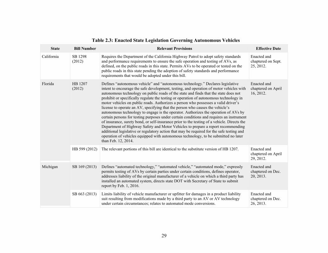
29

Table 2.3: Enacted State Legislation Governing Autonomous Vehicles

State Bill Number Relevant Provisions Effective Date

California SB 1298 (2012)

Requires the Department of the California Highway Patrol to adopt safety standards and performance requirements to ensure the safe operation and testing of AVs, as defined, on the public roads in this state. Permits AVs to be operated or tested on the public roads in this state pending the adoption of safety standards and performance requirements that would be adopted under this bill.

Enacted and chaptered on Sept. 25, 2012.

Florida HB 1207 (2012)

Defines “autonomous vehicle” and “autonomous technology.” Declares legislative intent to encourage the safe development, testing, and operation of motor vehicles with autonomous technology on public roads of the state and finds that the state does not prohibit or specifically regulate the testing or operation of autonomous technology in motor vehicles on public roads. Authorizes a person who possesses a valid driver’s license to operate an AV, specifying that the person who causes the vehicle’s autonomous technology to engage is the operator. Authorizes the operation of AVs by certain persons for testing purposes under certain conditions and requires an instrument of insurance, surety bond, or self-insurance prior to the testing of a vehicle. Directs the Department of Highway Safety and Motor Vehicles to prepare a report recommending additional legislative or regulatory action that may be required for the safe testing and operation of vehicles equipped with autonomous technology, to be submitted no later than Feb. 12, 2014.

Enacted and chaptered on April 16, 2012.

HB 599 (2012) The relevant portions of this bill are identical to the substitute version of HB 1207. Enacted and chaptered on April 29, 2012.

Michigan SB 169 (2013) Defines “automated technology,” “automated vehicle,” “automated mode,” expressly permits testing of AVs by certain parties under certain conditions, defines operator, addresses liability of the original manufacturer of a vehicle on which a third party has installed an automated system, directs state DOT with Secretary of State to submit report by Feb. 1, 2016.

Enacted and chaptered on Dec. 20, 2013.

SB 663 (2013) Limits liability of vehicle manufacturer or upfitter for damages in a product liability suit resulting from modifications made by a third party to an AV or AV technology under certain circumstances; relates to automated mode conversions.

Enacted and chaptered on Dec. 26, 2013.

30

Table 2.3, continued State Bill Number Relevant Provisions Effective Date

Nevada AB 511 (2011) Authorizes operation of AVs and a driver’s license endorsement for operators of AVs. Defines “autonomous vehicle” and directs state Department of Motor Vehicles (DMV) to adopt rules for license endorsement and for operation, including insurance, safety standards and testing.

Enacted and chaptered on June 17, 2011.

SB 140 (2011) Prohibits the use of cell phones or other handheld wireless communications devices while driving in certain circumstances, and makes it a crime to text or read data on a cellular phone while driving. Permits use of such devices for persons in a legally operating AV. These persons are deemed not to be operating a motor vehicle for the purposes of this law.

Enacted and chaptered on June 17, 2011.

SB 313 (2013) Relates to autonomous vehicles. Requires an autonomous vehicle that is being tested on a highway to meet certain conditions relating to a human operator. Requires proof of insurance. Prohibits an autonomous vehicle from being registered in the state, or tested or operated on a highway within the state, unless it meets certain conditions. Provides that the manufacturer of a vehicle that has been converted to be an autonomous vehicle by a third party is immune from liability for certain injuries.

Enacted and chaptered on June 2, 2013.

North Dakota HB 1065 (2015)

Provides for a study of AVs. Includes research into the degree that automated motor vehicles could reduce traffic fatalities and crashes by reducing or eliminating driver error and the degree that automated motor vehicles could reduce congestion and improve fuel economy.

Enacted and chaptered on March 20, 2015.

Tennessee SB 598 (2015) Relates to motor vehicles. Prohibits local governments from banning the use of motor vehicles equipped with autonomous technology.

Enacted and chaptered on April 24, 2015.

31

Table 2.3, continued State Bill Number Relevant Provisions Effective Date

Utah HB 280 Autonomous Vehicle Study

41-26-101. Title. This chapter is known as “Autonomous Vehicles.” Section 2. Section 41-26-102 is enacted to read: 41-26-102. Autonomous motor vehicle study. (1) As used in this section, “autonomous vehicle” means a motor vehicle equipped with technology that allows the motor vehicle to perform one or more driving functions through vehicle automation, without the direct control of the driver. (2) Each agency of the state with regulatory authority impacting autonomous vehicle technology testing shall facilitate and encourage the responsible testing and operation of autonomous vehicle technology within the state. (3) (a) The Department of Public Safety, in consultation with other state agencies, including the Division of Motor Vehicles and the Department of Transportation, shall study, prepare a report, and make recommendations regarding the best practices for regulation of autonomous vehicle technology on Utah highways. The study shall include:

(i) evaluation of standards and best practices suggested by the National Highway Traffic Safety Administration and the American Association of Motor Vehicle Administrators;

(ii) evaluation of appropriate safety features and standards for autonomous vehicles in the unique weather and traffic conditions of Utah;

(iii) evaluation of regulatory strategies and schemes implemented by other states to address autonomous vehicles, including various levels of vehicle automation;

(i) evaluation of federal standards addressing autonomous vehicles; and (ii) recommendations on how the state should address advances in autonomous vehicle technology

through legislation and regulation. (b) The Department of Public Safety shall provide a written report and present findings of the report, including recommendations, to the Transportation Interim Committee and the Public Utilities and Technology Interim Committee, before December 1, 2016. The Division of Motor Vehicles, the Department of Transportation, and the Department of Technology Services shall be present for the report to the Transportation Interim Committee.

(4) The Department of Public Safety, the Division of Motor Vehicles, the Department of Transportation, and the Department of Technology Services may partner and contract with person for the purpose of testing autonomous vehicles within the state.

Enacted and chaptered on March 23, 2016.

Washington, D.C.

2012 DC B 19-0931

Defines “autonomous vehicle” as “a vehicle capable of navigating District roadways and interpreting traffic-control devices without a driver actively operating any of the vehicle’s control systems.” Requires a human driver “prepared to take control of the autonomous vehicle at any moment.” Restricts conversion to recent vehicles, and addresses liability of the original manufacturer of a converted vehicle.

Enacted and effective from April 23, 2013.

Sources: http://www.ncsl.org/research/transportation/autonomous-vehicles-legislation.aspx and http://cyberlaw.stanford.edu/wiki/index.php/Automated_Driving:_Legislative_and_Regulatory_Action#Enacted%20www.utexas.edu

32

Before considering the legislation in individual states, it is first important to underscore the emergence of various national recommendations for unified state oversight of C/AVs. In its 2013 Statement, NHTSA concludes that “states are well suited to address issues such as licensing, driver training, and conditions for operation related to specific types of vehicles” (NHTSA 2013, at 10). It also indicated that it “does not believe that self-driving vehicles are currently ready to be driven on public roads for purposes other than testing.” States are thus encouraged to develop regulations governing C/AV testing and limit the use of self-driving mode to conditions conducive to safe operation on public roadways.

Beyond NHTSA’s promotion of state oversight of testing, licensing, and operation of C/AVs, the ULC (ULC 2014) has garnered significant momentum for a uniform state act adopted across states governing C/AV testing and deployment. Uniformity between states with regard to C/AV operation will not only provide a more predictable market for technological innovation but will also promote ease of commerce between states as C/AVs become increasingly integrated into the transportation system. These and other model laws or frameworks for uniform or model state laws are provided in Appendix G and discussed in more detail in Section 2.6.

Several individual states have also been very active in the oversight of C/AVs. Their legal regimes are discussed below. Yet it is important to note that there is considerable activity in other states as well. As of July 2015, at least 23 states other than Texas were considering legislation to regulate C/AVs modeled largely on the laws already adopted in other states (Gosselin 2015, p.95). One of the simplest proposals—in Connecticut—simply requires that “the general statues be amended to allow the use of AVs for testing purposes, and direct[s] the Department of Motor Vehicles to promulgate regulations concerning the use of such vehicles” H.R. 6344, 2015 Gen. Assemb., Reg. Sess. (Conn. 2015). This brief summary may need to be updated regularly for those interested in following legislation in the states. For example, Florida amended its rules very recently. See below for some of the general changes.

2.2.6 Overview of State Laws Governing C/AVs

State regulations of C/AVs currently run the gamut from authorization to operate AVs on public roads in Nevada, to having regulations on testing but not public use in California, to having no regulation on C/AVs in the vast majority of states. Although the laws vary on important details, most of the states that actively regulate C/AVs generally impose some regulatory oversight of testing and/or deployment of C/AVs operating in the state (Kohler & Colbert-Taylor 2015). A few states also impose other restrictions, such as mandated technologies on C/AV vehicles sold in the states and disclosures for consumers regarding the OEM’s collection of private information after sale of the vehicle.

Testing and Deployment of C/AVs on Public Roadways

As just mentioned, NHTSA recommends states actually regulate the testing and operation of C/AVs on public highways (NHTSA 2013). At least five states explicitly allow C/AVs on at least some public roads only if they meet prescribed criteria (ULC 2014, p. 6). Several states go further and require the issuance of a license or permit as a precondition to operation (Cal. Regs. § 227.04(d); Nev. Regs. § 8.3). Not all states actively regulate testing or distinguish between operating a C/AV for testing versus operating a vehicle for regular deployment, however (e.g., D.C. Code § 2352). Beyond direct oversight of testing, California and Nevada also require

33

disclosure of accidents and near-misses occurring during testing (Cal. Regs. §§ 227.46, 227.48; Nev. Regs § 10.4).

Nevada became the first state to enact legislation on C/AVs in 2011, after passing Assembly Bill (AB) 511, which defined “autonomous vehicle” and directed the state DMV to adopt rules for license endorsement and for operation, including insurance, safety standards, and testing (AB 511 2011). The regulations, first adopted in 2012 and later revised in 2013, require applicants show proof of 10,000 AV operational miles as well as a summary of statistics before being granted a license to test on public roads (Nevada DMV 2013). Nevada within its 2013 amendment to its AV law specified some Level 1, 2, and 3 technologies as not being “autonomous,” noting that autonomous technology means:

technology which is installed on a motor vehicle and which has the capability to drive the motor vehicle without the active control or monitoring of a human operator. The term does not include an active safety system or a system for driver assistance, including, without limitation, a system to provide electronic blind spot detection, crash avoidance, emergency braking, parking assistance, adaptive cruise control, lane keeping assistance, lane departure warning, or traffic jam and queuing assistance, unless any such system, alone or in combination with any other system, enables the vehicle on which the system is installed to be driven without the active control or monitoring of a human operator (Nev. SB 313, 2013).

Testing licenses in Nevada are predetermined and limited to specific geographic zones, although these may be enlarged (Nev. Rev. State. § 482A.120). General requirements that span across all AV testing in Nevada include having two persons physically in the vehicle while testing, including one person in the driver’s seat who is able to take control (Nevada DMV 2013).

After testing is successful, the deployment of an AV is allowed in Nevada only after issuance of a “certificate of compliance,” issued by the manufacturer or a registered sales facility. The certificate can be issued only if the vehicle meets requirements set forth in Nevada regulations (Nev. Regs. § 16).

California legislation and regulation provides similar types of oversight for AV testing and deployment. In contrast to Nevada, however, testing on AVs can occur on all roads in the states. Like Nevada, however, vehicle manufacturers must obtain a testing permit from the DMV and comply with permit requirements when testing AVs on California roads (California DMV 2012). California DMV requirements for manufacturer testing include registering the AV with the DMV, completing previous AV testing under controlled conditions, using qualified test drivers who sit in the driver’s seat with the ability to take control of the AV, and a $5 million insurance or surety bond maintained by the manufacturer (CA Vehicle Code 38570(A)(5)). In order to deploy a vehicle in California after testing, the vehicle must be approved by the Calif. DMV. A majority of the California’s efforts are rooted in a close working relationship between the California Department of Transportation (Caltrans), the California DMV, and the California Partners for Advanced Transit and Highways (PATH) of the University of California, Institute of Transportation Studies. PATH and Caltrans primarily focus on efforts for cooperative adaptive cruise control, automated truck platooning, and vehicle-assist and automation applications for full-size public transit buses (PATH 2014).

Florida adopts some of the provisions of Nevada law, but the State exerts considerably less control over manufacturers wishing to test AVs on public roadways and places no geographical restrictions on that testing. “In Florida, when a testing entity presents insurance to the Department and pays the title fees, the Department will brand the vehicle title ‘autonomous’ and ‘autonomous

34

vehicle’ will print on the registration certificate” (Florida DHSMV 2014, p. 5). Thus, although there are certain standards required of AVs tested or deployed in the State, including a $5 million proof of insurance and vehicle certification, “the Department does not require an application or otherwise regulate the testing entity.” The Department also does not have the authority to deny a request to test AVs in the State. Florida amended its legislation in July 2016.

Michigan allows C/AV testing so long as the vehicle is operated by an authorized agent of the manufacturer, and an individual is present in the vehicle and able to take control immediately if necessary. But the State specifically bans operation of AVs for non-testing purposes (Mich. Comp. Laws §§ 257.663, 665). Tennessee legislation, by contrast, prohibits any political subdivision of the state from prohibiting the use of an AV so long as the vehicle complies with all safety regulations of the political subdivision (SB 598 2015).

Taking a slightly different approach, the District of Columbia enacted the Autonomous Vehicle Act of 2012, which expressly allows the operation of AVs on District roadways (D.C. Code §§ 50-2351 to -2354). The District requires only that a vehicle must have a manual override and a driver in the driver’s seat ready to take over, and operate in compliance with the District regulations, D.C.’s other normal traffic laws and regulations (§50-2351). Rules to implement the law are being promulgated by the DMV, including procedures for registration and issuance of permits to operate AVs (Kohler & Colbert-Taylor 2015, p.117).

In 2015, both Arizona (EO 2015) and Virginia announced their decision to move forward with research and development of AV operations. In Arizona, Governor Doug Ducey signed Executive Order (EO) 2015-09 in August directing various agencies to “undertake any necessary steps to support the testing and operation of self-driving vehicles on public roads within Arizona” (Ducey 2015). The EO establishes the Self-Driving Vehicle Oversight Committee within the governor’s office to develop regulations for enabling the development and operations of AV pilot programs at selected universities.

Utah in May 2016 authorized an autonomous motor vehicle study. HB 280 authorized each agency of the state with regulatory authority impacting autonomous vehicle technology testing shall facilitate and encourage the responsible testing and operation of autonomous vehicle technology within the state. The bill authorizes that the department s of Public Safety, Motor vehicles, Transportation and Technology Services can contract and partner with groups for testing autonomous vehicles in the state. The Department of Public Safety, in consultation with other state agencies, including the Division of Motor Vehicles and the Department of Transportation, shall study, prepare a report, and make recommendations regarding the best practices for regulation of autonomous vehicle technology on Utah highways. The study shall include:

(i) evaluation of standards and best practices suggested by the National Highway Traffic Safety Administration and the American Association of Motor Vehicle Administrators;

(ii) evaluation of appropriate safety features and standards for autonomous vehicles in the unique weather and traffic conditions of Utah;

(iii) evaluation of regulatory strategies and schemes implemented by other states to address autonomous vehicles, including various levels of vehicle automation;

(iv) evaluation of federal standards addressing autonomous vehicles; and (v) recommendations on how the state should address advances in autonomous vehicle

technology through legislation and regulation.

35

A report is due in December 2016 to house and senate committees that includes recommendations and findings

Vehicle Requirements

NHTSA and the ULC both endorse several basic design features in AVs used for testing or deployment. These include a device that allows for quick disengagement from automated mode; a device that indicates to others whether the vehicle is operating in automated mode; and a system to warn the operator of malfunctions (ULC 2014, p.9). Several state laws include one or all of these requirements for AVs sold in the state. These states include California, Florida, D.C., and Nevada (ULC 2014 p. 9-10).

Individual states have also imposed other requirements. Nevada has required that EDRs capture data 30 seconds before a collision in AVs, and preserve the data for 3 years (Nevada DMV 2014). Similarly, the District of Columbia’s DMV issued guidelines in June 2014 that require that EDRs be completely separate from all other data systems, must provide data in a read-only format when requested, and must retain all data for at least 3 years following a collision (District of Columbia DMV 2014). California also requires a crash data recorder for AVs sold to the public and the State imposes detailed requirements governing the capabilities of the recorders (Cal. Vehicle code § 38750(c)(1)(G)).

Operator Requirements

NHTSA recommends that an endorsement or separate driver’s license should be issued for operators of C/AVs certifying that the operator has passed a test concerning safe operation of the C/AV or completed a certain amount of hours operating the vehicle (NHTSA 2013).

Consistent with NHTSA’s recommendations, both Michigan and Nevada testing regulations for AVs require a special driver’s license certification and license plates (Nev. Admin. Code §§ 482A.040, .050, .110 (2014)). Nevada, the first state to enact AV legislation, has only briefly addressed private individuals as operators as AVs, stating that “[w]hen autonomous vehicles are eventually made available for public use, motorists will be required to obtain a special driver license endorsement and the DMV will issue green license plates for the vehicles.”

California lays out detailed requirements for a AV driver test: the manufacturer must identify the operator in writing to the DMV; the operator must have been licensed to drive a motor vehicle for at least 3 years immediately preceding application, and can provide proof that during that time that the operator did not have more than one violation of specific sections of the vehicle code (Cal. Regs. §§ 227.18, 227.20). The AV operator must also have completed the manufacturer’s AV training program, which includes, but is not limited to, instructions on AV technology and defensive driver training (California DMV 2012).

Clarification of Liability Standards and Insurance Requirements Several states impose special insurance requirements on C/AVs before they can be tested

or deployed on public roads. Both California and Nevada, for example, impose a $1–5 million insurance requirement before allowing testing of AVs on public roads (Cal. Vehicle Code § 3875(b)(3); Nev. Regs. § 8.4; Fla. Stat. § 316.86). Michigan, by contrast, does not impose additional insurance requirements on AVs for testing or deployment purposes (Mich. Comp. Laws § 257.665(1)).

36

Florida, Nevada, and the District of Columbia have liability protection for post-sale conversion of vehicles to AVs (Boske and Harrison 2014). Liability protection is given to OEMs whose vehicles are converted to C/AVs. California, however, has no explicit mention of such liability protection.

2.2.7 International Developments

There has been considerable interest in regulating and encouraging C/AV technology abroad. In Europe, generally speaking, much of the push for research and development of autonomous driving technologies comes from a desire for competitiveness and to reap the benefits of the technology in European transportation systems. CVs are also very much a point of interest for transportation technology developers and policy makers on the continent. Some national governments have delved into the idea of autonomous driving by funding studies, but most of the large-scale research has been done at the EU level through multiple projects focusing on a variety of topics.

As in the US, there is no union/national legislation or policy regarding AVs in the EU. Thus, just as individual states have been the primary regulators overseeing the operation of C/AVs in the US, in Europe special permits, typically awarded by local and/or regional authorities, have allowed most of the research and development to occur (Kim et al. 2014). A few member states in the EU have made progress developing and implementing policies regarding AVs, but most still fall short of truly enabling their testing and development.

Many proponents for autonomous driving in Europe claim that the Vienna Convention on Road Traffic was the greatest obstacle preventing a more robust approach to the development and adoption of these technologies. In Article 8, the Convention used language that incidentally prevented the serious development and testing of AVs, such as “Every driver shall at all times be able to control his vehicle” (Economic Commission on Europe 1968). Still, technological breakthroughs were occurring despite the belief that this section of the convention was deleterious to AVs’ progress.

As greater concern mounted about Europe’s lack of contribution to the progression of autonomous driving, EU member states began to consider how they could move past the challenges they were facing. As more conversations were facilitated, it became clear that the primary catalysts for the development of AVs in Europe were competitiveness, sustainability, efficiency and harmonization between national borders, low carbon levels, and, to a lesser degree, safety (Schreus et al. 2015). Finally, after the governments of Germany, Italy, France, Belgium, and Austria submitted an amendment, the United Nations amended the Convention on Road traffic to allow drivers to take their hands off the wheel of self-driving cars (SafeCarNews 2014). This is a significant development for autonomous driving and autonomous technological development, because arguably the greatest obstacle was removed and development of beneficial policies regarding AVs can now be explored more aggressively.

2.2.8 EU Initiatives

The largest and most publicized EU foray into autonomous driving seems to be the CityMobile2 project, which began in 2012. CityMobile2 is an AV project providing public transit that is funded by the EU’s Seventh Framework Programme for Research and Development of Various Technologies (CityMobile2 2015). The project has operated demonstrations in a handful of EU member states with La Rachelle, France receiving most of the attention. The technology is

37

still in the early stages of development and policy and legal questions seem to have kept the project from being implemented more quickly. There is currently no policy regarding AVs in France, so the project team has been in close conversation with French authorities to gain permission for such vehicles. The conversations and feedback from both parties resulted in the Transport Minister authorizing CityMobile2 (CityMobile2 2015).

The EU is also providing funding for research on autonomous driving, most notably through European Commission projects aimed at keeping the Union competitive from a market perspective. The European Commission Directorate General for Communications Networks, Content & Technology, also known as DG Connect, is an organization within the European Commission that researches ITS and also supports research in the area of automated mobility. DG Connect is also associated with the autonomous driving forum called iMobility and forwards readers to the forum’s website when searching for automated driving. Moreover, the EU now provides a platform called FUTURIUM for debating the future and trajectory of autonomous driving on the continent (Schreus et al. 2015). Although none of these initiatives are explicitly for the purpose of developing autonomous driving policies or regulations, they are worth noting if only for the sake of acknowledging the EU’s recognition of potentially serious changes coming to the transportation field.

EU Member States

A number of individual countries are seeking to enable research and develop within their borders. Below are examples of the most prominent initiatives.

Sweden

“Drive Me”—Self-Driving Cars for Sustainable Mobility is the first large-scale autonomous driving project being undertaken in Gothenburg, Sweden. The collaborative project between Volvo, the Swedish Transport Administration, the Swedish Transport Agency, Lindholmen Science Park, and the City of Gothenburg will have 100 vehicles driving autonomously on the city’s public roads (Swedish Transport Administration 2015). This is a solid breakthrough as much of the testing of self-driving vehicles in Europe has been done on private roads. Sweden has also been at the forefront of studying CVs with its SARTRE Project. The Safe Road Trains for the Environment project is funded by the European Commission under the Framework 7 program and aims to develop strategies and technologies to have platooning vehicles on public highways (SARTRE 2015). Government and industry are excited about greater transport efficiency and safety to be gained from platooning.

Germany

AutoNOMOS Labs is a project at the Freie Universität Berlin that researches and develops autonomous and driver-assistance technologies (Autonomos Labs, not dated). The Stadtpilot is another research project that seeks to develop autonomous technologies and test them in real city traffic (Technische Univesität Braunschweig 2010). From a policy perspective, the German Transport Ministry is pushing the conversations about autonomous driving at the national level. They hold round table meetings with members from various transportation stakeholder groups twice a year to address the issues, in addition to assembling working groups to take a look at policy and legal questions (Schreus et al. 2015). The hope is that they will reach a much better understanding of the features that both benefit and hinder the eventual adoption of AVs. Germany

38

seeks to be a leader in developing policy for AVs and the country hopes to provide an environment for its many automakers to capitalize on this potential market.

UK

The UK government has contributed to research and has begun studying various facets of autonomous driving. On July 30, 2014, the government created a “driverless cars” competition and encouraged individual municipalities to work with technology developers to test their vehicles in their cities. In February 2015, the Department of Transport released a summary report and action plan for how to handle autonomous driving by creating a Code of Practice. The proposed idea of the Code of Practice is intended to promote safety and set clear guidelines for responsible testing (Department of Transport 2015). Still, many feel that the UK government has been lethargic in its attempt to facilitate the reality of autonomous driving.

France

The French government is working to develop AVs through its program to make the country a leader in industry and technology. Launched by the “New Industrial France” program, self-driving cars will be on public roads in 2015. This project is being overseen by the French Ministry of Finance and should have its first implementation at the global ITS show for smart transport (Sustainable Mobility 2015). French researchers have also studied and developed the AV called the Renault Espace by modifying a Renault Grand Espace to be self-driving (Kurzweil 2015). However, this vehicle is geared primarily for research, and not large-scale public use due to its bulky robotic driving system.

Japan

In 1996, Japan began its progression to the utilization of AVs with the Advanced Cruise-Assist Highway System (AHS) Research Association demonstrating the convoying of vehicles. Since then, a number of companies have sought to bring greater autonomy to the country’s roads.

The government of Japan became serious about the development of AVs when it began to research how these vehicles might be developed and welcomed on public infrastructure. A number of government ministries are now working together to effectuate AVs on Japanese roads and the government has defined four levels of vehicle autonomy in much the same way that NHTSA has (Japan Ministry of Economy 2014), in an effort to help catalyze greater conversation about autonomous driving and begin to frame the self-driving conversation.

Work has been done to make provisions for AV technologies, although there is still no classification of driver’s license for these vehicles. However, in 2013, Nissan’s AV Leaf was given an AV license plate and allowed to operate on Japanese roads (Motherboard 2013). This is in line with the company’s desire to have multiple vehicles operating autonomously on Japanese roads by 2020. The catch, however, is that this vehicle is not completely autonomous but rather utilizes autonomous driving features. This is fairly similar to Cadillac’s semi-autonomous technology called “Super Cruise.” The technologies offer autonomous features but fall short of providing totally self-driving cars. Still, this is just one example of progress being made toward a more autonomous driving environment.

The Ministry of Land, Infrastructure, Transport and Tourism (MLIT) has also spelled out other ways of pursuing autonomous driving in the country. They are seeking to move the direction of Japanese ITS toward autonomous technologies with the ultimate goal of reaching autopilot or

39

Level 4 autonomy in the early 2020s (MLIT 2012). The MLIT created an Autopilot System Study Group to dive deeper into the idea of AVs. They looked at some of the issues with self-driving vehicles and studied potential policies that would be appropriate for enabling AVs. “Autopilot” driving demonstrations also occurred at CEATEC Japan and at the ITS World Congress in 2013 (Yamamoto 2015). These technologies are still being developed and will likely not be realized by the public for years to come.

The Japanese government also plans to pursue AV opportunities through public-private partnerships. This is particularly appropriate since major automobile companies like Nissan, Subaru, Mazda, Toyota, and Honda are located in the country. The government clearly sees an opportunity for the private markets to push for greater progress and innovation with companies that already inherently seek to do this. The government only needs to ensure that infrastructure and policies are in place to make the transition and adoption as seamless as possible. Together, Japanese private and public sectors will invest a total of 10 billion yen ($83.4 million) to build facilities for testing these technologies (Nikkei 2014). However, it still appears that the majority of the breakthrough is coming from the private sector with companies like Nissan, Toyota, and Honda seeking to truly push the envelope on AV development. This commercial viewpoint is hoping to capitalize on a few potential markets, not the least of which is the aging population in the island country.

The Japanese Council for Science, Technology and Innovation (JCSTI) has also sought to address AVs in a proactive way. In November of 2014, the CSTI, Japanese Cabinet Office, and Cross-Ministerial Strategic Innovation Promotion Program, organized a workshop on C/AVs. The scope of the discussions included technologies, human factors, legal issues, and integrated applications of automated driving technologies, such as reduction of traffic injuries and next generation transportation services (JCSTI 2014). Considering these ideas will help the national government create autonomous driving policies and regulations that will benefit the AV industry and the public. The Cross-Ministerial Strategic Innovation Promotion Program is another Japanese government project that is researching autonomous driving (JCSTI 2014).

In the future, Japanese authorities intend to implement multimodal transportation systems centered on pedestrian utility. Policymakers believe AVs will be a supplement to these networks and create safer and more time-efficient transport options (JCSTI 2014). However, Japanese legislation is still fairly prohibitive of vehicle autonomy, save for the authorized exceptions (i.e., Nissan Autonomous Leaf). The Road Traffic Act requires drivers to ensure safety at all times while the car is being driven (Nikkei 2015). It’s clear how this requirement can be problematic for the potential of self-driving cars and it’s fairly similar to the pre-amended Vienna Convention. Time will tell if Japan seeks to amend its regulations in the same way the EU member states lobbied for the new Convention on Road Traffic.

Canada

In Canada, no federal laws have yet been passed regarding AVs. The Government of Ontario has launched a pilot program for testing vehicles on Ontario’s roads. On January 1, 2016, Ontario will allow the testing of vehicles and related technology on their roads. According to the Ministry of Transportation in Ontario (MTO), this step will promote research and development by the 100 companies and institutions involved in the C/AV industry (Government of Ontario, October 2015).

The proposed pilot framework prescribed conditions to facilitate the testing of AVs for the next 5 years (Government of Ontario 2013).

40

While in autonomous mode, vehicles will be subject to these regulations:

• Restricted use for testing purposes only;

• A driver must be present in the vehicle at all times and have a valid G class driver’s license;

• Driver must be trained to safely operate an autonomously equipped vehicle;

• Driver must remain seated in the driver’s seat at all times monitoring the safe operation of the AV, and be capable of taking over immediate manual control; and

• May only be operated by those drivers approved by the ministry (i.e., employed by the manufacturers, software developers, etc.) and for testing purposes only.

Current Highway Traffic Act rules of the road and penalties will apply to the driver/vehicle

owner. The AV must display signs at the front and rear to show that it is an AV; and the pilot program will employ a phased-in approach that initially limits driving exposure (e.g., specific roads, posted speed limits, traffic volumes, etc.).

For registration and insurance, proof of third-party liability insurance, in an amount not yet determined, will be needed. In addition, vehicles are subject to these requirements:

• They must be registered and plated as a passenger vehicle for use in Ontario;

• Only vehicles manufactured and equipped by recognized parties permitted;

• Operator must submit an application to MTO for approval before vehicle permit and number plates for the AV are issued;

• Extensive supporting documentation will have to be submitted with the application, including but not limited to: (i) proof of ownership of the vehicle; (ii) certification by the owner that the AV meets all of the usual provincial and federal

safety standards that are applicable to motor vehicles, and that the autonomous technology does not diminish any of the required safety features;

(iii) verification that the AV is not a homebuilt conversion; (iv) agreement by the registrant to provide any driver with sufficient training in the

operation of AVs; (v) agreement by the registrant that the AV will be operated for testing purposes only; (vi) certification by the owner the AV has desirable safety features, including, but

limited to: (a) a mechanism to quickly disengage the autonomous technology, so that the

driver can take over manually at any time; (b) an indicator that shows when the vehicle is in its autonomous mode; (c) a system to alert the drive if the autonomous technology fails, or unexpectedly

turns off; (d) a mechanism to capture and store any data about the prior operation of the

vehicle from at least 30 seconds before any collision (Government of Ontario 2013).

41

The government noted that information on applying for the pilot application would be released during late November 2015.

Australia

The Government of South Australia introduced legislation for on-road testing of AVs in September 2015 (Government of South Australia: Attorney General’s Office 2015). The Motor Vehicles (Trials of Automotive Technologies) Amendment Bill will provide for exemptions from existing laws to allow trials of AVs on public roads. Amendments include a change in the definition of uninsured motor vehicle; insertion of a new section for trials of automotive technologies; authorization for the Minister of Transport to issue, publish, and adopt guidelines; and authorization for the Minister of Transport to authorize trials of automotive technologies.

The Bill requires the Minister to report to Parliament within 6 months of the completion of an authorized trial and to prepare a report in relation to the authorized trial (HA GP 334-B OPC 12 September 23, 2015 (Government of South Australia: DPTI 2015). Australia will test AVs during November 2015 (ABC 2015) for the first time. Volvo will be conducting testing in Adelaide’s southern suburbs on the Southern Expressway on November 7 and 8, 2015. There will be multiple vehicles, with Volvo bringing the XC90 model used in Sweden’s DriveMe project. The vehicles will test overtaking, lane changing, emergency braking, and the use of on and off ramps.

2.2.9 Industry Association Activity

There are also private industry standards that bear on C/AV technology. The International Organization for Standardization (ISO) has set many standards utilized the world over. In 2014, the ISO Technical Committee for Road Vehicles (ISO/TC22) began work to develop standards related to different kinds of AVs (ISO, 106: 2014).

The SAE has an On-Road Automated Vehicle Standards Committee that released a new standard (J3016) in January 2014 titled Taxonomy and Definitions for Terms Related to On-Road Motor Vehicle Automated Driving Systems. The standard provides a common taxonomy and definitions for automated driving with a goal to simplify communication and facilitate collaboration within and across policy domains. A dozen key terms were defined. Figure 2.3 summarizes J3016 (SAE 20014). The Committee began working on J3092, Dynamic Test Procedures for Verification and Validation of Automated Driving Systems, in March 2015. Another item the committee has issued is J3018, Guidelines for Safe On-Road Testing of SAE Level 3, 4 and 5 Prototype Automated Driving Systems, which was released in March 2015.

42

Figure 2.3: SAE International’s Definitions of Autonomous Vehicle Levels (J3016 Standard)

2.3 The Legality of C/AVs in Texas: Licensing and Related Issues

Texas has not yet passed laws or regulations that regulate C/AV use directly. This section thus considers the existing law—all of it developed without C/AVs in mind—that nevertheless will serve to regulate this new technology as it is assimilated into the State.

The operation of C/AVs on Texas roadways is likely to intersect with existing Texas law in two overlapping ways. The first is governed by legislation that identifies who can operate vehicles in Texas and the responsibility of these owners for violations. The second involves rules of the road and other practical constraints on the operation of vehicles.5

2.3.1 Operation of Motor Vehicles in Texas

While there are ambiguities, the most plausible reading of the Texas Motor Vehicle Code with respect to C/AVs is that to be operated legally on Texas roadways, each vehicle must have an identified and legally responsible human operator with a valid driver’s license. Specifically, the 5 As noted earlier, the technologies themselves are not so clearly distinct that the differences between Autonomous Vehicle and Connected Vehicle have legal relevance. Rather than an artificial parsing of CV vs. AV – which simply can’t be done at present in most areas of the analysis – we take a broad view of the technologies to ensure a more comprehensive assessment of the emerging law/policy. Where there are meaningful distinctions to be drawn with regard to the law and CVs vs. AVs, these are drawn out within sections 3 through 5.

43

general structure of the Texas Motor Vehicle Code places full responsibility on “operators” of vehicles to comply with all Code requirements, rules of the road, and other laws. While “operators” are defined as “persons” who need not be humans by definition (Texas Transportation Code § 541.001(4)), these “persons” must nevertheless obtain a drivers’ license in order to operate a vehicle on a highway in the state (§ 521.021). Existing driver’s license requirements, moreover, include a number of requirements (e.g., thumbprint; photo; signature; residence) (§ 521.121) that can only be satisfied, as currently designed, by humans.

Although this licensed “operator” need not be actively driving the vehicle, the most plausible interpretation of the statute does demand the “operator” to at least be present in the vehicle while it is moving in order to be in compliance with the law. Violations of the Code, moreover, fall on the licensed “operator” of the vehicle, although they can be imposed jointly on other operators as well.

Despite a relatively clear structure that seems to tolerate the operation of C/AVs on Texas roadways, there are nevertheless gaps and ambiguities in the law regarding the legality of 1) vehicles without a designated operator; 2) the operator’s physical role in operating the vehicle; 3) non-human “operators”; and 4) the ultimate legal responsibility for violations. Each is discussed in turn.

Vehicles Without a Designated Operator

Numerous responsibilities and requirements attach to the “operator” of a motor vehicle, but there does not appear to be the critical legal link in Texas Law that prohibits vehicles from “moving” on Texas roadways unless they are being moved by an “operator” (“persons” cannot “operate” a vehicle without a driver’s license [§ 521.021], but presumably vehicles can move without being controlled by persons). One could argue, then, that driverless cars are legal without a designated “operator” aboard the vehicle or even remotely controlling the vehicle.

Such a literal interpretation of the Texas Motor Vehicle is likely to be unpersuasive, however. First, the bulk of the Motor Vehicle code and drivers’ handbook prescribes requirements, rules of the road, and other operation requirements for “operators” (see, e.g., §§ 545.151, 542.4045, 544.008, 544.010, 545.051, 545.052, 545.062). The interpretation that some vehicles can operate without “operators” would thus exempt those vehicles from virtually all of the applicable rules of the road and related operational requirements. Vehicles with operators, in other words, would be subject to hundreds of specific requirements; driverless cars, by contrast, would need only ensure that they are not driven in ways that are “unsafe” (§ 547.004(a)). Additionally, the prohibition that an “operator” may not leave a car “unattended” without first stopping the vehicle completely would make little sense if other vehicles could move freely without operators (§ 545.404). Finally, in criminal interpretations of the Texas Code, the courts have held persons liable for “operating” cars if they are started, even if they are idling.6

A much more plausible interpretation of the Motor Vehicle Code as applied to C/AVs, then, is that each vehicle that moves on the roadways must be controlled by an identified “operator,” and that under current law to be “authorized, this “operator” must have a drivers’

6 See Denton v. State, 911 S.W.2d 388,389 (Tex.Crim.App. 1995) (finding that starting the ignition and revving the accelerator was sufficient to find that defendant “operated” the vehicle as an element in “Unauthorized Use” charge required) but see Texas Dept. of Public Safety v. Allocca, 301 S.W.3d 364 (Tex.App.-Austin) (sleeping defendant in driver’s seat parked legally on private property does not provide “probable cause” to believe that the vehicle had been previously operated).

44

license. The licensed “operator,” in turn, is responsible for compliance with the Motor Code and other rules of the road. This obligation falls on the operator and not on the vehicle. Moreover, if there is no identifiable “operator” present in a vehicle (authorized or unauthorized per the criminal code), the vehicle could presumably be confiscated (e.g., § 545.305).

Designated Operator’s Role in Physical Operators

Even if each vehicle moving on State highways must be operated by a licensed “operator,” there is still the open question of whether that operator actually needs to be steering or controlling the vehicle at all times, as well as whether the operator needs to be physically present in the vehicle. Both issues remain somewhat ambiguous under current law, although our reading of the law and associated case law suggests that current law allows operators to be at least partly inattentive, provided they are in control in the vehicle. By contrast, Texas law can be read to preclude driverless cars controlled remotely by licensed operators, although greater legal clarity would help reinforce this or the opposite interpretation.

The Inattentive Operator

Texas law defines the “operator” of a vehicle to be that person “who drives or has physical control of a vehicle” (§ 541.001(a)). The definition of “operator” seems to allow for the possibility that this person may not be operating the vehicle per se but has ultimate “physical control” (e.g., “hand-off” to human operator) of the vehicle.

Texas law thus currently seems to allow an operator to be present in the vehicle, but not necessarily in constant control of the vehicle. The Motor Vehicle Code imposes visibility requirements on that operator—they must be able to see the road (§ 545.417), and have a view of approaching traffic at intersections (§ 544.010(c)). But presumably one can comply with these requirements and still allow the “operator” to turn the actual operation over to an automated process.

The Remote Operator

Current law seems to require that “operators” must be present in the vehicle while it is moving, although this requirement is somewhat ambiguous. Speaking most directly to this point is the Texas Transportation Code requirement that operators cannot leave vehicles “unattended” unless they come to a complete stop, with keys removed, etc. (§ 545.404). The common sense meaning of this provision (see Tx. Gvt. Code § 311.011) is that vehicles are not allowed to move unless an operator is present in the vehicle. While it is possible that the term “unattended” could be interpreted to exclude remote operators of AVs or perhaps even to allow AVs to also count as “operators” (§ 545.002) so that the vehicle is in fact not unattended, such interpretations strain the common sense thrust of § 545.404 and at the very least would benefit from some clarifying regulatory guidance or regulatory interpretation.

In addition, at least one other section also places responsibilities on “operators” in ways that appear to require that the “operator” be present in the vehicle; see, e.g., § 550.021 (operator requirements in emergencies), § 550.023 (duty to render aid), and § 550.024 (duty on striking unattended vehicle to find and notify the vehicle’s operator or leave note). This section may also be interpreted to allow the “vehicle” to be designated as a supplemental “operator” capable of fulfilling the emergency operations through software and related technological capabilities, but this again strains common sense.

45

Non-human Operators

The Texas Motor Vehicle Code explicitly lists “operators” as “persons” (§ 541.001(1)), which in turn means “an individual, firm, partnership, association, or corporation” (id. at §541.001)(4)).7 At first blush, then, Texas law would seem to allow OEMs and other commercial entities to be “operators;” humans are not required.

However, this broad interpretation of the legality of a non-human operator is undermined by the Code’s prohibition of a “person” operating “a motor vehicle on a highway in this state unless the person holds a driver’s license issued under this chapter” (§521.021). Thus, while it would seem that non-humans can be operators in the State, the license requirements as currently drafted exclude that possibility by requiring a license and then conditioning these license requirements on a variety of “human” demands (e.g., photos, thumbprints, etc.) (§ 521.121).

It is possible that Texas’s reciprocity with regard to the licensing requirements of other states would allow non-human operators to operate vehicles in the State (§ 521.030). For example, if Nevada provides drivers’ licenses to non-human operators of driverless vehicles, then provided there is a person associated with that license, this vehicle would presumably be legal on Texas roads.

Legal Responsibility for Violation

Although it seems most likely that all vehicles in operation in the State will have a licensed “operator” present in the vehicle, there remains the possibility that in cases of violations—e.g., speeding, crashes involving the violation of rules of the road, etc.—the licensed “operator” can argue the manufacturer is a second operator who should be held responsible for the violation. Enforcement personnel will inevitably confront the possibility of facing two “operators”—one a licensed human present in the car and the other a manufacturer (also a “person” exerting some “physical control” of the vehicle)—both of which point the finger at the other with respect to responsibility for violations (e.g., Glancy et al. 2015 p.52).

Texas law provides for the possibility that multiple parties can be jointly responsible for violations of the Code, but it does not appear to allow the responsibility of the licensed operator to be avoided by shifting responsibility to other supplemental operators. Section 542.302, for example, holds owners or others directing the operation of the vehicle liable for violations of law; however, this section does not suggest that these owners’ responsibility supplant the responsibility of the primary, licensed operator (e.g., § 547.004—“a person commits an offense that is a misdemeanor if the person operates or moves or, as an owner, knowingly permits another to operate or move, a vehicle that: 1) is unsafe so as to endanger a person”). Rather, a common sense interpretation suggests that both owners and operators can simultaneously be responsible for

7 The Texas Code also “include[s]” within the “operator” category the vehicle itself in certain situations (§ 545.002). This could be read to imply that a “vehicle” can be the official “operator” and that the license requirements are not always applicable. A careful reading of the text, however, signals that this added entity is supplemental “operator” and not a substitute “operator.” Specifically the section states that “a reference to an operator includes a reference to the vehicle operated by the operator if the reference imposes a duty or provides a limitation.” By its explicit terms, then, vehicles or other nonhumans do not supplant the “licensed person” as “operator;” the vehicles are only “included” within the “operator” definition in certain circumstances.

46

violations.8 However, Texas law does appear to place responsibility only on those operators performing an act; thus, there remains the possibility that an operator can escape liability this way (e.g., §542.302 (assigns owners or employers with violations if they knew of or directed the violation)).

2.3.2 Rules of the Road and Related Requirements on C/AVs

Rules of the road present some relatively minor legal impediments to the smooth deployment of C/AVs in the state.

Rules of the Road

There are a few rules of the road that may restrict the operation of C/AVs, although the C/AV technology may ultimately be capable of meeting these requirements. For example, special requirements apply to operators in the presence of “emergency vehicles” ((§ 545.156(a) and when following “school buses” that stop (§ 545.066)). The safety signals to stop or pass can include auditory and hand signals (id). Moreover, the appropriate operator response—e.g., yielding or pulling over to the side of the road until the vehicle has passed—may require some operator control. C/AVs will need to ensure compliance with these rules of the road to avoid violations and accidents, either through handoffs or other automated capabilities.

In several other settings, Texas law permits the use of auditory signals and temporary speed signs and traffic signals (e.g., for worker zones). See, e.g., Texas Driver Handbook, Sept. 2014, p.38 (governing temporary signals); p.35 (governing railroad crossings). C/AVs again would need to be equipped to either hand off control in settings with these temporary or auditory signals or be prepared to navigate in automated mode despite these alternate types of signals.

Texas law also assigns considerable driver discretion at right-of-way intersections (id., TDH, p.22). C/AVs may again require careful programming to ensure not only that the right-of-way is gauged correctly given the rules of the road, but also to do so defensively given the likely driver errors that may arise with vehicles that are not automated (e.g., mis-gauging one’s proper place in the queue).

Safety Inspections Required for Registration

Texas law requires that steering systems be inspected in all vehicles. The Texas Department of Public Safety’s criteria require the inspector to have the capability to turn any motor vehicle’s wheel to pass inspection (Tx Department of Public Safety, Vehicle Inspection Chapter 4). As long as C/AVs operate with steering wheels, this requirement will not be an impediment. But for vehicles without steering wheels, the Code requirements may need to be amended to permit vehicles without traditional steering wheels.

Legal Operation of Truck Platoons

There are several ways that truck platoons may violate existing Texas law. These include not providing adequate following distance; moving without an operator in each vehicle; and

8 Reinforcing this interpretation is a provision that includes in the definition of “operator” the “vehicle” in certain settings. § 545.002. The section broadens the definition of “operator” but does so in a way that implies not that only one party can ultimately be held responsible but the reverse.

47

operating in the passing lane. Texas A&M Transportation Institute (TTI) has conducted a study specifically addressing the broader legal impediments to the use of truck platoons in Texas, including added legal restraints imposed by Federal Motor Vehicle Safety Standards (FMVSS) and FMCSA; readers are referred to that project (authored by Jason Wagner in August 2015) for a more focused analysis.9

Many and perhaps most of these legal conflicts can be ameliorated if truck platoons are equated to “tow” trucks, with each truck in the sequence treated as a vehicle in the tow line. In the case of towing, “an operator of a truck or of a motor vehicle drawing another vehicle who is on a roadway outside a business or residential district” can be treated as a single unit (§ 545.062). Treating platoons as a towing operation with multiple vehicles allows for the following legal accommodations:

• Licensed Operators on a Vehicle. If truck platoons consist of a first, operator-controlled vehicle that is connected to “towed” vehicles, then a licensed operator need only be present in the first truck that is doing the towing. Subsequent vehicles in the platoon without operators would not technically be in violation of Texas Law; since they are towed, they are presumably not “unattended” under Section § 545.404.

• Following Distance. The requirement of a following distance that allows for sufficient space between vehicles to allow passing (see § 545.062(c)) will not apply if the vehicles in the platoon are being towed by the lead truck.

However, even if truck platoons are treated as towing operations, some legal ambiguities

and impediments may remain that need to be addressed:

• Trucks (often) prohibited in passing lane. Under Texas rules of the road, trucks are generally not allowed in the passing lanes. This prohibition would thus need to be amended to allow for a third, restricted lane for platoons (Benning 2013). Restrictions imposed by localities (e.g., prohibiting towing trucks from driving in passing lanes) may also need to be amended.

• Multiple vehicles in a “tow.” Since the Transportation Code refers only to a single “vehicle” being drawn behind the first, a clarification may be needed to allow for the towing of multiple vehicles (e.g., truck platoon).

• Merging. Any existing restrictions on merging by towing vehicles or other oversized trucks may also need to be revisited to allow for truck platoons, although we were not able to locate any specific restrictions in place at the statewide level.

2.4 Tort Liability

There is a general consensus that the common law liability rules developed through tort law are well-suited to assimilate C/AV technology in apportioning legal liability for crashes (Anderson et al. 2014; Brookings 2014; and Kalra et al. 2009). After providing a brief orientation 9 Since the instant project consists of a larger mapping project, potential obstacles and conflicts are highlighted at a general level. Fortunately, with respect to the very important topic of truck platoons, TxDOT has already commissioned a more focused study of the intersection between truck platoons and Texas law. Our analysis provides only a reconnaissance-level identification of the relevant issues arising with the testing and deployment of truck platoons in Texas; the TTI report should provide readers with in depth treatment of these issues.

48

to liability law in Texas, we discuss a few potential complications and ambiguities that might impact TxDOT and other litigants as C/AVs are assimilated onto Texas highways. As with the licensing discussion, these complications are relatively minor.

2.4.1 Background on Liability Rules

Legal responsibility for crashes in Texas is governed largely by tort law—a body of judge-made, case-by-case law that determines liability according to relatively simple principles of fault. Although there have been some shifts in features of these liability rules in the case of vehicular crashes, for the most part the rules governing crashes have proven both consistent and adaptable to changes in technology. Adjusting general liability rules to new technologies, including and particularly in transportation, is thus a familiar and well-worn exercise for the legal system.

Under the tort law of Texas and other states, operators of vehicles must behave “reasonably” while driving. When they fail to act reasonably and their negligent act causes harm, they can be held liable for the damages they cause. Private victims, working through the tort system, provide incentives for operators to be “reasonable” and hold them accountable when their deviations cause harm. In the court’s assessment of this reasonableness, the actor’s conduct is compared to that of an abstract reasonable person, with no special allowances for age, mental ability, or intoxication.

Somewhat similarly, when issues arise regarding the safe design of a vehicle by manufacturers, manufacturers are similarly held to “reasonable” standards of design. Manufacturers must ensure that the benefits of their design choices outweigh the risks and other social costs, particularly when compared against alternative design options. These product liability standards incorporate a flexible, “reasonable-like” expectation into the design choice and hold manufacturers financially liable for crashes only when the risks of a design outweigh its value.

The flexible test of “reasonableness” built into the common law liability system thus provides a versatile standard for assessing liability when crashes occur. Readers are referred to Appendix G for a more comprehensive explanation of the nature of the law governing responsibility in vehicle accidents (or crashes) in Texas and the ways that most of the differences posed by C/AVs fit comfortably within existing law, with little need for adjustments.

Nevertheless, there are several ways that C/AVs raise challenges for the well-settled common law liability system that may warrant targeted intervention.

2.4.2 More Complicated Crash Litigation

In the world before autonomous cars, when a car is operating in ways that violate rules of the road or are otherwise “unreasonable,” the operator is generally both the obvious and exclusive liable party. Crash litigation—at least with respect to identifying the “liable” party in these crashes—is relatively simple. While there can be complicated disputes about whether a party actually did operate the car in an unreasonable way, whether the plaintiff’s damages claimed resulted from the crash, whether the plaintiff was also at fault, etc., the fact that the driver is the primary and generally exclusive defendant is generally straightforward.

This is not always the case of course; in crashes that are the result of design defects of a vehicle, the plaintiff can sue and recover against the manufacturer of the defectively designed vehicle as well as the operator if the latter was also negligent. (See, e.g., General Motors Corp. v. Grizzle, 642 S.W.2d 837 (Tx. Ct. App. 1982)). In these more infrequent cases, car crash litigation can include complicated product liability claims.

49

In the new world of AVs, however, product liability claims against manufacturers will become the rule rather than the exception.10 If a C/AV is a potential cause of a crash and the C/AV was operating in automated mode, the manufacturer will be joined as a defendant in the litigation and the primary claims brought against the manufacturer will be complex product liability causes of action. For example, the identification of a defect in a C/AV (e.g., proving an erroneous algorithm or other error in the vehicle software), the assignment of potential driver error in heeding a warning, evidence required to establish a defect will complicate discovery and raise the costs of suit for the plaintiff (including TxDOT) and/or the insurer bringing the claim. While these increased complexities might be offset by the possibility of fewer crashes, at least during the transition period involving more complicated handoffs and mixed use of C/AVs with non-automated vehicles (see below), it is possible that litigation will actually rise, at least for a brief period. Indeed, some posit that this initial mixed-use, experimental period may chill development of the technology over the long term (Kalra et al. 2009; Glancy et al. 2015).

To avoid costly product liability claims, victims in car crashes may be able to allege that the manufacturer of a C/AV operating in autonomous mode violated Section 547.004(a) of the Texas Code. That section holds that “A person commits an offense that is a misdemeanor if the person operates or moves or, as an owner, knowingly permits another to operate or move, a vehicle that: (1) is unsafe so as to endanger a person.” A successful negligence per se claim filed in tort law could help circumvent some of the complexities of products liability evidence by flipping the burden of proof to the manufacturer. But only actual experimentation will reveal whether this statutory violation might streamline litigation involving C/AV manufacturers.

Added Challenges in Determining Fault or Defect in Crashes Involving C/AVs

The open-ended and adaptable test for defect and fault applies similarly to AVs. Under tort law, C/AVs must be designed “reasonably,” with “reasonable” warnings, and in ways in which the “risks outweigh the benefits.” Yet applying these flexible tests will still entail considerable fact-intensive assessments, generally made by juries in case-specific crashes. As a result, manufacturers will face some unpredictability with regard to both how their design choices will fare in practice and with regard to how juries will assess those choices in hindsight, often years after the accident occurred. The areas where C/AV-related liability is likely to be most unpredictable with respect to their reception in the tort system include 1) handoffs for mid-levels of automation and connectivity and 2) proof of a defect in C/AVs.

Handoffs for Mid-levels of Automation and Connectivity

Commentators spotlight the “handoff” within each C/AV (the quick transition from automated to manually controlled) as an area where liability is likely to be both unpredictable and an important disciplining force for the technology’s development (Kalra et al. 2009). Fact-intensive questions will arise with respect to both the manufacturers and the operators: How alert and attentive should drivers be in various situations? What is expected of “reasonable drivers”? Should vehicle designers foresee the possibility that some owners will fall asleep or be slow to take over operation? What types of alert systems are needed to lead owners to use the automation, and thus prevent accidents? If operators turn off the automated feature to avoid annoying vibrations or noises, could manufacturers be liable in part for the foreseeable use of their technology?

10 The analyses in Appendix H provide a fuller discussion of these shifts in liability.

50

In the short term, because consumers will be unfamiliar with AV and CV technology, manufacturers could even have a duty to safely instruct consumers on how to use the vehicles. This duty could conceivably be discharged by having users read an instruction manual, undergo a tutorial in the vehicle or at the dealership, or be certified in some way (Guerny et al. 2013)

In resolving litigation in this area, courts and juries will need to determine what constitutes an adequate warning for purposes of a handoff.11 Courts will also need to decide whether and how to allow comparisons among automated and non-automated vehicles. If a handoff is designed in a way that presents some foreseeable risks of driver error, will the C/AV be compared against cars that have no automation at all (and hence pose no risk), against cars with similar levels of automation, or against an even narrower class of cars struggling with the same difficult design challenge (Marchant et al. 2012).

Proof of a Defect in C/AVs

Crashes that involve some apparent failure of automated technology in C/AVs will inevitably raise product liability claims, and plaintiffs—whether third parties or the occupant—will need to pinpoint a defect as part of their case. As just discussed, amassing this evidence and even identifying a theory for the defect may be challenging.

Because of these difficulties, it has been suggested that plaintiffs will focus initially on locating design defects associated with more tangible aspects of the car, such as when a car is designed with one laser sensor on the front of the vehicle instead of two (Guerny et al. 2013). In these settings, plaintiffs will still need to establish that other vehicles used two sensors and that the utility of double-sensors outweighed the risks,12 but in cases involving improvements, these dual showings may not be difficult. If this type of litigation is successful, it could encourage defensive manufacturing practices (a sort of “arms race” in adding sensors, etc.) to ensure that vehicles maximize the use of obvious features on the vehicle but also minimize the risks of errors or crashes.

Plaintiffs will encounter particularly significant difficulties bringing claims against manufacturers in cases of inexplicable crashes involving automation (e.g., C/AVs careening into poles) since there may be no theory or explanation for the product failure. To date, Texas has not adopted the malfunction test, which would allow for lightened burdens for injured plaintiffs.13 The parallel negligence claim of res ipsa loquitur—which provides the plaintiff with an inference of negligence if the accident itself suggest negligence—may provide a lightened burden,14 but in a product liability case concerning C/AV, both the “exclusive control”/no fault of plaintiff elements may be difficult for a driver to establish. Professor David Vladeck has suggested that courts apply strict liability principles to these cases (Vladeck 2014). Professors Sophia Duffy and Jamie Patrick Hopkins have also suggested that, in these cases, owners of AVs and CVs be held strictly liable and forced to maintain larger insurance policies (Duffy et al. 2013). They suggest that given the potentially low rate of accidents involving AVs and CVs and the low rate of inexplicable accidents in general, greater insurance requirements will neither deter implementation by manufacturers nor

11 See, e.g., DaimlerChrysler Corp. v. Hillhouse, 161 S.W.3d 541, 550 (Tex.App—San Antonio, 2004) (imposing liability for a confusing warning). 12 See, e.g., Genie Indus., Inc. v. Matak, LEXIS 437, *19-26 (May 8 2015) (applying the risk utility factors even with a safer alternative design); Timpte Indus. v. Gish, 286 S.W.3d 306, 311(Tex.2009); Tex. Civ. Prac. & Rem. Code Ann. § 82.005(a) (1)-(2) (West 2015) 13 Ford Motor Co. v. Ridgway, 135. S.W.3d 598, 601-602 (Tex. 2004). 14 Porterfield v. Brinegar, 719 S.W.2d 558, 559 (Tex. 1986).

51

use by consumers (Duffy et al. 2013). Conversely, such crashes may be rare enough that common law adjustments to defects law or res ipsa can accommodate difficult cases.

Litigants and courts may also struggle with identifying the appropriate comparators for different levels of automation or technological capabilities in product liability claims. In the abstract, courts typically consider risks and utilities of a product in relation to competitors. Yet all Level 3 automation in V2V consumer vehicles may not necessarily be similar; different C/AV vehicles may involve significant apples/oranges comparisons even within the same level of automation (Karla et al. 2009). As C/AV technologies improve and prices drop, moreover, CAVs that are older and have lower levels of automation may begin to be compared to price-equivalent but much more capable, newer vehicles. Rapid changes in the safety and price over time, in other words, could make the identification of comparison products even more difficult and may lead to a de facto incentive for rapid turnover and high market demand for new vehicles.

Software Errors, Particularly Those Occurring after Manufacture

Crashes that are the result of software errors or malfunctions may also present complications in determining and allocating liability. Courts across the country have generally refused to subject software defects to strict liability in products liability law (Polin 2015). Since it is nearly impossible to design software without errors, plaintiffs are likely to face considerable difficulty in proving that software was negligently coded/created (Polin 2015). Alternatively, software could also be viewed as a component part of the product, which would not affect the products liability analysis. Even updates, which are effectively updates of the software built into the initial vehicle, would be considered part of the finished product. While the latter view will likely prevail, the important role of software in vehicle design and in preventing crashes may raise some new questions in the product liability analysis.

Further issues could arise if software updates are not automatic. For example, at least one current company, Nissan, offers its CARWINGS software on a subscription basis (Svarcas 2012), and it is plausible that other manufacturers will do the same, especially in the short term. If the software update reveals a defect in the original software, even if it is not automatic, this feature could be used by plaintiffs to argue that the update meets Texas’s “substantial degree of control” requirement such that these manufacturers would have a continuing obligation to warn of product defects and issues. Additionally, because offering updates to consumers is similar to the defendant’s blade replacement program in Bell Helicopter Co. v. Bradshaw, 594 S.W.2nd 519 (Tex.App—Corpus Christi, 1979), doing so would also likely constitute a manufacturer’s voluntary assumption of a post-sale duty to warn. Manufacturers could potentially discharge this duty by alerting the driver via the car that an update was needed or by using more traditional means, i.e., the use of regular mail or telephone. Several commentators predict, however, that these types of post-sale duty cases will raise important and complicated liability questions as a result of the rapid pace of technological innovation (see, e.g., Walker-Smith 2014).

Federal Safety Standards

Although federal safety standards do not yet exist with respect to C/AVs, if and when they are promulgated they will likely exert a substantial influence on Texas liability law. Section 82.008 of the Texas Civil Practice and Remedies Code allows a defendant in a products liability action to establish a rebuttable presumption that they are not liable if their product conforms to mandatory safety standards or regulations or to pre-market licensing requirements promulgated by the federal

52

government or a federal agency (Tex. Civ. Prac. & Rem. Code Ann. § 82.008 (West 2015)). NHTSA standards that satisfy this provision thus offer manufacturers added protection from tort liability in the State of Texas. This presumption can be rebutted by a showing that the standards, regulations, or pre-market licensing requirements were inadequate to protect the public from unreasonable risks or damage or by a showing that the defendant withheld material information from the federal government or agencies (id.). This is likely to be a difficult showing for a plaintiff, however.

Depending on the nature of federal involvement, it is also possible that the federal standards will expressly or implicitly preempt state common law claims, including claims of inadequate warning. While this preemption is disfavored and appears to be precluded under current law (49 U.S.C. § 30103(e)), it remains a future possibility if the U.S. Congress passes legislation with express preemptive effect.

Evidence

As discussed in Section 3.2.1., EDRs, when present in a vehicle, ensure that a great deal of information about the vehicle and occupant are available shortly before the crash. Although the use of EDRs predates and is separate from C/AV technology, the two overlap. Indeed, in some states EDRs are required for all C/AVs.

Although the privacy and related concerns about protecting this data are currently being addressed at the federal level as described in Section 1, the EDR data is well-positioned to be central to tort litigation. Texas law does allow retrieval of data from EDRs by “court order” (§ 547.615(c)(1)). Presumably in cases where the EDR data will prove probative in determining the cause of an accident, the court will acquiesce. In crashes in which both or all cars involved in the accident have an EDR and/or other additional data recording devices, this added evidence should prove invaluable in sorting out responsibility.

Due to the vital role EDRs are likely to play as evidence in tort litigation, however, it will also be important to ensure that the data cannot be manipulated. Until the integrity of EDRs and other recording devices can be protected, such data may need to play a more qualified role in C/AV litigation in the State.

Modifications to C/AVs by Third Parties

Several states and NHTSA have shown interest in the liability issues that arise when owners retrofit cars with C/AV technology (ULC 2014). The added safety hazards that seem likely to arise in this area, coupled with the complications in a traditional liability analysis with respect to fault and cause, may lead to significant complications in liability cases and insufficient deterrence for those engaged in the modifications. Indeed, the ULC Subcommittee identified this issue as one that might be worthy of legislative attention, while recommending that state legislators otherwise leave tort liability alone.

Under Texas common law, manufacturers are already well-positioned to defeat claims arising from third party modifications to C/AVs since the plaintiff has the burden of proving that a defect introduced by the manufacturer was a “producing cause of plaintiff’s injuries” (Ford Motor Co. v. Ridgway 135 SW3d 598, 600 (Tex. 2004)). The Texas Supreme Court has also refused to adopt and apply the 3rd Restatement of Torts (§ 3), which provides plaintiff with an inference that harm was caused by defect and that it existed at time of sale/distribution (when certain conditions are met), even when the product is not new/nearly new and has been previously modified or

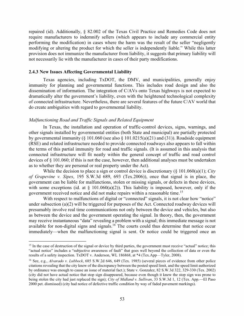
53

repaired (id). Additionally, § 82.002 of the Texas Civil Practice and Remedies Code does not require manufacturers to indemnify sellers (which appears to include any commercial entity performing the modification) in cases where the harm was the result of the seller “negligently modifying or altering the product for which the seller is independently liable.” While this latter provision does not immunize the manufacturer from liability, it suggests that primary liability will not necessarily lie with the manufacturer in cases of their party modifications.

2.4.3 New Issues Affecting Governmental Liability

Texas agencies, including TxDOT, the DMV, and municipalities, generally enjoy immunity for planning and governmental functions. This includes road design and also the dissemination of information. The integration of C/AVs onto Texas highways is not expected to dramatically alter the government’s liability, even with the heightened technological complexity of connected infrastructure. Nevertheless, there are several features of the future C/AV world that do create ambiguities with regard to governmental liability.

Malfunctioning Road and Traffic Signals and Related Equipment

In Texas, the installation and operation of traffic-control devices, signs, warnings, and other signals installed by governmental entities (both State and municipal) are partially protected by governmental immunity (§ 101.060 (see also § 101.0215(a)(21) and (31)). Roadside equipment (RSE) and related infrastructure needed to provide connected roadways also appears to fall within the terms of this partial immunity for road and traffic signals. (It is assumed in this analysis that connected infrastructure will fit neatly within the general concept of traffic and road control devices of § 101.060; if this is not the case, however, then additional analyses must be undertaken as to whether they are personal or real property under the Act).

While the decision to place a sign or control device is discretionary (§ 101.060(a)(1); City of Grapevine v. Sipes, 195 S.W.3d 689, 693 (Tex.2006)), once that signal is in place, the government can be liable for malfunctions, stolen or missing signals, or defects in these devices, with some exceptions (id. at § 101.060(a)(2)). This liability is imposed, however, only if the government received notice and did not make repairs within a reasonable time.15

With respect to malfunctions of digital or “connected” signals, it is not clear how “notice” under subsection (a)(2) will be triggered for purposes of the Act. Connected roadway devices will presumably involve real time communications not only between the device and vehicles, but also as between the device and the government operating the signal. In theory, then, the government may receive instantaneous “data” revealing a problem with a signal; this immediate message is not available for non-digital signs and signals.16 The courts could thus determine that notice occur immediately—when the malfunctioning signal is sent. Or notice could be triggered once an

15 In the case of destruction of the signal or device by third parties, the government must receive “actual” notice; this “actual notice” includes a “subjective awareness of fault” that goes well beyond the collection of data or even the results of a safety inspection. TxDOT v. Anderson, WL 186868, at *4 (Tex.App—Tyler, 2008). 16 See, e.g., Alvarado v. Lubbock, 685 S.W.2d 646, 649 (Tex. 1985) (several pieces of evidence from other police citations revealing that the city knew of the discrepancy between the posted speed limit, and the speed limit authorized by ordinance was enough to cause an issue of material fact.); State v. Gonzalez, 82 S.W.3d 322, 329-330 (Tex. 2002) (city did not have actual notice that stop sign disappeared, because even though it knew the stop sign was prone to being stolen the city had just replaced the sign); City of Midland v. Sullivan, 33 S.W.3d 1, 12 (Tex. App.—El Paso 2000 pet. dismissed) (city had notice of defective traffic condition by way of faded pavement markings).

54

employee has reason to discover the defect from the incoming data. As a result of the future legal uncertainty, which presumably could discourage the government from utilizing connected or digital technologies for fear of greater liability, legislative clarification of the notice requirement would be beneficial.

It is also possible, however, that since connected infrastructure malfunctions occur with respect to the transmittal of “data or information,” the courts might exempt malfunctions in connected infrastructure from liability altogether. This exemption would occur if the digital infrastructure is categorized in this context as “data” devices rather than “personal” or “real property” (§ 101.021). (See, e.g., Univ. of Tex. Med. Branch v. York, 871 S.W.2d 175, 178-179 (Tex. 1994) (holding that information is an “abstract concept, lacking corporeal, physical or palpable qualities,” and thus intangible)).17

Roadway Maintenance

C/AVs may also present additional liability risks to TxDOT and municipalities with respect to their road maintenance responsibilities. Some of the ways that C/AVs could alter the current liability landscape include:

• Special defects on the roadways, such as excavations and roadway obstructions. These obstructions can lead to potential liability of governmental entities if these defects are not addressed in a reasonable way—e.g., with signage, fencing, etc. (§ 101.060(c)).18 The capabilities of C/AVs to detect these defects may differ from non-automated vehicles, leading to a different set of required signals for C/AVs. TxDOT and other governmental entities responsible for these special defects may need to develop best practices for meeting their obligation of reasonable care with respect to AVs that rely on sensors.

• Differing vulnerabilities with regard to road repair. C/AVs may have the capacity to learn of and avoid certain types of road defects, such as potholes, using digital information on landforms that far exceed the abilities of human drivers. Conversely, there are some roadway hazards that may stump C/AVs but are easy to avoid for human operators. Blowing debris (paper bags) or perhaps other visual obstructions that in fact are not real

17 See also:

• Univ. of Tex. Health Sci. Ctr. v. Dickerson, 2014 Tex. App. LEXIS 1889, *19 (Tex. App.—Houston [14th Dist.] 2014, no pet.) (“[T]he use of computers, telephones or records to collect and communicate information is not a use of tangible personal property under [the Tort Claims Act,]” and “cannot provide the basis for a waiver of immunity under the [Act].”)

• Dear v. City of Irving, 902 S.W.2d 731 (Tex. App.—Austin, 1995 writ denied) (“The Supreme Court has specifically held that the Tort Claims Act does not eliminate governmental immunity for injuries resulting from the misuse of information.”)

• Axtell v. Univ. of Tex. at Austin, 69 S.W.3d 261, 263 (Tex. App.—Austin, 2002 no pet.) (“The tangible personal property exception of the Act does not encompass an injury resulting from the disclosure of confidential information, however that information is transmitted.”)

18 “A special defect” under § 101.060(c) is “an excavation or roadway obstruction [that is a] present ‘[] unexpected and unusual danger to ordinary users of roadways.’” State v. Rodriguez, 985 S.W.2d 83, 85 (Tex. 1999). See also Morse v. State, 905 S.W.2d 470, 475 (Tex. App.—Beaumont 1995, writ denied) (holding that ten-inch drop-off along shoulder that prevented car's left wheels from reentering the roadway once they had slipped off was a special defect); see, e.g., State Dep't of Highways v. Kitchen, 867 S.W.2d 784, 786 (Tex. 1993) (holding that ice on bridge during winter was not a special defect because it is not unexpected or unusual).

55

impediments, for example, could lead to considerable delays and inconveniences for C/AVs but not for non-automated vehicles.

Cumulatively, TxDOT may face twice the maintenance burden, or at least a more extensive

maintenance challenge, in a world of mixed vehicles where hazards are perceived differently. Moreover, the standards for reasonableness may become more of a moving target, particularly for hazards that are unique to C/AVs.

2.4.4 Implications of Liability Challenges for Insurance

At least some insurance companies predict that the effects of C/AVs on their net payouts and profits may ultimately be a wash. Insureds who drive C/AVs may face fewer crashes, but the cost of this vehicle—when there is a crash—may offset the reduced crash rate since the vehicle’s replacement/repair value is likely to be greater than the cost of an average non-automated vehicle (Swiss Re Centre for Global Dialogue 2015; see also Glancy et al. 2015 p.65). At best, the insurance industry seems to believe that the financial gains from insuring C/AVs is currently uncertain (Insurance Information Institute 2015).

Insurance companies are also reportedly wary of the increased costs of crash litigation that are likely to arise as C/AVs become more integrated on roadways. As discussed above, these increased litigation costs result from novel product liability claims against the manufacturers that may become commonplace in crashes caused in part by a C/AV (id.). Insurance companies may seek to circumvent these transaction costs by altering the contractual arrangements or by devising other methods to limit the costs of crash litigation in the future (ITS International 2015).

Finally, insurance companies are likely to take advantage of the ability of C/AVs to store and share data (Scism 2013). “Because connected vehicles provide rich sources of information about both vehicles and drivers, automobile insurance companies have taken a [particularly] keen interest in connected vehicles and the data they generate” (Glancy 2014, p.1647). This data will not only be central in resolving responsibility in crashes, but may also be available to insurers in setting premiums for individual drivers.

2.5 Privacy and Security

One of the most significant policy challenges facing C/AVs is ensuring the appropriate level of privacy and security for consumers. The information-intensive feature of C/AVs raises unresolved issues of how much data will be collected and/or recorded within the vehicle, who will “own” or have access to the data, and the resulting implications for personal privacy of users (Anderson et al. 2014, p.94). At the same time and in contrast to tort liability, because privacy and security are relatively new social issues, there is not yet a coherent legal infrastructure in place to manage them. The combination of technological uncertainties and legal instability presents challenges that are particularly acute for states at the cutting edge of integrating this new technology.

This section provides a very brief summary of the factual backdrop and then considers how the privacy and security issues are being treated under current law in Texas and nationally.

56

2.5.1 Privacy Concerns

There is widespread consensus that C/AVs will pose threats to traditional understandings of individual privacy. While there are risks to the disclosure of personal identifying information, like a driver’s license, the bulk of concerns related to risks posed by having personal information collected and used—generally to the consumer’s detriment—by manufacturers, insurers, and others. A great deal of data on the location, movement, habits, and other features of drivers will become available in a connected system and will even be recorded and potentially accessed in C/AVs that are self-contained (Woodyard and O’Donnell 2013; Markus 2013; Glancy 2012). One set of authors conclude that “[e]ven if this data is scrubbed of unique individual identifying markers, for instance VIN-numbers, or IP- or MAC- addresses, data-mining techniques will almost certainly be able to reconstruct personal identifying information about particular vehicles and by extension their regulator occupants” (Kohler & Colbert-Taylor 2015, p.120-121).

CVs that rely on infrastructure or vehicle communications will present the greatest risk of loss of private information (Glancy 2014), particularly if they cannot be turned “off” by the user so that information continues to be shared with third parties. The operating mechanism of these vehicles is premised on sharing information with other vehicles and/infrastructure in a type of data cloud. Moreover, information on the movement and operation of vehicles, particularly in connected systems, may also need to be stored and analyzed to improve the system. “A new car may have more than 145 actuators and 75 sensors, which produce more than 25GB of data per hour. The data is analyzed by more than 70 onboard computers to ensure safe and comfortable travel” (Glaskin 2014, p.40). In one of the most rigorous analyses of privacy and security risks associated with connected systems, Prof. Glancy identifies at least five distinct features of CVs that present particular risks to privacy (p. 1635; and p.2639-40). Figure 2.4 illustrates the various data components in V2V technology.

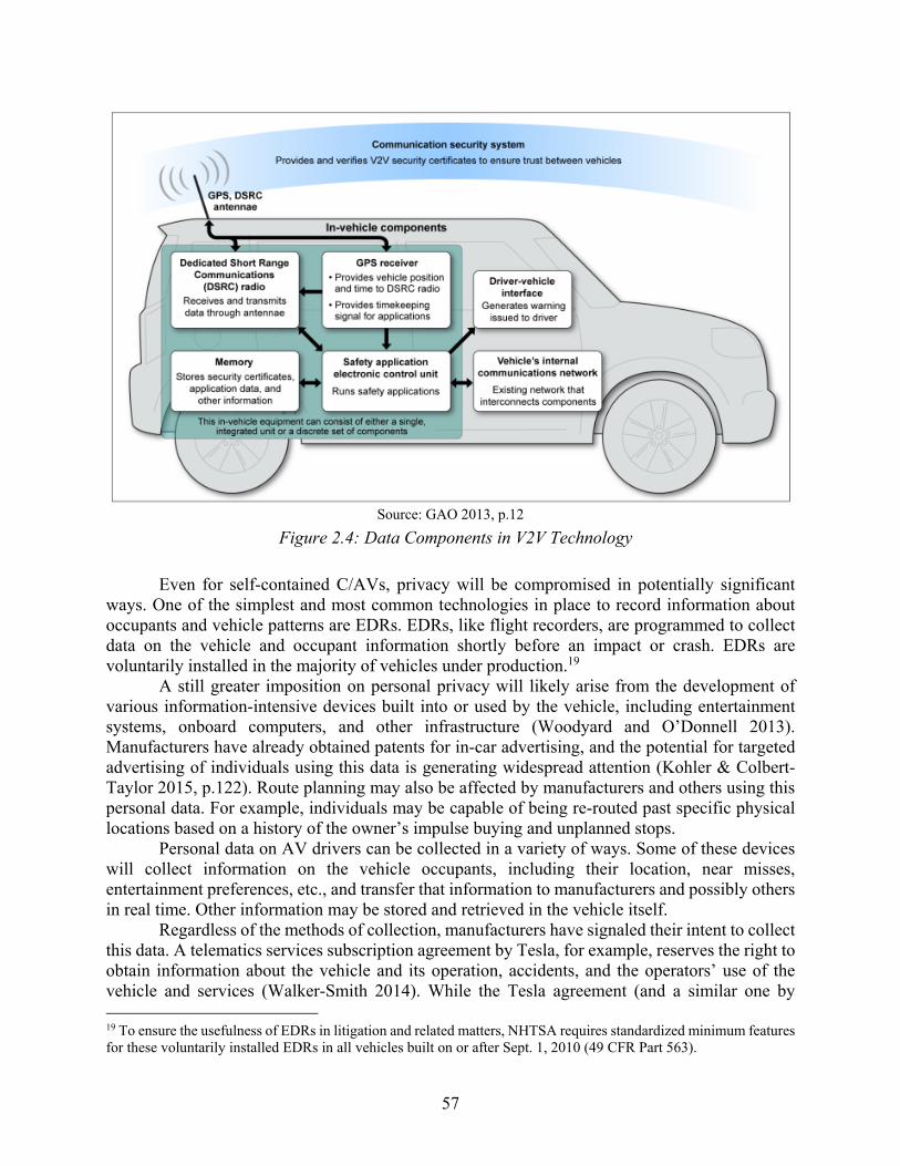
57

Source: GAO 2013, p.12

Figure 2.4: Data Components in V2V Technology

Even for self-contained C/AVs, privacy will be compromised in potentially significant ways. One of the simplest and most common technologies in place to record information about occupants and vehicle patterns are EDRs. EDRs, like flight recorders, are programmed to collect data on the vehicle and occupant information shortly before an impact or crash. EDRs are voluntarily installed in the majority of vehicles under production.19

A still greater imposition on personal privacy will likely arise from the development of various information-intensive devices built into or used by the vehicle, including entertainment systems, onboard computers, and other infrastructure (Woodyard and O’Donnell 2013). Manufacturers have already obtained patents for in-car advertising, and the potential for targeted advertising of individuals using this data is generating widespread attention (Kohler & Colbert-Taylor 2015, p.122). Route planning may also be affected by manufacturers and others using this personal data. For example, individuals may be capable of being re-routed past specific physical locations based on a history of the owner’s impulse buying and unplanned stops.

Personal data on AV drivers can be collected in a variety of ways. Some of these devices will collect information on the vehicle occupants, including their location, near misses, entertainment preferences, etc., and transfer that information to manufacturers and possibly others in real time. Other information may be stored and retrieved in the vehicle itself.

Regardless of the methods of collection, manufacturers have signaled their intent to collect this data. A telematics services subscription agreement by Tesla, for example, reserves the right to obtain information about the vehicle and its operation, accidents, and the operators’ use of the vehicle and services (Walker-Smith 2014). While the Tesla agreement (and a similar one by 19 To ensure the usefulness of EDRs in litigation and related matters, NHTSA requires standardized minimum features for these voluntarily installed EDRs in all vehicles built on or after Sept. 1, 2010 (49 CFR Part 563).

58

Nissan) makes clear that data will be collected, users may not fully appreciate the extent that their privacy might be compromised. The agreement allows the company to collect the following:

(x) information about the vehicle and its operation, including without limitation, vehicle identification number, location information, speed and distance information, battery use management information, battery charging history, battery deterioration information, electrical system functions, software version information, and other data to assist in identifying and analyzing the performance of your Tesla EV; (y) information about your use of the Services; and (z) data about accidents involving your Tesla EV (for example, the deployment of air bags) (Id. quoting Tesla agreement, at 1789).

Prof. Walker-Smith also notes that under the agreement,

the customer “owns” these data but “grant[s] to Tesla a worldwide, royalty free, fully paid, transferable, assignable, sublicensable (through multiple tiers), perpetual license to collect, analyze and use” them. These data may help the company to check, maintain, analyze the performance of, and help in the maintenance of the vehicle; “research, evaluate and improve” its technology; “comply with the law and any and all legal requirements,” including valid enforcement requests and orders; “protect the rights, property, or safety of” the company, the customer, or others; and “perform market research for Tesla’s own purposes,” a list that “is not meant to be exhaustive” (Id., at 1790, footnotes omitted).

Governmental entities can also collect personal information on operators driving on Texas highways, even without a connected infrastructure and V2I communications. In the State of Texas, for example, governmental entities have collected drivers’ information with Bluetooth readers and other easily available tools (Examiner 2015). But in the future, with V2V and V2I possibilities just on the horizon, the data will not only become more readily available, in some cases extensive data collection will be necessary to enable the connected infrastructure to direct traffic. While it is possible that the connectivity equipment can use the data only in real time, without storing it, this less intrusive option may prove inadequate for purposes of accident reports, technological capabilities, etc. Thus, TxDOT and other entities may find themselves faced with databases on consumer travel habits that contain some private information, regardless of their best efforts to avoid this scenario.

Alongside more immediate privacy concerns associated with data storage and use is the government’s own routing decisions that may be viewed as “infring[ing] on the individual right to privacy, including the right to physical autonomy” (Kohler & Colbert-Taylor 2015). The government could use routing to bypass protests or provide some drivers with more rapid routes than others. The latter possibility is particularly worrisome if faster routes are reserved for drivers with a higher status or a willingness to pay for the privilege.

The seemingly inevitable future for C/AV technologies is thus one in which the traditional concept of privacy and the infringement on individual autonomy by both the private and public sector will be more limited. Yet the point at which privacy and/or security interest are being breached or the appropriate state reaction to unrestricted consumer data collection, particularly by private businesses, is open to debate. The law governing this area, moreover, is still developing, offering little guidance in the interim.

59

2.5.2 The Law Addressing Privacy Concerns Involving C/AVs

Current Texas law unevenly places restrictions on the ability of governments or private entities to collect, tabulate, or even share (or sell) data on individual driving habits. Meanwhile, the collection and use of remaining information that nevertheless charts the location, use, accidents, etc., of a vehicle and its operator appears largely unprotected under Texas law.

Protection of Sensitive Information

The laws in the State of Texas provide citizens with strong protection from third-party access to sensitive information and information contained in EDRs. EDRs provide a particularly good reference point since much of the data collected in EDRs may not be terribly different from the types of data that can be collected through other devices installed in a C/AV as just discussed. In Texas, any governmental or private access to EDR data is generally off-limits except in one of the following four narrow categories:

(1) On court order; (2) With the consent of the owner for any purpose, including for the purpose

of diagnosing, servicing, or repairing the motor vehicle; (3) For the purpose of improving motor vehicle safety, including for medical

research on the human body’s reaction to motor vehicle accidents, if the identity of the owner or driver of the vehicle is not disclosed in connection with the retrieved information; or

(4) For the purpose of determining the need for or facilitating emergency medical response in the event of a motor vehicle accident. (§ 547.615(c))

These protections of privacy in Texas are reinforced by other laws that protect other

sensitive information. Under Texas Transportation Code §§ 371.001 & 371.051, license plate data collected on toll roads are not allowed to be collected or shared except for very limited official purposes. Motor vehicle records also cannot be subject to the State’s Open Records Act, thus providing some privacy protection for the release of driver’s license and registration information or other personal identification information (§ 552.130(a)). The federal Driver Privacy Protection Act reinforces Texas’s law. It prohibits state motor vehicle offices from disclosing photos, name, address, telephone number, and medical or disability information, with narrow exceptions (18 U.S.C. § 2721).20 Several federal statutes also protect consumer privacy in ways that would seem to at least preclude unauthorized interceptions of signals from C/AVs (Glancy et al. 2015, p.81-83).

Private businesses are also prohibited from allowing “sensitive personal information” of individuals to be accessed by third parties without consent of the owner (§ 521.052). “Sensitive information” for purposes of the Act includes specifically enumerated information that consists of medical information, Social Security or drivers’ license information, or credit card information. In cases of a breach or disclosure, the businesses are also required to notify individuals that their sensitive personal information has been accessed illegally (§ 521.053).

20 Note that the Act “prevents private actions against states.” Travis v. Reno, 163 F.3d 1000, 1006-1007 (7th Cir. 1998); Downing v. Globe Direct LLC, 806 F. Supp. 2d 461 (D. Mass. 2011), aff’d, 682 F.3d 18 (1st Cir. 2012) (“Congress, moreover, has not abrogated the States' sovereign immunity with respect to private DPPA lawsuits.”).

60

Limitations in Current Laws with Respect to Privacy and C/AVs

While it is conceivable that the data collected by manufacturers, the government, and others in a C/AV system would include some “sensitive” information under Texas law, personal information in the C/AV context likely includes a wealth of other personal information that does not fall into this “sensitive information” list but is nonetheless considered private (§ 521.002(2)). The statute does not appear to reach this information. Accordingly, if OEMs, software companies, or insurers install data chips, road cameras, or other mechanisms to collect information on individual drivers outside of the EDR, there appear to be no explicit legal prohibitions, restraints, or even requirements of disclosures for these various avenues of information access under Texas law. While consumers may have claims under contract law or tort law, even these prophylactic private remedies are likely to be incomplete at best.

Additionally, even with respect to “sensitive information,” there appears to be no prohibitions for private businesses in legal possession of the data to use it for internal commercial purposes (e.g., targeted marketing strategies); the law precludes “unlawful” use and “disclosure” to third parties, but it does not appear to prohibit commercial use of data for purposes of product development, advertising, or pricing and sales (§§ 521.051-.053 (in 521.051(a) consent appears required only when the sensitive information is used to acquire goods in the person’s name)). Federal legislation does not fill in these gaps in state protection (GAO 2012).

Insurance companies may also be able to gain access to this non-sensitive information under current law, perhaps through sales arrangements with the OEMs or others. Through a much more fine-grained understanding of the drivers’ habits (e.g., speeding, nighttime driving; handoffs; etc.), insurance companies can develop much more accurate policies governing insureds or avoid some drivers altogether. In fact, insurance companies are currently recruiting volunteer policy-holders to use devices to track their habits, thereby reducing their premiums (Glancy 2014; Scism 2013). While this activity is voluntary, it signals the insurers’ great interest and use for this personal information that falls outside of the narrower radius of “sensitive information.”

In contrast to private parties, the Fourth Amendment does impose constraints on governmental entities’ ability to collect private information on drivers (Glancy 2014). It is not clear at what point at which those protections might be triggered in cases where individualized personal data is collected or analyzed by the government beyond the infrastructure needs of V2I and V2V (Kohler & Colbert-Taylor 2015). It seems likely that the routine management and oversight of a C/AV system would not trigger these constitutional protections since they do not have surveillance or the “search” of individuals as their purpose and may not provide identifying information (Glancy 2014). Even in cases in which the data is used by the government in investigating the conduct of an individual driver, however, some have argued that the government may be allowed to access this data outside of the Fourth Amendment through a rigorous licensing program that provides the government with a type of implied consent to the information (Roseman 2014, p.32). The scope of the government’s access to the information, however, deserves considerably more analysis, which in turn will depend on a better understanding of the types of information and access that will be available in C/AVs in the future (Glancy 2014; Palodichuk 2015).

On the other hand, municipalities and state agencies—outside of constitutional violations—are immune from private tort claims from those whose information was shared, even in cases where sensitive information is disclosed in violation of Texas law. As discussed earlier, state agencies and municipalities may be immune from suit with respect to negligent acts that involve the disclosure of information, including presumably confidential information. In the State

61

of Texas, as contrasted with several other states, there also appear to be no requirements that the State notify persons if or when their data has been breached, even as a result of the State’s negligence (Froomkin 2009).

Texas law not only immunizes the government, but it may actively require agencies to disclose all unprotected information, even if it identifies citizens, through the Open Records Act. Protected information includes that information expressly prohibited from disclosure under § 552.130(a) and federal law; only “information considered to be confidential by law, either constitutional, statutory, or by judicial decision” is exempt from disclosure (§ 552.101). Thus, to the extent that the State collects, processes, stores, or otherwise is in possession of additional information on individual vehicles (e.g., make, model, speed, location and time), it may be required to share this information upon request.21

Legal Developments outside of Texas

There is proposed legislation at the federal level that specifically addresses the risks to consumer privacy as a result of the new C/AVs technology. In July 2015, Senator Markey introduced the “Spy Car Act of 2015” (S. 1802). (The bill follows President Obama’s broader call for a “Consumer Privacy Bill of Rights” in 2012, which attempts to provide protections for consumer privacy across a broad range of areas; see Kohler & Colbert-Taylor 2015). Senator Markey’s bill did not make it through committee, but the bill signals congressional interest in addressing the privacy (and hacking) issues associated with C/AVs (U.S. Congress 2015). The proposed law would, among other things, direct NHTSA to promulgate a rule that protects against unauthorized access to information regarding the owner, speed of the vehicle, data stored in the car, etc., and also requires cars manufactured with accessible data to be capable of reporting and intercepting unauthorized access. The bill also directs NHTSA to conduct a rulemaking to require a “cyber dashboard” to inform consumers about the extent of protection of their privacy beyond a narrow set of sensitive data. Finally, the bill directs the FTC to conduct a rulemaking that would require that purchasers be notified of data access and collection on their activities; to provide them the option to decline this collection and retention (except for critical safety and post-accident information); and to prohibit manufacturers from using the collected information without the consent of the owner or lessee.

At the regulatory level, both NHTSA and the FTC have taken a focused interest in restricting hacking and intrusions on the privacy of consumer data in C/AVs (Glancy 2014; Kohler & Colbert-Taylor 2015). The FTC, for example, already engages in some oversight of this new market through its regulation of unfair or deceptive trade practices, which could include unjustified invasions of consumer privacy (Glancy 2014). The National Institute of Standards and Technology has also developed best practice standards to manage cybersecurity vulnerability which provide at least some initial protection against the worst security breaches.

At the state level, at this point only one state appears to have passed a law to address the consumer privacy related to C/AVs—the State of California. California requires that a “manufacturer of the autonomous technology installed on a vehicle shall provide a written disclosure to the purchaser of an AV that describes what information is collected by an autonomous technology equipped on the vehicle” (Chapter 570, DIVISION 16.6. § 38750(h)). Since the law is

21 The courts impose privacy exceptions in some cases, for example, if the information sought to be disclosed is highly embarrassing and has no public value. See, e.g., Indus. Found. of S. v. Tex. Indus. Accident Bd., 540 S.W.2d 668, 685 (Tex. 1976).

62

only 3 years old, it is too early to predict its implications for manufacturers of C/AVs sold in the State or even sold outside the state. The California law has also been criticized by consumer groups as taking too soft a stance on the ability of OEMs and others to collect private information (Lenth 2013, p.796).

Finally, with respect to government-related disclosures or breaches of confidential information with respect to its citizens, roughly half the States require by legislation that a governmental entity notify persons of the breach of confidentiality in cases where the government was the cause of the breach (Froomkin 2009). Out of these states, only a few allow suit to be brought by an individual against the state if it does not report the breach in a timely manner. In Louisiana, for example, the fine is not to exceed $5,000 for each violation, while in New Hampshire the plaintiff receives such damages as “the court deems necessary and proper.” Agencies in states that do not allow individuals to bring suit can still face fines or suits from the state’s Attorney General or other centralized authority.

In these various laws, there appear to be two general approaches to the privacy challenges arising with respect to C/AVs. One approach limits or even prohibits the use of certain technological mechanisms for data collection. The second approach requires manufacturers and software developers to disclose the nature of the information they can gather on consumers in an accessible way. Despite their different institutional mechanisms of oversight, running through both approaches is the premise that without some early legal oversight of the privacy-related features of the technology, the “genie will be out of the bottle.” OEMs, software developers, and perhaps even insurers that become accustomed to and develop financial plans premised on access to private data will both resist and face high costs in altering their plans if that easy data access is constrained later, down the road.

2.5.3 Security Concerns and the Existing Law

A related but very different risk from the data-intensive operations of C/AVs is the potential for security breaches that endanger life as well as financial and other private information through criminal hacking of the data and infrastructure. Some of the more frightening scenarios include a terrorist who is able to hack into a CV system and direct all cars to drive off bridges into the water or crash into one another (Douma and Palodichuck 2012).

Engineers and others familiar with the technological systems concede that the hacking risks are not trivial and that C/AV systems cannot be designed in ways that are completely free of hacking risks. Stop buttons may have the potential to electronically disengage vehicles, allowing some operator control over the worst types of data-hacking. Yet short of this ability to stop some terrorist manipulation of complete transportation systems, the other types of risks of hacking into data systems remain a continuing concern.

Another set of scenarios involve using self-driving cars remotely as bomb-depositors or drug-traffickers. In this security breach, the larger system is not hacked (Douma and Palodichuck 2012); rather, a single car itself or series of cars are remotely controlled for criminal purposes. Since anonymity is difficult to achieve, criminal commentators are more sanguine about the ability of the criminal system to sanction these types of uses (id). Still, the remote use of C/AVs provides a new tool in the arsenal for mass attacks that will need to be factored into the larger criminal justice equation.

While not specifically tailored to the hacking of C/AVs, there are several federal laws that appear to penalize these attempts, including the Computer Fraud and Abuse Act, the Digital Millennium Copyright Act, the Wiretap Act, and the USA Patriot Act (Kohler & Colbert-Taylor

63

2015). Texas Penal Code (Title 7, Chapter 33) also provides anticipatory deterrence against hacking. “A person commits an offense if the person knowingly accesses a computer, computer network, or computer system without the effective consent of the owner” (Tex. Penal Code Ann. § 33.02(a)). The penalty is dependent upon the aggregate amount of money involved (id. at § 33.02(b-2)). The aggregate amount consists of the “benefits obtained and the losses incurred because of the fraud, harm, or alteration” (id. at § 33.02(c)). A violation of this statute ranges from a Class B misdemeanor to a felony of the first degree (id. at § 33.02(b-2)). If the hacker obtains the identifying information of another, the violation is upgraded to either a second degree or first degree felony regardless of the amount in question (id).

2.6 Conclusions and Recommendations

There are numerous public and private benefits associated with C/AVs, but these technologies also present risks and challenges to our transportation systems. In this chapter we investigated the legal status and near-term legal issues associated with the liability, licensing, and privacy of C/AVs in the State of Texas. Although this reconnaissance work considers the law from numerous vantage points, we are particularly attentive to how the introduction of C/AVs in the State may affect the priorities, liability, and responsibilities of TxDOT.

This bird’s eye view of the intersection of the law and the use of C/AVs in Texas reveals several areas that deserve legislative and regulatory attention (as well as additional research) in the near term. First and perhaps most immediate is the need for policymakers to consider whether the testing and deployment of C/AVs in the State will benefit from more formal, legal oversight. A second, near-term issue at the intersection of C/AVs and Texas law is the need for some adjustments to current liability laws, including with regard to TxDOT’s responsibilities, in order to provide greater predictability as these new vehicles are tested and deployed on Texas roadways. Finally, C/AVs present a number of important public conflicts arising at the intersection of driver privacy, autonomy, and security. While NHTSA and the FTC appear to be taking primary responsibility for the development of national standards and directives, several State-specific reforms may also be beneficial to minimize the risks of C/AVs to the privacy and autonomy of Texas citizens.

A number of other, less immediate legislative guidelines identified in this chapter should further streamline the integration of C/AVs, providing both predictability to the industry and raising the trust and safety of the vehicles as they become prevalent on Texas highways. By identifying the “low-hanging-fruit” in need of some attention within the State, the chapter identifies a number of issues that are not only well-positioned for State legislative guidance, but for which the lack of legal action itself constitutes a choice.

2.6.1 The Need for Immediate and Long-term Planning

The transition from HVs to CAVs will not just bring benefits to the state of Texas but also present challenges that will need to be addressed. Several U.S. states have already taken steps in preparing for this paradigm change, and Texas will need to do the same. Listed below are strategies that the project team feel are of importance to ushering in CAV use, organized into three flexible time periods: short term (next 5 years), medium term (5–15 years), and long term (15+ years). The associated descriptions should begin a discussion of the steps that Texas can take to best prepare the state transportation system for the onset of CAVs.

64

Today’s vehicles operate under human control, relying on human senses and reflexes. Level 2 CAV technologies are being installed in both the vehicles themselves and within the transportation infrastructure that seek to augment human senses and reflexes for enhancing safe operations. Level 4 vehicles are building on the current work, with the likelihood of extensive street and highway operations within 5 years. There are challenging legal liability issues arising in these developments for FHWA and the state DOTs, state Departments of Motor Vehicles and local governments. One of the most important of these issues will be at the interface of these agencies as C/AV Standard Setting Organizations (SSOs) and the bounds of their sovereign immunity.

A near term example can be found in the lane markings—paint stripes and road “buttons”—whose standards are incorporated in the Manual of Uniform Traffic Control Devices (MUTCD). A number of different trials have shown that certain conditions (rain, snow, etc.) seriously degrade C/AV sensors’ ability to correctly recognize lane markings. Work is already underway at the Texas A&M Transportation Institute to determine standards that seek to increase correct identification by the various sensor types available for C/AVs. DOT or municipal transportation departments must show that they regularly maintain the effectiveness of lane markings to avoid liability. It will take some years in actual use to determine the length of time the new C/AV compatible lane markings remain effective, allowing public agencies to set up defensible maintenance schedules.

Mid-term examples will be the RSE devices and other transportation system infrastructure whose technical standards and operations/maintenance standards are currently in development. These technologies are essentially wholly new in highway transportation operations. The RSE that identifies a wrong-way driver must tie in to warning devices in suitably equipped C/AVs as well as provide an appropriate warning to “dumb” vehicles. And, in addition to the vagaries of weather and any limits imposed by basic design, the RSEs will need to be secure against cyber-attack and unintended cyber interference. Whatever standards are set must stand up to liability claims based on possible public agency failures in designing or maintaining them with due technical and practical diligence.

In the long term, the standards set by the public transportation agencies for C/AV operations will be focused on maintaining adequate levels of transportation capacity and minimizing congestion. TxDOT will be inextricably linked into the process and infrastructure for using “platooning,” continuous flow intersections, and other traffic management systematic approaches for increasing roadway capacity safely. Continuous flow intersections in “urban canyons,” for instance, will undoubtedly need extremely accurate survey “benchmarks” and cyber protected operations algorithms to be effective and safe. In these circumstances, it is likely that TxDOT will need to completely redo its design, operation and maintenance manuals to reflect the complete change in system dynamics driven by C/AV technology. And, again, all these changes and additions will need to be demonstrably appropriate and diligent, with continuing likelihood of maintaining suitable and safe operations.

TxDOT should (a) advise the Commission and the Legislature on these liability impacts; (b) coordinate with other state and AASHTO stakeholders in C/AV related standards development; and (c) when appropriate, recommend changes in the TTC and TAC aimed at minimizing liability in times of fast technological change.

2.6.2 Getting from Here to There

In short, although the future is uncertain with regard to how C/AVs will assimilate into the existing Texas transportation system, there appears to be little doubt that some assimilation will

65

occur over the next few decades. The literature suggests that policymakers will follow one of two general paths: 1) legislators will pass a holistic program to guide assimilation of the new technology into the state (for examples of this, see Appendix G); or 2) policymakers will develop incremental regulations or legislation to address specific impediments or public concerns as they arise (OECD 2015).

The choice between a holistic or incremental approach, however, takes the policymaker only so far; he or she still must select the topics, issues, and alternatives that deserve legal attention. In the recommendation section offered here, we present the options as a smorgasbord or matrix of possibilities organized by policy topic. The matrix in Table 2.4 provides a mix-match set of options and issues, leaving it to policymakers to determine the approach, as well as the priorities and preferences, with regard to pursuing each and every issue. To provide some ease of use, the issues of concern within each column are ordered roughly by their immediacy. Presumably passing legislation to allow for vehicles without a human operator present is of lower priority than ensuring the legality of truck platoons. Also included in the menu are issues that do not yet appear ready for legal action, but nevertheless warrant attention (indicated with italics); for example, TxDOT or the Texas Legislature could request and develop focused information-collection and periodic reports to stay abreast of these potential issues that will benefit from legal attention down the line.

All of the items in Table 2.4 deserve careful consideration as State policymakers build a legal regime to facilitate the integration of C/AVs in Texas. The items in the shaded cells, however, are those that are likely to be of particular interest to TxDOT. Even for shaded items that ultimately require legislative attention, TxDOT seems to be the best entity to frame and engage the legislature in addressing the issues.

66

Table 2.4: Matrix of Topic Areas for C/AV Policies in Texas

Safety on the Highway: Section 2.3

Legality: Section 2.3

Liability: Section 2.4

State Responsibilities/Liability: Section 2.4

Privacy and Security: Section 2.5

Advance Broader Public Goals in C/AV Innovation: Section 2.6

Testing and development

Clarify the identity of ‘Operator’

Streamline simple crash claims;

Clarify what constitutes ‘notice’ for malfunction in digital traffic

Improve consumer information

Collect reports/information on C/AV

Vehicle registration/ certification

Clarify whether operator needs to be on board

Address other difficult liability issues

Exempt license plates and other identifiable information from disclosure under the State Open Records Act

Restrict the sharing or sale of consumer information in C/AVs to third parties

Encourage greater innovation on wide-ranging public benefit

Added operator requirements

Adjustments for truck platoons

Require State Agencies to alert individuals when their privacy is breached

Criminalize hacking

License plate tags or other markers

Legalize texting and other bad behavior

Encourage innovation in cyber security

Rules for intensive uses (e.g., truck platoons)

Before describing the various options and issues, it is important to note that another

plausible legal alternative, albeit one that entails greater public risk, is for Texas policymakers to take little to no legal action at all. As discussed in the analysis above, liability rules and even most of the licensing and rules of the road requirements will allow for the legal integration of C/AVs onto state highways without added legislation. While this “no action” alternative is not recommended by either NHTSA, the ULC Subcommittee, or in the considerable body of scholarly commentary (particularly regarding the testing and operation of C/AVs), it remains a legally plausible option for the State of Texas.

We first list a series of adjustments that are recommended to existing laws and programs, and then offer more targeted suggestions for TxDOT’s oversight of C/AVs.

2.6.3 Ensuring the Safety of C/AV Testing and Deployment on Public Highways

Although C/AVs promise to provide heightened safety, the newness of the technology, combined with some public concern, has prompted several states to engage in the oversight of basic safety features of the emerging technology as it enters public roadways. At the same time that there is pressure on state policymakers to provide some modicum of legal oversight on the use of C/AVs; both NHTSA and European leaders are cautioning against too much state intervention for fear it will chill the technology.

67

The consensus emerging from commentators is that states still play an important role in overseeing the testing and use of C/AVs driven within their states (ULC 2014). States are cautioned to resist the temptation to prescribe acceptable types of technology or impose requirements on vehicle manufacture and design; instead they play the leading role in overseeing the early use of the technology to prevent accidents on public highways. In the recommendations below, primary emphasis is thus placed on locating some least common denominator solutions—where the state can provide the greatest safety oversight with the least imposition on the development of this new technology.

Testing and Deployment of C/AVs on Texas Highways

[This recommendation may be of particular interest to TxDOT.] As discussed, because of the risk of accidents early in the use of the technology, coupled

with public concern about the new technology, there is a growing consensus that states should actively regulate the use of C/AVs at both the testing and the full deployment stage. Specifically, the ULC Subcommittee recommends a uniform state act that “expressly prohibit[s] any use (including testing) of autonomous vehicles on public roads except as expressly permitted by the uniform act” (ULC 2014, p.5). NHTSA also recommends specific assurances from persons seeking to test vehicles before allowing that testing (such as a demonstration of the technology in the past and a plan for minimizing risks during testing) (NHTSA 2013, p.11).

Several states have required agency approval for testing and deployment of C/AVs. In order to test a C/AV in Nevada, for example, the state requires added insurance; proof that one or more of the vehicles has been driven a combined minimum of 10,000 miles in autonomous mode; a demonstration of the technology to the DMV; and a demonstration that its technology can be driven in the geographic locations designated for testing (Nev. Reg. § 8.3). California requires identifying information to be provided to the DMV for each vehicle that is being tested (Cal. Regs. §227.16). Both Nevada and California require a license or permit for testing as well (Cal. Regs. § 227.04(d) and Nev. Regs. § 8.3).

By contrast, Texas currently has not passed laws or regulations to formally oversee the testing or deployment of C/AVs. As discussed, under current law C/AVs appear to be legal on Texas highways, at least if an operator is present. As a result, driverless vehicles with operators aboard may enter the public highways without notification to TxDOT or the Texas DMV, and without added government regulation or mandated reporting of their crashes or activities.

One option available to Texas is to prohibit the use of C/AVs for testing or deployment without prior authorization from TxDOT. Excellent recommendations based on past experience and state approaches are provided in Appendix G (see particularly UWash Tech [undated]). Because of the changes that are likely over the next decade or so in use of C/AVs, the Legislature may also wish to place a 10-year sunset on the law.

If Texas chooses to engage in formal oversight of the testing and deployment of C/AVs, it will need to define what a C/AV is, identify the nature of the oversight for testing, and may need to identify the point at which a “tested” vehicle is authorized for full deployment and/or restricted deployment on Texas roads. In regulating the testing of C/AVs in particular, the State could require (among various possibilities arising in the states) that tested vehicles have operators aboard during all testing; require some driver qualifications for AV operation; require insurance; limit testing with respect to certain areas; provide reports of crashes and near misses; and require crash data records be deployed and shared with the State. As a less onerous approach, the Legislature (or

68

perhaps even TxDOT) would require all testing to be reported to the State before it is conducted.22 This will allow the State to at least monitor the testing activity.

The more difficult decision in such an oversight law is identifying the appropriate point at which AVs pass “testing” and can be deployed on public highways. Several states (such as Nevada and California) require the statewide certification and approval of C/AV models before they can be driven on public roadways. An alternate approach is to require a minimum of test miles on public roads free of concerning accidents, with reporting of all driving tests to the State. The State might even allow use of C/AVs provided they meet one of several requirements that include not only some testing but take full legal responsibility for any crashes occurring in the state (Risen 2015).

As noted below, if testing involves the operation of cars without operators present in the vehicle, this testing would likely be in violation of § 545.404. If the State wishes to encourage the testing of C/AVs on Texas roadways without an operator aboard the vehicle, it will need to exempt testing of unoccupied, driverless vehicles from § 545.404 and may need to institute other controls to ensure safe testing conditions. Such added testing requirements could be included in a testing/oversight law.

Vehicle Registration of C/AVs

Under existing Texas law, C/AVs appear to be legal as long as the vehicle is registered and a licensed operator is present. The DMV safety inspection required for vehicle registrations does not appear to take into account the possibility that a vehicle has automated features.

The State of Texas could add additional safety requirements for C/AVs at the registration stage to ensure they meet minimum requirements. There are several safety features that both the ULC Subcommittee and NHTSA, as well as some states, believe are essential for a C/AV either tested or in use in the State:

1. Device to disengage the automated system. (See ULC 2014, p.9, for specifics on the varying requirements.)

2. Device to indicate whether the vehicle is operating in autonomous mode (p.10).

3. System to warn operator of failure.

For C/AVs, annual checks or on-line certifications of regular updating of the vehicle may also be valuable. Particularly in the early stages of automation, it is likely that the software and recall of vehicles may be an active area (OECD 2015, p.29). Owners will need to take responsibility for ensuring this is completed. Texas may insist on evidence that owners are fulfilling these responsibilities on an annual basis.

If the State chooses not to restrict or oversee the deployment of C/AVs on public highways, it also could use the vehicle registration requirement as a way to at least develop a reporting system for the number and types of C/AVs in use on highways. C/AVs might also be assigned special numbers or designations on the license plates, see Section 6.2.4.

22 States like Florida take an even more limited approach. Florida sets standards and require registration of C/AVs, but then allow them on roadways once registered. (To date, no applications for registration of AVs have been submitted). While this light-handed approach does not appear to be endorsed by model state law committees or academic commentators (see in particular UWash Tech, undated, in App. G), Florida’s approach offers yet another option for C/AV oversight that focusses on standards rather that state oversight during testing and deployment.

69

Added Operator Requirements

Under Texas law, there are also no additional licensing requirements imposed on operators of AVs. Some states require added endorsements or training for those wishing to operate an AV (ULC 2014, p.12). The State of California requires that the driver has undergone training by the manufacturer (Cal Regs. § 227.20). Restrictions on C/AV operators could also be instituted in Texas.

License Plate Tags or Other Indicators of C/AVs

Several states have enacted, and the ULC recommends, some public marker for C/AVs, such as a special license plate (ULC 2014, p.11). This recommendation may be particularly well-placed for the operation of truck platoons on highways. Since the requirement is imposed on owners and occurs during the licensing of the vehicle, this type of requirement would seem to have little to no negative impact on technological innovation or sales of C/AVs. Indeed, these demarcations could serve as a way to build public confidence and trust and may even boost the market for C/AVs as they become more commonplace.

Targeted Requirements for Intensive Uses of C/AVs like Truck Platoons

[This recommendation may be of particular interest to TxDOT.] Even without statewide legislation that restricts and regulates the use of C/AVs on Texas

roadways, some more intensive uses of C/AVs will require greater governmental oversight. Truck platoons are a particularly discrete type of C/AV that demands added government oversight during both testing and operation. Among the many regulatory decisions to be made are the following:

• whether to identify a designated lane and/or roadways pre-approved by TxDOT; platoons could be prohibited on other public highways in the State without advanced permission;

• size and length requirements, presumably promulgated by TxDOT, that restrict platoon length and the maximum number of units per platoons;

• a cap on the number of platoons allowed on a public road at any given time;

• passing requirements and restrictions;

• time of day rules, minimum speeds, and similar operational requirements.

The more intensive the use of highways by truck platoons, the more necessary it will be for TxDOT to revisit its pavement and bridge design standards. In revising these large-scale road features, there will need to be close interaction between TxDOT, the legislature, DMV, Department of Public Safety, and local jurisdictions along platoon routes. Finally, platoons will need to assemble/disassemble (or form and dissolve as directed while en-route to their destination), and the locations for this work ideally should be designated in advance, in locations that are appropriate, safe, and in keeping with the planning done by local governments.

State agencies like TxDOT are well-positioned to anticipate these and other challenges that arise from the use of truck platoons, but many of these challenges fall outside the four corners of the current legal and transportation system and thus require future legal directives. With respect to resources at least, Congress appears aware of some of these future challenges. Federal funding may be available in the future to support some of this work by TxDOT and other state agencies

70

(e.g., S. 1647, 114th Cong., 1st Sess. 2015—not passed by proposing targeted funding for smart transportation).

Legality

Regardless of whether the State regulates testing and deployment of C/AVs on Texas highways, some legal clarifications will be helpful in providing greater predictability for the legal requirements governing C/AVs. Indeed, these clarifications are more important if the State decides not to restrict the use of C/AVs.

Clarifying the Identification of an Operator

[This recommendation may be of particular interest to TxDOT.] As discussed in Section 2.1, the Texas Motor Vehicle Code places responsibility for

complying with all licensing requirements and traffic requirements on the “operator” of a vehicle. While “operator” is a broad term that appears to encompass sleeping occupants, there is nevertheless the possibility that the Code could be interpreted to allow (because it does not prohibit) the use of vehicles that are “operator-less.” Unlike vehicles with operators, moreover, these vehicles without occupants and without designated operators would be free of most of the licensing and rules of the road requirements since the Transportation Code places responsibility for compliance on the “operator” of the vehicle (rather than the vehicle itself).

In the short term, to avoid confusion, the State could clarify that each vehicle on the Texas highway must be controlled by a designated “operator” that meets the requirements of § 521.021 (“A person…may not operate a motor vehicle on a highway in this state unless the person holds a drivers’ license issued under this chapter”).

Clarifying whether Operators Must Be Aboard a Moving Vehicle

[This recommendation may be of particular interest to TxDOT.] The Texas legislature should also clarify whether an operator must be aboard a vehicle

during its operation since current law is ambiguous on that point. (Note that for at least testing, NHTSA “strongly recommends” that “states require that a properly licensed driver be seated in the driver’s seat and ready to take control of the vehicle while the vehicle is operating self-driving mode” (NHTSA 2013, p.12)). Section 545.404 does prohibit operators from leaving vehicles “unattended,” and the best reading of this Section is that the legislature intended to preclude the operation of vehicles without a human operator aboard the vehicle. Yet because of residual ambiguity, perhaps “unattended” could be amended to explicitly prohibit vehicles that are being remotely controlled.

Alternatively, if it is the case that Texas wishes to allow vehicles on public highways that do not have operators present, then the law should be amended to legalize these operator-less vehicles. Presumably, some safety requirements and limitations will also need to be included in this exception.

Legal Clarifications to Permit Truck Platoons

[This recommendation may be of particular interest to TxDOT.] If the State of Texas determines that truck platoons are a beneficial activity, then several

relatively minor adjustments to existing law will be needed to streamline their operations in the

71

Texas. As mentioned earlier, there are several rules of the road and motor vehicle requirements that conflict with the use of truck platoons (e.g., following distance; licensed operator in vehicle). Most of these conflicts could be cured by a regulatory determination that truck platoons are the legal equivalent of a single “tow” trucks for purposes of the law. Such an interpretation then allows for a closer following distance and operation without an operator.

Yet identifying truck platoons as “tow trucks” under the law still may be considered insufficient to ensure that this new technology is monitored and operating safely on Texas highways, at least during its first few years of introduction. For example, TxDOT or some other entity will also need to identify the appropriate lanes and routes for platoons, which in turn could require adjustments to the “no trucks in left passing lane” ban in place in some areas. Some accommodation may also be needed for merging on and off highways and for fueling and other necessities. Finally, legal clarification is needed to allow the “towing” of trucks in platoons to include multiple vehicles.

Thus, in terms of legal and policy attention, truck platoons seem to demand focused legislation or regulatory oversight. TxDOT or another agency should engage in this oversight or work with the legislature to ensure the proper requirements and preparations are in place to ensure a smooth integration of truck platoons onto State highways.

Legalize Texting and Other “Bad” Behaviors in Some Driving Settings

If driverless vehicles are deployed in ways that are believed by policymakers to be safe, then Texas may reward owners of these vehicles by lifting certain prohibitions for operators while driving in automated mode (OECD 2015 p.29). Texting while driving is illegal in some localities in Texas (TxDOT, Cell Phone Ordinances, undated).

If texting bans become more prevalent, the State could allow texting in identified driverless vehicles while in automated mode. Florida and Michigan have already passed laws permitting texting while operating an AV in autonomous mode (Fla. Stat. § 316.305(b)7, Mich Comp. Laws § 257.602b(4)(e); see also ULC 2014, p.13 with similar recommendations).

Other “bad” habits may also be exempted from civil and criminal liability in the State in narrowly tailored settings. For example, if driverless vehicles are able to operate safely without a competent operator, perhaps even alcohol consumption (including in the vehicle) might be allowed (see §§ 49.031, 49.04 for current prohibitions).

Adjustments to Tort and Private Injury Law

The strong consensus among commentators is that tort liability laws should be left undisturbed to the extent possible to allow the flexibility of the common law to adapt to the technological changes presented by C/AVs (UWash Tech, undated, p.20). Nevertheless, there are several modest adjustments that may deserve consideration to alleviate some of the most substantial concerns about the integration of C/AVs into existing tort liability law.

Streamlining Simple Crash Claims in C/AV Litigation

As C/AVs become more commonplace on highways and are implicated as the cause of crashes, what used to be “simple” crash litigation will necessarily include more complicated product liability claims against manufacturers. There are several approaches that could anticipate and alleviate some of this potential future uncertainty. The approaches could be used in all crashes

72

or only crashes that involve a limited amount of damage (perhaps less than $75,000), since it is the smaller cases that will be most impacted by these more complicated and expensive claims.

First, in deciding cases that involve allegations that the automated features of the vehicle in part caused the crash (thereby implicating the vehicle manufacturer), the Texas courts deciding common law claims could impose a non-delegable duty on the owner/operator consistent with the insurance coverage. Non-delegable duties can be imposed under the common law by courts deciding tort cases.23 With a non-delegable duty, the owner/operator would be the presumptive responsible parties. While the owner/operator of the AV could engage the vehicle manufacturer and others in a third-party suit for indemnification, a case brought by an outside party could recover all damages against only the owner/operator. If greater legal certainty is desired, the Texas legislature could also codify this type of legal responsibility on owners. The overriding goal of this legislative directive is to save accident victims, including TxDOT, from the expense and delay associated with unraveling responsibility among the manufacturer, driver, owner, and software developer, as well as others.

Alternatively, with respect to claims by third party victims harmed by a C/AV in automated mode (or perhaps all persons, including owners), the legislature could place the burden of proof on the manufacturer of the C/AV to establish that the crash was not caused by a defect in the vehicle. (There is some indication that the OEMs themselves may already be accepting this responsibility, although it is not clear if these commitments are legally binding [Volvo Car Group 2015]). For example, the law could direct that in crashes involving C/AVs as a possible cause, the OEM will be considered jointly responsible with the operator unless the OEM can establish that there was no defect in the vehicle, consistent with the rules of fault and product liability in the State of Texas.24 Given the loss-spreading and low crash rate of C/AVs, placing this responsibility on the manufacturers may be beneficial not only in streamlining liability but could even create greater trust in the market. Owners will appreciate the implicit “guarantee” that crashes will be rare and will have incentives to use the automation; manufacturers will have incentives to reduce crashes (see also Glancy et al. 2015, p.73-74). If a licensing and certification program is in place in the State, the placement of responsibility on manufacturers should also require that the C/AV at the time of the accident was properly licensed and legally permitted.

Although it is much more broad-reaching, the State could adopt a no-fault approach to liability for all cars or perhaps for C/AVs exclusively. It could also require alternative dispute resolution or other transaction-cost saving mechanisms for resolving responsibilities of actors involved in crashes that include at least one C/AV operating in autonomous mode. For more

23 See Maloney v. Rath, 445 P.2d 513, 516 (Cal. 1968) (providing examples of non-delegable duties in common law: “the duty of a condemning agent to protect a severed parcel from damage…the duty of landowners to maintain their property in a reasonably safe condition…to comply with applicable safety ordinances…the duty of employers and suppliers to comply with the safety provisions of the Labor Code….”). A non-delegable duty could be placed on C/AV operators for the for the criminal misuse of their vehicle, for example, federal courts have placed non-delegable duties on the purchasers of guns for their criminal misuse. See, e.g., City of Phila. v. Beretta U.S.A. Corp., 277 F.3d 415, 426 (3d Cir. 2002) (“Accordingly, we will dismiss plaintiffs' claims that tort liability should be assessed against gun manufacturers when their legally sold, non-defective products are criminally used to injure others.”). See First Commercial Tr. Co. v. Lorcin Eng'g, 900 S.W.2d 202, 205 (Ark. 1995) (holding that a firearm manufacturer is not responsible for the criminal misuse of its product); see also Riordan v. Int’l Armament Corp., 477 N.E.2d 1293, 1295 (Ill. App. 1985) (“[T]he distribution of handguns by the defendants-manufacturers was intended for the general public, who presumably can recognize the dangerous consequences in the use of handguns and can assume responsibility for their actions.”). 24 Strict liability on C/AVs manufacturers, as suggested by some commentators (Vladeck, 2014) is another option.

73

information on the pros and cons of these more systematic changes to the Texas liability rules, readers are referred to Anderson et al. (2014) and Funkhouser (2013).

The goal of these streamlining devices is to counteract the increased costs of litigation, particularly with respect to smaller scale crashes, associated with C/AVs. Without some type of anticipatory legislation, crash litigation will become more expensive, particularly for the victims harmed by C/AVs.

Several Other Difficult Liability Issues May Benefit from Legislative Attention

The ULC Subcommittee suggests that states may need legislation to address issues associated with consumer-imposed modifications to vehicles after-market (ULC 2014, p.5). Several states have already legislated immunity for manufacturers in cases where a third party modifies a C/AV and those changes, rather than a defect initially present in the vehicle, cause harm (Nev. Rev. Stat. § 482.090; Fla. Stat. § 316.86(2); D.C. Code § 50-2353; Mich. Comp. Laws § 257.817). The preliminary analysis in Section 2.4 suggests that these liability risks may be less significant in Texas, but this issue deserves fuller consideration since legislative codification of common law does provide added predictability for both manufacturers and those engaged in the modifications.

There are also difficult issues associated with post-market notifications and improvements (Walker-Smith 2014). The ease of software and electronic updates can create a “proximity” between manufacturer and consumer that leads to higher levels of tort responsibilities by OEMs for recalls, updates, and repairs.

Both issues, and likely others in the future, may ultimately benefit from some legislative guidance.

Clarifying State Responsibilities

The integration of C/AVs onto the roadways will also create uncertainties with respect to the responsibilities and liabilities of certain State agencies, particularly TxDOT. Several relatively minor legislative clarifications will enable TxDOT to better address this emerging technology.

Clarify What Constitutes “Notice” for Digital Infrastructure

[This recommendation may be of particular interest to TxDOT.] As discussed, if TxDOT does not make repairs to roadways, traffic signals, and similar

devices and infrastructure in a reasonable period of time after “notice” of the defect, the agency may be liable in tort for all resulting damages (§ 101.060(a)(2)). Yet with connected infrastructure, an argument could be made that this notice occurs immediately since TxDOT or the municipality will in theory have immediate notification of the malfunction as a result of the digital technology. (Note that the “actual notice” required under Section (a)(3) for destruction of traffic control devices by third parties requires a “subjective awareness of fault,” which goes well beyond passive data collection.)

It seems likely that the courts will interpret “notice” in keeping with the “reasonable” expectations for agency action and provide TxDOT with additional time to process the data as part of its reasonable response time. Nevertheless, in an abundance of caution, the legislature could add interpretive words to “notice” in Section 101.060(a)(2) to signal that TxDOT is allowed time to reasonably process digital data of malfunctions after the data is received. Most straightforward would be an amendment that adds “actual” to modify “notice” in both Sections (a) (2) and (a) (3).

74

Alternatively, “notice” in Section (a)(2) could be modified to accommodate digital infrastructure by adding a parenthetical “notice (or in the case of digital and connected infrastructure, notice must include a reasonable data processing time).” Finally, the legislature could simply clarify that connected infrastructure is simply not “real or personal property” for purposes of the Federal Tort Claims Act; instead, the “absence, condition, or malfunction” occurs with respect to the transmittal of data or other information.

While these options each constitute relatively small changes, some type of clarification will provide helpful predictability to TxDOT and municipalities in allocating their scarce resources. Such a clarification might encourage even more rapid integration and use of digital RSE since the liability risks will be reduced for the government entities operating them.

Create an Exception for Identifiable Travel Information under the State Open Records Act

[This recommendation may be of particular interest to TxDOT.] Under current law, the privacy of individuals in the State is protected strongly for a narrow

set of sensitive information and is effectively unprotected for most other information, including travel information that contains identifiable information. Indeed, agencies may be required to share the latter more general information with requestors under the State Open Records Act.

To produce more consistency in the protection of privacy, the legislature could limit the private information on citizens that must be disclosed through the Open Records Act. For example, the legislature could create a new exception to the Open Records Act that extends the information protected under Texas Transportation Code §§ 371.001 & 371.051 to all highways in the State. This extension would only prohibit the disclosure of the registration, licensing, and other identifying information under the Open Records Act (not restrict the use of the information by the agencies).

Require State Agencies to Alert Individuals that Their Privacy Has Been Breached

In situations where consumer confidentiality is breached in violation of State or federal law, the State agency responsible for the breach could be legislatively required to provide a notification to the individual. Similar requirements are in effect in more than half of the States (Froomkin 2009). Such a requirement need not be enforceable with private damages, but it would provide Texas citizens with added assurance that if breaches of sensitive information do occur, they will be alerted to that fact so that they can engage in preventative action.

Privacy and Security

Data privacy and hacking concerns are largely unaddressed by current laws and yet appear to rank among the most significant concerns regarding the use of the technology in the future. There are legitimate reasons for a “wait and see” approach with respect to gauging the need for state interventions given the national interest in these issues by Congress and NHTSA and the potential overlap of C/AVs with other technological innovations such as drones, which present similar types of risks to privacy and security (Glancy et al. 2015).

On the other hand, there are a few relatively modest steps the State of Texas could take to increase privacy and security without affecting the development of the technology itself. Both immediate and longer term recommendations are offered here.

75

Privacy

Consistent with the strong recommendations of NHTSA and the ULC Subcommittee, legislative prescriptions on privacy standards for C/AV technologies seem premature (ULC 2014). Yet the contrast between the protection of sensitive data in Texas and the unrestricted nature of all other identifying information, such as license and registration information, suggests the need for some realignment of privacy protections within Texas law. Beyond amending the Open Records Act, as just discussed, there are several other ways that consumer privacy might be better protected in the State as C/AVs are assimilated onto Texas highways.

Improve Consumer Information on Collection and Use of Data by OEMs, Software Companies, and Others

The legislature could provide greater assurance for consumer privacy in the current, unregulated market of C/AVs in several ways. First, the legislature could supplement contract law by requiring that citizens at least be alerted to the types of information that will be collected on them as a result of the purchase of a C/AV from the OEM and others. California has passed such a law (see, e.g., Calif., Chapter 570, DIVISION 16.6. § 38750(h)). Complicated contracts of adhesion, such as Tesla’s, may be legislatively determined to be insufficient to meet the legislative demands for clear disclosures. Contracts instead would need to be clear and accessible; with respect to potential intrusions on consumer privacy, a separate boldfaced explanation may be needed. The State legislature might also encourage OEMs, software developers, and others to provide consumers with “opt-out” provisions with respect to some of the data collection that is not essential to operation through a privacy rating system or other incentives. Finally, the State itself could request standardized information on the autonomy and privacy features of each new model marketed in the State (all vehicles; not simply C/AV) and collate the information for Texas citizens to inform their purchasing choices.

Second, the Texas legislature could reward or encourage the development of vehicles that do offer added protection for the privacy of operators and occupants. For example, the State could provide a ranking system (such as on a scale of 1 through 3) on privacy protections that are available in C/AV models. Optional dashboards that identify when added information is being collected on a CV and opportunities to block that data gathering, for example, could earn three stars. A consumer’s ability to readily block targeted advertisements that can be loaded into the computer systems could receive one star. However, the reward system is accomplished, Texas could serve as a leader in encouraging OEMs to make consumer privacy a high priority by rewarding privacy innovation in the Texas marketplace.

Finally, the State could require all OEMS of new models of all vehicles sold in the State to provide a state agency like TxDOT with an annual report on the data collection enabled by various models and vehicles. The report could be structured so as to allow easy comparison among vehicles and reports. This information could then be used to inform future legislative activity.

Restrict the Sale or Sharing of Private Consumer Data by Businesses

The State could also expand its current prohibition against businesses from sharing or selling “sensitive” consumer information with third parties without their consent, codified in Section 521.052, to a broader range of consumer information that includes information about driving habits, entertainment preferences, or perhaps all information collected through C/AV technologies. Such a legislative amendment would thus preclude OEMs and software developers

76

from selling or sharing all (not just sensitive) consumer data collected through C/AV technology to advertisers, insurers, etc.

Moreover, in cases where consumers may unwittingly consent to this third-party sharing in complicated contract clauses, the legislature could require that the contracts meet standardized plain language requirements. This could include a bold, underlined passage that signals that the consumer, for example, understands they are allowing the manufacturer to collect personal information and share it with third parties, including insurers and advertisers.”

Security

Although there appears to be little downside risk to a more specific criminal law that prohibits hacking of C/AVs or the criminal use of this data by third parties, this may be addressed in the near term by federal legislation.

Criminalization of Hacking

The need for anti-hacking laws in the context of C/AVs has generated national attention, as discussed in Section 2.3. Given the prominence of this issue at the national level, coupled with the existence of both federal and state laws that penalize this type of tampering, the criminalization of hacking may be an issue that does not require short-term legislative attention.

Encouraging Innovation in Cybersecurity

There are important federal developments regarding the cybersecurity of C/AVs that, even though not complete, signal a national interest in addressing at least some of these challenges. NHTSA and the USDOT, along with industry, are focused on addressing the security risks associated with C/AVs (Kohler & Colbert-Taylor 2015). NHTSA publicly announced its intent to set minimal standards governing cybersecurity protections for vehicles by 2017 (NHTSA 2013). In Congress, the Spy Car Act of 2015, is an indication of congressional attempts to mandate the promulgation of cybersecurity standards for all C/AVs sold in the United States. While the bill is unlikely to pass in this session, it provides a starting point for ongoing legislative discussions about cybersecurity.

Encouraging Technological Innovation in C/AV Development

The State’s leadership in C/AV testing allows it to also play a leading role in influencing the development of the technology. These final recommendations position the State as a national leader in using the market to encourage even smarter technological innovation.

Collating Information about the Use of C/AVs in the State through Reporting

There are multiple social benefits to C/AVs. To ensure that they are well-understood, the State could require annual reporting of basic features of C/AVs used in the State that in turn is used to educate citizens and guide future policies. Several simple reporting requirements seem particularly fruitful in light of the large amount of information and data that OEMS of C/AVs are likely to obtain from each vehicle sold. Indeed, without a reporting requirement, this valuable information on social benefits may not be available to the State even though it is possessed by the manufacturers. The mandated reports could include, among other things, a report of all accidents

77

that occur and general statistics, such as accident/miles traveled; emissions/miles traveled; ratio of urban/highway miles traveled; and other related information.

Incentivizing Still Greater Innovation in the C/AV Market

The legislature could also create stronger incentives for technological innovation in C/AVs by spurring greater demand in the consumer market for vehicles that include other socially beneficial features. For example, the legislature could subsidize the consumer purchase of C/AVs with added sensors for safety, extra low emissions, etc., through tax subsidies. The legislature could also require State agencies to purchase certain types of C/AVs (e.g., low emission) with additional, socially beneficial features.

Mandated or even voluntary reporting by OEMs on the extent to which various models meet “add-on” social goals could also be collected and collated by the State to enable more informed purchases by citizens.25 These disclosures, in turn, could spur positive research and development on related attributes of C/AVs by OEMs if add-on values are perceived to increase market power. Several “add-on” social benefits that could be calculated and disclosed by OEMs to facilitate a more informed consumer market in Texas include:

• Emissions reductions that are lower than comparable vehicles in non-automated categories

• Reduced transaction costs in tort litigation when OEMs contractually agree to bear all tort liability on behalf of a driver in a crash where the vehicle is in automated model and causes an accident,

• Quantification of lower transit costs for certain types of functions (shuttles) to make transportation more affordable for a wider group of citizens,

• Installation of sensors that avoid workers/pedestrians/cyclists (and/or development of helmets, etc. that provide easy recognition for these groups), and

• The provision of added privacy protections for consumers that go beyond what is required by law.

2.6.4 Specific Recommendations for TxDOT Headquarters and Divisions

Shaping Legislative Policy on CAVs

There is a great deal of uncertainty regarding the current state of state and federal laws concerning CAV use. Various organizations and OEMs (original equipment manufacturers) are researching and developing CAV technologies, but there is little oversight on the extent to which CAV vehicles can be tested and operated for private use on Texas roadways. Because of TxDOT’s status as the primary transportation agency in the state, the organization can play an important role in shaping the legislative policy on the testing and deployment of CAVs. Though taking no legislative action is a possible option, being proactive on shaping policy will help Texas reap the

25 Validation of the reports will be necessary, which could entail some costs through random audits; expert committee oversight; etc. But these costs may be more than offset by the gains to the market and to rewarding innovation in C/AVs for values that go beyond safety and convenience to the owner/operator.

78

potential safety and operational benefits expected of CAVs to a greater extent and at a faster pace. Some of the legislative questions that TxDOT should urge the legislature to address include:

1) Creating a single agency point person, situated within TxDOT, who has authority and credibility to coordinate among various state and local agencies within Texas. This would also assist in ‘preparing government’ for the transition to this new driving paradigm.

The research team suggests that the point person, should have a minimum number of years of experience at TxDOT, preferably at division/district deputy level,

A secondary recommendation is that TxDOT OGC should appoint a staffer to assist the TxDOT point person, and to provide a liaising link to the Attorney General’s office for clarification on any state level legal issues.

2) Setting standards for testing and development of CAVs

3) Legally defining the “operator” of a CAV

4) Establishing rules for intensive use of truck platooning

5) Addressing privacy and security questions stemming from CAV use

6) Answering liability questions that arise from CAV adoption

7) Advancing broader public goals in CAV innovation

Short-Term Practices

1) Appoint a TxDOT CAV Point person, who has authority and credibility as the state’s point person on CAV issues, challenges, outreach and education.

2) Establish a department-wide working group to:

a) Coordinate and provide to the Legislature technical advice as well as recommendations for legislative policy making and changes or additions to the Texas Transportation Code and Texas Administrative Code applicable to CAVs;

b) Oversee continuing research and testing needed to assess the technically feasible and economically reasonable steps for TxDOT to pursue over time, with emphasis on those actions that will encourage early CAV market penetration;

c) Create and update annually a CAV policy statement and plan;

d) Create and update annually a policy statement and plan for non-CAV vehicle support and operations during the transition to CAVs; and

e) Coordinate CAV issues with AASHTO, other states, Transportation Research Board (TRB) committees, the Texas Department of Motor Vehicles, and the Texas Department of Public Safety.

3) The Traffic Operations Division (TRF), in coordination with other divisions, the districts, and other stakeholders, should establish and lead a team to:

a) Oversee research and testing on additional or changed traffic control devices and signage that will enhance the operations of CAVs and reduce liability issues;

b) Coordinate with industry in the short term on basic items in the MUTCD that are proving challenging in CAV development and deployment, such as sensor-compatible lane striping, road buttons, and machine-readable signage;

79

c) Monitor and oversee development of cooperative intersection collision avoidance system technology and assist in test deployments on Texas highways and major arterial roads; and

d) Monitor cooperative-adaptive cruise control and emergency stop device deployment and assess what steps TxDOT will need to take to assist in extending and translating this technology into throughput, such as improved platooning on trunk routes.

4) The Transportation Planning and Programming (TPP) Division, in coordination with other divisions, the districts, and other stakeholders, should establish and lead a team to:

a) Develop and continuously maintain a working plan for facilitating early adaptors of CAV technology, in particular the freight and public transportation industries;

b) Identify and begin planning with MPOs for the impacts of expected additional VMT driven by CAV adoption, particularly for assessing impacts on conformity demonstrations in non-attainment areas of the state;

c) Begin assessment for and development of a series of TxDOT-recommended VMT management and control incentives for responding to the likely CAV-induced VMT increases; and

d) In coordination with the Public Transportation Division (PTN), begin to monitor and assess the impacts of SAVs on the department.

Mid-Term Practices

1) The Department’s department-wide working group should continue to:

a) Create and update annually the CAV policy statement and plan;

b) Create and update annually the plan for non-CAV vehicle support and operations during the transition to CAVs;

c) Coordinate CAV issues with AASHTO, other states, TRB committees, the Texas Department of Motor Vehicles, and the Texas Department of Public Safety; and

d) Coordinate and provide to the Legislature technical advice as well as recommendations for legislative policy making and changes or additions to the Texas Transportation Code and Texas Administrative Code.

2) The TRF Division, in coordination with other divisions, the districts, and other stakeholders, should:

a) Continue research and testing for CAV-enabled smart intersections, expanding from off-road test facilities to actual intersections;

b) Initiate research and testing for CAV-appropriate lane management operations, initially for platooning and CAV-only lanes;

c) Expand CAV control device research and testing specific to construction zone, detour, and nighttime operations; and

d) In cooperation with the engineering design divisions and the Maintenance Division (MNT), begin updating the various TxDOT manuals that will be impacted by CAVs.

3) The TPP Division, in coordination with other divisions, the districts, and other stakeholders, should:

80

a) Research, test, and recommend incentives (for example, micro-tolling, time of day operations restrictions, etc.) for the control of congestion as well as increased VMT induced by CAVs;

b) In coordination with PTN and local governments, assess the impact of AVs in public transportation operations, leading to recommendations appropriate to the Department’s goal of congestion relief; and

c) Begin research and testing of area-wide traffic demand management operations made possible by CAV technology.

Long-Term Practices

1) TxDOT’s department-wide working group should continue to:

a) Create and update annually the CAV policy statement and plan;

b) Create and update annually the plan for non-CAV vehicle support and operations during the transition to CAVs;

c) Coordinate CAV issues with AASHTO, other states, TRB committees, the Texas Department of Motor Vehicles, and the Texas Department of Public Safety; and

d) Coordinate and provide to the Legislature technical advice as well as recommendations for legislative policy making and changes or additions to the Texas Transportation Code and Texas Administrative Code.

2) TRF and TPP should continue steps needed to identify the optimal traffic demand management strategies that are economically feasible and environmentally compliant, giving particular thought to centralized and automated allocation of routing and timing, as well as required use of SAVs operated to minimize VMT.

3) TRF, in coordination with the other engineering design divisions (Design Division, Bridge Division) and MNT, should research, test, and ultimately adopt changes to the department manuals optimized for CAV/SAV operations.

4) The engineering design divisions should research, test, and ultimately adopt roadway design elements that allow high-speed, but safe, CAV roadway operations in rural and uncongested suburban areas.

5) Finally, TPP, in coordination with TRF, PTN, and the engineering design divisions, should develop and recommend a series of options to the TxDOT administration and Texas Transportation Commission for aggressive traffic demand management in the major metro areas and along congested trunk routes.

81

Chapter 3. Assessing Public Opinions Regarding Technologies

3.1 Introduction

There is a lot of excitement surrounding the future of car and truck travel. Hybrid-electric vehicles, plug-in electric vehicles, carsharing services, and on-demand taxis are all examples of recent technological and strategic advances in the automobile and transportation sectors. However, the real vehicle-market revolution is associated with the introduction of autonomous vehicles (AVs), connected vehicles (CVs), and connected autonomous vehicles (CAVs). CAVs have the potential to introduce a variety of benefits, from dramatic reduction of crash rates and congestion (National Highway Traffic Safety Administration [NHTSA] 2008) to concerns about security, safety and privacy, and negative economic consequences associated with transition to vehicle automation (Schoettle and Sivak 2014, Fagnant and Kockelman 2015, NHTSA 2013).

NHTSA has defined five vehicle automation technology levels: Levels 0 through 2 encompass technology that is commercially available today; Levels 3 and 4 are emerging technologies.

• Level 0, or no automation, means that the driver is completely responsible for the primary vehicle controls: braking, steering, throttle, and motive power.

• Level 1, or function-specific automation, indicates that one or more specific control functions are automated. Examples include electronic stability control (ESC) and pre-charged brakes (where the vehicle automatically assists with braking to enable the driver to regain control after skidding or to stop faster than possible by acting alone). Other examples include adaptive cruise control (ACC) and lane-keeping assistance (LKA).

• Level 2, or combined-function automation, implies automation of at least two primary control functions designed to work together to relieve the driver’s control of those functions. Examples include a combination of ACC and LKA.

• Level 3, or limited self-driving automation, indicates that vehicles at this level enable the driver to cede full control of all safety-critical functions under certain traffic and environmental conditions. This technology allows the driver to rely heavily on the vehicle to monitor for changes in those conditions, which may require the driver to interfere from time to time. The driver is still expected to be available for occasional control, but after a warning and some comfortable transition time (3 to 5 seconds).

• Level 4, or full self-driving automation, indicates that the vehicle is designed to perform all driving functions for the entire trip. This design anticipates that the driver will provide the destination or navigation input, but the driver is not expected to be available for vehicle control at any time during the trip. A number of automotive OEMs and technology companies are developing and testing

CAV prototypes (Smiechowski 2014). With rapid advances in vehicle automation and connectivity, policymakers, industry professionals, and researchers would like to guarantee that their coming decisions support a future rollout of CAVs. NHTSA’s (2013) preliminary AV policy guidelines indicate that policymakers need to understand the future of AVs in order to adjust current policies. NHTSA also expects to require connectivity on all vehicles produced after 2020 (Automotive Digest 2014). Automobile manufacturing enterprises and investment banks need to

82

know what technologies will be in demand and which corresponding industries have the greatest potential for rapid growth.

Forecasting long-term CAV technology adoption is not easy: many demand-side factors (e.g., willingness to pay [WTP]) and supply-side factors (e.g., technology prices) must be taken into account. Several researchers (Litman 2015), private enterprises (e.g., Mosquet et al. 2015, Laslau et al. 2014), and industry enthusiasts (e.g., Rowe 2015, Hars 2014) have made different predictions about upcoming adoption rates. Navigant Research (2016) estimated that 75% of all light-duty vehicles around the globe (almost 100 million annually) will be autonomous-capable by 2035. In accordance with this timeline, Litman (2014) expects that AVs’ beneficial impacts on safety and congestion are likely to appear between 2040 and 2060. If AVs prove to be very beneficial, Litman (2014) suggests that human driving may be restricted after 2060.

However, these predictions are based on the extrapolation of trends associated with previous vehicle technologies, expert opinions, or forecasts of supply-side variables, with very little emphasis on the underlying assumptions behind these predictions. It seems that demand-side considerations, like WTP for these technologies, vehicle transaction decisions, and government regulations regarding mandatory technology adoption26, are not really considered in existing studies. Moreover, none of these studies (except those logging expert opinions) have any formal mechanism to anticipate Level 1 and Level 2 automation adoption rates (including lane centering assistance and ACC, for example) and/or vehicle connectivity (using dedicated short-range communications [DSRC] technologies). This study aims at filling these gaps and proposes a simulation-based fleet evolution framework to forecast the long-term (year 2015 to 2045) adoption of CAV technologies under eight different scenarios based on 5% and 10% annual drops in technology prices and 0%, 5%, and 10% annual increments in Americans’ WTP, as well as NHTSA’s current and coming requirements for electronic stability control (ESC) and vehicle connectivity on all new vehicles sold in the U.S. These simulations predict the proportion of vehicles with specific technology at the end of each year under these scenarios.

To this end, we designed and disseminated our first U.S.-wide survey to obtain 2,167 completed responses (including 1,364 Texans), and used those datasets in the fleet evolution framework to simulate Americans’ long-term adoption of CAV technologies. The survey investigated each respondent’s household’s current vehicle inventory, and each respondent’s technology adoption, future vehicle transaction decisions, WTP for and interest in CAV technologies, and AV use based on trip types, travel patterns, and demographics. To incorporate the impact of demographics and built-environment variables on vehicle transaction decisions, logit choice models were calibrated and are included in the simulation framework.

Additionally, the convenience imparted by these technologies is likely to induce demand for travel, so overall safety impacts remain questionable (Anderson et al. 2014). Roadways operators may need to adopt smart congestion-pricing strategies, like credit-based pricing or other distributions of toll revenues, in order to keep traffic moving in high-demand corridors and maximize public benefits. Many recent studies have expressed excitement about shared AVs (SAVs) as a new mode of transport (Burns et al. 2013, Fagnant et al. 2015). Such on-demand “autonomous taxis” enable short-term rental while lowering AV access issues and costs (Fagnant and Kockelman 2014). The higher density of low-cost SAVs in the city center can motivate people to move near city centers in the future; at the same time, the convenience of utilizing travel time while riding in AVs may encourage people to live in suburbs to enjoy lower land prices. Thus, the 26 ESC has been mandated on all new passenger vehicles in the US since 2012 model year (NHTSA 2012a). NHTSA is expected to require connectivity on all vehicles produced after year 2020 (Automotive Digest 2014).

83

future land-use patterns are likely to depend on the public’s polarization toward the different conveniences, which raises crucial policy questions about regularization of land prices and SAV costs.

Thus, the complexity and ambiguity of the transportation future that CAV technologies are about to bring is overwhelming. The public is going to be the main force in determining how this future will evolve. Many researchers (e.g., Bansal et al. 2016, Casley et al. 2013, Howard and Dai 2013, Schoettle and Sivak 2015, Kyriakidis et al. 2015), private firms (Cisco Systems 2013, Ipsos MORI 2014, J.D. Power 2015, KPMG 2013), and others, like NerdWallet (Danise 2015), Open Roboethics initiative (2014), and Insurance.com (Vallet 2013), have conducted public opinion surveys regarding AVs. They have concluded that public is still very cautious about the concept of driverless vehicles and that many people are concerned about the price, safety, and security of AVs. However, to the best of our knowledge, only Bansal et al.’s (2016) work has gone beyond pairwise correlation analysis to uncover connections between responses and various factors.

To this end, the second survey was disseminated among Texans and 1,088 completed responses were obtained. The respondents were asked questions about benefits of and concerns about CAVs, crash history, opinions about speed regulations, WTP for and interest in CAV technologies, demographics, travel patterns, among many others. Those data facilitated a variety of perception and attitude analyses, using various econometric models. Response variables include respondents’ interest in and WTP for connectivity, WTP for different levels of automation, adoption timing of AVs, adoption rates of shared AVs (SAVs) under different pricing scenarios, home location decisions after AVs and SAVs become a common travel mode, and support for different road-tolling policies. Revealing the multivariate relations between response and explanatory variables provides understanding of the main determinants that make individuals favor or despise these technologies, or impact their decisions to support related policies. This knowledge helps policymakers and public officials in making decisions about infrastructure evolution, handling legal and safety issues, and various other aspects of the connected and autonomous system.

In order to tap into public opinion, the research team also chose to host a series of focus groups to access and interpret public perceptions and opinions. The questions and perceptions of convenience, safety, privacy, costs and benefits in the context of the various smart-transport technologies were discussed. Not only did the focus groups examine general public perception, but they also targeted transportation professionals in the Austin and San Antonio areas. This opened the discussion beyond the safety and convenience discussion topics, while also considering public policy, infrastructure, and planning topics as well.

Section 3 discusses recent literature on public opinions about CAV technologies and previous studies forecasting the adoption of these technologies. Section 4 describes the focus groups executions and key insights. Section 5 is based on Survey 1 and includes questionnaire design, data acquisition, sample correction, geocoding, summary statistics of key variables, a simulation framework to forecast the long-term adoption of CAV technologies, and results of the 30-year forecast under different technology pricing, WTP scenarios, and NHTSA regulation scenarios. Section 6 focuses on Survey 2 and consists of survey design and data processing, dataset statistics, and various behavioral model specifications. Finally, Section 7 concludes with recommendations and ideas for further research.

84

3.2 Literature Review

Successful implementation of CAV technologies will require public acceptance and adoption of these technologies over time. In recent years, many researchers and consulting firms have conducted surveys and focus groups to understand the public perceptions of CAV benefits and limitations. This section summarizes the key findings of all these public opinion surveys. These studies provide descriptive statistics regarding public awareness, concerns, and expected benefits of smart-vehicle technologies. However, none of them offered forecasts of the long-term adoption of CAV technologies. This section also includes the previously developed frameworks to forecast the long-term adoption of new technologies, such as plug-in hybrid electric vehicles (PHEV).

3.2.1 Public Opinion Surveys about Adoption of CAVs

Academic and professional researchers, private enterprises, and auto-related websites have conducted surveys to understand public opinions about CAV technologies and related aspects. Most of the surveys demonstrate that the public is cautious about these technologies and the potential of driverless vehicles. The public’s main concerns are often citing safety, affordability, and information security.

Among the academic and professional research, Casley et al. (2013) conducted a survey of 467 respondents to understand their opinions about AVs. The results indicate that approximately 30% of respondents were willing to spend more than $5,000 to adopt full automation in their next vehicle purchase and around the same proportion of respondents showed interest in adopting AV technology 4 years after its introduction in the market. Eighty-two percent of respondents reported safety was the most important factor affecting their adoption of AVs, while 12% said legislation, and 6% said cost.

Begg (2014) conducted a survey of over 3,500 London transport professionals to understand their expectations and issues related to the growth of driverless transportation in London. Eighty-eight percent of respondents expected Level 2 vehicles to be on the road in the U.K. by 2040; 67% and 30% believe the same for Level 3 and Level 4 vehicles, respectively. Furthermore, approximately 60% of respondents supported driverless trains in London, and the same proportion of respondents expected AVs to be safer than conventional vehicles.

Schoettle and Sivak conducted several surveys of public opinion regarding CAVs. Schoettle and Sivak (2014a) surveyed 1,533 respondents across the U.K., the U.S., and Australia to understand their perceptions of AVs. Results indicate that approximately two-thirds of respondents had previously heard about AVs. When respondents were asked about the potential benefits of Level 4 AVs, 72% expected fuel economy to increase, while 43% expected higher travel time savings. Interestingly, 25% of respondents were willing to spend at least $2,000 to add full self-driving automation in the U.S., while the same proportion of respondents in the U.K. and Australia were willing to spend $1,710 and $2,350, respectively. However, around 55% of respondents in each country did not want to pay more to add these technologies. When asked about their potential activities while riding in Level 4 AVs (e.g., working, reading, and talking with friends), the highest proportion of respondents (41%) said they would watch the road even though they would not be driving. The results of one-way analysis of variance indicated that females are more concerned about AV technologies than males. The newest survey (Schoettle and Sivak 2015) yielded 505 complete responses from motorists in the U.S. The study revealed that non-autonomous travel is the most preferred mode of transportation for motorists (43.8%), followed

85

by partial-autonomous (40.6%), with full-autonomous being the least preferred option (15.6%). Young motorists and men were more inclined to prefer partial or full automation over no automation, while women and older people generally voted for no automation.

In another study, Bansal et al. (2016) surveyed 347 Austinites to understand their opinions about CAV technologies and related aspects. They found that equipment failure was the main concern of Austinites, but learning to use AVs was the least. Underwood (2014) surveyed industry experts and professionals. According to the results of the survey, legal issues and technological limitations were most often chosen as the main barriers for full AVs. Surprisingly, infrastructure adjustment was chosen as the least important barrier. More than one-quarter of experts agreed that AVs must be at least twice as safe as conventional vehicles to be authorized for public use. More than three-quarters believe it will be socially acceptable for AVs to cause fatal crashes from time to time.

Howard and Dai (2013) surveyed 107 visitors of Lawrence Hall of Science in Berkeley, California. They found that safety was the most attractive feature of AVs for visitors, while control was the least attractive feature. Approximately the same number of respondents (about 40%) replied that they would retrofit their current car with a self-driving technology and that they would buy a new self-driving car. In Europe, Kyriakidis et al. (2015) studied more than 5000 responses to a survey asking questions about acceptance of, concerns associated with, and WTP for various vehicle automation technologies. They discovered that respondents from all over the world were most concerned about information security issues (e.g., hacking attacks) and legal liability associated with operating an AV. Around 22% of respondents did not want to pay any additional money to add full automation to their vehicle and only 5% were willing to pay more than $30,000.

Private firms have conducted extensive studies about public perception of AVs. Accenture Research (Vujanic and Unkefer 2011) found that 49% of the respondents in the U.S. and in the U.K. would be comfortable in using a driverless electric vehicle. Among those who would not be comfortable, 48% indicated that they would be encouraged to use these vehicles if it was possible to regain control if needed.

J.D. Power (2012) conducted a survey of 17,400 vehicle owners before and after revealing the market price of 23 CAV technologies. Prior to learning about the market price, 37% of respondents showed interest in purchasing the AV technology in next vehicle purchase, but that number fell to 20% after learning that this technology’s market price is $3,000. The 18- to 37-year-old male respondents living in urban areas showed the highest interest in purchasing AV technology. Their recent survey (J.D. Power 2015) of more than 5,300 consumers who had recently acquired a new car revealed that younger generations have higher preferences for advanced automation technologies, while older generations tend to prefer basic Level 1 technologies. Among the most preferred technologies across all the respondents were blind-spot monitoring and night vision.

A new study published by the German firm Puls Marktforschung (2015) indicated that among more than 1,000 respondents, 32.4% expressed positive opinions about the new developments in vehicle automation technologies. Answering questions about changes that AVs can bring, 50.2% agreed that AVs will improve mobility of those who cannot drive, and 40% indicated that AVs will help in reducing road congestion.

In a worldwide industry study, Cisco Systems (2013) analysts revealed that 57% of respondents trust driverless cars, with developing countries’ citizens expressing higher trust than respondents from the developed countries. Goldman Sachs analysts (Yuzawa et al. 2015) published results of a survey conducted in Europe by Motor Fan. The survey shows that 60% of

86

respondents think that AVs that still allow drivers to interfere (Level 3 automation) is a good idea; however, only 44% think that AVs will be safer than conventional vehicles. British firm Ipsos Mori (2014) asked 1,001 Britons about their opinions about AVs. The replies were unsurprising: only 18% of respondents thought it is important for car manufacturers to focus on driverless technologies; more men and younger people indicated these technologies to be important than women or older Britons.

Continental (2015) surveyed 1,800 and 2,300 respondents in Germany and the United States, respectively. Approximately 60% of respondents expected to use AVs in stressful driving situations, 50% believed that AVs can prevent accidents, and roughly the same number indicated they would likely engage in other activities while riding in AVs. KPMG (2013) conducted three focus groups in the U.S. to elicit opinions about AVs. They discovered that technology companies and premium auto brands are top preferences for the manufacturers of AVs. Women were slightly more receptive to the concept of an AV. The median premium consumers were willing to pay on top of a $30,000 car to add self-driving capability was $4,500.

Several websites conducted and published results based on polls of their visitors; however, these results do not represent general population, in general. An online study conducted by Insurance.com (Vallet 2013) concluded that about 22.4% of the respondents are ready to ride in a Level 4 AV, while 24.5% replied they will never use AVs. However, a possible 80% discount on car insurance changed these numbers to 37.6% and to 13.7%, respectively. This result suggests that monetary considerations seriously affect perceptions of AV technology.

The Open Roboethics initiative (2014) conducted several surveys online. Some of the results demonstrate that about half of the respondents will miss the joy of driving a car. Among these, about 45% will miss having full control over the car. Reduction of crashes and utilization of travel time were rated as the key benefits of AVs. About two-thirds indicated they will pay over $3,000 in addition to the price of the conventional vehicle to have full automation. The Website NerdWallet (Danise 2015) performed a short survey and found that women were less interested than men in owning a self-driving car and that only 3% were planning to buy driverless cars as soon as they become available. Affordability and safety were cited as top issues associated with driverless cars by women, while men indicated affordability and lack of driving fun as their main concerns. Seapine Software’s (2014) survey of 2,038 respondents indicated that approximately 88% (84% of 18- to 34-year-olds and 93% of 65-year-olds) were concerned about riding in AVs. Seventy-nine percent of respondents were concerned about equipment failure, while 59% and 52% were concerned about liability issues and hacking of AVs, respectively.

Recently, Schoettle and Sivak (2014b) surveyed 1,596 respondents across the U.K., the U.S., and Australia to understand their perceptions of CVs. Surprisingly, only 25% of respondents had heard about CVs. When asked about the expected benefits of CVs, the highest proportion of respondents (85.9%) expected fewer crashes and the lowest proportion (61.2%) expected less distraction for the driver. Approximately 84% of respondents rated safety as the most important benefit of CVs, 10% said mobility, and 6% said environmental benefits. Interestingly, 25% of respondents were willing to spend at least $500, $455, and $394 in the U.S., the U.K., and Australia, respectively, to add CV technology. However, 45.5%, 44.8%, and 42.6% of respondents did not want to pay anything extra to add these technologies in the U.S., the U.K., and Australia, respectively.

This research builds on the existing opinion-based studies and provides new insights about various related aspects not covered by most of these studies, such as home location decisions and adoption rates of SAVs under different pricing scenarios, among many others. Additionally,

87

ordered probit (OP) and interval regression (IR) models were estimated to understand multivariate relationships between response variables and Texans’ demographic and built-environment characteristics.

3.2.2 Anticipating Long-Term Adoption of New Technologies

Forecasting long-term adoption of CAV technologies is a fairly new topic. One of the key studies about CAV adoption is by Litman (2015). Based on deployment and adoption of previous smart vehicle technologies (like automatic transmission and hybrid-electric drive), Litman forecasted that AVs are expected to constitute around 30% of vehicle fleet, 50% of vehicle sales, and 40% of all vehicle travel by 2040. He argues that faster implementation would require “low- and middle-income motorists, who normally purchase used vehicles or cheaper new models to spend significantly more in order to purchase a new automobile with self-driving capability.”

Consulting firms, investments banks, and other private enterprises published several reports with predictions about future market penetration of CAVs technologies. A team from Lux Research (Laslau et al. 2014) predicts that the market size for Level 2 and Level 3 automation technologies will account for up to $87 billion by 2030. However, they argue that Level 4 technology is likely to be emerging by that time and Level 3 automation will still be a premium option, which is expected to account for only 8% of new car sales.

Analysts from Morgan Stanley (2013) predict that Level 3 self-driving vehicles will be omnipresent by 2020 to 2030, and Level 4 AVs by 2045 to 2055. They also estimate additional cost of Level 3 automation to reach around $6,000 by 2030 and $10,000 for Level 4 automation by 2045. A RAND Corporation (Zmud et al. 2013) report predicts that 15% of the fleet will be autonomous by 2030. Fehr & Peers Transportation Consultants (Bierstedt et al. 2014) expect the 25% of vehicle fleet to be autonomous by 2035. ABI Research (2013) associates’ estimations are even more optimistic, with the forecasted 50% of all new vehicle sales to be occupied by AVs by 2032.

Boston Consulting Group (Mosquet et al. 2015) analysts predict that Level 4 AVs’ sales will reach $39 billion or about 10% of all new light-vehicle sales by 2035. Researchers from Citi GPS (2014) believe that the market for full AVs could reach $40 billion by 2025. IHS (2014) experts anticipate self-driving vehicles’ sales to hit nearly 12 million by 2035 (around 9% of global auto sales) and full automation of entire vehicle-fleet by 2045.

The Navigant research study (Alexander and Gartner 2014) predicts AV sales to reach around 18 million (or 75% of all light-duty vehicles) by 2035 in the U.S. IDTechEx (Harrop and Das 2015) experts estimate that the number of self-driving capable cars will reach 8.5 million by 2035 in the U.S.

Experts and industry enthusiasts also presented their opinions on future driverless vehicle adoption rates. Rowe (2015) believes that Level 4 CAVs will be prohibited in populous areas by 2025 to 2035, however, they are expected to be everywhere by 2050 to 2060. Rowe (2015) quotes that “by about 2060, manual control of cars anywhere near civilization will come to be seen kind of the way texting and driving is seen today: dangerous, stupid and sociopathic.”

On the very optimistic side of opinion spectrum, Hars (2014) believes that by 2030, 90% of all trips will be happening in Level 4 AVs, and car ownership will decline to 20% in the U.S., due to projected popularity of SAVs. Alberto Broggi (Institute of Electrical and Electronics Engineers 2012) is also very optimistic: he believes that up to 75% of all vehicles on the road will be autonomous by 2040.

88

However, some experts are not as optimistic about the driverless future. According to Steve Shladover, deputy director at UC Berkeley, AVs are still 50 or more years away (Hutton 2014). Jack Opiola, President of D’Artagnan Consulting, believes that Level 4 AVs in urban congested city centers are a lifetime away and does not expect Level 4 AVs’ commercialization in the next 25 years (Litman 2014, Stone 2015).

Most of other recent studies (e.g., Schoettle and Sivak 2014 and Bansal et al. 2016) are focused on understanding respondents’ currently perception of benefits, concerns about, and present WTP for CAV technologies, among many other opinion-based attributes. To the best of the authors’ knowledge, this study is the first to forecast long-term evolution of the CAV fleet while considering demand (consumers’ WTP) and supply (technology prices) side variables, as well as NHTSA’s regulations on ESC and vehicle connectivity. A few vehicle simulation frameworks have been developed for forecasting market shares of alternative fuel vehicles in Austin (Musti and Kockelman 2010) and the U.S. (Paul et al. 2011). However, these models are not directly applicable to forecasting the long-term adoption of CAV technologies, but provide a basis for this new framework.

3.3 Methodology

3.3.1 Identifying Professionals

Four focus groups were organized to gage public opinions around CAV technologies, two in Austin and two in San Antonio. In additional to general public opinion, the opinions of transportation professionals were sought to expand discussion to areas such as public policy, infrastructure, and planning. Cooperation from the Capital Area Metropolitan Planning Organization and the Alamo Area Metropolitan Planning Organization helped to identify potential participants. The intent was to find interested individuals who are professionally involved in their locality’s growth and transportation efforts. The overall groups included 35 professionals: 29 men and 6 women.

3.3.2 Entities Involved

Table 3.1 breaks down the mix of industries represented during the focus groups. The majority of participants were not AV and CV experts, but rather experts in transportation and city planning. Many admitted their focus group involvement was not only an opportunity to express their general concerns about and interests in the smart-transport technologies, but also to learn a great deal about these unfamiliar technologies.

89

Table 3.1: Count of Involved Entity Types

Entity Type Number of Participants

City Planning 17

Private Engineering 9

Regional Planning 5

County Planning 4

Economic Development 2

Education 2

Rail Planning 2

Law 2

Real Estate 1

3.3.3 Think Group Austin Consultation

Think Group Austin was engaged by the research team to conduct the focus group meetings. Their services included providing a highly experienced focus group Moderator (Myra Spector) to lead the participants through the discussion and a Qualitative Analyst (Dr. Paula Julian) to create a “topline report” summarizing the discussions (as shown in Appendix E). Think Group Austin also helped the research team’s professional outreach and booking of the focus group participants.

The research team provided technology experts on hand in case technology-specific questions were asked. The team also provided graduate research assistants to take notes and observe the focus groups. The team observed the meetings behind a one-way mirror in Think Group Austin’s offices, and along the back wall in the Alamo Area MPO offices. Table 3.2 lists the additional attendees of each meeting.

90

Table 3.2: Additional Attendees

Group 1 Group 2 Group 3 Group 4 Moderator Myra Spector Myra Spector Myra Spector Myra Spector Qualitative Specialist

Paula Julian Paula Julian Paula Julian Paula Julian

Technical Expert Dr. Kara

Kockelman Dr. Kara

Kockelman Paul Avery Paul Avery

Graduate Research Assistants

Brianna Garner Brianna Garner Brianna Garner Brianna Garner Kevin Pappas Kevin Pappas Zack Lofton Zack Lofton

Zack Lofton

MPO Guests (seated on side)

Leroy Alloway Leroy Alloway Alberto Altomirano Alberto Altomirano

3.3.4 Schedule

Table 3.3 summarizes the schedule for each focus group. The Austin meetings were held at Think Group Austin’s offices, and the San Antonio meetings were held at the MPO’s offices. Each focus group discussion was designed to last for 2 hours. All discussions were recorded, and lunch and snacks were provided for the participants (courtesy of HNTB Corp. in the Austin setting and Southwest Research Institute in the San Antonio setting).

Table 3.3: Focus Group Meeting Schedule

Date Time Location Participants Group 1

Tuesday, May 19 12:30 PM

Austin 8

Group 2 3:00 PM 9 Group 3

Thursday, May 21 12:30 PM

San Antonio 9

Group 4 3:00 PM 9

3.4 Discussion Guide Topics

A discussion guide was built to lead the discussion through targeted topics that the research team wished to explore. A discussion guide is typically provided for the moderator to help them in keeping the discussion on track, and to provide suggestions in case the participants get stuck on a question. The following is a simplified outline of the discussion guide that was completed by Think Group Austin and the research team (attached as Appendix D):

• Introductions

• Ice Breaker: “Pros & Cons” exercise (participants list their thoughts on a handout sheet)

• Usage/Targeting: Who is this technology right for?

• Impact: How will these vehicles impact the community and region?

• Infrastructure and Future Uses: What needs to change?

• Penetration Rates: How soon will consumers adopt this technology?

91

• Wrap Up: Personal reflections and items not discussed Participants were emailed a short briefing before attending. This email described the focus

of the coming group discussions, and directed participants to AV and CV research reports previously completed by the research team. Reading such materials was not required to participate.

3.5 Key Perceptions

This summary highlights key observations by the focus group moderators and observing experts and by the participants themselves. It compiles such information based on all four focus groups and emphasizes ideas that are important to planning for C/AVs across Texas.

3.5.1 Planning

Transportation professionals are not planning for the prospect of AVs (or CVs), even at the highest level of management. Transportation planning and city planning professionals agree that the concept is not included in their long-range (25-year) plans.

The majority of participants express some interest in the idea of connected and automated vehicles because they envision that the technology will lead to a more efficient transportation system. They know the current system is not sustainable, but admit there is little being done in their domain beyond discussing issues and exploring available information. The topic of AVs and CVs was very new to most of the participants.

Through initial discussion, most participants think the technology’s benefits may be greater for longer-distance travel rather than for local travel. Therefore, an assumption was made that there would be reluctance for local entities to “get the ball rolling.” Most also did not think it was their professional or departmental responsibility to plan for or push forward the new technology. Several stated the technology and associated policies should be addressed on a state or even national level. Some noted that the United States does not have a national transportation policy, and in the absence of an agreed-upon strategy, the political hurdles of implementation alone may take several decades to address. In the end, it cannot be a municipality’s responsibility to make laws and regulations regarding AVs because enforcement would be too arbitrary in metropolitan areas with multiple jurisdictions. As such, some believe they will see AVs authorized first on managed lanes and freeways, rather than on local streets.

As history demonstrates, transportation tends to lag behind the technology curve, lacking necessary funds to get ahead. Without direction mandating the technology, many feel the technology will be slow to get out of the research phase. Even if planning and policy are being considered, most think implementation is at least 20 to 25 years away. Several participants feel that the market will be the ultimate driver of implementation. Consumers would then make the choice to use the technology once it was readily available and proven to be safe.

Many came to the conclusion that the technology would affect rural areas differently than urban areas, especially due to the funding issue. From a small city’s employee standpoint, their city currently is not able to afford Bluetooth technology on their roadways, so how will they cover the cost for necessary equipment, such as CV roadside equipment (RSE)? Some cities cannot afford the most modern traffic signals right now. Similarly, CV RSEs will be hard to get on most roadways in the state of Texas.

The issue of integration leaves participants with the following questions:

92

• How will non-communicative and communicative vehicles coexist?

• What additional infrastructure will automated vehicles require?

• Who will pay for the technology upgrades that will surely be needed for the transportation system to communicate with the automated vehicles?

• What will the public need to provide, and what will the OEM and technology companies need to provide?

3.5.2 Positives and Negatives

Transportation professionals agree that in time, automated vehicles will produce a safer, more reliable, and efficient transportation system.

Throughout the focus group discussions, participants started to understand the difference between CVs and AVs, but many had not thought beyond CV technology. When asked about the benefits, they emphasized that they felt automated technology will be reliable and predictable, which will lead to much greater control, and thus roadway safety. Since distracted driving plays a role in so many of today’s accidents, professionals say that safety will be the number one motivation for implementation. In addition to safety, a more efficient system will aid in predictability and consequently increase the capacity for existing highways.

However, each positive described earlier can also work to our disadvantage. For example, if the AV is programmed to never go over the designated speed limit, people will have to get accustomed to slowing down and relinquishing control. They also feel drivers will have to accept the route chosen by the vehicle and not be able to take last-minute shortcuts. Many questioned the integration or mixing of non-automated vehicles with AVs. They think the non-automated vehicles could cause crashes by trying to dart in and out of the more automated and presumably regulated traffic.

The introductory pros and cons exercise resulted in the participants expressing their lack of knowledge in the subject matter. They look forward to having better data and information that will lead to better analysis and future planning, such as accident data, traffic flow behavior changes, driver preferences for speed and risk, and alternate routes around accidents.

3.5.3 Quality of Life

Consumers are expected to experience an improved quality of life when automated vehicle use is widespread, thanks to reduced travel times, an ability to use commute time more productively, and freedom to live in more remote areas. The system may better serve our unlicensed populations, especially the elderly, disabled, and minors.

Consumers are expected to enjoy the flexibility of being productive during their travel time—whether they choose to use that time for work or play, the choice will be theirs. Consumers will also benefit from the increase of housing choices; long commutes will not have as high a cost if drivers can use their time more productively. Consequently, the participants envision a phenomenon of even greater urban sprawl, with a possible mass migration to CAVs, and consumers residing in suburban and rural areas where home prices are lower.

The possible benefits to the currently underserved populations are at the top of these professionals’ minds. Much discussion underscored the benefits for those who cannot drive for various reasons, such as disabilities or accessibility.

93

3.5.4 Environment

The overall environment should benefit from fuel economy and reduced emissions. Although possibly an incorrect prediction, most professionals expect fewer cars on the

highway as a result of AV and CV technologies. Many seemed to assume that SAV fleets would be common, meaning fewer cars in a region’s fleet, and, they then assumed, fewer cars on the highway at any one time, resulting in fewer miles-traveled greater fuel economy, and lower CO2 emissions. Reduced idle time due to less stop and go traffic would also contribute to better fuel economies. In reality, shared cars could often be driving empty (to pick up their next traveler), and would be driving many more hours a day, as people stop owning cars privately, unless travelers shift to other modes (like combining a car trip to work with a bus trip home). There was not enough time to explain these details to most of the focus groups. Continuing education of our professional planners is an important endeavor, to improve the State’s transition to these new technologies, and new travel choices.

Fortunately, many participants also recognized the consequence of “orbiting vehicles” or “zombie cars.” As AVs are sent to drive around, waiting for their owners to call for them, there may be an increase of car density and an increase in CO2 emissions. Consumers may send their cars to park at home to avoid parking fees or safety risks. The participants noted the opportunity for more regulations to manage the empty AVs.

3.5.5 Technology

Technology may be the greatest deterrent to the development of an automated transportation system. Concerns include the fact that public agencies’ implementation and operation of new technologies (like RSEs) or special infrastructure (like express lanes for fully autonomous and properly licensed vehicles) will be slow and cumbersome to pursue, subject to frustrating computer glitches and failures, as well as real costs, and met with resistance from industry professionals and consumers alike.

Professionals think the state will lag in planning and studies and the technologies will outpace the laws and infrastructure by years. Policy changes will be needed for implementation, and political factors may impede policy change. Transport policy is often pursued for reasons of public safety, so AVs and CVs will not become a national mandate until public safety is the selling point. As one participant suggested, it will be similar to the adoption of rear-view cameras, which have been available to car buyers for 10 years now, but are only now about to be federally mandated on all new light-duty vehicles.

One participant noted that NHTSA has determined that it cannot mandate vehicle-to-infrastructure communications because the policy can look like an “unfunded mandate,” essentially making states and cities provide the RSE under an already very constrained transportation budget (due to the erosion of flat per-gallon gas taxes). He suggested they can only mandate vehicle-to-vehicle communications.

As such, the participants feel legislation will be necessary to ensure compatibility. For example, a Toyota signal will need to be accurately recognized by a Honda CPU processor. Some participants assume competing manufacturers may purposefully create vehicles that do not communicate with one another. (This is a misperception, and manufacturers will not be permitted to do this.)

Technology glitches may exist during the development and rollout of these smart-transport technologies. The participants felt that legislators and consumers alike will want to see a

94

completely sound and reliable technology. Presently, the participants assume the technology is out there, but public policies and agencies do not typically respond until a program is in place. This will have negative consequences to the benefits of AVs/CVs because the participants realized such technologies would need heavy adoption and high penetration rates before society can expect reliable re-routing of traffic and other useful traffic applications of these technologies

3.5.6 Authority, Liability, and Privacy

Professionals want to know who will “own” these automated systems. They are concerned that, with no one clearly in charge, there will not be a structure in place for system development, maintenance, and improvements. They also want to know that public policy will ensure accessibility while protecting the systems’ and users’ privacy and data security.

Professionals say the market will drive the process if we remain interested and visionary. Some expect automobile manufacturers will drive the technology, but point out there may be detractors. For example, insurance companies may not want to insure the new smart-transport technology if they stand to lose money. This led to the discussion of who would manage, own, and update the AV/CV system: public agencies, OEMs, or technology companies.

Participants expressed a concern about “big brother” and related privacy issues. Examples used by the participants were that terrorists could hack or breach the systems, causing crashes similar to airline hacks. Others mentioned the problem of data being sold to private companies rather than being used to further the advancement of the program overall.

Many asked: who will create and update the high-resolution maps required by AVs? What if the entire grid27 goes down due to environmental hazards, like Hurricane Katrina? Who will be liable for car accidents? Liability policies will need to be drafted and implemented. Many agreed that the liability policies will have to be at a national level.

3.5.7 Freight and Transit

The ideas of automated freight and transit are attractive for potential affordability and reliability. However, when job losses are mentioned, concerns are raised about negative economic effects. Professionals also want to know what type of commercial security28 will be in place.

Although possibly an incorrect assumption, professionals seemed to assume that automated commercial trucks will decrease the number of heavy-duty trucks using the nation’s roadways. One individual noted that two-foot separation platooning is doable today, and is being done in Europe and Asia. He also mentioned there will be a truck platoon experiment along I-10 through four states (including Texas). Fully autonomous (Level 4) AV trucks may not need employees to drive, but they will still require employees for loading and unloading, and will provide an opportunity for drivers to rest while on the road. Some participants envisioned personal shopping could even be tied to inventories at particular locations, with consumers having their cars ‘take me to the place that has this item.’

Some participants were concerned of the union backlash when taxi companies move to Level 4 SAVs. The participants assumed this would lead to less incentive for existing public transit

27 Participants used the term “grid” loosely to encompass RSEs, satellites, or any other technology-supportive infrastructure. 28 By “commercial security,” the research team assumes the participants were referring to data privacy and protection, hacking, and third-party requests.

95

systems if SAVs pick customers up at their doorsteps. Another idea participants discussed was the idea that non-AVs may eventually be banned from urban environments, disproportionally affecting those living outside the urban core. This may develop as park and ride lots facilitating a transition to SAVs that resemble small self-driven busses. However, if public transit operators/managers also adopt AV technologies, bus and train arrival and departure times should become more reliable, resulting in more riders.

3.5.8 Urban Sprawl

Professionals anticipate unintended effects, pointing out that developers may expect resistance from consumers who still love to drive, and that city planners should be aware of the possibility of “urban sprawl.”

Participants point out that there may be several unintended consequences of AVs. There is great concern among planning professionals that the technology’s introduction will result in more urban sprawl. Many city planning departments have initiatives and goals to increase core densities (of jobs and population), for many reasons, including shorter travel distances, reductions in infrastructure costs per capita, and the conservation of multiple resources. Real estate speculation and developers may stop investing in the urban core as commuting becomes easier. Migration to the suburbs could nullify past sustainable practices, as well as increase fuel usage.

Another unintended consequence may be that people will choose to drive longer distances rather than flying, which will affect the airline industry. And, in general, if travel becomes more convenient/less onerous, AV technologies are likely to increase vehicle-miles traveled (VMT) per person rather than decrease VMT. Many participants expressed interest in policies that can decrease VMT, such as VMT taxes, instead of relying on the existing gas tax. This currently is being debated in various states’ legislatures, and CAV technologies can facilitate such smart tolling (including by location and time of day, which enables sophisticated congestion pricing).

3.5.9 Affordability

Cost is predicted to be the primary barrier to AV adoption. Vehicle affordability may limit personal use to a privileged few individuals. Professionals anticipate greater reception for a SAV system.

Professionals envision AVs to initially be a luxury item. Some quoted the expected price for these vehicles to be at least $150,000 (total). Others expect that Level 4 automations will initially add $50,000 to the cost of a vehicle. Many foresee the general public’s acceptance being on a continuum similar to the transition from the horse and buggy to the private automobile: such transitions can take anywhere from 20 to 50 years. Most agree that the early adopters will pay whatever price to be the first to own a Level 4 AV. This issue brings up the equity debate of technology in general because not everyone will have access to it. However, those who cannot afford vehicles usually take mass transit, so SAVs would be the only type of AV they may be interested in.

96

3.6 Insights and Recommendations

3.6.1 Useful Insights

The focus groups proved to be very useful to the research team, and they hope the discussions were useful for those who chose to participate. Two items stuck out to the research team the most:

• Policy: many planning professionals think any implementation (for funding, security, regulations, manufacturing, or testing) must come from the state or federal level because local jurisdictions will lack the funding or delegated power, creating an inconsistent rollout from city to suburb to rural area.

• Education: many professionals are not well versed in the differences between technologies (AVs vs. CVs vs. CAVs vs. SAVs, and/or supporting technologies like RSEs), and thus are unable to adequately include the technologies in future plans. Many think that “shared vehicles” means “fewer vehicles on the road” at any given time, which is a major misconception. They may be thinking “shared vehicle” means shared rides/carpooling, but there is no guarantee such behaviors will come with CAVs. Fewer vehicles may be owned and fleet operated when vehicles are shared, but they will be used more (e.g., 8 hours per day, rather than 1 hour per day, on average); easier private- or shared-vehicle travel means more travel, typically. Without regulations and policies to avoid “zombie vehicles”/unoccupied vehicles and excessive travel (via credit-based road pricing, for example), and/or to dramatically promote ridesharing (to fill shared or other vehicles), VMT is likely to go up.

3.6.2 Research Opportunities

The focus groups introduced existing projects the research team was not aware of, or had not thought to look into. Examples include:

• The City of Austin’s Bluetooth readers along South Lamar. A participant noted the readers may exhibit, for example, low speeds at various locations, but the City staff does not know why the vehicles are lowering their speeds or where the bottlenecks are forming. The research team followed up with this individual participant to get more information on this application and to see if technology could be used in other research.

• A coming truck platoon experiment along I-10 through four states (including Texas).

• Detroit’s OEMs resisted the advent of AVs and such technologies. They were behind Texas Automobile Dealers’ Association efforts to kill such legislation.

• CAVs can use (and communicate) data on light and weather conditions, such as to warn coming travelers of difficult conditions, activate windshield wipers (in case of rain), and turn on headlights (in case of darkness).

3.6.3 Recommendations

TxDOT is one of the few state agencies that can suggest legislation to the Texas State Capitol. Many planners understand the political hurdles that our state faces if we wish to plan for

97

smart-transport technology. This chapter highlights several key trends that regions and cities may expect, and should begin planning for, and misconceptions and excessive optimism that many planning-related professionals (and thus the public at large) may have, when thinking about congestion, emissions, and VMT changes following the introduction of CAVs, shared vehicle fleets, and other options.

An information campaign may be needed to disseminate knowledge among those who will make important local changes, including policymakers and planners. A financially constrained and conforming plan will remain core to TxDOT’s work with Texas’s mega-regions and their MPOs. Involving some knowledgeable “futures” specialists in the next two phases of this research project 0-6838 may also help in crafting futures scenarios, to inform and bound information and outreach campaigns.

3.7 Survey Design and Data Processing

3.7.1 Questionnaire Design and Data Acquisition

The team designed and disseminated a U.S.-wide survey in June 2015 using Qualtrics, a web-based survey tool. The Survey Sampling International’s (SSI, an internationally recognized and highly professional survey firm) continuous panel of respondents served as the respondents for this survey. The Office of Research Support at The University of Texas at Austin evaluated this study and determined it as “Exempt” from Institutional Review Board29 (IRB) review (protocol number: 2014-09-0078).

Exploring respondents’ preferences for the adoption of emerging vehicle and transport technologies, the survey asked 58 questions, divided into 6 sections. The survey asked respondents about their household’s current vehicle inventory (e.g., odometer reading and average miles traveled per year), vehicles sold in the past 10 years, future vehicle preferences (e.g., buying or selling a vehicle, or only adding technology to the existing vehicles), and WTP for various CAV technologies. Respondents were also asked for their opinions related to CAVs (e.g., comfort in allowing vehicle to transmit data to various agencies and the appropriate developers for Level 4 AVs), travel patterns (e.g., using AVs for the long-distance trips and increase in frequencies of long-distance trips due to AVs), and demographics.

3.7.2 Data Cleaning and Sample Correction

A total of 2,868 Americans (including 1,762 Texans) completed the survey, but after removing the fast responses and conducting some sanity checks30, 2,167 responses (1,364 Texans) remained eligible for further analysis. The sample over-represented Texans and specific demographic classes, such as female and bachelor’s degree holders, and under-represented others, such as men who did not complete high school and males 18 to 21 years old. Therefore, the survey

29 IRB reviews research studies to minimize the risks for human subjects, ensure all subjects give their consent and receive full information about risks involved in the research, and promote equity in human subject research. 30 Respondents who completed the survey in less than 13 minutes were assumed to have not read questions thoroughly, and their responses were discarded. Certain other respondents were considered ineligible for further analysis: those younger than 18 years, reporting more workers or children than represented in the household size, having a very old car with all technologies, reporting the same distance of their home from various places (airport and city center, for example), and providing other combinations of conflicting answers.

98

sample proportions in 120 categories31 (2 gender-based, 5 age-based, 6 educational-attainment groups, and “respondent is Texan or not?”) were scaled using the 2013 American Community Survey’s Public Use Microdata Sample (PUMS 2013). These scale factors were used as person-level weights to un-bias person-related summary statistics (e.g., binary opinion regarding whether AVs are realistic or not) and model-based parameter estimates.

Similarly, some household groups were under- or over-represented. Thus, household weights were calculated for 130 categories32 (4 household size groups, 4 household workers groups, 5 vehicle ownership groups, and “household is Texan or not?”) using PUMS 2013 data. These household weights were used to un-bias household-related (e.g., WTP for new technologies and vehicle transaction decisions) model estimates and summary statistics.

3.7.3 Geocoding

To understand the spread of survey respondents across the U.S. and to account for the impact of built-environment factors (e.g., population density and population below poverty line) on household vehicle transaction and technology adoption decisions, the respondents’ home addresses were geocoded using Google Maps API and spatially joined with U.S. census-tract-level shape files using open-source Quantum GIS. For respondents who did not provide their street address or recorded incorrect addresses, their internet protocol (IP) locations were used as the proxies for their home locations. Figure 3.1 shows the geocoded respondents, with most respondents living in the southern and eastern U.S.

Figure 3.1: Geocoded Respondents across Continental USA

31 Out of 120 categories, 4 were missing in the sample, and were merged with adjacent categories. 32 There are 160 combinations of traits (4 x 4 x 5 x 2 = 160), but there are only 130 categories because some of the categories cannot exist. For example, the number of workers cannot exceed household size. Out of 130 categories, 12 were missing in the sample, and were merged with adjacent categories.

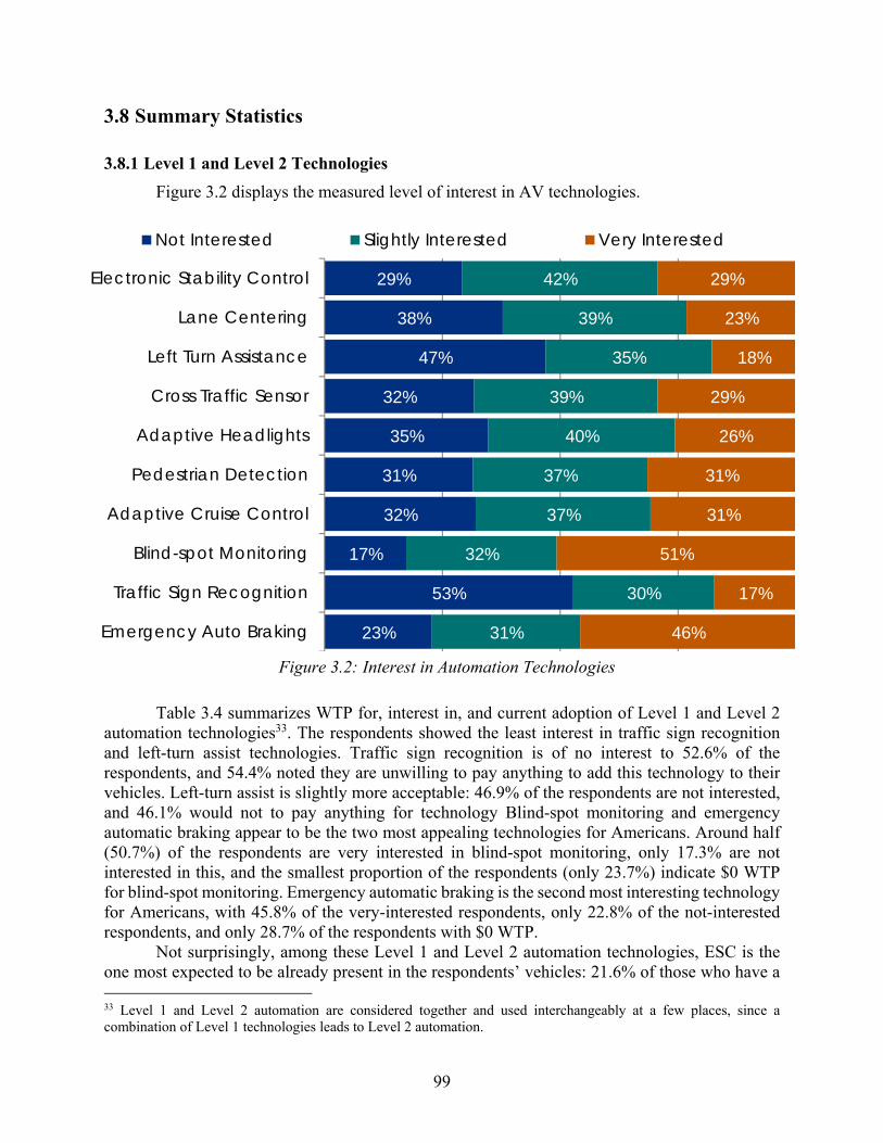
99

3.8 Summary Statistics

3.8.1 Level 1 and Level 2 Technologies

Figure 3.2 displays the measured level of interest in AV technologies.

Figure 3.2: Interest in Automation Technologies

Table 3.4 summarizes WTP for, interest in, and current adoption of Level 1 and Level 2 automation technologies33. The respondents showed the least interest in traffic sign recognition and left-turn assist technologies. Traffic sign recognition is of no interest to 52.6% of the respondents, and 54.4% noted they are unwilling to pay anything to add this technology to their vehicles. Left-turn assist is slightly more acceptable: 46.9% of the respondents are not interested, and 46.1% would not to pay anything for technology Blind-spot monitoring and emergency automatic braking appear to be the two most appealing technologies for Americans. Around half (50.7%) of the respondents are very interested in blind-spot monitoring, only 17.3% are not interested in this, and the smallest proportion of the respondents (only 23.7%) indicate $0 WTP for blind-spot monitoring. Emergency automatic braking is the second most interesting technology for Americans, with 45.8% of the very-interested respondents, only 22.8% of the not-interested respondents, and only 28.7% of the respondents with $0 WTP.

Not surprisingly, among these Level 1 and Level 2 automation technologies, ESC is the one most expected to be already present in the respondents’ vehicles: 21.6% of those who have a 33 Level 1 and Level 2 automation are considered together and used interchangeably at a few places, since a combination of Level 1 technologies leads to Level 2 automation.

29%

38%

47%

32%

35%

31%

32%

17%

53%

23%

42%

39%

35%

39%

40%

37%

37%

32%

30%

31%

29%

23%

18%

29%

26%

31%

31%

51%

17%

46%

Electronic Stability Control

Lane Centering

Left Turn Assistance

Cross Traffic Sensor

Adaptive Headlights

Pedestrian Detection

Adaptive Cruise Control

Blind-spot Monitoring

Traffic Sign Recognition

Emergency Auto Braking

Not Interested Slightly Interested Very Interested

100

vehicle reported having this technology in at least one household vehicle, and it is possible that many respondents are unaware that their vehicles now come equipped with such technology (since ESC has been mandated on all new passenger vehicles in the U.S. since 2012 model year [NHTSA 2012a]). The second most adopted technology is ACC, with 12.8% of the respondents (who have at least one vehicle) having already adopted this technology. The least adopted technology is traffic sign recognition, as it is present in only 2.1% of the respondents’ vehicles, while pedestrian detection has a slightly higher rate of adoption, at 3.3%.

The respondents’ WTP for Level 1 and Level 2 technology varies significantly34. The average WTP (among the respondents who are willing to pay some positive amount for the technology) to add ESC to an existing or a future vehicle exceeded the projected price after 5 years: $79 (see Table 3.635) versus $70. For every other technology, the average WTP (of the respondents who are ready to pay for the technology) is lower than the estimated future price after 5 years. For example, average WTP to add emergency automatic braking is $257 (versus $320, the projected price after 5 years) and for blind-spot monitoring, WTP is $210 (versus $280). The worst ratio of the average WTP to the projected price is for the adaptive headlights: $345 versus $700. Respondents value this technology significantly, and is the second most valued technology in terms of average WTP (of the respondents who are ready to pay for the technology), but respondents probably believe that the projected price is still too high.

34 Before asking a WTP question, respondents were provided with a price forecast for a particular technology. For example, the price forecast for ESC was “Current Price: $100; Price after 5 years: $70; Price after 10 years: $50.” It is difficult to estimate the price of a particular Level 1 or Level 2 technology, since these technologies are provided in packages. For example, BMW provides a $1900 package with lane departure warning, forward collision braking, ACC, pedestrian detection, and blind-spot monitoring. Thus, after analyzing different packages, current prices for each of these technologies were determined. Subsequently, a 30% price reduction in the next 5 years and a 50% price reduction in the next 10 years were considered (with 7% annual price reduction rate) to provide future price estimates of these technologies. 35 Table 3.6 demonstrates average WTP for CAV technologies. The second column represents average WTP of all respondents, and the third column summarizes the WTP of those who indicated a WTP more than $0 for a specific technology.

101

Table 3.4: Population-weighted Summaries for Level 1 and Level 2 Technologies

Response Variables Percentages Response Variables Percentages

Electronic Stability Control

Willingness to Pay to Add Present in a Vehicle*

Do not want to pay anything 33.4% Yes 21.6%

Less than $60 16.8% Interested in Technology

$60 to $79 20.4% Not interested 29.1%

$80 to $119 21.6% Slightly interested 41.6%

$120 and more 7.8% Very interested 29.3%

Lane Centering

Willingness to Pay to Add Present in a Vehicle*

Do not want to pay anything 41.7% Yes 3.9%

Less than $200 21.4% Interested in Technology

$200 to $399 14.2% Not interested 37.8%

$400 to $599 12.4% Slightly interested 39.0%

$600 and more 10.3% Very interested 23.2%

Left-Turn Assist

Willingness to Pay to Add Present in a Vehicle*

Do not want to pay anything 46.1% Yes 3.8%

Less than $100 14.9% Interested in Technology

$100 to $299 23.6% Not interested 46.9%

$300 to $399 8.1% Slightly interested 35.3%

$400 and more 7.3% Very interested 17.8%

Cross Traffic Sensor

Willingness to Pay to Add Present in a Vehicle*

Do not want to pay anything 32.8% Yes 9.6%

Less than $100 15.2% Interested in Technology

$100 to $199 14.4% Not interested 31.7%

$200 to $399 24.6% Slightly interested 38.9%

$400 and more 13.0% Very interested 29.3%

Adaptive Headlights

Willingness to Pay to Add Present in a Vehicle*

Do not want to pay anything 41.1% Yes 9.5%

Less than $150 17.7% Interested in Technology

$150 to $349 17.4% Not interested 34.7%

$350 to $649 15.2% Slightly interested 39.6%

$650 and more 8.7% Very interested 25.6%

Response Variables Perce Response Variables Percent

102

Table 3.4, continued Pedestrian Detection

Willingness to Pay to Add Present in a Vehicle*

Do not want to pay anything 37.5% Yes 3.3%

Less than $100 16.0% Interested in Technology

$100 to $199 12.8% Not interested 31.4%

$200 to $399 24.2% Slightly interested 37.1%

$400 and more 9.5% Very interested 31.5%

Adaptive Cruise Control

Willingness to Pay to Add Present in a Vehicle*

Do not want to pay anything 37.7% Yes 12.8%

Less than $150 26.2% Interested in Technology

$150 to $249 14.8% Not interested 32.1%

$250 to $349 11.9% Slightly interested 37.1%

$350 and more 9.4% Very interested 30.8%

Blind-spot Monitoring

Willingness to Pay to Add Present in a Vehicle*

Do not want to pay anything 23.7% Yes 9.9%

Less than $150 29.5% Interested in Technology

$150 to $249 18.2% Not interested 17.3%

$250 to $349 14.7% Slightly interested 31.9%

$350 and more 13.9% Very interested 50.7%

Traffic Sign Recognition

Willingness to Pay to Add Present in a Vehicle*

Do not want to pay anything 54.4% Yes 2.1%

Less than $100 15.0% Interested in Technology

$100 to $199 9.6% Not interested 52.6%

$200 to $299 10.1% Slightly interested 30.1%

$300 and more 10.9% Very interested 17.3%

Emergency Automatic Braking

Willingness to Pay to Add Present in a Vehicle*

Do not want to pay anything 28.7% Yes 5.4%

Less than $200 26.8% Interested in Technology

$200 to $299 18.3% Not interested 22.8%

$300 to $399 13.7% Slightly interested 31.5%

$400 and more 12.4% Very interested 45.8%

*Among the respondents who reported to have at least one vehicle in their households.

(Number of Observations = 2,167)

3.8.2 Connectivity and Advanced Automation Technologies

Table 3.5 summarizes respondents’ WTP to add connectivity, self-parking valet system, and Level 3 and Level 4 automation. It is evident that more than half of the respondents are not

103

ready to pay for any of the advanced automation technology, but comparatively fewer (only around 39%) indicated $0 WTP to add connectivity. Among those who are willing to pay for advanced automation, the average WTP for Level 3 automation is $5,470 and for Level 4 automation, WTP is $14,196 (see Table 3.6). Self-parking valet technology is valued at around $902 (with a simulation-projected price of $1,400 after 5 years, which may be too low [given how complex discerning a proper/legal parking spot can be in many settings]) and connectivity is valued at only $111 (projected price after 5 years is $140).

Table 3.5: Population-weighted WTP for Adding Connectivity and Advanced Automation Technologies

Response Variables Percentages Response Variables Percentages

WTP for Adding LV3 Automation WTP for Adding LV3 Valet Tech

Do not want to pay anything 55.4% Do not want to pay anything 51.7%

Less than $2,000 13.3% Less than $250 13.6%

$2,000 to $5,999 13.9% $250 to $1,249 20.1%

$6,000 to $9,999 9.4% $1,250 to $1,749 8.1%

$10,000 and more 7.9% $1,750 and more 6.5%

WTP for Adding LV4 Automation WTP for Adding Connectivity

Do not want to pay anything 58.7% Do not want to pay anything 39.1%

Less than $6,000 14.4% Less than $75 20.3%

$6,000 to $13,999 10.3% $75 to $124 16.5%

$14,000 to $25,999 9.3% $125 to $174 11.6%

$26,000 and more 7.3% $175 and more 12.5%

(Number of Observations =2,167)

Table 3.6: Population-weighted Average WTP for Automation Technologies

Average WTP for Adding Technology For all Respondents For those with WTP > 0

Electronic Stability Control $52 $79

Lane Centering $205 $352

Left-Turn Assist $119 $221

Cross Traffic Sensor $169 $252

Adaptive Headlights $203 $345

Pedestrian Detection $145 $232

Adaptive Cruise Control $126 $202

Blind-spot Monitoring $160 $210

Traffic Sign Recognition $93 $204

Emergency Automatic Braking $183 $257

Connectivity $67 $111

Self-parking Valet $436 $902

Level 3 Automation $2,438 $5,470

Level 4 Automation $5,857 $14,196

(Number of Observations =2,167)

104

3.8.3 Opinions about CAV Technologies and Related Aspects

Table 3.7 summarizes the respondents’ opinions about their own behavior, automation technologies, and related aspects. Most Americans perceive themselves as good drivers (88.2%), enjoy driving a car (75.7%), and tend to wait before adopting new technologies (79.3%). Respondents are indecisive on the topic of whether AVs will drive better than them (around one-third agrees, around one-third disagrees, and the final third has no opinion on this). Around 54.4% of the respondents perceive AVs as a useful advancement in transportation, but 58.4% are scared of them. Only around one-quarter (23.2%) of the respondents have been waiting for AV availability and only 19.5% will be comfortable sending an AV driving on its own, assuming that they as owners are liable for any accident an AV might cause. More than 41% of the respondents agree with the statement that AVs will be omnipresent in the future. Around 49% of the respondents think that AVs will function reliably, while 44% believe the idea of AVs is not realistic.

Table 3.7: Individual-weighted Opinions of Respondents

Opinions Agree Neutral Disagree

I believe that I am a very good driver myself. 88.2% 9.3% 2.6%

I think AVs will drive more safely than my driving. 33.4% 31.6% 35.0%

Driving a car is something I enjoy. 75.7% 15.4% 8.9%

I generally tend to wait for a new technology if it proves itself. 79.3% 14.2% 6.5%

AVs are a useful advance in transportation. 54.4% 26.0% 19.7%

The idea of AVs is not realistic. 43.5% 26.8% 29.7%

AVs will be a regular mode of transport in 15 years. 41.4% 32.2% 26.4%

AVs scare me. 58.4% 19.4% 22.2%

I have waited a long time for AVs. 23.2% 23.8% 53.1%

I do not think that AVs will function reliably. 49.1% 29.8% 21.2% I would be comfortable in sending my AVs out knowing that I am liable for an

id19.5% 19.9% 60.5%

(Number of Observations =2,167)

Table 3.8 summarizes the respondents’ opinions about their comfort in allowing their CVs

to share information with certain organizations or other vehicles, as well as whom they trust to develop AVs. It is interesting to note that more than half of the respondents (50.4%) are comfortable if their vehicle transmits information to other vehicles, and 42.9% are comfortable sending information to the vehicle manufacturer. Respondents were most uncomfortable sending information to insurance companies (36.4%) and toll operators (33.3%).

The respondents mostly believe that AVs must be produced by technology companies (62.3%), and luxury vehicle manufacturers (49.5%). Mass-market manufacturers are in third place with support from 45.5% of the respondents. Around 7.9% of the respondents do not trust any company to manufacture AVs, and very few respondents (1.2%) are unsure.

105

Table 3.8: Individual-weighted Opinions about Connectivity and AVs’ Production

Comfortable in allowing a vehicle to transmit information to… Comfortable Neutral Uncomfortable

Surrounding vehicles 50.4% 19.8% 29.8%

Vehicle manufacturers 42.9% 26.5% 30.6%

Insurance companies 37.0% 26.5% 36.4%

Transportation planners 40.9% 29.2% 30.0%

Toll operators 35.9% 30.9% 33.3%

To develop Level 4 AVs, I would trust: Percentage

Technology companies (e.g., Google, Apple, Microsoft, and Samsung) 62.3%

Mass-market vehicle manufacturers (e.g., Toyota and Ford) 45.5%

Luxury vehicle manufacturers (e.g., BMW and Mercedes) 49.5%

Government agencies (e.g., NASA and DARPA) 1.4%

Universities and research institutions 0.3%

I would not trust any company to develop a Level 4 AVs. 7.9%

Unsure 1.2%

(Number of Observations =2,167)

3.8.4 Opinions about AV Usage by Trip Types and Long-distance Travel

Table 3.9 demonstrates the respondents’ opinions about AV use for different trip types and long-distance travel. Interestingly, around the same proportion of the respondents reported unwillingness to use AVs for short-distance (42.5%) or long-distance (40.0%) trips (over 50 miles). Around 40% of the respondents reported their willingness to use AVs in their everyday trips; however, only one-third of the respondents plan to use them for their or their children’s school trips. In the context of long-distance travel, the highest proportion of the respondents (37.2%) plan to use AVs for trips with one-way distances between 100 and 500 miles. The respondents also believe their average number of long-distance trips will increase by 1.3 per month due to the adoption of AVs.

Table 3.9: Individual-weighted Summaries for AV Usage by Trip Type

I will use AVs during a… Percentage I will use AVs for trips… Percentage

Work trip 41.1% Between 50 and 100 miles 33.6%

School trip 33.3% Between 100 and 500 miles 37.2%

Shopping trip 42.1% Over 500 miles. 28.0%

Personal business trip 39.7% I will not use AVs for such trips. 40.0%

Social or recreational trip 44.6% Average increase in the number of long-distance trips

I will not use AVs. 42.5% Additional number of long-distance trips (per month) 1.3

(Number of Observations =2,167)

106

3.9 Forecasting Long-Term Adoption of CAV Technologies

3.9.1 Simulation-based Framework

The simulation-based framework that forecasts the long-term adoption of CAV technologies consists of several stages, pursued together in one-year intervals. The first stage is a vehicle transaction and technology adoption model (as shown in Figure 3.3) that simulates the households’ annual decisions to sell a vehicle (“sell”), buy vehicles (“buy”), sell a vehicle and buy vehicles (“replace”), add technology to the existing vehicles (“add technology”), and take no action (“do nothing”). A multinomial logit (MNL) model was estimated in BIOGEME (Bierlaire 2003) to determine the probabilities of making these decisions and use these probabilities in the Monte Carlo method to ascertain the vehicle transaction and technology adoption choice of each household after each year. Initial model specifications included all explanatory variables and the MNL model was re-estimated using stepwise elimination by removing the covariate with the lowest statistical significance. Although most of the explanatory variables enjoy a p-value greater than .05 (|z-stat| > 1.96), covariates with p-values lower than 0.32 (which corresponds to a |z-stat| of greater than 1.0) were also kept in the final specification. McFadden’s R-Square36 and adjusted R-square values are calculated to measure the models’ goodness of fit.

In the case of a “sell” decision37, the oldest vehicle (within a selling household) is disposed of. In the case of a “buy” decision, it is assumed that a household will buy (or lease) one or two vehicles, and that each vehicle can be acquired new or used. It is important to determine whether a household purchases a new or used vehicle, since it was assumed that Level 3 and Level 4 automation cannot be retrofitted into used vehicles and costs for retrofitting a self-parking valet system and Level 1/Level 2 automation into used vehicles are four times the cost of adding these technologies to new vehicles. Using the survey data, binary logit models were estimated in BIOGEME to determine these probabilities: 1) whether a household acquiring a vehicle will purchase one or two vehicles and 2) whether each vehicle will be new or used. These probabilities were used in Monte Carlo simulations.

Subsequently, connectivity is added to the purchased vehicle if a household’s WTP for connectivity is more than its price. If the purchased vehicle is used, then Level 1 and Level 2 automation are added based on the household’s total budget for Level 2 technologies, and preferences and WTP for each Level 2 technology (or Level 1 technology, if only one technology is added to the vehicle). As mentioned in Section 4.2, respondents were also separately asked about WTP for a self-parking valet system;38 this option is added to the used vehicle if the household’s WTP is more than its price. If the purchased vehicle is new and the household’s WTP for Level 4 automation is greater than the price of its addition, then Level 4 is added to the new vehicle. Otherwise a similar rule is checked for Level 3 automation. If the condition is met for Level 3, this automation is added to the new vehicle; otherwise a self-parking valet system and Level 1 and

36 McFadden’s R-Square =1 − ( ) and McFadden’s adjusted R-Square= 1 − ( ) , where n is the

number of parameters in the fitted model, and and denote the likelihood values of the fitted model and only-intercept (with no explanatory variable) model, respectively. 37 It was assumed that the household sells or disposes of only one vehicle at a time. 38 The self-parking valet system was not characterized in any level of automation, but was assumed to be present in any vehicle having Level 3 or Level 4 automation.

107

Level 2 automation are added to the new vehicle with the same rules as described for the used-vehicle case.

In the case of a “replace” decision, a household is assumed to first choose a “sell” option, followed by a “buy” decision. In the case of an “add technology” decision, if an existing vehicle already has Level 3 or Level 4 automation, then no new technology is added to the vehicle. If this is not the case, then the existing technologies in the vehicle are excluded from the choice set, and a self-parking valet system (if not present in the existing vehicle) and Level 1 and Level 2 automation are added to the existing vehicle with the same rules as described for the used-vehicle case. In the “do nothing” case, all vehicles are retained and no technology is added. If a household does not own a vehicle, but the simulation suggests it choose “sell,” “replace,” or “add technology” options, the household is forced to pick the “do nothing” option. Finally, the population-weighted adoption rates of all technologies are extracted after each year.

This simulation framework does not consider the changes in household demographics over time (except the respondent’s age and vehicle ownership, since they are explanatory variables in the vehicle transaction and technology adoption model). Integrating these additional household evolution models may improve estimates of CAV technologies’ future adoption rates.

108

Figure 3.3: The Simulation-based Framework to Forecast Long-term Technology Adoption

3.9.2 Vehicle Transaction and Technology Adoption: Model Specifications

Table 3.10 summarizes (with population weights) person- and household-level variables, geocoded location variables, and transaction decision variables included in the vehicle transaction and technology adoption models.

109

Table 3.10: Population-weighted Summary Statistics of Explanatory Variables

Explanatory Variables Mean SD Min. Max.

Person Variables

Age (years) 44.980 16.623 21 70

Male? 0.4897 0.5000 0 1

Single? 0.3358 0.4724 0 1

Bachelor’s degree holder? 0.2561 0.4366 0 1

Full-time worker? 0.3146 0.4645 0 1

Have U.S. driver license? 0.9045 0.2940 0 1

Disabled? 0.1285 0.3348 0 1

Annual vehicle-miles traveled over 9,000 miles? 0.3971 0.4894 0 1

Retired? 0.1848 0.3882 0 1

Drive alone for work trips? 0.5151 0.4999 0 1

Household Variables

More than 3 members in the household? 0.2553 0.4361 0 1

Number of workers in the household 1.1944 0.9220 0 7

More than 1 worker in the household? 0.3491 0.4768 0 1

Household income 64,640 51,924 5,000 250,000

Age of the oldest vehicle in the household (in years) 10.661 7.3239 0 30

Number of vehicles owned by the household 1.7828 1.0176 0 6

At least one vehicle in the household? 0.9292 0.2566 0 1

Number of vehicles sold in the past 10 years 0.4230 0.6651 0 5

At least one vehicle sold in the past 10 years? 0.3488 0.4767 0 1

Location Variables

% of families below poverty line in the census tract 12.301 10.155 0 77

Employed and over 16 years of age (per square mile) 2,826.0 6,232.6 1.1917 1,13,187

Population density (per square mile) 3,958.8 8,680.4 1.6496 1,32,409

Distance to transit stop (from home) is greater than 3 miles? 0.4868 0.4999 0 1

Distance to downtown (from home) is greater than 5 miles? 0.6428 0.4793 0 1

Response Variables Mean SD Min. Max.

Transaction Decisions

Sell 0.0382 0.1916 0 1

Replace 0.2406 0.4276 0 1

Buy 0.1639 0.3703 0 1

Add technology 0.0890 0.2848 0 1

Do nothing 0.4683 0.4991 0 1

Bought Two Vehicles? 0.0766 0.2659 0 1

Bought New Vehicle? 0.6495 0.4771 0 1

(Number of Observations =2,167)

110

Table 3.11 shows the transaction model’s final specification. The alternative specific constants (ASCs) indicate that, everything else being equal, households have inherent inclination and disinclination for “buy” and “replace” options. Specifically, older and single individuals with more than one worker in the household, who live farther from downtown in a financially poorer neighborhood (all other attributes remaining constant), are relatively less inclined towards selling their vehicles, but males with more vehicles in the household are likely to be more inclined to sell.

Bachelor’s degree holders, full-time workers, and male respondents who drive alone for work, have more vehicles, and have more than one worker in the household are more likely (everything else held constant) to replace a vehicle, but older respondents are less likely to make this decision. Older and single respondents whose households own more vehicles (all other attributes held constant) are less likely to buy vehicles. In contrast, respondents who drive alone to work, have more than three members and one worker in the household, and have older vehicles are more likely to buy vehicles. It is interesting to note that bachelor’s degree holders who drive alone for work trips and live in neighborhoods with higher density of employed individuals are more inclined (everything else held constant) towards the “add technology” option than the “do nothing.” However, all else being equal, older individuals who have older vehicles are likely to prefer the “do nothing” option over the “add technology.”

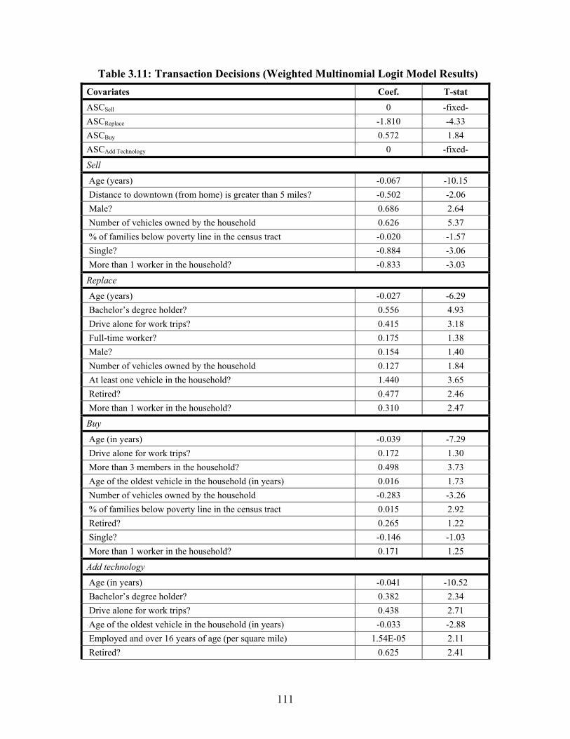
111

Table 3.11: Transaction Decisions (Weighted Multinomial Logit Model Results)

Covariates Coef. T-stat

ASCSell 0 -fixed-

ASCReplace -1.810 -4.33

ASCBuy 0.572 1.84

ASCAdd Technology 0 -fixed-

Sell

Age (years) -0.067 -10.15

Distance to downtown (from home) is greater than 5 miles? -0.502 -2.06

Male? 0.686 2.64

Number of vehicles owned by the household 0.626 5.37

% of families below poverty line in the census tract -0.020 -1.57

Single? -0.884 -3.06

More than 1 worker in the household? -0.833 -3.03

Replace

Age (years) -0.027 -6.29

Bachelor’s degree holder? 0.556 4.93

Drive alone for work trips? 0.415 3.18

Full-time worker? 0.175 1.38

Male? 0.154 1.40

Number of vehicles owned by the household 0.127 1.84

At least one vehicle in the household? 1.440 3.65

Retired? 0.477 2.46

More than 1 worker in the household? 0.310 2.47

Buy

Age (in years) -0.039 -7.29

Drive alone for work trips? 0.172 1.30

More than 3 members in the household? 0.498 3.73

Age of the oldest vehicle in the household (in years) 0.016 1.73

Number of vehicles owned by the household -0.283 -3.26

% of families below poverty line in the census tract 0.015 2.92

Retired? 0.265 1.22

Single? -0.146 -1.03

More than 1 worker in the household? 0.171 1.25

Add technology

Age (in years) -0.041 -10.52

Bachelor’s degree holder? 0.382 2.34

Drive alone for work trips? 0.438 2.71

Age of the oldest vehicle in the household (in years) -0.033 -2.88

Employed and over 16 years of age (per square mile) 1.54E-05 2.11

Retired? 0.625 2.41

112

Table 3.11, continued Fit statistics Null log-likelihood -3487.65 Final log-likelihood -2688.66 McFadden’s R-square 0.229 Adjusted R-square 0.220 Number of observations 2,167

Note: The “do nothing” option is base here.

Table 3.12 shows the “bought two vehicles?” model’s final specification. Male and disabled respondents whose households sold more vehicles in the past 10 years, have more workers, and live farther from transit stops in highly populous neighborhoods (with everything else held constant) are more likely to purchase two vehicles. However, single respondents who travel more and live in poorer neighborhoods are inclined to buy only one vehicle.

Table 3.12: Bought Two Vehicles? (Binary Logit Model Results)

Covariates Coef. T-stat

Constant -3.019 -6.74

Number of vehicles sold in the past 10 years 0.412 2.07

Distance to transit stop (from home) is greater than 3 miles? 0.527 1.67

Distance to downtown (from home) is greater than 5 miles? -0.324 -1.01

Annual vehicle-miles traveled over 9,000 miles? -0.552 -1.88

Disabled? 0.670 1.68

Number of workers in the household 0.335 1.87

Male? 0.460 1.63

Population density (per square mile) 2.62E-05 3.91

% of families below poverty line in the census tract -0.021 -1.54

Single? -0.744 -2.15

Fit statistics

Null log-likelihood -279.24

Final log-likelihood -257.68

McFadden’s R-square 0.077

Adjusted R-square 0.074

Number of observations 1033

Table 3.13 shows the “bought new vehicle?” model’s final specification. Older, licensed

drivers, full-time workers, and male respondents whose households own more vehicles, have higher income, and live in neighborhoods with a higher density of employed individuals (all other attributes held constant) are more inclined towards buying new vehicles. In contrast, disabled respondents who: have more workers in the household; sold at least one vehicle in the past 10 years; and live in highly populous neighborhoods; are more likely to buy used vehicles.

The respondent’s age, number of vehicles owned by the household, number of vehicles sold in the past 10 years, indicator for owning at least one vehicle, indicator for selling at least one vehicle in the past 10 years, and age of the oldest vehicle in the household are annually updated in the simulation.

113

Table 3.13: Bought New Vehicle? (Binary Logit Model Results)

Covariates Coef. T-stat

Constant -2.584 -3.53

Number of vehicles owned by the household 0.418 2.17

At least one vehicle in the household? 2.304 4.32

Age of the oldest vehicle in the household (in years) -0.093 -4.39

Number of vehicles sold in the past 10 years 0.535 2.01

At least one vehicle sold in the past 10 years? -2.162 -5.12

Disabled? -0.639 -1.51

Number of workers in the household -0.462 -2.98

Age (years) 0.011 1.41

Male? 0.349 1.44

Have U.S. driver license? 0.774 1.25

Household income 1.45E-05 4.25

Full-time worker? 0.708 2.73

Population density (per square mile) -3.41E-05 -1.35

Employed and over 16 years of age (per square mile) 4.41E-05 1.29

Fit statistics

Null log-likelihood -467.04

Final log-likelihood -340.71

McFadden’s R-square 0.270

Adjusted R-square 0.262

Number of observations 721

3.9.3 Forecasted Adoption Rates of CAV Technologies under WTP, Pricing, and Regulation Scenarios

Description of Scenarios

This simulation forecasts the annual adoption rates39 of CAV technologies over the next 30 years (2016 to 2045) under eight different scenarios based on WTP, technology price, and NHTSA regulations (see Table 3.14).

As indicated in Tables 3.1 and 3.2, many respondents do not want to pay anything to add CAV technologies. For example, more than 50% of respondents have $0 WTP to add Level 3 and Level 4 automation. Perhaps these respondents are not able to conceive a world with only CAVs and also may have various safety and reliability concerns about the technology. As the public learns more about CAVs and more people gain familiarity with these technologies, these perceptions and potential behavioral responses are apt to change, in some cases rapidly. In Scenario 1, the original WTP (as reported by the respondents) was considered and assumed constant over time. However, for all other scenarios (2 to 8), respondents who reported $0 WTP were assigned

39 Technology adoption rate refers to the percentage of vehicles (population-weighted) having a specific technology. Vehicles with Level 3 and Level 4 automation are assumed to have all Level 1 and Level 2 automation technologies.

114

a non-zero WTP40 for year 2015, and their assigned WTPs (the 10th percentile value of all non-zero-WTP respondents in their demographic cohort) rose over time, at the same rate as everyone else’s WTP.

Scenarios 1 and 2 do not consider any NHTSA current and probable technology adoption regulations, but the remaining scenarios (3 to 8) assume mandatory adoption of ESC from year 201541 and connectivity from year 202042 on all new vehicles.

Table 3.14: WTP Increase, Tech-Pricing Reduction, and Regulation Scenarios

Scenario Annual WTP increment rate Annual Tech-price Reduction Rate Regulations 1 0% 10% No 2 0%, but no zero WTP values 10% No 3 0%, but no zero WTP values 5% Yes 4 0%, but no zero WTP values 10% Yes 5 5% 5% Yes 6 5% 10% Yes 7 10% 5% Yes 8 10% 10% Yes

As mentioned earlier, it is difficult to estimate the price of a particular Level 1 or Level 2

technology since automobile companies provide these technologies in packages. Thus, current prices for these technologies are approximately estimated by analyzing packages provided by BMW, Mercedes, and other manufacturers. Prices to add connectivity, Level 3, and Level 4 automation were estimated based on experts’ opinions. Table 3.15 shows an example of temporal variation of the prices to add CAV technologies to the new vehicles43 at the assumed annual price reduction rate of 5%.

40 To assign WTP to the respondents who do not want to pay anything for a specific technology, the sample was classified into 40 categories (based on household size, number of workers, and household vehicle ownership). Subsequently, a household that does not want to pay anything for specific technology was assigned a WTP of the 10th percentile of all non-zero WTP values in the household’s category. 41 ESC has been mandated on all new passenger vehicles in the U.S. since the 2012 model year (NHTSA 2012). 42 NHTSA is expected to require connectivity on all vehicles produced after year 2020 (Automotive Digest 2014). 43 In this study, costs for retrofitting a self-parking valet system, Level 1, and Level 2 automation into the used vehicles are assumed to be four times the cost of adding these technologies to new vehicles. For example, as per Table 3.12, the cost to add traffic sign recognition to the new vehicle is $450, but the cost for retrofitting it into a used vehicle is assumed to be $1800.

115

Table 3.15: Technology Prices at 5% Annual Price Reduction Rates

Technology 2015 2020 2025 2030 2035 2040 2045

Electronic Stability Control 100 77.4 59.9 46.3 35.8 27.7 21.5 Lane Centering 950 735.1 568.8 440.1 340.6 263.5 203.9 Left-turn assist 450 348.2 269.4 208.5 161.3 124.8 96.6 Cross Traffic Sensor 550 425.6 329.3 254.8 197.2 152.6 118.1 Adaptive Headlights 1,000 773.8 598.7 463.3 358.5 277.4 214.6 Pedestrian Detection 450 348.2 269.4 208.5 161.3 124.8 96.6 Adaptive Cruise Control 400 309.5 239.5 185.3 143.4 111.0 85.9 Blind-spot Monitoring 400 309.5 239.5 185.3 143.4 111.0 85.9 Traffic Sign Recognition 450 348.2 269.4 208.5 161.3 124.8 96.6 Emergency Automatic Braking 450 348.2 269.4 208.5 161.3 124.8 96.6 Connectivity 200 154.8 119.7 92.7 71.7 55.5 42.9 Self-parking Valet 2,000 1,547.6 1,197.5 926.6 717.0 554.8 429.3 Level 3 Automation 15,000 11,606.7 8,981.1 6,949.4 5,377.3 4,160.8 3,219.6 Level 4 Automation 40,000 30,951.2 23,949.5 18,531.6 14,339.4 11,095.6 8,585.6

Overall Comparison of Technology Adoption in Eight Scenarios

Tables 3.16 to 3.19 present the estimated/simulated ownership rates (across all privately held light-duty vehicles, not just new vehicles being sold) at 5-year intervals, across the eight scenarios. Substantial differences are visible between the long-term adoption rates of all technologies (except Level 3 and Level 4 automation)44 in Scenarios 1 (constant WTP) and 2 (constant WTP, but no zero WTP values45). For example, in 2045, connectivity’s adoption rate is 59.5% in Scenario 1 and 83.5% in Scenario 2. Such differences emerged because a large proportion of households cannot adopt some technologies in Scenario 1, even at very low prices due to their WTP of $0.

The regulations’ (regarding adoption of ESC and connectivity) effect on CAV technologies’ adoption rates can be observed by comparing the results of Scenario 2 (see Table 3.16) and Scenario 4 (see Table 3.17), since WTP and technologies prices have the same dynamics in both scenarios. In Scenario 2 (no regulations), ESC and connectivity have adoption rates of 43.8% and 35.2% in 2025, but these numbers increase to 98.4% and 88.4%, respectively, due to incorporation of regulations in Scenario 4.

The technology-pricing impacts on the adoption of CAV technologies can be visualized by comparing adoption rates in Scenarios 3 and 4 (or 5 and 6, or 7 and 8), since these scenarios include regulations and have the same temporal variations in WTP, but different tech-price variations. Table 3.17 shows that most of the technologies’ long-term adoption rates under an annual 10% tech-price reduction (Scenario 4) are much higher46 than those under a 5% price-reduction

44 In Scenario 2, all respondents with $0 WTP are assigned non-zero WTP values, but new WTP values are not enough to make advanced automation technologies affordable, even at 10% price drop rates. Thus, Level 3 and Level 4 automation adoption rates differ very little between Scenarios 1 and 2. 45 No-zero WTP implies that there is no household in the sample with $0 WTP for any technology, since the sample has been corrected for this bias, as discussed above. 46 However, for a few technologies, adoption rates are lower in Scenario 4 as compared to Scenario 3 at some point in time. For example, ESC’s adoption rates (in 2025) are 98.6% in Scenario 3 and 98.4% in Scenario 4. These minor unintuitive differences might have occurred due to the noise of the simulation involving random number generation.

116

(Scenario 3), since technologies are obviously affordable for many more households in Scenario 4 as compared to Scenario 3. For example, in 2045, Level 4 automation’s adoption rates are 24.8% in Scenario 3 and 43.4% in Scenario 4.

The effect of WTP increments on CAV technologies’ adoption rates can be observed by comparing the results of Scenarios 4, 6, and 8 (or 3, 5, and 7), since these scenarios incorporate NHTSA regulations, and the same temporal variations of technology pricing, but different WTP variations. As expected, the following tables demonstrate that, for most of the technologies, the long-term adoption rates in 0%, 5%, and 10% WTP increment scenarios show corresponding increases. For example, in 2045, Level 4 automation’s adoption rates in Scenarios 4, 6, and 8 are 43.4%, 70.7%, and 87.2%, respectively. Figure 3.4 provides an illustration of the estimated shares of U.S. light-duty vehicles with advanced automation.

117

Table 3.16: Estimated Shares of US Light-Duty Vehicles with CAV-related Technologies in Scenarios 1 and 2

Technology Scenario 1: Constant WTP, 10% drop in tech-prices, and no regulation Scenario 2: No-zero-WTP, 10% tech-price drop, and no regulation

2015 2020 2025 2030 2035 2040 2045 2015 2020 2025 2030 2035 2040 2045 Electronic Stability Control 24.3 25.3 33.2 43.3 52.7 58.2 63.8 24.3 32.3 43.8 61.2 76.7 83.2 92.9 Lane Centering 4.4 8.3 18.9 31.0 40.8 48.8 56.8 4.4 8.6 20.2 33.5 45.9 55.2 68.8 Left-turn assist 3.8 9.9 20.1 32.4 41.8 50.3 58.1 3.8 10.4 21.8 35.1 47.2 65.6 80.2 Cross Traffic Sensor 10.9 12.9 22.6 35.1 45.1 52.6 60.3 10.9 13.8 25.9 41.1 53.7 66.0 82.8 Adaptive Headlights 10.2 9.7 18.8 30.9 41.0 49.2 58.0 10.2 9.8 19.8 32.4 46.2 55.9 77.5 Pedestrian Detection 3.7 10.6 21.7 34.5 44.1 52.6 59.8 3.7 11.2 24.1 38.2 50.3 69.1 82.8 Adaptive Cruise Control 13.3 14.9 24.1 35.2 44.7 52.2 59.8 13.3 16.2 27.0 40.1 53.4 62.2 76.1 Blind-spot Monitoring 11.7 15.0 26.1 38.5 48.2 55.1 62.1 11.7 17.3 31.9 46.3 59.7 67.8 80.7 Traffic Sign Recognition 2.0 7.7 18.0 30.0 39.8 48.9 57.0 2.0 7.6 18.4 31.4 43.5 63.3 78.6 Emergency Automatic Braking 5.6 11.8 24.4 37.1 46.9 54.6 61.6 5.6 11.8 26.4 43.7 57.7 74.3 86.2 Connectivity 0 17.7 34.8 44.7 51.1 53.0 59.5 0 18.0 35.2 46.1 57.6 61.4 83.5 Self-parking Valet 0 9.1 21.4 33.9 45.1 52.5 61.2 0 9.2 21.6 34.5 46.3 54.4 73.5 Level 3 Automation 0 2.1 4.6 7.6 8.3 8.0 10.4 0 3.0 5.3 7.7 8.7 7.9 13.7 Level 4 Automation 0 3.9 11.1 19.7 28.6 37.0 43.0 0 3.0 10.2 19.0 28.7 37.9 43.8

118

Table 3.17: Estimated Shares of US Light-Duty Vehicles with CAV-related Technologies in Scenarios 3 and 4

Technology Scenario 3: No-zero-WTP, 5% drop in tech-prices, and regulations Scenario 4: No-zero-WTP, 10% drop in tech-prices, and regulations

2015 2020 2025 2030 2035 2040 2045 2015 2020 2025 2030 2035 2040 2045 Electronic Stability Control 24.3 88.9 98.6 99.8 100 100 100 24.3 89.1 98.4 99.9 100 100 100 Lane Centering 4.4 6.1 12.0 19.7 27.1 33.1 40.7 4.4 8.5 19.9 33.0 45.5 53.9 66.5 Left-turn assist 3.8 7.9 14.2 21.3 28.1 35.1 42.5 3.8 10.0 21.8 35.0 46.5 60.6 75.1 Cross Traffic Sensor 10.9 11.7 16.8 22.9 31.9 39.1 47.4 10.9 13.7 25.4 39.8 52.2 62.2 76.8 Adaptive Headlights 10.2 7.6 11.2 18.3 26.4 32.6 39.9 10.2 9.5 19.6 32.3 46.1 53.6 71.6 Pedestrian Detection 3.7 8.3 15.0 23.2 30.7 38.3 45.5 3.7 10.7 24.0 37.5 49.7 63.4 77.1 Adaptive Cruise Control 13.3 13.2 18.4 25.7 33.2 39.2 46.5 13.3 16.5 28.1 39.7 53.0 60.4 73.4 Blind-spot Monitoring 11.7 13.8 20.3 29.7 39.6 45.7 53.5 11.7 16.5 31.6 45.6 59.1 66.0 77.2 Traffic Sign Recognition 2.0 5.4 10.5 17.7 24.9 31.4 38.1 2.0 7.3 18.2 30.9 42.7 58.7 73.9 Emergency Automatic Braking 5.6 8.6 15.6 26.1 34.7 43.4 51.2 5.6 12.3 26.3 42.3 57.2 69.1 80.9 Connectivity 0 36.5 88.2 98.4 99.7 100 100 0 41.3 88.4 98.4 99.7 100 100 Self-parking Valet 0 6.0 13.1 20.9 29.0 34.9 41.6 0 9.2 21.1 33.4 45.7 53.4 71.9 Level 3 Automation 0 1.9 3.2 4.5 6.5 8.1 8.9 0 2.7 5.1 7.5 8.7 8.2 13.9 Level 4 Automation 0 2.0 5.2 10.3 15.0 19.2 24.8 0 2.9 10.2 18.8 28.5 36.3 43.4

119

Table 3.18: Estimated Shares of US Light-Duty Vehicles with CAV-related Technologies in Scenarios 5 and 6

Technology Scenario 5: 5% rise in WTP, 5% drop in tech-price, and regulations Scenario 6: 5% rise in WTP, 10% drop in tech-price, and regulations

2015 2020 2025 2030 2035 2040 2045 2015 2020 2025 2030 2035 2040 2045 Electronic Stability Control 24.3 89.1 98.3 99.9 100 100 100 24.3 88.7 98.2 99.9 100 100 100 Lane Centering 4.4 8.5 21.1 33.5 43.5 53.1 59.8 4.4 10.3 26.8 44.5 56.5 81.4 92.9 Left-turn assist 3.8 10.3 22.0 35.0 44.4 59.2 71.5 3.8 11.9 27.8 44.8 66.2 88.1 96.3 Cross Traffic Sensor 10.9 14.3 25.7 39.6 50.6 60.9 73.4 10.9 15.7 32.1 50.2 68.9 87.3 96.3 Adaptive Headlights 10.2 10.0 20.5 32.3 43.4 53.0 67.1 10.2 11.0 26.4 44.5 63.4 84.8 95.4 Pedestrian Detection 3.7 11.1 24.5 38.1 47.9 61.4 74.0 3.7 13.2 30.9 48.5 68.6 88.6 96.5 Adaptive Cruise Control 13.3 16.1 27.4 39.4 51.8 60.3 68.3 13.3 18.3 33.9 51.5 66.7 86.4 95.8 Blind-spot Monitoring 11.7 17.5 30.8 44.6 57.5 66.3 73.6 11.7 17.8 37.7 57.3 71.6 88.4 96.3 Traffic Sign Recognition 2.0 7.1 19.0 30.7 41.4 56.5 70.0 2.0 8.6 24.5 41.0 63.8 87.3 96.2 Emergency Automatic Braking 5.6 11.6 26.4 42.4 54.6 67.3 77.8 5.6 14.1 34.2 55.0 73.3 91.0 97.2 Connectivity 0 39.1 89.3 98.5 99.8 100 100 0 40.5 88.8 98.2 99.7 100 100 Self-parking Valet 0 8.6 21.8 34.0 44.4 52.4 67.1 0 10.2 26.9 44.2 64.5 85.6 96.5 Level 3 Automation 0 2.3 5.3 8.1 8.5 8.3 8.2 0 2.1 6.1 8.4 8.5 28.6 16.3 Level 4 Automation 0 3.3 10.8 19.0 27.2 35.9 43.2 0 4.7 15.1 27.2 38.3 45.7 70.7

120

Table 3.19: Estimated Shares of US Light-Duty Vehicles with CAV-related Technologies in Scenarios 7 and 8

Technology Scenario 7: 10% rise in WTP, 5% drop in tech-price, and regulations Scenario 8: 10% rise in WTP, 10% drop in tech-price, and regulations

2015 2020 2025 2030 2035 2040 2045 2015 2020 2025 2030 2035 2040 2045 Electronic Stability Control 24.3 89.7 98.1 99.8 100 100 100 24.3 89.1 98.8 99.9 100 100 100 Lane Centering 4.4 10.8 25.5 42.1 55.1 78.1 90.3 4.4 13.5 32.8 51.2 79.0 94.0 97.9 Left-turn assist 3.8 11.6 26.5 43.0 65.1 83.6 95.0 3.8 14.1 34.1 60.9 87.3 96.4 98.4 Cross Traffic Sensor 10.9 15.6 30.8 48.3 65.4 84.6 95.0 10.9 18.2 39.3 63.6 87.0 96.6 98.5 Adaptive Headlights 10.2 11.4 25.0 42.3 58.5 81.3 92.5 10.2 13.4 32.8 55.8 81.4 95.5 98.2 Pedestrian Detection 3.7 12.9 28.8 45.8 67.9 84.6 95.3 3.7 15.3 37.6 63.7 87.9 96.8 98.7 Adaptive Cruise Control 13.3 18.0 31.7 49.1 62.5 82.8 92.8 13.3 20.3 40.4 60.2 83.2 95.4 98.2 Blind-spot Monitoring 11.7 18.5 35.6 54.6 67.7 85.4 94.0 11.7 20.5 45.5 66.4 85.9 96.3 98.6 Traffic Sign Recognition 2.0 9.0 23.2 39.0 62.0 82.6 94.9 2.0 10.9 30.0 57.9 86.4 96.4 98.4 Emergency Automatic Braking 5.6 13.9 32.9 52.1 72.4 88.0 96.4 5.6 16.6 41.5 68.4 90.0 97.3 98.9 Connectivity 0 41.8 89.1 98.3 99.7 100 100 0 41.3 89.4 99.0 99.9 100.0 100.0 Self-parking Valet 0 10.5 25.5 41.6 57.6 82.4 92.9 0 12.6 32.9 54.6 80.3 96.0 99.4 Level 3 Automation 0 2.5 5.9 8.3 8.2 26.5 25.5 0 3.5 6.0 7.7 27.7 11.6 2.9 Level 4 Automation 0 4.7 13.8 25.5 36.4 44.3 59.7 0 5.5 19.4 33.8 44.2 74.7 87.2

121

Level 3 Automation Self-parking Valet

Level 4 Automation Connectivity

Figure 3.4: Estimated Shares of US Light-Duty Vehicles with Advanced Automation

10.4%13.7%

8.9%

13.9%

8.2%

16.3%25.5%

0.0%2.9%0%

25%

50%

75%

100%

2015 2020 2025 2030 2035 2040 2045

61.2%

73.5%

41.6%

71.9%67.1%

96.5%92.9%

0.0%

99.4%

0%

25%

50%

75%

100%

2015 2020 2025 2030 2035 2040 2045

43.0%

43.8%

24.8%

43.4%43.2%

70.7%59.7%

0.0%

87.2%

0%

25%

50%

75%

100%

2015 2020 2025 2030 2035 2040 2045

59.5%

83.5%100.0%100.0%100.0%100.0%100.0%

0.0%

100.0%

0%

25%

50%

75%

100%

2015 2020 2025 2030 2035 2040 2045

122

Adoption Rates of Connectivity, Level 1 and Level 2 Technologies

It is interesting to note that around 98% of the vehicle fleet is likely to have ESC and connectivity in years 2025 and 2030, respectively, under NHTSA’s current and probable regulations (Scenarios 3 to 8). However, it is worth noting that in case of no regulations, even at a 10% annual drop in tech prices and no zero WTP values (Scenario 2), 92.9% of vehicles would have ESC and 83.5% would have connectivity in 2045 (see Table 3.16). NHTSA’s regulations are likely to accelerate adoption of these technologies by 15 to 20 years, and make U.S. roads safer.

In Scenario 6 (5% rise in WTP and 10% drop in technology prices each year), Scenario 7 (10% rise in WTP and 5% drop in tech-prices), and Scenario 8 (10% rise in WTP and 10% drop in technology prices annually), all Level 1 technologies are estimated to have more than 90% adoption rates in 2045. Adoption rates of Level 1 technologies are further explored in Scenario 3 (5% drop in tech-prices and no zero WTP values) and Scenario 5 (5% rise in WTP and 5% drop in tech-prices). Traffic sign recognition is the least adopted and least appealing Level 1 technology in 2015, and is anticipated to remain least adopted, with adoption rates of 38.1% in 2045 in Scenario 3, but fourth-least adopted (out of nine, excluding ESC) with adoption rates of 70% in Scenario 547. Section 4.2 suggests that blind-spot monitoring and emergency automatic braking are the two most appealing Level 1 technologies for Americans. These technologies are anticipated to be the most and second-most adopted Level 1 technologies (excluding ESC) in 2045 in Scenario 3, with adoption rates of 53.5% and 51.2%, but are the third-most and most adopted Level 1 technologies in Scenario 5, with adoption rates of 73.6% and 77.8%. Pedestrian detection is the second-least adopted technology in 2015, but is expected to be the second-most adopted Level 1 technology (out of nine, excluding ESC) in 2045 in Scenario 5, with an adoption rate of 74.0%.

Adoption Rates of Advanced Automation Technologies

It is interesting to note that as WTP increases and tech prices drop, Level 4 automation adoption rates shoot up while, at the same time, Level 3 automation adoption rates decrease. For example, in 2045, Level 3 and Level 4 adoption rates are forecasted to be 8.2% and 43.2% in Scenario 5 (5% drop in tech-prices and 5% WTP rise), which change to 2.9% and 87.2% in Scenario 8 (10% drop in tech-prices and 10% WTP rise). This trend occurs because the simulation framework first checks whether a new-vehicle-buyer household can afford Level 4 automation (WTP exceeds the technology’s price) in that specific year. If a household can, then Level 4 automation is added to the new vehicle; otherwise, the same rule is checked for Level 3. So, with the increase in WTP or/and reduction in technology prices, many households will be able to afford Level 4 vehicles. Thus, due to this hierarchical framework, Level 3 automation is automatically skipped in those choice sets. Self-parking valet system is likely to be adopted by 34.0% to 54.6% of the vehicle fleet in 2030 and 67.1% to 99.4% of the 2045 vehicle fleet48.

47 Lane centering is the least adopted Level 1 technology in Scenario 5 in 2045, with an adoption rate of 59.8%. 48 Lower bounds on adoption rates are anticipated for Scenario 5 (5% drop in tech-prices and 5% WTP rise) and upper bounds are forecasted for Scenario 8 (10% drop in tech-prices and 10% WTP rise).

123

3.10 Assessing Texans’ Opinions about and WTP for Automation and Connected Vehicle Technologies

3.10.1 Survey Design and Data Processing

Questionnaire Design and Data Acquisition

The team designed and disseminated another Texas-wide survey in June 2015 using Qualtrics, a web-based survey tool, following the same protocol outlined in Section 4.1 for the national survey.

Exploring respondents’ opinions and preferences for the adoption of emerging vehicle and transport technologies, the survey asked 93 questions, divided into 7 sections. Respondents were asked about their opinions about AVs (e.g., concerns and benefits of AVs), crash history and opinions about speed regulations49 (e.g., number of moving violations, and support for red light cameras and automated speed enforcement), and their WTP for and interest in various Level 1 and 2 technologies (e.g., adaptive headlights and ACC). Respondents were also asked about their WTP for and interest in CVs (e.g., road sign information using a head-up display), adoption rates of carsharing, transportation network companies’ (TNC’s) services (like UberX and Lyft) and SAVs, their households’ home-location shifting decisions (once AVs and SAVs become common modes of transport), opinions about congestion pricing strategies (e.g., toll if revenue is evenly distributed among residents), travel patterns (e.g., AVs’ usage by trip purpose and distance from city’s downtown), and demographics.

Data Cleaning and Sample Correction

A total of 1,297 Texans completed the survey, but after removing the fast responses and conducting some sanity checks50, 1,088 responses remained eligible for further analysis. The sample over-represented specific demographic classes, such as men older than 65 years and bachelor’s degree holders, and under-represented others, such as individuals who did not complete high school and men 18 to 24 years old. Therefore, the survey sample proportions in 3 demographic classes or 60 categories (2 gender-based, 5 age-based, and 6 educational-attainment groups) were scaled using the 2013 American Community Survey’s PUMS for Texas51. These scale factors were used as person-level weights to un-bias person-related summary statistics (e.g., concerns related

49 Respondents’ crash history and opinions about speed law enforcement were asked to explore correlation of such attributes with their opinions of and WTP for CAV technologies. 50 Respondents who completed the survey in less than 15 minutes were assumed to have not read questions thoroughly, and their responses were discarded. Respondents were provided with NHTSA’s automation levels’ definitions and, subsequently, were asked whether they understood this description or not. Those who did not understand it (5.7%, or 65 respondents) were considered ineligible for further analysis. Certain other respondents were also considered ineligible for further analysis: those younger than 18 years of age, reporting more workers or children than the household size, reporting the same distance of their home from various places (airport and city center, for example), and providing other combinations of conflicting answers. 51 Two categories—“Master’s degree holder female and 18 to 24 years old” and “Master’s degree holder male and 18 to 24 years old”—were missing in the sample data. These categories were merged with “Bachelor’s degree holder female and 18 to 24 years old” and “Bachelor’s degree holder male and 18 to 24 years old,” respectively, in the population.

124

to AVs) and model-based parameter estimates (e.g., binary opinion of whether or not to allow 13- to 15-year-old children to ride alone in AVs).

Similarly, some household groups were under- or over-represented. Thus, household weights were calculated for 3 demographic classes or 26 categories (4 household size groups, 4 household workers groups, and 2 vehicle ownership groups)52 using PUMS 2013 data. These household weights were used to un-bias household-related (e.g., WTP for new technologies and vehicle transaction decisions) model estimates and summary statistics.

Geocoding

To understand the spread of survey respondents across Texas and to account for the impact of built-environment factors (e.g., population density and population below poverty line) on respondents WTP for and opinions about CAV technologies, the respondents’ home addresses were geocoded using Google Maps API and spatially joined with Texas’s census-tract-level shape file using open-source Quantum GIS. For respondents who did not provide their street address or recorded incorrect addresses, their internet protocol (IP) locations were used as the proxies for their home locations. Figure 3.5 shows the geocoded respondents across Texas, with most respondents living in or around Texas’s biggest cities (Houston, Dallas, Fort Worth, San Antonio, and Austin), as expected in a relatively unbiased sample.

Figure 3.5: Geocoded Respondents across Texas

Dataset Statistics

Table 3.20 summarizes all explanatory variables used in several model calibrations of this study. These are grouped into six categories, based on these predictors: person, household,

52 There are 32 combinations of traits (4 x 4 x 2 = 32), but there are only 26 categories because some of the categories cannot exist. For example, the number of workers cannot exceed household size. A category “household with more than three members, more than two workers, and no vehicle” was missing and was merged with “household with more than three members, two workers, and no vehicle” in the population.

125

location, travel, technology, and safety. Person- and household-based weights, as appropriate, were employed in calculating summary statistics and model calibration to correct for sample biases.

3.10.2 Texans’ Technology-awareness and Safety-related Opinions

Technology-based predictors provide key insights about Texans’ attitude towards new technologies. Around 77% of (population-weighted) Texans use a smartphone and a bit more than a half (59%) know about the existence of Google self-driving cars; however, only 19% have ever heard about CVs (before participating in the survey). Surprisingly, around two-thirds are familiar with TNC’s services like UberX and Lyft, but only 25% are aware about the carsharing programs. Only 7% of respondents’ households own at least a modern vehicle with Level 2 automation.

Texans’ attitudes towards safety-regulation strategies, crash history, and moving violation history are captured in the safety-based predictors. Around half of the respondents support each of these speed regulation strategies: red light cameras, automated speed enforcement, and speed governors. On average, Texans have experienced 0.25 crashes involving fatalities or serious injuries and 0.7 crashes involving monetary losses in past 15 years. Each respondent received at least one moving violation within past ten years, on average, while 20% received more than one violation. As per these statistics, Texans appear to be average drivers in terms of safety precautions.

126

Table 3.20: Population-weighted Summary Statistics of Explanatory Variables Type Explanatory Variable Mean SD Min. Max.

Per

son

-bas

ed

Pre

dic

tors

Licensed driver (number of years) 19.11 12.50 0 32.5 Licensed driver for more than 20 years 0.51 0.50 0 1 Have U.S. driver license? 0.86 0.35 0 1 Age of respondent (years) 44.56 16.31 21 69.5 Younger than 34 years? 0.34 0.47 0 1 Older than 54 years? 0.33 0.47 0 1 Ethnicity: White, European white or Caucasian? 0.59 0.49 0 1 Marital Status: Single? 0.33 0.47 0 1 Marital Status: Married? 0.49 0.50 0 1 Gender: Male? 0.49 0.50 0 1 No disability? 0.90 0.09 0 1 Bachelor’s degree holder? 0.25 0.43 0 1 Employment: Unemployed? 0.22 0.42 0 1 Employment: Full time worker? 0.34 0.47 0 1

Hou

seho

ld-b

ased

P

red

icto

rs

Household size over 3? 0.27 0.45 0 1 Household income ($) 59,506 46,843 5,000 225,000 Household income is less than $30,000? 0.28 0.45 0 1 Household size 2.62 1.43 1 9 Number of workers in household 1.21 0.89 0 6 More than one worker in household? 0.36 0.48 0 1 Own at least one vehicle? 0.94 0.24 0 1 Number of children in household 0.62 1.05 0 6

Loc

atio

n-ba

sed

P

red

icto

rs

Distance between home and public transit stop (miles) 6.12 6.20 0.5 17.5 Distance between home and city’s downtown (miles) 9.59 5.97 0.5 17.5 Home and city’s downtown are more than 10 miles apart? 0.47 0.50 0 1 Distance from city center (miles) 9.85 7.46 0.5 25 Employed and over 16 years of age (per square mile) 2,536 2,619 0 20,384 % of families below poverty line in the census tract 13.01 11.20 0 100 Population density (per square mile) 3,253 3,366 1 32,880

Tra

vel-

bas

ed

Pre

dic

tors

Drive alone for work trips? 0.51 0.50 0 1 Number of personal business trips in past 7 days 1.58 2.26 0 9.5 More than 2 personal business trips in past 7 days? 0.20 0.40 0 1 Number of social (or recreational) trips in past 7 days 2.25 2.23 0 9.5 More than 2 social (or recreational) trips in past 7 days? 0.31 0.46 0 1 Annual VMT (miles) 8,607 6,391 1,500 22,500 Annual VMT is more than 15,000 miles? 0.17 0.38 0 1

Tec

h-b

ased

P

red

icto

rs

Carry a smartphone? 0.77 0.42 0 1 Have heard about Google car? 0.59 0.49 0 1 Familiar with UberX or Lyft? 0.64 0.48 0 1 Have heard about CVs? 0.19 0.15 0 1 Familiar with carsharing? 0.25 0.44 0 1 Own at least a vehicle with Level 2 automation? 0.07 0.26 0 1

127

Table 3.20, continued Type Explanatory Variable Mean SD Min. Max.

Saf

ety-

base

d

Pre

dic

tors

Support the use of Red Light Camera? 0.54 0.50 0 1 Support the use of Automated Speed Enforcement? 0.52 0.50 0 1 Support the use of Speed Governors on all new vehicles? 0.48 0.50 0 1 Number of fatal (or serious) crashes in past 15 years 0.28 1.43 0 16 At least one fatal (or serious) crash in past 15 years 0.08 0.27 0 1 Number of crashes with only monetary loss in past 15 years

0.70 1.87 0 18

Number of moving violations in past 10 years 0.97 2.23 0 26 More than one moving violation in past 10 years? 0.20 0.40 0 1

Number of Observations = 1088

3.10.3 Key Response Variables

Table 3.21 shows respondents’ opinions about and average WTP for different automation levels and connectivity. Texans valued Level 2, Level 3, and Level 4 automation at $2,910, $4,607, and $7,589, on average; in contrast, 54.4%, 31.7%, and 26.6% of Texans are not willing to pay more than $1,500 for these technologies, respectively. As expected, the average WTP increases with level of automation. Interestingly, around half of Texans’ (47%) will likely time their AV adoption in conjunction with their friends’ adoption rates53.

Texans are willing to spend $127, on average, for connectivity, but 29.3% of the respondents are not willing to spend a cent, and only 39% are interested even if connectivity is affordable. Thus, NHTSA’s probable regulation on mandatory adoption of connectivity in all new vehicles from 2020 can play a key role in boosting CV adoption rates (Automotive Digest 2014).

53 Another interesting opinion summary indicates that most Texans (80%) are not ready to send their children alone in self-driving vehicles and around the same proportion of respondents (78%) are not in support of banning conventional vehicles when 50% of all new vehicles are self-driving.

128

Table 3.21: Population-weighted Results of WTP for and Opinions about Connectivity and Automation Technologies

Response Variable Percentages Mean SD Min. Max. WTP for Adding Connectivity $127 $164 $0 $1,100

$0 29.3% $1 to $99 28.1% $100 to $199 20.4% $200 to $299 11.2% $300 or more 11.0%

WTP for Adding LV 4 Automation $7,589 $7,628 $750 $31,500 Less than $1,500 26.6% $1,500 to $5,999 28.7% $6,000 to $11,999 13.6% $12,000 or more 31.1%

WTP for Adding LV 3 Automation $4,607 $5,421 $750 $31,500 Less than $1,500 31.7% $1,500 to $2,999 24.5% $3,000 to $5,999 21.4% $6,000 or more 22.4%

WTP for Adding LV2 Automation $2,910 $4,312 $750 $31,500 Less than $1,500 54.4% $1,500 to $2,999 23.3% $3,000 or more 22.3%

Adoption timing of Level 4 AVs Response Variable Percentages Never 39% Interest in adding connectivity When 50% friends adopt 32% Not interested 26% When 10% friends adopt 15% Neutral 35% As soon as available 14% Interested 39%

Number of Observations for Connectivity = 1063 ** Number of Observations for Automation of Technologies = 755 ***

**The questions about interest in and WTP for connectivity were only asked to the respondents (1,063 out of 1,088 respondents) who either have at least a vehicle or are planning to buy a vehicle in the next 5 years. *** The questions about WTP for different automation levels were only asked to the respondents (755 out of 1,088 respondents) who are planning to buy a vehicle in the next 5 years.

Table 3.22 shows respondents’ opinions about SAV adoption in different pricing scenarios

and home-location shifting decisions when AVs and SAVs become common modes of transport. Around 41% of Texans are not ready to use SAVs and only 7.3% hope to rely entirely on an SAV fleet, even at $1 per mile. AVs and SAVs are less likely to affect Texans’ decisions about moving closer to or farther from the city center: about 81.5% indicated their intention to stay at their current locations. It is interesting that Texans’ support for different congestion pricing policies do not vary much, on average. However, among three policies, most Texans (37.3%) support tolling congested highways if the resulting revenue can be used to lower property taxes.

129

Table 3.22: Population-weighted Opinions about SAV Adoption Rates, Congestion Pricing, and Home Location Shifting

Response Variable Percentages Response Variable Percentages Adoption Rates of SAVs at $1/mile Adoption Rates of SAVs at $2/mile

Will Not Use 41.0% Will Not Use 48.6% Less Than Once a Month 17.5% Less Than Once a Month 19.8% Once a Month 17.5% Once a Month 15.4% Once a Week 16.7% Once a Week 11.6% Rely Entirely 7.3% Rely Entirely 4.6%

Adoption Rates of SAVs at $3/mile Home Location Shift due to AVs and SAVs Will Not Use 59.1% Move closer to city center 7.4% Less Than Once a Month 17.2% Stay at the same location 81.5% Once a Month 11.7% Move farther from city center 11.1% Once a Week 8.1% Rely Entirely 3.9%

Toll Congested Highways if Reduce Property Tax Toll Congested Highways if Distribute Revenues Definitely not support 25.1% Definitely not support 26.6% Probably not support 11.5% Probably not support 14.2% Do not know 26.2% Do not know 26.3% Probably support 22.6% Probably support 21.4%

Definitely support 14.7% Definitely support 11.5%

Time-varying Tolls on All Congested Roadways

Definitely not support 22.8% Probably not support 11.3% Do not know 31.8% Probably support 24.6%

Definitely support 9.5%

Number of Observations = 1088

3.10.4 Opinions about AVs

Table 3.23 suggests that only 28.5% of Texans are not interested in owning or leasing Level 4 AVs (if affordable), indicating that they are excited about self-driving cars. Respondents were asked about the activities they believe they will perform while riding in a self-driving vehicle; talking to other passengers (59.5%) and looking out the window (59.4%) were two most popular responses54. Among those Texans who are interested in AVs, most would let their vehicle drive itself on freeways (60.9%) and in scenic areas (58.6%), but they are least comfortable riding in AVs on congested streets (36.1%). Among those who indicated interest in using self-driving vehicles, 33.9% are interested in using AVs for all trip types and 24.7% indicated interest in using AVs for social or recreational trips.

Texans’ average WTP to save 15 minutes of travel time on a 30-minute one-way trip is $6.80, but this figure increases to $9.50 if we remove those respondents with $0 WTP for this benefit (28.5%). This result indicates that most Texans associate significant monetary value with their travel time and are ready to pay more to travel faster. More than 30% of Texans are not ready

54Around 45% of Texans eat or drink at least one a week while driving, but this proportion is expected to increase to 56% while riding in self-driving vehicles.

130

to pay anything to ride in Level 4 AVs for all three trip types (i.e., work, shopping, and intercity). Consideration of riding with families or friends is not expected to improve WTP of respondents who do not want to pay anything, but for all three trip types, average WTP is the highest while riding in AVs with families (e.g., $7.30 for work trip) and lowest while riding alone (e.g., $6.10 for work trip)55. Average WTP to ride in Level 4 AVs on a one-way trip, among those with positive WTP, is the highest for the intercity trips ($18.10), and it increases to $20.40 for a ride with family. However, on a per-mile scale (i.e., considering average trip length of each trip type), the average WTP to ride in AVs is the highest for the shopping trips: $1.06 per mile for traveling alone and $1.26 for traveling with family.

55 However, average WTP to ride in Level 4 AVs is the same for riding alone or with the friends for work trips.

131

Table 3.23: Population-weighted Opinions about Level 4 Self-driving Technology Response Variable Percentage Response Variable PercentageInterest in Level 4 AVs (if affordable) Not Interested 28.5% Moderately Interested 28.6% Slightly Interested 21.0% Very Interested 21.9% Activities to be Performed while Riding in Level 4 AVs Watch movies or play games 27.3% Sleep 18.1% Surf the internet 33.3% Look out the window 59.4% Text, or talk on phone 46.2% Exercise 7.8% Talk to others in a car 59.5% Maintenance activities 17.5% Eat or drink 56.0% Work 17.4% Read 24.5% Like to Ride in AVs on (Nobs = 863) 56 Freeway 60.9% Scenic Areas 58.6% Less congested streets 51.0% Parking 43.6% Congested streets 36.1% Other 8.1% Set Self-drive Mode During (Nobs = 863) All types of trips 33.9% Personal business trip 17.0% Work trip 17.0% Social or recreational trip 24.7% School trip 7.0% Shopping trip 17.9% WTP to Save 15 Minutes of Travel Time on One-way trip Will not pay anything 28.5% Will pay more than $0 71.5%

WTP to Ride in AVs on One-way Journey Ride alone Ride with family Ride with friends

Will not pay anything (%) Work trip 41.2% 43.1% 42.7% Shopping trip 38.6% 37.9% 39.6% Next closest big city 30.1% 29.9% 31.6% WTP, for All Respondents ($) Work trip $5.90 $7.70 $5.90 Shopping trip $6.10 $7.30 $6.90 Next closest big city $12.70 $14.30 $13.40 WTP, for Those with WTP > 0 ($) Work trip $10.10 $13.60 $10.30 Shopping trip $9.90 $11.80 $11.50 Next closest big city $18.10 $20.40 $19.60 Typical One-way Distance (miles) Work trip 11.29 Shopping trip 9.38 Next closest big city 53.11

Number of Observations = 1088

Table 3.24 summarizes key concerns and benefits of AVs. Affordability and equipment

failure are the top two concerns regarding AVs; the two least concerning aspects are learning how to use AVs and, surprisingly, privacy breaches. Texans expect that AVs can help attain better fuel economy and also reduce crashes: 53.9% and 53.1% of the respondents, respectively, indicated that these benefits will be very significant.

56 The respondents who intend to never ride in AVs were not asked about their AV usage preferences based on trip type or road characteristics.

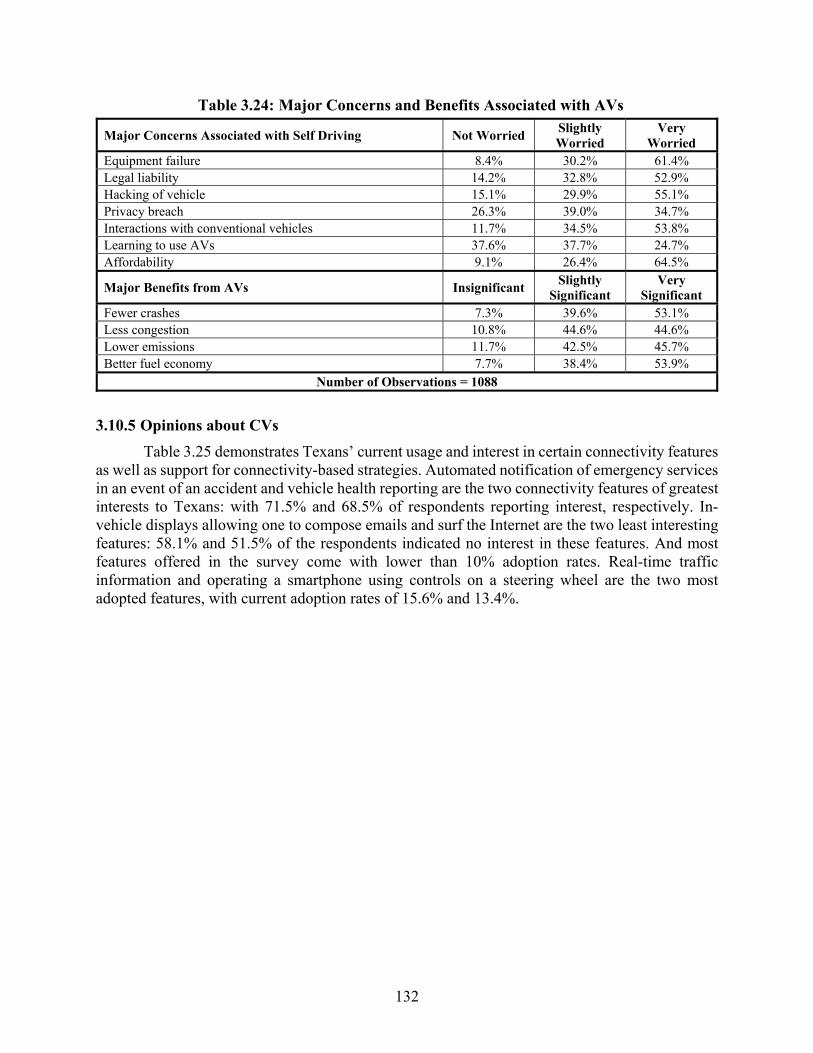
132

Table 3.24: Major Concerns and Benefits Associated with AVs

Major Concerns Associated with Self Driving Not Worried Slightly Worried

Very Worried

Equipment failure 8.4% 30.2% 61.4% Legal liability 14.2% 32.8% 52.9% Hacking of vehicle 15.1% 29.9% 55.1% Privacy breach 26.3% 39.0% 34.7% Interactions with conventional vehicles 11.7% 34.5% 53.8% Learning to use AVs 37.6% 37.7% 24.7% Affordability 9.1% 26.4% 64.5%

Major Benefits from AVs Insignificant Slightly

Significant Very

Significant Fewer crashes 7.3% 39.6% 53.1% Less congestion 10.8% 44.6% 44.6% Lower emissions 11.7% 42.5% 45.7% Better fuel economy 7.7% 38.4% 53.9%

Number of Observations = 1088

3.10.5 Opinions about CVs

Table 3.25 demonstrates Texans’ current usage and interest in certain connectivity features as well as support for connectivity-based strategies. Automated notification of emergency services in an event of an accident and vehicle health reporting are the two connectivity features of greatest interests to Texans: with 71.5% and 68.5% of respondents reporting interest, respectively. In-vehicle displays allowing one to compose emails and surf the Internet are the two least interesting features: 58.1% and 51.5% of the respondents indicated no interest in these features. And most features offered in the survey come with lower than 10% adoption rates. Real-time traffic information and operating a smartphone using controls on a steering wheel are the two most adopted features, with current adoption rates of 15.6% and 13.4%.

133

Table 3.25: Current Adoption and Interest in Connectivity Features

Not Interested

Interested Already Using

Real-time traffic information 22.6% 61.8% 15.6% Alert about the presence of roadside speed cameras 27.6% 65.6% 6.7% Information about nearby available parking 33.6% 61.7% 4.7% Automatic notification to emergency personnel in the event of an accident 18.8% 71.5% 9.7% Automatic monitoring of driving habits by insurance companies 49.6% 44.2% 6.2% Personal restrictions (example: certain speed limits for teenagers) 38.4% 53.8% 7.8% Alcohol detection 38.0% 53.8% 8.2% Road sign information 37.4% 58.1% 4.5% Cabin pre-conditioning 27.3% 65.6% 7.1% Vehicle health report 19.3% 68.5% 12.2% Vehicle life-cycle management 23.2% 63.5% 13.3% Surfing the Internet via a built-in car display 51.5% 43.2% 5.2% In-vehicle feature allowing to use email 58.1% 38.3% 3.6% Operating a smartphone using controls on the steering wheel 38.5% 48.1% 13.4%

Number of Observations = 1063 The questions about interest in connectivity features were only asked to the respondents (1,063 out of 1,088

respondents) who either have at least a vehicle or are planning to buy a vehicle in the next 5 years

Table 3.26 suggests that Texans appear likely to support adaptive traffic signal timing and

but unlikely to support real-time adjustment in parking prices (when 80% of vehicles are connected): 64.0% and 20.5% of respondents reported support for these policies, respectively. On average, Texans ranked safety as the most important and climate change as the least important area of improvement in automobile technologies.

Table 3.26: Support for CV-related Strategies and Improvements in Automobile Technologies

Do Not Support

No Opinion

Support

Adaptive traffic signal timing to ease congestion 13.0% 23.1% 64.0%Real-time adjustment of parking prices 48.5% 31.0% 20.5%Variable toll rates on congested corridors 37.3% 29.2% 33.5%Variable speed limits based on road and weather conditions 18.3% 19.5% 62.2%Areas of Improvement Average RankSafety 1.36 Emissions (excluding greenhouse gas) 2.27 Travel times (and congestion) 2.64 Energy use and climate change 2.67

Number of Observations = 1088

3.10.6 Opinions about Carsharing and Transportation Network Companies

Table 3.27 shows that, among those who have heard about carsharing, only 10% are members of carsharing programs (e.g., Zipcar or Car2Go). These members indicated that

134

environmental friendliness and monetary savings are the two key reasons behind the joining the programs. Among non-member respondents, most (75.5%) find no current reason to join a carsharing program because they rely on other means of transportation. Among those who have heard about UberX or Lyft, only 12.2% have used such services as a passenger. According to these users, cost and time savings are their primary reasons for using such services. Lastly, only 16.4% of Texans are comfortable in sharing a ride with a complete stranger.

Table 3.27: Opinions about Carsharing and On-demand Taxi Services

Carsharing (Zipcar, Gar2Go)

Heard about carsharing 25.5%

Among those who have heard about carsharing: Member of Zipcar or Car2Go 9.9% Not a member 90.1%

Why a member? (Among members) Why not a member? (Among non-members) Saves money 68.2% Not available where I live 25.9% Saves time 60.0% Inconvenient availability or location 21.6% Environmentally friendly 68.7% Own a vehicle, use transit, or walk 75.5% Necessity (I have no car) 38.6% It is expensive 10.3% Good back up 35.9% Not ready to share a vehicle 27.6% Other 5.2% Other 18.2%

On-demand Taxi Service (UberX or Lyft)

Heard about UberX or Lyft 64.0%

Among those who heard about UberX or Lyft

Used UberX as a Passenger 12.2%

With Whom Will be Comfortable Sharing a Ride With a stranger 16.4% With close friends and family 75.9% With a friend of a friend 39.9% Other 2.6% With regular friends and family 45.4%

Among those who Have Used UberX as Passengers

Why Used UberX To save money 54.4% No need to worry about parking 21.4% To save time 47.0% My vehicle was unavailable 16.9% To try it out 43.3% Promotion 24.1% To avoid driving 41.6% Other 4.0%

Number of Observations = 1088

3.11 Model Estimation

This study estimated WTP to add connectivity and different levels of automation using an IR model57. Wooldridge (2013) provides many details about the IR model, which is succinctly presented here for interval response values58. The key equation is as follows:

57 Respondents were asked to choose WTP interval (e.g., $1,500 to $2,999 to add automation) and also provided with options of “$3,000 or more” and “$1,000 or more” in the questions about WTP to add automation and connectivity, respectively. Thus, the response variable is right-censored interval data. IR is an extension of linear regression and reflects all interval boundaries as known values, unlike an OP or logit model specification. 58 IR can be used to model point, interval, right-censored, and left-censored data types.

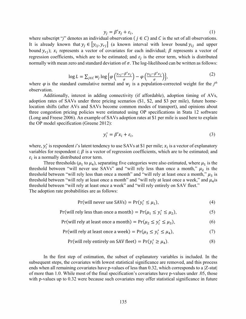
135

= ′ + , (1)where subscript “j” denotes an individual observation ( ∈ ) and is the set of all observations. It is already known that ∈ , (a known interval with lower bound and upper bound ); represents a vector of covariates for each individual; represents a vector of regression coefficients, which are to be estimated; and is the error term, which is distributed normally with mean zero and standard deviation of . The log-likelihood can be written as follows:

log = ∑ log −∈ , (2)

where is the standard cumulative normal and is a population-corrected weight for the jth observation.

Additionally, interest in adding connectivity (if affordable), adoption timing of AVs, adoption rates of SAVs under three pricing scenarios ($1, $2, and $3 per mile), future home-location shifts (after AVs and SAVs become common modes of transport), and opinions about three congestion pricing policies were estimated using OP specifications in Stata 12 software (Long and Freese 2006). An example of SAVs adoption rates at $1 per mile is used here to explain the OP model specification (Greene 2012): ∗ = ′ + , (3) where, ∗ is respondent i’s latent tendency to use SAVs at $1 per mile; is a vector of explanatory variables for respondent i; is a vector of regression coefficients, which are to be estimated; and

is a normally distributed error term. Three thresholds ( to ), separating five categories were also estimated, where is the

threshold between “will never use SAVs” and “will rely less than once a month,” is the threshold between “will rely less than once a month” and “will rely at least once a month,” is threshold between “will rely at least once a month” and “will rely at least once a week,” and is threshold between “will rely at least once a week” and “will rely entirely on SAV fleet.” The adoption rate probabilities are as follows: Pr(willnever use SAVs) = Pr( ∗ ≤ ), (4)Pr(will relylessthan once a month) = Pr( ≤ ∗ ≤ ), (5)Pr(willrelyatleast once a month) = Pr( ≤ ∗ ≤ ), (6)Pr(willrelyatleast once a week) = Pr( ≤ ∗ ≤ ), (7)Pr(willrelyentirely on SAV fleet) = Pr( ∗ ≥ ). (8)

In the first step of estimation, the subset of explanatory variables is included. In the

subsequent steps, the covariates with lowest statistical significance are removed, and this process ends when all remaining covariates have p-values of less than 0.32, which corresponds to a |Z-stat| of more than 1.0. While most of the final specification’s covariates have p-values under .05, those with p-values up to 0.32 were because such covariates may offer statistical significance in future

136

studies. They do not have high collinearity with other covariates, so it is valuable to get a sense of their practical significance, even if they lack some statistical significance in this data set.

Apart from statistical significance, practical significance is important to understand the strength of relationship or correlation between covariates and response variables. It was measured based on the change in response values due to a one-standard-deviation (SD) rise in each covariate. In the IR models for WTP, covariates with standardized coefficients greater than 0.2 (i.e., those offering a 0.2 standard deviation change in WTP due to 1 SD change in the covariate) are considered practically significant. In the OP model, the choice probabilities are the response variables, so covariates were considered practically significant if the associated probabilities shift by 40% or more (i.e., to 1.4 or 0.6 of their original predictions). Finally, R-square and adjusted R-square values are provided as the goodness of fit indicators.

3.11.1 Interest in and WTP to add Connectivity

Tables 3.28 and 3.29 summarize the OP and IR model estimates of Texans’ interest in and WTP for adding connectivity to their vehicles, respectively. These results indicate that more experienced licensed drivers and single individuals are less interested in adding connectivity and have lower WTP for it. Men who are familiar with carsharing, support speed regulation strategies, carry smartphones, drive alone for work, make more social/recreational trips, live further away from downtown, and enjoy higher household income (everything else constant) are estimated to have more interest in adding connectivity (if it is affordable), while those living farther from transit stops appear less interested.

Men with disabilities and with bachelor’s degrees, who are familiar with TNC’s services, travel more, make more business trips, support speed governors, and have experienced more moving violations and/or fatal crashes in the past (all other predictors constant) are estimated to have higher WTP for adding connectivity, while older Caucasians with more household members are estimated to place lower value on connectivity. Perhaps the educated, safety-seeking, and tech-savvy respondents are able to perceive the safety benefits of connectivity during their longer travels.

137

Table 3.28: Interest in Connectivity Model Results (using OP)

Covariates Coef. Z-stat ΔPr1 ΔPr2 ΔPr3

Licensed driver (number of years) -0.032 -4.98 46.1% 2.5% -28.7%Support the use of Automated Speed Enforcement? 0.483 3.7 -23.9% -5.1% 20.2% Support the use of Speed Governors on all new vehicles? 0.555 4.12 -27.0% -6.1% 23.1% Number of fatal (or serious) crashes in past 15 years 0.407 2.08 -50.6% -16.2% 50.0% Carry smartphone? 0.541 3 -20.5% -4.2% 17.0% Familiar with carsharing? 0.418 2.95 -19.2% -3.9% 15.8% Drive alone for work trips? 0.25 1.91 -12.8% -2.3% 10.2% More than 2 social (or recreational) trips in past 7 days 0.234 1.82 -11.2% -2.0% 8.9% Distance between home and public transit stop (miles) -0.02 -2.02 13.9% 1.6% -9.8% Home and city’s downtown are more than 10 miles apart? 0.17 1.35 -8.9% -1.5% 7.0% Male? 0.298 2.24 -15.2% -2.9% 12.3% Household income ($) 2.36E-06 1.75 -11.6% -2.1% 9.2% Single? -0.351 -2.25 18.4% 1.9% -12.7% Thresholds Coef. Std. Dev. Not interested vs. Neutral -0.356 0.282 -- -- --Neutral vs. Interested 1.368 0.285 -- -- --

Nobs: 1063 McFadden’s R-Square: 0.082 McFadden’s adjusted R-Square: 0.070 Note: All ΔPr’s, which are greater than 40%, are in bold, and indicate practically significant predictors. All results are population weighted/sample corrected.

Table 3.29: WTP for Connectivity Model Results (using IR)

Covariates Coef. Std. Coef. Z-statIntercept 151.40 -- 4.64Number of moving violations in past 10 years 10.01 0.129 5.96 Support the use of Speed Governors on all new vehicles? 48.37 0.148 5.04 Number of fatal (or serious) crashes in past 15 years 6.69 0.034 1.95 Number of crashes with only monetary loss in past 15 years 3.79 0.073 1.45 Familiar with UberX or Lyft? 21.03 0.060 2.04 Licensed driver (number of years) -2.48 -0.216 -3.24 Number of personal business trips in past 7 days 4.48 0.053 2.27 Annual VMT (miles) 1.95E-03 0.068 2.44 No disability? -17.89 -0.041 -1.23 Household size -7.20 -0.073 -1.90 Age of Respondent (years) -0.99 -0.077 -1.74 Male? 10.32 0.042 1.11 White, European white or Caucasian? -19.66 -0.062 -1.98 Household income ($) 5.96E-04 0.172 7.16 Bachelor’s degree holder 15.03 0.035 1.52 Single? -17.22 -0.058 -1.48 sigma 138.30 -- --

Nobs: 1063 McFadden’s R-Square: 0.038 McFadden’s adjusted R-Square: 0.034 Note: All Std. Coef., which are greater than 0.2, are in bold, and indicate practically significant predictors. All results are population weighted/sample corrected.

3.11.2 WTP for Automation Technologies

Table 3.30 summarizes the IR model specifications of WTP to add Level 2, Level 3, and Level 4 automation. As expected, intercepts in these models rise along with automation level. Respondents who have heard about the Google self-driving car (before taking the survey), support

138

speed governors on all new vehicles, and have higher household income (everything else constant) are estimated to pay more for all levels of automation. However, consistent with the findings of the WTP for Connectivity model results, older and more experienced licensed drivers are expected to place lower value on automation technologies. Perhaps older individuals are finding it difficult to conceive that CAVs are about to hit the roads and licensed drivers who particularly enjoy driving might be worried about sacrificing those elements of driving they find enjoyable.

Individuals with higher annual VMT appear willing to pay more for Level 4 automation, but that preference is inverted for those living in more densely populated neighborhoods. Those who live farther from transit stops are found less willing to pay for Level 3 and Level 4 automation. Caucasians’ WTP for Level 2 automation is estimated to be lower than that for other ethnicities, as is the case for connectivity, implying that non-Caucasians may be early adopters of CAV technologies. Interestingly, those who experienced more fatal crashes in the past appear significantly interested in paying more for Level 2 and Level 3 automation (as is the case for connectivity); surprisingly, this relationship reverses for those who are familiar with TNC’s services.

139

Table 3.30: WTP for Automation Technologies Model Results (using IR)

Covariates (Model 1: WTP for Level 4 Automation) Coef. Std. Coef. Z-statIntercept 10300 -- 7.43Have heard about Google car? 1521 0.099 2.64 Support the use of Speed Governors on all new vehicles? 1755 0.120 3.32 Have heard about CVs? 931.1 0.054 1.28 Licensed driver (number of years) -61.07 -0.092 -1.27 Distance between home and public transit stop (miles) -75.18 -0.061 -1.60 Annual VMT (miles) 9.96E-02 0.078 2.40 Age of Respondent (years) -104.60 -0.229 -2.71 Household income ($) 1.04E-02 0.078 1.81 Single? 1000 0.064 1.63 Population density (per square mile) -0.11 -0.046 -1.29 Sigma (σ) 6961 -- --Nobs: 755 McFadden’s R-Square: 0.035 McFadden’s adjusted R-Square: 0.029

Covariates (Model 2: WTP for Level 3 Automation) Coef. Std. Coef. Z-statIntercept 7179 -- 7.17Have heard about Google car? 1094 0.099 2.58 Support the use of Speed Governors on all new vehicles? 1229 0.114 3.27 Number of fatal (or serious) crashes in past 15 years 438.6 0.134 4.82 Familiar with UberX or Lyft? -506.8 -0.041 -1.21 Licensed driver (number of years) -54.56 -0.118 -1.52 Number of personal business trips in past 7 days 96.91 0.037 1.06 Distance between home and public transit stop (miles) -42.49 -0.049 -1.26 Distance between home and city’s downtown (miles) 40.98 0.045 1.22 Age of Respondent (years) -73.12 -0.217 -2.45 Household income ($) 7.53E-03 0.069 1.79 Sigma (σ) 4792 -- --Nobs: 755 McFadden’s R-Square: 0.044 McFadden’s adjusted R-Square: 0.039

Covariates (Model 3: WTP for Level 2 Automation) Coef. Std. Coef. Z-statIntercept 5059 -- 6.65Have heard about Google car? 896.8 0.101 2.45 Support the use of Speed Governors on all new vehicles? 1241 0.144 3.94 Number of fatal (or serious) crashes in past 15 years 554.6 0.212 8.36 Familiar with UberX or Lyft? -750.7 -0.076 -2.24 Licensed driver (number of years) -51.35 -0.140 -1.80 Household size over 3? -501.4 -0.053 -1.57 Age of Respondent (years) -38.91 -0.245 -1.63 White, European white or Caucasian? -467.8 -0.052 -1.39 Household income ($) 5.55E-03 0.064 1.69 Sigma (σ) 3743 -- --Nobs: 755 McFadden’s R-Square: 0.048 McFadden’s adjusted R-Square: 0.042 Note: All Std. Coef., which are greater than 0.2, are in bold, and indicate practically significant predictors. All results are population weighted/sample corrected.

3.11.3 Adoption Timing of Autonomous Vehicles

Table 3.31 summarizes OP model estimates of AV adoption timings (i.e., will never adopt an AV, will adopt AVs when 50% of friends adopt, when 10 % of friends adopt, or as soon as available in the market). The adoption timing of disabled individuals and bachelor’s degree holders

140

who support speed-regulation strategies, are familiar with carsharing, travel more, have more than one worker in the household, and live in a neighborhood with a higher density of employed individuals—all other predictors constant—are less likely to depend on friends’ adoption rates. In contrast, the adoption timing of older, single, and Caucasian respondents who have larger households and live farther from bus stop in more densely populated neighborhoods is estimated to be more dependent on friends’ adoption rates. These estimates appear to be consistent with the WTP for Automation Technologies model results59. In other words, the AV adoption timing of those who indicate higher WTP for AVs is less likely to depend on their friends’ adoption rates.

Table 3.31: Adoption Timing of AVs Model Results (using OP)

Covariates Coef. Z- ΔPr1 ΔPr2 ΔPr3 ΔPr4

Support the use of Automated Speed Enforcement? 0.455 1.82 - 3.6% 23.3% 43.0%Support the use of Speed Governors on all new vehicles? 0.365 1.99 - 3.1% 18.5% 33.3% Have heard about CVs? 0.362 1.52 - 2.5% 13.9% 24.4% Familiar with carsharing? 0.336 2.19 - 2.8% 15.6% 27.6% Distance between home and public transit stop (miles) -0.051 -2.44 26.1% -9.3% - -41.9%Annual VMT (miles) 3.13E-05 1.74 - 3.3% 20.1% 36.4% No disability? -0.454 -1.65 11.8% -3.7% - -21.5% Household size -0.109 -1.69 12.4% -3.9% - -22.5% More than 1 worker in household? 0.259 1.41 - 2.4% 12.9% 22.6% Age of Respondent (years) -0.025 -2.53 33.9% - - -51.0%White, European white or Caucasian? -0.273 -1.32 10.6% -3.3% - -19.4% Bachelor’s degree holder 0.260 1.50 - 2.4% 12.9% 22.6% Single? -0.385 -1.83 14.5% -4.7% - -25.8% Population density (per square mile) -1.76E-04 -1.47 48.8% - - -65.0%Employed and over 16 years of age (per square mile) 1.96E-04 1.09 - 24.2% 22.7% 33.3% Thresholds Coef. Std. Never vs. 50% friends adopt -1.898 0.665 -- -- -- --50% friends adopt vs. 10% friends adopt -0.303 0.688 -- -- -- -- 10% friends adopt vs. As soon as available 0.555 0.738 -- -- -- -- Nobs: 1,088 McFadden’s R-Square: 0.059 McFadden’s adjusted R-Square: 0.046Note: All ΔPr’s greater than 40% are in bold, and indicate practically significant predictors. All results are population weighted/sample corrected.

3.11.4 SAV Adoptions Rates under Different Pricing Scenarios

Table 3.32 summarizes the OP model estimates of SAV adoption rates (i.e., relying on an SAV fleet less than once a month, at least once a month, at least once a week, or entirely) under different pricing scenarios ($1 per mile [Model 1], $2 per mile [Model 2], and $3 per mile [Model 3]). Respondents who experienced fatal crashes in the past, support speed regulation strategies, have heard about CVs, live farther from downtown, and have more workers in households, all other predictors constant, are likely to use SAVs frequently. In contrast, consistent with WTP for automation technologies model findings, Caucasians who are licensed (or more experienced)

59 As an exception, single respondents are estimated to have higher WTP to add Level 4 automation (other attributes held constant), but their adoption timing depends more on their friends’ adoption rates.

141

drivers and live farther from transit stops are estimated to use SAVs less frequently in all three pricing scenarios60.

It is worth noting that even unemployed and lower income households (with annual household income less than $30,000) are estimated to use SAVs more frequently at $1 per mile; perhaps SAVs are affordable for these individuals at this price. Male respondents who travel more also expect to use SAVs more frequently at $1 per mile, since they can readily evaluate cost-reduction benefits at this lower price. Respondents who have experienced more moving violations in the past are expected to use SAVs frequently at $1 and $2 per mile; perhaps they can visualize that SAVs can save them from future violations61. Interestingly, married respondents who are familiar with UberX (everything else constant) are estimated to use SAVs less frequently, but those who make more social/recreation trips are expected to use SAVs frequently at even $2 and $3 per mile (more than what carsharing companies and UberX charge). Perhaps those who know about TNC’s services are not willing to pay additional charges to enjoy SAVs’ additional utilities; the vehicle ownership level (not controlled here) of married couples might be discouraging them from using SAVs at higher prices. Lastly, perhaps bigger households are likely to use SAVs as an alternative to a second vehicle and disabled individuals are able to perceive the maximum utility of SAVs, and thus both demographic groups are likely to use SAVs more frequently, even at $3 per mile.

60 Since household vehicle ownership is not controlled here, the respondents showing negative inclination towards SAVs may have higher vehicle ownership, on average. 61 However, even respondents who experienced more moving violations in the past do not attach statistical significance to the SAVs’ utility of saving them from future violations at $3 per mile.

142

Table 3.32: SAV Adoption Rates under Different Pricing Scenarios Model Results (using OP)

Covariates (Model 1: $1 per mile) Coef. Z-stat ΔPr1 ΔPr2 ΔPr3 ΔPr4 ΔPr5

Number of moving violations in past 10 years 0.081 1.91 -32.3% -16.7% -4.8% 8.0% 20.6%

Support the use of Automated Speed Enforcement? 0.407 2.11 -32.3% -16.7% -4.7% 8.0% 20.5%

Support the use of Speed Governors on all new vehicles? 1.040 5.49 -65.4% -40.3% -15.0% 18.4% 59.7%

At least 1 fatal (or serious) crash in past 15 years? 0.615 1.64 -29.2% -14.9% -4.2% 7.1% 18.1%

Have heard about CVs? 0.501 1.64 -30.9% -15.9% -4.5% 7.6% 19.5%

Distance between home and public transit stop (miles) -0.038 -2.15 47.8% 19.0% 3.3% -9.3% -18.9%

Distance between home and city’s downtown (miles) 0.025 1.66 -24.9% -12.5% -3.4% 6.0% 14.9%

Annual VMT more than 15,000 miles? 0.298 1.35 -20.2% -9.9% -2.6% 4.8% 11.7%

Number of workers in household 0.227 2.34 -34.5% -18.0% -5.2% 8.6% 22.4%

Male? -0.257 -1.29 26.4% 11.2% 2.2% -5.5% -11.5%

Have U.S. driver license? -1.163 -3.15 72.7% 27.2% 4.2% -13.4% -25.9%

White, European white or Caucasian? -0.419 -2.13 45.0% 18.0% 3.2% -8.8% -18.0%

Household income less than $30,000? 0.425 2.11 -30.4% -15.6% -4.4% 7.5% 19.0%

Unemployed? 0.508 2.10 -31.4% -16.2% -4.6% 7.7% 19.8%

Thresholds Coef. Std. Dev.

Never use vs. Rely less than once a month -2.510 0.431 -- -- -- -- --

Rely less than once a month vs. Rely at least once a month -0.769 0.412 -- -- -- -- --

Rely at least once a month vs. Rely at least once a week 0.510 0.411 -- -- -- -- --

Rely at least once a week vs. Rely entirely on SAV fleet 2.409 0.455 -- -- -- -- --

Nobs: 730 McFadden’s R-Square: 0.113 McFadden’s adjusted R-Square: 0.097

143

Table 3.32, continued Covariates (Model 2: $2 per mile) Coef. Z-stat ΔPr1 ΔPr2 ΔPr3 ΔPr4 ΔPr5

Licensed driver (number of years) -0.017 -1.60 22.8% 6.7% -2.3% -14.1% -21.2%

Number of moving violations in past 10 years 0.093 1.90 -22.4% -8.6% 0.9% 16.3% 31.5%

Support the use of Automated Speed Enforcement? 0.515 2.40 -24.5% -9.5% 0.9% 17.9% 35.1%

Support the use of Speed Governors on all new vehicles? 0.899 4.02 -40.3% -17.4% 0.2% 31.2% 70.1%

Number of fatal (or serious) crashes in past 15 years 0.179 1.62 -28.1% -11.2% 0.8% 20.8% 42.1%

Have heard about CVs? 0.640 2.47 -23.6% -9.1% 0.9% 17.2% 33.5%

Familiar with UberX or Lyft? -0.527 -2.24 26.8% 7.6% -2.8% -16.3% -24.1%

Drive alone for work trips? -0.330 -1.61 17.8% 5.4% -1.7% -11.2% -17.2%

More than 2 social (or recreational) trips in past 7 days 0.401 1.95 -18.8% -7.0% 0.9% 13.5% 25.4%

Distance between home and public transit stop (miles) -0.057 -2.90 37.6% 10.1% -4.3% -22.1% -31.3%

Distance between home and city’s downtown (miles) 0.036 2.17 -20.9% -7.9% 0.9% 15.1% 28.9%

Number of workers in household 0.277 2.21 -25.4% -9.9% 0.9% 18.6% 36.9%

Older than 54 years? -0.498 -2.05 25.6% 7.4% -2.7% -15.7% -23.3%

White, European white or Caucasian? -0.379 -1.92 20.7% 6.1% -2.0% -12.9% -19.5%

Married? -0.383 -1.98 21.4% 6.3% -2.1% -13.3% -20.1%

Thresholds Coef. Std. Dev.

Never use vs. Rely less than once a month -1.435 0.443 -- -- -- -- --

Rely less than once a month vs. Rely at least once a month 0.040 0.429 -- -- -- -- --

Rely at least once a month vs. Rely at least once a week 1.302 0.444 -- -- -- -- --

Rely at least once a week vs. Rely entirely on SAV fleet 3.191 0.536 -- -- -- -- --

Nobs: 730 McFadden’s R-Square: 0.123 McFadden’s adjusted R-Square: 0.108

144

Table 3.32, continued Covariates (Model 3: $3 per mile) Coef. Z-stat ΔPr1 ΔPr2 ΔPr3 ΔPr4 ΔPr5

Licensed driver (number of years) -0.018 -2.28 16.1% 1.7% -7.4% -19.2% -24.9%

Support the use of Automated Speed Enforcement? 0.475 2.37 -16.4% -3.4% 6.5% 23.3% 36.8%

Support the use of Speed Governors on all new vehicles? 0.895 4.34 -30.1% -7.7% 10.7% 46.0% 81.8%

Number of fatal (or serious) crashes in past 15 years 0.191 3.61 -21.8% -4.9% 8.3% 31.9% 52.7%

Have heard about CVs? 0.874 3.03 -22.9% -5.3% 13.6% 33.7% 36.2%

Familiar with UberX or Lyft? -0.259 -1.38 8.6% 1.1% -3.8% -10.6% -14.4%

Number of social (or recreational) trips in past 7 days 0.080 1.68 -11.0% -2.1% 4.5% 15.1% 23.1%

Distance between home and public transit stop (miles) -0.056 -3.01 24.1% 2.0% -11.4% -27.5% -34.5%

Distance between home and city’s downtown (miles) 0.032 1.86 -13.4% -2.6% 5.4% 18.8% 29.1%

No disability? -0.495 -1.72 12.2% 1.4% -5.5% -14.8% -19.6%

Household size over 3? 0.291 1.49 -9.6% -1.8% 3.9% 13.1% 19.7%

Number of workers in household 0.127 1.17 -8.7% -1.6% 3.6% 11.8% 17.7%

White, European white or Caucasian? -0.661 -3.40 24.5% 2.0% -11.6% -27.9% -34.9%

Married? -0.452 -2.33 16.9% 1.7% -7.8% -20.0% -26.0%

Thresholds Coef. Std. Dev.

Never use vs. Rely less than once a month -0.828 0.475 -- -- -- -- --

Rely less than once a month vs. Rely at least once a month 0.326 0.479 -- -- -- -- --

Rely at least once a month vs. Rely at least once a week 1.632 0.490 -- -- -- -- --

Rely at least once a week vs. Rely entirely on SAV fleet 3.381 0.606 -- -- -- -- --

Nobs: 730 McFadden’s R-Square: 0.121 McFadden’s adjusted R-Square: 0.105

Note: The respondents were first asked about their SAV adoption rates if the SAV service were affordable. Those who never want to use SAVs (358 out of 1088 respondents), even if they are affordable, were not asked the questions about SAVs’ adoption rates under different pricing scenarios. All ΔPr’s, which are greater than 40%, are in bold, and indicate practically significant predictors. All results are population weighted/sample corrected.

145

3.11.5 Home Location Shifts due to AVs and SAVs

Table 3.33 summarizes the OP model estimates of respondents’ home-location-shift decisions (i.e., shift closer to central Austin, stay at the same location, or move farther from central Austin)62 after AVs and SAVs become common modes of transport. Bachelor’s degree holders, single individuals, and full-time workers who support speed governors, own at least a vehicle with Level 2 automation, have experienced more fatal crashes in past, and live farther from a city center—all other attributes constant—are likely to shift closer to the city center. Perhaps these individuals are excited about higher density of low-cost SAVs near city center. However, respondents who live farther from transit stops, make more social/recreation trips, and are familiar with UberX (everything else constant) are predicted to shift farther from the city center. Perhaps these individuals are concerned about higher land prices in the urban neighborhoods, and are keen to enjoy the benefits of moving to suburban areas after AVs and SAVs become common modes of transport.

Table 3.33: Home Location Shifts due to AVs and SAVs Model Results (using OP)

Covariates Coef. Z-stat ΔPr1 ΔPr2 ΔPr3

Own a vehicle? -1.386 -3.25 28.9% -1.6% -34.7%Own at least a vehicle with Level 2 automation? -1.443 -3.22 72.6% -0.8% -39.7% Support the use of Speed Governors on all new vehicles? -0.466 -2.06 39.1% -0.3% -26.4% Number of fatal (or serious) crashes in past 15 years -0.170 -1.75 32.4% -0.6% -27.6% Familiar with UberX or Lyft? 0.336 1.44 -21.0% -0.2% 23.0% Distance from city centre (miles) -0.068 -3.65 79.0% -0.9% -41.8% Drive alone for work trips? 0.291 1.20 -19.5% -0.2% 20.9% Number of social (or recreational) trips in past 7 days 0.069 1.38 -18.1% -0.2% 19.1% Distance between home and public transit stop (miles) 0.049 2.59 -37.2% -0.7% 49.1% Older than 54 years? -0.464 -2.17 38.2% -0.2% -25.5% Male? -0.428 -2.03 36.4% -0.2% -24.6% White, European white or Caucasian? -0.349 -1.37 27.4% -0.1% -19.7% Bachelor’s degree holder -0.263 -1.32 20.8% -0.1% -15.7% Full time worker? -0.445 -1.65 36.9% -0.2% -24.9% Single? -0.431 -1.63 33.6% -0.2% -23.2% Thresholds Coef. Std. Shift closer vs. stay at the same location -4.992 0.589 -- -- --stay at the same location vs. shift farther 0.103 0.518 -- -- -- Nobs: 1088 McFadden’s R-Square: 0.112 McFadden’s adjusted R-Square: 0.087

Note: All ΔPr’s, which are greater than 40%, are in bold, and indicate practically significant predictors. All results are population weighted/sample corrected.

62 This model alone can obtain inferences about two groups’ characteristics: those “who want to shift closer to the city center or stay at the same location” and those “who want to shift farther from the city center or stay at the same location.” However, to explore the characteristics of population groups “who want to shift closer to the city center” and “who want to shift farther from the city center,” a new binary logit model was estimated so as to explore the individual characteristics of those “who want to stay at the same location” after AVs and SAVs become common modes of transport. For example, according to OP model estimates, those who are familiar with UberX are either likely to shift farther from the city center or stay at the same location, but the binary logit model suggests that these individuals are likely to shift. This new binary logit model clarifies that these individuals are expected to shift farther from the city center.

146

3.11.6 Support for Tolling Policies

Table 3.34 summarizes the OP model estimates of respondents’ opinions (i.e., definitely not support, probably not support, do not know, probably support, or definitely support) about three tolling policies63. In Policy 1, revenue from tolled congested highways is used to reduce property taxes; in Policy 2, revenue from tolled congested highways is distributed evenly among Texans; in Policy 3, time varying tolls are enabled on all congested roadways. Results indicate that Caucasians who are licensed (or more experienced) drivers and live farther from transit stops, everything else constant, are likely to show refusal for all tolling policies. Perhaps these individuals are concerned that they would be the primary toll payers64, and only others would benefit from these three policies. Interestingly, bachelor’s degree holders who live farther from downtown are estimated to support Policies 1 and 2; full-time workers who have more children in the household are likely to support Policies 2 and 3. Older respondents are predicted to refuse the options presented by Policies 1 and 3. Respondents whose households own at least one vehicle and live in populous areas (everything else constant) specifically showed refusal for Policy 3, but those who live in neighborhoods with more employed individuals are likely to support this policy.

63 Safety- and tech-based predictors were not used in these models’ specifications. 64 However, individuals who travel more, all other attributes remaining equal, are likely to support tolling policies 2 and 3.

147

Table 3.34: Support for Tolling Policies Model Results (using OP)

Covariates (Model 1: Toll Congested Highways if Reduce Property Tax)

Coef. Z-stat ΔPr1 ΔPr2 ΔPr3 ΔPr4 ΔPr5

Licensed driver for more than 20 years? -0.462 -2.21 27.8% 11.1% -0.9% -16.3% -32.2%More than 2 social (or recreational) trips in past 7 days 0.295 1.69 -14.7% -7.5% -0.9% 9.5% 24.2% Distance between home and public transit stop (miles) -0.041 -2.53 31.1% 12.2% -1.2% -18.1% -35.3% Distance between home and city’s downtown (miles) 0.030 2.09 -19.1% -10.0% -1.4% 12.4% 32.7% Household size over 3? -0.300 -1.50 16.0% 6.8% -0.2% -9.6% -20.2% Number of workers in household 0.228 2.27 -22.6% -12.0% -1.9% 14.8% 40.1% Older than 54 years? -0.474 -1.91 27.6% 11.0% -0.9% -16.2% -32.1% White, European white or Caucasian? -0.553 -2.37 32.3% 12.5% -1.3% -18.7% -36.2% Bachelor’s degree holder 0.365 2.33 -19.0% -9.9% -1.4% 12.3% 32.5% Thresholds Coef. Std. Definitely not support vs. Probably not support -1.372 0.331 -- -- -- -- --Probably not support vs. Do not know -0.886 0.321 -- -- -- -- -- Do not know vs. Probably Support 0.268 0.325 -- -- -- -- -- Probably support vs. Definitely support 1.548 0.345 -- -- -- -- -- Nobs: 1,088 McFadden’s R-Square: 0.049 McFadden’s adjusted R-Square: 0.041

Covariates (Model 2: Toll Congested Highways if Distribute Revenues)

Coef. Z-stat ΔPr1 ΔPr2 ΔPr3 ΔPr4 ΔPr5

Licensed driver (number of years) -0.043 -5.74 62.6% 15.2% -8.7% -36.7% -63.6%Distance between home and public transit stop (miles) -0.051 -4.00 36.9% 10.8% -4.0% -23.1% -45.2% Distance between home and city’s downtown (miles) 0.026 1.83 -15.9% -6.8% 0.2% 11.5% 31.1% Annual VMT (miles) 2.63E-05 2.00 -16.7% -7.2% 0.1% 12.1% 33.1% White, European white or Caucasian? -0.460 -2.93 24.8% 7.9% -2.2% -16.1% -33.5% Number of children in household 0.160 2.05 -17.0% -7.3% 0.1% 12.3% 33.7% Bachelor’s degree holder 0.227 1.50 -11.5% -4.7% 0.2% 8.2% 21.5% Full time worker? 0.307 1.89 -15.2% -6.4% 0.2% 10.9% 29.5% Thresholds Coef. Std. Definitely not support vs. Probably not support -1.780 0.280 -- -- -- -- --Probably not support vs. Do not know -1.086 0.272 -- -- -- -- -- Do not know vs. Probably Support 0.027 0.272 -- -- -- -- -- Probably support vs. Definitely support 1.596 0.251 -- -- -- -- -- Nobs: 1,088 McFadden’s R-Square: 0.061 McFadden’s adjusted R-Square: 0.054

148

Table 3.34, continued

Covariates (Model 3: Time-varying tolls on All Congested Roadways)

Coef. Z-stat ΔPr1 ΔPr2 ΔPr3 ΔPr4 ΔPr5

Own a vehicle? -0.754 -1.35 23.5% 10.2% -0.7% -13.7% -27.7%More than 2 personal business trips in past 7 days? 0.293 1.14 -14.1% -7.3% -0.4% 9.4% 22.9% Distance between home and public transit stop (miles) -0.024 -1.44 19.8% 8.7% -0.5% -11.7% -24.0% Annual VMT (miles) 1.92E-05 1.48 -14.4% -7.5% -0.4% 9.6% 23.6% Age of Respondent (years) -0.015 -1.84 33.8% 13.9% -1.4% -19.0% -36.8% Have U.S. driver license? 0.342 1.00 -10.6% -5.4% -0.2% 6.9% 16.7% White, European white or Caucasian? -0.903 -4.33 62.8% 22.7% -4.3% -32.4% -56.4% Number of children in household 0.168 1.91 -20.6% -11.1% -0.9% 14.0% 35.8% Full time worker? 0.265 1.66 -15.3% -8.0% -0.5% 10.2% 25.3% Population density (per square mile) -2.51E-04 -1.41 36.7% 34.6% -15.6% -57.7% -42.3% Employed and over 16 years of age (per square mile) 3.96E-04 1.83 -21.1% -22.3% -24.2% 10.9% 25.9% Thresholds Coef. Std. Definitely not support vs. Probably not support -2.486 0.492 -- -- -- -- --Probably not support vs. Do not know -1.949 0.498 -- -- -- -- -- Do not know vs. Probably Support -0.411 0.508 -- -- -- -- -- Probably support vs. Definitely support 1.185 0.539 -- -- -- -- -- Nobs: 1,088 McFadden’s R-Square: 0.057 McFadden’s adjusted R-Square: 0.048 Note: All ΔPr’s greater than 40% are in bold, and indicate practically significant predictors. All results are population weighted/sample corrected.

149

3.12 Conclusions

The first survey’s results help traffic engineers, planners, and policymakers forecast Americans’ long-term (2015 to 2045) adoption of vehicle automation technologies under eight different scenarios based on technology price (5% and 10% annual reduction rates), WTP (0%, 5%, and 10% annual increment rate), and regulations (on ESC and connectivity). The second survey’s results offer insights about Texans’ WTP for CAV technologies, adoption timing of AVs, home location shifting decisions, adoption rates of SAVs, and opinions about congestion pricing strategies, among many other topics.

The first survey’s fleet evolution results indicate that around 98% of the U.S. vehicle fleet is likely to have ESC and connectivity in year 2025 and 2030, respectively, under NHTSA’s current and probable regulations. These regulations are likely to accelerate adoption of these technologies by 15 to 20 years, and make U.S. roads safer. At more than 5% WTP increment rate and 5% price reduction rate, all Level 1 technologies are estimated to have adoption rates of more than 90% in 2045. Among Level 1 technologies, traffic sign recognition is the least appealing (54.4% of respondents reported $0 WTP) for Americans, currently the least adopted (2.1%), and is anticipated to remain least adopted, with adoption rates of 38.1% in 2045 at 5% tech-price reduction and constant WTP. At 5% price reduction and 5% WTP increment rate, however, traffic sign recognition is estimated to be the fourth-least adopted, with adoption rates of 70%. Blind-spot monitoring and emergency automatic braking are the two most appealing Level 1 technologies for Americans; they are anticipated to be the most and second-most adopted Level 1 technologies (excluding ESC) in 2045 at 5% tech-price reduction and constant WTP, with adoption rates of 53.5% and 51.2%. However, blind-spot monitoring and emergency automatic braking are anticipated to be third-most and most adopted Level 1 technologies in 2045 at 5% price reduction and 5% WTP increment rate, with adoption rates of 73.6% and 77.8%.

More than half of the respondents are not willing to pay anything to add the advanced automation technologies (self-parking valet, and Level 3 and Level 4 automation). Thus, the population-weighted average WTP to add these technologies is less than half of the average WTP of the respondents who indicate non-zero WTP for these technologies. Of the respondents with a non-zero WTP, the average WTP to add connectivity and Level 3 and Level 4 automation are $110, $5,551, and $14,589, respectively. Long-term fleet evolution suggests that Level 4 AVs are likely to represent 24.8% to 87.2% of the nation’s light-duty, privately owned vehicle fleet in 204565.

The first survey’s opinion-related summaries indicate that around 88.2% of Americans believe that they are great drivers and, surprisingly, around three-quarters enjoy driving a car. Around 60% of the respondents would be uncomfortable in sending AVs out knowing that, as owners, they would be liable for any accident. The area of greatest discomfort for Americans is allowing their vehicle to transmit data to toll operators and insurance companies. Technology companies (62.3%), followed by luxury vehicle manufactures (49.5%), appear to be the top choices of Americans for developing Level 4 AVs. Roughly the same shares of respondents reported WTP of $0 to use AVs for short-distance (42.5%) or long-distance (40.0%) trips. The average number of long-distance trips (over 50 miles) is reported to increase by 1.3 (per person per month) due to the adoption of AVs. 65 The lower-bound scenario assumed a 5% annual drop in tech-prices and constant WTP, while the upper bound assumed a 10% annual drop in tech-prices and 10% annual rise in WTP for each respondent.

150

The results of the second survey suggest that around 41% of Texans feel that they are not yet ready to use SAVs (if such vehicles existed today), and only 7.3% presently hope to rely entirely on an SAV fleet, even at just $1-per-mile pricing. Availability of AVs and SAVs does not appear to affect most Texans’ decisions about moving closer to or farther from the city center: about 81.5% indicated their intention to stay at their current locations. Talking to other passengers and looking out the window are the Texans’ top two choices of activity while riding in Level 4 AVs. Affordability and equipment failure are the Texans’ top two concerns regarding AVs; the two least concerning aspects are learning how to use AVs and, surprisingly, potential privacy breaches. Texans expect that AVs can help provide better fuel economy and also decrease crashes: 53.9% and 53.1% of the respondents, respectively, indicated that these benefits will be very significant.

Texans’ average WTP to save 15 minutes of travel time on a 30-minute one-way trip is $6.80, but this figure increases to $9.50 if we remove those respondents with $0 WTP for this benefit (28.5%). Among those with positive WTP, the average WTPs to ride in Level 4 AVs alone on a one-way trip are $9.90, $10.10, and $18.10 for the shopping, work, and intercity trips, respectively, and these WTPs increase to $11.80, $13.60, and $20.40 for a ride with family. Texans are most likely to support adaptive traffic signal timing and least likely to support real-time adjustment in parking prices (when 80% of vehicles are connected). On average, Texans rank safety as the most important and climate change as the least important area of improvement in automobile technologies.

Using Survey 2 data, OP and IR models were estimated to understand the impact of Texans’ demographics, built-environment factors, travel characteristics, and other attributes on their adoption of and interest in CAV technologies and SAVs. Results suggest that more experienced licensed drivers have greater interest in, and higher WTP for, adding connectivity to their current and existing vehicles, while relatively older people found to have lower WTP for all Levels of automation. Perhaps more experienced drivers are better able to assess safety benefits of connectivity, and older individuals may find it difficult to visualize that AVs are no longer visions of some very distant future. Similarly, AV adoption by older persons living farther from bus stops yet in denser neighborhoods is estimated to depend more on friends’ adoption rates, but those who support automated speed enforcement are more likely to be early adopters. Interestingly, those who support speed governors are predicted to use SAVs frequently, at all three prices ($1 per mile, $2 per mile, and $3 per mile). Finally, those in households owning at least one vehicle with Level 2 automation and living farther from city center appear more likely to shift their residences closer to the city center, in order to enjoy access to higher frequency, low-cost SAVs.

Knowledge of practically significant explanatory variables can allow policymakers to identify the regions with low and high penetration rates for future CAV technologies. Awareness campaigns may be valuable for low-penetration locations and household types, while high penetration regions may be equipped earlier with complementary hardware and software (e.g., to automate signal use and/or warn of dangerous conditions). Some of these model specifications are instrumental in forecasting long-term adoption of CAV technologies and SAVs, as well as evolving VMT. This will not only help auto manufacturers and investors in choosing top automation technologies for investment, but will also help policymakers plan for infrastructure adjustments. For example, if fleets of electric SAVs (like Google’s famous prototype) become available, charging infrastructure and new parking systems may be critical for high usage rates. Moreover, VMT forecasts can inform system managers and planners about induced or latent travel

151

demands due to CAVs’ added convenience, prompting credit-based or other congestion pricing policies.

These results reflect the current perceptions of Americans (and more explicitly, of Texans). As the public learns more about CAVs and more people gain familiarity with these technologies, these perceptions and potential behavioral responses are apt to change, in some cases rapidly. For example, a large proportion (more than 50%) of individuals who do not want to pay anything for advanced automation technologies may change their perspectives, as the technology becomes proven and they see their neighbors, friends, and co-workers adopt AVs to great success. Alternatively, a well-publicized catastrophe (such as a multi-vehicle, multi-fatality cyber-attack) could set adoption rates back years. As such, more survey work is required elsewhere in the U.S. and other countries, and over time. This is a dynamic stage for an important impending technological shift. Knowledge of the underlying factors across geographies and over time will be important in helping all relevant actors (the public, businesses, regulators, and policymakers) coordinate to enable cost-effective, environmentally sensitive, and operationally efficient transformation of the transportation system.

WTP is typically a function of demographics and built-environment factors and thus is expected to change over the years. Since this study does not consider the evolution of a household’s demographic and built-environment characteristics (e.g., change in household size, number of workers, and neighborhood population density), a household’s WTP over time is considered to increase at constant annual rates. However, integration of household evolution over the years, followed by behaviorally defensible temporal variation in the households’ WTP, can change the estimates of the technology adoption rates. This is a potential future research direction. Lastly, SAVs are likely to change future vehicle ownership patterns; thus, inclusion of SAVs in the simulation framework can be a good extension of this study.

152

Chapter 4. Simulation of Network Dynamics

4.1 Introduction

Currently, AV, connected vehicle (CV), and CAV technologies are still in the development stage, meaning CAVs are not widespread and are currently too expensive for the average household to afford. However, companies are investing more money into CAV technologies. As these technologies develop further, perceptions and availability of CAVs are poised to change for the better. CAVs have a spate of benefits to offer to the user, other vehicle users, and the environment. These benefits include improved safety, reduced travel times, and reduced roadway emissions. While 100% CAV penetration is unlikely in the near future, the expected increase in the number of CAVs on the roadways is almost certain. Therefore, understanding how different levels of CAV penetration on roadways can affect other commuters and the environment is important. Since human-driven vehicles (HVs) will still be present on the roadway, existing infrastructure will have to remain so that HVs can continue to travel safely. As a result, the interplay between CAVs and HVs using current infrastructure, such as traffic lights and traditional stop signs, is an important area of interest.

The majority of this chapter is concerned with the interplay between human and autonomous drivers. The following sections outline the test networks and results used to see how travel time are affected by the inclusion of CAVs at different roadway penetrations. In order to adequately explore the effects of mixed use between CAVs and HVs on travel times, multiple types of roadway networks are tested. These networks are also tested under different scenarios such as rush-hour traffic demands or less congested demand levels. Once the particular networks to use and scenarios to model were selected, simulations were performed to assess the impacts of CAVs at different penetration levels. For a discussion of the methodologies, please see the 6847 Final Report.

4.2 Test Networks Used for Link-Based Meso-simulation

This section presents the test networks used in the multi-class cell transmission model (CTM) meso-simulation to model the effects of CAVs on congestion and different types of road networks. (CTM is a Godunov approximation to the kinematic wave theory of traffic flow). These networks included two arterial networks, three freeway networks, and one downtown city network. Because these roadways are among the 100 most congested in Texas (TxDOT 2015), they are suitable for observing the effects of CAVs on congestion and traffic levels.

4.2.1 Arterial Networks

Two arterial networks in the city of Austin, Texas are used, including the intersection of Lamar and 38th as well as a strip of Congress Avenue, as shown in Figure 4.1. The first arterial network, Lamar & 38th Street, contains the intersection between the Lamar & 38th Street arterials, as well as five other local road intersections. This network contains 31 links, 17 nodes, and 5 signals with a total demand of 16,284 vehicles over 4 hours in the AM peak. Studying Congress Avenue in Austin was also of interest. This network consists of a total of 25 signals in the network, 216 links, and 122 nodes with a total demand of 64,667 vehicles in a 4-hour period. These arterial networks employ fixed-time signals for controlling flow along the entire corridor.

153

Figure 4.1: Lamar and 38th Street and Congress Avenue Networks (from left to right)

4.2.2 Freeway Networks

The three total freeway networks are shown in Figure 4.2. The first freeway network is the I-35 corridor in the Austin region, which includes 220 links and 220 nodes with a total demand of 128,051 vehicles within a 4-hour span. (Due to the length, the on- and off-ramps are difficult to see in the image.) All intersections are off-ramps or on-ramps. The I-35 network is by far the most congested of the three freeway networks and one of the most congested freeways in all of Texas, especially in the Austin region. Simulations were also performed on the US-290 network in the Austin region, consisting of 97 links, 62 nodes, 5 intersection signals, and with a total demand of 11,098 vehicles within 4 hours. US-290 is one of the busiest arterials in the Austin area and a major east-west corridor. Finally, Texas State Highway Loop 1 (MoPac) Expressway was studied in the Austin region because of its role as a major north-south corridor in the city. This network contains 45 links, 36 nodes, and 4 intersection signals with a total demand of 27,787 vehicles within 4 hours. On this network, there are a mixture of merging and diverging ramps and signals, which allows for intersection comparisons. The MoPac network was also chosen due to the large number of signals around the freeway. All freeway networks are also among the 100 most congested roads in Texas (TxDOT 2015). Average travel times on this network encompass the entire network, meaning that the slower movement at the few intersections of the MoPac and US-290 networks are taken into account.

Figure 4.2: I 35, Hwy 290, and MoPac Networks (from left to right)

154

4.2.3 City Networks

The last network chosen was the Austin downtown network; the largest network tested, it could show us effects of tile-based reservations (TBR) and CAVs as they apply to an entire downtown structure. Downtown Austin differs from the previous networks in that there are many route choices available. To simulate these networks, CTM was used, which discretizes links into space-time cells to approximate the partial differential equations of the kinematic wave theory. Based on these three parameters, and assuming instantaneous acceleration, speeds and therefore travel times can be estimated for each vehicle. We used the method of successive averages to solve dynamic traffic assignment (DTA) in order to obtain user equilibrium routes and travel times for the vehicles. All scenarios were solved to a 2% gap, which was defined as the ratio of average excess cost to total system travel time. This gap was deemed sufficient to return realistic results. Any decrease in the gap would incur larger amounts of computation time that would not alter the results significantly. Route choice admits issues such as the Braess and Daganzo paradoxes (1968, 1998), in which capacity improvements induce selfish route choice that increase travel times for all vehicles. The downtown network also contains both freeway and arterial links, with a section of IH 35 on the east side, a grid structure, and several major arterials.

4.3 Effects of Autonomous Vehicles on Networks

This section presents results of the DTA simulation to analyze the effects of different proportions of CAVs on a network with HVs. In addition, simulations were run with 100% CAVs using a TBR system on chosen test networks to see if there were travel time improvements in comparison with those of typical traffic signals. The results were analyzed by comparing travel times in vehicles per minute as well as the total travel time (TSTT) of all vehicles in the network. The two main objectives of these simulations were to measure the effects on congestion of increasing the proportion of CAVs to HVs and implementing a TBR system instead of a traditional signal system with 100% CAVs.

In most simulations, perception reaction times of 0.5 second (0.5s) and 1 second (1s) were assumed for CAVs and HVs respectively. However, these times can be seen as something to be achieved in the future by CAVs. Since CAV technology is still an emerging field and has not yet achieved widespread acceptance, companies would tend to be cautious, therefore keeping the reaction times higher than what might observed in subsequent years. Reaction times of 1s and 2s (2 seconds) for CAVs and HVs respectively is currently a more accurate and more achievable goal due to public perceptions and technology limitations. While the research here is primarily concerned with an advanced look into the future where CAVs are the norm, several simulations were run using these 1s and 2s reaction times, including on the following networks. After running simulations at these reactions times, observations demonstrated that the simulations using longer perception reaction times showed the same trends as simulations performed with shorter perception reaction times. For most of the simulations, nearly the same travel times were generated. For these reasons, only four networks (I-35, MoPac, Lamar and 38th, and Congress) were simulated using the 1s and 2s reaction times. The purpose of these simulations is to analyze effects of different reaction times, and to observe changes in road capacity. Changes to these reaction times can reduce following headways and the rate at which queues form behind bottlenecks, thus altering flow and capacity. Our capacities for HVs have been directly taken from models calibrated for VISTA, a CTM-based DTA software used by the Network Modeling Center.

155

4.3.1 Effects of Autonomous Vehicles on Arterial Networks

The travel time results for arterial networks are shown in Figure 4.3. The general trend for the arterial networks is that the use of the first-come-first-serve (FCFS) TBR protocol reduced travel times. Although reservations helped most of the considered arterial networks, such as Congress Avenue, the reservations increased travel times for Lamar & 38th Street when subject to high demands. The lower 0.5s reaction time for CAVs, compared to the 1s reaction time for HVs, decreased travel times for every network tested. The 1s and 2s reaction times also decreased travel times for every network tested and followed similar trends for traditional signal systems with CAVs. However, the slower perception reaction times decreased travel times under the TBR system to a greater extent than when the faster 0.5s and 1s reaction times were employed. This is primarily because 1s and 2s reaction times result in a greater benefit from CAVs relative to HVs, compared with 0.5s and 1s reaction times. As the proportion of CAVs in the network increased, the observed travel times decreased. Reduced reaction times were more beneficial in some scenarios than in others, but all scenarios saw a net benefit. Simulations of each network were conducted using a moderate 85% demand and by changing the proportion of CAVs, ranging from 0% to 100%.

In the Lamar & 38th Street network, the reservation protocol significantly decreased travel times for a 50% demand simulation as compared to traffic signals at 50% demand; however, once the demand was increased to 75%, reservations began increasing travel times relative to signals. This is most likely due to the close proximity of the local road intersections. On local road-arterial intersections, the FCFS reservations could grant greater capacity to the local road than would traffic signals. Because these intersections are so close together, reservations likely induced queue spillback on the arterial with the larger capacity. The longer travel times might also be linked to reservations removing signal progression on 38th Street. During high congestion, FCFS reservations tended to be less optimized than signals for the local road-arterial intersections. On the other hand, during low demand, intersection saturation was sufficiently low for reservations to reduce delays and travel times.

The Lamar & 38th Street network responded well to an increase in the proportion of CAVs with dramatic decreases in travel times, as a result of the shorter CAV reaction times. At 85% demand and at 25% CAVs, the TSTT was reduced by 50%, and when all vehicles were CAVs, the TSTT was reduced by 87%. Each demand proportion was then simulated with only CAVs. As demand increased, the improvements from reduced reaction times also increased. At 50% demand, reduced reaction times decreased travel times by 44%, whereas at 100% demand, reduced reaction times decreased travel times by 93%. The effect of greater capacity improved as demand increased because as demand increased, the network became more limited by intersection capacity. At low congestion (50% demand), signal delays hurt travel times because reservations made significant improvements. At higher congestion, intersection capacity was the major limitation, and therefore reduced reaction times were of greater benefit.

Congress Avenue responded well to the introduction of reservations, showing decreases in travel times at all demand scenarios. These improvements are due to the large amount of streets intersecting Congress Avenue, each with a signal not timed for progression. The switch to reservations therefore reduced the intersection delay. However, the switch to reservations could result in greater demand on this arterial in the future.

CAVs also improved travel times and congestion due to reduced reaction times. At 85% demand, using reaction times of 0.5s and 1s for CAVs and HVs respectively, even a 25% proportion of CAVs on roads decreased travel times by almost 60%. This increased to almost 70%

156

when all vehicles were CAVs. As with Lamar & 38th Street, as demand increased, the improvements from CAV reaction times also increased. For example, at 50% demand, 100% CAVs decreased travel time by about 10%, but at 100% demand, using all CAVs reduced the travel time by nearly 82%. The reduced reaction times did not improve travel times as much as the reservation protocol however, except for the 100% demand scenario. This indicates that at lower demands, travel time was primarily increased by signal delay—but was still improved by CAV reaction times.

Overall, these results consistently show significant improvements at all demand scenarios as a result of reduced reaction times of CAVs. Reducing the reaction time to 0.5 seconds nearly doubles road and intersection capacity. However, the effects of reservations were mixed. At low congestion, traffic signal delays had a greater impact on travel time, and in these scenarios reservations performed relatively better. Reservations also improved when signals were not timed for progression (although this may be detrimental to the overall system). However, as seen on Lamar & 38th Street, during high demand, reservations performed worse than signals, particularly around local road-arterial intersections.

157

Figure 4.3: Arterial Network Travel Time Results for Lamar & 38th, and Congress Ave.

4.3.2 Effects of Autonomous Vehicles on Freeway Networks

Results for the freeway networks are presented in Figure 4.4. Although there were some observed improvements in travel times for the US-290 network using reservations, the improvements were modest. On the other hand, observing the I-35 and MoPac networks, reservations made travel times worse for all demand scenarios. Most of the access on US-290 is controlled by signals without progression, which explains the improvements observed when

0

5000

10000

15000

20000

25000

50 75 85 100

Tota

l Tim

e Tr

avel

ed (H

ours

)

Demand Proportion (%)

Congress Ave.

Signals with HVs

TBR

Signals with AVs

0

1000

2000

3000

4000

5000

6000

7000

8000

9000

10000

50 75 85 100

Tota

l Tim

e Tr

avel

ed (H

ours

)

Demand Proportion (%)

Lamar & 38th

Signals withHVsTBR

Signals withAVs

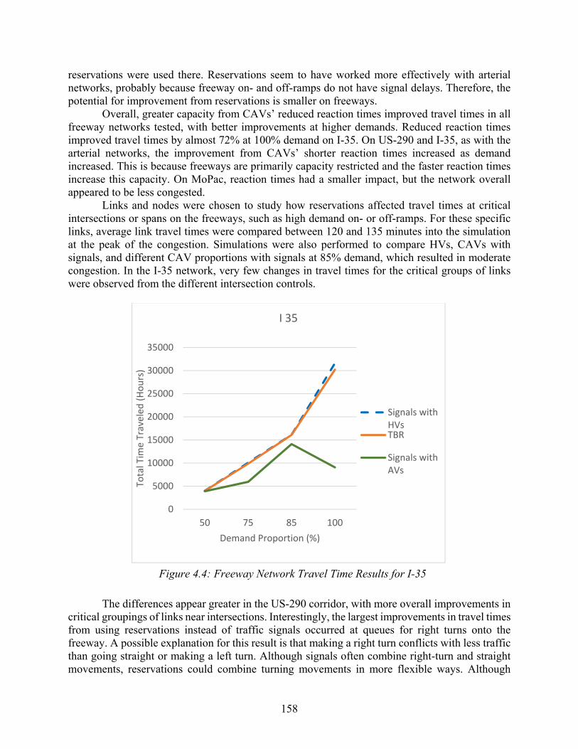
158

reservations were used there. Reservations seem to have worked more effectively with arterial networks, probably because freeway on- and off-ramps do not have signal delays. Therefore, the potential for improvement from reservations is smaller on freeways.

Overall, greater capacity from CAVs’ reduced reaction times improved travel times in all freeway networks tested, with better improvements at higher demands. Reduced reaction times improved travel times by almost 72% at 100% demand on I-35. On US-290 and I-35, as with the arterial networks, the improvement from CAVs’ shorter reaction times increased as demand increased. This is because freeways are primarily capacity restricted and the faster reaction times increase this capacity. On MoPac, reaction times had a smaller impact, but the network overall appeared to be less congested.

Links and nodes were chosen to study how reservations affected travel times at critical intersections or spans on the freeways, such as high demand on- or off-ramps. For these specific links, average link travel times were compared between 120 and 135 minutes into the simulation at the peak of the congestion. Simulations were also performed to compare HVs, CAVs with signals, and different CAV proportions with signals at 85% demand, which resulted in moderate congestion. In the I-35 network, very few changes in travel times for the critical groups of links were observed from the different intersection controls.

Figure 4.4: Freeway Network Travel Time Results for I-35

The differences appear greater in the US-290 corridor, with more overall improvements in critical groupings of links near intersections. Interestingly, the largest improvements in travel times from using reservations instead of traffic signals occurred at queues for right turns onto the freeway. A possible explanation for this result is that making a right turn conflicts with less traffic than going straight or making a left turn. Although signals often combine right-turn and straight movements, reservations could combine turning movements in more flexible ways. Although

0

5000

10000

15000

20000

25000

30000

35000

50 75 85 100

Tota

l Tim

e Tr

avel

ed (H

ours

)

Demand Proportion (%)

I 35

Signals withHVsTBR

Signals withAVs

159

larger improvements in travel times occurred at the observed right turns, improvements at left turns were also observed. Because US-290 has signals intermittently spaced throughout the model’s span, vehicles are frequently stopping at lights, causing signal delays, which can increase as the demand increases. Using the reservation system, the flow of traffic is stopped less frequently, if at all, reducing congestion along the freeway. Also, in the 290 network, analyzing the effects of reduced reaction times showed that improvements to travel times were made due to the reaction times and their respective capacity increases, but these improvements were less than those experienced due to reservations. It is also important to note that the use of 1s and 2s reaction times rather than 0.5s and 1s reaction times for the CAVs and HVs respectively did not affect travel times or any trends seen in the original reaction time simulations for any networks. In most cases, using reservations instead of signals doubled the improvements resulting from using CAVs. On US-290, reservations appear to have a positive effect on traffic flow and congestion in networks (freeway and arterial) that use signals to control intersections. Figure 4.5 depicts the results for MoPac and 290.

160

Figure 4.5: Freeway Network Travel Time Results for MoPac and US 290

4.3.3 Effects of Autonomous Vehicles on City Networks

For the downtown network of Austin (Figure 4.6), simulations were run at 100% demand for different proportions of CAVs in a traditional signal system. Additionally, the downtown Austin network was run with the TBR system at 100% CAVs, as shown in Table 4.1. Downtown Austin differs from the previous networks in that many route choices are available.

0

200

400

600

800

1000

1200

1400

1600

50 75 85 100

Tota

l Tim

e Tr

avel

ed (H

ours

)

Demand Proportion (%)

290

Signals withHVs

TBR

Signals withAvs

0

200

400

600

800

1000

1200

1400

50 75 85 100

Tota

l Tim

e Tr

avel

ed (H

ours

)

Demand Proportion (%)

Mopac

Signals withHVs

TBR

Signals withAVs

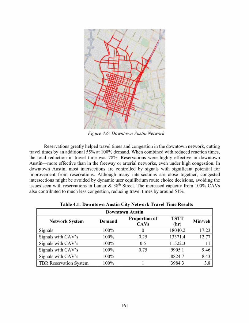
161

Figure 4.6: Downtown Austin Network

Reservations greatly helped travel times and congestion in the downtown network, cutting travel times by an additional 55% at 100% demand. When combined with reduced reaction times, the total reduction in travel time was 78%. Reservations were highly effective in downtown Austin—more effective than in the freeway or arterial networks, even under high congestion. In downtown Austin, most intersections are controlled by signals with significant potential for improvement from reservations. Although many intersections are close together, congested intersections might be avoided by dynamic user equilibrium route choice decisions, avoiding the issues seen with reservations in Lamar & 38th Street. The increased capacity from 100% CAVs also contributed to much less congestion, reducing travel times by around 51%.

Table 4.1: Downtown Austin City Network Travel Time Results

Downtown Austin

Network System Demand Proportion of

CAVs TSTT (hr)

Min/veh

Signals 100% 0 18040.2 17.23Signals with CAV’s 100% 0.25 13371.4 12.77Signals with CAV’s 100% 0.5 11522.3 11Signals with CAV’s 100% 0.75 9905.1 9.46Signals with CAV’s 100% 1 8824.7 8.43TBR Reservation System 100% 1 3984.3 3.8

162

4.4 Microsimulation using Autonomous Intersection Management (AIM)

Co-PI Peter Stone has developed two open-source traffic simulation software programs for CAVs: AIM, which provides highly detailed representations of small networks of intersections; and AORTA, which provides a more aggregate representation of a much larger (city-scale) network. Both accommodate mixed (traditional + CAV) traffic streams, traditional traffic control (signals), and reservation-based control for CAVs (who wish to reserve a safe path through the intersection without much delay).

The objective of the original AIM project was to create a scalable, safe, and efficient multi-agent framework for managing CAVs at intersections. AIM was designed for the time when all vehicles are fully autonomous. The AIM protocol exploits the fine control of CAVs to allow more vehicles simultaneously to cross an intersection, thus effectively reducing the delay of vehicles by orders of magnitude compared to traffic signals (Dresner and Stone 2005). In order to test the impact of the AIM protocol, the AIM simulator was developed. The AIM simulator validated the assumption that the AIM intersection control protocol is much more efficient compared to traditional traffic signals because it leverages the control and network capabilities of CAVs (Dresner and Stone 2008).

The project objectives of this newer microsimulation modeling sub-task were defined as follows:

1. Semi-CAVs – Inclusion of new, transitional vehicle types. The transition from current technologies to CAVs will occur gradually (along with retrofitting and addition of smart devices on board conventional vehicles), with vehicles gaining increasing autonomy and connectivity. For instance, a vehicle may have the ability to autonomously follow the car in front of it by staying in its lane and maintaining a constant following distance while traveling between intersections, but require a human driver to steer while turning through an intersection. We intend to adapt both AIM and AORTA to be able to model traffic that includes a mix of HVs, semi-CAVs, and full-CAVs.

2. Extending intersection control to handle mixed technology levels – In the case of vehicles that can follow autonomously, but not steer, such vehicles may be able to communicate with the intersection manager and obtain a reservation in more limited circumstances than could a vehicle with higher autonomy. For the case of HVs, we intend to add traffic light signaling that will coexist with AIM, this allows communication with both HVs as well as CAVs. These settings will be coded into the existing software, allowing for a wide range of scenario analyses under this sub-task.

As a first step in this research, one must evaluate the appropriateness of both AIM and AORTA as simulations of mixtures of HVs, semi-CAVs, and full-CAVs. Previous trials have found that the AIM simulator is well suited to such an adaptation due to its prior modeling of both full-CAVs and HVs. Thus, it was feasible to implement a variety of hybrid types of semi-CAVs and study a range of traffic mixtures as described below. On the other hand, the AORTA simulator does not meaningfully distinguish between HVs and CAVs, and there was not a straightforward path to implementing the sort of studies proposed in this task within AORTA. Therefore, focus was placed on subsequent research efforts associated with this task entirely on the AIM simulator.

163

4.5 Summary of Work

In order to achieve the above objectives with regards to AIM, the research focused on two main sub-objectives:

• SemiAIM protocol - SemiAIM is an enhanced version of the AIM protocol. As opposed to the AIM protocol, the SemiAIM protocol can correspond with semi-CAVs and HVs as well as full-CAVs. Figure 4.7 summarizes the interaction model of the SemiAIM protocol between human drivers, driver agents (with CAV or semi-CAV capabilities), and the Intersection Manager (IM). Inclusion that the vehicle has a single button to signal the driver agent to ask for a reservation is required. After the human driver presses the button, the driver agent will automatically send a request message to the IM on behalf of the human driver. It is also important that there is a clear Okay indicator (such as a green light) installed in the car that indicates when the request has been confirmed. After seeing the okay signal, the driver would have to actively pass control to the driver agent, again by pressing a single button. This way the driver will not be surprised by any sudden autonomous actions of the vehicle. The driver’s involvement in this procedure depends on the level of autonomous capabilities installed in the car. The different classifications of autonomous capabilities are described in Table 4.2. SemiAIM requires the human driver to perform only relatively simple driving maneuvers such as holding the steering wheel at a certain angle or driving as if under a traffic signal. These tasks are much simpler than other maneuvers such as lane changing and passing other vehicles, and thus should not be taxing to experienced human drivers.

• SemiAIM simulator - In order to experiment with the SemiAIM protocol, a SemiAIM simulator was devised. Based on the AIM simulator, SemiAIM is able to simulate semi-CAVs and human drivers as well as full-CAVs. Some experiments to test the efficiency of the SemiAIM protocol have been run using the SemiAIM simulator. These showed that (as expected) as the percentage of cars with autonomous capabilities increases, then each vehicle suffers less delays. Figure 4.8 presents the average delay per car while crossing the intersection (y-axis) against the ratio of CAVs/HVs (x-axis) for different types of autonomous capabilities. Traffic level was fixed at 360 vehicles/lane/hour.

Table 4.2: Semi-CAV Technologies

Vehicle Type Communication

Device Cruise Control

Adaptive Cruise Control

SA-ACC X X X

SA-CC X X

SA-Com X

164

Figure 4.7: Interaction between Human Drivers, Driver Agents, and the Intersection Manager

Figure 4.8: Average Delay vs. Different Ratio of Autonomous/Human Drivers at Traffic Level

of 360 Vehicles/Lane/Hour

165

Chapter 5. Improvement and Implementation of Dynamic Microtolling

This chapter introduces a novel tolling scheme denoted -tolling. -tolling approximates the marginal cost of each link using only two variables (current travel time and free-flow travel time) and one parameter. Due to its simplicity, -tolling is fast to compute, adaptive to current traffic, and accurate. We prove that, under some assumptions, -tolling results in tolls that are equivalent to the marginal cost and demonstrate that it can lead to near-optimal performance in practice.

5.1 Motivation and Problem Definition

This section defines the notion of user equilibrium (UE) and system optimum (SO). Applying tolls is then introduced as a mechanism that allows UE and SO to coincide. The marginal cost toll (MCT) policy is then presented, followed by some mesoscopic traffic models that approximate it. Discussions on some of the drawbacks of such meso-models are presented, which provide the motivation for the current study.

5.1.1 Computing User Equilibrium

Consider a directed network = ( , ), where and are the set of nodes and links respectively. Suppose that the demand (flow rates) between every pair of nodes is known. In this chapter the travel time, te, on a link ∈ is a function of its flow ( ) and is represented using a non-decreasing function ( ) (also called volume delay or link-performance functions). In practice, the Bureau of Public Roads (BPR) function ( ) = (1 + ( ) ) is commonly used

as the delay function, where is the free-flow travel time and is the capacity of link . Finally, and are parameters whose default values are 0.15 and 4, respectively.

When agents choose routes selfishly, a state of equilibrium, called user equilibrium (UE) (Wardrop 1952), is reached in which all used routes between an origin-destination (OD) pair have equal and minimal travel time. The link flow rates corresponding to this state can be obtained by solving a non-linear convex program that minimizes the Beckmann potential function (∑ ∈ ( )  ) (Beckmann et al. 1956). This objective ensures that the KKT (Karush-Kuhn-Tucker) conditions (Kuhn and Tucker 1951; Karush 1939) of the convex program correspond to Wardrop’s UE principle (Wardrop 1952). The constraints of the optimization problem include non-negativity and flow conservation constraints. This model, also known as the traffic assignment problem (see Patriksson [1994] for a thorough overview), has been widely studied because of the mathematically appealing properties associated with convex programming.

5.1.2 Computing System Optimum

The SO problem can be formulated using a set of constraints similar to those used for computing UE but replacing the objective function with ∑ ∈ ( ). As mentioned before, all agents do not experience equal and minimal travel times at the SO state, which incentivizes agents to switch routes. Instead, if an optimal tolling policy is applied, the flows resulting from a UE assignment in which agents minimize the generalized cost (time + toll) coincides with the SO

166

solution. MCT (Pigou 1920; Beckmann et al. 1956; Braess 1968) is one such policy, where each agent is charged a toll that is equal to the increase in travel time he or she inflicts on all other agents. Unfortunately, knowing in advance the marginal impact of an agent on traffic is infeasible in practice.

5.1.3 Approximating Marginal Cost Tolls

The focus of this chapter is presenting methods that approximate marginal costs. Most of these methods assume that demand on each link is constant. In such cases MCT can be formally defined as follows: given a link ( ) and flow ( ), the toll applied to equals the change in travel

time caused by an infinitesimal flow (( )

) multiplied by the number of agents currently on this

link ( ). A number of researchers have attempted to develop macro-models that approximate MCT

for a given system (Yang et al. 2004; Han and Yang 2009). However, a major drawback of such macro-models is that they are static and do not capture the time-varying nature of traffic. They also assume that the delay on each link is a function of its flow and hence neglect effects of intersections and traffic shocks. Although there has been some research on congestion pricing using finer traffic flow models, most of the existing models either assume complete knowledge of demand distribution over time (Wie and Tobin 1998; Joksimovic et al. 2005) or are restricted to finding tolls on freeways in which travelers choose only between parallel tolled and free general-purpose lanes (Gardner et al. 2013, 2015; Yin and Lou 2009). This limitation motivates us to employ a simulation framework to simulate traffic in a more realistic manner, evaluate the performance of existing macro-models, and develop new methods to determine optimal tolls while adapting to unknown and changing demand.

5.2 Simulation

In order to evaluate the effectiveness of different tolling models on traffic flow optimization, we used a modified version of the AIM microsimulator (Dresner and Stone 2008).

5.2.1 Autonomous Intersection Manager Simulator

AIM provides a multi-agent framework for simulating CAVs on a road network grid; it presents a realistic traffic flow model that allows experimenting with adaptive tolling. The AIM simulator uses two types of agents: intersection managers (one per intersection) and driver agents (one per vehicle). Intersection managers are responsible for directing the vehicles through the intersections, while the driver agents are responsible for controlling the vehicles to which they are assigned. To improve the throughput and efficiency of the system, the driver agents “call ahead” to the intersection manager and request a path reservation (space-time sequence) within the intersection. The intersection manager then determines whether or not this request can be met. If the intersection manager approves a driver agent’s request, the driver agent must follow the assigned path through the intersection. On the other hand, if the intersection manager rejects a driver agent’s request, the driver agent may not pass through the intersection but may attempt to request a new reservation.

At every intersection, the driver agent navigator runs an ∗ search (Hart et al. 1968) to determine the shortest path leading to the destination of the vehicle associated with it. The

167

navigator then directs the driver agent to drive via the shortest route. This behavior ensures that each vehicle acts greedily with respect to minimizing travel time. Next, the required enhancements to the standard AIM simulator (Dresner and Stone 2008) necessary to simulate realistic tolling experiments are outlined.

5.3 Enhancements to the AIM Simulator

In order to evaluate adaptive tolling using AIM, the following modifications were required:

• Link toll: each link ( ) in the road network is associated with a toll, , which can adapt in real time according to traffic conditions.

• Link travel time: each link stores (1) an estimated travel time, , that is based on real-time observed flow speed, and (2) an estimated free-flow travel time, , that is based on the link’s length divided by its speed limit.

• Route selection: when a car has several routes leading to its destination, the driver agent chooses the route ( = , , . . . , ) that minimizes ∑ ∈ × + , where is the monetary value of time.

• Value of Time: each driver agent is associated with a randomly generated that is drawn from a normal distribution. Monetary units are chosen such that the mean value is 1 per second, and assume a standard deviation of 0.2. represents the value (in cents for instance) of one second for the driver. A driver with = is willing to pay up to

in order to reduce travel time by 1 second.

5.3.1 Macroscopic Model

As part of this research we use a macroscopic model to approximate MCT. This model is used to solve convex programs using Algorithm B (Dial 2006). Algorithm B is a bush-based/origin-based algorithm, which exploits the fact that, at equilibrium, all used routes carrying demand from a particular origin must belong to an acyclic subgraph in which each destination can be reached from the origin (such a subgraph is also called a bush). At each iteration, the algorithm maintains a collection of bushes (one for each origin), shifts agents within a bush to minimize their generalized costs, and adds or removes links in a bush until equilibrium is reached. Closeness to equilibrium is measured using average excess cost, which represents the average of the difference between each agent’s generalized cost and the least cost path at the current flow solution. In the experiments presented in this chapter, the algorithm was terminated when the average excess cost of the flow solution dropped below a tolerance level of 10-13.

5.3.2 Example Road-Network

Figure 5.1 illustrates an exemplar road network demonstrating the impact of tolls that adapt to traffic demand. The speed limit across all roads is 25 meters per second. Each horizontal road is 142 meters long, and each vertical road is 192 meters long. A scenario was examined in which agents enter the network from a single source, the top road (incoming arrow), and leave the network from one of two destinations (outgoing arrows): D1 or D2. All roads are composed of two

168

lanes per direction and assumed to have infinite capacity66 except the two vertical roads in the middle of the network (congestible links #1 and #2), which possess only one lane (capacity = 1,908 agents per hour). An agent entering the system and heading towards D1 (or symmetrically D2) has two possible routes to choose from: a short route (668 m) or a long route (964 m). Each agent chooses one of the two routes according to the distance, traffic conditions, and tolls associated with it. This road network represents a special case where if most agents are heading to D1 (or symmetrically D2) then link #1 (#2) should be tolled, while link #2 (#1) should not. Define (or symmetrically 1 − ) to be the proportion of agents heading to 1 ( 2). The incoming traffic rate was set to 2160 agents per lane per hour.

Figure 5.1: Example Road Network within the AIM Simulator

5.3.3 Empirical Evaluation: Macroscopic Model

One of the main contributions of this report is an empirical demonstration that setting tolls based on macro-models MCT approximations can lead to suboptimal results when evaluated in a more realistic microsimulator. This section presents these empirical results, which motivate our new tolling scheme as presented in the next section. We report experimental results obtained from the adapted AIM simulator, using the road network described in the previous section (depicted in

66The capacity on roads with two lanes is higher than the rate in which agents are spawned. Hence, we consider such roads as having infinite capacity.

169

Figure 5.1). We define z (1-z) to be the percentage of cars going to D1 (D2). The incoming traffic rate was set to 2160 cars per lane per hour.

Table 5.1 presents these results. The left side of the table shows the empirical optimal and macro-model predicted toll values (imposed on link #2) for different z values. The right side shows average travel times when no tolls, static tolls, optimal tolls, macro-model tolls, and ∆-tolls are applied as calculated by the AIM simulator. The asterisk (*) indicates statistical significance over no tolls (using unpaired t-test with pvalue = 0.05).

Table 5.1: Toll Values and Travel Times

z Toll Values Average Travel Time (seconds)

Optimal Macro Model

No Tolls Static Tolls

Optimal Tolls

Macro Tolls

Δ-Tolls

0.0 15 14.8 46.0 47.6 40.9* 40.3* 40.5*

0.1 10 14.8 43.2 45.1 39.1* 39.3* 39.0*

0.2 10 14.8 38.4 40.8 35.8* 38.4 36.9*

0.3 10 14.8 34.3 35.1 33.8 37.7 33.1*

0.4 0 14.8 31.7 32.4 31.7 36.8 31.4

0.5 5 -5.3 30.8 31.2 30.8 30.9 30.9

0.6 5 -14.8 31.1 31.5 31.1 34.7 31.6

0.7 -5 -14.8 32.2 32.2 32.2 35.2 32.8

0.8 -10 -14.8 37.0 34.1* 34.1* 36.2 35.8*

0.9 -10 -14.8 40.7 36.2* 36.2* 36.8* 36.5*

1.0 -15 -14.8 43.1 39.0* 38.5* 38.1* 38.7*

5.3.4 Computing the Optimal Tolls

We start by computing the toll values that optimize average travel time for each ∈{0.0,0.1,0.2, . . . ,1} were computed by brute force. Consider tolling only congestible link #2. Tolling links that are not susceptible to congestion is unnecessary, as there is no congestion externality associated with travel on these links. Moreover, there is no reason to toll both congestible links simultaneously (#1 and #2) since any of the two possible routes (leading from source to ) includes exactly one of these links. A negative toll value for link #2 is symmetrical to a positive toll on link #1. There is a distinction between the optimal adaptive toll and the optimal static toll. The optimal adaptive toll is the toll value that minimizes travel time for a given value. The optimal static toll is the toll value that minimizes travel time over all values (assuming equal weighting of the values, i.e., all z values have the same probability), found to be −10 in this example. While it might seem like the optimal static toll should be zero, asymmetries in the model arising from differences between left and right turns affect junction delays and skew the optimal static toll to one side.

Optimal adaptive tolls for each value are presented in Table 5.1. Notice that as the value increases, the optimal toll steadily decreases. Intuitively, when all agents go to one destination ( = 0 or = 1), more of them choose the longer route to achieve the optimal system flow, thus requiring a more extreme toll. When ≈ 0.5, a zero toll is optimal since agents that choose their longer route will only make congestion worse for agents going to the other destination. As a result,

170

enforcing tolls for 0.2 < < 0.8 did not result in a significant improvement over enforcing no tolls.

5.3.5 Evaluating Optimal Tolls using a Macro-Model

Toll values calculated by the macro-model are also presented in Table 5.1, as well as average travel time under different tolling policies. Though the macro-model obtains near optimal results for the extreme values and = 0.5, it is sub-optimal for intermediate values. One explanation for this phenomenon is that the stylized congestion models assume that delays on a link are a function solely of flow on that link, ignoring interactions between links at intersections. For the extreme values this assumption is more reasonable because almost all agents on congestible links are heading in the same direction. However, for the intermediate values (excluding 0.5), the agents on the congestible links encounter traffic on the bottom horizontal link (by cars taking the longer route), causing changes in the capacity of the congestible links that cannot be captured by a stylized model. These results lead us to the following conclusions:

1. Tolls can reduce average travel time by up to 11% compared to applying no tolls (see = 0).

2. Static tolls might have a negative effect in some cases (see < 0.6).

3. The macro-model fails to achieve SO, in some cases reaching up to 10% suboptimality (see = 0.3).

Both static and adaptive macro-model based tolls (a) result in suboptimal performance and (b) require that the demand over all OD pairs is known and fixed. As a result, neither is applicable to real-world traffic. Thus, there is a need for a new tolling scheme that is dynamic, adaptive, and results in near-optimal traffic flow.

5.4 Delta-tolling Technique ( -tolling)

This section introduces the main technical contribution of this research, a new tolling scheme called “delta tolling” ( -tolling). Unlike macroscopic models, -tolling is adaptive to unknown and changing link capacities and demands. First, -tolling is defined and then proven, under mild assumptions, to be equivalent to MCT.

-tolling is defined over a directed network = ( , ) (a road network, for example) with a set of current flow values (traffic volume, for example). The output of -tolling is a set of toll values, one toll value per link. Let denote the current flow time on link ∈ . Recall that denotes the free-flow travel time and denotes the toll value assigned to link . For each link ( ), -tolling assigns a toll equivalent to the difference between the current flow time ( ) and the free-flow time ( ) multiplied by a parameter ( ). More formally: - = ( − ). As a rule of thumb, should be correlated to the mean VOT. High values result in high toll values, which are needed to influence agents with high VOT. Calculating - requires a constant amount of time. As a result, the complexity of computing tolls for an entire network is ( ).

In Box 1, proof is given that -tolling is equivalent to MCT under some conditions. This is a desirable property, since MCT results in SO (see Section 6.2). The assumptions under which the above statement holds are:

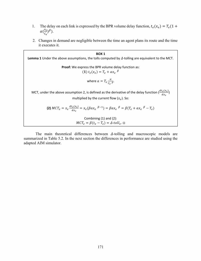
171

1. The delay on each link is expressed by the BPR volume delay function, ( ) = (1 +( ) ). 2. Changes in demand are negligible between the time an agent plans its route and the time

it executes it.

The main theoretical differences between -tolling and macroscopic models are

summarized in Table 5.2. In the next section the differences in performance are studied using the adapted AIM simulator.

BOX 1 Lemma 1 Under the above assumptions, the tolls computed by -tolling are equivalent to the MCT.

Proof: We express the BPR volume delay function as: ( ) ( ) = +  

where =   .

MCT, under the above assumption 2, is defined as the derivative of the delay function ( ( ))

multiplied by the current flow ( ). So:

(2) = ( ) = (   ) =   = ( +   − )

Combining (1) and (2): = ( − ) = - . □

172

Table 5.2: The Different Parameters, Variables, and Properties of ∆-tolling and Macro-Model Tolling

Macro-model Δ-tolling Parameters Required

α yes no β yes yes

Variables Required Demands yes no

Ce yes no Te yes yes te no yes

Properties Satisfied Adaptive no yes

MCT yes yes Note: MCT refers to approximating the marginal cost.

Although the assumptions made in this section might not hold in all possible traffic

networks, experimental results show that in realistic simulations, -tolling improves traffic flow and may achieve near optimal flow.

5.4.1 Empirical Evaluation of Delta-Tolling

This section analyzes the performance of -tolling on a representative road network. Findings are then generalized and shown to hold for randomly generated networks. Initially we examined the system performance when using -tolling on the example road network (presented in Figure 5.2). Table 5.1 also presents the average travel time for -tolling. Unlike the macro-model, -tolling achieves performance that is similar to the optimal. The toll values for -tolling are not reported as they are dynamically changing across the simulation.

Next, simulations were run to engender results for larger networks. In such networks finding the optimal tolls in a brute force manner is infeasible.67 For the following experiments, grid networks of size 3 × 3 are used. These grids include nine intersections (see Figure 5.2 for an example). Agents enter at the same rate of 300 agents per hour from any incoming lane (a road with three lanes, for example, spawns 900 agents per hour). Each agent entering the system is assigned one of two possible exit roads with equal probability (0.5). Each agent is also assigned two alternative exits. Exiting via an alternative exit imposes a predefined, randomly generated, delay.68 Alternative exits are justified because in many real-life scenarios several routes, usually of different length, may lead an agent to its destination. For example, while a driver exiting Manhattan and heading to Queens will prefer to use the Queens Midtown Tunnel, the driver can suffer some delay and instead exit from Ed Koch Queensboro Bridge or suffer a severe delay while exiting via Williamsburg Bridge. Following this logic, the simulated network is viewed as part of a larger road network in which agents may use paths outside of the network to reach their final destination.

67Examining different combinations of toll assignment to all links in the system leads to an exponential blowup. 68When each agent is assigned only one possible exit, distributing traffic becomes impossible in many cases. For such scenarios, imposing tolls did not have a positive effect in our experiments.

173

In the representative road network, each agent is assigned one of two destinations (D1, D2). A1 and A2 denote alternative destinations for D1 and D2 respectively. The time penalty associated with each alternative destination is given in parenthesis.

Figure 5.2: A Representative Road Network

Some roads in the simulated network are more congestible than others, i.e., the number of lanes varies. The number of lanes for each road was randomly selected as either 1, 2, 3, or 4. Simulations were run for 5000 seconds for each reported setting.69 In the following experiments, an upper bound on toll values was set equal to 25.70 The upper bound is set for two reasons: (1) avoiding overcharging in links with temporary heavy congestion; (2) avoiding oscillation in congestion caused by overpricing. Applying no cap on toll values resulted in up to 5% reduced utility. There are three different measurements to report:

• Time - the average travel time.

• Utility - the average utility (in cents). Where utility is defined for each agent as its travel time multiplied by its VOT plus the summation of tolls paid by it.

• Standardized Utility (SU) - toll revenue may be redistributed back to the drivers in the form of road improvements or tax reductions. Refund is the sum of collected tolls divided by the number of agents that exited the system. SU is defined as average utility minus refund.

5.4.2 Representative Road Network

The purpose of our first experiment is to determine how different values affect system performance. A single randomly generated instance of a 3 × 3 road network (depicted in Figure

69When running the simulator, in order to allow the system to balance, we excluded data from the first 500 seconds. 70The output from the macro-model contained no toll greater than 25. Hence, we deduced that greater tolls won’t have a positive affect and we set the cap accordingly.

174

5.2) was used for these simulations. Average travel time, utility, and SU for different values are presented in Figure 5.3. Notice that = 0 represent the case where no tolls are used.

Figure 5.3: Average Travel Time, Utility, and SU as a Function of β for the Representative

Road Network

Setting = 80 gives an improvement of 35.0% in average travel time over no tolls. Setting = 80 also gives an improvement of 35.0% for SU over no tolls. values greater than 80 result in average travel times that are not significantly worse or better. Increasing (up to 80) results in higher toll values that better distribute congestion. However, higher tolls also negatively impact utility as drivers are forced to pay more. Utility is maximized with = 8, which gives a 7.0% improvement over no tolls. Performance for setting tolls that are computed by the macro-model is shown as a dashed (red) line across the result graphs. -tolling outperforms macro-model tolling for ≥ 4 by up to 18% in both average travel time and SU. On the other hand, macro-model tolling exceeds by 6.3% when utility is considered. The main reason for the macro-model’s advantage with respect to utility is that -tolling imposes higher toll values. -tolling (with =8) collected a total of $1,921 while macro-model tolling collected only $825. Unfortunately, higher tolls are required to better distribute congestion and optimize system performance. On the other hand, SU is a more relevant measurement for performance comparison between the models. In real road networks, tolls are most often used to fund road maintenance, effectively redistributing the money collected back to the public. When SU is considered, delta tolling significantly outperforms the macro-model in all but very low . Moreover, macro-model tolling relies on static traffic conditions and so, unlike -tolling, it is not applicable to real-life, dynamic road networks.

5.4.3 Evaluating Optimal Tolls using a Macro-Model

In order to validate that the results obtained from a single randomized instance are representative, multiple simulations of the same experiment were run using 50 different randomized road networks. Each of these networks is a 3 × 3 grid, similar to the representative road network, but the exit roads, alternative exits, alternative exits’ delay, and number of lanes per road are randomized. Table 5.3 shows results for three representative values (8, 20, 80) compared to no tolling. = 8 and = 80 were chosen since they maximized performance with respect to utility and travel time/SU. = 20 represents a good balance between utility and travel time.

175

The advantage of -tolling is that it is responsive to changes in network topology. For the general case, -tolling achieves an improvement over no tolling of 29.2%, 9.3%, and 30.3% in Time, Utility, and SU respectively.

Table 5.3: Average Travel Time, Utility, and SU for β Values 8, 20, 80

β Time Utility SU

0.0 69.9 -70.0 -70.0

8.0 51.4* -63.5 -51.1*

20.0 50.3* -67.0 -49.8*

80.0 49.5* -76.6 -48.8* Note: These β values represent a trade-off between the three metrics. *Denotes a statistically significant improvement over no tolling (using a paired t-test with p_value=0.05).

5.5 Conclusions

This chapter considers applying tolls to road networks in order to direct the route choice of self-interested agents towards a system optimal. The notion of such a tolling scheme is becoming more practical as cars are becoming increasingly autonomous and the computational effort required to evaluate several alternative routes is becoming more feasible.

This chapter envelops two main contributions. First, using a traffic microsimulator (AIM), the empirical evidence suggests that stylized macroscopic traffic models are unable to approximate optimal tolls accurately. Given this finding and the fact that such models require full knowledge of demand and supply and assume that these remain fixed, the research team concluded that using such models to set tolls in real-life road networks is impractical. This conclusion leads to the second contribution, the presentation and evaluation of a new tolling scheme, denoted -tolling. Theoretical and empirical evidence shows that -tolling results in near-optimal system performance while being adaptive to traffic conditions and computationally feasible.

Ongoing research in Phase II of the project will include evaluating the performance of -tolling in dynamic environments, in which traffic demand and supply is time varying.

176

Chapter 6. Estimating the Safety Benefits of CAV Technologies

In this section, Najm’s (2007) latest pre-crash typology is presented first to help map the vehicle-to-vehicle (V2V), vehicle-to-infrastructure (V2I), and AV safety applications to specific crash types. In this way, safety benefits for each application can be estimated, using economic costs and functional-years lost per typical crash of each variety. The final part of this section introduces three technology-effectiveness scenarios to reflect uncertainty in how many crashes will benefit from such technologies and hopefully cover the range of the total economic benefits and quality-life-years to be saved by the various CV and AV applications.

6.1 Typology of Pre-Crash Situations

To appreciate the safety effects of having CAVs in the US, each crash’s pre-crash scenario typology was used here to estimate the economic cost savings and quality-life-years saved (Najm 2010 and Jermakian 2011). The pre-crash scenarios (or crash types, effectively) are based on the National Highway Traffic Safety Administration’s extensive General Estimates System (GES) year-2004 crash database (Najm 2010). Here, the same pre-crash typology is used, but results are based on the nation’s 2013 GES crash database. More details on the differences in these data sets can be found in Li and Kockelman (2016).

In this study, only light-duty vehicle crashes (i.e., those involving passenger cars, sports utility vehicles, vans, minivans, and pickup trucks) are investigated. The GES variables of Body Type and Special Use were queried to identify all light-duty vehicles. Body Type was set to include types 01–22, 28–41, and 45–49. Special Use was set equal to 0. Furthermore, in order to eliminate double counting of crashes in each scenario, pre-crash scenarios were updated by removing all scenarios in the number order via a process of elimination; in this way, the resulting frequency distribution sums to 100%. For example, one crash record can be assigned to pre-crash scenarios 1, 5, and 10, but this crash record will only belong to pre-crash scenario 1 because of its number order.

The 37 scenario identification codes can be used to select records from the GES database, and all pre-crash scenarios can be categorized into crash types, a more general term to segment or distinguish crashes. Table 6.1 illustrates each pre-crash scenario and the crash types to which they belong.

177

Table 6.1: Mapping of Crash Types to New Pre-Crash Scenario Typology No. Pre-Crash Scenario Crash Type 1 Vehicle failure

Run-off-road 2 Control loss with prior vehicle action 3 Control loss without prior vehicle action 4 Running red light

Crossing paths 5 Running stop sign 6 Road edge departure with prior vehicle maneuver

Run-off-road 7 Road edge departure without prior vehicle maneuver 8 Road edge departure while backing up 9 Animal crash with prior vehicle maneuver

Animal 10 Animal crash without prior vehicle maneuver 11 Pedestrian crash with prior vehicle maneuver

Pedestrian 12 Pedestrian crash without prior vehicle maneuver 13 Pedalcyclist crash with prior vehicle maneuver

Pedalcyclist 14 Pedalcyclist crash without prior vehicle maneuver 15 Backing up into another vehicle Backing 16 Vehicle(s) turning – same direction

Lane change 17 Vehicle(s) changing lanes – same direction 18 Vehicle(s) drifting – same direction 19 Vehicle(s) parking – same direction Parking 20 Vehicle(s) making a maneuver – opposite direction

Opposite direction 21 Vehicle(s) not making a maneuver – opposite direction 22 Following vehicle making a maneuver

Rear-end 23 Lead vehicle accelerating 24 Lead vehicle moving at lower constant speed 25 Lead vehicle decelerating 26 Lead vehicle stopped 27 LTAP/OD at signalized junctions

Crossing paths 28 Vehicle turning right at signalized junctions 29 LTAP/OD at non-signalized junctions 30 Straight crossing paths at non-signalized junctions 31 Vehicle(s) turning at non-signalized junctions 32 Evasive action with prior vehicle maneuver

Run-off-road 33 Evasive action without prior vehicle maneuver 34 Non-collision incident Non-collision 35 Object crash with prior vehicle maneuver

Object 36 Object crash without prior vehicle maneuver 37 Other Other

Source: Najm et al. 2007

6.2 Monetary and Non-Monetary Measure of the Pre-Crash Scenario Loss

Crashes incur both economic and non-economic costs. Economic costs reflect goods and services that must be purchased or lost productivity as a result of motor vehicle collisions (Blincoe 2015). This includes medical, legal and court, emergency service, insurance administration, travel delay, property damage and repairs, workplace losses, and lost productivity (at paid work and at home) costs. Comprehensive costs reflect additional social losses, including pain and suffering by

178

crash victims and their family members. In year 2010, quality-of-life losses from U.S. crashes were estimated to be 71% of all ($835 billion, comprehensive) U.S. crash costs (Blincoe 2015). Such non-economic losses are substantial and very important to appropriate evaluation of CAV technologies’ safety benefits and cost-effectiveness calculations.

With Najm’s (2007) identification codes of pre-crash scenarios used in the 2004 GES database, the frequency of each pre-crash scenario and the injury severity rating to a person is derived by using the National Safety Council’s KABCO scale in the 2013 GES crash records. The KABCO scale records injury severity as resulting in a death (K, for killed), an incapacitating injury (A), a non-incapacitating injury (B), a possible injury (C), or no apparent injury/property-damage only (O).

The KABCO ratings were translated into the Maximum Abbreviated Injury Scale (MAIS) to estimate economic costs and functional-years lost. MAIS levels of injury severity (for the crash victim who suffered the greatest injury) have seven categories, ranging from uninjured (MAIS0) to fatal (MAIS6), thus differing somewhat from the KABCO scale, which has six categories from fatal (K) to injury severity unknown (ISU). Here, Blincoe’s (2015) KABCO/MAIS translator, designed on data from the 2000-2008 NASS CDS, was employed, to convert all GES injury severities from KABCO to MAIS. Table 6.2 shows the KABCO/MAIS translator used in this paper.

Table 6.2: KABCO to MAIS Translator

MAIS0 MAIS1 MAIS2 MAIS3 MAIS4 MAIS5 MAIS6

K 0.0032 0.011 0.0019 0.0041 0.0027 0.0007 0.9765 1.00

A 0.0376 0.5782 0.1924 0.1259 0.0444 0.0171 0.0043 1.00

B 0.0906 0.1113 0.0348 0.0085 0.0014 0.0015 1.00

C 0.2188 0.7014 0.0674 0.0101 0.0021 0.0001 0.0001 1.00

O 0.8191 0.1759 0.0047 0.0002 0 0.0001 0 1.00

U 0.2429 0.5961 0.1039 0.0406 0.0047 0.0117 0 1.00

Source: NHTSA 2010

The economic and comprehensive unit costs of police-reported crashes were calculated in

U.S. Dollars for the year 2010 for each level of MAIS injury severity. Since this study’s estimates are based on the 2013 GES crash database, a cumulative rate of inflation between 2010 and 2013 was used (6.8% over 3 years). Table 6.3 shows the unit costs of economic and comprehensive costs of police-reported crashes in 2013, after adjusting for inflation.

179

Table 6.3: Unit Costs of Policed-Reported Crashes, 2013 Dollars

Crash Severity Economic costs: Cost per Crash

(2013$) Comprehensive Costs per Crash

(2013$)

MAIS0 $3,043 $3,043

MAIS1 $19,057 $43,925

MAIS2 $59,643 $424,376

MAIS3 $194,662 $1,056,758

MAIS4 $422,231 $2,602,338

MAIS5 $1,071,166 $5,970,187

MAIS6 $1,496,841 $9,786,218

Source: NHTSA 2015

6.3 Mapping the Advanced Safety Applications to the Specific Pre-Crash Scenarios

The first step of this estimation process involves mapping each advanced safety application to specific, applicable pre-crash scenarios. Najm et al. (2013) recently mapped many safety applications using V2V technology, including Forward Collision Warning (FCW), Intersection Movement Assist (IMA), Blind Spot Warning and Lane Changing Warning (BSW and LCW), Do Not Pass Warning (DNPW) and Control Loss Warning (CLW), to 17 pre-crash scenarios that can be addressed by V2V technology. For example, FCW can reduce the frequency of rear-end crash types, including the pre-crash scenarios of Following Vehicle Making a Maneuver, Lead Vehicle Moving at Lower Constant Speed, Lead Vehicle Decelerating and Lead Vehicle Stopped, but not Lead Vehicle Accelerating.

Intersection Movement Assist (IMA) can be mapped to certain crossing-paths crash types, including the pre-crash scenarios of Left Turn Across Path of Opposite Direction (LTAP/OD) at Non-Signalized Junctions, Straight Crossing Paths at Non-Signalized Junctions, and Vehicle(s) Turning at Non-Signalized Junctions. Cooperative Intersection Collision Avoidance Systems’ (CICAS’) objective is a cooperative intersection collision avoidance system to warn drivers of impending violations at traffic signals and stop signs (Maile and Delgrossi 2009). Compared with IMA, CICAS has a more powerful function, which warns drivers of running a red light or stop sign, or of other red-right or stop-sign runners; CICAS can also coordinate intersection movements, and thus take the place of the IMA, Red Light Violation Warning (RLVW), and Stop Sign Violation Warning (SSVW) systems. Therefore, CICAS addresses the following pre-crash scenarios: Running Red Light, Running Stop Sign, LTAP/OD at Signalized Junctions, Vehicle Turning Right at Signalized Junctions, LTAP/OD at Non-Signalized Junctions, Straight Crossing Paths at Non-Signalized Junctions, and Vehicle(s) Turning at Non-Signalized Junctions.

BSW and LCW technologies will benefit the Vehicle(s) Turning - Same Direction, Vehicle(s) Changing Lanes - Same Direction, and Vehicle(s) Drifting - Same Direction pre-crash scenarios. DNPW is expected to improve safety in Vehicle(s) Making a Maneuver - Opposite Direction and Vehicle(s) Not Making a Maneuver - Opposite Direction pre-crash situations. CLW can help avoid or mitigate the severity of Vehicle Failure, Control Loss with Prior Vehicle Action, and Control Loss Without Prior Vehicle Action pre-crash situations.

Road Departure Crash Warning (RDCW) is a combined application of Lateral Drift Warning (LDW) and Curve Speed Warning (CSW), which can warn drivers of impending road

180

departure (Wilson et al. 2007). The major function of the LDW is to monitor the vehicle’s lane position, lateral speed, and available maneuvering room by using a video camera to estimate the distances between the vehicle and the left and right lane boundaries, and is able to alert the driver when it appears the vehicle is likely to depart the lane of the road. The main contribution of CSW is to monitor vehicle speed and upcoming road curvature, and be able to alert the driver when the vehicle is approaching the upcoming curve at an unsafe speed. The RDCW application has the potential to improve the traffic safety of the pre-crash scenarios of Road Edge Departure With Prior Vehicle Maneuver, Road Edge Departure Without Prior Vehicle Maneuver, and Road Edge Departure While Backing Up, according to their definitions.

The Vehicle-to-Pedestrian (V2P) communication has the potential to detect pedestrians and pedalcyclists in a possible crash situation with a vehicle and warn the driver (Harding et al. 2014). To be more specific, the pedestrians can carry a device (such as a mobile phone) that can send out a safety signal using dedicated short-range communications (DSRC) and communicate with in-vehicle DSRC devices, so both the detected object (pedestrian or pedalcyclist) and the driver could be warned if a possible conflict arises. Four pre-crash scenarios, Pedestrian Crash with Prior Vehicle Maneuver, Pedestrian Crash Without Prior Vehicle Maneuver, Pedalcyclist Crash With Prior Vehicle Maneuver, and Pedalcyclist Crash Without Prior Vehicle Maneuver can be addressed by this safety application.

The safety applications described above emphasize CV technologies, such as V2V, V2I, and V2P. AV technology is rapidly advancing and will also play a key safety role by reducing or even eliminating many human-related factors leading to crashes, and greatly improve warning response times and decisions.

Lane-Keeping Assist (LKA) technology alerts the driver when lane deviations are detected in the vehicle. The system can also work in conjunction with the Radar Cruise Control system to help the driver steer and keep the vehicle on course (Bishop 2005). The LKA technology maps to pre-crash scenarios of Road Edge Departure With Prior Vehicle Maneuver, Road Edge Departure Without Prior Vehicle Maneuver, and Road Edge Departure While Backing Up, which are also addressed by the RDCW. Therefore, a combination of V2I and AV technologies (RDCW and LKA) has been mapped to these pre-crash scenarios.

Automatic Emergency Braking (AEB) can use radar, laser, or video to detect when obstructions or pedestrians are present and be automatically applied to avoid the collision or at least to mitigate the effects in the case that a collision is imminent. According to AEB’s function, almost all pre-crash scenarios can gain benefits from it, except the Non-Collision Incident.

Not all of Table 6.1’s pre-crash scenarios have been mapped to specific safety applications on the basis of CV and AV technologies. Due to the uncertain characteristics of the pre-crash scenarios of Non-Collision Incident and Other, there is no corresponding safety application to address. According to this situation, none of the safety applications mentioned above can avoid the accident or mitigate the accident severity. On the other hand, the Other pre-crash scenario may obtain benefit from those safety applications, so the combination impacts of CV and AV based safety applications will be exerted on this scenario.

Table 6.4 lists all the pre-crash scenarios and corresponding safety applications on the basis of CV and AV technologies, with the exception of Non-Collision Incident.

181

Table 6.4: Mapping Pre-crash Scenarios to CAV Technologies

No. Pre-Crash Scenario CV Safety Apps AV Safety Apps Fully Automated

Vehicle

1 Road Edge Departure With Prior Vehicle Maneuver Road Departure Warning

System

Automatic Emergency Braking +

Lane-Keeping Assist

Fully Automated Vehicle

2 Road Edge Departure Without Prior Vehicle Maneuver

3 Road Edge Departure While Backing Up

4 Control Loss With Prior Vehicle Action Control Loss Warning

Automatic Emergency Braking

Fully Automated Vehicle

5 Control Loss Without Prior Vehicle Action

6 Pedestrian Crash With Prior Vehicle Maneuver

Vehicle to Pedestrian 7 Pedestrian Crash Without Prior Vehicle Maneuver

8 Pedalcyclist Crash With Prior Vehicle Maneuver

9 Pedalcyclist Crash Without Prior Vehicle Maneuver

10 Vehicle(s) Turning - Same Direction Blind Spot/Lane Change

Warning Automatic Emergency

Braking Fully Automated

Vehicle 11 Vehicle(s) Changing Lanes - Same Direction

12 Vehicle(s) Drifting - Same Direction

13 Vehicle(s) Making a Maneuver - Opposite Direction Do Not Pass Warning

Automatic Emergency Braking

Fully Automated Vehicle

14 Vehicle(s) Not Making a Maneuver - Opposite Direction

15 Following Vehicle Making a Maneuver

Forward Collision Warning Automatic Emergency

Braking

16 Lead Vehicle Accelerating

17 Lead Vehicle Moving at Lower Constant Speed

18 Lead Vehicle Decelerating

19 Lead Vehicle Stopped

20 Running Red Light

Cooperative Intersection Collision Avoidance Systems

Automatic Emergency Braking

21 Running Stop Sign

22 LTAP/OD at Signalized Junctions

23 Vehicle Turning Right at Signalized Junctions

24 LTAP/OD at Non-Signalized Junctions

25 Straight Crossing Paths at Non-Signalized Junctions

26 Vehicle(s) Turning at Non-Signalized Junctions

182

No. Pre-Crash Scenario CV Safety Apps AV Safety Apps Fully Automated

Vehicle

27 Evasive Action With Prior Vehicle Maneuver

None

Automatic Emergency Braking

28 Evasive Action Without Prior Vehicle Maneuver

29 Animal Crash With Prior Vehicle Maneuver

30 Animal Crash Without Prior Vehicle Maneuver

31 Object Crash With Prior Vehicle Maneuver

32 Object Crash Without Prior Vehicle Maneuver

33 Vehicle Failure

34 Backing Up Into Another Vehicle

35 Vehicle(s) Parking - Same Direction Automatic Emergency Braking + Self Parking

System

36 Non-Collision Incident None

37 Other Combined Impacts of Safety

Applications Automatic Emergency

Braking

183

6.4 Effectiveness Assumptions of Safety Applications

Simply mapping the technology to the target pre-crash scenarios is not enough to estimate the safety benefits. A technology must successful correspond to pre-crash scenario(s) in order to complete the safety benefits analysis. The best way to understand the actual effectiveness of these technologies is to utilize field tests and collect data from real-life operation.

However, use of technologies mentioned above is still rare at present, and there is a lack of available field test data to conduct related research. Recent Insurance Institute for Highway Safety (IIHS) (2015) findings suggest a 23% crash reduction factor (CRF) for rear-end crashes in cars that have a FCW system enabled. When combined with active AEB, crash counts (of all types) appear to fall by 42% (IIHS 2015). However, few vehicles currently have AEB or FCW at all speed levels; for example, a Volvo S60 passenger car has this apply only at speeds less than 30 mi/hr. In fact, IIHS’ estimates are biased low, because they only apply at about half the speeds, so about half the crash benefits that true AEB (at all speeds) would yield. The CRF for rear-end crashes can be reduced by 84% with the combination of FCW and AEB in the moderate scenario.

The CRFs used in Table 6.6 reflect the Moderate-impact Scenario, assuming 100-percent market penetration of each CV and AV technology listed. CRFs for Conservative and Aggressive scenarios are set to be 75% and 125%, respectively, of the Moderate-impact scenario, but the CRF of every application would be maxed out 1.0. Tables 6.5 through 6.7 present the CRF assumptions across the nine settings (three scenarios and three application combinations). The CRFs of safety applications for other severity types are assumed to be 95%, 90%, 85%, and 80% of the reduction rate of fatal crashes, in the order of Incapacitating Injury (A) to Property Damage Only (O). Instead of assuming the same crash reduction rate for each safety application across all severity types, these assumed CRF values are expected to decrease as crash severity decreases, since some of the more severe crashes will be avoided, but not completely averted, and thus shift into the less severe categories. This means that the combined effect of all these safety technologies and applications is then applied to all “Other” crash types, with CRFs of 0.1, 0.2, and 0.3 for fatal crash reductions across the three impact scenarios.

184

Table 6.5: CRF (Cumulative) Assumptions of the Fatal Crashes in Conservative Scenario

No. Pre-Crash Scenario CV-Only Safety

Applications(CFR)

CV + AV Safety Applications Combined

(CFR)

CV + Full Automation Combined (CFR)

1 Road Edge Departure With Prior Vehicle Maneuver Road Departure Warning

System (0.18)

Automatic Emergency Braking +

Lane-Keeping Assist (0.36)

Fully Automated Vehicle (0.54)

2 Road Edge Departure Without Prior Vehicle Maneuver

3 Road Edge Departure While Backing Up

4 Control Loss With Prior Vehicle Action Control Loss Warning

(0.18)

Automatic Emergency Braking (0.27)

Fully Automated Vehicle (0.45) 5 Control Loss Without Prior Vehicle Action

6 Pedestrian Crash With Prior Vehicle Maneuver Vehicle to Pedestrian (Pedestrian)

(0.27)

Automatic Emergency Braking (0.45)

Fully Automated Vehicle (0.63) 7 Pedestrian Crash Without Prior Vehicle Maneuver

8 Pedalcyclist Crash With Prior Vehicle Maneuver Vehicle to Pedestrian (Pedalcyclist)

(0.18)

Automatic Emergency Braking (0.36)

Fully Automated Vehicle (0.54) 9 Pedalcyclist Crash Without Prior Vehicle Maneuver

10 Vehicle(s) Turning - Same Direction Blind Spot/Lane Change Warning

(0.27)

Automatic Emergency Braking (0.36)

Fully Automated Vehicle (0.63)

11 Vehicle(s) Changing Lanes - Same Direction 12 Vehicle(s) Drifting - Same Direction 13 Vehicle(s) Making a Maneuver - Opposite Direction

Do Not Pass Warning (0.18)

Automatic Emergency Braking (0.27)

Fully Automated Vehicle (0.45) 14

Vehicle(s) Not Making a Maneuver - Opposite Direction

15 Following Vehicle Making a Maneuver

Forward Collision Warning (0.21)

Automatic Emergency Braking (0.38)

Fully Automated Vehicle (0.54)

16 Lead Vehicle Accelerating 17 Lead Vehicle Moving at Lower Constant Speed 18 Lead Vehicle Decelerating 19 Lead Vehicle Stopped 20 Running Red Light

Cooperative Intersection Collision Avoidance

Systems (0.36)

Automatic Emergency Braking (0.54)

Fully Automated Vehicle (0.72)

21 Running Stop Sign 22 LTAP/OD at Signalized Junctions 23 Vehicle Turning Right at Signalized Junctions 24 LTAP/OD at Non-Signalized Junctions 25 Straight Crossing Paths at Non-Signalized Junctions 26 Vehicle(s) Turning at Non-Signalized Junctions

185

No. Pre-Crash Scenario CV-Only Safety

Applications(CFR)

CV + AV Safety Applications Combined

(CFR)

CV + Full Automation Combined (CFR)

27 Evasive Action With Prior Vehicle Maneuver

None (0)

Automatic Emergency Braking (0.18)

Fully Automated Vehicle (0.36)

28 Evasive Action Without Prior Vehicle Maneuver 29 Animal Crash With Prior Vehicle Maneuver 30 Animal Crash Without Prior Vehicle Maneuver 31 Object Crash With Prior Vehicle Maneuver 32 Object Crash Without Prior Vehicle Maneuver

33 Vehicle Failure Automatic Emergency

Braking (0.09)

Fully Automated Vehicle (0.18)

34 Backing Up Into Another Vehicle Automatic Emergency

Braking (0.54)

Fully Automated Vehicle (0.63)

35 Vehicle(s) Parking - Same Direction

Automatic Emergency Braking + Self-Parking

System (0.81)

Fully Automated Vehicle (0.81)

36 Non-Collision Incident None None

37 Other Combined Impacts of Safety Applications

(0.09)

Automatic Emergency Braking (0.18)

Fully Automated Vehicle (0.27)

186

Table 6.6: CRF (Cumulative) Assumptions of the Fatal Crashes in Moderate Scenario

No. Pre-Crash Scenario CV-Only Safety

Applications(CFR)

CV + AV Safety Applications Combined

(CFR)

CV + Full Automation Combined (CFR)

1 Road Edge Departure With Prior Vehicle Maneuver Road Departure Warning

System (0.20)

Automatic Emergency Braking +

Lane-Keeping Assist (0.40)

Fully Automated Vehicle (0.60)

2 Road Edge Departure Without Prior Vehicle Maneuver

3 Road Edge Departure While Backing Up

4 Control Loss With Prior Vehicle Action Control Loss Warning

(0.20)

Automatic Emergency Braking (0.30)

Fully Automated Vehicle (0.50) 5 Control Loss Without Prior Vehicle Action

6 Pedestrian Crash With Prior Vehicle Maneuver Vehicle to Pedestrian (Pedestrian)

(0.30)

Automatic Emergency Braking (0.50)

Fully Automated Vehicle (0.70) 7 Pedestrian Crash Without Prior Vehicle Maneuver

8 Pedalcyclist Crash With Prior Vehicle Maneuver Vehicle to Pedestrian (Pedalcyclist)

(0.20)

Automatic Emergency Braking (0.40)

Fully Automated Vehicle (0.60) 9 Pedalcyclist Crash Without Prior Vehicle Maneuver

10 Vehicle(s) Turning - Same Direction Blind Spot/Lane Change Warning

(0.30)

Automatic Emergency Braking (0.40)

Fully Automated Vehicle (0.70)

11 Vehicle(s) Changing Lanes - Same Direction 12 Vehicle(s) Drifting - Same Direction 13 Vehicle(s) Making a Maneuver - Opposite Direction

Do Not Pass Warning (0.20)

Automatic Emergency Braking (0.30)

Fully Automated Vehicle (0.50) 14 Vehicle(s) Not Making a Maneuver - Opposite Direction

15 Following Vehicle Making a Maneuver

Forward Collision Warning (0.23)

Automatic Emergency Braking (0.42)

Fully Automated Vehicle (0.60)

16 Lead Vehicle Accelerating 17 Lead Vehicle Moving at Lower Constant Speed 18 Lead Vehicle Decelerating 19 Lead Vehicle Stopped 20 Running Red Light

Cooperative Intersection Collision Avoidance

Systems (0.40)

Automatic Emergency Braking (0.60)

Fully Automated Vehicle (0.80)

21 Running Stop Sign 22 LTAP/OD at Signalized Junctions 23 Vehicle Turning Right at Signalized Junctions 24 LTAP/OD at Non-Signalized Junctions 25 Straight Crossing Paths at Non-Signalized Junctions 26 Vehicle(s) Turning at Non-Signalized Junctions

187

No. Pre-Crash Scenario CV-Only Safety

Applications(CFR)

CV + AV Safety Applications Combined

(CFR)

CV + Full Automation Combined (CFR)

27 Evasive Action With Prior Vehicle Maneuver

None

Automatic Emergency Braking (0.20)

Fully Automated Vehicle (0.40)

28 Evasive Action Without Prior Vehicle Maneuver 29 Animal Crash With Prior Vehicle Maneuver 30 Animal Crash Without Prior Vehicle Maneuver 31 Object Crash With Prior Vehicle Maneuver 32 Object Crash Without Prior Vehicle Maneuver

33 Vehicle Failure Automatic Emergency

Braking (0.10)

Fully Automated Vehicle (0.20)

34 Backing Up Into Another Vehicle Automatic Emergency

Braking (0.60)

Fully Automated Vehicle (0.70)

35 Vehicle(s) Parking - Same Direction

Automatic Emergency Braking + Self-Parking

System (0.90)

Fully Automated Vehicle (0.90)

36 Non-Collision Incident None None

37 Other Combined Impacts of Safety Applications

(0.10)

Automatic Emergency Braking (0.20)

Fully Automated Vehicle (0.30)

188

Table 6.7: CRF (Cumulative) Assumptions of the Fatal Crashes in Aggressive Scenario

No. Pre-Crash Scenario CV-Only Safety

Applications(CFR)

CV + AV Safety Applications Combined

(CFR)

CV + Full Automation Combined (CFR)

1 Road Edge Departure With Prior Vehicle Maneuver Road Departure Warning

System (0.22)

Automatic Emergency Braking +

Lane-Keeping Assist (0.44)

Fully Automated Vehicle (0.66)

2 Road Edge Departure Without Prior Vehicle Maneuver

3 Road Edge Departure While Backing Up

4 Control Loss With Prior Vehicle Action Control Loss Warning

(0.22)

Automatic Emergency Braking (0.33)

Fully Automated Vehicle (0.55) 5 Control Loss Without Prior Vehicle Action

6 Pedestrian Crash With Prior Vehicle Maneuver Vehicle to Pedestrian (Pedestrian)

(0.33)

Automatic Emergency Braking (0.55)

Fully Automated Vehicle (0.77) 7 Pedestrian Crash Without Prior Vehicle Maneuver

8 Pedalcyclist Crash With Prior Vehicle Maneuver Vehicle to Pedestrian (Pedalcyclist)

(0.22)

Automatic Emergency Braking (0.44)

Fully Automated Vehicle (0.66) 9 Pedalcyclist Crash Without Prior Vehicle Maneuver

10 Vehicle(s) Turning - Same Direction Blind Spot/Lane Change Warning

(0.33)

Automatic Emergency Braking (0.44)

Fully Automated Vehicle (0.77)

11 Vehicle(s) Changing Lanes - Same Direction 12 Vehicle(s) Drifting - Same Direction 13 Vehicle(s) Making a Maneuver - Opposite Direction

Do Not Pass Warning (0.22)

Automatic Emergency Braking (0.33)

Fully Automated Vehicle (0.55) 14 Vehicle(s) Not Making a Maneuver - Opposite Direction

15 Following Vehicle Making a Maneuver

Forward Collision Warning (0.25)

Automatic Emergency Braking (0.46)

Fully Automated Vehicle (0.66)

16 Lead Vehicle Accelerating 17 Lead Vehicle Moving at Lower Constant Speed 18 Lead Vehicle Decelerating 19 Lead Vehicle Stopped 20 Running Red Light

Cooperative Intersection Collision Avoidance

Systems (0.44)

Automatic Emergency Braking (0.66)

Fully Automated Vehicle (0.88)

21 Running Stop Sign 22 LTAP/OD at Signalized Junctions 23 Vehicle Turning Right at Signalized Junctions 24 LTAP/OD at Non-Signalized Junctions 25 Straight Crossing Paths at Non-Signalized Junctions 26 Vehicle(s) Turning at Non-Signalized Junctions

189

No. Pre-Crash Scenario CV-Only Safety

Applications(CFR)

CV + AV Safety Applications Combined

(CFR)

CV + Full Automation Combined (CFR)

27 Evasive Action With Prior Vehicle Maneuver

None (0)

Automatic Emergency Braking (0.22)

Fully Automated Vehicle (0.44)

28 Evasive Action Without Prior Vehicle Maneuver 29 Animal Crash With Prior Vehicle Maneuver 30 Animal Crash Without Prior Vehicle Maneuver 31 Object Crash With Prior Vehicle Maneuver 32 Object Crash Without Prior Vehicle Maneuver

33 Vehicle Failure Automatic Emergency

Braking (0.09)

Fully Automated Vehicle (0.22)

34 Backing Up Into Another Vehicle Automatic Emergency

Braking (0.66)

Fully Automated Vehicle (0.77)

35 Vehicle(s) Parking - Same Direction

Automatic Emergency Braking + Self-Parking

System (0.99)

Fully Automated Vehicle (0.99)

36 Non-Collision Incident None None

37 Other Combined Impacts of Safety Applications

(0.11)

Automatic Emergency Braking (0.22)

Fully Automated Vehicle (0.33)

190

These CRFs are then applied to the original crash counts (by KABCO severity) and translated to the MAIS severity scale (using Table 6.2’s values).

6.5 Crash Savings Results

Based on the results of this study, CV technologies, including V2V, V2I, and V2P, are estimated to save between $23 billion to $28 billion in economic costs each year, and as much as $96 billion to $117 billion in comprehensive costs each year in the U.S. Among the CV safety applications, the CICAS, mapped to intersection and traffic signal related pre-crash scenarios, is estimated to have the greatest potential to reduce crash costs, by preventing or mitigating the severity of crossing-path crashes, resulting in conservative estimated annual economic savings of $9.1 billion, or $34.1 billion annually in comprehensive cost savings.

Compared to the CV-based safety applications, AV technologies play a more significant role in improving traffic safety. The results are reasonable because AV technologies, particularly fully automated vehicles can avoid a human driver’s incorrect response to warnings that non-automated CVs may provide (e.g., forward collision warnings rather than automatic emergency braking [IIHS 2016]). AEB is the most beneficial AV-based safety application, without being fully automated. AEB alone can save between $23.5 billion and $28.8 billion in economic costs and $90 billion to $110 billion in comprehensive costs annually.

The results also indicate a promising future of fully automated and connected vehicles in terms of safety benefits, which can save between $97 billion to $119 billion in economic costs and $391 billion to $477 billion in comprehensive costs. This suggests that about 75% of total (police-reported) collision costs could be saved if vehicles were made fully autonomous and connected.

191

Table 6.8: Annual Crash Counts of U.S. Light-Duty-Vehicle Pre-Crash Scenarios (using 2013 GES crash records)

No. Pre-Crash Scenario Crash Count

per Year Relative

Frequency 1 Vehicle failure 44K 0.80% 2 Control loss with prior vehicle action 65K 1.18% 3 Control loss without prior vehicle action 393K 7.14% 4 Running red light 192K 3.49% 5 Running stop sign 36K 0.65% 6 Road edge departure with prior vehicle maneuver 85K 1.54% 7 Road edge departure without prior vehicle maneuver 441K 8.01% 8 Road edge departure while backing up 77K 1.40% 9 Animal crash with prior vehicle maneuver 3K 0.05%

10 Animal crash without prior vehicle maneuver 297K 5.39% 11 Pedestrian crash with prior vehicle maneuver 27K 0.49% 12 Pedestrian crash without prior vehicle maneuver 42K 0.76% 13 Pedalcyclist crash with prior vehicle maneuver 127K 2.31% 14 Pedalcyclist crash without prior vehicle maneuver 120K 2.18% 15 Backing up into another vehicle 22K 0.40% 16 Vehicle(s) turning – same direction 279K 5.07% 17 Vehicle(s) changing lanes – same direction 247K 4.48% 18 Vehicle(s) drifting – same direction 4K 0.07% 19 Vehicle(s) parking – same direction 95K 1.72% 20 Vehicle(s) making a maneuver – opposite direction 91K 1.65% 21 Vehicle(s) not making a maneuver – opposite direction 1.1M 20.21% 22 Following vehicle making a maneuver 202K 3.67% 23 Lead vehicle accelerating 268K 4.87% 24 Lead vehicle moving at lower constant speed 202K 3.67% 25 Lead vehicle decelerating 47K 0.85% 26 Lead vehicle stopped 136K 2.47% 27 LTAP/OD at signalized junctions 321K 5.83% 28 Vehicle turning right at signalized junctions 320K 5.81% 29 LTAP/OD at non-signalized junctions 125K 2.27% 30 Straight crossing paths at non-signalized junctions 78K 1.42% 31 Vehicle(s) turning at non-signalized junctions 9K 0.16% 32 Evasive action with prior vehicle maneuver 44K 0.80% 33 Evasive action without prior vehicle maneuver 65K 1.18% 34 Non-collision incident 393K 7.14% 35 Object crash with prior vehicle maneuver 192K 3.49% 36 Object crash without prior vehicle maneuver 36K 0.65% 37 Other 85K 1.54% Totals 5.5 Million/yr 100%

192

Table 6.9: Economic Costs and Comprehensive Costs of All U.S. Light-Duty-Vehicle Pre-Crash Scenarios (using 2013 GES crash records)

No. Pre-Crash Scenario Economic Costs

($M, 2013 Dollars)

Comprehensive Costs ($M, 2013

Dollars)

1 Vehicle failure $1,585 $6,567

2 Control loss with prior vehicle action $14,425 $70,886

3 Control loss without prior vehicle action $7,570 $28,833

4 Running red light $1,193 $4,070

5 Running stop sign $1,957 $8,564

6 Road edge departure with prior vehicle maneuver $13,419 $64,545

7 Road edge departure without prior vehicle maneuver $667 $1,693

8 Road edge departure while backing up $27 $91

9 Animal crash with prior vehicle maneuver $3,359 $9,651

10 Animal crash without prior vehicle maneuver $2,652 $14,567

11 Pedestrian crash with prior vehicle maneuver $5,086 $28,778

12 Pedestrian crash without prior vehicle maneuver $925 $3,857

13 Pedalcyclist crash with prior vehicle maneuver $1,221 $5,666

14 Pedalcyclist crash without prior vehicle maneuver $2,094 $5,502

15 Backing up into another vehicle $2,982 $10,873

16 Vehicle(s) turning – same direction $550 $1,795

17 Vehicle(s) changing lanes – same direction $6,948 $20,366

18 Vehicle(s) drifting – same direction $5,222 $14,640

19 Vehicle(s) parking – same direction $951 $5,926

20 Vehicle(s) making a maneuver – opposite direction $6,086 $30,212

21 Vehicle(s) not making a maneuver – opposite direction $121 $529

22 Following vehicle making a maneuver $2,495 $8,702

23 Lead vehicle accelerating $32,401 $100,159

24 Lead vehicle moving at lower constant speed $6,319 $21,815

25 Lead vehicle decelerating $7,167 $21,337

26 Lead vehicle stopped $8,172 $31,864

27 LTAP/OD at signalized junctions $883 $2,296

28 Vehicle turning right at signalized junctions $5,102 $19,310

29 LTAP/OD at non-signalized junctions $11,065 $41,088

30 Straight crossing paths at non-signalized junctions $9,151 $31,012

31 Vehicle(s) turning at non-signalized junctions $8 $24

32 Evasive action with prior vehicle maneuver $177 $666

33 Evasive action without prior vehicle maneuver $106 $556

34 Non-collision incident $173 $500

35 Object crash with prior vehicle maneuver $1,413 $6,026

36 Object crash without prior vehicle maneuver $4 $9

37 Other $5,423 $21,879

Annual Totals $169 billion $645 billion

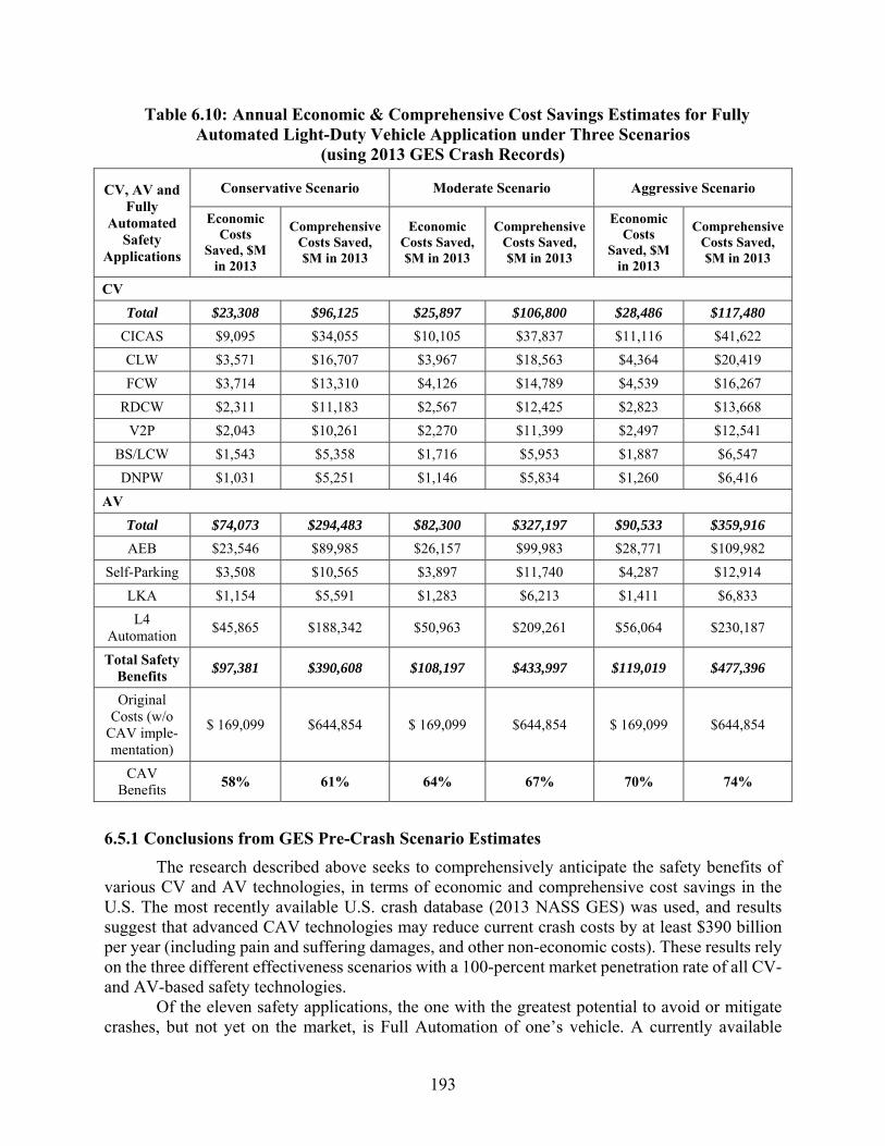
193

Table 6.10: Annual Economic & Comprehensive Cost Savings Estimates for Fully Automated Light-Duty Vehicle Application under Three Scenarios

(using 2013 GES Crash Records)

CV, AV and Fully

Automated Safety

Applications

Conservative Scenario Moderate Scenario Aggressive Scenario

Economic Costs

Saved, $M in 2013

Comprehensive Costs Saved, $M in 2013

Economic Costs Saved, $M in 2013

Comprehensive Costs Saved, $M in 2013

Economic Costs

Saved, $M in 2013

Comprehensive Costs Saved, $M in 2013

CV

Total $23,308 $96,125 $25,897 $106,800 $28,486 $117,480

CICAS $9,095 $34,055 $10,105 $37,837 $11,116 $41,622

CLW $3,571 $16,707 $3,967 $18,563 $4,364 $20,419

FCW $3,714 $13,310 $4,126 $14,789 $4,539 $16,267

RDCW $2,311 $11,183 $2,567 $12,425 $2,823 $13,668

V2P $2,043 $10,261 $2,270 $11,399 $2,497 $12,541

BS/LCW $1,543 $5,358 $1,716 $5,953 $1,887 $6,547

DNPW $1,031 $5,251 $1,146 $5,834 $1,260 $6,416

AV

Total $74,073 $294,483 $82,300 $327,197 $90,533 $359,916

AEB $23,546 $89,985 $26,157 $99,983 $28,771 $109,982

Self-Parking $3,508 $10,565 $3,897 $11,740 $4,287 $12,914

LKA $1,154 $5,591 $1,283 $6,213 $1,411 $6,833

L4 Automation

$45,865 $188,342 $50,963 $209,261 $56,064 $230,187

Total Safety Benefits

$97,381 $390,608 $108,197 $433,997 $119,019 $477,396

Original Costs (w/o

CAV imple-mentation)

$ 169,099 $644,854 $ 169,099 $644,854 $ 169,099 $644,854

CAV Benefits

58% 61% 64% 67% 70% 74%

6.5.1 Conclusions from GES Pre-Crash Scenario Estimates

The research described above seeks to comprehensively anticipate the safety benefits of various CV and AV technologies, in terms of economic and comprehensive cost savings in the U.S. The most recently available U.S. crash database (2013 NASS GES) was used, and results suggest that advanced CAV technologies may reduce current crash costs by at least $390 billion per year (including pain and suffering damages, and other non-economic costs). These results rely on the three different effectiveness scenarios with a 100-percent market penetration rate of all CV- and AV-based safety technologies.

Of the eleven safety applications, the one with the greatest potential to avoid or mitigate crashes, but not yet on the market, is Full Automation of one’s vehicle. A currently available

194

technology, AEB, also offers substantial safety rewards, with an estimated economic savings of $23.5 to $28.8 billion each year, assuming full adoption across the U.S., along with current crash counts. Among the CV-based safety applications, CICAS is estimated to offer the greatest economic and comprehensive cost savings. Overall, AV-based technologies are expected to offer far more safety benefits than CV-based technologies, as expected, since automation proactively avoids human errors during travel, rather than simply warning human drivers about possible conflicts.

There is little doubt that various CAV technologies will offer significant safety benefits to transportation system users. However, the actual effectiveness of these technologies will not be known until sufficient real-world data have been collected and analyzed. Here, their effectiveness assumes 100-percent market access and use (thus technologies are available to all motorized vehicle occupants and are not disabled by those occupants), as well as different success rates under several assumption scenarios. Such assumptions come with great uncertainty surrounding the interaction between CAV systems and drivers/travelers. More on-road deployment and testing will be helpful to decrease the uncertainty of benefit analysis of CAV systems in terms of traffic safety improvement, alongside simulated driving situations. It is also important to note that connectivity is not needed in many cases, when AV cameras will suffice. However, CICAS does require a roadside device that is able to communicate quickly with all vehicles. NHTSA is likely to require DSRC on all new vehicles beginning in model year 2020 (Harding et al. 2014). Therefore, connectivity may become widely available much more quickly than high levels of automation, in terms of fleet mix over time. Older vehicles may be retrofitted with connectivity soon after, when costs are low (e.g., $100 for add-ons to existing vehicles (Bansal and Kockelman 2015) and the benefits of connectivity more evident nation-wide.

It is also noteworthy that GES crash records have even more attributes than those used here, including road types and weather conditions at time of crash. Future work may do well to focus on anticipating technology-specific safety benefits with more hierarchical pre-crash scenarios, combined with road types and weather conditions. Furthermore, the database used in this study only contains GES crash records, therefore representing only U.S. driving context. For more detailed results, local crash databases, and databases in other countries, can be queried, which may suggest different benefit rankings and magnitudes.

6.6 Crash Estimates using Safety Surrogate Assessment Model (SSAM)

It is difficult to anticipate the crash benefits C/AV technologies will provide, especially without certain details of each crash. Another method for inferring crash-related benefits, beyond the US crash counts and pre-crash scenario categorization used above, is to simulate traffic flows with and without C/AV technologies on board, and keep track of near-misses and other details that microsimulation models can detect. The FHWA’s Safety Surrogate Assessment Model (SSAM) is a tool for tracking such metrics.

6.6.1 Introduction and Definitions

SSAM analyzes trajectory data, in the form of a .trj file from traffic-microsimulation software, such as VisSim, and identifies conflicts. Conflicts are defined as situation in which two vehicles will collide unless action is taken, and are categorized into Unclassified, Crossing, Rear End, and Lane Change. For each conflict identified, there are several surrogate safety measures that include the following:

195

• Minimum time-to-collision (TTC)

• Minimum post-encroachment time (PET)

• Initial deceleration rate (DR)

• Maximum deceleration rate (MaxD)

• Maximum speed (MaxS)

• Maximum speed differential (DeltaS)

• Vehicle velocity change had the event proceeded to a crash (DeltaV)

Table 6.11: SSAM Measures and Definitions

SSAM Measure

Definitions

TTC The minimum time-to-collision value observed during the conflict. This estimate is based on the current location, speed, and trajectory of two vehicles at a given instant.

PET The minimum post encroachment time observed during the conflict. Post encroachment time is the time between when the first vehicle last occupied a position and the second vehicle subsequently arrived at the same position. A value of 0 indicates an actual collision.

MaxS The maximum speed of either vehicle throughout the conflict (i.e., while the TTC is less than the specified threshold). This value is expressed in feet per second or meters per second, depending on the units specified in the corresponding trajectory file.

DeltaS

The difference in vehicle speeds as observed at tMinTTC. More precisely, this value is mathematically defined as the magnitude of the difference in vehicle velocities (or trajectories), such that if v1 and v2 are the velocity vectors of the first and second vehicles respectively, then DeltaS = || v1 - v2 ||. Consider an example where both vehicles are traveling at the same speed, v. If they are traveling in the same direction, DeltaS = 0. If they have a perpendicular crossing.

DR

The initial deceleration rate of the second vehicle. Note that in actuality, this value is recorded as the instantaneous acceleration rate. If the vehicle brakes (i.e., reacts), this is the first negative acceleration value observed during the conflict. If the vehicle does not brake, this is the lowest acceleration value observed during the conflict. This value is expressed in feet per second or meters per second, depending on the units specified in the corresponding trajectory file.

MaxD

The maximum deceleration of the second vehicle. Note that in actuality, this value is recorded as the minimum instantaneous acceleration rate observed during the conflict. A negative value indicates deceleration (braking or release of gas pedal). A positive value indicates that the vehicle did not decelerate during the conflict. This value is expressed in feet per second or meters per second, depending on the units specified in the corresponding trajectory file.

MaxDeltaV The maximum DeltaV value of either vehicle in the conflict. This is a surrogate for the severity of the conflict, calculated assuming a hypothetical collision of the two vehicles in the conflict.

The surrogate measures focused on in this paper are Max S, MaxDelta V, and MaxD. Focus

is directed on Max S and MaxDeltaV because they are related to severity of a potential collision, and MaxD because it represents how well, on average, vehicles avoided collisions. From the SSAM Manual, TTC and PET are meant to indicate likelihood of a conflict, as PET = 0 indicates an actual collision, but they were not included in this analysis because of the nature of the EDMs.

196

The vehicles are already following quite close to each other, producing lower TTC and PET values, which inflate the number of conflicts recognized by SSAM. Therefore, for driver models used in VisSim, TTC and PET do not give a good indication of the likelihood of a collision.

6.6.2 Urban Roadway Bottlenecks

Table 6.12 provides bottleneck conflict results while Table 6.13 summarizes the percentage decrease in total number of conflicts between 100% human-driven vehicles (HVs) and 100% AVs, for low, medium, and high flows. See Figures 6.1–6.3 for a plot of every conflict type at their respective flows.

Table 6.12: Bottleneck Conflict Results Disaggregated by Type Percent Flow Total Unclassified Crossing Rear End Lane Change

Low

100% HV 5 0 0 5 0

25% AV 9 0 0 9 0

50% AV 7 0 0 7 0

75% AV 4 0 0 4 0

100% AV 3 0 0 3 0

Medium

100% HV 137 0 0 125 12

25% AV 115 0 0 106 9

50% AV 85 0 0 79 6

75% AV 50 0 0 42 8

100% AV 17 0 0 8 9

High

100% HV 1972 0 0 1547 425

25% AV 1741 0 1 1307 433

50% AV 1393 0 0 915 478

75% AV 1064 0 0 608 456

100% AV 684 0 0 256 428

Table 6.13: Percent Difference in Conflicts Between HVs and AVs

Percent Decrease between 100% HV and 100% AV Low 40% Medium 88% High 65%

197

Figure 6.1: Low-Flow Conflicts Disaggregated by Type

Figure 6.2: Medium-Flow Conflicts Disaggregated by Type

0

1

2

3

4

5

6

7

8

9

10

Total Unclassified Crossing Rear End Lane Change

Num

ber o

f Con

flict

s

Type of Conflict

All Human

25% AV

50% AV

75% AV

100% AV

0

20

40

60

80

100

120

140

160

Total Unclassified Crossing Rear End Lane Change

Num

ber o

f Con

flict

s

Type of Conflict

All Human

25% AV

50% AV

75% AV

100% AV

198

Figure 6.3: High-Flow Conflicts Disaggregated by Type

At low flow, the MaxDeltaV values are greater than only HVs with 25 and 50% AVs, but then decrease for the 75 and 100% AVs. At medium and high flow, the values are lower for all AV percentages, but only noticeably for 100% AVs. MaxS also decreases significantly between 100% HV and 75% AV/100% AV for all flow volumes. For example, at medium flow, the MaxS for all HVs is 29.09 m/s, while at 100% AVs it is 14.84 m/s, which is almost a 50% decrease. Table 6.14 displays the surrogate safety measures from the SSAM output, and Table 6.15 summarizes the percentage differences between the HV and AV EDMs.

Table 6.14: Bottleneck Surrogate Safety Measures (Number of Measures) Mean Value 100% HV 25% AV 50% AV 75% AV 100% AV

Low

MaxS 25.56 29.38 27.55 20.72 16.52

MaxDeltaV 3.96 5 4.71 3.62 2.53

MaxD -4.66 -5.49 -5.15 -1.76 -0.27

Medium

MaxS 29.09 29.18 27.61 25.51 14.84

MaxDeltaV 5.18 5.13 4.5 4.5 2.54

MaxD -6.3 -6.2 -5.94 -6.09 -3.52

High

MaxS 20.92 20.24 18.83 17.47 14.7

MaxDeltaV 4.71 4.69 4.14 3.83 2.98

MaxD -5.5 -5.56 -5.32 -4.96 -4.62

0

500

1000

1500

2000

2500

Total Unclassified Crossing Rear End Lane Change

Num

ber o

f Con

flict

s

Type of Conflict

All Human

25% AV

50% AV

75% AV

100% AV

199

Table 6.15: Percent Differences in Safety Measures between HVs and AVs (Bottleneck, Number of Measures)

Percent Difference 25% AV 50% AV 75% AV 100% AV

Low

MaxS 15 8 -19 -35

MaxDeltaV 26 19 -9 -36

MaxD 18 11 -62 -94

Medium

MaxS 0 -5 -12 -49

MaxDeltaV -1 -13 -13 -51

MaxD -2 -6 -3 -44

High

MaxS -3 -10 -16 -30

MaxDeltaV 0 -12 -19 -37

MaxD 1 -3 -10 -16

This data indicates that AVs are safer than HVs in a bottleneck situation, especially as the

percentage of AVs increases. At 50% AVs, the data only agrees at medium and high flows, and at only 25% AVs the data provides mixed results. More simulations on a variety of bottleneck networks will need to be run to draw concrete conclusions.

6.6.3 Four-way Intersections

Table 6.16 provides data on four-way intersection conflicts disaggregated by type while Table 6.17 provides data on four-way intersection surrogate safety measures.

Table 6.16: Four-way Intersection Conflicts Disaggregated by Type (Number of Conflicts)

Human External Driver Model and AV External Drive Model

Summary Total Unclassified Crossing Rear End Lane Change

100% HV 25 0 23 0 2

25% AV 25 0 23 0 2

50% AV 24 0 22 0 2

75% AV 24 0 22 0 2

100% AV 24 0 22 0 2

Figure 6.4 summarizes the total number of conflicts predicted by SSAM, for the four-way

intersection simulation. The data does not correspond to expected trends, based on the results seen from the other simulations. There is no variation in the number of conflicts between the different percentages of AV flow.

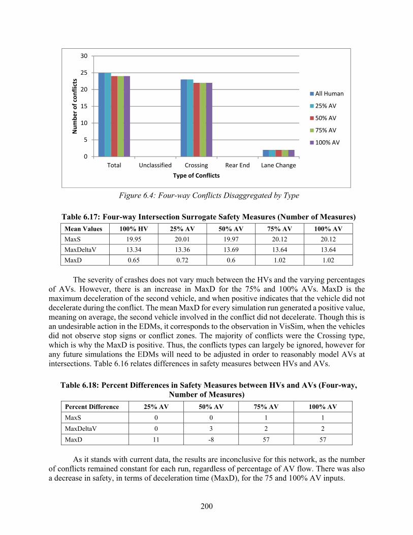
200

Figure 6.4: Four-way Conflicts Disaggregated by Type

Table 6.17: Four-way Intersection Surrogate Safety Measures (Number of Measures)

Mean Values 100% HV 25% AV 50% AV 75% AV 100% AV

MaxS 19.95 20.01 19.97 20.12 20.12

MaxDeltaV 13.34 13.36 13.69 13.64 13.64

MaxD 0.65 0.72 0.6 1.02 1.02

The severity of crashes does not vary much between the HVs and the varying percentages

of AVs. However, there is an increase in MaxD for the 75% and 100% AVs. MaxD is the maximum deceleration of the second vehicle, and when positive indicates that the vehicle did not decelerate during the conflict. The mean MaxD for every simulation run generated a positive value, meaning on average, the second vehicle involved in the conflict did not decelerate. Though this is an undesirable action in the EDMs, it corresponds to the observation in VisSim, when the vehicles did not observe stop signs or conflict zones. The majority of conflicts were the Crossing type, which is why the MaxD is positive. Thus, the conflicts types can largely be ignored, however for any future simulations the EDMs will need to be adjusted in order to reasonably model AVs at intersections. Table 6.16 relates differences in safety measures between HVs and AVs.

Table 6.18: Percent Differences in Safety Measures between HVs and AVs (Four-way, Number of Measures)

Percent Difference 25% AV 50% AV 75% AV 100% AV

MaxS 0 0 1 1

MaxDeltaV 0 3 2 2

MaxD 11 -8 57 57

As it stands with current data, the results are inconclusive for this network, as the number

of conflicts remained constant for each run, regardless of percentage of AV flow. There was also a decrease in safety, in terms of deceleration time (MaxD), for the 75 and 100% AV inputs.

0

5

10

15

20

25

30

Total Unclassified Crossing Rear End Lane Change

Num

ber o

f con

flict

s

Type of Conflicts

All Human

25% AV

50% AV

75% AV

100% AV

201

6.6.4 On Freeway On-Ramps and Off-Ramps

Table 6.19 and Figure 6.5 provide on-ramp/off-ramp conflicts disaggregated by type.

Table 6.19: On-Ramp/Off-Ramp Conflicts Disaggregated by Type (Number of Conflicts)

Human External Driver Model and AV External Drive Model

Summary Total Unclassified Crossing Rear End Lane Change

100% HV 117 0 0 96 21

25% AV 119 0 0 97 22

50% AV 85 0 0 70 15

75% AV 81 0 0 65 16

100% AV 60 0 0 46 14

Figure 6.5: On-Off Ramp Conflicts Disaggregated by Type

For this network there was a slight increase of two conflicts during the 25% AV flow; however, this is an anomaly among the other data sets. In general, Table 6.20 shows that as the percentage of AV’s increases, the number of conflicts decreases, with the least number of conflicts occurring at 100% AVs. The most drastic decreases in conflicts occur with Rear End types. There was a slight decrease in the severity of crashes as the percentages of AVs increased, as well as a better deceleration response. The results indicate that AVs decrease the number of conflicts for networks involving entrance and exit ramps onto or off of a freeway.

0

20

40

60

80

100

120

140

Total Unclassified Crossing Rear End Lane Change

Num

ber o

f Con

flict

s

Conflict Types

All Human

25% AV

50% AV

75% AV

100% AV

202

Table 6.20: On-Off Ramp Surrogate Safety Measures (Number of Measures)

Mean Values 100% HV 25% AV 50% AV 75% AV 100% AV

MaxS 30.28 30.18 30.64 29.22 28.45

MaxDeltaV 4.07 4.32 4.41 3.71 3.23

MaxD -3.72 -3.52 -3.51 -3.27 -2.66

Intersection of I-35 and Wells Branch Parkway

It was found through the simulations for the network intersection of I-35 and Wells Branch Parkway that the number of conflicts comprehensively decreased with the addition of AVs in the traffic. Figure 6.6 summarizes the conflicts across various concentrations of AVs.

Figure 6.6: Intersection of I-35 and Wells Branch Parkway Conflicts Disaggregated by Type

At the specified flow, the MaxDeltaV and DeltaS values were found to decrease consistently with the increase in the concentration of AVs at this intersection. MaxS, also decreases significantly between 100% HV and 50% AV/100% AV. For example, the MaxS for all HVs is 19.28 m/s, while at 100% AVs it is 17.87 m/s, which is almost an 8% decrease. Similarly, the DeltaS for all HVs is 17.21 m/s, while at 100% AVs it is 9.36 m/s, which is almost a 45% decrease. Finally, the MaXDeltaV for all HVs is 9.07 m/s, while at 100% AVs it is 4.94 m/s, which is almost a 45% decrease. Tables 6.21 and 6.22 summarize the total number of conflicts and other measures for the various scenarios predicted by SSAM.

The following results were observed for 100% HVs at the intersection of I-35 and Wells Branch Parkway.

0

10000

20000

30000

40000

50000

60000

Total Crossing Rear End Lane Change

Num

ber o

f con

flict

s

Type of conflicts

100% Human vehicles

100% Avs

%0% Human and 50% Avs

203

Table 6.21: Intersection of I-35 and Wells Branch Parkway Conflict Summary (Number of Conflicts)

Summary Total Unclassified Crossing Rear End Lane Change

Total 53605 0 0 50176 3429

Run 1 11440 0 0 11106 334

Run 2 2632 0 0 2262 370

Run 3 1617 0 0 1284 333

Run 4 1697 0 0 1292 405

Run 5 3350 0 0 2995 355

Run 6 1176 0 0 921 255

Run 7 1143 0 0 898 245

Run 8 27168 0 0 26719 449

Run 9 1576 0 0 1230 346

Run 10 1806 0 0 1469 337

Table 6.22: Intersection of I-35 and Wells Branch Parkway Surrogate Safety Measures (Number of Measures)

SSAM Measure Min Max Mean Variance

TTC 0 1.5 0.07 0.07

PET 0 3.8 0.04 0.04

MaxS 0 34.5 19.28 6.01

DeltaS 0 24.07 17.21 23.02

DR -8.39 3 -3.92 7.05

MaxD -8.44 3 -6.45 3.79

MaxDeltaV 0 13.71 9.07 6.51

Tables 6.23 and 6.24 provide the results for 100% AVs for the intersection of I-35 and

Wells Branch Parkway, while Tables 6.25 and 6.26 provide the results for 50% AV and 50% HVs at that intersection.

204

Table 6.23: Intersection of I-35 and Wells Branch Parkway Conflict Summary (Number of Crashes)

Summary Total Unclassified Crossing Rear End Lane Change

Total 7035 0 3 3278 3754

Run 1 825 0 1 392 432

Run 2 787 0 0 356 431

Run 3 653 0 0 315 338

Run 4 749 0 0 365 384

Run 5 704 0 0 310 394

Run 6 783 0 1 376 406

Run 7 478 0 0 175 303

Run 8 563 0 0 251 312

Run 9 868 0 1 407 460

Run 10 625 0 0 331 294

Table 6.24: Intersection of I-35 and Wells Branch Parkway Surrogate Safety Measures (Number of Measures)

SSAM Measure Min Max Mean Variance

TTC 0 1.5 0.4 0.29

PET 0 4.8 0.28 0.27

MaxS 1.45 32.73 17.87 14.56

DeltaS 0 25.58 9.36 23.45

DR -8.19 3.37 -4.29 12.28

MaxD -8.33 3.37 -5.08 12.54

MaxDeltaV 0 13.99 4.94 6.6

Table 6.25: Intersection of I-35 and Wells Branch Parkway Conflicts Summary (Number of Conflicts)

Summary Total Unclassified Crossing Rear End Lane Change

Total 13350 0 2 9477 3871

Run 1 1325 0 0 925 400

Run 2 1759 0 0 1275 484

Run 3 1139 0 0 816 323

Run 4 1169 0 0 803 366

Run 5 2108 0 0 1542 566

Run 6 1390 0 0 974 416

Run 7 1048 0 1 733 314

Run 8 1021 0 0 736 285

Run 9 1404 0 1 1010 393

Run 10 987 0 0 663 324

205

Table 6.26: Intersection of I-35 and Wells Branch Parkway Surrogate Safety Measures (Number of Measures)

SSAM Measure Min Max Mean Variance

TTC 0 1.5 0.24 0.22

PET 0 4.8 0.17 0.18

MaxS 0 32.34 18.31 11.3

DeltaS 0 29.66 11.85 27.45

DR -8.23 3.32 -3.64 8.84

MaxD -8.36 3.32 -5.23 8.63

MaxDelta V 0 15.51 6.25 7.69

Intersection of I-35 and 4th Street

It was found through the simulations for the network intersection of I-35 and 4th Street that the number of conflicts comprehensively decreased with the addition of AVs in the traffic. Figure 6.7 summarizes the conflicts across various concentrations of AVs.

Figure 6.7: Number of Conflict Types Aggregated by Simulation Type

At the specified flow, the MaxDeltaV and DeltaS values were found to decrease consistently with the increase in the concentration of AVs at the intersection of I-35 and 4th Street. MaxS, however, increased slightly for increasing AVs concentration. For example, the MaxS for all HVs is 15.3 m/s, while at 100% AVs it is 15.83 m/s, which is almost a 3% increase. The DeltaS for all HVs is 10.41 m/s, while at 100% AVs it is 8.20 m/s, which is almost a 22% decrease. Finally, the MaXDeltaV for all HVs is 5.49 m/s, while at 100% AVs it is 4.32 m/s, which is almost a 22% decrease. Tables 6.27 and 6.28 summarize the total number of conflicts and other measures for the various scenarios predicted by SSAM.

The following results were observed for 100% AVs at the intersection of I-35 and 4th Street.

02000400060008000

100001200014000160001800020000

Total Crossing Rear End LaneChange

Num

ber o

f con

flict

s

Type of conflicts

100% Human vehicles

100% Avs

50% human and 50% Avs

206

Table 6.27: Intersection of I-35 and 4th Street Conflicts Summary (Number of Conflicts)

Summary Total Unclassified Crossing Rear End Lane Change Total 11833 0 2 5171 6660 Run 1 1189 0 0 536 653 Run 2 1199 0 0 519 680 Run 3 1251 0 1 554 696 Run 4 1156 0 0 526 630 Run 5 1283 0 0 560 723 Run 6 1112 0 0 463 649 Run 7 1189 0 0 521 668 Run 8 1162 0 1 493 668 Run 9 1185 0 0 505 680 Run 10 1107 0 0 494 613

Table 6.28: Intersection of I-35 and 4th Street Surrogate Safety Measures (Number of Measures)

SSAM Measure Min Max Mean Variance

TTC 0 1.5 0.35 0.26 PET 0 4.6 0.29 0.37 MaxS 0 29 15.83 28.14 DeltaS 0 27.56 8.2 28.75 DR -8.17 3.5 -4.6 12.39 MaxD -8.35 3.5 -5.18 12.4 MaxDeltaV 0 14.66 4.32 8.02

Tables 6.29 and 6.30 provide the results for 100% HVs at this intersection.

Table 6.29: Intersection of I-35 and 4th Street Conflicts Summary (Number of Conflicts)

Summary Total Unclassified Crossing Rear End

Lane Change

Total 17156 0 1 12067 5088 Run 1 1145 0 0 702 443 Run 2 1687 0 1 1136 550 Run 3 1550 0 0 1062 488 Run 4 2511 0 0 1932 579 Run 5 1251 0 0 787 464 Run 6 1805 0 0 1335 470 Run 7 1591 0 0 1113 478 Run 8 1910 0 0 1349 561 Run 9 1289 0 0 830 459 Run 10 2417 0 0 1821 596

207

Table 6.30: Intersection of I-35 and 4th Street Surrogate Safety Measures (Number of Measures)

SSAM Measure Min Max Mean Variance TTC 0 1.5 0.22 0.2 PET 0 4.8 0.17 0.18 MaxS 0 31.72 15.3 22.58 DeltaS 0 28.57 10.41 27.85 DR -8.37 3.1 -3.88 9.87 MaxD -8.5 3.1 -5.19 10.07 MaxDeltaV 0 14.29 5.49 7.82

The following results were observed for 50% AV and 50% HVs at this intersection (Tables

6.31 and 6.32).

Table 6.31: Intersection of I-35 and 4th Street Conflict Summary (Number of Conflicts)

Summary Total Unclassified Crossing Rear End Lane Change Total 16012 0 2 9629 6381 Run 1 1726 0 0 1027 699 Run 2 1485 0 1 873 611 Run 3 1767 0 0 1093 674 Run 4 1508 0 0 906 602 Run 5 1552 0 0 898 654 Run 6 1460 0 0 890 570 Run 7 1724 0 1 1072 651 Run 8 1668 0 0 991 677 Run 9 1683 0 0 1024 659 Run 10 1439 0 0 855 584

Table 6.32: Intersection of I-35 and 4th Street Surrogate Safety Measures (Number of Measures)

SSAM Measure Min Max Mean Variance

TTC 0 1.5 0.28 0.24 PET 0 4.8 0.22 0.29 MaxS 0 29.82 15.62 24.86 DeltaS 0 31 9.37 29.34 DR -8.5 3.5 -3.88 10.29 MaxD -8.5 3.5 -5.18 10.11 MaxDeltaV 0 15.99 4.94 8.18

208

Intersection of Manor Road and E M Franklin Avenue

The simulations for the network intersection of Manor Road and E M Franklin Avenue revealed that the number of conflicts increased as the concentration of AVs increased from 0% to 50%, but then decreased as the concentration of AVs reached 100%. Figure 6.8 summarizes the number of conflicts across various concentrations of AVs.

Figure 6.8: Conflicts at Intersection of Manor Road and E M Franklin Avenue

At the specified flow, the MaxDeltaV and MaxS values were found to decrease consistently with the increase in the concentration of AVs at this intersection. DeltaS, however, increased slightly for increasing AV concentration. For example, the MaxS for all HVs is 20.82 m/s, while at 100% AVs it is 20.43 m/s, which is almost a 2% decrease. The DeltaS for all HVs is 20.27 m/s, while at 100% AVs it is 20.57 m/s, which is almost a 1.5% increase. Finally, the MaXDeltaV for all HVs is 30.61 m/s, while at 100% AVs it is 10.84 m/s, which is almost a 65% decrease. Tables 6.33 and 6.34 summarize the total number of conflicts and other measures for the various scenarios predicted by SSAM.

Table 6.33: Intersection of Manor Road and E M Franklin Avenue Conflicts Summary (Number of Conflicts)

Summary Total Unclassified Crossing Rear End Lane Change

Total 2901 0 1208 331 1362

Run 1 303 0 123 34 146

Run 2 275 0 111 34 130

Run 3 316 0 111 45 160

Run 4 286 0 115 32 139

Run 5 278 0 105 35 138

Run 6 317 0 138 39 140

Run 7 255 0 114 21 120

Run 8 291 0 135 28 128

Run 9 261 0 109 23 129

Run 10 319 0 147 40 132

0500

1000150020002500300035004000

Total Crossing Rear End LaneChange

Num

ber o

f con

flict

s

Type of conflicts

100% Avs

100% Human

50% human and 50%Avs

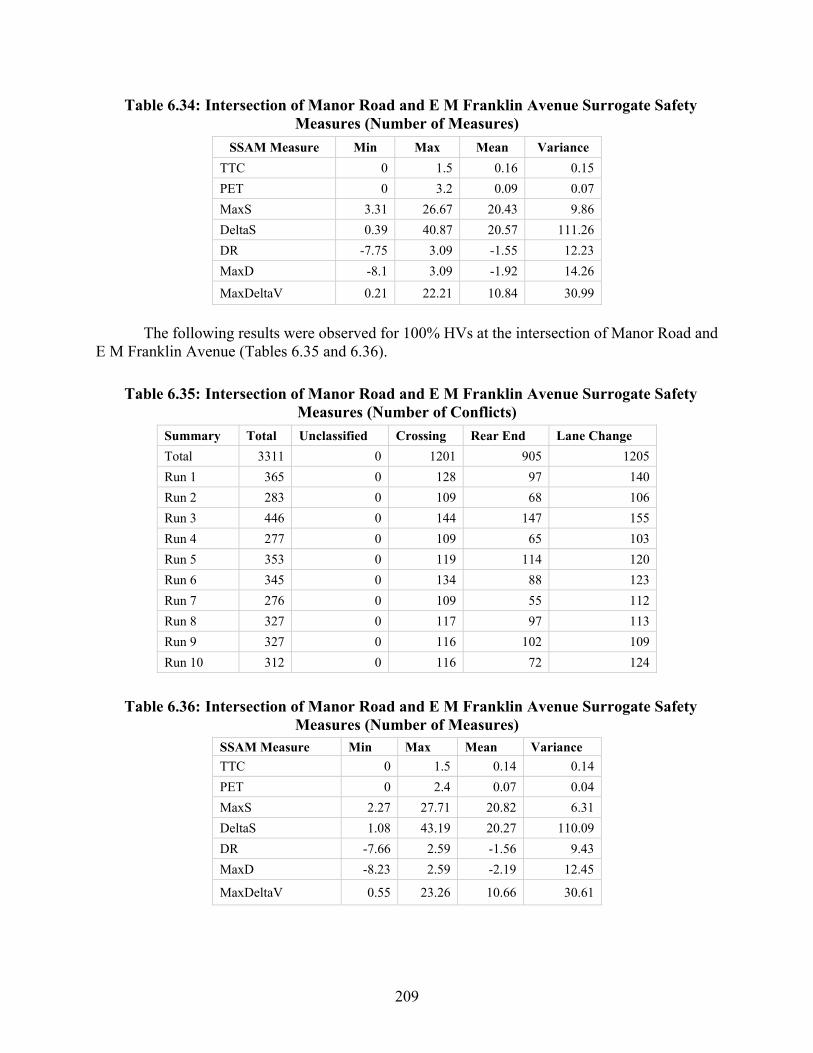
209

Table 6.34: Intersection of Manor Road and E M Franklin Avenue Surrogate Safety Measures (Number of Measures)

SSAM Measure Min Max Mean Variance

TTC 0 1.5 0.16 0.15

PET 0 3.2 0.09 0.07

MaxS 3.31 26.67 20.43 9.86

DeltaS 0.39 40.87 20.57 111.26

DR -7.75 3.09 -1.55 12.23

MaxD -8.1 3.09 -1.92 14.26

MaxDeltaV 0.21 22.21 10.84 30.99

The following results were observed for 100% HVs at the intersection of Manor Road and

E M Franklin Avenue (Tables 6.35 and 6.36).

Table 6.35: Intersection of Manor Road and E M Franklin Avenue Surrogate Safety Measures (Number of Conflicts)

Summary Total Unclassified Crossing Rear End Lane Change

Total 3311 0 1201 905 1205

Run 1 365 0 128 97 140

Run 2 283 0 109 68 106

Run 3 446 0 144 147 155

Run 4 277 0 109 65 103

Run 5 353 0 119 114 120

Run 6 345 0 134 88 123

Run 7 276 0 109 55 112

Run 8 327 0 117 97 113

Run 9 327 0 116 102 109

Run 10 312 0 116 72 124

Table 6.36: Intersection of Manor Road and E M Franklin Avenue Surrogate Safety Measures (Number of Measures)

SSAM Measure Min Max Mean Variance

TTC 0 1.5 0.14 0.14

PET 0 2.4 0.07 0.04

MaxS 2.27 27.71 20.82 6.31

DeltaS 1.08 43.19 20.27 110.09

DR -7.66 2.59 -1.56 9.43

MaxD -8.23 2.59 -2.19 12.45

MaxDeltaV 0.55 23.26 10.66 30.61

210

The following results were observed for 50% HVs and 50% AVs at the intersection of Manor Road and E M Franklin Avenue (Tables 6.37 and 6.38).

Table 6.37: Intersection of Manor Road and E M Franklin Avenue Surrogate Safety Measures (Number of Conflicts)

Summary Total Unclassified Crossing Rear End Lane Change

Total 3549 0 1223 960 1366

Run 1 372 0 121 100 151

Run 2 296 0 104 76 116

Run 3 392 0 128 123 141

Run 4 335 0 127 75 133

Run 5 344 0 116 83 145

Run 6 384 0 138 94 152

Run 7 307 0 113 79 115

Run 8 378 0 133 112 133

Run 9 366 0 119 108 139

Run 10 375 0 124 110 141

Table 6.38: Intersection of Manor Road and E M Franklin Avenue Surrogate Safety Measures (Number of Measures)

SSAM Measure Min Max Mean Variance

TTC 0 1.5 0.13 0.13

PET 0 2.6 0.07 0.04

MaxS 3 27.71 20.51 7.41

DeltaS 0.87 41.16 19.66 104.76

DR -8.24 2.52 -1.68 10.1

MaxD -8.36 2.52 -2.38 13.3

MaxDeltaV 0.44 22.14 10.35 29.04

In summary, the VisSim simulations and the subsequent SSAM analyses suggest that AVs

may be safer on selected networks in comparison with HVs. It was observed that the number of crashes and their severity decreases as the share of AVs in the traffic stream rises. The results were not completely consistent in trend. Certain measures, such as DeltaS and MaxDeltaV, showed unexpected patterns for some conditions. These discrepancies were minor, however, and no major anomalies were encountered. The reason for the observed discrepancies could be the difference in the behavior of AVs for different road networks; the AV and HV model used for this analysis may also require better calibration to provide more realistic results.

211

Chapter 7. MOVES Emissions Modeling

7.1 Introduction

In addition to affecting human mobility and safety, connected autonomous vehicles (CAVs) are also expected to impact emissions, air quality, and energy use. Many elements of vehicular and fuel technologies are associated with the energy use and emissions, such as vehicle weights (Greene 2008; Ford 2012; Chapin et al. 2013; MacKenzie et al. 2014), fuel efficiencies and alternative fuels (Chapin et al. 2013; Liu et al. 2015; Reiter and Kockelman 2016), and engine technologies (Paul et al. 2011; Folsom 2012; Bansal et al. 2016; Reiter and Kockelman 2016). CAVs are anticipated to be lighter than existing human-driven vehicles (HVs) (Chapin et al. 2013; Anderson et al. 2014), and powered by alternative fuels or electricity (Chen and Kockelman 2015; Chen et al. 2016) and more efficient engines (Anderson et al. 2014). CAV operational features are also likely to affect the energy used and emissions generated. Anderson et al. (2014) pointed out that CAVs would likely have fewer stop-and-go movements, given the connectivity of vehicle-to-vehicle (V2V) and vehicle-to-infrastructure (V2I), resulting in lower levels of fuel consumption and emissions. Fagnant and Kockelman (2014) simulated a fleet of shared autonomous vehicles (SAVs) to serve travelers in an idealized small city and estimated that each SAV might replace 11 HVs while increasing total vehicle-miles traveled (VMT)—due to empty-vehicle driving (to reach the next trip-maker). However, a high rate of SAV warm-starts (73% of trips began with a warm engine) and the use of smaller vehicles (as well as a need for fewer parking spaces, and their embodied emissions) led to overall estimates of lower emissions. Fagnant and Kockelman (2014) estimated that such SAV fleets could deliver an energy savings of 12%, along with a 5.6% reduction in greenhouse gas (GHG) emissions, relative to privately owned and operated HVs. AV platooning can also be expected to be associated with higher fuel efficiency and lower emission rates (Alam et al. 2010; Tsugawa 2014). Wu et al. (2014) discussed the sustainability benefits of vehicle automation at signalized intersections. Their results indicated 5 to 7% reductions in energy use and GHG emissions, up to 7% reductions in hydrocarbon (HC) emissions, and 15 to 22% reductions in carbon monoxide (CO) emissions. Wadud et al. (2016) expect greater energy savings and emissions reductions at higher levels of vehicle automation. Chen et al. (2016) estimated the energy and emissions benefits from an automated-vehicle-based personal rapid transit system and revealed approximately 30% energy saving and reductions in GHG emissions.

CAV technologies are also expected to improve fuel economy and reduce emissions per mile driven through more automated and optimized driving, thanks to more gradual acceleration and deceleration in driving cycles. A driving cycle is often represented as a vehicle’s speed profile versus time. Figure 7.1 presents a driving cycle designed by the Environmental Protection Agency (EPA) to represent highway driving conditions under 60 mph. In using HVs, driving patterns with gradual acceleration and deceleration are often referred to as “eco-driving” profiles (see, e.g., Anderson et al. 2014; Barth and Boriboonsomsin 2009; Chapin et al. 2013). Barth and Boriboonsomsin (2009) expect approximately 10 to 20% fuel savings and GHG emissions reductions, from humans driving conventional vehicles more thoughtfully, to reduce their energy use. Given the precision of fully automated driving, CAV driving profiles are likely to be much more fuel-efficient or at least smoother than human-controlled eco-driving profiles. Mersky and Samaras (2016) simulated the automated following driving cycles to estimate the changes in energy use and found up to 10% energy savings. This paper estimates the energy and emissions impacts of CAVs, by presuming that CAVs can (and ultimately will be programmed to) deliver

212

smooth driving cycles or engine loading profiles, effectively practicing Eco-Autonomous Driving (EAD).

Source: EPA, 2013

Figure 7.1: An EPA Driving Cycle for Conventional Vehicles on Highway Driving Conditions

To simulate the EAD profile, this study employed two types of existing HV driving cycles: 1) EPA driving cycles used to test for compliance with Corporate Average Fuel Economy (CAFE) standards for light-duty vehicles (EPA 2012), and 2) Austin-specific driving schedules developed by the Texas A&M Transportation Institute (TTI) to reflect local driving patterns of light-duty vehicles (Farzaneh et al. 2014). The EAD profiles were simulated by smoothing the existing driving cycles, given the anticipation that CAV driving profiles will contain fewer extreme driving events (like hard accelerations, sudden braking, and sharp or quick turns) than HV cycles. Then, this study used the US EPA’s Motor Vehicle Emission Simulator (MOVES) to estimate emission rates (in grams per mile traveled) for various pollutants, including volatile organic compounds (VOC), fine particulate matter (PM2.5), carbon monoxide (CO), nitrogen oxides (NOx), sulfur dioxide (SO2) and carbon dioxide (CO2), based on the EAD profiles and HV cycles.

MOVES is the EPA’s regulatory simulator for estimating on-road emissions from conventional vehicles such as passenger cars, buses, and trucks. It is used by planning organizations for project conformity analyses that are required for state implementation plans (SIPs), as well as for environmental analyses that gauge the impacts of potential transport planning decisions (EPA 2014, 2015). The EPA and state environmental agencies have developed a database that provides basic emissions parameters for counties across the U.S. (EPA 2015). Though this database is continually updated to provide the most accurate parameters for a given area, the EPA recommends that local data be developed and inserted into the MOVES simulator to provide the best estimate of on-road emissions at the project area, which Farzaneh et al. (2014) did for several Texas cities.

In this report, CAV emissions impacts are limited to differences in basic driving profiles, as elected by independent CAVs driving at the same time in the same locations, with the same traffic control strategies and traffic variations that HVs face. In reality, many other CAV technologies and applications (like cooperative intersection coordination systems, platooning and coordinated adaptive cruise control) should also help save fuel and reduce emissions, but these are not evaluated in this paper. In addition, many factors that may affect the fuel consumption and

Spe

ed (

mph

)

Time (seconds)

213

emissions of vehicles, such as vehicle size and road grade (Boriboonsomsin and Barth 2009) are not discussed here.

7.2 Envisioning Eco-Self-Driving Cycles of Autonomous Vehicles

This section presents the Eco-Self-Driving (ESD) cycles that are envisioned for CAVs based on existing HV driving cycles. The HV driving cycle data used in this task include EPA driving cycles that are used for the Corporate Average Fuel Economy (CAFE) for light-duty vehicles (EPA 2012), and Texas-specific driving schedules (Farzaneh, et al. 2014). ESD cycles are expected to be smoother than HV cycles, given the advances in CAVs as relative to HVs.

7.2.1 Smoothing Method

Many methods can be used to smooth the driving cycles, such as moving average, local polynomial regression, kernel density estimation, and smoothing splines (Simonoff 2012). Most data smoothing efforts are designed to impute missing data points or smooth out noise. In contrast, this study envisions CAV’s ESD cycles by smoothing the existing HV cycles. There are two main concerns with the smoothed driving cycles:

1. CAV’s ESD profiles should have far fewer extreme driving events—like hard accelerations and sudden braking, as compared to HV cycles. Intelligent and CV-informed vehicles should be able to anticipate several seconds of downstream driving conditions, making timelier decisions and ultimately smoother responses to evolving traffic conditions. In such cases, a higher extent of smoothing (like a wider smoothing window) can be expected.

2. However, CAV’s movements on road are influenced by other vehicles (when there is no free-flow and HVs are still on road) and the traffic control devices (like intersection signals and signs). Therefore, at the early stage of introducing CAVs on road, the CAV profiles may be somehow similar to HV cycles from a microscopic perspective. In other words, the time-distance diagrams of both CAV (smoothed) and HV (unsmoothed) driving profiles should generally be similar to each other, to ensure that smoothed cycles do not make travelers late for meetings, late to green lights, or unyielding to (and thus colliding with) driveway-entering vehicles and the like. And the extent of smoothing (or level of smoothness) should not be extreme. This assumption implies largely unchanged driving patterns, from a macroscopic perspective. However, CAV technologies are likely to eventually impact such patterns, as adoption and use rates rise; cooperative intersection management and smart CAV routing decisions will shorten travel times, everything else constant, but added VMT may make travel more congested. Such changes in load profiles are not examined here.

The first concern is about small curvatures of the cycles and the second concern is about

the great similarities between smoothed and original cycles (i.e., small mean squared errors or MSE). In order to approximate this “balance” between these two concerns, the method of smoothing spline was employed in this study. The smoothing process is to minimize the objective

function: argmin ∑ ( − ( )) + ( ( ))

214

where, the first term is the mean squared errors ( = the speed value of y at ith data point in an original driving cycle, i = 1, 2, …, n; ( ) = the predicted value of m at ith data point in a smoothed driving cycle); ( ) = the second derivative of m with respect to x, i.e., the curvature of m at x; = the smoothness factor to penalize mean squared errors. As → + ∞, the MSE is not a concern and there is only a linear function resulted from the smoothing process. In contrast, as → 0, the curvature is negligible and remains the same as un-smoothed. To address both these ideas and the two objectives or complexities listed above, an appropriate smoothness factor was chosen to construct smoothing cycles.

To determine the most appropriate smoothness factor, various values were tested, as shown in Figure 7.2. The larger smoothness factor = 0.8 is associated with a smoother cycle, compared with smaller smoothness factors, the time-distance diagram of the smoothed cycle significantly deviates from the original cycle.

To better appreciate the effects of the chosen λ, the distributions of the smoothed and original cycles’ accelerations and decelerations were also compared. Figure 7.3 presents the distributions of acceleration/deceleration values before smoothing (when λ=0) and after the smoothing. For comparison, typical distributions of acceleration/deceleration are shown in the figure as well, indicated by means (solid line) and means plus one standard deviation (dashed lines). The means and standard deviations were calculated for specific speed ranges (with bin width = 0.5 mph) using large-scale trajectory data from the Austin region.

The trajectory data were obtained from the Transportation Secure Data Center (TSDC) of the National Renewable Energy Laboratory (NREL) (TSDC 2014). The data were originally collected in TTI’s 2006 Austin/San Antonio GPS-Enhanced Household Travel Surveys. This study extracted 241 hours of second-by-second driving speed records collected from 231 vehicles in Austin, Texas in 2005–2006. (More details about the calculation of distributions of acceleration/deceleration along speeds can be found in Wang et al. 2015. Note that the distributions can vary from one region to another). Figure 7.3 shows how, with a high smoothness factor (λ=0.8), the accelerations/decelerations are close to zero across speeds. To ensure that AV cycles remain similar to existing HV cycles (in order stop at red lights, and slow when vehicles merge in front of a CAV), this study chose λ=0.22999 as the smoothing factor, since this value allows most acceleration/deceleration data points to lay within the mean + one standard deviation of the typical distributions in the Austin region. In the study by Wang et al. (2015), the acceleration/deceleration data points were regarded as extreme driving events for falling beyond the mean-value lines plus one standard deviation, reflecting the unpredictable maneuvers of HVs. As CAVs become more common in traffic streams, such unpredictable maneuvers are likely to fall dramatically (thanks to inter-vehicle communications).

215

Figure 7.2: Driving Cycle Example (Smoothed CAV Cycle vs. Original HV Cycle)

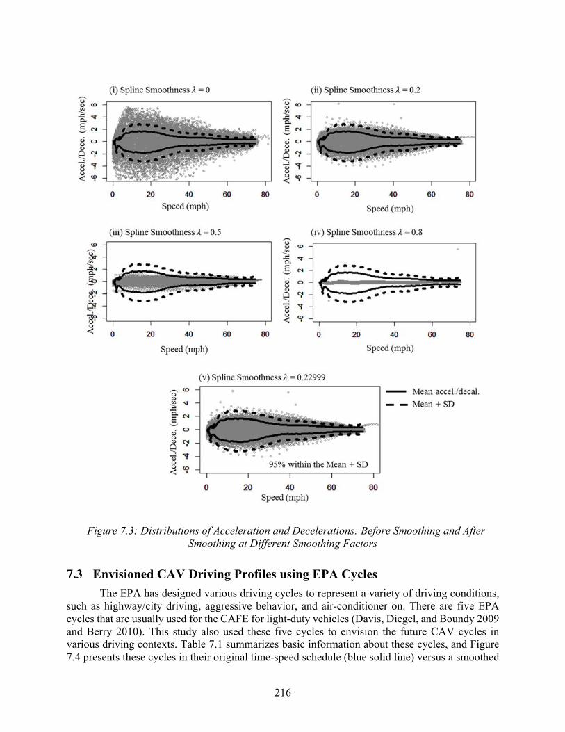
216

Figure 7.3: Distributions of Acceleration and Decelerations: Before Smoothing and After

Smoothing at Different Smoothing Factors

7.3 Envisioned CAV Driving Profiles using EPA Cycles

The EPA has designed various driving cycles to represent a variety of driving conditions, such as highway/city driving, aggressive behavior, and air-conditioner on. There are five EPA cycles that are usually used for the CAFE for light-duty vehicles (Davis, Diegel, and Boundy 2009 and Berry 2010). This study also used these five cycles to envision the future CAV cycles in various driving contexts. Table 7.1 summarizes basic information about these cycles, and Figure 7.4 presents these cycles in their original time-speed schedule (blue solid line) versus a smoothed

217

time-speed profile (red dashed line). The smoothed cycles are envisioned to be the driving profiles for CAVs operating in the trip conditions listed in Table 7.1.

Table 7.1: EPA Cycles

EPA Cycle Represented

Trip Information

Max. Speed

Avg. Speed

Max. Acceleration

Simulated Distance

Duration Test

Temp

FTP (Federal Test Procedure)

Low speeds in stop-and-

go urban traffic

56 mph 21.2 mph 3.3 mph/sec 11 mi. 31.2 min. 68°F–86°F

HWFET (Highway

Fuel Economy Driving

Schedule)

Free-flow traffic at highway speeds

60 mph 48.3 mph 3.2 mph/sec 10.3 mi. 12.75 min. 68°F–86°F

US06 (Supplemental

FT)

Higher speeds; harder

acceleration & braking

80 mph 48.4 mph 8.46 mph/sec 8 mi. 9.9 min. 68°F–86°F

SC03 (Supplemental

FTP)

A/C use under hot ambient

conditions

54.8 mph

21.2 mph 5.1 mph/sec 3.6 mi. 9.9 min. 95°F

UDDS (Urban

Dynamometer Driving

Schedule)

City test w/ colder

outside temp. 56 mph 21.2 mph 3.3 mph/sec 11 mi. 31.2 min. 20°F

Source: EPA 2013

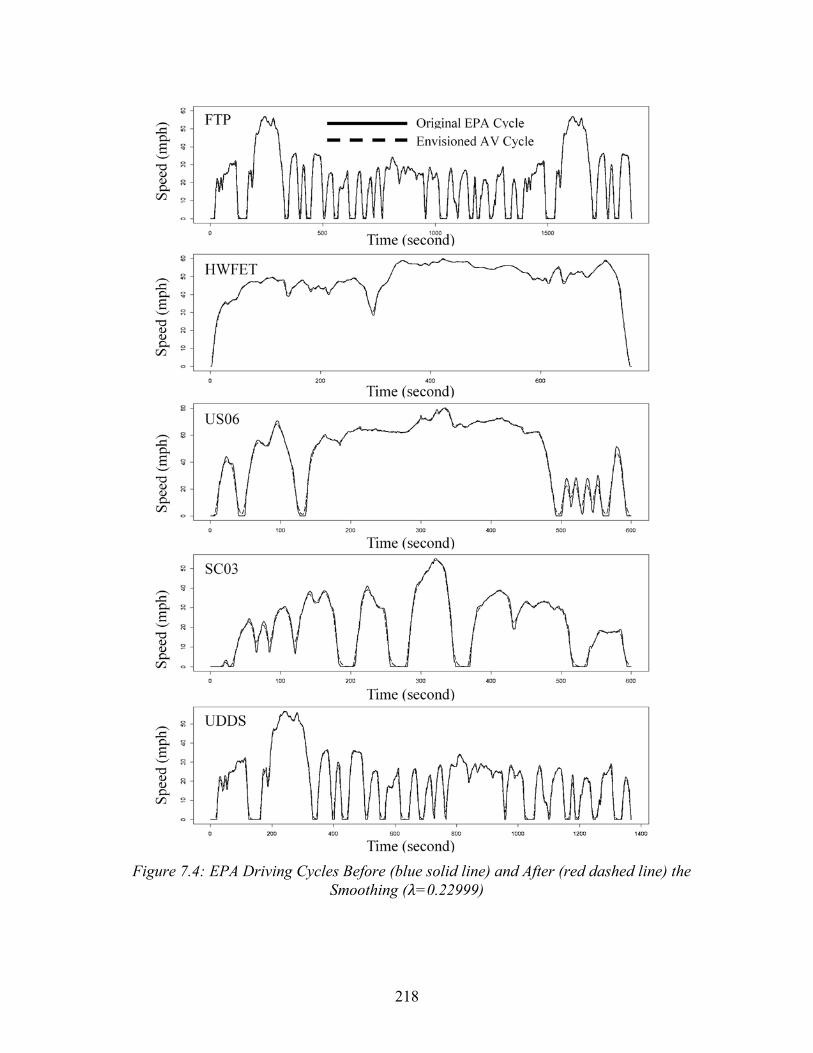
218

Figure 7.4: EPA Driving Cycles Before (blue solid line) and After (red dashed line) the

Smoothing ( =0.22999)

219

7.4 Envisioned CAV Driving Profiles using Austin Cycles

EPA’s cycles represent national representative drive schedules. Using a single set of representative driving cycles for fuel consumption and emissions estimates ensures comparable results across vehicle types, fuel types, manufacturers and many other factors. For this task, the researchers sought Austin-specific driving cycles, extracting them from the Database of Texas-Specific Vehicle Activity Profiles for Use with MOVES (Farzaneh, et al. 2014). Note that these extracted cycles do not represent a complete automobile trip, but rather a specific type of road link (or a road segment). These links may be combined to create a complete cycle. In this task, the analysis is conducted at link level. In future analysis these links may be summed at different weights according to their proportions in the Austin road network.

In total, 36 links were extracted from the database, covering two types of light-duty vehicles (passenger car and light-duty truck), two types of roadways (urban restricted and unrestricted road), and nine link-level average speed bins. Using the smoothing method introduced above, the links’ driving cycles were smoothed to envision the driving profiles of CAVs running in the Austin region. Given the large number of links, the original and smoothed driving profiles are not shown in this report. Instead, Figure 7.3 presents the distributions of acceleration/deceleration (i) before and (ii) after the smoothing. Figure 7.3(v) gives the distributions of acceleration/deceleration in envisioned CAV driving profiles.

7.5 Preparing Data Inputs for MOVES

7.5.1 Configuring MOVES for Emission Estimations

MOVES is the EPA’s regulatory simulator for estimating on-road emissions from conventional vehicles, such as passenger cars, buses, and trucks. It is used by planning organizations for project conformity analyses that are required for state implementation plans (SIPs). MOVES is also used to gauge the air quality impacts of potential transport planning decisions. The EPA and other state agencies have developed a database that provides basic emissions parameters for counties across the U.S. Though this database is continually updated to provide the most accurate parameters for a given area, the EPA recommends that local data be developed and inserted into the MOVES simulator to provide the best estimate of on-road emissions at the project area, which is what Farzaneh et al. (2014) did for several Texas regions.

Several studies have employed MOVES to estimate on-road emissions. Instead of using real data to estimate travel times, queue length, and other parameters, microsimulation data can provide the needed MOVES inputs. This method was employed by Xie et al. (2012) to estimate emissions on a freeway segment in Greenville, South Carolina. The researchers used PARAMIC to simulate the freeway operations and outputs were used in MOVES for emissions modeling. Xie et al. modified the fuel table to estimate the environmental benefits of using alternative fuels. Their results showed alternative fuels changed emissions rates as expected, but the scope of their study was limited to one freeway segment.

Another emissions study was performed by Abou-Senna and Radwan (2013). This study employed VisSim to produce driving patterns along a single highway corridor. The researchers wanted to look at how traffic volume, vehicle speed, grade, and temperature affected CO2 emission rates. The vehicles in their VisSim model were categorized into operating bins based on the vehicle specific power (VSP) of the cars in the microscopic simulation. The magnitude of a car’s VSP is used to estimate the severity of the emissions rates of that particular vehicle. Their results produced

220

another example of data transferability between a traffic simulator and MOVES, and reconfirmed that increasing factors like grade and traffic volume on a link lead to higher emission rates.

Amirjamshidi and Roorda (2015) also developed simulated driving cycles for the Toronto Waterfront area using a microsimulator. Their simulation program produced sets of micro-trips, which are the periods of driving by a vehicle between two successive idles, and then randomly selected micro-trips to piece together and form drive cycles. The researchers chose to develop drive cycles for light, medium, and heavy-duty trucks in the AM peak. These cycles were inserted into MOVES version 2010b to produce CO2 emission rates.

Several other studies have used microsimulation programs to develop drive cycles for a particular project area. However, all of these microsimulations have modeled conventional vehicles only. Because of the lack of readily available microsimulation data representing CAV driving behavior, the most optimal and feasible method of predicting CAV emission rates is by statistical smoothing of driving cycles used to model HV driving behavior. This is based on the assumption that CAVs will be optimized in a way in which their movement will minimize the erratic acceleration behavior associated with higher emission rates. Other studies have not employed this technique to predict CAV emission rates, and this would be an important contribution to HV/CAV planning research.

To run a project-scale analysis in MOVES, the model must be configured with the desired parameters. The MOVES model output is called a RunSpec. The parameters that must be specified are listed below:

1) Scale – this study employed a project-scale domain. This is generally smaller than a county- or national-scale analysis. This task is based on the EPA driving cycles and the Austin link-based cycles (before and after the smoothing). Therefore, this task is, to be specific, to estimate the emissions on several road segments or combinations of road segments on which the vehicles run in EPA cycles or Austin link-based cycles.

2) Time Span – because the scale is set at the project level, MOVES allows the RunSpec to simulate only one hour of emissions production at a time. The RunSpec program was processed individually for several different hours to estimate emissions for longer than one hour.

3) Geographic Bounds – the county where the project is located is selected (Travis County for this analysis).

4) Vehicles/Equipment – the types of vehicles that emissions will be produced from in the simulation are specified with this parameter. Additionally, the fuels these vehicles use are also specified. For this project, passenger cars and light-duty trucks powered by diesel fuel, ethanol (E-85), and gasoline were considered. Fuel source distribution is consistent with the default values in MOVES.

5) Road Type – the five available road types to be modeled in MOVES are off-network, rural roads, and urban roads. Urban and rural roads are classified as having either restricted or unrestricted access. Only urban roads were considered in this analysis.

6) Pollutants and Processes – these are the pollutants and emissions processes being modeled by MOVES. The user selects the combinations of pollutants and the process to model for his or her project. MOVES can model emission of pollutants such as VOC, CO2, nitrous oxides, hydrocarbons, and particulate matter (PM) with mean diameter of 2.5 μm (PM2.5), and PM with mean diameter of 10 μm (PM10).

221

7.5.2 Data Inputs for MOVES

After finishing the configuration of the MOVES model, the user enters project-specific data into the Project Data Manager. There are up to 13 inputs that the user can specify to customize the MOVES model for a project. The inputs specified for this project are listed and described below:

1) Links – the user specifies the road type, length, volume, average speed, and grade of each link being modeled in the project analysis. The road type, length, and average speed for each link considered was provided in the Texas drive cycle database referenced earlier. The grades of all roads were considered as flat. Though this is a very simplistic assumption, analyzing the emissions impacts of smoothing cycles can still be performed effectively because the input parameters remain the same for both unsmoothed and smoother driving cycles. Only urban restricted and urban unrestricted roads were considered in this analysis to minimize MOVES run times. The volume of the link, which is the total traffic volume in one hour, was considered to be 145,000 vehicles for urban restricted roads and 10,000 for all urban unrestricted roads included in the analysis (averaged according to TxDOT highway system statistics). Since link volumes are not readily available in a database for each link on a network, a conservative estimate was used for both urban restricted roads and urban unrestricted roads.

2) Link Source Types – each link considered must have the vehicle mix specified. Only light vehicles were considered in this analysis due the lack of available data highlighting the actual vehicle mixes in this analysis.

3) Link Drive Schedules – the speed versus time profiles (drive cycles) extracted from the Texas drive cycle database were used as the model of driving behavior for vehicles in the project area.

4) Age Distribution – The proportions of cars within age ranges are specified in MOVES. The program includes default proportions for each year, and this study used default values due to the lack of available local information on age distribution.

5) Fuel – The types of fuels used by vehicles on the network must be specified. Many analyses rely on default fuel databases maintained by MOVES, and this study took the same approach.

6) Off-Network – the user specifies the start fraction, which is the average fraction of vehicle population that has started during the hour. The extended idle fraction is also specified when trucks are considered. Since only light vehicles were included in this analysis, no extended idle fraction was specified.

7) Meteorology Data – the average temperature and humidity at a given time and location is provided by MOVES. The EPA provides this information inside of MOVES for each county in the U.S.

8) Truck Hoteling – if heavy-duty trucks are included in the analysis, the fraction of hours when trucks are idling roadside, or “-hoteling” should be specified. This was not relevant here because only the active operation of light-duty CAVs were simulated.

222

7.6 CAV Emissions Impacts

This section presents emissions estimates based on smoothed driving cycles (for light-duty CAVs), using MOVES, as compared to original, HV driving schedules. Results using the US EPA’s national driving cycles are presented first, followed by some Austin-specific driving cycle results.

7.6.1 Emission Estimates using EPA Cycles

The emission rates of a specific type of pollutants were estimated for light-duty passenger vehicles. The HV emission estimations were based on the original EPA schedules and the CAV emissions were estimated according to the corresponding smoothed EPA schedules.

Figure 7.5 presents the estimates of volatile organic compounds (VOC) emissions. The estimates are generally reasonable. For example, 1) the SC03 cycle with air-conditioning on in high temperature of 95°F and FTP cycle with frequent acceleration and brake events at low speeds lead to the high emission rates in both gasoline and diesel vehicles; and 2) the HWFET cycle representing free-flow freeway traffic is associated with the least emission rates, with other factors held constant. CAV emission levels are expected to be lower than those of HVs. Among both gasoline and diesel passenger vehicles, all five cycles are estimated to have lower VOC emission rates after the spline smoothing. Noticeably, the HWFET cycle is associated with the smallest emissions reductions, perhaps because this cycle does not contain many hard brakes and accelerations. The US06 cycle is linked with greatest emissions reductions (6.25% to 6.65%), as the original US06 cycle contains many rapid acceleration and hard-braking events that may occur only rarely in CAV operations. FTP cycle is associated with the second greatest reductions (4.99% to 5.23%) in VOC emissions.

Figure 7.5: Emission Estimates for VOC

Figure 7.6 shows estimated emissions of particulate matters (PM), carbon monoxide (CO), nitrogen oxides (NOx), and carbon dioxide (CO2). Variations are found in these emission species. US06 cycle leads to greater emission rates than FTP and HWFET cycles for emissions of PM 2.5 and CO, owing to the hard brakes and accelerations in US06 cycle. UDDS SC03 cycles are found to have the greatest emission rate of PM2.5, and CO, respectively, for gasoline vehicles. The reason may be related to the testing temperature: UDDS was tested at extreme cold temperature, 20°F, and SC03 cycle was to simulate the driving in hot weather, 95°F. For emissions of NOx, US06 cycle leads to greatest emission rates among both gasoline and diesel vehicles. FTP cycle has

223

relatively great CO2 emission rates, which may be related to the low-speed driving, and frequent acceleration or brake events.

Regarding the emission reductions from HVs and CAVs, FTP and UDDS cycles seem to have great reductions (> 10%) in emissions of PM 2.5 and NOx. US06 cycle is expected to have great reductions (around 7%) in emissions of CO. Again, HWFET cycle with least hard brake and acceleration events is related to the smallest reductions across all emission species.

Overall, smoothed EPA cycles were associated with lower emission rates, indicating that CAVs are likely to be more environmentally friendly than HVs. However, these reductions are not guaranteed, and vary according to emission types, fuel types, and driving contexts.

224

Figure 7.6: Emission Estimates for PM2.5, CO, NOx, and CO2

225

7.6.2 Emissions Estimates using Austin-area Cycles

The original and smoothed Austin cycles as obtained from TTI researchers (Farzaneh 2014) were entered into the MOVES program to estimate the emissions of current HV fleets and future CAV fleets. To make the results comparable, all configurations and inputs in MOVES except the inputs of driving schedules were identical for HV and CAV emission estimates. The emissions were estimated in 36 Austin-specific cycles that represent the local driving patterns.

Given the variety of pollutant types, fuel types, vehicle types, various cycles, etc., simple regression models were constructed to present and explain the results. The correlates of emissions reductions for a specific pollutant were explored. The response or dependent variable is the percentage reduction in any specific pollutant species. Explanatory or independent variables (X1, X2, etc.) include fuel type, vehicle type, temperature, and link-level average speed values. All explanatory variables, except link-level average speed values are indicators (X = 0 or 1) variables, and just two ambient temperature conditions (cold, 40°F in January, and warm, 75°F in September) were simulated. Table 7.2 shows the descriptive statistics of variables in the regression models. The models for different pollutants had exactly the same descriptive statistics.

Table 7.2: Summary Statistics of Emissions-Related Variables

(i) Explanatory Variables

Variable Mean or Proportion S.D. or Freq. Min Max

Vehicle Type Passenger Car 50% 216 0 1

Light-Duty Truck 50% 216 0 1

Fuel Type

Gasoline 33% 144 0 1

Diesel 33% 144 0 1

Ethanol 33% 144 0 1

Temperature Cold 50% 216 0 1

Hot 50% 216 0 1

Link Mean Speed (mph) 30.18 21 2.5 69.5

(ii) Emission Reductions

Emission Species Average Drop S.D. Min Max

Volatile Organic Compounds - VOC 10.89% 9.09% -4.56% 30.77%

Fine Particulate Matter - PM2.5 19.09% 17.31% -23.81% 59.66%

Carbon Monoxide - CO 13.23% 16.50% -16.93% 40.04%

Nitrogen Oxides - NOx 15.51% 11.50% -7.41% 38.63%

Sulfur Dioxide – SO2 6.55% 5.45% -4.12% 16.77%

Carbon Dioxide - CO2 6.55% 5.45% -4.11% 16.76%

Note: all variables except Link Mean Speed and Emission Reduction are indicator variables. No. of observations = 432 for each emission type.

Figure 7.7 presents the distributions of percent reductions (Y) in emissions of VOC, PM2.5, CO, NOx, SO2, and CO2. The positive percentages indicate the emissions reductions from HV to CAV cycles. The magnitudes of percent reductions are generally consistent with the estimates from EPA cycles. In most cases, the estimated emissions decreased during the shift from HV to CAV cycles (i.e., positive percentages). The mean emission reductions are 10.89% for VOC, 19.09% for PM2.5, 13.23% for CO, 15.51% for NOx, and 6.55% for SO2 and CO2.

226

Figure 7.7: Distributions of Emissions Reductions (in percentages) of VOC, PM2.5, CO, NOx,

SO2, and CO2

Table 7.3 delivers the regression models, showing the correlates of emission reductions (from HV to CAV EAD cycles) with the factors shown in Table 7.2. The coefficients refer to the changes in emission reductions (%) from HV to CAV cycles, with one unit change in explanatory variables, when controlling for other variables. The findings from the models include the following:

• VOC: Greater reductions in VOC emissions are expected for passenger cars, 1.925 percentage points more than for passenger trucks. Diesel vehicles showed smaller emission reductions, 4.636 percentage points less than vehicles powered by ethanol. Higher average link speeds lead to greater reductions in VOC emissions, while a one-unit increase in speeds results in a reduction in VOC of 0.273 percentage points less.

• PM2.5: Gasoline vehicle are associated with a greater reduction (4.367 percentage points more) in emissions of PM2.5, and diesel vehicle are linked with a smaller reduction (8.307 percentage points less), as relative to the vehicles powered by ethanol. The road links with higher average speeds are expected to have a greater emission reduction. A one-unit increase (1 mph) in average speed corresponds to a 0.302 percentage point reduction in PM2.5 emissions.

227

• CO: Passenger cars are related to greater CO emission reductions (1.655 percentage point more) when moving from HV to CAV cycles, as relative to passenger trucks. Diesel vehicles demonstrated smaller emission reductions, 2.131 percentage points less than vehicles powered by ethanol. Higher average link speeds are expected to result in a greater reduction in CO emissions. The regression shows that a one-unit increase in average link speed results in a 0.505 percentage points greater emission reduction in CO.

• NOx: Passenger cars demonstrated greater NOx emission reductions from the HV to CAV cycles, 1.363 percentage points more than passenger trucks. Diesel vehicles showed smaller emission reductions, 4.042 percentage points less than vehicles powered by ethanol. Higher average link speeds are expected to result in a lower reduction in NOx emissions, while a one-unit increase in speeds results in a reduction in NOx of 0.048 percentage points less.

• SO2 and CO2: These two types of emissions were found to have similar correlates of emission reductions. Only the link average speed has a significant correlation with these emission reductions. Higher link average speeds are expected to result in a lower reduction in SO2 and CO2 emissions. A one-unit increase in speeds results in a reduction in SO2 and CO2 emissions of 0.069 percentage points less.

228

Table 7.3: Regression Results for Y = % Emission Reductions, as a Function of Vehicle, Fuel Type, Starting Engine Temperature, and Average Speed

Emission Species Variable β Std Error p-value R-Square

Volatile Organic Compounds

(VOC)

Constant 2.641 ** 5.74 <.0001 0.643

Passenger Car (base: Passenger Truck) 1.925 ** 7.33 <.0001

Gasoline (base: Ethanol) -0.588 -1.58 0.1146

Diesel (base: Ethanol) -4.636 ** -12.47 <.0001

Cold (base: Hot) -0.188 -0.72 0.4737

Link Mean Speed (mph) 0.273 ** 21.81 <.0001

Fine Particulate Matter (PM2.5)

Constant 9.983 ** 7.87 <.0001 0.253

Passenger Car (base: Passenger Truck) -0.862 -1.19 0.2342

Gasoline (base: Ethanol) 4.367 ** 4.27 <.0001

Diesel (base: Ethanol) -8.307 ** -8.12 <.0001

Cold (base: Hot) 0.550 0.76 0.4477

Link Mean Speed (mph) 0.302 ** 8.75 <.0001

Carbon Monoxide (CO)

Constant -2.011 ** -2.95 0.0034 0.646

Passenger Car (base: Passenger Truck) 1.655 ** 4.25 <.0001

Gasoline (base: Ethanol) 0.038 0.07 0.9455

Diesel (base: Ethanol) -2.131 ** -3.87 0.0001

Cold (base: Hot) 0.080 0.21 0.8373

Link Mean Speed (mph) 0.505 ** 27.20 <.0001

Nitrogen Oxides (NOx)

Constant 14.054 ** 15.21 <.0001 0.103

Passenger Car (base: Passenger Truck) 1.363 * 2.59 0.0101

Gasoline (base: Ethanol) 0.116 0.16 0.8768

Diesel (base: Ethanol) -4.042 ** -5.42 <.0001

Cold (base: Hot) -0.275 -0.52 0.6017

Link Mean Speed (mph) 0.048 1.92 0.0555

Sulfur Dioxide (SO2)

Constant 4.480 ** 10.09 <.0001 0.076

Passenger Car (base: Passenger Truck) -0.392 -1.55 0.1225

Gasoline (base: Ethanol) -0.089 -0.25 0.8043

Diesel (base: Ethanol) 0.247 0.69 0.4903

Cold (base: Hot) 0.046 0.18 0.8562

Link Mean Speed (mph) 0.069 ** 5.69 <.0001

Carbon Dioxide (CO2)

Constant 4.479 ** 10.10 <.0001 0.076

Passenger Car (base: Passenger Truck) -0.391 -1.550 0.1231

Gasoline (base: Ethanol) -0.089 -0.250 0.804

Diesel (base: Ethanol) 0.248 0.690 0.4898

Cold (base: Hot) 0.046 0.180 0.8562

Link Mean Speed (mph) 0.069 ** 5.690 <.0001

Notes: ** = significant at 99% confidence level; * = significant at 95% confidence level.

229

7.7 Conclusions

This study seeks to anticipate some of the emission impacts of CAVs. CAV driving profiles are envisioned to be smoother than those of HVs, because CAVs are expected to be faster and more precise than human drivers, in terms of reaction times and maneuvering. Human drivers tend to create significant, frequent speed fluctuations (i.e., hard brakes and rapid accelerations) and have relatively long reaction times (e.g., 1.5 seconds). CAV technologies may rarely suffer from such fluctuations, allowing for smoother driving profiles, referred to here as Eco-Autonomous Driving (EAD) cycles. Hard braking and rapid acceleration events are associated with increased emissions, so, by smoothing HVs’ existing driving cycles, this work anticipates the emission benefits of CAVs.

National EPA cycles and Austin, Texas cycles were smoothed to obtain EAD emissions estimates using MOVES. Various emission species were considered here, including volatile organic compounds (VOC), fine particulate matter (PM2.5), carbon monoxide (CO), nitrogen oxides (NOx), sulfur dioxide (SO2), and carbon dioxide (CO2). Differences in HV versus CAV emissions estimates suggest valuable air quality from CAVs—assuming CAVs are driven no more than HVs would be.

The results from EPA cycles suggest that, in general, if HVs are replaced by AVs, greater emission benefits (up to 14% emission reductions) are anticipated in driving conditions where there are many hard acceleration and braking events, and for drivers with aggressive driving styles. The results from Austin cycles indicate the mean emission reductions are 10.89% for VOC, 19.09% for PM2.5, 13.23% for CO, 15.51% for NOx, and 6.55% for SO2 and CO2. Regression models revealed that passenger cars were found to be associated with lower emission reductions for VOC, PM2.5, CO, and NOx than passenger trucks. Diesel vehicles are linked with smaller emission reductions for these six types of emissions. The road links with higher average speeds have greater emission reductions for all emission species.

The results are solely based estimates from MOVES models. Other emission modeling tools, such as UC Riverside’s Comprehensive Modal Emissions Model (CMEM) (Scora and Barth 2006), may be employed in continuing efforts. At this point, the discussion of emission impacts of AVs is limited to the differences between the anticipated EAD profiles of CAVs and existing HV driving cycles. CAV profiles are envisioned to be smoother than HV cycles as compared to HV cycles. Other CAV-based technologies (like platooning of vehicles and CACC) may also save fuel and reduce emissions further.

230

Chapter 8. Anticipating the Regional Impacts of Connected and Automated Vehicle Travel

8.1 Introduction

Advanced transportation technologies, including connected vehicles (CVs), autonomous vehicles (AVs), and connected autonomous vehicles (CAVs), are undergoing development at an incredible speed. CAVs, which incorporate the advantages of CVs and AVs, have the potential to revolutionize the existing transportation system. One of the most significant benefits CAVs offer is a more pleasant travel experience for drivers, effectively reducing their value of travel time (VOTT). VOTT is defined as an individual’s willingness to pay to avoid another hour of travel. If an individual is able to both reduce stress and increase productivity while traveling, by becoming a passenger, rather than being forced to maintain focus on driving, his/her VOTT falls. This makes CAVs relatively attractive for current drivers, if not for current passengers. Moreover, many believe CAVs will eventually increase lane and roadway capacity by reacting faster to changes in preceding vehicles’ speeds and positions (via dedicated short-range communications [DSRC]; cameras; and light-detecting, radio-detecting, and ranging devices). Technical competence and rising confidence in CAV response times can lead to shorter following distances and headways between vehicles. Parking costs for CAVs may also fall, since AVs may be able to drop off their passengers and seek lower-cost parking elsewhere, or otherwise serve someone else’s trip-making needs (as in the case of shared autonomous vehicles [SAVs] or a privately owned CAV that is sent to another household member, for his/her trip).

SAVs are self-driving taxis, and so carry no driver costs. They can be “shared” as a rental fleet, and are likely to be quite cost competitive (as shown in Fagnant and Kockelman [2015], Chen et al. [2016], and Chen and Kockelman [2016]). Like taxis and buses, SAVs are a form of public transportation, and may be operated by public transit operators, such as a regional transit authority (e.g., CapMetro in Austin, TX), or private entities, like Lyft and Uber. Although SAV use may be costlier than buses, they can provide on-demand, door-to-door, and lower-occupant services. SAV users will benefit from more flexible schedules and pickup/dropoff locations, shorter waiting times, privacy, and possibly greater comfort.

This paper uses regional travel demand models to evaluate the system benefit brought by CAVs and SAVs. Travel demand models currently in use by most MPOs, DOTs, and their consultants are not set up to investigate the potential traffic impacts of CAVs and SAVs, though such vehicles are expected to be quite common over the next 20 to 30 years (Gulipalli and Kockelman 2015). Long-range city, regional, state, and national transportation planning activities should work to reflect the tremendous technological changes expected in the transportation sector, via self-driving vehicles (shared and private, passenger and freight, short-distance and long-distance). To this end, this study investigated how to best modify an existing, trip-based travel demand model in use in Texas, for the Austin region, to illustrate how MPOs and DOTs can start to account for CAVs’ travel demand and traffic impacts. Such behavioral changes also affect emissions and air quality, crash counts, noise levels, goods delivery and product prices (Fagnant and Kockelman [2015]). Given the uncertainty surrounding CAVs’ effects on behavior and travel costs, multiple model scenarios were developed to illuminate a range of possible transportation system futures for the Austin region. These scenarios vary the VOTTs, parking costs, headways, and other important travel choice factors. While these are initial rough estimates, they are still useful for transportation and urban system planners and decision-makers, when charting a course

231

for future investments and policies. The methods applied should also prove useful to travel demand modelers and planners. The following section discusses existing literature on the travel demand effects of AVs, CVs, CAVs, and SAVs, and several proposed frameworks to anticipate their transportation system impacts. Subsequent sections include key modeling assumptions (e.g., preference for using CAVs and SAVs due to the reduction of travel time disutility) and methods (e.g., modification of the existing models to consider the impacts of CAVs and SAVs) used here. This chapter then presents around 30 model scenarios to forecast the traffic impacts of CAVs and SAVs on Austin’s year 2020 networks, under different assumption scenarios. The chapter concludes with recommendations and suggestions for modeling extensions.

8.2 Literature Review

With the advent of CAVs, researchers and planners are investigating their potential travel-demand and traffic impacts, using existing travel demand modeling methods, including trip-based models and activity-based models. Spieser et al. (2014) specified a new transportation system for Singapore by replacing all modes of personal transportation with a fleet of SAVs. Their results suggest that the new system can meet personal travel needs while reducing the number of passenger vehicles currently in operation by about 67%. Researchers at the International Transport Forum (ITF 2015) examined the potential traffic impacts of widespread use of an SAV fleet in Lisbon, Portugal, a mid-sized European city. They explored the implementation of what they call “TaxiBot” (an AV shared by multiple passengers simultaneously, or a mini-bus SAV with ridesharing) and AutoVot (an SAV that can pick up and drop off individual travel parties or passengers sequentially). Their findings suggest that such services can meet travelers’ needs while reducing private vehicle ownership by 80%, although VMT also rose. The reduced parking needs as a result of this SAV fleet implementation would free up significant public and private space.

Childress et al. (2014) examined CAVs’ potential outcomes by using the Seattle region’s (PSRC MPO’s) activity-based model. CAVs were assumed to follow more tightly, thus increasing roadway capacity, but also cost more, and so increase operating costs. They reduced VOTT and parking costs for those choosing the CAV mode. Their scenario results indicated that improvements in roadway capacity and travel utilities will result in noticeable increases in VMT and VHT, although higher ownership and operating costs for CAVs and SAVs, respectively, somewhat counteract such trends.

Kim et al. (2015) analyzed the availability of AVs across the Atlanta, Georgia region, using the MPO’s (ARC’s) existing activity-based model. They assumed increases in roadway capacity, lower VOTT, lower parking costs, and 100-percent market penetration of the new technology (so no conventional vehicles in the mix). Their findings suggested that Atlanta travelers will make longer trips, on average, relative to the status quo or business as usual scenario (without CAV technology), due to a reduction in VOTT, resulting in increases in both VMT and VHT. However, their models predicted that annual delay per person would fall, due to higher speed travel across the network. Fagnant et al. (2015) anticipated the traffic impacts of SAVs for Austin’s 12 mi x 24 mi core using the real network, and microsimulations of travelers and vehicles; but used fixed travel times (as used in all other microsimulations for SAV fleets). Their results suggested that one SAV can replace about 8 conventional vehicles with low wait times, on average, and while meeting current passenger-travel demands across that 288 sq. mi region. Chen et al. (2016) and Chen and Kockelman (2016) microsimulated a much larger (100 mi x 100 mi) region, with a gridded network (and fixed travel times). In some model applications, they allowed for non-SAV mode choices and used the Austin region’s trip tables; they estimated strong mode splits for the SAV choice and

232

vehicle replacement rates of about 7 to 1, even though there were many long-distance trips to serve in their simulations. Their battery-only electric vehicle simulations of these settings suggest lower replacement rates, due to long charge times and longer travel to reach a network of charging stations (versus gasoline vehicle refueling times and gas-station locations)

Many aspects of the travel choice and traffic impacts remain to be examined. Most travel models track trip-makers, not vehicles. They are aggregate in space (with traffic analysis zones) and in time (with multi-hour times of day) and do not allow empty-vehicle driving, shared vehicles, or dynamic (real-time) ridesharing. They are not designed to anticipate CAVs’ impacts. Additionally, many modelers are already assuming that capacities rise notably, but such changes can only be obtained after manufacturers feel confident using their vehicles with tight headways, and passengers and traffic managers are comfortable with such operations. This work takes a traditional trip-based “four-step” model for the Austin region, and changes many key parameters and sub-model specifications to introduce new modes (private CAVs and shared AVs), with and without capacity changes, to get an initial sense of how travelers and network conditions may respond. Road pricing is also tested, to get a sense of how flexible the behavioral models are in response to such travel demand management techniques.

8.3 Case Study

A case study of Austin, TX is presented here, with the travel demand model data from the Capital Area Metropolitan Planning Organization (CAMPO). The original CAMPO model is not designed to study the CAVs so the modeling process has been modified. Specifically, the trip distribution step’s gravity model has been replaced with a destination choice model to accommodate the redistribution of the trips after introducing the CAVs and SAVs. The model was implemented in TransCAD and its details are described as follows.

8.3.1 TAZs and Network

The CAMPO travel demand model covers the greater Austin area’s 6 counties, with 2,258 traffic analysis zones (TAZs). Figure 8.1 illustrates this zoning structure. The highway network contains 21,738 links and 14,634 nodes. Figure 8.2 shows the CAMPO network.

233

Source: CAMPO 2015

Figure 8.1: TAZ System for CAMPO Region

234

Figure 8.2: CAMPO Model Network

8.3.2 Trip Generation

The CAMPO model uses a cross-classification model for generation of 13 trip types/purposes, using household size and income as the classification variables. Trip attractions are based on a cross-classification of demographic and employment data by area type. All trips are balanced to production except the higher education trips (mainly University of Texas trips) are balanced to attractions. Since this step is not sensitive to travel times and costs, total trip productions and attractions, by TAZ, were assumed fixed in this study.

235

8.3.3 Trip Distribution

The CAMPO model uses a gravity model for trip distribution. The impedance variable in this model is based on the highway’s congested travel time, which does not reflect other modes’ travel characteristics. Therefore, this study replaced the gravity model with a multinomial logit (MNL) model for destination choice, using Table 8.1’s parameter values and where the log sum is a measure of overall access across available modes, from any specific origin to any specific destination TAZ. The parameters of this log sum come from Table 8.2’s mode choice parameters, interacted with travel time and travel costs for each mode, between each OD pair. Please note that using the destination choice model only constrains on the production side.

Table 8.1: Destination Choice Model Parameters

Variable Parameter

Zonal Average Parking Cost -0.0166

Log sum 0.855

8.3.4 Mode Choice Model

Instead of using CAMPO’s rather complex and nested MNL model for 20+ mode combinations (e.g., kiss-and-ride or walk or bike to a transit stop), a simplified model of mode choice is used here. Figure 8.3’s MNL model of four competing alternatives (Auto, CAV, SAV and BUS) provides greater transparency in the model application process. Parameter assumptions come from a combination of the CAMPO model (CAMPO 2015) and NCHRP Report 716 (Cambridge Systematics et al. 2012).

Figure 8.3: Mode Choice Model Structure

The model specification is shown in Table 8.2. Note that the time and cost coefficients of each mode also suggested a value of time.

236

Table 8.2: Multinomial Logit Model Parameters in the Scenarios

Variables Auto CAV SAV Bus

Constant -0.05 -0.2 -2.8

In-vehicle Time -0.019 -0.095 -0.095 -0.019

Operating costs -0.072 -0.072 -0.072 -0.14

Implied VOTT ($/hr) $15.83 $7.92 $7.92 $8.14

8.3.5 Time-of-Day Model

The daily trip tables from previous steps were disaggregated into four time periods, as defined in Table 8.3. To create the time period trip table, the daily trip table was first disaggregated into an hourly table based on hourly traffic data. Then the hourly trip tables were summarized into the four time periods. The final assignments use only the AM peak trip tables.

Table 8.3: CAMPO Model Time of Day Periods Definition

Period Hours

AM Peak (AM) 6:00 am to 9:00 am (3 Hours)

Mid-Day (MD) 9:00 am to 3:30 pm (6.5 hours)

PM Peak (PM) 3:30 pm to 6:30 pm (3 hours)

Night (NT) 6:30 pm to 6:00 am (11.5 hours)

8.3.6 Traffic Assignment

Finally, a multi-modal multi-class traffic assignment was carried out for the region’s four modes: traditional automobile, CAV, SAV, and commercial trucks. The transit buses were preloaded onto the network since they are rather fixed based on routes and schedule.

8.3.7 Travel Cost Feedback

Feedback of congested travel time information was used here, in the trip distribution step, over 10 iterations per scenario. This is consistent with the current CAMPO feedback settings, and typically reaches percent root mean squared error (%RMSE) of AM period travel time skim for trip distribution of 0.1%. Better feedback information may be the log sums of all modes’ travel costs from the previous iteration not just the auto travel time. That is the current study’s limitation and the better feedback will be implemented in the future analysis.

8.4 Sensitivity Test Results

Economists and others are likely to argue that the most significant advantage of electing to ride in CAVs and SAVs is the reduction in the perceived travel-time burden (at least for former drivers). While en route, those who previously drove can instead perform other activities (like

237

working, resting, making phone calls, and interacting very directly with other vehicle occupants), thus decreasing the perceived disutility of their travel time. This situation provides reduction in the effective VOTT, which is the willingness to pay to save on one’s travel time (Litman 2014).

Here, a pre-technology base-case scenario offers trip-makers only two modes: automobile and bus. The other 7 scenarios offer CAVs as privately owned vehicle options (at relatively high monetary cost, but lowered perceived travel time burden) and SAVs as shared AV options (at relatively competitive monetary cost and lowered travel time burden). CAVs’ and SAVs’ VOTT parameters were set to be 25%, 50%, and 75% of those for conventional vehicles, as shown in Table 8.4. In reality, many conventional vehicle users are occupants, rather than drivers, so they probably will not experience any benefits of reduced travel burden, from being in an AV. However, they may ultimately perceive that AVs offer a safer ride, and/or a more enjoyable ride, where they can interact more naturally with whoever was previously driving; those kinds of perceived benefits can also bring down the VOTT. In this study, the vehicle occupancies were assumed 1.1 for Autos and CAVs and 1.66 for SAVs.

Parking costs can also be lowered by the arrival of CAVs and SAVs. Users can send their CAVs to lower-cost parking lots, although this practice will generate extra VMT. SAVs generally will not be required to park in space-constrained locations (but can use local on-street and off-street parking areas, for temporary storage, as needed). SAVs can relocate to serve other customers, or find low-cost storage locations when demand is low. Therefore, the parking costs of SAVs are set here to zero, for their users (though fleet operators may have storage costs, and this can be wrapped into the per-mile or per-trip prices incurred by users), and CAV parking costs are assumed to be 100%, 50%, and 0% of conventional vehicles’ parking costs, since it is not known whether privately held CAVs will be allowed to travel empty to find low-cost parking.

In terms of operating costs, the American Automobile Association (AAA 2015) estimates the full cost of conventional vehicle ownership and operation to be about $0.60/mile, recognizing depreciation, insurance, maintenance, and operations and assuming 15,000 vehicle-miles per year in travel. Please note that this is the actual operating cost and it is different from the perceived cost that drivers often focus solely on, the cast of gasoline (e.g. $0.20/mile). Since CAVs will cost more, their full ownership and operating costs are generally assumed to be $1.00/mile here. Similarly, SAVs’ operation costs are assumed to be $1.50/mile under most scenarios. The results of different combinations of CAV and SAV operation costs were simulated here, as listed in Table 8.4.

238

Table 8.4: Scenario Assumptions on Key Parameters (Relative to Base-Case/No-AV Scenario)

Scenario

VOTTs of those in CAVs & SAVs, as a % of current

VOTT

Parking costs of CAVs, as % of conventional parking costs

CAV operating costs ($/mile)

SAV operating costs ($/mile)

1 50% 100% 1 1.5

2 25% 100% 1 1.5

3 75% 100% 1 1.5

4 50% 50% 1 1.5

5 50% 0% 1 1.5

6 50% 100% 1 1

7 50% 100% 1.5 1.5

8.4.1 Model Results

Table 8.5 presents average weekday traffics in the year 2020. It shows the regional VMT forecasts across different vehicle types, including automobiles (i.e., conventional vehicles), CAVs and SAVs. Truck and bus traffic remain separate from the above modes and so are excluded from the table. They are pre-loaded onto the same network as fixed demand but also contribute to the highway congestion.

In comparing this base case scenario’s results, where only auto and bus modes are available to travelers, to all other scenarios, with CAV and SAV alternatives, results in over 20% more vehicle-miles traveled (VMT), during the AM peak.

239

Table 8.5: Regional VMT Forecasts during AM Peak Period

Scenario

Parameter value assumptions VMT per day

% Base Case

% Change relative to Scenario 1 values

VOTTs of CAVs &

SAVs (as %of Auto)

Parking costs of CAVs

as % of Auto

Operating costs of CAVs

($/mile)

Operating costs of SAVs

($/mile)

Auto CAV SAV Auto CAV SAV

Base 5,823,350 mi - -

1 50% 100% $1/mi $1.5/mi 1,562,157 3,926,846 1,820,202 126% 2 25% 100% 1 1.5 803,487 5,116,016 2,298,955 141% 51.4% 130.3% 126.3%

3 75% 100% 1 1.5 2,212,197 3,149,242 1,488,724 118% 141.6% 80.2% 81.8%

4 50% 50% 1 1.5 1,561,185 3,931,598 1,817,080 126% 99.9% 100.1% 99.8%

5 50% 0% 1 1.5 1,560,335 3,937,089 1,814,158 126% 99.9% 100.3% 99.7%

6 50% 100% 1 1 1,478,870 3,805,329 2,181,801 128% 94.7% 96.9% 119.9%

7 50% 100% 1.5 1.5 1,751,416 3,660,881 2,099,617 129% 112.1% 93.2% 115.4%

240

The implementation of CAVs and SAVs is predicted to move car-owners from conventional vehicles to AVs, assuming they would enjoy the in-vehicle time and reduce their VOTTs. Scenario 2 suggests that if the VOTTs of AVs are reduced to 25% of autos, about 50% additional auto traffic will shift to AVs, compared to Scenario 1 where VOTTs of AVs are 50% of autos. On the other hand, if the VOTTs of AVs are 75% of autos, as shown in Scenario 3, auto traffic will obtain about 40% from AVs. These tests suggest that how people evaluate their in-vehicle travel time in the AVs is the key for the shifts between autos and AVs. That is, the comfort, convenience, and safety of the AVs are important to travelers to spend even more time on the AVs. Parking costs appear to be a good traffic management tool to control AVs, assuming that CAVs can find lower-cost parking lots away from their destinations and that SAVs will not need any paid parking. Scenarios 4 and 5 assume parking costs of CAVs will be half that of conventional vehicles autos, and potentially even free, resulting in a marginal increase on CAV VMTs. However, since parking is only not free in downtown areas in most cities in Texas (and the U.S.), it is necessary to take a close look at Austin’s CBD parking costs, as shown in Figure 8.4. This downtown area’s model results for Scenarios 1, 4, and 5 are shown in Table 8.6. When CAVs’ parking costs are assumed to be half the cost of storing regular automobiles (due to self-parking in lower-cost locations, away from the actual destination), the model predicts a roughly 4% increase in CAVs’ VMT or use; and, when CAV parking carries zero cost, the increase is about 8%, versus the scenarios where CAV parking costs equal those of conventional automobiles. Of course, CAV self-parking does carry other costs, that are not simulated here: driving to a new location, to park at low or zero cost, carries operating costs, as well as added system VMT that is neglected here. Unfortunately, conventional models of travel demand are not designed to accommodate self-driving or shared vehicles: essentially, vehicles become travelers in their own right. Shared vehicles also pick new destinations and routes in a very dynamic way, so agent-based simulation (as done in Fagnant et al. 2015, Chen et al. 2016, Loeb et al. 2016, Liu et al. 2016, and other papers) is the best way to reflect such settings, but is much more computationally intensive than various approximate modifications to existing software packages, like TransCAD.

Finally, AVs’ assumed operating costs play an important role in travelers’ choices, as shown in Table 8.6. For example, when SAVs’ operating costs (as perceived by the users) fall to that of CAVs (about $1/mile, which is still higher than a standard automobile’s assumed $0.6/mile), VMT levels by SAV are predicted to rise 20%, relative to the $1.5-per-SAV-mile scenario. However, if CAVs’ operating costs are increased from $1/mile to $1.5/mile (reaching SAVs’ same cost level), CAV VMT values are predicted to fall about 7%.

241

Figure 8.4: Map of Downtown Austin with AM Period Parking Costs

Table 8.6: Downtown Austin VMT during AM Peak Period

Scenario Downtown Austin VMT % Change, relative to Scenario 1

Auto CAV SAV Auto CAV SAV 1 22,288 71,850 46,525 N/A N/A N/A 4 21,532 74,751 44,451 96.6% 104.0% 95.5% 5 20,736 77,596 42,304 93.0% 108.0% 90.9%

8.5 Conclusions and Future Work

This study illustrates potential traffic impacts of CAVs and SAVs on regional metropolitan areas, using a case study of Austin, Texas and the regional travel demand model. The model results suggest that with reduced VOTTs, operating costs, and parking costs, more travelers will choose AVs over the conventional vehicles and buses, resulting in more than a 20% rise in VMT around the region, with associated congestion delays. The sensitivity analysis of the different assumptions of VOTT, operating costs, and parking costs indicated significant impacts arising from the use of AVs and SAVs.

If people want to embrace advanced transportation technologies without increasing current traffic congestion, dynamic ridesharing would be a feasible alternative for the local DOT. The exact impacts of dynamic ridesharing, however, are difficult to investigate in the regional travel demand model, particularly based on the trip-based model. The traditional travel demand model

242

also cannot directly model the travel of AVs when there are no passengers in the vehicles, such as when CAVs look for parking lots and SAVs drive empty.

More advanced travel demand modeling, such as activity-based and agent-based modeling, should be developed. For future work, the research team recommends adding a vehicle ownership model to the travel demand model to evaluate the impacts of CAVs and SAVs. Creating and analyzing more scenarios will help us understand how CAVs and SAVs will increase the network burden and bring heavier traffic congestion. The activity-based model has other benefits, such as a disaggregate level of travel behavior, compared with the trip-based model. Further exploration of the activity-based model would present another interesting aspect for future work. Toll policy may play a role in controlling the total VMT and VHT, which, in turn, may reduce traffic congestion. Increasing operating costs may also make carpooling a more attractive alternative for travelers who want to minimize their travel costs.

243

Chapter 9. Emerging Transportation Applications

9.1 Introduction

Connected autonomous vehicles (CAVs) have the potential to significantly change surface transportation systems. CAVs will likely influence and hopefully diminish externalities associated with driving, such as crashes, congestion, and emissions, with further impacts on connecting Texas communities, land use patterns, and the economy. However, CAVs’ ultimate impacts remain quite uncertain, and much depends on how they are adopted, deployed, and used.

This report evaluates the potential costs and benefits of using smart transport or CAV technologies in contexts where TxDOT or other public transportation agencies are likely to have a role in deployment. This is accomplished here using a benefit-cost analysis for a variety of strategies.

In Section 9.2, agency objectives and measure of performance are defined. Strategies to be evaluated are outlined in Section 4, along with anticipated impacts to overall transport system. Each strategy entails extra costs for vehicle users (not considered here, since they will be carried by individuals, rather than public agencies) and in infrastructure provision or system operations and maintenance. All benefits and costs, from the perspective of transportation or roadway management agencies, are considered, delivering a suite of benefit-cost ratios, with summary conclusions delivered in Section 9.4.

9.2 Transportation Objectives and Performance Measures

Thoughtful management of transportation system typically requires understanding and use of key performance measures. These are defined to reflect a variety of different system or agency objectives, and may be applied across different types of transportation system users, modes, problems and solutions (Litman 2011). Here, mobility, safety, sustainability, connectivity, economic impacts, and land use are assumed to be the key objectives.

9.2.1 Safety

Understanding, tracking, and improving transportation safety will generally require analysis of past crashes, as well as forecasting methods for anticipating future crashes by motorists, cyclists, and pedestrians. Safety performance measures regularly include the number, rate and/or severity of crashes and incidents, but may also include factors like emergency response times and public perceptions of safety (Hedlund 2008). For example, TxDOT utilizes a 5-year moving average for assessing the statewide fatality rate per 100 million VMT, the number of fatalities, the statewide serious injury rate per 100 million VMT, and the number of serious injuries (TxDOT 2015b). Other state DOTs use similar metrics, along with other, relatively indirect safety-influencing measures. For example, Connecticut measures seat belt use (CTDOT 2015), Oregon considers rail crossing incidents and public satisfaction with transportation safety (ODOT 2015), and Pennsylvania reports the number of DUI drivers, aggressive driving incidents, distracted driving incidents, pedestrian fatalities, and work zone crashes (PennDOT 2015).

The best way to assess traffic safety is by directly measuring safety outcome data itself that is crashes and crash severities. For estimating unit crash costs, Blincoe et al.’s (2015) unit estimates are applied here, using Texas’ past crash severity distributions (TxDOT 2013). By applying this methodology, an average comprehensive cost per crash in Texas can be obtained, as follows:

244

= ×

where = crash severity (K, A, B, C, and O categories), = Number of crashes of severity i, and = Crash cost (comprehensive or economic) by severity i. This method delivers an average comprehensive cost71 per crash of $202,880, or $46,580

in purely economic crash costs72. A similar method, as shown in Table 9.1, delivers average comprehensive crash costs per VMT of $0.37 (or $0.085 per VMT when considering only economic costs). In this report, direct crash cost savings are considered when a strategy should reduce a given number of crashes by a certain percentage (e.g., total crashes fall 20% at an intersection from a base of 20 crashes), while per-VMT crash exposure costs are considered when the strategy may alter the amount of travel. Moreover, in this report a comprehensive cost assessment was used rather than economic cost, because comprehensive cost includes measures such as the statistical value of life and willingness to pay figures to avoid crashes and injuries.

Table 9.1: Texas Crash Costs, by Type (in 2015 dollars)

Average cost per crash Average crash costs per VMT

Economic Cost Comprehensive Cost Economic Cost Comprehensive Cost

$46,580 $202,880 $0.085 $0.37

9.2.2 Mobility

The movement of people and goods is key to the economic and social vitality of cities and states. A number performance measures have been used to measure mobility, including travel time index73, speed and traffic volumes, which are used by the Texas Transportation Institute (Sen et al. 2011) and the Chicago Metropolitan Agency for Planning (CMAP 2015).

Conklin et al. (2013) have categorized mobility measures in three groups namely, basic measures, derived measures and advanced measures. Basic measures include traffic speed, traffic volume and lane occupancy. While these are valuable metrics by themselves, additional measures can be derived from them with no additional data requirements, such as travel times between key locations. Advanced performance measures commonly are normalized performance metrics (e.g., travel time index), usage and performance metrics (e.g., vehicle-miles traveled (VMT)), and person throughput metrics (e.g., person volume, or person miles traveled).

TTI has also suggested three measures for mobility (Urban Mobility Report 2014):

• Travel delay: the amount of additional time spent in travel, relative to free-flow conditions, and composed of recurring delays due to congestion, and non-recurring delays due to traffic incidents, bad weather or special events.

71 Comprehensive crash cost includes economic crash cost and external measures such as quality-adjusted life years

and willingness-to-pay measures for avoiding crashes 72 Economic crash cost includes property damage, delay, medical costs, lost productivity, and other factors. 73 Ratio of peak-period travel time to free-flow travel time

245

• Buffer (reliability) index: a measure of network reliability estimating the additional time that a traveler needs to budget during peak-period travel, such that he or she will arrive on time with a 95% confidence level.

• Annual congestion costs: passenger vehicle delay costs, freight vehicle delay costs, and the cost of additional fuel consumed due to slower and uneven travel speeds.

For this report, travel delay is considered the critical mobility performance measure due to the simplicity of its nature in estimating costs or benefits for individual strategies and applications. Here, travel time is valued at $17.67 per person hour, consistent with methodology as used in the Urban Mobility Report (2014).

9.2.3 Connectivity

Connectivity (or accessibility) refers to the ability to reach desired goods, services, activities and destinations (collectively called opportunities). It reflects both mobility and land use patterns (the location of activities). This perspective gives greater consideration to non-motorized modes and accessible land use patterns. Connectivity is evaluated based on the time, money, discomfort and risk (i.e., generalized cost) required to reach opportunities. Connectivity can be difficult to measure because it can be affected by so many factors. Activity-based-models utilizing utility-based traveler benefit valuations and integrated transportation/land use models are most suitable for quantifying these types of metrics (Litman 2011).

Since the utilization of such models is not within the scope of this project, qualitative judgments are used here to estimate impacts on connectivity. Travel cost, and travel risk are already incorporated in mobility and safety measures, respectively, so the quality of travel is the only qualitative measure to be selected for connectivity perspective. Three levels of impact are adopted for it: negative, no impact and positive.

9.2.4 Sustainability

Sustainability, as referred to in transportation, can encompass holistic considerations of economic, social, and environmental progress—usually referred to as sustainability dimensions—with a long-term perspective (Zietsman et al. 2011). However, this concept is quite comprehensive, some of the metrics are overlapped with other performance measures examined in this document, such as mobility and connectivity. Therefore, sustainability as discussed in this report focuses only on environmental components.

Within the surface transportation sector, air pollutant emissions are typically considered the most critical environmental sustainability component. Pollutant emissions can be either local or global in scope. Local air pollution impacts air quality and human health in the areas surrounding the emissions source, while global air pollution affects atmospheric greenhouse gas concentrations on a worldwide scale. Climate change impacts are experienced globally. Federal regulations limit local air pollutant emissions stemming from motor vehicles, with new cars required to meet EPA emissions standards (and older cars too, by agencies such as TxDOT, Washington State Department of Ecology, and Cook County Department of Environmental Control, Illinois (Zietsman et al. 2011) in locations where air quality conformity is an issue. In planning stages, estimated impacts by direct traffic related indicators (e.g., VMT or travel time) is likely more suitable than indirect measurements and is therefore used here.

246

9.2.5 Land Use

Transportation planning decisions influence land use patterns directly, by affecting the amount of land used for transport facilities, and indirectly, by affecting the location and design of development. For example, extending urban highways increases pavement area, and encourages more dispersed, automobile-oriented development (sprawl), while walking, cycling and public transit improvements encourage compact, infill development (smart growth) (Litman 2016).

The relationship between transportation and land use is complex and it is difficult to directly measure transportation’s impact on land use patterns. However, land use patterns can be evaluated based on certain attributes (Litman 2016), such as:

• Density (number of people or jobs per unit of land area)

• Land use mix (locating different types of activities close together)

• Non-motorized conditions (quality of walking and cycling facilities)

• Network connectivity (number of connections within the street and path systems)

• Accessibility (ability to reach desired activities and destinations)

• Greenspace (portion of land used for green space)

• Impervious surface (land covered by buildings and pavement, also called the footprint) Within the context of this project and evaluation feasibility, some attributes (namely non-

motorized condition, network connectivity and impervious surface) are not considered as viable performance measures because non-motorized transportation modes and network design does not fall within the scope of CAV-related strategies. Moreover, earlier connectivity objectives already account for accessibility measures. Therefore, this report considers potential impacts on density, land use mix and greenspace as land use performance measures relevant to this investigation. Additionally, sprawl is also considered here since it imposes added external economic, social and environmental costs. Similar to connectivity measures, a qualitative evaluating is adopted here which includes three levels of impact: negative, no impact and positive.

9.2.6 Economic Impacts

Economic impacts stemming from the transportation system can be divided by two categories: internalities and externalities. Transport system internalities directly address specific benefits or costs realized from a given project, such as changes in crash costs, fuel consumption or travel delays. While these are accounted for through other performance measures in this report, economic externalities focus on economic activities that result in indirect benefits or costs. These types of impacts may include positive impacts such as new jobs created, new supply chains, and changing land values, as well as potential negative impacts like job losses and air pollutant emissions. Since pollutant emissions were covered earlier, this economic externality is not considered here.

The FHWA recommends using several external economic impacts when evaluating transportation impacts on local economies (Sharkey and Fricker 2009). Here, we consider two metrics to anticipate economic impacts: changes in job counts, and average income. Each factor is measured using three levels of impact: negative, no impact, or positive, representing anticipated changes to area-wide employment, incomes, and impacts to local business, as shown in Table 9.2.

247

Table 9.2: Economic Impact Measures

Measurement Effect

Number of jobs Negative / No impact / Positive

Average income

9.2.7 Summary

In this report the potential implications of various intelligent transportation strategies are considered through the use of the following metrics, as shown in Table 9.3.

Table 9.3: Summary of Transportation Objective Performance Measures

Objective Metrics Qualitative &

Quantitative Measures

Safety Number of crash by fatality

$/Crash, $/VMT Number of crash by VMT

Mobility Delay Value of Travel Time

($17.67 per person hour)

Connectivity (accessibility)

Quality of travel Negative / No impact /

Positive

Sustainability Ozone (O3), Particulate Matter (PM10),

Carbon Monoxide(CO), Nitrogen Oxides(NOx), and Sulfur Dioxide(SO2)

$/Tons, $/VMT

Land use Sprawl, density, land use mix, greenspace Negative / No impact /

Positive

Economic Impact Number of jobs, average income, number of

activities Negative / No impact /

Positive

9.2.8 Benefit-Cost Analysis Implementation

With the emergence of CAVs, state DOTs and other transportation agencies will have the ability to deploy infrastructure to harness their capabilities. In order to properly evaluate the potential effectiveness of these strategies, it is crucial to conduct benefit/cost analyses. This work is conducted in this section by considering related published research for each strategy, with potential benefits estimated quantitatively or qualitatively, depending on the performance measure type and available existing research. Here, installation and maintenance costs are also estimated (when figures are available) that would be the responsibility of TxDOT, or other transport agency. Finally, a tentative B/C ratio is estimated for each strategy using available benefit and cost information. The strategies that are evaluated here include:

248

1. Dynamic route guidance systems 2. Incident warning systems 3. Congestion pricing 4. Intelligent signal systems 5. Cooperative intersection collision avoidance systems 6. Cooperative ramp metering 7. Smart-priced parking 8. Shared autonomous vehicle transit 9. Transit with blind spot detection and automated emergency braking 10. Automated construction vehicles

9.3 Benefit-Cost Analysis Implementation

9.3.1 Dynamic Route Guidance Systems (DRGS)

A dynamic route guidance system (DRGS) is an Advanced Traveler Information System service which provides shortest path information to travelers or vehicles in real time. This system communicates with fixed or dynamic infrastructure systems to send and receive the latest traffic data. Recent years have seen a growing interest in the study of route-guidance system in intelligent transportation systems, due to DRGS advantages in reducing traffic congestion and pollutant emissions, minimizing travel time, and conserving energy. In recent years, vehicle manufacturers have increasingly embedded route-guidance system into their products to assist drivers.

Benefits

Mobility

To calculate the potential delay reduction benefits using DRGS, Levinson’s (2003) estimates are used, with delay reductions for congestion experienced on freeways and surface streets corresponding to various levels of CV (or otherwise informed driver) market penetration, as shown in Table 9.4.

Table 9.4: Potential Delay Reduction Benefits from DRGS

Strategy Area Type

Facility Type

Benefit Type Impact by CV (informed)

Market Penetration

0% 10% 50% 90%

DRGS Urban Freeway

Delay reduction for informed users

0% 6% 11% 10%

Surface streets

0% 10% 19% 17%

To assess the potential mobility benefits of a DRGS, Austin was used as a test case.

According to the Urban Mobility Scorecard (Schrank et al. 2015), congestion on freeways constitutes around 39% of total delays and 61% on surface streets for urban areas with over 1 million residents. Since Austin currently experiences around 51.1 million person hours of delay

249

per year (assumedly split similarly to national profiles), a DRGS interacting with CVs may be able to realize the mobility benefits shown in Table 9.5.

Table 9.5: Potential Annual Delay Reduction Benefits from DRGS, as Applied in Austin

Study Area

Impact by CV (informed) Market Penetration

10% 50% 90%

Delay Reduction (M hours)

Austin 0.43 4.06 6.56

Travel Time Savings ($M)

$7.66 $72.08 $116.59

Of course, these estimates come with several important caveats, potentially biasing the

results in both positive and negative ways. On the over-inflation side of the ledger, these figures assume that every informed driver will choose the optimal route, while in reality individual users may prioritize factors other than travel time. Second, Levinson’s (2003) study assumed that a reasonable alternative path exists, which may not be the case for many drivers, and these figures assume that the system will be deployed across the entire metro region. Third, while a DRGS may be implemented using CVs and infrastructure, much of this similar information already exists for many drivers, enabled through in-vehicle navigation systems, mobile devices, variable message signs, and even highway advisory radio.

Yet there are also other factors that could influence DRSG implications for the good. The benefits estimated in Table 9.5 account for benefits to informed drivers, but it also may be possible to improve conditions for uninformed drivers, as congestion is somewhat relieved when other vehicles are diverted from the congested roads. Additionally, it is possible that the benefits of DRGS may be most pronounced when an unexpected event occurs, meaning that benefits from more optimal routing may be even greater than what is projected here. However, while these caveats are important to acknowledge, their impacts are not accounted for in this report.

Safety

It is extremely difficult to estimate crash impacts associated with DRGS (NHTSA 1995). Studies show that there are no adverse or significant impacts on safety using this technology. When a network-wide evaluation (equipped and unequipped vehicles) was performed in a study by Imam (1996), an overall reduction of crash risk of up to 4% was predicted for motorists using the system. Elvik et al. (1997) conducted two studies regarding DRGS. One study found that DRGS would not affect the total number of crashes, but that crash costs would fall by 1.5% at 100% market penetration (due to lower severity crashes being substituted for higher severity ones), with lesser benefits at lower levels of market penetration. Elvik et al.’s other study showed that the system which provided the shortest travel time often resulted in a higher number of crashes because traffic is spread evenly throughout the network, including at higher conflict areas such as intersections. McKeever (1998) found an overall 1% reduction in fatal and injury crashes for people using navigation devices. The USDOT (2001) reported that simulation modeling predicted that access to pre-trip traveler information systems could reduce user crash risk by as much as 8.5% in the event of a major freeway incident, and by 11% when information was available en-route. A survey

250

conducted by the Tokyo branch of the Japanese Automobile Foundation in October 2001 showed that car navigation systems enhance perceived safety and confidence by providing better information.

While the above studies note potential positive impacts of DRGS on safety, CVs providing en-route information to drivers may have negative safety impacts due to increased opportunities for distraction. The European Commission (2000) reported that in the CLEOPATRA project in Turin, Italy, 20% of the test drivers expressed concern over being distracted from the driving task. Moreover, DRGS may encourage drivers to take more trips in unfamiliar areas and divert them to routes with different inherent relative risks (Elvik and Vaa 1997). Abdulhai and Look (2003) projected an increasing pattern of collisions as the percentage of DRGS-equipped vehicles rises across a hypothetical network (Figure 9.1).

Source: Abdullahai and Look 2003

Figure 9.1: Collision Risk Increase for DRGS Cars

In summary, some studies have shown small crash reductions associated with dynamic route guidance systems, while others show the potential for increased crash risk due to distraction and increased exposure on potentially unfamiliar while re-routing (Elvik and Vaa 1997). However, more related detailed data collection and research are needed since this technology is becoming more prevalent in vehicles, and most research to date on these systems has focused on mobility impacts, rather than safety. Therefore, due to the uncertain nature as to whether DRGS will ultimately lead to more or fewer crashes, no impact is assumed here.

Connectivity

Stress reduction is said to be one of the benefits of traveler information, and giving travelers increased certainty about delay durations (irrespective of the potential for shorter travel times due to alternative routing) can be helpful. Additionally, DRGS may be used to assist persons traveling in unfamiliar areas, thus partially alleviating the stress of such travel. These factors should both contribute to a positive impact on the quality of travel.

251

Emissions

DRGS influence fuel consumption and emissions since it changes the traffic flow pattern by increasing travelers’ knowledge of transportation options. If conditions are particularly congested in certain corridors, travelers may avoid those areas altogether, thus avoiding further congestion contributions to the congested roads. These factors can lead to a decrease in emissions by reducing travel time, the number of stops and fuel consumption.

An experiment conducted in a 30 square-kilometer area in southwest Tokyo reported that guidance systems reduced CO, HC, and NO, emissions by 6.5%, 6.2%, and 0.4%, respectively. The study authors also estimated 3 to 7% improvements in fuel economy. To arrive at the authors’ conclusions, emissions estimates were calculated using simulation models, while fuel savings were determined using the relationship between gasoline consumption and vehicle speed (Little and Wooster 1994).

Land use

As noted previously, the key purpose of DRGS is to improve traveler mobility through more optimal routing, thus reducing travel times. Location theory holds that as transportation costs and the time to travel decline, households and businesses tend to move further away from city centers to areas where the cost of land is cheaper. Since travel-time savings is the chief benefit of DRGS, widespread implementation may lead to patterns of decentralized land use. Reduced travel times and greater access provide more incentive to develop activities in suburban and rural areas, where land prices are lower, thus, leading to a loss of green space in these areas (provided that there are alternative routes to take advantage of DRGS capabilities). These effects typically occur both at the origin and destination of trips, and as origins and destinations will become more dispersed, the connecting roads might become more congested. In turn, congestion levels could lead to even wider dispersion as businesses and employment centers relocate to avoid the congestion (Grovdahl and Hill 2000).

Thus, DRGS could indirectly lead to increasing sprawl, and negative impacts on urban density, though likely have no apparent impacts on land use mix.

Economic impacts

Considering the impacts DRGS could have on land use, it can be concluded that this system allows the dispersion of employment. Besides, over the long term, such systems may reduce the need to construct additional highway infrastructure by distributing traffic to different parts of transportation network (Levinson et al. 1999).

According to what is mentioned above, DRGS have positive impacts on business expansion and negative impacts on number of jobs and activities. It does not seem if it has any impacts on income level while it can have positive impacts on individuals’ net income by reducing the transportation costs.

Cost

The project team was unable to determine the cost of deploying a regional DRGS based on existing literature, and the ultimate costs would inevitably depend on the extent of the system and nature of coverage. For example, the addition of a few cameras linked to an existing regional traffic operation center would be relatively inexpensive, while deploying video, inductive loops, radar or

252

other sensors to provide coverage across the entire transport network could be quite costly. At the same time, private firms are using onboard vehicle data to estimate traffic speeds and congestion levels (and feeding results to in-vehicle DRGS devices), in addition to using data obtained from public agencies. As such, if TxDOT or a local Texas transportation agency wishes to deploy a DRGS, it should consider such external data sources when scoping deployment objectives and breadth.

Benefit-Cost Analysis

In a city such as Austin, total annual monetary benefits of a DRGS may be around $7.66 million in travel time savings at the 10% market penetration level, and could continue to rise with increasing levels of market penetration. However, since the costs of such a system would be unknown, a computation of a benefit-cost ratio is not feasible at this time.

9.3.2 Incident Warning Systems

Incident warning systems make use of a variety of ITS technologies to successfully detect, manage, and clear traffic incidents. The outcomes are mainly improving safety for travelers by reducing the risk of secondary crashes and reducing time lost and fuel wasted in traffic backups (USDOT 2009).

Benefits

Mobility

Incident warning system can have significant positive impacts in mobility. Integrating traveler information with incident management systems can increase peak period freeway speeds by 8–13%, improve travel time, and according to simulation studies, reduce crash rates and improve trip time reliability with delay reductions ranging from 1 to 22% (USDOT 2009).

Safety

The most significant finding is likely the ability of the programs to dramatically reduce the duration of traffic incidents, from 15 to 65%, with the bulk of studies finding savings of 30 to 40%. These reductions in incident duration impact the safety of travelers through reduced likelihood of secondary incidents. A San Antonio, Texas deployment of dynamic message signage, combined with an incident management program, resulted in a 2.8% decrease in crashes. The Coordinated Highway Action Response Team in Maryland reduced incident duration and related secondary incidents by 29% in 2002, eliminating 377 crashes within its coverage area (USDOT 2009).

Sustainability

Incident warning systems impact the environment through reduced fuel consumption by idling vehicles. A simulation study indicated that integrating traveler information with traffic and incident management systems in Seattle, Washington could reduce emissions by 1 to 3%, lower fuel consumption by 0.8%, and improve fuel economy by 1.3%. In Georgia, the NaviGAtor incident management program reduced annual fuel consumption by 6.83 million gallons, and

253

contributed to decreased emissions: 2,457 few tons of carbon monoxide, 186 fewer tons of hydrocarbons, and 262 fewer tons of nitrous oxides (USDOT 2009).

Costs

The project team was unable to determine the cost of deploying a regional incident warning system based on existing literature; the ultimate costs would inevitably depend on the extent of the system and nature of coverage.

Benefit-Cost Analysis

Not reported in the literature.

9.3.3 Congestion Pricing

Congestion pricing refers to the application of variable fees or tolls on roadways to manage available capacity, potentially cutting travel demand and resulting VMT, while maintaining free-flowing traffic. This can address traffic congestion while also generating new revenue to fund transportation improvements.

Since existing research has shown that CAVs have the potential to increase total vehicle miles traveled, congestion pricing strategies could be used to counteract this effect, thereby helping prevent the associated congestion and environmental costs associated with higher levels of VMT.

Benefits

Mobility

There are several case studies evaluating the mobility impacts of congestion pricing implementation. In the City of Singapore, the number of vehicles entering the charging zone dropped by 24% and average vehicle speeds increased by approximately 28% after area-wide electronic pricing was introduced in 1998. In London, implementation and expansion of cordon pricing in 2007 reduced the number of vehicles entering the charging zone by 14%, reduced journey times by 14%, and increased average travel speeds by approximately 30%. With implementation beginning in 2000, travel time savings of up to 20 minutes were observed on the New Jersey Turnpike and on interstate bridges and tunnels of the Port Authority of New York and New Jersey (PANYNJ) (Mahendra et al. 2011).

Danna et al. (2012) evaluated the associated costs and benefits associated with a potential congestion pricing strategy in downtown Seattle. They used available data from London, Stockholm, and Milan to estimate potential demand elasticity, with results showing a potential reduction in average travel time of 3.5%. Sharon et al. (2016) developed traffic models that showed that employing a type of tolling could reduce average travel times by up to 35% when compared to a system without tolling. Additionally, a synthesis report by USDOT in 2014 estimated that congestion pricing, when used, could achieve benefits ranging from 4%-30% increases in travel speed, 15%-20% traffic volume reductions and 8%-14% travel time reductions. Additionally, according to this report, the addition of Open Road Tolling (ORT) to an existing Electronic Toll Collection (ETC) mainline toll plaza in Florida decreased delay by 50-55% for customers, and increased speed by 57% in the express lanes.

254

Safety

In addition to mobility benefits, congestion pricing can also reduce collisions due to reduced traffic volumes. However, the net safety effect of congestion pricing can be mixed because while crashes are more common under congested conditions, crashes that occur on less congested roads are more severe due to higher speeds. The 2014 USDOT report estimates that congestion pricing can reduce collisions by approximately 4 to 5.2%, and Danna et al. (2012) similarly predict a 3.6% reduction in accidents in affected areas.

Sustainability

Reduced congestion, trip making, and VMT should result in corresponding reductions across all types of pollutant emissions and fuel consumption. The ITS Knowledge Resource Database (USDOT 2014) estimates a 3 to 16% reduction in CO2 due to congestion pricing strategies, and emissions reductions for other pollutant species may be similarly estimated. Burris and Sullivan (2006) applied a benefit-cost methodology on QuickRide (QR) high occupancy toll (HOT) lanes in Houston, Texas, with emissions savings shown in Table 9.6, for volatile organic compounds (VOC), carbon monoxide (CO) and nitrous oxides (NOx). Since this is one of the longest running variable pricing projects in the United States, it provides useful historical data and trends upon which to estimate future benefits and costs.

Table 9.6: Emission Savings Estimates for QuickRide in Texas

Total Emission Savings Year QR (days) VOC ($) CO ($) NOx ($) Total ($) 1998 238 164 2 -316 -150 1999 253 192 0 -416 -224 2000 254 181 0 -387 -205 2001 252 224 5 -405 -175 2002 253 264 15 -321 -42 2003 254 411 26 -367 70 2004* 253 389 24 -353 60 2005* 253 395 25 -358 61 2006* 253 400 25 -363 62

Source: Burris et al. 2006

Table 9.7 summarizes the current emissions levels of these pollutants, percentage changes

induced by road pricing (which are estimated from the elasticities of the emission level of air pollutants to the changes in vehicle volume), and values for monetization (Muller and Mendelsohn 2007; Muller et al. 2009; McCubbin and Delucchi 1999).

255

Table 9.7: Summary of Current Emission Levels, Estimated Changes, and Monetization Values

Current Emissions Estimate (ton/year) Estimated Change Value (per ton)

GHG Emissions 2,682,600 -8.5% $ 45 CO Emissions 93,790 -9.8% $ 81 NO Emissions 11,580 -6.0% $ 838 VOC Emissions 7,590 -8.6% $ 7,408 PM Emissions 206 -9.8% $ 45

Land use

The ultimate impacts of congestion pricing strategies on land use remain unclear. This strategy does not seem to have any impacts on land use in short term. In the long run some researchers have argued that it would discourage sprawl, while others believe it would increase decentralization (Benko and Smith 2008).

Economic impacts

Congestion pricing is not anticipated to have a significant overall impact to jobs, incomes, or businesses, beyond the aforementioned economic impacts stemming from reduced fuel consumption, travel time savings, and reduced crash rates. Benko and Smith (2008) also note that congestion pricing may alleviate some need for new construction to manage peak period demand, while also reducing parking demand.

Cost

Typically, the highest costs for congestion pricing stem from converting existing toll lanes to HOT lanes or building new ones. Operations and Maintenance, including enforcement, and maintaining toll readers, dynamic message signs and surveillance equipment is also a significant expense. In many cases these costs are borne or shared by a private entity that builds and manages the HOT lanes in exchange for some or all of the revenue generated by them (USDOT 2014). The estimated capital and operating costs of congestion pricing in different projects are summarized in Tables 9.8 and 9.9, respectively.

256

Table 9.8: Congestion Pricing Capital Costs

Source: USDOT 2014

257

Table 9.9: Congestion Pricing Operating Costs

Source: USDOT 2014

Benefit-Cost Analysis

A benefit-cost analysis of the central London congestion charging strategy suggests that the identified benefits exceeded the costs of operations by a ratio of around 1.5:1 with an £5 charge, and by a ratio of 1.7:1 with an £8 charge (USDOT 2014). Table 9.10 summarizes the benefit-cost ratios of congestion pricing resulting from different projects.

Table 9.10: Benefit-Cost Ratios of Congestion Pricing Strategies

Source: USDOT 2014

9.3.4 Intelligent Signals

CV technologies are facilitating research in new advanced signal systems such as Multi-Modal Intelligent Traffic Signal System (MMITSS) and the GlidePath eco-driving application. For MMITSS, the Intelligent Traffic Signal System (ISIG) application uses high-fidelity data collected from vehicles through vehicle-to-infrastructure (V2I) wireless communications, as well as from pedestrian and non-motorized travelers. This ISIG application seeks to control signals and

258

maximize flows in real time, with priority focus possible across different user types. As such, this ISIG application can accommodate transit or freight signal priority, emergency vehicle preemption, and pedestrian movements to maximize overall network performance (USDOT 2014).

Eco-driving is simply changing driver patterns and styles to reduce fuel consumption and emissions. When used in combination with in-vehicle communications, customized real-time driving advice can be given to drivers so that they can adjust their driving behavior to save fuel and reduce emissions. This advice includes recommended driving speeds, optimal acceleration, and optimal deceleration profiles based on prevailing traffic conditions and interactions with nearby vehicles. Feedback may be provided to drivers on their driving behavior to encourage driving in a more environmentally efficient manner (USDOT 2014). GlidePath is a strategy to make eco-driving easier for drivers at intersections.

This section discusses further details about the performance and potential benefits and costs related to the MMITSS and GlidePath.

Multi-Modal Intelligent Traffic Signal System (MMITSS)

MMITSS is a next-generation traffic signal system that seeks to improve mobility through signalized corridors using advanced communications and data to facilitate the efficient travel of passenger vehicles, pedestrians, transit, freight, and emergency vehicles through the system. The FHWA prepared an impacts assessment plan for MMITSS in a report considering travel time and delay time as measures of effectiveness. The main findings are summarized in Table 9.11.

259

Table 9.11: Major Findings on MMITSS

Source: FHWA 2015

260

GlidePath

GlidePath is a connected automated eco-driving system using wireless V2I communications at signalized intersections. It supports a more sustainable relationship between surface transportation and the environment through fuel-use reductions and more efficient use of transportation services.

The GlidePath application overview is depicted in Figure 9.2.

Source: Pincus 2015

Figure 9.2: GlidePath Application Overview

Through this system, signal phase and timing (SPaT) and Geographic Information Description (GID) messages are passed to vehicles from the signal using V2I communication. The approaching vehicles’ application then performs calculations to determine the vehicle’s optimal speed to pass the next traffic signal on a green light or to decelerate to a stop in the most ecofriendly manner. Then, it provides speed recommendations to the driver using a human machine interface or sent directly to the vehicle’s longitudinal control system to support partial automation (Pincus 2015).

9.3.5 Cooperative Intersection Collision Avoidance (CICAS)

The goal of Cooperative Intersection Collision Avoidance (CICAS) is to prevent intersection crashes by using vehicle-based and infrastructure-based ITS technologies. According to the USDOT, CICAS consists of three key components (USDOT 2015) (Table 9.12):

• Vehicle-based technologies and systems-sensors, processors, and driver interfaces within each vehicle;

• Infrastructure-based technologies and systems-roadside sensors and processors to detect vehicles and identify hazards and signal systems, messaging signs, and/or other interfaces to communicate various warnings to drivers; and

261

• Dedicated short-range communications (DSRC) systems that communicate warnings and transmit data between the infrastructure and equipped vehicles.

This program was launched in 2013 and has been divided into three functional segments

based on crash type (Misener 2010). CICAS-V (Violation) is the largest programmatic segment and it works by sending alerts to motorists seeking to help prevent stop sign or traffic signal violations at intersections. CICAS-SSA (Stop Sign Assist) operates by sending warning messages to drivers that another vehicle is approaching on the minor road. CICAS-SSA can also be implemented to send drivers messages that they are about to cross high-speed rural road at an unsignalized intersection. Lastly, CICAS-SLTA (Signalized Left Turn Assist) provides information to help motorists identify gaps, in support of making permissive left turns at signalized intersections.

Table 9.12: CICAS Programs

Name Target Crash Type Research Institutes

CICAS-V (Violation)

Straight crossing path collisions, which tend to be the result of stop sign or signal violators

CAMP, Virginia Tech

CICAS-SSA (Stop Sign

Assist)

High-speed, rural road collisions, at stop controlled intersections from the minor road approach

MnDOT, U. of Minnesota

CICAS-SLTA (Signalized Left

Turn Assist)

Crashes caused by vehicles making permissive left turns at signalized intersections

Caltrans, U.C. Berkeley

These systems are anticipated to impact intersection traffic safety. However, the impacts

to the other criteria metrics conduced in this investigation remain unclear. For instance, CICAS-SLTA use may result in more cautious left-turning behavior, resulting in decreased effective intersection capacity and increased delays. Alternatively, assuming that CICAS-SLTA helps avert crashes, collision-related non-recurring congestion should also fall. Therefore, given the minor or uncertain impacts to mobility, connectivity, economic development or other criteria metrics, only safety benefits are evaluated here for CICAS applications.

Benefits

Li and Kockelman evaluated three CICAS applications and associated CV technologies. They utilized 2013 nationwide GES data, Najm’s (2007) precrash scenario topology, and Blincoe et al.’s (2014) crash costs. The result represents that the number of precrash related to CICAS74 is 1.08 million and they could potentially save $25 billion annually with 90% of CAV market penetration (Li and Kockelman 2015). Additionally, they suggested safety performance function of CICAS by severity and assumed that CICAS could reduce fatalities, A, B, C, O, and unknown

74 Running Red Light, Running Stop Sign, Left Turn Across Path of Opposite Direction (LTAP/OD) at Signalized

Junctions, Vehicle Turning Right at Signalized Junctions, LTAP/OD at Non-Signalized Junctions, Straight Crossing Paths at Non-Signalized Junctions, and Vehicle(s) Turning at Non-Signalized Junctions

262

injuries at 60%, 70%, 80%, 90%, 100%, and 40% respectively; a similar assumption was used here.

Costs

Implementing CICAS at an intersection is relatively simple. The system needs roadside equipment (RSE) and a processor to help determine when to send vehicles warning messages. Of course, to be effective it must be able to communicate with CVs equipped with DSRC capabilities and a Driver-Vehicle Interface (DVI) to present timely and essential warnings (Maile and Delgrossi 2009). According to the Michigan DOT, the cost of embedded onboard equipment (OBE) for CVs is $350 per vehicle in 2017 (Michigan DOT and Center for Automotive Research 2012). Their research targeted to DSRC-capable OBEs, surveying a diverse set of vehicle and communication equipment manufacturers. Additionally, RSE for DSRC communication costs $51,600 per one site and operations and maintenance cost is approximately $2,500 per year in 2013. Finally, average lifespan of roadside DSRC equipment is seven to eight years (Wright et al. 2014).

Benefit-Cost Analysis

For initial deployment, CICAS applications would likely focus on intersections where collision rates and severities are highest. To get a picture of what this might look like, crash rates across the top 25 intersections in Austin were considered (Table 9.13), averaging 22.1 collisions annually, per intersection (Austin Transportation Dept et al. 2013). The MAIS scale was then used to estimate monetary benefits of crash savings. As a result, CICAS could save 100 crashes in 25 intersections and save $7 million of comprehensive costs. If a CICAS application were installed at one of these intersections in 2015, annualized installation, maintenance, and operations cost would be approximately $333,000 per year for seven years of analysis. A 10% discount rate is also assumed, which is higher than the 7% rate required for federal TIGER grant applications, to account for the greater uncertainty surrounding CAVs. These cost and discount rate values are consistent with those used in prior research conducted by Fagnant and Kockelman (2015).

Table 9.13: Benefit-Cost Analysis of CICAS, as Applied to One of Austin’s Top 25 Highest Crash Intersections

CV Market Penetration

10% 50% 90%

Benefits Crash savings ($/Year) $858,000 $4,288,000 $7,718,000

Costs

Installation costs ($/Year) $270,000

Maintenance & Operation ($/Year) $64,000

Sum of costs ($/Year) $333,000

Net Present Values ($) $3,074,000 $24,152,000 $45,230,000

Benefit-Cost Ratio 2.4 12.0 21.6

263

9.3.6 Cooperative Ramp Metering (CRM)

Ramp metering (RM) is often regarded a good way to facilitate high throughput on limited access facilities by managing the number of vehicles entering on highway ramps. Yet this method only focuses on the vehicle stream merging onto the main lanes. With ramp metering, the on-ramp throughput rate is managed via a signal indication located on the ramp, and depends on the main lane occupancy and operating speeds. Unfortunately, vehicles merging from the on-ramp onto the main lanes may still generate congestion shockwaves that propagate up the traffic stream when they are forced to merge into tight gaps within the existing traffic stream. Cooperative ramp metering (CRM) improves upon traditional RM by helping to more seamlessly facilitate this merging action through the control of vehicles on both the main lanes and on the on-ramp. This new system seeks to rearrange gaps on the main lanes by requesting cooperation from participating vehicles in order to ease the merging of on-ramp vehicles released by signals already present on-ramps equipped with traditional RM (Scarinci et al. 2013).

Benefits

According to the FHWA, mobility, safety, and sustainability are all considered benefits of conventional RM (FHWA 2014), and it is assumed here that CRM would provide the same types of benefits, only to a greater degree. First, conventional RM can reduce main lane congestion and overall delay, while increasing traffic throughput. Ramp queue wait time can also decrease when RM is implemented. Conventional ramp meters can break up platoons of vehicles that are entering the freeway and competing for the same limited gaps in traffic. CRM can add to these RM features by seeking to adjust gaps between vehicles on main approach so traffic flow will be much smoother than conventional RM. The net effect of these factors should smooth traffic flow, thus enabling more stable mainline traffic flow, greater throughput, higher average speeds, less emissions and fuel consumption.

Scarinci et al. (2013) evaluated one CRM application through simulation, which targeted an 8.25km 1-lane highway with 250m of auxiliary lane, seeking to address issues related to late-merging vehicles. Their findings showed that congestion and delay could be reduced, as long as on-ramp flow remained under 800 vehicles per hour (Scarinci et al. 2013). Another study by Greguric et al. (2014) simulated CRM through the use of variable speed limits combined with traditional RM. Their findings showed that travel times along a 3-mile 2 lane freeway facility, which located in Zagreb bypass, with traffic volumes averaging 52,801 of average annual daily traffic (AADT) would see up to a 53% decrease in travel time, from a base level of 7 minutes.

Lu et al. (2010)’s evaluation showed similar results, which also evaluated the potential impacts of CRM, simulated through the use of variable speed limit in cooperation with RM. They conducted their study on a 2.77-mile segment of I-580 located in Berkeley, CA, with nine on-ramps, eight off-ramps, and five lanes in each direction, over a 10-hour simulation period (2:00 p.m. to 12:00 a.m.). Lu et al. found potential travel time improvements of 31.8%, and increased traffic flows of 12.9% when CRM was in use. Moreover, average speeds over the course of the simulation improved from 30.6 mph to 50.6 mph with the application of CRM.

Lee et al. (2006) conducted a microsimulation experiment to estimate the safety effects of traditional RM in I-880 in Hayward, California. They estimated crash potential by using three variables: speed coefficient of variation, average speed difference, and average covariance of volume difference, between upstream and downstream traffic flows. Lee et al.’s findings estimated

264

that RM could reduce 5% crash potential from base condition (i.e., 2.2 miles, 5 lanes without ramp meters).

Li et al. (2014) estimated that CRM as modeled via variable speed limits in conjunction with RM could reduce total travel time, stop time, number of stops, and emissions based on simulation which targeted critical bottleneck section (five on-ramps and four off-ramps) on State Highway 1 in Auckland, New Zealand. According to their simulations, total travel time, Carbon dioxide, Carbon monoxide, and Nitrogen oxides were reduced as 22.6%, 7.1%, 7.4%, and 2.3% respectively.

Costs

RM is varied because base condition of deployment area is different. In this research, the cost of RM was assumed to consist of basic infrastructure cost and incremental deployment cost. The combined cost of traditional RM and CV cost (DSRC transmitter) were both assumed to be necessary components of the CRM costs. Table 9.14 illustrates the costs of CRM and support facility based on previous research (Cambridge Systematics 2008, Wright et al. 2014). All costs have been adjusted to 2015 dollars.

Table 9.14: Estimated Costs of CRM

Type Installation Cost ($/year) O&M Cost ($/year)

Infrastructure $51,000 $288,000

Ramp meters (one ramp)

$18,000 $18,000

Benefit-Cost Analysis

To estimate the potential implications of applying CRM, conditions similar to those applied in Lu et al.’s (2010) investigation were assumed (5 lanes in each direction, averaging 1,259 vph per lane, tight on-ramp spacing around every 0.3 miles, and average space mean speed of around 30 mph over the course of a 10-hour evaluation period). This would likely be somewhat similar to some of the more congested facilities in Texas’ major cities, though perhaps with larger spacing between ramps. Travel time reduction on a 2.77 mi freeway stretch was 1,640 veh-hr over the course of 10 hours including the PM peak. Travel time reduction of 410 veh-hr/hr were achieved using CRM during peak hour (3 to 7 p.m.). In this project, travel time reduction was assumed to only affect 8 hours of the day (4 hours for a.m. peak and 4 hours for p.m. peak based on the average speed graph in Lu et al.), and only during weekday operation. This would therefore result in travel time reduction within this segment equal to 3,280 person hours per day and 855,000 person hours per year. With a $17.67 VOTT applied to these travel time savings, mobility benefits could reach $15 million per year.

From a safety perspective, a RM crash modification factor of 0.95 was assumed based on Lee et al.’s (2006) previous study. Here, estimated expected crash frequency was then estimated based on AADT, segment length, and safety performance function as follows (AASHTO 2010).

= ( × ( ) ( ))

265

where: = −9.025 4 b = 1.049for4

AADT was assumed to be 284,200 vpd75, with 10 lanes total for both direction. Thus, the

expected crash frequency in this segment should be around 175 crashes per year, and RM could therefore potentially reduce by 8.8 crashes per year. In this case, RM could save $ 1.8 million per year in this segment.

From a sustainability perspective, Li et al.’s (2014) results cannot be readily adapted, as they are not directly translatable to those estimated in Lu et al.’s (2010) investigation (as is considered in this benefit-cost analysis), due to significantly different base conditions. Li et al.’s results indicate that CRM should be able to reduce emissions to some degree, by reducing stopping time and idling, though the exact quantity of potential emissions reductions remains unknown. Thus, it can be assumed that CRM should have positive impacts on sustainability, but the exact degree for a project like this remains uncertain.

When considering potential congestion and safety savings against installation, maintenance and operations costs, significant benefits may be achievable. Using a 10-year analysis period and a 10% discount rate (Fagnant and Kockelman 2015), this research indicates that CRM as applied in similar conditions to those discussed here could result in a very favorable benefit cost ratio of 23.0. This indicates that CRM may be an attractive strategy to use, even in conditions with lower traffic volumes.

Table 9.15: Benefit-Cost Analysis of CRM

Values ($/Year)

Benefits Travel time savings $15,110,000

Comprehensive safety savings $1,778,000 Sum of benefits $16,889,000

Costs Annualized installation costs $293,000

Maintenance & Operation $446,000 Sum of costs $739,000

Net Present Values ($) $99,271,000 Benefit-Cost Ratios 23.0

9.3.7 Smart-priced Parking (SPP)

Smart-priced parking (SPP) is a strategy that seeks to dynamically adjust parking prices in order to achieve a target occupancy rate. SFpark at San Francisco is one of the better-known examples of SPP. SFpark adopted demand-responsive pricing since August 2011 to make it easier to find parking, reduce street congestion, improve roadway’s as well as municipal’s speed and reliability, and increase public safety and economic vitality (SFMTA 2014a). To do that, San Francisco Municipal Transportation Agency (SFMTA) has adopted several different strategies according to parking zone land use and typical peak parking occupancy rates (see Table 9.16).

75 Average flow rate during 10 hours (1,421 vphpl) × number of lanes (10 lanes for both direction) × hour of day (10

hours for PM and 10 hours for AM)

266

Table 9.16: Strategies of SFMTA

Parking Zone Peak Occupancy

>80% 60%-80% <60%

Residential-Low Density Residential parking

permit only Unregulated Unregulated

Residential-Medium Density

Further analysis Further analysis Unregulated

Residential-High Density Meter Further analysis Unregulated

Mixed Use Meter Further analysis Unregulated or

time limit

Industrial/PDR Meter Further analysis Unregulated or

time limit

Neighborhood Commercial Meter Meter or time limit Unregulated or

time limit

Public Meter Meter or time limit Unregulated or

time limit

To detect parking spot occupancy, SFMTA installed 8,200 wireless sensors at on-street

parking spaces. Parking rates fluctuated from $0.50 to $7 per hour, depending on real-time parking demand.

Benefits

Transportation risk is directly linked to exposure, which can be quantified through the amount of VMT within a given system. SPP systems are designed to reduce extra time spent searching for parking, thus reducing unnecessary VMT, and by extension improving safety. That is, within the central business district (CBD) or other area with limited cheap or free on-street parking where SPP may be implemented, many drivers spend time searching for rare but valuable parking spaces. However, SPP virtually guarantees the availability of parking spaces (though potentially at higher prices), thus reducing unnecessary travel. According to SFMTA (2014c), during the weekday, SPP reduces 30% of VMT (3.7 miles to 2.6 miles) while the control area, where no changes were made to parking management or technology, saw 6% reduction in VMT. It is reasonable that VMT of the control area also decreased because one of the control areas is located next to the pilot area (see Figure 9.3). The parking meters in the control and pilot areas are also the same so drivers may have thought that the control area had adopted running dynamic pricing as well.

267

Figure 9.3: SFpark Pilot and Control Area

Houston collected $7.4 million in parking revenue from meters in 2015, spread across 2.6 million transactions (Parking Management Division 2016). Parking conditions in Houston are much less tightly constrained than those seen in San Francisco, so while a 1.1-mile reduction per trip might not be realistic, a 0.5-mile per trip reduction in downtown Houston may be a reasonable estimate. Therefore, it is assumed that if SPP was implemented in Houston, in the areas with the highest demand that could capture around a quarter of total parking transactions (650,000 trips per year), with reduced VMT at 0.5 miles per trip, total annual VMT reduction would be around 959,000 VMT, saving approximately $354,000 in safety costs.

SPP also reduces parking searching time. According to the SFMPA, pilot area’s parking search time decreased by 43% (11.6 minutes to 6.6 minutes) while the control area’s parking search time decreased by 13% (6.4 minutes to 5.6 minutes). As with VMT reduction, it was assumed that time saved previously spent searching for parking in Houston would be around half of that as in San Francisco, or around 2.5 minutes of time saved per trip, rather than 5 minutes per trip. When applying a $17.67 per hour value of travel time across the 650,000 trips, total valued travel time savings should amount to $480,000.

Additionally, this system could increase transit speed. In the case of two sites, 21-Hayes and 30-Stockton, transit speeds increased by 3.9% and 4.6% respectively due to reduced congestion and double parking.

Environmental effects are also likely to be positive. Without demand responsive pricing, 85 tons of greenhouse gases were produced per day. However, in pilot areas, CO2 generated by travelers searching for parking were found to have fallen around 30% (7.0 to 4.9 metric tons), though emissions in the control areas fell by 6% (2.7 to 2.5 metric tons), indicating a 24% differential. Based on vehicle’s body type composition (Santos et al. 2011), unit cost of emissions per VMT averages around $0.99, meaning around $323,000 per year could be saved in emissions reductions.

268

Moreover, SPP may influence land use in the target areas in which it is applied. Based on a survey in San Francisco after implementing SPP, drivers visiting the area for shopping, dining, and entertainment increased by 30% in pilot area, while these same factors increased by 9% in the control area over the same period. This indicates that SPP may serve to increase land uses that cater toward high-value short-term commercial activities, and away from land uses geared toward activities that require longer-term parking.

Relatedly, SPP systems may also help to stimulate local economic vitality. Between August 2011 to 2013, when the SFpark pilot project began, to 2013, when the target area’s sales tax revenue rose by 22% compared to a 15% increase in all other areas. This reflects a somewhat greater inflow of visitors into the area and increase in commercial spending, compared to the rest of the city. The pilot areas were implemented in a historically commercialized area, so a direct apples-to-apples comparison with the rest of the city is not possible. This noted, the previous two years’ tax revenue growth rate averaged 15%, indicating a potentially positive effect on economic growth. In the SFMTA report, there is no direct information related to changes in employment or average incomes due to the program, though these indirect metrics suggest a positive impact.

Another important consideration here is the potential for increased meter revenue. During pilot survey, average revenue per meter rose 24% within the pilot areas, compared to a 4% decrease in control areas. From a benefit cost analysis perspective, this is considered a transfer payment, with funds shifted from private individuals to a public agency. As such, this transfer payment is counted as neither a benefit nor a cost in itself, though it is of obvious importance when considering the tradeoffs and feasibility of implementing such a system.

Costs

In case of SFpark, SFMPA only paid for added sensors installation costs, with a monthly leased cost for operating software to the firm StreetSmart (now renamed Fybr). Installation costs were $330 per space, with an added monthly operating fee of $10 per space (SFMTA 2014b). Houston has 9,200 public parking spaces. Earlier it was assumed that SPP would be applied in the areas with the highest average occupancies, covering a quarter of all parking transactions. Therefore, though parking transaction distributions parking data was not available, it can be conservatively estimated that 20% of parking meters covering the highest use areas in Houston would at least cover this many transactions. Under these assumptions, total installation costs for sensors should be around $759,000, with annual operating costs of around $233,000.

Benefit-Cost Analysis

According to the SFMPA, the sensor batteries are designed for up to five years of use, though the agency opts for replacement every three years to avoid battery failures. As such, this analysis assumes recurring installation costs every three years. Additionally, a five-year analysis period and a 10% discount rate is assumed here (Fagnant and Kockelman 2015).

The results indicate that the benefit of time savings comprises around 41% of total benefits, with crash savings and emissions savings accounting around equal shares of the remainder. Total estimated annual benefits are roughly equal to $1.16 million. The sum of expected annualized costs is $538,000 in the light of installation, operation, and maintenance, and the benefit-cost ratio for SPP is estimated at 2.2 over a three-year period. See Table 9.17.

269

Table 9.17: Benefit-Cost Analysis of SPP in Houston

Values ($/Year)

Benefits

Comprehensive crash savings $354,000 Time savings $479,000

Emissions $323,000 Sum of benefits $1,157,000

Costs Annualized Installation costs $305,000

Maintenance & Operation $233,000 Sum of costs $538,000

Net Present Value ($) $1,539,000 Benefit-Cost Ratio 2.2

9.3.8 Shared Autonomous Vehicle Transit

Once vehicles gain the ability to become completely driverless, a new transportation mode will emerge: the shared autonomous vehicle (SAV). SAVs may act as an on-demand service, taking passengers from origin to destination, and may be implemented as either a private (e.g., Google or Maven) or public transit (e.g., CityMobil2) service. SAVs could have the potential to overcome some key barriers, especially the limited accessibility and reliability of today’s car-sharing (e.g., Zipcar or Car2Go) and ride-hailing (e.g., Uber or Lyft) programs (Fagnant and Kockelman 2014). SAVs combine features of short-term on-demand rentals with self-driving capabilities: in essence, a driverless taxi or shuttle (Fagnant et al. 2015). Studies indicate that SAVs have the potential to reduce overall vehicle ownership and possibly VMT, if rides are shared, in addition to vehicles. For example, Zhang et al.’s (2015) simulations show that SAVs could enable unrelated passengers to share the same ride with minimal increases in travel time, or costs (though actual passenger costs would likely be lower, since they would be split between two or more parties). If such a system was implemented as a public transit service, much of the focus would likely be centered around facilitating ridesharing, serving paratransit trips for disabled persons (though whether an accompanying attendant would be required would depend on the individual being served), and potential first-mile linkages with mass transit systems.

Benefits

Mobility

Mobility represents one of the most promising features for SAVs, though quantifying and monetizing the estimated benefits remain quite unknown based on a review of existing literature. Here, the primary benefit of SAV use will likely depend on the user and the nature of his or her shift away from other transport modes. For example, a former bus transit user shifting to SAV may realize travel time savings but increased costs, while a person previously traveling by personal car may realize reduced direct costs. In order to quantify these potential impacts, a mode choice model with accompanying log sum valuations is likely needed (e.g., Ma et al. 2015), which to date has not yet been conducted to the research team’s knowledge.

270

Connectivity

Many people prefer to own personal vehicles for identity (to display their style and success) and convenience (because they need specialized vehicles, leave equipment in vehicles or carry dirty loads). SAVs reduce the service since they are driverless, while Drivers often help passengers (particularly those with disabilities) in and out of taxies, carry luggage, ensure passengers safely reach destinations, and offer guidance to visitors. Furthermore, depending on implementation design, SAVs could result in reduced comfort and privacy. Vehicles designed to minimize cleaning and vandalism risks will probably have less comfort (no leather upholstery or carpeted floors), and fewer accessories (limited sound systems). Reliability may also be an issue for fleet managers, since vehicles will frequently need cleaning and routine maintenance. Passengers will also need to accept that their activities will be recorded. All these mentioned points cause a reduction in quality of life and eventually, in connectivity (Litman 2015).

Sustainability

Fagnant and Kockelman (2014) conducted an agent-based modeling simulation to evaluate potential behavioral shifts and environmental impacts of SAVs (with no ridesharing), as implemented across Austin’s transport network. Despite estimated increases in overall VMT from relocating empty SAVs, these results indicate that total emissions could fall, due to fleet substitution (passenger cars being used as SAVs, rather than passenger cars, SUVs, and pickup trucks used across the entire U.S. vehicle fleet), reduced parking needs and reduced cold-starting emissions. Table 9.18 shows anticipated emissions outcomes, as well as estimates generated by the authors in a prior study using a grid-based SAV model for an idealized representation of Austin. Moreover, this work indicates that emissions could be further reduced beyond those shown here if ridesharing were implemented, as would almost assuredly be done if an SAV fleet were managed and operated by a transit agency.

Table 9.18: Anticipated SAV Life-Cycle Emissions Outcomes Using the Austin Network-Based Scenario (Per SAV Introduced)

Environmental Impact

US Vehicle Fleet vs. SAV Comparison (over SAV lifetime)

US Vehicle Fleet Avg.

% Pass. Car

Running Emissions

% Pass. Car

Starting Emissions

SAVs%

Change

Grid-Based

Estimates

Energy use (GJ) 1230 88.6% 0.0% 1064 -14% -12%

GHG (metric tons)

90.1 87.7% 0.0% 83.2 -7.6% -5.6%

SO2 (kg) 30.6 14.2% 0.0% 24.6 -20% -19%

CO (kg) 3,833 58.1% 38.7% 290 -32% -34%

NOx (kg) 243 73.3% 14.7% 198 -18% -18%

VOC (kg) 180 39.0% 43.7% 95.2 -47% -49%

PM10 (kg) 30.2 65.8% 6.6% 27.9 -7.6% -6.5% Source: Fagnant and Kockelman 2014

271

Land use

SAV fleets could help limit the extent of urban sprawl, particularly when compared with personally owned AVs. This is largely because the SAV fleet works more effectively for smaller service areas (or areas with higher trip intensity) by reducing the number of empty miles and enabling a more efficient usage of the fleet. In contrast, personally owned AVs may lead to higher rates of unoccupied travel, increasing sprawl, and added VMT stemming from that development pattern. While the net combined effect of SAVs and personally owned AVs on land use remains quite uncertain, SAVs remain a valuable tool if density is to be encouraged (Pinjari et al. 2013).

Zhang et al. (2015) evaluated the potential impact of SAVs on urban parking demand. The authors concluded that SAVs can significantly reduce the demand for parking. Once those urban parking spaces are no longer in need, more sustainable designs, such as more open, green, and human-oriented space could be introduced, or alternatively such facilities could be repurposed for higher-order commercial uses (e.g., converting a parking garage into an office building).

Economic impacts

From an economic prospective, car-sharing may also be more favorable than major road construction. Fellows and Pitfield (2000) related the net present value of the car-sharing model with that of major road strategies. The study found that even with relatively low car-sharing usage, the net present value of a car-share model compared favorably with two major road strategies prior to the subtraction of costs of construction, land take, disruption etc. for the road strategies.

Cost

In a study by Burns et al. (2013), the authors assumed some parameters for driverless vehicles in a shared fleet which are shown in Table 9.19.

272

Table 9.19: Cost Parameters for Driverless Vehicles in a Shared Fleet

(All costs are per vehicle)

Source: Burns et al. 2013

Ownership costs are made up of depreciation, financing, insurance, and registration and

taxes. Depreciation costs include the cost of the vehicle and the components enabling driverless control. These costs are depreciated on a per mile basis due to the very high mileage that fleet vehicles accumulate, which means that their life in years is much less than that experienced by personally owned vehicles. The depreciation calculation makes the very conservative assumption that the vehicle has no value at the end of its life. Finance costs are estimated as the opportunity cost for using the money spent on vehicles; i.e., what could be earned by investing this money in alternative ways.

Benefit-Cost Analysis

No reported ratio was found.

9.3.9 Transit with Blind Spot Detect (BSD) and Automatic Emergency Breaking (AEB)

Some CAV applications could assist drivers in operating buses through technological enhancement and collision prevention. Blind spot detection (BSD) and automatic emergency breaking (AEB) are two of the more promising systems. BSD can detect other vehicles,

273

pedestrians, or any obstacles that cannot be detected by a driver. Additionally, AEB can be automatically applied to avoid a collision or at least to alleviate the effects on a situation in which a collision involving the host and target vehicles is imminent (Li and Kockelman 2015). These two systems could prevent bus crashes resulting from driver’s sight obstacles. According to the Federal Transit Administration, while the overall trend of transit injuries per million passenger miles has fallen since 2003, the total number of injuries, the total number of casualties and the total liability expenses stemming from those incidents has risen (Lutin et al. 2016). In 2011, nationwide bus casualty and liability expenses amounted to $483 million, or $8,069 per bus annually (Lutin et al. 2016). Many of these costs may be averted through the use of connected and/or automated vehicle technology. For instance, based on the Transit Risk Pool analysis in Washington state, forward collision avoidance systems with automated emergency braking could prevent 61% of claims greater than $100,000 (Spears 2015). Additionally, the National Transportation Safety Board (2015) estimated that collision avoidance systems (CAS) including AEB and electronic stability control (ESC) could reduce rear-end collisions by 71%. Based on previous studies, BSD and AEB both have the potential to reduce rear-end crash and pedestrian-transit crashes, which were the crash reduction focuses for this study.

Benefits

In 2012, bus rear-ending collisions per 100,000 miles for region 6 (including Arkansas, Louisiana, New Mexico, Oklahoma, and Texas) averaged 0.010 (Morris and DeAnnuntis 2014). Since Houston buses average around 60 million miles76 per year(TxDOT 2015a) the number of rear-ending transit crashes in Houston should be approximately 6 per year. Additionally, NTSB (2015) estimates indicate that AEB could reduce 71% of rear-end collisions for trucks, and it is assumed here that similar results should apply to transit vehicles. Therefore, around 4.3 rear-ending crashes per year could be averted on Houston transit vehicles by installing AEB systems. By monetizing these collisions, around $863,000 in comprehensive costs per year could be avoided. This noted, these figures may underestimate true costs since a collision involving a transit vehicle may be costlier than one simply involving passenger cars only. On the other hand, crash cost valuations used here are also derived from across all crash types, and rear-end crashes tend to be less severe than other collision types, leading to potential crash cost valuation over-estimates. Therefore, with these caveats noted, the $863,000 annual crash savings is assumed here.

Mobility may also be influenced by fewer bus-related incidents, though these effects are anticipated to be smaller than direct liability savings. Blincoe et al. (2015) estimate that 12% of economic crash costs are related to congestion, so it is reasonable to assume that costs beyond direct liability costs would be incurred whenever a bus incident occurred. Indeed, it is possible that these costs could be even higher, due to all of the bus passengers who may be delayed as a result of the incident, beyond other traffic disruptions.

As for the other factors, it is unlikely that BSD and AEB would have significant impacts. Sustainability would not notably affect BSD and AEB, though a small amount of emissions reductions may be possible, as a result of fewer incidents. Connectivity in the form of enhanced travel comfort and economic impacts in the form of employment or average income changes would not see substantial alterations, beyond the safety and mobility factors already accounted for. Likewise, land use would not be affected to any notable degree.

76 Vehicle revenue miles of MTA and urbanized area

274

Costs

Anderson et al. (2014) estimated that camera, radar, and image processing technology for detectors and an automatic braking system costs around $4,750. While these costs have likely fallen since then (the technology is rapidly evolving so costs are likely to fall accordingly), it is also likely that installation on a bus may be more expensive than a car or pickup truck. Houston has 1,545 buses (TxDOT 2015a) and the average age of a full size transit bus in 2012 was 8 years (USDOT 2015 #241). Therefore, the annualized cost of installing a BSD and AEB system across Houston’s entire bus fleet is estimated here to be around $917,000.

Benefit-Cost Analysis

Here an 8-year analysis period and a 10% discount rate is assumed for applying BSD and AEB on a transit vehicle. Based on benefit and cost of BSD and AEB, a B/C ratio of 0.94 is estimated. However, in this study, transit-passenger collisions were not accounted for since meaningful data was not available to estimate the rate of transit-pedestrian collisions, so the true B/C ratios for installing BSD and AEB on transit vehicles is likely greater than 1.0. Nevertheless, benefit and cost of BSD and AEB have limitations that cost of BSD and AEB is high because the number of buses are quite considerable relative to the number of crashes. See Table 9.20.

Table 9.20: Benefit-Cost Analysis of BSD and AEB

($/Year)

Benefits Comprehensive crash savings $863,000

Costs Annualized installation costs $917,000

Benefit-Cost Ratio 0.94

9.3.10 Automated Truck-Mounted Attenuator (ATMA)

As limited self-driving abilities become possible, one application within the transportation construction sector is the automated truck-mounted attenuator (ATMA). These vehicles are low speed, fully self-driving trucks equipped with truck-mounted attenuators (TMA). The purpose of an ATMA is to follow a mobile or short-term construction or maintenance crew, where positive protection is needed, but given the work zone nature and duration, installing a temporary barrier does not make sense. Relevant activities include striping, placement of cones and barrels during work zone setup, re-lamping luminaires, patching cracks and potholes, and similar activities. Unlike a human-driven truck with a TMA, an ATMA does not need a driver constantly in the vehicle (meaning potential for reduced labor costs), and if hit, a driver will not be exposed to the concussive nature of the collision.

For their ATMAs, Southwest Research Institute (SwRI) has developed gesture recognition system to help assist with vehicle control, or alternatively ATMA can follow another worker-driven vehicle at a pre-specified distance. ATMAs have been commercialized and were first deployed in 2015 (Rubinkam 2015).

275

Benefits

This technology would be predicted to increase work-zone safety as well as efficiency, though likely would have no impacts on mobility, connectivity, sustainability, land use, or economic development. According to Ullman and Iragavarapu (2014), TMAs can be assumed to relieve the severity of rear-end crashes in work zones, but not the frequency of these occurrences.

Primary benefits stemming from ATMA use would be in the form of helping reduce the severity of rear-end crashes within work zones. In 2014 19,435 work zone-related crashes occurred in Texas (TxDOT 2014b). Yet according to TxDOT’s Manual on Uniform Traffic Control Devices (MUTCD), a shadow vehicle (truck equipped with an attenuator) is not mandatory for every work zone (TxDOT 2014a). Even if ATMAs fall in price (compared to a human-driven impact attenuator vehicle), they would not make sense in certain conditions (e.g., roads with low speeds and low volumes).

According to TxDOT (2016), there are more than 2,500 active work zones on the state roads at any given time. Thus, the total crash rate per work zone year averages around eight. Since ATMAs would not likely be deployed across every work zone, here 10 crashes per work-zone-year were assumed to represent application on higher-risk work zones. Around half of work zone crashes were assumed to be rear-end collisions (subject to severity reduction by ATMAs). Severity distributions were estimated based on historical work zone crash data (TxDOT 2014b) and Blincoe et al.’s (2015) findings were used to estimate unit cost of crashes. Under these assumptions, the total rear-end crash costs that could potentially be averted in a given high-risk work zone over the course of a year could equal around $998,000, as shown in Table 9.21.

Table 9.21: Rear-End Crash Cost in the Highest Risk Work Zones

Severity K A B C O Ratio of severity in work zone crashes (TxDOT 2014b)

0.7%

2.8%

11.0%

18.5%

67.0%

Number of rear-end crashes 0.04 0.14 0.55 0.93 3.35

Comprehensive cost of crashes by severity

(Blincoe et al. 2015)

$9,941,000

$1,088,000

$300,000

$139,000

$46,000

Total cost $351,000 $150,000 $165,000 $129,000 $154,000

However, since ATMAs cannot be present at every single location throughout the work

zone, half of this valuation is used for a total annual benefit of $499,000, since ATMAs could be used at locations and in situations where crash risk is highest, but would still represent a set of single-point crash reduction sources.

Costs

The price of a conventional TMA and truck to mount it to averages around $75,000— $60,000 for vehicle and $15,000 for TMA (Royal Truck & Equipment Inc. 2016). Here the cost of automation was assumed to be around $25,000, though costs will likely be much higher for the first ATMA availability, but could fall below that figure (Fagnant and Kockelman 2015). Also, for every collision that would occur, the replacement costs of the TMA are considered for safety

276

concerns. Additionally, operation and maintenance costs (including gas, tires, general maintenance, and insurance) were assumed to be double that of passenger cars and trucks used by most American households (American Automobile Association 2015). Thus, the yearly operation and maintenance cost is $20,000 per vehicle. Additionally, four ATMAs were assumed to be used per work zone (two in each direction) in order to achieve the anticipated crash benefits.

Benefit-Cost Analysis

Benefit can be calculated based on the proportion of severity and unit cost of crash severity. Cost also be calculated by the previous study. Ten years of analysis years (ten years of ATMA life) and a 10% discount rate were used in this analysis. The result shows that B/C ratio is 2.5, as shown in Table 9.22, while the ATMA would successfully prevent rear end crashes successfully in the highest risk work zone.

Table 9.22: ATMA Benefit-Cost Analysis

Values ($/Year)

Benefit Comprehensive crash savings $499,000

Cost Annualized initial costs (Vehicle costs) $65,000

Maintenance & Operation $118,000

Sum of costs $183,000

Net Present Values ($) $1,634,000

Benefit-Cost Ratio ($) 2.5

9.4 Conclusion

This work provides a preliminary high-level analysis regarding some of the potential benefits and costs for a suite of 10 intelligent vehicle and infrastructure technologies that TxDOT and other Texas transportation agencies may wish to consider in the near future. Each strategy examines the public agency role regarding how key aspects of connected and automated vehicle technologies may be integrated into Texas’s transport system. This research considered how each of the strategies would potentially influence transportation safety, mobility, connectivity, sustainability, land use, and economic development. The examined strategies are quite novel, and in most cases either have not been deployed, have only been deployed in limited situations, or have been deployed in situations that only somewhat reflect conditions within Texas. As such, there remains a measure of uncertainty regarding the high-level estimates contained in this report. This noted, these results are still useful as rough estimates for considering the broader implications of how these intelligent transportation strategies may be rolled out, seeking to harness new developments in connected and automated vehicle technologies.

The biggest benefit-cost ratio implementation in this study is CICAS. Because TxDOT does not need to support individual vehicle’s onboard units (OBUs), one of the core components of CICAS, as well as CICAS could install only selected areas that show high crash risk. CRM also shows considerable benefits because TxDOT could target highly congested ramps that would deliver the greatest benefits, rather than a broader-based but more costly approach. The similarity

277

among these strategies is that they show high efficiency though low market penetration. In case of CRM, if the leading vehicle in a platoon is a connected or automated vehicle, every vehicle in the platoon has similar benefits. However, the benefit of these strategies only occurs locally, so it may be unequitable. On the other hand, some strategies such as SPP, BSD and AEB require installing facilities within the whole area. In this case, the beneficiary of these strategies is whole area, however, due to the high cost of installation and the low benefit, the efficiency of these strategies is relatively low.

Thus, investment prioritization for these and other intelligent transport strategy applications should take a balanced perspective, and a mix of applications may ultimately yield the best and most equitably distributed safety, mobility and other socially beneficial outcomes. Local needs and anticipated potential for improvement should drive the project application selection process, while also considering funding availability. Finally, pilot roll-outs for these applications may be used to better understand the actual benefits that may be realized before more broad-based applications are implemented, while also helping TxDOT to understand the pitfalls and keys to future deployment success.

278

Chapter 10. Demonstration of Technology: SWRI

This chapter summarizes this project’s demonstration of technology helmed by the Southwest Research Institute (SwRI).

10.1 Introduction

The current project has leveraged the technologies of the USDOT CV program, and applications developed by SwRI, to introduce the benefits of connected vehicles to a broad audience through a series of hands-on demonstrations, discussed in detail in Section 10.4. These technologies include the dedicated short-range communication (DSRC) radios that are contained within the infrastructure-based roadside device, or roadside equipment (RSE), and the vehicle-based onboard device, or onboard equipment (OBE). Additionally, SwRI has developed a portable system that contains an OBE, antennas, power interface, and Android-based tablet. This system, the portable onboard device (POD), enables any vehicle to become a “connected vehicle,” bringing this technology out of the lab environment and into more realistic environments, which can then be used for hands-on demonstrations. These technologies are described in more detail in Section 10.2.

Two demonstrations were conducted during this project. The first was conducted at the UT Austin J.J. Pickle Research Center, in Austin, TX in December 2015, and the second was conducted on the campus of SwRI as well as Interstate 410 and surrounding roadways in San Antonio, TX, held in June 2016. These demonstrations involved both vehicle- and infrastructure-based CV technologies, and demonstrated six separate CV applications, one of which also incorporated a fully autonomous Class VIII Freightliner at the SwRI test track. These demonstrations are described in more detail in Section 10.4. Over the past decade, SwRI has performed in excess of $40 million in research and development related to CAV technologies for commercial, military, and state and federal government clients. SwRI-developed CV applications such as curve speed warnings, emergency brake warnings, bridge over-height warnings, and wrong-way driver alerts, have been deployed in Florida, Michigan, New York, and Texas. SwRI also performs testing and certification of CV-related hardware, such as DSRC radios, and is heavily involved in national standardization efforts related to CV technology. SwRI has fielded fourteen fully autonomous vehicle platforms, performing hardware and software integration, and has developed a large variety of automated vehicle enabling technologies (multi-modal perception, sensor fusion, world modeling/situational awareness, absolute and relative localization, global and local motion planning, vehicle control) for commercial vehicle manufacturers and the U.S. Army, Navy, Marine Corps, as well as several European defense ministries. SwRI-developed autonomy software is platform agnostic, and is configurable to work in both on-road and off-road scenarios. SwRI has commercialization rights of our perception, localization, and navigation autonomy software. Figure 10.1 depicts SwRI technologies and resources.

The current project introduced a number of

connected and automated vehicle technologies through hands-on demonstrations.

279

Figure 10.1: SwRI CAV Technologies and Resources

SwRI also has extensive experience participating in many standards groups as liaisons, voting members, and authors of standards documents (examples listed in Table 10.1). Our team understands both the depth and breadth of standards and has extensive hands-on experience applying standards in practice in pilot project deployments as well as in operational traffic management systems.

280

Table 10.1: SwRI Standards Participation Related to ATMS/ATIS/CV/AV A

TM

S/A

TIS

/CV

/AV

ST

AN

DA

RD

S NTCIP C2C Committee Chair Mike Brown, SwRI Staff Engineer

US Expert for ISO TC204 WG14, ISO TC204 Standards Author

Ryan Lamm, SwRI Director-Research & Development

SAE J2735 Traveler Information Subcommittee Lead Purser Sturgeon, SwRI Senior Research Analyst

National ITS Standards Voting Member – NTCIP DMS Working Group, NTCIP Profiles Working Group, NTCIP Based Standards Working Group, NTCIP Objects Working Group

Amit Misra, SwRI Manager-Research & Development

NTCIP Testing and Conformance Working Group Chair Dr. Steven Dellenback, SwRI Vice President

Traffic Management Data Dictionary (TMDD) Steering Committee Voting Member Dr. Steven Dellenback, SwRI Vice President (ITE

representative)

NTCIP Joint Committee Voting Member Dr. Steven Dellenback, SwRI Vice President R&D

NTCIP TSS Working Group Voting Member Lynne Randolph, SwRI Principal Engineer

NTCIP DMS Working Group Member Amit Misra, SwRI Manager-Research & Design – Served as a consultant to the National Electrical Manufacturers Association (NEMA) on the NTCIP DMS Working Group to develop a new release of the NTCIP 1203 DMS standard

IEEE 1609 Voting Member Mike Brown, SwRI Staff Engineer

IEEE Technology Management Council – Vice Chair of the San Antonio Chapter

Ryan Lamm, SwRI Director-Research & Development

10.2 Roadside and Vehicle DSRC Hardware and Applications

The USDOT CV program consists of both hardware and software applications and tools. The hardware is focused on the DSRC technology, although other communication technologies are under study, and these devices are installed either as statically mounted infrastructure devices, or as mobile devices installed in vehicles. CV application development has primarily been focused in one of three domains: safety, mobility, and environment. And the tools for development include the Systems Engineering Tool for Intelligent Transportation (SET-IT) tool for application development within the Connected Vehicle Reference Implementation Architecture (CVRIA) (http://www.iteris.com/cvria/html/resources/tools.html), and the Cost Overview for Planning Ideas and Logical Organization Tool (CO-PILOT) for estimating CV pilot deployment costs (https://co-pilot.noblis.org/CVP_CET/). The following sections describe in more detail the hardware, applications, and tools used in this project.

10.2.1 Roadside Equipment (RSE)

SwRI has previously helped TxDOT deploy RSE along I-410 in San Antonio and implement applications which would send static signage to vehicles as well as detect over-height vehicles and warn them. This existing hardware was used in some of the demonstrations described below to show some of the potential remote aggregation capabilities of a system such as a district traffic management center and the increased volume and resolution of the CV data that will be

281

available as OEMs begin deploying vehicles with this technology. Figures 10.2 and 10.3 provides examples of RSE devices and Figure 10.4 shows the installation locations.

Source:

http://cohdawireless.com/Products/Hardware.aspx

Figure 10.2: Example of RSE

Source: http://www.savari.net/technology/

Figure 10.3: Example of RSE

Figure 10.4: San Antonio RSE Installation Locations

10.2.2 Vehicle: Onboard Equipment (OBE)

The vehicle OBE provides the vehicle-based processing, storage, and communications functions necessary to support connected vehicle operations. The DSRC radio(s) supporting V2V

282

and V2I communications are a key component of the vehicle OBE. This communication platform is augmented with processing and data storage capability that supports the connected vehicle applications. Figures 10.5 through 10.7 demonstrate the architecture and equipment.

Figure 10.5: SwRI POD Architecture

Figure 10.6: SwRI PODS on Test Bench

283

Figure 10.7: SwRI Pod Internal

10.3 Connected Vehicle Applications

10.3.1 Emergency Vehicle Alert (EVA)

Emergency vehicles, like ambulances, police cars, fire trucks, and construction vehicles, broadcast out an EVA when they are activated. Connected vehicles receiving the EVA will analyze it to determine the emergency vehicle’s direction of travel, distance, and speed, which in a real-world deployment would enable the driver, or an automated vehicle control system, to take an appropriate action, such as slow down, pull over, or continue with no change. This demonstration will display the EVA using a tablet interface inside a demonstration vehicle.

All five SwRI PODs can send and receive EVA messages. Each POD can be individually configured as an emergency vehicle for: Ambulance, Police, and Fire. The receiving POD determines from BSM the location, direction, and speed of the emergency vehicle. Figure 10.8 depicts an EVA demonstration.

284

Figure 10.8: EVA

10.3.2 Electronic Emergency Brake Lights (EEBL)

A connected vehicle will broadcast an “emergency braking” message to other vehicles when the system detects a deceleration greater than a defined threshold. This message is intended to warn other CVs that are located behind the vehicle, so they may take immediate action by reducing their speed. This application is intended to prevent the kind of sudden traffic compression, and subsequent crashes, seen in today’s non-CV traffic systems. Figure 10.9 provides an example of an EEBL message.

Figure 10.9: SwRI Tablet Display EEBL Message

10.3.3 Static Wrong-way Driving Detection

Connected vehicle systems have the ability to detect wrong-way drivers (WWD) using information reported by a vehicle’s BSM. One way to do this is for an RSE to check the reported heading of a vehicle against the previously-defined correct heading for traffic on a segment of

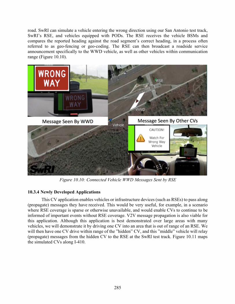
285

road. SwRI can simulate a vehicle entering the wrong direction using our San Antonio test track, SwRI’s RSE, and vehicles equipped with PODs. The RSE receives the vehicle BSMs and compares the reported heading against the road segment’s correct heading, in a process often referred to as geo-fencing or geo-coding. The RSE can then broadcast a roadside service announcement specifically to the WWD vehicle, as well as other vehicles within communication range (Figure 10.10).

Figure 10.10: Connected Vehicle WWD Messages Sent by RSE

10.3.4 Newly Developed Applications

This CV application enables vehicles or infrastructure devices (such as RSEs) to pass along (propagate) messages they have received. This would be very useful, for example, in a scenario where RSE coverage is sparse or otherwise unavailable, and would enable CVs to continue to be informed of important events without RSE coverage. V2V message propagation is also viable for this application. Although this application is best demonstrated over large areas with many vehicles, we will demonstrate it by driving one CV into an area that is out of range of an RSE. We will then have one CV drive within range of the ”hidden” CV, and this ”middle” vehicle will relay (propagate) messages from the hidden CV to the RSE at the SwRI test track. Figure 10.11 maps the simulated CVs along I-410.

286

Figure 10.11: Simulated CVs along I-410 in San Antonio Showing Potential for Message

Propagation between RSEs

Road Condition Monitoring (RCM)

According to current estimates, potholes cause approximately $6.4 billion in damage annually, making timely detection and repair of degraded roadways a significant concern for citizens and governments alike. Current methods for detection of poor road conditions consist of manual surveying, which is limited by the available resources of a traffic management entity. While the prevalence of smartphones has increased the ability for individuals to report road condition issues, the use of CV communication protocols presents a unique opportunity to enable vehicles to identify regions of pavement that require immediate maintenance, and to observe trends in pavement conditions over time. The necessary technologies to accomplish this, such as accelerometers, GPS-based localization systems, and CV DSRC are becoming more widely available, enabling new applications to be developed to enhance the collective situational awareness of the vehicles themselves, and of the traffic system as a whole.

10.3.5 Road Condition Monitoring

SwRI has developed a method for utilizing incoming accelerometer and GPS data to quantify road roughness, which can be scaled across various spatial windows that reflect different aspects of road health. For example, a smaller spatial window will detect shorter-term anomalies in road condition, such as might be caused by a pothole or piece of debris in the road, while a larger window will detect more general roughness on a segment of road, which may indicate road surface deterioration. Figure 10.12 shows RCM hardware evolution.

287

Figure 10.12: RCM Hardware Evolution

Because the response of an individual accelerometer will be affected by the specific dynamics of a vehicle, including tire and suspension response, the Dynamic Distributed Road Rating (DDRR) system is first trained using the accelerometer data from a specific vehicle installation. This training is performed by driving the vehicle through a variety of speeds on smooth roads to identify the system’s baseline response (as shown in Figure 10.14). Once completed, the vehicle is able to identify anomalous road pavement conditions, and communicate this data to other CV-equipped vehicles or to a RSE. This is reflected in the “vehicle” portion of Figure 10.13. Figure 10.14 provides a reading distribution from the system.

Figure 10.13: High-level Overview of the DDRR System.

Blocks represent processing steps and arrows represent transmitted data.

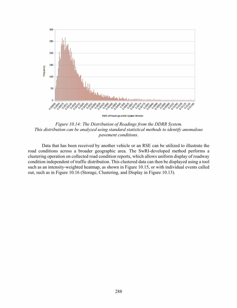
288

Figure 10.14: The Distribution of Readings from the DDRR System.

This distribution can be analyzed using standard statistical methods to identify anomalous pavement conditions.

Data that has been received by another vehicle or an RSE can be utilized to illustrate the

road conditions across a broader geographic area. The SwRI-developed method performs a clustering operation on collected road condition reports, which allows uniform display of roadway condition independent of traffic distribution. This clustered data can then be displayed using a tool such as an intensity-weighted heatmap, as shown in Figure 10.15, or with individual events called out, such as in Figure 10.16 (Storage, Clustering, and Display in Figure 10.13).

289

Figure 10.15: Heatmap Display of Road Condition in San Antonio, TX

Figure 10.16: Showing Precise Location of Anomalous Events

10.3.6 Dynamic Wrong-way Driving Detection

Vehicles that are equipped with the SwRI-developed portable onboard device (POD) system, which will be transmitting basic safety messages (BSMs) at 10 Hz, to drive the correct direction on our test track and through our four-way signalized intersection. The RSE located at the SwRI test track will be running a SwRI-developed machine-learning algorithm, essentially listening to the BSMs and learning the location of lanes and their correct direction of travel (Figure 10.17). Once this learning is accomplished, any connected vehicle traveling the wrong way, will be identified as a WWD, and the WWD warnings, as previously demonstrated, will be initiated.

SwRI’s R&D efforts on this program focused around the intelligent aggregation of basic vehicle state data such as GPS position, heading, and speed, passively collected by nearby infrastructure-based DSRC equipment using existing hardware solutions developed for CV

290

deployments. This aggregated data was then processed using SwRI-developed learning algorithms and condensed into a set of sparse GPS waypoints that represents the lane-level roadway model. This set of waypoints can then be broadcast out by the RSE and received by DSRC-equipped vehicles for use in numerous safety and mobility applications. The lane-level model can also be rebroadcast by vehicles to other vehicles that are not within range of the RSE, or could be broadcast and received using cellular communications, thus greatly expanding the number of vehicles that can benefit from the map data.

As vehicles repeatedly pass over lane segments, the stationary RSE collects the vehicles’ BSM data, which will vary slightly from vehicle to vehicle as individual drivers may pass over a given lane segment in different positions within the lane, and due to small variations in GPS accuracy. However, the more frequently vehicles pass over the same lane segment, the more data the learning algorithm has to analyze, and the faster it can converge on a steady-state model of the lane. This iterative process results in an increasingly accurate representation of the centerline of a lane segment, which can be updated dynamically simply through the altered behavior of drivers. The algorithms SwRI has developed can detect this altered behavior after a threshold of vehicles have traversed the same segment, and the lane model can be updated and rebroadcast quickly without centralized control of the process.

BSM data sets are evaluated as groups of line segments that correspond to “path history” points as defined in SAE J2735. SwRI began with an assumption that once a sufficient number of vehicles pass over a given lane segment that a normal distribution of GPS points within the lane width will begin to emerge. The learning algorithms begin by grouping line segments together and then calculate the perpendicular distance and angle of separation with all other line segments for a given segment of lane. After candidate groups have been identified, outlier segments are identified using Chauvenet’s criterion, and removed, and the mean absolute error calculated. It is desirable to minimize this error, which is then assumed to be the center of the lane for that location. This does not necessarily mean the absolute center of the physical lane has been identified, just that the center path driven by a number of vehicles has reached convergence based on this method. This method, however, is susceptible to halting on local minima, and so a minimum group size is required before the process is allowed to halt.

Histograms are then calculated for each group to determine if and where significant peaks exist. Selected potential lane segments must be within one lane width of a root segment. When all lane segment groups have been evaluated and the roadmap has been populated with high-likelihood lane-level.

291

Figure 10.17: Dynamic Lane Learning

292

10.4 Demonstrations

10.4.1 Winter 2017, J.J. Pickle Research Campus

In December 2015, the project team organized a demonstration of the applications described above at the J.J. Pickle Research Campus in Austin, TX. A quarter-mile stretch of road was closed off to normal traffic on the campus’s south side where the team conducted demonstrations to an audience of TxDOT staff, and UT Austin faculty and staff not associated with the project, as shown in Figure 10.18. These demonstrations enabled the attendees to ride in connected vehicles during the demonstrations to view first-hand how various CV applications might be implemented.

Figure 10.18: Winter Demonstration Venue Showing J.J. Pickle Research Campus (Inset), and

Detail Location of Test Road and Temporary RSE

Attendees who were not riding in vehicles could view the demonstrations from a safe viewing area, labeled “Base” in Figure 10.19, and could see various DSRC hardware as well as a large TV screen that showed the real-time locations of the vehicles on a Google Earth map overlay.

293

Figure 10.19: Winter Demonstration Venue Showing Effective RSE Coverage Area, Viewing

Area, and CV Vehicles During a Demonstration

10.4.2 Spring 2016, SwRI and San Antonio Roadways

In June 2016 the project team organized a second set of demonstrations, this time in San Antonio, TX. These demonstrations enabled the team to highlight the installed base of RSE devices in San Antonio, with one located on SwRI’s campus and three installed along Interstate 410 between Culebra Road and US-281, as shown in Figure 10.20. Specifically, the road condition monitoring, message propagation, and dynamic WWD detection and alert demonstrations were able to take advantage of these RSEs, and demonstrate the power of these CV applications in a larger geographic area than was possible during the winter demonstration.

SwRI was also able to showcase one of its fully autonomous vehicles, a Class VIII Freightliner, during the dynamic WWD demonstration. The Freightliner was sent along a route as a WWD, and once the local RSE detected this and warned the vehicle of its WWD status, the vehicle was autonomously brought to a controlled (safe) stop before it could enter the primary route for “right-way” drivers. This simulates an autonomy-capable vehicle approaching a highway the wrong direction on an exit ramp, either in an autonomous driving mode or under human control, and upon notification by the RSE, which sends out a trusted and verified message, the vehicle will slow and stop prior to entering the main lanes of the highway.

294

Figure 10.20: Spring Demonstration Venue Showing the Campus of SwRI and a Portion of

Interstate 410 Instrumented with RSEs

10.4.3 On SwRI’s Test Track: Dynamic WWD Detection and Alert with AV Safe Stop

SwRI will demonstrate a new method for implementing WWD Detection utilizing machine learning algorithms, and will show how an automated vehicle can be safely stopped before becoming a hazard to right-way drivers. To accomplish this, SwRI will first use two or three vehicles that are equipped with the SwRI-developed portable onboard device (POD) system, which will be transmitting BSMs at 10hz, to drive the correct direction on our test track and through our four-way signalized intersection. The RSE located at the SwRI test track will be running a SwRI-developed machine-learning algorithm, essentially listening to the BSMs and learning the location of lanes and their correct direction of travel. Once this learning is accomplished, any connected vehicle traveling the wrong way, will be identified as a WWD, and the WWD warnings, as previously demonstrated, will be initiated. In this instance, SwRI will utilize a fully autonomous Class VIII Freightliner as the WWD vehicle, and upon receiving the WWD alert from the RSE, the vehicle will come to a controlled (safe) stop, prior to entering the main lanes of right-way driver traffic.

295

Figure 10.21: Dynamic Lane Learning at SwRI’s Test Track

SwRI was also able to showcase one of its fully autonomous vehicles, a Class VIII Freightliner, during the dynamic WWD demonstration. The Freightliner was sent along a route as a WWD, and once the local RSE detected this and warned the vehicle of its WWD status, the vehicle was autonomously brought to a controlled (safe) stop before it could enter the primary route for “right-way” drivers.

Figure 10.22: SwRI’s Autonomous Freightliner Stops Once Identified as a WWD

Figure 10.23: SwRI Autonomous Freightliner

This simulates an autonomy-capable vehicle approaching a highway the wrong direction on an exit ramp, either in an autonomous driving mode or under human control, and upon notification by the RSE, which sends out a trusted and verified message, the vehicle will slow and stop prior to entering the main lanes of the highway. Additionally, at the SwRI test track, a large TV screen will display a Google Earth map showing semi-live updates on from mobile (off-campus) demonstrations, including Road Condition Monitoring and Message Propagation. This

296

display will give attendees a sense of the type of data that could be available to a DOT such as TxDOT, with even sparse deployment of CVs and RSEs.

10.4.4 On and Around Loop 410 in San Antonio

SwRI will utilize the installed base of RSEs in San Antonio to demonstrate road condition monitoring and message propagation. The Road Condition Monitoring demonstration will be conducted using a team of vehicles, which will take participants onto San Antonio streets and I-410. In the vehicle, an Android tablet will display the real-time data ”rough roads” and ”pot holes.” Roughness events that exceed a threshold will be cached onboard until the vehicle comes within range of an RSE, at which time the data will be sent to the RSE and forwarded on to SwRI computers at the test track and displayed as a heat map of locations and severity. This data could be shared with other vehicles to warn or advise of rough roads, and would be very valuable to TxDOT for real-time maintenance awareness.

Figure 10.24: Road Condition Monitoring Tablet and Heat Map Displays

Message Propagation - This CV application enables vehicles or RSEs to pass along (propagate) messages they have received. This would be very useful, for example, in a scenario where RSE coverage is sparse or otherwise unavailable, and would enable CVs to continue to be informed of important events without RSE coverage. This application is best demonstrated over large areas with many vehicles; however, we will demonstrate it by driving one CV into an area that is out of range of the SwRI RSE, and a second CV will be positioned within range of the first (hidden) CV. This second (bridge) vehicle will relay (propagate) messages from the hidden CV to the RSE at the SwRI test track, and its message will be displayed on the TV over a Google Earth map overlay, along with message propagation meta-data such as the number of hops taken, in this case just one, and the time it took to propagate from source to destination.

297

Figure 10.25: Message Propagation Demonstration Configuration

298

Chapter 11. Demonstration of Technology: CTR

This chapter summarizes this project’s demonstration of technology helmed by the Center for Transportation Research.

11.1 Introduction

Transportation research is currently at a tipping point: the emergence of new transformative technologies and systems, such as vehicle connectivity, automation, shared-mobility, and advanced sensing is rapidly changing the individual mobility and accessibility. This will fundamentally transform how transportation planning and operations should be conducted to enable smart and connected communities. The transportation systems can be substantially improved, and become safer, more efficient and reliable, thanks to the emergence of connected and autonomous vehicle technology. Dynamic routing and traffic-dependent navigation services are already available for users. Such applications need to estimate the present traffic situation and that of the near future at a forecasting horizon based on measurement data available in real-time, possibly supplemented with past data on traffic patterns. Using this measurement data and prior information, one can estimate the state of traffic on a road network, which consists in estimating all the traffic variables (e.g., cars density, speed), everywhere in the network, at the current time. This estimation requires the fusion of traffic data and traffic models, which are typically formulated as partial differential equations (PDEs).

In this report, we identify two possible improvements to the problem of traffic state estimation (that is, creating traffic maps and forecasts from traffic measurement data), that directly result from the presence of connected autonomous vehicles (CAVs). These improvements can be summarized as follows:

1) Using vehicle connectivity to generate traffic measurement data automatically, relying on the currently available traffic monitoring infrastructure. In the present case, our objective is to investigate the use of Inertial Measurement Units (IMUs), which can act as position sensors, while preserving user privacy. These IMUs can send traffic measurement data over Bluetooth, to currently available Bluetooth traffic readers.

2) Since these IMU sensors generate trajectory estimates, which typically differ from the measurement data generated by both GPS sensors and fixed traffic sensors, our objective is to design a computational scheme that can integrate the trajectory estimates generated by the IMU sensors into traffic flow model, to generate traffic maps.

11.2 Background

Most car navigation systems estimate the car position using satellite-based positioning systems, such as the Global Positioning System (GPS) (Figure 11.1). Other satellite-based systems are available, such as the GLONASS system, or the upcoming Galileo System, though such systems are not currently offering worldwide coverage.

299

Figure 11.1: Illustration of a Constellation of GPS Satellites Orbiting the Earth

GPS positioning systems operate as follows: a set of satellites transmit pulses at regular time intervals, which can be received by a GPS receiver. If four satellites signals are simultaneously received by the user, the user can determine its position and time by solving a system of four equations with four unknowns, where the equations correspond to the times required for the signals of the satellites to reach the GPS receiver, and the unknowns correspond to the position on Earth (longitude, latitude and altitude), as well as the current time.

GPS satellites operate on two communication channels (L1 and L2), operating at a very high frequency, on the order of 1GHz. The L1 channel carries the Navigation Message, which is transmitted at a very slow rate of 50 bits per second (bps, or Baud). It is a 1500-bit sequence, and therefore takes 30 seconds to transmit. This Navigation Message includes information on the Broadcast Ephemeris (satellite orbital parameters), satellite clock corrections, almanac data (a crude ephemeris for all satellites), Ionosphere information (which is used to correct the delays received by the receiver in function of the state of the Ionosphere, an atmospheric layer located between 60km and 1000km altitude), and satellite health status.

While GPS systems are relatively inexpensive and accurate (up to tens of meters in usual conditions), they have several drawbacks for traffic sensing applications:

1) The positioning information is affected by random noise, particularly in urban environments. This random noise is caused by the unwanted reflections of the satellite signals on buildings, which affect the accuracy at which one can precisely time when the signal of each satellite was received, and therefore causes positional errors (canyon effect). In urban environments, these errors can be on the order of tens of meters, which can cause for example a vehicle equipped with a GPS to appear to be driving on another street. This can result in a loss of precision for traffic purposes: while the mapping of the vehicle to the road network is usually correct, it may be that the fluctuations in the estimated position (from the GPS measurements) cause high uncertainty in travel time estimates between two consecutive intersections. Similarly, when monitoring traffic in urban environments, the GPS uncertainty prevents one from accurately distinguishing vehicles stopped in traffic, or parked vehicles (such as vehicles waiting for a passenger). Higher resolution GPS systems are available; for example, Real-Time Kinematics (RTK) GPSs use measurements of the phase of the GPS signals emitted by satellites to pinpoint the position of a receiver with greater accuracy. As of 2016, however, these devices cost hundreds of dollars, and require minutes to tens of minutes to properly lock on GPS satellites.

300

2) While the generation of absolute position data (longitude, latitude, and altitude) is desirable from a positioning standpoint, it inherently affects the privacy of the user when part of a traffic monitoring system. Indeed, classical traffic monitoring architectures (such as the architecture used in the Mobile Millennium experiment at UC Berkeley) for GPS-based traffic sensing rely on GPS position measurements sent by users to a given centralized server, as illustrated in Figure 11.2. As can be seen from this figure, the traffic data generated by vehicles (in the form of velocity and position measurements) is first sent to a third-party server (over the cellular network), which attempts to anonymize the data (for example by stripping the phone number associated with the GPS position information), and subsequently transmits this data to computer servers that perform the traffic state estimation (using possibly other traffic feeds, such as from fixed traffic sensors or other sources of traffic information). The major issue associated with this architecture is that the third party has access to all information about the user, and therefore has to be trusted.

Figure 11.2: Architecture of Classical Traffic Monitoring Systems (Probe-Vehicle Based).

In this system, traffic measurement data is sent to an anonymization server, which holds sensitive information.

Figure 11.3 outlines a different type of traffic monitoring architecture based on a short-

range wireless radio network. In this architecture, the data generated by vehicles is processed in a distributed manner by the fixed radio nodes themselves.

Figure 11.3: Architecture of a Distributed Probe-Based Traffic Flow Monitoring System, which

Guarantees User Privacy. Unlike current systems, the measurement data is not centralized, and local nodes only have

access to local measurements. The advantage of such a system is that privacy is guaranteed by design, since only a

distributed attack on the radio nodes would allow an adversary to gain information on the location of users.

Bluetooth or WiFi readers are widely used across the United States and the world to generate traffic measurements. They operate as follows. A vehicle carrying a Bluetooth or WiFi

301

enabled device (for example, a Bluetooth-enabled cellphone, or a WiFi-enabled tablet) drives between two different readers. Each reader captures the MAC (Medium Access Control) of the device by performing a scan. The MAC is unique to each device. Therefore, the operator of the sensing infrastructure can match the MAC addresses collected by the readers, and determine the travel time required to go between one reader to the other.

The main issue associated with Bluetooth or WiFi readers is their inherent tradeoffs. The devices cannot be installed too far apart from each other, as the probability of matching vehicles decreases when the distance between readers increases (since vehicles are less and less likely to take the route between the two readers). A notable exception is highways, since most users can only take one route between two readers. Similarly, Bluetooth or WiFi readers cannot be installed too closely from each other, as this would result in added uncertainty, due to the detection range of the Bluetooth or WiFi signals, in the order of tens of meters.

Thus, the proposed IMU system can interface directly with Bluetooth readers, providing an additional and complementary data feed to this system

11.3 IMU-based Traffic Flow Monitoring

11.3.1 Inertial Measurement Units

An Inertial Measurement Unit, or IMU, consists of the combination of an accelerometer, a gyrometer (or gyroscope), and possibly a magnetometer, in a single device. IMUs are commonly used in aerospace engineering to estimate the position of aircrafts or spacecrafts, by monitoring the accelerations and rotations of the vehicle in which the IMU is located. IMUs are also used in connected and autonomous vehicles to monitor their acceleration and attitude with respect to the ground.

The accelerometer of an IMU measures the proper acceleration, which is the acceleration of an object with respect to a free-falling frame. The proper acceleration (sometimes referred to as g-force) is different from the actual acceleration of the object (sometimes called coordinate accelerations). In this project, we are not interested in matching the accelerations to causes (external forces), since we only want to reconstruct vehicle trajectories

The gyrometer (or gyroscope) of an IMU measures the rate of rotation of an object with respect to an inertial frame. Newtonian mechanics postulate that all inertial frames are in uniform translation with respect to each other, and therefore have no rotation motion with respect to one another. Such frames are approximated by frames that use reference points that are very far away from us (for example stars or galaxies). The gyroscopes measure the rate of rotation of an object with respect to these frames, by measuring the Coriolis pseudoforce caused by the rotation on a test object.

The magnetometer is a device that monitors the direction and amplitude of the local magnetic field, and can therefore be used as a directional reference by tracking the direction of the magnetic North. Given that vehicles are built with high amounts of steel, which is ferromagnetic (and thus strongly perturbs magnetic field lines), the measurements of the magnetometer are in practice too unreliable to be used as a directional reference.

11.3.2 Fabrication of a Bluetooth IMU Device

To facilitate the integration of the IMU with a vehicle, we chose to build our own IMU system using hardware components, integrated in a printed circuit board (PCB). The objective was

302

initially to use the IEEE 802.15.4 RF protocol to transmit position data to a given wireless sensor network, and as a result, the system has a slot for an 802.15.4 XBee transceiver. An early prototype of the system is shown in Figure 11.4:

Figure 11.4: Top: Early IMU Prototype. Bottom: Second Iteration of the PCB Layout.

The early prototype shown in Figure 11.4 is built around an ARM Cortex M4 processor, handing an IMU connected to the processor using the I2C protocol, a type of digital communication protocol. A Bluetooth module (located under the system) is connected to the processor using serial communication, which is another form of digital communication. The USB port is used to supply regulated current to the system, and as a way to rigidly attach the IMU to the vehicle. The final version (shown in the bottom of Figure 11.4) is slightly larger to accommodate the GPS antenna and SD card slot. The final iteration of the IMU prototype is shown in Figure 11.5. This figure also shows the different peripherals connected to the main processor.

303

Figure 11.5: Bluetooth, IMU, and SD Card Peripherals of the Developed Sensor

To validate the performance of the sensor in trajectory reconstruction, we also included a GPS system (which is only used for validation). The GPS has its own antenna, and also communicates to the main processor using serial communication. It is shown in Figure 11.6.

Figure 11.6: GPS and JTAG Programming Interface of the Sensor

To program this sensor, we use a JTAG (Joint Test Action Group, which is an electronics industry association formed in 1985 for developing a method of verifying designs and testing printed circuit boards) interface. JTAG interfaces are commonly used for developing printed circuit boards, and have standard connectors for programming the device. The JTAG interface and JLink programmer used to upload the code to the memory of the microcontroller is shown in Figure 11.7:

304

Figure 11.7: JTAG Programming System. Left: RS232 Interface. Right: JLink Programmer.

11.3.3 Validation of the Different Components

The second set of activities consists of developing software to interface with the sensor, and communicate with its different subsystems (for example, Bluetooth, GPS, and IMU). This requires the development of software libraries. These libraries allow the microcontroller to establish a connection with its peripherals, retrieve the data they generate (for the GPS and IMU), configure their performance characteristics (for example, the rate at which they send measurement data or their scales), and outputs this data (such as by sending them to a Bluetooth-enabled device, or by storing them in a micro SD card).

Since embedded systems have an emphasis on performance and low cost (with respect to other consumer electronics), they tend to be unreliable, which requires an intensive debugging process.

The different components have subsequently been tested by installing the device in a vehicle, connecting it either to a free USB port, or to a USB car charger. An example of installation is shown in Figure 11.8.

Figure 11.8: IMU Device Installed in a Vehicle, with Power Supplied through a USB Car

Charger

305

The Bluetooth connectivity was subsequently tested by installing a Bluetooth terminal application (in the present case the BT Simple Terminal app developed for Android) on a smartphone (Samsung Galaxy Mega 2), and paired with the device. The default pairing code chosen (1234) is static for simplicity, although more sophisticated and secure pairing schemes could be created.

The inertial measurement data consists in a vector with six components: = ,

which corresponds to the vector of proper acceleration measured in the set of coordinates defined by the IMU sensor. = ,

which corresponds to the rotation vector, measured in the set of coordinates defined by the IMU sensor.

Note that the rate at which data is generated by the sensor is a function of the dynamics

that we want to track. For land vehicles, the spectrum of the accelerations and rotation rates contains frequencies that are relatively low, on the order of a few Hz. Therefore, we choose a sampling rate of 10Hz, which is sufficiently high to cover all significant frequency components of the signal (by Shannon’s sampling theorem). The sampling rate should also be as low as possible, since the random noise affecting the signal increases with higher sampling rates. Figure 11.9 illustrates the reception of data on a smartphone over Bluetooth.

Figure 11.9: Illustration of Inertial Data Reception on a Bluetooth-enabled Smartphone

306

11.3.4 Inertial Data Validation

We conducted some tests to validate the performance of the IMU component of the system, by performing a few checks:

• The norm of the acceleration vector = should be close to the value of (acceleration of gravity at the surface of the Earth)

• We align each of the three axes of the IMU in the direction of the vertical, to check that each of the axes has a correct acceleration measurement. The variability of the acceleration measurement between axes is caused by factory calibration and accelerometer bias

The norm of the acceleration vector is shown in Figure 11.10. As this figure illustrates, the

norm is very close to the acceleration of gravity g (about 980 / ), and within the 2% error specified in the IMU parameters. The x axis corresponds to the time sample, over an experiment time of 75 seconds (with 10 measurements per second).

Figure 11.10: Norm of the Acceleration Vector (Units: / )

As this figure demonstrates, the proper acceleration is always very close to 1000 / , which corresponds to the acceleration of gravity on Earth.

Figures 11.11 and 11.12 show examples of raw acceleration and rotation rate measurement data, obtained from the accelerometer and gyrometer.

0200400600800

1000120014001600

1 26 51 76 101

126

151

176

201

226

251

276

301

326

351

376

401

426

451

476

501

526

551

576

601

626

651

676

701

726

751

307

Figure 11.11: Acceleration (Unit: / ) along the Three Axes of the Accelerometer during a

Car Trip. Since the axes of the accelerometer were not perfectly aligned with the natural axes of the

vehicles (longitudinal, lateral and vertical), the signal is difficult to interpret.

Figure 11.12: Rotation Rate Measurement Data (Units: / )

11.3.5 GPS Free Auto Calibration of IMU Onboard Vehicles

In Figures 11.11 and 11.12, the IMU is not aligned with the coordinate axes of the vehicles, which are defined as follows:

• Longitudinal axis: x axis

• Lateral axis: y axis

• Vertical axis: z axis

-1500

-1000

-500

0

500

1000

1500

1 29 57 85 113

141

169

197

225

253

281

309

337

365

393

421

449

477

505

533

561

589

617

645

673

701

729

757

Series1

Series2

Series3

-40

-30

-20

-10

0

10

20

30

1 31 61 91 121

151

181

211

241

271

301

331

361

391

421

451

481

511

541

571

601

631

661

691

721

751

Series1

Series2

Series3

308

The axes of the IMU are not necessarily aligned with the aforementioned axes. The relationship between the coordinates of the acceleration and rotation rate vectors in the vehicle axes and in the IMU axes is encoded by a rotation matrix : =

where A correspond to the coordinates of the acceleration vector in the vehicle frame, and a correspond to the coordinates of the acceleration vector in the IMU frame. This misalignment is one of the main issues of retrofitting an IMU to a vehicle. Unlike a GPS, an IMU requires calibration, which makes the retrofit too complex. We thus investigated a way to perform this calibration automatically.

Procedure

Let ( ), ( ), and ( ) be the rotation matrices transforming respectively the vehicle

coordinates into the ground coordinates, the IMU sensor coordinates into the ground coordinates, and the IMU sensor coordinates into the vehicle coordinates. Our objective is to determine ,

which is assumed here to be constant ( is only representing the coordinate change between the

IMU and the vehicle, and unless the IMU is rotated with respect to the vehicle, this transformation remains constant). Since we do not have GPS or magnetometer data, (which corresponds to the

mapping between the IMU coordinates and the ground coordinates) cannot be determined univocally, though this does not affect the self-calibration principle.

Using the above definitions, we have that ( ) × ( ) = ( ) ( by the composition of

rotations). We assume that the pitch and roll attitude of the vehicle with respect to the ground is most of the time zero, given that most of the time, the vehicle lies flat on the surface of the Earth; that is, the vehicle does not have any roll angle (or tilt with respect to its longitudinal axis) or pitch angle (with respect to its lateral axis).

With this assumption, we have that ( ) is (on average) a rotation matrix of a pure yaw,

of the form: cos( ) −sin( ) 0sin( ) cos( ) 00 0 1

Determining ( ) (up to a rotation with respect to the z axis of the Earth frame) can be

done by fusing (combining) the accelerometer and gyrometer data, using a complementary filter or a Kalman filter. Note that since no heading measurement is assumed to be available, this rotation matrix will be known up to a rotation around the vertical direction (z axis of the Earth frame). While the IMU contains a magnetometer, which could be used to obtain the heading of the vehicle, the presence of metal in a car greatly affects the accuracy of the readings of this device, and we chose to ignore its measurement data for the present application. Therefore, the two above

309

equations do not allow us to determine the attitude of the device with respect to the vehicle ( ) uniquely. To determine uniquely, we can leverage the residuals of the acceleration

measurements. Indeed, the proper acceleration of the vehicle will be (in the frame of the vehicle, neglecting the Coriolis acceleration due to the rotation of the vehicle around its z axis77): === =

where , , , , , , and respectively denote the acceleration components in the vehicle coordinates, the acceleration components in the sensor coordinates, the velocity of the vehicle in the Earth frame, and the rotation rate of the vehicle along the z axis in the vehicle coordinates. Since the gyro measures the rate of rotation, we use the following approach: if the rate of rotation is approximately zero 78, the second term in the above equation is approximately zero, which gives us an additional measurement constraint, enabling us to compute the rotation matrix .

We validated the performance of this algorithm in reconstructing the correct value of

by computing the acceleration in the Earth Frame, for the device shown in Figure 11.8. The results are shown in Figure 11.13. As this figure demonstrates, the algorithm correctly converges to a state in which both and are zero, as expected.

Figure 11.13: Convergence of the Attitude Angle Estimates (attitude of the IMU device with

respect to the vehicle) Derived from the Rotation Matrix Rs/c

11.3.6 Trajectory Estimation Using Calibrated IMU Measurements

We performed a test involving a single IMU onboard a vehicle to evaluate the ability of the system to reconstruct the trajectory, from inertial measurements.

77 The Coriolis acceleration is on the order of . , where is the yaw rate of the vehicle and is the speed of the vehicle (in the Earth frame). For usual vehicles speeds and yaw rates, the effect of the Coriolis acceleration is negligible. 78 To check if the rotation rate is approximately zero, we are thresholding for the norm two of the rotation vector in the device frame. The rotation of the Earth is negligible with respect to the measurement uncertainty of the gyrometer, and thus we can assume that a fixed object on Earth is associated with a zero rotation vector.

310

11.4 Fast Computational Scheme for Integrating IMU Data into the LWR Traffic Flow Model

In traffic flow theory, different typologies of “slow” vehicles (or platoons) can be modeled as moving bottlenecks. These obstructions in traffic streams are usually associated with the presence of buses in urban traffic, and trucks or simply slower vehicles on highways. All these situations, indeed, are characterized by a partially blocked road (typically the right lane), causing a capacity reduction. The concept of moving bottleneck can be extended to fixed bottlenecks, which represent static (spatially) and time varying capacity restrictions caused for example by traffic lights and traffic incidents.

Some of the main challenges of modeling moving bottlenecks consist of identifying and modeling features regarding their speed (depending on the traffic conditions and on the maximum speed of the vehicle), their discharging flow (maximum rate at which vehicles overtake) and the entity of queue held back. Several studies have highlighted the importance of the effects of moving bottlenecks on traffic (Munoz and Daganzo 2002; Daganzo and Laval 2005) and have developed methodologies to include them into existing traffic models. Gazis and Herman developed in 1992 a model based on the conservation of flow, unconditional existence of the flow-density relation, and independence of capacity state from the bottleneck state. The first complete formulation based on the Lighthill–Whitham–Richards (LWR) model was proposed few years later by Newell (1993; 1998) where the moving bottleneck is assumed to behave as in a scaled-down version of the freeway’s fundamental diagram not influenced by the bottleneck speed. In recent years, more comprehensive formulations of the moving bottleneck problem have been proposed by Munoz and Daganzo (2002), Leclerq et al. (2004), and Daganzo and Laval (2005). Other studies have focused on numerical methods to solve the fixed and moving bottleneck problems within the LWR model (Lebacque et al. 1998; Giorgi et al. 2002; Leclercq 2007).

Motivated by the problem of traffic state estimation using IMUs, we derive an algorithm based on the Hamilton Jacobi representation of the LWR model to simultaneously compute the state of the system (density map) and the moving bottleneck trajectories. The method we propose is very fast, and improves computational times by almost two orders of magnitude with respect to current methods based on the Cell Transmission Model (CTM).

The idea behind forward simulation of traffic with unknown exogenous trajectories is to perform state estimation, as follows. The IMUs provide us with trajectory measurements, which are known. The initial and boundary conditions of the problem are however unknown. In this chapter, our objective is to compute the trajectories of given vehicles, assuming that the initial conditions of the problem are known, which is the converse problem. This converse problem can be used to solve the original problem, as part of a classical estimation framework, for example based on Particle Filtering or Ensemble Kalman Filtering:

1) Define candidate initial and boundary conditions, in some feasible set

2) Compute the trajectories of the moving bottlenecks representing the IMU equipped vehicles, using these initial and boundary conditions (propagation)

3) Use actual trajectory measurements from IMUs to select and filter the initial and boundary condition candidates (update), and use these updated candidates back in 1) The problem of computing the trajectories and parameters (passing flows) associated with

moving bottlenecks is not easy, since the bottlenecks both influence and are influenced by traffic.

311

Thus, in order to compute the density map associated with a general problem (involving initial, boundary conditions and bottlenecks), we have to simultaneously compute the solution to the LWR model and the corresponding trajectories of the bottlenecks, which is usually computationally intensive, since we have to map the solution on the complete computational domain. In the present report, we focus on moving bottleneck problems in which the passing flow is zero, that is, vehicles that are representative of traffic, tough the method introduced here could be extended to the case in which the passing flow is nonzero. We also assume that the IMU vehicles have the same performance as the rest of the traffic.

The algorithm we propose is based on an extension of the semi-analytical solutions to arbitrary Hamilton-Jacobi equations introduced in (Mazaré et al. 2011). Using semi-explicit solutions, we show that the trajectories of an arbitrary number of fixed and moving bottlenecks can be marched forward in time simultaneously for a very low computational cost. Indeed, if the piecewise affine initial conditions contain ni blocks, the piecewise affine upstream and downstream boundary conditions contain nu and nd blocks respectively, and i bottlenecks are considered, the future evolution of each bottleneck can be computed by at most (nu+nb+2) calculations of explicit functions, which determine the future value of the solution to the Hamilton-Jacobi equation along the trajectory of the bottleneck. Once this set of calculations is done, the future evolution of the moving bottleneck is completely determined, in function of the difference between the current value of the solution to the Hamilton Jacobi equation along the trajectory, and its future value along the predicted trajectory. This process is marched forward in time, and allows one to simultaneously compute the parameters associated with all moving and fixed bottlenecks of the problem, without having to compute the solution everywhere.

Once the parameters and trajectories of all moving and fixed bottlenecks are known, one can use this information to efficiently compute the solution of the problem everywhere using the Lax-Hopf algorithm (which was shown to be faster than the Godunov scheme if solutions are only required at the time horizon in Claudel and Bayen [2010a]).

11.5 Analytical Solutions to the Hamilton-Jacobi Partial Differential Equation (PDE)

11.5.1 The LWR PDE

Given a one-dimensional uniform section of highway, limited by x0 upstream and xn downstream. For a given time t and position x we define the local traffic density k(x,t) in vehicles per unit of length, and the instantaneous flow q(x,t) in vehicles per unit time. The conservation of vehicles on the highway is written as follows (Lighthill and Whithman 1956; Richards 1956; Garavello and Piccoli 2006): ( , ) + ( , ) = 0

For first-order traffic flow models, flow and density are related by the Fundamental

Diagram (FD); in this article we adopt triangular FD (Daganzo 1994). The FD is a positive function defined on [0,kj], where kj is the maximal density (jam density). It ranges in [0,qmax] where qmax is the maximum flow (capacity). It is assumed to be differentiable with derivative (0) => 0 (free-flow speed) and = < 0 (congested wave speed).

312

11.5.2 The Moskovitz Function

The Moskovitz function expresses the cumulated vehicle count N(x,t) and it represents the continuous vehicle count at location x and time t. In the Moskovitz framework one assumes that all vehicles are labeled by increasing integers as they pass the entry point of a highway section, and that they cannot pass each other. If the latest car that passed an observer standing at location x and time t is labeled n, then N(x,t)=n.

Replacing k and q with N yields to Hamilton-Jacobi PDE (Newell 1993; Daganzo 2005a 2006; Claudel and Bayen 2010a):

( , ) − − ( , ) = 0

11.5.3 The Generalized Lax-Hopf Formula

From Aubin et al. (2008), the solution associated with the value condition function c, denoted by , is the infimum of an infinite number of functions of the value condition: = { ( − , − ) + ( )} . . ( , ) ∈ , × ( − , − ) ∈ ( ) where c corresponds to: ( , ) = ( ) = 0( ) =( ) =

And ( ), which is the Legendre-Fenchel transform associated with the fundamental

diagram, is defined as: ( ) = sup, ( ( ) − ∙ )

This equation is well known in the Hamilton-Jacobi literature and often referred to as Lax-

Hopf formula (Aubin et al. 2008; Evans 1998).

11.5.4 Fast Algorithm for Triangular Fundamental Diagram

Assuming a triangular fundamental diagram, the calculation of its convex transform R yields to: ∀ ∈ , , ( ) = ( − )

Hence, the solution components associated with the initial and boundary conditions can be

expressed as follows. Initial conditions: If 0 ≤ ≤ , the initial condition imposes a free-flow state.

313

( , ) = − + ∶ + ≤ ≤ + − + + ( − ) ∶ + ≤ ≤ + else, if , ≤ ≤ : ( , ) = ( − ) − + ∶ + ≤ ≤ + ( − ) − + ( − ) + ∶ + ≤ ≤ +

For an upstream boundary condition defined as: ( ) = + with =− + ∑ ( − ) , the solution component can be expressed as:

( , ) = + − − ∶ + ( − ) ≤ ≤ + ( − )+ + − − ( − ) ∶ ≤ ≤ + ( − )

For a downstream boundary condition , defined as ( ) = + with =− + ( )( ) + ∑ ( − ) , the solution component can be expressed as: ( , ) = + − + ( − ) ∶ + ( − ) ≤ ≤ + ( − )+ + − + − ∶ + ( − ) ≤ ≤

11.5.5 Derivation of Internal Conditions for Multiple Bottlenecks

The algorithm used to compute the trajectory of the vehicle is leveraging the semi-analytic properties of the solutions of the Hamilton Jacobi equation, to enable one to compute the solution at a given point without having to march a grid forward in time.

1. Choose an arbitrary time step ∆ (Δ should be sufficiently large to have favorable

computational time characteristics, and sufficiently small to

2. Calculate the values of the Moskovitz function for: ( , ) = and ( +∆ , + ∆ ) = , where ( , ) corresponds to the position of the moving bottleneck in the end of the previous time interval, and corresponds to the maximum speed of the moving bottleneck.

3. If ≠ , do a line search on the domain {( + Δ , + Δ ), ∀ ∈ [0, ]} to identify such that ( + Δ ) = .

4. Update trajectory and go to 2.

In the above, = stands for the free-flow speed, is the critical density and is the number of lanes.

314

Once complete, the above process allows us to determine the solution to an arbitrary number of moving bottlenecks, which can be used to represent trajectory data generated by IMU equipped vehicles. We illustrate the performance of this algorithm by computing the density map associated with 11 distinct IMU trajectories in Figure 11.14.

Figure 11.14: Example of Simulation of Several Moving Bottlenecks.

The trajectory of each bottleneck is modeled by a yellow line, and the corresponding density is represented as a color map.

The algorithm that we developed consists in a new semi-analytic numerical scheme that

can be used to compute the solutions within the LWR traffic flow model given initial, upstream and downstream boundary conditions, and an arbitrary number of moving bottlenecks, which can be associated with different types of vehicles. The moving bottlenecks can be used to encode the trajectories of IMU equipped vehicles, for state estimation purposes.

This numerical scheme is based on a Hamilton-Jacobi formulation of the LWR model, and results from the properties of the solutions to Hamilton-Jacobi equations, and in particular the inf-morphism property. Being semi-analytic, it is very accurate (though not exact due to the piecewise linear approximation of the trajectories of the moving bottlenecks), and very fast, since it allows one to determine the trajectories of all moving bottlenecks without having to compute the solution on the entire computational domain, making it very adapted to traffic estimation problems resulting from the integration of large amounts of vehicle trajectory data (generated by GPSs or IMUs).

Through the use of IMU and computational algorithms, traffic states can be estimated from within a CV-system framework. One capability demonstrated here is successful operations without dependence on GPS data. Multiple, moving bottlenecks along a section of roadway can be tracked, which enables effective system-wide traffic optimization strategies.

315

Chapter 12. Economic Effects of CAVs

12.1 Introduction

Over the past decade or more, advances in the automotive and technology sectors have opened up the potential for the computerized-automation of the driving task. Every major automobile manufacturer and multiple technology companies, such as Apple and Google, have begun research and development of AVs. AVs may set off a revolution in transportation on a grand scale, across nations and continents. Any real transformation will require significant adoption or market penetration, but widespread use of AVs will generate a profound impact on many industries and markets throughout the U.S. economy and around the world.

To begin this discussion, it is useful to note that the USDOTW has defined five Levels of Automation (Aldana 2013). Level 0 implies no computer assistance for driving activities, while Level 1 involves function-specific automation for activities, like assistive parallel parking, adaptive cruise control (ACC), lane-keeping assistance (LKA), and electronic stability control (required on all new light-duty vehicles sold in the US since 2012). Level 2 is the combination of two or more of these features into a semi-autonomous vehicle—such as ACC plus LKA. Level 3 includes self-driving automation with full control of all critical safety functions under certain conditions—but the driver is still expected to take over in some instances (e.g., a confusing work zone or inclement weather). Level 3 will likely have significant economic impacts on the most directly related markets, such as the automotive and technology industries. Level 4 is the ultimate stage of automation, in which automobiles are fully self-driving without need for human intervention; they synchronize caravans of many vehicles and valet-park themselves. Connectivity between these vehicles will be developed in advance of and alongside rising automation, allowing for crash alerts, better coordination of vehicle speeds, and extended convoys. Once a large fleet of Level 4 connected AVs (CAVs) has been deployed, economic effects will increase and impact markets well beyond those directly related to AV production.

CAVs have the potential to generate widespread improvements in safety, time savings, and fuel savings, but their value extends well beyond these specific factors, into the broader economy. Although CAVs will naturally cause losses in some industries, the overall impact on the U.S. economy should be positive, as Morgan Stanley estimates an overall potential value of $1.3 trillion annually, or 8% of the entire U.S. GDP (Lewis 2014). An understanding of the trajectories of the specific business sectors affected, both positively and negatively, may be critical in effectively preparing for the economic impact.

Previous reports by companies like KPMG (2015), Morgan Stanley (2014), and McKinsey and Co. (2013), as well as research by Fagnant and Kockelman (2014), have examined different aspects of the U.S. transportation system and economy. This current chapter focuses on the economic effects of fully autonomous vehicles on specific markets by compiling and integrating economic research from top articles and studies. The markets evaluated are ordered beginning with the most directly and thoroughly impacted industries and end with more tangentially related markets. Analyzed industries include automotive, technology, freight movement, personal transport, auto repair, medical care, insurance, law, infrastructure, land development, digital media, police, and oil and gas. The chapter concludes with a look at the more wide-ranging effects on the economy such as improvements in safety, productivity, and fuel economy. Thoughtful examination of all these industries and CAVs’ more pervasive effects enables a valuable and rather comprehensive picture of likely impacts on the U.S. economy, which can significantly impact

316

policy, planning, investment, and design decisions, by public agencies, private businesses, investors, and the public at large.

12.2 Industries Analyzed

12.2.1 Automotive

The industry most obviously and directly affected by the design, adoption, and use of CAVs is the automotive industry. The auto industry is one of the driving forces of the U.S. economy, employing 1.7 million people, providing $500 billion in worker compensation annually, and accounting for about 3 to 3.5% of GDP (Hill et al. 2010). CAVs will influence not only the use and design of motorized vehicles but also redefine business strategies of companies within and outside the automotive industry. In a fully developed industry that is falling victim to stagnation and a decreasing interest among the young, AVs may revitalize many automotive companies (The Economist 2012).

One likely market expansion for vehicle production will come from increase in vehicle-miles traveled (VMT). This will be due to the ability of children, persons with disabilities, and elderly people to enjoy the convenience of automotive travel without the liability of physically driving the vehicle (The Economist). One report models four different scenarios for the effects of AVs on VMT based on increased capacity, changes in value of time, and reduced parking costs, and an alternative scenario in which all autos are automated and all costs are passed on to the user. The study found an increase in VMT ranging from 3.6% to 19.6% except for in the final scenario, where it estimates a decrease of 35.4% (Childress et al. 2014). The scenario in which all vehicles are autonomous will take decades to develop, if it ever does, so an increase in VMT is more likely in the short term. Private ownership of automobiles, however, may fall dramatically as “on-demand” car rental fleets and services develop, similar to Uber and Lyft, but driverless (Diamandis 2014, Fagnant and Kockelman 2015, Fagnant et al. 2015). Only 12% of all U.S. vehicles are in use/on the road during the nation’s peak moment (nearly 6 pm) of the average weekday, making vehicle sharing a very viable option (Silberg et al. 2013; Fagnant and Kockelman 2014). If vehicle sharing becomes a significant mode choice, it could decrease the personal demand for automobiles by millions of units every year, in the U.S. alone (Silberg et al. 2012). In 2015, automakers sold a total of 17.5 million cars and light trucks, totaling a cost of $570 billion for American consumers (Spector et al. 2016). Forbes Magazine (Diamandis 2014) estimated that this fact could cause the cost of transportation per mile to drop five- to ten-fold, though Chen et al. (2016) put the final monetary costs at closer to 50 cents per mile (versus the $0.57 to $0.74 per mile that AAA [2015] estimates for typical driving distances and vehicle types, as incurred by private-car owners in the U.S.). If SAVs gain a large share of the market but people continue to ride rather independently in these autonomous taxis, VMT may increase due to unoccupied/empty-vehicle travel between consecutive travelers and travelers’ preferences for more distant destinations (and perhaps more distant residential locations, over the longer term, leading to a more sprawling style of land development around many U.S. regions).

Alternatively, if carpooling and hub-and-spoke models for vehicle sharing become more widespread, VMT may decrease. According to a report by the University of Michigan Transportation Research Institute (Schoettle and Sivak 2015), if empty-vehicle driving of privately owned vehicles is allowed, CAVs may cause many families to choose to own just one car rather than two, if there is limited “trip-scheduling overlap” for different household members. In the most

317

extreme case, CAVs could cause a drop in personal ownership, from 2.1 cars per household to 1.2 cars per household, on average, representing a 43% reduction in the average number of household vehicles. However, heavier use of any vehicle will mean faster retirement or scrappage—though CAVs may crash much less often, resulting in somewhat longer lifespans—and lower car-buying rates (Li and Kockelman 2016, Fagnant and Kockelman 2014). Overall, total production and sales of passenger vehicles will probably rise, thanks to added demands for vehicle use, to more distant destinations. However, if shared vehicles are well maintained and so used for longer distances before retirement (much the way New York City taxis are used for far more miles than the typical household vehicle, before retirement), it is possible production rates will not rise as much as VMTs would suggest. New York City taxis travel approximately 70,000 miles per year, and the average age of a New York cab is 3.3 years (Bloomberg et al. 2014). Assuming a taxi life of 5-6 years, New York taxis travel around 350-400 thousand miles in their lifetime. A similar model of vehicle care could allow shared vehicles to experience similarly long lifetimes. Moreover, major fleet operators are likely to be sophisticated consumers and negotiators, and may want to purchase smaller vehicles, resulting in lower profit margins for vehicle manufacturers. Perhaps to insulate themselves from potentially big drops in demand or price, many OEMs are already teaming with transportation network companies, such as the partnerships of General Motors with Lyft, Toyota with Uber, and Volkswagen with Gett (Kokalitcheva 2016). With an estimated VMT increase of approximately 10% (Childress et al. 2014), a corresponding increase in vehicle sales would likely range from 5 to 10%, due to some of the growth being taken up by the rise of shared vehicles. Under this assumption, the number of cars sold per year would increase by 875,000 to 1.75 million, corresponding to an increase in sales by $28.5 to $57 billion. Although it is unclear how significant the factors affecting demand in each direction will be, automobile companies will undoubtedly face a very different landscape—in demand, suppliers, and pricing.

As demands shift, companies will want to strategically re-position themselves, in order to adapt to the industry’s fundamental evolution. Once fully autonomous vehicles become pervasive, greater emphasis will be placed on software and digital media (versus basic vehicle performance), forcing organizations to specialize in certain areas. Jonas et al.’s (2014) report for Morgan Stanley suggested that the auto industry may be completely reorganized into three key provider categories: hardware manufacturers, software suppliers, and integrated “experience” creators.

Hardware refers to the car essentially as we know it today (90% of the value of a current roadway vehicles (Jonas et al. 2014),and companies that choose to specialize in this segment will continue to design and manufacture the body, powertrain, interior, lighting, and other basic components. This position is likely for smaller car companies without a competitive advantage in software development, because they will not be able to invest enough resources to generate competitive/comparably intelligent in-car systems. These companies will outsource the software to businesses that specialize in automotive operating systems. As software’s importance increases, Jonas et al. (2014) argue that hardware will become increasingly commoditized, with only the most critical hardware components commanding significant pricing power, potentially dropping the relative value of hardware to 40% of the value of the car. In order to deal with falling margins on hardware sales, top vehicle manufacturers may add value through car sharing fleet operations, multi-modal journey planning, and other mobility-promoting services (Feick 2013).

Presently, car and truck software constitute approximately 10% of vehicle value. While influencing many automotive functions, the software-hardware interfaces are largely independent of each other. In CAVs, software components will become coordinated into a central, universal operating system, to control the powertrain, infotainment, and autonomous features, and may

318

eventually represent 40% of the car value (Jonas et al. 2014). Jonas et al. (2014) expect that larger auto manufacturers, larger suppliers, and leading technology companies (like Google, Apple, and Microsoft) will be responsible for such production. Similar to the smartphone industry, software-focused companies are forecast to sell and install their operating systems in vehicles manufactured by companies specializing in hardware, while car companies with large sums of resources will be able to invest in their own software development to generate a cohesive, integrated experience. Although this evolution may decrease profit margins in the hardware segment, the increasing value of software gives stronger automakers a new opportunity to generate revenue and opens up the market for tech companies.

12.2.2 Electronics and Software Technology

As alluded to above, technology firms may have the most to gain from the development of CAVs. Technology firms may emerge as entertainment providers and/or important players in the vehicle-production process, thanks to their competitive advantages in artificial intelligence (AI) application (Jonas et al. 2014 AI has become rather critical to making real-time/rapid human-like judgements in complex transport settings (e.g., navigating a new intersection with various bikes and pedestrians present, alongside a right-turning heavy-duty truck or bus).

Google’s self-driving cars have travelled over 1 million miles in California, with only 12 accidents - and none deemed the Google car’s responsibility (Google 2015). Much speculation has surrounded Apple’s entering the AV game, under possible name “Project Titan” (Price 2015). Intel Capital’s director confirmed that Intel recently launched a $100 million Connected Car Fund to “spur greater innovation, integration, and collaboration across the automotive technology ecosystem” (Silberg et al. 2012, p. 24). With all these big players investing significant time and capital into CAVs, it seems likely they will play an important role in the transport revolution and stand to gain large profits from it.

As noted earlier, Morgan Stanley estimates software costs rising from 10% of current car values to 40% in an AV environment (Jonas et al. 2014). IHS Technology’s Juliussen (2015) estimates that the U.S. self-driving software and its corresponding updates will grow from $680 million in 2025 to $15.8 billion in 2040. Similarly, IHS projects the built-in map and map-upgrade services to grow from $530 million in 2025 to $10.6 billion in 2040 (Juliussen 2015). Together, these services may offer $26.4 billion in new revenues over a 15-year period, for the U.S. alone. Software sales and the potential to integrate software into an entirely proprietary automobile, present major profit-making opportunities for technology firms. One challenge technology companies could face is the cyclical, price-sensitive nature of the automotive industry, which has not been so obvious in electronics and software markets (Jonas et al. 2014). Overall, revenues and profits from the second most expensive item most consumers purchase, after their home or rent, are very attractive, to a number of firms, especially those in the tech industry.

12.2.3 Trucking/Freight Movement

The economics of the trucking and shipping industry could also experience a significant boost from the development of AVs. Trucking companies could create convoy systems, allowing long distance drives with large quantities of goods and eliminating the need for a limit on the hours of service of the vehicles due to the limitations of the drivers. With intermodal transportation and logistics systems, the trucks could travel along major highways, transfer cargo at regional distribution centers, and then branch off for the final transfers directly to the packages’

319

destinations. This new system would improve safety and efficiency, saving trucking companies immense amounts of fuel, time, and money.

AV technology will likely be applied to commercial vehicles fleets early on, due to the large economic incentive for trucking companies. The next step of autonomy in commercial vehicles is assisted highway trucking, in which Level 1 or Level 2 AVs will help reduce truck collisions, through the use of features such as lane centering and adaptive cruise control. After assistive systems, fully autonomous vehicles will allow convoying, in which the lead driver of a chain of multiple trucks is in control of driving, but the following trucks require no human input and are connected wirelessly to the lead truck. Convoys do create issues with other traffic merging, changing lanes, and traffic signals, but this system could reduce accident rates and cut fuel consumption by 15% (Heutger et al. 2014). Even if drivers were required in the following vehicles, the time convoying could be counted as rest time, since the occupant/truck attendant could perform other activities, further extending the efficiency of the freight transportation system.

McKinsey estimates that the economic gains of driverless vehicles in the trucking industry could be range from $100-500 billion per year by 2025 (McKinsey 2013).

The bulk of these savings would come from the elimination of the wages of the truck drivers. According to the American Trucking Association (2015), the industry employs over 3 million truck drivers and the automation of driving poses a huge threat to the livelihood of these truck drivers. At this time, however, there is already a shortage of about 25,000 truck drivers because of the long hours and time away from home (American Trucking Association 2015). So, AVs could simply increase the capacity of logistics companies, allowing for more shipments. The role of the truck driver could become more technical, as they would need to monitor the AV system to ensure it is running properly. Such a role would likely require some training and could increase the value and wage of individual truck drivers. In such a scenario, the cost per truck driver would increase, but the number of hours of transportation per driver would increase and the number of drivers would decrease. AVs would undoubtedly be of massive benefit to the freight transportation and trucking industry but pose some risks for the employment of millions of truck drivers.

12.2.4 Personal Transport

AVs could also transform the transportation industry beyond the automotive industry, affecting trains, planes, and public transport. When vehicles no longer require an operator, occupants will be at liberty to use that time for productive work or even sleep. This found time on car trips might decrease the demand for fast transportation (Diamandis 2014). For example, if a destination is 10 hours away by car, a family or businessman may opt to make the trip overnight, sleeping while the car takes them to the destination, instead of making the flight. Bus, airline, train, and car rental companies could all be affected by the AVs’ added convenience. A possible development for bus companies to adapt to AVs is to develop a connected convoy system to transport a greater number of passengers on long trips. Platooning vehicles could also decrease the need for high-speed passenger rails. Fleets of platooning AVs could replace trains as a more fuel efficient and convenient solution to mass long-distance transit. Another possibility is that SAVs would provide easier access to these forms of mass transportation. Trains also have the added benefit of dedicated right-of-way, which avoids traffic congestion. With SAVs, passengers could be transported directly to the location of the bus, train, or plane without the need for parking their personal cars long-term. If VMT increases with the rise of AVs, such a system could allow travelers to avoid the higher cost of riding the full distance in their personal vehicle.

320

The biggest change in personal transportation as a result of development of AVs will likely be in short commutes. With AV technology, companies could develop an “on-demand” taxi service with SAVs that would make human-driven taxis obsolete. In fact, GM already has an autonomous taxi prototype that is summoned by a phone app. According to Frost & Sullivan (2013), Google is leading the way in a car-sharing business model and could be responsible for decreased car ownership. At peak vehicle usage during rush hour, around 5 PM, less than 12% of all personal vehicles are on the road (Silberg et al. 2013). The Brookings Institution makes an even bolder claim that vehicles sit unused an average of 95% of the time (Brookings 2014). Although the jobs of taxi and bus drivers will be threatened by AVs, “outsourced” driving accounts for less than 2% of personal transportation, so the impact to the wider economy will not be particularly large (TRB 2016). Vehicle sharing also has the potential to decrease these inefficiencies in our current transportation models.

While the effect on long-distance transportation is less clear, public transportation and taxi services are most directly affected by autonomous vehicles and shared fleets. The public transportation and taxi industries account for $66 billion and $20 billion in revenue, respectively (IBISWorld 2015, IBISWorld 2016). Ridesharing apps have already caused a 6.7% annual decrease in taxi service between 2011 and 2016 (IBISWorld 2016) and decreases as large as 30% in Los Angeles and 65% in San Francisco (Nelson 2016, Kerr 2014). With the addition of AVs to ridesharing services, a 50-percent decrease in taxi revenues would cause a shift in $10 billion in revenue toward ridesharing. Ridesharing and AVs are not as direct of a substitute for public transportation, and public transportation is less expensive compared to private driving services like taxis, so the shift would likely not be as pronounced. A 25% shift in public transportation revenues, however, still represents $16.5 billion in decreased public transportation revenue. In total, the changes in taxi and public transportation revenues account for $26.5 billion out of the total $86 billion in revenue, equating to a percent change of 30.81%. At the very least, AVs will take a bite out of the personal transportation providers like taxis, buses, and trains, and could extend as far as redefining car usage, making vehicle ownership more of a luxury than a necessity.

12.2.5 Auto Repair

With 360 degree sensors, no distractions, no drunk driving, among other characteristics, driverless cars will be able to largely eliminate car crashes caused by human error, which amount to over 90% of crashes in the U.S. currently (McKinsey 2013). Collision repair shops will lose a huge portion of their business. Indirectly, the decreased need for new parts for crashed vehicles would also decrease the demand for manufactured parts from steel producers and part manufacturers. In 2013, almost $30 billion in repairs were caused by vehicle crashes in the United States (Stahl 2014). Higher levels of market penetration will cause proportionally higher percent reductions in crashes. Assuming 25% reduction in crashes, the industry would lose $7.5 billion, and at a 50% reduction, auto repair dollars would decrease by $15 billion. Finally, at 100% market penetration, in the best case scenario, we would experience a 90% reduction in crashes and a $27 billion loss to the industry.

Some auto shops could find new opportunities in aftermarket personalization of vehicles, customizing the new, more important interior of the AV, but this will likely not be enough to cover the losses from their usual business (McKinsey 2013). As the level of autonomy increases and crashes fall, a large percentage of collision repair shops will lose revenues and be forced out of business. Despite the societal gain due to decreased crashes, collision repair shops are likely to face serious losses.

321

One effect that could be of benefit to the auto repair industry is the increased road time of AVs through sharing systems. Although there may be fewer total cars, the cars in use could be on the road for 12 hours per day, which will cause an increase in the miles travelled and the overall need for maintenance. AVs will still provide an increase in safety, but this increased number of road hours allows for more opportunities for crashes that would give business to the collision repair shops. The size of the impact on the industry is unclear, but collision repair businesses that retain their current model will likely face losses.

12.2.6 Medical

Another industry that will lose business from the improved safety of AVs is the medical industry. Approximately two million hospital visits and 240,000 extended hospitalizations per year in America are due to traffic accidents, and driverless cars would eliminate a large majority of these emergency room visits (The Economist 2012). McKinsey & Co. (2013) estimated that the combination of auto repair and health care bills could save consumers $180 billion, which would generate proportional losses for service providers. The National Highway Traffic Safety Administration estimates that motor vehicle crashes accounted for $23 billion in medical expenses (NHTSA 2015). With a 25% crash reduction, this accounts for a loss of $5.75 billion in the medical industry, $11.5 billion at a 50% reduction, and $20.7 billion at a 90% reduction. Although there will also be savings from the decreased need for supplies and doctors, and space could be cleared in overcrowded emergency rooms, the financial situation will be significantly altered for medical providers. Also, a large proportion of organ donations come from automobile crash victims who are registered organ donors, since they are younger and healthier at the end of their lives. Hospitals and emergency rooms profit from car accidents and could lose a large percentage of their business and supply with the elimination of human error in driving. A potential benefit for hospitals, however, is that they could reallocate personnel to better serve other needs. With emergency rooms often overrun with patients, this would allow hospitals to better serve patients.

12.2.7 Insurance

Safety improvements as a result of AVs will require insurance agencies to adapt and possibly reconstruct their fundamental business models. Currently, insurance companies sell policies to individual vehicle owners and human drivers are liable for car crashes. Insurance agencies currently net $180 billion annually in the U.S. insuring against automobile accidents and the related medical costs (Desouza et al. 2015). When driving becomes the job of computers, however, the issue of whether the driver is liable for the crash becomes much more ambiguous. Automakers and the vehicle’s software providers will likely become the main responsible party and will need to purchase insurance for technical failure of the automobiles, making personal policies more limited in scope (Silberg et al. 2012). Liability may be placed on the driver for authorizing driving in wet, icy, or otherwise unsafe conditions, causing a need for some coverage. However, greater responsibility, under normal circumstances, will likely shift to the software and hardware manufacturers.

Additionally, the added safety of CAVs that are nearly error-free will reduce the number of crashes significantly. According to a report by KPMG, over 90% of accidents each year are caused by driver error, and accident frequency could drop as much as 80% with commercially viable Level 4 fully autonomous vehicles (Albright et al. 2015). Even the automation of parts of the driving task has decreased insurance claim frequency. David Zuby, executive vice president

322

and chief research officer of the IIHS, claims that “vehicles equipped with front crash prevention technology have a 7-15% lower claim frequency under property damage liability coverage than comparable vehicles without it” (Albright et al. 2015). KPMG also hypothesizes that costlier technology under the hood of AVs could increase the average accident expense from today’s $14k to around $35k by 2040 (Albright et al. 2015).

Ultimately, KPMG estimates that AVs could shrink the auto insurance industry by as much as 60% (Albright et al. 2015). With the current revenue of the auto insurance industry at approximately $220 billion, this decrease could represent a loss of $132 billion. Insurers will need to develop fewer but larger corporate policies to maintain their businesses. Vehicle owners will still need insurance for theft and comprehensive coverage for hail, flooding, as well as more limited liability coverage which will likely cause a decrease in premium per policy (Insurance Business 2015). Overall, this could make small auto insurance companies based in personal policies less viable and give more power to large businesses based in corporate contracts. Since there are far more insurance companies than auto manufacturers, this push for large policies for autonomous systems will cause competitive insurance pricing and big winners and losers in the battle for these corporate contracts.

12.2.8 Legal Profession

The result of fewer accidents from the automation of driving will likely challenge the profession of many attorneys. Around 76,000 attorneys in the United States specialize in personal injury (Langham 2015). With a total number of around 1.3 million practicing attorneys in the United States, personal injury lawyers make up approximately 6% of the American lawyer population. Vehicle collisions are the most common type of tort case, accounting for around 35% of all civil trials (McCarthy 2008). Law school is already becoming a more challenging path because of a current oversupply of attorneys, and the decrease in demand for personal injury lawyers would hurt career prospects even further. With an average liability claim for bodily injury of $15,443, a total number of crashes of around 5.5 million in 2012, and an average contingency fee of around 33-40%, the economic implications of this development are immense, with potential losses as much as $3.2 billion for personal claim lawsuits (Langham 2015). The detriment to the profession could be offset by population growth and an increase in tort claims. Regardless, the landscape of the legal profession will be much different, at least in the scope of personal claims.

12.2.9 Construction and Infrastructure

Another AV impact is an altered need for infrastructure and construction of parking lots and new roadways. A potential increase in traffic efficiency would decrease congestion and the need for new, bigger roadways. If vehicle sharing reaches a sufficient level of development, a decreased need for parking would result and, thereby, reduce the demand for new parking lots and garages. Despite these increases in efficiency, it will likely be somewhat offset by the increase in VMT due to greater vehicle access and population growth. The designers and contractors of these large structures will ultimately get less business than they are used to and might need to adapt their businesses to include other types of infrastructure as a result.

Additionally, the way in which roadways are maintained and the component structures required may change. When vehicles become fully autonomous, there may no longer be a need for extra-wide lanes, guardrails, traffic control signals, wide shoulder, or rumble strips among other safety measures because of increased safety, and manufacturers of these components will lose a

323

source of income. With sufficient market penetration, C/AVs may be safe enough to allow the government to stop investing in these costly infrastructure safety measures. Data can be used by Departments of Transportation to analyze road use patterns and better plan the maintenance and improvements that are still needed. KPMG estimates that intelligently controlled intersections could perform 200-300 times better than current traffic signals (Silberg et al. 2012). KPMG also states that platooning could increase the effective capacity of roadways by as much as 500%, with a “conservative” estimate of a 10% reduction in infrastructure investment, saving around $7.5 billion per year (Silberg et al. 2012).

The infrastructure that is needed could be revolutionized alongside automobiles. An integral part of creating C/AVs is Vehicle-to-Infrastructure (V2I) communication. GPS, sensors, 3D planning, design, and construction tools can be used to help plan, design, and build more integrated and efficient transportation systems. With wireless transponders called Roadside Units or other smart embedded sensors, cars and roads can exchange information about curvy roads and low bridges, risks such as construction and information about traffic density, flow, volume, and speed (Bennett 2013). In order to remain competitive, contractors that base their business on large government commissions for highway and infrastructure construction will need to be on the cutting edge of this technology.

12.2.10 Land Development

AVs will change transportation for people in all parts of the nation, and, therefore, will impact our habits and land use. AVs will likely transform the national parking system. According to Eran Ben-Joseph, parking lots and garages cover more than one-third of the land area in some U.S. cities, creating unsustainable urban dead zones in centers where population density is increasing rapidly (Diamandis 2014). AVs will help mitigate this issue of overcrowding by allowing people to be dropped off at their location without the need to find a parking spot. On top of this, vehicle sharing will keep vehicles in more constant use and serve more people, further decreasing demand for parking infrastructure. According to a study by McKinsey & Co., the property savings from freed up land from parking as a result of the development of AVs could add up to $190 billion in the U.S. alone (Woodyard 2015). The land area previously used for parking could be converted into housing, parks, or other useful developments that replace these parking dead zones. Parking will become more efficient and demand will decrease with the advent of AVs, opening up land for other uses. The commercial real estate industry generates $931 billion in annual revenue, so the $190 billion in land could provide opportunity for a 20% increase in land development revenue (IBISWorld 2016).

Another possible impact of AVs on land development is the extension or contraction of urban sprawl. The automobile is the invention that originally caused the development of suburban neighborhoods due to the increased distance one could travel in a given period of time and the fact that land further from city center costs less per square meter. AVs could allow for a decrease in time of commutes and an increase in productivity during the commute as the passenger is no longer required to focus all attention on driving, which could increase the draw of suburban housing. With the ability to engage in activities other than driving during the commute, the cost of transportation declines, increasing the value of living further from the urban core (Anderson et al. 2014). Alternatively, AVs could cause a loosening in the urban real estate market, reducing the cost of urban living and encouraging families to move into town (Greeting 2014). Even with a freeing of urban space and potentially decreasing land prices, there is a limit to the total area of land in a city center and population continues to expand, which should cause the scenario of city expansion to

324

dominate as. There is a lack of research, at this point, on the effect of AVs on land use, which causes uncertainty in the direction of movement of urban and suburban development. However, it is important to pay attention to the impact on land availability and preference going forward for the development of real estate.

12.2.11 Digital Media

The extension of digital media into the AV environment will open up the market for even more users and, thereby, more sales. At the point of full autonomy, commuters that usually spend time vigilantly watching the road (or dangerously multitasking on their smartphones) will demand greater integration of digital media features into their automobiles. Content providers like YouTube, Netflix, and social media networks will see a large benefit from the increased time and desire for their services on commutes.

Additionally, a study by McKinsey & Co. suggests that internet shopping could receive a large bump from this added free time, stating that each additional minute occupants spend on the internet could generate $5.6 billion annually, totaling $140 billion if half of the time of the average round-trip commute (25 minutes) is spent surfing or shopping (McKinsey 2015). A possible loss due to this increase in entertainment flexibility for drivers is a decreased demand for radio and recorded music. Drivers will no longer be captive to audio-only entertainment, allowing them to forgo their usual radio programs for more stimulating visual ones. The boon for the overall entertainment market, however, could be quite significant, as a report from Morgan Stanley suggests the percent value of content in the automotive industry could shift from minimal to almost 20% of the value of the car (over $6,000 for the average cost of a car) (Jonas et al. 2014).

12.2.12 Police (Traffic Violations)

Due to human error and misbehavior in driving decreasing significantly, the importance of traffic cops and parking wardens will likely decrease as well. Drunk driving, speeding, and other traffic violations will become less frequent and the size of the police force will decrease (The Economist 2012). A survey by the Bureau of Justice Statistics shows that 31 million people were involuntarily stopped in 2011, more than 85% of those stops traffic related, and over half of all contact between civilians and police is related to vehicles (Zagorsky 2015). Another side effect of increased traffic obedience will be a loss of revenue for governments, as traffic fines make up a significant source of money.

According to the National Motorists Association (Bax 2008), the traffic ticket industry brings in between $7.5 to $15 billion. According to The Arizona Republic, approximately $10.8 million, or 1.1%, of Phoenix’s $1.03 billion budget in 2014 came from traffic ticket fines (Giblin 2015). Although $10 million is significant, a simple 1% of the city’s budget is recoverable from other sources. Small towns, however, may be more strongly affected by law-abiding AVs. While only five towns in Colorado earned more than 30% of revenue from traffic fines, the small city of Campo generated 93% of its budget from fines and forfeitures in 2013 (Kuntz 2015). These results are outliers from “speed trap” towns, but still this shift would be significant to these specific municipalities. Assuming a 50% reduction in the $10 billion in traffic ticket fines per year, AVs would account for a $5 billion decrease in government revenue. Some of this loss may be recovered, however, through savings from the decreased need for traffic police.

Government officials in small cities will have to find a way to adapt to this revenue loss. A decreased payroll due to fewer highway patrol officers will slightly offset this, but governments

325

could also make up for lost revenue by charging infrastructure usage fees (Silberg et al. 2012). One way to enable this solution with an established system is create more toll roads or even separate toll roads, similar to HOV lanes, for AVs that will be of value due to decreased traffic. Traffic tickets will not be eliminated until there is 100% market penetration of AVs, but the decrease in revenue will be felt gradually and local and state agencies will want to prepare for this change.

12.2.13 Oil and Gas

A more efficient system of driving will also cause ripple effects in the oil and gas industry. Platooning, computer-controlled, and lighter cars interacting with more efficient infrastructure will contribute to an overall improvement in fuel efficiency (Silberg 2012). The Texas Transportation Institute estimated that congestion costs Americans 4.8 billion hours of time, 1.9 billion gallons of fuel, totaling $101 billion in combined delay and fuel costs (Silberg 2012). Platooning could reduce highway fuel use by up to 20% solely due to the decreased drag coefficient from drafting (Silberg 2013). The decreased need for parking will improve fuel efficiency as well, as one MIT study found that 40% of total gasoline use in cars in urban areas is spent looking for parking (Diamandis 2014). Furthermore, SAV fleets could make electric vehicles a more viable option and even financially preferable for fleet management companies. All of these factors suggest that drivers would demand less gas for their cars. However, the improvement in fuel efficiency could also be joined by an increase in vehicle miles traveled (VMT) due to the newfound convenience and expanding housing limits.

12.3 Economy-Wide Effects

AVs will increase the capacity of the nation’s transportation system due to improvements in efficiency. First, with well-developed, accurate computing systems, traffic accidents, which account for 25% of traffic congestion, will be greatly reduced as approximately 93% of accidents are due to human error (Fagnant and Kockelman 2013). This fact will not only increase roadway capacity but also potentially save around $563 billion due to a reduction in injuries and deaths due to collisions (Jonas et al. 2014). Additionally, congestion will be reduced by the increased efficiency of coordinated vehicle speeds and traffic flow, due to data sharing between cars and synchronization of traffic signals, enabling a further increase in effective roadway capacity. The Center for Urban Transportation Research estimates that the connection of AVs will cause a 22% increase in highway capacity at 50% market penetration, 50% capacity increase at 80% market penetration, and 80% increase at 100% market capacity (Pinjari, et al. 2013). The increase in roadway capacity will likely be limited by a number of factors, as there is a finite limit to roadway capacity even in ideal conditions. VMT could increase, thereby increasing demand and decreasing the effective roadway capacity, both due to population growth and increase in accessibility. Population growth increases the raw number of potential drivers/riders. If AVs allow elderly and children to travel independently, an additional increase in VMT would occur due to increased access to previously unserved individuals.

Once the vehicles reach Phase 4 of autonomy with widespread adoption, they will enable children, elderly, and disabled people access to transportation. This will increase the number of vehicle miles traveled (VMT) and, thereby, slightly limit the decrease in congestion, but the increased efficiency should outweigh these effects (Pinjari et al. 2013). More importantly, this will allow a greater percentage of the population greater mobility which could improve productivity

326

nationwide. Productivity will also be increased as a result of the added time that can be used for other tasks, like working on the trip to the office. According to Forbes Magazine, AVs could save over 2.7 billion unproductive hours in work commutes, generating an annual savings of $447.1 billion per year in the U.S. alone (assuming 90% AV penetration) (Diamandis 2014). Fuel savings could amount to $158 billion, thanks to a 20-30% increase in fuel economy due to smooth driving and cruise control (Jonas et al. 2014). This savings estimate, combined with $488 billion from accident costs, $507 billion from productivity gain, $11 billion from fuel loss from congestion, amount to total savings of $1.2 trillion in the U.S., or 8% of the U.S. GDP, and as much as $5.6 trillion worldwide (Jonas et al. 2014).

Some effects brought on by AVs could counteract and limit these gains. Once AV sharing is put into action, although fewer cars will be needed, those in use will accrue mileage more quickly and require maintenance more often. Additionally, the increased convenience and affordability may encourage more vehicle travel, offsetting the pollution and crash benefits (Litman 2015). The economic effects of AVs will extend beyond the simple crash, productivity, and fuel saving into every facet of the American economy.

12.4 Conclusions

The purpose of this study was to identify the industries most impacted by the rise of CAVs and to examine the forces that affect these industries and the economy as a whole. Table 12.1 shows the 13 industries that were selected and ordered based on the immediacy and size of the impacts on each. The analysis showed a percentage change and overall dollar value change based on the size of the industry. Although individual businesses that do not adapt to this change may be hurt by the rise of CAVs, the economic effects were generally viewed as societal savings that would feed back into the economy through businesses and to consumers. On top of the effects on specific industries, everyone will experience the benefits of the time savings from decreased congestion and added productivity from the hands-free driving environment of CAVs.

According to the 2015 Consumer Expenditure Report, transportation accounts for 17% of average household income, 7.5% vehicle purchases, 3.7% on fuel, 1.2% on public transportation, and 4.9% on other vehicle expenses, such as maintenance and repairs and insurance (Bureau of Labor Statistics 2015). Comparatively, average household expenditures also include 32.9% for housing, 12.5% on food, 11.3% on insurance, 7.8% on healthcare, 5.1% on entertainment, 6.9% for utilities (Bureau of Labor Statistics 2015). Transportation will be directly impacted by the rise of CAVs, and nearly all of the other largest contributors to household expenditures will be heavily influenced by CAVs, as well.

CAVs will transform our economy and change the landscape of almost every industry. Although some sectors will be more significantly affected than others, ripple effects will be felt throughout most, if not all industries. The technology still has a long road of development ahead and market penetration will define the size of the impact of driverless vehicles. With the assumption that AVs will eventually become pervasive, or at least hold a large share of the automotive market, it is assured that they will have a strong economic impact, potentially as much as $1.3 trillion or more. In order to prepare for this revolution, we must be aware of the potential effects so that we can alter our established systems to accommodate these changes. Change is coming, and we must be prepared to adapt.

327

Table 12.1: Summary of Annual Economic Effects (Industry and Economy-Wide)

Industry-Specific Effects

Industry Size of Industry ($ billions per

year)

Dollar Change in Industry

($ billions per year)

Percent Change in Industry

$ Change per American per Year

by Industry

Automotive $570 $42 7.37% $131.61

Electronics & Software

$203 $26 13.04% $82.76

Freight Transportation

$604 $100 16.56% $313.48

Personal Transportation

$86 $27 30.81% $83.07

Auto Repair $58 $21 36.21% $65.83

Medical $2,700 $12 0.43% $36.05

Insurance $220 $132 60.00% $413.79

Law $277 $3 1.16% $10.03

Construction/Infrastructure

$169 $8 4.44% $23.51

Land Development

$931 $190 20.41% $595.61

Digital Media $42 $14 33.33% $43.89

Traffic Police $10 $5 50.00% $15.67

Oil and Gas $284 $101 35.56% $316.61

Industry-Specific Total

$6,153 $680 11.05% $2,131.97

Economy-Wide Effects

Collisions N/A $488 N/A $1,529.78

Productivity N/A $645 N/A $2,021.94

Fuel N/A $11 N/A $34.48

Economy-Wide Total

N/A $1,144 N/A $3,586.21

Overall Total N/A $1,566 N/A $4,907.84

328

Chapter 13. Concept of Operations (ConOps)

13.1 Overview and Scope of the Project

13.1.1 Background

The United States Department of Transportation (USDOT) has committed to the development of a fully connected transportation system that will enable advanced vehicle safety applications. The program began in 2006 as the Vehicle Infrastructure Integration (VII) program and is currently known as the Connected Vehicle (CV) program. This program has focused on a number of vehicle-to-vehicle (V2V) and vehicle-to-infrastructure (V2I) applications, such as forward collision warning (FCW), emergency electronic brake lights (EEBL), intersection violation warning, signal phase and timing (SPAT), signal prioritization and pre-emption, blind spot detection/warning, and others.

Increasing connectivity among vehicles, roadside devices, and traffic management systems creates the potential for both novel benefits to society as well as novel risks, particularly from the emerging cyber security risk to vehicles that are increasingly computerized and connected. The vulnerability of individual vehicles for targeted disruption has increased as their control systems, and even their entertainment systems, have shifted towards computer control, and greater connectivity. The evolution of Advanced Driver Assistance Systems (ADAS) towards semi- or fully automated vehicles also exacerbates this risk as the software may naively react to an Over-the-Air (OTA) message that is incorrect, whether benign or malicious.

13.1.2 Purpose of the Concept of Operations

A ConOps describes the goals and objectives of a system, and identifies user needs and high-level design criteria. Goals and objectives of the ConOps outlined in the document are intended to be high-level and may not necessarily be quantifiable or testable. Specifically, the ConOps document:

• Lays a foundation for the design, test, deployment, and implementation of smart transport technologies, such as CAVs.

• Provides a resource for the development of engineering requirements and supports decision makers in their assessments, deployment, and evaluations of the smart transport systems under a variety of scenarios and settings.

13.1.3 Intended Audience

A ConOps helps stakeholders focus on the proposed system’s capabilities and understand the effects on other internal and external systems and practices. Stakeholders of this ConOps document include TxDOT, researchers, local and state governments, law enforcement, private-sector agencies, system engineers and architects, system implementers, equipment manufacturers, and application developers. The ConOps also helps system engineers and architects to understand the constraints, assumptions, requirements, and priorities set forth to design and deploy smart transport systems.

329

13.1.4 Content and Organization of this Document

The ConOps is an early and critical step in the systems engineering process, and the purpose is to provide a description of why a system is needed and how it would be used considering the viewpoints of the various stakeholders. The ConOps:

• Describes the environment and use of the system in a non-technical and easy-to-understand manner.

• Presents the information from multiple viewpoints.

• Bridges the gap between the problem and stakeholders’ needs. Overall, the ConOps describes the basic who, what, why, where, when, and how a smart

transport is designed and deployed.

• Who – the stakeholders are, what their responsibilities are, how they will use the system.

• What – the existing components or systems to be examine and /or integrated together.

• Why – the problems or issues the system will solve.

• Where – the geographic limits of the system.

• How – the resources needed to plan, design, deploy, and operate the system.

13.1.5 Referenced Documents

While preparing the ConOps, the following documents were referenced:

• Guide for the Preparation of Operational Concept Documents, ANSI/AIAA/G-043-1992, American Institute of Aeronautics and Astronauts, Washington, D.C., 1993.

• Systems Engineering for Intelligent Transportation Systems: An Introduction to Transportation Professionals, USDOT, Washington D.C., 2007.

• IEEE 802.11p http://standards.ieee.org/getieee802/download/802.11-2012.pdf and VAD spec http://www.its.dot.gov/meetings/pdf/T2-05_ASD_Device_Design_Specification_20120109.pdf. Accessed June 16, 2015.

• FCC report and order http://hraunfoss.fcc.gov/edocs_public/attachmatch/FCC-03-324A1.pdf IEEE 1609 http://standards.ieee.org/develop/wg/1609_WG.html. Accessed June 26, 2015.

• Southeast Michigan 2014 Security Requirements http://www.its.dot.gov/testbed/PDF/SoutheastMi_Security_Requirements.pdf. Accessed June 21, 2015.

• SAE J2735, http://standards.sae.org/j2735_200911/ Southeast Michigan 2014 design http://www.its.dot.gov/testbed.htm. Accessed June 22, 2015.

• Southeast Michigan project architecture http://www.its.dot.gov/testbed.htm. Accessed June 24, 2015.

330

• Systems Engineering Guidebook for Intelligent Transportation System (ITS) Version 3.0 http://www.fhwa.dot.gov/cadiv/segb/views/document/index.cfm. Accessed June 26, 2015.

• Systems Engineering for Intelligent Transportation Systems http://ops.fhwa.dot.gov/publications/seitsguide/index.htm. Accessed June 26, 2015.

• Connected Vehicle Reference Implementation Architecture (CVRIA) http://www.iteris.com/cvria/index.html. Accessed June 26, 2015.

13.2 User-Oriented Operational Description

This section describes who-does-what once smart transport technologies are in practical use, steps best taken by various stakeholders, and their responsibilities. Activities within individual steps may differ between cities and states, as well as type of facility (e.g., tollway versus interstate).

13.2.1 CV Applications

Over the last five years, application prototyping and assessment has been a focus of federal connected vehicle research and development activity. As a result of these efforts, more than three dozen connected vehicle application concepts have been developed, many through prototyping and demonstration. As a part of this process, the USDOT CV program has categorized the applications into three main categories: safety, mobility, and environment. Although this is not meant to be an extensive list of CV applications, they form a target set of applications that may be available on deployed DSRC devices. Figure 13.1 shows these applications as they have been defined by the USDOT.

331

Source: http://www.its.dot.gov/pilots/cv_pilot_apps.htm

Figure 13.1: Applications Defined by the USDOT

13.2.2 Current CAV Technology

The USDOT CV program consists of both hardware and software applications and tools. The hardware is focused on the DSRC technology, although other communication technologies are under study, and these devices are installed either as statically mounted infrastructure devices, or as mobile devices installed in vehicles. CV application development has primarily been focused in one of three domains: safety, mobility, and environment. Development tools include the Systems Engineering Tool for Intelligent Transportation (SET-IT) tool for application development within the CVRIA (http://www.iteris.com/cvria/html/resources/tools.html), and the Cost Overview for Planning Ideas and Logical Organization Tool (CO-PILOT) for estimating CV pilot deployment costs (https://co-pilot.noblis.org/CVP_CET/). These technologies and software applications are shown in Figures 13.2 and 13.3.

332

Source: http://cohdawireless.com/Products/Hardware.aspx

Figure 13.2: RSE DSRC Roadside Device Manufactured by Coda Wireless

Source: http://www.savari.net/technology/

Figure 13.3: RSE DSRC Roadside Device Manufactured by Savari

The vehicle OBE provides the vehicle-based processing, storage, and communications functions necessary to support CV operations. The radio(s) supporting V2V and V2I communications are a key component of the vehicle OBE. This communication platform is augmented with processing and data storage capability that supports the CV applications. See Figures 13.4 and 13.5.

Source: http://cohdawireless.com/Products/Hardware.aspx

Figure 13.4: OBE DSRC Vehicle Devices Manufactured by Cohda Wireless

333

Source: http://www.savari.net/technology/

Figure 13.5: OBE DSRC Vehicle Devices Manufactured by Savari

13.3 System Overview

13.3.1 Scope and Applicable Physical Environment

The scope of a smart transport system encompasses the hardware, software, applications, and use-case scenarios for utilizing CAV technologies in combination with an integrated traffic management system. The physical environment for which this is applicable is any vehicle or roadway that will be outfitted with smart transport hardware and will be executing or benefitting from smart transport software and applications.

13.3.2 System Goals and Objectives

The goals of a smart transport system on Texas roadways are to enhance the safety and mobility of all users, and promote environmental benefits from a more efficient system. These goals are supported by a number of specific objectives:

• Utilize reliable CAV hardware and software in both vehicle and roadside installations

• Integrate data from CAVs into TxDOT’s Lonestar traffic management system

• Ensure secure communication and data storage

13.3.3 System Capabilities

The system should fulfill the needs of the stakeholders to provide secure and timely data regarding the state of a traffic system, including its vehicles, roadside devices, and traffic management systems. The system should also be highly reliable and secure.

13.3.4 System Architecture: Physical Components and Interfaces

The CVRIA would likely be used to construct a set of system architecture viewpoints that describe the functions, physical and logical interfaces, enterprise relationships, and communication protocol dependencies necessary to deploy applications within a CV environment. The CVRIA supports policy considerations for certification, standards, core system implementation, and other elements of the CV environment. Across the CVRIA, language and components have been standardized so that disparate implementations across the nation can take place and ensure communication and data consistency.

The USDOT in partnership with Iteris has developed a software tool to represent the relationships among the CVRIA components, called the Systems Engineering Tool for Intelligent

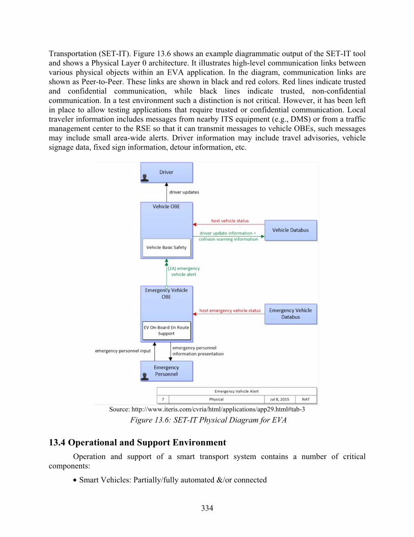
334

Transportation (SET-IT). Figure 13.6 shows an example diagrammatic output of the SET-IT tool and shows a Physical Layer 0 architecture. It illustrates high-level communication links between various physical objects within an EVA application. In the diagram, communication links are shown as Peer-to-Peer. These links are shown in black and red colors. Red lines indicate trusted and confidential communication, while black lines indicate trusted, non-confidential communication. In a test environment such a distinction is not critical. However, it has been left in place to allow testing applications that require trusted or confidential communication. Local traveler information includes messages from nearby ITS equipment (e.g., DMS) or from a traffic management center to the RSE so that it can transmit messages to vehicle OBEs, such messages may include small area-wide alerts. Driver information may include travel advisories, vehicle signage data, fixed sign information, detour information, etc.

Source: http://www.iteris.com/cvria/html/applications/app29.html#tab-3

Figure 13.6: SET-IT Physical Diagram for EVA

13.4 Operational and Support Environment

Operation and support of a smart transport system contains a number of critical components:

• Smart Vehicles: Partially/fully automated &/or connected

335

• Smart Infrastructure: Wide geographic distribution, reliable up-time, & data “portals” for traffic managers

• Smart Management: Highly integrated TxDOT traffic management center, tollway authorities, and law enforcement

These components cross previously separate stakeholder boundaries, and involve both

public and private organizations and interests. The operational and support environments for an OBE will be vastly different for those of an RSE, etc.

13.5 Operational Scenarios

The operational scenarios described below show how various users of a smart transport system might experience CAV technologies, such as emergency vehicle alerts, wrong-way driver notifications, and road maintenance data over wide geographic areas. The concept of a smart transport system is a very broad topic and covers many use cases, applications, and entities. The scenarios below are just a sampling of use cases that were included in the scope of this phase of work.

13.5.1 Emergency Vehicle Alert (EVA)

Emergency vehicles, within the context of the current Connected Vehicle environment, include police vehicle, ambulances, fire trucks, first responders, as well as maintenance and utility vehicles in certain situations, such as snow plows, road striping vehicles, and tow trucks. A loose definition of ‘emergency vehicles’ in this context is any vehicle that is expected, and legally, performing an unusual behavior on a typical roadway. An unusual behavior may be any non-standard traffic maneuver, such as traveling at higher or lower speed than expected for the roadway, traveling in a different direction than defined traffic flow—either crossing a roadway or driving upstream against traffic, or any other action that would benefit the safety and efficiency of themselves and nearby vehicles by providing information on the nature of their movement or intentions.

Emergency vehicles, like ambulances, police cars, fire trucks, and construction vehicles, broadcast out an EVA when they are activated, which can be received by nearby CVs. A driver, or an automated vehicle, that receives this alert could then make informed decisions about how to react, such as slowing down or pulling over. An implementation might look like what is shown in Figure 13.7, where a CV receives an EVA from an ambulance that is approaching from behind, and is currently a certain distance away. As the vehicle gets closer, the decision could be made to pull over to allow the ambulance to pass.

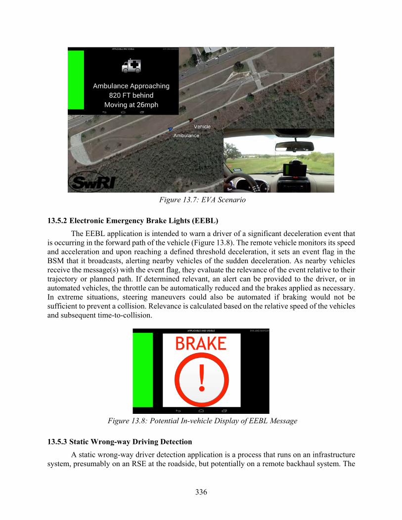
336

Figure 13.7: EVA Scenario

13.5.2 Electronic Emergency Brake Lights (EEBL)

The EEBL application is intended to warn a driver of a significant deceleration event that is occurring in the forward path of the vehicle (Figure 13.8). The remote vehicle monitors its speed and acceleration and upon reaching a defined threshold deceleration, it sets an event flag in the BSM that it broadcasts, alerting nearby vehicles of the sudden deceleration. As nearby vehicles receive the message(s) with the event flag, they evaluate the relevance of the event relative to their trajectory or planned path. If determined relevant, an alert can be provided to the driver, or in automated vehicles, the throttle can be automatically reduced and the brakes applied as necessary. In extreme situations, steering maneuvers could also be automated if braking would not be sufficient to prevent a collision. Relevance is calculated based on the relative speed of the vehicles and subsequent time-to-collision.

Figure 13.8: Potential In-vehicle Display of EEBL Message

13.5.3 Static Wrong-way Driving Detection

A static wrong-way driver detection application is a process that runs on an infrastructure system, presumably on an RSE at the roadside, but potentially on a remote backhaul system. The

337

process utilizes an operator-defined map of an area that is to be monitored. The map may be in various forms, but two common examples include a geo-bounded region with a defined direction and a list of points that define one or more lane segments with an implied direction. The process receives BSMs from passing vehicles and each are checked against the available map to determine if they are traveling in the allowed/defined direction within an allowable heading tolerance. When a vehicle is detected driving the wrong way, the process can provide an alert out to the vehicle driving the wrong way, to other nearby vehicles to alert them, and to traffic management center operators and law enforcement personnel. An example illustration of potential in-vehicle alerts are shown in Figure 13.9.

Figure 13.9: CV WWD Messages Sent by RSE

13.5.4 Intelligent Message Propagation (IMP)

This CV application would enable vehicles or infrastructure devices (RSEs) to pass along (propagate) messages they have received, which would be very useful, for example, in a scenario where RSE coverage is sparse or otherwise unavailable, and would enable CVs to continue to be informed of important events without RSE coverage. V2V message propagation is also viable for this application. This application would be applicable over large geographic areas with many vehicles, enabling a message to rapidly move from vehicle-to-vehicle. The final use of the message would depend on the message content, and could be consumed by individual vehicles, for example in the case of a weather-related warning, or could be consumed by an RSE, for example in the case of a stranded motorist. In Figure 13.10, a simulated CV traffic system is shown with the effective DSRC range of vehicles shown in red and that of RSEs shown in green. This illustrates how a smart transport system could be enabled without a 100% coverage of RSEs, as long as there is sufficient market penetration of CVs.

338

Figure 13.10: Simulated CVs along I-410 in San Antonio Showing Potential for Message

Propagation Between RSEs

13.5.5 Road Condition Monitoring (RCM)

According to current estimates, potholes cause approximately $6.4 billion in damage annually, making timely detection and repair of degraded roadways a significant concern for citizens and governments alike. Current methods for detection of poor road conditions consist of manual surveying, which is limited by the available resources of a traffic management entity. While the prevalence of smartphones has increased the ability for individuals to report road condition issues, the use of CV communication protocols presents a unique opportunity to enable vehicles to identify regions of pavement that require immediate maintenance, and to observe trends in pavement conditions over time. The necessary technologies to accomplish this, such as accelerometers, GPS-based localization systems, and CV DSRC, are becoming more widely available, enabling new applications to be developed to enhance the collective situational awareness of the vehicles themselves, and of the traffic system as a whole.

One method for determining the condition of a roadway is by utilizing the incoming accelerometer and GPS data to quantify road roughness, which can be scaled across various spatial windows that reflect different aspects of road health. For example, a smaller spatial window will detect shorter term anomalies in road condition, such as might be caused by a pothole or piece of debris in the road, while a larger window will detect more general roughness on a segment of road, which may indicate road surface deterioration. Data that has been received by another vehicle or an RSE can be utilized to illustrate the road conditions across a broad geographic area, which can then be displayed graphically as shown in Figure 13.11.

339

Figure 13.11: Incident Data Sent to TxDOT

This data could be used by nearby vehicles to avoid routes with heavy damage, and could be used by TxDOT to gain a clear picture of immediate maintenance needs, as well as help to inform longer-term maintenance planning.

13.5.6 Dynamic Wrong-way Driving and Road Hazard Detection

Contrasting to the static wrong way driving detection process, a dynamic detection process does not require a predefined map to be input by an operator. Instead, the process is configured to listen to BSMs from vehicles within range and aggregate them into an understood map of the nominal driving patterns in the area. As more and more BSMs are received, it enforces the learned map and establishes a baseline that is used similar to an operator-defined static map or region of interest. BSMs are monitored against the map the same way as in a static wrong way driving detection process and wrong way driver alerts are generated in the same way. Because of the nature of the map generation, the process can quickly be applied to new areas and is only restricted by the RF coverage area of the RSE.

Additionally, subtler deviations from the nominal patterns can be detected and used to identify localized road hazards, such as debris on the road and potholes. Multiple sequences of BSMs that similarly deviate laterally from the learned lanes can provide useful information to roadway operators, with much less delay than waiting for users to report issues or for traditional sensors or detection methods. See Figure 13.12.

340

Figure 13.12: Smart Transport System Lane Learning

This chapter has explored a concept of operations (ConOps) that describes the goals and objectives of a system. These directly feed into design practices to meet user needs. ConOps are foundational for the design, test, deployment, and implementation of smart transport technologies, like CAVs, and serve as a resource for the development of engineering requirements and decision-making processes that facilitate deployment and evaluation of smart transport systems.

341

Chapter 14. Conclusions and Recommendations

Smart-driving technologies are changing the landscape of transportation. Significant mobility, safety and environmental benefits are anticipated from these technologies, which enable safer and more comfortable driving in general. However, in order to realize the maximum potential benefits for the overall transportation system in Texas, these technologies alone are not enough. Rather, policymaking and innovation in infrastructure and operations strategies, among other measures, are crucial.

The objectives of this project’s first phase were to develop and demonstrate a variety of smart-transport technologies, policies, and practices for Texas highways and freeways using AVs and CVs, smartphones, roadside equipment, and related technologies.

A series of conclusions and recommendations were developed during the initial project timeframe, partially in conjunction with TxDOT Projects 0-6847 and 0-6849, which go deeply into the traffic and safety impacts of C/AVs. In addition, a series of specific recommendations for TxDOT headquarters and divisions was developed based upon the legal analysis undertaken within this project, and the safety and crash analysis that TxDOT project 0-6849 assessed. These can be seen in Section 14.1.1.

The work’s products provide ideas and equipment for more efficient intersection, ramp, and weaving section operations for CAV operations, alongside a suite of behavioral and traffic-flow forecasts for Texas regions and networks under a variety of vehicle mixes (smart plus conventional, semi-autonomous versus fully autonomous, connected but not automated). The work provides rigorous benefit-cost assessments of multiple strategies that TxDOT may pursue to bring smarter, safer, more connected, and more sustainable ground transportation systems to Texas, in concert with auto manufacturers, technologists, and the traveling public. The effort supports proactive policymaking on vehicle and occupant licensing, liability, and privacy standards, as technologies become available and travel behaviors change.

Chapter 3’s survey results reflect the current perceptions of Americans (and more specifically, of Texans). As the public learns more about CAVs and more people gain familiarity with these technologies, perceptions and potential behavioral responses are apt to change, in some cases rapidly. For example, a large proportion (more than 50%) of individuals who do not want to pay anything for advanced automation technologies may change their perspectives, as the technology becomes proven and they see their neighbors, friends, and co-workers adopt AVs with great success. Alternatively, a well-publicized catastrophe, such as a multi-vehicle, multi-fatality cyber-attack, could set adoption rates back years. As such, more survey work is required elsewhere in the U.S. and other countries, and over time. This is a dynamic stage for an important impending technological shift. Knowledge of the underlying factors across geographies and over time will be important in helping all relevant actors (the public, businesses, regulators, and policymakers) coordinate to enable cost-effective, environmentally sensitive, and operationally efficient transformation of the transportation system.

Chapter 4’s results suggest that advanced CAV technologies may reduce current crash costs by at least $390 billion per year, including pain and suffering damages, and other non-economic costs. These results rely on the three different effectiveness scenarios with a 100% market penetration rate of all CV- and AV-based safety technologies.

Of the eleven safety applications, the one with the greatest potential to avoid or mitigate crashes, but not yet on the market, is Full Automation of one’s vehicle. A currently available technology, AEB, also offers substantial safety rewards, with an estimated economic savings of

342

$23.5 to $100 billion each year, assuming full adoption across the U.S., along with current crash counts. Among the CV-based safety applications, CICAS is estimated to offer the greatest economic and comprehensive cost savings. Overall, AV-based technologies are expected to offer far more safety benefits than CV-based technologies, as expected, since automation proactively avoids human errors during travel, rather than simply warning human drivers about possible conflicts.

There is little doubt that various CAV technologies will offer significant safety benefits to transportation system users. However, the actual effectiveness of these technologies will not be known until sufficient real-world data have been collected and analyzed.

As Chapter 12 concludes, CAVs will transform our economy and change the landscape of almost every industry. Although some sectors will be more significantly affected than others, ripple effects will be felt throughout most, if not all industries. The technology still has a long road of development ahead and market penetration rates will define the size of the impact of driverless vehicles. With the assumption that AVs will eventually become pervasive, or at least hold a large share of the automotive market, it is assured that they will have a strong economic impact, potentially as much as $1.3 trillion or more. In order to prepare for this revolution, we must be aware of the potential effects so that we can alter our established systems to accommodate these changes. Change is coming, and we must be prepared to adapt.

14.1 Specific Recommendations for TxDOT Headquarters and Divisions

14.1.1 Shaping Legislative Policy on CAVs

There is a great deal of uncertainty regarding the current position of state and federal laws concerning CAV use. Various organizations and OEMs (original equipment manufacturers) are researching and developing CAV technologies, but there is little oversight on the extent to which CAVs can be tested and operated for private use on Texas roadways. Because of TxDOT’s status as the primary transportation agency in the state, the organization can play an important role in shaping the legislative policy for the testing and deployment of CAVs. Though taking no legislative action is a possible option, being proactive in shaping policy will help Texas reap the potential safety and operational benefits expected of CAVs to a greater extent and at a faster pace. Some of the legislative questions that TxDOT should urge the legislature to address include:

• Creating a single agency point person, situated within TxDOT, who has authority and credibility to coordinate among various state and local agencies within Texas. This would also assist in ‘preparing government’ for the transition to this new driving paradigm.

o The research team suggests that the point person should have a minimum number of years of experience at TxDOT, preferably at division/district deputy level;

o A secondary recommendation is that TxDOT OGC should appoint a staffer to assist the TxDOT point person, and to provide a liaising link to the Attorney General’s office for clarification on any state-level legal issues.

• Setting standards for testing and development of CAVs

• Legally defining the “operator” of a CAV

• Establishing rules for intensive use of truck platooning

343

• Addressing privacy and security questions stemming from CAV use

• Answering liability questions that arise from CAV adoption

• Advancing broader public goals in CAV innovation

14.1.2 Short-Term Practices

• Appoint a TxDOT CAV point person, who has authority and credibility as the state’s point person on CAV issues, challenges, outreach and education.

• Establish a department-wide working group to:

o Coordinate and provide to the Legislature technical advice as well as recommendations for legislative policy making and changes or additions to the Texas Transportation Code and Texas Administrative Code applicable to CAVs;

o Oversee continuing research and testing needed to assess the technically feasible and economically reasonable steps for TxDOT to pursue over time, with emphasis on those actions that will encourage early CAV market penetration;

o Create and update annually a CAV policy statement and plan;

o Create and update annually a policy statement and plan for non-CAV vehicle support and operations during the transition to CAVs; and

o Coordinate CAV issues with AASHTO, other states, Transportation Research Board (TRB) committees, the Texas Department of Motor Vehicles, and the Texas Department of Public Safety.

• The Traffic Operations Division (TRF), in coordination with other divisions, the districts, and other stakeholders, should establish and lead a team to:

o Oversee research and testing on additional or changed traffic control devices and signage that will enhance the operations of CAVs and reduce liability issues;

o Coordinate with industry in the short term on basic items in the MUTCD that are proving challenging in CAV development and deployment, such as sensor-compatible lane striping, road buttons, and machine-readable signage;

o Monitor and oversee development of cooperative intersection collision avoidance system technology and assist in test deployments on Texas highways and major arterial roads; and

o Monitor cooperative-adaptive cruise control and emergency stop device deployment and assess what steps TxDOT will need to take to assist in extending and translating this technology into throughput, such as improved platooning on trunk routes.

• The Transportation Planning and Programming (TPP) Division, in coordination with other divisions, the districts, and other stakeholders, should establish and lead a team to:

o Develop and continuously maintain a working plan for facilitating early adaptors of CAV technology, in particular the freight and public transportation industries;

344

o Identify and begin planning with MPOs for the impacts of expected additional VMT driven by CAV adoption, particularly for assessing impacts on conformity demonstrations in non-attainment areas of the state;

o Begin assessment for and development of a series of TxDOT-recommended VMT management and control incentives for responding to the likely CAV-induced VMT increases; and

o In coordination with the Public Transportation Division (PTN), begin to monitor and assess the impacts of SAVs on the department.

14.1.3 Mid-Term Practices

• The department-wide working group should continue to:

o Create and update annually the CAV policy statement and plan;

o Create and update annually the plan for non-CAV vehicle support and operations during the transition to CAVs;

o Coordinate CAV issues with AASHTO, other states, TRB committees, the Texas Department of Motor Vehicles, and the Texas Department of Public Safety; and

o Coordinate and provide to the Legislature technical advice as well as recommendations for legislative policy making and changes or additions to the Texas Transportation Code and Texas Administrative Code.

• The TRF Division, in coordination with other divisions, the districts, and other stakeholders, should:

o Continue research and testing for CAV-enabled smart intersections, expanding from off-road test facilities to actual intersections;

o Initiate research and testing for CAV-appropriate lane management operations, initially for platooning and CAV-only lanes;

o Expand CAV-compatible traffic control device research and testing specific to construction zone, detour, and nighttime operations; and

o In cooperation with the engineering design divisions and the Maintenance Division (MNT), begin updating the various TxDOT manuals that will be impacted by CAVs.

• The TPP Division, in coordination with other divisions, the districts, and other stakeholders, should:

o Research, test, and recommend incentives (for example, micro-tolling, time of day operations restrictions, etc.) for the control of congestion as well as increased VMT induced by CAVs;

o In coordination with PTN and local governments, assess the impact of CAVs in public transportation operations, leading to recommendations appropriate to the Department’s goal of congestion relief; and

o Begin research and testing of area-wide traffic demand management operations made possible by CAV technology.

345

14.1.4 Long-Term Practices

• TxDOT’s department-wide working group should continue to:

o Create and update annually the CAV policy statement and plan;

o Create and update annually the plan for non-CAV vehicle support and operations during the transition to CAVs;

o Coordinate CAV issues with AASHTO, other states, TRB committees, the Texas Department of Motor Vehicles, and the Texas Department of Public Safety; and

o Coordinate and provide to the Legislature technical advice as well as recommendations for legislative policy making and changes or additions to the Texas Transportation Code and Texas Administrative Code.

• TRF and TPP should continue steps needed to identify the optimal traffic demand management strategies that are economically feasible and environmentally compliant, giving particular thought to centralized and automated allocation of routing and timing, as well as required use of SAVs operated to minimize VMT.

• TRF, in coordination with the other engineering design divisions (Design Division, Bridge Division) and MNT, should research, test, and ultimately adopt changes to the department manuals optimized for CAV/SAV operations.

• The engineering design divisions should research, test, and ultimately adopt roadway design elements that allow high-speed, but safe, CAV roadway operations in rural and uncongested suburban areas.

• Finally, TPP, in coordination with TRF, PTN, and the engineering design divisions, should develop and recommend a series of options to the TxDOT administration and Texas Transportation Commission for aggressive traffic demand management in the major metro areas and along congested trunk routes.

346

References

Abdulhai, B. & Look, H. (2003) Impact of Dynamic and Safety-Conscious Route Guidance. Journal of Transportation Engineering, 129(4), 369-376.

ABI Research (2013) Half of new vehicles shipping in North America to have driverless, robotic capabilities by 2032. Retrieved from:https://www.abiresearch.com/press/half-of-new-vehicles-shipping-in-north-america-to-/ (July 10, 2015).

Abou-Senna, H. and E. Radwan (2013) VisSim/MOVES integration to investigate the effect of major key parameters on CO2 emissions. Transportation Research Part D: Transport and Environment, 21, 39 – 46.

Alexander, D. and Gartner, J. (2014) Self-driving vehicles, advanced driver assistance systems, and autonomous driving features: Global market analysis and forecasts. Navigant Consulting, Inc. Retrieved from: https://www.navigantresearch.com/research/autonomous-vehicles (June 21, 2015).

American Automobile Association (2015) Your Driving Costs. http://exchange.aaa.com/wp-content/uploads/2015/04/Your-Driving-Costs-2015.pdf.

Amirjamshidi, G. and M.J. Roorda (2015) Development of simulated driving cycles for light, medium, and heavy duty trucks: Case of the Toronto Waterfront Area. Transportation Research Part D: Transport and Environment, 34, 255 – 266.

Anderson, James, Nidhi Kalra, Karlyn Stanley, Paul Sorensen, Constantine Samaras, and Oluwatobi Oluwatola (2014) Autonomous Vehicle Technology: A Guide for Policymakers RAND: Santa Monica, CA.

Anderson, Ross P. and Milutinovic, Dejan (2014) A stochastic approach to Dubins vehicle tracking problems. IEEE Transactions on Automatic Control. 59.10, 2801 – 2806.

Australian Broadcast News (ABC) (2015) First Driverless Car Trials in Southern Hemisphere to be held in Adelaide, Coinciding with International Conference. URL: http://www.abc.net.au/news/2015-07-21/driverless-car-trials-held-in-adelaide/6636334 on October 27, 2015.

Automotive Digest (2014) NHTSA calls for V2V technology in models built after 2020. Retrieved from: http://automotivedigest.com/2014/08/nhtsa-eyes-half-million-crashes-prevented-v2v-technology/ (July 19, 2015).

Autonomos Labs (n.d.) Frequently Asked Questions. Not dated. URL: http://autonomos-labs.com/faq/ on October 23, 2015.

Bansal, P., Kockelman, K. (2015) Forecasting Americans’ Long-term Adoption of Connected and Autonomous Vehicle Technologies. Under review for publication in Transportation

347

Research Part A, and available at http://www.ce.utexas.edu/prof/kockelman/public_html/TRB16CAVTechAdoption.pdf.

Bansal, P., Kockelman, K., and Singh, A. (2016) Assessing Public Opinions of and Interest in New Vehicle Technologies: An Austin Perspective. Transportation Research Part C 67: 1-14.

Beckmann, M. J., McGuire, C. B., Winston, C. B. (1956) Studies in the Economics of Transportation. Yale University Press: New Haven, CT.

Begg, D. (2014) A 2050 vision for London: What are the implications of driverless transport. Commissioned by Clear Channel http://www.transporttimes.co.uk/Admin/uploads/64165-transport-times_a-2050-vision-for-london_aw-web-ready.pdf

Benko, M., & Smith, L. (2008) Congestion Pricing: What is It? Community Transportation Association. http://web1.ctaa.org/webmodules/webarticles/articlefiles/Congestion_Pricing.pdf

Benning, Tom (2013) More North Texas Highways Slated to Feature Ban on Trucks in Left Lane. (June 3, 2013) The Dallas Morning News Transportation Blog. URL: http://transportationblog.dallasnews.com/2013/06/more-north-texas-highways-slated-to-feature-ban-on-trucks-in-the-left-lane.html/ on October 23, 2015.

Berry, I. (2010) The Effects of Driving Style and Vehicle Performance on the Real-World Fuel Consumption of U.S. Light-Duty Vehicles. Department of Mechanical Engineering and the Engineering Systems Division. Massachusetts Institute of Technology.

Bierlaire, M. (2003) BIOGEME: A free package for the estimation of discrete choice models. Proceedings of the 3rd Swiss Transportation Research Conference, Ascona, Switzerland.

Bierstedt, J., Gooze, A., Gray, C., Peterman, J., Raykin, L., and Walters, J. (2014) Effects of next-generation vehicles on travel demand and highway capacity. Technical report. Fehr & Peers Transportation Consultants. Retrieved from: http://orfe.princeton.edu/~alaink/Papers/FP_NextGenVehicleWhitePaper012414.pdf (June 22, 2014).

Bishop, R. (2005) Intelligent Vehicle Technology and Trends. Norwood, MA: Artech House.

Blincoe, L. J., Miller, T. R., Zaloshnja, E., Lawrence, B. A. (2015) The economic and societal impact of motor vehicle crashes, 2010 (Revised). Report No. DOT HS 812 013. Washington, DC: National Highway Traffic Safety Administration.

Boske, L. and R. Harrison (2014) “Transportation Policy Brief No. 2: Autonomous Vehicles in Texas.” Prepared for TxDOT, Project No. 0-6581, by the Center for Transportation Research and Lyndon B. Johnson School of Public Affairs. Accessed at http://library.ctr.utexas.edu/ctr-publications/policy/0-6581_task19-2.pdf on October 17, 2015.

348

Braess, P. D. (1968) Über ein Paradoxon aus der Verkehrsplanung. Unternehmensforschung, 12(1), 258 – 268.

Brookings Institution (2014) Products Liability and Driverless Cars: Issues and Guiding Principles for Legislation. http://www.brookings.edu/research/papers/2014/04/products-liability-driverless-cars-villasenor

Burns, L. D., Jordan, W. C., & Scarborough, B. A. (2013) Transforming Personal Mobility. The Earth Institute, Columbia University.

Burris, M., & Sullivan, E. (2006) Benefit-Cost Analysis of Variable Pricing Projects: QuickRide HOT Lanes. Journal of Transportation Engineering, 132(3), 183-190.

California Department of Motor Vehicles (DMV) (2012) Autonomous Vehicles in California: Deployment of Autonomous Vehicles for Public Operation, Accessed at http://apps.dmv.ca.gov/about/lad/pdfs/auto_veh2/adopted_txt.pdf on October 23, 2015.

California State Legislature (2012) Senate Bill (SB) 1298, Chapter 570. Filed with the Secretary of State on September 25, 2012. https://leginfo.legislature.ca.gov/faces/billNavClient.xhtml?bill_id=201120120SB1298 Accessed on October 18, 2015.

Casley, S. V., Jardim, A. S., and Quartulli, A. M. (2013) A Study of Public Acceptance of Autonomous Cars. Bachelor of Science thesis. Worcester Polytechnic Institute, Worcester, MA, USA. Retrieved from: http://bit.ly/2gSOozZ (March 8, 2015).

Chapin III, F.S., Grimm, N.B., Bierwagen, B., Gonzalez, P., Groffman, P.M., Luo, Y., Melton, F., Nadelhoffer, K., Pairis, A., Raymond, P.A. and Schimel, J. (2013) The impacts of climate change on ecosystem structure and function. Frontiers in Ecology and the Environment 11 (9): 474 – 482.

Chen, D., Kockelman, K., and Hanna, J. (2016) Operations of a Shared, Autonomous, Electric Vehicle (SAEV) Fleet: Implications of Vehicle & Charging Infrastructure Decisions. Proceedings of the 95th Annual Meeting of the Transportation Research Board, and available at http://www.ce.utexas.edu/prof/kockelman/public_html/TRB16SAEVs100mi.pdf .

Childress, S., B. Nichols, B. Charlton, S. Coe (2014) Using an Activity-Based Model to Explore Possible Impacts of Automated Vehicles. Puget Sound Regional Council. Retrieved from: https://psrc.github.io/attachments/2014/TRB-2015-Automated-Vehicles-Rev2.pdf

Cisco Systems (2013) Cisco Customer Experience Research: Automotive Industry. Cisco Systems. Retrieved from: https://www.cisco.com/web/about/ac79/docs/ccer_report_manufacturing.pdf (September 13, 2015)

349

Citi GPS: Global Perspectives & Solutions (2014) The car of the future: Transforming mobility as we know it. Retrieved from: https://www.citivelocity.com/citigps/ReportSeries.action?recordId=27 (June 28, 2014).

CityMobile2 (2015) Cities Demonstrating Automated Road Passenger Transport. URL: http://www.citymobil2.eu/en/About-CityMobil2/Overview/ on October 23, 2015.

CityMobile2 (2015) La Rochelle. Large Scale Demonstration. URL: http://www.citymobil2.eu/en/City-activities/Large-Scale-Demonstration/La-Rochelle/ on October 23, 2015.

CMAP (2015) Regional Transportation Performance Measurement. Retrieved from http://www.cmap.illinois.gov/mobility/roads/cmp/performance-measurement.

Conklin, C. A., Bahler, S. J., Belmore, K. L., Hallenbeck, M., Ishimura, J., Schnell, G. M., But, A. (2013) Transportation Management Center Data Capture for Performance and Mobility Measures Guidebook. Washington, DC: U.S. Department of Transportation.

Continental (2015) Continental Mobility Study 2015. Retrieved from: https://www.conti-online.com/www/download/pressportal_com_en/themes/initiatives/channel_mobility_study_en/ov_mobility_study2015_en/download_channel/mobistud2015_praesentation_en.pdf (March 7, 2015).

Crane, D.A.., Logue, K.D., and Pilz, B.C. (2016) A Survey of Legal Issues Arising from the Deployment of Autonomous and Connected Vehicles. Michigan Law: Public Law and Legal Theory Research Paper Series, Paper No 16-015.

Daganzo, C. F. (1998) Queue spillovers in transportation networks with a route choice. Transportation Science, 32(1), 3 – 11.

Danise, A. (2015) Women say no thanks to driverless cars, survey finds; Men say tell me more. Retrieved from NerdWallet: http://www.nerdwallet.com/blog/insurance/2015/06/09/survey-consumer-fears-self-driving-cars/ (Setember 21, 2015).

Danna, S., Mori, K., Vela, J., & Ward, M. (2012) A Benefit-Cost Analysis of Road Pricing in Downtown Seattle. Evans School Review. https://depts.washington.edu/esreview/wordpress/wp-content/uploads/2012/12/ESR-2012-A-Benefit-Cost-Analysis-of-Road-Pricing-in-Downtown-Seattle.pdf

Davidson, Peter and Anabelle Spinoulas (2015) Autonomous Vehicles - What Could This Mean for the Future of Transport, AITPM 2015 National Conference at 3.

Davis, S., S. Diegel, and R. Boundy (2009) Transportation Energy Data Book: Edition 28, ORNl-6984, Oak Ridge National Laboratory, Oak Ridge, Tennessee.

Dial, Robert B. (2006) A path-based user-equilibrium traffic assignment algorithm that obviates path storage and enumeration. Transportation Research Part B, 40.10, 917 – 936.

350

Douma, Frank and Sarah Aue Palodichuk (2012) Criminal Liability Issues Created by Autonomous Vehicles, 52 Santa Clara L. Rev. 1157.

Dresner, K. and Stone, P. (2005) Multiagent traffic management: An improved intersection control mechanism. Proceedings of the fourth international joint conference on Autonomous agents and multiagent systems, 471 – 477, ACM.

Dresner, K. and Stone, P. (2008) A multiagent approach to autonomous intersection management. Journal of Artificial Intelligence Research, vol 31, 591–656.

Duffy, Sophia and Jamie Patrick Hopkins (2013) Sit, Stay, Drive: The Future of Autonomous Car Liability. 16 SMU Sci. & Tech L. Rev 453 (2013) at 118-122.

Economic Commission for Europe: Inland Transport Committee (1968) Convention on Road Traffic. URL: http://www.unece.org/fileadmin/DAM/trans/conventn/crt1968e.pdf on October 23, 2015.

Electronic Privacy Information Center (2013) Comments to the National Highway Traffic Safety Administration: Federal Motor Vehicle Safety Standards, Event Data Recorders. URL: https://epic.org/privacy/edrs/EPIC-Coal-NHTSA-EDR-Cmts.pdf on October 23, 2015.

Elvik, R., & Vaa, T. (1997) The Handbook of Road Safety Measures. Emerald Group Publishing Limited, Bingley, UK

Environmental Protection Administration (EPA) (2012) Joint Technical Support Document: Final Rulemaking for 2017-2025 Light-Duty Vehicle Greenhouse Gas Emission Standards and Corporate Average Fuel Economy Standards. U.S. Environmental Protection Agency (EPA) Ann Arbor, MI.

Environmental Protection Administration (EPA) (2013) Dynamometer Drive Schedules. Cited 2014 March 3rd, Available from: http://www.epa.gov/nvfel/testing/dynamometer.htm.

Examiner (2015). TxDOT Tracks Drivers to Mine Data Without their Consent. June 2, 2015. URL: http://www.examiner.com/article/txdot-tracks-drivers-to-mine-data-without-their-consent on October 23, 2015.

Fagnant, D. J., & Kockelman, K. M. (2014) The travel and environmental implications of shared autonomous vehicles, using agent-based model simulations. Transportation Research Part C: Emerging Technologies, 40, 1-13.

Fagnant, D. J., and Kockelman, K. (2015) Preparing a nation for autonomous vehicles: opportunities, barriers and policy recommendations. Transportation Research Part A: Policy and Practice, 77: 167-181.

Fagnant, D. J., and Kockelman, K. M. (2015) Dynamic ride-sharing and optimal fleet sizing for a system of shared autonomous vehicles. Proceedings of the 94th Annual Meeting of the Transportation Research Board and submitted for publication in Transportation.

351

Fagnant, D. J., Kockelman, K., and Bansal, P. (2015) Operations of a shared autonomous vehicle fleet for the Austin, Texas market. Transportation Research Record, 2536: 98-106.

Farzaneh, M., Zietsman, J., Lee, D.W., et al. (2014) Texas-Specific Drive Cycles and Idle Emissions Rates for Using with EPA’s MOVES Model – Final Report. TxDOT Report 6629-1. http://d2dtl5nnlpfr0r.cloudfront.net/tti.tamu.edu/documents/0-6629-1.pdf

Federal Highway Administration (FHWA) (2015) Multi-Modal Intelligent Traffic Signal Systems (MMITSS) Impacts Assessment. http://ntl.bts.gov/lib/55000/55700/55710/MMITSS_IA_REPORT_0811_v1.4.pdf

Federal Trade Commission (2014) Comment: Advance Notice of Proposed Rulemaking Regarding Federal Motor Vehicle Safety Standards: Vehicle-to-Vehicle (V2V), Docket No. NHTSA-2014-0022, Oct. 20, 2014, URL: http://bit.ly/2gG5DA1

Fellows, N. T., & Pitfield, D. E. (2000) An economic and operational evaluation of urban car-sharing. Transportation Research Part D, 5, 1-10.

Florida Department of Highway Safety and Motor Vehicles (DHSMV) (2014) “Autonomous Vehicle Report.” URL: http://www.flhsmv.gov/html/HSMVAutonomousVehicleReport2014.pdf

Ford, J.D. (2012) Indigenous health and climate change. American Journal of Public Health, 102.7, 1260 – 1266.

Froomkin, A. Michael (2009) Government Data Breaches, 24 Berkeley Tech. L.J. 1019.

Funkhouser, Kevin (2013) Paving the Road Ahead: Autonomous Vehicles, Products Liability, and the Need for a New Approach, 2013 Utah L. Rev. 437

Gardner, Lauren, Bar-Gera, Hillel, and Boyles, Stephen (2013) Development and comparison of choice models and tolling schemes for high-occupancy/toll (HOT) facilities. Transportation Research Part B, 55, 142 – 153.

Gardner, Lauren, Boyles, Stephen, Bar-Gera, Hillel, and Tang, Kelly (2015) Robust tolling schemes for high-occupancy/toll (HOT) facilities under variable demand. Transportation Research Part B, 2450, 152 – 162.

Glancy, D.J., Peterson, R.W., Graham, K.F. (2015) (pre-publication draft issued in spring 2016). A Look at the Legal Environment for Driverless Vehicles. NCHRP Legal Research Digest 63. Transportation Research Board Washington: D.C.

Glancy, Dorothy (2012) Privacy in Autonomous Vehicles. Santa Clara Law Review 52, 1171-1238

Glancy, Dorothy (2014) Sharing the Road: Smart Transportation Infrastructure, 41 Fordham Urb. L.J. 1617.

352

Glaskin, Max (2014) Safe and Secure, Vision Zero International 40.

Gosselin, Kurt, (2015) Navigating the Policy Landscape to Bring Autonomous Vehicle Legislation to your State, N.Y.U. J. of Legislation and Public Policy Quorum 85.

Government Accountability Office (GAO) (2013) Intelligent Transportation Systems: Vehicle-to-Vehicle Technologies Expected to Offer Safety Benefits but A Variety of Deployment of Challenges Exist. GAO Report 14-03, (Nov. 1, 2013). Accessed at http://www.gao.gov/products/GAO-14-13 on October, 23, 2015.

Government Accountability Office (GAO) (2015) Intelligent Transportation Systems: Vehicle-to-Vehicle Technologies Expected to Offer Safety Benefits but A Variety of Deployment of Challenges Exist. GAO Report 15-775. Accessed at http://www.gao.gov/products/GAO-15-775 on October, 27, 2015.

Government Accountability Office (GAO) (2016) Report Number GAO 16-350. Vehicle Cybersecurity: DOT and Industry Have Efforts Underway, but DOT Needs to Define Its Role in Responding to a Real-world Attack. URL http://www.gao.gov/assets/680/676064.pdf

Government Accountability Office (GAO) (2012) GAO-12-903, Mobile Device Location Data: Additional Federal Action Could Help Protect Consumer Privacy.

Government of Japan: Cabinet Office (JCSTI) (2014) Workshop on Connected and Automated Driving Systems. November 2014. URL: http://www8.cao.go.jp/cstp/gaiyo/sip/workshop201411.html on October 23, 2015.

Government of Japan: Ministry of Economy, Trade and Industry (2014) Meti Journal March Issue. Autonomous Driving: Creating an Optimal Relationship Between People and Automobiles. URL: http://www.meti.go.jp/english/publications/pdf/journal2014_03a.pdf on October 23, 2015.

Government of Japan: Ministry of Land, Infrastructure, Transport, and Tourism (MLIT) (2012) ITS Initiatives in Japan. URL: http://www.mlit.go.jp/road/ITS/pdf/ITSinitiativesinJapan.pdf on (October 23, 2015).

Government of Ontario (2013) Regulatory Registry. A Pilot Project to Safety Test Autonomous Vehicles. December 17, 2013. Registry Number 011-9707. URL: http://www.ontariocanada.com/registry/showAttachment.do?postingId=14802&attachmentId=22912

Government of South Australia: Attorney General’s Department (2015) Motor Vehicles (Trials of Automotive Technologies) Amendment Bill 2015. HA GP 334-1 OPC 112. September 23, 2015. URL: http://bit.ly/2fA5iml on October 27, 2015

Government of South Australia: Department of Planning, Transport and Infrastructure (DPTI) (2015) South Australia Leads Nation on Driverless Car Legislation. September 22, 2015. Accessed: at http://dpti.sa.gov.au/news/?a=177492 on October 27, 2015.

353

Greene, W. H. (2012) Econometric Analysis (7th edition). Boston: Pearson Education.

Grovdahl, D. L., & Hill, E. T. (2000) Regional Planning and Intelligent Transportation Systems: Effects on Land Use and Society. ITE Journal, March 2000, 34-38.

Han, Darren and Yang, Hai (2009) Congestion pricing in the absence of demand functions. Transportation Research Part E: Logistics and Transportation Review 45.1, 159 – 171.

Harding, J., Powell, G., R., Yoon, R., Fikentscher, J., Doyle, C., Sade, D., Lukuc, M., Simons, J., Wang, J. (2014) Vehicle-to-Vehicle Communications: Readiness of V2V Technology for Application. Report No. DOT HS 812 014. Washington, DC: National Highway Traffic Safety Administration.

Harrop, P. and Das, R. (2015) Autonomous Vehicles: Land, Water, Air 2015-2035. Retrieved from: http://www.prnewswire.com/news-releases/autonomous-vehicles-land-water-air-2015-2035-300096548.html (June 28, 2014).

Hars, A. (2014) Autonomous vehicle roadmap: 2015-2030. Driverless Future website. Retrieved from: http://www.driverless-future.com/?p=678 (June 29, 2015).

Howard, D. and Dai, D. (2013) Public perceptions of self-driving cars: The case of Berkeley, California. Presented at the 93rd Annual Meeting of Transportation Research Board, Washington DC. Retrieved from: https://www.ocf.berkeley.edu/~djhoward/reports/Report%20-%20Public%20Perceptions%20of%20Self%20Driving%20Cars.pdf (September 20, 2015).

Hutton, P. (2014) A driverless future? Retrieved from: http://thinkinghighways.com/a-driverless-future/.

IHS Automotive (2014) Emerging technologies: Autonomous cars—not if, but when. Retrieved from: http://collision.honda.com/ihs-automotive-forecasts-54-million-self-driving-cars-used-globally-by-2035-#.VbVnkPlViko.

Insurance Information Institute (2015) Self-Driving Cars and Insurance. URL: http://www.iii.org/issue-update/self-driving-cars-and-insurance.

Insurance Institute for Highway Safety (IIHS) (2016) Crashes avoided. Status Report 51 (1): 2-3. http://www.iihs.org/externaldata/srdata/docs/sr5101.pdf

International Organization for Standards (ISO) (2015) ISOfocus: Issue 106, September-October 2014, URL: http://www.iso.org/iso/isofocus_106.pdf on October 23, 2015.

Ipsos MORI (2014) Ipsos MORI Loyalty Automotive Survey. Retrieved from: http://bit.ly/2fNNPFB (September 12, 2015).

ITS International (2015) Motor insurance for autonomous vehicles will shift from drivers to OEMs. URL: http://bit.ly/2gG3Jja

354

J.D. Power (2012) Vehicle owners show willingness to spend on automotive infotainment features. Retrieved from: http://www.jdpower.com/sites/default/files/2012049-uset.pdf (March 10, 2015).

J.D. Power (2015) 2015 U.S. Tech Choice Study. Retrieved from: http://www.jdpower.com/sites/default/files/2015044%20Tech%20Choice%20Study%20%28FINAL%29.pdf (August 12, 2015).

Jermakian, J.S. (2011) Crash Avoidance Potential of Four Passenger Vehicle Technologies. Accident Analysis & Prevention 43, 732 – 740.

Joksimovic, Dusica, Bliemer, Michael C. J., and Bovy, Piet H. L. (2005) Optimal toll design problem in dynamic traffic networks with joint route and departure time choice. Transportation Research Record, No. 1923, 61 – 72. DOI: 10.3141/1923-07

Jonas, A., S. C. Byrd, R. Shankar, and M. Ono (2014) Nikola’s Revenge: TSLA’s New Path of Disruption. Morgan Stanley & Co., LLC.

Kalra, Nidhi, James M. Anderson, and Martin Wachs (2009) Liability and Regulation of Autonomous Vehicle Technologies. California PATH Research Report. https://merritt.cdlib.org/d/ark:%252F13030%252Fm55x29z8/1/producer%252FPRR-2009-28.pdf

Karush, William (1939) Minima of functions of several variables with inequalities as side constraints. PhD thesis, Masters thesis, Department of Mathematics, University of Chicago.

Kim, Moon K.; Heled, Yaniv; Asher, Isaac; Thompson, Miles (2014) Comparative Analysis of Laws on Autonomous Vehicles in the U.S. and Europe. AUVSI’s Unmanned Systems Conference, Orlando, Florida.

Kohler, William and Alex Colbert-Taylor (2015) Current Law and Potential Legal Issues Pertaining to Automated, Autonomous and Connected Vehicles Santa Clara High Tech. L. J. 31, 99.

KPMG (2013) Self-driving cars: Are we ready? Retrieved from: http://www.kpmg.com/US/en/IssuesAndInsights/ArticlesPublications/Documents/self-driving-cars-are-we-ready.pdf (March 11, 2015).

Kuhn, H. W., Tucker, A. W. (1951) Nonlinear Programming. Proceedings of the Second Berkeley Symposium on Mathematical Statistics and Probability 481 – 492, Berkeley, CA, University of California Press.

Kurzweil (2012) A French Autonomous Car. (January 13, 2012). Accessed at http://www.kurzweilai.net/a-french-autonomous-car on October 23, 2015.

Kyriakidis, M., Happee, R., and De Winter, J. (2014) Public Opinion on Automated Driving: Results of an International Questionnaire Among 5,000 Respondents. Delft University of

355

Technology (working paper). Retrieved from: http://papers.ssrn.com/sol3/papers.cfm?abstract_id=2506579 (October 15, 2014).

Laslau, C., Holman, M., Saenko, M., See, K., and Zhang, Z. (2014) Set autopilot for profits: Capitalizing on the $87 billion self-driving car opportunity. Retrieved from: http://www.giiresearch.com/report/lux301508-set-autopilot-profits-capitalizing-on-87-billion.html (July 22, 2015).

Lenth, Danielle (2013) Chapter 570: Paving the Way for Autonomous Vehicles, 44 McGeorge L. Rev. 787.

Levinson, D. (2003) The value of advanced traveler information systems for route choice. Transportation Research Part C, 11, 75–87.

Levinson, D., Gillen, D., & Chang, E. (1999) Assessing the Benefits and Costs of Intelligent Transportation Systems: The Value of Advanced Traveler Information Systems. Berkeley, CA: UCB-ITS-PRR-99-20.

Litman, T. (2011) Measuring Transportation. Victoria Transport Policy Institute. http://www.vtpi.org/measure.pdf (March 1, 2011)

Litman, T. (2014) Autonomous vehicle implementation predictions. Victoria Transport Policy Institute. Retrieved from: http://www.vtpi.org/avip.pdf (March 10, 2015)

Litman, T. (2015) Autonomous vehicle implementation predictions. Victoria Transport Policy Institute. Retrieved from: http://www.vtpi.org/avip.pdf (March 10, 2015)

Litman, T. (2016) Evaluating Transportation Land Use Impacts. Victoria Transport Policy Institute. http://www.vtpi.org/landuse.pdf (August 24, 2016)

Little, C., & Wooster, J. (1994) IVHS and Environmental Impacts: Implications of the Operational Tests. National Policy Conference on Intelligent Transportation Systems and the Environment. Arlington, Virginia.

Liu, Bolan, Ai, Xiaowei, Liu, Pan, Zhang, Chuang, Hu, Xingqi, Dong, Tianpu (2015) Fuel Economy Improvement of a Heavy-Duty Powertrain by Using Hardware-in-Loop Simulation and Calibration. Energies (19961073). 8.9, 9878 – 9891.

Long, J. S., and Freese, J. (2006) Regression Models for Categorical Dependent Variables Using Stata. Stata Press. College Station, TX.

Marchant, Gary E. and Rachel A. Lindor (2012) The Coming Collision Between Autonomous Vehicles and the Liability System, at 1335 Santa Clara Law Review 52.

Markus, Frank (2013) Your Car’s Contribution to the Big Data Cloud. Motor Trend. July 25, 2013. URL: http://blogs.motortrend.com/your-cars-contribution-to-the-big-data-cloud-29837.html on October 23, 2015.

356

Ministry of Transportation Ontario (MTO) (2015) Ontario First to Test Automated Vehicles on Roads in Canada. News Release, October 13, 2015. Retrieved from: http://news.ontario.ca/mto/en/2015/10/ontario-first-to-test-automated-vehicles-on-roads-in-canada.html?_ga=1.54572776.233983492.1445620525 on October 23, 2015.

Misener, J. A. (2010) Cooperative Intersection Collision Avoidance System (CICAS): Signalized Left Turn Assist and Traffic Signal Adaptation (No. UCB-ITS-PRR-2010-20). Berkeley, CA: California PATH Program, Institute of Transportation Studies, University of California, Berkeley.

Morgan Stanley Research Global (2013) Autonomous cars: Self-driving the new auto industry paradigm. Retrieved from: http://bit.ly/2gG6np1 (July 15, 2015).

Mosquet, X., Andersen, M., Arora, A. (2015) A Roadmap to Safer Driving Through Advanced Driver Assistance Systems. Boston Consulting Group. Retrieved from: http://orfe.princeton.edu/~alaink/SmartDrivingCars/PDFs/BCG_A%20Roadmap%20to%20Safer%20Driving..pdf

Mosquet, X., Dauner, T., Lang, N., Rüßmann, M., Mei-Pochtler, A., Agrawal, R., and Schmieg, F. (2015) Revolution in the driver’s seat: The road to autonomous vehicles. Retrieved from: https://www.bcgperspectives.com/content/articles/automotive-consumer-insight-revolution-drivers-seat-road-autonomous-vehicles/ (July 15, 2015).

Motherboard (2013) Nissan’s Autonomous Car is Road Legal in Japan. September 27, 2013. URL: http://motherboard.vice.com/blog/nissans-autonomous-car-is-road-legal-in-japan.

Musti, S., and Kockelman, K. M. (2011) Evolution of the household vehicle fleet: Anticipating fleet composition, PHEV adoption and GHG emissions in Austin, Texas. Transportation Research Part A: Policy and Practice, 45(8): 707-720.

Najm, W.G., Koopmann, J., Smith, J.D., Brewer, J. (2010) Frequency of Target Crashes for Intellidrive Safety Systems (Report No. DOT HS 811 381). Washington, D.C.: National Highway Traffic Safety Administration.

Najm, W.G., Sen, B., Smith, J.D., Campbell B.N. (2003) Analysis of Light Vehicle Crashes and Pre-Crash Scenarios Based on the 2000 General Estimates System. Report No. DOT HS 809 573. U.S. Department of Transportation, National Highway Traffic Safety Administration.

Najm, W.G., Smith, J.D., Yanagisawa, M. (2007) Pre-Crash Scenario Typology for Crash Avoidance Research. Report No. DOT HS 810 767. Washington, D.C.: National Highway Traffic Safety Administration.

Najm, W.G., Toma, S., Brewer, J. (2013) Depiction of Priority Light-Vehicle Pre-Crash Scenarios for Safety Applications Based on Vehicle-to-Vehicle Communications. Report No. DOT HS 811 732. Washington, D.C.: National Highway Traffic Safety Administration.

357

National Highway Traffic Safety Administration (NHTSA) (2008) National Motor Vehicle Crash Causation Survey (Report No. DOT HS 811 059). Washington, DC: National Highway Traffic Safety Administration. Retrieved from: http://www-nrd.nhtsa.dot.gov/Pubs/811059.PDF

----- (2006) Notice of Proposed Rulemaking: Federal Motor Vehicle Safety Standards and Event Data Recorders. Tile 49 CFR, Pt 571.

----- (2012a) New NHTSA report shows Federal ESC requirement saving lives. Press release NHTSA 33-12. Retrieved from: http://www.nhtsa.gov/About+NHTSA/Press+Releases/2012/New+NHTSA+Report+Shows+Federal+ESC+Requirement+Saving+Lives (July 19, 2015).

----- (2012b) Notice of Proposed Rulemaking: Federal Motor Vehicle Safety Standards and Event Data Recorders. Title 49 CFR, Pt 571. Accessed at http://www.nhtsa.gov/cars/rules/rulings/edrnprm4--june1/part2.html; on October 25, 2015

----- (2013) Preliminary Statement of Policy concerning Automated Vehicles. Washington, D.C. Retrieved from: http://www.nhtsa.gov/staticfiles/rulemaking/pdf/Automated_Vehicles_Policy.pdf (October 15, 2014).

----- (2014) Advanced Notice for Proposed Rulemaking: Federal Motor Vehicle Safety Standards: Vehicle-to-Vehicle Communications. Title 49 CFR 571, US Federal Register: Vol. 79, No. 161. Accessed at http://www.gpo.gov/fdsys/pkg/FR-2014-08-20/pdf/2014-19746.pdf

----- (2014) National Automotive Sampling System (NASS) General Estimates System (GES): Analytical User’s Manual 1988-2013 (Report No. DOT HS 812 091). Washington, D.C.: National Highway Traffic Safety Administration. URL: http://www-nrd.nhtsa.dot.gov/Pubs/812091.pdf

----- (2014) U.S. Department of Transportation announces decision to move forward with vehicle-to-vehicle communication technology for light vehicles. Washington, D.C. Retrieved from: http://www.nhtsa.gov/staticfiles/rulemaking/pdf/Automated_Vehicles_Policy.pdf (October 15, 2014).

----- (2014) Vehicle-to-Vehicle Communications: Readiness of V2V Technology for Application. US Department of Transportation, August, 2014. Accessed at http://www.nhtsa.gov/staticfiles/rulemaking/pdf/V2V/Readiness-of-V2V-Technology-for-Application-812014.pdf on October 15, 2015.

----- (2015a) URL: http://www.nhtsa.gov/About+NHTSA/Press+Releases/nhtsa-iihs-commitment-on-aeb-09112015 on December 2, 2015.

358

----- (2015b) Request for Public Comment on Proposed Collection of Information. October 29 2015. URL: https://www.federalregister.gov/articles/2015/10/29/2015-27480/reports-forms-and-recordkeeping-requirements-agency- information-collection-activity on December 2, 2015

----- (2015c) Request for Approval of New Information Collection. October 9, 2015. URL: https://www.federalregister.gov/articles/2015/10/09/2015-25798/request-for-approval-of-a-new-information-collection on December 2, 2015.

----- (2015d) Transportation Secretary Foxx announces steps to accelerate road safety innovation. Press Release from May 13, 2015. Accessed at http://www.nhtsa.gov/About+NHTSA/Press+Releases/2015/nhtsa-will-accelerate-v2v-efforts

----- (2015e) US Department of Transportation Issues Advanced Notice of Proposed rulemaking to Begin Implementation of Vehicle-to-Vehicle Communications Technology. NHTSA Press Release on August 18, 2015.Accessed at http://www.nhtsa.gov/About+NHTSA/Press+Releases/NHTSA-issues-advanced-notice-of-proposed-rulemaking-on-V2V-communications on October 15, 2015

----- (2016) Proposed Guidance: Safety-Related Defects and Emerging Automotive Technologies. URL: https://www.regulations.gov/document?D=NHTSA-2016-0040-0001

Navigant Research (2016) Autonomous Vehicles: Advanced Driver Assistance Systems and the Evolution of Self-Driving Functionality: Global Market Analysis and Forecasts. http://www.navigantresearch.com/research/autonomous-vehicles

Nevada Department of Motor Vehicles (2015) NAC, Chapter 482A—Autonomous Vehicles (Rev. 4-14). Accessed at http://www.leg.state.nv.us/NAC/NAC-482A.html on October 27, 2015.

Nevada Revised Statutes Chapter 482: Autonomous Vehicles (Rev. 2014). Nevada State Legislature. Accessed at https://www.leg.state.nv.us/nrs/NRS-482A.html on October 23, 2105.

Nikkei Asian Review (2015) Japanese Companies, ministries Come Together to Hasten Development. Retrieved from: http://asia.nikkei.com/Business/Trends/Japanese-companies-ministries-come-together-to-hasten-development

OECD International Transport Forum (2015) Corporate Partnership Board. Automated and Autonomous Driving: Regulation under uncertainty. Accessed at http://www.itf-oecd.org/sites/default/files/docs/15cpb_autonomousdriving.pdf on October 30, 2015.

Open Roboethics initiative (2014) Autonomous Cars Archive. Retrieved from: http://www.openroboethics.org/category/autonmous_cars/

359

Palodichuk, Sarah Aue (2015) Driving into the Digital Age: How SDVs Will Change the Law and Its Enforcement, 16 Minn. J.L. Sci. & Tech. 827

Patriksson, M. (1994) The traffic assignment problem – models and methods. VSP, Utrecht, Netherlands.

Paul, B. M., Kockelman, K. M., and Musti, S. (2011) Evolution of the Light-Duty-Vehicle Fleet: Anticipating Adoption of Plug-In Hybrid Electric Vehicles and Greenhouse Gas Emissions Across the U.S. Fleet. Transportation Research Record No. 2252: 107-117.

Pigou, Arthur C. (1920) The Economics of Welfare. Macmillan and Co., London.

Pincus, Marcia (2015) GlidePath. ITS World Congress. http://www.its.dot.gov/presentations/world_congress2015/wc2015_DecarbRoadTransport.pdf

Pinjari, A. R., Augustin, B., & Menon, N. (2013) Highway Capacity Impacts of Autonomous Vehicles: An Assessment. Florida: Center for Urban Transportation Research (CUTR), University of South Florida.

Polin, David (2015) Proof of Manufacturer’s Liability for Defective Software 68 Am. Jur.Proof of Facts 3d § 333 (Updated April 2015) (West 2015).

Puls Marktforschung (2015) Autonomes Fahren Guck mal – freihändig. Puls Marktforschung GmbH. Retrieved from: http://www.sueddeutsche.de/auto/autonomes-fahren-guck-mal-freihaendig-1.2291962

PUMS (Public Use Microdata Sample) (2013) United State Census Bureau: American Community Survey. Retrieved from: http://www.census.gov/acs/www/data_documentation/pums_data

Reiter, Matthew S., and Kockelman, Kara M. (2016) The problem of cold starts: A closer look at mobile source emissions levels. Transportation Research Part D, 43, 123 – 132.

Risen, T. (2015) Snowden: NSA Wants to Own Your Phone. USNews. URL: http://www.usnews.com/news/articles/2015/10/07/snowden-nsa-is-copying-uk-phone-hacking-program on October 23, 2015.

Roseman, R. (2014) When Autonomous Vehicles Take over the Road: Rethinking the Expansion of the Fourth Amendment in a Technology-driven World, 20 Rich. J.L. & Tech. 3.

Rowe, R. (2015) Self-Driving Cars, Timeline. Retrieved from: http://www.topspeed.com/cars/car-news/self-driving-cars-timeline-ar169802.html

Safe Car News (2014) UN Amends Vienna Convention on Road Traffic to Allow Driverless Cars. May 21, 2014. Accessed at http://safecarnews.com/un-amends-vienna-convention-on-road-traffic-to-allow-driverless-cars/

360

Safe Road Trains for the Environment (SARTE) Project (2015) EU Website. URL: http://www.sartre-project.eu/en/Sidor/default.aspx on October 23, 2015.

Schoettle, B., and Sivak M. (2015b) A Preliminary Analysis of Real-World Crashes Involving Self-Driving Vehicles (Report No. UMTRI-2015-34). The University of Michigan: Sustainable Worldwide Transportation. URL: http://www.umich.edu/~umtriswt/PDF/UMTRI-2015-34_Abstract_English.pdf

Schoettle, B., and Sivak, M. (2014a) A survey of public opinion about autonomous and self-driving vehicles in the US, the UK, and Australia. University of Michigan, Technical Report No. UMTRI-2014-21. Retrieved from: http://deepblue.lib.umich.edu/bitstream/handle/2027.42/108384/103024.pdf?sequence=1&isAllowed=y

Schoettle, B., and Sivak, M. (2014b) A survey of public opinion about connected vehicles in the U.S., the U.K., and Australia. University of Michigan, Technical Report No. UMTRI-2014-10. Retrieved from: http://deepblue.lib.umich.edu/bitstream/handle/2027.42/106590/102996.pdf?sequence=1

Schoettle, B., and Sivak, M. (2015a) Motorists’ Preferences for Different Levels of Vehicle Automation. University of Michigan, Technical Report No. UMTRI-2015-22. Retrieved from: http://www.umich.edu/~umtriswt/PDF/UMTRI-2015-22_Abstract_English.pdf

Schrank, D., Eisele, B., Lomax, T., & Bak, J. (2015) 2015 Urban Mobility Score Card. Texas A&M Transportation Institute.

Schreus, M. A., and Steuwer, S. D. (2015) Autonomous Driving—Political, Legal, Social and Sustainability Dimensions. In Maurer, Markus., Gerdes, J. Christian., Lenz, Barbara., and Winner, Hermann (Eds.) Autonomes Fahren. Springer: Switzerland.

Scism, L. (2013) State Farm Is There: As You Drive. The Wall Street Journal: Markets. August 4, 2013. URL: http://www.wsj.com/articles/SB10001424127887323420604578647950497541958.

Seapine Software (2014) Study finds 88% of adults would be worried about riding in a driverless car. Retrieved from: http://www.seapine.com/pr.php?id=217.

Sharon, G., Hanna, J., Rambha, T., Albert, M., Stone, P., & Boyles, S. (2016) Delta-Tolling: Adaptive Tolling for Optimizing Traffic Throughput. Austin, Texas: UT-Austin.

Simonoff, J.S. (2012) Smoothing methods in statistics. Springer Science & Business Media.

Smiechowski J. (2014) Google’s driverless prototype is ready to hit the road. Retrieved from: http://www.hybridcars.com/googles-driverless-prototype-is-ready-to-hit-the-road/.

Society of Automotive Engineers (SAE) (2015) On-Road Automated Vehicle Standards Committee. Standard J3016 Levels of Driving Automation. Accessed at

361

https://www.sae.org/servlets/works/committeeHome.do?comtID=TEVAVS on October 23, 2015.

Spector, M., J. Bennett, J. D. Stoll (2016) U.S. Car Sales Set Record in 2015. Wall Street Journal. Retrieved from: http://www.wsj.com/articles/u-s-car-sales-poised-for-their-best-month-ever-1451999939

Stone, T. (2015) Fix the roads, Jack. Intertraffic World, 2015 Showcase. Retrieved from: http://dartagnan.co/v2/wp-content/uploads/2015/01/jack_intertraffic_2015.pdf .

Surden, H., and Williams, M. A. (2016) Self-Driving Cars Predictability and Law. Working Draft, March 14, 2016. URL: http://bit.ly/2gGbs0o

Sustainable Mobility: Autonomous Cars Will Be on the Road Soon (2015) URL: http://www.sustainable-mobility.org/innovating-for-tomorrow/public-policy/autonomous-cars-will-be-on-the-road-soon--.html on October 23, 2015.

Svarcas, Francesca (2012) Turning a new LEAF: A Privacy Analysis of CARWINGS Electric Vehicle Data Collection and Transmission. 165 Santa Clara High Technology Law Journal

Swedish Transport Administration (2015) Drive Me—Self Driving Cars for Sustainable Mobility is the World’s First Large-Scale Autonomous Driving Pilot Project. Last updated April 7, 2015. URL: http://www.trafikverket.se/en/startpage/operations1/operations-road/vision-zero-academy/vision-zero-and-ways-to-work/drive-me/ on October 23, 2015.

Swiss Re Centre for Global Dialogue (2015) The Autonomous Car 2015: Mapping the Road Ahead for the Re/Insurance Industry, Oct. 5, 2015. URL: http://cgd.swissre.com/topics/The_autonomous_car_2015.html

Technische Univesität Braunschweig (2010) First Automatic Driving in Real City Traffic World Wide. Nr. 134/2010. October 8, 2010. Accessed at https://www.tu-braunschweig.de/presse/medien/presseinformationen?year=2010&pinr=134 on October 23, 2015.

Texas Department of Public Safety (2015) Vehicle Inspection Manual, Chapter 4. URL: https://www.txdps.state.tx.us/rsd/vi/publications/rules/safety_manual/chapter4.htm

Texas Department of Transportation (TxDOT) (2015) 100 Congested Roadways. Inside TxDOT Projects. http://www.txdot.gov/inside-txdot/projects/100-congested-roadways.html.

Texas Department of Transportation (TxDOT) (2016) Cell Phone Ordinances at http://www.TxDOT.gov/driver/laws/cellphones.html.

Tsugawa, S. and Kato, S. (2010) Energy ITS: another application of vehicular communications. IEEE Communications Magazine. 48.11, 120 – 126.

362

Underwood, S. E. (2014) Automated vehicles forecast vehicle symposium opinion survey. Presented at the Automated Vehicles Symposium 2014, San Francisco, CA. Retrieved from: https://drive.google.com/file/d/0B8gGx-CYkV-wREVMTEhHQUxjOWM/edit . (March 10, 2015).

Uniform Law Commission Subcommittee on Issues (2014) Study Committee on State Regulation of Driverless Cars, Revised Report of the Subcommittee on Issues: Exhibit A, revised post Dec. 17, 2014, URL: http://www.uniformlaws.org/Committee.aspx?title=State on Oct. 30, 2015

United Kingdom Department of Transport (2015) The Pathway to Driverless Cars: Summary Report and Action Plan. URL: https://www.gov.uk/government/uploads/system/uploads/attachment_data/file/401562/pathway-driverless-cars-summary.pdf

United States Congress (2015) Security and Privacy in Your Car Act of 2015 (Spy Car Act, 2015). S. 1806. URL: https://www.congress.gov/bill/114th-congress/senate-bill/1806/all-info

United States Department of Transportation (USDOT) (2009) Intelligent Transportation Systems Benefits, Costs, Deployment, and Lessons Learned. Washington, D.C: Department of Transportation, Research and Innovative Technology Administration, Intelligent Transportation Systems Joint Program Office.

United States Department of Transportation (USDOT) (2014) Electronic Payment and Pricing: ITS Benefits, Costs, Deployment, and Lessons Learned. Washington, D.C: Department of Transportation, Research and Innovative Technology Administration, Intelligent Transportation Systems Joint Program Office.

United States Department of Transportation (USDOT) (2015) Intelligent Transportations Systems—Strategic Plan 2015-2019. USDOT Joint Program Office on Intelligent Transportation Systems. September, 2015 Accessed at http://www.its.dot.gov/landing/strategicplan2015.htm

United States Department of Transportation (USDOT) (2015a) Connected Vehicle Pilot Deployment Program. November 2015. URL: http://www.its.dot.gov/pilots/pdf/01_CVPilots_KickoffDay1.pdf. On December 9, 2015.

United States Department of Transportation (USDOT) (2015b) CV Pilot Deployment Program. URL: http://www.its.dot.gov/pilots/ on December 9, 2015.

United States Federal Communications Commission (FCC) (2016). Unlicensed National Information Infrastructure Devices in the 5 GHz Band. URL: https://www.regulations.gov/document?D=FCC-2016-0180-0001

United States Government: Federal Register (2015) New Car Assessment Program: Final Decision. 2015-28052. November 5, 2015. URL:

363

https://www.federalregister.gov/articles/2015/11/05/2015-28052/new-car-assessment-program-ncap on December 9, 2015.

University of Washington School of Law Technology Law and Policy Clinic (2014) Autonomous Vehicles Team, Autonomous Vehicle Law Report and Recommendations to the ULC [UWash Tech Clinic], December 6, 2014. Accessed at https://www.law.washington.edu/Clinics/technology/Reports/AutonomousVehicle.pdf

Vallet, M. (2013) Survey: Drivers ready to trust robot cars? Retrieved from: http://www.carinsurance.com/Articles/autonomous-cars-ready.aspx (March 10, 2015).

Vladeck, D. (2014) Machines Without Principles: Liability Rules and Artificial Intelligence. 89 Wash. L. Rev. 117.

Volvo Car Group: Global Newsroom (2015) U.S. Urged to Establish Nationwide Federal Guidelines for Autonomous Driving. October 7, 2015. URL: https://www.media.volvocars.com/global/en-gb/media/pressreleases/167975/us-urged-to-establish-nationwide-federal-guidelines-for-autonomous-driving on October 23, 2015.

Vujanic, A. and Unkefer, H. (2011) Embedded software consumer pulse survey. Accenture Research. Retrieved from: https://newsroom.accenture.com/subjects/cloud-computing/consumers-in-us-and-uk-frustrated-with-intelligent-devices-that-frequently-crash-or-freeze-new-accenture-survey-finds.htm (September 18, 2015).

Walker-Smith, B. (2014) Automated Vehicles Are Probably Legal in the United States, 1 Texas A&M L. Rev. 411.

Walker-Smith, B. (2014) Proximity-Driven Liability, 102 Georgetown L. J. 1777.

Walker-Smith, B. (2016) (draft paper). How Governments Can Promote Automated Driving. Received as personal communication from Mr. Walker. See also www.newlypossible.org (Mr. Walker Smith’s wiki). March 17, 2016

Wang, X., et al. (2015) What is the level of volatility in instantaneous driving decisions? Transportation Research Part C: Emerging Technologies, 58, 413 – 427.

Wardrop, J. G. (1952) Some theoretical aspects of road traffic research. Proceedings of the Institution of Civil Engineers, Part II 1, 352 – 362.

Wie, B. W., and Tobin, R. L. (1998) Dynamic congestion price models for general traffic networks. Transportation Research Part B: Methodological. 32.5, 313 – 327.

Wilson, B.H., Stearns, M.D., Koopmann, J., Yang, C. (2007) Evaluation of A Road-Departure Crash Warning System. Report No. DOT HS 810 854. Washington, D.C.: National Highway Traffic Safety Administration.

Woodyard, C. and O’Donnell, J. (2013) Your Car Already Collects a Lot of Data about Your Driving and May Soon Collect Much More. USA Today. URL:

364

http://www.usatoday.com/story/money/cars/2013/03/24/car-spying-edr-data-privacy/1991751/%20%20. on October 23, 2015.

Wooldridge, J. M. (2013) Introductory Econometrics: A Modern Approach (5th editions). Mason, OH: South-Western.

Xie, Y., Chowdhury, M., Bhavsar, P., and Zhou, Y. (2012) An integrated modeling approach for facilitating emission estimations of alternative fueled vehicles. Transportation Research Part D: Transport and Environment, 17.1, 15 – 20.

Yamamoto, T. (2015) Automated Driving Activities in Japan. In Myer, Gereon, Beiker, Sven (Eds.). 2015. Road Vehicle Automation 2. Springer: Switzerland

Yang, Hai, Meng, Qiang, and Lee, Der-Horng (2004) Trial-and-error implementation of marginal-cost pricing on networks in the absence of demand functions. Transportation Research Part B: Methodological, 38.6, 477 – 493.

Yin, Y. and Lou, Y. (2009) Dynamic tolling strategies for managed lanes. Journal of Transportation Engineering, 45.2, 45 – 52.

Zhang, W., Guhathakurta, S., Fang, J., & Zhang, G. (2015) Exploring the Impact of Shared Autonomous Vehicles on Urban Parking Demand: An Agent based Simulation Approach. CUPUM 2015.

Zietsman, J., Ramani, T., Potter, J., Reeder, V., and DeFlorio, J. (2011) A Guidebook for Sustainability Performance Measurement for Transportation Agencies. NCHRP Report 708. Transportation Research Board. Washington, D.C.

Zmud, J., Ecola, L., Phleps, P., and Feige, I. (2013) The future of mobility: Scenarios for the United States in 2030. RAND report. Retrieved from: http://www.rand.org/pubs/research_reports/RR246.html (July 21. 2015).