ALMA Cycle 0 Technical Handbook - IRAM

ALMA, an international astronomy facility, is a partnership of Europe, North America and East Asia

in cooperation with the Republic of Chile.

ALMA Cycle 0 Technical Handbook Baltasar Vila Vilaro (Editor)

Doc 0.3, v1.0 | May, 2011

2

For further information or to comment on this document, please contact your regional Helpdesk through the ALMA User

Portal at www.almascience.org. Helpdesk tickets will be redirected automatically to the nearest ALMA Regional Center

at ESO, NAOJ or NRAO.

Version Date Editors

1.0 18th May, 2011 Baltasar Vila & Lars Nyman

Baltasar Vila Vilaro

Stephane Leon

William Dent

Andreas Lundgren

Rüdiger Kneissl

Mark Rawlings

Lars-Ake Nyman

Antonio Hales

In publications, please refer to this document as:

B. Vila Vilaro, 2011, ALMA Cycle 0 Technical Handbook, Version 1.0, ALMA

3

Table of Contents

1 Introduction .................................................................................................................. 9

2 Receivers ........................................................................................................................ 9

2.1 Local Oscillators and IF ranges ............................................................................................................ 11

2.2 The Cycle 0 Receivers .............................................................................................................................. 12

2.2.1 Band 3 receiver.................................................................................................................................................. 13

2.2.2 Band 6 receiver.................................................................................................................................................. 16

2.2.3 Band 7 receiver.................................................................................................................................................. 20

2.2.4 Band 9 receiver.................................................................................................................................................. 23

2.3 Water Vapor Radiometers ..................................................................................................................... 25

3 Amplitude calibration device ................................................................................ 29

3.1 Atmospheric Calibration Procedure .................................................................................................. 30

4 The Correlator ............................................................................................................ 31

4.1 Correlator data processing – spectral and channel-average .................................................... 34

4.1.1 Final data product – the ASDM ................................................................................................................... 35

4.2 Spectral resolution and smoothing .................................................................................................... 35

4.3 Correlator speed and data rates.......................................................................................................... 36

4.4 Sampling the data ..................................................................................................................................... 36

5 Spectral setups ........................................................................................................... 36

5.1 Spectral setups for multiple lines ....................................................................................................... 38

5.2 Spectral setups for lines near the edge of the bands ................................................................... 38

5.3 Observing lines and continuum .......................................................................................................... 38

5.4 Usable bandwidth ..................................................................................................................................... 39

6 Cycle 0 Configurations ............................................................................................. 39

6.1 Introduction ............................................................................................................................................... 39

6.2 The Two Cycle 0 Configurations .......................................................................................................... 40

6.2.1 The Cycle 0 Compact Configuration .......................................................................................................... 40

6.2.2 The Cycle 0 Extended Configuration ........................................................................................................ 46

6.3 Summary ...................................................................................................................................................... 50

6.4 Basic Plots of Cycle 0 Observing Parameters and Sensitivities................................................ 52

7 Simulations of Cycle 0 observations ................................................................... 56

7.1 Introduction ............................................................................................................................................... 56

7.1.1 The ALMA Simulators ..................................................................................................................................... 56

7.1.2 Basic steps of an ALMA simulation ........................................................................................................... 56

7.2 Simulation Examples for Cycle 0 Configurations .......................................................................... 57

7.2.1 Gaussian functions ........................................................................................................................................... 57

7.2.2 An M51-like Galaxy .......................................................................................................................................... 59

7.2.3 3C288..................................................................................................................................................................... 60

4

8 Field Set-up .................................................................................................................. 62

8.1 Single-Field/Offset Pointings ............................................................................................................... 63

8.2 Square Field ................................................................................................................................................ 64

9 Specific Ephemeris .................................................................................................... 66

10 Observing Projects and Logical Data Structure ........................................... 67

10.1 Observing Preparation ....................................................................................................................... 69

10.2 Program Execution .............................................................................................................................. 69

10.3 Structure of an SB and associated scripts .................................................................................... 70

10.3.1 Observing Groups ............................................................................................................................................. 70

10.3.2 The Standard Interferometry Script ......................................................................................................... 70

10.4 Data and Control Flow ........................................................................................................................ 71

10.5 The ALMA Science Data Model (ASDM) ........................................................................................ 73

11 Calibration and Calibration Strategies ........................................................... 75

11.1 Long-Term Effects ................................................................................................................................ 75

11.1.1 All-Sky Pointing ................................................................................................................................................. 75

11.1.2 Focus Models ...................................................................................................................................................... 76

11.1.3 Baseline................................................................................................................................................................. 76

11.1.4 Cable Delay .......................................................................................................................................................... 76

11.1.5 Surface Measurements/Adjustments ....................................................................................................... 76

11.1.6 Beam Patterns .................................................................................................................................................... 76

11.2 Short-Term Effects ............................................................................................................................... 77

11.2.1 Offset Pointing ................................................................................................................................................... 77

11.2.2 Bandpass .............................................................................................................................................................. 77

11.2.3 WVR Corrections: ............................................................................................................................................. 77

11.2.4 Gain (Amplitude & Phase): ........................................................................................................................... 77

11.2.5 Tsys and Trx ....................................................................................................................................................... 78

11.2.6 Amplitude/Flux ................................................................................................................................................. 78

12 Quality Assurance .................................................................................................. 78

12.1 What is QA0 and how will it be done? ........................................................................................... 79




13 Data Archiving ........................................................................................................ 81

14 Appendix ................................................................................................................... 84

14.1 Antennas .................................................................................................................................................. 84

14.2 Antenna Foundations .......................................................................................................................... 86

14.3 Antenna Transportation .................................................................................................................... 86

14.4 Cryostat .................................................................................................................................................... 88

14.5 The LO and IF System .......................................................................................................................... 92

14.5.1 Overview of the IF and LO systems ........................................................................................................... 92

5

14.5.2 The First Local Oscillator (LO1) ................................................................................................................. 94

14.5.3 The IF switch and IF Processor units ....................................................................................................... 94

14.5.4 Digitization and Transmission .................................................................................................................... 96

14.6 Reference and LO Signal Generation and Distribution ........................................................... 96

14.6.1 Reference Signal generation ........................................................................................................................ 97

14.6.2 LO signal generation ........................................................................................................................................ 97

14.6.3 Optical Signal Distribution ............................................................................................................................ 98

14.6.4 Summary of LO distribution system ......................................................................................................... 98

14.6.5 LO Path Length Corrections ......................................................................................................................... 99

14.7 Delay corrections and Sideband Separation ........................................................................... 101

14.8 Limitations and rules for spectral setups in Cycle 0 ............................................................. 102

6

Acronym Dictionary:

ACA Atacama Compact Array

ACD Amplitude Calibration Device

ACS ALMA Common Software

ALMA Atacama Large Millimeter/Submillimeter Array

AoD Astronomer on Duty

AOS Array Operation Site

APDM ALMA Project Data Model

AQUA ALMA Quality Assurance software

ARC ALMA Regional Center

ASC ALMA Sensitivity Calculator

ASDM ALMA Science Data Model

AZ Azimuth

BB Baseband

BE Backend

BL Baseline

CASA Common Astronomy Software Applications package

CCA Cold Cartridge Assemblies

CCC Correlator Control Computer

CDP Correlator Data Processor

CFRP Carbon Fiber Reinforced Plastic

CLO Central Local Oscillator

CLT Chilean Local Time

CORBA Common Object Request Broker Architecture

CRD CentralReference Distributor

CRG Central Reference Generator

CSV Commissioning and Science Verification

CW Continuous Wave

DC Direct Current

DEC Declination

DGCK Digital Clock

DMG Data Management Group within DSO

DRX Data Receiver module

DSB Double Sideband

DSO Division of Science Operations

DTS Data Transmission System

DTX Data Transmitter module

EL Elevation

EPO Education and Public Outreach

ES Early Science

7

ESO European Southern Observatory

FDM Frequency Division Mode

FE Frontend

FITS Flexible Image Transport System

FLOOG First LO Offset Generator

FOM Fiber Optic Multiplexer

FOV Field of View

FPGA Field-Programmable Gate Array

FT Fourier Transform

FWHM Full Width Half Maximum

GPS Global Positioning System

HA Hour Angle

HEMT High Electron Mobility Transistor

IF Intermediate Frequency

IFP Intermediate Frequency Processor

IRAM Institut de Radioastronomie Millimetrique

LFRD Low Frequency Reference Distributor

LLC Line Length Corrector

LO Local Oscillator

LO1 First LO

LO2 Second LO

LO3 Digitizer Clock Third LO

LO4 Tunable Filterbank LO

LORR LO Reference Receiver

LS Laser Synthesizer

LSB Lower Sideband

LTA Long Term Accumulator

MFS Master Frequency Standard

ML Master Laser

MLD Master Laser Distributor

NGAS New Generation Archive System

NRAO National Radio Astronomy Observatory

OMC Operator Monitoring and Control

OMT Ortho-mode Transducer

OSF Operations Support Facility

OST Observation Support Tool

OT Observing Tool

OUS Observing Unit Set

PBS Polarization Beam Splitter

PDM Propagation Delay Measure

PI Principal Investigator

PLL Phase Lock Loop

PMG Program Management Group within DSO

PRD Photonic Reference Distributor

PWV Precipitable Water Vapor

QA Quality Assurance

8

QA0 Quality Assurance Level 0




QL Quicklook pipeline

RA Right Ascension

RF Radio Frequency

RMS Root Mean Square

SAS Sub Array Switch

SB Scheduling Block

SCO Santiago Central Office

SD Single Dish

SED Spectral Energy Distribution

SIS Superconductor-Insulator-Superconductor Mixer

SL Slave Laser

SNR Signal-to-Noise Ratio

SPW Spectral Window

SRON Netherlands Instutute for Space Research

SSB Single Sideband

2SB Sideband separating Mixer

STE Standard Test Environment

STI Site Testing Interferometer

TDM Time Division Mode

TE Time Event

TelCal Telescope Calibration subsystem

TFB Tunable Filterbanks

TFB LO Local Oscillator at the Tunable Filterbanks

Tsys System Temperature

Trx Receiver Temperature

USB Upper Sideband

VLA Very Large Array

WCA Warm Cartridge Assembly

WVR Water Vapor Radiometer

XF Correlation-Fourier Transform Type Correlator

YIG Yttrium-Iron Garnet Oscillator

9

1 Introduction The Atacama Large Millimeter/Submillimeter Array (ALMA) is an aperture synthesis telescope that will consist of at least 66 antennas arranged in a series of different configurations. It will operate over a broad range of observing frequencies in the millimeter and submillimeter regime. During Cycle 0 only a limited number of antennas, frequencies, array configurations and observing modes will be available. Users should refer to the Capabilities section on the ALMA Science Portal at http://www.almascience.org/ for the latest information. This Technical Handbook describes the Cycle 0 setup of the ALMA system. It is intended to provide additional technical information for ALMA users, to a deeper level than what is described in the ALMA ES Primer, and to provide more information on the limitations of the Cycle 0 setups. Although it contains sections relevant for the preparation of proposals, it should not be necessary to read it in order to prepare a proposal. The Technical Handbook contains information on the receivers, the correlator, creation of spectral setups, field setups and a description of the Cycle 0 array configurations including simulations of observations, which is useful for preparation of proposals. It also gives a brief overview of the structure of observing projects, calibration strategies, data quality assurance and data archiving, which is information more relevant to the preparation of observing projects and the observations. The appendix includes more detailed technical information about the antennas, LO and IF systems as well as generation and distribution of reference signals. The Technical Handbook will be updated each Cycle with information relevant for the capabilities of that Cycle.

2 Receivers The ALMA frontend can accommodate up to 10 receiver bands covering most of the wavelength range from 10 to 0.3 mm (30-950 GHz). In Cycle 0, Band 3, 6, 7 and 9 will be available (see available frequency and wavelength ranges for these bands in Table 1). Each receiver band is designed to cover a tuning range which is approximately tailored to the atmospheric transmission windows. These windows and the tuning ranges are outlined in Figure 1 and the specifications are listed in Table 1.

http://www.almascience.org/

10

Figure 1. ALMA Bands for Cycle 0 are shown in red superimposed on an atmospheric transparency plot at the AOS for 0.5 mm of PWV.

The ALMA receivers in each antenna are situated in a single frontend assembly (see Appendix, Section 14.4). The frontend assembly consist of a large cryostat containing the receiver cold cartridge assemblies (including SIS mixers and LO injections) and the IF and LO room-temperature electronics of each band (the warm cartridge assembly, WCA). The cryostat is kept at a temperature of 4 K through a closed-cycle cooling system. The Amplitude Calibration Device (ACD) is mounted above the frontend. Each receiver cartridge contains two complete receiving systems sensitive to orthogonal linear polarizations. The designs of the mixers, optics, LO injection scheme, and polarization splitting vary from band to band, depending on the optimum technology available at the different frequencies; each receiver is described in more detail in the sections below. Table 1 summarizes the characteristics of the bands available in Cycle 0. To avoid overloading the cryostat cooler, only three bands can be switched on at a time. It takes only about 1.5 seconds to switch between these bands. For bands that are not switched on, the time to fully thermally-stabilise them from an off state is 15 minutes – this is mainly to ensure the optimum flat bandpass shape. All of the receivers are mounted off-axis in order to avoid extra rotating band-selection mirrors, which necessitates an offset of the antenna to change band. This means that only one receiver can be used at a given time.

11

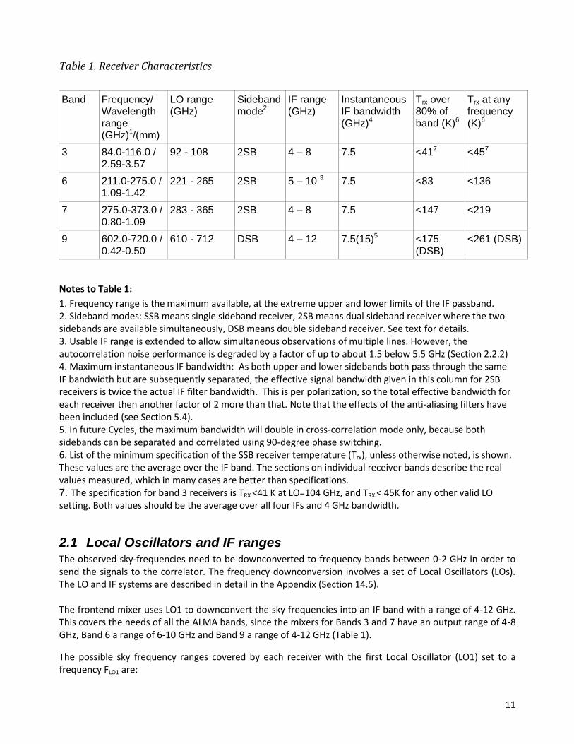
Table 1. Receiver Characteristics

Band Frequency/ Wavelength range (GHz)1/(mm)

LO range (GHz)

Sideband mode2

IF range (GHz)

Instantaneous IF bandwidth (GHz)4

Trx over 80% of band (K)6

Trx at any frequency (K)6

3 84.0-116.0 / 2.59-3.57

92 - 108 2SB 4 – 8 7.5 <417 <457

6 211.0-275.0 / 1.09-1.42

221 - 265 2SB 5 – 10 3 7.5 <83 <136

7 275.0-373.0 / 0.80-1.09

283 - 365 2SB 4 – 8 7.5 <147 <219

9 602.0-720.0 / 0.42-0.50

610 - 712 DSB 4 – 12 7.5(15)5 <175 (DSB)

<261 (DSB)

Notes to Table 1:

1. Frequency range is the maximum available, at the extreme upper and lower limits of the IF passband. 2. Sideband modes: SSB means single sideband receiver, 2SB means dual sideband receiver where the two sidebands are available simultaneously, DSB means double sideband receiver. See text for details. 3. Usable IF range is extended to allow simultaneous observations of multiple lines. However, the autocorrelation noise performance is degraded by a factor of up to about 1.5 below 5.5 GHz (Section 2.2.2) 4. Maximum instantaneous IF bandwidth: As both upper and lower sidebands both pass through the same IF bandwidth but are subsequently separated, the effective signal bandwidth given in this column for 2SB receivers is twice the actual IF filter bandwidth. This is per polarization, so the total effective bandwidth for each receiver then another factor of 2 more than that. Note that the effects of the anti-aliasing filters have been included (see Section 5.4). 5. In future Cycles, the maximum bandwidth will double in cross-correlation mode only, because both sidebands can be separated and correlated using 90-degree phase switching. 6. List of the minimum specification of the SSB receiver temperature (Trx), unless otherwise noted, is shown. These values are the average over the IF band. The sections on individual receiver bands describe the real values measured, which in many cases are better than specifications. 7. The specification for band 3 receivers is TRX <41 K at LO=104 GHz, and TRX < 45K for any other valid LO setting. Both values should be the average over all four IFs and 4 GHz bandwidth.

2.1 Local Oscillators and IF ranges The observed sky-frequencies need to be downconverted to frequency bands between 0-2 GHz in order to send the signals to the correlator. The frequency downconversion involves a set of Local Oscillators (LOs). The LO and IF systems are described in detail in the Appendix (Section 14.5). The frontend mixer uses LO1 to downconvert the sky frequencies into an IF band with a range of 4-12 GHz. This covers the needs of all the ALMA bands, since the mixers for Bands 3 and 7 have an output range of 4-8 GHz, Band 6 a range of 6-10 GHz and Band 9 a range of 4-12 GHz (Table 1).

The possible sky frequency ranges covered by each receiver with the first Local Oscillator (LO1) set to a frequency FLO1 are:

12

for the lower sideband (LSB): (FLO1 – IFlo) to (FLO1 – IFhi) for the upper sideband (USB): (FLO1 + IFlo) to (FLO1 + IFhi) where IFlo and IFhi are the lower and upper IF ranges in the “IF Range” column of Table 1, and the IF bandwidth (per sideband) is IFhi- IFlo.. This is illustrated in Figure 2. Note that the maximum IF bandwidth in Table 1 may be a few percent less than the IF range (see Section 5.4).

Figure 2. IF ranges for the two sidebands in a heterodyne receiver.

2.2 The Cycle 0 Receivers The Band 3, 6 and 7 receivers are dual-sideband (2SB) receivers, where both the upper and lower sidebands are provided separately and simultaneously. There are 4 outputs from each of the receivers, comprising the upper and lower sidebands in each of the two polarizations. Each output has a bandwidth of 4 GHz (reduced to an effective total bandwidth of 3.75 GHz due to the anti-aliasing filters, etc, see Section 5.4. The mixers give 10 dB or more unwanted sideband rejection, which is adequate for reducing the degradation of S/N from noise in the unwanted sideband, but not adequate for suppressing astronomical signals in the unwanted sideband. Further suppression is performed by offsetting LO1 and LO2 (and eventually the tunable filter LO, TFB LO) by small and opposite amounts, which depend on the antenna, such that the signals from two antennas in the image sideband do not correlate. The Band 9 receivers are double-sideband (DSB) receivers, where the IF contains noise and signals from both sidebands. They only have two outputs, one per polarization. However, the IF effective bandwidth is 7.5 GHz per sideband (after passing through the IF processing units), so the total instantaneous bandwidth is the same as Bands 3, 6 and 7. In Cycle 0, only one sideband per spectral window will be correlated, and the other rejected using LO offsetting, as mentioned above. This does not remove the noise from the rejected sideband. The noise of the sideband that is kept will be twice that of the DSB noise level. In the future, suitable phase switching will be introduced in the correlator, and both sidebands can be correlated and processed independently, thus doubling the effective system bandwidth. Each of the ALMA receiver bands is different in several aspects, and the following sections describe the individual receiver bands in more detail.

13

2.2.1 Band 3 receiver

Band 3 is the lowest frequency band available in Cycle 0, covering a frequency range of 84.0-116.0 GHz (the 3 mm atmospheric window). The cartridge is fed by a “periscope“ pair of ellipsoidal pickoff mirrors located outside the cryostat, which refocus the beam through the cryostat window, allowing for a smaller window diameter (Figure 3). A single feedhorn feeds an ortho-mode-transducer (OMT) which splits the two linear polarizations and feeds the SIS mixers.

Figure 3. Input optics for Band 3, showing the warm pickoff mirrors. The location of the antenna beam from the secondary mirror is shown by the dashed line, and the Cassegrain focus is shown by the small circle to the upper right. A new version of this Figure is being prepared by the FE group.

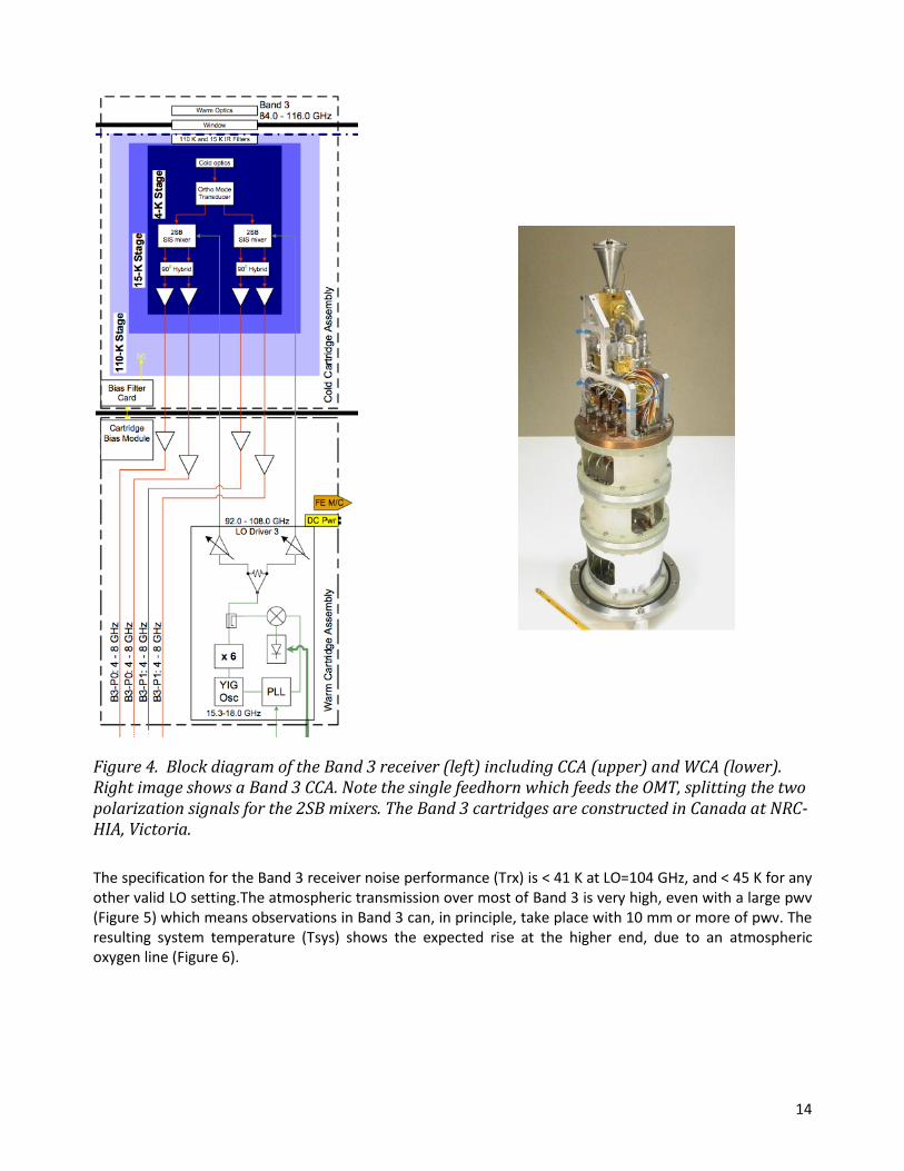
A block diagram of the Band 3 receiver, including the cold cartridge and warm cartridge assembly, is shown in Figure 4. The Cold Cartridge Assembly (CCA) contains the cold optics, OMT, SIS mixers and the low-noise HEMT first IF amplifiers. At room temperature, the Warm Cartridge Assembly (WCA) includes further IF amplification and the Local Oscillator covering 92-108 GHz.

14

Figure 4. Block diagram of the Band 3 receiver (left) including CCA (upper) and WCA (lower). Right image shows a Band 3 CCA. Note the single feedhorn which feeds the OMT, splitting the two polarization signals for the 2SB mixers. The Band 3 cartridges are constructed in Canada at NRC-HIA, Victoria.

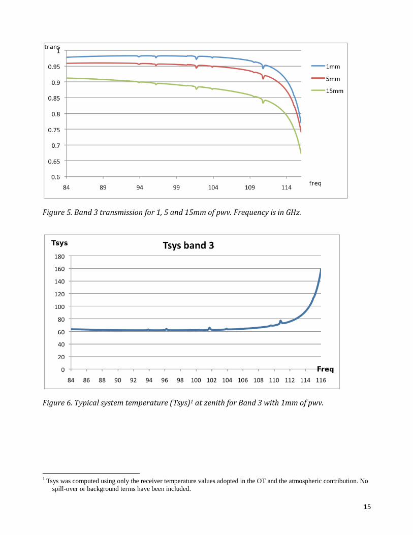
The specification for the Band 3 receiver noise performance (Trx) is < 41 K at LO=104 GHz, and < 45 K for any other valid LO setting.The atmospheric transmission over most of Band 3 is very high, even with a large pwv (Figure 5) which means observations in Band 3 can, in principle, take place with 10 mm or more of pwv. The resulting system temperature (Tsys) shows the expected rise at the higher end, due to an atmospheric oxygen line (Figure 6).

15

Figure 5. Band 3 transmission for 1, 5 and 15mm of pwv. Frequency is in GHz.

Figure 6. Typical system temperature (Tsys)1 at zenith for Band 3 with 1mm of pwv.

1 Tsys was computed using only the receiver temperature values adopted in the OT and the atmospheric contribution. No

spill-over or background terms have been included.

16


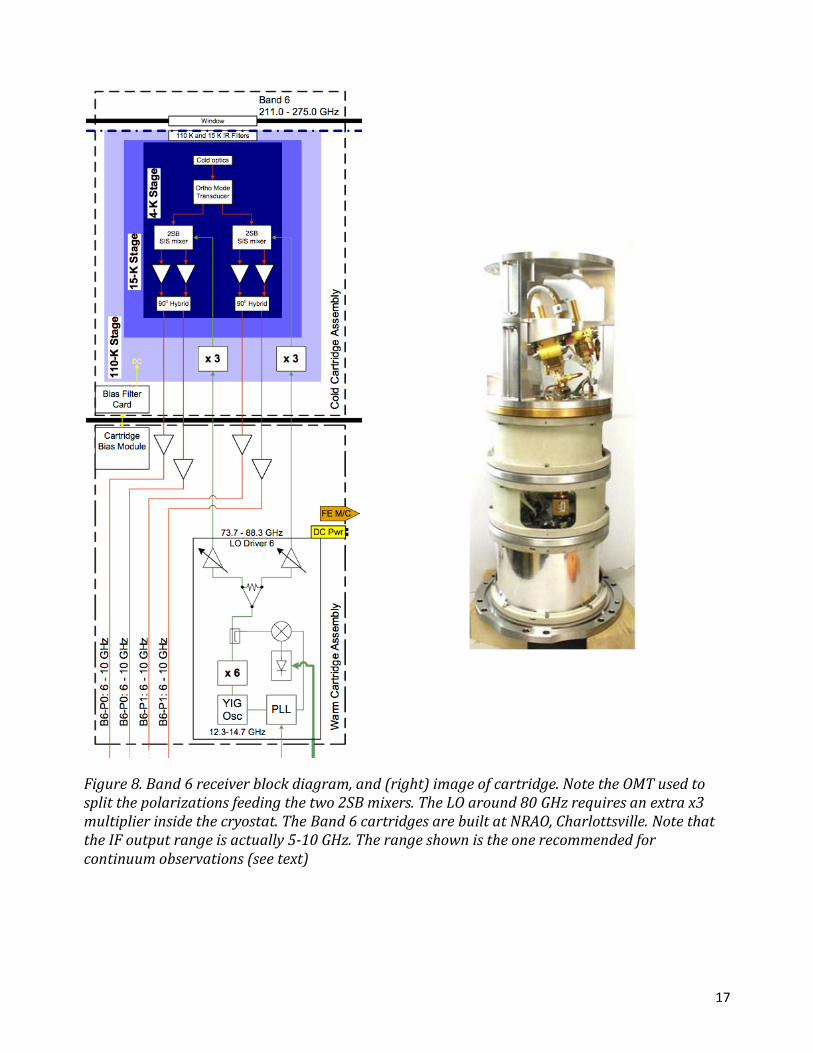
The Band 6 receiver covers a frequency range of 211.0-275.0 GHz (the 1.3 mm atmospheric window). This receiver has a window with a pair of off-axis ellipsoidal mirrors inside the cryostat (Figure 7). A single feedhorn feeds an ortho-mode-transducer (OMT) which splits the two linear polarizations and feeds the SIS mixers. A block diagram of the Band 6 receiver, including the cold cartridge and warm cartridge assembly, is shown in Figure 8.

Figure 7. Band 6 cold off-axis ellipsoidal mirrors feeding the single feedhorn. The off-axis beam from the telescope secondary mirror (shown by the dashed line) feeds directly through the cryostat window, and the Cassegrain focus is just inside the inner infrared blocker. Note the slightly inclined inner window, designed to minimize standing waves.

17

Figure 8. Band 6 receiver block diagram, and (right) image of cartridge. Note the OMT used to split the polarizations feeding the two 2SB mixers. The LO around 80 GHz requires an extra x3 multiplier inside the cryostat. The Band 6 cartridges are built at NRAO, Charlottsville. Note that the IF output range is actually 5-10 GHz. The range shown is the one recommended for continuum observations (see text)

18

The Band 6 IF frequency was recently extended to allow for multiple simultaneous line observations2; it now covers the range 5.0-10.0 GHz. There is 10-50 % excess noise below 5.5 GHz due to the LO1. It is therefore recommended that for continuum observations, the range 6-10 GHz is used. Also, it should be noted that the full range 5-10 GHz cannot be completely sampled because of the width of the two basebands per polarization. The atmospheric transmission in Band 6 is shown in Figure 9 for three typical pwv values. Most of the narrow absorption lines are from ozone. Most observations in Band 6 will be done with pwv < 5mm.

Figure 9. Band 6 zenith transmission for pwv=0.5, 1 and 5mm. Frequency is in GHz.

The specification for Band 6 receiver noise performance (Trx) is < 83 K over 80% of the band, and < 138 K over the whole band (SSB Trx). The measured results are considerably better, typically 50 K over most of the band. The resulting system temperatures (Tsys) for 1mm pwv are shown in Figure 10.

2 Specifically, the 12CO/13CO/C18O J=2-1 combination at 230.538/220.398/219.560 GHz, which has a minimum

separation of 10.14 GHz and requires the IF to reach to 5.0 GHz in order to cover all three lines

19

Figure 10. Typical Tsys3 at zenith for Band 6 with 1mm pwv, based on measured values of the receiver temperatures.



20


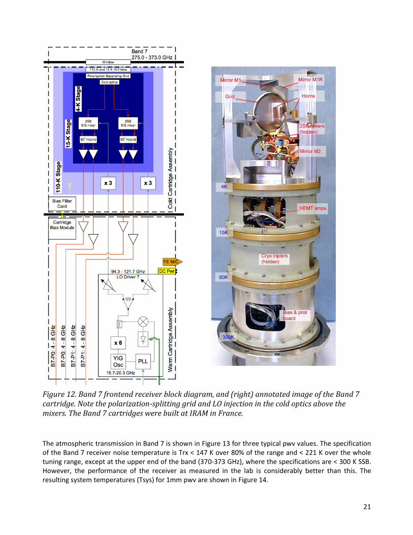
The Band 7 receiver covers the frequency range 275 - 373 GHz (the 0.85 mm atmospheric window). It has a

similar cold optics design as Band 6, but uses a wire-grid polarization splitter instead of an OMT, because the

losses in the OMT are higher at these frequencies (Figure 11). A block diagram of the Band 7 receiver,

including the cold cartridge and warm cartridge assembly, is shown in Figure 12.

Figure 11. Band 7 cold optics arrangement, showing the off-axis ellipsoidal mirrors and the polarization splitter wire grid.

21

Figure 12. Band 7 frontend receiver block diagram, and (right) annotated image of the Band 7 cartridge. Note the polarization-splitting grid and LO injection in the cold optics above the mixers. The Band 7 cartridges were built at IRAM in France.

The atmospheric transmission in Band 7 is shown in Figure 13 for three typical pwv values. The specification of the Band 7 receiver noise temperature is Trx < 147 K over 80% of the range and < 221 K over the whole tuning range, except at the upper end of the band (370-373 GHz), where the specifications are < 300 K SSB. However, the performance of the receiver as measured in the lab is considerably better than this. The resulting system temperatures (Tsys) for 1mm pwv are shown in Figure 14.

22

.

Figure 13. Band 7 atmospheric zenith transmission for pwv=0.5, 1.0 and 5.0mm. Frequency is in GHz.

Figure 14. Typical Tsys4 at zenith for Band 7 with pwv=1mm.



23


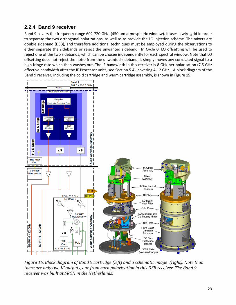
Band 9 covers the frequency range 602-720 GHz (450 um atmospheric window). It uses a wire grid in order to separate the two orthogonal polarizations, as well as to provide the LO injection scheme. The mixers are double sideband (DSB), and therefore additional techniques must be employed during the observations to either separate the sidebands or reject the unwanted sideband. In Cycle 0, LO offsetting will be used to reject one of the two sidebands, which can be chosen independently for each spectral window. Note that LO offsetting does not reject the noise from the unwanted sideband, it simply moves any correlated signal to a high fringe rate which then washes out. The IF bandwidth in this receiver is 8 GHz per polarisation (7.5 GHz effective bandwidth after the IF Processor units, see Section 5.4), covering 4-12 GHz. A block diagram of the Band 9 receiver, including the cold cartridge and warm cartridge assembly, is shown in Figure 15.

Figure 15. Block diagram of Band 9 cartridge (left) and a schematic image (right). Note that there are only two IF outputs, one from each polarization in this DSB receiver. The Band 9 receiver was built at SRON in the Netherlands.

24

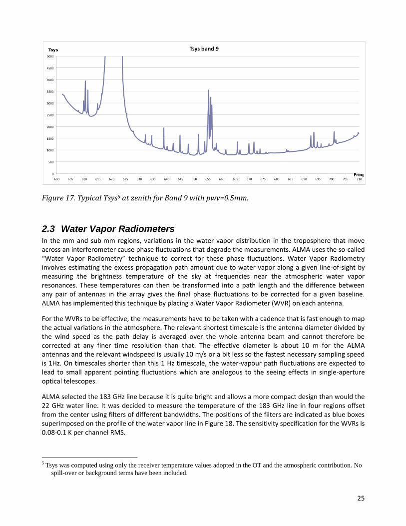
The Band 9 atmospheric transmission is significantly dependent on the pwv, as illustrated in Figure 16 for 3 low values of pwv. The specifications for the receiver are Trx < 175 K over 80% of the band and < 261 K over all the band. However, the performance is considerably better than this, and Figure 17 shows the expected Tsys for 0.5 mm of pwv, over most of the band given the expected receiver noise. As well as having a lower atmospheric transmission and a less stable atmosphere, Band 9 observing provides several challenges for observing: finding sufficiently bright calibrators (most QSOs are relatively faint at this frequency), requiring accurate pointing for the relatively small primary beam, and the need for the highest level of stability in the rest of the system.

Figure 16. Band 9 zenith transmission for pwv = 0.2, 0.5 and 1mm. Frequency is in GHz.

25

Figure 17. Typical Tsys5 at zenith for Band 9 with pwv=0.5mm.

2.3 Water Vapor Radiometers In the mm and sub-mm regions, variations in the water vapor distribution in the troposphere that move across an interferometer cause phase fluctuations that degrade the measurements. ALMA uses the so-called “Water Vapor Radiometry” technique to correct for these phase fluctuations. Water Vapor Radiometry involves estimating the excess propagation path amount due to water vapor along a given line-of-sight by measuring the brightness temperature of the sky at frequencies near the atmospheric water vapor resonances. These temperatures can then be transformed into a path length and the difference between any pair of antennas in the array gives the final phase fluctuations to be corrected for a given baseline. ALMA has implemented this technique by placing a Water Vapor Radiometer (WVR) on each antenna.

For the WVRs to be effective, the measurements have to be taken with a cadence that is fast enough to map the actual variations in the atmosphere. The relevant shortest timescale is the antenna diameter divided by the wind speed as the path delay is averaged over the whole antenna beam and cannot therefore be corrected at any finer time resolution than that. The effective diameter is about 10 m for the ALMA antennas and the relevant windspeed is usually 10 m/s or a bit less so the fastest necessary sampling speed is 1Hz. On timescales shorter than this 1 Hz timescale, the water-vapour path fluctuations are expected to lead to small apparent pointing fluctuations which are analogous to the seeing effects in single-aperture optical telescopes.

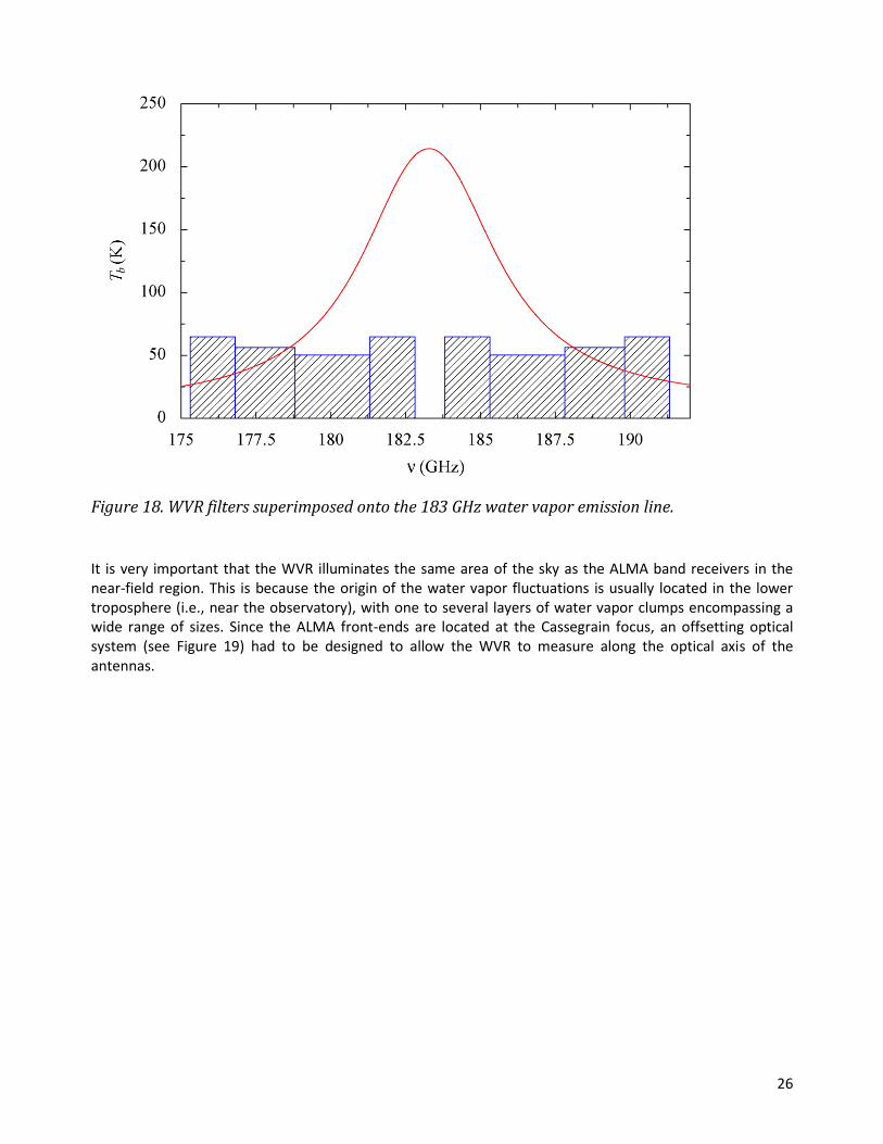
ALMA selected the 183 GHz line because it is quite bright and allows a more compact design than would the 22 GHz water line. It was decided to measure the temperature of the 183 GHz line in four regions offset from the center using filters of different bandwidths. The positions of the filters are indicated as blue boxes superimposed on the profile of the water vapor line in Figure 18. The sensitivity specification for the WVRs is 0.08-0.1 K per channel RMS.



26

Figure 18. WVR filters superimposed onto the 183 GHz water vapor emission line.

It is very important that the WVR illuminates the same area of the sky as the ALMA band receivers in the near-field region. This is because the origin of the water vapor fluctuations is usually located in the lower troposphere (i.e., near the observatory), with one to several layers of water vapor clumps encompassing a wide range of sizes. Since the ALMA front-ends are located at the Cassegrain focus, an offsetting optical system (see Figure 19) had to be designed to allow the WVR to measure along the optical axis of the antennas.

27

Figure 19. Offset optics used to collect the sky emission along the optical axis of the antenna into the WVR.

The WVRs are only able to detect the variations in atmospheric brightness temperatures due to the “wet” atmosphere (i.e., pwv). There are also variations due to the changes in bulk ambient temperature at different heights above the observatory. It is expected that these could become significant during day time and some techniques are being currently studied to try to measure them (including thermal sounders of the atmosphere that use the profiles of the emission of the oxygen molecules).

The brightness temperature variations of the sky that the WVRs have to detect are sometimes quite small, so the quality of the receiving system becomes very important. In fact, the current specification for the ALMA WVRs is that they need to allow corrections of the path fluctuations (in μm):

where w is the total water vapor content along the line of sight, and Lraw the total fluctuations observed at any given time. Therefore, this formula includes the expected error of about 2% in measuring the total fluctuations, and states the total resulting path errors after correction (Lcorr). For a 1mm pwv, the residual term in the formula would be 20µm.

The stability specification for the WVRs is very stringent (0.1 K peak-to-peak over 10 minutes and 10 degree tilts). To achieve this, a Dicke-switching-radiometer approach was adopted. The input into the mixer is switched periodically (5.35 Hz) between two calibrated loads (the “cold” and “hot” loads at 293 K and 351 K, respectively), and the sky using a rotating vane embedded in the light path as shown in Figure 20.

28

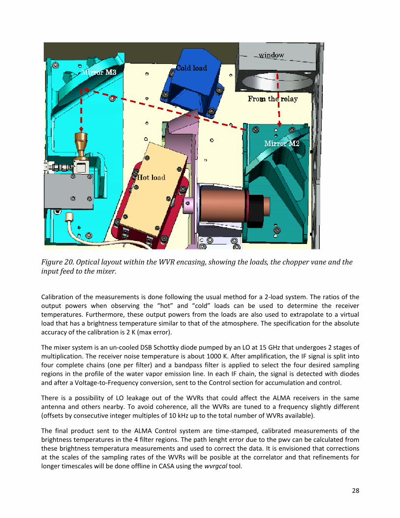
Figure 20. Optical layout within the WVR encasing, showing the loads, the chopper vane and the input feed to the mixer.

Calibration of the measurements is done following the usual method for a 2-load system. The ratios of the output powers when observing the “hot” and “cold” loads can be used to determine the receiver temperatures. Furthermore, these output powers from the loads are also used to extrapolate to a virtual load that has a brightness temperature similar to that of the atmosphere. The specification for the absolute accuracy of the calibration is 2 K (max error).

The mixer system is an un-cooled DSB Schottky diode pumped by an LO at 15 GHz that undergoes 2 stages of multiplication. The receiver noise temperature is about 1000 K. After amplification, the IF signal is split into four complete chains (one per filter) and a bandpass filter is applied to select the four desired sampling regions in the profile of the water vapor emission line. In each IF chain, the signal is detected with diodes and after a Voltage-to-Frequency conversion, sent to the Control section for accumulation and control.

There is a possibility of LO leakage out of the WVRs that could affect the ALMA receivers in the same antenna and others nearby. To avoid coherence, all the WVRs are tuned to a frequency slightly different (offsets by consecutive integer multiples of 10 kHz up to the total number of WVRs available).

The final product sent to the ALMA Control system are time-stamped, calibrated measurements of the brightness temperatures in the 4 filter regions. The path lenght error due to the pwv can be calculated from these brightness temperatura measurements and used to correct the data. It is envisioned that corrections at the scales of the sampling rates of the WVRs will be posible at the correlator and that refinements for longer timescales will be done offline in CASA using the wvrgcal tool.

29

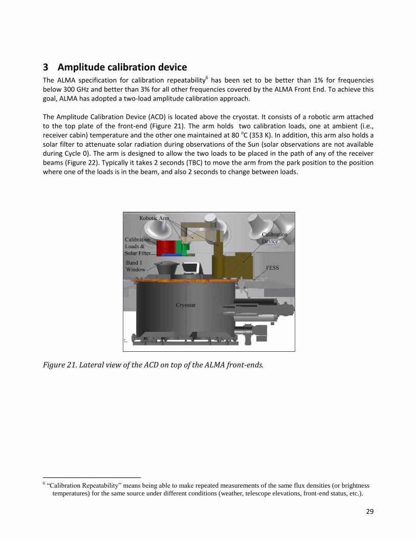
3 Amplitude calibration device The ALMA specification for calibration repeatability6 has been set to be better than 1% for frequencies below 300 GHz and better than 3% for all other frequencies covered by the ALMA Front End. To achieve this goal, ALMA has adopted a two-load amplitude calibration approach. The Amplitude Calibration Device (ACD) is located above the cryostat. It consists of a robotic arm attached to the top plate of the front-end (Figure 21). The arm holds two calibration loads, one at ambient (i.e., receiver cabin) temperature and the other one maintained at 80 oC (353 K). In addition, this arm also holds a solar filter to attenuate solar radiation during observations of the Sun (solar observations are not available during Cycle 0). The arm is designed to allow the two loads to be placed in the path of any of the receiver beams (Figure 22). Typically it takes 2 seconds (TBC) to move the arm from the park position to the position where one of the loads is in the beam, and also 2 seconds to change between loads.

Figure 21. Lateral view of the ACD on top of the ALMA front-ends.

6 “Calibration Repeatability” means being able to make repeated measurements of the same flux densities (or brightness

temperatures) for the same source under different conditions (weather, telescope elevations, front-end status, etc.).

30

Figure 22. Top view of an ALMA front end showing the robotic arm of the ACD retracted during normal observations or on top of one of the front-end inserts for calibration. The current design has been improved by placing all the loads in a wheel.

To accurately calibrate radio astronomical data to a temperature scale, the actual brightness of the two loads has to be precisely known. Critical to this calibration precision is the coupling of the load to the beam of a given band. This coupling must be very good at any telescope elevation and free of reflections of the load emission. This is because any reflection from the loads back into the cryostat would be terminated at a different temperature and would cause standing waves. Both loads have thus been designed so that the actual effective brightness temperature and that computed from the measured physical temperature (with sensors embedded in the loads) using known emissivities differ by, at most, +/- 0.3 K and +/- 1.0 K for the “ambient” and “hot” loads, respectively. This requirement also sets a limit to the fluctuations and departure from the set temperature that are allowed for the “hot” load. Furthermore, the return loss specifications for these loads are -60 dB and -56 dB, respectively.

3.1 Atmospheric Calibration Procedure The ACD is used to measure the receiver temperature and the sky emission by comparing the signals on the sky, ambient and hot loads. This is known as atmospheric calibration (ATM calibration), and is required to correct for differences in the atmospheric transmission between the science and the celestial amplitude calibrators. Normally ATM calibration is done during observations, both near the science target, as well as near the amplitude calibrator. Traditionally, most mm and sub-mm observatories have used the single-load calibration method, but several simulations have shown single-load calibration is not capable of reaching the calibration accuracies required by ALMA at all of its observing frequencies. However, that method has the very desirable feature that it is only weakly dependent on the opacity of the sky at the time of the observations.

A method, using the two calibration loads within the ACD, has been devised in the past to try to achieve the same weak dependence on the opacities at the time of the observation. This method (“the α method”) uses the voltage outputs from the observations of both loads to simulate a single load with a brightness temperature close to that of the atmosphere at the observing frequency. This fictitious single load is defined

31

as a weighted sum of the voltages of the “hot” and “ambient” loads so that the temperature calibration factors are almost independent of the optical depth.

The fictitious load voltage output, VL, is defined as:

21 )1( LLL VVV

where α is the weighting factor, and VL1, VL2 the output voltages when the two loads are measured. From this definition and some algebra, one can find the optimum weighting factor needed to minimize opacity dependency, and the corresponding resulting calibration factors are:

)()(

)1(

21

2

BGiMiBGsMsCAL

LL

LSPM

JJgeJJT

JJ

JJJ

is

where η is the forward efficiency of the antenna, g the sideband ratio, τ the opacity, and JM, JSP, JL1, JL2 and JBG are the emissivity temperatures of the average sky, the spill-over, the two loads and the background radiation, respectively. The subscripts s and i represent the signal and image bands, respectively. The system temperature is then derived using the formula:

SKYL

SKYCALsys

VV

VTT

For ALMA it has been found that with the current system, the non-linearities are the dominant source of error for this calibration. The system electronics and SIS mixers are not fully linear and dominate the calibration accuracy that can be achieved for Cycle 0.

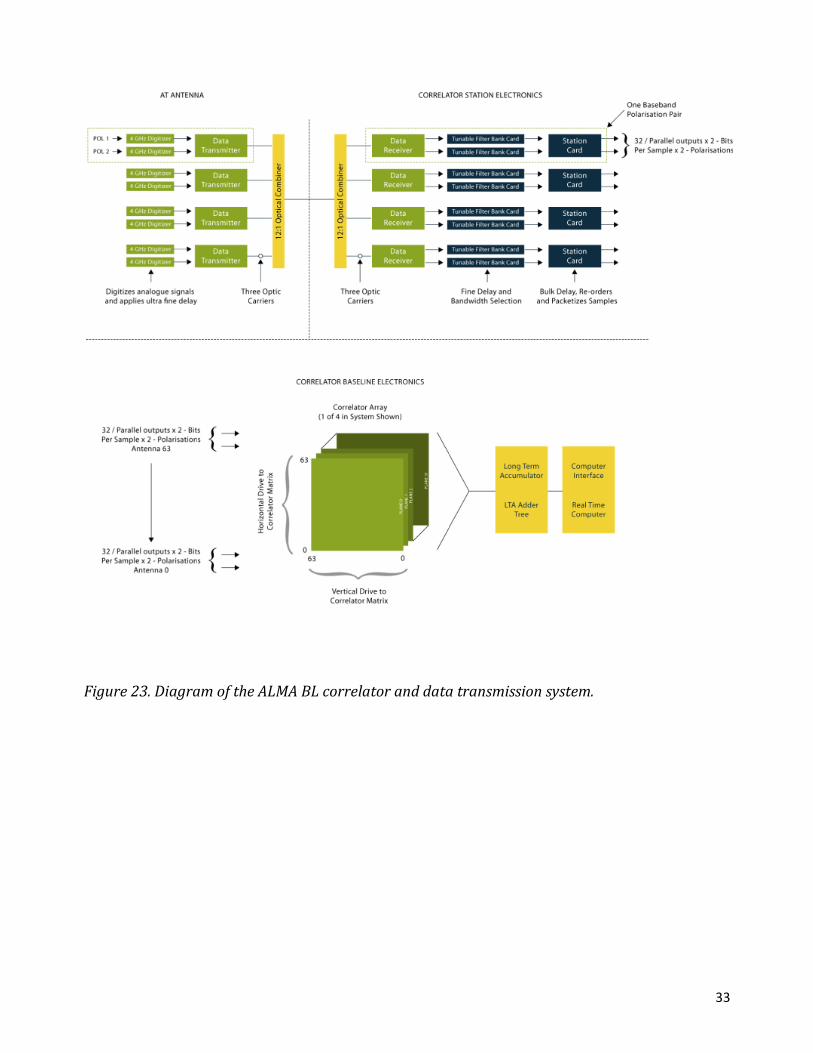
4 The Correlator As mentioned earlier the observed sky-frequencies need to be downconverted to frequency bands between 0-2 GHz in order to send the signals to the correlator. The frequency downconversion involves a set of Local Oscillators (LOs). The LO and IF systems are described in detail in the Appendix (Section 14.5). The frequency bands between 0-2 GHz are called basebands. The Correlator can handle up to 8 basebands simultaneously (4 basebands per polarization). The Correlator used in Cycle 0 (the 64-input Correlator) is of a digital hybrid design that enhances the performance of more traditional lag correlators (XF)7 called an FXF system. This correlator is described in detail in Escoffier et al. (2007, A&A 462, 801). It operates in two basic modes, TDM (Time Division Mode) for low resolution wideband continuum observations, and FDM (Frequency Division Mode) for higher spectral resolution modes that can be selectively sampled with “windows” or “sub-bands” within the baseband. The Correlator is physically located in the AOS Technical Building.

A simplified block diagram of the Correlator is shown in Figure 23. It consists of 4 quadrants. Each quadrant can handle a full baseband pair (defined as one of the basebands in each polarization) for up to 64 antennas for a total bandwidth per antenna of up to 16 GHz. The data is corrected for geometrical delays prior to processing, and for quantization errors during the processing. Two of the quadrants are available for Cycle 0.

7 X=correlation and F=Fourier Transform

32

They will be able to handle all baseband pairs for 32 antennas for a total bandwidth per antenna of up to 16 GHz (in 2 polarisations, that is 8 GHz per polarization).

In FDM mode each 2 GHz baseband is subdivided into as many as 32 sub-bands of 62.5 MHz bandwidth each. This is done using digital filtering in the Tunable Filterbanks (TFBs). To provide more than 62.5 MHz of bandwidth, multiple TFBs are set up for adjacent frequencies. To avoid aliasing and edge effects, only 15/16 of the total bandwidth from each TFB is used, giving a bandwidth per sub-band when operating in this mode of 58.5975 MHz (also the sub-band separation is 58.5975 MHz). The remaining edge channels are truncated within the correlator, and not visible in the data in FDM mode. The center frequency of each of the sub-bands will eventually be independently tunable for flexibility, but for Cycle 0 all TFBs in use are joined together in the data processing to give Spectral Windows (SPW) with nominal bandwidths from 62.5 to 2000.0 MHz in steps of 2, depending on the number of sub-bands used (but note the available bandwidth is 15/16 of these for reasons given above). At the output of the TFBs, the signals are re-quantized to 2 or 4 bits (for Cycle 0, only the 2-bit mode will be available, see Section 4.4) for correlation. FDM provides up to 7680 channels per baseband pair in Cycle 0. For N polarisation products, the number of channels is 7680/N. FDM is used mostly (although not exclusively) for spectral line observing. In TDM mode, the TFBs are bypassed and the full 2 GHz baseband is fed through the correlator. The signal is distributed in time over several correlator chips, each of which performs the cross-correlation for some fraction of the time. The correlations are then re-combined to get the fully time-sampled data. The TDM mode provides for up to 256 channels per baseband (for N polarisation products, the number of channels are reduced to 256/N), and no edge channels are dropped (the full 2000 MHz are covered, requiring some truncation of the edge channels in offline data processing – see Section 5.4). All the spectral channels are delivered in the datasets, but it is recommended that 1/16th of the baseband (i.e, 4 or 8 channels at each end of the spectrum for double and single polarization, respectively) is removed during the offline reduction. TDM is used mostly (although not exclusively) for continuum observing. TDM has the advantage of having a lower data rate and is therefore used for continuum pointing, focussing etc. In the cross-correlation modules, the multiply-and-add operations are performed at a clock rate of 125 MHz (4 GHz samples divided by 32). Each board (Figure 24) contains 64 4-k lag correlator chips, connected in a matrix to provide the required complex correlations. Cross-correlation data goes then to a time integrator (the Long Term Accumulator, LTA – Figure 23) that adds the data up to an integer multiple of 16 ms for cross-correlations and multiples of 1 ms for auto-correlations. The Fourier transforms are done on each sub-band and the final spectrum is formed by stitching together the sub-bands. There is a maximum number of spectral bins of 7680 per baseband in single polarisation, and 3840 in dual polarisation. The data can be further co-added in the Correlator Data Processor (CDP). It is expected that the CDP also will be used for real-time corrections of the phase fluctuations using the WVR data, although it is also possible to do this correction offline in CASA. Each baseband signal is fed to one correlator section, which can have several different bandwidth modes, although in Cycle 0, all the correlators need to be set to the same mode. The next section describes the further processing of the data from the correlator. The full list of correlator modes is given in the Capabilities page in the Science Portal: (http://www.almascience.org/call-for-proposals/capabilities).

33

Figure 23. Diagram of the ALMA BL correlator and data transmission system.

34

Figure 24. Correlator board, with the 8x8 array of custom correlator chips, each with 4k lags. There are 128 such boards per correlator quadrant adding up to a grand total of 32768 chips.

4.1 Correlator data processing – spectral and channel-average The correlator produces two datasets, the complete spectral data, and the channel-averaged data. These are normally written to the archive from the CDP (the central correlator computer) at different rates. The primary purpose of the channel-averaged data is to provide a smaller dataset for the online processing software, which computes real-time pointing and focus corrections. It is stored in the ASDM (ALMA Science Data Model) dataset as a separate spectral window from the channelized data, but should not normally be used for science purposes. The continuum data for science observing will need to be constructed offline in CASA (Common Astronomy Software Applications) using the appropriate portions of the channelized data. The channelized data contains the requested number of channels for each requested polarization product.

The time intervals involved at this stage of the observing and data aquisition are (see also Figure 25):

Dump duration: The internal time period inside the correlator (16 ms for cross correlations and multiples of 1 ms for auto-correlations) over which data is accumulated before sending to the CDP. Data can be corrected for atmospheric phase fluctuations using the WVR correction once every dump in the CDP, or offline in CASA. During observations the dump time in FDM mode should be in multiples of 48 ms and in TDM mode 32 ms.

Channel average time: time interval between channel average data being sent to the archive. The channel average time must be a multiple of the dump duration.

Spectral integration time: Spectral data is sent from the correlator to the archive (and ASDM) once per spectral integration time. The spectral integration time must be a multiple of the dump duration. It is also usually set to be a multiple of the channel average time.

Subscan duration: total time per subscan. In an observation, this will effectively be the shortest time interval integrating on the source (or on a load, or in the raster scan in total power mode). The subscan duration must be a multiple of the spectral integration time.

Scan time: total time per scan. Must be a multiple of the subscan duration.

35

Figure 25. Data processing and accumulation steps in the correlator and archive. The timing intervals shown are described in the text.

4.1.1 Final data product – the ASDM

The final data product in the archive is the ASDM (the ALMA Scince Data Model). In the ASDM the bulk data are saved as two spectral windows, one (with a dimension of 1 channel per polarisation product) for the channel average and one (with a dimension of N channels per polarisation product) for the spectral data. In addition to the data from each spectral window, the WVR data is also stored as a series of four spectral windows near 183 GHz. The ASDM is described in more detail in Section 10.5.

4.2 Spectral resolution and smoothing

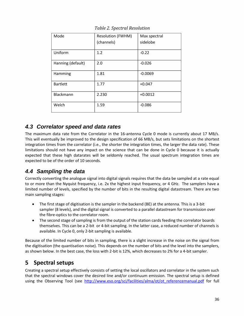
It is possible to select various spectral smoothing functions in the correlator (see Table 2). These provide different levels of smoothing and (spectral) sidelobe levels (see http://mathworld.wolfram.com/ApodizationFunction.html for a full description of these). The default is Hanning, which means that the spectral resolution of the data will be 2.0 x the channel spacing.

http://mathworld.wolfram.com/ApodizationFunction.html

36

Table 2. Spectral Resolution

Mode Resolution (FWHM)

(channels)

Max spectral

sidelobe

Uniform 1.2 -0.22

Hanning (default) 2.0 -0.026

Hamming 1.81 -0.0069

Bartlett 1.77 +0.047

Blackmann 2.230 +0.0012

Welch 1.59 -0.086

4.3 Correlator speed and data rates

The maximum data rate from the Correlator in the 16-antenna Cycle 0 mode is currently about 17 MB/s. This will eventually be improved to the design specification of 66 MB/s, but sets limitations on the shortest integration times from the correlator (i.e., the shorter the integration times, the larger the data rate). These limitations should not have any impact on the science that can be done in Cycle 0 because it is actually expected that these high datarates will be seldomly reached. The usual spectrum integration times are expected to be of the order of 10 seconds.

4.4 Sampling the data Correctly converting the analogue signal into digital signals requires that the data be sampled at a rate equal to or more than the Nyquist frequency, i.e. 2x the highest input frequency, or 4 GHz. The samplers have a limited number of levels, specified by the number of bits in the resulting digital datastream. There are two main sampling stages:

The first stage of digitisation is the sampler in the backend (BE) at the antenna. This is a 3-bit sampler (8 levels), and the digital signal is converted to a parallel datastream for transmission over the fibre-optics to the correlator room.

The second stage of sampling is from the output of the station cards feeding the correlator boards themselves. This can be a 2-bit or 4-bit sampling. In the latter case, a reduced number of channels is available. In Cycle 0, only 2-bit sampling is available.

Because of the limited number of bits in sampling, there is a slight increase in the noise on the signal from the digitisation (the quantisation noise). This depends on the number of bits and the level into the samplers, as shown below. In the best case, the loss with 2-bit is 12%, which decreases to 2% for a 4-bit sampler.

5 Spectral setups Creating a spectral setup effectively consists of setting the local oscillators and correlator in the system such that the spectral windows cover the desired line and/or continuum emission. The spectral setup is defined using the Observing Tool (see http://www.eso.org/sci/facilities/alma/ot/ot_referencemanual.pdf for full

http://www.eso.org/sci/facilities/alma/ot/ot_referencemanual.pdf

37

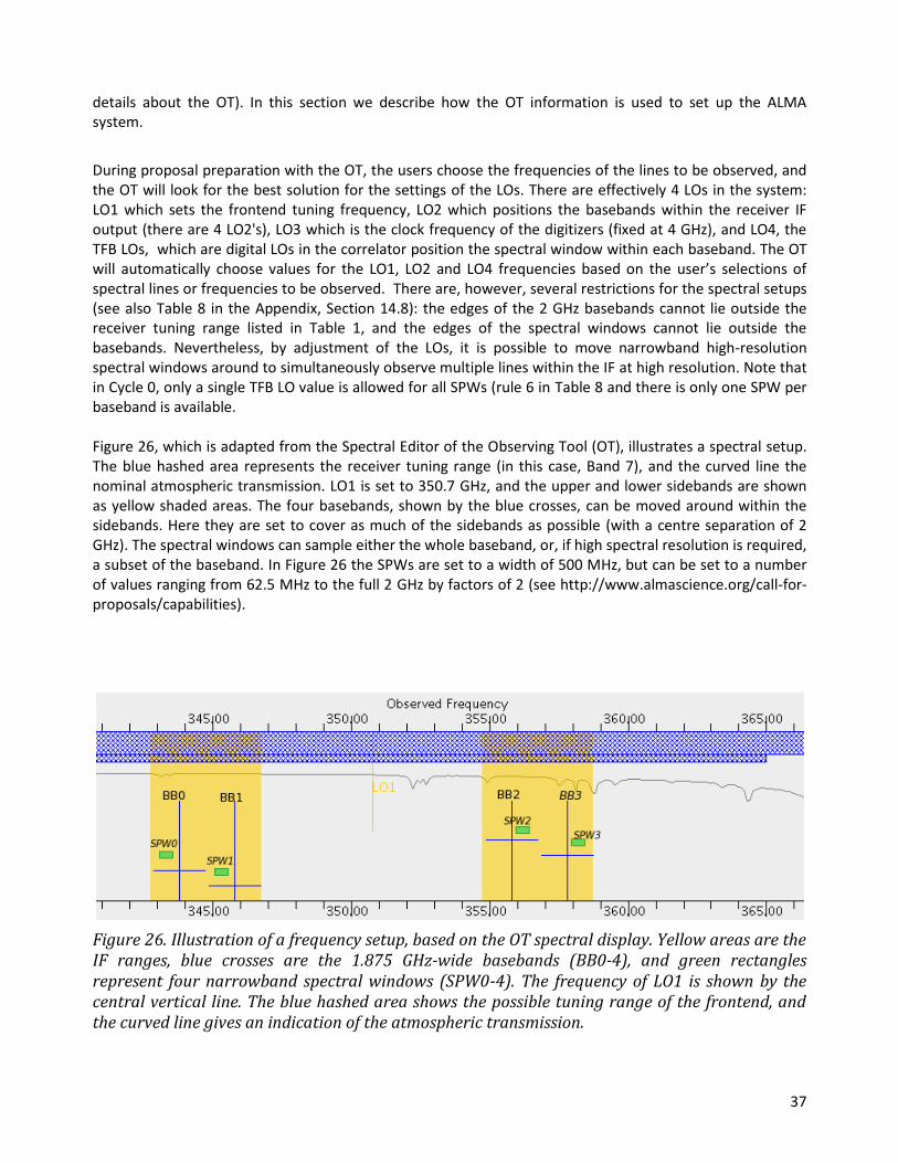
details about the OT). In this section we describe how the OT information is used to set up the ALMA system.

During proposal preparation with the OT, the users choose the frequencies of the lines to be observed, and the OT will look for the best solution for the settings of the LOs. There are effectively 4 LOs in the system: LO1 which sets the frontend tuning frequency, LO2 which positions the basebands within the receiver IF output (there are 4 LO2's), LO3 which is the clock frequency of the digitizers (fixed at 4 GHz), and LO4, the TFB LOs, which are digital LOs in the correlator position the spectral window within each baseband. The OT will automatically choose values for the LO1, LO2 and LO4 frequencies based on the user’s selections of spectral lines or frequencies to be observed. There are, however, several restrictions for the spectral setups (see also Table 8 in the Appendix, Section 14.8): the edges of the 2 GHz basebands cannot lie outside the receiver tuning range listed in Table 1, and the edges of the spectral windows cannot lie outside the basebands. Nevertheless, by adjustment of the LOs, it is possible to move narrowband high-resolution spectral windows around to simultaneously observe multiple lines within the IF at high resolution. Note that in Cycle 0, only a single TFB LO value is allowed for all SPWs (rule 6 in Table 8 and there is only one SPW per baseband is available. Figure 26, which is adapted from the Spectral Editor of the Observing Tool (OT), illustrates a spectral setup. The blue hashed area represents the receiver tuning range (in this case, Band 7), and the curved line the nominal atmospheric transmission. LO1 is set to 350.7 GHz, and the upper and lower sidebands are shown as yellow shaded areas. The four basebands, shown by the blue crosses, can be moved around within the sidebands. Here they are set to cover as much of the sidebands as possible (with a centre separation of 2 GHz). The spectral windows can sample either the whole baseband, or, if high spectral resolution is required, a subset of the baseband. In Figure 26 the SPWs are set to a width of 500 MHz, but can be set to a number of values ranging from 62.5 MHz to the full 2 GHz by factors of 2 (see http://www.almascience.org/call-for-proposals/capabilities).

Figure 26. Illustration of a frequency setup, based on the OT spectral display. Yellow areas are the IF ranges, blue crosses are the 1.875 GHz-wide basebands (BB0-4), and green rectangles represent four narrowband spectral windows (SPW0-4). The frequency of LO1 is shown by the central vertical line. The blue hashed area shows the possible tuning range of the frontend, and the curved line gives an indication of the atmospheric transmission.

38

5.1 Spectral setups for multiple lines The wide IF bandwidth and tuning ability allows for simultaneous imaging of multiple lines. However, the restrictions for Cycle 0 means that setting up spectral windows with multiple lines is more involved at this stage. Some template setups will be available within the OT. Some examples (with the approximate line frequencies in GHz) are shown in Table 3 (for a redshift of zero). Note that when only 3 basebands are listed, the fourth one would normally be set up for a continuum observation (or perhaps a fainter line). Also, except in some cases, the lines will not generally appear in the center of the SPWs.

Table 3. Examples of multiple bright line configurations possible in Cycle 0.

Band Species/transition Frequency Sideband bandwidth baseband

3 HCO+ 1-0 89.188 LSB 62.5 1

HCN 1-0 88.632 LSB 62.5 2

CH3OH 101.293 USB 62.5 3

H2CO 101.333 USB 62.5 3

6 12CO 2-1 230.538 USB 500 1

C18O 2-1 219.560 LSB 500 2 13CO 2-1 220.399 LSB 500 3

7 12CO 3-2 345.796 LSB 500 1

HCO+ 4-3 356.743 USB 500 2

HCN 4-3 354.505 USB 500 3

9 12CO 6-5 691.472 USB 500 1

CS 14-13 685.436 USB 500 2

H2S 687.303 USB 500 3

C17O 6-5 674.009 LSB 500 4

5.2 Spectral setups for lines near the edge of the bands The Cycle 0 version of the OT only allows lines to be observed at the centre of SPWs. There is also a restriction that the selected bandwidth cannot fall outside the maximum or minimum tuning range of the receiver. This is an issue for certain lines at the edge of the tuning range. One example is observations of the 12CO(J=1-0) line at a redshift of zero (at 115.271 GHz), which is close to the maximum tuning range of Band 3 (116 GHz, see Table 1). A setup using the 2 GHz mode will not validate within the OT. The solution is to set the observing frequency to a lower value, which offsets the line transition from the SPW centre. For example if the observing frequency is set to 115.000 GHz, the setup will validate and the line will still appear within the SPW.

5.3 Observing lines and continuum

Simultaneous observations of both line emission and continuum are possible. To maximise the continuum sensitivity, one of the widest bandwidth modes should be chosen (i.e. 1.875 GHz in FDM or 2 GHz in TDM; the usable bandwith in both cases will be 1.875 GHz – see Section 5.4). Note that in Cycle 0 it will not be possible to mix correlator modes, e.g. a spectral window with a bandwidth of 1.875 GHz and another with a width of 62.5 MHz. Therefore there may be a compromise required between the need of high spectral

39

resolution and maximising the total bandwidth and sensitivity for continuum. If this type of observation is required, an option is to select a mode with just enough resolution for the spectral line observations, which would yield the largest bandwidth for continuum. Another option is to set up two separate science goals (which will require more observing time).

5.4 Usable bandwidth The IF system contains an anti-aliasing filter which limits the bandwidth of the basebands. Nominally this filter has -1dB points at 2.10 and 3.90 GHz, giving a maximum bandwidth of 1.8 GHz. However, the IF response is such that the usable bandwidth is slightly higher – i.e., 1.875 GHz. In FDM mode, the correlator outputs a bandwidth of 1.875 GHz, thus in FDM, the full bandwidth in wideband mode can be used. In TDM the correlator outputs a bandwidth of 2.000 GHz, but typically the edges of the spectra are affected by low power due to this filter and some ringing effects. It is recommended that 4 (double polarization) or 8 (single polarization) channels are filtered manually offline. This results in the same usable bandwidth in both TDM and FDM modes and is illustrated in Figure 27.

Figure 27. Comparison of TDM (left) and FDM (right) showing the dropoff in total power at the edges in the two modes. Colours represent the two polarisations from an example antenna. The 2.0 GHz bandwidth output from the correlator in TDM mode shows the drop in power in the upper and lower ~4 channels due to the anti-aliasing filter. In FDM, only the central 1.875 GHz is output from the correlator, and the drop in power at the edges of this bandwidth is negligible.

6 Cycle 0 Configurations

6.1 Introduction The basic data produced by ALMA are the visibilities which sample the sky emission of the field of view in the Fourier plane. These visibilities are obtained by the correlation of the signal for each pair of antennas. Thus, the location of the antennas constrain the angular resolution, the dynamic range and the reliability of the reconstructed images. ALMA will have in total 192 antenna pads for the 66 antennas. During Cycle 0 the 16 antennas will be placed on a smaller set of pads located in the the central part of the array. Cycle 0 will

40

include two different array configurations in order to achieve different angular resolutions and to get a reasonable coverage of short baselines for imaging of extended sources. The antennas will be moved from one configuration to the other according to Section 3 in the Capabilities section of the ALMA Science Portal: http://almascience.org/call-for-proposals/capabilities, and science projects will be observed in the configuration best suited for the requested spatial resolution, and, more generally, the uv-coverage.

The angular resolution achievable during a given observation depends on the uv-coverage and the inversion process from the uv-plane to the real image. However, it has been found that a good measure of it is obtained by using the RMS projected baseline (BRMS) of the observations. A rule-of-thumb would thus be:

Moreover the Field of View (FOV) of an observation is given by the size of the primary beam of the antenna with a diameter D (in meter) at a frequency f (in GHz). Using the Half Power Beam Width as an estimate, the FOV is given by:

Finally, a rule-of-thumb used to define the maximum angular scales observable by an interferometer is 0.6

times the ratio of the wavelength to the minimum baseline (Bmin) projected in the direction of the source

(hereafter the Maximum Scale). This corresponds to structures whose flux would be recovered only at the

10 % level. Angular scales larger that these are still detectable, but very little flux would be recovered from

them (i.e., the structures are “resolved out”). It should be noted that this applies to extended structures in

both of any pair of orthogonal directions on the sky. Following the preceding nomenclature:

For Cycle 0 the number of antennas/baselines available is still not enough to give a very good snapshot performance. This implies that for sources that are not point-like, some uv-information may be missed with short observations. This affects the imaging performance of the observations, especially if the sources are highly asymmetric and/or whenever a high imaging dynamic range is desired (> 100). For the cases outlined above (and whenever the source shape is NOT well-known, just the extent), observations of the same source covering a range of Hour Angles are advisable and should be explicitly requested by the PIs.

6.2 The Two Cycle 0 Configurations

6.2.1 The Cycle 0 Compact Configuration

The Compact configuration aims to provide good uv-coverage for extended sources with a lower angular resolution than the Extended configuration (see Table 4 and 5). It is designed to give good uv coverage of extended sources and therefore an excess, with respect to a pure Gaussian distribution, of short baselines have been included.

Antenna Positions The distribution of the antennas of the Compact Configuration is shown in Figure 28. The maximum baseline for this configuration is 125 m, and the minimum projected baseline in that configuration is 12 m.

http://almascience.org/call-for-proposals/capabilities

41

Figure 28. Antenna positions for the Compact Configuration (baseline <125 m) with labels for the pad names.

Figure 29. Shadowing fraction (the percentage of visibilities for which one antenna partially blocks another antenna’s view of the target source) for a 4 and 6 hours track (+/- 2 hours and +/- 3 hours in HA) versus the target declination in the compact configuration.

The radial density of the visibilities, shown in Figure 30 provides a high density of points at short baselines (< 40 m) ensuring a good imaging of extended sources up to the Maximum Scale listed in Table 6. The azimuth

42

distribution of the visibilities in the uv plane is constant enough over the full range to help ensure a good deconvolution. There is no blocking of one antenna by a nearby antenna (‘shadowing’) for declinations from -64 to +11 degrees for 6 hour tracks (+/- 3 hours in HA) as shown in Figure 29.

Figure 30. Radial (top) and azimuth (bottom) density distribution of the data points in the uv-plane, normalized to the total number of visibilities during the observation, for a source with a declination of -30 degrees and 6 hours of observation (+/- 3 hours in HA).

43

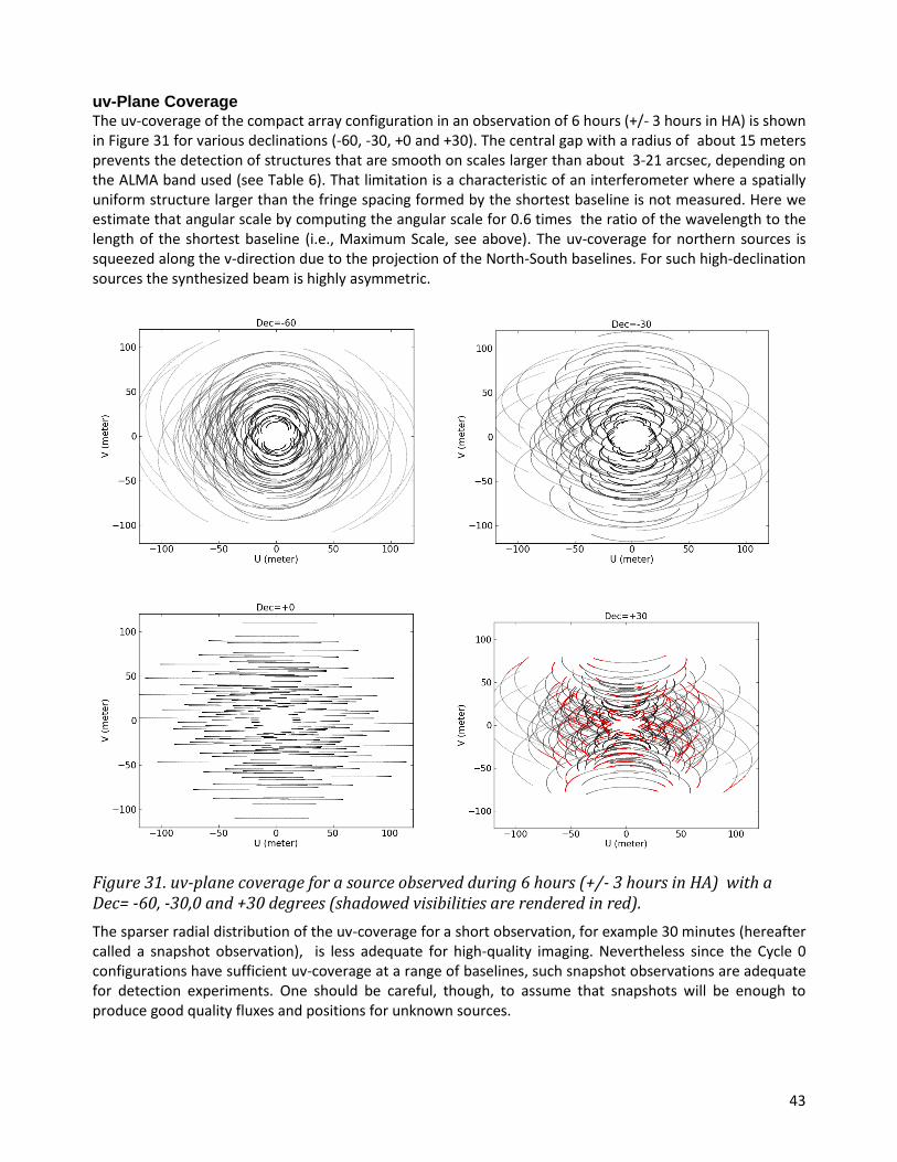
uv-Plane Coverage The uv-coverage of the compact array configuration in an observation of 6 hours (+/- 3 hours in HA) is shown in Figure 31 for various declinations (-60, -30, +0 and +30). The central gap with a radius of about 15 meters prevents the detection of structures that are smooth on scales larger than about 3-21 arcsec, depending on the ALMA band used (see Table 6). That limitation is a characteristic of an interferometer where a spatially uniform structure larger than the fringe spacing formed by the shortest baseline is not measured. Here we estimate that angular scale by computing the angular scale for 0.6 times the ratio of the wavelength to the length of the shortest baseline (i.e., Maximum Scale, see above). The uv-coverage for northern sources is squeezed along the v-direction due to the projection of the North-South baselines. For such high-declination sources the synthesized beam is highly asymmetric.

Figure 31. uv-plane coverage for a source observed during 6 hours (+/- 3 hours in HA) with a Dec= -60, -30,0 and +30 degrees (shadowed visibilities are rendered in red).

The sparser radial distribution of the uv-coverage for a short observation, for example 30 minutes (hereafter called a snapshot observation), is less adequate for high-quality imaging. Nevertheless since the Cycle 0 configurations have sufficient uv-coverage at a range of baselines, such snapshot observations are adequate for detection experiments. One should be careful, though, to assume that snapshots will be enough to produce good quality fluxes and positions for unknown sources.

44

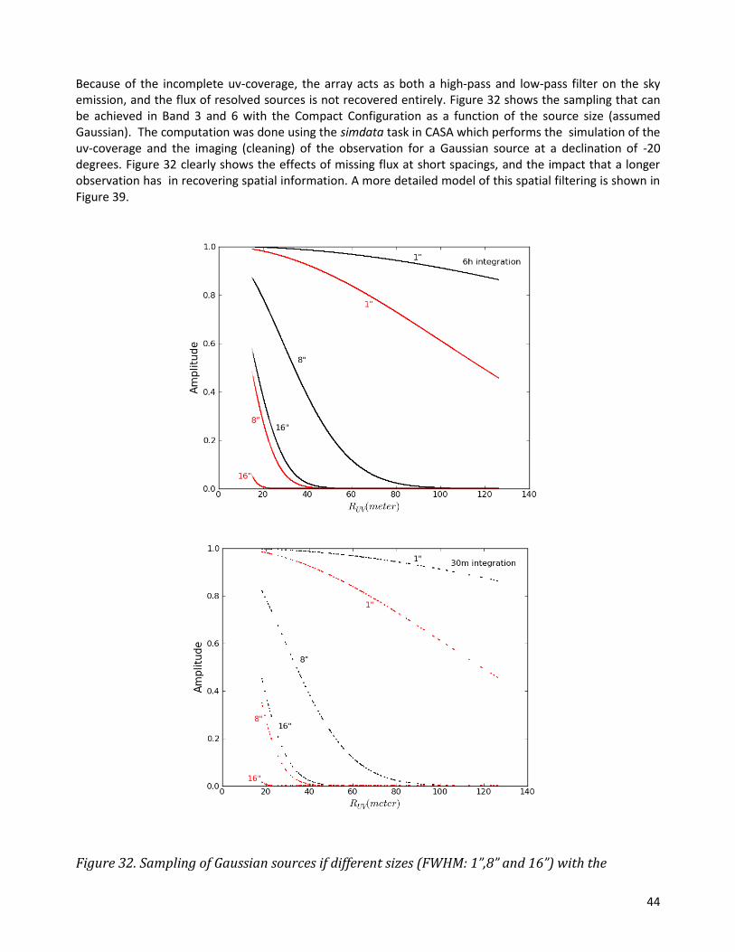
Because of the incomplete uv-coverage, the array acts as both a high-pass and low-pass filter on the sky emission, and the flux of resolved sources is not recovered entirely. Figure 32 shows the sampling that can be achieved in Band 3 and 6 with the Compact Configuration as a function of the source size (assumed Gaussian). The computation was done using the simdata task in CASA which performs the simulation of the uv-coverage and the imaging (cleaning) of the observation for a Gaussian source at a declination of -20 degrees. Figure 32 clearly shows the effects of missing flux at short spacings, and the impact that a longer observation has in recovering spatial information. A more detailed model of this spatial filtering is shown in Figure 39.

Figure 32. Sampling of Gaussian sources if different sizes (FWHM: 1”,8” and 16”) with the

45

Compact Configuration. Black lines are for Band 3 observations at 100 GHz and red lines are for Band 6 observations at 230 GHz. Top plot shows a short observation (30 minutes) and the bottom plot is for a 6 hour (+/- 3h HA) track. The abcissa is the radial distance in the uv-plane

Beam shapes8 The ALMA simulators (see Section 7.1) gives the resulting beam shape for a given antenna configuration and source parameters (input parameters are the observing frequency, declination and duration of observation). Besides the shape of the synthesized beam (FWHM of major and minor axes and orientation) which gives the angular resolution, another important factor is the level of the sidelobes associated with the beam. Sidelobes result from unmeasured portions of the uv plane and are a measure of the magnitude of the defects that must be corrected by any image reconstruction algorithm. An array with lower sidelobes produces more accurate images.

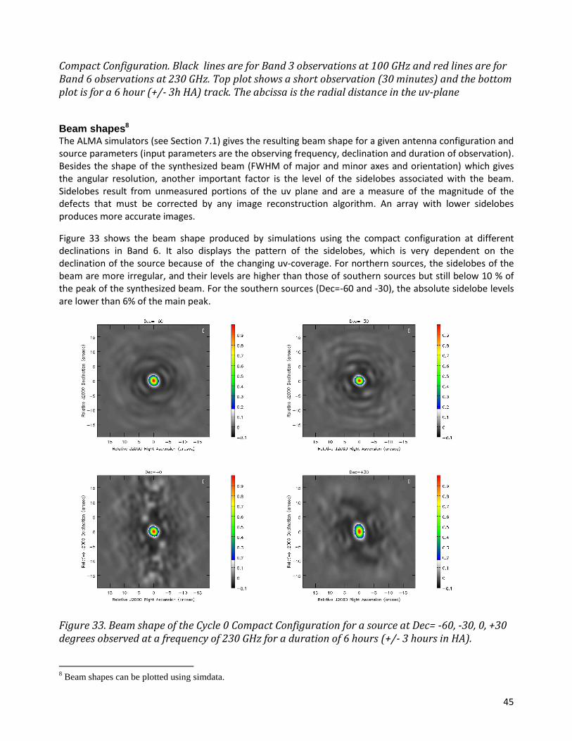
Figure 33 shows the beam shape produced by simulations using the compact configuration at different declinations in Band 6. It also displays the pattern of the sidelobes, which is very dependent on the declination of the source because of the changing uv-coverage. For northern sources, the sidelobes of the beam are more irregular, and their levels are higher than those of southern sources but still below 10 % of the peak of the synthesized beam. For the southern sources (Dec=-60 and -30), the absolute sidelobe levels are lower than 6% of the main peak.

Figure 33. Beam shape of the Cycle 0 Compact Configuration for a source at Dec= -60, -30, 0, +30 degrees observed at a frequency of 230 GHz for a duration of 6 hours (+/- 3 hours in HA).

8 Beam shapes can be plotted using simdata.

46

6.2.2 The Cycle 0 Extended Configuration

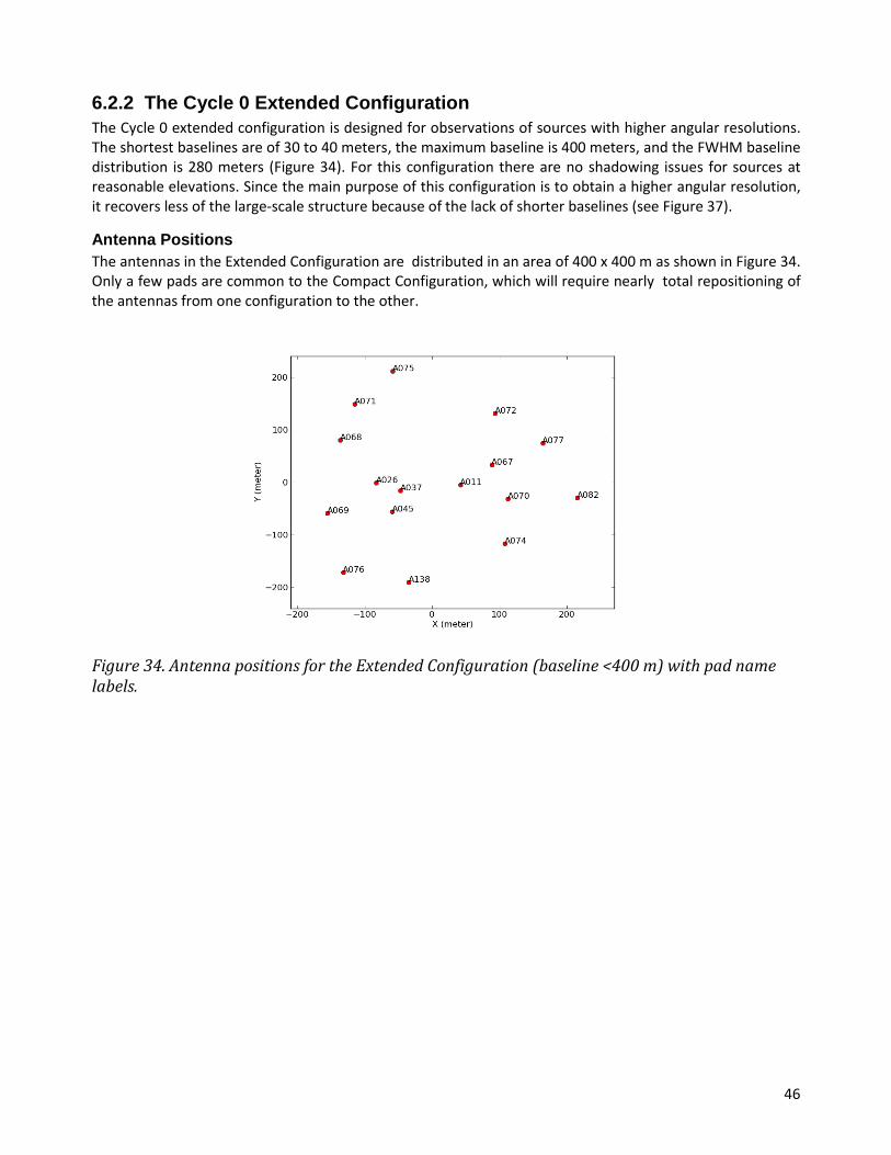
The Cycle 0 extended configuration is designed for observations of sources with higher angular resolutions. The shortest baselines are of 30 to 40 meters, the maximum baseline is 400 meters, and the FWHM baseline distribution is 280 meters (Figure 34). For this configuration there are no shadowing issues for sources at reasonable elevations. Since the main purpose of this configuration is to obtain a higher angular resolution, it recovers less of the large-scale structure because of the lack of shorter baselines (see Figure 37).

Antenna Positions

The antennas in the Extended Configuration are distributed in an area of 400 x 400 m as shown in Figure 34. Only a few pads are common to the Compact Configuration, which will require nearly total repositioning of the antennas from one configuration to the other.

Figure 34. Antenna positions for the Extended Configuration (baseline <400 m) with pad name labels.

47

Figure 35. Radial (top) and azimuth (bottom) density distribution of the data points in the uv-plane, normalized to the total number of visibilities during the observation, for a source with a declination of -30 degree and 6 hours of observation (+/- 3 hours in HA).

uv-Plane Coverage

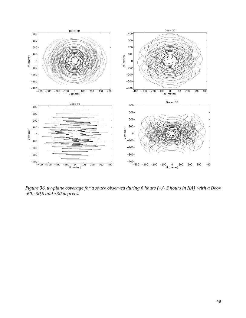
The uv-coverage for the Extended Configuration is shown in Figure 36 for an observation of 6 hours (+/- 3 hours in HA) for sources at different declinations. The dense distribution of baselines shorter than 120 meters (cf. Figure 35 and 36) is apparent at all declinations. Observations of northern sources result in an asymmetric uv-coverage. As for the compact configuration, snapshot observations are sufficient for detection experiments but less adequate for high-quality imaging. The spatial resolution provided by this configuration may be well suited to the imaging of compact sources or structures in fairly crowded fields. The missing low spatial frequencies in the uv-coverage will prevent the proper imaging of extended emission (see Figure 36 and Table 6). A plot of the sampling attained by a short 30 minute observation and a longer 6 hour track is shown in Figure 37 for Bands 3 and 6 and a series of Gaussian sources of different sizes. A more detailed model of the spatial filtering caused by the Extended Configuration is shown in Figure 39.

48

Figure 36. uv-plane coverage for a souce observed during 6 hours (+/- 3 hours in HA) with a Dec= -60, -30,0 and +30 degrees.

49

Figure 37. Sampling of Gaussian sources if different sizes (FWHM: 1”,4” and 7”) with the Extended

Configuration. Black lines are for Band 3 observations at 100 GHz and red lines are for Band 6

50

observations at 230 GHz. Top plot shows a short observation (30 minutes) and the bottom plot is

for a 6 hour (+/- 3h HA) track. The abcissa is the radial distance in the uv-plane.

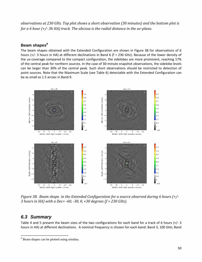
Beam shapes9

The beam shapes obtained with the Extended Configuration are shown in Figure 38 for observations of 6 hours (+/- 3 hours in HA) at different declinations in Band 6 (f = 230 GHz). Because of the lower density of the uv-coverage compared to the compact configuration, the sidelobes are more prominent, reaching 17% of the central peak for northern sources. In the case of 30-minute snapshot observations, the sidelobe levels can be larger than 30% of the central peak. Such short observations should be restricted to detection of point sources. Note that the Maximum Scale (see Table 6) detectable with the Extended Configuration can be as small as 1.5 arcsec in Band 9.

Figure 38. Beam shape in the Extended Configuration for a source observed during 6 hours (+/- 3 hours in HA) with a Dec= -60, -30, 0, +30 degrees (f = 230 GHz).

6.3 Summary Table 4 and 5 present the beam sizes of the two configurations for each band for a track of 6 hours (+/- 3 hours in HA) at different declinations. A nominal frequency is chosen for each band: Band 3, 100 GHz; Band

9 Beam shapes can be plotted using simdata.

51

6, 230 GHz; Band 7, 345 GHz; Band 9, 675 GHz. Table 6 presents the Maximum Scale detectable in each band for the two configurations. It is computed using 0.6 times the ratio of the wavelength to the length of the minimum baseline Lmin (see above).

Table 4. Summary of the spatial resolution, in arcsec, with the minor/major axis of the

synthesized beam for the Compact Configuration (baseline < 125 m)

Band 3 Band 6 Band 7 Band 9

Dec. Maj. Min. Maj. Min. Maj. Min. Maj. Min.

-60 6.0 5.1 2.6 2.2 1.7 1.5 0.9 0.7

-30 5.5 4.8 2.4 2.1 1.6 1.4 0.8 0.7

+0 5.7 5.1 2.5 2.2 1.7 1.5 0.9 0.7

+30 7.8 5.1 3.4 2.2 2.3 1.5 1.2 0.7

Table 5. Summary of the spatial resolution, in arcsec, with the minor/major axis of the synthesized beam for the Extended Configuration (baseline < 400 m) Band 3 Band 6 Band 7 Band 9

Dec. Maj. Min. Maj. Min. Maj. Min. Maj. Min.

-60 1.7 1.5 0.7 0.6 0.5 0.4 0.2 0.2

-30 1.5 1.4 0.6 0.6 0.4 0.4 0.2 0.2

+0 1.6 1.4 0.7 0.6 0.5 0.4 0.2 0.2

+30 2.2 1.5 1.0 0.7 0.6 0.4 0.3 0.2

Table 6. Maximum Scale (arcsec) for a source at Dec = -30 degrees Configuration Compact Extended

Bmin (meter) 15 30

Band 3 (“) 21.0 10.5

Band 6 (“) 9.0 4.5

Band 7 (“) 6.0 3.0

Band 9 (“) 3.0 1.5

52

6.4 Basic Plots of Cycle 0 Observing Parameters and Sensitivities

The figures in this section (Figure 39 to 43) provide an overview of the expected sensitivities for Cycle 0 intended for proposal planning. They are calculated with the sensitivity calculator for central band frequencies: 100 GHz (Band 3), 230 GHz (Band 6), 345 GHz (Band 7) and 675 GHz (Band 9). The actual sensitivities vary over the band as indicated in Section 2.

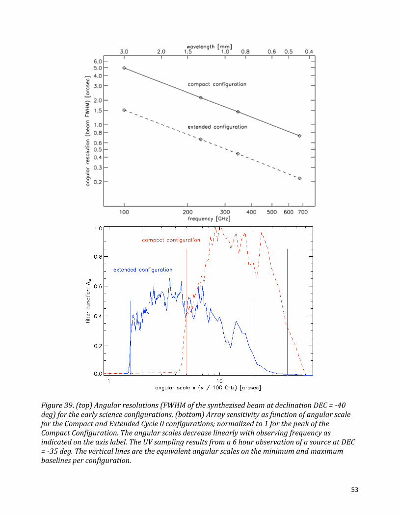
53

Figure 39. (top) Angular resolutions (FWHM of the synthezised beam at declination DEC = -40 deg) for the early science configurations. (bottom) Array sensitivity as function of angular scale for the Compact and Extended Cycle 0 configurations; normalized to 1 for the peak of the Compact Configuration. The angular scales decrease linearly with observing frequency as indicated on the axis label. The UV sampling results from a 6 hour observation of a source at DEC = -35 deg. The vertical lines are the equivalent angular scales on the minimum and maximum baselines per configuration.

54

Figure 40. Precipitable water vapour (PWV) values assumed by the ALMA Sensitivity Calculator for observations in the different ALMA bands. Typically better weather conditions will be chosen for higher frequency bands.

Figure 41. Flux density continuum sensitivity, defined as 5 times the noise RMS, that can be achieved in a 1- hour observation.

55

Figure 42. Brightness continuum sensitivity, defined as 5 times the noise RMS, that can be achieved in a 1 hour observation.

Figure 43. Line sensitivity, defined as 3 times the noise RMS, for a 3 km/s line width that can be achieved in a 4 hour observation.

56

7 Simulations of Cycle 0 observations

7.1 Introduction

7.1.1 The ALMA Simulators

The following two software tools are available to help users simulate the image that might result from an ALMA observation:

The CASA task simdata, which is described in the CASA Manual and from the website at http://casaguides.nrao.edu/index.php?title=Simulated_Observations. The ALMA Observation Support Tool (OST), which is available at the website http://almaost.jb.man.ac.uk/

Both simulators use the sm toolkit package in CASA, and are available from links within the ALMA Science Portal (under Documentation and Tools). The CASA task simdata turns a model of the sky (2 to 4 dimensions including frequency and Stokes) into the visibilities that would be measured by a given configuration of ALMA. The task also can produce a deconvolved (“cleaned”) images of the model visibilities, make a comparison with the input image convolved with the synthesized beam, and calculate a fidelity image10. Simdata can add thermal noise (from receiver, atmosphere, and ground) to the visibilities, and it uses an atmospheric model to calculate atmospheric signal corruption effects (noise) as a function of frequency and site characteristics. The sm CASA toolkit can simulate phase delay variations, gain fluctuations and drift, polarization leakage, and bandpass errors to simulated data. sm also has more flexibility in adding thermal noise than simdata.

OST is a web-based interface to an ALMA maintained by the EU ARC node in Manchester (UK) and at ESO. Like simdata, it is based on the CASA sm toolkit, but uses different wrapper scripts, and in particular, interpolates the atmospheric opacity as a function of frequency from a grid, whereas simdata calculates a new atmospheric profile. Slight differences in atmospheric noise can result. Note that significant differences sometimes exist between the noise predicted by the ALMA Sensitivity Calculator and the measured RMS in the simulated images. These differences are primarily because the RMS measured in an image depends sensitively on the details of how the image is deconvolved. The ALMA sensitivity calculator will be used for the technical assessment of ALMA proposals. Therefore, before using the results from the simulators as a basis of a Technical Justification in an observing proposals, the RMS measured in the simulated image should be rescaled to match the values given by the Sensitivity Calculator.

7.1.2 Basic steps of an ALMA simulation

After installing CASA or entering the OST website, a sky model can be imported and modified with a set of parameters, re-scaling spectral and spatial coordinates and the brightness. The mosaic pointings are calculated and can be saved in a text file, which can be altered or produced externally. Visibilities are calculated for a specific configuration of the ALMA array (input file) on a specific day. The measurements can be ‘corrupted’ by adding thermal and phase noise, cross-polarization, etc. The same atmospheric conditions as in the sensitivity calculator defaults, i.e. 2.7 mm (Band 3), 1.8 mm (Band 6), 1.3 mm (Band 7) and 0.7 mm (Band 9), should be used where noise in the map matters for image reconstruction (it should only be used to

10

Image fidelity = I(x) / | I(x) - T(x) |, where I(x) is the observed image intensity and T(x) is the true image intensity

given the sky model. See also Formula C in the Appendix and ALMA Memo No. 272, available at

http://www.alma.cl/almamemos/.

http://casaguides.nrao.edu/index.php?title=Simulated_Observations

http://almaost.jb.man.ac.uk/

http://www.eso.org/sci/facilities/alma/observing/tools/etc/

http://www.eso.org/sci/facilities/alma/observing/tools/etc/

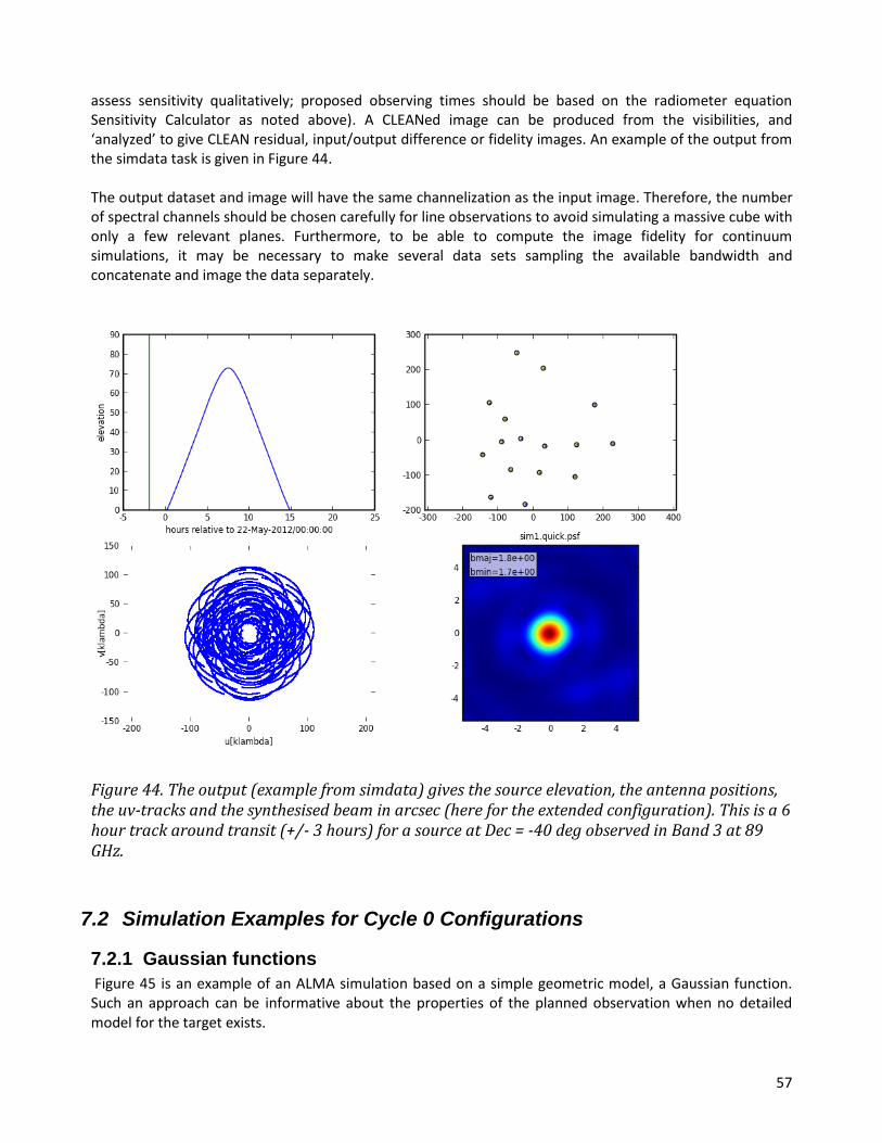
57

assess sensitivity qualitatively; proposed observing times should be based on the radiometer equation Sensitivity Calculator as noted above). A CLEANed image can be produced from the visibilities, and ‘analyzed’ to give CLEAN residual, input/output difference or fidelity images. An example of the output from the simdata task is given in Figure 44. The output dataset and image will have the same channelization as the input image. Therefore, the number of spectral channels should be chosen carefully for line observations to avoid simulating a massive cube with only a few relevant planes. Furthermore, to be able to compute the image fidelity for continuum simulations, it may be necessary to make several data sets sampling the available bandwidth and concatenate and image the data separately.

Figure 44. The output (example from simdata) gives the source elevation, the antenna positions, the uv-tracks and the synthesised beam in arcsec (here for the extended configuration). This is a 6 hour track around transit (+/- 3 hours) for a source at Dec = -40 deg observed in Band 3 at 89 GHz.

7.2 Simulation Examples for Cycle 0 Configurations

7.2.1 Gaussian functions

Figure 45 is an example of an ALMA simulation based on a simple geometric model, a Gaussian function. Such an approach can be informative about the properties of the planned observation when no detailed model for the target exists.

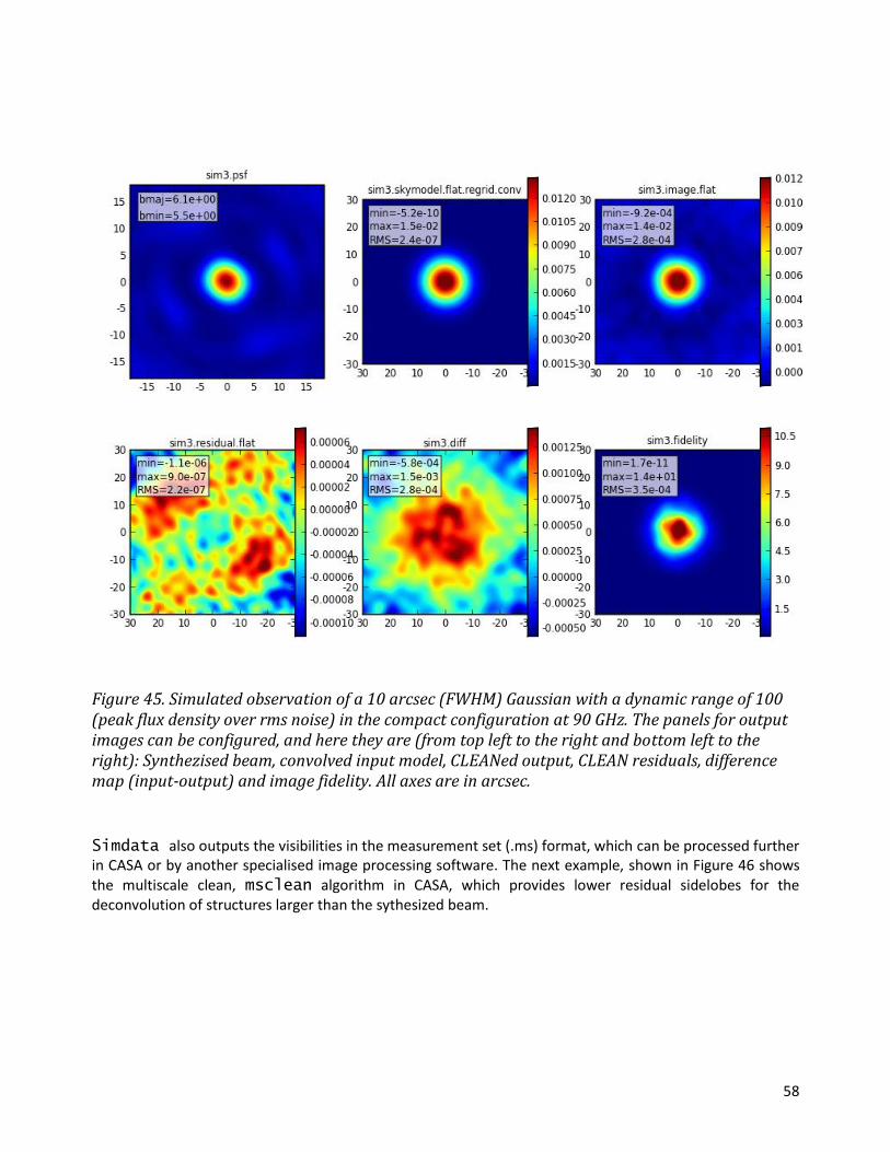
58

Figure 45. Simulated observation of a 10 arcsec (FWHM) Gaussian with a dynamic range of 100 (peak flux density over rms noise) in the compact configuration at 90 GHz. The panels for output images can be configured, and here they are (from top left to the right and bottom left to the right): Synthezised beam, convolved input model, CLEANed output, CLEAN residuals, difference map (input-output) and image fidelity. All axes are in arcsec.

Simdata also outputs the visibilities in the measurement set (.ms) format, which can be processed further in CASA or by another specialised image processing software. The next example, shown in Figure 46 shows the multiscale clean, msclean algorithm in CASA, which provides lower residual sidelobes for the deconvolution of structures larger than the sythesized beam.

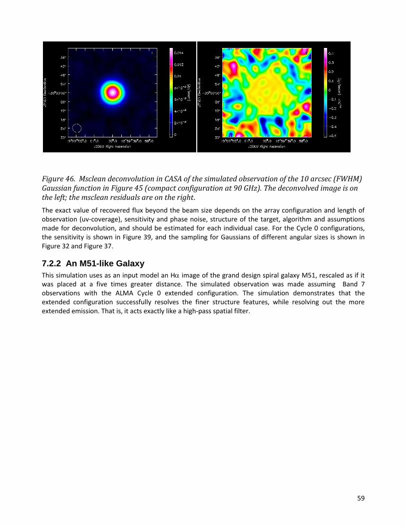
59

Figure 46. Msclean deconvolution in CASA of the simulated observation of the 10 arcsec (FWHM) Gaussian function in Figure 45 (compact configuration at 90 GHz). The deconvolved image is on the left; the msclean residuals are on the right.

The exact value of recovered flux beyond the beam size depends on the array configuration and length of observation (uv-coverage), sensitivity and phase noise, structure of the target, algorithm and assumptions made for deconvolution, and should be estimated for each individual case. For the Cycle 0 configurations, the sensitivity is shown in Figure 39, and the sampling for Gaussians of different angular sizes is shown in Figure 32 and Figure 37.

7.2.2 An M51-like Galaxy

This simulation uses as an input model an H image of the grand design spiral galaxy M51, rescaled as if it was placed at a five times greater distance. The simulated observation was made assuming Band 7 observations with the ALMA Cycle 0 extended configuration. The simulation demonstrates that the extended configuration successfully resolves the finer structure features, while resolving out the more extended emission. That is, it acts exactly like a high-pass spatial filter.

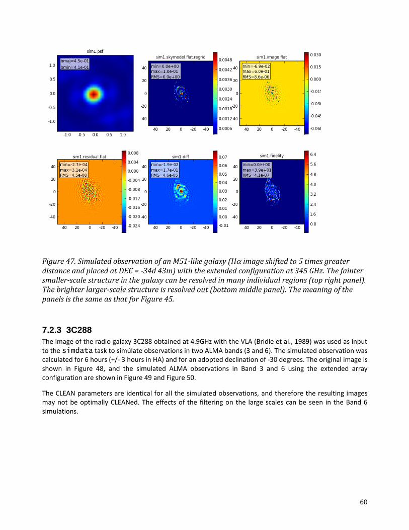
60

Figure 47. Simulated observation of an M51-like galaxy (H image shifted to 5 times greater distance and placed at DEC = -34d 43m) with the extended configuration at 345 GHz. The fainter smaller-scale structure in the galaxy can be resolved in many individual regions (top right panel). The brighter larger-scale structure is resolved out (bottom middle panel). The meaning of the panels is the same as that for Figure 45.

7.2.3 3C288

The image of the radio galaxy 3C288 obtained at 4.9GHz with the VLA (Bridle et al., 1989) was used as input to the simdata task to simúlate observations in two ALMA bands (3 and 6). The simulated observation was calculated for 6 hours (+/- 3 hours in HA) and for an adopted declination of -30 degrees. The original image is shown in Figure 48, and the simulated ALMA observations in Band 3 and 6 using the extended array configuration are shown in Figure 49 and Figure 50.

The CLEAN parameters are identical for all the simulated observations, and therefore the resulting images may not be optimally CLEANed. The effects of the filtering on the large scales can be seen in the Band 6 simulations.

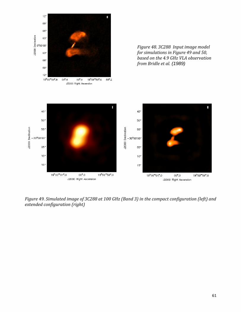
61

Figure 48. 3C288 Input image model for simulations in Figure 49 and 50, based on the 4.9 GHz VLA observation from Bridle et al. (1989)

Figure 49. Simulated image of 3C288 at 100 GHz (Band 3) in the compact configuration (left) and extended configuration (right)

62

Figure 50. Simulated image of 3C288 at 250 GHz (Band 6) in the compact configuration (left) and extended configuration (right).

8 Field Set-up For Cycle 0 single-field interferometry and pointed mosaics (of up to 50 pointings) will be offered. The Single-field interferometry mode also allows observations of arbitrary offset positions with respect to a field center.

Both modes can be set up in the OT during Phase I using the “Field Setup” tab that is defined for each source/science goal. For a general description of the parameters involved in the set-up, refer to the OT User Manual and Reference Manual in the OT itself or following the link: http://almascience.org/document-and-tools.

In this chapter a few examples are provided to illustrate how to use the Field Set-up capabilities in the OT. It is expected that this chapter will be incorporated into the OT manuals in future editions.

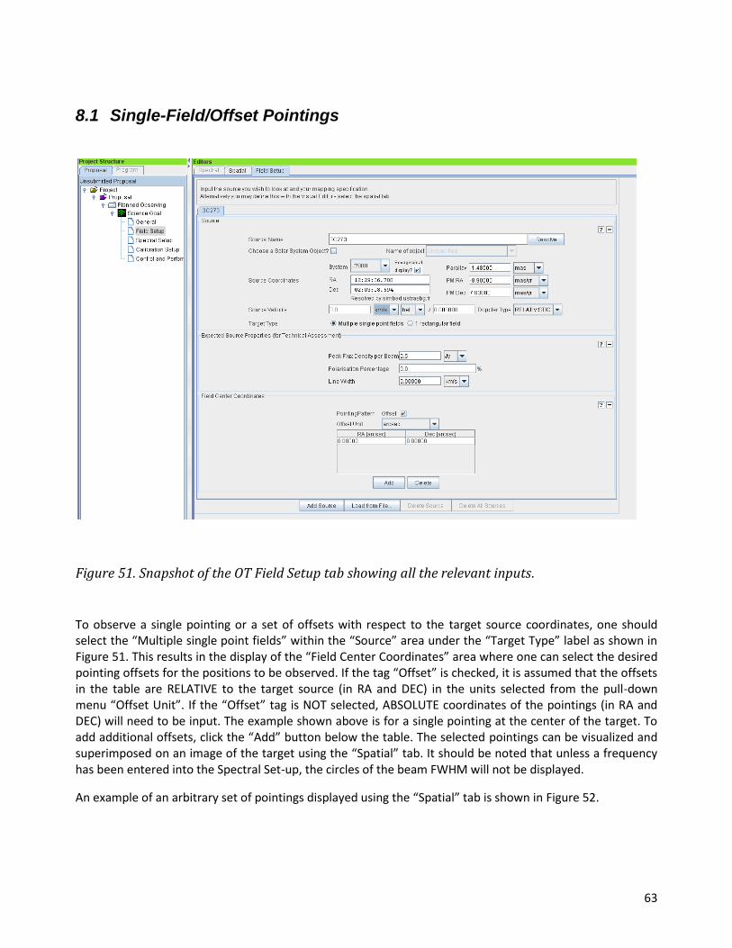
http://almascience.org/document-and-tools

http://almascience.org/document-and-tools

63

8.1 Single-Field/Offset Pointings

Figure 51. Snapshot of the OT Field Setup tab showing all the relevant inputs.

To observe a single pointing or a set of offsets with respect to the target source coordinates, one should select the “Multiple single point fields” within the “Source” area under the “Target Type” label as shown in Figure 51. This results in the display of the “Field Center Coordinates” area where one can select the desired pointing offsets for the positions to be observed. If the tag “Offset” is checked, it is assumed that the offsets in the table are RELATIVE to the target source (in RA and DEC) in the units selected from the pull-down menu “Offset Unit”. If the “Offset” tag is NOT selected, ABSOLUTE coordinates of the pointings (in RA and DEC) will need to be input. The example shown above is for a single pointing at the center of the target. To add additional offsets, click the “Add” button below the table. The selected pointings can be visualized and superimposed on an image of the target using the “Spatial” tab. It should be noted that unless a frequency has been entered into the Spectral Set-up, the circles of the beam FWHM will not be displayed.

An example of an arbitrary set of pointings displayed using the “Spatial” tab is shown in Figure 52.

64

Figure 52. Snapshot of the OT showing the Spatial tab. An example with random pointings is shown for an observing frequency of 86 GHz.

8.2 Square Field To observe a set of adjacent pointings uniformly covering (i.e., providing a Nyquist sampling of 2 samples per beam) a square area in RA and DEC, one has to set the “1 rectangular field” within the “Source” area, under the “Target Type” label as shown in Figure 53.

65

Figure 53. Snapshot of the OT Field Setup tab showing an example of the fields that need to be used to define a rectangular mosaic field.

This results in the display of the “Rectangle” area as shown in Figure 53. There are two possibilities for the coordinates of the pointings, either “Relative” (to the source center as offsets) or “Absolute” (for which the field center in absolute RA and DEC have to be specified). The mosaic can be centered offset from the Source coordinates using the “Field Center Coordinates”. The size, orientation and spacing of the pointings are controlled by the “p & q lenghts”, the “Position Angle”and the “Spacing” inputs. “p” is the the longitude direction and “q” in the latitude direction, respectively. The Position Angle is counted counterclokwise from the longitude axis. It is recommended that the spacings are finer (or equal to) than half a FWHM to avoid undersampling.

As in the case of single-fields, the selected pointings can be visualized (and superimposed on an image of the target” using the “Spatial” tab selectable from the top). Please note that, non-rectangular mosaics will require that the pointings are input using option the “Single-Field/Offset-Pointings” mode described in the previous section. One should remember that if the mosaic spacings are not Nyquist sampled, uniform coverage across the map will not be achieved. An example of a rotated fully-sampled mosaic displayed using the “Spatial” tab is shown in Figure 54.

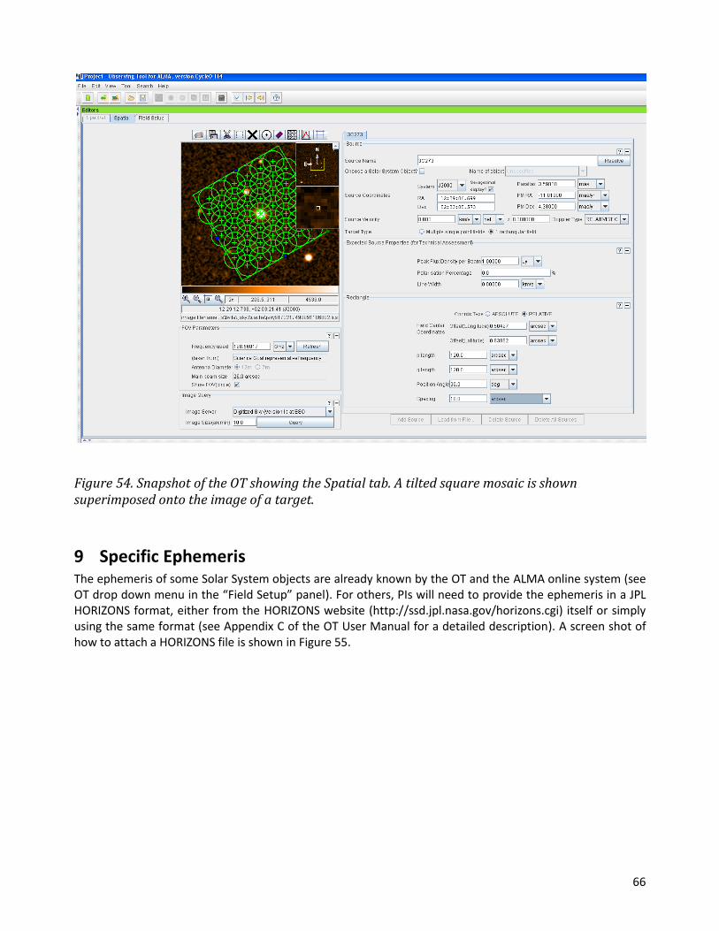
66

Figure 54. Snapshot of the OT showing the Spatial tab. A tilted square mosaic is shown superimposed onto the image of a target.

9 Specific Ephemeris The ephemeris of some Solar System objects are already known by the OT and the ALMA online system (see OT drop down menu in the “Field Setup” panel). For others, PIs will need to provide the ephemeris in a JPL HORIZONS format, either from the HORIZONS website (http://ssd.jpl.nasa.gov/horizons.cgi) itself or simply using the same format (see Appendix C of the OT User Manual for a detailed description). A screen shot of how to attach a HORIZONS file is shown in Figure 55.

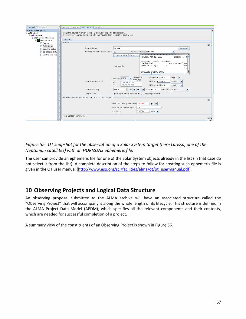
67

Figure 55. OT snapshot for the observation of a Solar System target (here Larissa, one of the Neptunian satellites) with an HORIZONS ephemeris file.

The user can provide an ephemeris file for one of the Solar System objects already in the list (in that case do not select it from the list). A complete description of the steps to follow for creating such ephemeris file is given in the OT user manual (http://www.eso.org/sci/facilities/alma/ot/ot_usermanual.pdf).

10 Observing Projects and Logical Data Structure An observing proposal submitted to the ALMA archive will have an associated structure called the “Observing Project” that will accompany it along the whole length of its lifecycle. This structure is defined in the ALMA Project Data Model (APDM), which specifies all the relevant components and their contents, which are needed for successful completion of a project. A summary view of the constituents of an Observing Project is shown in Figure 56.

http://www.eso.org/sci/facilities/alma/ot/ot_usermanual.pdf

68

Figure 56. Block diagram of an Observing Project from the point of view of the observation preparation (top) and actual execution (bottom). Note that an ObsUnitSet can be composed of other ObsUnitSets as explained in the text. Each time an Schedblock is executed, CONTROL creates a new ExecBlock structure (see text).

69

10.1 Observing Preparation

From the point of view of the proposer, the fundamental unit of the Observing Project is the “Scheduling Block” (hereafter SB). An SB is the smallest sequence of observing instructions that can be scheduled. Scheduling Blocks are produced by the OT (including in Phase 111) and may be edited using the OT in Phase 2 after proposal submission and before/during proposal execution.Projects are broken down into a set of these fundamental units to take maximum advantage of the properties of the ALMA site and the continuously-varying status of the observatory as a whole, including the weather. Each SB has an execution time of typically 30 minutes. Within this time limit, the SB carries out the set-ups, calibrations and target observations to ensure that the acquired data can be properly calibrated and used in the production of the final data product. The end of an SB may be specified in terms of a maximum amount of time or when certain well-defined science goals have been reached. An SB is atomic in the sense that it cannot be re-started in the middle. Therefore, an SB runs to completion, fails, or is terminated by the telescope operators. Structurally, each SB contains two parts, a static and a dynamic part. The dynamic part is a script of observing commands (for standard observing modes it is actually a reference to an external library script) that direct the actual process of observations. The static part consists of fixed auxiliary and meta-data that parameterize the dynamic part. This metadata is generated by the OT during the Phase 2 as part of the SBs. Observations are carried out by interpreting and executing the script supplemented by the relevant parameters contained in the SB.

Given the limited length of the SBs, it often will be necessary to observe several of them to obtain a final image. All the SBs required to reach a specific scientific goal within a project are thus gathered together under a larger structure called an Observing Unit Set (hereafter OUS). An OUS is composed either of a set of SBs or a set of OUS (needed for instance, in the case of the same set of observations for different array configurations). It also contains all the preconditions, performance and calibration requirements, and flow control that apply to that collection. The completion of the parent OUS in each of these triggers reduction of the relevant data by the automated Science Pipeline in Full Science Operations or semi-automated reduction by ALMA staff during Early Science. The only other events that trigger data reduction are at the time of the completion of all the OUS that compose a given Observing Project, or at the end of an observing season, when all the projects are reduced, irrespective of their degree of completion.

10.2 Program Execution

Once a given SB has been selected for execution (by the Scheduler subsystem or by the Array Operator/AoD), it gets loaded into the system and the Control subsystem takes over. The Control subsystem creates an Execution Block structure that is attached to a given SB. Since there is the possibility of the same SB having to be executed several times, many Execution Blocks may exist for a given SB. Each Execution Block contains a record of the parameters and conditions under which the SB was executed along with references to the acquired data.

The internal hierarchical structure of the observations is also shown in Figure 56. The Control subsystem constructs and executes a sequential series of scans. Each scan execution is in fact carried out by breaking it down into a series of subscans, each of which is itself broken into a series of integrations. Although commands are issued at the scan/subscan level, the correlator output corresponds to or is attached to a particular integration. Calibration results from the Telescope Calibration subsystem (TelCal) and QuickLook (QL) pipeline results are usually attached to a subscan. However, some of these results may be accumulated over many subscans, and the resulting object will be attached to the scan to which the subscans belong. The

11

For a description of Phase 1 and Phase 2 see the Cycle 0 Proposer’s Guide

70

Control subsystem is responsible for the creation of all the metadata needed downstream for data processing, for the Execution Block, the scans, subscans and integration objects.

10.3 Structure of an SB and associated scripts

10.3.1 Observing Groups

Within Phase II SBs for a given project, all observing Targets that are to be executed must be included in a “group” within the SB. Each SB can include multiple groups. As of the time of writing, the first group (group 1) of an SB is always the initial calibration group, with subsequent groups detailing the science observation(s). All Science targets and associated calibrators12 within a group are completely observed before the next group is started.

10.3.2 The Standard Interferometry Script

The Cycle 0 observing modes, single field interferometry and pointed mosaics, use the same ALMA observing script, called the “standard interferometry” script. It is designed to provide well-calibrated observations of discrete sources. Within a group, the Science targets are each observed in turn, switching each time that the primary phase calibrator (the calibrator with shortest cycle time in the group) is required to be observed. This means that each science target and associated calibrators in a group may be observed repeatedly within an SB. A set of necessary calibration measurements (e.g. amplitude, bandpass, etc.) specified in group 1 are performed at the beginning of the observation sequence if appropriate sources are available, otherwise this information is collected at the end. Pointing is verified before the amplitude calibrator is observed, and again before the main observations of the science target and phase calibrator cycle. Any additional (“secondary”) phase calibrators are observed as specified in the scheduling block after the primary flux calibrator. Atmospheric calibration to determine system temperature is performed during each iteration of primary phase calibration. For a description of what each calibration entails, see Section 11.

The script is still being developed and may evolve somewhat, but the current version presumes the following group structure and proceeds with the strategy indicated below: Sources: Initial calibration group:

1 Pointing calibrator (near Amplitude calibrator)

1 Amplitude calibrator (typically, Uranus or similar)

1 Atmospheric calibration (near the Amplitude calibrator; in association with the Ampcal and BPcal)

1 Bandpass calibrator

For each subsequent group:

1 (or more) Science targets(s)

1 (or more) Phase calibrator(s)

1 (or more) Pointing source(s) (near to Science target)

1 Atmospheric calibration [associated with the Science target(s) and perhaps also with the Phase calibrator(s)]

Strategy:

12

The user has several options to select optimum calibrators. He/she can let the OT set up adequate queries to the

Calibrator Database in the ALMA Archive. He/she cal also specify the calibrators or set-up the queries.

71

Execute Initial Calibration Group (as necessary): 1. Check Pointing (near Amplitude calibrator) 2. Observe Amplitude calibrator 3. Perform Atmospheric calibration (with a suitable offset from the target) 4. Observe Bandpass calibrator For all other groups: 1. Assume the primary Phase calibrator is the one in the group with the shortest cycle time, and use this to

set the scan duration 2. For each Science target in the group:

2.1. Perform M Pointing calibration observations; M 0 (as determined by the cycle time)

2.2. Perform P Phase calibration observations; P 0 (as determined by the cycle time) 2.3. Perform an Atmospheric calibration (with the hot load) 2.4. Observe the next Science target until complete or a Phase calibration is required 2.5. Perform a primary Phase calibrator observation

3. Repeat until all Science targets are complete or an SB execution time limit is reached; ensure that a final phase calibration is included

10.4 Data and Control Flow

This section describes the overall control of the ALMA system and the flow of data. A summary of the main actors and operations involved in the observations is shown in Figure 57.

Figure 57. Main actors and roles during observations with ALMA. The horizontal direction represents time evolution.

72

Each of the yellow boxes in Figure 57 represent an ALMA subsystem involved in the observations. Orange boxes include labels for the actions performed either by external agents or by those subsystems. A typical observing session would be started by the Telescope Operator interacting with the Executive subsystem via one of the dedicated control computers in the Control Room (the so-called “Standard Test Environment” or STE). The Executive subsystem is in charge of starting up the ALMA Common Software (ACS) and its CORBA-based services and then initializing all of the various software subsystems involved in the observing and data storage process. This is done in several cycles to solve interdependencies between the different software components. Once all the components are ready, the Executive also handles asynchronous events from several of the subsystems and responds to them accordingly. Among the events that it listens to, it is worth mentioning the publication of error conditions to the attention of the operator, and the requests for display of the Control, Telescope Calibration and QuickLook subsystems. The actual observations start by manually creating an array, which means selecting all the antennas that will be involved in the observations. An SB is then selected from the list provided by the Scheduler subsystem, and the execution is started. All the SBs for a given observing season are stored in the Archive after successful Phase 2 completion. The Scheduler subsystem keeps a local up-to-date database of all the SBs (including their status) for a given observing cycle. The Telescope Operator/Astronomer on Duty have two options for using the Scheduler during Early Science. They can either let the Scheduler suggest possible SBs to execute, or they can carry out targeted searches of the local database. For Early Science, the Scheduler can produce a ranked list of optimum SBs to execute next based on weather conditions and forecast, hardware/configuration status, project completion status, representative source position on sky, proposal rank and score and executive percentages. The Telescope Operator/AoD can follow the suggestion of the Scheduler and select one of the top-ranked SBs or something else for execution. Selections that do not follow the advice of the Scheduler must be fully justified by the AoD and will be used to improve the selection algorithm within the Scheduler. It is expected that by Full Operations the algorithm will be optimized to the point that it can run an automatic sequence of SBs without disagreeing with what an AoD would select. Once the execution of the SB has been selected from the Scheduler, it is dispatched to the Control subsystem. Control executes the SB by commanding all relevant hardware and the correlator, resulting in raw data and metadata being made available to the Telescope Calibration (TelCal) and Quick-Look subsystems that report the results/progress/quality of the calibrations carried out during the observations. To carry out its function, Control has many interfaces to the instrumental hardware. It is in fact one of the truly real-time subsystems within ALMA because it is in charge of synchronization of the actions of all antennas (scanning, source acquisition, etc) and correlator to within 48ms (TE). Control is also in charge of storage of data from all monitor points set in the hardware of the ALMA array. Storage of data into the Archive follows two parallel paths and is handled by a part of the Control software called the “Data Capture” module. The best way to describe the Data Capture module is as an interface between the real-time domain of the data taking and the storage side. As an interface, it captures and stores into the Archive all the relevant meta-data information pertaining to a complete description of the data and their supporting calibration and monitor datasets and condenses that information into a set of XML tables. The contents of all these tables are defined in the ALMA Science Data Model (ASDM), which includes a set of 16 core tables (present for all datasets) and up to 30 additional tables (present as needed for a specific observing mode). Together with these tables, Data Capture also creates the relevant links of these metadata to the actual bulk data that is directly stored into the archive. Furthermore, it also provides calibration data

73

to the TelCal and QuickLook subsystems for calibration reduction and display in semi-real time. Finally, when the SB is finished, the Data Capture is in charge of checking that all products representing the raw data have been produced and stored in the archive, and announces the completion of the SB to the Scheduler subsystem. It is clear from the list of roles above that Data Capture is a very complex module, since it has to handle Correlator/backend data, supporting (source information, spectral set-up, etc), and monitoring data needed for the reduction (weather, pointing, etc). All this information originates in different hardware/software elements, each of which can be sampling at different rates and with limited view of the behavior/state of the observing system. A summary plot of the main elements involved in data flow is shown in Figure 58.

Figure 58. Data flow components.

10.5 The ALMA Science Data Model (ASDM) The ASDM defines the collection of information recorded during an observation that is needed for scientific analysis. As described above it contains both bulk binary data and metadata (XML) organized in tables. The tables contain links to other XML tables and addresses pointing to the actual bulk data in the Archive.

The ASDM contains 16 core tables that are common to all observing modes, and up to 23 additional tables that are only created for specific observations. On top of these, the online calibration system (TelCal) also creates associated tables whenever it processes any on the calibrations that can be done on-line. All tables are organized with a similar structure, with the columns listing the contents and the rows including the actual values. The core tables have been defined to outline some of the following: hardware characteristics, array configuration, antenna tracking, the targets, auxiliary monitoring data, overall project and post-processing. A list of the core tables is shown in Figure 59.

74

Figure 59. ASDM Tables. Outlines set of tables are the core ones (i.e., present in all ASDMs).

The associated tables produced by TelCal all have a name starting by “Cal” and then a self-explanatory string on the type of calibration they are associated with. The list of these associated tables is being upgraded as new observing modes/calibrations become available (see Section 11). The current list is shown in Figure 60.

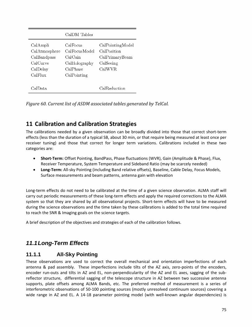
75

Figure 60. Current list of ASDM associated tables generated by TelCal.

11 Calibration and Calibration Strategies The calibrations needed by a given observation can be broadly divided into those that correct short-term effects (less than the duration of a typical SB, about 30 min, or that require being measured at least once per receiver tuning) and those that correct for longer term variations. Calibrations included in these two categories are:

Short-Term: Offset Pointing, BandPass, Phase fluctuations (WVR), Gain (Amplitude & Phase), Flux, Receiver Temperature, System Temperature and Sideband Ratio (may be scarcely needed)

Long-Term: All-sky Pointing (including Band relative offsets), Baseline, Cable Delay, Focus Models, Surface measurements and beam patterns, antenna gain with elevation

Long-term effects do not need to be calibrated at the time of a given science observation. ALMA staff will carry out periodic measurements of these long-term effects and apply the required corrections to the ALMA system so that they are shared by all observational projects. Short-term effects will have to be measured during the science observations and the time taken by these calibrations is added to the total time required to reach the SNR & Imaging goals on the science targets.

A brief description of the objectives and strategies of each of the calibration follows.

11.1 Long-Term Effects

11.1.1 All-Sky Pointing

These observations are used to correct the overall mechanical and orientation imperfections of each antenna & pad assembly. These imperfections include tilts of the AZ axis, zero-points of the encoders, encoder run-outs and tilts in AZ and EL, non-perpendicularity of the AZ and EL axes, sagging of the sub-reflector structure, differential sagging of the telescope structure in AZ between two successive antenna supports, plate offsets among ALMA Bands, etc. The preferred method of measurement is a series of interferometric observations of 50-100 pointing sources (mostly unresolved continuum sources) covering a wide range in AZ and EL. A 14-18 parameter pointing model (with well-known angular dependencies) is

76

fitted to the data and used to derive the required corrections to the nominal pointing positions to correct for all of these structural effects. This all-sky pointing model has a specification RMS of 2” for all ALMA antennas.

11.1.2 Focus Models

Any homologous antenna design causes the optimum focus position to vary as a function of elevation. For a perfect antenna, the only offset that would need to be corrected for would be deflections relative to the axis of the parabolic dish. However, because ALMA deals with off-axis receivers and due to the presence of small non-uniform sagging of the sub-reflector mount/support, corrections in the plane perpendicular to the optical axis are also needed. Models for the offsets of the different ALMA Bands are derived by multiple interferometric/single-dish observations of bright unresolved sources. With these measurements the positions of the maximum power transmission to the receivers as a function of position in three orthogonal directions (X=AZ, Y=EL, Z=optical axis) over a wide range of telescope elevations are derived. The subreflectors are also tilted to maximize the power transfer and avoid reflections of signals originating in the receiver cabin. The reflections are avoided by molding the sub-reflectors with an additional inner conic section.

11.1.3 Baseline

To accurately compute appropiate signal delays, uv sampling, etc, the relative telescope position (i.e., the baseline vector) for all antenna pairs must be known to within a fraction of a wavelength. Baseline determination in ALMA follows a two step approach. An initial estimate of the pad positions is obtained from GPS measurements and/or cartographic maps. Interferometric observations of unresolved continuum sources covering a wide range in hour angle and declination are then used to refine the baseline solutions. It is expected that ALMA will be able to determine baseline vector lengths to an accuracy of 65 μm.

11.1.4 Cable Delay

Errors in the determination of the cable delays from the receiver down to the correlator result in significant slopes of the phase as a function of frequency within a baseband. Determination of the cable delays for all basebands in the two polarizations of a given receiver band is done by interferometrically observing a bright unresolved continuum source and fitting the slope of the phase.

11.1.5 Surface Measurements/Adjustments

The aperture efficiency of an antenna is a very steep function of the ratio of the surface errors (compared to an ideal aperture) to the wavelength of the observations. The practical shortest wavelength an antenna can operate at is given by the surface errors as of about 1/13 of the wavelength. The surface specification for ALMA is 25 μm RMS under all primary operational conditions. The difference between an ideal surface shape and the one of a given antenna is measured with a strong CW (Continuous Wave) signal from a near-field beacon (tower holography at the OSF, and in the future also available at the AOS) and interferometrically using bright celestial sources.This displacement needed to bring the surface panels close to the ideal surface shape are then derived and the panels moved accordingly. .

11.1.6 Beam Patterns

Accurate knowledge of the primary beam patterns, for all ALMA bands and polarizations, is required for imaging, and for understanding telescope performance. They are also needed for correcting beam dilution effects within the FOV of the interferometric observations. Interferometric or SD (Single Dish) observations of bright unresolved sources, obtained by scanning the antenna to be measured in square AZ-EL patterns, are usually used. These allow for the derivation of high SNR maps of the antenna total power beams.

77

11.2 Short-Term Effects

11.2.1 Offset Pointing

To be able to place the sources well within the beams at the highest frequencies offered by ALMA, a pointing accuracy of about 0.6” is needed. This is clearly not possible with the All-Sky Pointing model, and must be measured separately. The strategy is to interferometrically observe nearby pointing calibrators (within 4 degrees of target) at the begining of an SB in order to guarantee the above specification for the typical duration of an SB. These offset pointing measurements will in fact simply update the two collimation offsets (AZ, EL) of the antenna pointing model. When it is not possible to find suitable pointing sources at the highest frequencies (particularly ALMA Bands 7 and 9), a pointing calibrator will be observed in a lower frequency band (Band 3) and these observations along with relative focal plane offsets between receivers will be used to update the offset pointing model.

11.2.2 Bandpass

The spectral response (amplitude and phase) of the combined atmosphere and receiving system is generally not flat for a real interferometric array. It is therefore important to measure the spectral response of the receiving system accurately to the level required by a given observation, as this will be the limiting factor for the accuracy of measurements requiring high spectral dynamical range (especially for high spectral resolution modes). If left uncorrected, the spectral response can leave undesirable chromatic effects across wide spectral bandwidths. At least one bandpass observation should be included per tuning (and per SB if high accuracy is needed). This calibration is done by observing a bright continuum source with a well-known spectral energy distribution (flat-spectrum sources are the easiest to use). A single bandpass is calculated per antenna per polarization. The observation should be long enough to obtain a signal-to-noise on the bandpass calibrator that is at least as high as the desired spectral dynamic range of the target observation.

11.2.3 WVR Corrections:

Fluctuations in the line-of-sight Precipitable Water Vapor (PWV) of two antennas in a given baseline can cause significant decorrelation, especially at the high frequency bands of ALMA. Fluctuations in PWV levels are driven by wind, and can have rapid and strong variations over a large range of spatial scales. All ALMA antennas are equipped with a Water Vapor Radiometer (Dicke-type) that measures at a rate of 1 Hz the emissivity of the atmospheric water line within four spectral bands near 183 GHz. From these measurements, atmospheric models are used to derive the amount of PWV in the line-of-sight and from the difference between the values for the two antennas in a baseline, the phase fluctuations at the observing frequency. A more detailed description of the WVR hardware, specifications and operation can be found in Section 2.3.

11.2.4 Gain (Amplitude & Phase):

The amplitude and phase properties of the atmosphere and receiving system vary more slowly than the PWV fluctuations but vary on timescales of about 10 minutes and are still rapid compared to a typical SB. They are corrected using nearby calibrators (within 10 degs of target). Usually, observations of the science targets are done in cycles of about 15 sec to several minutes (depending on weather conditions, length of the maximum baselines and observing frequency) straddled by observations of the gain calibrators. Ideally the calibrators should be unresolved for simplicity of reduction, but CASA can also cope with resolved calibrators if necessary (using models). Also, phase transfer techniques are possible for gain calibration when using Bands 7 and 9 by using observations of a gain calibrator at Band 3. Phase and gain variations from calibrator observations at Band 3 can be used to derive corrections appropriate for the high frequency bands. Note that phase transfer techniques are only needed whenever there are no adequate calibrators at the high frequency bands. For Cycle 0, the fact that full polarization observations will not be offered implies

78

that there may be some small errors in the observations in those cases where the calibrators used are polarized.

11.2.5 Tsys and Trx

To assess the transparency of the atmosphere at a given observing frequency, the quality of the frequency tuning and to be able to scale the counts that come out of the correlator to brightness temperature units, Tsys must be measured periodically during an SB. ALMA front-ends will be equipped with an Amplitude Calibration Device (ACD) which consists of a robotic arm that can locate two loads of known emissivity temperatures (one at receiver cabin temperature and the other heated to 373 K). Consecutive observations of these two loads and an observation of the sky are used by ALMA to measure the Tsys (see description of the measurements in Section 3.1). The specifications for this calibrations are to reach 1% repeatability for ALMA bands up to 7 and 3% repeatability at higher frequencies.

11.2.6 Amplitude/Flux

Calibration of the data using the Tsys method above does not yield an absolute calibration of the data. It just allows the data to have a high repeatability irrespective of weather conditions, elevation of the observations, etc. To be able to derive an absolute scale of fluxes, observations of “flux standards” are needed. ALMA will observe Solar System objects, bright stars and quasars as primary flux calibrators of well-known properties (i.e., structure and flux as a function of frequency). A measurement of a flux calibrator is needed once per tuning (or per SB if high accuracy is desired). The absolute calibration accuracy for Cycle 0 is 5% for Band 3, 10% for Bands 6 and 7, and 20% for Band 9.

12 Quality Assurance The goal of ALMA Quality Assurance (QA) is to deliver the PI a reliable final data product that is calibrated to the desired accuracy and largely free of calibration or imaging artefacts. For Cycle 0 there are several restrictions that make it a bit more difficult to achieve this goal. It has therefore been decided that QA will also be done on a “best effort” basis, covering all the major issues of the data but may be not completely optimized. Due to the complexity of the ALMA data flow process from SB observations down to the final data merging and reduction at the Science Pipeline, it is important that problems with the system and ill-effects of the environmental conditions are identified and promptly corrected. Otherwise, they would propagate down the dataflow line and could severely affect the data product at the end of the process.

The QA process analysis will be based on a calibration plan that specifies which observations must be acquired and at which intervals in order to monitor system performance and environmental time evolution. Furthermore, it will also tackle issues related to the merging of data taken with different configurations, the inclusion of single-dish data, and the ultimate image quality.

Errors introduced by user-supplied parameters, such as incorrect source coordinates, inadequate frequency setting (e.g. an incorrect redshift), inadequate sensitivity limits (leading to an inadequate integration time or inadequate uv plane coverage, are outside the scope the ALMA QA, unless the error occurred due to faulty information or tools provided by the Observatory.

To be more efficient in detecting problems, ALMA QA has been divided into several stages that mimic the main steps of the data flow. The broad classification of this multi-layered QA approach is:

QA0: At the time of data acquisition

QA1: Observatory-Task Quality Assurance

QA2: Data Reduction

QA3: Post Data Reduction

79

The QA0, 1 and 2 stages will be handled by the Program Management Group (PMG) and the Data Management Group (DMG) (with some contribution from ARC personnel on duty in Chile). The QA3 stage will be handled by the ARCs. The final output of the ALMA QA0-QA2 process is a “QA Report” per project (or ObsUnitSet) that summarizes all the relevant QA information for each of the different QA stages up to the Data Reduction. This report will be included in the data package delivered to the PI. QA3 will be handled separately, as discussed below.

In Chile, responsibility for data quality assurance rests with the Data Manager within the Department of Science Operations, drawing upon the resources of the Program Management Group and the Data Management Group.

A more detailed description of the different stages of QA is as follows:

12.1 What is QA0 and how will it be done?

QA0 is a near-real-time verification of data quality. It deals with rapidly-varying performance parameters (at scales of an SB execution length or shorter) and thus has to be performed at the time of data taking. Assessment is performed by AoDs at the OSF, based on semi-real time output of the calibrations (TelCal) as displayed by Quicklook, and the “Calibration Summary” files that are produced at the end of each SB observation or sequence of SB repeats. This information will be complemented with Monitor and Control display tools to monitor specific parameters not directly tracked by the calibrations (i.e., total power level variations, weather parameters, etc). QA0 metrics/parameters have been selected to check the health of the whole signal path from the atmosphere down to the back-ends. The parameters can be grouped into the following categories:

Atmospheric Effects: Weather Parameters, Sky Opacity, System Temperature, Phase Fluctuations, Total Power Levels, WVR Outputs.

Antenna Issues: Antenna gain, Relative/Offset Pointing, Focus, Antenna Tracking, Geometric Shadowing, Nutators.

Front-End Issues: RF bandpass, Sideband Ratios, Receiver Temperatures, LO lock status. Connectivity Issues: Total Power levels, Delay Measurements, System Temperatures, RF Bandpass, LO lock status.

Back-End Issues: Total Power levels, RF Bandpass, Delay Measurements.

12.2 What is QA1 and how will it be done?

QA1 tackles slowly varying (timescales longer than a week) array performance parameters. They will all be measured by AoDs executing standard calibration SBs created as specified by the Calibration Plan. The QA1-related parameters will, in general, be measured at predefined periods during the month as “Observatory Tasks” and in cases of detection of significant deterioration of performance during operations. Currently the different tasks to measure these parameters are done by different software packages. This situation will be changed in the near future by including most of the packages within TelCal and/or CASA. Reduction of the “Observatory Tasks” will be a joint effort of the AoDs and System Astronomers (DMG). The output of the reduction will be a formatted file including all the information relevant to the specific measurement and including a summary section than can be read by AQUA (ALMA Quality Assurance software) for further processing. The most critical QA1 parameters will also be displayed in real time on the Operations Monitor and Control (OMC) for reference by the AoDs.

The tasks that fall into this category are:

80

Array Calibrations: Baseline measurements, Delays

Antenna Calibrations: All-sky pointing, Focus curves, Surface measurements, Beam patterns (including polarization observations), Relative delays between polarizations of same band

Source Calibrations: Monitoring of flux standards and bootstrapping techniques

12.3 What is QA2 and how will it be done? QA2 deals with QA at the level of the automated data reduction by the Science Pipeline. During Cycle 0, data reduction will be carried out by DSO staff in a semi-automated fashion, using similar scripts to those to be used in later cycles by the automated Pipeline. It is only at the stage of data reduction and analysis of data products that some of the science goals set by the PI can be compared with the results (i.e., SNR, dynamic range, etc). The reduction process may involve merging data, e.g data taken with independent calibrations, or in different configurations. In future cycles, it may also involve combining interferometric and single-dish data. The combined datasets will have to be reduced into a common relative and absolute calibration scale to reflect meaningful physical quantities of the science targets. The combined, calibrated visibilities are then transformed to the image plane and deconvolved using standard algorithms. The resulting images are then checked, using scripts developed by ALMA staff, for the quality of the parameters listed below, and the data are released to the PIs if they fulfill all the acceptable ranges for these QA2 parameters.

The current list of QA2 parameters can be classified as:

Calibration Issues: Relative and Absolute Calibration Quality Among Datasets, Bandpass Calibration (flatness and dynamical range achieved), Overall Gain Calibration (granularity, phase transfer quality, WVR Calibration improvements)

Reduction Process: Data flagging (amount, cause, etc), Cleaning convergence

Final Data products: SNR achieved, Sidelobe levels, Dynamic Range, Contamination by bright sources outside FOV/aliasing, Resolution (spectral & spatial), Comparison of deconvolution algorithms, Residual Structures

Based on these general properties of the errors, merging different datasets requires not only individual self-consistency but also accuracy in their relative calibrations. In particular, datasets taken with the same array in different configurations or at different epochs will need to have comparable quality amplitude (relative and absolute), bandpass and offset pointing calibration observations, since otherwise the merging will not result in improvements of the final imaging products. Similar requirements apply when merging data from different arrays. At the region of uv overlap, the sensitivity should be comparable, or, again, the data with the lower-quality will affect the corresponding uv components and their fidelity in the final image. Additionally, ill-sampling of some of the uv-components (due to some baselines not producing correct data) can cause significant artifacts in the images and even create non-existent structures or decrease the importance of real ones. Finally, the overall absolute scale flux calibration affects any inferences on the actual luminosities of the targets.

12.4 What is QA3 and how will it be done? QA3 is post-reduction evaluation of the data products delivered to the PIs. It will be triggered by PIs using the helpdesk to report any problems with the delivered data products to the ARCs. The ARC receiving the helpdesk report will retrieve the data from the archive and evaluate the nature of the problem. The assessment by the ARC should include BOTH an assessment on whether the problem is present only in a particular dataset or others taken under similar set-ups and conditions also show it. If the problem is deemed to reflect a problem with the performance of the array, the calibration or data reduction process, or

81

the QA process, the ARC will communicate their findings to the DSO, which in return and in collaboration with the ARCs, will work on solving the problem. The result will be communicated back to the reporting investigator. It is expected, due to the restrictions in Cycle 0, that the PIs will play a more active role in the QA process that in later times.

If the problem is of limited impact (i.e., the specific dataset), the dataset would be fully re-reduced using the SCO Science Pipeline and replicated to the ARC Archives after QA. If the problem affects a significant number of datasets so that a re-reduction might significantly slow down the SCO pipeline operations, the ARCs pipelines could be used once a solution has been implemented. The data would then be re-ingested into the SCO Archive and replicated.

13 Data Archiving Data from the correlator, together with additional monitor and weather data, are sent via dedicated optical fiber links (1-10 Gbit/s) to the OSF, where they are archived. The system has been designed to cope with 6.6 MB/s average data rates and 66.6 MB/s peak rates (for short periods of time). The archive at the OSF is designed to provide up to a year of temporary storage for the instrumental data (in the form of “ALMA Science Data Model”, or ASDM, files) and the monitoring data. The instrumental data are then transferred to the main archive at the SCO, where the pipeline is run and from where the data and pipeline products are distributed to the three ALMA Regional Centers (ARCs) in North America, Europe and Japan (Figure 62). The process of copying the data to any of the archives involves a replication of the metadata (support data) and a mirroring of the bulk data (ASDM and FITS files), see Figure 63. These two processes do not need to be simultaneous and they can use different routes (i.e., media delivery and internet). It is expected to use Oracle stream technology for the copies of the metadata.

The ALMA archive consists of two parts - a front-end archive, which is used for storing details of observational scheduling blocks and related data needed to execute observations, and the back-end (science) archive, which stores the instrumental and processed data. The architecture is based on the NGAS system (New Generation Archive System) with Oracle technology for the metadata, as shown in Figure 61.

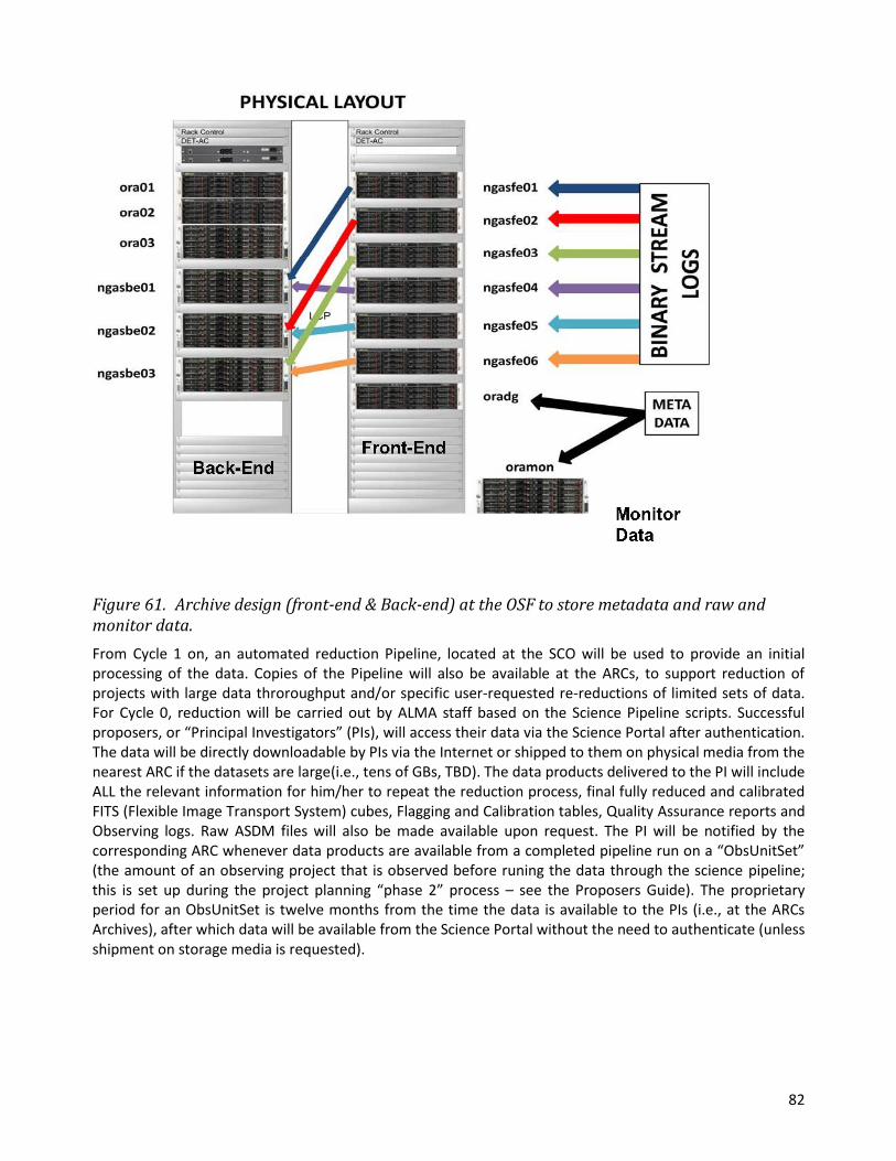
82

Figure 61. Archive design (front-end & Back-end) at the OSF to store metadata and raw and monitor data.

From Cycle 1 on, an automated reduction Pipeline, located at the SCO will be used to provide an initial processing of the data. Copies of the Pipeline will also be available at the ARCs, to support reduction of projects with large data throroughput and/or specific user-requested re-reductions of limited sets of data. For Cycle 0, reduction will be carried out by ALMA staff based on the Science Pipeline scripts. Successful proposers, or “Principal Investigators” (PIs), will access their data via the Science Portal after authentication. The data will be directly downloadable by PIs via the Internet or shipped to them on physical media from the nearest ARC if the datasets are large(i.e., tens of GBs, TBD). The data products delivered to the PI will include ALL the relevant information for him/her to repeat the reduction process, final fully reduced and calibrated FITS (Flexible Image Transport System) cubes, Flagging and Calibration tables, Quality Assurance reports and Observing logs. Raw ASDM files will also be made available upon request. The PI will be notified by the corresponding ARC whenever data products are available from a completed pipeline run on a “ObsUnitSet” (the amount of an observing project that is observed before runing the data through the science pipeline; this is set up during the project planning “phase 2” process – see the Proposers Guide). The proprietary period for an ObsUnitSet is twelve months from the time the data is available to the PIs (i.e., at the ARCs Archives), after which data will be available from the Science Portal without the need to authenticate (unless shipment on storage media is requested).

83

Figure 62. Location of the ALMA archives.

Figure 63. Data flow from the AOS down to the ARCs.

84

14 Appendix

14.1 Antennas At the end of the construction period ALMA will have in total 66 antennas, 54 with a diameter of 12 m and 12 with a diameter of 7 m. Four of the 12 m antennas will be equipped with a nutating subreflector for total power observations. The four antennas used for total power observations and the twelwe 7 m antennas will together form the Atacama Compact Array (ACA). The ALMA antennas are manufactured by three different contractors (one antenna design per ALMA Executive). These are VertexRSI (North America) which will provide 25 12 m antennas, Alcatel Alenia Space European Industrial Engineering MT Aerospace (AEM, Europe), which will provide 25 12 m antennas and Mitsubishi Electric Corporation (MELCO; East Asia), which will provide the four 12 m total power antennas and the twelve 7 m antennas (Figure 64). All antennas have been designed to meet very stringent ALMA performance criteria, and to successfully operate under the extreme environmental conditions at the Array Operation Site (AOS), i.e. strong winds, large temperature ranges and gradients, solar irradiation and snow. The primary operating conditions used for the design of the antennas are the following:

Range of Ambient Temperatures: -20 C <= Tamb <= +20 C

Gradient of temperature: Delta(Tamb) <= 0.6/1.8 C in 10/30 minutes

Wind Velocities: Vwind <= 6/9 m/s (day/night)

Full solar loading

The antennas have the following specifications within the Primary Operating Conditions: Antenna Surface: RMS deviation of 25 microns or less relative to an ideal parabola.

Pointing: Absolute pointing ≤ 2.0 arcsec all-sky. Offset pointing ≤ 0.6 arcsec within a 2 degree radius on the sky.

Primary Beam: The total power pattern response of each ALMA antenna shall be determined to a measurable and repeatable precision better than 1% at frequencies <400 GHz and 2% at frequencies >400 GHz.

Subreflector: 6 degrees of freedom to allow for alignment with the corresponding receiver beam.

Subreflector Motion: Maximum XR and YR displacements of +/- 5 mm. Maximum ZR displacement of +/- 10 mm. The maximum rotation around the and axes is 0.2 degrees. Positioning must be

accurate to 5 microns.

Antenna Location: The phase center position of the ALMA antenna shall be determined to a radial precision of 65 microns (including the antenna structure and pad), stable over two weeks.

Configuration: The ALMA antennas shall be relocatable.

Lifetime: a minimum of 30 years.

All antennas used during ALMA Cycle 0 have 12-meter diameters, with the receivers mounted at the secondary (Cassegrain) focus. The dishes have a focal length, to the primary focus, of 4.8 meters, but the distance from the secondary focus to the plane of the subreflector of the 12 m antennas is 6000 mm, giving an effective focal ratio f/8, with an effective secondary focal length of 96 m and a plate scale of 2.15" per mm. The subreflector has a diameter of 750 mm. The main reflectors of the ALMA 12 m antennas are composed of hundreds of individual panels. Each panel has up to 5 adjustment screws, which can be used to optimize the surface accuracy of the individual

XR

YR

85

antennas (based on holographic measurements). The surface of the panels are etched to scatter optical and near-infrared solar radiation. The antennas are equipped with a movable aluminum subreflector. Subreflector adjustment is used to maximize the transfer of power into the receivers by compensating for changes in the focus position due to gravitational- and temperature-induced deformations. The backplane of the subreflector is attached to a hexapod that controls its position and orientation. The hexapod has six degrees of freedom, displacement and tilt around the three axes, horizontal (X), vertical (Y) and along the optical axis (Z). All antennas have a Cassegrain cabin that is kept at a constant temperature of 20 degrees Centigrade and contains the receivers, the amplitude calibration device and associated electronics. A shutter protects the inside of the Cassegrain cabin when the antenna is not operating. A membrane transparent to the frequencies that can be observed with ALMA is located below the shutter to prevent airflow from the cabin to the outside when the shutter is open. The current design uses a 0.5 mm thick Gore-Tex membrane. The different antennas use a combination of steel, aluminium, Carbon Fiber Reinforced Plastic (CFRP) and Invar in order to achieve the best compromise between stiffness, robustness, smoothness, and low thermal expansion (see Table 7 for a summary of properties). All antennas have built-in metrology systems, which allow thermal and wind deformations to be computed and corrected. For these purposes, the antennas are fitted with thermal sensors, linear sensors and inclinometers (tiltmeters). The Vertex antennas have a drive system that is gear-driven whereas the AEM and MELCO antennas have magnetically supported direct drives. The antennas are controlled using the ALMA Control Software (ACS). ACS sends instructions to the Antenna Bus Master (ABM) computer, which are then sent to the Antenna Control Unit (ACU) through a CAN bus.

Figure 64. The three different ALMA 12m Antenna designs: Vertex, MELCO and AEM (from left to right).

86

14.2 Antenna Foundations

Figure 65. Structure of an antenna pad (actual pad at the OSF) (left) and detail of antenna anchored to a pad (right).

The antennas are placed on specially-designed concrete pads to guarantee stable orientation and location (Figure 65). All antennas are attached to the pads at three points at the vertices of a triangle. The three points (inserts) are located on a circle centered at the antenna pad with a spacing of 120 degrees. This interface guarantees a position repeatability error of the antenna, considered as a rigid body, not exceeding the values below:

X/Y plane < 2 mm (peak to peak)

Rotation around Z < 30 arcsec (peak to peak)

Parallelism with respect to Z +/- 10 arcsec with respect to Zenith The minimum stiffness which the foundation must exhibit at each insert is:

Vertical stiffness (Z) > 13 x 109 N/m

In X/Y plane > 9 x 109 N/m This stiffness includes the inserts, the concrete pad and the soil. This does neither include the kinematic mount lower part nor it includes the foot of the antenna. The position of the pads are measured to a precision of 65 microns, and then monitored for stability for over two weeks. The pads are equipped with two vaults that contain the power, communication, Local Oscillator (LO) and data transmission cables that are connected once the antenna is placed on the pad.

14.3 Antenna Transportation Antennas are moved from one pad to another using a specially-designed transporter Figure 66, right-hand panel). ALMA has two of these vehicles. They are 20 meters long, 10 meters wide and 6 meters high, and

87

each has 28 tires. The transporter positioning system performs a fine positioning of the antenna before setting it down on the foundation in the 3 in-plane degrees of freedom (x, y, rot –z) and in tilt (rot-x, rot-y). Adjustment in each of the 5 adjustment axes can be done independently. The adjustment range of the antenna positioning system compensates for the inaccuracy of the vehicle position with respect to the antenna foundation (which must be smaller 10 cm) in order to achieve the required antenna positioning accuracy. The antennas can be positioned to within a few millimeters, ensuring accurate placement on the antenna foundation pads. More information on the transporters can be found on the ALMA EPO pages13.

Figure 66. The ALMA array with eight 12-m antennas (left), and an antenna being transported to the

AOS (right).

Table 7. Design Properties of the Different ALMA Antennas

BUS

Number

Rings/

Panels

Panel

Material

Quad

type1 Cabin

Yoke

Pedestal

Drive

System2 Metrology System

3

Vertex

CFRP

Al

Invar

8/264 Al + Steel Steel Gear

4 linear displacement

sensors + 1 two-axis

tiltmeter (above the azimuth

bearing)

Melco CFRP 7/205 Al + Steel Steel Direct

Thermal (Yoke, main dish),

Reference Frame, Torque

feedback, Inclinometer,

Right-and-left resolver

metrology, Wind

direction/velocity metrology

AEM CFRP

Invar 5/120

Nickel

Rhodium x CFRP Steel Direct

86 thermal sensors +

2 tiltmeters in yoke

arms

13

http://www.almaobservatory.org/en/technology/transporters

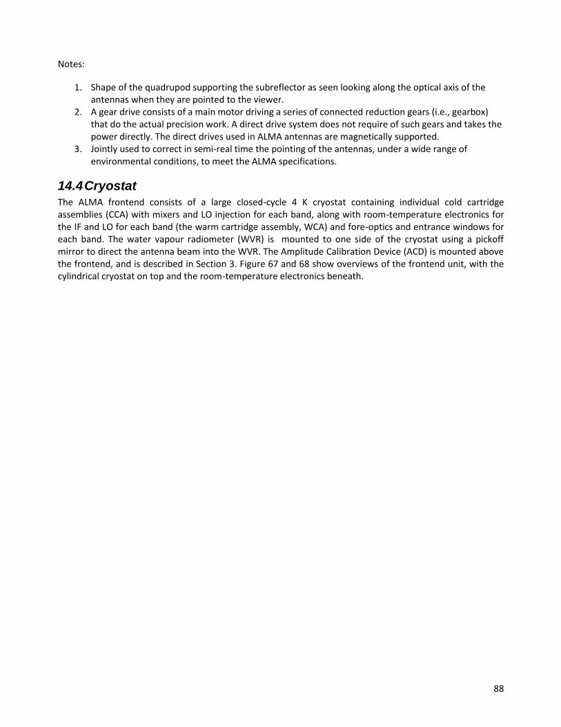
88

Notes:

1. Shape of the quadrupod supporting the subreflector as seen looking along the optical axis of the antennas when they are pointed to the viewer.

2. A gear drive consists of a main motor driving a series of connected reduction gears (i.e., gearbox) that do the actual precision work. A direct drive system does not require of such gears and takes the power directly. The direct drives used in ALMA antennas are magnetically supported.

3. Jointly used to correct in semi-real time the pointing of the antennas, under a wide range of environmental conditions, to meet the ALMA specifications.

14.4 Cryostat

The ALMA frontend consists of a large closed-cycle 4 K cryostat containing individual cold cartridge assemblies (CCA) with mixers and LO injection for each band, along with room-temperature electronics for the IF and LO for each band (the warm cartridge assembly, WCA) and fore-optics and entrance windows for each band. The water vapour radiometer (WVR) is mounted to one side of the cryostat using a pickoff mirror to direct the antenna beam into the WVR. The Amplitude Calibration Device (ACD) is mounted above the frontend, and is described in Section 3. Figure 67 and 68 show overviews of the frontend unit, with the cylindrical cryostat on top and the room-temperature electronics beneath.

89

Figure 67: Side view of ALMA frontend showing cryostat assembly, with room temperature unit below.

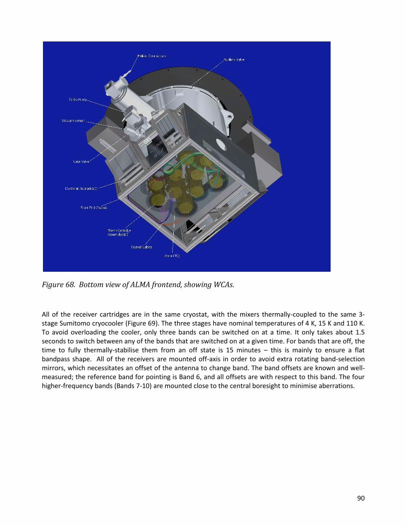
90

Figure 68. Bottom view of ALMA frontend, showing WCAs.

All of the receiver cartridges are in the same cryostat, with the mixers thermally-coupled to the same 3-stage Sumitomo cryocooler (Figure 69). The three stages have nominal temperatures of 4 K, 15 K and 110 K. To avoid overloading the cooler, only three bands can be switched on at a time. It only takes about 1.5 seconds to switch between any of the bands that are switched on at a given time. For bands that are off, the time to fully thermally-stabilise them from an off state is 15 minutes – this is mainly to ensure a flat bandpass shape. All of the receivers are mounted off-axis in order to avoid extra rotating band-selection mirrors, which necessitates an offset of the antenna to change band. The band offsets are known and well-measured; the reference band for pointing is Band 6, and all offsets are with respect to this band. The four higher-frequency bands (Bands 7-10) are mounted close to the central boresight to minimise aberrations.

91

Figure 69. Views of cryostat assembly, showing different windows (top) and the portholes for the WCAs for each band (lower view).

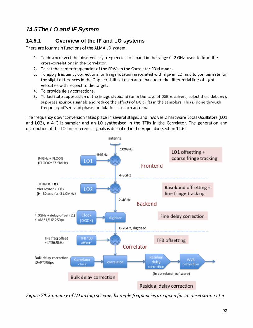
92

14.5 The LO and IF System

14.5.1 Overview of the IF and LO systems

There are four main functions of the ALMA LO system:

1. To downconvert the observed sky frequencies to a band in the range 0–2 GHz, used to form the cross-correlations in the Correlator.

2. To set the center frequencies of the SPWs in the Correlator FDM mode. 3. To apply frequency corrections for fringe rotation associated with a given LO, and to compensate for

the slight differences in the Doppler shifts at each antenna due to the differential line-of-sight velocities with respect to the target.

4. To provide delay corrections. 5. To facilitate suppression of the image sideband (or in the case of DSB receivers, select the sideband),

suppress spurious signals and reduce the effects of DC drifts in the samplers. This is done through frequency offsets and phase modulations at each antenna.

The frequency downconversion takes place in several stages and involves 2 hardware Local Oscillators (LO1 and LO2), a 4 GHz sampler and an LO synthesised in the TFBs in the Correlator. The generation and distribution of the LO and reference signals is described in the Appendix (Section 14.6).

Figure 70. Summary of LO mixing scheme. Example frequencies are given for an observation at a

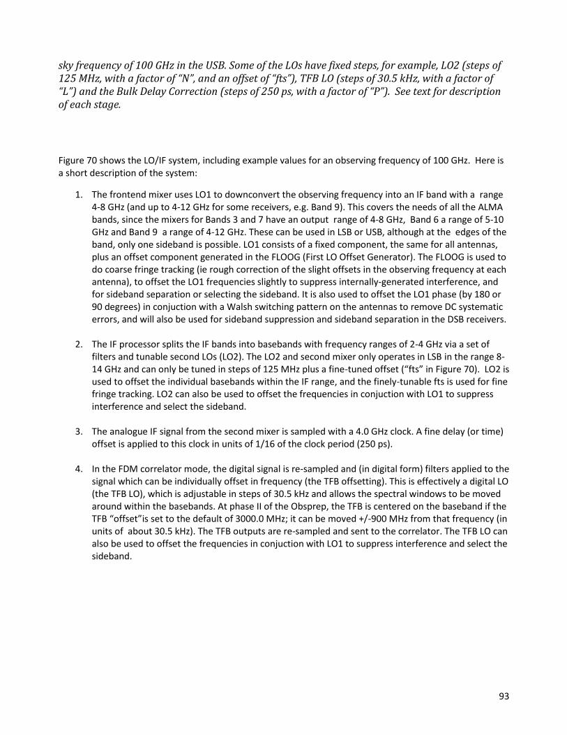
93

sky frequency of 100 GHz in the USB. Some of the LOs have fixed steps, for example, LO2 (steps of 125 MHz, with a factor of “N”, and an offset of “fts”), TFB LO (steps of 30.5 kHz, with a factor of “L”) and the Bulk Delay Correction (steps of 250 ps, with a factor of “P”). See text for description of each stage.

Figure 70 shows the LO/IF system, including example values for an observing frequency of 100 GHz. Here is a short description of the system:

1. The frontend mixer uses LO1 to downconvert the observing frequency into an IF band with a range 4-8 GHz (and up to 4-12 GHz for some receivers, e.g. Band 9). This covers the needs of all the ALMA bands, since the mixers for Bands 3 and 7 have an output range of 4-8 GHz, Band 6 a range of 5-10 GHz and Band 9 a range of 4-12 GHz. These can be used in LSB or USB, although at the edges of the band, only one sideband is possible. LO1 consists of a fixed component, the same for all antennas, plus an offset component generated in the FLOOG (First LO Offset Generator). The FLOOG is used to do coarse fringe tracking (ie rough correction of the slight offsets in the observing frequency at each antenna), to offset the LO1 frequencies slightly to suppress internally-generated interference, and for sideband separation or selecting the sideband. It is also used to offset the LO1 phase (by 180 or 90 degrees) in conjuction with a Walsh switching pattern on the antennas to remove DC systematic errors, and will also be used for sideband suppression and sideband separation in the DSB receivers.

2. The IF processor splits the IF bands into basebands with frequency ranges of 2-4 GHz via a set of filters and tunable second LOs (LO2). The LO2 and second mixer only operates in LSB in the range 8-14 GHz and can only be tuned in steps of 125 MHz plus a fine-tuned offset (“fts” in Figure 70). LO2 is used to offset the individual basebands within the IF range, and the finely-tunable fts is used for fine fringe tracking. LO2 can also be used to offset the frequencies in conjuction with LO1 to suppress interference and select the sideband.

3. The analogue IF signal from the second mixer is sampled with a 4.0 GHz clock. A fine delay (or time)

offset is applied to this clock in units of 1/16 of the clock period (250 ps).

4. In the FDM correlator mode, the digital signal is re-sampled and (in digital form) filters applied to the signal which can be individually offset in frequency (the TFB offsetting). This is effectively a digital LO (the TFB LO), which is adjustable in steps of 30.5 kHz and allows the spectral windows to be moved around within the basebands. At phase II of the Obsprep, the TFB is centered on the baseband if the TFB “offset”is set to the default of 3000.0 MHz; it can be moved +/-900 MHz from that frequency (in units of about 30.5 kHz). The TFB outputs are re-sampled and sent to the correlator. The TFB LO can also be used to offset the frequencies in conjuction with LO1 to suppress interference and select the sideband.

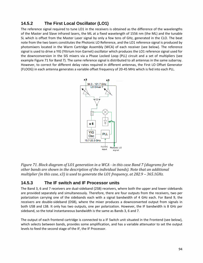
94

14.5.2 The First Local Oscillator (LO1)

The reference signal required to tune LO1 in the receivers is obtained as the difference of the wavelengths of the Master and Slave infrared lasers, the ML at a fixed wavelength of 1556 nm (the ML) and the tunable SL which is offset from the Master Laser signal by only a few tens of GHz, generated in the CLO. The beat note from the two lasers constitutes the Photonic LO Reference, and the LO1 reference signal is produced by photomixers located in the Warm Cartridge Assembly (WCA) of each receiver (see below). The reference signal is used to drive a YIG (Yttrium Iron Garnet) oscillator which produces the LO1 reference signal used for the downconversion in the SIS mixers via a Phase Locked Loop (PLL) circuit and a set of multipliers (see example Figure 71 for Band 7). The same reference signal is distributed to all antennas in the same subarray. However, to correct for different delay rates required in different antennas, the First LO Offset Generator (FLOOG) in each antenna generates a variable offset frequency of 20-45 MHz which is fed into each PLL.

Figure 71. Block diagram of LO1 generation in a WCA - in this case Band 7 (diagrams for the other bands are shown in the description of the individual bands). Note that an additional multiplier (in this case, x3) is used to generate the LO1 frequency, at 282.9 – 365.1GHz.

14.5.3 The IF switch and IF Processor units

The Band 3, 6 and 7 receivers are dual-sideband (2SB) receivers, where both the upper and lower sidebands are provided separately and simultaneously. Therefore, there are four outputs from the receivers, two per polarization carrying one of the sidebands each with a signal bandwidth of 4 GHz each. For Band 9, the receivers are double-sideband (DSB), where the mixer produces a downconverted output from signals in both USB and LSB. It only has two outputs, one per polarization. However, the IF bandwidth is 8 GHz per sideband, so the total instantaneous bandwidth is the same as Bands 3, 6 and 7. The output of each frontend cartridge is connected to a IF Switch unit situated in the Frontend (see below), which selects between bands, provides some amplification, and has a variable attenuator to set the output levels to feed the second stage of the IF, the IF Processor.

95

The four outputs from the IF switch unit are fed into two IF Processor units, one per orthogonal polarization (Figure 72) The IF processors divide the incoming 4-8 GHz IF bands from both sidebands into four 2 GHz basebands and down-convert them to the 2-4 GHz range using the second LO (LO2). Since each baseband is fed by a separate LO2, it is possible to freely locate them within the output bandwidth of the receiver (see Section 5 and Table 8 for limitations). The LO2’s are common to both polarizations which means that both polarizations will have the same spectral setups. The IF processor unit has Total Power detectors for tuning/optimization of the IF power levels into the digital samplers, as well as for some types of observations. Figure 72 shows a simple block diagram of the IF Processor. It is important to note that it is NOT possible to select IF configurations with one baseband in one sideband and three in the other. The LO2s are also used for sideband separation when combined with the first LO (Section 14.5).

Figure 72. Block diagram of IF Processor.

The IF processor provides anti-aliasing filters, which define the 2 GHz baseband width (Section 14.5.4). This results in the higher noise levels on the upper and lower 100 MHz of channels in the TDM correlator mode (see Section 5.4). These filters cause a decrease in the effective IF range to 1.875 GHz.

96

14.5.4 Digitization and Transmission

The outputs of the IF Processor units are fed into the Data Transmission System modules (DTS), that include digitizers and formatters to convert the signals to optical wavelengths for transmission via optical fibers. There are four DTS units per antenna, each one handling data for a given baseband pair (i.e., the same 2 GHz baseband from each of the two orthogonal polarizations). Each baseband is digitized by a separate digitizer at 4 GHz (i.e., Nyquist sampling for a 2 GHz bandwidth), quantizing each sample into 3 bits (8 levels) per polarization, so that a total of 6 bits must be transferred per baseband pair. The digitized signal is then transferred to the formatter part that packages the data in frames of equal size. The output of each DTS module is fed to three optical fibers, each transporting 2 bits, and the signal leaves the antenna after passing through a Fiber Optic Multiplexer (FOM). All DTS modules are fed with reference/timing signals from an associated Digital Clock (DGCK), which is also used to do the fine delay tracking. The outputs of the DTS are sent, via the optical fibers, to the AOS Technical Building where the process is inverted (conversion from optical to digital signal) at the DRXs (Data Receiver units), before the signals are sent to the correlator. Delay corrections due to changes in the length of the optical fibers are done using metadata information to re-align the frames sent from the transmitting side at the antenna (DTX) and the receiving side at the Technical Building (DRX). Figure 73 shows a block diagram of a single DTS module.

Figure 73. The DTX and DRX Signal Digitization and Transmission system.

14.6 Reference and LO Signal Generation and Distribution

The Central Local Oscillator (CLO) system generates and distributes the reference, timing and LO signals to all ALMA components in order to ensure that antenna movement, electronics, and data acquisition are synchronized. The signals are distributed to the antennas through optical fiber using the light of three infrared lasers. Figure 74 shows a block diagram of the CLO.

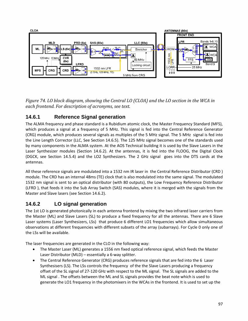
97

Figure 74. LO block diagram, showing the Central LO (CLOA) and the LO section in the WCA in each frontend. For description of acronyms, see text.

14.6.1 Reference Signal generation

The ALMA frequency and phase standard is a Rubidium atomic clock, the Master Frequency Standard (MFS), which produces a signal at a frequency of 5 MHz. This signal is fed into the Central Reference Generator (CRG) module, which produces several signals as multiples of the 5 MHz signal. The 5 MHz signal is fed into the Line Length Corrector (LLC, See Section 14.6.5). The 125 MHz signal becomes one of the standards used by many components in the ALMA system. At the AOS Technical building it is used by the Slave Lasers in the Laser Synthesizer modules (Section 14.6.2). At the antennas, it is fed into the FLOOG, the Digital Clock (DGCK, see Section 14.5.4) and the LO2 Synthesizers. The 2 GHz signal goes into the DTS cards at the antennas.

All these reference signals are modulated into a 1532 nm IR laser in the Central Reference Distributor (CRD ) module. The CRD has an internal 48ms (TE) clock that is also modulated into the same signal. The modulated 1532 nm signal is sent to an optical distributor (with 80 outputs), the Low Frequency Reference Distributor (LFRD ), that feeds it into the Sub Array Switch (SAS) modules, where it is merged with the signals from the Master and Slave lasers (see Section 14.6.2).

14.6.2 LO signal generation

The 1st LO is generated photonically in each antenna frontend by mixing the two infrared laser carriers from the Master (ML) and Slave Lasers (SL) to produce a fixed frequency for all the antennas. There are 6 Slave Laser systems (Laser Synthesizers, LSs) that produce 6 different LO1 frequencies which allow simultaneous observations at different frequencies with different subsets of the array (subarrays). For Cycle 0 only one of the LSs will be available. The laser frequencies are generated in the CLO in the following way:

The Master Laser (ML) generates a 1556 nm fixed optical reference signal, which feeds the Master Laser Distributor (MLD) – essentially a 6-way splitter.

The Central Reference Generator (CRG) produces reference signals that are fed into the 6 Laser Synthesisers (LS). The LSs controls the frequency of the the Slave Lasers producing a frequency offset of the SL signal of 27-120 GHz with respect to the ML signal. The SL signals are added to the ML signal . The offsets between the ML and SL signals provides the beat note which is used to generate the LO1 frequency in the photomixers in the WCAs in the frontend. It is used to set up the

98

LO1 frontend observing frequency, and is set by the software. With 6 LSs it is possible to generate 6 separate LO1 frequencies for the different subarrays.

The Photonic Reference Distribution (PRD) feeds the optical signals to the Sub Array Switch (SAS) which can distribute the signals to the different subarrays,

Both the reference signals and the LO signals are fed through the Line Length Corrector (LLC), which is used to correct for changes in the optical fibres. The LLCs are described in Section 14.6.5.

14.6.3 Optical Signal Distribution

Figure 75 shows the three laser signals after combination in the Sub Array Switches (SAS). The Master and Slave laser signals have wavelengths of about 1556 nm and the laser carrier signal for the reference signals a wavelength of 1532 nm. The signals are distributed via a single-mode fiber optic line to each of the antennas. The fibres are distributed in buried trenches, and fed into the Cassegrain cabin on each antenna through Az and El fibre wraps.

Figure 75. The ALMA reference signals.

Within each antenna, the optical fibers are split and fed to both the LO Reference Receiver (LORR) for the de-modulation of the reference/timing signals, and the LO Photonic Receiver for the LO Reference signals.

14.6.4 Summary of LO distribution system

In addition to setting LO1, the ALMA LO system has two other components: LO2 (in the IFP) and TFB LO (a digital LO in the correlator tunable filterbanks – see Section 4). Figure 76 shows the components involved in the LO distribution.

99

Figure 76. Summary block diagram of the LO distribution system.

14.6.5 LO Path Length Corrections

TheLO Reference signals are generated at the AOS Technical Building and distributed via optical fibers to all the antennas. To guarantee that the phase of the LO signals is stable during the observations for fibers of up to 15km in length, compensation for the changes has to be done in real time. The method adopted by ALMA

100

is based on a round-trip optical interferometer. Phase fluctuations for an optical fiber transmission system are mainly caused by termal expansión of the fiber and mechanical stresses, which produce birrefringent effects and changes in the absolute polarization of the signals. These changes, in turn, cause differential group propagation delays (PDM) that show up as LO phase jitter. A block diagram of the Line Length Correction system implemented by ALMA is shown in Figure 77.

Figure 77. Block diagram of the Line Length Corrector system for ALMA.

The two-wavelength laser synthesizer signal (master and slave lasers) is adjusted in polarization and mixed at the SubArray Switch (SAS) and then passed through a 3-port polarizing beam splitter assembly (PBS). The polarization is aligned so that all the light passes through the beamsplitter. It then passes through a piezo-driven fiber stretcher assembly and the fiber to the antenna. At the antenna end there is a 3-dB coupler, so that half of the light goes to the turnaround assembly and half to the photomixer in each WCA. The turnaround assembly consists of a fiber frequency shifter (located at the LO Photonic Receiver module) and a Faraday Rotator mirror located within the WCA of the Band 9 cartridge in each Front-end.

The frequency of the signal travelling back to the AOS technical building receives thus twice a frequency shift of 25 MHz, thus it comes back offset by 50 MHz from the original. The Faraday rotator reflects the signal but turns its polarization angle by 90 degrees to the incident polarization. This means that the outgoing and returning light is orthogonal everywhere along the fiber between the PBS and the Faraday Mirror. Back at the PBS, the returning signal is sent to a third port where it is mixed with a sample of the Master Laser reference signal in a low-frequency photodetector. This results in an output at the 50 MHz offset frequency. This output is compared in a phase detector with a 50 MHz reference signal and the phase of the whole loop is kept constant by a servo driving the fiber stretchers.

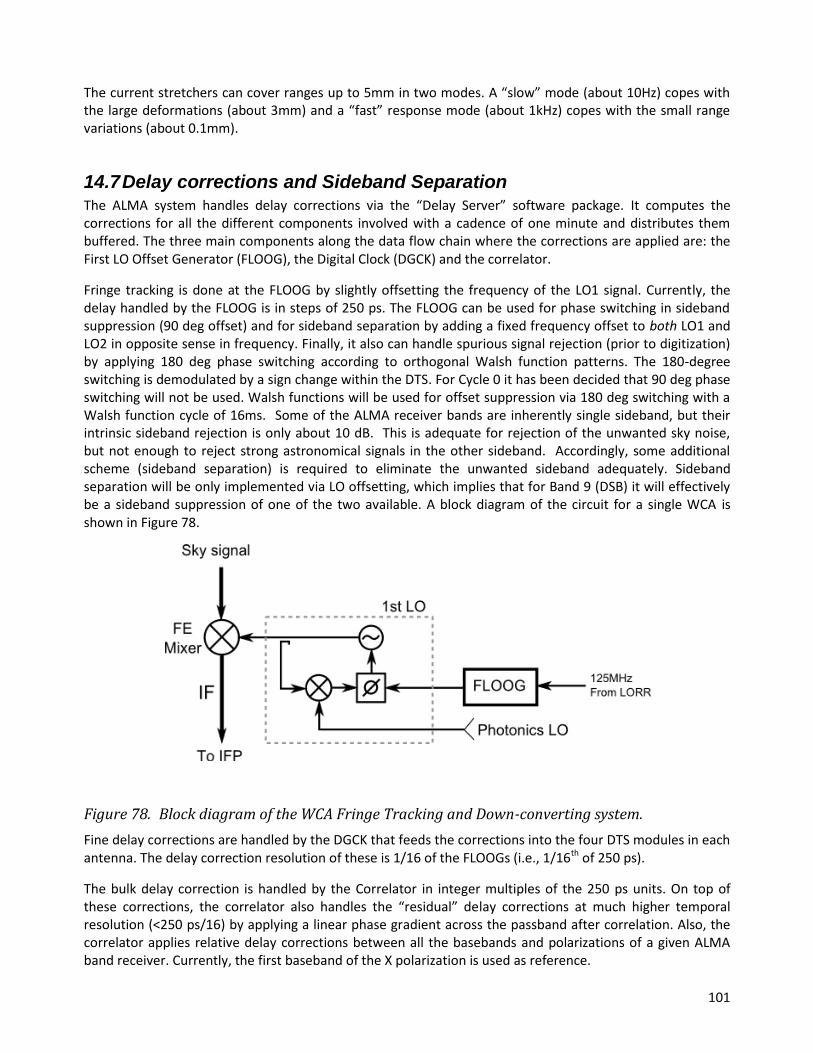
101

The current stretchers can cover ranges up to 5mm in two modes. A “slow” mode (about 10Hz) copes with the large deformations (about 3mm) and a “fast” response mode (about 1kHz) copes with the small range variations (about 0.1mm).

14.7 Delay corrections and Sideband Separation The ALMA system handles delay corrections via the “Delay Server” software package. It computes the corrections for all the different components involved with a cadence of one minute and distributes them buffered. The three main components along the data flow chain where the corrections are applied are: the First LO Offset Generator (FLOOG), the Digital Clock (DGCK) and the correlator.

Fringe tracking is done at the FLOOG by slightly offsetting the frequency of the LO1 signal. Currently, the delay handled by the FLOOG is in steps of 250 ps. The FLOOG can be used for phase switching in sideband suppression (90 deg offset) and for sideband separation by adding a fixed frequency offset to both LO1 and LO2 in opposite sense in frequency. Finally, it also can handle spurious signal rejection (prior to digitization) by applying 180 deg phase switching according to orthogonal Walsh function patterns. The 180-degree switching is demodulated by a sign change within the DTS. For Cycle 0 it has been decided that 90 deg phase switching will not be used. Walsh functions will be used for offset suppression via 180 deg switching with a Walsh function cycle of 16ms. Some of the ALMA receiver bands are inherently single sideband, but their intrinsic sideband rejection is only about 10 dB. This is adequate for rejection of the unwanted sky noise, but not enough to reject strong astronomical signals in the other sideband. Accordingly, some additional scheme (sideband separation) is required to eliminate the unwanted sideband adequately. Sideband separation will be only implemented via LO offsetting, which implies that for Band 9 (DSB) it will effectively be a sideband suppression of one of the two available. A block diagram of the circuit for a single WCA is shown in Figure 78.

Figure 78. Block diagram of the WCA Fringe Tracking and Down-converting system.

Fine delay corrections are handled by the DGCK that feeds the corrections into the four DTS modules in each antenna. The delay correction resolution of these is 1/16 of the FLOOGs (i.e., 1/16th of 250 ps).

The bulk delay correction is handled by the Correlator in integer multiples of the 250 ps units. On top of these corrections, the correlator also handles the “residual” delay corrections at much higher temporal resolution (<250 ps/16) by applying a linear phase gradient across the passband after correlation. Also, the correlator applies relative delay corrections between all the basebands and polarizations of a given ALMA band receiver. Currently, the first baseband of the X polarization is used as reference.

102

14.8 Limitations and rules for spectral setups in Cycle 0

Although the Correlator is will eventually allow for a many complex combinations of SPWs in a single observation, this complexity is being gradually introduced and tested by Commissioning before it is made generally available. In Cycle 0 only a subset of the capabilities have been released. Subsequent Cycles will release more capabilities. Consequently there are several rules (see Table 8) for spectral setups, some of which are general system restrictions, and some of which apply to Cycle 0 (and possibly Cycle 1) only.

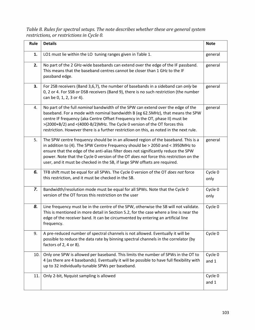
103

Table 8. Rules for spectral setups. The note describes whether these are general system restrictions, or restrictions in Cycle 0.

Rule Details Note

1. LO1 must lie within the LO tuning ranges given in Table 1. general

2. No part of the 2 GHz-wide basebands can extend over the edge of the IF passband. This means that the baseband centres cannot be closer than 1 GHz to the IF passband edge.

general

3. For 2SB receivers (Band 3,6,7), the number of basebands in a sideband can only be 0, 2 or 4. For SSB or DSB receivers (Band 9), there is no such restriction (the number can be 0, 1, 2, 3 or 4).

general

4. No part of the full nominal bandwidth of the SPW can extend over the edge of the baseband. For a mode with nominal bandwidth B (eg 62.5MHz), that means the SPW centre IF frequency (aka Centre Offset Frequency in the OT, phase II) must be >(2000+B/2) and <(4000-B/2)MHz. The Cycle 0 version of the OT forces this restriction. However there is a further restriction on this, as noted in the next rule.

general

5. The SPW centre frequency should be in an allowed region of the baseband. This is a in addition to (4). The SPW Centre Frequency should be > 2050 and < 3950MHz to ensure that the edge of the anti-alias filter does not significantly reduce the SPW power. Note that the Cycle 0 version of the OT does not force this restriction on the user, and it must be checked in the SB, if large SPW offsets are required.

general

6. TFB shift must be equal for all SPWs. The Cycle 0 version of the OT does not force this restriction, and it must be checked in the SB.

Cycle 0

only

7. Bandwidth/resolution mode must be equal for all SPWs. Note that the Cycle 0 version of the OT forces this restriction on the user

Cycle 0

only

8. Line frequency must be in the centre of the SPW, otherwise the SB will not validate. This is mentioned in more detail in Section 5.2, for the case where a line is near the edge of the receiver band. It can be circumvented by entering an artificial line frequency.

Cycle 0

9. A pre-reduced number of spectral channels is not allowed. Eventually it will be possible to reduce the data rate by binning spectral channels in the correlator (by factors of 2, 4 or 8).

Cycle 0

10. Only one SPW is allowed per baseband. This limits the number of SPWs in the OT to 4 (as there are 4 basebands). Eventually it will be possible to have full flexibility with up to 32 individually-tunable SPWs per baseband.

Cycle 0

and 1

11. Only 2-bit, Nyquist sampling is allowed Cycle 0

and 1

104

Documents

ALMA Cycle 0 Technical Handbook - IRAM