Page 1 of 16

TEAMS National Competition

High School Version

Air Quality

25 Questions

Page 2 of 16

Air Filtration

We can think of air pollution in two ways, either as a gas or a particulate. Particulates can range from

dusts to sprays, all of which are solid particles we can measure the concentration of using the following

equation.

Concentration of particulates =Weight of Particulates

Volume of Air through filter

Where the weight of the particle is in microns (𝜇𝑚) and the volume of are through the filter is in m3.

When finding the volume of air through the filter, it is convention to average the air flow to find an

estimate.

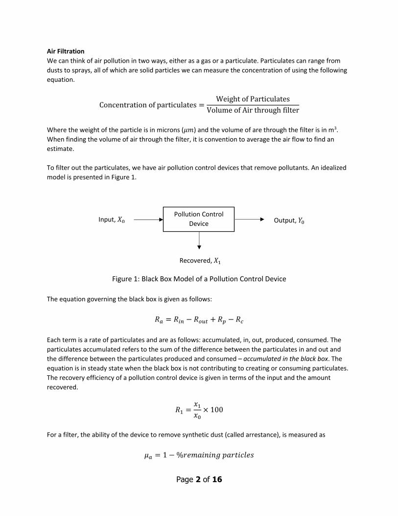
To filter out the particulates, we have air pollution control devices that remove pollutants. An idealized

model is presented in Figure 1.

Figure 1: Black Box Model of a Pollution Control Device

The equation governing the black box is given as follows:

𝑅𝑎 = 𝑅𝑖𝑛 − 𝑅𝑜𝑢𝑡 + 𝑅𝑝 − 𝑅𝑐

Each term is a rate of particulates and are as follows: accumulated, in, out, produced, consumed. The

particulates accumulated refers to the sum of the difference between the particulates in and out and

the difference between the particulates produced and consumed – accumulated in the black box. The

equation is in steady state when the black box is not contributing to creating or consuming particulates.

The recovery efficiency of a pollution control device is given in terms of the input and the amount

recovered.

𝑅1 =𝑥1

𝑥0× 100

For a filter, the ability of the device to remove synthetic dust (called arrestance), is measured as

𝜇𝑎 = 1 − %𝑟𝑒𝑚𝑎𝑖𝑛𝑖𝑛𝑔 𝑝𝑎𝑟𝑡𝑖𝑐𝑙𝑒𝑠

Pollution Control

Device Input, 𝑋0

Recovered, 𝑋1

Output, 𝑌0

Page 3 of 16

Stack Height

If you have ever looked at a factory or live in a city, you have likely seen smoke stacks releasing smoke

into the air – these clouds are called plumes. The dispersion of the pollution is a modeling question that

turns out to be relatively complex due to the dependence of the plume’s shape on the atmospheric

conditions. First, we need to determine how high the plume will be before it begins to bend over –

called the plume rise ∆ℎ.

To calculate the plume rise, we use the following equation:

∆ℎ = 2.6 (𝐹

�̅�𝑆)

13

where �̅� is the average wind speed, S is the stability parameter, and F is the buoyancy flux (m4/s3). The

stability parameter and buoyancy flux are calculated as follows:

𝑆 =𝑔

𝑇𝑎 + 273(

∆𝑇

∆𝑧+ 0.01)

𝐹 =𝑔𝑉𝑠𝑑2(𝑇𝑠 − 𝑇𝑎)

4(𝑇𝑎 + 273)

where g is the gravitational constant (9.81 m/s2), Vs is the stack gas exit velocity (m/s), d is the stack exit

diameter, Ts is the temperature of the stack gas (ᴼC), Ta is the temperature of the atmosphere (ᴼC), and ∆𝑇

∆𝑧 is the lapse rate (ᴼC/m). When added to the original height of the stack, h, we would have the

effective stack height, which is used in the dispersion model.

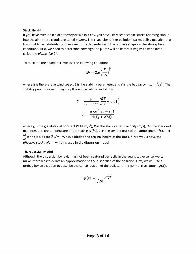
The Gaussian Model

Although the dispersion behavior has not been captured perfectly in the quantitative sense, we can

make inferences to derive an approximation to the dispersion of the pollution. First, we will use a

probability distribution to describe the concentration of the pollutant, the normal distribution 𝜙(𝑥).

𝜙(𝑧) =1

√2𝜋𝑒−

12

𝑧2

Page 4 of 16

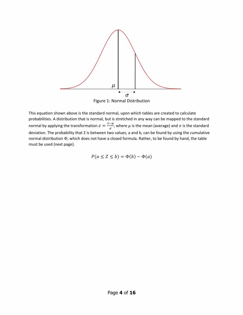
Figure 1: Normal Distribution

This equation shown above is the standard normal, upon which tables are created to calculate

probabilities. A distribution that is normal, but is stretched in any way can be mapped to the standard

normal by applying the transformation 𝑧 =𝑥−𝜇

𝜎, where 𝜇 is the mean (average) and 𝜎 is the standard

deviation. The probability that Z is between two values, a and b, can be found by using the cumulative

normal distribution Φ, which does not have a closed formula. Rather, to be found by hand, the table

must be used (next page).

𝑃(𝑎 ≤ 𝑍 ≤ 𝑏) = Φ(𝑏) − Φ(𝑎)

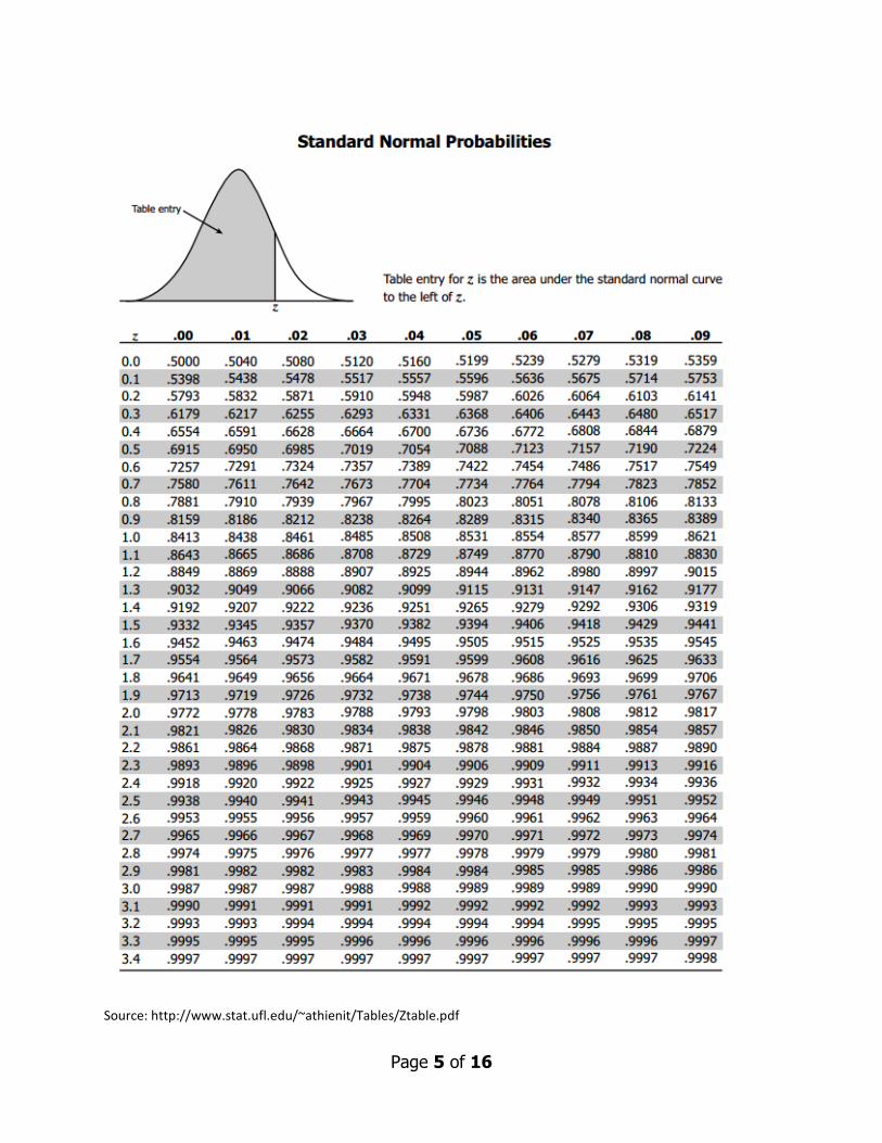
Page 5 of 16

Source: http://www.stat.ufl.edu/~athienit/Tables/Ztable.pdf

Page 6 of 16

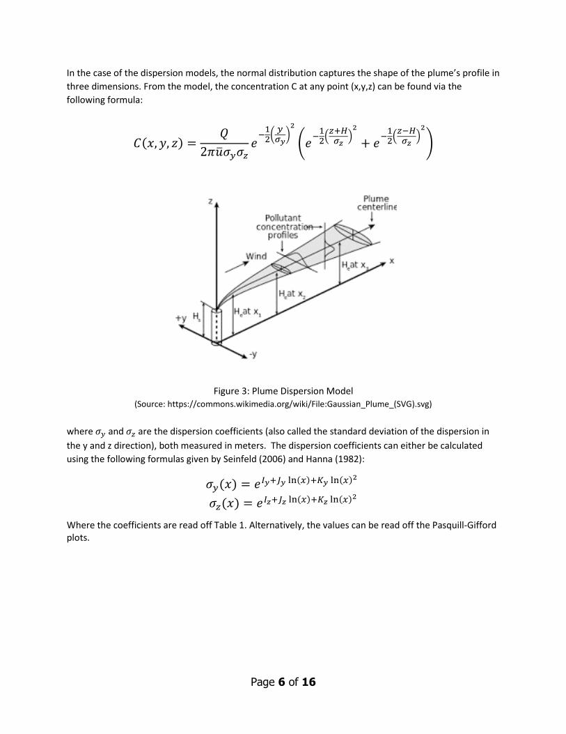
In the case of the dispersion models, the normal distribution captures the shape of the plume’s profile in

three dimensions. From the model, the concentration C at any point (x,y,z) can be found via the

following formula:

𝐶(𝑥, 𝑦, 𝑧) =𝑄

2𝜋�̅�𝜎𝑦𝜎𝑧𝑒

−12

(𝑦

𝜎𝑦)

2

(𝑒−

12

(𝑧+𝐻

𝜎𝑧)

2

+ 𝑒−

12

(𝑧−𝐻

𝜎𝑧)

2

)

Figure 3: Plume Dispersion Model (Source: https://commons.wikimedia.org/wiki/File:Gaussian_Plume_(SVG).svg)

where 𝜎𝑦 and 𝜎𝑧 are the dispersion coefficients (also called the standard deviation of the dispersion in

the y and z direction), both measured in meters. The dispersion coefficients can either be calculated

using the following formulas given by Seinfeld (2006) and Hanna (1982):

𝜎𝑦(𝑥) = 𝑒𝐼𝑦+𝐽𝑦 ln(𝑥)+𝐾𝑦 ln(𝑥)2

𝜎𝑧(𝑥) = 𝑒𝐼𝑧+𝐽𝑧 ln(𝑥)+𝐾𝑧 ln(𝑥)2

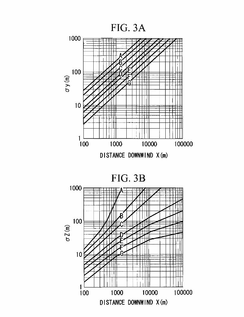
Where the coefficients are read off Table 1. Alternatively, the values can be read off the Pasquill-Gifford plots.

Page 7 of 16

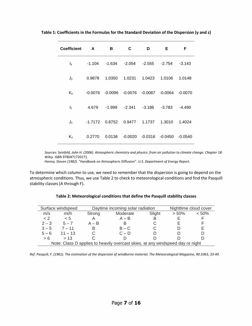
Table 1: Coefficients in the Formulas for the Standard Deviation of the Dispersion (y and z)

Coefficient A B C D E F

Iy -1.104 -1.634 -2.054 -2.555 -2.754 -3.143

Jy 0.9878 1.0350 1.0231 1.0423 1.0106 1.0148

Ky -0.0076 -0.0096 -0.0076 -0.0087 -0.0064 -0.0070

Iz 4.679 -1.999 -2.341 -3.186 -3.783 -4.490

Jz -1.7172 0.8752 0.9477 1.1737 1.3010 1.4024

Kz 0.2770 0.0136 -0.0020 -0.0316 -0.0450 -0.0540

Sources: Seinfeld, John H. (2006). Atmospheric chemistry and physics: from air pollution to climate change. Chapter 18: Wiley. ISBN 9780471720171. Hanna, Steven (1982). "Handbook on Atmospheric Diffusion". U.S. Department of Energy Report.

To determine which column to use, we need to remember that the dispersion is going to depend on the atmospheric conditions. Thus, we use Table 2 to check to meteorological conditions and find the Pasquill stability classes (A through F).

Table 2: Meteorological conditions that define the Pasquill stability classes

Surface windspeed Daytime incoming solar radiation Nighttime cloud cover

m/s mi/h Strong Moderate Slight > 50% < 50% < 2 < 5 A A – B B E F

2 – 3 5 – 7 A – B B C E F 3 – 5 7 – 11 B B – C C D E 5 – 6 11 – 13 C C – D D D D > 6 > 13 C D D D D

Note: Class D applies to heavily overcast skies, at any windspeed day or night

Ref: Pasquill, F. (1961). The estimation of the dispersion of windborne material, The Meteorological Magazine, 90:1063, 33-49.

Page 8 of 16

Concentration of Pollution in a Confined Space

Indoor air quality is paramount to health considering the amount of time we spend indoors, even

though we tend to focus much of our time and attention on outdoor air quality. Many contaminants can

be harmful to us if we breathe too much of it – to name a few: carbon monoxide, asbestos,

formaldehyde.

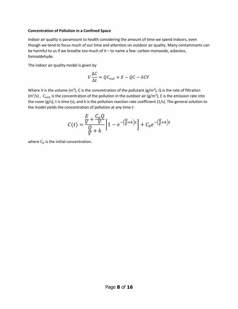
The indoor air quality model is given by

𝑉Δ𝐶

Δ𝑡= 𝑄𝐶𝑜𝑢𝑡 + 𝐸 − 𝑄𝐶 − 𝑘𝐶𝑉

Where V is the volume (m3), C is the concentration of the pollutant (g/m3), Q is the rate of filtration

(m3/s) , 𝐶𝑜𝑢𝑡 is the concentration of the pollution in the outdoor air (g/m3), E is the emission rate into

the room (g/s), t is time (s), and k is the pollution reaction rate coefficient (1/s). The general solution to

the model yields the concentration of pollution at any time t:

𝐶(𝑡) =

𝐸𝑉

+𝐶𝑎𝑄

𝑉𝑄𝑉

+ 𝑘[1 − 𝑒

−(𝑄𝑉

+𝑘)𝑡] + 𝐶0𝑒

−(𝑄𝑉

+𝑘)𝑡

where 𝐶0 is the initial concentration.

Page 9 of 16

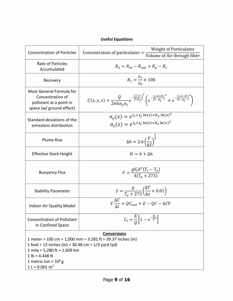
Useful Equations

Concentration of Particles Concentration of particulates =Weight of Particulates

Volume of Air through filter

Rate of Particles Accumulated

𝑅𝑎 = 𝑅𝑖𝑛 − 𝑅𝑜𝑢𝑡 + 𝑅𝑝 − 𝑅𝑐

Recovery 𝑅1 =𝑥1

𝑥0× 100

Most General Formula for Concentration of

pollutant at a point in space (w/ ground effect)

𝐶(𝑥, 𝑦, 𝑧) =𝑄

2𝜋�̅�𝜎𝑦𝜎𝑧𝑒

−12

(𝑦

𝜎𝑦)

2

(𝑒−

12

(𝑧+𝐻

𝜎𝑧)

2

+ 𝑒−

12

(𝑧−𝐻

𝜎𝑧)

2

)

Standard deviations of the emissions distribution

𝜎𝑦(𝑥) = 𝑒𝐼𝑦+𝐽𝑦 ln(𝑥)+𝐾𝑦 ln(𝑥)2

𝜎𝑧(𝑥) = 𝑒𝐼𝑧+𝐽𝑧 ln(𝑥)+𝐾𝑧 ln(𝑥)2

Plume Rise ∆ℎ = 2.6 (𝐹

�̅�𝑆)

13

Effective Stack Height 𝐻 = ℎ + ∆ℎ

Buoyancy Flux

𝐹 =𝑔𝑉𝑠𝑑2(𝑇𝑠 − 𝑇𝑎)

4(𝑇𝑎 + 273)

Stability Parameter 𝑆 =𝑔

𝑇𝑎 + 273(

∆𝑇

∆𝑧+ 0.01)

Indoor Air Quality Model 𝑉Δ𝐶

Δ𝑡= 𝑄𝐶𝑜𝑢𝑡 + 𝐸 − 𝑄𝐶 − 𝑘𝐶𝑉

Concentration of Pollutant in Confined Space

𝐶𝑡 =𝐸

𝑄[1 − 𝑒−

𝑄𝑉

𝑡]

Conversions 1 meter = 100 cm = 1,000 mm = 3.281 ft = 39.37 inches (in) 1 foot = 12 inches (in) = 30.48 cm = 1/3 yard (yd) 1 mile = 5,280 ft = 1.609 km 1 lb = 4.448 N 1 metric ton = 106 g 1 L = 0.001 m3

Page 10 of 16

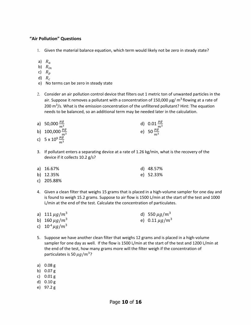
“Air Pollution” Questions

1. Given the material balance equation, which term would likely not be zero in steady state?

a) 𝑅𝑎 b) 𝑅𝑖𝑛 c) 𝑅𝑝

d) 𝑅𝑐 e) No terms can be zero in steady state

2. Consider an air pollution control device that filters out 1 metric ton of unwanted particles in the

air. Suppose it removes a pollutant with a concentration of 150,000 𝜇g/ m3 flowing at a rate of

200 m3/s. What is the emission concentration of the unfiltered pollutant? Hint: The equation needs to be balanced, so an additional term may be needed later in the calculation.

a) 50,000 𝜇𝑔

𝑚3

b) 100,000 𝜇𝑔

𝑚3

c) 5 x 109 𝜇𝑔

𝑚3

d) 0.01 𝜇𝑔

𝑚3

e) 50 𝜇𝑔

𝑚3

3. If pollutant enters a separating device at a rate of 1.26 kg/min, what is the recovery of the

device if it collects 10.2 g/s?

a) 16.67% b) 12.35% c) 205.88%

d) 48.57% e) 52.33%

4. Given a clean filter that weighs 15 grams that is placed in a high-volume sampler for one day and

is found to weigh 15.2 grams. Suppose to air flow is 1500 L/min at the start of the test and 1000 L/min at the end of the test. Calculate the concentration of particulates.

a) 111 𝜇𝑔/𝑚3 b) 160 𝜇𝑔/𝑚3 c) 10-4 𝜇𝑔/𝑚3

d) 550 𝜇𝑔/𝑚3 e) 0.11 𝜇𝑔/𝑚3

5. Suppose we have another clean filter that weighs 12 grams and is placed in a high-volume

sampler for one day as well. If the flow is 1500 L/min at the start of the test and 1200 L/min at the end of the test, how many grams more will the filter weigh if the concentration of particulates is 50 𝜇𝑔/𝑚3?

a) 0.08 g b) 0.07 g c) 0.01 g d) 0.10 g e) 97.2 g

Page 11 of 16

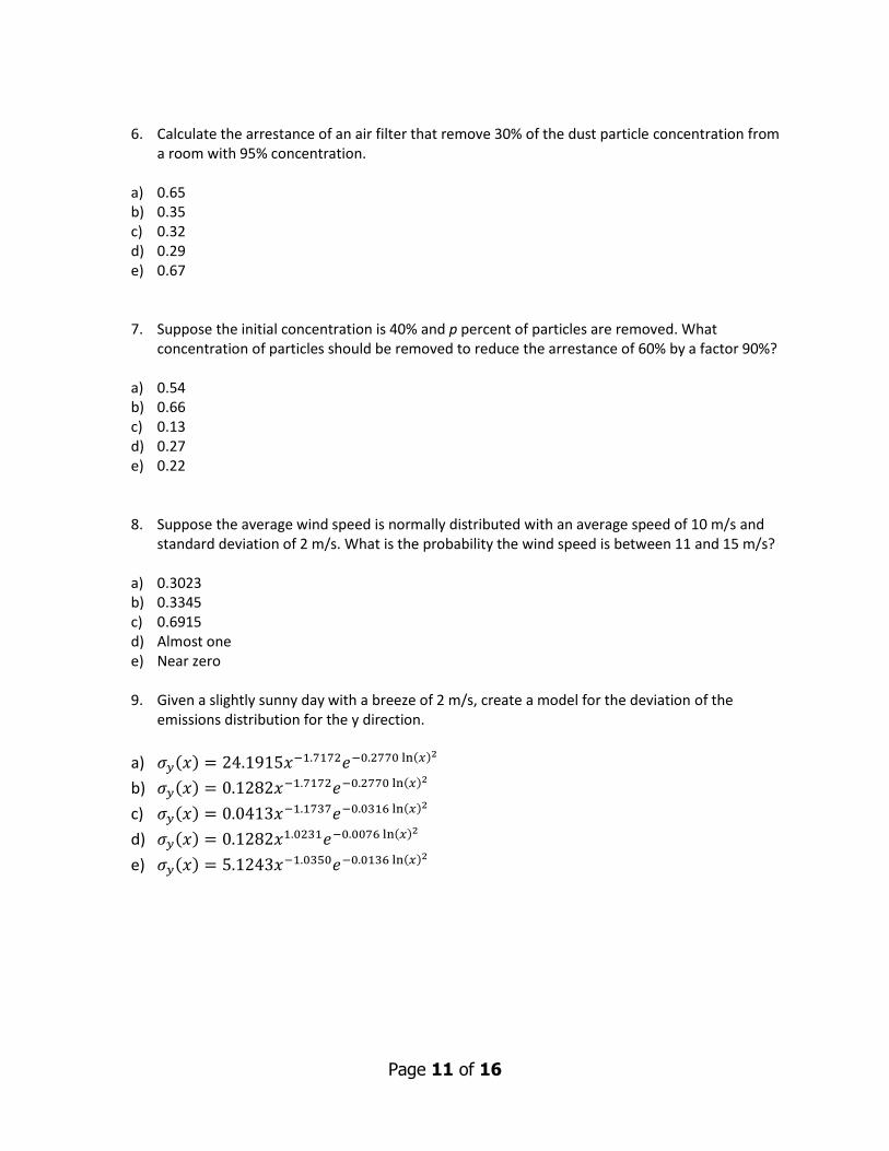
6. Calculate the arrestance of an air filter that remove 30% of the dust particle concentration from

a room with 95% concentration.

a) 0.65 b) 0.35 c) 0.32 d) 0.29 e) 0.67

7. Suppose the initial concentration is 40% and p percent of particles are removed. What concentration of particles should be removed to reduce the arrestance of 60% by a factor 90%?

a) 0.54 b) 0.66 c) 0.13 d) 0.27 e) 0.22

8. Suppose the average wind speed is normally distributed with an average speed of 10 m/s and standard deviation of 2 m/s. What is the probability the wind speed is between 11 and 15 m/s?

a) 0.3023 b) 0.3345 c) 0.6915 d) Almost one e) Near zero

9. Given a slightly sunny day with a breeze of 2 m/s, create a model for the deviation of the

emissions distribution for the y direction.

a) 𝜎𝑦(𝑥) = 24.1915𝑥−1.7172𝑒−0.2770 ln(𝑥)2

b) 𝜎𝑦(𝑥) = 0.1282𝑥−1.7172𝑒−0.2770 ln(𝑥)2

c) 𝜎𝑦(𝑥) = 0.0413𝑥−1.1737𝑒−0.0316 ln(𝑥)2

d) 𝜎𝑦(𝑥) = 0.1282𝑥1.0231𝑒−0.0076 ln(𝑥)2

e) 𝜎𝑦(𝑥) = 5.1243𝑥−1.0350𝑒−0.0136 ln(𝑥)2

Page 12 of 16

Page 13 of 16

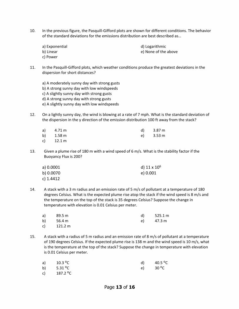
10. In the previous figure, the Pasquill-Gifford plots are shown for different conditions. The behavior of the standard deviations for the emissions distribution are best described as…

a) Exponential b) Linear c) Power

d) Logarithmic e) None of the above

11. In the Pasquill-Gifford plots, which weather conditions produce the greatest deviations in the

dispersion for short distances?

a) A moderately sunny day with strong gusts b) A strong sunny day with low windspeeds c) A slightly sunny day with strong gusts d) A strong sunny day with strong gusts e) A slightly sunny day with low windspeeds

12. On a lightly sunny day, the wind is blowing at a rate of 7 mph. What is the standard deviation of

the dispersion in the y direction of the emission distribution 100 ft away from the stack?

a) 4.71 m b) 1.58 m c) 12.1 m

d) 3.87 m e) 3.53 m

13. Given a plume rise of 180 m with a wind speed of 6 m/s. What is the stability factor if the

Buoyancy Flux is 200?

a) 0.0001 b) 0.0070 c) 1.4412

d) 11 x 106 e) 0.001

14. A stack with a 3 m radius and an emission rate of 5 m/s of pollutant at a temperature of 180

degrees Celsius. What is the expected plume rise atop the stack if the wind speed is 8 m/s and the temperature on the top of the stack is 35 degrees Celsius? Suppose the change in temperature with elevation is 0.01 Celsius per meter.

a) 89.5 m b) 56.4 m c) 121.2 m

d) 525.1 m e) 47.3 m

15. A stack with a radius of 5 m radius and an emission rate of 8 m/s of pollutant at a temperature

of 190 degrees Celsius. If the expected plume rise is 138 m and the wind speed is 10 m/s, what is the temperature at the top of the stack? Suppose the change in temperature with elevation is 0.01 Celsius per meter.

a) 10.3 ᴼC b) 5.31 ᴼC c) 187.2 ᴼC

d) 40.5 ᴼC e) 30 ᴼC

Page 14 of 16

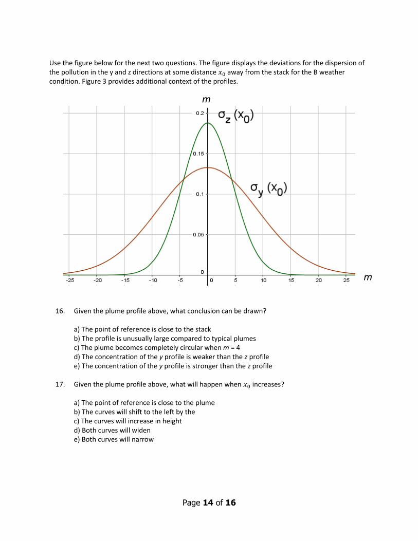
Use the figure below for the next two questions. The figure displays the deviations for the dispersion of the pollution in the y and z directions at some distance 𝑥0 away from the stack for the B weather condition. Figure 3 provides additional context of the profiles.

16. Given the plume profile above, what conclusion can be drawn?

a) The point of reference is close to the stack b) The profile is unusually large compared to typical plumes c) The plume becomes completely circular when m = 4 d) The concentration of the y profile is weaker than the z profile e) The concentration of the y profile is stronger than the z profile

17. Given the plume profile above, what will happen when 𝑥0 increases?

a) The point of reference is close to the plume b) The curves will shift to the left by the c) The curves will increase in height d) Both curves will widen e) Both curves will narrow

m

m

Page 15 of 16

18. Consider a moderately sunny day where the wind is blowing at an average wind speed of 6 m/s.

Suppose a plume is emerging from a stack at ground level at a rate of 0.02 kg/s measured along the center of plume in the y direction. Find the ground level concentration 100 m from the stack. Round deviations to the closest integer.

a) 0.013 g/m3 b) 0.013 kg/m3 c) 0.019 g/m3

d) 0.019 kg/m3 e) 0.038 kg/ m3

19. Consider a 50 m tall stack emitting 0.05 kg/s of pollution with a plume rise of 5 meters above

the stack on a slightly sunny day. Suppose the wind is blowing at an average speed of 1.5 m/s along the x axis. What is the concentration along the direction of the wind 400 meters away from the base of the stack (ignoring ground effects)? Assume the deviations of the dispersion are 68 m in the y direction and 41 in the z direction.

a) 1.92 𝜇g/m3 b) 1.92 mg/m3 c) 2 mg/m3

d) 1.96 mg/m3 e) 1 mg/m3

20. In the previous question, what would the contribution of the ground effect be on the overall

concentration (most nearly)? Round deviations to the closest integer.

a) 0 𝜇g/m3 b) 700 𝜇g/m3 c) 710 𝜇g/m3

d) 715 𝜇g/m3 e) 71 𝜇g/m3

21. Consider a stack with effective height H emitting a pollutant at a rate of Q. If the wind is blowing

at a rate of �̅�, where is the point (x,y,z) at which the pollutant concentration is maximized? Assume H is less than 20 m.

a) (20, 0, H) b) (H, 0, 200) c) (0,0,0) d) (0,H,0) e) (100,H,0)

22. Consider an unvented source of carbon monoxide that has been leaking at a rate of 100𝜇𝑔/𝑠

for approximately 3 hours in a 700 square foot rectangular apartment with 9 foot high ceilings. What is the current concentration of carbon monoxide assuming the initial concentration of CO and the ambient air was zero while the rate of ventilation is 30 L/s?

a) 1 mg/m3 b) 5 x 10-7 mg/m3 c) 3 mg/m3

d) 0.2 mg/m3 e) 3.3 𝜇g/m3

Page 16 of 16

23. Consider the apartment in the previous question, what happens to the concentration when the air filter slowly stops working in the mathematical model?

a) Concentration approaches zero b) Concentration becomes infinite c) Concentration approaches a non-zero value d) Concentration becomes negative e) Concentration increases rapidly proportional to the emission rate 24. Consider an apartment where the time that the carbon monoxide was allowed to fill the room

could vary and increase indefinitely. What is the maximum amount of carbon monoxide that can be in the apartment at any time?

a) E/Q b) Infinity c) Q/V d) V/Q e) exp(-Q/V) Suppose a company designs an air filter that reduces the amount of pollution in the air by k percent per second. If Q(t) is the amount of the pollution in the air in kilograms after t seconds and QP is the amount of pollution produced each second, then the corresponding model is…

∆𝑄(𝑡)

∆𝑡= 𝑄𝑝 −

𝑘

100𝑄(𝑡)

Which is related to the indoor air quality model from which the equation of concentration is derived. 25. What is k if the room is 150 m3 in volume and the filtration rate is 25 L/s?

a) 6 s−1

b) 0.166 s−1

c) 0.0002 s−1

d) 0.02 s−1 e) Not enough information to determine