Embed Size (px)
Citation preview
Chilean Journal of StatisticsVol. 2, No. 1, April 2011, 31–62
Statistics Education
Research Paper
Teaching statistics: Some important tensions
George W. Cobb
Mount Holyoke College, Department of Mathematics and Statistics, Massachusetts, USA
(Received: 26 March 2010 · Accepted in final form: 26 October 2010)
Abstract
Thomas Kuhn’s structure of scientific revolutions (see Kuhn, 1962) identified an essen-tial tension between normal science and paradigm shifts. On a far more modest level,this article identifies several important tensions that confront teachers of statistics, urgesall of us who teach to welcome an opportunity to rethink what we do, and argues, morenarrowly, for replacing the traditional year-long sequence in probability and mathemat-ical statistics with a one-semester course in theory and applications of linear models.Some of the general areas addressed include goals for our students, attitudes towardabstraction, the role of geometric thinking, and attitudes toward mathematics as tooland as aesthetic structure. These are illustrated by comparing different approaches tothe proof of the Gauss-Markov theorem and derivation of sampling distributions.
Keywords: Coordinate free geometry · Gauss-Markov · Herschel-Maxwell · Linearmodels · Mathematical statistics · Statistics education.
Mathematics Subject Classification: Primary 97A99 · Secondary 62J05.
1. Introduction
As statisticians we are scientists, and as scientists we owe a continuing debt to Kuhn (1962,1977) for recognizing and clarifying the role in science of the “essential tension” between“normal science” and times of “paradigm shift”. The paradigm shifts that Kuhn wroteabout were truly seismic, each creating a sudden “world out of joint”. I don’t presume tooffer one of those seismic shifts in this article – at most I may put a few noses out of joint –but Kuhn’s work convinces me that there can be value in regularly questioning tradition,even in much more modest ways. With Kuhn, I suggest that we can benefit by questioningnormal science as part of doing normal science. In the same spirit, we can advance the causeof statistics teaching and learning by identifying and questioning unexamined assumptionsabout what we do, why we do it, and when we do it.My goal in this article is to raise some questions about what I see as the “normal”
way of teaching statistics. In raising these questions, I do not mean to suggest that theconventional way is mistaken, or even necessarily inferior to the alternatives I will describe.Rather, I merely suggest that it can be a useful exercise to rethink the standard ways ofdoing things, and I hope to persuade my readers that there are good reasons to regard
Corresponding address: George W. Cobb. 40 Harris Mountain Road, Amherst, MA 01002, USA.Email: [email protected]
ISSN: 0718-7912 (print)/ISSN: 0718-7920 (online)c⃝ Chilean Statistical Society – Sociedad Chilena de Estadısticahttp://www.soche.cl/chjs
32 G. Cobb
this time of rapid change in our subject as an opportunity to question what we teach asdeeply and broadly as possible.At the same time and in parallel, I will be making an argument for teaching a course in
linear statistical models as a first statistics course for students of mathematics. For manyyears now I have been teaching such a course to undergraduates at Mount Holyoke Collegein Massachusetts. The course requires no previous experience with probability or statistics,only one semester of calculus and one of matrix algebra. Thus it has fewer prerequisitesthan the usual first course in mathematical statistics, and so it can provide an earlier andmore direct path into statistics. Like the course in mathematical statistics, a course inlinear models can be mathematical enough in its content to justify being counted as anupper-division elective in a mathematics major. Unlike the mathematical statistics course,however, a course in linear models can also be a good vehicle for introducing ideas of dataanalysis and statistical modeling.I have made a deliberate decision not to write this article mainly as a description of
the linear models course that I have taught. Such an approach strikes me as unnecessarilynarrow and limiting, because I don’t expect that many readers will end up teaching sucha course, and I would like to think that some of the ideas in this article will be of interestand possible value to colleagues who care about statistics education regardless of whichcourses they teach.In the sections that follow, I structure my thinking as a sequence of choices, a sequence
of tensions between pairs of extremes: about our goals when we teach statistics (Section 2),about how we use abstraction in our teaching (Section 3), about two geometries for rep-resenting data (Section 4), two attitudes toward mathematics (Section 5), and two waysto structure the theory of linear models (Sections 6 and 7). Sections 8 and 9 present, re-spectively, two approaches to the Gauss-Markov theorem and two approaches to samplingdistributions. The article concludes with an argument for the centrality of linear models.
2. Two Kinds of Statistical Challenges
When we teach statistics, what is it that we want our students to learn? Surely the mostcommon answer must be that we want our students to learn to analyze data, and certainlyI share that goal. But for some students, particularly those with a strong interest andability in mathematics, I suggest a complementary goal, one that in my opinion has notreceived enough explicit attention: We want these mathematically inclined students tolearn to solve methodological problems. I call the two goals complementary because, asI shall argue in detail, there are essential tensions between the goals of helping studentslearn to analyze data and helping students learn to solve methodological problems. For aready example of the tension, consider the role of simple, artificial examples. For teachingdata analysis, these “toy” examples are often and deservedly regarded with contempt.But for developing an understanding of a methodological challenge, the ability to create adialectical succession of toy examples and exploit their evolution is critical. As Einstein’sformer research assistant, John Kemeny used to tell his students at Dartmouth: “Thereare two kinds of mathematicians, those who use examples and those who use examples butwon’t admit it”.It is my position in this article that our profession needs (at least) two kinds of statis-
ticians, those who analyze data using methodological solutions devised by others, andthose who care more about devising solutions to methodological challenges than they care
Chilean Journal of Statistics 33
about any one particular data set.1 Our introductory applied course has been evolving,and continues to evolve, in ways that help students learn to analyze data. Our standardintroduction for mathematics majors, the two semester sequence in probability and math-ematical statistics, the course that ought to help students learn to solve methodologicalproblems, has for half a century evolved mainly and sadly in Gould’s punctuated sense,with our typical punctuation mark being a full stop. With a small number of notable ex-ceptions, exceptions that I describe later in this article, the content of today’s books onmathematical statistics is not much changed from that of the pioneering books by Hoel(1947) and Hogg and Craig (1959). Whereas the mathematical statistics course remainsstuck in the curricular tar pits, a course in linear models can offer a vibrant mix of modelingand methodological challenges.The purpose of the following two examples is to illustrate first how a linear models
course lends itself to rich analyses and modeling challenges based on complex data sets,and second how the same course can also be structured as a succession of methodologicalchallenges.
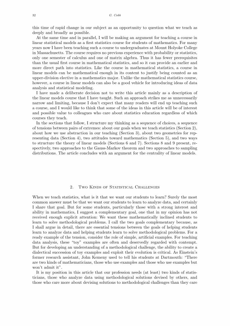
Example 2.1 [Faculty salaries] The scatter plot in Figure 1 plots mean academicsalary versus the percentage of faculty that are women, with points for 28 academic sub-jects. The data come from a national survey of universities; the complete data set is givenin Appendix 1, reproduced from Bellas and Reskin (1994).
Figure 1. Mean academic salary versus percentage women faculty, for 28 academic subjects.
My decision to blacken five dots and label the axes gives away a lot. Please ignore allthat as you consider the first of four sets of questions that arise naturally in the contextof this data set.
Question 1. Pattern and context. Imagine seeing just the points, with no axis labels, andnone of the points blackened: Based on abstract pattern alone, how many clusters do you
1I wrote “at least two kinds”, because I salute a third valuable contributor to statistics, the abstract synthesizer.For an example, consider the work by Dempster et al. (1977), which unified decades of work and dozens of researchpublications by recognizing the unifying structure of what they called the “EM algorithm”.
34 G. Cobb
see? (Many people see three: a main downward sloping cluster of 22 points, a trio of roughlycollinear outliers above the main cluster, and a triangle of points in the lower right corner.)Now rethink the question using the axis labels, and the fact that the points are academicsubjects. The three highest paid subjects are dentistry, medicine, and law. The other twodarkened circles are nursing and social work. All five of these subjects require a licenseto practice, which would tend to limit supply and raise salaries. (The remaining subjectin the triangle is library science, which does not require a license.) With the additionalinformation from the applied context, two linear clusters now seems a better summarythan one main group with two sets of outliers. Adding context has changed how we seethe patterns.
Question 2. Lurking variables, confounding, and cause. There is a strong negative re-lationship between salary and percent women faculty. Is this evidence of discrimination?Labeling the points suggests a lurking variable. Engineering and physics are at the extremeleft, with the most males and the most dollars. Just to the right of engineering and physicsare agriculture, economics, chemistry, and mathematics, also having few women facultyand comparatively high salaries. Music, art, journalism, and foreign languages form a clus-ter toward the lower right; all have more than 50% women faculty and salaries rankingin the bottom third. Nursing, social work, and library science form the triangle at the farright, where both men and money are in shortest supply. The overall pattern is strong:heavily quantitative subjects pay better, and have fewer women; subjects in the Humani-ties pay less, and have more women. How can we disentangle the confounding of men andmathematics?
Question 3. One slope, or two; correlation and transforming. The five darkened pointslie along a line whose slope is steeper than a line fitted to the other 23 points. Is thedifference in slopes worth an extra parameter? How can we measure the strength of afitted relationship? If we convert salaries to logs, how does our measure of fit change?Does converting to logs make a one-slope model (two parallel lines) fit better?
Question 4. Adjusting for other variables; added variable plots, partial and multiple corre-lation. There is no easy way to measure the confounding variable directly, but the completedata set includes additional variables related to supply and demand: the unemploymentrate in each subject, the percentage of non-academic jobs, and the median non-academicsalary. The correlations tend to be about what you would expect: subjects in the humani-ties have higher unemployment, fewer non-academic jobs, and lower non-academic salaries.How can an analysis take into account these economic variables, make appropriate adjust-ments, and see whether the remaining pattern shows evidence of discrimination?
This data set and corresponding open-ended questions are typical of a great many thatcan serve as examples in either a second applied course or a first statistics course in linearmodels. They are not typical, however, of what we see in the probability and mathematicalstatistics sequence. As I hope to convince you in Example 2.3, when data sets are includedin books on mathematical statistics they tend to be chosen to illustrate a single conceptor method, perhaps two, and they too often lack the open-ended quality that research instatistics education encourages us to offer our students.When I teach a course for mathematic majors, I of course want them to learn about
data analysis, but I also want them to develop solutions for methodological challenges.Fortunately, teaching least squares makes it natural to combine data analysis problemsand methodological questions in the same course.
Chilean Journal of Statistics 35
Example 2.2 [The Earth, the Moon, Saturn: Inconsistent Systems of LinearEquations] The origins of least squares date back to three problems from eighteenthcentury science, all of which led to inconsistent sets of linear equations at a time whenthere was no accepted method for “solving” them; for more details, see Stigler (1990).
The shape of the Earth. Newton’s theory predicts that a spinning planet will flattenat the poles. If Newton is right, then the earth should have a larger diameter at theequator than from pole to pole, with ratio 231/230. To check the prediction, scientistsmade observations which led, after simplification, to an inconsistent set of linear equationsthat had to be “solved” to answer the question.
The path of the Moon. Centuries ago, navigation depended on knowing the path of themoon, but the moon wasn’t behaving as predicted. Careful observation and theory ledagain to an inconsistent linear system whose “solution” was needed.
Saturn and Jupiter. The motions of Saturn and Jupiter show apparent anomalies sug-gesting that the smaller planet might fly out of the solar system while the heavier one wouldslowly spiral into the sun. Understanding these anomalies, too, led to an inconsistent linearsystem.
Like the AAUP example, this one also leads to an open-ended set of questions, but thistime the challenge is methodological: What is a good way to reconcile an inconsistent setof linear equations? One approach, used by Tobias Mayer in 1750 (see Stigler, 1990, pp.16 ff.) is to reduce the number of equations by adding or averaging. A more sophisticatedvariant, used by Laplace in 1788 (see Stigler, 1990, pp. 31 ff), is to recognize natural clustersand form suitable linear combinations. An alternative approach is closer to the spirit ofleast squares: find a solution that minimizes the largest absolute error, or the sum of theabsolute errors, or . . . As students explore these possible solutions, they develop a senseof properties of a good method: it should be free from ambiguity, so that all practitionersagree on the solution; it should produce a solution; it should produce only one solution;and it should be analytically tractable.One end result of this exploration is that students come to recognize that the least
squares solution came comparatively late, after earlier approaches had been tried andfound wanting. A second, deeper, end result is that students see an abstract structure tothe solution: applied problems lead to an abstract methodological challenge, whose solutionrequires first choosing criteria for success, then using mathematics to satisfy the criteria.A second methodological challenge in the same spirit as the challenge of solving an
inconsistent linear system is to find a measure of how well the “solution” solves the system,in statistical language, to find a measure of goodness of fit. Residual sum of squares seemsa natural choice, but working with simple examples reveals that it is not scale invariant.Dividing by raw sum of squares solves the problem of scale invariance, but the revisedmeasure is no longer location invariant. Dividing instead by the mean-adjusted total sumof squares solves the problem, in a way that generalizes easily to multiple predictors.Moreover, the process of adjusting both the numerator and denominator sums of squarescan lead later on to partial correlations and added variable plots.Yet a third methodological challenge is to develop a measure of influence. Some exper-
imentation with examples reveals that changing the value of yi and plotting yi versus yigives a linear relationship, which suggests that points with steeper slopes have greaterinfluence, and raises the question of how to find the slope without doing the plot. At thispoint I typically refer the students to Hoaglin and Welsch (1978), and ask them to provesome of the results in that article.Note that all three of these challenges can be addressed without relying on probability,
which not only makes the challenges accessible to students who have no background inprobability or statistics, but also makes the results applicable in applied settings where
36 G. Cobb
distributional assumptions might be hard to justify. (I return to this point in Sections 6and 7).A fourth and final methodological challenge that can be addressed without probability
is to quantify multicollinearity and its effect on model choosing and fitting. One mightbe tempted to conclude that the usual analysis in terms of “variance inflation factors”necessarily involves probability, but while a probabilistic interpretation can be both rel-evant and useful, collinearity can be addressed in a distribution-free setting, as a purelygeometric and data-analytic phenomenon.Examples 2.1 and 2.2 have illustrated how, in the context of a course on linear models, it
is possible to pose both data analytic and methodological challenges. Notice that neither ofthe standard introductions to statistics offers the same variety of challenges. The usual firstcourse with applied emphasis is not suited to offering methodological challenges, mainlybecause it is pitched at a comparatively low level mathematically. Moreover, although suchcourses do directly address analysis of data, they don’t ordinarily begin with an open-ended data-analytic challenge that will eventually call for multiple regression methods, asin Example 2.1. The methods taught in a typical applied first course – e.g., t-tests, testsfor proportions, simple linear regression – do no lend themselves to interesting modelingchallenges the way a least squares course does.2
Of course my comparison is unfair: the introductory course is not designed for mathe-matically sophisticated students who have the background for a course in linear models. Tobe fair, then, consider what we offer students who take a course in mathematical statistics.Although it is possible to teach the mathematical statistics course as a succession of
methodological challenges (see, in particular Horton, 2010; Horton et al., 2004), the coursecontent does not ordinarily lend itself to interesting data analytic questions in the sameway that a linear models course can. (But see Nolan and Speed, 2000, for a striking, orig-inal, and valuable book that swims bravely against the current.) Within the mainstream,however, consider four pioneering books that have earned my admiration because of theway they have anchored theory in the world of real data: in probability, Breiman (1969),and Olkin et al. (1980); and in mathematical statistics, Larsen and Marx (1986), and Rice(1995). Much as I applaud these books and their authors, I nevertheless characterize theiruse of real data largely as “illustrative”. When we teach linear models, it is easy to posedata-based questions that are open-ended (“Evaluate the evidence of possible discrimina-tion against women in academic salaries”). When we teach probability or mathematicalstatistics, our questions tend to be much more narrowly focused. The following exampleillustrates two data-based problems from mathematical statistics courses, and two method-ological challenges.
Example 2.3 [Engine Bearings, Hubble’s Constant, Enemy Tanks, SD from IQR]
Engine bearings [Rice (1995, p. 427)] “A study was done to compare the performances ofengine bearings made of different compounds . . . Ten bearings of each type were tested. Thefollowing table gives the times until failure . . . (i) Use normal theory to test the hypothesisthat there is no difference between the two types of bearings. (ii) Test the same hypothesisusing a non-parametric method. (iii) Which of the methods . . . do you think is better inthis case? (iv) Estimate π, the probability that a type I bearing will outlast a type IIbearing. (v) Use the bootstrap to estimate the sampling distribution of π and its standarderror”. Comment: this is a thoughtful exercise whose multiple parts are coordinated in away that takes the task beyond mere computational practice. All the same, this exercisedoes not offer the kind of modeling challenge that is possible in a course on linear models.
2A notable exception is the book by Kaplan (2009), which takes a modeling approach in a first course.
Chilean Journal of Statistics 37
Hubble’s constant [Larsen and Marx (1986, pp. 450-453)] Hubble’s Law says that agalaxy’s distance from another galaxy is directly proportional to its recession velocity fromthat second galaxy, with the constant of proportionality equal to the age of the universe.After giving distances and velocities for 11 galactic clusters, the authors illustrate thecomputation of the least squares slope H for the model v = Hd. Comment: this exampleis made interesting by the data, and the fact that the reciprocal of H is an estimate forthe age of the universe. However, there is no data analytic challenge: the model is given,and fits the data well.
Enemy tanks [Johnson (1994)] Suppose tanks are numbered consecutively by integers,and that tanks are captured independently of each other and with equal chances. Use theserial numbers of captured tanks to estimate the total number of tanks that have beenproduced. Abstractly, given a simple random sample X1, . . . , Xn from a population ofconsecutive integers {1, . . . , n}, find the “best” estimate for N . Comment: this problem isso simple in its structure and so removed from data analysis that it almost qualifies as a“toy” example. Nevertheless, it offers a proven effective concrete context that is well-suitedto thinking about particular estimation rules, general methods for finding such rules, andcriteria for evaluating estimators.
SD from IQR [Horton (2010)] “Assume that we observe n iid observations from a normaldistribution. Questions: (i) Use the IQR of the list to estimate σ. (ii) Use simulation toassess the variability of this estimator for samples of n = 100 and n = 400. (iii) How doesthe variability of this estimator compare to σ (usual estimator)?” Comment: answeringthis question requires a mix of theory and simulation, and students explore important ideasand learn important facts in return for their efforts. Yet it is also typical of the way thatthe content of our consensus curriculum for the probability and mathematical statisticscourses tends to bound us and our students away from data analysis. (I return to thispoint in the final section.)
As a matter of personal preference, I’m very much in sympathy with the approach ofHorton (2010): I like to structure the entire course in linear models as a sequence ofmethodological challenges, as set out in Appendix 2. Others might prefer instead to insertjust one or a few such challenges into a course, whether linear models or probability ormathematical statistics.Of course if your main goal in a linear models course is to teach your students to analyze
data, you don’t want to spend a lot of time on the logic and choices that lead fromquestions to methods; you naturally want to focus on using those methods to learn fromdata. To some extent the decision about goals depends on one’s attitude toward the roleof abstraction in a particular course.
3. Two Attitudes Toward Abstraction
When it comes to abstraction, there is an essential tension between wholesale and retail,nicely captured by Benjamin Franklin’s childhood impatience with his father’s habit ofsaying a lengthy blessing before each meal. “Why not save time”, young Ben asked, “bysaying a single monthly blessing for the whole larder?” Franklin senior was not amused. Hethought there was value in systematic, concrete repetition with minor variations. In thissection, much as I sympathize with Franklin junior’s wish for abstract efficiency, I end upsiding with Franklin senior and his recognition that understanding grows from repeatedencounters with concrete examples.
38 G. Cobb
When it comes to teaching statistics, we teachers and authors recognize that abstractformulations can be both precise and efficient, and the conventional attitude seems oftento be that our exposition should be as abstract as our students and readers can manage.On this view, the only check on abstract exposition is the ceiling imposed by the capacityof our audience.Consider, for example, how efficient we can be if we rely on the standard template
for mathematical exposition – definition, example, theorem, proof – to present the linearmodel.
Example 3.1 [An abstract exposition of the linear model] (see, e.g., Hocking,1996, p. 20, Graybill, 1961, p. 109, and Searle, 1971, p. 79)
Definition. A linear model is an equation of the form Y = Xβ+ ε, where Y is an n× 1vector of observed response values, X is an n × p matrix of observed covariate values, βis a p× 1 vector of unknown parameters to be estimated from the data, and ε is an n× 1vector of unobserved errors.3
Illustration. For the AAUP data of Example 2.1, consider the model Yi = β0xi0+β1x1i+β2x2i + εi, where for subject i = 1, . . . , 28, Yi is the academic salary, x0i = 1, x1i is thepercent women faculty, and x2i is an indicator, equal to 1 if the subject requires a license,0 otherwise.
Definition. The principle of least squares says to choose the values of the unknown pa-rameters that minimize the sum of squared errors, namely, Q(β) = (Y −Xβ)⊤(Y −Xβ).
Theorem. Q(β) is minimized by any β that satisfies the normal equations X⊤Xβ =X⊤Y . If the coefficient matrix X⊤X has an inverse, there is a unique least squaressolution β = HY , where H = X(X⊤X)−1X⊤.
Depending on the intended readership and emphasis, an exposition as formal and com-pact as this may be entirely appropriate. However, for some courses, a much less commonalternative approach may offer advantages. For this approach, my goal is for students todevelop an abstract understanding themselves, working from simple, concrete examples,looking for patterns that generalize, eventually finding a compact formal summary, andthen looking for reasons for the pattern. The normal equations lend themselves in a naturalway to this approach.
Example 3.2 [Patterns in normal equations]
Background. This exercise assumes that students have already seen applied settings forall the models that appear in the exercise, and that students who have not seen partialderivatives in a previous course have been given an explanation of how to extend the logicof finding the minimum of a quadratic function of a single variable to functions of two ormore variables.
Exercise. Find the normal equations for the following linear models. Start by using cal-culus to minimize the sums of squares, but keep an eye out for patterns. Try to reach apoint where you can write the set of normal equations directly from the model withoutdoing any calculus:
3Distributional assumptions are treated in later sections.
Chilean Journal of Statistics 39
(a) Yi = α+ εi,(b) Yi = βxi + εi,(c) Yi = β0 + β1xi + εi,(d) Yi = α+ βxi + γx2i + εi,(e) Yi = β0 + β1x1i + β2x2i + εi.
Results. Students recognize that for each of these models, the number of partial deriva-tives equals the number of unknown parameters, and so the linear system will have asquare matrix of coefficients and a vector of right-hand-side values, giving it the form:Cβ = c. Moreover, students recognize that the individual coefficients and right-hand val-ues are sums of products, and in fact are dot products of vectors. This leads naturally torewriting the model in vector form Y = β0 1+β1x1+ · · ·+βkxk+ε and stating explicitlythat the coefficient in equation i of βj is xi · xj , with the right-hand side xi · Y and 1being a vector of ones. From there, it is but a short step to the matrix version of the modeland X⊤Xβ = X⊤Y .
Is there a quick way to see why the normal equations follow this pattern? One standardway is to introduce notation for vectors of partial derivatives and set the gradient tozero, but I regard this as little more than new notation for the same ideas as before.4 Analternative that deepens understanding is based on geometry, rather than more calculus.The pattern in the normal equations has already suggested the usefulness of the vectorform of the model Y = β0 1 + β1x1 + · · · + βkxk + ε. Apart from the error term, weare fitting the response Y using a linear combination of vectors, that is, by choosing aparticular element of the subspace spanned by the columns of X. Which one? The onethat minimizes the squared distance ∥Y −Xβ∥2, namely, the perpendicular projection ofY onto the subspace. Some students may have done enough already with the geometryof Rn to be able to benefit from so brief an argument. Others will need to spend timedeveloping the geometry of variable space, as in the next section.Almost every topic we teach offers us a range of choices, from the efficient, abstract,
top-down approach of Franklin junior at one extreme to Franklin senior’s slower, bottomup approach based on concrete examples. This is the essential tension between traditionalteaching and the method of discovery, of R.L. Moore, and of constructivism. Because thecontent of a course in linear models is so highly structured, while at the same time themodels and applied settings are so varied, teaching a course in linear models offers theinstructor an unusually rich set of possibilities for choosing between abstract expositionand teaching through discovery.
4. Two Ways to Visualize the Data: Individual Space and Variable Space
It is well-known, and long-known, that the standard picture for representing a least squaresproblem has a dual, one that dates back at least to Bartlett (1933). A seminal paper isKruskal (1961), which treats the dual geometry with a “coordinate free” approach; seealso Eaton (2007). Dempster (1968) labels the two complementary pictures as “individ-ual space” and “variable space”, and is explicit that the two pictures are related (withappropriate minor adjustments) in the same way that dual vector spaces are related.Bryant (1984) offers an elegant, brief, and elementary introduction to the basic geometryof variable space and its connections to probability and statistics. Herr (1980), reviewseight major articles as the core of his brief historical survey of the use of this geometry
4Unless the course takes the time to connect the vector of partials with the direction of steepest descent.
40 G. Cobb
in statistics. Textbooks that offer a substantive treatment of this geometry include, inchronological order, Fraser (1958), Scheffe (1959), Rao (1965), Draper and Smith (1966),Dempster (1968), Box et al. (1978), Christensen (1987), Saville and Wood (1991), Kaplan(2009), and Pruim (2011), among others. Despite the existence of this list. however, on bal-ance the geometry of variable space plays only a small part in the mainstream expositionof linear models.In the remainder of this section, I first introduce the two complementary pictures by way
of a simple example, then discuss some possible consequences for teaching linear models.
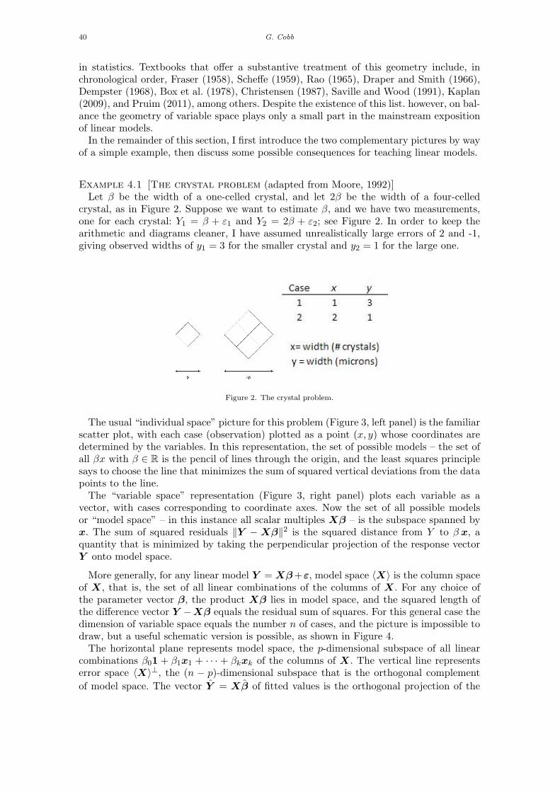
Example 4.1 [The crystal problem (adapted from Moore, 1992)]Let β be the width of a one-celled crystal, and let 2β be the width of a four-celled
crystal, as in Figure 2. Suppose we want to estimate β, and we have two measurements,one for each crystal: Y1 = β + ε1 and Y2 = 2β + ε2; see Figure 2. In order to keep thearithmetic and diagrams cleaner, I have assumed unrealistically large errors of 2 and -1,giving observed widths of y1 = 3 for the smaller crystal and y2 = 1 for the large one.
Figure 2. The crystal problem.
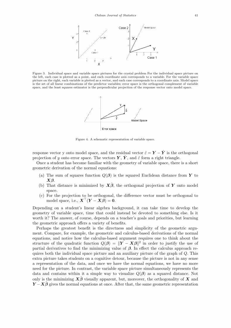
The usual “individual space” picture for this problem (Figure 3, left panel) is the familiarscatter plot, with each case (observation) plotted as a point (x, y) whose coordinates aredetermined by the variables. In this representation, the set of possible models – the set ofall βx with β ∈ R is the pencil of lines through the origin, and the least squares principlesays to choose the line that minimizes the sum of squared vertical deviations from the datapoints to the line.The “variable space” representation (Figure 3, right panel) plots each variable as a
vector, with cases corresponding to coordinate axes. Now the set of all possible modelsor “model space” – in this instance all scalar multiples Xβ – is the subspace spanned byx. The sum of squared residuals ∥Y − Xβ∥2 is the squared distance from Y to β x, aquantity that is minimized by taking the perpendicular projection of the response vectorY onto model space.
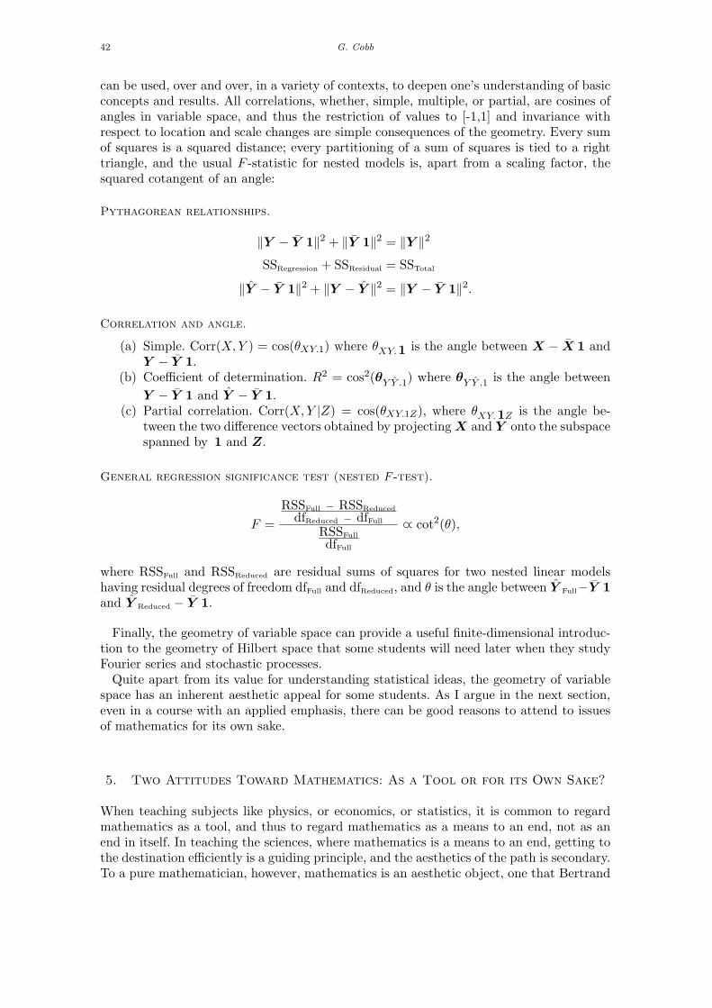
More generally, for any linear model Y = Xβ+ε, model space ⟨X⟩ is the column spaceof X, that is, the set of all linear combinations of the columns of X. For any choice ofthe parameter vector β, the product Xβ lies in model space, and the squared length ofthe difference vector Y −Xβ equals the residual sum of squares. For this general case thedimension of variable space equals the number n of cases, and the picture is impossible todraw, but a useful schematic version is possible, as shown in Figure 4.The horizontal plane represents model space, the p-dimensional subspace of all linear
combinations β01 + β1x1 + · · · + βkxk of the columns of X. The vertical line representserror space ⟨X⟩⊥, the (n − p)-dimensional subspace that is the orthogonal complement
of model space. The vector Y = Xβ of fitted values is the orthogonal projection of the
Chilean Journal of Statistics 41
Figure 3. Individual space and variable space pictures for the crystal problem For the individual space picture onthe left, each case is plotted as a point, and each coordinate axis corresponds to a variable. For the variable spacepicture on the right, each variable is plotted as a vector, and each case corresponds to a coordinate axis. Model spaceis the set of all linear combinations of the predictor variables; error space is the orthogonal complement of variablespace, and the least squares estimator is the perpendicular projection of the response vector onto model space.
Figure 4. A schematic representation of variable space.
response vector y onto model space, and the residual vector ε = Y − Y is the orthogonalprojection of y onto error space. The vectors Y , Y , and ε form a right triangle.Once a student has become familiar with the geometry of variable space, there is a short
geometric derivation of the normal equations:
(a) The sum of squares function Q(β) is the squared Euclidean distance from Y toXβ.
(b) That distance is minimized by Xβ, the orthogonal projection of Y onto modelspace.
(c) For the projection to be orthogonal, the difference vector must be orthogonal tomodel space, i.e., X⊤(Y −Xβ) = 0.
Depending on a student’s linear algebra background, it can take time to develop thegeometry of variable space, time that could instead be devoted to something else. Is itworth it? The answer, of course, depends on a teacher’s goals and priorities, but learningthe geometric approach offers a variety of benefits.Perhaps the greatest benefit is the directness and simplicity of the geometric argu-
ment. Compare, for example, the geometric and calculus-based derivations of the normalequations, and notice how the calculus-based argument requires one to think about thestructure of the quadratic function Q(β) = ∥Y − Xβ∥2 in order to justify the use ofpartial derivatives to find the minimizing value of β. In effect the calculus approach re-quires both the individual space picture and an auxiliary picture of the graph of Q. Thisextra picture takes students on a cognitive detour, because the picture is not in any sensea representation of the data, and once we have the normal equations, we have no moreneed for the picture. In contrast, the variable space picture simultaneously represents thedata and contains within it a simple way to visualize Q(β) as a squared distance. Not
only is the minimizing Xβ visually apparent, but, moreover, the orthogonality of X andY −Xβ gives the normal equations at once. After that, the same geometric representation
42 G. Cobb
can be used, over and over, in a variety of contexts, to deepen one’s understanding of basicconcepts and results. All correlations, whether, simple, multiple, or partial, are cosines ofangles in variable space, and thus the restriction of values to [-1,1] and invariance withrespect to location and scale changes are simple consequences of the geometry. Every sumof squares is a squared distance; every partitioning of a sum of squares is tied to a righttriangle, and the usual F -statistic for nested models is, apart from a scaling factor, thesquared cotangent of an angle:
Pythagorean relationships.
∥Y − Y 1∥2 + ∥Y 1∥2 = ∥Y ∥2
SSRegression + SSResidual = SSTotal
∥Y − Y 1∥2 + ∥Y − Y ∥2 = ∥Y − Y 1∥2.
Correlation and angle.
(a) Simple. Corr(X,Y ) = cos(θXY.1) where θXY.1 is the angle between X − X 1 andY − Y 1.
(b) Coefficient of determination. R2 = cos2(θY Y .1) where θY Y .1 is the angle between
Y − Y 1 and Y − Y 1.(c) Partial correlation. Corr(X,Y |Z) = cos(θXY.1Z), where θXY.1Z is the angle be-
tween the two difference vectors obtained by projectingX and Y onto the subspacespanned by 1 and Z.
General regression significance test (nested F -test).
F =
RSSFull − RSSReduced
dfReduced − dfFullRSSFull
dfFull
∝ cot2(θ),
where RSSFull and RSSReduced are residual sums of squares for two nested linear modelshaving residual degrees of freedom dfFull and dfReduced, and θ is the angle between Y Full−Y 1and Y Reduced − Y 1.
Finally, the geometry of variable space can provide a useful finite-dimensional introduc-tion to the geometry of Hilbert space that some students will need later when they studyFourier series and stochastic processes.Quite apart from its value for understanding statistical ideas, the geometry of variable
space has an inherent aesthetic appeal for some students. As I argue in the next section,even in a course with an applied emphasis, there can be good reasons to attend to issuesof mathematics for its own sake.
5. Two Attitudes Toward Mathematics: As a Tool or for its Own Sake?
When teaching subjects like physics, or economics, or statistics, it is common to regardmathematics as a tool, and thus to regard mathematics as a means to an end, not as anend in itself. In teaching the sciences, where mathematics is a means to an end, getting tothe destination efficiently is a guiding principle, and the aesthetics of the path is secondary.To a pure mathematician, however, mathematics is an aesthetic object, one that Bertrand
Chilean Journal of Statistics 43
Russell compared to sculpture because of the cold austerity of its renunciation of context.Physicists use mathematics to study matter, economists use mathematics to study money,and statisticians use mathematics to study data, but mathematicians themselves boil awaythe applied context, be it matter or money or data, in order to study the clear crystallineresidue of pure pattern. As a former colleague once put it, mathematics is the art form forwhich the medium is the mind.In this section I suggest that even though as statisticians we often and appropriately
regard mathematics as a tool and put a priority on efficiency of derivation and exposition,there are reasons to regard mathematics also as an end in itself, and, at times, to sac-rifice expository efficiency in order to teach in a way that celebrates mathematics as anaesthetic structure. Before presenting an argument, however, it seems useful to be moreconcrete about what I mean by the aesthetic aspects of mathematics, and how teachingwith mathematics as an end in itself differs from teaching with mathematics as a meansto an end.I don’t have anywhere near the qualifications (or for that matter, the patience) to at-
tempt an aesthetic analysis that would be worthy of a philosopher. Instead, I shall focuson just one important feature that to me helps distinguish the mathematical aesthetic,namely, surprise connections revealed by abstract understanding. Over and over in mathe-matics, things that seem completely different on the surface turn out, when understood attheir natural level of generality, to be variations on a common theme. As just one example,consider the way an abstract formulation of the EM algorithm by Dempster et al. (1977)brought a sudden and clarifying unity to a vast array of applied problems and methods.The corresponding experience of revelation – literally a drawing back of the veil – thatsuddenly illuminates, after one has, at last and through effort, achieved an abstract un-derstanding – can strike with all the sudden power of lightening. But just as the dischargein an electrical storm requires preparation through a gradual buildup of positive and neg-ative poles, teaching for aesthetic effect takes time, because students cannot experience asurprise connection between A and B unless they have first come to understand each of Aand B as separate and distinct. Hence the tension between efficiency and aesthetic.For a caricature analog, imagine the choice between a gourmet meal at a fancy restau-
rant and a continuous IV drip of essential nutrients. The IV drip gets the necessary jobdone, with minimal claims on time and attention, but flavor and presentation are equallyminimal.A course about linear models offers many opportunities for surprise connections, al-
though each such opportunity must be paid for with a nominal loss of efficiency. Example5.1 offers a half-dozen instances. Each offers the possibility of a surprise connection betweenan (i) and a (ii). For each, the (i) is a standard element of the mainstream curriculum, andalways taught. The (ii) is typically regarded as optional, sometimes taught, sometimes not.When it is taught, however, it is typically presented as an auxiliary consequence of (i). Inorder to teach the connection between (i) and (ii) as a surprise, it would be necessary topresent (ii) independently and de novo, a choice that would ordinarily be declined as anunaffordable luxury.
Example 5.1 [Six possible surprise connections]
Least squares and projections. (i) Least squares estimators minimize the sum ofsquared residuals – the vertical distances from observed to fitted – and are found bysetting derivatives to zero. (ii) The residual sum of squares is the squared distance fromthe response vector to the column space of the covariates; the least squares estimate isobtained by perpendicular projection.
44 G. Cobb
Correlation and angle. (i) The correlation measures the goodness of (linear) fit. Invari-ance criteria dictate that the squared correlation is a suitably normalized residual sum ofsquares. (ii) The correlation is the cosine of the angle between the mean-adjusted responseand covariate vectors.
Covariance and inner product. (i) When moments exist, the covariance is the integralof the product of the mean-adjusted response and covariate. (ii) If the usual momentassumptions hold (see Section 6), the covariance of two linear combinations is proportionalto the usual Euclidean inner product of their coefficient vectors.
Least squares and Gauss-Markov estimation (i) Least squares estimators have mini-mum variance among linear unbiased estimators, with an algebraic proof. (ii) The linearunbiased estimators constitute a flat set; the estimator with minimum variance correspondsto the shortest coefficient vector in the flat set, which, like the least squares estimator, isobtained by orthogonal projection; see details in Section 8.
The multivariate normal density and the Herschel-Maxwell theorem (see detailsin Section 9) (i) The multivariate normal has density proportional to
exp
(− [Y − µ]⊤Σ−1[Y − µ]
2
).
The chi-square, t and F distributions are defined by their densities, and their relation-ships to the multinormal are derived by calculus. Calculus is also used to show that themultinormal is spherically symmetric, and that orthogonal components are independent.Standard results of sampling theory are derived by calculus. (ii) Given spherical symmetryand the orthogonality property which together define the normal, and given definitions ofchi-square, t and F in terms of the multivariate unit normal, the sampling theory resultscan be derived without relying on densities.
The nested F -test and angle. (i) Given a full model Y = β0x0+β1x1+ε and a reducedmodel Y = β0x0 + ε, a test of the null hypothesis that the reduced model holds can bebased on the F -ratio comparing the two residual sums of squares, as described in Section 4.(ii) Alternatively, a test can be based on the angle between the projections of the responsevector onto the full and reduced model spaces.
With these examples as background, the argument for presenting the theory and practiceof linear models in a way that celebrates their mathematical beauty is straightforward:The continued health and growth of our profession depends on attracting mathematicallytalented students who can rise to the methodological challenges and provide the unifyingabstractions of the future. Many of these students we most need, especially the mostmathematically talented, are attracted to mathematics for its own sake. If we presentstatistics as nothing more than applied data analysis, we may lose them to other subjects.In this context, and in passing, it is worth noticing another tension: Applied data anal-
ysis, because it is anchored in context, tends to pull our profession apart, in opposingdirections. If you choose to analyze data related to marketing, and I choose to analyzedata from molecular biology, the more you and I devote ourselves to our separate areas ofapplication, the less we have in common. In contrast to applied context, our profession’smathematical core is one of the things that hold us together. Even if you choose to domarket research and I choose to work with microarrays, we both may well use generalizedlinear models or hierarchical Bayes. Prior to either of those, we both need a course in linearstatistical models.
Chilean Journal of Statistics 45
This section and the one before it might be seen as an argument for moving our teachingback toward mathematics, and so away from analyzing data, but that is not my intent. Myconviction is that we can recognize the tension between data analysis and mathematics forits own sake without sacrificing one to the other. We can hope that our more mathemati-
cally talented students will aspire to be like the 19th century pioneers Legendre and Gauss,who cared about solving scientific problems and cared about pure mathematics. Statisti-cians know Legendre and Gauss for their work with least squares; pure mathematiciansknow them for their work in number theory.
6. Two Organizing Principles for the Topics in a Course on LinearModels
Like Leo Tolstoy’s happy families, almost all expositions of least squares follow the samegeneral organization, according to the number of covariates in the model: Start with simplelinear regression (one covariate), then move on to a treatment of models with two covari-ates, and from there to models with more than two covariates. (Some treatments skip themiddle stage, and go directly from one covariate to two or more.) This organization-by-dimension echoes the way we traditionally order the teaching of calculus, first spendingtwo semesters on functions of a single variable, and only then turning to functions of twoor more variables.Starting with simple linear regression (and one-variable calculus) offers the very major
advantage that there are exactly as many variables in the model (one response plus onecovariate) are there are dimensions to a blackboard or sheet of paper, which makes itcomparatively easy to draw useful pictures. With two covariates, you need three dimen-sions, and pictures require perspective representations in the plane. With three or morecovariates, you need to rely on training your mind’s eye. A course organized by numberof covariates fits well with the escalating difficulty of visualization; see Kleinbaum andKupper (1978).Despite the very real advantage based on visualization, I conjecture that the main reason
for the near-universality of the usual organization-by-dimension comes from our prerequi-site structure. We take it for granted that students in a least squares course have taken(and indeed, we assume, should have taken) at least one previous course in statistics. Suchstudents will have seen simple linear regression already, so in accordance with an “over-lap principle”, it is sound pedagogy to start the least squares course with something thatoverlaps with what is already at least partially familiar. In short: If we assume studentsalready know about simple linear regression, it makes sense to start their new course withsimple linear regression.Suppose, however, that your students have taken linear algebra, but have never taken
probability or statistics before. Is the usual organization the best choice for these students?As context for thinking about this question, Figure 5 below shows a sense in which thecontent of a least squares course has a natural two-way structure.
Figure 5. Two way structure of the content of a least squares course.
46 G. Cobb
The rows of Figure 5 correspond to three different versions of the linear model:
(a) No distributional assumptions: Y = Xβ + ε, with no assumptions about ε.(b) Moment assumptions Y = Xβ + ε, with E[ε] = 0 and Var[ε] = σ2I, that is, (a)
E[εi] = 0, (b) Var[εi] = σ2, (c) Corr(εi, εj) = 0 if i = j.(c) Normality assumption: Y ∼ Nn(Xβ, σ2I), that is, Y = Xβ + ε, with E[ε]=
0,Var[ε] = σ2I, and each εi is normally distributed.
In the context of Figure 5, the standard organization for a least squares course is “onecolumn at a time”. (i) Start with simple linear regression, and move down the column.First, find the formula for the least squares slope and intercept. Then find the samplingdistribution of the estimators, and use those for confidence intervals and tests. (ii) Havingthus completed the left-most column, move to the middle column and repeat the process:estimators, sampling distributions, intervals and tests. (iii) At some point it is common tomake a transition to matrix notation in order to allow a more compact treatment of thegeneral case. This rough outline offers some flexibility about where to locate additionaltopics such as residual plots, transformations, influence, and multicollinearity, and differentauthors have different preferences, but the general reliance on this outline is near-universal.An alternative organization for a linear models course is “one row at a time”. (i) Start
with no assumptions other than the linearity of the model and the fact that errors areadditive. With no more than this it is possible to fit linear models to a whole range of datasets, with an emphasis on choosing models that offer a reasonable fit to data and context,as in Example 2.1. All four of the methodological challenges described in Example 2.2 canbe addressed in this first part of a course. (ii) Next, add the moment assumptions. Thereare three main theoretical consequences: The moments of the least squares estimators, theexpectation for the mean square error, and the Gauss-Markov theorem, discussed at lengthin Section 8. (iii) Finally, add the assumption that errors are Gaussian. At this point itbecomes possible to obtain the usual sampling distributions, and to use those distributionsfor inference.I see five important advantages to organizing a least squares course by strength of as-
sumptions.
(a) Organizing by assumption follows history, taking what Toeplitz (1963) advocatedas the “genetic” approach to curriculum. For least squares, the earliest work wasdistribution free. The moment and normality assumptions came later, after theleast squares principle and solutions had taken root. As Toeplitz argues, often(though not automatically) what comes earlier in history is easier for students tolearn.
(b) A course organized this way follows a “convergence principle”, beginning from theleast restrictive assumptions and most broadly applicable consequences, then nar-rowing in stages to the most restrictive assumptions and most narrowly applicableconsequences.
(c) This organization gives students an immediate entree to the challenge of modelchoosing. Good applied work in statistics almost always involves the creative pro-cess of choosing a good model, a process that is hard to teach within the narrowconfines of simple linear regression, a context where the only y and x are bothgiven. Put differently, starting with simple linear regression risks coming off as“spinach first, cake after” because the traditional ordering tends to emphasize themechanical and technically difficult, postponing what is most interesting about an-alyzing data until much later in the course. Allowing multiple covariates from thestart gives students an early taste of “the good stuff.”
Chilean Journal of Statistics 47
(d) Organizing by assumptions means that the first part of the course uses no prob-ability, and involves no inference. For several weeks, the course can focus on thecreative challenge of choosing models that offer a good fit to data and a meaningfulconnection to context, without the technical distractions of distributions, p-values,and coverage probabilities.
(e) Finally, and certainly not least, the organization reinforces the important logicalconnection between what you assume and what consequences follow. To the extentthat we want to help our students learn to solve methodological problems, we oweit to them to make clear how what you assume determines what you can conclude.
As I see it, these advantages are relevant for any least squares course, but focus for themoment on the mathematics student who has taken matrix algebra but has not yet takenprobability or statistics. For such a student, the algebraic aspect of working with severalsimultaneous variables is familiar ground. The more fortunate student may even be ac-quainted with the geometry of several dimensions. Probability and statistics, however, arenew, and as experienced teachers know, probability is hard. For students new to the sub-ject, being expected to learn all at once, at the start of a course, about continuous densities,probabilities as areas under curves, expected values and variances both as integrals and asmeasures of long-run behavior, not to mention the initially counter-intuitive post-dictive5
use of probabilities for hypothesis testing – this is a lot to ask, even in the limited contextof simple linear regression. Organizing a least squares course by assumptions introducesprobability only after several weeks of working with linear models.Moreover, probability is introduced in two stages, starting with moments only. By de-
ferring sampling distributions and inference, the “moments-only” section of the course isable to focus on the difficult cognitive challenge of integrating the abstract mathematicaldescription with an intuitive understanding of random behavior and the long run. Sincemoments can be understood as long-run averages, a “moments-only” section offers a gen-tler introduction to probability than does one that covers moments, sampling distributions,and inference all at once.For the third part of the course, the basic results are pretty much standard: inference
about βj , inference about σ2, and the F -test for comparing two nested models. Somecourses may prefer to state and illustrate the results without deriving them, and amongthe many books that do present derivations, there is a variety of approaches. Some authorswork directly with multivariate densities. Others (see, e.g., Hocking, 1996, Chapter 2) relyinstead on moment generating functions. Toward the end of the next section, I describeyet a third approach, based on the Herschel-Maxwell theorem.The next section provides more detail about a possible least squares course organized
by assumptions.
7. One Model or Three?
The organization by assumptions described in the last section amounts to teaching linearmodels as a hierarchy of three classes of models based on assumptions about errors: none,moments only, and the normal distribution for errors. A common alternative is to workwith a single class of models, those for which the conditional distribution of Y given X isnormal with mean Xβ and variance σ2I. Some books (see e.g. Ramsey and Schafer, 2002,p. 180) list all four assumptions of the model simultaneously. Draper and Smith (1966),on the other hand, is explicit that the assumptions need not come as a package. The first16 pages of the book make no assumptions about errors. Then, on p. 17, the moment and
5Dempster (1971) distinguishes between the ordinary, predictive, use of probability and its retrospective, backward-looking, “postdictive” use to assess a model in the context of observed data.
48 G. Cobb
normality assumptions are presented together for the one-predictor case. When the multi-variable case is presented on p. 58, the moment and normality assumptions are included aspart of a single package description of the model. The three kinds of estimation (minimizingthe sum of squared residuals, minimizing the variance among linear unbiased estimators,maximizing the likelihood of the data) are clearly distinguished, but presented one afterthe other in the space of just two pages.Other books (see e.g. Casella and Berger, 2002; Christensen, 1987; Searle, 1971; Ter-
rell, 1999), whose emphasis is more mathematical, are clear and explicit that there arethree models that correspond to three sets of increasingly strong assumptions and threecorresponding sets of consequences, but, sadly in my opinion, books that emphasize dataanalysis tend not to be clear that there are three distinct sets of assumptions, while booksthat are explicit about the hierarchy of assumptions tend not to devote much time andspace to modeling issues, in particular, to the connection between the applied context andthe appropriate set of assumptions.The question, “One model or three?” might be rephrased as a question about the ori-
gins of linear models, in the form “Least squares or regression?” As Stigler (1990) explainsin detail, there are two different origins, separated by almost a century. The later of thetwo origins is cited by one of our best known expositions of linear models, (Neter et al.,1989, p. 26): “Regression was first developed by Sir Francis Galton in the latter part of
the 19th century”. Some books, whether elementary (Freedman et al., 1978) or interme-diate (Ramsey and Schafer, 2002), introduce regression models by means of conditionaldistributions of Y given X. Either, as with Galton, Y and X are assumed to have a jointbivariate normal distribution (see e.g. Freedman et al., 1978), or else the distribution ofX is not specified but the conditional distribution of Y given X is Gaussian (see e.g.,Ramsey and Schafer, 2002). For this approach, there is essentially one model, namely, thatY |X ∼ Nn(Xβ, σ2I).Least squares, in its earliest uses, began about a century earlier than Galton’s work
with the bivariate normal (Stigler, 1990), in a context where the methodological challengewas to find a “solution” to an inconsistent linear system of equations. In the context ofthe astronomical and geodesic challenges in the second half of the 1700s, there was noperceived need, and no recognized basis, for distributional assumptions. The least squaressolution evolved, and then became established, long before Galton. Historically, then, wehad linear models and least squares before, and independently of, any assumptions aboutthe behavior of the errors of observation.Because I have been unable to find a book on least squares whose organization follows
the alternative path I have described, I will spell out in more detail the kind of organizationI use in my own course on linear models. The course has three parts, of roughly six, three,and three weeks each (leaving a week for the inevitable slippage).
Part A [Linearity of the model, additivity of the errors: Y = Xβ + ε] For a courseorganized according to assumptions, the first part takes the deliberately naive view of data,that “what you see is all there is”, i.e., there is no hidden “correct model” to be discovered,no unknown “true parameter values” to be estimated. The goal of the analysis is to find anequation that summarizes the pattern relating y values to x values, an equation that givesa good numerical and graphical fit to the data and good interpretive fit to the appliedcontext, without being needlessly complicated.The essential content for this part of a course has already been described in Section 2
in the context of the AAUP data of Example 2.1. There are four main clusters of topics,each driven by a methodological challenge: (i) Solving inconsistent linear systems; findingleast squares estimates and the geometry of variable space; (ii) measuring goodness of fitand strength of linear relationships; simple, multiple, and partial correlation; adjusting for
Chilean Journal of Statistics 49
a variable and partial residual plots; (iii) measuring influence and properties of the hatmatrix; and (iv) measuring collinearity and the variance inflation factor.As argued in Section 6, the pedagogical advantage of waiting to introduce probability is
that you are thus able to focus in the first several weeks exclusively on issues of modeling,assessing fit, adjusting one set of variables for another set, and the influence of individualcases.
Part B [The moment assumptions: E[εi] = 0, Var[εi] = σ2, Corr(εi, εj) = 0 if i = j] Thethree Moment Assumptions are a Trojan Horse of sorts: Hiding behind an innocent-seemingouter technical shell of probabilistic statements, these assumptions smuggle into our modelthe very strong implied assertion that, apart from random error and modulo the Boxcaveat,6 the response we observe is in fact a true value whose exact functional relationshipto the predictors is indeed known. To me, it is important to do all we can to impress uponour students how hard it should be to take these assumptions at face value.Mathematically, the three main consequences of the moment assumptions are the
moment theorem, that least squares estimators are unbiased with covariance matrixσ2(X⊤X)−1, the variance estimation theorem, that the expected residual mean square isσ2, and the Gauss-Markov theorem, that among linear unbiased estimators, least squaresestimators are best in the sense of having smallest variance. The first two theorems aredirect, matrix-algebraic corollaries of the moment properties of linear combinations ofvectors of independent random variables with mean 0, variance 1.
Proposition Let Z = (Z1, . . . , Zn)⊤ satisfy E[Zi] = 0, Var[Zi] = 1, Corr(Zi, Zj) = 0 if
i = j, a, b ∈ Rn be vectors of constants and c a scalar constant. Then E[a⊤Z + c] = c,Var[a⊤Z + c] = ∥a∥2, and Cov(a⊤Z, b⊤Z) = a · b.
Corollary [Moment theorem] For a linear model that satisfies the Moment Assump-tions, E[β] = β and Var[β] = σ2(X⊤X)−1.
The proof is just a matter of applying the proposition to βj = µ⊤j (X
⊤X)−1X⊤Y , whereµj is a vector of zeros except for a 1 in the jth position.
Proposition Let Z be as above, and A an n×n matrix of constants. Then, E[Z⊤AZ] =σ2tr(A).
Corollary [Variance estimation theorem] E[Y ⊤[I −H]Y ] = σ2(n− p), where p is therank of the hat matrix H = (X⊤X)−1X⊤.
The Gauss-Markov theorem, that least squares estimators are best among linear unbiasedestimators, is typically given short shrift, if it gets any attention at all, but in my opinionthis important result deserves much more attention than it ever gets. Accordingly, I havegiven it in this article a section unto itself, Section 8.
Part C [The normality assumption: the εi are normally distributed] Whereas themoment assumptions specify a long-run relationship between observed values and an un-derlying (assumed) truth, and represent a major step up from the distribution-less model,adding the third layer, that distributions are Gaussian, is a comparatively minor escala-tion, for the usual two reasons: theory guarantees normality when samples are sufficientlylarge; and experience testifies that a suitable transformation can make many unimodaldistributions close to normal. In short, if you’ve got the first two moments, normality canbe just a matter of transformation and possibly a little more data.
6Essentially, all models are wrong; some are useful; see Box and Draper (1987, p. 424).
50 G. Cobb
Although from a practical point of view, going from Part B to Part C is not a big step, Isuggest that nevertheless, there are important pedagogical and curricular reasons to teachParts B and C as very distinct and separate units.The pedagogical reason for working first with just moments, and only later to tackle
entire distributions, was addressed in Section 6: this organization allows a course to focuson how means and variances of linear combinations are tied both to long-run averages andto the geometry of variable space.The main curricular reason to teach “moments first, distributions after” is, as all along,
to highlight the connection between assumptions and consequences. Our third set of as-sumptions – that distributions are normal – allows us to assign probabilities to outcomes.From a practical standpoint, going from moment assumptions to normality is but one smallstep, but from a theoretical standpoint, it is a giant leap. If we can assign probabilities tooutcomes, we can do three very important new things: we can choose estimates that max-imize the postdictive probability of the data; we can use models to assign p-values to tailareas, and use these p-values to compare models; and we can associate a probabilistically-calibrated margin of error with each estimator. In short, the normality assumption opensthe door to maximum likelihood estimation, hypothesis testing, and confidence intervals,none of which are possible if all we have are the first two moments.This section, and the one before it, have presented some reasons to reconsider the way
we organize our exposition of linear models. The next two sections raise questions that areindependent of whether a course is organized by dimension or by assumptions: How muchattention does the Gauss-Markov theorem deserve? How should we teach the samplingdistribution theory we need for inference?
8. The Role of the Gauss-Markov Theorem
In compact acronymic form, the Gauss Markov theorem says that OLS = BLUE: theordinary least squares estimator is best (minimum variance) within the class of linearunbiased estimators. In my opinion, the Gauss-Markov theorem offers a litmus test ofsorts, a useful thought experiment for clarifying course goals and priorities. How muchtime does the result deserve in your treatment of least squares? Among books with anapplied emphasis, most don’t mention Gauss-Markov at all. Some books just state theresult; a few state the theorem and give a quick algebraic proof, of the sort illustrated laterin this section. No book that I am aware of, certainly no book suitable for a first course instatistics, devotes much time and space to the result, although, as I hope to persuade you,a geometric proof can offer students a deeper understanding of the remarkable connectionsamong Euclidean geometry, statistics, and probability.As I see it, a risk in presenting the Gauss-Markov theorem too quickly is that students
will see the result as merely asserting a secondary property of least squares estimators,namely, that their variances have the nice feature of being as small as possible. Whatis at risk of getting lost is that there are two quite different sets of assumptions aboutdata, each with its own approach to estimation. Assuming nothing more than linearity ofthe model with additive errors, we get least squares estimation as a method for solvinginconsistent linear systems. Adding a set of very strong and restrictive assumptions abouterrors opens up an entirely different approach to estimation, starting from the infinite setof all unbiased linear estimators, then choosing the one(s) that minimize variance. On thesurface, there is no reason to expect that the two approaches will always give the sameestimators, and yet they do.
Chilean Journal of Statistics 51
To me, the implication for teaching is clear. To motivate students to appreciate theimportance of the Gauss-Markov theorem, we have to convince them, through concreteexamples, that best linear unbiased estimation is in fact based on a logic very differentfrom that of least squares. Using that logic to obtain Gauss-Markov estimators for specificexamples is an effective way to emphasize the difference. Least squares is purely a methodfor resolving inconsistent linear systems, a method that makes no assumptions whateverabout the behavior of errors apart from their additivity. Gauss-Markov estimation restson very strong assumptions: For every observed value, there is an unobserved, unknowntrue value, and the differences between the observed and true values are random anduncorrelated, with mean zero, and constant SD.These are such strong assumptions that it is not hard to persuade students that for such
a very high price, we should get something better than mere least squares in return. Soour class devotes half a week to finding best linear unbiased estimators, for a variety ofsimple, concrete examples, only to find that we always end up with estimators that arethe same as the least squares estimators. Temporarily at least, the denouement shouldbe a let-down: On the surface, our strong additional assumptions seem to buy us zero!However, on reflection, we can see the result as a surprise endorsement of least squares,in that the assumptions guarantee, via the moment theorem7 that over the long run, leastsquares estimates average out to the true values, provided the model is correct.
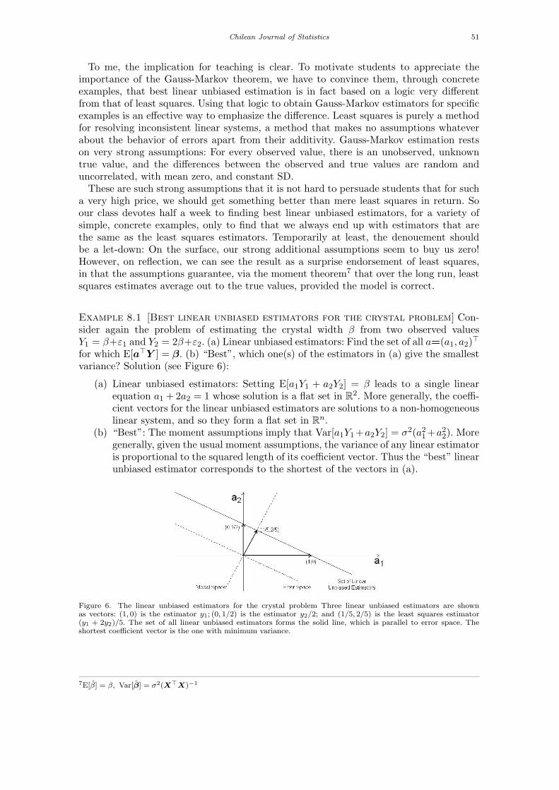
Example 8.1 [Best linear unbiased estimators for the crystal problem] Con-sider again the problem of estimating the crystal width β from two observed valuesY1 = β+ε1 and Y2 = 2β+ε2. (a) Linear unbiased estimators: Find the set of all a=(a1, a2)
⊤
for which E[a⊤Y ] = β. (b) “Best”, which one(s) of the estimators in (a) give the smallestvariance? Solution (see Figure 6):
(a) Linear unbiased estimators: Setting E[a1Y1 + a2Y2] = β leads to a single linearequation a1 +2a2 = 1 whose solution is a flat set in R2. More generally, the coeffi-cient vectors for the linear unbiased estimators are solutions to a non-homogeneouslinear system, and so they form a flat set in Rn.
(b) “Best”: The moment assumptions imply that Var[a1Y1+a2Y2] = σ2(a21+a22). Moregenerally, given the usual moment assumptions, the variance of any linear estimatoris proportional to the squared length of its coefficient vector. Thus the “best” linearunbiased estimator corresponds to the shortest of the vectors in (a).
Figure 6. The linear unbiased estimators for the crystal problem Three linear unbiased estimators are shownas vectors: (1, 0) is the estimator y1; (0, 1/2) is the estimator y2/2; and (1/5, 2/5) is the least squares estimator(y1 + 2y2)/5. The set of all linear unbiased estimators forms the solid line, which is parallel to error space. Theshortest coefficient vector is the one with minimum variance.
7E[β] = β, Var[β] = σ2(X⊤X)−1
52 G. Cobb
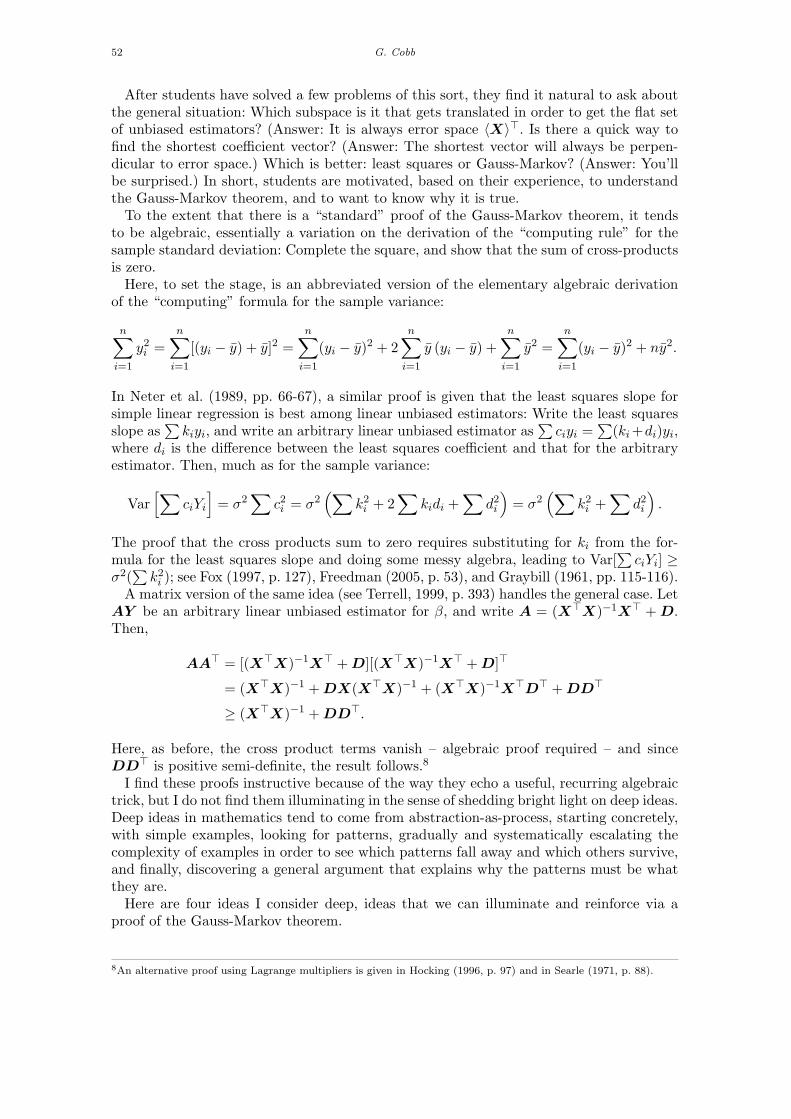
After students have solved a few problems of this sort, they find it natural to ask aboutthe general situation: Which subspace is it that gets translated in order to get the flat setof unbiased estimators? (Answer: It is always error space ⟨X⟩⊤. Is there a quick way tofind the shortest coefficient vector? (Answer: The shortest vector will always be perpen-dicular to error space.) Which is better: least squares or Gauss-Markov? (Answer: You’llbe surprised.) In short, students are motivated, based on their experience, to understandthe Gauss-Markov theorem, and to want to know why it is true.To the extent that there is a “standard” proof of the Gauss-Markov theorem, it tends
to be algebraic, essentially a variation on the derivation of the “computing rule” for thesample standard deviation: Complete the square, and show that the sum of cross-productsis zero.Here, to set the stage, is an abbreviated version of the elementary algebraic derivation
of the “computing” formula for the sample variance:
n∑i=1
y2i =
n∑i=1
[(yi − y) + y]2 =
n∑i=1
(yi − y)2 + 2
n∑i=1
y (yi − y) +
n∑i=1
y2 =
n∑i=1
(yi − y)2 + ny2.
In Neter et al. (1989, pp. 66-67), a similar proof is given that the least squares slope forsimple linear regression is best among linear unbiased estimators: Write the least squaresslope as
∑kiyi, and write an arbitrary linear unbiased estimator as
∑ciyi =
∑(ki+di)yi,
where di is the difference between the least squares coefficient and that for the arbitraryestimator. Then, much as for the sample variance:
Var[∑
ciYi
]= σ2
∑c2i = σ2
(∑k2i + 2
∑kidi +
∑d2i
)= σ2
(∑k2i +
∑d2i
).
The proof that the cross products sum to zero requires substituting for ki from the for-mula for the least squares slope and doing some messy algebra, leading to Var[
∑ciYi] ≥
σ2(∑
k2i ); see Fox (1997, p. 127), Freedman (2005, p. 53), and Graybill (1961, pp. 115-116).A matrix version of the same idea (see Terrell, 1999, p. 393) handles the general case. Let
AY be an arbitrary linear unbiased estimator for β, and write A = (X⊤X)−1X⊤ +D.Then,
AA⊤ = [(X⊤X)−1X⊤ +D][(X⊤X)−1X⊤ +D]⊤
= (X⊤X)−1 +DX(X⊤X)−1 + (X⊤X)−1X⊤D⊤ +DD⊤
≥ (X⊤X)−1 +DD⊤.
Here, as before, the cross product terms vanish – algebraic proof required – and sinceDD⊤ is positive semi-definite, the result follows.8
I find these proofs instructive because of the way they echo a useful, recurring algebraictrick, but I do not find them illuminating in the sense of shedding bright light on deep ideas.Deep ideas in mathematics tend to come from abstraction-as-process, starting concretely,with simple examples, looking for patterns, gradually and systematically escalating thecomplexity of examples in order to see which patterns fall away and which others survive,and finally, discovering a general argument that explains why the patterns must be whatthey are.Here are four ideas I consider deep, ideas that we can illuminate and reinforce via a
proof of the Gauss-Markov theorem.
8An alternative proof using Lagrange multipliers is given in Hocking (1996, p. 97) and in Searle (1971, p. 88).
Chilean Journal of Statistics 53
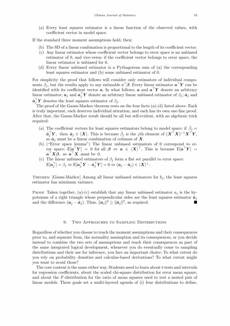
(a) Every least squares estimator is a linear function of the observed values, withcoefficient vector in model space.
If the standard three moment assumptions hold, then:
(b) The SD of a linear combination is proportional to the length of its coefficient vector.(c) Any linear estimator whose coefficient vector belongs to error space is an unbiased
estimator of 0, and vice-versa: if the coefficient vector belongs to error space, thelinear estimator is unbiased for 0.
(d) Every linear unbiased estimator is a Pythagorean sum of (a) the correspondingleast squares estimator and (b) some unbiased estimator of 0.
For simplicity the proof that follows will consider only estimators of individual compo-nents βj , but the results apply to any estimable c⊤β. Every linear estimator a⊤Y can beidentified with its coefficient vector a. In what follows, a and a⊤Y denote an arbitrarylinear estimator; aj and a⊤
j Y denote an arbitrary linear unbiased estimator of βj ; aj and
a⊤j Y denotes the least squares estimator of βj .The proof of the Gauss-Markov theorem rests on the four facts (a)-(d) listed above. Each
is truly important, each deserves individual attention, and each has its own one-line proof.After that, the Gauss-Markov result should be all but self-evident, with no algebraic trickrequired:
(a) The coefficient vectors for least squares estimators belong to model space: if βj =
a⊤j Y , then aj ∈ ⟨X⟩. This is because βj is the jth element of (X⊤X)−1X⊤Y ,
so aj must be a linear combination of columns of X.(b) (“Error space lemma”) The linear unbiased estimators of 0 correspond to er-
ror space: E[a⊤Y ] = 0 for all β ⇔ a ∈ ⟨X⟩⊤. This is because E[a⊤Y ] =a⊤Xβ, so a⊤X must be 0.
(c) The linear unbiased estimators of βj form a flat set parallel to error space:
E[a⊤j ] = βj ⇔ E[a⊤
j Y − a⊤j Y ] = 0 ⇔ (aj − aj) ∈ ⟨X⟩⊥.
Theorem [Gauss-Markov] Among all linear unbiased estimators for bj , the least squaresestimator has minimum variance.
Proof Taken together, (a)-(c) establish that any linear unbiased estimator aj is the hy-potenuse of a right triangle whose perpendicular sides are the least squares estimator aj
and the difference (aj − aj). Thus, ∥aj∥2 ≥ ∥aj∥2, as required. �
9. Two Approaches to Sampling Distributions
Regardless of whether you choose to teach the moment assumptions and their consequencesprior to, and separate from, the normality assumption and its consequences, or you decideinstead to combine the two sets of assumptions and teach their consequences as part ofthe same integrated logical development, whenever you do eventually come to samplingdistributions and their use for inference, you face an important choice: To what extent doyou rely on probability densities and calculus-based derivations? To what extent mightyou want to avoid those?The core content is the same either way. Students need to learn about t-tests and intervals
for regression coefficients, about the scaled chi-square distribution for error mean square,and about the F -distribution for the ratio of mean squares used to test a nested pair oflinear models. These goals set a multi-layered agenda of (i) four distributions to define,
54 G. Cobb
(ii) five basic probabilistic relationships to establish, (iii) three key sampling distributionsto derive (at a minimum), and (iv) the use of those sampling distributions for inference.Four layers of the core agenda for Part C:
(a) Four distributions to define: multivariate normal, chi-square, t, and F .(b) Five probability results:
(b.1) Linear functions of multivariate normals are normal.(b.2) Projections of normals into orthogonal subspaces are independent.(b.3) The squared length of a standard normal vector (mean 0 and variance I) is
chi-square.(b.4) A standard normal divided by the square root of an independent chi-square
is t.(b.5) The ratio of two independent chi-squares over their respective degrees of free-
dom is F .(c) Three essential sampling distributions
(c.1) A studentized regression coefficient has a t distribution.(c.2) The residual sum of squares divided by the true variance is chi-square.(c.3) When the reduced model is true, the F -statistic for comparing full and reduced
models has an F -distribution.(d) Use of the sampling distributions for inference.
At the extremes, I see two competing approaches to the distribution theory. One approach,which for the convenience of having a label, I call “classical”, defines the four distributionsin terms of their probability densities. The five results of the second layer are then derivedusing classical, calculus-based, probability methods. For example, to show (c.1), write theproduct of densities for n unit normals, change to new variables including u = z21+ · · ·+z2n,and integrate over the other variables to obtain the marginal density for u. This result,along with the other four, can then be applied to obtain the three sampling distributionsof the third layer.This “classical” approach sketched above relies heavily on change of variable methods,
multiple integration, and often on generating functions as well. An alternative, which I callhere the “Herschel-Maxwell” approach after the theorem that provides logical justification,makes it possible to avoid calculus entirely. Astronomer Herschel (1850) and physicistMaxwell (1860) are credited with the two-dimensional and three-dimensional versions ofthe theorem that bears their names:9
Theorem [Herschel-Maxwell] Let Z ∈ Rn be a random vector for which (i) projectionsinto orthogonal subspaces are independent and (ii) the distribution of Z depends only onthe length ∥Z∥. Then Z is normally distributed.
If your students are already familiar with multivariate probability densities from a pre-vious probability course, then establishing the converse of the theorem, proving (i) and(ii) above starting from the multivariate normal density, turns out to be easy. However, ifyou are teaching this material – inference for least squares – to students who have not yetseen probability densities, and who may not have seen any multivariable calculus either,the “classical” approach will be a stretch, at best. You can always finesse the distributiontheory as “beyond the scope of this course”, and many good books with an applied empha-sis choose to do just that. But when I am teaching a course for students of mathematics,although I may be willing to omit an occasional proof, I would be embarrassed to presentkey sampling distributions as a set of black boxes.
9See Jaynes (2003, pp. 201-201) for Herschel’s argument for the two-dimensional case, which Maxwell later extendedto three dimensions.
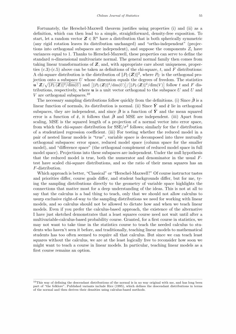
Chilean Journal of Statistics 55
Fortunately, the Herschel-Maxwell theorem justifies using properties (i) and (ii) as adefinition, which can then lead to a simple, straightforward, density-free exposition. Tostart, let a random vector Z ∈ Rn have a distribution that is both spherically symmetric(any rigid rotation leaves its distribution unchanged) and “ortho-independent” (projec-tions into orthogonal subspaces are independent), and suppose the components Zi havevariances equal to 1. Thanks to Herschel-Maxwell, these properties can serve to define thestandard n-dimensional multivariate normal. The general normal family then comes fromtaking linear transformations of Z, and, with appropriate care about uniqueness, proper-ties (c.3)-(c.5) above can be taken as definitions of the chi-square, t, and F distributions:A chi-square distribution is the distribution of ∥PU (Z)∥2, where PU is the orthogonal pro-jection onto a subspace U whose dimension equals the degrees of freedom. The statisticsu⊤Z/
√∥PU (Z)∥2/dim(U) and
[∥PU (Z)∥2/dim(U)
]/[∥PV (Z)∥2/dim(V )
]follow t and F dis-
tributions, respectively, where u is a unit vector orthogonal to the subspace U and U andV are orthogonal subspaces.10
The necessary sampling distributions follow quickly from the definitions. (i) Since β is a
linear function of normals, its distribution is normal. (ii) Since Y and ε lie in orthogonal
subspaces, they are independent, and since β is a function of Y and the mean squarederror is a function of ε, it follows that β and MSE are independent. (iii) Apart fromscaling, MSE is the squared length of a projection of a normal vector into error space,from which the chi-square distribution for SSE/σ2 follows; similarly for the t distributionof a studentized regression coefficient. (iii) For testing whether the reduced model in apair of nested linear models is “true”, variable space is decomposed into three mutuallyorthogonal subspaces: error space, reduced model space (column space for the smallermodel), and “difference space” (the orthogonal complement of reduced model space in fullmodel space). Projections into these subspaces are independent. Under the null hypothesisthat the reduced model is true, both the numerator and denominator in the usual F -test have scaled chi-square distributions, and so the ratio of their mean squares has anF -distribution.Which approach is better, “Classical” or “Herschel-Maxwell?” Of course instructor tastes
and priorities differ, course goals differ, and student backgrounds differ, but for me, ty-ing the sampling distributions directly to the geometry of variable space highlights theconnections that matter most for a deep understanding of the ideas. This is not at all tosay that the calculus is a bad thing to teach, only that we should not allow calculus tousurp exclusive right-of-way to the sampling distributions we need for working with linearmodels, and so calculus should not be allowed to dictate how and when we teach linearmodels. Even if you prefer the calculus-based approach, the existence of the alternativeI have just sketched demonstrates that a least squares course need not wait until after amultivariable-calculus-based probability course. Granted, for a first course in statistics, wemay not want to take time in the statistics course to teach the needed calculus to stu-dents who haven’t seen it before, and traditionally, teaching linear models to mathematicalstudents has too often seemed to require all that calculus. But since we can teach leastsquares without the calculus, we are at the least logically free to reconsider how soon wemight want to teach a course in linear models. In particular, teaching linear models as afirst course remains an option.
10This way of defining the descendant distributions of the normal is in no way original with me, and has long beenpart of “the folklore”. Published variants include Rice (1995), which defines the descendant distributions in termsof the normal and then derives their densities using calculus-based methods.
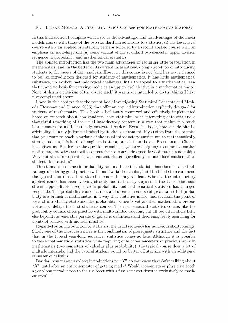
56 G. Cobb
10. Linear Models: A First Statistics Course for Mathematics Majors?
In this final section I compare what I see as the advantages and disadvantages of the linearmodels course with those of the two standard introductions to statistics: (i) the lower levelcourse with a an applied orientation, perhaps followed by a second applied course with anemphasis on modeling, and (ii) some variant of the standard two-semester upper divisionsequence in probability and mathematical statistics.The applied introduction has the two main advantages of requiring little preparation in
mathematics, and, in the better of its current incarnations, doing a good job of introducingstudents to the basics of data analysis. However, this course is not (and has never claimedto be) an introduction designed for students of mathematics. It has little mathematicalsubstance, no explicit methodological challenges, little to appeal to a mathematical aes-thetic, and no basis for carrying credit as an upper-level elective in a mathematics major.None of this is a criticism of the course itself; it was never intended to do the things I havejust complained about.I note in this context that the recent book Investigating Statistical Concepts and Meth-
ods (Rossman and Chance, 2006) does offer an applied introduction explicitly designed forstudents of mathematics. This book is brilliantly conceived and effectively implementedbased on research about how students learn statistics, with interesting data sets and athoughtful reworking of the usual introductory content in a way that makes it a muchbetter match for mathematically motivated readers. Even this book, however, despite itsoriginality, is in my judgment limited by its choice of content. If you start from the premisethat you want to teach a variant of the usual introductory curriculum to mathematicallystrong students, it is hard to imagine a better approach than the one Rossman and Chancehave given us. But for me the question remains: If you are designing a course for mathe-matics majors, why start with content from a course designed for a different readership?Why not start from scratch, with content chosen specifically to introduce mathematicalstudents to statistics?The standard sequence in probability and mathematical statistic has the one salient ad-
vantage of offering good practice with multivariable calculus, but I find little to recommendthe typical course as a first statistics course for any student. Whereas the introductoryapplied course has been evolving steadily and in healthy ways since the 1960s, the mainstream upper division sequence in probability and mathematical statistics has changedvery little. The probability course can be, and often is, a course of great value, but proba-bility is a branch of mathematics in a way that statistics is not, and so, from the point ofview of introducing statistics, the probability course is yet another mathematics prereq-uisite that delays the first statistics course. The mathematical statistics course, like theprobability course, offers practice with multivariable calculus, but all too often offers littleelse beyond its venerable parade of geriatric definitions and theorems, feebly searching forpoints of contact with modern practice.Regarded as an introduction to statistics, the usual sequence has numerous shortcomings.
Surely one of the most restrictive is the combination of prerequisite structure and the factthat in the typical year-long sequence, statistics comes so late. Although it is possibleto teach mathematical statistics while requiring only three semesters of previous work inmathematics (two semesters of calculus plus probability), the typical course does a lot ofmultiple integrals, and the typical student would be better off starting with an additionalsemester of calculus.Besides, how many year-long introductions to “X” do you know that defer talking about
“X” until after an entire semester of getting ready? Would economists or physicists teacha year-long introduction to their subject with a first semester devoted exclusively to math-ematics?
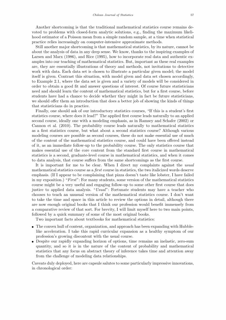
Chilean Journal of Statistics 57
Another shortcoming is that the traditional mathematical statistics course remains de-voted to problems with closed-form analytic solutions, e.g., finding the maximum likeli-hood estimator of a Poisson mean from a simple random sample, at a time when statisticalpractice relies increasingly on computer-intensive approximate methods.Still another major shortcoming is that mathematical statistics, by its nature, cannot be
about the analysis of data in any deep sense. We know, thanks to the inspiring examples ofLarsen and Marx (1986), and Rice (1995), how to incorporate real data and authentic ex-amples into our teaching of mathematical statistics. But, important as these real examplesare, they are essentially illustrations of theory and methods, not invitations to detectivework with data. Each data set is chosen to illustrate a particular given model; the modelitself is given. Contrast this situation, with model given and data set chosen accordingly,to Example 2.1, where the data set is given and a variety of models will be considered inorder to obtain a good fit and answer questions of interest. Of course future statisticiansneed and should learn the content of mathematical statistics, but for a first course, beforestudents have had a chance to decide whether they might in fact be future statisticians,we should offer them an introduction that does a better job of showing the kinds of thingsthat statisticians do in practice.Finally, one should ask of our introductory statistics courses, “If this is a student’s first
statistics course, where does it lead?” The applied first course leads naturally to an appliedsecond course, ideally one with a modeling emphasis, as in Ramsey and Schafer (2002) orCannon et al. (2010). The probability course leads naturally to mathematical statisticsas a first statistics course, but what about a second statistics course? Although variousmodeling courses are possible as second courses, these do not make essential use of muchof the content of the mathematical statistics course, and could have been offered insteadof it, as an immediate follow-up to the probability course. The only statistics course thatmakes essential use of the core content from the standard first course in mathematicalstatistics is a second, graduate-level course in mathematical statistics, and when it comesto data analysis, that course suffers from the same shortcomings as the first course.It is important for me to be clear. When I direct my complaints against the usual
mathematical statistics course as a first course in statistics, the two italicized words deserveemphasis. (If I appear to be complaining that pizza doesn’t taste like lobster, I have failedin my exposition.) “First”: For many students, some version of the mathematical statisticscourse might be a very useful and engaging follow-up to some other first course that doesjustice to applied data analysis. “Usual”: Fortunate students may have a teacher whochooses to teach an unusual version of the mathematical statistics course. I don’t wantto take the time and space in this article to review the options in detail, although thereare now enough original books that I think our profession would benefit immensely froma comparative review of that sort. For brevity, I will limit myself here to two main points,followed by a quick summary of some of the most original books.Two important facts about textbooks for mathematical statistics:
• The convex hull of content, organization, and approach has been expanding with Hubble-like acceleration. I take this rapid curricular expansion as a healthy symptom of ourprofession’s growing discontent with the usual course.
• Despite our rapidly expanding horizon of options, time remains an inelastic, zero-sumquantity, and so it is in the nature of the content of probability and mathematicalstatistics that any focus on abstract theory of inference takes time and attention awayfrom the challenge of modeling data relationships.
Caveats duly deployed, here are capsule salutes to some particularly impressive innovations,in chronological order:
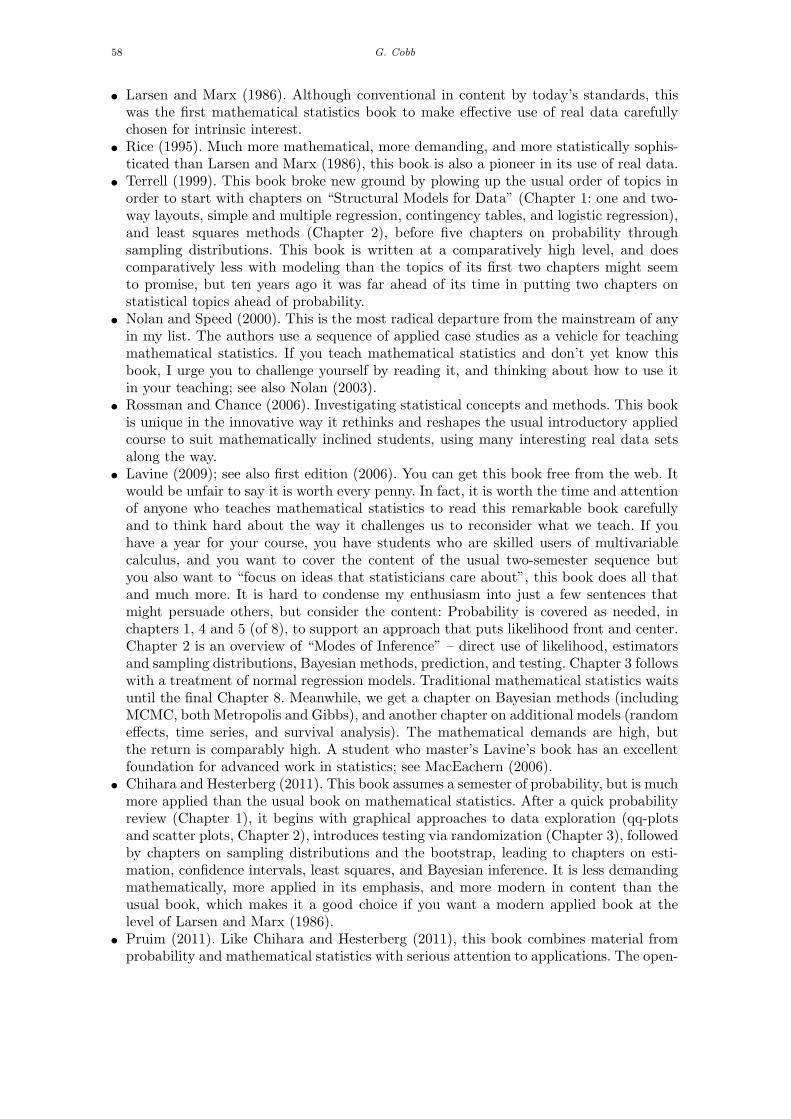
58 G. Cobb
• Larsen and Marx (1986). Although conventional in content by today’s standards, thiswas the first mathematical statistics book to make effective use of real data carefullychosen for intrinsic interest.
• Rice (1995). Much more mathematical, more demanding, and more statistically sophis-ticated than Larsen and Marx (1986), this book is also a pioneer in its use of real data.
• Terrell (1999). This book broke new ground by plowing up the usual order of topics inorder to start with chapters on “Structural Models for Data” (Chapter 1: one and two-way layouts, simple and multiple regression, contingency tables, and logistic regression),and least squares methods (Chapter 2), before five chapters on probability throughsampling distributions. This book is written at a comparatively high level, and doescomparatively less with modeling than the topics of its first two chapters might seemto promise, but ten years ago it was far ahead of its time in putting two chapters onstatistical topics ahead of probability.
• Nolan and Speed (2000). This is the most radical departure from the mainstream of anyin my list. The authors use a sequence of applied case studies as a vehicle for teachingmathematical statistics. If you teach mathematical statistics and don’t yet know thisbook, I urge you to challenge yourself by reading it, and thinking about how to use itin your teaching; see also Nolan (2003).
• Rossman and Chance (2006). Investigating statistical concepts and methods. This bookis unique in the innovative way it rethinks and reshapes the usual introductory appliedcourse to suit mathematically inclined students, using many interesting real data setsalong the way.
• Lavine (2009); see also first edition (2006). You can get this book free from the web. Itwould be unfair to say it is worth every penny. In fact, it is worth the time and attentionof anyone who teaches mathematical statistics to read this remarkable book carefullyand to think hard about the way it challenges us to reconsider what we teach. If youhave a year for your course, you have students who are skilled users of multivariablecalculus, and you want to cover the content of the usual two-semester sequence butyou also want to “focus on ideas that statisticians care about”, this book does all thatand much more. It is hard to condense my enthusiasm into just a few sentences thatmight persuade others, but consider the content: Probability is covered as needed, inchapters 1, 4 and 5 (of 8), to support an approach that puts likelihood front and center.Chapter 2 is an overview of “Modes of Inference” – direct use of likelihood, estimatorsand sampling distributions, Bayesian methods, prediction, and testing. Chapter 3 followswith a treatment of normal regression models. Traditional mathematical statistics waitsuntil the final Chapter 8. Meanwhile, we get a chapter on Bayesian methods (includingMCMC, both Metropolis and Gibbs), and another chapter on additional models (randomeffects, time series, and survival analysis). The mathematical demands are high, butthe return is comparably high. A student who master’s Lavine’s book has an excellentfoundation for advanced work in statistics; see MacEachern (2006).
• Chihara and Hesterberg (2011). This book assumes a semester of probability, but is muchmore applied than the usual book on mathematical statistics. After a quick probabilityreview (Chapter 1), it begins with graphical approaches to data exploration (qq-plotsand scatter plots, Chapter 2), introduces testing via randomization (Chapter 3), followedby chapters on sampling distributions and the bootstrap, leading to chapters on esti-mation, confidence intervals, least squares, and Bayesian inference. It is less demandingmathematically, more applied in its emphasis, and more modern in content than theusual book, which makes it a good choice if you want a modern applied book at thelevel of Larsen and Marx (1986).
• Pruim (2011). Like Chihara and Hesterberg (2011), this book combines material fromprobability and mathematical statistics with serious attention to applications. The open-
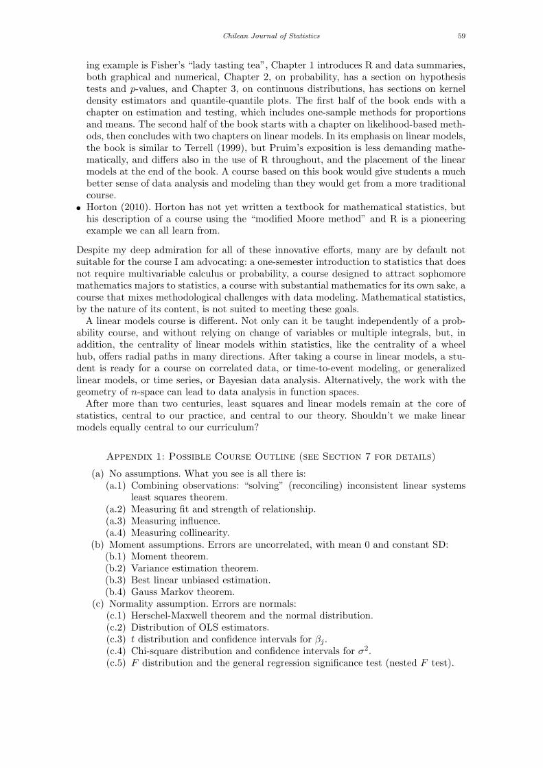
Chilean Journal of Statistics 59
ing example is Fisher’s “lady tasting tea”, Chapter 1 introduces R and data summaries,both graphical and numerical, Chapter 2, on probability, has a section on hypothesistests and p-values, and Chapter 3, on continuous distributions, has sections on kerneldensity estimators and quantile-quantile plots. The first half of the book ends with achapter on estimation and testing, which includes one-sample methods for proportionsand means. The second half of the book starts with a chapter on likelihood-based meth-ods, then concludes with two chapters on linear models. In its emphasis on linear models,the book is similar to Terrell (1999), but Pruim’s exposition is less demanding mathe-matically, and differs also in the use of R throughout, and the placement of the linearmodels at the end of the book. A course based on this book would give students a muchbetter sense of data analysis and modeling than they would get from a more traditionalcourse.
• Horton (2010). Horton has not yet written a textbook for mathematical statistics, buthis description of a course using the “modified Moore method” and R is a pioneeringexample we can all learn from.
Despite my deep admiration for all of these innovative efforts, many are by default notsuitable for the course I am advocating: a one-semester introduction to statistics that doesnot require multivariable calculus or probability, a course designed to attract sophomoremathematics majors to statistics, a course with substantial mathematics for its own sake, acourse that mixes methodological challenges with data modeling. Mathematical statistics,by the nature of its content, is not suited to meeting these goals.A linear models course is different. Not only can it be taught independently of a prob-
ability course, and without relying on change of variables or multiple integrals, but, inaddition, the centrality of linear models within statistics, like the centrality of a wheelhub, offers radial paths in many directions. After taking a course in linear models, a stu-dent is ready for a course on correlated data, or time-to-event modeling, or generalizedlinear models, or time series, or Bayesian data analysis. Alternatively, the work with thegeometry of n-space can lead to data analysis in function spaces.After more than two centuries, least squares and linear models remain at the core of
statistics, central to our practice, and central to our theory. Shouldn’t we make linearmodels equally central to our curriculum?
Appendix 1: Possible Course Outline (see Section 7 for details)
(a) No assumptions. What you see is all there is:(a.1) Combining observations: “solving” (reconciling) inconsistent linear systems
least squares theorem.(a.2) Measuring fit and strength of relationship.(a.3) Measuring influence.(a.4) Measuring collinearity.
(b) Moment assumptions. Errors are uncorrelated, with mean 0 and constant SD:(b.1) Moment theorem.(b.2) Variance estimation theorem.(b.3) Best linear unbiased estimation.(b.4) Gauss Markov theorem.
(c) Normality assumption. Errors are normals:(c.1) Herschel-Maxwell theorem and the normal distribution.(c.2) Distribution of OLS estimators.(c.3) t distribution and confidence intervals for βj .(c.4) Chi-square distribution and confidence intervals for σ2.(c.5) F distribution and the general regression significance test (nested F test).
60 G. Cobb
Appendix 2: AAUP Data (Bellas and Reskin, 1994)
Subject AvAcSal PctFem PctUnemp PctNonAc MedNASalDentistry 44214 15.7 0.1 99.4 40005Medicine 43160 25.5 0.2 96.0 50005Law 40670 34.0 0.5 99.3 30518Agriculture 36879 12.9 0.8 43.4 31063Engineering 35694 4.6 0.5 65.5 35133Geology 33206 13.5 0.3 58.1 33602Chemistry 33069 16.2 1.1 61.9 32489Physics 32925 7.2 1.2 40.7 33434LifeSciences 32605 29.8 1.4 27.4 30500Economics 32179 14.8 0.3 34.2 37052Philosophy 31430 23.1 1.8 17.1 18500History 31276 30.5 1.5 20.5 21113Business 30753 27.1 1.9 98.9 20244Architecture 30337 31.6 1.1 98.3 21758Psychology 29894 45.5 1.1 51.0 30807EducPsych 29675 49.5 0.9 82.5 20195SocialWork 29208 80.0 1.9 98.6 16965Mathematics 29128 15.4 0.4 17.9 32537Education 28952 48.1 0.7 97.1 19465SocAnthro 27633 40.9 2.1 12.8 21600Art 27198 57.6 2.1 96.6 11586Music 26548 45.5 4.3 98.5 16193Journalism 25950 52.3 3.1 93.4 20135English 25892 53.6 1.9 12.1 18000ForeignLang 25566 55.0 3.5 12.1 20352Nursing 24924 94.2 1.4 96.2 17505Drama 24865 58.5 5.5 97.1 20005LibraryScience 23658 82.2 1.1 78.9 15980
Where AvAcSal = mean academic salary; PctFem = percentage of faculty who are women; PctUn= percentage unemployed; PctNonAc = percentage of jobs that are not academic; MedNASal =median non-academic salary.
References
Bartlett, M.S., 1933. The vector representation of a sample. Proceedings of the CambridgePhilosophical Society, 30, 327-340.
Bellas, M., Reskin, B.F., 1994. On comparable worth. Academe, 80, 83-85.Box, G.E.P., Draper, N.R., 1987. Empirical Model-Building and Response Surfaces. John
Wiley & Sons, New York.Box, G.E.P., Hunter, W.G., Hunter, J.S., 1978. Statistics for Experimenters: An Introduc-
tion to Design, Data Analysis, and Model Building. John Wiley & Sons, New York.Breiman, L., 1969. Probability and Stochastic Processes with a View Toward Applications.
Houghton-Mifflin, Boston.Bryant, P., 1984. Geometry, statistics, probability: variations on a common theme. The
American Statistician, 38, 38-48.Cannon, A.R., Cobb, G.W., Hartlaub, B.A., Legler, J.M., Lock, R.H., Moore, T.L., Ross-
man, A.J., Witmer, J.A., 2010. Stat 2: A Second Course in Undergraduate Statistics.Freeman, New York (accepted for publication).
Casella, G., Berger, R.L., 2002. Statistical Inference. 2nd edition. Duxbury, Pacific Grove,California.
Chihara, L., Hesterberg, T., 2011. Mathematical Statistics with Resampling and R. JohnWiley & Sons, New York (to appear).
Chilean Journal of Statistics 61
Christensen, R., 1987. Plane Answers to Complex Questions. Springer-Verlag, New York.Dempster, A.P., 1968. Elements of Continuous Multivariate Analysis. Addison-Wesley,
Reading, Massachusetts.Dempster, A.P., 1971. Model searching and estimation in the logic of inference. In Go-
dambe, V.P., Sprott, D.A., (eds.). Foundations of Statistical Inference, Holt, Rinehartand Winston, Toronto, pp. 56-78.
Dempster, A.P., Laird, N.M., Rubin D.B., 1977. Maximum likelihood from incomplete datavia the EM algorithm. Journal of The Royal Statistical Society Series B - StatisticalMethodology, 39, 1-38.
Draper, N.R., Smith, H., 1966. Applied Regression Analysis. John Wiley & Sons, NewYork.
Eaton, M.L., 2007. William H. Kruskal and the development of Coordinate-Free Methods.Statistical Science, 22, 264-265.
Fox, J., 1997. Applied Regression Analysis, Linear Models, and Related Methods. Sage,Thousand Oaks, California.
Fraser, D.A.S., 1958. Statistics: An Introduction. John Wiley & Sons, New York.Freedman, D.A., 2005. Statistical Models: Theory and Practice. Cambridge University
Press, Cambridge.Freedman, D.A., Pisani, R., Purves, R., 1978. Statistics. Norton, New York.Graybill, F.A., 1961. An Introduction to Linear Statistical Models – Volume 1. McGraw-
Hill, New York.Herschel, J.F.W., 1850. Quetelet on probabilities. Edinburgh and Quarterly Reviews, 92,
1-57.Herr, D.G., 1980. On the history of the use of geometry in the general linear model. The
American Statistician, 34, 43-47.Hoaglin, D.C., Welsch, R.E., 1978. The hat matrix in regression and ANOVA. The Amer-
ican Statistician, 32, 17-22.Hocking, R.R., 1996. Methods and Applications of Linear Models. John Wiley & Sons,
New York.Hoel, P., 1947. Introduction to Mathematical Statistics. John Wiley & Sons, New York.Hogg, R.V., Craig, A.T., 1959. Introduction to Mathematical Statistics. MacMillan, New
York.Horton, N.J., 2010. I Hear, I Forget. I Do, I Understand: Using R as the Centerpiece of a
Modified Moore-Method Mathematical Statistics Course. In progress.Horton, N.J., Brown, E.R., Qian, L., 2004. Use of R as a toolbox for mathematical statistics
exploration. The American Statistician, 58, 343-357.Jaynes, E.T., 2003. Probability Theory: The Logic of Science. Cambridge University Press,
Cambridge.Johnson, R.W., 1994. Estimating the size of a population. Teaching Statistics, 16, 50.Kaplan, D.T., 2009. Statistical Modeling: A Fresh Approach. CreateSpace, Seattle.Kleinbaum, D.G., Kupper, L.L., 1978. Applied Regression Analysis and Other Multivariate
Methods. Duxbury, North Scituate, Massachusetts.Kruskal, W.G., 1961. The coordinate-free approach to Gauss–Markov estimation and its
application to missing and extra observations. Proc. Fourth Berkeley Symposium onMathematical Statististics and Probability. University California Press, Berkeley, pp.435-451.
Kuhn, T.S., 1962. The Structure of Scientific Revolutions. University of Chicago Press,Chicago.
Kuhn, T.S., 1977. The Essential Tension: Selected Studies in Scientific Tradition andChange. University of Chicago Press, Chicago.
62 G. Cobb
Larsen, R.J., Marx, M.L., 1986. An Introduction to Mathematical Statistics and Its Ap-plications. 2nd edition, Prentice-Hall, Englewood Cliffs, New Jersey.
Lavine, M., 2009. Introduction to Statistical Thought. Orange Grove Texts Plus, FL, USA.Available at http://www.math.umass.edu/~lavine/Book/book.html.
MacEachern, S.N., 2006. Review of Introduction to Statistical Thought. A publicationfrom Journal of the American Statistical Association, USA.
Maxwell, J.C., 1860. Illustration of the dynamical theory of gases. Part 1. On the motionsand collisions of perfectly elastic spheres. Philosophical Magazine, 19-32.
Moore, T.L., 1992. Getting more data into theoretical statistics courses. PRIMUS, 2, 348-356.
Neter, J., Wasserman, W., Kutner, M.H., 1989. Applied Linear Regression Models. 2ndedition, Irwin, Homewood, Illinois.
Nolan, D.A., 2003. Case studies in the mathematical statistics course. Science and Statis-tics: A Festschrift for Terry Speed. IMS Press, Fountain Hills, Arizona, pp. 165-176.
Nolan, D., Speed, T., 2000. Stat Labs: Mathematical Statistics through Applications.Springer-Verlag-Verlag, New York.
Olkin, I., Gleser, L.J., Derman, C., 1980. Probability Models and Applications. Macmillan,New York.
Pruim, R., 2011. Foundations and Applications of Statistics. AMS, Providence (to appear).Ramsey, F.L. Schafer, D.W., 2002. The Statistical Sleuth: A Course in Methods of Data
Analysis. 2nd edition, Duxbury, Pacific Grove, California.Rao, C.R., 1965. Linear Statistical Inference and Its Applications. John Wiley & Sons,
New York.Rice, J.A., 1995. Mathematical Statistics and Data Analysis. 2nd edition, Duxbury, Bel-
mont, California.Rossman, A., Chance, B., 2006. Investigating Statistical Concepts and Methods. Duxbury,
Pacific Grove, California.Saville, D.J., Wood, G.R., 1991. Statistical Methods: The Geometric Approach. Springer-
Verlag-Verlag, New York.Scheffe, H., 1959. The Analysis of Variance. John Wiley & Sons, New York.Searle, S.R., 1971. Linear Models. John Wiley & Sons, New York.Stigler, S.M., 1990. The History of Statistics: The Measurement of Uncertainty before
1900. Harvard University Press, Cambridge, Massachusetts.Terrell, G.C., 1999. Mathematical Statistics: A Unified Introduction. Springer-Verlag, New
York.Toeplitz, O., 1963. The Calculus: A Genetic Approach. University of Chicago Press,
Chicago.