Teacher Performance Pay in the United States:Incidence and Adult Outcomes

Timothy N. Bond Kevin J. MumfordPurdue University & IZA Purdue University

March 2018

Abstract

This paper estimates the effect of exposure to teacher pay-for-performance programson adult outcomes. We construct a comprehensive data set of schools which haveimplemented teacher performance pay programs across the United States since 1986,and use our data to calculate the fraction of students by race in each grade and ineach state who are affected by a teacher performance pay program in a given year.We then calculate the expected years of exposure for each race-specific birth state-grade cohort in the American Community Survey. Cohorts with more exposure aremore likely to graduate from high school and earn higher wages as adults. The positiveeffect is concentrated in grades 1-3 and on programs that targeted schools with a higherfraction of students who are eligible for free and reduced lunch.

JEL Codes: I21, J24

Keywords: Teacher Performance Pay; Adult Outcomes

We are grateful to participants at the APPAM Fall Conference, the European Association of LaborEconomists Conference, the ASSA Annual Meeting, and seminar participants at Brigham Young University,Ohio State University, Purdue University, and the University of Nottingham for their helpful comments. Wewould like to thank Mary Kate Batistich, Jacklyn Buhrmann, Kendall Kennedy, Sophie Shen, and WanlingZou for excellent research assistance. Any remaining errors are our own.

I Introduction

Approximately all public school teachers are paid according to a salary schedule that dif-

ferentiates pay by experience, seniority, and credentials, but not generally by observed per-

formance (Podgursky, 2007). Education reformers have long viewed this as problematic for

two reasons. First, the classroom environment presents a classic case of moral hazard: it

is difficult for a principal to observe the collective set of actions taken by a teacher over

the school year and to know what the optimal set of actions would have been (Neal, 2011).

Second, the characteristics that do differentiate pay under the salary schedule have little

correlation with teacher performance (Hanushek, 2003).

As a consequence, and in conjunction with the advent of modern standardized testing,

policy makers have increasingly sought to tie teacher pay to student test performance.1

A comprehensive review of the literature by Neal (2011) finds that when teachers receive

bonuses tied to their own students’ scores on a specific test, their students’ scores on that

test generally increase. But, there are three major reasons to be skeptical of such analyses:

(1) test scores can be manipulated by teaching to the test or by orchestrated cheating, (2)

test scores do not reflect many important skills that can be taught, and (3) test scores are

measured on ordinal scales which makes over-time or across-group comparisons unconvincing.

In this paper, we avoid these concerns by estimating the effect of teacher performance

pay programs on wages and other adult outcomes. We find that one year of exposure to a

teacher performance pay program in the United States leads to an increase in adult wages

of 1.9 percent, a 0.5 percentage point reduction in unemployment, and a 0.6 percentage

point increase in labor force participation. Each year of exposure is estimated to increase

the likelihood of graduation from high school by 1 percentage point. These estimates are

1Tying teacher pay to test scores is only the latest initiative in the long-standing effort to differentiateteacher pay by ability. The previous iteration came through the movement towards “career ladders” in the1980s, which gave higher salaries to teachers who obtained more education, outside credentials, and passedevaluations through classroom observations. These programs were generally deemed overly expensive, withlittle evidence of success on student outcomes, and were almost universally abolished by the early 1990’s(Cornett and Gaines, 1994).

2

obtained from a specification in which we include birth-year-by-state fixed effects which

controls for all other state-specific education reforms that may be correlated with the decision

to implement teacher performance pay.

The literature has focused on estimating the effect on student test scores for specific (gen-

erally state- or city-level) teacher performance-pay programs.2 We have already discussed

the shortcomings of this approach and there is strong empirical evidence to suggest these

concerns are not trivial. Jacob and Levitt (2003) found evidence that teachers responded to

the introduction of high-stakes testing in Chicago by changing student answers, i.e. cheating.

Koretz and Barron (1998) found that the introduction of test-based accountability led to in-

creases in student performance on the test that was used for school evaluations, but not on

tests that were not. Even evaluating performance pay programs with tests that were not used

for bonus schemes can be problematic. Teachers may direct resources to test-taking skills

which have positive effects on all test scores, without any human capital gains (Neal, 2013).

Finally, Bond and Lang (2013) show that estimated effects in the black-white test score

gap literature are not robust to order-preserving scale transformations of test scores. This

implies that the test scale may itself be responsible for some of the differences in estimated

effects across performance pay programs.

Few researchers have attempted to evaluate school policy using adult outcomes rather

than test scores. Chetty, Friedman, and Rockoff (2014) examine the relationship between

teacher quality and adult wages using teacher value-added. Heckman, Pinto, and Savelyev

(2013) use adult outcomes to evaluate the Perry Preschool program. Dobbie and Fryer

(2016) use adult outcomes to evaluate the performance of charter schools. Card and Krueger

(1998) find weak evidence that school resources are positively correlated with adult outcomes,

while Jackson, Johnson, and Persico (2016) estimate that a 10 percent increase in per pupil

2Many studies have found a positive effect on test scores including Cooper and Cohn (1997) in SouthCarolina, Ladd (1999) in Dallas, Dee and Keys (2004) in Tennessee, Winters, Greene, Ritter, and Marsh(2008) in Little Rock, Vigdor (2009) in North Carolina, Sojourner, Mykerezi, and West (2014) in Minnesota,and Imberman and Lovenheim (2015) in Houston. Other studies have found no effect on test scores includingEberts, Hollenbeck, and Stone (2002) in Michigan, Lincove (2012) in Texas, and Fryer (2013) and Goodmanand Turner (2013) in New York City.

3

spending causes a 7 percent increase in adult wages. In a closely related work, Lavy (2015)

evaluates the effect of a high school teacher performance pay program experiment in Israel

and finds that treated students have 7 percent higher earnings in their late 20s and early 30s

than the control students. However, the Israeli program is not representative of the design

of teacher performance pay programs in the United States. One important difference is the

teacher performance pay in Israel was based on student performance on a college-entrance

exam and better performance on the test increased the likelihood that the treated students

attend and graduate from college. It is possible that the entire effect in Lavy (2015) is

simply a return to increasing college education, not a return to increased effort by high

school teachers.

We construct a comprehensive school-level data set, using multiple sources, of every

teacher performance pay program in the United States from 1986 to 2007. To our knowledge,

no other systematic compilation of teacher performance pay programs exists.3 Rather than

use the actual exposure to teacher performance pay programs for each individual (which

we do not observe), we calculate the likely years of exposure by state, race, and cohort. A

benefit is that this alleviates the concern that advantaged students may select into (or out

of) schools where teachers are eligible for performance pay. We calculate the fraction of

public school students in each state and year for 4 race groups that are exposed to teacher

performance pay. We then total this exposure for grades 1 through 12 for each birth-state and

race cohort. The American Community Survey (ACS) provides us with the adult outcomes

for these cohorts. We find that cohorts with a larger share of individuals enrolled in schools

with performance pay programs are more likely to graduate from high school and earn higher

wages on average as adults. We also find evidence of important distributional effects with

the positive wage effects concentrated on programs that targeted low-income students. Our

results also suggest that the positive effects are driven by elementary school exposure in

grades 1 through 3 with little evidence of positive impacts for exposure in higher grades.

3There is some tracking of performance pay programs in the United States by Mathematica and theNational Center on Performance Incentives, but these efforts are incomplete.

4

The remainder of this article is organized as follows. Section II describes our two-year data

collection effort which resulted in the most comprehensive data set of teacher performance

pay programs ever constructed. There we also discuss the trends in teacher performance pay

in the United States over the last three decades and how teacher performance pay programs

were targeted by race and income. Section III outlines our estimation strategy, Section IV

presents our results, and Section V concludes.

II Data

One of the primary barriers to testing the impact of teacher performance pay is the lack

of data on its incidence. We address this problem by constructing, by hand using multiple

sources, a panel data set of schools whose teachers were paid for student test performance.

We began with the (formerly) publicly available data from the Center for Education Com-

pensation Reform. This provided us an incomplete list of programs in the United States.

We supplemented this through searches of publicly available documents using Google and

Lexus-Nexus, and a search of news articles through ProQuest Newstand. The ProQuest

search was especially helpful in identifying small now-defunct performance pay programs. In

instances where our search results do not identify the complete list of schools affected by a

particular program, we contacted the appropriate government officials and in some instances

submitted a Freedom of Information request.4 As a consequence, for nearly every program

in our database, we know the exact schools which were affected by performance pay pro-

grams.5 To enter our data set the program had to explicitly pay teachers based on student

performance on some test. Thus, we excluded any programs that, for example, rewarded

4We initially contacted school superintendents as primary sources. While a few were very helpful, thevast majority said that they did not have knowledge of programs that ended before they took their position.In some instances, teacher union leaders had excellent information about which schools were affected in eachyear.

5We lack school-specific information for some programs in Georgia, South Carolina, and Chicago. In ourdescriptive analysis, we instead use the fraction of schools affected in each year, and assign this value to eachschool in the state or district. We exclude Georgia and cohorts who were affected by these South Carolinaprograms in our outcomes analysis, as it is impossible to get variation in exposure by race.

5

teachers only for subjective in-classroom evaluations or obtaining an advanced degree, al-

though many programs in our data also included these components. In sum, we identified

7 state-wide programs, 138 district-wide programs, and 2,925 school-specific programs that

were implemented in at least one academic year between 1986 and 2007.6

Early in our data collection we attempted to gather information on the size of teacher

bonuses, and whether the incentives were tied to individual, school, or district-level perfor-

mance. However, given the heavy reliance the final data set came to have on old newspaper

articles which offer scant details, it quickly became apparent this would not be feasible. From

what we identified in our early work, while there was some variation in the offering of district-

and school-level performance incentives, nearly every program had some component of the

bonus that was based on individual performance. Thus, lacking specific bonus values by type,

we believe it would be impossible to disentangle the differing effects of individual-based and

group-based performance pay.7

To get counts of students who were affected by each program, we merge our data with

school enrollment counts from the National Center for Education Statistics Common Core

of Data Universe Surveys (CCD). The CCD provides characteristics on each school in the

United States in each year since the 1986-1987 school year. These characteristics include

counts by grade, socioeconomic status, gender, and race. The CCD has 147,618 schools that

enrolled students between 1986 and 2007.8 Teachers at 25,680 of these schools received pay

that was a result of student test score performance. The enrollment data allows us to calcu-

late the number of students exposed to a teacher performance pay program in each grade.

While the CCD also tracks race-specific grade enrollment, these data are frequently miss-

ing. We therefore impute racial enrollments by grade based on the overall racial enrollment

6We define a district-wide program to be one in which every school in the district participates. Each schoolis counted as being in a separate program if only a subset of schools within the school district participate ina district-wide program

7Several recent studies have examined particular performance-pay programs and have found that group-based performance pay is not effective at increasing student test scores (Goodman and Turner, 2013; Fryer,2013; Imberman and Lovenheim, 2015).

8Note that there are only about 100,000 schools with enrolled students in any given year.

6

figures of the school.

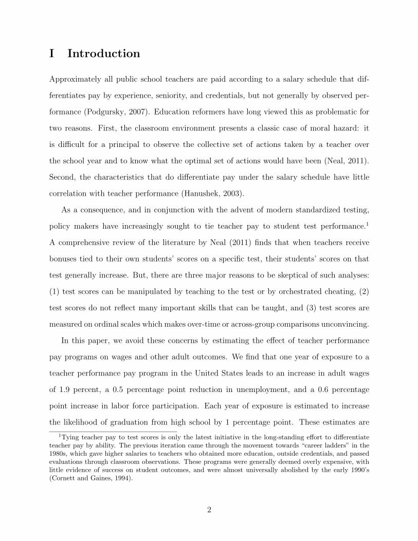
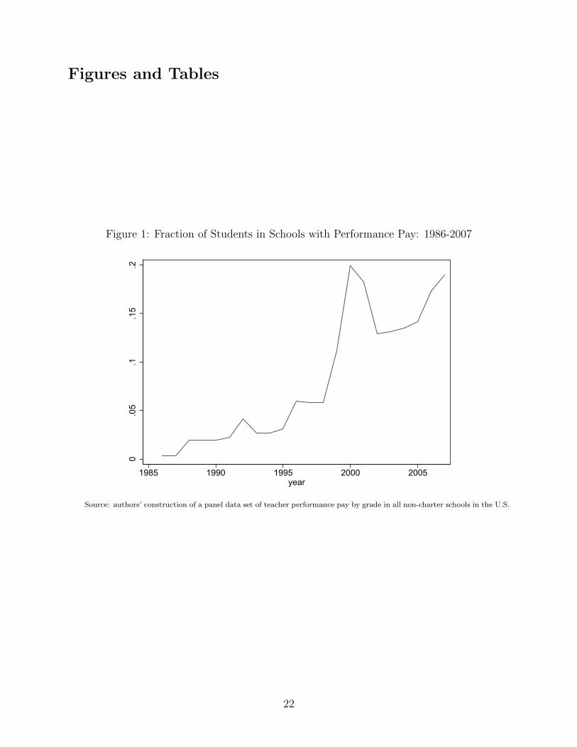
In Figure 1, we plot the fraction of non-charter public school children in the United States

who were enrolled in a school which offered performance pay from 1986-2007. Starting in the

early 1990s, teacher performance pay programs have been adopted by an increasing number

of schools. The figure shows that on average an additional 1 percentage point of students

were educated in schools with performance pay programs in each year since 1992. As of the

2007-2008 school year, 17 percent of students in the United States were being educated in

such a manner.

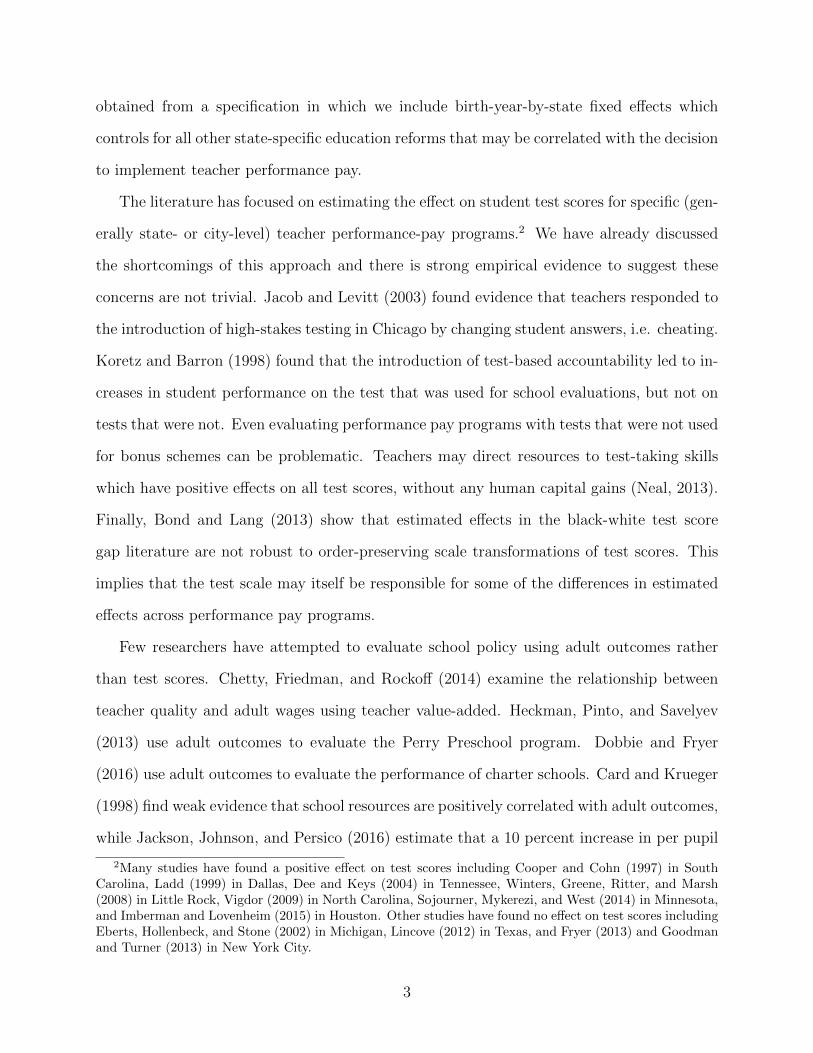
Figure 2 maps the fraction of non-charter public school children who were enrolled in a

school which offered performance pay by state in selected years. In the 1980s, only a small

number of school districts in Arizona offered test-based teacher performance pay. We see an

increase in performance pay in the 1990s in part due to the adoption of large-scale programs

in North Carolina, Florida, Georgia, and California, as well as several district-wide programs.

The trend continues into the 2000s with the growth of programs, for example, in Arizona

and Minnesota, and as a possible consequence of No Child Left Behind legislation making

tests more prevalent on which teacher performance pay can be based.9

Which Schools Offer Teacher Performance Pay?

In the 7 state-wide performance-pay programs in our study period, there is no differen-

tial selection as every public school in the state participated. However, in states where

performance-pay programs were instead implemented by school districts or individual schools,

the fraction of treated students ranges from 0.1 percent of students in Oklahoma in the late

9The low exposure we find early in our sample is supported by the literature. Porwoll (1979) finds thatonly 4% of districts in a national survey provided any sort of merit pay to teachers in 1978, though it isnot clear how frequently the merit pay was related to student test scores. In a qualitative study of 6 of theschools that Porwoll identified that still offered merit pay in 1983, Murnane and Cohen (1986) found thatnone related this pay to test scores, further supporting our low figures for this time period. A comprehensivesurvey by Cornett and Gaines (1994) suggests that test-based merit pay was virtually non-existent in thistime-period and our data reflects that. Ballou (2001) reports that 10% of public school teachers in 1993-1994were employed at a school which paid teachers merit pay, but again, it is not clear how frequently the meritpay is tied to student test scores. To our knowledge, our data set is the first that is able to track the completeset of merit pay programs that are explicitly linked to student test scores.

7

1980s and early 1990s to 46 percent of students in California in the early 2000s. Combining

these district- and school-level programs into groups by state and time period, we identi-

fied 28 separate state-periods where there were a large number of schools participating in

performance-pay programs. We group years together for a state if there is no break in the

program and if there is no large change in the number of participating schools.10

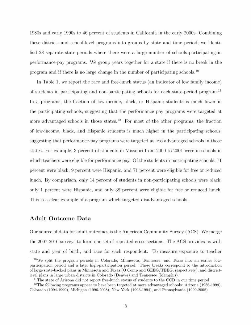
In Table 1, we report the race and free-lunch status (an indicator of low family income)

of students in participating and non-participating schools for each state-period program.11

In 5 programs, the fraction of low-income, black, or Hispanic students is much lower in

the participating schools, suggesting that the performance pay programs were targeted at

more advantaged schools in those states.12 For most of the other programs, the fraction

of low-income, black, and Hispanic students is much higher in the participating schools,

suggesting that performance-pay programs were targeted at less advantaged schools in those

states. For example, 3 percent of students in Missouri from 2000 to 2001 were in schools in

which teachers were eligible for performance pay. Of the students in participating schools, 71

percent were black, 9 percent were Hispanic, and 71 percent were eligible for free or reduced

lunch. By comparison, only 14 percent of students in non-participating schools were black,

only 1 percent were Hispanic, and only 38 percent were eligible for free or reduced lunch.

This is a clear example of a program which targeted disadvantaged schools.

Adult Outcome Data

Our source of data for adult outcomes is the American Community Survey (ACS). We merge

the 2007-2016 surveys to form one set of repeated cross-sections. The ACS provides us with

state and year of birth, and race for each respondent. To measure exposure to teacher

10We split the program periods in Colorado, Minnesota, Tennessee, and Texas into an earlier low-participation period and a later high-participation period. These breaks correspond to the introductionof large state-backed plans in Minnesota and Texas (Q Comp and GEEG/TEEG, respectively), and district-level plans in large urban districts in Colorado (Denver) and Tennessee (Memphis).

11The state of Arizona did not report free-lunch status of students to the CCD in our time period.12The following programs appear to have been targeted at more advantaged schools: Arizona (1986-1999),

Colorado (1994-1999), Michigan (1996-2008), New York (1993-1994), and Pennsylvania (1999-2008)

8

performance pay programs, we calculate the fraction of students in each grade in each state

and year by race who were enrolled in a school with performance pay. Assuming that a

student begins 1st grade at age six and 12th grade at age seventeen, we take the summation

of the fraction of students by race who were exposed over the 12 relevant years. Our measure

could thus be thought of as the expected number of years of education a student would have

had in schools where part of teacher pay was tied to student test scores conditional on their

race, and year and state of birth.13 For each individual, we also calculate exposure to a

teacher performance pay program by grade in order to differentiate the effects in grades 1-3,

4-6, 7-9, and 10-12.

We restrict attention to cohorts born after 1980, as earlier cohorts will have begun school-

ing before the CCD begins, and to individuals who were at least 23 years old at the time

of the survey. We further restrict our sample to full-time, year round workers, though we

include part-time and non-labor force participants in our robustness analysis.

While we know the birth state of each individual in our sample, we do not know whether

they were educated in the state in which they were born. Similar to Loeb and Page (2000),

we use two samples. Our main sample includes all individuals. These results will likely be

attenuated, as the uncertain location of education introduces measurement error into our

exposure variable.14 We will test the robustness of our results using a second sample which

only includes individuals who were living in their birth state the year prior to the ACS survey.

This sample will have a higher probability of having received the exposure we calculate for

them, but will produce negatively biased results if exposure to teacher performance pay

causes individuals to move to higher wage states.

As discussed in the section above, there is substantial variation across states and across

time in racial and socioeconomic characteristics of schools which adopt performance pay.

This implies that in many states, the likelihood of exposure to teacher performance pay

13Some students drop out of high school and never reach the 12th grade. We do not adjust the performancepay exposure measure for this as it is a possible outcome of the program.

14There could be an upward bias if the introduction of teacher performance pay causes families to moveto states with better education systems that do not have such programs.

9

differs significantly by race even for individuals in the same cohort. In calculating the

exposure measure, we use 4 race/ethnicity groups: white, black, Hispanic, and Asian. Table

2 reports the average years of exposure to teacher performance pay by race for both the full

sample and the sample of non-movers across all survey years and states by the grade-level

group of exposure. Performance pay exposure on average across these years is small. The

results shows that, conditional on being in a birth state-birth year cohort in which some

students had teachers eligible for performance pay, black students had roughly 0.5 more

years of exposure than white students, and 1 more year than Asian students. Table 2 also

indicates that the individuals in our sample were more likely to have a teacher eligible for

performance pay in high school than in middle or elementary school. This does not indicate

that elementary school teachers are less likely to be eligible for performance pay than high

school teachers, but is instead simply the result of our sample restrictions and, as shown in

Figure 1, the increasing number of schools offering performance pay from 1986 to 2007.

In Table 3, we report descriptive statistics for our ACS sample. Column (1) shows

estimates for the full sample and columns (2) and (3) break this sample down between

individuals who received zero and non-zero exposure, respectively. Conditional on being in

a state-cohort which had any performance pay, the average individual receives 1.30 years

of schooling at a school where teachers are eligible for performance pay. Cohorts with

high performance pay exposure have a higher fraction of minorities, particularly Hispanics,

reflecting the prevalence of these programs in the American Southwest. They appear to

have slightly lower wages and educational attainment, and are educated with slightly higher

student/teacher ratios. Average per pupil spending is similar across all columns.15 Columns

(4) through (6) repeat this analysis for the sample which excludes out-of-state movers, and

we observe similar patterns.

15Log mean school spending is the log of average per pupil spending as reported in the CCD and ismeasured only at the state-level. We interpolate missing nominal values and then convert them to realvalues using the CPI.

10

III Estimation Strategy

Our primary objective is to estimate the effect of an additional year of exposure to a teacher

incentive pay program on adult wages. We do this by first estimating

Yirtsy = α + β exposurersy + δt + λry + θrs + γXi + τWrsy + ωZsy + uirtsy. (1)

Y is our outcome variable (generally, log wage) for worker i of race/ethnicity r in year t

who was born in state s in year y. δt is a year fixed effect, λry is a race-specific birth year

fixed effect, θrs is a race-specific birth state fixed effect, and Xi, is a set of worker-specific

characteristics including gender and age squared.16 Wrsy is a set of race-, state-, and cohort-

specific school characteristics, which includes the student/teacher ratio, fraction of same-race

students in charter schools, fraction of classmates that are black, fraction of classmates that

are Hispanic, and fraction of classmates that are eligible for free and reduced lunch. Note

that each of these school characteristics are calculated separately by race in each state-year

and averaged over the years when individual i of race r is in grades 1 through 12. Zsy is a

set of state- and cohort-specific characteristics that may influence education quality but do

not vary within state, including log state-wide education spending per student averaged over

the years in grades 1 through 12 and years of Republican control of the state legislature and

governors office during grades 1 through 12.

We measure performance pay exposure as the expected number of years a student of

race r born in state s in year y would have been educated under a teacher who was eligible

for payments based on student test scores (see above). Given our controls, we identify β

from the timing of adoption and disparate exposure by race and ethnicity to teacher pay

for performance programs within a state. In other words, a positive estimate of β indicates

that generally black cohorts who had more teacher performance pay exposure earned higher

16The worker’s age is captured by the year and birth-year fixed effects. We include age squared to capturethe rapid returns to labor market experience in the mid-20’s. Note that we do not include a state of residencefixed effect as teacher performance pay may cause students to relocate.

11

wages as adults than black cohorts who had less teacher performance pay exposure in that

state, and similar for our other racial groups.

One lingering concern is that adopting a performance-pay program may be one of sev-

eral education reforms taken simultaneously. Our state- and cohort-specific Zsy controls

should partially account for this. However, an even stronger approach is to exploit within

cohort variation in exposure by including birth state-cohort fixed effects, φsy. Our preferred

specification is thus

Yirtsy = α + βexposurersy + δt + λry + θrs + φsy + γXi + τWrsy + uirtsy. (2)

Our identification comes off of variation in the racial gap by birth state-cohort in response

to within-cohort variation of teacher performance pay. In other words, a positive β would

indicate that cohorts in which black students were more frequently educated by teachers

who were eligible for performance pay relative to whites had a lower black-white wage gap

when they were adults, and similarly for other racial combinations. One downside of this

specification is that state-wide programs can no longer be used for identification; all of our

effects are estimated from only those programs listed in Table 1.

One important caveat for our results from equation 2 is that while φsy accounts for

any state-wide changes in education policy, we can only account for within-state variation in

school policy through our Wrsy controls. While we have measures of some important variables

at this level like student/teacher ratio, we do not have measures of per-pupil spending.

Moreover, performance pay programs that target, for example, black and hispanic children

may attract new, higher quality teachers from majority white districts, which would lead to

better minority and worse white outcomes simply through a change in teacher composition.

Thus our results should be interpreted cautiously as the effects of implementing a teacher

performance pay program at a small number of schools. General equilibrium effects may be

more muted.17

17However, as we discuss briefly in Section IV, state-wide programs appear to have been more successful

12

IV Results

We estimate equation 1, with log wage as the outcome, on the full sample of workers and

report the results in Table 4. With no additional controls, other than observation year fixed

effects and the birth year fixed effects, the point estimate implies that a one year increase in

effective exposure to a performance-pay program is associated with a 1.4 percent reduction

in wages. However, this reflects both that poorer performing school systems were more likely

to implement performance pay and that these programs were concentrated in the lower-wage

South. When we include birth state fixed effects in column (2), the negative bias is reduced

and the estimate becomes statistically indistinguishable from zero. Adding controls for race

as well as worker and school characteristics in column (3) pushes the estimate slightly above

zero.

Column (4) adds race-specific birth state and birth year fixed effects. The race-specific

birth fixed effects especially are important, as they account for, for example, states which

see large adoption of programs targeting black children because of large racial disparities in

that state. These controls raise our point estimate only slightly, but it becomes statistically

significant at the 10% level. The point estimate implies that a one year increase in exposure

to a performance-pay program would result in a 0.3 percent increase in early adult wages.

In columns (5) and (6) we estimate equation 2 by adding birth-year-by-birth-state fixed

effects.18 Column (5) excludes the set of school characteristic variables (student/teacher

ratio, fraction of same-race students in charter schools, fraction of classmates that are black,

fraction of classmates that are Hispanic, and fraction of classmates that are eligible for free

and reduced lunch), while column (6) includes these variables. When we identify the effects

only from within birth state-cohort variation in exposure, we find a substantially larger effect

of teacher performance pay. The estimate from column (6) implies that a one year increase

in exposure to a performance-pay program would result in statistically significant 1.9 percent

than small programs, which suggests general equilibrium effects may only be a small concern.18The school spending and Republican party control of state government measures only vary at the state-

cohort level, and so they are absorbed by these fixed effects.

13

increase in wages, and a 22 percent total gain for 12 full years of exposure. This is a slightly

larger effect than Chetty, Friedman, and Rockoff (2014) found for a one standard deviation

increase in teacher quality, and is roughly equivalent to a 33% increase in school spending

in each year based on estimates from Jackson, Johnson, and Persico (2016).

There are several explanations for the difference in our estimates form column (4) to

column (6). The most plausible reason to us is states/districts respond to declines in the

quality of their school system by implementing teacher performance pay. Thus, column (4)

is biased downwards because cohorts who received less performance pay had on average

higher quality schools during their education. This is backed up qualitatively in our data

itself, where we see many examples of programs that were implemented to try and improve

“failing” schools.19

However, it is important to note that, with birth state-cohort fixed effects, we identify

only off of states that have variation in exposure within race; i.e. we exclude state-wide

programs that cover every student. The difference between columns (4) and (6) could be

due to changes in the sample, however this does not appear to be case. In an unreported

robustness check, we re-estimated column (4) allowing the effect of exposure to vary by

whether or not the program covers all students in a state, and we find that state-wide

programs were more, not less, effective at raising adult wages than the smaller programs

which make up our identification.20

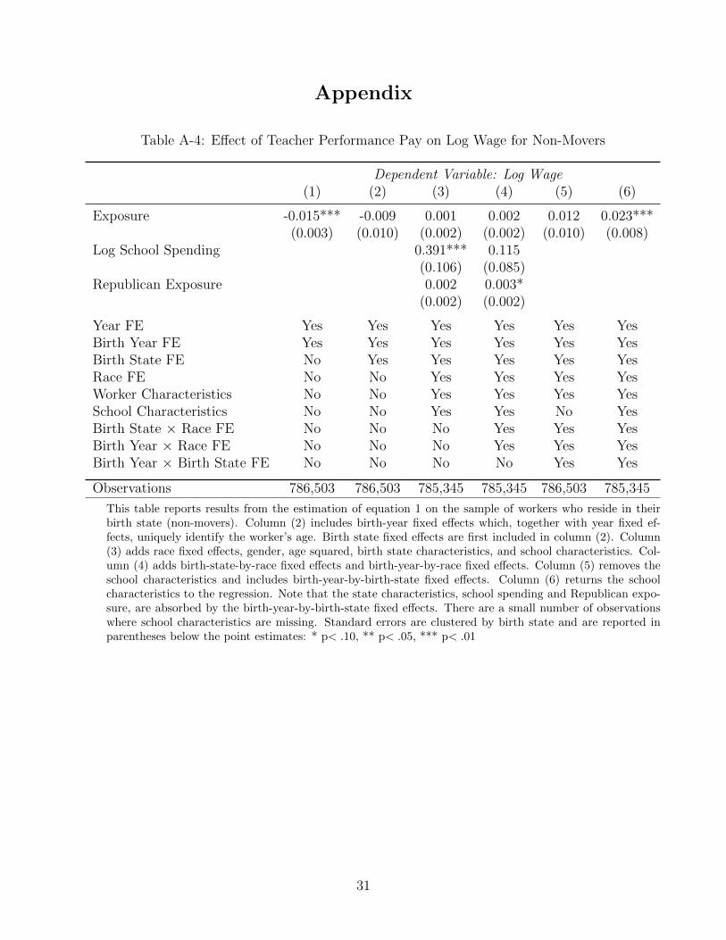
Results from the sample of individuals who reside in their birth state (non-movers) are

reported in the appendix and are very similar to those reported in Table 4. The column (6)

point estimate implies a 2.3 percent wage increase from a 1 year increase in exposure. This

similar but slightly larger estimate is consistent with our view that the full sample has a

greater level of measurement error which would cause attenuation bias.

19For example, the Effective Practice Incentive Community (EPIC) program in Memphis and the Districtof Columbia; the Teacher Recruitment and Student Support (TRSS) program in Los Angeles; and the MobileTransformation Plan in Mobile, Alabama.

20These results are available upon request.

14

Other Outcomes

Table 5 reports results from the estimation of equation 2 on other outcomes including unem-

ployment, labor force participation, full-time employment, years of education, and indicators

for high school and college graduation. We include the full set of controls, as in column (6) of

Table 4. The results generally suggest that performance pay programs have a positive effect

on both employment and education. A one year increase in exposure to a performance-pay

program causes a statistically significant 0.5 percentage point reduction in the probability of

unemployment, a statistically significant 0.6 percentage point increase in labor force partici-

pation, and a statistically insignificant 0.5 percentage point increase in full-time employment.

Note we exclude married women from the sample used in column (2) as their labor force par-

ticipation decision is different than for men and single women. The estimated small increase

in years of education seems to be driven by a statistically significant 1 percentage point

increase in the probability of graduating from high school, with only small and statistically

insignificant (but positive) estimates at other levels of education.

Heterogeneous Effects

In the first three columns of Table 6 we look for heterogeneous effects by interacting the

exposure variable with individual characteristics like race, gender, and educational attain-

ment. The results suggest no important heterogeneous effects by race, gender, or educational

attainment, with the exception of some evidence for a smaller, but still positive causal effect

for Hispanic students. Note that as Table 5 suggests that these programs had some positive

effects on education attainment itself, the effects by educational attainment may understate

any true heterogeneity, due to changes in the composition of the education groups.

Up to this point we have implicitly assumed that the effect of exposure is the same

regardless of the grade in which the child is exposed. There are many reasons to think this

is not the case. The child development literature, for instance, has found that interventions

earlier in life are more effective than those later in life (e.g., Cunha, Heckman, and Schennach,

15

2010). To test this assumption, in column (4) we split the exposure measure into four periods:

early grade school (grades 1-3), later grade school (grades 4-6), middle school (grades 7-9) and

high school (grades 10-12). Consistent with this literature we find that by far the strongest

effects come from exposure in grades 1 - 3. One year of exposure during these grades leads

to a 7.4 percent increase in adult wages, almost equivalent to the effect of moving from an

inexperienced to an experienced kindergarten teacher found by Chetty, Friedman, Hilger,

Saez, Schanzenbach, and Yagan (2011). We find mixed if any effects for exposure after third

grade.

Finally, in column (5) of Table 6 we look for heterogeneous effects by family income.

Using our program groups from Table 1, we classify a program as either “free-lunch focused”

or “not free-lunch focused” based on whether students exposed to performance pay in that

program had higher rates of free-lunch participancy than those not exposed to performance

pay.21 Recall that free-lunch participancy is a proxy for low-income students. The interaction

of an indicator for a free-lunch focused program with the exposure variable shows that the

positive effects are driven by those programs that were targeted at low-income schools. The

evidence suggests that programs that were concentrated on relatively high-income schools

had a negative (if any) effect on adult outcomes.

Placebo Tests

Finally, we perform a series of placebo tests in which we assign the performance pay exposure

variable for one group to a randomly chosen group which generates a placebo treatment.

This is repeated 100 times and the average values of the estimated effect and standard error

are reported in Table 7. Each replication uses the full sample of workers with the full set of

controls and fixed effects included, as in column (6) of Table 4. The dependent variable in all

columns is the log wage. Column (1) assigns the performance pay exposure measure for each

state to a randomly chosen state, keeping the racial targeting and timing in place. Column

21The programs with are not classified as free-lunch focused are Colorado, 1994-1999; Colorado, 1999-2008;Michigan, 1996-2008; New York, 1993-1994; and Pennsylvania, 1999-2008.

16

(2) assigns the performance pay exposure measure for each birth cohort to a randomly chosen

birth cohort in the actual birth state and for the actual race. Column (3) assigns the exposure

for each race and state to a randomly chosen race and state, maintaining the actual birth

year. Column (4) assigns the exposure for each birth year and state to a randomly chosen

birth year and state, maintaining the actual race. Column (5) assigns the exposure for each

birth year, birth state, and race to a randomly chosen birth year, state and race. In each

case, the results pass the placebo test.

V Discussion and Conclusion

In this paper we estimate the effect of teacher performance pay programs in the United

States on adult outcomes, primarily wages but also other labor market outcomes and educa-

tional attainment. This is in contrast to most of the literature which has evaluated teacher

performance pay through student test scores which can be manipulated and do not capture

important skills that are difficult to test but important in determining wages.

We construct a comprehensive data set of schools which have implemented teacher per-

formance pay programs across the United States since 1986. This enables us to calculate

the fraction of students by race in each grade in each state who attend a school in which the

teachers are eligible to receive additional pay based on student performance on a standardized

test. We believe our data is the most comprehensive such data set constructed.

We provide several strong words of caution. Our work does nothing to dispel concerns

about the misaligned incentives test-based performance pay packages can create. The the-

ory here is well-established, and a poorly designed program or poorly designed test could

certainly have negative effects on student learning. Likewise, our results in no way say that

student testing is the optimal way to incentivize teachers, or that the programs that have

been implemented are optimal. Our results merely suggest that teacher performance pay, as

it has been implemented in the United States, has generally led to better long-run outcomes

17

for those who are exposed to it than those who have not. It is without question that better

programs can be designed than those that currently exist, whether test-focused or not.

However, despite these caveats our results have important implications for the design of

teacher performance pay programs. First, our evidence suggests that the strongest positive

effects come from program exposure in the early grades. Research on child development has

been overwhelming in its emphasis on the importance of early interventions; teacher perfor-

mance pay appears to be no different. This presents an additional challenge to policymakers

as early childhood tests can be plagued with substantial measurement error (Bond and Lang,

2018).

Second, our results suggest that performance pay is not effective at improving outcomes

for those at already high achieving schools. We find a negative impact of programs that

disproportionately targeted schools with low free-lunch participation. Instead, the gains

come from programs at low-income (and likely under-performing schools). However, our

results indicate that black and Hispanic students are no more likely to benefit than white

and Asian students, who have higher socioeconomic status on average than their black and

Hispanic peers.

As such programs continue to expand in the United States, teacher performance pay

will remain an important area of future research. Our work is cautiously optimistic about

its long-run efficacy, but more work is needed to understand optimal program design, and

comparisons with innovative schooling practices.

18

References

Ballou, D., “Pay for Performance in Public and Private Schools,” Economics of Education Review,

20 (2001), 51–61.

Bond, T. N., and K. Lang, “The Evolution of the Black-White Test Score Gap in Grades K-3: The

Fragility of Results,” The Review of Economics and Statistics, 95 (2013), 1468–1479.

, “The Black-White Education Scaled Test-Score Gap in Grades K-7,” Journal of Human

Resources (2018).

Card, D., and A. B. Krueger, “School Resources and Student Outcomes,” The Annals of the

American Academy of Political and Social Science, 559 (1998), 39–53.

Chetty, R., J. N. Friedman, N. Hilger, E. Saez, D. W. Schanzenbach, and D. Yagan, “How does your

kindergarten classroom affect your earnings? Evidence from Project STAR,” Quarterly Journal

of Economics, 126 (2011).

Chetty, R., J. N. Friedman, and J. E. Rockoff, “Measuring the Impacts of Teachers II: Teacher

Value-Added and Student Outcomes in Adulthood,” The American Economic Review, 104

(2014), 2633–2679.

Cooper, S. T., and E. Cohn, “Estimation of a frontier production function for the South Carolina

educational process,” Economics of Education Review, 16 (1997), 313–327.

Cornett, L. M., and G. F. Gaines, “Reflecting on Ten Years of Incentive Programs: The 1993 SREB

Career Ladder Clearning House Survey,” Institute of Education Sciences ERIC No. ED378163

(1994).

Cunha, F., J. J. Heckman, and S. M. Schennach, “Estimating the Technology of Cognivie and

Noncognitive Skill Formation,” Econometrica, 78 (2010), 883–931.

Dee, T. S., and B. J. Keys, “Does merit pay reward good teachers? Evidence from a randomized

experiment,” Journal of Poli, 23 (2004), 471–488.

19

Dobbie, W., and R. G. Fryer, “Charter Schools and Labor Market Outcomes,” Working Paper

(2016).

Eberts, R., K. Hollenbeck, and J. Stone, “Teacher Performance Incentives and Student Outcomes,”

Journal of Human Resources, 37 (2002), 913–927.

Fryer, R. G., “Teacher Incentives and Student Achievement: Evidence from New York City Public

Schools,” Journal of Labor Economics, 31 (2013), 373–407.

Goodman, S. F., and L. J. Turner, “The Design of Teacher Incentive Pay and Educational Out-

comes: Evidence from the New York City Bonus Program,” Journal of Labor Economics (2013).

Hanushek, E. A., “The Failure of Input-Based Resource Policies,” Economic Journal, 113 (2003),

F64–F98.

Heckman, J., R. Pinto, and P. Savelyev, “UnderOutcomes the Mechanisms Through Which an In-

fluential Early Childhood Program Boosted Adult Outcomes,” The American Economic Review,

103 (2013), 1–35.

Imberman, S. A., and M. F. Lovenheim, “Incentive Strength and Teacher Productivity: Evidence

From a Group-Based Teacher Incentive Pay System,” The Review of Economics and Statistics,

97 (2015), 364–386.

Jackson, C. K., R. C. Johnson, and C. Persico, “The Effects of School Spending on Educational

and Economic Outcomes: Evidence from School Finance Reforms,” The Quarterly Journal of

Economics, 131 (2016), 157–218.

Jacob, B. A., and S. D. Levitt, “Rotten Apples: An Investigation of the Prevalance of Predictors

of Teacher Cheating,” Quarterly Journal of Economics, 118 (2003), 843–877.

Koretz, D., and S. Barron, (1998) The Validity of Gains in Scores on the Kentucky Instructional

Results Information System (KIRIS). RAND.

Ladd, H. F., “The Dallas School Accountability and Incentive Program: an Evaluation of its Impact

on Student Outcomes,” Economics of Education Review, 18 (1999), 1–16.

20

Lavy, V., “Teachers’ Pay for Performance in the Long-Run: Effects on Students’ Educational and

Labor Market Outcomes in Adulthood,” NBER Working Paper No. 20983 (2015).

Lincove, J. A., “Can Teacher Incentive Pay Improve Student Performance on Standardized Tests?,”

Working Paper (2012).

Loeb, S., and M. E. Page, “Examining the Link between Teacher Wages and Student Outcomes:

The Importance of Alternative Labor Market Opportunities and Non-Pecuniary Variation,” Re-

view of Economics and Statistics, 82 (2000), 393–408.

Murnane, R. J., and D. K. Cohen, “Merit Pay and the Evaluation Problem,” Harvard Educational

Review (1986).

Neal, D., (2011) Handbook of the Economics of Educationchap. The Design of Performance Pay in

Education, 495–550. Elsevier.

, “The Consequences of Using One Assessment System to Pursue Two Objectives,” Journal

of Economic Education (2013).

Podgursky, M., “Teams versus Bureaucracies: Personnel Policy, Wage-Setting, and Teacher Quality

in Traditional Public, Charter, and Private Schools,” in Charter School Outcomes. Mahwah, NJ:

Lawrence Erlbaum Associates, Inc. (2007).

Porwoll, P. J., (1979) Merit Pay for Teachers. Arlington, Va. Educational Research Service.

Sojourner, A. J., E. Mykerezi, and K. L. West, “Teacher Pay Reform and Productivity: Panel

Data Evidence from Adoptions of Q-Comp in Minnesota,” The Journal of Human Resources, 49

(2014), 945–981.

Vigdor, J. L., (2009) Performance Incentives: Their Growing Impact on American K-12 Educa-

tionchap. Teacher Salary Bonuses in North Carolina. Brookings.

Winters, M., J. P. Greene, G. Ritter, and R. Marsh, “The Effect of Performace-Pay in Little Rock,

Arkansas on Student Achievement,” National Center on Performace Incentives at Vanderbilt

University Working Paper 2008-02 (2008).

21

Figures and Tables

Figure 1: Fraction of Students in Schools with Performance Pay: 1986-2007

0.0

5.1

.15

.2

1985 1990 1995 2000 2005year

Source: authors’ construction of a panel data set of teacher performance pay by grade in all non-charter schools in the U.S.

22

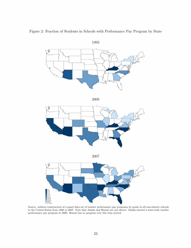
Figure 2: Fraction of Students in Schools with Performance Pay Program by State

1993

2000

2007

(.9,1](.5,.9](.4,.5](.3,.4](.2,.3](.15,.2](.1,.15](.06,.1](.03,.06](.02,.03](.01,.02](.005,.01][0,.005]No Program

Source: authors construction of a panel data set of teacher performance pay programs by grade in all non-charter schoolsin the United States from 1986 to 2007. Note that Alaska and Hawaii are not shown. Alaska started a state-wide teacherperformance pay program in 2006. Hawaii has no program over this time period.

23

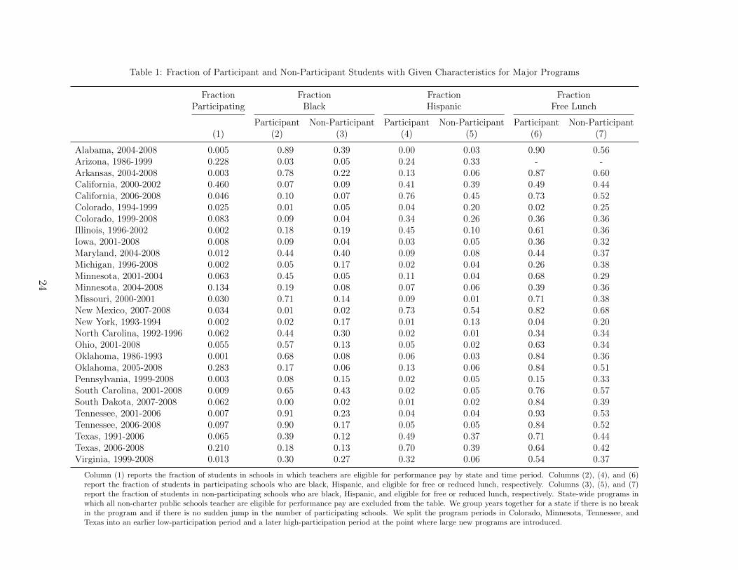
Table 1: Fraction of Participant and Non-Participant Students with Given Characteristics for Major Programs

Fraction Fraction Fraction FractionParticipating Black Hispanic Free Lunch

Participant Non-Participant Participant Non-Participant Participant Non-Participant(1) (2) (3) (4) (5) (6) (7)

Alabama, 2004-2008 0.005 0.89 0.39 0.00 0.03 0.90 0.56Arizona, 1986-1999 0.228 0.03 0.05 0.24 0.33 - -Arkansas, 2004-2008 0.003 0.78 0.22 0.13 0.06 0.87 0.60California, 2000-2002 0.460 0.07 0.09 0.41 0.39 0.49 0.44California, 2006-2008 0.046 0.10 0.07 0.76 0.45 0.73 0.52Colorado, 1994-1999 0.025 0.01 0.05 0.04 0.20 0.02 0.25Colorado, 1999-2008 0.083 0.09 0.04 0.34 0.26 0.36 0.36Illinois, 1996-2002 0.002 0.18 0.19 0.45 0.10 0.61 0.36Iowa, 2001-2008 0.008 0.09 0.04 0.03 0.05 0.36 0.32Maryland, 2004-2008 0.012 0.44 0.40 0.09 0.08 0.44 0.37Michigan, 1996-2008 0.002 0.05 0.17 0.02 0.04 0.26 0.38Minnesota, 2001-2004 0.063 0.45 0.05 0.11 0.04 0.68 0.29Minnesota, 2004-2008 0.134 0.19 0.08 0.07 0.06 0.39 0.36Missouri, 2000-2001 0.030 0.71 0.14 0.09 0.01 0.71 0.38New Mexico, 2007-2008 0.034 0.01 0.02 0.73 0.54 0.82 0.68New York, 1993-1994 0.002 0.02 0.17 0.01 0.13 0.04 0.20North Carolina, 1992-1996 0.062 0.44 0.30 0.02 0.01 0.34 0.34Ohio, 2001-2008 0.055 0.57 0.13 0.05 0.02 0.63 0.34Oklahoma, 1986-1993 0.001 0.68 0.08 0.06 0.03 0.84 0.36Oklahoma, 2005-2008 0.283 0.17 0.06 0.13 0.06 0.84 0.51Pennsylvania, 1999-2008 0.003 0.08 0.15 0.02 0.05 0.15 0.33South Carolina, 2001-2008 0.009 0.65 0.43 0.02 0.05 0.76 0.57South Dakota, 2007-2008 0.062 0.00 0.02 0.01 0.02 0.84 0.39Tennessee, 2001-2006 0.007 0.91 0.23 0.04 0.04 0.93 0.53Tennessee, 2006-2008 0.097 0.90 0.17 0.05 0.05 0.84 0.52Texas, 1991-2006 0.065 0.39 0.12 0.49 0.37 0.71 0.44Texas, 2006-2008 0.210 0.18 0.13 0.70 0.39 0.64 0.42Virginia, 1999-2008 0.013 0.30 0.27 0.32 0.06 0.54 0.37

Column (1) reports the fraction of students in schools in which teachers are eligible for performance pay by state and time period. Columns (2), (4), and (6)report the fraction of students in participating schools who are black, Hispanic, and eligible for free or reduced lunch, respectively. Columns (3), (5), and (7)report the fraction of students in non-participating schools who are black, Hispanic, and eligible for free or reduced lunch, respectively. State-wide programs inwhich all non-charter public schools teacher are eligible for performance pay are excluded from the table. We group years together for a state if there is no breakin the program and if there is no sudden jump in the number of participating schools. We split the program periods in Colorado, Minnesota, Tennessee, andTexas into an earlier low-participation period and a later high-participation period at the point where large new programs are introduced.

24

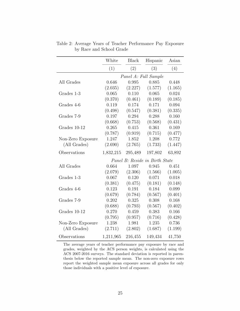
Table 2: Average Years of Teacher Performance Pay Exposureby Race and School Grade

White Black Hispanic Asian

(1) (2) (3) (4)

Panel A: Full SampleAll Grades 0.646 0.995 0.885 0.448

(2.035) (2.227) (1.577) (1.165)Grades 1-3 0.065 0.110 0.065 0.024

(0.370) (0.461) (0.189) (0.185)Grades 4-6 0.119 0.174 0.171 0.094

(0.498) (0.547) (0.381) (0.335)Grades 7-9 0.197 0.294 0.288 0.160

(0.668) (0.753) (0.568) (0.431)Grades 10-12 0.265 0.415 0.361 0.169

(0.787) (0.919) (0.715) (0.477)Non-Zero Exposure 1.247 1.852 1.208 0.772

(All Grades) (2.690) (2.765) (1.733) (1.447)

Observations 1,832,215 295,489 197,802 63,892

Panel B: Reside in Birth StateAll Grades 0.664 1.097 0.945 0.451

(2.079) (2.306) (1.566) (1.005)Grades 1-3 0.067 0.120 0.071 0.018

(0.381) (0.475) (0.181) (0.148)Grades 4-6 0.123 0.191 0.184 0.099

(0.679) (0.784) (0.567) (0.401)Grades 7-9 0.202 0.325 0.308 0.168

(0.688) (0.793) (0.567) (0.402)Grades 10-12 0.270 0.459 0.383 0.166

(0.795) (0.957) (0.716) (0.428)Non-Zero Exposure 1.238 1.981 1.235 0.736

(All Grades) (2.711) (2.802) (1.687) (1.199)

Observations 1,211,965 216,455 149,434 41,750

The average years of teacher performance pay exposure by race andgrades, weighted by the ACS person weights, is calculated using theACS 2007-2016 surveys. The standard deviation is reported in paren-thesis below the reported sample mean. The non-zero exposure rowsreport the weighted sample mean exposure across all grades for onlythose individuals with a positive level of exposure.

25

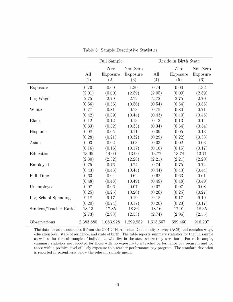
Table 3: Sample Descriptive Statistics

Full Sample Reside in Birth State

Zero Non-Zero Zero Non-ZeroAll Exposure Exposure All Exposure Exposure(1) (2) (3) (4) (5) (6)

Exposure 0.70 0.00 1.30 0.74 0.00 1.32(2.01) (0.00) (2.59) (2.05) (0.00) (2.59)

Log Wage 2.75 2.79 2.72 2.72 2.75 2.70(0.56) (0.56) (0.56) (0.54) (0.54) (0.55)

White 0.77 0.81 0.73 0.75 0.80 0.71(0.42) (0.39) (0.44) (0.43) (0.40) (0.45)

Black 0.12 0.12 0.13 0.13 0.13 0.14(0.33) (0.32) (0.33) (0.34) (0.34) (0.34)

Hispanic 0.08 0.05 0.11 0.09 0.05 0.13(0.28) (0.21) (0.32) (0.29) (0.22) (0.33)

Asian 0.03 0.02 0.03 0.03 0.02 0.03(0.16) (0.16) (0.17) (0.16) (0.15) (0.17)

Education 13.95 14.00 13.90 13.72 13.74 13.71(2.30) (2.32) (2.28) (2.21) (2.21) (2.20)

Employed 0.75 0.76 0.74 0.74 0.75 0.74(0.43) (0.43) (0.44) (0.44) (0.43) (0.44)

Full-Time 0.63 0.64 0.62 0.62 0.63 0.61(0.48) (0.48) (0.49) (0.49) (0.48) (0.49)

Unemployed 0.07 0.06 0.07 0.07 0.07 0.08(0.25) (0.25) (0.26) (0.26) (0.25) (0.27)

Log School Spending 9.18 9.17 9.19 9.18 9.17 9.19(0.20) (0.24) (0.17) (0.20) (0.23) (0.17)

Student/Teacher Ratio 18.13 17.85 18.36 18.16 17.91 18.35(2.73) (2.93) (2.53) (2.74) (2.96) (2.55)

Observations 2,383,880 1,083,928 1,299,952 1,615,667 699,460 916,207

The data for adult outcomes if from the 2007-2016 American Community Survey (ACS) and contains wage,education level, state of residence, and state of birth. The table reports summary statistics for the full sampleas well as for the sub-sample of individuals who live in the state where they were born. For each sample,summary statistics are reported for those with no exposure to a teacher performance pay program and forthose with a positive level of likely exposure to a teacher performance pay program. The standard deviationis reported in parenthesis below the relevant sample mean.

26

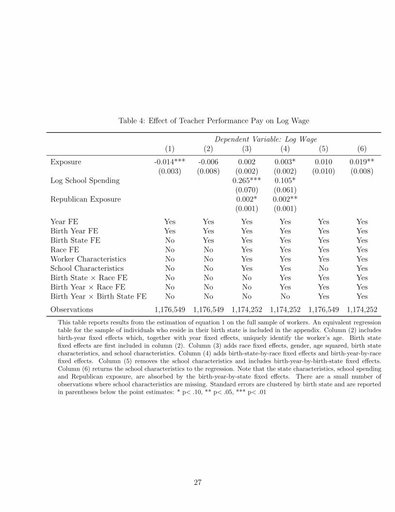
Table 4: Effect of Teacher Performance Pay on Log Wage

Dependent Variable: Log Wage(1) (2) (3) (4) (5) (6)

Exposure -0.014*** -0.006 0.002 0.003* 0.010 0.019**(0.003) (0.008) (0.002) (0.002) (0.010) (0.008)

Log School Spending 0.265*** 0.105*(0.070) (0.061)

Republican Exposure 0.002* 0.002**(0.001) (0.001)

Year FE Yes Yes Yes Yes Yes YesBirth Year FE Yes Yes Yes Yes Yes YesBirth State FE No Yes Yes Yes Yes YesRace FE No No Yes Yes Yes YesWorker Characteristics No No Yes Yes Yes YesSchool Characteristics No No Yes Yes No YesBirth State × Race FE No No No Yes Yes YesBirth Year × Race FE No No No Yes Yes YesBirth Year × Birth State FE No No No No Yes Yes

Observations 1,176,549 1,176,549 1,174,252 1,174,252 1,176,549 1,174,252

This table reports results from the estimation of equation 1 on the full sample of workers. An equivalent regressiontable for the sample of individuals who reside in their birth state is included in the appendix. Column (2) includesbirth-year fixed effects which, together with year fixed effects, uniquely identify the worker’s age. Birth statefixed effects are first included in column (2). Column (3) adds race fixed effects, gender, age squared, birth statecharacteristics, and school characteristics. Column (4) adds birth-state-by-race fixed effects and birth-year-by-racefixed effects. Column (5) removes the school characteristics and includes birth-year-by-birth-state fixed effects.Column (6) returns the school characteristics to the regression. Note that the state characteristics, school spendingand Republican exposure, are absorbed by the birth-year-by-state fixed effects. There are a small number ofobservations where school characteristics are missing. Standard errors are clustered by birth state and are reportedin parentheses below the point estimates: * p< .10, ** p< .05, *** p< .01

27

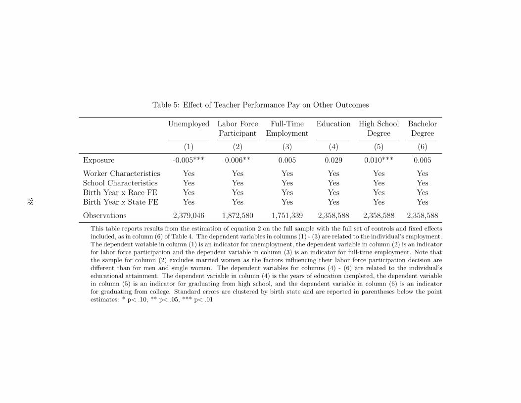
Table 5: Effect of Teacher Performance Pay on Other Outcomes

Unemployed Labor Force Full-Time Education High School BachelorParticipant Employment Degree Degree

(1) (2) (3) (4) (5) (6)

Exposure -0.005*** 0.006** 0.005 0.029 0.010*** 0.005

Worker Characteristics Yes Yes Yes Yes Yes YesSchool Characteristics Yes Yes Yes Yes Yes YesBirth Year x Race FE Yes Yes Yes Yes Yes YesBirth Year x State FE Yes Yes Yes Yes Yes Yes

Observations 2,379,046 1,872,580 1,751,339 2,358,588 2,358,588 2,358,588

This table reports results from the estimation of equation 2 on the full sample with the full set of controls and fixed effectsincluded, as in column (6) of Table 4. The dependent variables in columns (1) - (3) are related to the individual’s employment.The dependent variable in column (1) is an indicator for unemployment, the dependent variable in column (2) is an indicatorfor labor force participation and the dependent variable in column (3) is an indicator for full-time employment. Note thatthe sample for column (2) excludes married women as the factors influencing their labor force participation decision aredifferent than for men and single women. The dependent variables for columns (4) - (6) are related to the individual’seducational attainment. The dependent variable in column (4) is the years of education completed, the dependent variablein column (5) is an indicator for graduating from high school, and the dependent variable in column (6) is an indicatorfor graduating from college. Standard errors are clustered by birth state and are reported in parentheses below the pointestimates: * p< .10, ** p< .05, *** p< .01

28

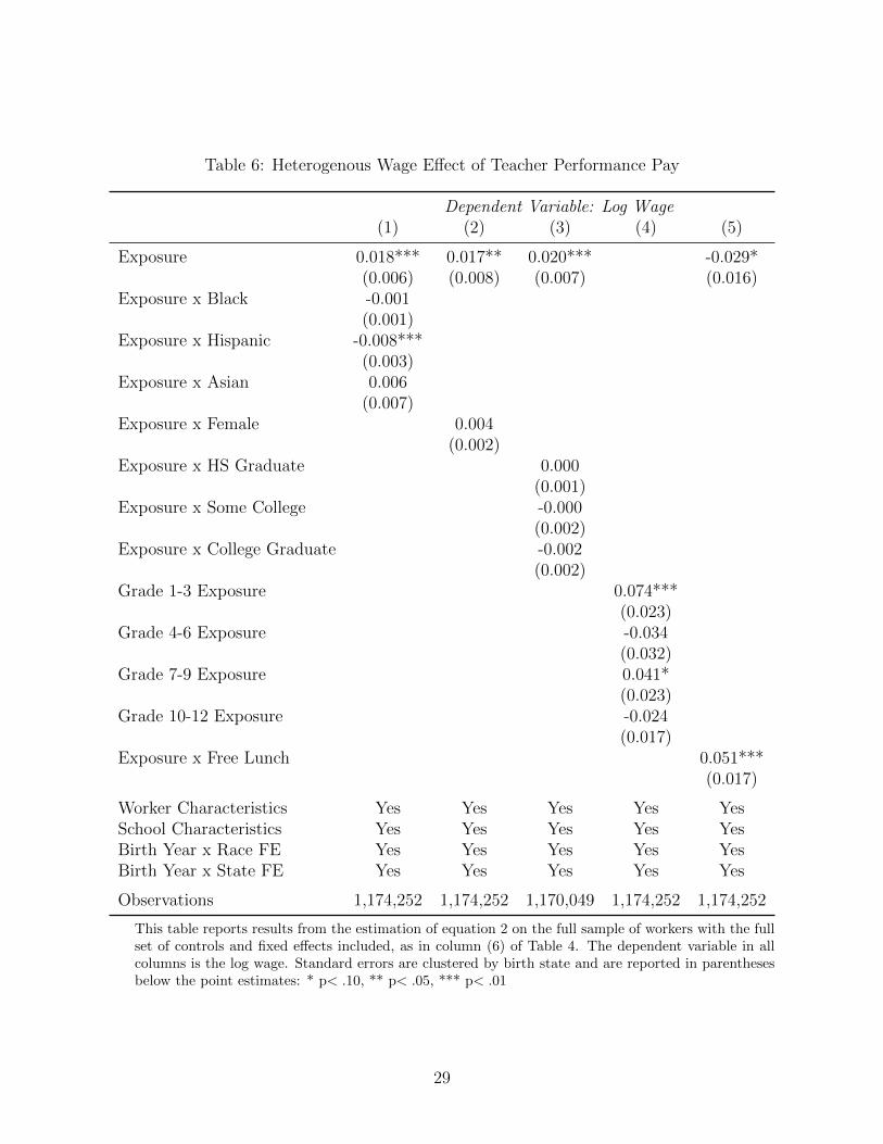
Table 6: Heterogenous Wage Effect of Teacher Performance Pay

Dependent Variable: Log Wage(1) (2) (3) (4) (5)

Exposure 0.018*** 0.017** 0.020*** -0.029*(0.006) (0.008) (0.007) (0.016)

Exposure x Black -0.001(0.001)

Exposure x Hispanic -0.008***(0.003)

Exposure x Asian 0.006(0.007)

Exposure x Female 0.004(0.002)

Exposure x HS Graduate 0.000(0.001)

Exposure x Some College -0.000(0.002)

Exposure x College Graduate -0.002(0.002)

Grade 1-3 Exposure 0.074***(0.023)

Grade 4-6 Exposure -0.034(0.032)

Grade 7-9 Exposure 0.041*(0.023)

Grade 10-12 Exposure -0.024(0.017)

Exposure x Free Lunch 0.051***(0.017)

Worker Characteristics Yes Yes Yes Yes YesSchool Characteristics Yes Yes Yes Yes YesBirth Year x Race FE Yes Yes Yes Yes YesBirth Year x State FE Yes Yes Yes Yes Yes

Observations 1,174,252 1,174,252 1,170,049 1,174,252 1,174,252

This table reports results from the estimation of equation 2 on the full sample of workers with the fullset of controls and fixed effects included, as in column (6) of Table 4. The dependent variable in allcolumns is the log wage. Standard errors are clustered by birth state and are reported in parenthesesbelow the point estimates: * p< .10, ** p< .05, *** p< .01

29

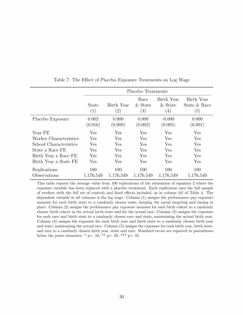
Table 7: The Effect of Placebo Exposure Treatments on Log Wage

Placebo Treatments

Race Birth Year Birth YearState Birth Year & State & State State & Race(1) (2) (3) (4) (5)

Placebo Exposure 0.002 0.000 0.000 -0.000 0.000(0.016) (0.009) (0.002) (0.005) (0.001)

Year FE Yes Yes Yes Yes YesWorker Characteristics Yes Yes Yes Yes YesSchool Characteristics Yes Yes Yes Yes YesState x Race FE Yes Yes Yes Yes YesBirth Year x Race FE Yes Yes Yes Yes YesBirth Year x State FE Yes Yes Yes Yes Yes

Replications 100 100 100 100 100Observations 1,176,549 1,176,549 1,176,549 1,176,549 1,176,549

This table reports the average value from 100 replications of the estimation of equation 2 where theexposure variable has been replaced with a placebo treatment. Each replication uses the full sampleof workers with the full set of controls and fixed effects included, as in column (6) of Table 4. Thedependent variable in all columns is the log wage. Column (1) assigns the performance pay exposuremeasure for each birth state to a randomly chosen state, keeping the racial targeting and timing inplace. Column (2) assigns the performance pay exposure measure for each birth cohort to a randomlychosen birth cohort in the actual birth state and for the actual race. Column (3) assigns the exposurefor each race and birth state to a randomly chosen race and state, maintaining the actual birth year.Column (4) assigns the exposure for each birth year and birth state to a randomly chosen birth yearand state, maintaining the actual race. Column (5) assigns the exposure for each birth year, birth state,and race to a randomly chosen birth year, state and race. Standard errors are reported in parenthesesbelow the point estimates: * p< .10, ** p< .05, *** p< .01

30

Appendix

Table A-4: Effect of Teacher Performance Pay on Log Wage for Non-Movers

Dependent Variable: Log Wage(1) (2) (3) (4) (5) (6)

Exposure -0.015*** -0.009 0.001 0.002 0.012 0.023***(0.003) (0.010) (0.002) (0.002) (0.010) (0.008)

Log School Spending 0.391*** 0.115(0.106) (0.085)

Republican Exposure 0.002 0.003*(0.002) (0.002)

Year FE Yes Yes Yes Yes Yes YesBirth Year FE Yes Yes Yes Yes Yes YesBirth State FE No Yes Yes Yes Yes YesRace FE No No Yes Yes Yes YesWorker Characteristics No No Yes Yes Yes YesSchool Characteristics No No Yes Yes No YesBirth State × Race FE No No No Yes Yes YesBirth Year × Race FE No No No Yes Yes YesBirth Year × Birth State FE No No No No Yes Yes

Observations 786,503 786,503 785,345 785,345 786,503 785,345

This table reports results from the estimation of equation 1 on the sample of workers who reside in theirbirth state (non-movers). Column (2) includes birth-year fixed effects which, together with year fixed ef-fects, uniquely identify the worker’s age. Birth state fixed effects are first included in column (2). Column(3) adds race fixed effects, gender, age squared, birth state characteristics, and school characteristics. Col-umn (4) adds birth-state-by-race fixed effects and birth-year-by-race fixed effects. Column (5) removes theschool characteristics and includes birth-year-by-birth-state fixed effects. Column (6) returns the schoolcharacteristics to the regression. Note that the state characteristics, school spending and Republican expo-sure, are absorbed by the birth-year-by-birth-state fixed effects. There are a small number of observationswhere school characteristics are missing. Standard errors are clustered by birth state and are reported inparentheses below the point estimates: * p< .10, ** p< .05, *** p< .01

31

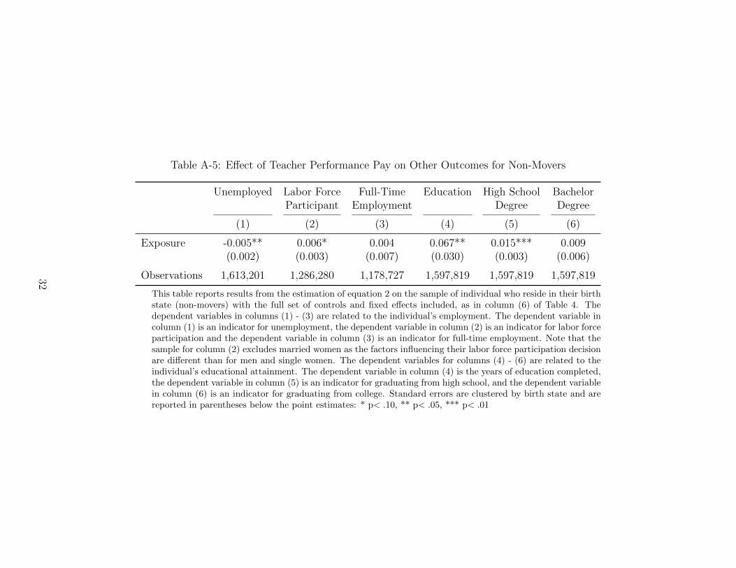
Table A-5: Effect of Teacher Performance Pay on Other Outcomes for Non-Movers

Unemployed Labor Force Full-Time Education High School BachelorParticipant Employment Degree Degree

(1) (2) (3) (4) (5) (6)

Exposure -0.005** 0.006* 0.004 0.067** 0.015*** 0.009(0.002) (0.003) (0.007) (0.030) (0.003) (0.006)

Observations 1,613,201 1,286,280 1,178,727 1,597,819 1,597,819 1,597,819

This table reports results from the estimation of equation 2 on the sample of individual who reside in their birthstate (non-movers) with the full set of controls and fixed effects included, as in column (6) of Table 4. Thedependent variables in columns (1) - (3) are related to the individual’s employment. The dependent variable incolumn (1) is an indicator for unemployment, the dependent variable in column (2) is an indicator for labor forceparticipation and the dependent variable in column (3) is an indicator for full-time employment. Note that thesample for column (2) excludes married women as the factors influencing their labor force participation decisionare different than for men and single women. The dependent variables for columns (4) - (6) are related to theindividual’s educational attainment. The dependent variable in column (4) is the years of education completed,the dependent variable in column (5) is an indicator for graduating from high school, and the dependent variablein column (6) is an indicator for graduating from college. Standard errors are clustered by birth state and arereported in parentheses below the point estimates: * p< .10, ** p< .05, *** p< .01

32

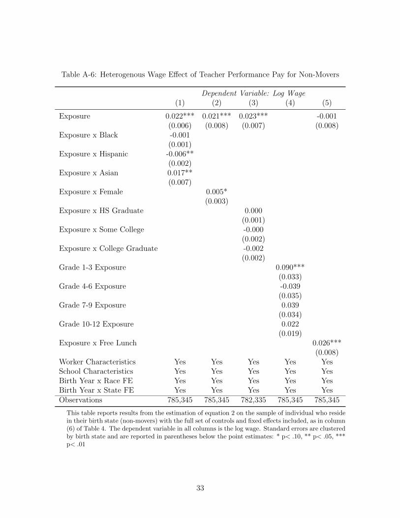
Table A-6: Heterogenous Wage Effect of Teacher Performance Pay for Non-Movers

Dependent Variable: Log Wage(1) (2) (3) (4) (5)

Exposure 0.022*** 0.021*** 0.023*** -0.001(0.006) (0.008) (0.007) (0.008)

Exposure x Black -0.001(0.001)

Exposure x Hispanic -0.006**(0.002)

Exposure x Asian 0.017**(0.007)

Exposure x Female 0.005*(0.003)

Exposure x HS Graduate 0.000(0.001)

Exposure x Some College -0.000(0.002)

Exposure x College Graduate -0.002(0.002)

Grade 1-3 Exposure 0.090***(0.033)

Grade 4-6 Exposure -0.039(0.035)

Grade 7-9 Exposure 0.039(0.034)

Grade 10-12 Exposure 0.022(0.019)

Exposure x Free Lunch 0.026***(0.008)

Worker Characteristics Yes Yes Yes Yes YesSchool Characteristics Yes Yes Yes Yes YesBirth Year x Race FE Yes Yes Yes Yes YesBirth Year x State FE Yes Yes Yes Yes YesObservations 785,345 785,345 782,335 785,345 785,345

This table reports results from the estimation of equation 2 on the sample of individual who residein their birth state (non-movers) with the full set of controls and fixed effects included, as in column(6) of Table 4. The dependent variable in all columns is the log wage. Standard errors are clusteredby birth state and are reported in parentheses below the point estimates: * p< .10, ** p< .05, ***p< .01

33