Taxonomy of Small Bodies

AS3141 Benda Kecil dalam Tata SuryaProdi Astronomi 2007/2008

B. Dermawan

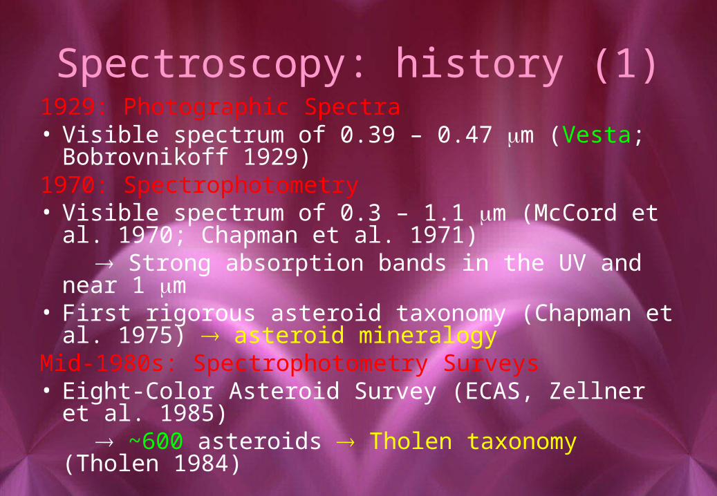
Spectroscopy: history (1)1929: Photographic Spectra• Visible spectrum of 0.39 – 0.47 m (Vesta;

Bobrovnikoff 1929)1970: Spectrophotometry• Visible spectrum of 0.3 – 1.1 m (McCord et al. 1970;

Chapman et al. 1971) Strong absorption bands in the UV and near 1 m• First rigorous asteroid taxonomy (Chapman et al.

1975) asteroid mineralogyMid-1980s: Spectrophotometry Surveys• Eight-Color Asteroid Survey (ECAS, Zellner et al.

1985) ~600 asteroids Tholen taxonomy (Tholen 1984)

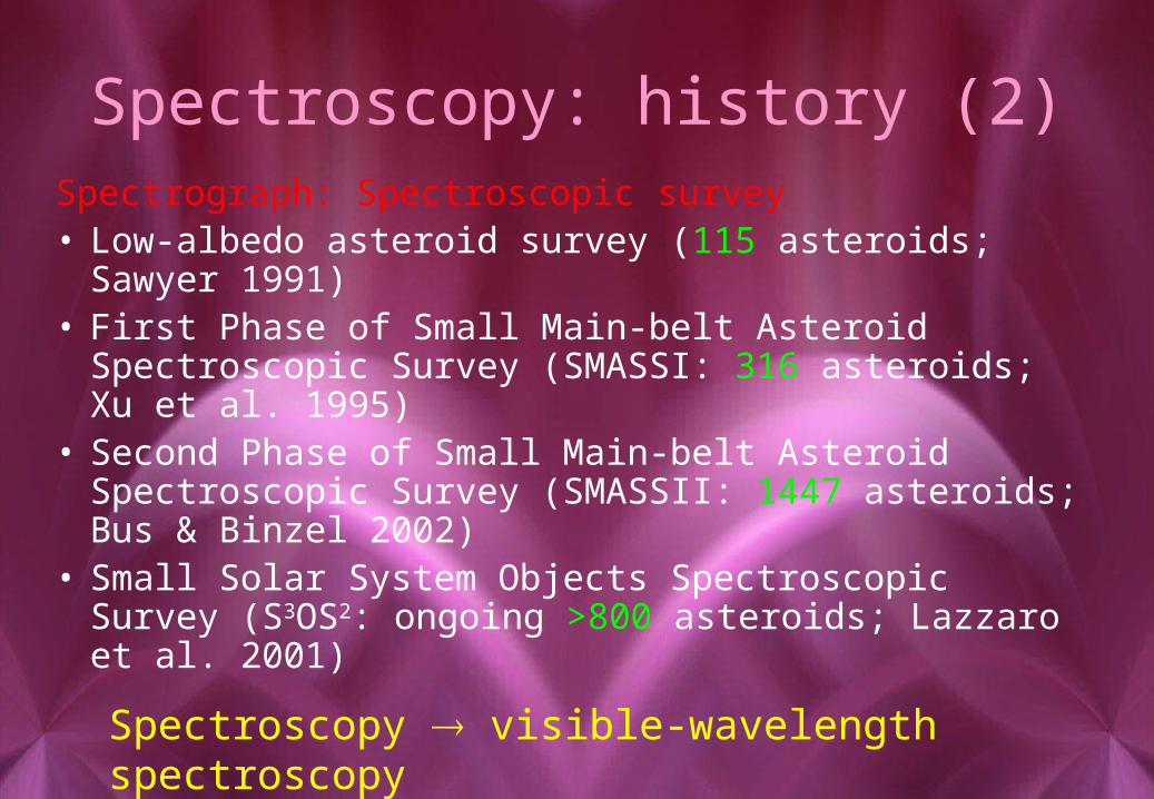
Spectroscopy: history (2)Spectrograph: Spectroscopic survey• Low-albedo asteroid survey (115 asteroids; Sawyer

1991)• First Phase of Small Main-belt Asteroid Spectroscopic

Survey (SMASSI: 316 asteroids; Xu et al. 1995)• Second Phase of Small Main-belt Asteroid

Spectroscopic Survey (SMASSII: 1447 asteroids; Bus & Binzel 2002)

• Small Solar System Objects Spectroscopic Survey (S3OS2: ongoing >800 asteroids; Lazzaro et al. 2001)

Spectroscopy visible-wavelength spectroscopy

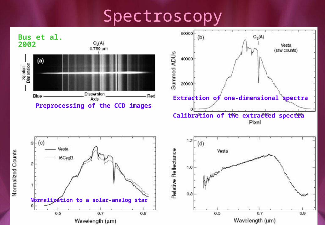
SpectroscopyBus et al. 2002

Preprocessing of the CCD imagesExtraction of one-dimensional spectra

Calibration of the extracted spectra

Normalization to a solar-analog star

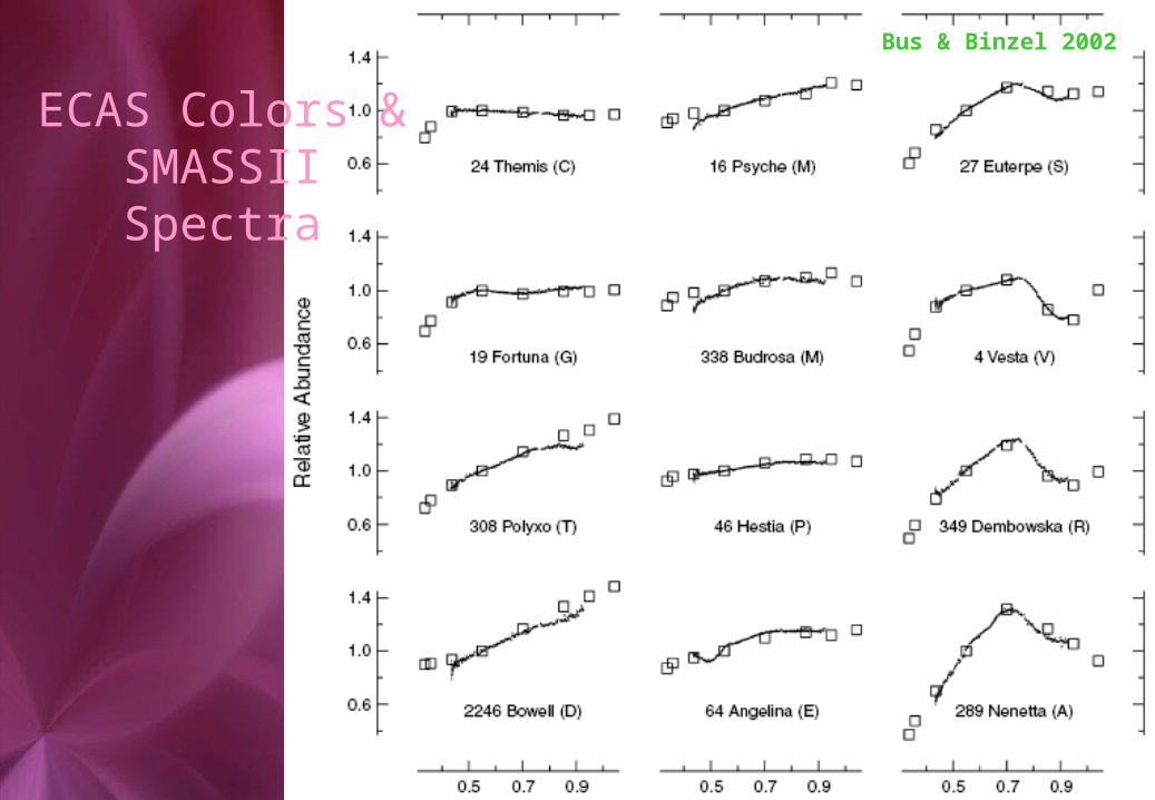
Bus & Binzel 2002

ECAS Colors & SMASSII Spectra

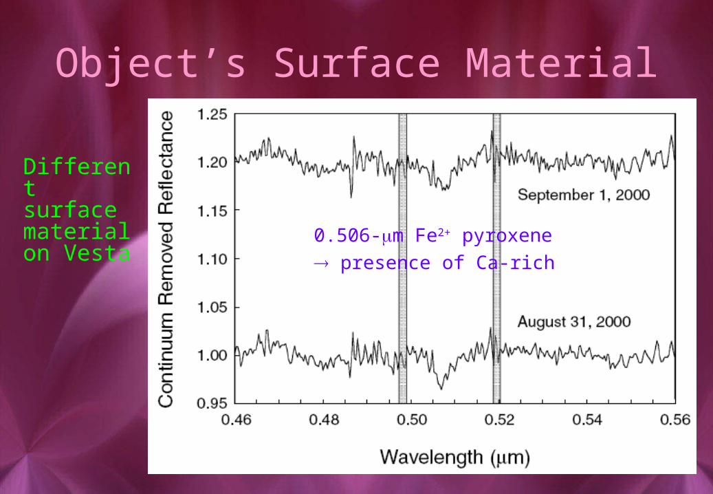
Object’s Surface Material

Different surface material on Vesta 0.506-m Fe2+ pyroxene

presence of Ca-rich

Effects of Surface Properties

• Phase reddening: reddening of reflectance spectra with increased phase angle

NIR Spectrometer to Eros: slope 8-12% over phase angles 0-100

• Space Weathering: darkening & reddening of asteroids’ surface

e.g. Chapman 1996: Explaining the spectral mismatches between asteroids and meteorites

• Particle size Particulate regolith on the surface• Temperature 120 K (Trojans) to >300 K (NEAs) Shapes of spectral bands (olivines & pyroxenes) are sensitive

to temperature

Taxonomy: methods• Asteroid classification Bowell et al. 1978 Tholen & Barucci 1989• Data sets: - ECAS (Zellner etl al. 1985) - IRAS albedo (Veeder et al. 1989, Tedesco et al. 1992)

Statistically significant boundaries exist between clusters of objects

1. Tholen taxonomy (1984): spanning tree clustering algorithm

2. Barucci et al. taxonomy (1987): G-mode analysis3. Tedesco et al. taxonomy (1989): visual identification of

groupings in a parameter space (two asteroid colors & IRAS albedo)

4. Howell et al taxonomy (1994): artificial neural network

• Tholen taxonomy was utilized in an attempt to preserve the historic structure and spirit of past asteroid taxonomies

• Classes were defined solely on the presence (or absence) of absorption features contained in the visible-wavelength spectra

• The classes were arranged in a way that reflects the spectral continuum revealed by the SMASSII data

• Different analytical and multivariate analysis technique were used to properly parameterize the various spectral features. Labels of some class were based on human judgment.

• When possible, the sizes (scale-lengths) and boundaries of the taxonomic classes were defined based on the spectral variance observed in natural groupings among the asteroids.

SMASSII Taxonomy: basicsBus et al. 2002

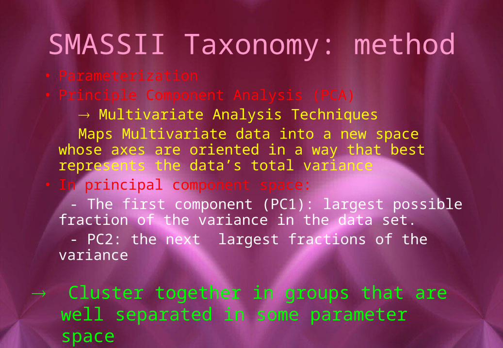
SMASSII Taxonomy: method• Parameterization• Principle Component Analysis (PCA) Multivariate Analysis Techniques Maps Multivariate data into a new space whose axes

are oriented in a way that best represents the data’s total variance

• In principal component space: - The first component (PC1): largest possible fraction

of the variance in the data set. - PC2: the next largest fractions of the variance

Cluster together in groups that are well separated in some parameter space

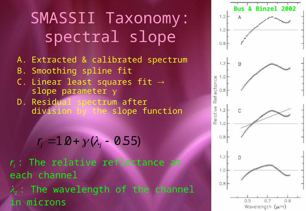
SMASSII Taxonomy: spectral slope

A. Extracted & calibrated spectrumB. Smoothing spline fitC. Linear least squares fit slope

parameter D. Residual spectrum after division by

the slope function

)55.0(0.1 iir

ri : The relative reflectance at each channel

I : The wavelength of the channel in microns

: The slope of the fitted line (unity at 0.55 m)

Bus & Binzel 2002

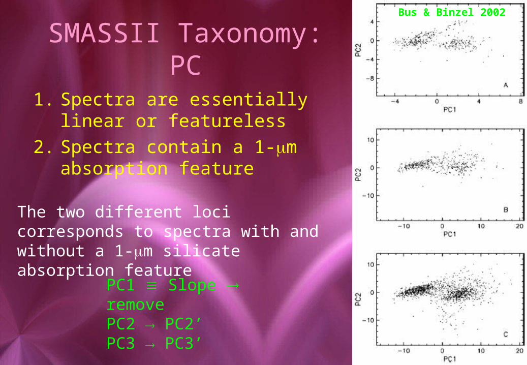
SMASSII Taxonomy: PC

1. Spectra are essentially linear or featureless

2. Spectra contain a 1-m absorption feature

The two different loci corresponds to spectra with and without a 1-m silicate absorption feature

PC1 Slope removePC2 PC2’PC3 PC3’

Bus & Binzel 2002

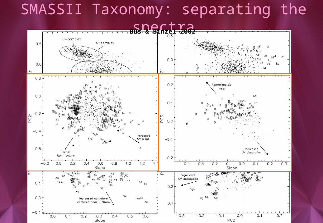
SMASSII Taxonomy: separating the spectraBus & Binzel 2002

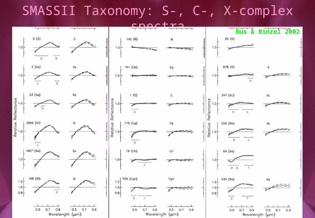
SMASSII Taxonomy: S-, C-, X-complex spectraBus & Binzel 2002

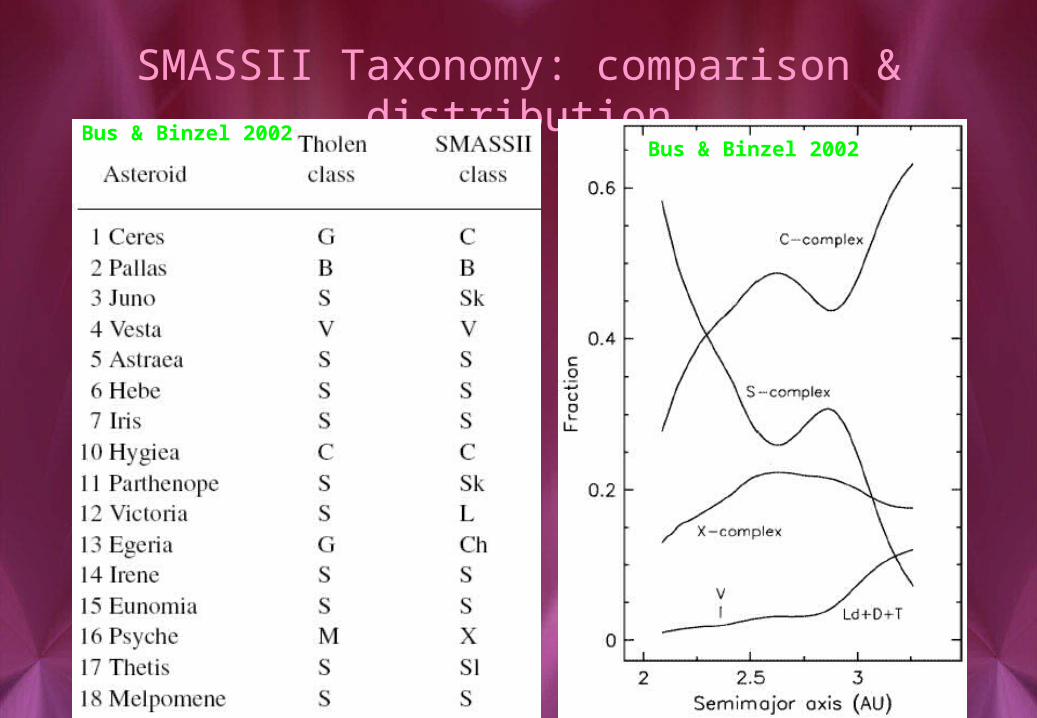
SMASSII Taxonomy: comparison & distributionBus & Binzel 2002

Bus & Binzel 2002

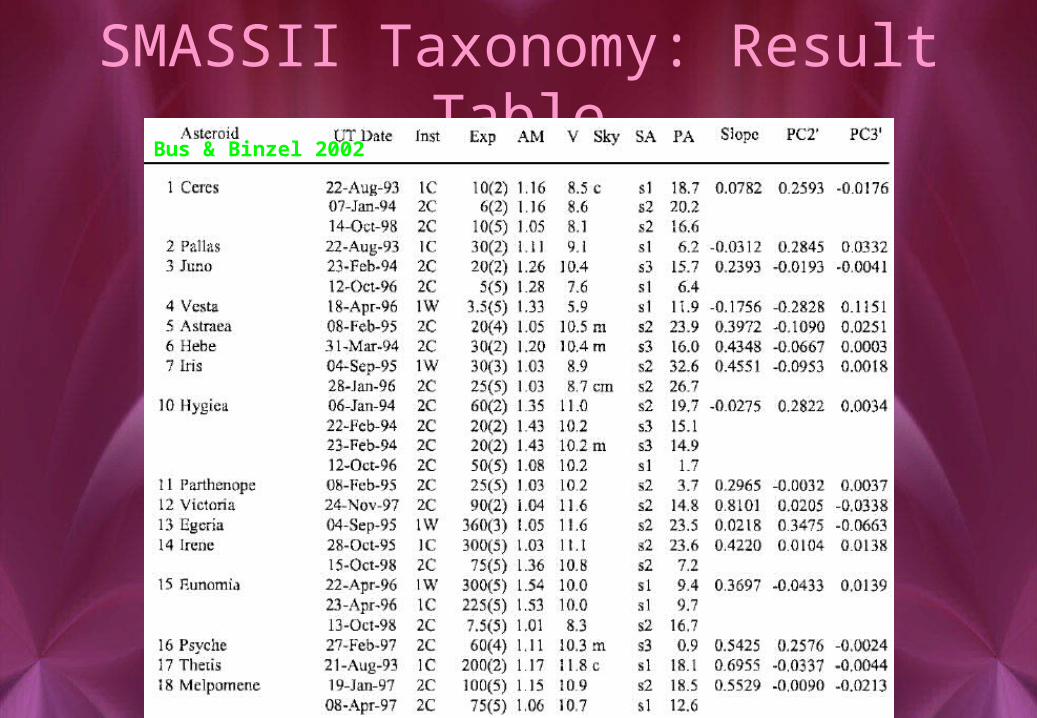
SMASSII Taxonomy: Result TableBus & Binzel 2002

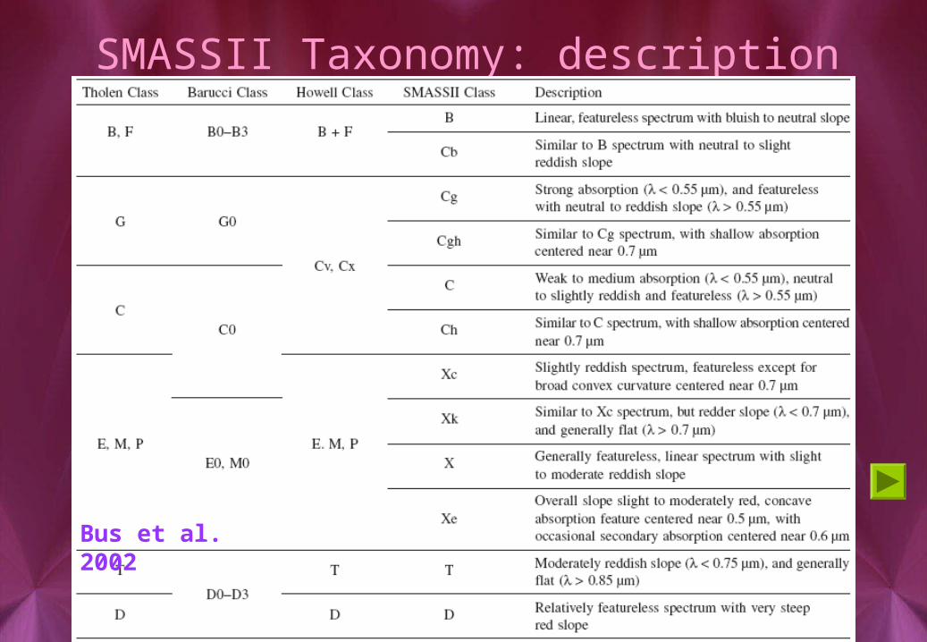
SMASSII Taxonomy: description

Bus et al. 2002

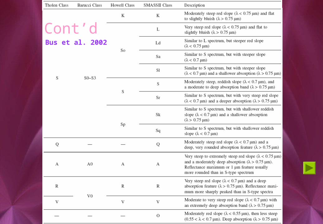
Cont’dBus et al. 2002

SMASSII Taxonomy: drawbacks

Can be cumbersome for newly observed asteroids

Allow for the classification of individual objects The classification assigned to an asteroid is

only as good as the observational data

Variations in spectrum may change the taxonomic label

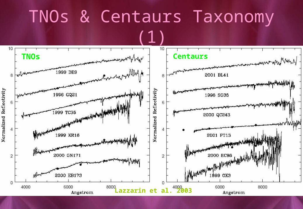
TNOs Centaurs

TNOs & Centaurs Taxonomy (1)

Lazzarin et al. 2003

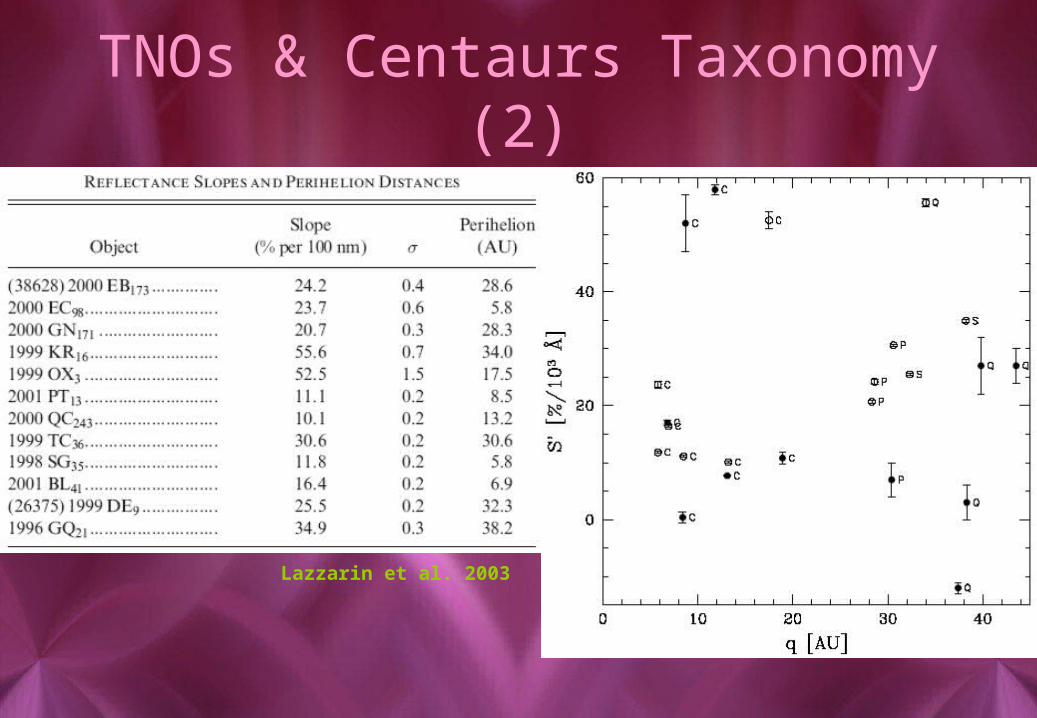
TNOs & Centaurs Taxonomy (2)

Lazzarin et al. 2003

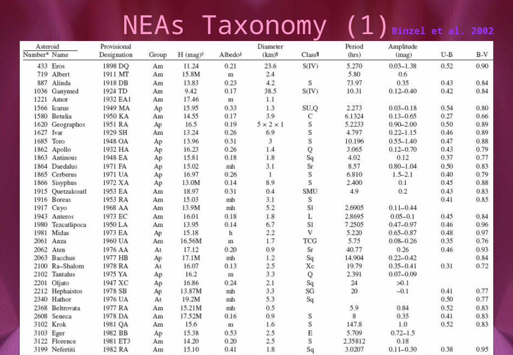
NEAs Taxonomy (1) Binzel et al. 2002

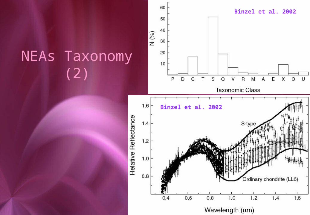
NEAs Taxonomy (2)

Binzel et al. 2002

Binzel et al. 2002

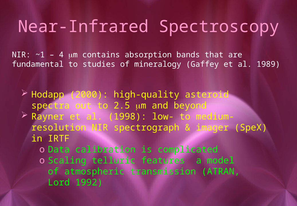
Near-Infrared Spectroscopy

NIR: ~1 – 4 m contains absorption bands that are fundamental to studies of mineralogy (Gaffey et al. 1989)

Hodapp (2000): high-quality asteroid spectra out to 2.5 m and beyond

Rayner et al. (1998): low- to medium-resolution NIR spectrograph & imager (SpeX) in IRTF

o Data calibration is complicatedo Scaling telluric features a model of atmospheric

transmission (ATRAN, Lord 1992)

Visible & NIR Spectroscopy

0.7 – 2.5 m: silicate minerals (pyroxenes, olivines and plagioclase)

Absorption bands near 1 & 2 m2.5 – 3.5 m: hydrated minerals (bound water

and structural OH)

Absorption bands centered near 3 m

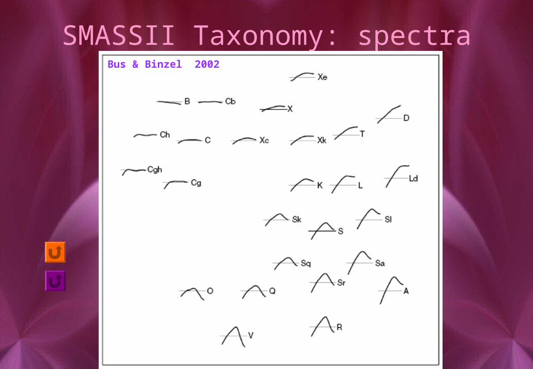
SMASSII Taxonomy: spectraBus & Binzel 2002