Taxes and Financing Decisions

Jonathan Lewellen* MIT and NBER

lewellen@mit.edu

Katharina Lewellen+

MIT klew@mit.edu

Revision: February 2005 First draft: June 2003

We are grateful to Nittai Bergman, Ian Cooper, Harry DeAngelo, Linda DeAngelo, Chris Hennessy, Dirk Jenter, Stew Myers, Jeff Pontiff, Jim Poterba, Josh Rauh, Toni Whited, and workshop participants at Baruch, Boston College, BYU, MIT, USC, UBC, Wisconsin, and the 2004 EFA and 2005 AFA meetings for helpful comments. We also thank Scott Weisbenner for providing data. * Sloan School of Management, 50 Memorial Drive, E52-436, Cambridge, MA 02142. + Sloan School of Management, 50 Memorial Drive, E52-435, Cambridge, MA 02142.

Taxes and Financing Decisions

Abstract

We argue that trade-off theory’s simple distinction between debt and ‘equity’ is fundamentally incomplete because firms have three, not two, distinct sources of funds: debt, internal equity, and external equity. Internal equity (retained earnings) is generally less costly than external equity for tax reasons, and may even be cheaper than debt. It follows that, without any information problems or adjustment costs, optimal leverage is a function of internal cashflows, debt ratios can wander around without a specific target, and a firm’s cost of capital depends on its mix of internal and external finance, not just its mix of debt and equity. The trade-off between debt, retained earnings, and external equity depends critically on the tax basis of investors’ shares relative to current price. We estimate how the trade off varies cross-sectionally and through time for a large sample of U.S. firms.

1. Introduction The finance literature has long offered a simple model of how taxes affect financing decisions, familiar to

generations of MBA students. Debt has tax advantages at the corporate level because interest payments

reduce the firm’s taxable income while dividends and share repurchases do not. Unless personal taxes

negate this advantage, interest ‘tax shields’ give corporations – that is, shareholders – a powerful

incentive to increase leverage.

The trade-off theory of capital structure is largely built upon the tax benefits of debt. In its simplest form,

trade-off theory says that firms balance the tax benefits of debt against the costs of financial distress.

(Leverage might also affect agency conflicts among stockholders, bondholders, and managers.) Tax

effects dominate at low leverage, while distress costs dominate at high leverage. The firm has an optimal,

or target, debt ratio at which the incremental value of tax shields from a small change in leverage exactly

offsets the incremental distress costs. This notion of a target debt ratio, determined by firm characteristics

like profitability and asset risk, is the central focus of most empirical tests (see, e.g., Shyam-Sunder and

Myers, 1999; Fama and French, 2002; Leary and Roberts, 2004).

This paper re-considers the tax effects of financing decisions in a simple yet, in important respects,

realistic model of taxation. Our main thesis is that, under general conditions, the tax costs of internal

equity (retained earnings) are less than the tax costs of external equity, and in principle may be zero or

negative. As a result, optimal leverage will depend on internal cashflows, debt ratios can wander around

without a specific target (much like in the pecking-order theory of Myers, 1984), and firms with excess

cash may not have a tax incentive to lever up. Further, the firm’s cost of capital depends on its mix of

internal and external finance, not just its mix of debt and equity. These predictions are all contrary to the

way trade-off theory is generally interpreted.

Our results follow from a simple observation whose importance for capital structure seems largely

unappreciated: when a firm distributes cash to shareholders, using either dividends or repurchases, the

payout triggers personal taxes that could otherwise be delayed. Thus, using internal cash for investment,

rather than paying it out to equityholders, has a tax advantage – the deferral of personal taxes – that

partially offsets the double-taxation costs of equity. An immediate implication is that internal equity is

less costly than external equity for tax reasons (i.e., both types of equity are subject to double taxation, but

only internal equity has the offsetting deferral effect).1

1 This observation isn’t new, but our results differ in important respects from related arguments in the literature. We discuss the literature below.

2

The tax-deferral benefit of retained earnings is well known, of course, but is typically discussed in the

context of payout policy, not capital structure. In a sense, our paper merges the two literatures: In the

capital structure literature, research focuses on the double-taxation costs of equity and generally ignores

the fact that distributions to shareholders (i.e., steps taken to reduce equity) accelerate personal taxes. The

opposite is true in the payout literature, which focuses on the tax-deferral benefit of retained earnings but

tends to ignore the double-taxation costs. We combine the two effects to evaluate the overall tax costs, or

benefits, of internal equity.

Our formal model quantifies these ideas when firms use either dividends or repurchases to distribute cash.

The general rule is that internal equity is less costly than external equity whenever distributions trigger

personal taxes, and, in principle, this effect can be large enough to completely offset the double-taxation

costs of equity (i.e., retained earnings may be better than debt financing). With dividends, the tax

advantage of internal equity depends on dividend and capital gains tax rates, τdv and τcg, as well as the

fraction α of capital gains that are realized and taxed each period. Intuitively, α determines how much

tax can be delayed if the firm decides to retain earnings: if α is zero, personal taxes are fully deferred if

the firm doesn’t pay dividends; if α is one, personal taxes must be paid, via either dividend or capital

gains taxes, regardless of the firm’s payout decision. We show that internal equity is less costly than

external equity as long as ατcg < τdv. If α is sufficiently small, internal equity may even be cheaper than

debt – that is, internal equity may have negative tax costs, even if tax rates are such that firms would

never want to raise external equity.

With repurchases, the tax advantage of internal over external equity depends on the tax basis on investors’

shares relative to the current price, a ratio we denote as β (endogenous in the model). Intuitively, β

determines how much tax is triggered by a share repurchase since it determines how much of the price

represents capital gains. If β is small, retaining cash inside the firm has a large tax deferral benefit;

internal equity is much less costly than external equity and, if β is sufficiently small, retained earnings can

even be better be better than debt. The cost of internal equity rises as β gets larger, and internal equity

becomes equivalent to external equity if β equals one.

We explore the implications of these results for capital structure, payout policy, and the cost of capital.

The main implications for capital structure are noted above: the tax advantage of internal over external

equity implies that optimal leverage is a function of internal cashflows and that firms have less incentive

to lever up than typically assumed (we show, in particular, that the trade-off between debt and retained

earnings depends on the capital gains tax rate, not the dividend tax rate, regardless of how the firm

3

distributes cash). The tax advantage of internal equity also implies that a firm’s cost of capital depends

on its mix of internal and external finance, not just its mix of debt and equity. The implication is that

firms’ investment decisions, like their capital structures, should depend on past profitability and

cashflows (see, also, Fazzari, Hubbard, and Petersen, 1988).

An important contribution of the paper is to show that subtle, often unstated, tax assumptions play a key

role in many capital structure theories. For example, Miller (1977) observes that, with personal taxes,

equity is preferred to debt if the after-tax return to shareholders on a dollar of corporate profits, (1 – τc)(1

– τe), is greater than the after-tax return to debtholders, (1 – τi) [τc, τi, and τe refer to the corporate tax rate

and the personal tax rates on interest and equity income]. In his analysis, Miller doesn’t differentiate

between internal and external equity, an assumption we show is valid only if α = 1 and the capital gains

tax rate equals the dividend tax rate. The first condition, α = 1, is equivalent to assuming that capital

gains are taxed on an ‘accrual’ basis.

Our analysis also relates to the growing literature on dynamic trade-off theory. This literature typically

focuses on the transaction costs associated with changing a firm’s capital structure, not the distinction

between internal and external equity (e.g., Fischer, Heinkel, and Zechner, 1989; Leland, 1998; Goldstein,

Ju, and Leland, 2001; Stebulaev, 2004). An important exception is Hennessy and Whited (2004), who

observe that substituting debt for internal cash has different tax consequences than substituting debt for

external equity, similar to the observation made here. A key difference is that Hennessy and Whited do

not account for capital gains taxes (shareholders pay tax only when they receive a cash distribution from

the firm). We show that their assumptions, in effect, maximize the tax advantage of internal over external

equity, which is a key source of dynamics in their model. Indeed, the difference between their results and

Miller (1977) is less that one is dynamic and the other static, but that the models implicitly make different

assumptions about taxes.

Our paper is perhaps closest to the public economics literature on dividend taxes. Like us, King (1974),

Auerbach (1979), and Bradford (1981) observe that retained earnings may be less costly than new equity

for tax reasons. We generalize their results to account for share repurchases and realization-based capital

gains taxes. In addition, Auerbach (1979) and Poterba and Summers (1985) discuss the so-called ‘trapped

equity’ view of dividends, which says that payout policy is irrelevant even with corporate and personal

taxes (in our language, the tax costs of internal equity are zero). We show that the trapped equity view is

precarious, holding only if tax rates are ‘just right.’ In fact, given the tax-on-accrual assumption standard

in this literature, internal equity has zero tax costs only if a Miller-like equilibrium holds, that is, only if

(1 – τc)(1 – τcg) = (1 – τi), where τcg is the capital gains tax rate.

4

Finally, our paper relates to Green and Hollifield (2003). Like us, they study how investors’ ability to

defer capital gains affects the cost of equity, and some of their results overlap with ideas in our paper.

The main difference is that they focus on valuation and the tax advantage of repurchases over dividends,

while we focus on the firms’ incentive to retain cash, the tax advantage of internal over external equity,

and the dynamics of capital structure through time.

The remainder of the paper is organized as follows. Section 2 presents a formal model of the tax costs of

debt, retained earnings, and external equity. Section 3 discusses the literature and Section 4 explores the

implications for corporate behavior. Section 5 estimates the tax costs of equity for a large sample of U.S.

corporations. Section 6 concludes.

2. Tax effects of financing decisions This section formalizes our arguments in a simple two-period model. (The model can be extended to

many periods; the crucial feature is that we have at least one intermediate date.) We incorporate realistic

tax assumptions, allowing the tax rates on dividends, capital gains, and interest income to differ and

recognizing that capital gains aren’t taxed until they are realized. Since our goal is to study the tax

consequences of financing decisions, not to develop a complete model of financing choice, we ignore

information asymmetries, agency conflicts, and distress costs. Thus, the model is in the spirit of

Modigliani and Miller (1963), Miller (1977), and Auerbach (1979).

Our main results concern the tax costs of internal equity and the dynamics of capital structure through

time. To make the ideas as transparent as possible, we start with a one-period model in which the firm

relies on external finance, and proceed to the two-period model in which the firm has internally-generated

earnings to reinvest in the second period.

2.1. One period The firm has an opportunity to invest I today in a project that pays I + P1, pre-tax, in one period. The

payoff can be random, but, to rule out bankruptcy, we assume that the rate of return is always more than

the riskless rate r (the connection to bankruptcy will be clear in a moment). Investors are risk neutral, and

both investors and the firm can invest in the riskless asset.

The firm initially has no cash but can sell debt and equity in competitive markets. We assume that any

cash raised must be invested inside the firm – that is, the firm can’t pay the cash immediately to

shareholders, leaving an empty shell. From this, and the fact that P1 > I r, debt is riskless because the firm

always has enough cash to repay debtholders.

5

Interest paid by the firm is tax deductible but dividends and repurchases are not. The corporate tax rate is

denoted τc and the personal tax rates on interest, dividends, and realized capital gains are denoted τi, τdv,

and τcg, respectively. With only one period, the firm is assumed to be liquidated at date 1, so all capital

gains are necessarily realized. The portion of a liquidating dividend that represents capital repayment is

exempt from personal taxes (consistent with the actual tax code).

In this model, it’s clear that capital structure conforms to the traditional debt-and-taxes story. Formally,

suppose the firm raises debt and equity of D0 and S0, with D0 + S0 ≥ I. Excess cash, C0 = D0 + S0 – I, is

invested in the riskless asset, so net income for the period is (P1 + C0 r – D0 r) (1 – τc). After paying

debtholders, the firm has cash at date 1 of

C1 = I + P1 (1 – τc) + (C0 – D0) [1 + r (1 – τc)]. (1) The last term in (1) implies that raising an extra dollar of debt to hold as cash has no effect on after-tax

income or cashflows, an observation we will return to later. Substituting for C0 yields

C1 = (P1 – I r) (1 – τc) + S0 [1 + r (1 – τc)]. (2) This equation says that every dollar of equity raises the firm’s cash holdings at date 1 by 1 + r (1 – τc).

The first term, which we denote as π1, is the firm’s after-tax income if it is entirely debt financed. The

firm distributes C1 as either a dividend or a repurchase, and the portion that represents capital repayment,

S0, is tax exempt in both cases. After personal taxes, shareholders receive

CF1 = π1 (1 – τe) + S0 [1 + r (1 – τc)(1 – τe)], (3) where τe denotes either τdv or τcg depending on whether dividends or repurchases are used. We assume

throughout the paper that τcg ≤ τdv, so repurchases are preferred. Equity is valuable if it yields a higher

after-tax payoff than investors can receive from holding the riskfree asset, 1 + r (1 – τi). Thus, the value

of equity financing relative to debt is

Net value of S0 at date 1 = S0 r [(1 – τc)(1 – τcg) – (1 – τi)], (4) assuming the firm disburses cash through a share repurchase (otherwise substitute τdv for τcg). These

results are all quite standard.

2.2. Two periods Our novel results come from adding a second period to the model (dates are numbered 0, 1, and 2). The

first period remains the same, but now the firm has the option either to pay cash to shareholders at date 1

or retain it until date 2. For simplicity, we assume the firm’s only investment opportunity at date 1 is the

6

riskfree asset; giving the firm a positive-NPV investment, like the project in the first period, only adds an

additional term to some of the expressions.

The firm can again sell debt and equity in competitive financial markets at dates 0 and 1. We assume for

convenience that debt is short term and, to prevent the possibility of bankruptcy, dividends at date 1 must

be paid before any new debt is issued (again, this prevents the firm from issuing debt and immediately

paying the proceeds to shareholders).

The tax treatment of dividends, repurchases, and capital gains becomes more important now that we have

multiple periods. Our assumptions attempt to match actual tax policy. In particular, we assume that

dividends are fully taxable but that repurchases are taxed only on the portion that represents capital gains.

Investors also pay capital gains tax on any remaining shares when they are sold, which means that we

have to make an assumption about trading behavior at date 1. A fully worked out model of trading is

obviously beyond the scope of the paper (tax incentives would imply zero trading). Our way of handling

the issue is to assume simply that investors trade an exogenous fraction α of their shares at date 1, which

thus represents the fraction of capital gains that are realized. We study how the results change as α varies

between zero and one.

Table 1 summarizes the firm’s cashflows. The first period remains exactly the same: net income is NI1 =

(P1 + C0 r – D0 r) (1 – τc) and cash on arrival to date 1, after repaying debt but before any other

transactions, is given by C1 in eq. (2). At date 1, the firm pays dividends or makes a share repurchase of

δ1 ≤ C1 and issues new debt and equity of D1 and S1. Cash on exit from date 1 is therefore C1′ = C1 + D1 +

S1 – δ1, which grows to

C2 = (C1′ – D1) [1 + r (1 – τc)] (5) at date 2, after taxes and debt payments. As we saw earlier, selling an extra dollar of debt to hold as cash

Table 1. The firm’s cashflows Date 0 Issue debt D0 and equity S0. Invest I in the project. Hold cash C0 = D0 + S0 – I ≥ 0. Date 1 Net income: NI1 = [P1 + C0 r – D0 r] (1 – τc) Cash on arrival, after taxes and debt: C1 = π1 + S0 [1 + r (1 – τc], where π1 = (P1 – I r) (1 – τc) Cash distribution δ1 Issue debt D1 and equity S1 Cash on exit: C1′ = C1 + S1 + D1 – δ1 ≥ 0 Date 2 Cash, after taxes and debt: C2 = [C1′ – D1] [1 + r (1 – τc)]

7

has no effect on the firm’s net income or cashflows. This observation gives our first result:

Proposition 1. Issuing debt to invest in the riskfree asset (i.e., to hold as cash) has no effect on shareholder value, regardless of tax rates.

Proposition 1 is fairly obvious and, we suspect, not really new (though we can’t cite a specific reference).

We highlight it for two main reasons. First, we believe it clarifies the connection between debt and taxes:

the right way to think about leverage is not that debt per se creates value, via interest tax shields, but that

equity potentially destroys value, via double taxation. Second, Proposition 1 simplifies our subsequent

analysis of equity financing: we can consider transactions between shareholders and the firm without

worrying about where the cash goes to or comes from. For example, the value of a dividend is the same

regardless of whether the firm draws down cash or increases borrowing, and it is the dividend payment

per se that affects value, not the possible debt transaction.

Equity financing

We now turn to equity financing at date 1. In the following, cash carried forward from the first to the

second period is referred to as ‘internal equity’ while new equity raised is ‘external equity.’ The ordering

of transactions affects the algebra, so we need to be more precise about timing in the model. We assume

that any cash payout at date 1 occurs before new equity is raised and that capital gains taxes at date 1 are

assessed before new equity is raised. These assumptions imply that external equity financing doesn’t

affect capital gains taxes at date 1, simplifying the algebra.2 Also, we initially assume that all cash

distributions are made via share repurchases – which are optimal from a tax standpoint – deferring for the

moment our analysis of dividends.

With these assumptions, external equity at date 1 has the same tax costs as external equity in the one-

period model. Substituting for C1′ in eq. (5), the firm’s cash at date 2 equals

C2 = (C1 + S1 – δ1) [1 + r (1 – τc)]. (6)

An extra dollar of external equity at date 1, S1, raises the firm’s cash holdings at date 2 by 1 + r (1 – τc).

If earnings are paid out through a share repurchase, this increases the after-tax cashflows to shareholders

by S1 [1 + r (1 – τc)(1 – τcg)], since the distribution is taxed only on the portion that represents capital

gains. As before, the tax costs depend on whether the return is higher or lower than the return from

investing directly in the riskless asset, 1 + r (1 – τi).

2 To clarify, suppose that equity financing is costly from a tax standpoint. Then any equity raised leads to an immediate capital loss, reducing taxes today but raising taxes later. We ignore this effect but, as discussed later, it is minor and does not significantly affect any results.

8

Proposition 2. When the firm uses repurchases, the tax benefit of external equity at date 1, or equival-ently, the net present value of a new equity issue, equals

PV(S1) = )]1()1)(1[()1(r1

rS icgci

1 ττττ

−−−−−+

. (7)

As mentioned above, Proposition 2 assumes that capital gains taxes at date 1 are assessed prior to the

equity issue. The present value of S1 would be attenuated slightly towards zero if we allowed the value

impact of S1 to feed immediately into capital gains.3 The key fact, however, is that the tax cost of external

equity still depends on whether equity taxes, (1 – τc)(1 – τcg), are higher or lower than debt taxes, (1 – τi),

just as in the one-period model.

The results so far match standard trade-off theory. The key differences arise when we consider internal

equity; indeed, trade-off theory doesn’t even distinguish internal from external equity except when

issuance costs are large (see, e.g., Fischer, Heinkel, and Zechner, 1989). We believe the easiest way to

understand the results is to compare the extreme cases when the firm either distributes all of its cash at

date 1 or retains all of it until date 2. Also, because external financing at date 1 doesn’t affect the value of

internal equity, we drop terms associated with S1 below.

The firm arrives at date 1 with cash C1. If the firm chooses to distribute the cash via a share repurchase,

equityholders receive

CF1, repurchase = C1 – τcg (C1 – S0). (8)

The second term reflects the fact that taxes are paid only on capital gains, C1 – S0. Shareholders get no

cash at date 2 in this scenario because the firm completely liquidates at date 1.

Alternatively, if the firm decides to retain all of its cash, shareholders don’t receive a distribution at date 1

but owe capital gains taxes of

CF1, retain = –α τcg (V1 – S0), (9)

where V1 is the equity value at date 1 before new equity is issued, derived below, and α represents the

fraction of capital gains that are realized and taxed. The tax basis of the shares is originally S0 at date 0,

but after trading it becomes:

TB1 = (1 – α) S0 + α V1. (10)

3 Eq. (7) would become

PV(S1) = )]1()1)(1[()1(r1

)1(rS icgc

cgi

cg1 τττ

αττατ

−−−−−−+

−.

The derivation of this equation closely parellels the algebra below for internal equity.

9

By date 2, the firm’s cash grows to C2 = C1 [1 + r (1 – τc)]. After personal taxes, shareholders receive

CF2, retain = C2 – τcg (C2 – TB1). (11)

Eq. (11) parellels eq. (8); it simply says that shareholders pay taxes only on the portion of the payout that

represents new capital gains. To determine V1, we assume that equity is valued at date 1 from the perspe-

ctive of current shareholders given the firm’s payout decision. V1 is therefore equal to the present value

of CF2,retain. In truth, V1 isn’t precisely pinned down because, with unrealized capital gains, existing

shareholders view the firm differently than would a new investor. The exact value isn’t critical to the

results – it has only a second-order effect – and the assumption that V1 equals the present value of eq. (11)

seems reasonable. Thus, V1 is given by

V1 = )1(r1

TB)1(r1)1(C

i

1cg

i

cg2

τ−+

τ+

τ−+

τ−. (12)

Define β as TB1 / V1, the ratio of the tax basis to price at date 1. Substituting for TB1 = β V1 and C2 = C1

[1 + r (1 – τc)], and solving for V1, yields

V1 = cgi

ccg1 )1(r1

)1(r1)1(Cβτ−τ−+

τ−+τ− . (13)

Together, eqs. (8) – (13) say that, if the firm retains all of its cash at date 1, shareholders receive no

immediate dividends, pay capital gains taxes of α τcg (V1 – S0) at date 1, and retain a claim worth V1.

Alternatively, shareholders could simply receive an immediate after-tax payout of C1 (1 – τcg) + τcgS0. The

tax benefit of internal equity is the difference between the present value of these two alternatives, which

gives the following result.

Proposition 3. The tax benefit of internal equity at date 1, or equivalently the present value of retained cash vis-à-vis a share repurchase, equals

PV(RE1) = )]1()1)(1[()1(r1

)1(rRE icgc

cgi

cg1 τβττ

βτττ

−−−−−−+

−, (14)

where RE1 is retained equity (equal to C1 if cash is fully retained) and β is the ratio of the tax basis of equity to current value at date 1.

Proposition 3 is one of our key results. It says that the tax costs of internal equity depend not only on

personal and corporate tax rates, as in traditional trade-off theory, but also on the tax basis of investors’

shares relative to current price, β = TB1 / V1. Intuitively, β determines how much additional tax is

triggered by a share repurchase. If β is low, a share repurchase accelerates the realization of large capital

gains which can otherwise be deferred, so retaining equity in the firm has a substantial tax benefit – the

10

deferral of personal taxes – that helps offset the tax costs of equity. Indeed, comparing Propositions 2 and

3, it’s clear that internal equity is always less costly than external equity if β < 1 and, if β is sufficiently

low, can actually have tax benefits (positive NPV).

Case 1: β = 0 The intuition for Proposition 3 is perhaps most transparent when the tax basis of investors’ shares is zero,

which requires that α and S0 are both zero. In this case, the PV of internal equity comes down to a simple

comparison: shareholders could either receive an after-tax payout at date 1 of C1 (1 – τcg), which they can

invest at a rate of 1 + r (1 – τi), or, if the firm chooses to retain the cash, shareholders could receive an

after-tax payout at date 2 of C1 [1 + r (1 – τc)] (1 – τcg). The main benefit of paying cash to shareholders

today, and allowing them to invest directly in the riskfree asset, is that future interest income is taxed only

at the personal level; the main cost is that shareholders are forced to pay taxes immediately on first-period

earnings. These effects exactly offset when personal and corporate tax rates are the same. More

generally, when β = 0, Proposition 3 simplifies to:

PV(RE1) = )]1()1[()1(r1

)1(rRE ic

i

cg1 τ−−τ−

τ−+

τ−. (15)

The sign of eq. (15) depends solely on whether cash held inside or outside the firm earns a higher after-

tax interest rate (1 – τc vs. 1 – τi). The double taxation of equity drops out because it is, in essence, a sunk

cost: if τi = τc, the present value of taxes is the same regardless of whether the firm pays out cash today or

tomorrow, and regardless of the capital gains tax rate.

Case 2: β = 1 The case above, β = 0, maximizes the tax benefits of internal equity. Intuitively, β determines how much

tax is triggered by a share repurchase or, equivalently, deferred until date 2 by retaining cash inside the

firm. The deferral benefit drops as β gets larger and vanishes when β equals one since, in that case, no

part of the purchase price represents capital gains. From eq. (10), β = 1 only if α = 1 – that is, only if all

capital gains are taxed immediately regardless of the firm’s payout decision, so that the tax basis equals

the current price. Internal and external equity in this case become essentially equivalent. Proposition 3

simplifies to:

PV(RE1) = )]1()1)(1[()1(r1

)1(rRE icgc

cgi

cg1 τ−−τ−τ−

τ−τ−+

τ−

11

≈ )]1()1)(1[()1(r1

rRE icgci

1 τ−−τ−τ−τ−+

. (16)

The second line is a close approximation to the first if tax rates aren’t too big. It is identical to the tax

cost of external equity given in Proposition 2.4

Thus, internal and external equity are the same, and the tax cost of both is given by eq. (16), only when

capital gains are taxed on accrual, i.e., when α = β = 1. This assumption is implicit in Miller (1977) and

in the standard interpretation of trade-off theory. The tax costs of internal equity are always smaller if β

is less than one, and might well be negative even when external equity is costly. In fact, if β is less than

one and a Miller equilibrium holds for external equity, (1 – τc)(1 – τcg) = (1 – τi), Proposition 3 implies

that internal equity necessarily has tax benefits.

Dividends We’ll discuss Proposition 3 further in a moment, but it’s useful to consider first how the results change if

dividends are used instead of repurchases. The motivation for doing so is two-fold. First, firms do use

dividends in practice, despite their clear tax disadvantages. Second, the tax literature often assumes that

firms have to use dividends for regulatory or agency reasons, so understanding the tax costs of equity

when dividends are used allows an easier comparison with prior studies (e.g., King, 1974; Auerbach,

1979; Poterba and Summers, 1985).

The algebra for dividends is similar to that for repurchases; the main difference is that the entire distribu-

tion is taxable. We assume that dividends cannot be more than cumulative net income and, at date 2, cash

remaining after dividends (equal to contributed capital) is disbursed through a share repurchase. Our

analysis again compares the extremes, when the firm either pays a dividend at date 1 equal to first-period

earnings or fully retains the cash until date 2.

The firm arrives at date 1 with cash C1 = NI1 + S0. If the firm chooses to pay dividends equal to NI1,

shareholders’ cashflow at date 1 is

CF1,div = NI1 (1 – τdv) – α τcg (V1,div – S0). (17)

The first term is the after-tax dividend and the second term is capital gains tax (V1,div is equity value after

4 The small difference in the first line arises because the value implications of retained earnings feed immediately into capital gains taxes at date 1, while the value implications of external equity do not; see our discussion prior to Proposition 2. If internal and external equity are treated the same, the tax costs would be identical when α = β = 1 (compare the expression in eq. 16 to the expression in footnote 3 when α = 1).

12

the dividend payment, derived in a moment). The new tax basis of equity becomes TB1 = S0 + α (V1,div –

S0). At date 2, the firm’s cash holdings grow to S0 [1 + r (1 – τc)], of which S0 r (1 – τc) represents net

income that is paid out as a dividend and the remainder, S0, is paid out as a liquidating repurchase. Share-

holders receive, after taxes, the following at date 2:

CF2, div = S0 [1 + r (1 – τc)(1 – τdv)] + α τcg (V1,div – S0). (18)

V1,div is determined by the present value (at date 1) of CF2,div, and the total value of equity at date 1 is the

sum of V1,div and CF1,div.

Alternatively, the firm can choose to retain cash until date 2. In this case, shareholders don’t receive a

dividend at date 1 but owe capital gains taxes of

CF1,retain = –α τcg (V1,retain – S0). (19)

At date 2, the firm’s cash holdings grow to C2 = C1 [1 + r (1 – τc)] = (NI1 + S0) [1 + r (1 – τc)], of which

NI1 + (NI1 + S0) r (1 – τc) represents cumulative earnings, paid out as a dividend, and the remainder S0 is

paid out as a liquidating repurchase. After personal taxes, shareholders receive

CF2,retain = NI1(1 – τdv)[1 + r (1 – τc)] + S0 [1 + r (1 – τc)(1 – τdv)] + α τcg (V1,retain – S0). (20)

Again, V1,retain is found as the present value of eq. (20), and the total value of equity is the sum of V1,retain

and CF1,retain. The tax benefit of internal equity is then just the difference between the present value of the

two alternative policies, paying a dividend today vs. retaining the cash until date 2. After some algebra,

we have the following result.

Proposition 4. When the firm uses dividends, the tax benefit of internal equity at date 1 (or equivalently the present value of retained earnings vis-à-vis dividends) equals

PV(RE1) = )]1()1)(1[()1(r1

)1(rRE icgccgi

dv1 ταττ

ατττ

−−−−−−+

− , (21)

where RE1 is retained earnings (equal to NI1 if earnings are fully retained) and α is the fraction of capital gains taxed at date 1.

Proposition 4 differs from Proposition 3 in two respects. First, the numerator contains 1 – τdv rather than

1 – τcg because distributions are now taxed at the dividend rate. Second, the term in brackets depends on

α, not β. Intuitively, when repurchases are used, the ratio of the tax basis to current price, β, determines

how much tax is triggered today by a repurchase (and how much is deferred by retaining cash). But α

plays this role when dividends are used: the entire distribution is taxed if the firm pays dividends, but

only a fraction α is taxed, via capital gains, if the firm chooses to retain cash.

13

It is important that the capital gains tax rate, not the dividend tax rate, appears in the term in brackets.

Even when the firm uses dividends, the cost of internal equity depends on whether (1 – τc)(1 – ατcg) is

bigger than or less than (1 – τi). The after-tax rate on dividends, 1 – τdv enters eq. (21) only multipli-

catively, so does not determine whether internal equity is better than debt. [Auerbach (1979) shows a

similar result for the special case when α = 1.] Intuitively, dividend taxes are a sunk cost regardless of

the payout decision, and the present value of retained earnings depends solely (in sign, not magnitude) on

capital gains taxes. This result is worth repeating: the cost of internal equity depends primarily on the

capital gains tax rate even when firms use dividends.

Our earlier analysis of external equity assumed that firms use share repurchases. When dividends are

used, Proposition 2 changes only by the substitution of τdv for τcg in the term in brackets:

PV(S1) = )]1()1)(1[()1(r1

rS idvci

1 τ−−τ−τ−τ−+

. (22)

This equation ignores the immediate effect of S1 on capital gains taxes, as discussed previously. If we

take that effect into account, the cost of external equity becomes

PV(S1) = )]1()1)(1[()1(r1

)1(rS idvc

cgi

cg1 τ−−τ−τ−

ατ−τ−+

ατ−. (23)

Comparing this to Proposition 4, internal equity is less costly than external equity if ατcg < τdv, which of

course holds as long as τcg < τdiv. [King (1974) and Auerbach (1979) show a similar result for α = 1.]

Thus, dividends don’t change our key qualitative conclusion: internal equity is less costly than external

equity, regardless of whether the firm uses dividends or repurchases. If α and/or β is sufficiently low,

firms might actually prefer internal equity over debt, even when tax rates are such that they would never

want to raise external equity financing.

3. Understanding the literature

The results above have significant implications for a firm’s capital structure, payout policy, and cost of

capital. The model also clarifies a number of prior studies. We discuss the literature first because it

shapes the way we think about taxes and financing decisions.

Most clearly, our results show that the traditional view of debt and taxes, as exemplified by Miller (1977),

is valid only when capital gains are taxed on accrual, i.e., when α = β = 1. The main features of the

traditional view are (i) internal and external equity are assumed to be equivalent, and (ii) the tax cost of

14

equity depends on the total taxation of equity relative to debt, (1 – τc)(1 – τe) – (1 – τi). The first

statement is generally false and the second is, at best, incomplete (it misses the distinction between

internal and external equity and it is unclear about τe).

Like Miller, dynamic trade-off models generally don’t distinguish between internal and external equity

(Fischer, Heinkel, and Zechner, 1989; Leland, 1998; Goldstein, Ju, and Leland, 2001; Stebulaev, 2004).

Capital structure dynamics in the models are driven by agency problems and adjustment costs – the focus

of the studies – not by a tax advantage of internal over external equity. The literature sometimes

acknowledges that, because capital gains are not taxed until they are realized, the effective tax rate on

capital gains is less than the statutory rate. But simply allowing for a low effective tax rate isn’t sufficient

because it misses the differential tax costs of internal and external equity.

In an important recent paper, Hennessy and Whited (2004) present a dynamic model that deviates from

the characterization above. Their model allows for personal taxes and, unlike most dynamic theories, it

recognizes that retained earnings have different tax effects than new equity financing. For example,

Hennessy and Whited argue that debt is more attractive when it substitutes for external equity than when

it finances distributions to shareholders, an observation similar to our point that internal equity is less

costly than external equity. Because of this similarity and the rather intimidating nature of Hennessy and

Whited’s dynamic model, it is useful to consider their results more closely. (The following comments

also apply to the related analysis of Stiglitz, 1973.)

It turns out that Hennessy and Whited make two key assumptions: (i) investors do not pay capital gains

taxes, and (ii) firms implicitly cannot use share repurchases. The tax effects of retained earnings in their

model seem to be a special case of Proposition 4 when either α or τcg is zero (though an exact comparison

is hard because of the model’s complexity). The stylized examples in their Section I illustrate this point

nicely: investors don’t pay capital gains tax in any of the examples and retained earnings are beneficial if

τc < τi, the same conclusion from Proposition 4 when α = 0. Hennessy and Whited effectively make the

same assumptions in their formal dynamic model: shareholders pay tax on the entire amount of any cash

distribution and they otherwise pay no capital gains taxes. These assumptions can be satisfied only if the

firm uses dividends and either α or τcg is zero.

We believe that Hennessy and Whited’s predictions would change substantially if they accounted for

capital gains taxes. In particular, the assumption that ατcg = 0 maximizes the tax advantage of internal

equity, which is a key source of dynamics in their model. Indeed, our results suggest that, ignoring other

considerations like flotation costs, Hennessy and Whited’s model might well predict a stable, target debt

15

ratio if it made the same tax-on-accrual assumption implicit in Miller (1977) (if it did, internal and

external equity would become equivalent as long as firms can use share repurchases to distribute cash).

We hasten to add, however, that we don’t regard the tax-on-accrual assumption as empirically valid (we

provide evidence later). Our point is simply that assumptions about capital gains taxes are critical for

understanding their results.

Our paper also relates to the large public economics literature on dividend taxes. King (1974), Auerbach

(1979), Bradford (1981), and Poterba and Summers (1985) study how corporate and personal taxes affect

valuation and firms’ real investment decisions (Auerbach, 2002, provides a recent survey). Their infinite-

period models are similar in spirit to ours, and, like us, they observe that retained earnings are less costly

than new equity. [The implications of that result, however, are overlooked by the capital structure

literature; see, e.g., Graham’s (2003) recent survey.] The main difference with our results in that King et

al. assume that firms have to use dividends and that capital gains are taxed on accrual; thus, their results

are a special case of Proposition 4 with α = 1.

The focus of much of the dividend tax literature – see, in particular, Auerbach (1979) and Poterba and

Summers (1985) – is on the ‘tax capitalization’ or ‘trapped equity’ view of dividends. This view says

that, if firms are prohibited from using share repurchases, payout policy turns out to be irrelevant: in

equilibrium, shareholder wealth doesn’t change if the firm retains a dollar of earnings vs. pays a dollar of

dividends because the present value of taxes is the same in both cases. (In our language, the notion of

‘trapped’ equity is equivalent to saying that internal equity has zero tax costs.) This view is important

because, as Auerbach and Poterba and Summers explain, it has powerful implications for tax policy: if

the trapped equity view is accurate, dividend taxes will affect a firm’s value but not its cost of capital or

investment decisions.

Our results provide an easy way to understand the trapped equity view – and to see that it holds only in

special circumstances. From Proposition 4, shareholders are indifferent between dividends and retained

earnings only if tax rates are ‘just right,’ i.e., only if (1 – τc)(1 – ατcg) = (1 – τi).5 Our model does,

however, confirm the trapped equity prediction about real investment decisions: we show below that, as a

general rule, dividend taxes do not affect the cost of capital for internal equity.

5 The tax literature often assumes accrual taxation, in which case dividend policy is irrelevant only if (1 – τc)(1 – τcg) = (1 – τi). This fact is actually imbedded, though not obvious, in Auerbach’s (1979) model. Poterba and Summers (1985) consider a firm that is all-equity financed, so τi doesn’t enter their analysis; their version of ‘trapped equity’ requires that the firm always has enough internal cashflow to cover investments, that it has to use dividends rather than repurchases, and that it cannot raise debt.

16

4. Implications for corporate behavior

The analysis above establishes two key results. First, internal equity is generally less costly than external

equity. Second, the tax costs of internal equity depend on α and β, which determine how much tax is

triggered by a payout to shareholders. The results have significant implications for thinking about capital

structure, payout policy, and the cost of capital.

4.1. Capital structure

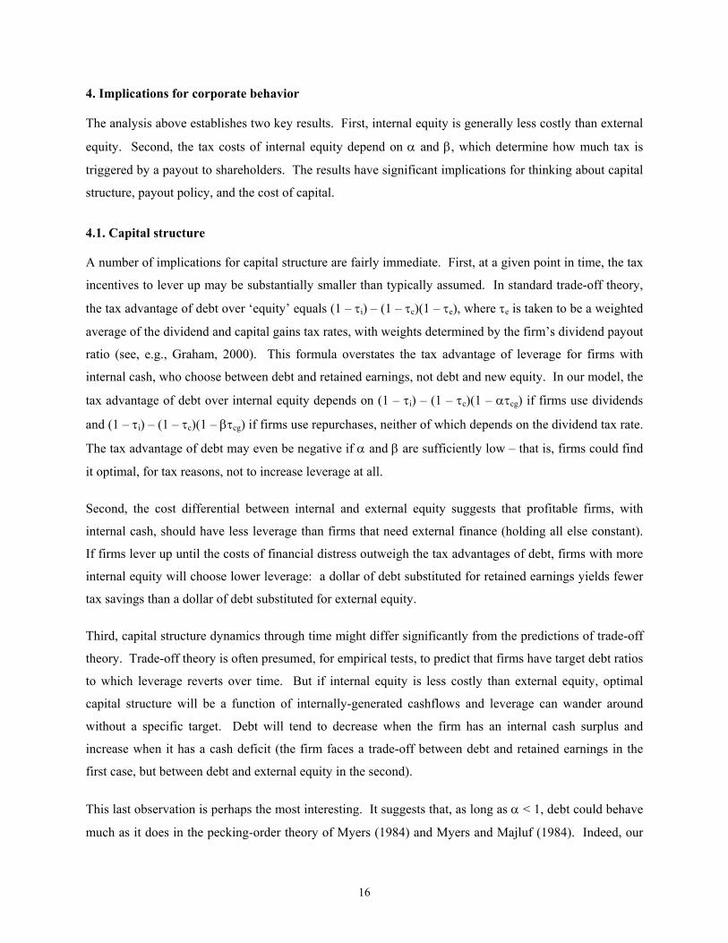
A number of implications for capital structure are fairly immediate. First, at a given point in time, the tax

incentives to lever up may be substantially smaller than typically assumed. In standard trade-off theory,

the tax advantage of debt over ‘equity’ equals (1 – τi) – (1 – τc)(1 – τe), where τe is taken to be a weighted

average of the dividend and capital gains tax rates, with weights determined by the firm’s dividend payout

ratio (see, e.g., Graham, 2000). This formula overstates the tax advantage of leverage for firms with

internal cash, who choose between debt and retained earnings, not debt and new equity. In our model, the

tax advantage of debt over internal equity depends on (1 – τi) – (1 – τc)(1 – ατcg) if firms use dividends

and (1 – τi) – (1 – τc)(1 – βτcg) if firms use repurchases, neither of which depends on the dividend tax rate.

The tax advantage of debt may even be negative if α and β are sufficiently low – that is, firms could find

it optimal, for tax reasons, not to increase leverage at all.

Second, the cost differential between internal and external equity suggests that profitable firms, with

internal cash, should have less leverage than firms that need external finance (holding all else constant).

If firms lever up until the costs of financial distress outweigh the tax advantages of debt, firms with more

internal equity will choose lower leverage: a dollar of debt substituted for retained earnings yields fewer

tax savings than a dollar of debt substituted for external equity.

Third, capital structure dynamics through time might differ significantly from the predictions of trade-off

theory. Trade-off theory is often presumed, for empirical tests, to predict that firms have target debt ratios

to which leverage reverts over time. But if internal equity is less costly than external equity, optimal

capital structure will be a function of internally-generated cashflows and leverage can wander around

without a specific target. Debt will tend to decrease when the firm has an internal cash surplus and

increase when it has a cash deficit (the firm faces a trade-off between debt and retained earnings in the

first case, but between debt and external equity in the second).

This last observation is perhaps the most interesting. It suggests that, as long as α < 1, debt could behave

much as it does in the pecking-order theory of Myers (1984) and Myers and Majluf (1984). Indeed, our

17

model suggests a kind of tax-induced pecking order, with debt and internal equity both preferred to

external equity (the ordering of debt and internal equity is ambiguous and could change over time, for

example, as a function of current leverage). Thus, our model might help explain two findings that have

been described as ‘major failures’ of trade-off theory: (i) profitable firms seem to have too little leverage,

and (ii) changes in debt largely absorb short-run variation in internal cash surpluses and deficits (e.g.,

Shyam-Sunder and Myers, 1999; Fama and French, 2002).

4.2. Payout policy

The model’s implications for payout policy stem, in large part, from the observations above. The model

is particularly helpful for understanding the so-called ‘dividend puzzle,’ the view that paying dividends is

suboptimal from a tax standpoint. One version of this view says that dividends destroy value because, if

firms chose to retain the cash instead, investors could convert highly-taxed dividends into less highly-

taxed capital gains (Black, 1976; DeAngelo, 1991; DeAngelo and DeAngelo, 2004). The inference seems

to be that retained earnings are preferred if τcg < τdv.

However, if the argument is simply about the timing of a payout – dividends will be paid sometime just

not necessarily this year – taxes provide an incentive to delay dividends only if internal equity is better

than debt, i.e., only if (1 – τc)(1 – ατcg) > (1 – τi).6 The relative tax rates of dividends and capital gains

aren’t at all important. Further, what we perceive as two commonly held beliefs, that debt levels are too

low for profitable firms (with excess cash) and that dividends destroy value for tax reasons, are logically

inconsistent with each other: the first says that firms should distribute cash (and raise debt), the second

says they should not. Also, if a Miller-like equilibrium holds with respect to internal equity, then we are

back to Auerbach’s (1979) trapped-equity view: on the margin a dollar of retained earnings is worth the

same as a dollar of dividends, so there is no dividend puzzle.

The dividend puzzle is more accurately a statement about the form of a cash payout; i.e., given that a

payout takes place, repurchases are clearly preferred to dividends (except, perhaps, if τcg > τdv; this is both

intuitive and easily shown in our model). Our results do nothing to explain why firms use dividends

rather than share repurchases.

As an aside, the model suggests that past financing decisions might affect current payout policy. From

6 This statement assumes that the firm has excess cash now and in the future (dividends today reduce dividends tomorrow). The incentive to retain cash is higher if external equity might be needed someday. For example, if as a consequence of paying dividends today, the firm might have to raise new equity in a year, then it would have to weigh the tax advantage of internal over external equity (in a year) against the one-year cost of holding cash. Hennessy and Whited (2004) explore this trade-off more formally.

18

Proposition 3, the tax benefits of internal equity vis-à-vis share repurchases are a decreasing function of β,

the tax basis of equity relative to current price:

PV(RE1) = )]1()1)(1[()1(r1

)1(rRE icgc

cgi

cg1 τ−−βτ−τ−

βτ−τ−+τ−

. (25)

Equity financing at date 0 raises the tax basis of investors’ shares, which, in turn, raises the tax costs (or

reduces the benefits) of retained earnings at date 1. Thus, past equity issues tend to make repurchases

more attractive relative to retaining the cash.

4.3. Cost of capital

The traditional view of a firm’s cost of capital is fairly straightforward. According to trade-off theory, a

firm’s cost of capital is a weighted average of the after-tax cost of debt and the cost of equity. The

relative weighting of the two is generally assumed to be fairly constant, consistent with the notion that the

firm has a target debt ratio.

Our model shows that this view is incomplete. Most important, a firm’s cost of capital should depend not

only on a firm’s mix of debt and equity, but also on its mix of internal and external finance: the tax

advantage of internal equity implies that a firm will accept projects with lower returns if they can be

financed with retained earnings rather than new equity. In our model, it is easy to show that the cost of

internal equity, expressed as a required return, is r (1 – τi) / (1 – ατcg) if the firm uses dividends and r (1 –

τi) / (1 – βτcg) if the firm uses repurchases; the cost of external equity in the first case is r (1 – τi) / (1 – τdv)

and in the second is r (1 – τi) / (1 – τcg). [The cost of capital is the minimum return, after corporate taxes,

that the firm requires on a project depending on how it is financed; the cost of debt is simply r (1 – τc), the

after-tax return on the riskless asset.] Thus, regardless of whether the firm uses dividends or repurchases,

the cost of internal equity is generally lower than the cost of external equity, an observation missed by

traditional trade-off theory. It is also important that the cost of capital for internal equity doesn’t depend

on the dividend tax rate, as we noted earlier.

Stepping a bit outside our model, it isn’t at all clear how the cost of internal or external equity relates to

the expected return on a firm’s stock. The standard way to determine a firm’s cost of equity is to estimate

the rate of return required by investors in the stock market. However, without going into the details, the

discount rate implied by equity prices in our model doesn’t have to equal either the cost of internal or

external equity shown above – that is, as a general rule, the expected stock return doesn’t equal the cost of

equity financing. A full analysis of these effects is beyond the scope of the paper. In practice,

19

quantifying them precisely is likely to be difficult because we would need to know not only the marginal

source of funds today (internal vs. external equity), but also how investments made today affect the

marginal source of funds in the future.

A corollary to these arguments is that investment decisions should depend on a firm’s internal cashflow.

That is, the advantage of internal equity implies that the firm’s investment-to-cashflow sensitivity should

be positive, consistent with empirical evidence (see, e.g., Fazzari, Hubbard, and Petersen, 1988; Hoshi,

Kashyap, and Scharfstein, 1991). The size of this effect will depend on whether the firm uses dividends

or repurchases, on corporate and personal taxes, and on the parameters α and β. (Fazzari et al. also

observe that taxes might lead to a positive investment-to-cashflow sensitivity; their analysis is based on

Auerbach’s (1979) model.) In short, our results imply that cost of capital is more complex than suggested

by the traditional trade-off model.

5. Tax costs of equity: Empirical evidence Our results show that the cost of internal equity depends on α, the fraction of capital gains that are

realized and taxed each period, and β, the tax basis of investors’ shares relative to current price. This

section provides estimates of α, β, and the tax costs of equity for a large sample of U.S. corporations from

1966 – 2003. For simplicity, we estimate the parameters for a representative investor who faces typical

tax rates on dividends, capital gains, and interest income, and who’s tax basis corresponds to the average

tax basis of all shareholders. We allow tax rates to change through time to match the historical

experience of U.S. investors.

5.1. Tax rates Figure 1 on the next page shows estimates of marginal tax rates from 1966 – 2003. The corporate tax

rates, from Poterba (2004, Table A.5), represent the top marginal tax rate on corporate income in each

year. The personal tax rates, from the National Bureau of Economic Research (www.nber.org/taxsim),

represent dollar-weighted average marginal tax rates on interest, dividends, and realized long-term capital

gains for a large sample of U.S. taxpayers. The rates are estimated by NBER’s TAXSIM model, as

described by Feenberg and Coutts (1993).

5.2. Estimating the tax basis The costs of internal equity depend not only on corporate and personal tax rates, but also on the tax basis

of investors’ shares relative to current price. While the tax basis isn’t directly observable, we can get an

estimate using price and volume data for each firm. As described below, we construct several measures

20

based on different assumptions about trading behavior.

Proportional trading In the simplest case, we assume that all investors holding a stock are equally likely to trade, regardless of

when they purchased their shares (similar to Grinblatt and Han, 2001). This assumption allows us to

recursively estimate the firm’s tax basis using observed trading volume (and given an estimate of the

beginning tax basis). For example, if the tax basis at the beginning of trading is TB0, then

TB1 = v1 P1 + (1 – v1) TB0 TB2 = v2 P2 + (1 – v2) TB1 = v2 P2 + (1 – v2) v1 P1 + (1 – v2)(1 – v1) TB0 TB3 = v3 P3 + (1 – v3) TB2 = v3 P3 + (1 – v3) v2 P2 + (1 – v3)(1 – v2) v1 P1 + (1 – v3)(1 – v2)(1 – v1) TB0, where Pt and vt are price and trading volume on date t. The logic is that vt shares are purchased on date t

but then a fraction vt+k are sold on each subsequent date. As a result, the tax basis evolves according to

TBt = vt Pt + (1 – vt) TBt-1. Recursively substituting for TBt-i, the tax basis is a weighted average of past

prices where the weights are given by

∏−

= −−− −=

1i

0j jtitit

t )v1(vw . (26)

In principle, the starting tax basis, TB0, should be the average price at which equity is contributed prior to

and at the IPO. Since that isn’t publicly available, we try two possible assumptions (it’s useful to note,

too, that TB0 becomes less important as trading progresses). A conservative guess – conservative in the

sense that is minimizes the tax advantage of internal equity – is to set TB0 equal to the first observed

0%

10%

20%

30%

40%

50%

60%

1966 1969 1972 1975 1978 1981 1984 1987 1990 1993 1996 1999 2002

CorporateDividendInterestLT cap gain

Figure 1. Corporate and personal tax rates, 1966 – 2003 The figure shows the top marginal corporate tax rate and estimates of average marginal personal tax rates oninterest, dividends, and realized long-term capital gains. The corporate rates come from Poterba (2004) and thepersonal rates come from NBER’s TAXSIM model.

21

price. This price almost certainly overstates TB0 by a considerable margin since firms are both under-

priced at the IPO and go public after being successful. Our second assumption, therefore, sets TB0 equal

to one-half the first trading price.

IPW hazard rates The algorithm above assumes that trading volume is as likely to come from investors who bought

yesterday as from those who bought, say, five years ago. This assumption provides a useful benchmark

but probably isn’t accurate: Ivković, Poterba, and Weisbenner (IPW; 2004) show that investors are much

more likely to sell if they recently bought than if they’ve already held for many months. More

specifically, they estimate investors’ propensity to sell as a function of how long they’ve owned the stock

for a large sample of individual investors. The hazard rate, i.e., the probability of a sale in a given month

conditional on holding the stock up to that time, is 15% for the first month, declines to less than 4% by

month 6, and drops to about 1% by month 35. The hazard rates and the cumulative probability of a sale

within t months are shown in Figure 2.

We use IPW’s hazard rates to obtain three additional estimates of the tax basis. For the first estimate, we

assume that investors trade exactly as predicted by IPW’s hazard rates (and that shareholders at the IPO

act as if they just bought the shares). Accordingly, trading volume should evolve as follows:

v1′ = h1 v2′ = h1 v1′ + h2 (1 – v1′) v3′ = h1 v2′ + h2 (1 – h1) v1′ + h3 (1 – h2) (1 – v1′),

0%

10%

20%

30%

40%

50%

60%

70%

1 4 7 10 13 16 19 22 25 28 31 34Month after buying

Cumulative prob. of sale

Hazard rate

Figure 2. Holding periods and trading probabilities The graph shows (i) the probability that an individual investor sells in month t conditional on having held the stockfor t-1 months (the hazard rate), and (ii) the cumulative probabilty of a sale within the first t months. Source:Ivković, Poterba, and Weisbenner (2004).

22

where hi is the IPW hazard rate for an investor who still holds after i-1 months. Continuing the sequence,

trading volume would eventually converge to a steady state value determined by the hi (we assume that

the hazard-rate curve is flat after month 36). The pattern of hi also determines the fraction of shares held

today that were bought last month, the month before, and so on. We use these fractions to weight past

prices in the calculation of the firm’s tax basis each month.

Compared to the ‘proportional trading’ algorithm, this procedure puts more weight on long-term past

prices in the calculation of TBt. In a rough sense, the IPW hazard rates suggest that the market contains

two groups of investors: short-term investors who trade heavily and long-term investors who do not.

Short-term investors make up a large fraction of the trading volume, while long-term investors hold a

relatively large fraction of the firm.

IPW hazard rates scaled and truncated The procedure just described weights prices in the way implied by IPW’s hazard rates but doesn’t use a

firm’s actual trading volume. To incorporate volume into the analysis, we have to make an assumption

about which investors cause month-to-month changes in turnover (again, assuming the IPW hazard rates

are constant over time, volume is completely determined as a function of time elapsed since the IPO,

eventually converging to constant, steady-state value). For our second IPW-based estimate of the tax

basis, we assume that all investors’ propensities to trade move up and down together, proportionally, to

match observed trading volume. In other words, we scale the hazard-rate curve up or down, month-by-

month, while maintaining the shape.

As an alternative, our third IPW-based estimate assumes that abnormally high volume in a month (i.e.,

higher than predicted by the IPW hazard rates) is caused entirely by ‘day traders’ who buy and sell their

shares within the month. Such intra-month trading does not affect our estimate of the tax basis, so we

simply truncate the volume for the month at the level predicted by IPW’s hazard rates. When trading

volume is lower than predicted, we assume that all investors trade less than predicted and scale the hazard

rates down to match actual volume, as above.7

5.3. Sample The sample consists of all (7,066) NYSE and AMEX ordinary common stocks on CRSP from 1966 –

2003. We calculate the tax basis for each firm as described above, using daily data for estimates based on

7 We also consider an intermediate case in which abnormal volume is caused partly by intra-month traders and partly by a proportional increase in all hazard rates. In this scenario, we arbitrarily truncate volume at twice the level predicted by IPW. These results are similar to those reported in the paper.

23

proportional trading and monthly data for estimates based on IPW hazard rates (IPW only report monthly

estimates of hazard rates). Our estimate of α, the fraction of capital gains taxed and realized each year, is

simply the annual trading volume for the firm.

In the statistics and figures below, we truncate the estimates of α and β at one. The logic in doing so for

α should be clear: in the extreme, all capital gains and losses might be realized, so α should be at most

one (volume higher than one must represent intra-year trading). The logic in doing so for β is more

subtle: if β is more than one, the share price must have dropped and investors haven’t fully realized their

capital losses; this would imply, using our formula for the tax costs of internal equity, that the firm has a

big incentive to repurchases shares in order to accelerate the capital loss. This effect seems artificial since

investors could realize the capital loss on their own by simply trading in the market; they don’t have to

wait for a share repurchase. Thus, we assume that, at best, a repurchase doesn’t trigger any capital gains

that are otherwise delayed (β is at most one).

5.4. Estimation results Table 2 summarizes our estimates of α (trading volume) and β (the tax basis relative to current price).

The statistics are based on a pooled time series and cross section of monthly estimates. We estimate β in

four basic ways, as described above, the first method assuming proportional trading and the others based

on IPW’s hazard rates. All four methods require an assumption about a firm’s tax basis when it enters the

sample, generally but not always after the firm’s IPO. We report results using either the first price (P1) or

half the first price (.5P1) as the initial tax basis.

The table suggests, not surprisingly, that β is less than one for a majority of firms, reflecting the tendency

for prices to increase over time. (The fraction below one ranges from 52% for the ‘PROP’ estimates that

assume TB1 = P1, to 70% for the IPW-truncated estimates that assume TB1 = .5P1.) Average β is between

0.73 and 0.88 depending on how it is measured. Figure 3, on the subsequent page, shows that average βs

vary over time but are generally in the same range (the graph shows estimates based on proportional

trading and truncated IPW hazard rates assuming TB1 = .5P1). Variation across stocks is also substantial;

the 10th percentiles for the various measures (not tabulated) are on average 0.51, the 25th percentiles are

on average 0.66, and the standard deviations are around 0.20.

In our model, β determines the tax advantage of internal over external equity when firms use share

repurchases to distribute cash. The cost of internal equity depends on (1 – τi) – (1 – τc)(1 – βτcg), while

the cost of external equity depends on (1 – τi) – (1 – τc)(1 – τcg), identical except for the absence of β.

24

Thus, firms with low βs should find retained earnings much better than new equity, while the roughly

35% to 40% of firms with β ≥ 1 face the same tax costs regardless of whether they issue equity or retain

cash (assuming they use share repurchases).

If firms use dividends, the tax advantage of internal equity depends on α rather than β. We estimate α by

the firm’s annual trading volume. Table 2 and Figure 3 show that turnover trends up over time, averaging

0.47 from 1966 – 2003. Turnover is much less than one except at the very end of the sample. This

suggests that a large fraction of capital gains taxes are deferred each year, so the tax advantage of internal

equity is particularly high when firms use dividends.

Table 3 looks more carefully at the tax costs of equity. We report estimates of one-year tax costs (i.e., not

perpetuity values) when firms use either dividends or repurchases, as given in Propositions 2 – 4. Tax

costs are a function of α, β, marginal tax rates, and interest rates during the sample period. We use the

marginal tax rates from Figure 1 and Tbill rates from the Federal Reserve. In addition, we set corporate

Table 2. Trading volume and estimates of the tax basis The table shows summary statistics for annual trading volume and estimates of shareholders’ tax basis relative to current price, both updated monthly. The sample consists of 7,066 NYSE and AMEX stock from 1966 – 2003. The tax basis is estimated four ways as described in Section 5.2. The first estimate (PROP) assumes that all investors holding a stock are equally likely to trade, regardless of when they purchased their shares. The remaining estimates are based on hazard rates from Ivkovic, Poterba, and Weisbenner (2004). The first of these (IPW) infers from the hazard rates the fraction of shares held by investors who bought last month, the month before, and so on; this estimate ignores actual trading volume. The second IPW-based estimate (IPW scaled) scales the hazard rates up or down each month to match observed volume. The third IPW-based estimate (IPW truncated) is like the second but assumes that any abnormally high trading volume in the month (higher than predicted by the IPW hazard rates) comes entirely from intra-month traders. Variable Mean Std Q1 Median Q3

Trading volume 0.47 0.32 0.20 0.38 0.72

Estimates of the tax basis relative to current price, assuming the initial basis = .5P1

PROP 0.85 0.18 0.72 0.92 1.00 IPW 0.77 0.22 0.59 0.80 1.00 IPW scaled 0.80 0.20 0.64 0.84 1.00 IPW truncated 0.73 0.23 0.54 0.73 1.00

Estimates of the tax basis relative to current price, assuming the initial basis = P1

PROP 0.88 0.16 0.79 0.98 1.00 IPW 0.81 0.21 0.64 0.88 1.00 IPW scaled 0.85 0.18 0.72 0.94 1.00 IPW truncated 0.80 0.22 0.62 0.87 1.00

25

Panel A: Average tax basis

0.45

0.55

0.65

0.75

0.85

0.95

1.05

1966 1969 1972 1976 1979 1982 1986 1989 1992 1996 1999 2002

PROP IPW

Panel B: Average trading volume

0.00

0.20

0.40

0.60

0.80

1966 1969 1972 1976 1979 1982 1986 1989 1992 1996 1999 2002

Figure 3. Average trading volume and tax basis The figure shows annual trading volume and estimates of shareholders’ tax basis relative to current price, both updated monthly. The sample consists of 7,066 NYSE and AMEX stock from 1966 – 2003. The average tax basis is estimated either assuming proportional trading (PROP; all investors holding a stock are equally likely to trade, regardless of when they purchased the shares) or using the trading probabilities estimated by Ivkovic, Poterba, and Weisbenner (2004). The IPW-based estimate (IPW truncated) assumes that abnormally high trading volume in the month comes entirely from intra-month traders.

26

Table 3. Tax costs of internal and external equity The table summarizes the tax costs of internal and external equity for a sample of 7,066 NYSE and AMEX stocks from 1966 – 2003. Negative numbers signify tax costs, positive numbers signify tax benefits. The numbers represent one-year (not perpetuity) tax costs per dollar of equity, expressed in percent, based on the equations in Section 2. The cost of external equity depends only on tax rates (see Figure 1) and interest rates (one-year Tbill rates from the Federal Reserve). The cost of internal equity depends also on α (the fraction of capital gains realized and taxed in a given year, relevant if firms use dividends) and β (the tax basis relative to current price, relevant if firms use repurchases). We estimate α using the firm’s annual trading volume and β using the four methods described in Section 5.2. The first estimate of β (PROP) assumes that all investors holding a stock are equally likely to trade, regardless of when they purchased their shares. The remaining estimates (IPW, IPW-scaled, and IPW-truncated) are based on hazard rates from Ivkovic, Poterba, and Weisbenner (2004). The four methods all assume that a firm’s initial tax basis equals one-half its first observed price. The table shows tax cost estimates using the top corporate tax rate and various fractions of the top rate, as indicated. τc = statutory τc = 0.66 statutory τc = 0.33 statutory τc = 0

β estimate Mean Std % > 0 Mean Std % > 0 Mean Std % > 0 Mean Std % > 0

Tax costs if firms use dividends (%) External -- -2.31 1.07 0.00 -1.70 0.82 0.00 -1.11 0.59 0.00 -0.52 0.39 2.33 Internal -- -1.02 0.45 0.00 -0.42 0.30 2.31 0.17 0.32 72.86 0.76 0.49 95.03

Tax costs if firms use repurchases (%) External -- -1.80 0.72 0.00 -1.05 0.39 0.00 -0.31 0.23 5.25 0.42 0.45 75.02 Internal PROP -1.62 0.68 0.00 -0.87 0.38 0.02 -0.15 0.29 25.49 0.58 0.52 87.95 IPW -1.54 0.68 0.00 -0.80 0.39 0.04 -0.07 0.31 37.41 0.66 0.53 91.78 IPW scaled -1.57 0.67 0.00 -0.82 0.38 0.03 -0.10 0.30 32.71 0.63 0.53 90.24 IPW truncated -1.51 0.67 0.00 -0.76 0.38 0.08 -0.03 0.32 43.64 0.69 0.54 92.26

27

tax rates to various fractions of the top rate, motivated by Graham’s (1996) evidence that many firms have

relatively low effective marginal tax rates (his average estimates range from 19.1% to 33.2% between

1980 – 1992, compared with top rates of 34% to 46% in Figure 1).

Table 3 shows that external equity can be quite costly unless the corporate tax rate is much smaller than

the top rate. At the full statutory rate, the one-year tax cost of new equity averages 1.80% per dollar

raised if firms use share repurchases [the cost is roughly r(1 – τi) – r(1 – τc)(1 – τcg)] and 2.31% per dollar

if firms use dividends [roughly r(1 – τi) – r(1 – τc)(1 – τdv)]. The costs drop to 1.05% and 1.70%,

respectively, if the corporate tax rate is 2/3 the top rate, roughly the average marginal tax rate suggested

by Graham’s (1996) estimates.

Internal equity can have substantially lower tax costs, especially if firms use dividends. At the full

corporate rate, the tax cost of retained earnings averages roughly 1.56% if firms use repurchases (vs.

1.80% for external equity) and 1.02% if firms use dividends (vs. 2.31% for external equity). The costs

drop to approximately 0.81% and 0.42%, respectively, if the corporate tax rate is 2/3 the top rate and

close to zero if the corporate rate is 1/3 the top rate (in the latter case, the cost of external equity is 0.31%

for repurchases and 1.11% for dividends). The advantage of internal over external equity is particularly

large when firms use dividends because payouts trigger substantial taxes. Postponing the payout (i.e.,

financing with retained earnings) is therefore quite valuable.

Figure 4 plots historical estimates of average tax costs assuming a corporate tax rate equal to 2/3 the top

rate. For the figure, we report the simple average of the tax costs when firms use dividends or repurch-

ases, to give a sense of the tax costs when firms use both (the cost with repurchases is the average of the

four estimates shown in Table 3). The tax costs of equity vary substantially over time, largely driven by

changes in interest rates. The cost of external equity ranges from –0.12% to –2.92% and the cost of

internal equity ranges from –0.09% to –1.20%. On average, the cost of internal equity is just under half

the cost of external equity, –0.62% vs. –1.37%. This evidence, while clearly rough, suggests that the tax

advantages of internal equity may be substantial for many firms.

6. Conclusions The impact of taxes on financing and investment decisions has long been studied in corporate finance.

We believe the standard view can be summarized well, if somewhat simplistically, by the observation that

the corporate tax advantage of debt, though partially offset as the personal level, gives the firm a big

incentive to increase leverage. In the absence of bankruptcy costs, a firm’s value increases and its cost of

28

capital decreases with leverage.

This paper argues that the connection between taxes and financing decisions is both more complicated

and more interesting than the traditional view suggests. Our central point is that, under quite general

conditions, internal equity is less costly than external equity for tax reasons. This conclusion follows

from the simple observation that payouts to shareholders accelerate personal taxes, so retaining cash

inside the firm has an advantage – the deferral of personal taxes – that helps offset the tax disadvantage of

equity. Thus, the tax cost of internal equity depends not only on corporate and personal tax rates, but also

on (i) the fraction of capital gains that are realized and taxed each period, and (ii) the tax basis of

investors’ shares relative to current price.

We believe the paper makes two main contributions. First, it clarifies the impact of taxes on a firm’s

capital structure, payout policy, and cost of capital. The tax advantage of internal over external equity

suggests that capital structure should be a function of internally generated cashflows, that optimal

leverage will wander around over time, and that firms have less incentive to lever up than is typically

assumed. Surprisingly, the tax cost of retained earnings depends critically on the capital gains tax rate

even when the firm uses dividends.

-3.0%

-2.5%

-2.0%

-1.5%

-1.0%

-0.5%

0.0%

1966 1969 1972 1975 1978 1981 1984 1987 1990 1993 1996 1999 2002

External equity Internal equity

Figure 4. Tax costs of internal and external equity The figure shows average 1-year tax costs of internal and external equity (as a negative number, per dollar of equity)for a sample of 7,066 NYSE and AMEX stocks from 1966 – 2003. Tax costs are estimated separately for dividendsand repurchases, based on the expressions in Section 2, and then averaged for the graph. The cost of external equitydepends only on tax rates and interest rates; the cost of internal equity depends also on α and β. We estimate αusing the firm’s annual trading volume and β using the four methods described in Section 5.2. The corporate taxrate is assumed to be 2/3 the top marginal tax rate.

29

The paper also shows that the cost of capital for retained earnings, expressed as a rate of return, is lower

than the cost of capital for new equity. This result implies that a firm’s overall cost of capital depends not

only on its mix of debt and equity, as in traditional trade-off theory, but also on its mix of internal and

external finance. Further, firms’ investment decisions, like their capital structures, should be a function of

internally generated cashflows.

The second main contribution is to clarify and connect the capital structure and dividend tax literatures.

The capital structure literature typically doesn’t distinguish internal from external equity, implicitly

assuming that capital gains are taxed on accrual and either that firms use only share repurchases or that

the dividend and capital gains tax rates are the same. (Hennessy and Whited, 2004, is an exception; see

our discussion in Section 3.) The dividend tax literature, in contrast, does observe that taxes drive a

wedge between the cost of internal and external equity. Our paper generalizes this result and explores a

different set of implications. We also show that the ‘trapped equity’ view proposed in the tax literature

(see, in particular, Auerbach, 1979, and Poterba and Summers, 1985) will hold only if tax rates are just

right, i.e., only if a Miller-like equilibrium holds.

We believe our main observations are quite general, but the formal analysis clearly makes many

simplifying assumptions. In particular, we largely ignore uncertainty, we avoid the complications that

arise with many or infinite periods (though an extension to infinite periods, at the cost of a few additional

assumptions, is available on request), and, perhaps most importantly, we gloss over investor heterogeneity

in tax rates and trading behavior. Understanding how these assumptions affect the results would be both

useful and quite challenging.

30

References Auerbach, Alan, 1979. Wealth maximization and the cost of capital. Quarterly Journal of Economics 93,

433-446. Auerbach, Alan, 2001. Taxation and corporate financial policy. In: A. Auerbach and M. Feldstein, eds.,

Handbook of Public Economics 3, 1251-1292. Black, Fischer. 1976. The dividend puzzle. Journal of Portfolio Management 2, 5-8. Bradford, David, 1981. The incidence and allocation effects of a tax on corporate distributions. Journal of

Public Economics 15, 1-22. DeAngelo, Harry, 1991. Payout policy and tax deferral. Journal of Finance 46, 357-368. DeAngelo, Harry and Linda DeAngelo, 2004. Payout policy irrelevance and the dividend puzzle.

Working paper (University of Southern California). Fama, Eugene and Kenneth French, 2002. Testing trade-off and pecking order predictions about

dividends and debt. Review of Financial Studies 15, 1-33. Fazzari, Steven, R. Glenn Hubbard, and Bruce Peterson, 1988. Financing constraints and corporate

investment. Brookings Papers on Economic Activity, vol. 1, 144-195. Feenberg, Daniel and Elizabeth Coutts, 1993. An introduction to the TAXSIM Model. Journal of Policy

Analysis and Management 12, 189-194. Fisher, Edwin, Robert Heinkel, and Josef Zechner, 1989. Dynamic capital structure choice: Theory and

tests. Journal of Finance 44, 19-40. Goldstein, Robert, Nengjiu Ju, and Hayne Leland, 2001. An EBIT-based model of dynamic capital

structure. Journal of Business 74, 483-512. Graham, John, 1996. Debt and the marginal tax rate. Journal of Financial Economics 41, 41-73. Graham, John, 2000. How big are the tax benefits of debt? Journal of Finance 55, 1901-1941. Graham, John, 2003. Taxes and corporate finance: A review. Review of Financial Studies 16, 1075-1129. Green, Richard and Burton Hollifield, 2003. The personal-tax advantages of equity. Journal of Financial

Economics 67, 175-216. Grinblatt, Mark and Bing Han, 2001. The disposition effect and momentum. Working paper (University

of California, Los Angeles). Hennessy, Christopher and Toni Whited, 2004. Debt dynamics. Forthcoming in Journal of Finance. Hoshi, Takeo, Anil Kashyap, and David Scharfstein, 1991. Corporate structure, liquidity, and investment:

Evidence from Japanese industrial groups. Quarterly Journal of Economics 106, 33-60.

31

Hovakimian, Armen, Tim Opler, and Sheridan Titman, 2001. The debt-equity choice. Journal of Financial and Quantitative Analysis 36, 1-24.

Ivković, Zoran, James Poterba, and Scott Weisbenner, 2004. Tax-motivated trading by individual

investors. Working paper (University of Illinois and MIT). King, Mervyn, 1974. Taxation and the cost of capital. Review of Economic Studies 41, 21-35. Leary, Mark and Michael Roberts, 2004. Do firms rebalance their capital structures? Forthcoming in

Journal of Finance. Leland, Hayne, 1998. Agency costs, risk management, and capital structure. Journal of Finance 53, 1213-

1243. Miller, Merton, 1977. Debt and taxes. Journal of Finance 32, 261-275. Modigliani, Franco and Merton Miller, 1963. Corporate income taxes and the cost of capital. American

Economic Review 53, 433-443. Myers, Stewart, 1984. The capital structure puzzle. Journal of Finance 39, 575-592. Myers, Stewart and Nicholas Majluf, 1984. Corporate financing and investment decisions when firms

have information that investors do not have. Journal of Financial Economics 13, 187-221. Poterba, James, 2004. Taxation and Corporate Payout Policy. American Economic Review 94, 171-175. Poterba, James M. and Lawrence H. Summers, 1983. Dividend taxes, corporate investment, and ‘Q.’

Journal of Public Economics 22, 135-167. Poterba James and Lawrence Summers, 1985. The economic effects of dividend taxation. In: E. Altman

and M. Subrahmanyam, eds., Recent Advances in Corporate Finance. Homewood, IL: Richard D. Irwin, 227-284.

Shyam-Sunder, Lakshmi and Stewart Myers, 1999. Testing static tradeoff against pecking order models

of capital structure. Journal of Financial Economics 51, 219-244. Stiglitz, Joseph, 1973. Taxation, corporate financial policy, and the cost of capital. Journal of Public

Economics 2, 1-34. Strebulaev, Ilya, 2004. Do tests of capital structure theory mean what they say? Working paper (Stanford

University, Palo Alto, CA).