Financing Constraints, Firm Dynamics, Export

Decisions, and Aggregate productivity

Andrea Caggese∗and Vicente Cuñat†

June 13, 2011

Abstract

We develop a dynamic industry model where financing frictions affect the

entry decisions of new firms in the home market, as well as the riskiness of oper-

ating firms. These two factors in turn determine a joint endogenous distribution

of firms across productivity, volatility and financial wealth. We show that this

endogenous distribution is crucial to understand export and productivity dynam-

ics after a trade liberalization. In particular, the calibrated model predicts that

financing frictions have an ambiguous effect on the number of firms starting to

export. They reduce the ability of firms to finance the fixed costs necessary to

start exporting, but they also change the distribution of domestic firms so that

most of them find more profitable to access foreign markets. More importantly,

the model predicts that financing constraints, even when they have a negligible

net effect on the number of exporting firms, reduce the aggregate productivity

gains induced by trade liberalization by 30% to 50%, because they distort the

selection into export of the most productive firms. In the second part of the

paper we verify the main predictions of the model with a rich dataset of Italian

manufacturing firms for the period 1995-2003.

Keywords: Financing Constraints, Firm Dynamics, Exports, Productivity.

∗Corresponding author: andrea.caggese@upf.edu, Pompeu Fabra University, Department of Eco-nomics, Room 1E58, Calle Ramon Trias Fargas 25-27, 08005, Barcelona, Spain; Tel:0034 935422395;

Fax. 0034 935421746.†v.cunat@lse.ac.uk, Room OLD 2.26, Department of Finance, London School of Economics,

Houghton Street, London WC2A 2AE, U.K

1

1 Introduction

Becoming an exporter is an important decision for a firm. The literature on firms with

heterogeneous productivity following Melitz (2003) emphasizes that this decision can

be modelled as an investment decision, where the fixed costs of becoming an exporter

have to be compared with the expected gains of accessing foreign markets for products.

This view of the decision to export has proved quite successful empirically. At the same

time, the effect of financing constraints on firm investment has been a recurrent topic

in corporate finance. However the number of contributions that explore the decision to

export in the presence of financing constraints is quite limited and generally restricted

to static models. This paper intends to cover this gap by developing a dynamic industry

model with heterogeneous firms where financing frictions and bankruptcy risk affect

export dynamics both directly and indirectly, because they shape the selection into

entry into the home market and therefore determine the cross sectional distribution

of productivity and of risk of the domestic firms. Furthermore, this paper verifies

empirically the predictions of the model with a large panel of Italian manufacturing

firms for the period 1995-2003.

The theoretical part of the paper combines in a novel way three recent strands

of literature. The trade literature that studies export dynamics with heterogeneous

firms (following Melitz, 2003); the investment literature which has shown that firm

investment decisions, and especially the timing of large fixed investments, are affected

by the presence of borrowing constraints (see for example Whited, 2006); and the

firm dynamics literature, which has recently emphasized the contribution of inter-firm

reallocation on industry productivity and growth (see for example Hsieh and Klenow,

2009).

Even though this is not the first theoretical paper to embed financing constraints

2

Decision to start production in the domestic market

Distribution of Potential new firms

Joint distribution of assets, productivity

and risk of the domestic producers

Future expected Liquidity problems and default risk

Decision to start Exporting

FinancingConstraints

Joint distribution of assets, productivity and risk of the exporters

Figure 1:

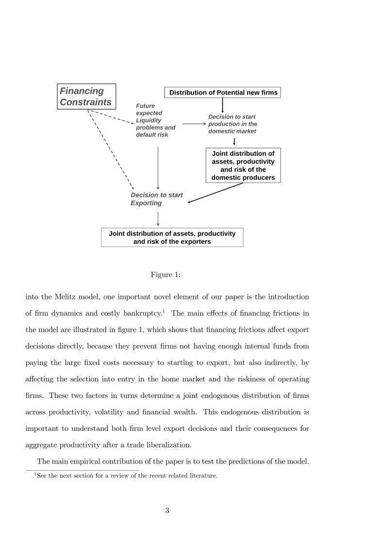
into the Melitz model, one important novel element of our paper is the introduction

of firm dynamics and costly bankruptcy.1 The main effects of financing frictions in

the model are illustrated in figure 1, which shows that financing frictions affect export

decisions directly, because they prevent firms not having enough internal funds from

paying the large fixed costs necessary to starting to export, but also indirectly, by

affecting the selection into entry in the home market and the riskiness of operating

firms. These two factors in turns determine a joint endogenous distribution of firms

across productivity, volatility and financial wealth. This endogenous distribution is

important to understand both firm level export decisions and their consequences for

aggregate productivity after a trade liberalization.

The main empirical contribution of the paper is to test the predictions of the model.

1See the next section for a review of the recent related literature.

3

To do so, we use self declared financing constraints and instrumental variables to avoid

the endogeneity problems that arise from the codetermination of productivity and

financing constraints.

In the model we consider firms that are heterogenous in their productivity and are

subject to idiosyncratic shocks. They also face financing imperfections which limit

their external financing, and therefore need to use internal funds to finance certain

investment costs which are essential for their activity. As a consequence, if their liquid

wealth is low, they may go bankrupt and be forced to liquidate their business after

a negative shock, even though it would have been profitable to continue. Financing

constraints and bankruptcy risk affect the distribution of firms in three different ways:

first, they alter the entry decision of firms inducing a positive correlation between

risk and return; second, bankruptcy affects the survival of firms, changing the pool

of producers and the nature of competition; third, financing constraints affect directly

the decision of becoming an exporter.

Firms can start exporting after paying a fixed cost. In the presence of financing

constraints this fixed cost drains some liquid wealth and increases the risk of bank-

ruptcy. In the absence of financing frictions, we obtain the standard result in Melitz

(2003): only firms with productivity above a certain threshold are willing to start ex-

porting, because the net present value of the profits from the exports is larger than the

fixed cost involved in becoming an exporter. Therefore trade liberalization increases

productivity because the most productive firms expand their activity by entering the

export market, and because the increase in competition from foreign imports will push

out of production the least productive ones.

Instead we show that in a calibrated industry affected by financing frictions (both

in the home and in the foreign country), the productivity gains induced by trade lib-

eralization are much smaller not because fewer firms export, but because the selection

4

into export is distorted by the presence of financing frictions. More specifically, financ-

ing frictions have two important effects on industry dynamics and on the outcome of

a trade liberalization.

First, the survival pattern of firms affects how their earnings evolve with time:

financing frictions imply that new and young firms have some probability to default

after a negative shock. This lowers their expected profits in the short run and deters

entry. Therefore in equilibrium fewer entrants translate into a decrease in competition,

and an increase in expected profits for the firms that survive and accumulate enough

wealth to become financially unconstrained.

In other words, the age profile of expected profits in the financially constrained

industry is more upward sloping. The default risk implies lower expected profits at

young age, that are compensated by reduced competition and higher profits for the

firms that "survive" their early age and accumulate enough wealth to be covered against

future default risk. These higher profits benefit low risk firms, which face little default

risk when young, because their income process is not very volatile. Therefore some

low risk/low productivity firms which would not start production in a perfect markets

industry, find it profitable both to start production and to start exporting after a trade

liberalization in an industry with financing frictions.

Second, the presence of financial frictions generates a risk vs. return trade off that

affects the selection of firms into entry: firms learn about the riskiness of their business

at the beginning of their life. Higher risk involves a higher likelihood of experiencing

large negative shocks that lead them to bankruptcy, and a lower chance of surviving the

initial stages of their activity. Therefore new firms that operate a very risky technology

will stay in business only if their productivity is very high. Conversely, some low pro-

ductivity/low risk firms will stay in business because their lower risk also reduces their

bankruptcy probability. This endogenous correlation amplifies the effect of financing

5

constraints, as very productive firms are also on average riskier, and therefore more

affected by financing frictions when deciding on becoming exporters. The endogenous

selection of firms into the home market implies that the most productive firms in the

industry are also on average riskier and will find it optimal to delay entering in foreign

markets until they have accumulated a sufficient amount of precautionary wealth.

We quantify these effects by calibrating an artificial industry whose dynamics match

those of our sample of Italian manufacturing firms. We show that, with respect to a

financially unconstrained industry, the presence of financing constraints and bank-

ruptcy risk reduces the productivity gains following a trade liberalization by 30% to

50%. However, the number of firms that export in the constrained and unconstrained

industry is very similar. The difference in industry productivity is entirely due to the

worsening of the selection into home production and into export induced by financing

constraints.

In the empirical section of the paper we provide evidence of these effects using a rich

dataset of Italian manufacturing firms for the period 1995-2003. This dataset contains

precise information on the trade policies of firms and on their self-declared financing

constraints. While this information on financing constraints is particularly detailed,

there is still the possibility that confounding effects such as productivity shocks that

are not fully captured by the productivity measures could be driving both exports and

financing constraints. To avoid this endogeneity problem we use standard measures of

credit availability commonly used in the relationship lending literature as instrumental

variables.

Our empirical results show that: first, the distribution of productivity in the sample

is consistent with the presence of financing constraints and entry costs in the form of

initial investments. Second, financing constraints are an important determinant of the

exporting decision of the firm, and their effect is quantitatively as important as other

6

effects identified in the literature such as size and productivity. Third, consistently

with the behavior predicted by the model, the amount of liquid assets held by the firms

around the time when they begin exporting is positively correlated with productivity

for firms that face financing frictions, while they are not correlated with productivity

for the financially unconstrained firms. Finally, we show empirically that a proxy of

the productivity of the firms becomes a worse predictor of its exporting behavior the

larger the financing constraints. For firms that are ex-ante less likely to be financially

constrained, productivity is a good predictor of their export behavior, while for firms

that are more likely to be constrained its predictive power falls.

The paper is organized as follow: Section 2 reviews the related literature; Section

3 illustrates the model; Section 4 describes the simulation results; Section 5 describes

the empirical evidence and finally Section 6 concludes.

2 Literature

The model is related to an extensive literature on firm-level export decisions started by

Melitz (2003). A sustained assumption of the models in this literature is that firms are

heterogeneous in their productivity levels and decide to become exporters by paying a

fixed initial cost. The role of financing constraints in the context of this family of mod-

els has been explored by Chaney (2005) by introducing exogenous financing constraints

as an additional source of heterogeneity across firms. In Chaney (2005) firms need cash

in advance to pay for the fixed costs of exporting and some of them are exogenously

financially constrained. Financially constrained firms never export and this, in turn,

generates reallocation effects that are different from the standard model without fi-

nancing constraints. Manova (2008) extends this framework by partially endogenizing

financing constraints. Firms are allowed to borrow a proportion of next-period’s pro-

duction. The degree of financing frictions that a firm faces is therefore modelled as the

7

proportion of next year’s production that can be borrowed this year. The risk of going

bankrupt plays an important role in our model, and a related argument can be found

in Garcia Vega and Guariglia (2007), who modify the Melitz (2003) model to introduce

idiosyncratic volatility and financing constraints. More recently, models with financing

frictions and exports have been studied by Mayneris (2010) and Berman and Hericourt

(2010).

All these models nicely embed financing constraints into the standard Melitz model.

However one important novel element of our paper is the introduction of firm dynamics.

All the above papers study "static" industries, in the sense that firms are not allowed to

retain earnings and to change their capital structure in response to financing frictions.

Conversely our paper studies a fully dynamic industry where the joint distribution

of firms across productivity, volatility and wealth arises endogenously. We show that

this endogenous distribution is very important to understand both firm level export

decisions and their consequences for aggregate dynamics after a trade liberalization.

Empirically, a number of recent papers have explored the impact of financing con-

straints on exports. Manova (2008, 2010) shows how country-sector measures of fi-

nancing constraints are negatively correlated with exports. Muuls (2008), Mayneris

(2010), Berman and Hericourt (2010) and Bellone et al. (2010) study the relation

between financing constraints and export using firm level financing constraints vari-

ables. Greenaway et al. (2007) show that seasoned exporters exhibit better financial

wealth than non exporters; while this is not true about recent exporters. This result

lends support to the idea of large fixed costs associated with entering foreign markets.

Garcia-Vega and Guariglia (2007) test their model on a sample of UK firms and show

that volatility in productivity may reduce the likelihood of becoming an exporter. All

of these papers, with the exception of Manova (2007,2008) use financing constraints

measures that are constructed using balance sheet information. The advantage of these

8

measures is that they use very standard information so they can be applied to large

samples. However these measures are correlated with productivity shocks and hard

to instrument. If productivity is measured with some error, the financing constraints

measures are likely to capture part of the effect of productivity even in a setup where

they do not matter.

Another related paper is Minetti and Chun Zhu (2010), who use a subset of the

database of Italian firms we employ in this paper to analyze the effect of financing

frictions on the intensive and extensive margins of export. Beside using a larger dataset,

our empirical analysis differs from Minetti and Chun Zhu (2010) in that we test the

specific predictions of our dynamic model regarding the direct and indirect implications

of financing frictions for the distribution of wealth and for the productivity-export

relation.2

3 The Model

We consider an industry where heterogenous firms are allowed to produce at home and

to export in a foreign market. The objective of the model is to study how financing

frictions affect the selection of firms into production, and to study the joint effect of

these frictions and of the steady state distribution of firms on the export decisions and

productivity dynamics in the industry.

We follow Melitz (2003) and Costantini and Melitz (2007) and consider a model

where each firm in an industry produces a variety of a consumption good. There is a

continuum of varieties ∈ Ω Consumers preferences for the varieties in the industry

2Other papers that do not focus on financing constraints but are nonetheless related are Campa

and Shaver (2001) and Castellani (2002). Campa and Shaver (2001) show that exporting firms may

use the exposure to different countries to diversify the risk of business cycle fluctuations. This can be

seen as a reverse causality result that shows that becoming an exporter may ease financing constraints

in the long run. Castellani (2002) studies the same database analysed in this paper, and shows that

labour productivity growth variables affect the likelihood of exports. However the levels of labour

productivity do not seem to be related to the decision to export.

9

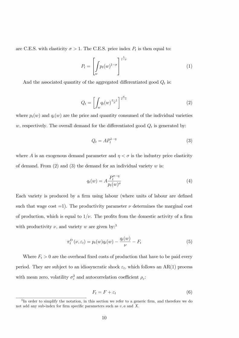
are C.E.S. with elasticity 1 The C.E.S. price index is then equal to:

=

⎡⎣Z

()1−

⎤⎦ 11−

(1)

And the associated quantity of the aggregated differentiated good is:

=

∙Z

()−1

¸ −1

(2)

where () and () are the price and quantity consumed of the individual varieties

respectively The overall demand for the differentiated good is generated by:

= 1− (3)

where is an exogenous demand parameter and is the industry price elasticity

of demand. From (2) and (3) the demand for an individual variety is:

() = −

()(4)

Each variety is produced by a firm using labour (where units of labour are defined

such that wage cost =1). The productivity parameter determines the marginal cost

of production, which is equal to 1. The profits from the domestic activity of a firm

with productivity and variety are given by:3

( ) = ()()− ()

− (5)

Where 0 are the overhead fixed costs of production that have to be paid every

period. They are subject to an idiosyncratic shock which follows an AR(1) process

with mean zero, volatility 2 and autocorrelation coefficient :

= + (6)

3In order to simplify the notation, in this section we refer to a generic firm, and therefore we do

not add any sub-index for firm specific parameters such as and

10

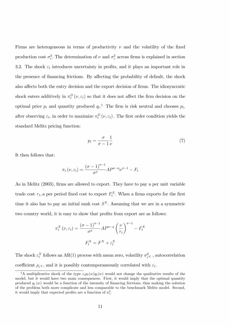
Firms are heterogeneous in terms of productivity and the volatility of the fixed

production cost 2 The determination of and 2 across firms is explained in section

3.2. The shock introduces uncertainty in profits, and it plays an important role in

the presence of financing frictions. By affecting the probability of default, the shock

also affects both the entry decision and the export decision of firms. The idiosyncratic

shock enters additively in ( ) so that it does not affect the firm decision on the

optimal price and quantity produced .4 The firm is risk neutral and chooses

after observing in order to maximize ( ) The first order condition yields the

standard Melitz pricing function:

=

− 11

(7)

It then follows that:

( ) =( − 1)−1

−−1 −

As in Melitz (2003), firms are allowed to export. They have to pay a per unit variable

trade cost a per period fixed cost to export When a firms exports for the first

time it also has to pay an initial sunk cost Assuming that we are in a symmetric

two country world, it is easy to show that profits from export are as follows:

( ) =( − 1)−1

−

µ

¶−1−

= +

The shock follows an AR(1) process with mean zero, volatility 2, autocorrelation

coefficient and it is possibly contemporaneously correlated with

4A multiplicative shock of the type ()() would not change the qualitative results of the

model, but it would have two main consequences. First, it would imply that the optimal quantity

produced () would be a function of the intensity of financing frictions, thus making the solution

of the problem both more complicate and less comparable to the benchmark Melitz model. Second,

it would imply that expected profits are a function of 2.

11

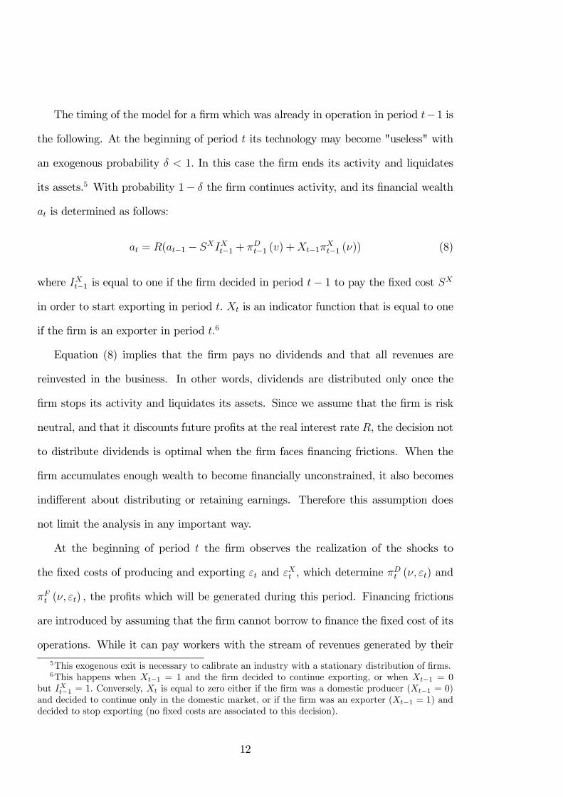
The timing of the model for a firm which was already in operation in period −1 is

the following. At the beginning of period its technology may become "useless" with

an exogenous probability 1 In this case the firm ends its activity and liquidates

its assets.5 With probability 1− the firm continues activity, and its financial wealth

is determined as follows:

= (−1 − −1 + −1 () +−1−1 ()) (8)

where −1 is equal to one if the firm decided in period − 1 to pay the fixed cost

in order to start exporting in period is an indicator function that is equal to one

if the firm is an exporter in period 6

Equation (8) implies that the firm pays no dividends and that all revenues are

reinvested in the business. In other words, dividends are distributed only once the

firm stops its activity and liquidates its assets. Since we assume that the firm is risk

neutral, and that it discounts future profits at the real interest rate , the decision not

to distribute dividends is optimal when the firm faces financing frictions. When the

firm accumulates enough wealth to become financially unconstrained, it also becomes

indifferent about distributing or retaining earnings. Therefore this assumption does

not limit the analysis in any important way.

At the beginning of period the firm observes the realization of the shocks to

the fixed costs of producing and exporting and , which determine ( ) and

( ) the profits which will be generated during this period. Financing frictions

are introduced by assuming that the firm cannot borrow to finance the fixed cost of its

operations. While it can pay workers with the stream of revenues generated by their

5This exogenous exit is necessary to calibrate an industry with a stationary distribution of firms.6This happens when −1 = 1 and the firm decided to continue exporting or when −1 = 0

but −1 = 1 Conversely, is equal to zero either if the firm was a domestic producer (−1 = 0)and decided to continue only in the domestic market, or if the firm was an exporter (−1 = 1) anddecided to stop exporting (no fixed costs are associated to this decision).

12

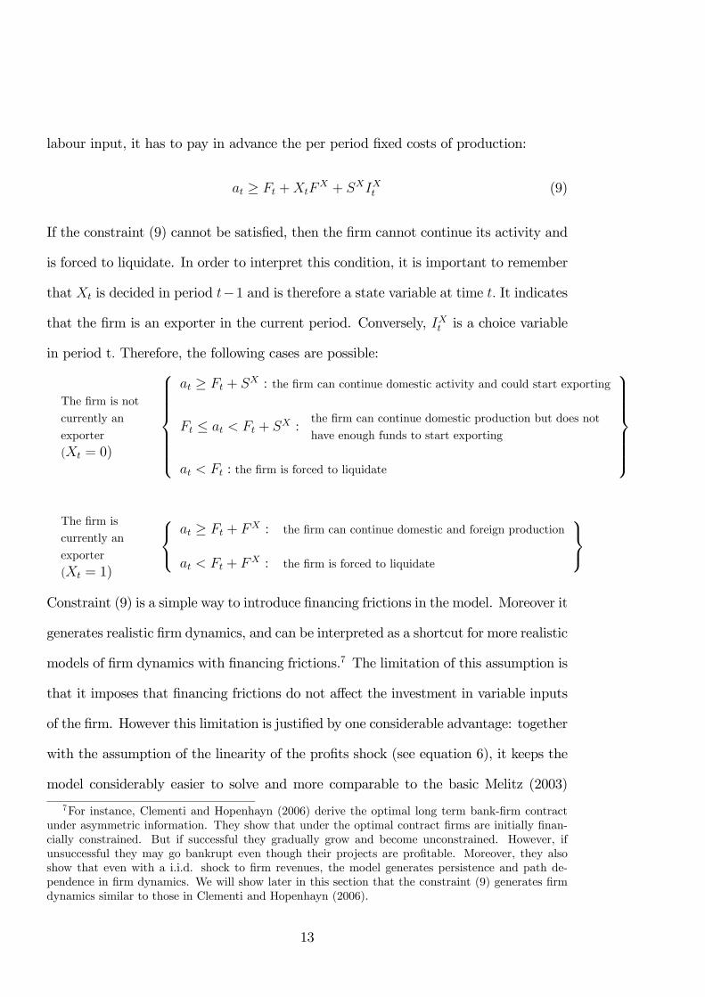
labour input, it has to pay in advance the per period fixed costs of production:

≥ + + (9)

If the constraint (9) cannot be satisfied, then the firm cannot continue its activity and

is forced to liquidate. In order to interpret this condition, it is important to remember

that is decided in period −1 and is therefore a state variable at time It indicates

that the firm is an exporter in the current period. Conversely, is a choice variable

in period t Therefore, the following cases are possible:

The firm is not

currently an

exporter

( = 0)

⎧⎪⎪⎪⎪⎪⎪⎨⎪⎪⎪⎪⎪⎪⎩

≥ + : the firm can continue domestic activity and could start exporting

≤ + :the firm can continue domestic production but does not

have enough funds to start exporting

: the firm is forced to liquidate

⎫⎪⎪⎪⎪⎪⎪⎬⎪⎪⎪⎪⎪⎪⎭The firm is

currently an

exporter

( = 1)

⎧⎨⎩ ≥ + : the firm can continue domestic and foreign production

+ : the firm is forced to liquidate

⎫⎬⎭Constraint (9) is a simple way to introduce financing frictions in the model. Moreover it

generates realistic firm dynamics, and can be interpreted as a shortcut for more realistic

models of firm dynamics with financing frictions.7 The limitation of this assumption is

that it imposes that financing frictions do not affect the investment in variable inputs

of the firm. However this limitation is justified by one considerable advantage: together

with the assumption of the linearity of the profits shock (see equation 6), it keeps the

model considerably easier to solve and more comparable to the basic Melitz (2003)

7For instance, Clementi and Hopenhayn (2006) derive the optimal long term bank-firm contract

under asymmetric information. They show that under the optimal contract firms are initially finan-

cially constrained. But if successful they gradually grow and become unconstrained. However, if

unsuccessful they may go bankrupt even though their projects are profitable. Moreover, they also

show that even with a i.i.d. shock to firm revenues, the model generates persistence and path de-

pendence in firm dynamics. We will show later in this section that the constraint (9) generates firm

dynamics similar to those in Clementi and Hopenhayn (2006).

13

model. Moreover, to use a more realistic financing frictions assumption is not likely to

change the main results of the model. This is because, as it will be explained later,

the liquidation risk implies that firms accumulate a precautionary stock of liquid assets

before starting to export. Therefore, if we assumed that also variable production inputs

were subject to financing frictions, the production decisions of exporting firms would

not be likely to change because these precautionary assets would be large enough to

allow the self financing of all variable inputs.

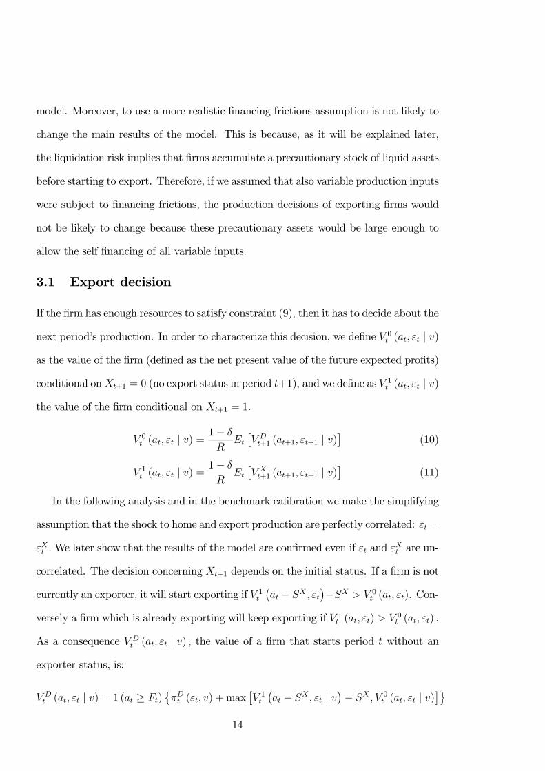
3.1 Export decision

If the firm has enough resources to satisfy constraint (9), then it has to decide about the

next period’s production. In order to characterize this decision, we define 0 ( | )

as the value of the firm (defined as the net present value of the future expected profits)

conditional on+1 = 0 (no export status in period +1), and we define as 1 ( | )

the value of the firm conditional on +1 = 1.

0 ( | ) =

1−

£ +1 (+1 +1 | )

¤(10)

1 ( | ) =

1−

£ +1 (+1 +1 | )

¤(11)

In the following analysis and in the benchmark calibration we make the simplifying

assumption that the shock to home and export production are perfectly correlated: =

We later show that the results of the model are confirmed even if and are un-

correlated. The decision concerning +1 depends on the initial status. If a firm is not

currently an exporter it will start exporting if 1

¡ −

¢− 0 ( ). Con-

versely a firm which is already exporting will keep exporting if 1 ( ) 0

( )

As a consequence ( | ) the value of a firm that starts period without an

exporter status, is:

( | ) = 1 ( ≥ )

© ( ) + max

£ 1

¡ − |

¢− 0 ( | )

¤ª14

and the value of a firm which start period with an exporter status is

( | ) = 1

¡ ≥ +

¢ © ( ) + ( ) + max

£ 1 ( | ) 0

( | )¤ª

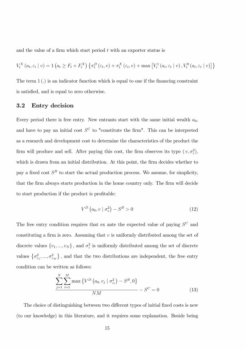
The term 1 () is an indicator function which is equal to one if the financing constraint

is satisfied, and is equal to zero otherwise.

3.2 Entry decision

Every period there is free entry. New entrants start with the same initial wealth 0

and have to pay an initial cost to "constitute the firm". This can be interpreted

as a research and development cost to determine the characteristics of the product the

firm will produce and sell. After paying this cost, the firm observes its type ( 2)

which is drawn from an initial distribution. At this point, the firm decides whether to

pay a fixed cost to start the actual production process. We assume, for simplicity,

that the firm always starts production in the home country only. The firm will decide

to start production if the product is profitable:

¡0 | 2

¢− 0 (12)

The free entry condition requires that ex ante the expected value of paying and

constituting a firm is zero. Assuming that is uniformly distributed among the set of

discrete values 1 and 2 is uniformly distributed among the set of discrete

values©21

2

ª and that the two distributions are independent, the free entry

condition can be written as follows:

X=1

X=1

max©

¡0 | 2

¢− 0ª

− = 0 (13)

The choice of distinguishing between two different types of initial fixed costs is new

(to our knowledge) in this literature, and it requires some explanation. Beside being

15

realistic to distinguish between the startup costs to define the product and the costs

to actually start producing it, this definition allows to analyze the selection role of

financing imperfections. The pre-entry cost is the one that determines the amount

of potential entrants, while determines the characteristics of entrants. We show

that given a draw of and 2 the value of entering the market (0 | 2) decreases

in 2 in the presence of financing frictions, because the higher is 2 the more volatile

are profits, and the higher is the risk that the firm will hit a binding constraint (9)

and be liquidated. Since (0 | 2) also increases in it follows that financing

frictions generate an endogenous positive correlation between idiosyncratic risk and

productivity. This positive correlation, of which we find strong evidence in the data,

has important consequences for the effect of financing frictions on export dynamics, as

it will be shown below.

3.3 Industry equilibrium

We consider a steady state industry equilibrium where the aggregate price the

aggregate quantity and the distribution of firms over the values of and 2

are constant over time. The presence of the exogenous exit probability ensures

that the distribution of wealth across firms is non-degenerate. Aggregate price is

set to ensure that the free entry condition (13) is satisfied. The number of firms in

equilibrium ensures that also satisfies the aggregate price equation (1). Aggregation

is very simple because, as in Melitz (2003), all operating firms with productivity

choose the same price () as determined by (7).

4 Model’s solution and calibration

The solution of the model is obtained using a numerical method (see Appendix I for

a description). The time period is one year, and the benchmark parameters are as

16

follows: the aggregate productivity termmatches the number of firms in the empirical

dataset analyzed in the next section. The exit probability is set to 0.04, matching the

average exit rate of firms observed in the empirical data. The real interest rate is set

equal to 2%. Following Constantini and Melitz (2007) the fixed costs is calibrated

so that firms on average devote 20% of their labour cost to overhead. is set equal

to

The technological parameters 2 and match the firm dynamics estimated us-

ing our dataset of Italian manufacturing firms. The uniform distribution of ∈ [ ]

matches the cross sectional distribution of the profits/sales ratio. The distribution

of the volatility of the shock 2 is uniform between 0 and 2 where 2 is chosen to

match the average coefficient of variation of the profits/sales ratio at the firm level.

The autocorrelation coefficient matches the autocorrelation of the profits/sales ra-

tio. The fixed export cost corresponds to a sunk cost of starting to export equal

to 25% of average yearly sales in the industry. This is in line with Das, Roberts, and

Tybout (2007), who estimate for Colombian chemical plants that export penetration

costs account for between 18.4 and 41.2 percent of the annual value of a firm’s ex-

ports. The startup cost matches the average profitability of firms; the fixed cost

of starting production affects the selection into entry and the relation between risk

and volatility of new firms. Therefore it is chosen in order to match the difference in

the correlation between volatility and profits between constrained and unconstrained

firms.8

The variable trade cost matches the fraction of exporting firms for which exports

account for at least 20% of total sales.9 The value of initial wealth 0 determines the

8For both the empirical and the simulated correlations we consider time series of 9 observations

for each firm.9The threshold of 20% does not affect the simulated statistics, because all simulated firms that

start exporting do indeed export a large fraction of their total production. It is instead important

for the empirical data, where some firms may export small quantities simply because they are using

17

intensity of financing frictions and the probability of bankruptcy for young firms. It is

calibrated in order to match the fraction of financially constrained firms.10 Among the

parameters that we do not directly calibrate, the elasticities and are taken from

Melitz and Costantini (2007), and is assumed to be perfectly correlated to 11

-table 1 about here-

Table 1 summarizes the calibrated parameters and the matched moments. The

parameter values match the chosen moments reasonably well. In particular, the sim-

ulated firms are very similar to those in the dataset concerning the level, volatility

and cross sectional dispersion of profits. Moreover in the simulated dataset on aver-

age 0.36% of firms default every period because of a binding liquidity constraint (9).

This is of a similar order of magnitude of the frequency of yearly defaults observed for

manufacturing firms (around 0.5%-1%). The simulated data are also consistent with

the stylized fact that the exit rate of firms is age dependent. The exit rate of firms in

the first year of age is 9%, in the second year is 5.5%, in the third year is 4.8% and

then it gradually converges to the constant exogenous exit rate of 4%. The simulated

data also matches well the fraction of exporting Italian firms. More than 50% of the

firms in the sample export a substantial amount of their products in our sample. On

the one hand, this empirical fact depends on two features of the Italian industry: i)

the presence of a large number of small firms specialised in producing and exporting

high quality manufactured goods; ii) the high level of trade integration of North Italy

(where are located around 90% of all the Italian manufacturing firms) with Continental

indirect channels and they did not invest the sunk cost to establish a proper presence in the foreign

markets.10In the empirical dataset we detect on average 14% of firms that every period complain about the

lack of external finance availability. In the simulated data, for the firms that continue activity, the

only financially constrained investment is the export decision. Firms cannot borrow, and therefore in

order to be able to continue activity in period and to start exporting in period + 1 , their wealth

need to cover both the fixed cost and the sunk cost

11This perfect correlation assumption simplifies the numerical solution of the model, but it is not

essential for the results.

18

Europe. On the other hand, the main results of the model still hold for alternative

calibrations with a much smaller fraction of exporting firms, as it will be shown later

in table 4.

4.1 Simulations results

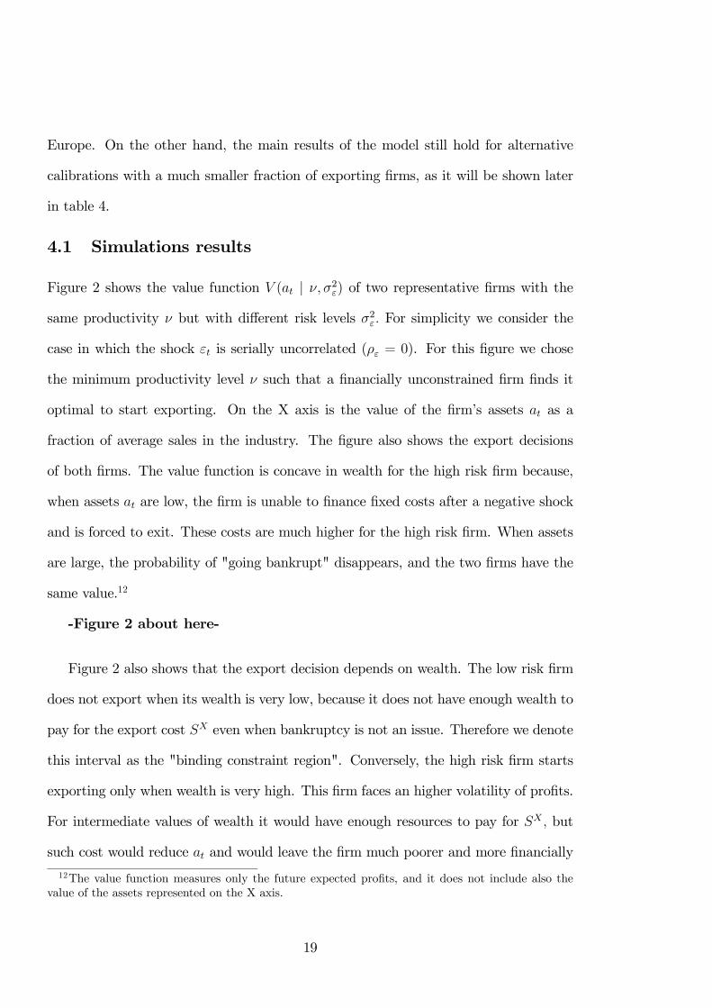
Figure 2 shows the value function ( | 2) of two representative firms with the

same productivity but with different risk levels 2 For simplicity we consider the

case in which the shock is serially uncorrelated ( = 0). For this figure we chose

the minimum productivity level such that a financially unconstrained firm finds it

optimal to start exporting. On the X axis is the value of the firm’s assets as a

fraction of average sales in the industry. The figure also shows the export decisions

of both firms. The value function is concave in wealth for the high risk firm because,

when assets are low, the firm is unable to finance fixed costs after a negative shock

and is forced to exit. These costs are much higher for the high risk firm. When assets

are large, the probability of "going bankrupt" disappears, and the two firms have the

same value.12

-Figure 2 about here-

Figure 2 also shows that the export decision depends on wealth. The low risk firm

does not export when its wealth is very low, because it does not have enough wealth to

pay for the export cost even when bankruptcy is not an issue. Therefore we denote

this interval as the "binding constraint region". Conversely, the high risk firm starts

exporting only when wealth is very high. This firm faces an higher volatility of profits.

For intermediate values of wealth it would have enough resources to pay for but

such cost would reduce and would leave the firm much poorer and more financially

12The value function measures only the future expected profits, and it does not include also the

value of the assets represented on the X axis.

19

fragile. Thus this high risk firm prefers to wait and to accumulate more assets, for

precautionary reasons, before starting to export. Therefore the wealth interval in which

only the low risk firm exports identifies the "precautionary region". In this particular

case the value function is virtually flat for assets values in the precautionary region

because the chosen value of implies that the net present value of starting to export

is very small for these firms.

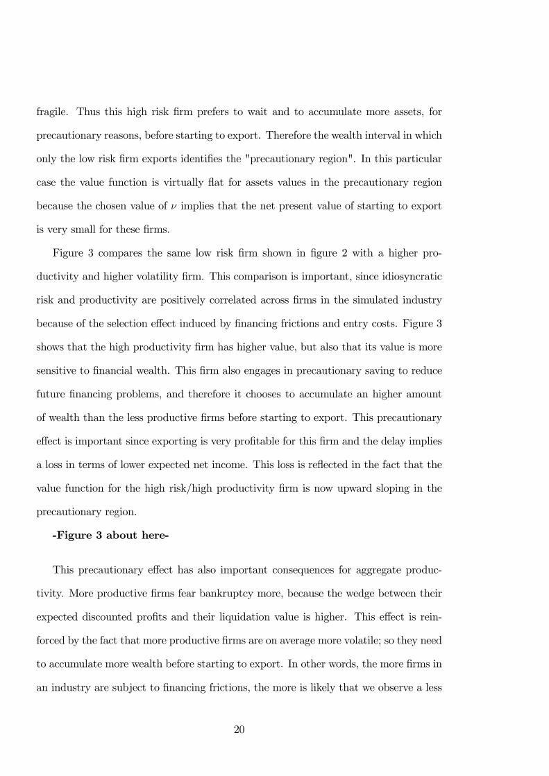
Figure 3 compares the same low risk firm shown in figure 2 with a higher pro-

ductivity and higher volatility firm. This comparison is important, since idiosyncratic

risk and productivity are positively correlated across firms in the simulated industry

because of the selection effect induced by financing frictions and entry costs. Figure 3

shows that the high productivity firm has higher value, but also that its value is more

sensitive to financial wealth. This firm also engages in precautionary saving to reduce

future financing problems, and therefore it chooses to accumulate an higher amount

of wealth than the less productive firms before starting to export. This precautionary

effect is important since exporting is very profitable for this firm and the delay implies

a loss in terms of lower expected net income. This loss is reflected in the fact that the

value function for the high risk/high productivity firm is now upward sloping in the

precautionary region.

-Figure 3 about here-

This precautionary effect has also important consequences for aggregate produc-

tivity. More productive firms fear bankruptcy more, because the wedge between their

expected discounted profits and their liquidation value is higher. This effect is rein-

forced by the fact that more productive firms are on average more volatile; so they need

to accumulate more wealth before starting to export. In other words, the more firms in

an industry are subject to financing frictions, the more is likely that we observe a less

20

productive firm which chooses to start exporting while a more productive one chooses

to wait. At the aggregate level, this reduces the beneficial effect of trade liberalization

on the reallocation of production.

In order to quantify the aggregate effect of financing frictions on firm dynamics after

trade liberalization we simulate several calibrated artificial industries for many periods,

and we compute their steady state statistics. We consider three different industries: one

with perfect financial markets, and no financing frictions; one with financing frictions

but no default risk, and one with both financing frictions and default risk. These three

industries are identical in terms of all the parameters illustrated before, except the

following: in the "Financing frictions only" industry the profits shock is equal to zero,

= 0 for any This industry is similar to those analyzed by Manova (2008) and

Chaney (2005). Profits are not volatile, but some firms do not export because they

have insufficient internal funds to finance the export cost . In the "perfect markets"

industry instead initial wealth 0 is high enough so that no firm is ever financially

constrained in its investment decisions, regardless of its volatility 2. Therefore firm

dynamics in this industry are the same as in the standard Melitz model.

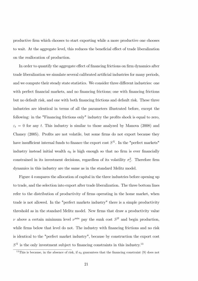
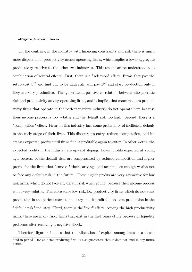
Figure 4 compares the allocation of capital in the three industries before opening up

to trade, and the selection into export after trade liberalization. The three bottom lines

refer to the distribution of productivity of firms operating in the home market, when

trade is not allowed. In the "perfect markets industry" there is a simple productivity

threshold as in the standard Melitz model. New firms that draw a productivity value

above a certain minimum level min pay the sunk cost and begin production,

while firms below that level do not. The industry with financing frictions and no risk

is identical to the "perfect market industry", because by construction the export cost

is the only investment subject to financing constraints in this industry.13

13This is because, in the absence of risk, if 0 guarantees that the financing constraint (9) does not

21

-Figure 4 about here-

On the contrary, in the industry with financing constraints and risk there is much

more dispersion of productivity across operating firms, which implies a lower aggregate

productivity relative to the other two industries. This result can be understood as a

combination of several effects. First, there is a "selection" effect. Firms that pay the

setup cost and find out to be high risk, will pay and start production only if

they are very productive. This generates a positive correlation between idiosyncratic

risk and productivity among operating firms, and it implies that some medium produc-

tivity firms that operate in the perfect markets industry do not operate here because

their income process is too volatile and the default risk too high. Second, there is a

"competition" effect. Firms in this industry face some probability of inefficient default

in the early stage of their lives. This discourages entry, reduces competition, and in-

creases expected profits until firms find it profitable again to enter. In other words, the

expected profits in the industry are upward sloping. Lower profits expected at young

age, because of the default risk, are compensated by reduced competition and higher

profits for the firms that "survive" their early age and accumulate enough wealth not

to face any default risk in the future. These higher profits are very attractive for low

risk firms, which do not face any default risk when young, because their income process

is not very volatile. Therefore some low risk/low productivity firms which do not start

production in the perfect markets industry find it profitable to start production in the

"default risk" industry. Third, there is the "exit" effect. Among the high productivity

firms, there are many risky firms that exit in the first years of life because of liquidity

problems after receiving a negative shock.

Therefore figure 4 implies that the allocation of capital among firms in a closed

bind in period 1 for an home producing firm, it also guarantees that it does not bind in any future

period.

22

economy is worsened by financing frictions and default risk. The remaining three "cir-

cled" lines in figure 4 represent the distribution of exporting firms when the industry

opens up to trade.14 By construction the vertical distance between the "active firms"

line and the "exporters" line measures the positive reallocation effect induced by the

selection into export. The larger the distance, the more export activity is concentrated

among the more productive firms, and the more liberalizing trade promotes a reallo-

cation of production towards the more productive firms.15 Figure 4 shows that such

distance is much smaller in the financially constrained industry, showing that financing

frictions worsen the selection into export. In other words, in the presence of default

risk productivity becomes less important in determining the decision to export, and

therefore trade liberalization has a smaller impact on the reallocation of capital than

in the "perfect markets" industry.

This result is also best explained by distinguishing several effects: first, there is a

direct effect. Only firms that accumulate enough wealth to pay the sunk cost may

start exporting. This effect actually increases the importance of productivity for the

export decision, because more productive firms accumulate wealth faster on average.

However, the selection effect and the competition effect mentioned before worsen the

selection into export. According to the selection effect, more productive firms are on

average more risky, and need to accumulate more financial wealth before starting to

export. According to the competition effect, some low risk/low productivity firms,

which would only operate in the home market in the absence of financing frictions,

find it profitable to export in the industry with default risk, due to the higher profits

14Each industry opens up to trade in a symmetric two country world, where the foreign country

industry shares the same characteristics.15The total effect of trade liberalization on productivity is given by this reallocation effect, weighted

by the number of exporting firms, and by the competition effect that pushes out of production some

firms that were previously operating in the home market. This latter effect is not shown in figure 4,

but is analysed more in details in tables 2-4.

23

enjoyed by the firms that do not default. Figure 4 also shows that the selection into

export in the industry with "financing frictions only", where there is no default risk,

no selection effect, and a very small competition effect, is very similar to the selection

in the perfect markets industry.

-Figure 5 about here-

Figure 4 jointly analyze the impact of the selection and competition effects on

export decision, while figures 5 and 6 focus on the former one. Figure 5 shows the

accumulation of financial assets for firms grouped according to the parameter 2 (the

volatility of profits). In the industry "with financing frictions only" firms do not go

bankrupt, and they accumulate exactly the amount of assets necessary to finance the

sunk cost to start exporting. The volatility of profits has no effect on the export

decision in this industry. Conversely in the industry with default risk the higher is the

volatility of profits, the higher are average profits, because of the selection effect, but

also the higher are the assets accumulated before starting to export. The difference in

the accumulation of assets between the two industries is entirely due to precautionary

saving. Figure 6 shows that such precautionary behavior significantly increases the

time necessary to start exporting for the most volatile firms. Firms that discover to

be high risk enter into production only if they are very productive, and then they wait

much longer before starting to export than the less productive and volatile firms.

-Figure 6 about here-

The implications of figures 4-6 is that the gain in aggregate productivity from

liberalizing trade may be significantly smaller in the presence of financing frictions not

because fewer firms export, but because selection into export is not efficient. This

prediction of the model is quantified in table 2. In the first three columns we compare

the same three industries analyzed in figure 4. The first row shows the percentage of

24

exporting firms. In the "financing frictions only" economy 36.6% of firms export, versus

a value of 49.9% in the "perfect markets" economy. This difference is due to the firms

that cannot pay for the sunk cost when their wealth is too low. Conversely the

percentage of exporting firms is much higher in the "default risk" economy, being equal

to 48%. Here the direct negative effect is also operational, but it is counterbalanced

by the general equilibrium effect mentioned before, which has a positive effect on the

probability to export. The second row of table 2 shows the gain in productivity caused

by trade liberalization. The percentage value is measured relative to the productivity

in the "default risk" industry before opening up to trade. Moreover it is standardized

so that a 100% value would imply that after trade liberalization all production is

carried out by the firms with the highest productivity in the distribution The figure

shows that the gain in productivity is more than 30% smaller in the "Default risk"

industry with respect to the "Perfect markets" industry. This reduction is not caused

by a reduction in the number of exporting firms, which is approximately equal in the

two industries. Instead it is due to a worsening in the selection of firms into home

production, and to a worsening of the selection of firms into export. On the contrary

the reduction in productivity gains is much smaller in the "financing frictions only"

industry, despite fewer firms export here, because selection into export is as good as

in the perfect markets economy.

-Table 2 about here-

These results imply that financing frictions may significantly affect firm dynamics

after a trade liberalization not simply because firms are unable to export, as it has been

suggested by the previous literature, but because they worsen the selection both into

home and into foreign markets. We show that this selection effect is quantitatively

important in affecting the productivity gains from trade liberalization. One possi-

25

ble objection of this result is that access to foreign markets may actually reduce the

volatility of profit by diversifying the revenues shocks (see Campa and Shaver 2001).

We consider this possibility in the fourth column of table 2, which assumes that rev-

enues from export are not subject to uncertainty ( = 0 always). Therefore exporting

reduces the volatility of profits in relative terms, and this reduction is larger the riskier

a firm is. This is of course an extreme example, because in reality it is plausible to

assume that and have a certain degree of positive correlation. Nonetheless table

2 shows that, even when export is not risky, the default risk substantially reduces the

increase in average productivity caused by trade liberalization. This is because the

competition effect described before is still present, since it is determined by the risk

of entering in the home production. Moreover the selection effect becomes less strong,

but it does not disappear completely.

4.2 Sensitivity analysis

Tables 3 and 4 analyze the robustness of the results illustrated in the previous sections

for different calibrations.

-Table 3 about here-

Table 3 shows industry dynamics in the "default risk" industry with alternative

calibrations of the volatility parameter 2 the initial wealth 0 and the persistency pa-

rameter These three parameters affect the wealth distribution, and change industry

dynamics only in the industry with financing frictions, because wealth is irrelevant for

the production decisions of firms in the perfect markets industry. Among the results

shown in table 3, it is worth noting that the general result of a smaller increase in

productivity holds across all the specifications. However, when financing frictions are

less strong because volatility of profits is smaller (2 = 05) or because initial wealth is

larger (0 = 032) then the worse reallocation of capital is almost entirely due to the

26

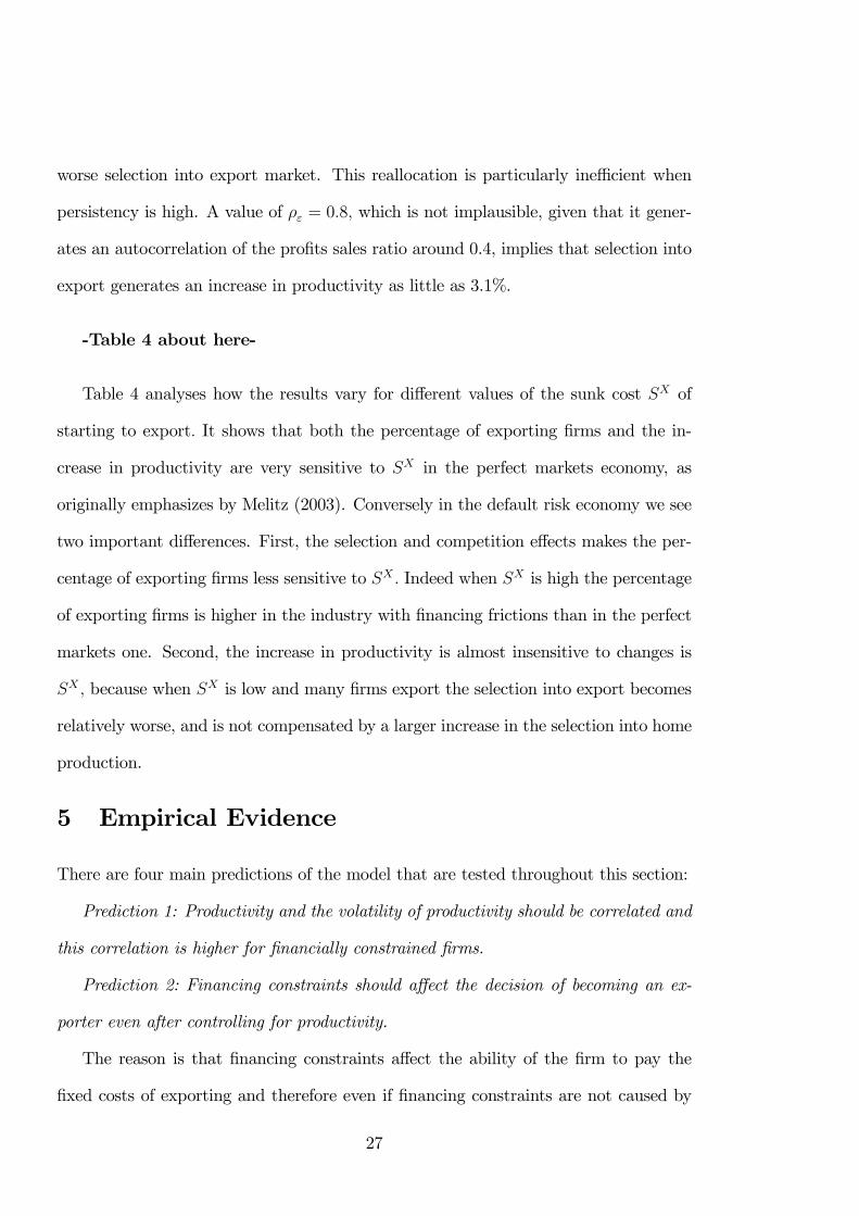
worse selection into export market. This reallocation is particularly inefficient when

persistency is high. A value of = 08 which is not implausible, given that it gener-

ates an autocorrelation of the profits sales ratio around 0.4, implies that selection into

export generates an increase in productivity as little as 3.1%.

-Table 4 about here-

Table 4 analyses how the results vary for different values of the sunk cost of

starting to export It shows that both the percentage of exporting firms and the in-

crease in productivity are very sensitive to in the perfect markets economy, as

originally emphasizes by Melitz (2003). Conversely in the default risk economy we see

two important differences. First, the selection and competition effects makes the per-

centage of exporting firms less sensitive to Indeed when is high the percentage

of exporting firms is higher in the industry with financing frictions than in the perfect

markets one. Second, the increase in productivity is almost insensitive to changes is

because when is low and many firms export the selection into export becomes

relatively worse, and is not compensated by a larger increase in the selection into home

production.

5 Empirical Evidence

There are four main predictions of the model that are tested throughout this section:

Prediction 1: Productivity and the volatility of productivity should be correlated and

this correlation is higher for financially constrained firms.

Prediction 2: Financing constraints should affect the decision of becoming an ex-

porter even after controlling for productivity.

The reason is that financing constraints affect the ability of the firm to pay the

fixed costs of exporting and therefore even if financing constraints are not caused by

27

productivity they should still matter in determining the firm’s exporting behavior.

Prediction 3: Financially constrained firms should hoard liquidity around the mo-

ment when they become exporters, for precautionary reasons.

While financially unconstrained firms can borrow to pay for the large initial fixed

costs of exporting, financially constrained firms will accumulate enough liquid assets

so that even after paying for the initial export costs they will have enough resources

to face future demand shocks in both the home and the export market. Furthermore,

productivity affects this precautionary liquidity hoarding in two ways: it tends to reduce

it because more productive firms expect on average to accumulate wealth faster once

they start exporting. But also it tends to increase it because productive firms are also

riskier, and hence need more liquidity to absorb bigger shocks. If the second effect

prevails (as it does in the calibrated simulated industries analyzed in the previous

section), then the liquidity hoarding should be stronger for more productive firms.

Prediction 4: The effect of the firm’s individual productivity on the likelihood of

being an exporter should be smaller the higher the financing constraints.

While in an unconstrained industry a strict threshold of productivity should deter-

mine whether a firm exports or not, this threshold gets blurred the moment financing

constraints appear. On the one hand some high risk/high productivity firms prefer to

delay the export decision, on the other hand some low productivity/low risk firms are

more likely to continue operating in both the home and foreign market. The intuition

for this result is captured in figures 3 and 4.

5.1 Data Description

To test the empirical predictions of the model we use the dataset of the Mediocredito

Centrale surveys. The dataset contains a representative sample of Small and Medium

Italian manufacturing firms. It is an incomplete panel with two main sources of infor-

28

mation gathered in two different surveys:

i) Balance sheet data and profit and loss statements from 1995 to 2003 at a year

level (index ).

ii) Qualitative information from three surveys conducted in 1997, 2000, 2003. Each

survey (indexed ) reports information about the activity of the firm in the three pre-

vious years and in particular, it includes detailed information on exports and financing

constraints.

Each survey is conducted on a representative sample of the population of small and

medium manufacturing firms (smaller than 500 employees). The samples are selected

balancing the criterion of representativeness with the one of continuity. The firms in

each survey contain three consecutive years of data. After the third year 2/3 of the

sample is replaced and the new sample is then kept for the three following years.

This dataset is particularly well suited for our analysis. It contains firm-level de-

tailed information about financing constraints, information about the exporting be-

havior of the firm and standard accounting data. Once we restrict ourselves to the

observations with valid information the relevant variables the dataset contains 6966

firms and 31939 firm-year observations.

The firm-level variables about international trade that we use in the analysis are: A

dummy variable that measures whether the firm exports part of its production (export

dummy), the % of sales exported (% sales exported ) and the number of regions to

which the firm exports out of a maximum of 8 different international regions (number

of regions).16 17

16The regions are EU, Africa, Asia, China, USA-Canada, Central and South America, Oceania,

Other.17In most of the regressions throughout the paper there is not enough within firm variation to justify

the use of fixed effects regressions. The reasons for this are that 2/3 of the sample is replaced in each

3 year wave, that some variables do not change buy construction throughout the 3 years window and

that there is substantial persistence in both trade and financing constraints variables.

29

As our main measure of financing constraints we consider the questions in the

Survey where each firm is asked:

i) Whether it had a loan application turned down recently.

ii) Whether it desires more credit at the market interest rate.

iii) Whether it would be willing to pay an higher interest rate than the market rate

in order to obtain credit.

We use this information to construct our main measure of financing constraints

constrained which takes value 1 for period if firm answers yes to any of the

questions (i) to (iii) and takes value zero otherwise. According to this measure 14% of

the firms declare to be financially constrained. This is a much more reliable measure

of financing constraints than measures based on balance sheet information or financial

outcomes. However a possible concern is that this variable could be correlated with

productivity shocks which are likely determinants of trade outcomes. For this reason

we use an instrumental variables approach using as IVs variables that are unlikely to

be correlated with productivity shocks.

In all the regressions we introduce as controls the size of the firm measured as

the log of its real total assets (Log real total assets), the age of the firm in years

(Age (years)) and age squared (Age squared ) and the productivity level of the firm

(TFP ). Productivity is measured as the residual from a regression model in which

total production is explained by a translog specification of a Cobb Douglas production

model that includes fixed capital and total employment. The coefficients of the model

are allowed to vary at a 2 digit-sector level and on 3 year windows.18 This measure

of productivity is quite standard in the empirical literature. Furthermore, Crino and

Epifani (2010) use the Mediocredito dataset to study how firm and foreign market

18In particular productivity is measured by in the following model () =P=1

P=1 log() + log() + log() ∗ log() + + +

w where referes to 2 digit sector levels, to 3 year intervals and to the years 1995 to 2003.

30

characteristics affect the geographic distribution of exporters’ sales. They calculate

several measures of total factor productivity and show that the results based on a

Cobb-Douglas translog specification are similar to the results based on alternative

measures of productivity, such as a Cobb-Douglas specification with the semiparametric

estimators proposed by Olley and Pakes (OP, 1996) and Levinsohn and Petrin (2003).

Furthermore, it is important to note that our theoretical model is very stylized, and

not entirely consistent with using a standard TFP measure as a proxy of productivity.

We pick this particular measure for consistency and comparability with the existing

literature. The results are however robust to using a productivity measure based on

gross profits (sales minus variable costs) which is entirely consistent with the model.

5.2 Identification strategy

Both exports and financing constraints are likely to be correlated with the levels of

productivity of the firm. Given that our productivity measure is an imperfect proxy

for true productivity it would be possible that the measure of financing constraints

would be partially capturing the effect of productivity. That is, if productivity is

correlated with exports and our productivity proxy measures it with error, the financing

constraints measure may also be proxying for productivity. For this reason we need

to instrument our financing constraints measure with instrumental variables that are

uncorrelated with productivity shocks and unlikely to affect exports through channels

other than financing constraints.

We use a set of instrumental variables similar to the ones used in Caggese and

Cuñat (2008). A first approach uses as instrumental variable that measures the level

of financial development at a regional level (Financ. Dev ). This variable is calculated

in Guiso, Sapienza and Zingales (2004) and it measures the likelihood that a consumer

bank loan is denied in different Italian regions. The measured is “inverted” and nor-

31

malized, so that a value of zero indicates the highest probability of denial and that the

maximum possible value is 0.56. While this variable is uncorrelated with temporary

liquidity shocks that the firm may have, it is possible that, cross sectionally, it is cor-

related with variables that jointly determine financing constraints and the propensity

to export. For this reason we use a second set of instruments that are based on the

relationship lending literature. These variables are the share the main lending bank

has over the total loans of the firm (Percentage loans with main bank ), the number

of years that the firm has been operating with this bank (length of main bank relation-

ship) and the square of this same variable (length of main bank relationship squared ).

This set of instruments is referred to as Rel lending IV in the regressions.

Table 5 justifies the validity of these variables as instruments of financing constraints

and shows the first stage of the IV regressions.

-table 5 about here-

In column 1 we pool all four variables and add some balance sheet variables that are

correlated with financing constraints. These are the leverage ratio of the firm (Leverage

ratio), its net financial assets over total assets (Liquidity ratio) and the coverage ratio

(Coverage ratio). This is a form of validation of our measure of financial constraints

that is correlated with balance sheet measures of constraints. With respect to the

instrumental variables, the table shows that higher financial development reduces the

likelihood of being financially constrained. A larger share of loans with the main bank

is however related to higher financing constraints. This has been identified in the

relationship lending literature as a consequence of higher monopoly power of the bank.

Longer relationship with the main bank reduces the likelihood of being financially

constrained in a convex way. Columns 2 and 3 show the first stage regressions of the

two sets of instrumental variables.

32

5.3 Results

In Table 6 we verify the first prediction of the model, showing the relationship be-

tween firm productivity and its volatility. The measure of firm productivity is the TFP

variable described in section 5.1. The measure of volatility in columns 1 to 3 is the

firm-level standard deviation of this same measure and we interact it with dummies

that correspond to the firms in the top and middle third of predicted financing con-

straints according to the first stage regression in Table 6 column 3 (i.e. using the

instruments share main bank yearsbank years2). More specifically, we first pre-

dict the variable everconstrained using our instrumental variables. The variable is

averaged at a firm level and used to generate three dummy variables ,

, and that split the sample in roughly three equal

parts (with being the omitted variable in the regressions) according

to the predicted financing constraints of the firm. The variables are then interacted with

the volatility of the productivity of the firm. The correlation between the predicted

financing constraints and the productivity measure is 0.009. This is not surprising,

given the way that they are constructed but it is important to emphasize it, as the

interacted variables should represent comparable populations of firms in terms of pro-

ductivity but with different levels of financing constraints. Column 3 includes controls

for log assets, age, age squared, year, sector and regional dummies.

-table6 about here-

The results in columns 1 to 3 show that indeed, productivity is correlated with its

volatility and that this correlation is higher for those firms that are more constrained.

In columns 4 to 6 we replicate the analysis but using the standard deviation of pro-

ductivity divided by log net sales to measure volatility. This alternative measure is

a unit independent measure of volatility and therefore less sensitive to the influence

33

of the size of firms in determining volatility.19 This is a much more strict test of the

correlation between productivity and its volatility and, in fact, the model does not

predict that this ratio is necessarily growing on productivity; this is only the case when

selection into entry is quite strong. The results are however quite similar to the ones in

columns 1 and 2 showing that the volatility of productivity is positively correlated with

productivity but that the effect is mainly coming from financially constrained firms.

Table 7 verifies the second prediction of the model, showing the basic results of the

influence of financing constraints on the exporting policies of firms. The main control

variables replicate some of the results already present in the literature. Larger sizes and

higher productivity levels are associated with a higher likelihood of exporting, higher

proportion of exports and more destination regions. Age is also positively correlated

with the likelihood of being an exporter in general and in particular markets; however

age does not seem to have much impact on the intensive margin of exports.

-table 7 about here-

The main results of this table are the ones on the financing constraints variable.

Constrained firms are less likely to export when financing constraints are instrumented

(columns 2 and 3). This is an important result. Even after controlling for productivity,

size, age, sector and year effects, financing constraints still retain power in explaining

exports. This effect is unlikely to be the result of financing constraints capturing a

productivity residual, given the nature of our instrumental variables.20 Interestingly,

financing constraints do not seem to affect the percentage of sales exported (columns

19Note that an alternative unit-independent measure is the coefficient of variation of TFP (i.e.

sdTFP/meanTFP), but given that the average TFP is by construction zero at a sector-period level,

the coefficient of variation leads to frequent outliers in this case.20The results are consistent with Manova (2008) and Muûls and Pisu (2009) that show that measures

of financing constraints based on balance sheed and sector data are negatively correlated with exports.

However a general theme in both papers is that financing constraints are largely determined by

productivity. From an identification point of view, it is difficult to disentangle what part of their

results is due to direct or indirect effects of productivity. Our instrumental variables approach is

unlikely to be capturing productivity effects on the constraints measure.

34

4 to 6). This is consistent with the idea that financing constraints are relevant for the

fixed costs of exporting, but less relevant on the intensive margin, where the exported

goods can serve as collateral and international trade credit is generally available.21

Importantly, it is also consistent with the prediction of the model that firms start to

export only after they accumulated some financial assets for precautionary reasons,

in order to reduce future financing problems. Finally (in columns 7 to 9), financing

constraints also affect negatively the number of international regions to which the firm

exports. This last effect seems quite strong and may be related to the existence of

fixed exporting costs that are region-specific (e.g. having a firm representative in each

region or adapting goods to regional tastes).

The next set of results verify the third prediction of the model by showing the

evolution of liquidity when firms become exporters. In table 8 the dependent variable

is a measure of liquidity constructed as total cash and liquid assets over total assets

(liquidity ). We then identify the 4 years prior and including the moment in which the

firm went from being a non exporting firm to start exporting and construct a dummy

variable (start exporting ) that takes value 1 for these years and zero otherwise.

-table 8 about here-

Column 1 of Table 8 shows the results of a basic regression. Larger, older and

exporting firms tend to have lower liquidity levels. Around the event of becoming

exporters firms seem to have lower liquidity levels. To test the prediction of the model

that financially constrained firms should hoard liquidity when they start exporting,

we split the sample into those firms with high expected financing constraints (above

average) and those with low expected constraints. Expected financing constraints are

21Minetti and Chun Zhu (2010) use a subset of our dataset and find some impact of financing

constraints on the log of total exports. This is a related measure of intensive margin of exports, the

main difference being that our measure is unaffected by the size of the firm.

35

constructed using a regression that uses our second set of IVs. That is, we use our

measure of predicted financing constraints, where the predictors are the relationship

lending variables (share main bank yearsbank years2 ). The results of these two

regressions can be seen in columns 2 and 3 of Table 8. The set of firms that are more

financially constrained do actually hoard liquidity around the export event, with respect

to the set of firms that are unconstrained that reduce their levels of liquidity. Both

the behavior of constrained and unconstrained firms is consistent with the predictions

of the model. Furthermore, in columns 4 to 6 we add a dummy variable that takes

value one when firms’ productivity is above their sector average and zero otherwise.

Column 4 shows that more productive firms tend to accumulate more liquidity around

the export event. Importantly, Columns 5 and 6 imply that this liquidity hoarding of

more productive firms around the time they start to export is entirely driven by the

most constrained firms in the sample, as predicted in the model.

The next set of regressions aims to test one of the main predictions of the model.

In a standard Melitz model there is a sharp distinction between exporting and non

exporting firms in terms of productivity. However, in our model, the presence of

financing constraints blurs this relationship. As seen in Section 4, a regression of the

export status of the firm on its productivity should have lower coefficients as financing

constraints become more intense. Furthermore, the higher the intensity of financing

constraints the lower the predictive power of firm productivity on exports. To test this

prediction we use the predicted variable as in table 6 to generate dummy

variables , accounting for the top and middle third

of firms in terms of predicted financing constraints. We run regressions in which the

export status variables are regressed against the interacted variables, the raw dummies

and the same set of controls used throughout the paper.

36

-Table 9 about here-

The results can be seen in Table 9. As shown in column 1, the coefficient of

productivity on the export status of the firm becomes smaller as financing constraints

become tighter starting with a positive coefficient and ending with an insignificant one

for the most constrained firms (i.e. the composition of the coefficients of TFP and

highconstrained x TFP). Columns 2 shows the same pattern but in this case it applies

to the percentage of sales devoted to exports. Productivity seems to be an important

determinant of the percentage of exports for firms with good access to credit. However

it seems to have no effect on those firm with mild or severe financing constraints.

Column 3 shows the results with respect to the number of regions to which the firm

exports. The results in columns 3 show again that the effect of productivity on exports

decreases with financing constraints.

These empirical results, together with the theoretical results shown before, prove

that the presence of financing constraints increases the heterogeneity in terms of pro-

ductivity within exporting and non-exporting firms. In turn, the differences between

a representative exporting and a representative non-exporting firm are reduced. Fi-

nancing constraints can therefore help to explain the relatively low differences in size

between exporting and non-exporting firms, which cannot be easily explained by the

standard Melitz model.

6 Conclusions

We present and test empirically a model in which firms face constraints in financ-

ing their fixed operational costs and the one-off costs associated with becoming an

exporter. The capital structure and the financial constraints faced by the firms are

determined endogenously, given the investment decisions of the firms and their idio-

37

syncratic demand shocks. Financially constrained firms, which would become exporters

in an unconstrained model, may postpone the decision to export in foreign markets

because the fixed costs associated to export may increase their bankruptcy risk. This

mechanism operates even when financing constraints are not currently binding. Higher

productivity has two effects on this decision. On the one hand it makes becoming

an exporter more profitable, as in standard firm models following Melitz (2003). On

the other hand, more productive firms are also on average riskier, and face an higher

probability of bankruptcy after they pay the fixed costs of exporting. From a purely

theoretical point of view the composition of these two effects is ambiguous, however

a calibrated model shows that the second effect dominates and that financially con-

strained firms accumulate more financial wealth before starting to export when they

are more productive. This effect is also present in the empirical part of the paper.

Financially constrained firms hoard more liquidity around the event of becoming an

exporter. More productive firms hold in general less liquidity around it but this effect

is not present for financially constrained ones.

The model shows that, in equilibrium, financing frictions reduce the aggregate

productivity gains induced by trade liberalization. This happens not because fewer

firms export, but because the selection into export is severely distorted by the presence

of financing frictions. Even though more productive firms will tend to be the ones

who export in the long run, the productivity threshold between exporting and non-

exporting firms gets blurred in the short-run when firms are financially constrained. As

a consequence, the predictive power of productivity in terms of determining exports gets

reduced whenever a substantial amount of firms faces financial constraints. This is also

confirmed empirically. In the first generation of models of firm-level export decisions

productivity tends to be the sole determinant of firms’ exporting policies. This normally

leads to very stark size differences between exporting and non-exporting firms that is

38

not supported by the empirical facts. One way to reconcile these results is to introduce

some heterogeneity across firms in fixed or variable costs (Armenter and Koren, 2009).

This model contributes to this debate by showing that financing constraints increase

the heterogeneity within exporting and non-exporting firms in terms of productivity,

thus making the size difference between exporters and non-exporters smaller.

Finally, two important policy implications can be drawn from this paper. First, if

an aggregate financial shock hits, leading to lower access to credit for all firms, this will

affect the composition of exporting and non-exporting firms in the future. In particular

the positive effects of trade in terms of allocating production to the most productive set

of firms will be attenuated whenever access to credit is scarce. Second, when a country

opens up to trade, the effects will be most beneficial in those sectors with better access

to financial markets. Those with poor access will not be able to take advantage of the

opening to trade and may in fact face higher risk of bankruptcy.

7 Acknowledgements

The authors thank Gian Luca Clementi, Andrea Fracasso, Stefano Schiavo, Fabiano

Schivardi, and the participants to seminars at the London School of Economics, at

Pompeu Fabra University, at Carlos III University, at the University of Trento, and

the participants to the 8th Workshop on Macroeconomic Dymamics: Theory and Ap-

plications, Pavia and at the 2009: International Conference on “Financial market im-

perfections, corporate governance and economic outcomes”, University of Sassari. All

errors are, of course, the authors own responsibility. The authors acknowledge finan-

cial support from the Barcelona Graduate School of Economics, and are grateful to

Mediocredito-Capitalia research department for having kindly supplied firm level data

for this project.

39

References

[1] Armenter, Roc and Miklós Koren (2009) Economies of Scale and the Size of Ex-

porters. Mimeo Federal Reserve Bank of Philadelphia.

[2] Bellone, F., P. Musso, L. Nesta, and S. Schiavo (2010): Financial Constraints and

Firm Export Behaviour," The World Economy, 33(3), 347-373.

[3] Berman, N., and J. Hericourt (2010): Financial Factors and the Margins of Trade:

Evidence from Cross-Country Firm-Level Data," Journal of Development Eco-

nomics, 93, 206-217.

[4] Caggese,A. & Vicente Cuñat, 2008, "Financing Constraints and Fixed-term Em-

ployment Contracts," Economic Journal, Royal Economic Society, vol. 118(533),

pages 2013-2046, November.

[5] Campa José M and J. Myles Shaver (2001) Exporting and Capital Investment:

On the Strategic Behavior of Exporters Mimeo - University of Minnesota

[6] Castellani, Davide (2002). "Export behavior and productivity growth: Ev-

idence from Italian manufacturing firms," Review of World Economics

(Weltwirtschaftliches Archiv), Springer, vol. 138(4), pages 605-628, December.

[7] Chaney, Thomas (2005) "Liquidity Constrained Exporters" University of Chicago

Mimeo

[8] G. Clementi, H.Hopenyain, A Theory of Financing Constraints and Firm Dynam-

ics , Quarterly Journal of Economics, Volume 121, Issue 1, February 2006, pages

229-265

[9] Rosario Crinò & Paolo Epifani, 2010. "Productivity, Quality, and Export Intensi-

ties," UFAE and IAE Working Papers 824.10.

40

[10] Costantini, James and Marc Melitz (2007) “The Dynamics of Firm-Level Adjust-

ment to Trade Liberalization”, mimeo Princeton University.

[11] Sanghamitra Das & Mark J. Roberts & James R. Tybout, 2007. "Market Entry

Costs, Producer Heterogeneity, and Export Dynamics," Econometrica, Economet-

ric Society, vol. 75(3), pages 837-873, 05.

[12] Garcia-Vega, maria and Alessandra Guariglia (2007) "Volatility, financial Con-

straints, and trade" University of Nottingham Research Paper 2007/33

[13] Hsieh, Chang-Tai and Klenow, Peter J., Misallocation and Manufacturing TFP

in China and India (February 1, 2009). US Census Bureau Center for Economic

Studies Paper No. CES-WP- 09-04.

[14] Levinsohn, J. and A. Petrin, 2003, "Estimating Production Functions Using Inputs

to Control for Unobservables," The Review of Economic Studies, 70(2), pp. 317-

342

[15] Manova, K. (2010). "Credit Constraints, Heterogeneous Firms and International

Trade." Stanford University mimeo.

[16] Manova, Kalina (2008) Credit Constraints, Equity Market Liberalizations and

International Trade Journal of International Economics 76 , p.33-47.

[17] Mayneris, F., 2010, "Entry on Export Markets, Heterogeneous Credit Constraints

and Firm-Level Performance Growth", Mimeo.

[18] Melitz, Marc (2003) The Impact of Trade on Intra-Industry Reallocations and

Aggregate Industry Productivity, Econometrica, Vol. 71, November 2003

[19] Minetti, R. and Chun Zhu, S., 2010, Credit Constraints and Firm Export: Micro-

economic Evidence from Italy, Mimeo, Michigan State University

41

[20] Muûls Mirabelle, Mauro Pisu (2009) Imports and Exports at the Level of the

Firm: Evidence from Belgium, Mimeo London School of Economics.

[21] Olley, G. S. and A. Pakes, 1996, “The Dynamics of Productivity in the Telecom-

munications Equipment Industry”, Econometrica, 64(6), pp. 1263-1297

[22] Whited, T., 2006, "External Finance Constraints and the Intertemporal Pattern

of Intermittent Investment," Journal of Financial Economics 81, 467-502.

42

8 Appendix I

In order to obtain a numerical solution for the value functions ( | 2 ) and

( | 2 ) we consider values of in the interval between 0 and where

is a sufficiently high level of assets such that the firm is never financially constrained

now or in the future. We then discretise this interval in a grid of 800 points. The

shock is modeled as a two state symmetric Markov process. the supports [ ] and

[0 2] are discretized in grids of 61 points and 12 points respectively. We make several

experiments with these grid dimensions to be sure that these values are large enough

so that the choice of the grid does not significantly influence the quantitative results

of the simulations.

We first make an initial guess of the equilibrium aggregate price Based on this

guess we calculate the optimal value of ( | 2 ) using an iterative procedure.

We then apply the zero profits condition (13) and we update the guess of accordingly.

We repeat this procedure until the solution converges to the equilibrium. Then we

simulate an artificial industry where every period the total number of new entrants

ensures that condition (1) is satisfied.

43

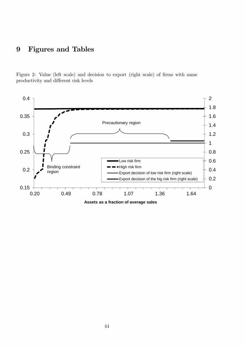
9 Figures and Tables

Figure 2: Value (left scale) and decision to export (right scale) of firms with same

productivity and different risk levels

0

0.2

0.4

0.6

0.8

1

1.2

1.4

1.6

1.8

2

0.15

0.2

0.25

0.3

0.35

0.4

0.20 0.49 0.78 1.07 1.36 1.64

Assets as a fraction of average sales

Low risk firm

High risk firm

Export decision of low risk firm (right scale)

Export decision of the hig risk firm (right scale)

Precautionary region

Binding constraint region

44

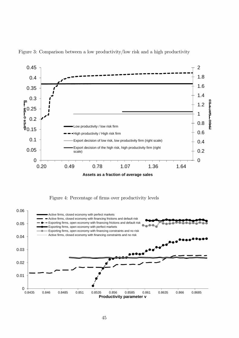
Figure 3: Comparison between a low productivity/low risk and a high productivity

0

0.2

0.4

0.6

0.8

1

1.2

1.4

1.6

1.8

2

0

0.05

0.1

0.15

0.2

0.25

0.3

0.35

0.4

0.45

0.20 0.49 0.78 1.07 1.36 1.64

Export decision

Value of the firm

Assets as a fraction of average sales

Low productivity / low risk firm

High productivity / High risk firm

Export decision of low risk, low productivity firm (right scale)

Export decision of the high risk, high productivity firm (rightscale)

Figure 4: Percentage of firms over productivity levels

0

0.01

0.02

0.03

0.04

0.05

0.06

0.8435 0.846 0.8485 0.851 0.8535 0.856 0.8585 0.861 0.8635 0.866 0.8685Productivity parameter v

Active firms, closed economy with perfect marketsActive firms, closed economy with financing frictions and default riskExporting firms, open economy with financing frictions and default riskExporting firms, open economy with perfect marketsExporting firms, open economy with financing constraints and no riskActive firms, closed economy with financing constraints and no risk

45

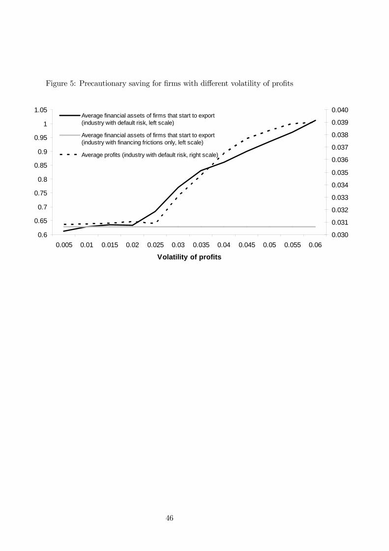
Figure 5: Precautionary saving for firms with different volatility of profits

0.6

0.65

0.7

0.75

0.8

0.85

0.9

0.95

1

1.05

0.005 0.01 0.015 0.02 0.025 0.03 0.035 0.04 0.045 0.05 0.055 0.06

Volatility of profits

0.030

0.031

0.032

0.033

0.034

0.035

0.036

0.037

0.038

0.039

0.040Average financial assets of firms that start to export(industry with default risk, left scale)

Average financial assets of firms that start to export(industry with financing frictions only, left scale)

Average profits (industry with default risk, right scale)

46

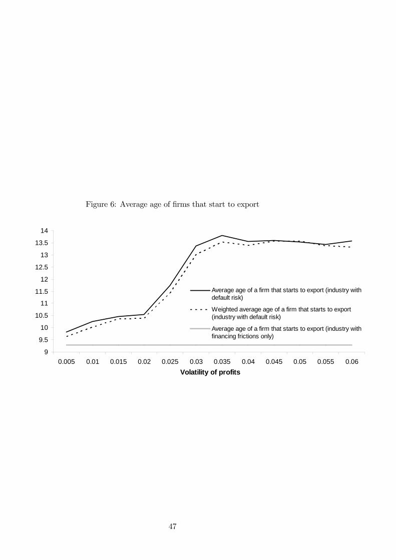
Figure 6: Average age of firms that start to export

9

9.5

10

10.5

11

11.5

12

12.5

13

13.5

14

0.005 0.01 0.015 0.02 0.025 0.03 0.035 0.04 0.045 0.05 0.055 0.06

Volatility of profits

Average age of a firm that starts to export (industry withdefault risk)

Weighted average age of a firm that starts to export(industry with default risk)

Average age of a firm that starts to export (industry withfinancing frictions only)

47

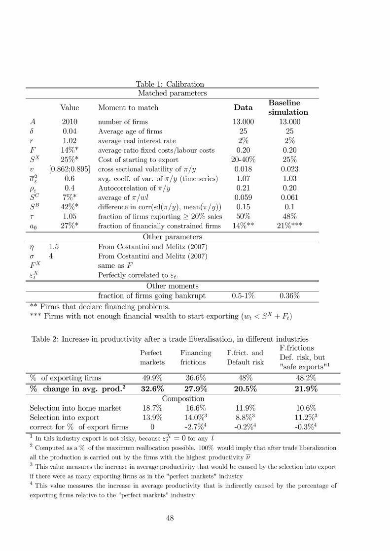
Table 1: CalibrationMatched parameters

Value Moment to match DataBaseline

simulation

2010 number of firms 13.000 13.000

0.04 Average age of firms 25 25

1.02 average real interest rate 2% 2%

14%* average ratio fixed costs/labour costs 0.20 0.20

25%* Cost of starting to export 20-40% 25%

[0.862;0.895] cross sectional volatility of 0.018 0.023

2 0.6 avg. coeff. of var. of (time series) 1.07 1.03

0.4 Autocorrelation of 0.21 0.20

7%* average of 0.059 0.061

42%* difference in corr(sd() mean()) 0.15 0.1

1.05 fraction of firms exporting ≥ 20% sales 50% 48%

0 27%* fraction of financially constrained firms 14%** 21%***

Other parameters

1.5 From Costantini and Melitz (2007)

4 From Costantini and Melitz (2007)

same as

Perfectly correlated to

Other moments

fraction of firms going bankrupt 0.5-1% 0.36%

** Firms that declare financing problems.

*** Firms with not enough financial wealth to start exporting ( + )

Table 2: Increase in productivity after a trade liberalisation, in different industries

Perfect

markets

Financing

frictions

F.frict. and

Default risk

F.frictions

Def. risk, but

"safe exports"1

% of exporting firms 49.9% 36.6% 48% 48.2%

% change in avg. prod.2 32.6% 27.9% 20.5% 21.9%

Composition

Selection into home market 18.7% 16.6% 11.9% 10.6%

Selection into export 13.9% 14.0%3 8.8%3 11.2%3

correct for % of export firms 0 -2.7%4 -0.2%4 -0.3%4

1 In this industry export is not risky, because = 0 for any 2 Computed as a % of the maximum reallocation possible. 100% would imply that after trade liberalization

all the production is carried out by the firms with the highest productivity 3 This value measures the increase in average productivity that would be caused by the selection into export

if there were as many exporting firms as in the "perfect markets" industry4 This value measures the increase in average productivity that is indirectly caused by the percentage of

exporting firms relative to the "perfect markets" industry

48

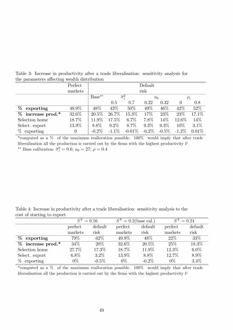
Table 3: Increase in productivity after a trade liberalisation: sensitivity analysis for

the parameters affecting wealth distribution

Perfect

markets

Default

risk

Base∗∗ 2 0 05 07 0.22 0.32 0 0.8

% exporting 49.9% 48% 43% 50% 49% 46% 42% 52%

% increase prod.* 32.6% 20.5% 26.7% 15.3% 17% 23% 23% 17.1%

Selection home 18.7% 11.9% 17.5% 6.7% 7.8% 14% 12.6% 14%

Select. export 13.9% 8.8% 9.2% 8.7% 9.3% 9.3% 10% 3.1%

% exporting 0 -0.2% -1.1% -0.01% -0.2% -0.5% -1.2% 0.01%

*computed as a % of the maximum reallocation possible. 100% would imply that after trade

liberalization all the production is carried out by the firms with the highest productivity ∗∗ Base calibration: 2 = 06; 0 = 27; = 04

Table 4: Increase in productivity after a trade liberalisation: sensitivity analysis to the

cost of starting to export

= 016 = 02(base cal.) = 024

perfect

markets

default

risk

perfect

markets

default

risk

perfect

markets

default

risk

% exporting 79% 62% 49.9% 48% 22% 33%

% increase prod.* 34% 20% 32.6% 20.5% 25% 18.3%

Selection home 27.7% 17.3% 18.7% 11.9% 12.3% 6.0%

Select. export 6.8% 3.2% 13.9% 8.8% 12.7% 8.9%

% exporting 0% -0.5% 0% -0.2% 0% 3.4%

*computed as a % of the maximum reallocation possible. 100% would imply that after trade

liberalisation all the production is carried out by the firms with the highest productivity

49

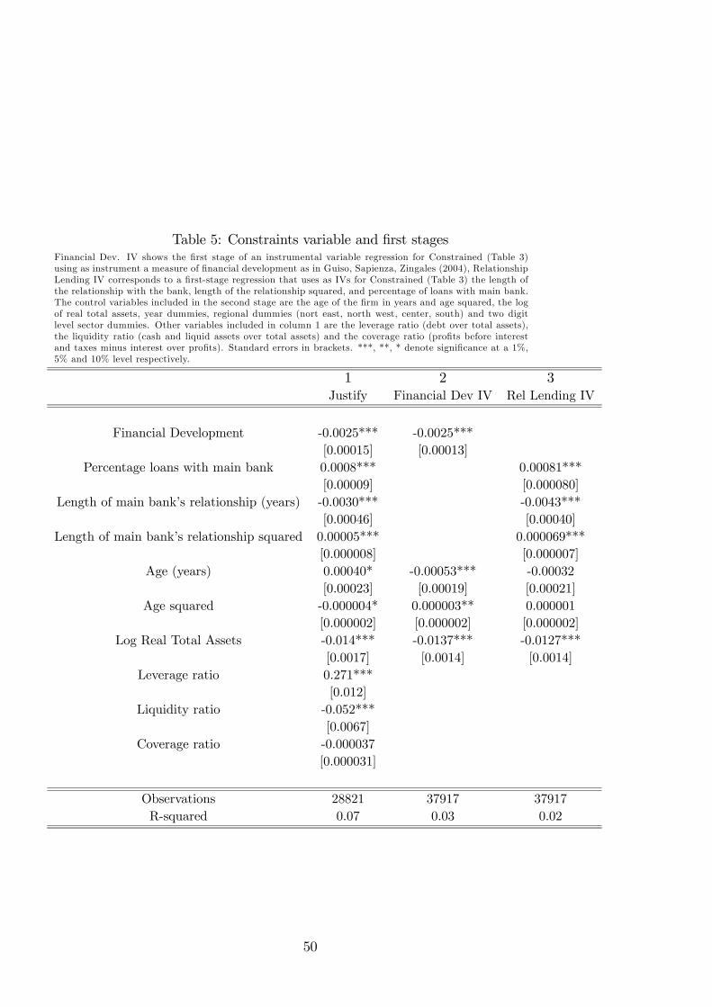
Table 5: Constraints variable and first stagesFinancial Dev. IV shows the first stage of an instrumental variable regression for Constrained (Table 3)

using as instrument a measure of financial development as in Guiso, Sapienza, Zingales (2004), Relationship

Lending IV corresponds to a first-stage regression that uses as IVs for Constrained (Table 3) the length of

the relationship with the bank, length of the relationship squared, and percentage of loans with main bank.

The control variables included in the second stage are the age of the firm in years and age squared, the log

of real total assets, year dummies, regional dummies (nort east, north west, center, south) and two digit

level sector dummies. Other variables included in column 1 are the leverage ratio (debt over total assets),

the liquidity ratio (cash and liquid assets over total assets) and the coverage ratio (profits before interest

and taxes minus interest over profits). Standard errors in brackets. ***, **, * denote significance at a 1%,

5% and 10% level respectively.

1 2 3

Justify Financial Dev IV Rel Lending IV

Financial Development -0.0025*** -0.0025***

[0.00015] [0.00013]

Percentage loans with main bank 0.0008*** 0.00081***

[0.00009] [0.000080]

Length of main bank’s relationship (years) -0.0030*** -0.0043***

[0.00046] [0.00040]

Length of main bank’s relationship squared 0.00005*** 0.000069***

[0.000008] [0.000007]

Age (years) 0.00040* -0.00053*** -0.00032

[0.00023] [0.00019] [0.00021]

Age squared -0.000004* 0.000003** 0.000001

[0.000002] [0.000002] [0.000002]

Log Real Total Assets -0.014*** -0.0137*** -0.0127***

[0.0017] [0.0014] [0.0014]

Leverage ratio 0.271***

[0.012]

Liquidity ratio -0.052***

[0.0067]

Coverage ratio -0.000037

[0.000031]

Observations 28821 37917 37917

R-squared 0.07 0.03 0.02

50

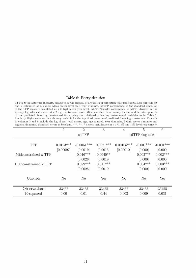
Table 6: Entry decisionTFP is total factor productivity, measured as the residual of a translog specification that uses capital and employment

and is estimated at a 2 digit Ateco sector level on 3 year windows. sdTFP corresponds to the standard deviation

of the TFP measure calculated at a 2 digit sector-year level. sdTFP/logsales corresponds to sdTFP divided by the

average log sales calculated at a 2 digit sector-year level. Midconstrained is a dummy for the middle third quantile

of the predicted financing constrained firms using the relationship lending instrumental variables as in Table 2.

Similarly Highconstrained is a dummy variable for the top third quantile of predicted financing constraints. Controls

in columns 3 and 6 include the log of real total assets, age, age squared, year dummies, 2 digit sector dummies and

regional dummies. Standard errors in brackets. ***, **. * denote significance at a 1%, 5% and 10% level respectively.

1 2 3 4 5 6

sdTFP sdTFP/log sales

TFP 0.0123*** -0.0051*** 0.0071*** 0.00105*** -0.001*** -0.001***

[0.00097] [0.0019] [0.0015] [0.00010] [0.000] [0.000]

Midconstrained x TFP 0.016*** 0.0040** 0.003*** 0.002***

[0.0026] [0.0019] [0.000] [0.000]

Highconstrained x TFP 0.029*** 0.011*** 0.004*** 0.003***

[0.0025] [0.0019] [0.000] [0.000]

Controls No No Yes No No Yes

Observations 33455 33455 33455 33455 33455 33455

R-squared 0.00 0.01 0.44 0.003 0.009 0.031

51

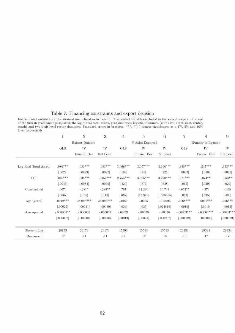
Table 7: Financing constraints and export decisionInstrumental variables for Constrained are defined as in Table 1. The control variables included in the second stage are the age

of the firm in years and age squared, the log of real total assets, year dummies, regional dummies (nort east, north west, center,

south) and two digit level sector dummies. Standard errors in brackets. ***, **, * denote significance at a 1%, 5% and 10%

level respectively.

1 2 3 4 5 6 7 8 9

Export Dummy % Sales Exported Number of Regions

OLS IV IV OLS IV IV OLS IV IV

Financ. Dev Rel Lend. Financ. Dev Rel Lend. Financ. Dev Rel Lend.

Log Real Total Assets 086*** 081*** 083*** 3.066*** 3.057*** 3.166*** 358*** 347*** 353***

[0022] [0029] [0027] [199] [241] [225] [0082] [010] [0095]

TFP 048*** 038*** 0354*** 2.755*** 3.696*** 3.220*** 071*** 074** 053**

[0046] [0084] [0068] [420] [776] [628] [017] [029] [024]

Constrained 0070 -281* -288** 707 12.230 10.743 -062** -379 -468

[0067] [155] [113] [637] [13.975] [1038485] [024] [535] [400]

Age (years) .0012*** 00098*** 00095*** -0167 -0065 -010705 0068*** 0067*** 006***

[00027] [00031] [00030] [024] [025] [024819] [0010] [0010] [0011]

Age squared -.000005** -000003 -000003 -00021 -00029 -00026 -00003*** -00003*** -00003***

[.000002] [000003] [000003] [00019] [00021] [000207] [000009] [000009] [000009]

Observations 29173 29173 29173 15593 15593 15593 29334 29334 29334

R-squared 17 11 11 14 12 13 18 17 17

52

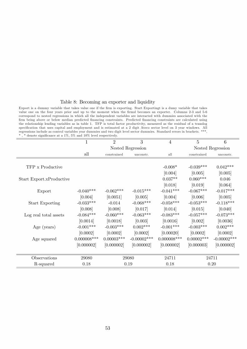
Table 8: Becoming an exporter and liquidityExport is a dummy variable that takes value one if the firm is exporting. Start Exportingt is a dumy variable that takes

value one on the four years prior and up to the moment when the firmsl becomes an exporter. Columns 2-3 and 5-6

correspond to nested regressions in which all the independent variables are interacted with dummies associated with the

firm being above or below median predicted financing constraints. Predicted financing constraints are calculated using

the relationship lending variables as in table 1. TFP is total factor productivity, measured as the residual of a translog

specification that uses capital and employment and is estimated at a 2 digit Ateco sector level on 3 year windows. All

regressions include as control variables year dummies and two digit level sector dummies. Standard errors in brackets. ***,

* , * denote significance at a 1%, 5% and 10% level respectively.

1 2 3 4 5 6

Nested Regression Nested Regression

all constrained unconstr. all constrained unconstr.

TFP x Productive -0.008* -0.039*** 0.042***

[0.004] [0.005] [0.005]

Start Export.xProductive 0.037** 0.060*** 0.046

[0.018] [0.019] [0.064]

Export -0.040*** -0.062*** -0.015*** -0.041*** -0.067*** -0.017***

[0.004] [0.0051] [0.005] [0.004] [0.006] [0.005]

Start Exporting -0.033*** -0.014 -0.068*** -0.058*** -0.053*** -0.118***

[0.008] [0.008] [0.017] [0.014] [0.015] [0.040]

Log real total assets -0.084*** -0.060*** -0.063*** -0.083*** -0.057*** -0.073***

[0.0014] [0.0018] [0.003] [0.0016] [0.002] [0.0036]

Age (years) -0.001*** -0.003*** 0.002*** -0.001*** -0.003*** 0.002***

[0.0002] [0.0002] [0.0002] [0.00020] [0.0002] [0.0002]

Age squared 0.000008*** 0.00003*** -0.00002*** 0.000008*** 0.00002*** -0.00002***

[0.000002] [0.000002] [0.000002] [0.000002] [0.000003] [0.000002]

Observations 29080 29080 24711 24711

R-squared 0.18 0.19 0.18 0.20

53

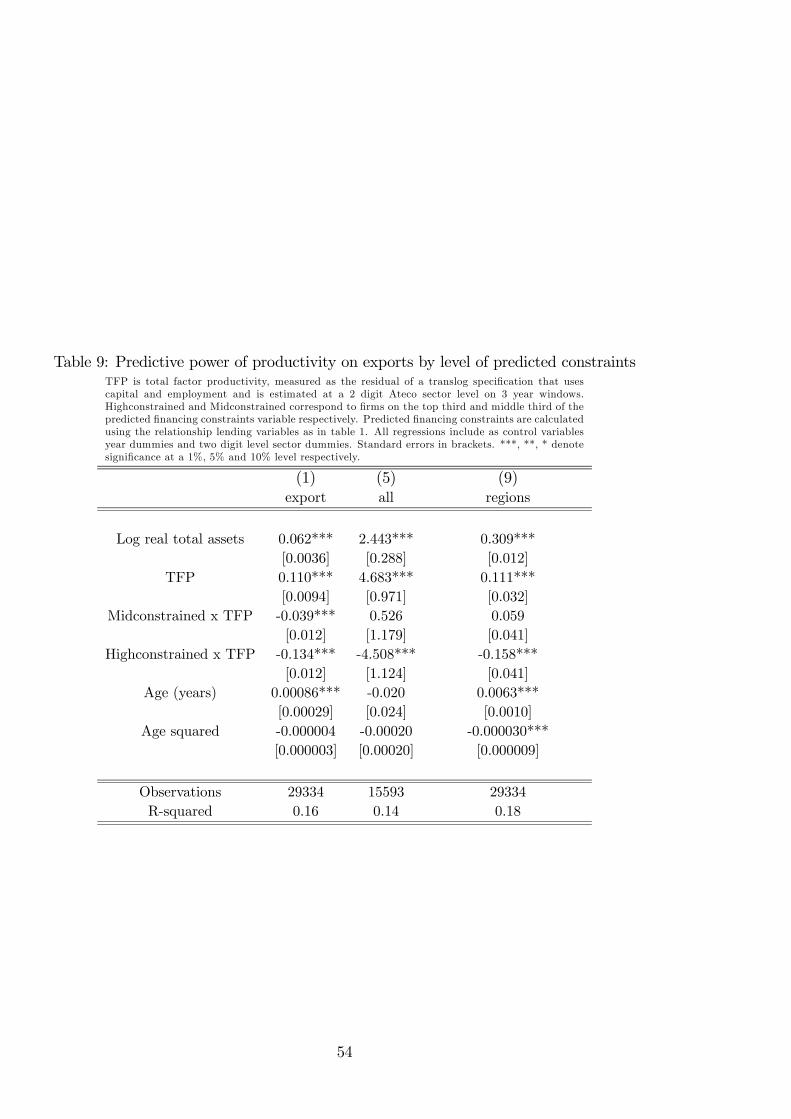
Table 9: Predictive power of productivity on exports by level of predicted constraintsTFP is total factor productivity, measured as the residual of a translog specification that uses

capital and employment and is estimated at a 2 digit Ateco sector level on 3 year windows.

Highconstrained and Midconstrained correspond to firms on the top third and middle third of the

predicted financing constraints variable respectively. Predicted financing constraints are calculated

using the relationship lending variables as in table 1. All regressions include as control variables

year dummies and two digit level sector dummies. Standard errors in brackets. ***, **, * denote

significance at a 1%, 5% and 10% level respectively.

(1) (5) (9)

export all regions

Log real total assets 0.062*** 2.443*** 0.309***

[0.0036] [0.288] [0.012]

TFP 0.110*** 4.683*** 0.111***

[0.0094] [0.971] [0.032]

Midconstrained x TFP -0.039*** 0.526 0.059

[0.012] [1.179] [0.041]

Highconstrained x TFP -0.134*** -4.508*** -0.158***

[0.012] [1.124] [0.041]

Age (years) 0.00086*** -0.020 0.0063***

[0.00029] [0.024] [0.0010]

Age squared -0.000004 -0.00020 -0.000030***

[0.000003] [0.00020] [0.000009]

Observations 29334 15593 29334

R-squared 0.16 0.14 0.18

54