TAX EVASION ACROSS INDUSTRIES: SOFT CREDIT EVIDENCE FROM GREECE

NIKOLAOS ARTAVANIS ADAIR MORSE MARGARITA TSOUTSOURA

Virginia Polytechnic Institute and State University

University of Chicago, Booth School of Business,

UC Berkeley, Haas School of Business and NBER

University of Chicago, Booth School of Business

September 2012

Abstract

We begin with the new observation that banks lend to tax-evading individuals based on the bank's perception of true income. This insight leads to a novel approach to estimate tax evasion from private-sector adaptation to semiformality. We use household microdata from a large bank in Greece and replicate bank models of credit capacity, credit card limits, and mortgage payments to infer the bank’s estimate of individuals’ true income. We estimate a lower bound of 28 billion euros of unreported income for Greece. The foregone government revenues amount to 31 percent of the deficit for 2009. Primary tax-evading occupations are doctors, engineers, private tutors, accountants, financial service agents, and lawyers. Testing the industry distribution against a number of redistribution and incentive theories, our evidence suggests that industries with low paper trail and industries supported by parliamentarians have more tax evasion. We conclude by commenting on the property right of informal income.

*Corresponding Authors: Adair Morse; email: adair.morse@chicagobooth.edu. Margarita Tsoutsoura; email: tsoutsoura@chicagobooth.edu. We are grateful to the anonymous bank that supplied the data. We are thankful for helpful comments to Laurent Bach, Loukas Karabarbounis, Elias Papaioannou, Dina Pomeranz, Amit Seru, Annette Vissing-Jorgensen, Luigi Zingales, and seminar participants at Chicago Booth, Berkeley Haas, INSEAD, Catholica Lisbon School of Business, London Business School, NOVA School of Business, UBC, NBER Corporate Finance Summer Institute, NBER Public Economic meeting, IDC Summer Finance Conference, CEPR Gerzensee Summer Symposium, 8th Csef-Igier Symposium, Booth-Deutschebank Symposium and the Political Economy in the Chicago area conference This research was funded in part by the Fama-Miller Center for Research in Finance, the Polsky Center for Entrepreneurship at the University of Chicago, Booth School of Business, and the Goult Faculty Research Endowment. Tsoutsoura gratefully acknowledges financial support from the PCL Faculty Research Fund at the University of Chicago, Booth School of Business

1 Introduction

As countries develop, many transactions that once would have occurred in the shadow economy

move to formal establishments, financed by formal banking. A little-observed fact is that this

transition does not necessarily bring the formalization of income. In particular, in countries

with generous social services, an environment of semiformality can emerge, in which individuals

remain registered taxpayers, to receive public benefits, but do not declare all of their income

to tax authorities. According to the Enterprise Surveys of the World Bank, 52% of companies

across all countries do not report all income to tax authorities, which is perhaps not a surprising

figure given the size of the black market in emerging and less developed countries. What is

surprising is that this figure is not much smaller (36%) for Europe. Very little is known about

semiformality and its impact on individual choices and production at large, although this setting

anecdotally describes a good portion of the world.

As an emphasis of this point, consider the contrast between the studies of tax evasion and in-

formality. Tax evasion studies primarily focus on incentives to evade and enforce.1 By contrast,

studies of informality, usually in developing countries, consider ineffi ciencies in production, hu-

man capital accumulation, and implications to industry composition.2 A goal of this paper is

to bridge some of this gap by studying the industry distribution of semiformal income. We

do so in the setting of Greece, where understanding the distribution of tax evasion may be

of first order to current policies, but also where we can assemble data to understand industry

characteristics that facilitate the perpetuation of tax evasion.

A second goal is to bring to light the connection between tax evasion and bank credit, which

we then use for a methodological contribution. In the informality literature, a standard assump-

tion is that informal businesses do not have access to formal capital markets. Semiformality,

however, need not imply that the private sector excludes individuals from credit access. Banks

adapt to the culture of semiformality and provide credit to individuals based on their inference

1Andreoni, Erard, and Feinstein (1998) and Slemrod and Yitzaki (2002) offer a comprehensive review of the

literature. The foundations for the empirical work can be found in Allingham and Sandmo (1972), Pencavel

(1979), Cowel (1985), and many others.2For example, La Porta and Shleifer (2008) contrast formal and informal firms in developing countries, finding

support for the dual economy view that informal firms are just not the equivalent of formal ones in capital use,

human capital, access to finance, and overall market and customer base. Banerjee and Duflo (2005) and Restuccia

and Rogerson (2008) discuss and Hseih and Klenow (2009) test the output differential for (informal) firms with

lower marginal product of labor and capital.

1

of true income.3 An interesting observation about credit given on taxed-evaded income is that

the process dampens Stiglitz-Weiss (1981) credit rationing that would have occurred because

of the unobservability of semiformal income. Thus, the fact that banks make an inference as

to true income increases the overall pie of credit issued. Because the income inference is soft

information, we call this expansion of credit, soft credit.

Before discussing our methodology, we motivate our study with a table illustrating bank

adaptation and soft credit at work. The data are from a large Greek bank, covering tens

of thousands applications by individuals for credit products.4 Columns 1 and 2 show the

monthly declared income and monthly payments on household credit products for self-employed

individuals across different industries, and column 3 presents the ratio of payments-to-income.

On average, self-employed Greeks spend 82% of their monthly reported income servicing debt.

To put this number in perspective, the standard practice in consumer finance (in the United

States as well as Greece) is to never lend to borrowers such that loan payments are greater than

30% of monthly income. And that is the upper limit.

The point of this table is to establish that adaptation is happening and to motivate how we

use bank data to speak to tax evasion. A number of banks in southern Europe told us point

blank that they have adaptation formulas to adjust clients’reported income to the bank’s best

estimate of true income, and furthermore, that these adjustments are specific to occupations.

Table 1 shows evidence of adaptation in practice. Take the examples of lawyers, doctors,

financial services, and accountants. In all of these occupations, the self-employed are paying

over 100% of their reported income flows to debt servicing on consumer loans. Moreover, this

lending is no more risky; the default rate (column 4) on loans to lawyers, doctors, financial

services, and accountants is no higher than on loans to people in occupations who on average

are less burdened with consumer debt payments. The correlation between defaults and the

ratio of debt payments to income is a small negative number.

The innovation of using bank data to estimate tax evasion is itself a contribution. Our

insight is that because the private sector adapts to a culture of tax evasion, private sector data

offer a window into the magnitude of, distribution of, and motivation for tax evasion.

Our private sector data method adds to the list of approaches to estimate tax evasion. In par-

3Harberger (2006) discusses customs tax evasion and institutional adaptation. We borrow the term adaptation

from him and apply it to bank actions.4The data section later describes the data in detail. For purposes here, it is a suffi ciently large dataset weighted

to the population distribution of Greece. In this illustrative table, we use mortgage applications and consumer

credit product applications for non-homeowners. (We discarded consumer credit products for homeowners since

we could not determine the interest rate and maturity on mortgage debt outstanding.)

2

ticular, the private data methodology offers an opportunity to uncover hidden income in places

where using the other methods might prove diffi cult. For example, the most direct method of

estimating tax evasion is via audits of tax returns (Klepper and Nagin (1989), Christian (1994),

Feinstein (1999), Kleven, Knudsen, Kreiner, Pedersen and Saez (2011)). Although audit data

are very detailed and appealing, the process of doing wide-ranging audits and collecting the

data is an expensive proposition to many places outside the U.S. and northern Europe.

The most frequently used method in the literature is via indirect estimates from observed

expenditure data, building on Pissarides and Weber (1989), who use food expenditure survey

data to estimate the underreporting of British self-employed. The consumption-based method-

ology has been applied in a host of settings (Lyssiotou, Pashardes and Stengos (2004), Feldman

and Slemrod (2007), Gorodnichenko, Martinez-Vazquez and Sabirianova (2009), Braguinsky,

Mityakov and Liscovich (2010)).5Although recently Hurst, Li, and Pugsley (2011) show that

people underreport their income in surveys, adding to the selection complications of the survey

method, our methodological contribution is about applicability, not necessarily about improv-

ing on selection issues. The private data method provides a way to estimate tax evasion in

countries where the design and implementation of a population-representative survey would be

too costly and diffi cult. Furthermore, by using banking data, we have access to a rich set of hard

and soft information that a survey would be hard to capture but are important determinants

of the tax evading behavior.

One of the ten largest banks in Greece provided us with individual-level application and

performance data from credit products — credit cards, term loans, mortgages, and overdraft

facilities. The application data include rich information on reported income, total debt out-

standing, occupation, employment status (self-employed or wage earner), credit history, and

demographics. We know the zip code of the borrowers, which allows us to construct soft infor-

mation variables including local economy growth and proxies for wealth and the variability of

income.

Our approach to estimate true income from bank data is based on a causal relationship that

individuals must have income (or flows from wealth) to service debt. When individuals apply

for bank credit or a payment product, a bank offi cer applies a decision model to determine

5A separate literature relies on macroeconomic approaches to estimate the size of the black economy. The

most common approaches are consumption methods (e.g., as in the electricity approach of Lacko (1999)) and

the currency demand approach (Cagan (1958), Tanzi (1983)). These methods are best suited to estimate the

size of the shadow economy, which emcompass but are not specific to income tax evasion. Sneider (2002) gives

an overview of these methods, discussing their benefits and limitations and higlighting differences between the

black economy estimates and income tax evasion.

3

whether and to what extent the individual qualifies. These credit decision models utilize a host

of risk- and wealth-profiling variables, but by far the most important factor in determining

credit worthiness is true income. True income is, however, not observable, and so the bank

applies adaptation rules to offer soft credit on their best estimate of true income, given the

reported income.

Our identification relies on the standard assumption in the tax evasion literature that re-

ported income is equal to true income for wage earners.6 We thus estimate the sensitivity of

credit offered to income off the wage earners. Since one needs a certain amount of cash mechan-

ically to service debt, the true income-to-credit relationship should be the same for individuals

only differing as to self-employment or not. (Self-employment itself may imply different risk

and income processes, an issue we take up by using fixed effects for self-employment crossed

with occupation and with soft information variables.) Since we know that the structure of the

bank’s adaptation model is occupation-specific, we can estimate what the true income must be

to support the level of credit offered by occupation. Our main inference outcome is a set of

reported income multipliers (and the implied tax evasion in euros) specific to each industry.

We apply our method in a variety of bank credit decisions: the credit capacity decision for

a constrained consumer, the credit limit for new credit card products, and the monthly pay-

ments affordable for a mortgage borrower. We choose these settings to focus in on loan product

customers whose credit application outcome is determined by the bank (supply determined).

Furthermore we apply our analysis to this variety of settings to produce population represen-

tative results. For example, on the first count, we have many applications in which the amount

of loan requested is lower than the amount received. On the latter issue of representativeness,

we argue that our credit card sample is close to being representative of the population, since

most of Greek households took out credit cards, for the first time, in our sample period after

innovations in payment systems with the euro implementation. In order to combine the infor-

mation we obtain from the different settings, but also to take into account the precision of the

various credit product estimates, we combine the estimates using precision weighting.

We find 28 billion euros in evaded taxable income for 2009, just for the self-employed.

GDP for 2009 was 235 billion euros, and the tax base in Greece was 98 billion euros; thus

our magnitude is very meaningful. At the tax rate of 40%, the foregone tax revenues would

account for 31% of the budget deficit shortfall in 2009 (or 48% for 2008). We find that on

average the true income of self-employed is 1.92 times their reported income.7 These estimates

6The assumption that wage earners do not tax evade is incorrect on average. Side jobs are commonplace in

many occupations. This possibility biases down our estimates.7To put some perspective on the magnitudes, Pissarides and Weber (1989) find that on average the true

4

are conservative in that our estimates may reflect a haircut taken by the bank on how much

soft credit they issue off their inference of true income and in that our estimates are biased

downwards to the extent that wage earners tax evade in Greece. Geographically, our findings

line up perfectly with recent attention in the popular press concerning the ownership of Porsche

Cayennes in Greek towns.

The main goal of our estimation is to study the industry incidence of tax evasion. We

find a high tax evasion multiple for doctors, engineers, private tutors, financial services agents,

accountants, and lawyers, consistently across different credit models.

We turn to making sense of the industry distribution. We find no evidence that the govern-

ment is subsidizing either areas of local economic growth or industries offering apprentice-like

training to unskilled workers. Turning to incentive stories, we investigate enforcement using

detailed data by tax authority offi ces (which are very local in Greece). Our data tell an in-

teresting story of enforcement, but the incentives of enforcement do not explain the industry

distribution of tax evasion.

Instead, we find strong evidence supporting that of Kleven, Knudsen, Kreiner, Pedersen and

Saez (2011) that enforcement involves information. When industries use inputs and produce

outputs with paper trails, they are less likely to tax evade. Our industry distribution of tax

evasion is very consistent with paper trail survey scores we collect from professional business

students in Greece.

We also find evidence of a political economy story. We were motivated to pursue this

story by the failure of a legislative bill in the Greek Parliament in 2010. The idea of the

bill was to mandate tax audits for reported income below a minimum amount, targeted at

eleven select occupations. The occupations line up almost perfectly with our results: doctors,

dentists, veterinarians, lawyers, architects, engineers, topographer engineers, economists, firm

consultants and accountants. Our political economy story is that parliamentarians lacking the

willpower to pass tax reform may have personal incentive related to their industry associations,

which are very strong in Greece. We find that indeed the occupations represented in Parliament

are very much those which tax evade, even beyond lawyers. Half of non-lawyer parliamentarians

are in the top three tax evading industries, and nearly a supermajority in the top four evading

industries.

Our study concludes with thoughts on a property rights view of soft credit. The fact that

income of self-employed in Great Britain is 1.55 times their reported income. Feldman and Slemrod (2007) use

the relationship between reported charitable contributions and reported income, and find that in US tax evasion

among self-employed, nonfarm small-business and farm income are 1.54, 4.54 and 3.87 times reported income,

respectively.

5

banks give an entitlement to informal income provides a property right that allows individuals to

use borrowing more optimally to smooth lifetime consumption or overcome shocks. We cannot

pursue this welfare argument in this paper. However, because the observation that banks adapt

to semiformality by issuing soft credit is a new one, we conclude with thoughts on whether the

haircut banks impose on hidden income in their lending should be zero, one, or somewhere in

between, given a norm of tax evasion in the culture and the political willpower of a country.

The remainder of the paper is as follows. Section 2 introduces our rich bank and tax

authority data, and provides summary statistics. Section 3 lays out our methodology. Section

4 reports results. Section 5 discusses validity, interprets magnitudes at the economy-level, and

lays out the incidence of tax evasion. Section 6 investigates theories to make sense of the

distribution of tax evasion across industries. Section 7 discusses welfare and concludes.

2 Data

Our main data are proprietary files covering 2003-2010 from one of the ten large Greek banks,

which together account for eighty percent of the market share. The bank has tens of thousands

of customers, with branches across the country. The dataset is the universe of applications

for consumer credit products and mortgages, both approved and rejected. Consumer credit

products include term loans, credit lines, credit cards, overdraft facilities, appliance loans, and

refinancings.

Our dataset includes every piece of hard information that the bank uses in its credit scoring

model. Administrative data provide the date of the application, the branch offi ce, the purpose of

the loan, the requested and approved amounts and durations, the debt outstanding at this bank,

and the total debt outstanding elsewhere. Demographic data are marital status and number of

children. Permanent income variables include reported income (as reported in the tax return

and verified by the bank), occupation, employment type (wage worker or self-employed), age,

and co-applicant or spouse income. Credit worthiness variables include years in job, years in

address, homeownership, the length of the relationship with the bank, deposit holdings in the

bank, and overall status of the relationship with the bank (new customer, existing customer in

good standing, existing customer in bad standing). We label a customer to be in bad standing if

he is delinquent in one of his loans with the bank in the last 6 months by using the performance

dataset of these accounts, which includes monthly installment payments, balance outstanding,

and interest rate. Appendix A2 provides detailed information on the credit history construction.

Although we have the universe of applications for consumer loans, our analysis focuses on

6

four subsamples with dual aims in mind. The first aim is to isolate the supply side of credit

by identifying situations in which the bank (and not the applicant) makes decision regarding

the level of the loan product observed. The first sample, the constrained sample, contains all

consumer loan applicants whose requested loan amount is greater than the approved amount

plus overdraft applicants with less than 1,000 euros on deposit.8 The time frame for the

constrained sample analysis is January, 2003-October, 2009, when the crisis began in earnest

in Greece. The banks fundamentally changed their loan processes beginning at this point as

liquidity and solvency issues became acutely more pressing.

Crisis lending itself motivates our second sample. Our refinancing sample is the set of

borrowers refinancing their debts during the crisis (October, 2009 - December, 2010), reflecting

a new loan product code for refinancings introduced by the bank during 2009.

In the case of these first two samples, our dependent variable is the bank’s decision as to the

overall credit capacity of the customer, defined as total debt outstanding immediately following

the loan application decision. Note that the bank records data on all debt, including that from

other financial institutions. Our model for the first two samples assumes that the bank treats

all debt capacity as having the same relationship to income, once we control for shifters like

homeownership. We offer different sample models that do not need this assumption, partially

as robustness to this assumption.

The third sample, the credit card sample, is that of credit card applicants from new bank

customers. In the years that we analyze, many innovations in the use of payment systems

emerged in Greece, with credit cards in particular becoming increasingly used and needed as

means of payment. Most people did not have a need for a credit card until the implementation

of euro payment systems after the entrance into the Eurozone in 2002. The purpose of the

credit card sample is to select individuals who may be independent of the need for bank loans,

thus being very population representative. Another benefit of the credit card sample is that we

identify off a different dependent variable, namely the credit card limit, not overall debt. The

credit card limit on new credit cards is not usually a function of the borrowing wanted at that

instance. Thus, by looking at credit card limits, we identify soft credit off a different model,

8The constrained sample does not include mortgages and car loans. The bank keeps car loans separate accounts

withouth identifiers. Thus we exclude them in the analysis because we cannot properly match individuals. We

focus on mrtgages subsequently. Overdraft facilities are issued either because the person in in distress and

requests some slack or, perhaps inadvertantly, when a new customer opens a checking account or some other

banking product. We filter based on individuals having 1,000 euros on deposit as a way to filter out individuals

who have precautionary savings and are likely to be opening the overdraft as a part of opening or changing their

banking products.

7

with more population representative users, than total credit capacity of constrained individuals.

The disadvantage of this sample is that we have fewer observations.

The final sample is the mortgage sample. Individuals who take out a mortgage generally

choose to buy as much house as their economic situation supports; thus, post-mortgage, these

individuals are usually close to or at the level of payments that their incomes support. The

mortgage sample has the appealing characteristic, reflecting the second goal of subsampling of

being nationally representative, of not sampling on predominately ex ante negative net worth

individuals. Home buyers are of all spectrums of workers in Greece, where 80% of households

eventually end up owning homes. The limitation of this sample is size. We only have mortgage

files starting in 2006 and cut the sample at the crisis. Beyond the time period, the yearly files

are a much smaller dataset, and we face limits in our empirical design, which uses very detailed

(zip code-occupation level) identification.

The decision variable for the mortgage sample is the monthly payments of approved mort-

gage. Mortgage lenders have standard rules regarding this formula; for instance, mortgage

payments should not be more that 30% of monthly income. Thus, payments is a natural vari-

able, which we calculate with the maturity and interest rate of the loan, taking account of any

teaser rate period that we observe in the performance files. Again, using a different outcome

decision is a nice robustness check on our estimates.

We supplement the bank data with detailed zip code level data from the Greek tax authority.

For every zip code, we have deciles of income for all tax filers as well as their classification in

four employment categories: Merchants and Small Business Owners, Agriculture, Wage Earners

and Self-Employed. To illuminate the detail of these data, for a population of 6 million tax

filers, we have a breakdown of the number of filers and total income by 1,569 different zip codes,

10 national deciles of income and 4 professions. Each of the nearly 63,000 cells does not have

many people observations in it.

We use the detailed income deciles per zip code data from the tax authorities to weight

our sample to the population, aggregating to the quintile of income, four professions, and nine

meta-prefecture level. For our analysis, we exclude students, pensioners and unemployed, since

our goal is to focus on the active workforce.

We also use the fine detail of these data to construct soft information variables and proxies.

We construct local income growth as per capital annual income growth of the prior year at

the level of the zip code crossed with the four occupation-levels and the ten income decile.

(The tax authority defines these national income ‘deciles’, which are stationary year-to-year

and national.) We also calculate a measure of the variability of this income growth, which is

8

the standard deviation of the growth of income in the cell.9 These measures serve both as soft

information proxies for individual income growth used by the bank and as direct measures of

the soft information of local conditions.

We also proxy for the wealth of individuals in the zip code and occupation level in three

ways. First, the tax authority provided us with presumed real estate values by building block.

We take the median of these values to collapse to the zip code level. Second, using the bank’s

vehicle loans file, we create an alternative measure of average car values and average loan-to-

values of new cars by zip code. The loan-to-value measure should capture a wealth effect on

downpayments (Adams, Einav, and Levin, 2009).

Table 2 presents the mean statistics for the variables by sample and by employment status.

The definitions of the variables are given in the Data Appendix A1. It is worth noting that

credit capacity, credit card limits, and mortgage payments are higher for the self-employed

than wage workers. The reported income levels for the mortgage and refinancing sample are

much lower, while in the constraint and credit card sample are slightly higher. So even in a

naive comparison of average income and credit capacity, the data show that self-employed have

much higher levels of credit capacity, although they do not have higher reported incomes. Of

course we are not able to derive conclusions from such a naive comparison, since, among other

reasons, the distributions of income and debt outstanding might be different for self-employed

and wage workers, and self-employed may have different risk profiles or growth prospects. In

the next section we describe our empirical methodology that would address these challenges.

In the results section, we do not show how all the covariates load in the determination of

credit across the four models, but we pause to mention it here. Appendix Table A1 presents a

single regression for each model of the credi dependent variable on reported income and all the

covariates. A point to note from this table migh tbe the coeffi cient on reported income gives

the sensitivity of credit to income. For the constrained sample the coeffi cient is 0.635, meaning

that for every dollar of reported income the individual supports 0.635 dollars of credit capacity,

after we have taken into account all the hard and soft information. This relationship is much

smaller for credit card limits and mortgage payments, as it should be. The sensitivity is larger,

almost 1, for the refinancing applicants, who often have experienced a negative income shock.

As we lay out in the next section, we care very much that we precisely estimate these baseline

sensitivities of credit to income. One check, which will be easily met, is that the sensitivities

9To construct income variability, we have to take into account the difference in the number of people in the zip

code-income decile-occupation cell. Thus, we use the standard error formula of the standard deviation divided

by the square root of the observation count.

9

in this appendix should be too large, since we include both wage workers and tax-evading

self-employed. We will return to this point later after we present our methodology.

3 Methodology

Our approach to estimate true income from bank data is based on a causal relationship that

individuals must have income (or flows from wealth) to service debt. We start from bank credit

decision models: credit decision = f(Y True, HARD,SOFT,Θ), in which credit decisions are

a function of true income Y True, hard information variables HARD, soft information variables

SOFT , and parameters Θ. True income is not observable. In fact, our goal is to use the credit

scoring process of the bank to estimate this right hand side variable.

Rather than observing true income Y True, the bank observes reported income Y R. To

estimate true income, we make the standard assumption in the tax evasion literature that,

for wage workers, reported income is equal to true income. Based on this assumption, our

identification strategy uses wage earners to estimate the mechanical cash flow sensitivity of

credit to true income. Since one needs a certain amount of cash flows mechanically to service

debt, our identifying assumption is that the true income-to-credit capacity relationship (here-

after called baseline income sensitivity) should be equivalent for individuals only differing as to

self-employment or not. Therefore using the baseline income sensitivity we can estimate what

would be the adjustment to the reported income of the self-employed that would be necessary

to support their level of observed credit capacity. Of course, self-employment itself may imply

different profiles of risk and income processes, an issue we take up when we present results

by using fixed effects for self-employment crossed with occupation and with soft information

variables. In this section, we write out how the credit decisions with adaptation happens at the

bank, quickly writing out the details of the above intuition.

3.1 Bank-Based Approach to Methodology

When a bank offi cer appraises an individual’s application for a credit product, the objective

is to minimize the risk of default while bearing in mind the potential for current and future

profits. Banks first calculate the level of credit supported by an individual’s income and then

score the applicant on a points system incorporating credit history, stability and socioeconomic

characteristics that correlate with the bank objectives. Our bank, like most, adds up points

across characteristics (e.g., age points plus credit history points) and has a non-cardinal scoring

of points within characteristics (e.g., with age points applied by thresholds). We know all of the

10

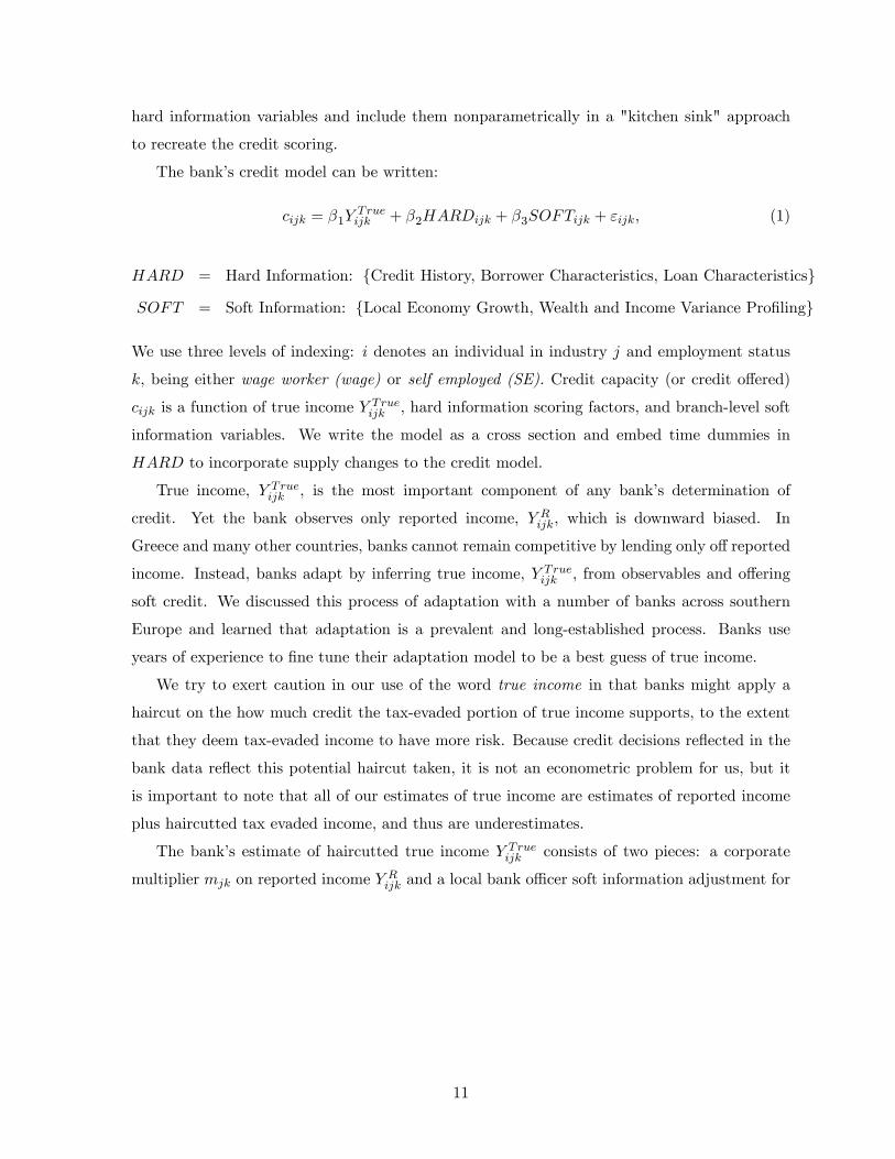
hard information variables and include them nonparametrically in a "kitchen sink" approach

to recreate the credit scoring.

The bank’s credit model can be written:

cijk = β1YTrueijk + β2HARDijk + β3SOFTijk + εijk, (1)

HARD = Hard Information: {Credit History, Borrower Characteristics, Loan Characteristics}

SOFT = Soft Information: {Local Economy Growth, Wealth and Income Variance Profiling}

We use three levels of indexing: i denotes an individual in industry j and employment status

k, being either wage worker (wage) or self employed (SE). Credit capacity (or credit offered)

cijk is a function of true income Y Trueijk , hard information scoring factors, and branch-level soft

information variables. We write the model as a cross section and embed time dummies in

HARD to incorporate supply changes to the credit model.

True income, Y Trueijk , is the most important component of any bank’s determination of

credit. Yet the bank observes only reported income, Y Rijk, which is downward biased. In

Greece and many other countries, banks cannot remain competitive by lending only off reported

income. Instead, banks adapt by inferring true income, Y Trueijk , from observables and offering

soft credit. We discussed this process of adaptation with a number of banks across southern

Europe and learned that adaptation is a prevalent and long-established process. Banks use

years of experience to fine tune their adaptation model to be a best guess of true income.

We try to exert caution in our use of the word true income in that banks might apply a

haircut on the how much credit the tax-evaded portion of true income supports, to the extent

that they deem tax-evaded income to have more risk. Because credit decisions reflected in the

bank data reflect this potential haircut taken, it is not an econometric problem for us, but it

is important to note that all of our estimates of true income are estimates of reported income

plus haircutted tax evaded income, and thus are underestimates.

The bank’s estimate of haircutted true income Y Trueijk consists of two pieces: a corporate

multiplier mjk on reported income Y Rijk and a local bank offi cer soft information adjustment for

11

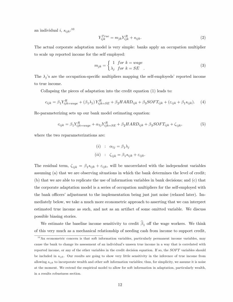
an individual i, sijk:10

Y Trueijk = mjkY

Rijk + sijk. (2)

The actual corporate adaptation model is very simple: banks apply an occupation multiplier

to scale up reported income for the self employed:

mjk =

{1 for k = wage

λj for k = SE .(3)

The λj’s are the occupation-specific multipliers mapping the self-employeds’reported income

to true income.

Collapsing the pieces of adaptation into the credit equation (1) leads to:

cijk = β1YRijk=wage + (β1λj)Y

Rijk=SE + β2HARDijk + β3SOFTijk + (εijk + β1sijk). (4)

Re-parameterizing sets up our bank model estimating equation:

cijk = β1YRijk=wage + α1jY

Rijk=SE + β2HARDijk + β3SOFTijk + ζijk, (5)

where the two reparameterizations are:

(i) : α1j = β1λj

(ii) : ζijk = β1sijk + εijk.

The residual term, ζijk = β1sijk + εijk, will be uncorrelated with the independent variables

assuming (a) that we are observing situations in which the bank determines the level of credit;

(b) that we are able to replicate the use of information variables in bank decisions; and (c) that

the corporate adaptation model is a series of occupation multipliers for the self-employed with

the bank offi cers’adjustment to the implementation being just just noise (relaxed later). Im-

mediately below, we take a much more econometric approach to asserting that we can interpret

estimated true income as such, and not as an artifact of some omitted variable. We discuss

possible biasing stories.

We estimate the baseline income sensitivity to credit β1 off the wage workers. We think

of this very much as a mechanical relationship of needing cash from income to support credit,

10An econometric concern is that soft information variables, particularly permanent income variables, may

cause the bank to change its assessment of an individual’s unseen true income in a way that is correlated with

reported income, or any of the other variables in the credit decision equation. If so, the SOFT variables should

be included in sijk. Our results are going to show very little sensitivity in the inference of true income from

allowing sijk to incorporate wealth and other soft information variables; thus, for simplicity, we assume it is noise

at the moment. We extend the empirical model to allow for soft information in adaptation, particularly wealth,

in a results robustness section.

12

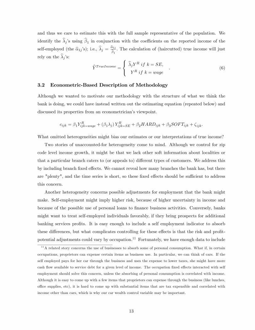
and thus we care to estimate this with the full sample representative of the population. We

identify the λj’s using β1 in conjunction with the coeffi cients on the reported income of the

self-employed (the α1j’s); i.e., λj =α1j

β1. The calculation of (haircutted) true income will just

rely on the λj’s:

Y TrueIncome =

λjYR if k = SE,

Y R if k = wage. (6)

3.2 Econometric-Based Description of Methodology

Although we wanted to motivate our methodology with the structure of what we think the

bank is doing, we could have instead written out the estimating equation (repeated below) and

discussed its properties from an econometrician’s viewpoint.

cijk = β1YRijk=wage + (β1λj)Y

Rijk=SE + β2HARDijk + β3SOFTijk + ζijk.

What omitted heterogeneities might bias our estimates or our interpretations of true income?

Two stories of unaccounted-for heterogeneity come to mind. Although we control for zip

code level income growth, it might be that we lack other soft information about localities or

that a particular branch caters to (or appeals to) different types of customers. We address this

by including branch fixed effects. We cannot reveal how many branches the bank has, but there

are "plenty", and the time series is short, so these fixed effects should be suffi cient to address

this concern.

Another heterogeneity concerns possible adjustments for employment that the bank might

make. Self-employment might imply higher risk, because of higher uncertainty in income and

because of the possible use of personal loans to finance business activities. Conversely, banks

might want to treat self-employed individuals favorably, if they bring prospects for additional

banking services profits. It is easy enough to include a self employment indicator to absorb

these differences, but what complicates controlling for these effects is that the risk and profit-

potential adjustments could vary by occupation.11 Fortunately, we have enough data to include

11A related story concerns the use of businesses to absorb some of personal consumption. What if, in certain

occupations, proprietors can expense certain items as business use. In particular, we can think of cars. If the

self employed pays for her car through the business and uses the expense to lower taxes, she might have more

cash flow available to service debt for a given level of income. The occupation fixed effects interacted with self

employment should solve this concern, unless the absorbing of personal consumption is correlated with income.

Although it is easy to come up with a few items that proprietors can expense through the business (like lunches,

offi ce supplies, etc), it is hard to come up with substantial items that are tax expensible and correlated with

income other than cars, which is why our car wealth control variable may be important.

13

self employment-crossed-with-occupation fixed effects. Combining, a more econometrically-

stringent model, with fixed effects abbreviated by f.e. is thus:

cijk = β1YRijk=wage + (β1λj)Y

Rijk=SE + β2HARDijk + β3SOFTijk

+f.e.Branch + f.e.Industry∗SE + ζijk.

This does not totally eliminate the possibility of an omitted variable, but the traits of such

a variable are a tall order. It would have to vary with income, unrelated to the local economy,

wealth, or income variability. The varying of this omitted variable with income would have to

be larger for the self-employed than for wage earners (to bias against us) and would have to

vary with occupation, differently than an overall adjustment of the self employment-occupation

fixed effects. We do not want to overclaim that it is certain that no such omitted (latent)

variable exists, but it is hard to make such an argument.

Another econometric point we want to discuss is the implication of wage workers tax evading.

To the extent that they do, our estimates of β1 will be too big. It will appear that a smaller

income supports more credit. Thus, our estimated of tax evasion will be conservative. Wage

workers might, however, tax evade differentially by income, implying that conservatism might

vary by industry. This means our ranking of which tax evaders are the biggest offenders might

not be correct. In addition, the possibility that the bank applies a haircut (in how much credit

tax evaded income supports) differentially by industry carries the same implication. When

we present results, we get comfortable using the terminology that some industries are ‘big’

tax evaders, rather than ‘biggest’tax evaders. However, this is an important issue to us, and

therefore we apply a host of validity tests to the industry rankings. In the end, hopefully we

are convincing that our ranking results are robust to allow us to interpret the findings.

4 Results

We begin by presenting results for each of the credit products. We then make inference by

precision-weighting the results from the individual products, a meta-analysis approach. By

using four very different loan products and different dependent variables, we capture not only

robustness across models but also information. As robustness, we then adjust the empirical

model to incorporate the inclusion of soft information in adaptation, using an approach that

provides bounds on the inference.

14

4.1 Constrained Sample Results

Table 3 reports the results for the constrained sample. The dependent variable is credit capacity,

defined to be total debt for individuals whose loan amount approved is lower than amount

requested and for individuals taking out an overdraft loan without large bank checking or

savings balances.12 Not included in the table presentation, but included in the estimation,

are all the covariates reported in column 1 of the appendix table, including borrower and loan

characteristics, borrower credit history, soft information variables, year dummies, and a self-

employment dummy.

The first row of Table 3 presents the coeffi cient (β1) on reported income for wage workers

(Y Rijk=wage). β1gives the baseline income sensitivity.

13 The remaining rows present the soft

credit coeffi cients on the self-employed reported income (Y Rijk=SE) by industry (the α1j’s). Recall

that we identify the income multiplier λ as λj =α1j

β1, which is what we present in the Lambda

columns following the coeffi cients. To give an example of interpretation, the first industry in

column 1 is Accounting and Financial Services. It has a self-employed coeffi cient on income

of 1.133 while the coeffi cient of income for wage workers is 0.520. This gives a lambda of just

above 2.

Going across the columns, the only difference in specifications is the inclusion of fixed

effects. Column 2 adds branch fixed effects, which only changes the results negligibly. Columns

3 adds industry crossed with self employment fixed effects, and column 4 adds both branch

and industry-self employment fixed effects. Although it is easy to be satisfied with the greater

econometric robustness that adding industry/self-employment fixed effects offers, it is not clear

that this robustness implies our estimates are better. The fixed effects for the self employed

industries are almost always negative, and the soft credit is larger (the λj’s are bigger). In

simple geometry, the line crosses the axis at less than zero with a steeper slope. We want to

exert caution in drawing magnitude inference solely from these larger coeffi cients.

Table 3 tells us that the bank applies the highest income multipliers to doctors, engineers

and scientists, lawyers, accountants, and financial service agents. In these industries, the self-

12Credit capacity itself is a combination of debt outstanding plus the credit capacity approved on the applied-

for loan. Since the new credit approved is the marginal addition to credit capacity, we assume that all credit

capacity (old loans plus new capacity) is equivalent in bank scoring. The ability of income to support debt

servicing is not particular to the origin or ordering of debt. We do analyses acrosss different credit models and

bank decisions to offer robustness to this and other assumptions.13As we mentioned earlier, the sensitivity of credit to income estimated off wage workers, should be lower than

the sensitivity estimate in Appendix TableA1 which includes both wage workers and tax-evading self-employed.

Indeed the sensitivity in table 3 is 0.52 in comparison to 0.635 for the constraint sample in Table A1.

15

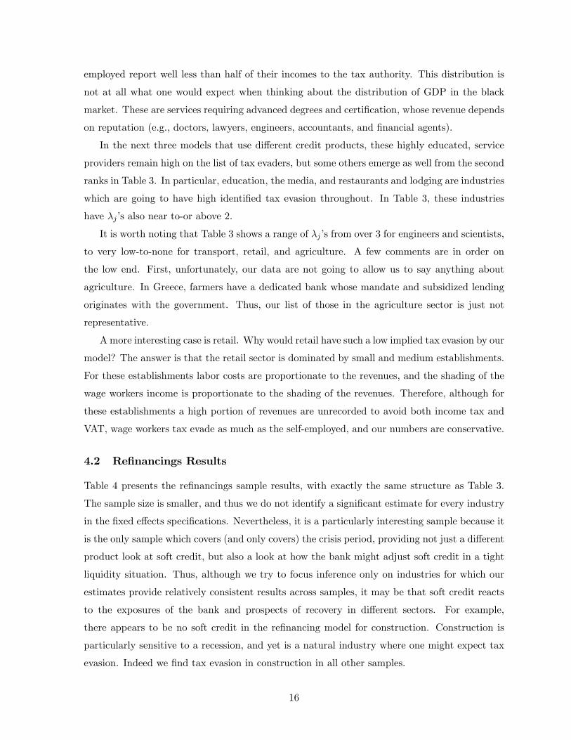
employed report well less than half of their incomes to the tax authority. This distribution is

not at all what one would expect when thinking about the distribution of GDP in the black

market. These are services requiring advanced degrees and certification, whose revenue depends

on reputation (e.g., doctors, lawyers, engineers, accountants, and financial agents).

In the next three models that use different credit products, these highly educated, service

providers remain high on the list of tax evaders, but some others emerge as well from the second

ranks in Table 3. In particular, education, the media, and restaurants and lodging are industries

which are going to have high identified tax evasion throughout. In Table 3, these industries

have λj’s also near to-or above 2.

It is worth noting that Table 3 shows a range of λj’s from over 3 for engineers and scientists,

to very low-to-none for transport, retail, and agriculture. A few comments are in order on

the low end. First, unfortunately, our data are not going to allow us to say anything about

agriculture. In Greece, farmers have a dedicated bank whose mandate and subsidized lending

originates with the government. Thus, our list of those in the agriculture sector is just not

representative.

A more interesting case is retail. Why would retail have such a low implied tax evasion by our

model? The answer is that the retail sector is dominated by small and medium establishments.

For these establishments labor costs are proportionate to the revenues, and the shading of the

wage workers income is proportionate to the shading of the revenues. Therefore, although for

these establishments a high portion of revenues are unrecorded to avoid both income tax and

VAT, wage workers tax evade as much as the self-employed, and our numbers are conservative.

4.2 Refinancings Results

Table 4 presents the refinancings sample results, with exactly the same structure as Table 3.

The sample size is smaller, and thus we do not identify a significant estimate for every industry

in the fixed effects specifications. Nevertheless, it is a particularly interesting sample because it

is the only sample which covers (and only covers) the crisis period, providing not just a different

product look at soft credit, but also a look at how the bank might adjust soft credit in a tight

liquidity situation. Thus, although we try to focus inference only on industries for which our

estimates provide relatively consistent results across samples, it may be that soft credit reacts

to the exposures of the bank and prospects of recovery in different sectors. For example,

there appears to be no soft credit in the refinancing model for construction. Construction is

particularly sensitive to a recession, and yet is a natural industry where one might expect tax

evasion. Indeed we find tax evasion in construction in all other samples.

16

The magnitude on the λj’s for accounting, finance, and medicine are slightly lower, but these

professions as well as lawyers and engineers remain robustly identified professions in which the

self-employed tax evade at least half of their income.

Education emerges as big tax-evading industry. To a non-Greek, this may seem odd. How-

ever, the system in Greece is such that anyone with a little excess disposable income hires

private tutors for their children. Not surprisingly, the private sector of tutoring is lucrative and

unrecorded. Media and art also emerge as high tax evaders. Journalists comprise the large

majority in the media related professions. Journalists in Greece have influence over political

decision making (they also have large presence in the parliament) and been enjoying lax regula-

tion regarding their income reporting. Art includes artists and actors. Both media and artists

have been among prominent cases of large tax evaders that the tax authorities have uncovered

during their recent controls.

4.3 Credit Card Limits Results

Table 5 reports the credit card sample results. The credit card sample is a quite different

model in the dependent variable is no longer credit capacity as a whole, but credit card limits,

controlling for debt outstanding. Thus, we are able to look for consistency in results for a

very different credit decision. Also important is that the credit cards sample will have some

individuals who are constrained, but the majority should be just individuals getting the new

payments product. In this sense, this model is the most population representative we have.

We find the big tax evaders to be in education, construction, law, and the media and art.

Accounting and financial services as well as medicine are slightly lower than in previous models,

but still identified. This may not be surprising since the credit card model is probably poorly

specified for high income individuals. Credit card limits become very concave (asymptote) at

the upper end of income. The largest credit card limit we have in the sample is 35,000 euros.14

4.4 Mortgage Payments Results

Finally, the last sample is the mortgage approved applicants of Table 6. The mortgage depen-

dent variable is the approved monthly payment implied by the mortgage amount, duration,

and interest rate. The mortgage estimation is the hardest to accomplish, because it is unclear

whether we should be estimating just an approval model or the mortgage details given approval.

The concern with estimating approvals is that dichotomous estimations offer very little of the

14We chose not to try to model this shape because were more interested in the bulk of Greeks who would be

on the linear part of the relationship between income and credit limits.

17

precision we are going to need to identify the industry distribution. The issue with estimating

the monthly payments amount is that the selection of who gets approved is severe.

Thus, we estimate a Heckman sample selection model (with additional first stage variables)

where we let the selection of approvals be estimated in the first stage, and mortgage payments

as the outcome equation.

Approvei = φ2HARDi + φ3SOFTi + µIndustry j + µSelfEmployed∗Industry j + ς i

MortgagePaymentsi = β1YRijk=wage + α1jY

Rijk=SE + β2HARDijk + α2SOFTijk +Millsi + ζijk

A pure Heckman selection model, which identifies off distributional assumptions only, is valid

under stringent assumptions which are hard to prove. Assumptions aside, we cannot identify

the model with so many dichotomous and interacted variables. Thus, we include additional

variables in the first stage. Because we need the selection estimation to remove industry bias,

in a conservative way, we specify the approval sample selection to depend on the industry fixed

effects and industry crossed with self-employment fixed effects. We also let the sample selection

depend on outstanding debt and the outcome payments model to depend on payments on prior

debt.15 Our goal in introducing the mortgage sample is modest. We want to show robustness of

our prior results to a different credit product with a different slice of the population. The vast

majority of Greeks own houses, and thus this common good of a mortgage gives us a perspective

on the population for those who are, generally, net savers.

Column 1 of Table 6 are the mortgage payment OLS estimates, without the application

approval correction. Columns 2 and 3 present the Heckman two stage results, with branch

fixed effects added in column 3. The results are surprisingly similar among the three columns,

but nevertheless, we stick to interpreting column 3.

We find that accountants, financial service professionals, doctors and engineers are the big

tax evaders implied by soft credit in mortgages. Lawyers have slightly lower tax evasion than

in prior estimations, but nevertheless identified. Note that mortgages are long-term exposure

by the bank. Thus, we feel these results are compelling.

4.5 Soft Information in Bank Adaptation

Recalling from above, the bank’s estimate of haircutted true income Y Trueijk consists of two

pieces: a corporate multiplier function mjk on reported income Y Rijk and a local bank offi cer

15We have just written the selection correction asMills to refer to the correlation-inverse Mills term estimated

in the first stage.

18

soft information adjustment for an individual i, sijk:

Y Trueijk = mjkY

Rijk + sijk,

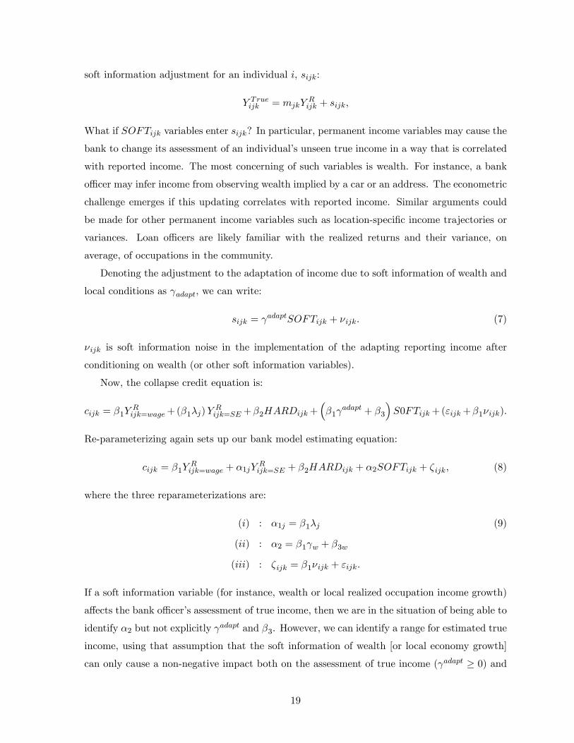
What if SOFTijk variables enter sijk? In particular, permanent income variables may cause the

bank to change its assessment of an individual’s unseen true income in a way that is correlated

with reported income. The most concerning of such variables is wealth. For instance, a bank

offi cer may infer income from observing wealth implied by a car or an address. The econometric

challenge emerges if this updating correlates with reported income. Similar arguments could

be made for other permanent income variables such as location-specific income trajectories or

variances. Loan offi cers are likely familiar with the realized returns and their variance, on

average, of occupations in the community.

Denoting the adjustment to the adaptation of income due to soft information of wealth and

local conditions as γadapt, we can write:

sijk = γadaptSOFTijk + νijk. (7)

νijk is soft information noise in the implementation of the adapting reporting income after

conditioning on wealth (or other soft information variables).

Now, the collapse credit equation is:

cijk = β1YRijk=wage + (β1λj)Y

Rijk=SE +β2HARDijk +

(β1γ

adapt + β3

)S0FTijk + (εijk +β1νijk).

Re-parameterizing again sets up our bank model estimating equation:

cijk = β1YRijk=wage + α1jY

Rijk=SE + β2HARDijk + α2SOFTijk + ζijk, (8)

where the three reparameterizations are:

(i) : α1j = β1λj (9)

(ii) : α2 = β1γw + β3w

(iii) : ζijk = β1νijk + εijk.

If a soft information variable (for instance, wealth or local realized occupation income growth)

affects the bank offi cer’s assessment of true income, then we are in the situation of being able to

identify α2 but not explicitly γadapt and β3. However, we can identify a range for estimated true

income, using that assumption that the soft information of wealth [or local economy growth]

can only cause a non-negative impact both on the assessment of true income (γadapt ≥ 0) and

19

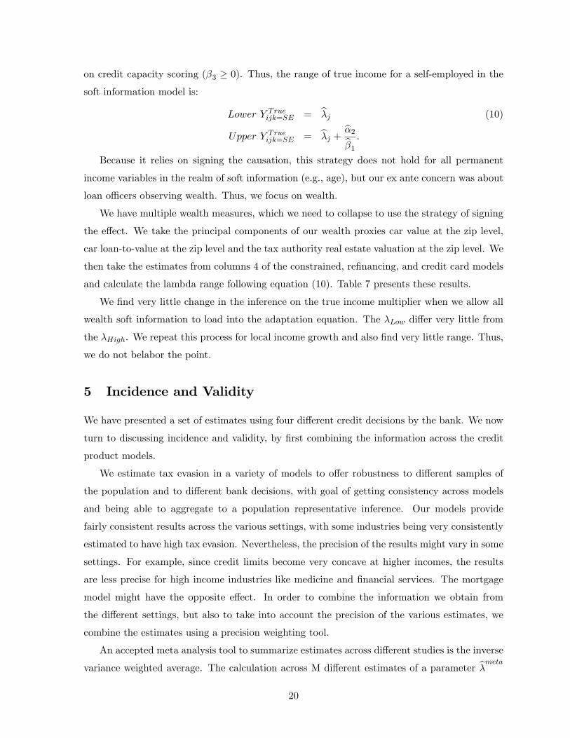
on credit capacity scoring (β3 ≥ 0). Thus, the range of true income for a self-employed in the

soft information model is:

Lower Y Trueijk=SE = λj (10)

Upper Y Trueijk=SE = λj +

α2

β1.

Because it relies on signing the causation, this strategy does not hold for all permanent

income variables in the realm of soft information (e.g., age), but our ex ante concern was about

loan offi cers observing wealth. Thus, we focus on wealth.

We have multiple wealth measures, which we need to collapse to use the strategy of signing

the effect. We take the principal components of our wealth proxies car value at the zip level,

car loan-to-value at the zip level and the tax authority real estate valuation at the zip level. We

then take the estimates from columns 4 of the constrained, refinancing, and credit card models

and calculate the lambda range following equation (10). Table 7 presents these results.

We find very little change in the inference on the true income multiplier when we allow all

wealth soft information to load into the adaptation equation. The λLow differ very little from

the λHigh. We repeat this process for local income growth and also find very little range. Thus,

we do not belabor the point.

5 Incidence and Validity

We have presented a set of estimates using four different credit decisions by the bank. We now

turn to discussing incidence and validity, by first combining the information across the credit

product models.

We estimate tax evasion in a variety of models to offer robustness to different samples of

the population and to different bank decisions, with goal of getting consistency across models

and being able to aggregate to a population representative inference. Our models provide

fairly consistent results across the various settings, with some industries being very consistently

estimated to have high tax evasion. Nevertheless, the precision of the results might vary in some

settings. For example, since credit limits become very concave at higher incomes, the results

are less precise for high income industries like medicine and financial services. The mortgage

model might have the opposite effect. In order to combine the information we obtain from

the different settings, but also to take into account the precision of the various estimates, we

combine the estimates using a precision weighting tool.

An accepted meta analysis tool to summarize estimates across different studies is the inverse

variance weighted average. The calculation across M different estimates of a parameter λmeta

20

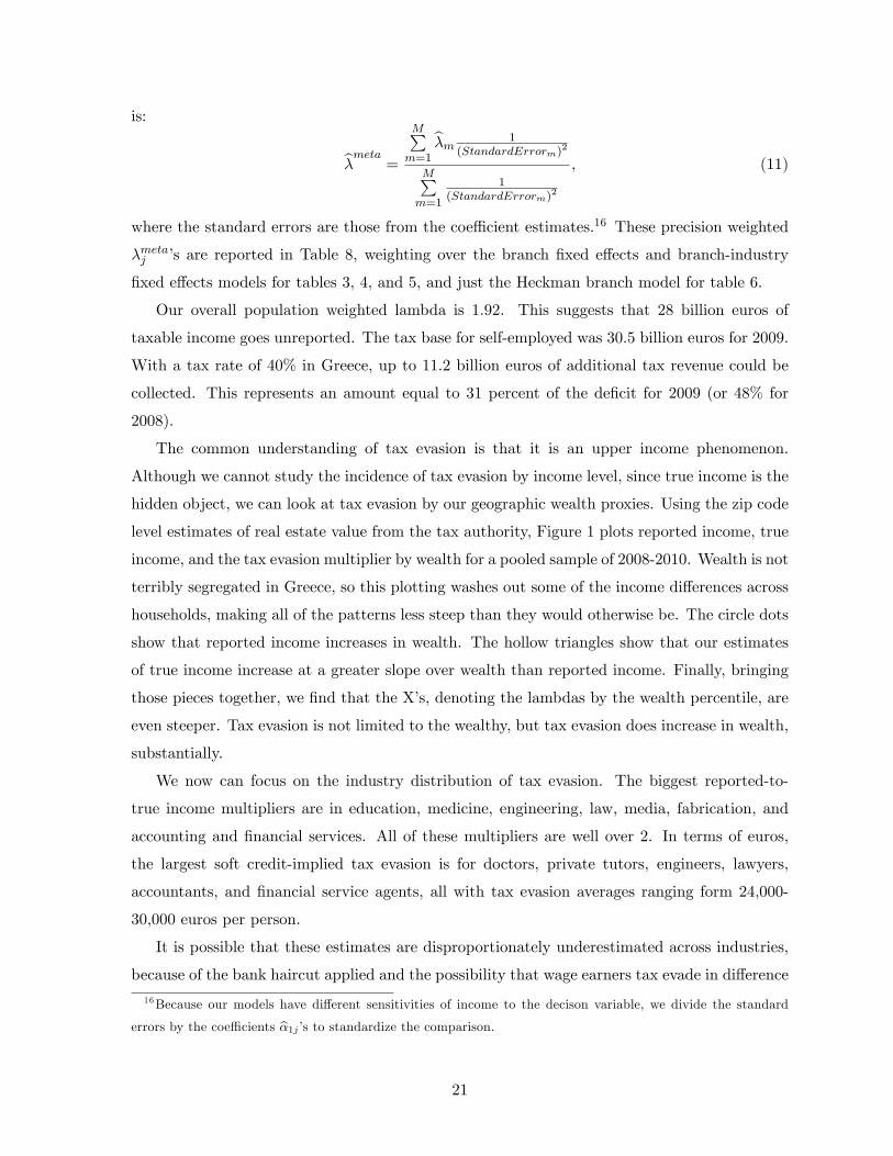
is:

λmeta

=

M∑m=1

λm1

(StandardErrorm)2

M∑m=1

1(StandardErrorm)

2

, (11)

where the standard errors are those from the coeffi cient estimates.16 These precision weighted

λmetaj ’s are reported in Table 8, weighting over the branch fixed effects and branch-industry

fixed effects models for tables 3, 4, and 5, and just the Heckman branch model for table 6.

Our overall population weighted lambda is 1.92. This suggests that 28 billion euros of

taxable income goes unreported. The tax base for self-employed was 30.5 billion euros for 2009.

With a tax rate of 40% in Greece, up to 11.2 billion euros of additional tax revenue could be

collected. This represents an amount equal to 31 percent of the deficit for 2009 (or 48% for

2008).

The common understanding of tax evasion is that it is an upper income phenomenon.

Although we cannot study the incidence of tax evasion by income level, since true income is the

hidden object, we can look at tax evasion by our geographic wealth proxies. Using the zip code

level estimates of real estate value from the tax authority, Figure 1 plots reported income, true

income, and the tax evasion multiplier by wealth for a pooled sample of 2008-2010. Wealth is not

terribly segregated in Greece, so this plotting washes out some of the income differences across

households, making all of the patterns less steep than they would otherwise be. The circle dots

show that reported income increases in wealth. The hollow triangles show that our estimates

of true income increase at a greater slope over wealth than reported income. Finally, bringing

those pieces together, we find that the X’s, denoting the lambdas by the wealth percentile, are

even steeper. Tax evasion is not limited to the wealthy, but tax evasion does increase in wealth,

substantially.

We now can focus on the industry distribution of tax evasion. The biggest reported-to-

true income multipliers are in education, medicine, engineering, law, media, fabrication, and

accounting and financial services. All of these multipliers are well over 2. In terms of euros,

the largest soft credit-implied tax evasion is for doctors, private tutors, engineers, lawyers,

accountants, and financial service agents, all with tax evasion averages ranging form 24,000-

30,000 euros per person.

It is possible that these estimates are disproportionately underestimated across industries,

because of the bank haircut applied and the possibility that wage earners tax evade in difference

16Because our models have different sensitivities of income to the decison variable, we divide the standard

errors by the coeffi cients α1j’s to standardize the comparison.

21

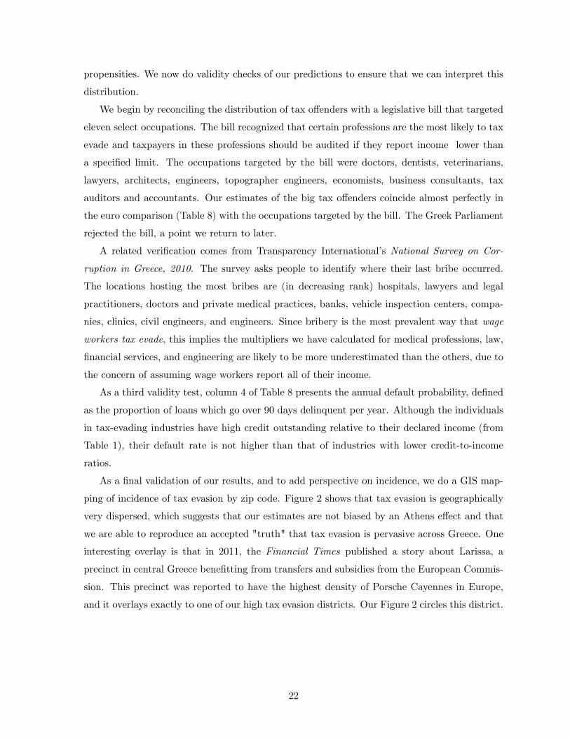
propensities. We now do validity checks of our predictions to ensure that we can interpret this

distribution.

We begin by reconciling the distribution of tax offenders with a legislative bill that targeted

eleven select occupations. The bill recognized that certain professions are the most likely to tax

evade and taxpayers in these professions should be audited if they report income lower than

a specified limit. The occupations targeted by the bill were doctors, dentists, veterinarians,

lawyers, architects, engineers, topographer engineers, economists, business consultants, tax

auditors and accountants. Our estimates of the big tax offenders coincide almost perfectly in

the euro comparison (Table 8) with the occupations targeted by the bill. The Greek Parliament

rejected the bill, a point we return to later.

A related verification comes from Transparency International’s National Survey on Cor-

ruption in Greece, 2010. The survey asks people to identify where their last bribe occurred.

The locations hosting the most bribes are (in decreasing rank) hospitals, lawyers and legal

practitioners, doctors and private medical practices, banks, vehicle inspection centers, compa-

nies, clinics, civil engineers, and engineers. Since bribery is the most prevalent way that wage

workers tax evade, this implies the multipliers we have calculated for medical professions, law,

financial services, and engineering are likely to be more underestimated than the others, due to

the concern of assuming wage workers report all of their income.

As a third validity test, column 4 of Table 8 presents the annual default probability, defined

as the proportion of loans which go over 90 days delinquent per year. Although the individuals

in tax-evading industries have high credit outstanding relative to their declared income (from

Table 1), their default rate is not higher than that of industries with lower credit-to-income

ratios.

As a final validation of our results, and to add perspective on incidence, we do a GIS map-

ping of incidence of tax evasion by zip code. Figure 2 shows that tax evasion is geographically

very dispersed, which suggests that our estimates are not biased by an Athens effect and that

we are able to reproduce an accepted "truth" that tax evasion is pervasive across Greece. One

interesting overlay is that in 2011, the Financial Times published a story about Larissa, a

precinct in central Greece benefitting from transfers and subsidies from the European Commis-

sion. This precinct was reported to have the highest density of Porsche Cayennes in Europe,

and it overlays exactly to one of our high tax evasion districts. Our Figure 2 circles this district.

22

6 Making Sense of the Industry Distribution

In this section, we discuss out how theory might approach explaining the distribution of in-

dustries or occupations and then put forth evidence for consistency. Admittedly, we do not

know whether the causes of the industry distribution in Greece would be the dominant ones in

other countries, but this in no way hinders our being able to speak to the potential for different

theories to matter.

We begin with theories as to when and where allowing tax evasion might be optimal for

the economy. We will find no support for these ideas and quickly move to stories of incentives

helping to support the distribution.

(i) Intent of the Government Stories:Subsidizing Risk Taking or Apprentice Training

Pestieau and Possen (1991) argue that governments might overlook tax evasion by entre-

preneurs in order to subsidize risk taking in the economy. The picture of growth entrepreneurs

at startup is not, however, the picture of the self-employment landscape in Greece, which looks

more like what Hurst and Pugsley, (2011) document, namely, professional and personal ser-

vice practices and mom-and-pops’. In addition, the largest tax-evading professions are ones

for which education removes income uncertainty (doctors, lawyers), consistent with the lack of

risk-subsidizing effects in occupational choice of Parker (1999).17

Nevertheless, it is true that scientists and engineers are tax offenders in our distribution and

perhaps the spirit of the theory would suggest that government might overlook tax evasion more

where growth multiplies into the local economy. To investigate this theory (and a subsequent

enforcement incentive theory), we gather detailed enforcement records from the tax authority

of Greece. The Greek tax authority started to publish statistics in January 2011 in response to

the public outcry against the low effi ciency of tax collection. We have daily data for each of 235

tax authority offi ces in three metrics: the number of cases the offi ce is assigned (automatically

by the central system), the number of cases the offi ce closes on a given day, and the amount

assessed to the taxpayer with these closes. Our metrics of interest are the sum of cases closed

for the year per taxfiler and the sum of the amount assessed per closed case. We control for

the number of cases assigned per taxfiler by the central system.

To see whether the tax authority avoids prosecuting tax offenders in high local growth areas,

we map the 1,569 zip codes to the 235 tax offi ces and run a simple regression of 2011 enforce-

ments, in particular, the log of cases closed and the log of assessments per close, iteratively, on

17The proposition that insuffi cient numbers of doctors and lawyers exist in Greece would be rejected by most

Greeks.

23

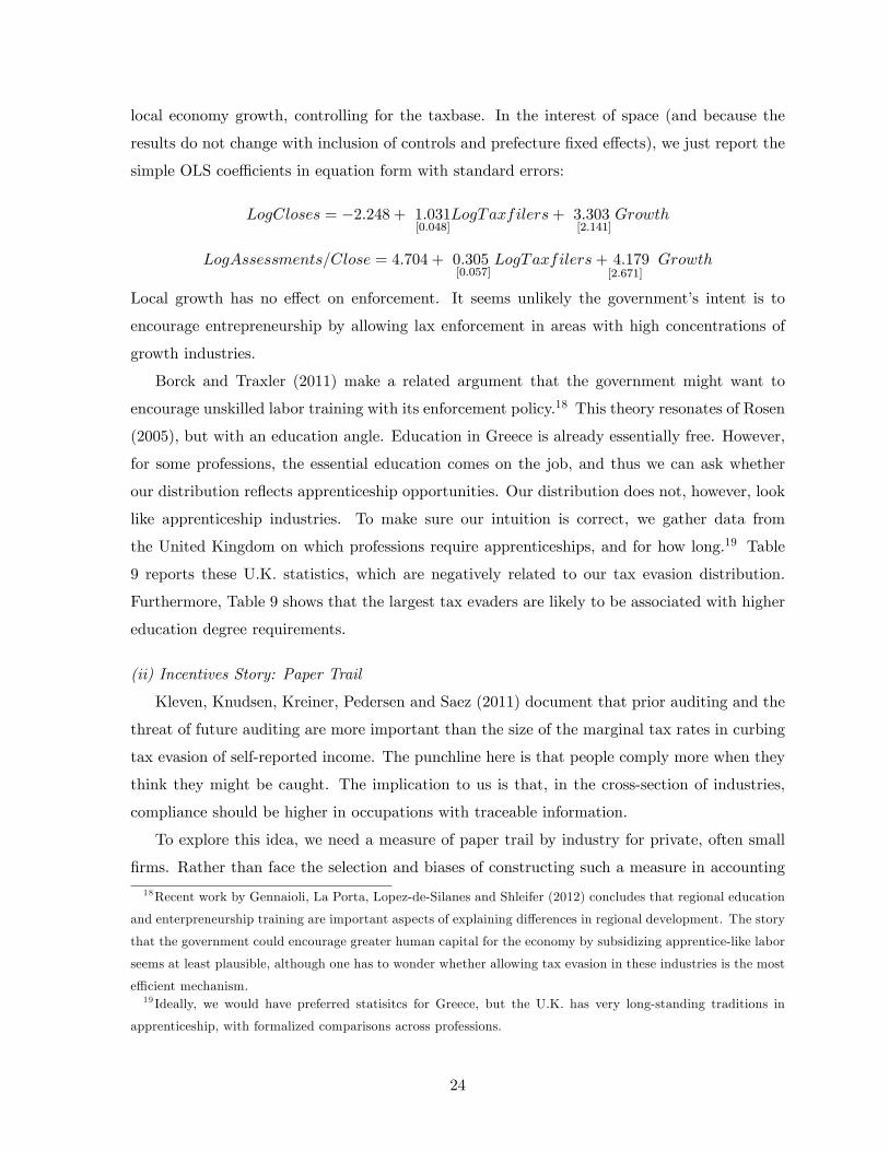
local economy growth, controlling for the taxbase. In the interest of space (and because the

results do not change with inclusion of controls and prefecture fixed effects), we just report the

simple OLS coeffi cients in equation form with standard errors:

LogCloses = −2.248 + 1.031[0.048]

LogTaxfilers+ 3.303[2.141]

Growth

LogAssessments/Close = 4.704 + 0.305[0.057]

LogTaxfilers+ 4.179[2.671]

Growth

Local growth has no effect on enforcement. It seems unlikely the government’s intent is to

encourage entrepreneurship by allowing lax enforcement in areas with high concentrations of

growth industries.

Borck and Traxler (2011) make a related argument that the government might want to

encourage unskilled labor training with its enforcement policy.18 This theory resonates of Rosen

(2005), but with an education angle. Education in Greece is already essentially free. However,

for some professions, the essential education comes on the job, and thus we can ask whether

our distribution reflects apprenticeship opportunities. Our distribution does not, however, look

like apprenticeship industries. To make sure our intuition is correct, we gather data from

the United Kingdom on which professions require apprenticeships, and for how long.19 Table

9 reports these U.K. statistics, which are negatively related to our tax evasion distribution.

Furthermore, Table 9 shows that the largest tax evaders are likely to be associated with higher

education degree requirements.

(ii) Incentives Story: Paper Trail

Kleven, Knudsen, Kreiner, Pedersen and Saez (2011) document that prior auditing and the

threat of future auditing are more important than the size of the marginal tax rates in curbing

tax evasion of self-reported income. The punchline here is that people comply more when they

think they might be caught. The implication to us is that, in the cross-section of industries,

compliance should be higher in occupations with traceable information.

To explore this idea, we need a measure of paper trail by industry for private, often small

firms. Rather than face the selection and biases of constructing such a measure in accounting

18Recent work by Gennaioli, La Porta, Lopez-de-Silanes and Shleifer (2012) concludes that regional education

and enterpreneurship training are important aspects of explaining differences in regional development. The story

that the government could encourage greater human capital for the economy by subsidizing apprentice-like labor

seems at least plausible, although one has to wonder whether allowing tax evasion in these industries is the most

effi cient mechanism.19 Ideally, we would have preferred statisitcs for Greece, but the U.K. has very long-standing traditions in

apprenticeship, with formalized comparisons across professions.

24

data, we apply a survey instrument. We surveyed a class of 25 executives in an executive

business program in Greece.20 We chose business executives who selected to be in a masters

program because such individuals would be experienced in inflows and outflows of industries

and the accounting thereof.

The participants were asked to score each industry on a scale of 1-5 on (i) the use of

intermediate goods as inputs and (ii) the extent to which the output is an intermediate good.

For tax evasion purposes, input paper trail may be as important as output paper trail. Doctors

and pharmacists may both sell to end users who require no paper trail, but pharmacists may

have to account for their inputs. We de-mean each individual’s responses to capture any level

biases by individuals. Table 9 presents the mean scores of paper trail input and output by

industry.

We find that industries with high paper trail are less likely to be tax evaders. The correla-

tions, at the bottom of the table, are between -0.25 to -0.30, both on input and output measure

of paper trail.

Perhaps the more poignant take-aways from the table are in the intuition for specific in-

dustries. Industries with high paper trail as an input are construction, fabrication, restaurants,

and retail. These are not the highest tax evaders. Industries with the lowest input paper trail

include some of our biggest tax evaders —law, education, and accounting and financial services.

Turning to the output measures of paper trail, industries with high scores are construction,

engineering, transport, and fabrication. Included in industries with low output paper trail are

doctors, education, accounting and financial services, all high tax evaders. Journalists and

artists (in industry Media & Art) are occupations low on input and output paper trail, for

which we find fairly high tax evasion.

Although we cannot assert causation in this simple correlation exercise, we find this evidence

intuitive and convincing. One need not look to our survey to imagine that pharmacy and

transport have a high paper trail, whereas services like doctors and private tutors do not. Our

belief is that the lack of a paper trail is indeed a primary driver of the industry distribution of

tax evasion.

(iii) Incentive Story: Enforcement Willpower

For enforcement offi cials, the flip side being able to see paper trail of tax evasion is having

the willpower to do the enforcement. Perhaps enforcement by tax auditors is skewed toward

certain industries. To investigate enforcement willpower across industries, ideally, we would

20We conducted the survey at the University of Piraeus in an executives program in a financial economics

class. Participation was 25 out of 30.

25

overlay enforcement statistics with industry distributions at the 235 tax offi ce districts, but our

sample is just not suffi ciently large to be representative of industries at that level. However, we

can study enforcements incentives, as they relate to self-employment and wealth. The thought

experiment is that since our largest tax evading occupations are also high-wealth occupations

(see Table 1), we can ask whether tax offi cials enforce tax evasion more in areas with high

wealth and high numbers of self-employed. We know the percent of taxfilers in the zip code

who are self-employed (categorized either as merchants or other self-employed in the tax data)

as well as wealth, as measured by the tax authority real estate estimate. We collapse these zip

code statistics to the districts of 235 tax enforcement offi ces and merge with the enforcement

data described earlier in this section. Panel A of Table 10 reports the summary statistics of

these data.

Panel B presents the analysis, starting with the number of closes as the dependent variable.

Closes is right skewed, so we do the analysis of columns 1 as elasticities (in logs) and then as

a poisson (columns 4-6). Columns 1 and 4 show the elasticity, and poisson rate sensitivity, of

cases closed to self-employment percent is strongly positive and significant. Closes are more

weakly, positively related to wealth. In columns 2 and 5, we add the interesting interaction

of wealth and self-employment. However, we do not put much weight on these columns, as

wealth and self-employment are very correlated with the interaction, with variance inflation

factors (VIFs) being over 200. Thus, we orthogonalize the variables using the modified Gram-

Schmidt procedure of Golub and Van Loan (1996), which gives the most importance weight

to the level variables and let the interaction only capture what is left over. The interaction of

wealth and self-employment is positive and significant. The percent of self-employed remains

significant. Local tax offi cials are more able to closing cases generally in places high numbers

of self- employed, but especially in places with wealthy self-employed. This result, which is

encouraging for the efforts of the tax authorities, does not help us to explain the distribution

of tax evasion. It appears that tax authorities are going after those most evading.

However, when we repeat the exercise for the assessment amount, our results are mixed.

The first dependent variable in columns 7-9 is (the log of) the intuitive variable of assessments

(in Euro) per close. Furthermore, in columns 10-12, we make sure results are not determined

by the denominator by using just log assessments as the dependent variable, moving closes to

the right hand side. We do the same exercise with orthogonalization. We find that the percent

self-employed is significant throughout, but wealth has no role at all.

The fact that the tax offi cers close more cases in wealthy areas and areas with high per-

centage of self-employed suggests that the rich and especially the rich self-employed are not

26

under the radar of the tax authorities. Thus, it does not seem that intimidation from the rich

and powerful of the form suggested by Glaeser, Scheikman and Shleifer (2003) is at work here.

However, the result that assessments have no relation to wealth, while closes do, is unfortu-

nately consistent with the 4-4-2 system of side payments, exposed in the New York Times.

In December 2011, the head of the Greek Anti-Tax Evasion Unit, publicly described the 4-

4-2 system in which the default rule between Greek tax collectors and tax evaders is that 40

percent of a taxpayer’s assessment of evasion would be forgiven; 40 percent would be paid to

the tax agent; and the remaining 20 percent would be paid to the state.21 The fact that the

closes are happening but assessments are not increasing with wealth for the self-employed is

very consistent with agents following their incentives and wealthy understanding that the side

payment system ‘works’in the sense of Shleifer and Vishny (1993). We do not want to be too

negative on the tax authority from this exercise. We were encouraged that the relation between

self-employment and closes was so strong. Clearly, the tax authority has internal knowledge

and is not ignoring the high tax evading industries, but changes have to be introduced in the

incentive structure.

Although this analysis of enforcement incentives and effectiveness is certainly interesting,

the evidence does not support the idea that enforcement willpower across occupations explains

our distribution. In fact, it is contradictory. Tax collectors appear to go after those in wealthier

self-employment professions. The wealthier professions are among our biggest tax evaders —

doctors, lawyers, engineers, and fabrication.

(iv) Incentive Story: Political Willpower

The final story to understand the industry distribution of tax evasion reflects back to the

legislative bill, which did not pass, that would have targeted for tax audits individuals with

income below a presumed income for select industries. The bill called for targeted tax audits for

declared income bellow 20,000 euros on the likes of doctors, lawyers, and engineers, including

most of our high tax-offending industries. The quick dismissing of this bill motivated us to ask

whether the distribution of tax evading industries be related to politicians looking out for their

own profession or, said another way, to the power of industry associations and guilds?22 Ideally,

21New York Times, February 2, 2012.22We looked for academic work to support our hypothesis that politicians may look after their former (and

possibily future) occupations, because of the benefits of personal networks, loyalty, or future income prospects.

Although there is a very large literature on interest groups and lobbist selection of politicians, there seems to

be little work supporting this hypothesis, perhaps because of the prevalence of lawyers in the political arena in

many countries. Faccio (2006) offers evidence that politicians support their family industries, which may also be

the current politician’s occupation.

27

we would like to see the distribution of votes on that bill, but Greek votes are not made public.

Instead, we look up the occupational backgrounds of the 2009 Greek parliamentarians to see

whether they correlate with tax evading professions. We download the names and biographies

from the Parliament website. Most curriculum vita appear on Parliament website or personal

webpages. For the others, we look up their histories, easily, on the internet since these people

are in the public domain.

Table 12 presents the results, ordered in a descending sort of tax evading industries. We

want to draw attention to the cumulative distribution of parliamentary members (the fifth

column), tossing out lawyers as the default profession for politicians. The idea is to see how

quickly or slowly the tax evading professions add up to the getting a voting majority or super-

majority. Out of fourteen industries, the three most tax-evading account for about half (0.483)

of the Parliamentary votes; the four most tax-evading industries account for approximately a

supermajority (0.657) of votes.

We know that we cannot claim causality from this table that politicians do not have

willpower to enforce tax evasion.23 Nevertheless, we can take this suggestive picture one step

further and compare the distribution of politicians to a benchmark. We chose to do so against

Canada. Canada is appealing in being a country with high levels of public services, a very

sophisticated banking sector, a parliamentary government, and a very low level of tax evasion.

Admittedly, we chose Canada over other candidates with these Greek-like attributes other than

tax evasion (e.g., Scandinavia) because of the ability to find the biographies of the parliamen-

tarians (in English). The Canadian Parliament posts links to websites and curriculum vitaes

for each member, from which we code occupations for each of the 304 Parliamentarians.

Table 12 shows that the occupational distribution of 2011 Parliamentarians for Canada

loads much less on tax-evading professions. The first three industries (sorted by declining tax

evasion) only account for 27% of Parliament votes for Canada. This was nearly half of the votes

for Greece. Likewise, a supermajority of votes for Canada is not reached until the 9th out of

14 occupations are added to the list.

Although we cannot claim that the roots of the industry distribution of tax evasion is politi-

cal, surely it is not a stretch to say that the combination of the rejection of the minimum income

23Having said that, others do make this claim. The New York Times, February 2, 2012, reports:

“In Greece, the real power is the power of resistance, the power of inertia,” said Giorgos Floridis, a former

member of Parliament from the Socialist Party who recently founded a reform-minded civic movement. Today,

he said, the main power centers in Greece – political parties, business leaders, professional guilds, public sector

unions and the media – are fighting to preserve their privileges, blocking structural changes that could make

the economy more functional."

28

tax bill of 2010 and their occupational distribution certifies their current lack of willpower on

this issue.

Summary of Industry Distribution Findings

In summary, our industry distribution of tax evaders in Greece provides support for two

incentive stories of tax evasion. Our distribution of tax evasion is very consistent with the idea

that paper trail matters. Industries with lower intensity of paper trail have more tax evasion,

both in their reported income multiplier and in euros hidden. In addition, we find a very

surprisingly strong correlation between Parliamentary members and the ranking of tax evasion

industries. We do a simple benchmark test against Canada, showing that indeed Greece’s

Parliament is very skewed toward tax evading industry associations.

7 Conclusion

Harberger (2006) introduces the idea that the private sector adapts to norms of tax evasion.

We borrow that idea, show that banks adapt their lending to semiformal income, and develop a

new methodology to estimate tax evasion. Using individual-level household lending data across

four credit products, we estimate that 28 billion euros in self-employed income goes untaxed in

Greece for 2009, accounting for 31 percent of the deficit for 2009 or 48% for 2008.

Ranked by euros tax-evaded, the largest offending industries are medicine, engineering,

education, accounting and financial services, and law. This industry distribution of tax evaders

in Greece provides support for two incentive stories. First, paper trail matters. Industries

with lower intensity of paper trail have more tax evasion. Second, politicians matter. The

occupations of parliamentarians line up very well with the tax evading occupations, and these

same parliamentarians failed to pass mild reform targeting their own industries.

An observation from our study might be of interest to policymakers. Presumed income tax

initiatives, under which the government mandates a minimum tax reporting by occupation,

are politically unsavory. However, one observation from our results is that the distribution of

professions tax evading are establishments. Thus, policy professionals might consider whether

occupation licenses for tax evading industries might line up with our rankings. City authorities

world-wide use business licenses to collect revenues, and in the case of Greece, the list of

professions tax evading is strongly related to the existence of mandatory industry associations,

providing a potential forum for collections.

A final thought concerns the welfare implications of bank issuing of soft credit. Although we

are limited in space and data to accomplish a study of welfare, we would like to introduce ideas

29

since the observation of bank adaptation to semiformality is new. In a Coasian or De Soto view

of the world, the fact that banks give an entitlement to informal income provides a property

right that allows individuals to use borrowing to optimally smooth lifetime consumption or

overcome shocks. A negative side is that access to soft credit reduces the costs to informality,

but we would be surprised if the negative outweighs the positive in the second best world of a

norm of semiformality.

This welfare discussion raises (at least) three points. It would be interesting to study

commercial lending under this frame. It would also be interesting to know the extent to the

haircut imposed on tax evaded income and to speak to the welfare benefit accruing to borrowers.

Finally, the idea that informal income is a property right with entitlement benefits like a farm

deed is new and interesting. To our knowledge, soft information has not been documented to

increase the size of the lending pie previously, although it most certainly does, in contexts other

than soft credit.

30

8 References

Adams, William, Liran Einav and Jonathan Levin, 2009.“Liquidity Constraints and Imperfect

Information in Subprime Lending.”American Economic Review, Vol. 99(1), pp. 49-84.

Allingham, Michael G. and Agnar Sandmo, 1972. "Income Tax Evasion: A Theoretical Analy-

sis." Journal of Public Economics, Vol. 1, pp. 323-338.

Antunes Antonio R. and Tiago V. de V. Cavalcanti, 2007. "Start up Costs, Limited Enforce-

ment, and the Hidden Economy." European Economic Review, Vol. 51 (1), pp. 203-224.

Andreoni, James, Brian Erard, and Jonathan Feinstein, 1998. "Tax Compliance." Journal of

Economic Literature, Vol. XXXVI, pp. 818-60.

Banerjee, Abhijit, and Esther Duflo, 2005. “Growth Theory through the Lens of Development

Economics,” in Handbook of Economic Growth, Vol. 1A, P. Aghion and S. Durlauf, eds.

Amsterdam: Elsevier.

Braguinsky, Serguey , Sergey Mityakov, and Andrey Liscovich, 2010. "Direct Estimation of

Hidden Earnings: Evidence From Administrative Data." Working Paper.

Cagan, Phillip, 1958. "The Demand for Currency Relative to the Total Money Supply." Journal

of Political Economy, Vol. 66(4), pp. 303-28.

Chetty, Raj and Emmanuel Saez, 2010. "Optimal Taxation and Social Insurance with En-

dogenous Private Insurance." American Economic Journal: Economic Policy, Vol. 2(2), pp.

85-114.

Christian, Charles, 1994. "Voluntary Compliance with the Individual Income Tax: Results

from the 1988 TCMP study". IRS Research Bulletin, Publication 1500, pp. 35—42.

Faccio, Mara, 2006. "Politically Connected Firms." American Economic Review. Vol. 96(1),

pp. 369-386.

Feld, Lars P. and Friedrich Schneider, 2010. "Survey on the Shadow Economy and Undeclared

Earnings in OECD Countries." German Economic Review, Vol. 11 (2), pp. 109-149.

Feldman, Naomi E., and Joel Slemrod, 2007. "Estimating Tax Noncompliance with Evidence

from Unaudited Tax Returns." Economic Journal, Vol. 117(51), pp. 327-352.

31

Feinstein, Jonathan S., 1999. “Approaches for Estimating Noncompliance: Examples from

Federal Taxation in the United States.”Economic Journal, Vol. 109, pp. F360-F369.

Gennaioli, Nicola, Rafael La Porta, Florencia Lopez-de-Silanes and Andrei Shleifer, 2012. "Hu-

man Capital and Regional Development." Working Paper.

Glaeser, Edward, Jose Scheinkman, and Andrei Shleifer, 2003. "The Injustice of Inequality."

Journal of Monetary Economics, Vol. 50(1), pp. 199-222.

Gong, Xiadong and Arthus van Soest, 2002. "Wage Differentials and Mobility in the Urban

Labour Market: a Panel data analysis for Mexico." Labour Economics, Vol. 9, pp. 513-529.

Gorodnichenko, Yuri, Jorge Martinez-Vazquez, and Klara Sabirianova, 2009. “Myth and Re-

ality of Flat Tax Reform: Micro Estimates of Tax Evasion Response and Welfare Effects in

Russia.”Journal of Political Economy, Vol. 117 (3), 504-554.

Harberger, Arnold, 2006. "Reflections on Corruption: An Economist’s Perspective," U.S.

Agency for International Development Series: Strategic Objective or Activity: pp. 905-101.

Hurst, Erik, Geng Li Geng and Benjamin Pugsley, 2011. "Are Households Surveys Like Tax

Forms: Evidence from Income Underreporting of the Self Employed", Working Paper, Finance

and Economics Discussion Series, Board of Governonrs of the Federal Reserve System.

Hurst, Erik and Benjamin Pugsley, 2011."What Do Small Businesses Do?" Brookings Papers

on Economic Activity, Fall Volume.

Klepper, Steven and Daniel Nagin, 1989. "The anatomy of tax evasion." Journal of Law,

Economics, and Organization, Vol. 5(1), pp. 1—24.

Kleven, Henrik J., Martin B. Knudsen, Claus T. Kreiner, Soren Pedersen and Emmanuel Saez,

2011. "Unwilling or Unable to Cheat? Evidence from a Tax Audit Experiment in Denmark."

Econometrica, Vol. 79, pp. 651-692.

Lacko, Maria, 2000. "Hidden Economy - an Unknown Quantity? Comparative Analysis of

Hidden Economies in Transition Countries, 1989-95." Economics of Transition, Vol. 8(1), pp.

117-49.

Lyssiotou, Panayiota, Panos Pashardes, and Thanasis Stengos, 2004. "Estimates of the Black

Economy Based on Consumer Demand Approaches". Economic Journal, Vol. 114(497), pp.

622—40.

32

Pestieau, Pierre and Uri M. Possen, 1991. "Tax Evasion and Occupational Choice." Journal of

Public Economics, Vol. 45, pp. 307-325.

Parker, Simon C, 1999. "The Optimal Linear Taxation of Employment and Self-Employment

Incomes." Journal of Public Economics, Vol. 73, 107-123.

Pencavel, John H., 1979. "A Note on Income Tax Evasion, labor Supply, and Nonlinear Tax

Schedules." Journal of Public Economics, Vol. 12., pp. 115-124.

Pissarides, Christopher A. and Guglielmo Weber, 1989. "An Expenditure-Based Estimate of

Britian’s Black Economy." Journal of Public Economics, Vol. 39(1), pp. 17-32.

Rosen, Harvey S., 2005. Public Finance. New York: McGraw-Hill

Schneider, Friedrich and Dominik H. Enste, 2000. "Shadow Economies: Size, Causes and

Consequences." Journal of Economic Literature, Vol. 38(1), pp. 77-114.

Shleifer, Andrei and Robert Vishny, 1993. “Corruption.”Quarterly Journal of Economics, Vol.

108 (3), pp. 599-617.

Slemrod, Joel and Shlomo Yitzhaki, 1996. "The Costs of Taxation and the Marginal Effi ciency

Cost of Funds." IMF Staff Papers, Vol. 43(1), pp. 172-98.

Stiglitz, Joseph E. and Andrew Weiss, 1981. "Credit Rationing in Markets with Imperfect

Information." American Economic Review, Vol. 71 (3), pp. 393-410.

Tanzi, Vito, 1983. "The Underground Economy in the United States: Annual Estimates 1930-

1980". International Monetary Fund Stuff Papers, Vol. 30, pp. 283-305.

33

34  

Figure 1: Tax Evasion by Wealth Using the tax authority real estate valuation for zip codes as a proxy for household wealth, we plot reported income, true income, and the tax evasion multiplier by wealth for 2008-2010. Note that in Greece, wealth is not terribly segregated, so this plotting washes out some of the income differences across households. The hollow triangles true income as implied by our soft credit estimates, and the X’s the lambda for the wealth percentile.

1.3

1.4

1.5

1.6

1.7

1.8

1.9

22.

1L

ambd

a (I

ncom

e M

ulti

plie

r)

0

5000

10000

15000

20000

25000

30000

35000

40000

45000

50000

55000In

com

e in

Eur

os

1 2 3 4 5 6 7 8 9 10 11 12 13 14 15 16 17 18 19 20

Wealth Quintiles: Proxied by Real Estate Value

Reported Income True (Haircutted) Income

Lambda

35  

Figure 2: Tax Evasion Geography Depicted is the zip code-plotting of tax evasion. We pool all individuals in a zip code covered in all samples (over all the years covered by each sample) and plot the average zip code percent of estimate true income evaded. Darker colors denote more tax evasion. The circled area (specifically, the dark area in the middle of the circle) is Larissa, an area targeted by news reports that has the largest number of Porsche Cayennes in Europe.

Table 1: Monthly Debt Servicing Motivation for Study

Accounting & Financial Services 1,350 1,383 1.02 0.03

Agriculture 890 349 0.39 0.02

Business Services 1,056 482 0.46 0.02

Construction 1,014 461 0.45 0.02

Doctors & Medicine 1,375 1,018 0.74 0.01

Education 1,145 1,105 0.97 0.02

Engineering & Science 1,239 810 0.65 0.01

Fabrication 1,294 976 0.75 0.03

Law 1,447 1,325 0.92 0.02

Lodging & Restaurants 1,055 698 0.66 0.03

Media & Art 1,237 808 0.65 0.03

Other 1,165 713 0.61 0.03

Personal Services & Pharmacy 1,306 874 0.67 0.03

Retail 1,413 1,062 0.75 0.03

Transport 1,200 927 0.77 0.02

Overall 1,106 651 0.59 0.02

The bank data are from a large Greek bank, with industry, income distribution and geography weighted to berepresentative to the population of Greece at large, as explained in the data section. Data are from 2003-2010. Thesample for this table are mortgage applicants and non-homeowner consumer loan applicants, which excludes homeownerconsumer loan applications because we do not have a good estimate of monthly payments on other debt outstanding.Monthly reported income is the verified income as reported to the tax authority. Monthly debt payments are the servicingon the loans, with the interest rate of 10% for consumer loans and the rate applicable for mortgages (conservativeaverages). The annual default rate is an average over an indicator for each loan by year as to whether the loan goes over90 days delinquent.

Monthly Reported Income

Monthly Debt Payments

Ratio of Payment/ Income

Annual Delinquency Probability

36

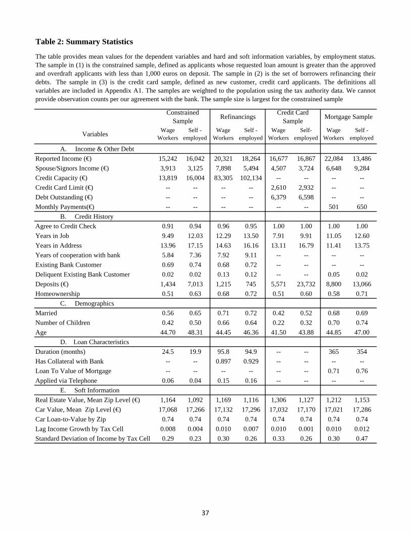
A. Income & Other Debt

Reported Income (€) 15,242 16,042 20,321 18,264 16,677 16,867 22,084 13,486

Spouse/Signors Income (€) 3,913 3,125 7,898 5,494 4,507 3,724 6,648 9,284

Credit Capacity (€) 13,819 16,004 83,305 102,134 -- -- -- --

Credit Card Limit (€) -- -- -- -- 2,610 2,932 -- --

Debt Outstanding (€) -- -- -- -- 6,379 6,598 -- --

Monthly Payments(€) -- -- -- -- -- -- 501 650

B. Credit History

Agree to Credit Check 0.91 0.94 0.96 0.95 1.00 1.00 1.00 1.00

Years in Job 9.49 12.03 12.29 13.50 7.91 9.91 11.05 12.60

Years in Address 13.96 17.15 14.63 16.16 13.11 16.79 11.41 13.75

Years of cooperation with bank 5.84 7.36 7.92 9.11 -- -- -- --

Existing Bank Customer 0.69 0.74 0.68 0.72 -- -- -- --

Deliquent Existing Bank Customer 0.02 0.02 0.13 0.12 -- -- 0.05 0.02

Deposits (€) 1,434 7,013 1,215 745 5,571 23,732 8,800 13,066

Homeownership 0.51 0.63 0.68 0.72 0.51 0.60 0.58 0.71

C. Demographics

Married 0.56 0.65 0.71 0.72 0.42 0.52 0.68 0.69

Number of Children 0.42 0.50 0.66 0.64 0.22 0.32 0.70 0.74

Age 44.70 48.31 44.45 46.36 41.50 43.88 44.85 47.00

D. Loan Characteristics

Duration (months) 24.5 19.9 95.8 94.9 -- -- 365 354

Has Collateral with Bank -- -- 0.897 0.929 -- -- -- --

Loan To Value of Mortgage -- -- -- -- -- -- 0.71 0.76

Applied via Telephone 0.06 0.04 0.15 0.16 -- -- -- --

E. Soft Information

Real Estate Value, Mean Zip Level (€) 1,164 1,092 1,169 1,116 1,306 1,127 1,212 1,153

Car Value, Mean Zip Level (€) 17,068 17,266 17,132 17,296 17,032 17,170 17,021 17,286

Car Loan-to-Value by Zip 0.74 0.74 0.74 0.74 0.74 0.74 0.74 0.74

Lag Income Growth by Tax Cell 0.008 0.004 0.010 0.007 0.010 0.001 0.010 0.012

Standard Deviation of Income by Tax Cell 0.29 0.23 0.30 0.26 0.33 0.26 0.30 0.47

Self- employed

Wage Workers

Self -employed

Table 2: Summary Statistics

VariablesWage

WorkersSelf -

employedWage

WorkersSelf -

employedWage

Workers

The table provides mean values for the dependent variables and hard and soft information variables, by employment status.The sample in (1) is the constrained sample, defined as applicants whose requested loan amount is greater than the approvedand overdraft applicants with less than 1,000 euros on deposit. The sample in (2) is the set of borrowers refinancing theirdebts. The sample in (3) is the credit card sample, defined as new customer, credit card applicants. The definitions allvariables are included in Appendix A1. The samples are weighted to the population using the tax authority data. We cannotprovide observation counts per our agreement with the bank. The sample size is largest for the constrained sample

Constrained Sample

RefinancingsCredit Card

SampleMortgage Sample

37

Table 3: True Income Estimated in Constrained Applicants Sample

Fixed Effects

Coefficien Lambda Coefficien Lambda Coefficien Lambda Coefficien LambdaReported Income*IWageWorker 0.520*** 0.505*** 0.497*** 0.483***

[0.110] [0.105] [0.107] [0.102]Reported Income*ISelf Employed*

Accounting & Financial Services 1.133*** 2.18 1.112*** 2.20 1.531*** 3.08 1.513*** 3.13[0.155] [0.153] [0.324] [0.318]

Agriculture 0.693*** 1.33 0.681*** 1.35 0.649*** 1.31 0.655*** 1.35[0.104] [0.0944] [0.192] [0.169]

Business Services 0.800*** 1.54 0.774*** 1.53 0.666*** 1.34 0.639*** 1.32[0.0815] [0.0800] [0.108] [0.105]

Construction 0.968*** 1.86 0.955*** 1.89 1.124*** 2.26 1.107*** 2.29[0.189] [0.190] [0.318] [0.316]

Doctors & Medicine 1.430** 2.75 1.412** 2.80 1.716* 3.45 1.706* 3.53[0.620] [0.615] [0.941] [0.931]

Education 1.010*** 1.94 0.999*** 1.98 1.383*** 2.78 1.371*** 2.84[0.147] [0.151] [0.346] [0.347]

Engineering & Science 1.541*** 2.96 1.524*** 3.02 2.258*** 4.54 2.223*** 4.60[0.433] [0.416] [0.658] [0.633]

Fabrication 0.869*** 1.67 0.858*** 1.70 0.896*** 1.80 0.885*** 1.83[0.120] [0.117] [0.183] [0.177]

Law 1.178*** 2.26 1.185*** 2.35 1.134*** 2.28 1.101*** 2.28[0.240] [0.240] [0.349] [0.336]

Lodging & Restaurants 0.961*** 1.85 0.973*** 1.93 1.146*** 2.30 1.134*** 2.35[0.146] [0.149] [0.327] [0.330]

Media & Art 0.962*** 1.85 0.972*** 1.93 1.075*** 2.16 1.040*** 2.15[0.127] [0.124] [0.0908] [0.0913]

Other 0.691*** 1.33 0.675*** 1.34 0.567*** 1.14 0.557*** 1.15[0.0787] [0.0784] [0.102] [0.102]

Personal Services & Pharmacy 0.803*** 1.54 0.792*** 1.57 0.757*** 1.52 0.748*** 1.55[0.0799] [0.0787] [0.103] [0.105]

Retail 0.578*** 1.11 0.574*** 1.14 0.406*** 0.82 0.409*** 0.85[0.0724] [0.0714] [0.0589] [0.0587]

Transport 0.346*** 0.67 0.340*** 0.67 0.250*** 0.50 0.252*** 0.52[0.0969] [0.0948] [0.0897] [0.0882]

The dependent variable is credit capacity defined to be total debt for individuals whose loan amount approved is lowerthan amount requested and for individuals taking out an overdraft loan without large bank checking or savings balances.Presented are the coefficients on income interacted with a wage worker dummy and income for the self-employed,specific for each occupation. Lambdas are the ratio of the coefficient on income for each of the self-employedoccupations divided by the coefficient for the wage worker. Not included in the table presentation, but included in theestimation, are all the covariates reported in column 1 of the appendix table, including borrower and loan characteristics,borrower credit history, soft information variables, year dummies, and a self-employment dummy. Model (2) includesbrach fixed effects. The occupation fixed effects models (3) include occupation fixed effects and occupation crossed withself-employment fixed effects. Model (4) includes branch fixed effects,ccupation fixed effects and occupation crossedwith self-employment fixed effects. ***, **, and * indicate significance at the 1%, 5%, and 10% levels respectively.

Dependent Variable: Credit Capacity = Outstanding Debt + Approved Loan

None BranchIndustry*Self Employment

Industry*Self Employed, Branch

(3)(2)(1) (4)

38

Table 4: True Income Estimated in Refinancings Sample

Fixed Effects

Coefficien Lambda Coefficien Lambda Coefficien Lambda Coefficien LambdaReported Income*IWageWorker 0.744*** 0.738*** 0.690*** 0.682***

[0.264] [0.210] [0.255] [0.201]Reported Income*ISelf Employed*

Accounting & Financial Services 1.379*** 1.85 1.454*** 1.97 1.329*** 1.93 1.405*** 2.06[0.326] [0.306] [0.514] [0.478]

Agriculture 0.342 -- 0.422** 0.57 0.72 -- 0.711 --[0.217] [0.214] [0.485] [0.459]

Business Services 1.425*** 1.92 1.373*** 1.86 1.319*** 1.91 1.263*** 1.85[0.284] [0.275] [0.372] [0.360]

Construction 0.618*** 0.83 0.640*** 0.87 0.555*** 0.80 0.614*** 0.90[0.130] [0.109] [0.132] [0.113]

Doctors & Medicine 1.816*** 2.44 1.936*** 2.62 1.094 -- 1.167* 1.71[0.494] [0.453] [0.674] [0.626]

Education 2.567*** 3.45 2.290*** 3.10 2.074 -- 2.388 --[0.902] [0.874] [2.439] [2.236]

Engineering & Science 1.825*** 2.45 1.866*** 2.53 2.547*** 3.69 2.569*** 3.77[0.489] [0.483] [0.777] [0.767]

Fabrication 1.948*** 2.62 1.854*** 2.51 2.188*** 3.17 2.012*** 2.95[0.239] [0.223] [0.312] [0.291]

Law 1.389*** 1.87 1.321** 1.79 1.848** 2.68 1.783* 2.61[0.487] [0.552] [0.772] [0.913]

Lodging & Restaurants 1.722*** 2.32 1.466*** 1.99 2.070*** 3.00 1.740** 2.55[0.448] [0.430] [0.801] [0.750]

Media & Art 3.539** 4.76 2.704*** 3.67 3.588** 5.20 2.611** 3.83[1.471] [0.980] [1.828] [1.285]

Other 1.012** 1.36 0.895** 1.21 0.853* 1.24 0.781* 1.15[0.408] [0.377] [0.461] [0.429]

Personal Services & Pharmacy 0.711*** 0.96 0.745*** 1.01 1.144*** 1.66 1.086*** 1.59[0.201] [0.183] [0.210] [0.195]

Retail 1.480*** 1.99 1.426*** 1.93 1.599*** 2.32 1.540*** 2.26[0.250] [0.252] [0.360] [0.372]

Transport 1.999*** 2.69 1.848*** 2.51 1.864** 2.70 1.747** 2.56[0.439] [0.445] [0.736] [0.769]

The dependent variable is credit capacity defined to be total debt for individuals whose loan amount approved is lowerthan amount requested and for individuals taking out an overdraft loan without large bank checking or savings balances.Presented are the coefficients on income interacted with a wage worker dummy and income for the self-employed,specific for each occupation. Lambdas are the ratio of the coefficient on income for each of the self-employedoccupations divided by the coefficient for the wage worker. Not included in the table presentation, but included in theestimation, are all the covariates reported in column 1 of the appendix table, including borrower and loan characteristics,borrower credit history, soft information variables, year dummies, and a self-employment dummy. Model (2) includesbrach fixed effects. The occupation fixed effects models (3) include occupation fixed effects and occupation crossed withself-employment fixed effects. Model (4) includes branch fixed effects,ccupation fixed effects and occupation crossedwith self-employment fixed effects. ***, **, and * indicate significance at the 1%, 5%, and 10% levels respectively.

None BranchIndustry*Self Employment

Industry*Self Employed, Branch

Dependent Variable: Credit Capacity = Outstanding Debt + Approved Loan(1) (2) (3) (4)

39

Table 5: True Income Estimated in Credit Card Sample

Fixed Effects

Coefficient Lambda Coefficient Lambda Coefficient Lambda Coefficient LambdaReported Income*IWageWorker 0.0381*** 0.0397*** 0.0387*** 0.0380***

[0.00674] [0.00696] [0.00687] [0.00687]Reported Income*ISelf Employed*

Accounting & Financial Services 0.0603*** 1.58 0.0591*** 1.49 0.0511*** 1.32 0.0572*** 1.50[0.0114] [0.0135] [0.0182] [0.0215]

Agriculture 0.0724*** 1.90 0.0871*** 2.19 0.130*** 3.36 0.130*** 3.42[0.0232] [0.0217] [0.0241] [0.0199]

Business Services 0.0818*** 2.15 0.0631*** 1.59 0.0855*** 2.21 0.0819*** 2.15[0.0141] [0.0133] [0.0239] [0.0221]

Construction 0.0943*** 2.48 0.0892*** 2.25 0.111*** 2.88 0.105*** 2.77[0.0133] [0.0116] [0.0179] [0.0155]

Doctors & Medicine 0.0760*** 2.00 0.0676*** 1.70 0.0709*** 1.83 0.0647*** 1.70[0.0111] [0.0105] [0.0144] [0.0131]

Education 0.149*** 3.90 0.124*** 3.12 0.192*** 4.96 0.172*** 4.51[0.0400] [0.0297] [0.0640] [0.0642]

Engineering & Science 0.0395*** 1.04 0.0385*** 0.97 0.0308** 0.79 0.0303** 0.80[0.0145] [0.0138] [0.0137] [0.0130]

Fabrication 0.0866*** 2.27 0.0875*** 2.21 0.0815*** 2.11 0.0920*** 2.42[0.0148] [0.0147] [0.0182] [0.0192]

Law 0.0906*** 2.38 0.0940*** 2.37 0.113*** 2.91 0.0955*** 2.51[0.0181] [0.0187] [0.0302] [0.0277]

Lodging & Restaurants 0.0723*** 1.90 0.0715*** 1.80 0.0876*** 2.26 0.0782*** 2.05[0.0181] [0.0171] [0.0267] [0.0250]

Media & Art 0.0695*** 1.82 0.0559*** 1.41 0.111*** 2.87 0.131*** 3.43[0.0169] [0.0177] [0.0370] [0.0341]

Other 0.0432** 1.13 0.0388** 0.98 0.0295* 0.76 0.0283* 0.74[0.0171] [0.0154] [0.0157] [0.0147]

Personal Services & Pharmacy 0.0284** 0.75 0.0250** 0.63 0.0262** 0.68 0.0240* 0.63[0.0112] [0.0118] [0.0128] [0.0143]

Retail 0.0253*** 0.66 0.0293*** 0.74 0.00972 -- 0.0179* 0.47[0.00824] [0.00835] [0.00862] [0.00989]

Transport 0.0410* 1.08 0.0393* 0.99 0.0302 -- 0.0358 --[0.0238] [0.0220] [0.0280] [0.0292]

The dependent variable is credit card limits. Presented are the coefficients on income interacted with a wage workerdummy and income for the self-employed, specific for each occupation. Lambdas are the ratio of the coefficient onincome for each of the self-employed occupations divided by the coefficient for the wage worker. Not included in thetable presentation, but included in the estimation, are all the covariates reported in column 1 of the appendix table,including borrower and loan characteristics, borrower credit history, soft information variables, year dummies, and a self-employment dummy. Model (2) includes brach fixed effects. The occupation fixed effects models (3) include occupationfixed effects and occupation crossed with self-employment fixed effects. Model (4) includes branch fixedeffects,ccupation fixed effects and occupation crossed with self-employment fixed effects. ***, **, and * indicatesignificance at the 1%, 5%, and 10% levels respectively.

None BranchIndustry*Self Employment

Industry*Self Employed, Branch

Dependent Variable: Credit Capacity = Outstanding Debt + Approved Loan(1) (2) (3) (4)

40

Table 6: True Income Estimated in Mortgage Sample

Model:

Coefficient Lambda Coefficient Lambda Coefficient LambdaReported Income*IWageWorker 0.00225*** 0.00272*** 0.00260***

[0.000359] [0.000273] [0.000274]Reported Income*ISelf Employed*

Accounting & Financial Services 0.00829*** 3.69 0.00752*** 2.76 0.00665*** 2.56[0.00159] [0.00218] [0.00218]

Agriculture 0.00428*** 1.90 -0.00662*** -2.43 -0.00592** -2.28[0.00153] [0.00246] [0.00249]

Business Services 0.00860*** 3.83 0.00558** 2.05 0.00531** 2.04[0.00274] [0.00252] [0.00252]

Construction 0.00478*** 2.13 0.00374*** 1.37 0.00360*** 1.39[0.00115] [0.00110] [0.00108]

Doctors & Medicine 0.00652*** 2.90 0.00868*** 3.19 0.00861*** 3.32[0.00147] [0.00175] [0.00173]

Education 0.00323*** 1.44 0.00277 -- 0.00267 --[0.00122] [0.00176] [0.00176]

Engineering & Science 0.00410*** 1.82 0.00443*** 1.63 0.00423*** 1.63[0.00124] [0.000921] [0.000924]

Fabrication 0.00785*** 3.49 0.00562*** 2.06 0.00544*** 2.09[0.00158] [0.000936] [0.000932]

Law 0.00381*** 1.69 0.00406** 1.49 0.00410*** 1.58[0.00119] [0.00160] [0.00158]

Lodging & Restaurants 0.00991*** 4.41 0.00282 -- 0.00235 --[0.00292] [0.00241] [0.00241]

Media & Art 0.00603 -- -0.00129 -- -0.00192 --[0.00433] [0.00540] [0.00535]

Other 0.00403*** 1.79 0.00256** 0.94 0.00231** 0.89[0.000941] [0.00101] [0.00102]

Personal Services & Pharmacy 0.00475** 2.11 0.00386** 1.42 0.00375** 1.44[0.00193] [0.00177] [0.00176]

Retail 0.00696*** 3.10 0.00347*** 1.28 0.00339*** 1.30[0.00158] [0.000906] [0.000906]

Transport 0.00464*** 2.06 0.00254 -- 0.00257 --[0.00163] [0.00216] [0.00214]

Simple OLS HeckmanHeckman, Branch Fixed

Effects

The dependent variable is is the approved monthly payment implied by the mortgage amount, duration, and interest rate.Presented are the coefficients on income interacted with a wage worker dummy and income for the self-employed, specificfor each occupation. Lambdas are the ratio of the coefficient on income for each of the self-employed occupations dividedby the coefficient for the wage worker. Not included in the table presentation, but included in the estimation, are all thecovariates reported in column 1 of the appendix table, including borrower and loan characteristics, borrower credit history,soft information variables, year dummies, and a self-employment dummy. Models (2) and (3) present the Heckman twostage results, with branch fixed effects added in model (3). ***, **, and * indicate significance at the 1%, 5%, and 10%levels respectively.

Dependent Variable: Monthly Mortgage Payments(1) (3) (4)

41

Table 7: Robustness to Wealth Entering the Adaptation Assessment at Local Branch

Lambda Low Lambda High Lambda Low Lambda High Lambda Low Lambda High

Accounting & Financial Services 3.12 3.11 1.99 2.08 1.50 1.49

Agriculture 1.31 1.36 0.68 -- 3.10 3.39

Business Services 1.35 1.36 1.77 1.86 2.10 2.15

Construction 2.31 2.33 0.93 0.89 2.64 2.76

Doctors & Medicine 3.60 3.58 1.16 1.70 1.66 1.70

Education 2.86 2.87 1.07 -- 4.37 4.48

Engineering & Science 4.66 4.65 3.91 3.80 0.75 0.79

Fabrication 1.83 1.84 2.89 2.90 2.04 2.10

Law 2.31 2.27 2.86 2.66 2.61 2.53

Lodging & Restaurants 2.36 2.35 2.63 2.55 1.95 2.07

Media & Art 2.20 2.18 4.36 4.11 3.52 3.44

Other 1.15 1.17 1.14 1.15 0.66 0.74

Personal Services & Pharmacy 1.56 1.57 1.50 1.59 0.51 0.63

Retail 0.85 0.85 2.47 2.35 0.95 --

Transport 0.51 0.52 2.38 2.47 0.93 --

Presented are the lambda ranges calculated from the estimates of columns 4 in Tables 3, 4 and 5. Specifically, for column 1, we take the estimates of column 4 from Table 3 and calculate the lambda bounds if we let the soft information of wealth affect adaptation as well as repayment adjustments made by local bank officers.

Constrained Refinancing Credit Card

(1) (2) (3)

42

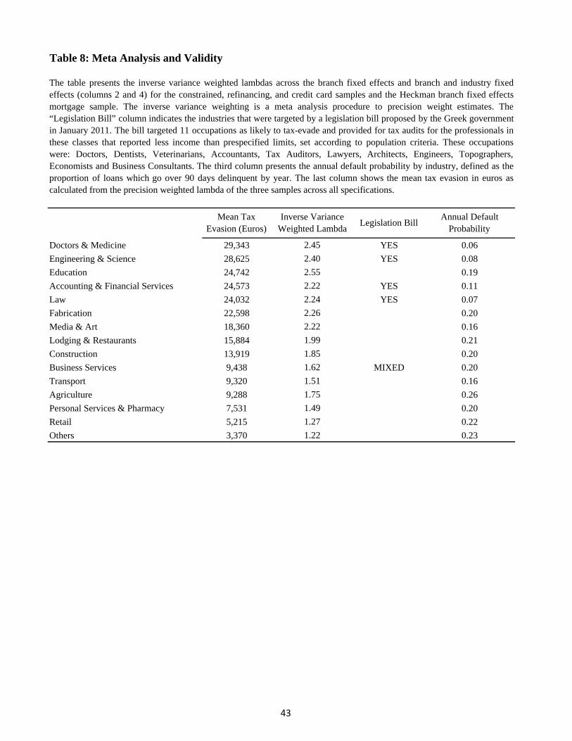
Doctors & Medicine 29,343 2.45 YES 0.06

Engineering & Science 28,625 2.40 YES 0.08

Education 24,742 2.55 0.19

Accounting & Financial Services 24,573 2.22 YES 0.11

Law 24,032 2.24 YES 0.07

Fabrication 22,598 2.26 0.20

Media & Art 18,360 2.22 0.16

Lodging & Restaurants 15,884 1.99 0.21

Construction 13,919 1.85 0.20

Business Services 9,438 1.62 MIXED 0.20

Transport 9,320 1.51 0.16

Agriculture 9,288 1.75 0.26

Personal Services & Pharmacy 7,531 1.49 0.20

Retail 5,215 1.27 0.22

Others 3,370 1.22 0.23

Table 8: Meta Analysis and Validity

The table presents the inverse variance weighted lambdas across the branch fixed effects and branch and industry fixedeffects (columns 2 and 4) for the constrained, refinancing, and credit card samples and the Heckman branch fixed effectsmortgage sample. The inverse variance weighting is a meta analysis procedure to precision weight estimates. The“Legislation Bill” column indicates the industries that were targeted by a legislation bill proposed by the Greek governmentin January 2011. The bill targeted 11 occupations as likely to tax-evade and provided for tax audits for the professionals inthese classes that reported less income than prespecified limits, set according to population criteria. These occupationswere: Doctors, Dentists, Veterinarians, Accountants, Tax Auditors, Lawyers, Architects, Engineers, Topographers,Economists and Business Consultants. The third column presents the annual default probability by industry, defined as theproportion of loans which go over 90 days delinquent by year. The last column shows the mean tax evasion in euros ascalculated from the precision weighted lambda of the three samples across all specifications.

Inverse Variance Weighted Lambda

Legislation BillAnnual Default

ProbabilityMean Tax

Evasion (Euros)

43

Table 9: Paper Trail Intensity

Tax Evasion

Lambda Scale Intensity Scale Intensity

Doctors & Medicine 29,343 2.45 0.382 M -0.412 L

Engineering & Science 28,625 2.40 0.048 M 0.555 H

Education 24,742 2.55 -0.781 L -0.474 L

Accounting & Financial Services 24,573 2.22 -0.893 L -1.105 L

Law 24,032 2.24 -1.049 L -0.169 M

Fabrication 22,598 2.26 1.382 H 0.778 H

Media & Art 18,360 2.22 -0.837 L -0.278 L

Lodging & Restaurants 15,884 1.99 0.540 H -0.263 M

Construction 13,919 1.85 0.698 H 0.340 H

Business Services 9,438 1.62 -0.948 L 0.105 M

Transport 9,320 1.51 0.081 M 0.395 H

Agriculture 9,288 1.75 0.593 H 0.684 H

Personal Services & Pharmacy 7,531 1.49 0.257 M -0.368 L

Retail 5,215 1.27 0.804 H 0.316 M

Correlation with Tax Evasion -0.248 -0.312

Correlation with Lambda -0.279 -0.303

The Table presents the results of the survey on the intensity of paper trail in various industries. Industries are sorted by theirinverse variance weighted lambdas across the four product estimations. Columns 3 and 4 report the results from Questions 1:"What percentage of expenses goes towards buying intermediate goods or services as inputs". Columns 5 and 6 report theresults from Questions 2: "How often the output is used by clients as intermediate good". Columns 3 and 5 report thedemeaned paper trail score. The higher the scale the higher the paper trail intensity. In Columns 4 and 6 we classify the papertrail scale into three levels, L-Low, M-Medium and H-High. We also present correlation of the paper trail scale with theamount of tax evasion and lambda.

Question 1: Use of Intermediate Goods as

Inputs

Question 2: Output is Intermediate Good

High Question Scale = High Paper Trail

44

Table 10: Enforcements

Panel A: Summary Statistics

MeanStandard Deviation Skewness Minimum Median Maximum Observations

Closed Cases 933.0 859.3 2.16 1 742 6,267 235Assessments 2,124,272 4,880,819 11.5 40 1,268,537 68,700,000 226Assessed/Close 3,098 20,604 14.9 12.0 1,517 311,044 226Taxfilers 23,851 18,305 1.03 676 19,083 90,532 235Percent Self Employed 0.192 0.060 3.73 0.105 0.181 0.651 235Wealth 10.68 4.64 1.08 4.50 8.94 27.48 235

The unit of observation in the table is the tax office district. Tax enforcement data are from the year 2011. Our dependent variables are the number of closes for the taxoffice for the year, the total euro value of assessments for the year, and assessments per close. Wealth is the tax authority estimate of real estate, aggregrated from zipcodes to tax district offices. It is a relative ranking and has no cardinal meaning. Percent self employed is the percent of tax filers who are either merchants or selfemployed in the tax files. Panel A presents summary statistics. Panel B presents the analyis. All estimates are OLS with all dependent and independent variables in logs,execept in the poisson specifications of columns 4-6. Wealth and %SelfEmployed are both very correlated with %SelfEmployed*Wealth (over 0.8). The VIF statistic isalways over 200. Columns 3, 6, 9, and 12 first othogonalize %SelfEmployed, Wealth, and %SelfEmployed*Wealth using the modified Gram-Schmidt procedure ofGolub and Van Loan (1996). Robust standard errors are in brackets. ***, **, and * indicate significance at the 1%, 5%, and 10% levels respectively.

45

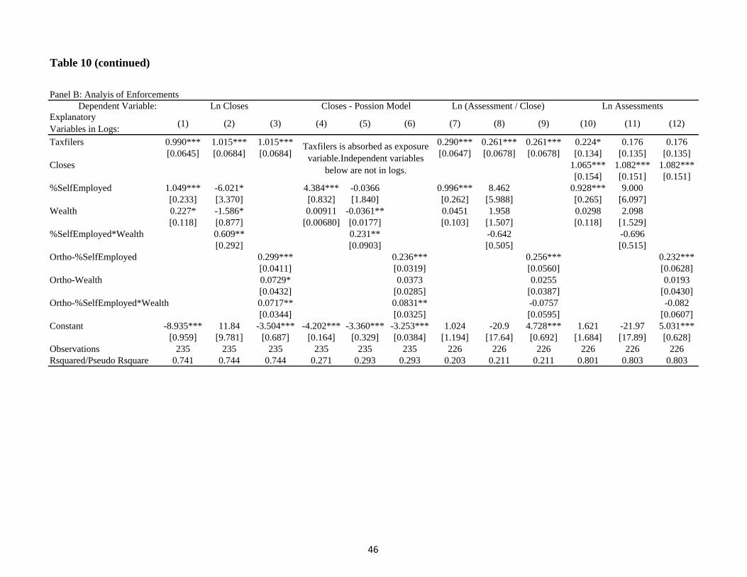
Table 10 (continued)

Panel B: Analyis of EnforcementsDependent Variable:

Explanatory Variables in Logs:

(1) (2) (3) (4) (5) (6) (7) (8) (9) (10) (11) (12)

Taxfilers 0.990*** 1.015*** 1.015*** 0.290*** 0.261*** 0.261*** 0.224* 0.176 0.176[0.0645] [0.0684] [0.0684] [0.0647] [0.0678] [0.0678] [0.134] [0.135] [0.135]

Closes 1.065*** 1.082*** 1.082***[0.154] [0.151] [0.151]

%SelfEmployed 1.049*** -6.021* 4.384*** -0.0366 0.996*** 8.462 0.928*** 9.000[0.233] [3.370] [0.832] [1.840] [0.262] [5.988] [0.265] [6.097]

Wealth 0.227* -1.586* 0.00911 -0.0361** 0.0451 1.958 0.0298 2.098[0.118] [0.877] [0.00680] [0.0177] [0.103] [1.507] [0.118] [1.529]

%SelfEmployed*Wealth 0.609** 0.231** -0.642 -0.696[0.292] [0.0903] [0.505] [0.515]

Ortho-%SelfEmployed 0.299*** 0.236*** 0.256*** 0.232***[0.0411] [0.0319] [0.0560] [0.0628]

Ortho-Wealth 0.0729* 0.0373 0.0255 0.0193[0.0432] [0.0285] [0.0387] [0.0430]

Ortho-%SelfEmployed*Wealth 0.0717** 0.0831** -0.0757 -0.082[0.0344] [0.0325] [0.0595] [0.0607]

Constant -8.935*** 11.84 -3.504*** -4.202*** -3.360*** -3.253*** 1.024 -20.9 4.728*** 1.621 -21.97 5.031***[0.959] [9.781] [0.687] [0.164] [0.329] [0.0384] [1.194] [17.64] [0.692] [1.684] [17.89] [0.628]

Observations 235 235 235 235 235 235 226 226 226 226 226 226Rsquared/Pseudo Rsquare 0.741 0.744 0.744 0.271 0.293 0.293 0.203 0.211 0.211 0.801 0.803 0.803

Ln Closes Closes - Possion Model Ln (Assessment / Close) Ln Assessments

Taxfilers is absorbed as exposure variable.Independent variables

below are not in logs.

46

Table 11: Tax Evaders and Parliamentarians Occupational Backgrounds

Tax Evasion Lambda

Parlimen-tarians Density

Cumulative Density

Represen-tatives Density

Cumulative Density

Doctors & Medicine 29,343 2.45 40 0.174 0.174 15 0.049 0.049

Engineering & Science 28,625 2.40 43 0.187 0.361 39 0.128 0.178

Education 24,742 2.55 28 0.122 0.483 28 0.092 0.270

Accounting & Financial Services 24,573 2.22 40 0.174 0.657 18 0.059 0.329

Fabrication 22,598 2.26 1 0.004 0.661 30 0.099 0.428

Media & Art 18,360 2.22 31 0.135 0.796 21 0.069 0.497

Lodging & Restaurants 15,884 1.99 3 0.013 0.809 7 0.023 0.520

Construction 13,919 1.85 2 0.009 0.817 28 0.092 0.612

Business Services 9,438 1.62 20 0.087 0.904 36 0.118 0.730

Transport 9,320 1.51 5 0.022 0.926 21 0.069 0.799Agriculture 9,288 1.75 8 0.035 0.961 18 0.059 0.859

Personal Services & Pharmacy 7,531 1.49 5 0.022 0.983 3 0.010 0.868

Retail 5,215 1.27 3 0.013 0.996 2 0.007 0.875

Other 3,370 1.22 1 0.004 1.000 38 0.125 1.000230 1.000 304 1.000

Excluded:Law 24,032 2.24 70 66Security 0 19

Distribution Tests:Pearson Chi2(12) = 117.1049 Pr = 0.000Likelihood-Ratio Chi2(12) = 137.7667 Pr = 0.000

The table reports the distribution of the occupational backgrounds of Parliament members in Greece and Canada. Industriesare sorted by their inverse variance weighted lambdas across the four product estimations. Columns 4 and 7 ("Density")present the percentage of parliament members in each occupation and columns 5 and 8 present the cumulative density. Weexclude lawyers as the natural default profession for politicians.

Greece Canada

47

48  

Appendix A1: Variable Definitions

A. Income & Other Debt   Reported Income (€) Income of the applicant as shown in the tax return form in the year of application.

Spouse Income (€) Spouse reported income based on tax return in the year of application..

Other Signors Income(€) Income of mortgage co-signors.

Credit Card Limit Approved credit card limit.

Credit Capacity (€) Total debt outstanding immediately following the loan application decision.

Debt Outstanding (€) Total debt outstanding at the time of application.

Mean Monthly Payments(€) Monthly payments of approved mortgage.

B. Credit History Agree to Credit Check The variable takes the value 1 if the applicant agrees to credit check and 0 otherwise.

Years in Job Number of years that the applicant is working under the same employer (wage workers) or is employed in the same occupation (self-employed).

Years in Address Number of years that the primary applicant resides in the same address.

Years of Cooperation with Bank

Number of years of the existing relationship of the applicant with the bank.

Existing Bank Customer The variable takes the value 1 if the applicant is an current customer of the bank and 0 otherwise.

Deliquent Existing Bank Customer

The variable takes the value 1 if the applicant is a customer of the bank but has a delayed payment in the last 6 months and 0 otherwise.

Previous Customer The variable takes the value 1 if the applicant was a customer of the bank in the past and 0 otherwise.

Previous Homeowner The variable takes the value 1 if the mortgage applicant is a homeowner and 0 otherwise.

Deposits (€) Total amount of deposits of the applicant in the bank. It includes amounts in any accounts the applicant holds with the bank (checking, savings, time-deposits, investment accounts).

Homeownership The variable takes the value 1 if the applicant is homeowner and 0 otherwise.

C. Demographics Married The variable takes the value 1 if the applicant is married and 0 otherwise.

Number of Children The number of children of the applicant at the time of the application.

Age Age of applicant at the time of the application.

D. Loan Characteristics   Duration Duration of loan (in months).

Has Collateral with Bank The applicant has posted collateral with the bank.

Loan To Value of Mortgage Ratio of the approved mortgage relative to the value of the real estate property. This variable is only available for mortgages and is calculated only for approved applications.

Applied via Telephone The applicant applied via phone call.

E. Soft Information   

Real Estate Value, Mean Zip Level (€)

The mean “presumed” real estate value of the region where the primary applicant resides (specified by zip code). “Presumed” real estate values are periodically published by tax authorities and used to determine real estate taxes. The values here come from the most recent release published in 2007.

Car Value, Mean Zip Level (€)

The mean value of automobiles by zip code, as calculated from the car loan dataset of the bank.

49  

Car Loan-to-Value by Zip Average loan-to-values of new cars by zip code

Lag Income Growth by Tax Cell

Per capital annual income growth of the prior year at the level of the zip code crossed with the four occupation-levels and the ten income decile.

Standard Deviation of Income by Tax Cell

To construct a measure of the variability of the income growth, we take into account the difference in the number of people in the zip-income decile-occupation cell. The measure is defined as the standard deviation divided by the square root of the observation count.

50  

Appendix A2: Credit History Construction

The credit history and credit performance variables were created from a set of three products: mortgages, term loans, and credit card debt. Each product included, for each customer for each month, a customer id, a record of the current month, a record of the current delay, and the amount owed on the loan. For each product a variable was generated recording how many times a customer had been late on their loan payment within the past six months, within the past 12 months, and within the past 24 months. For each span of months, we created a variable scaling the months in delay by the amount owed over the number of months in each interval. For example, this variable for the six month interval would be calculated,

six month delay amount = (six month delay* amount owed)/six

From these individual products, an average was created for the month in delay and the month in delay amount variables. The average was calculated over all the products for each customer for each month.

Besides the month in delay variables, we generated a dummy variable noting whether a customer had been delayed for a period between one and three months, for a period between three and five months, or for a period greater than six months. Additionally, a variable was created noting if a customer had ever been late on their loan, if they had ever been over a month late on their loan, or if they had every defaulted on their loan - a customer was considered to have gone into default when they were at least three months late on their loan. We then generated a second version of this variable for the entirety of a customer’s products for each month in a similar fashion to the average generated above. Finally, we created a variable noting the earliest month in which a customer was late on their loan. A second version of this variable was also generated over the entirety of each customer’s accounts for each month.

Appendix Table A1: Baseline Estimations of Credit Scoring Model without Adaptation

Sample Constrained Refinancings Credit Cards MortgagesDependent Variable Credit Capacity Credit Capacity Credit Limit Monthly Payments

Income & Other DebtReported Income 0.635*** 0.989*** 0.0433*** 0.00336***

[0.0782] [0.162] [0.00594] [0.000374]Spouse Income 0.143*** 0.503*** 0.0140***

[0.0448] [0.123] [0.00314]Other Signors Income 0.00223***

[0.000464]Debt Outstanding 0.0206***

[0.00371]Annual Payments, Balances in Bank -0.000347***

[0.000130]Annual Payments, Other Balances 0.00732***

[0.000886]Credit History

Agree to Credit Check -97.89 24,144*** -196.4 58.82[261.8] [4,272] [204.0] [47.12]

Years in Job 126.7*** 330.4* 24.60*** 1.088***[21.29] [189.5] [4.099] [0.393]

Years in Address -59.33*** -757.1*** 4.171** -0.127[12.66] [93.03] [1.885] [0.263]

Bank Relationship Years 26.29 374.4[27.81] [258.5]

Bank Score (recent variable only) 4.742[68.97]

Existing Bank Customer 1,286*** -13,554***[318.6] [4,191]

Delinquent Existing Bank Customer 4,615*** -8,812 -13.46[1,091] [5,586] [13.35]

Previous Customer 13.24[8.593]

Previous Homeowner -89.81***[7.195]

0 < Deposits < 1,000 4,601* -435.2 -153.0 -5.205[2,443] [2,587] [151.5] [12.83]

1,000 < Deposits < 2,500 15,183 17,465** 42.13 17.87[9,748] [8,397] [251.3] [22.87]

2,500 < Deposits < 8,000 11,011* 348.8 -153.6 38.33[5,916] [8,656] [263.1] [23.53]

8,000 < Deposits < 24,000 16,252* 9,113 -41.11 -16.41[9,427] [14,229] [515.6] [21.44]

24,000 < Deposits 21,537* 233.1 -97.58 104.0***[13,093] [10,449] [433.3] [22.60]

DemographicsMarried 181.1 4,096 210.7*** 22.33***

[329.7] [3,368] [59.80] [7.136]Dependents 262.3 1,525 -44.83 11.62***

[186.0] [1,437] [34.86] [3.234]35< Age < 50 911.5*** 6,212* 352.0*** -12.16

[324.1] [3,697] [43.99] [9.691]50 < Age <65 1,414*** 2,017 104.4 8.012

[446.3] [4,566] [75.42] [11.43]65 < Age <90 -298.4 11,151 -107.5 40.46

The dependant variables are credit capacity for columns 1-2, credit limits for column 3, and mortgage monthly payments for column 4.All variable definitions are given in Appendix A1. The objective of the table is to present covariate estimates, which will very closelyreflect the estimates for the main tables 3-7. Reported income in this table is not interacted with employment status. Robust standarderrors, from OLS regressions, appear in brackets. ***, **, and ** denote significance at the 1%, 5%, and 10% levels, respectively.

51

[613.1] [14,718] [170.1] [24.61]Has Collateral with Bank 8,462 17,752*** -566.0**

[6,986] [5,119] [223.8]Homeowner 1,918*** -3,638 159.1***

[235.3] [3,559] [45.53]Homeowner*Collateral 20,120* 40,907***

[11,147] [4,308]Self Employed 1,055*** 20,738*** 229.3*** 154.7***

[347.5] [2,310] [64.12] [8.616]Loan Characteristics

Applied via Telephone -2,582*** -15,298***[741.5] [3,364]

Applied via Telemarketers -2,868[2,949]

Credit Card Application -10,958***[853.5]

Overdraft Application -26,838***[2,549]

Term Loan Application 15,925**[8,124]

Term Loan Type: Balance Transfer 9,971***[878.9]

Term Loan Type: Retailer Cards 39,018***[13,891]

Line of Credit Application 15,172*[8,157]

Loan To Value of Mortgage 218.3***[10.87]

Approved Duration 435.2***[29.24]

15 Year Mortgage -126.1***[11.77]

20 Year Mortgage -143.8***[11.70]

25 Year Mortgage -122.9***[12.65]

30 Year Mortgage -123.6***[12.77]

35 Year Mortgage -103.2***[15.48]

40 Year Mortgage -96.04***[14.78]

Soft InformationCar Value by Zip -0.0539 4.875*** 0.0939*** 0.0215***

[0.121] [1.174] [0.0163] [0.00328]Car Loan-to-Value by Zip 4,035 143,370*** 384.5 48.26

[4,872] [43,518] [761.4] [147.3]Real Estate Value by Zip 1.244*** 8.934*** 0.243*** 0.0305***

[0.312] [2.590] [0.0503] [0.0101]Standard Deviation of Income by Tax Cell 3,129*** 24,410*** -27.59 40.52***

[1,002] [6,984] [93.12] [10.64]Lag Income Growth by Tax Cell 6,928 1,491 3,256*** 172.1**

[7,159] [30,980] [997.0] [87.03]

52

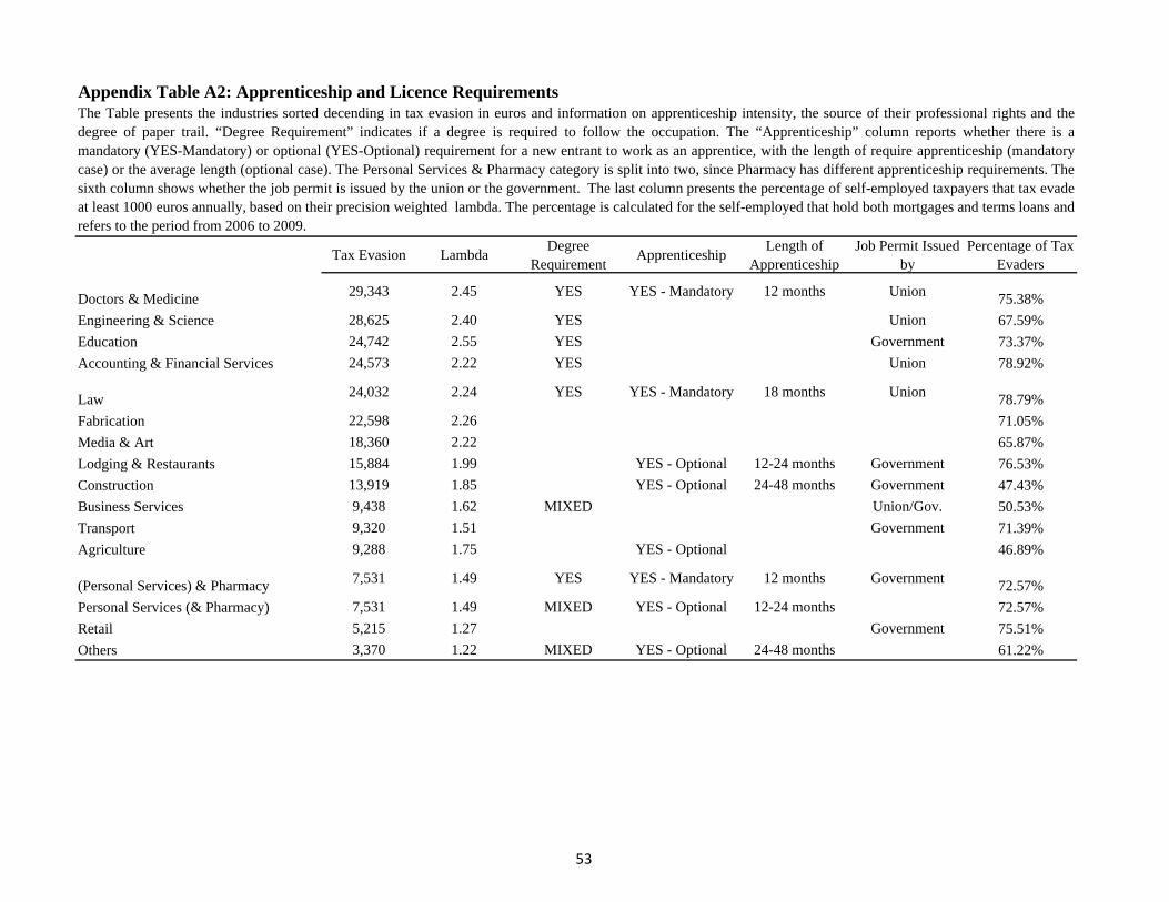
Appendix Table A2: Apprenticeship and Licence Requirements

Tax Evasion LambdaDegree

RequirementApprenticeship

Length of Apprenticeship

Job Permit Issued by

Percentage of Tax Evaders

Doctors & Medicine 29,343 2.45 YES YES - Mandatory 12 months Union 75.38%

Engineering & Science 28,625 2.40 YES Union 67.59%

Education 24,742 2.55 YES Government 73.37%

Accounting & Financial Services 24,573 2.22 YES Union 78.92%

Law 24,032 2.24 YES YES - Mandatory 18 months Union 78.79%

Fabrication 22,598 2.26 71.05%

Media & Art 18,360 2.22 65.87%

Lodging & Restaurants 15,884 1.99 YES - Optional 12-24 months Government 76.53%

Construction 13,919 1.85 YES - Optional 24-48 months Government 47.43%

Business Services 9,438 1.62 MIXED Union/Gov. 50.53%

Transport 9,320 1.51 Government 71.39%

Agriculture 9,288 1.75 YES - Optional 46.89%

(Personal Services) & Pharmacy 7,531 1.49 YES YES - Mandatory 12 months Government 72.57%

Personal Services (& Pharmacy) 7,531 1.49 MIXED YES - Optional 12-24 months 72.57%

Retail 5,215 1.27 Government 75.51%

Others 3,370 1.22 MIXED YES - Optional 24-48 months 61.22%

The Table presents the industries sorted decending in tax evasion in euros and information on apprenticeship intensity, the source of their professional rights and thedegree of paper trail. “Degree Requirement” indicates if a degree is required to follow the occupation. The “Apprenticeship” column reports whether there is amandatory (YES-Mandatory) or optional (YES-Optional) requirement for a new entrant to work as an apprentice, with the length of require apprenticeship (mandatorycase) or the average length (optional case). The Personal Services & Pharmacy category is split into two, since Pharmacy has different apprenticeship requirements. Thesixth column shows whether the job permit is issued by the union or the government. The last column presents the percentage of self-employed taxpayers that tax evadeat least 1000 euros annually, based on their precision weighted lambda. The percentage is calculated for the self-employed that hold both mortgages and terms loans andrefers to the period from 2006 to 2009.

53