Targeting Energy Efficiency in Commercial Buildings Using

Targeting Energy Efficiency in Commercial Buildings Using Advanced Billing Analysis

Kelly Kissock and Steve Mulqueen, University of Dayton

ABSTRACT

This paper describes a four-step method to analyze the utility bills and weather data from multiple buildings to target and measure the effectiveness of energy efficiency opportunities. The first step is to create a three-parameter change-point regression model of energy use versus weather for each building and type of energy. The three model parameters represent weather independent energy use, the building heating or cooling slopes and the building balance-point temperature. The second step is to drive the models with typical meteorological year (TMY2) weather data to determine Normalized Annual Consumption (NAC) for each type of energy. The third step is to create a sliding NAC with each set of 12 sequential months of utility data. The final step is to benchmark the NACs and coefficients of multiple buildings to identify average, best and worst energy performers, and how the performance of each building has changed over time. The method weather normalizes energy use, prioritizes buildings for specific energy-efficiency retrofits, and tracks weather-normalized changes in energy use. This paper describes the method, and then demonstrates the method through a case study analysis of energy use data from 14 Midwestern hospitals.

Introduction

This paper describes a four-step method to analyze the utility bills and weather data from multiple buildings to target specific energy efficiency opportunities. The method identifies buildings with the greatest energy saving opportunities from a broader group of buildings, and helps identify the best type of energy efficiency opportunity for each building. Further, it quantifies how weather-normalized energy use changes over time so that the effectiveness of energy-efficiency efforts can be measured. Thus, it is able to derive actionable information from simple utility bills.

The method of regressing utility billing data against weather data presented here builds upon the PRInceton Scorekeeping Method, PRISM [1], with a few important differences. First, the method presented here uses change-point models [2, 3] instead of the variable-base degree-day models used by PRISM. Second, this method uses TMY2 data, rather than an average of 10 years of data, as ‘typical’ weather. The interpretation of regression coefficients, also builds on early work by Goldberg and Fels [4] and by Rabl [5], Rabl et al. [6] and Reddy [7]. Principle differences between this work and the aforementioned papers are that this work seeks to use inverse modeling proactively to identify energy saving opportunities rather than retroactively to measure energy savings, and this work tracks building performance using continuous sliding analysis rather than simple pre and post-retrofit comparisons.

Overview of the Method

The first step of the method is to create statistical three-parameter models of electricity and fuel use as functions of outdoor air temperature. We call these models “energy signatures”

2-1592008 ACEEE Summer Study on Energy Efficiency in Buildings

since they summarize a building’s energy use characteristics. The three statistical-derived coefficients represent a building’s weather-independent energy use, the balance-point temperature and the overall heating or cooling coefficient.

The second step is to drive the energy signature models with typical weather data from TMY2 files [8] to determine energy use during a ‘normal’ weather year. Building energy use during a ‘normal’ weather year is called the Normalized Annual Consumption (NAC). Comparison of actual and normal annual energy consumption clearly shows when high or low energy use is caused by unusually hot or cold weather, rather than by fundamental changes in the building energy systems.

The third step is to derive an energy-signature model and NAC for each set of 12 sequential months of utility billing data. The resulting ‘sliding NACs’ show how weather-normalized energy use changes over time. Thus, NAC removes the noise associated with changing weather from the utility billing data so that the true energy using characteristics of the building can be identified. In addition, ‘sliding coefficients’ show how independent energy use, the balance temperature and the heating/cooling coefficient change over time. Using sliding analysis, building energy performance is benchmarked against previous performance to track changes in overall energy use and identify the causes of the changes.

The fourth step is to compare the NACs and coefficients of multiple buildings. In this step, building energy performance is benchmarked against other buildings. Comparison of NACs quickly identifies average, best and worst energy performers, even among buildings from different locations with different weather. Further, comparison of model coefficients indicates the root cause of the energy performance. For example, high NAC indicates high energy use, while comparative analysis of the model coefficients can indicate whether the high energy use was caused by high weather-independent energy use, indoor air temperature, a leaky building envelope or inefficient heating and air conditioning equipment.

Benchmarking NACs of multiple buildings can also target energy efficiency efforts on those buildings with the greatest energy saving potential. For example, buildings with high weather-independent electricity use are usually good targets for lighting retrofits. Buildings with unusually high or low balance temperature are usually good targets for programmable thermostats or building control systems. Buildings with high heating/cooling coefficients are good targets for envelope or high-efficiency space conditioning equipment retrofits. This information is extremely useful when conducting energy assessments, or when choosing which building to assess, since these opportunities can often be identified in advance of the site visit.

Finally, the benchmarking process quantifies the overall performance of a group of buildings, and tracks this overall performance over time. Specialized software has been developed to automate these tasks and display results graphically as well as numerically. The software significantly reduces the effort required to derive this actionable information from the utility billing data.

Description of Data and Software

The method described here uses monthly utility bills as the base energy consumption data because of their wide availability and accuracy. However, the method is easily adapted to interval or sub-metered data. In most cases, it is useful to normalize building energy use by floor area to promote accurate comparisons between buildings.

The method uses both actual and typical weather data. Actual average daily temperatures for 157 U.S. and 167 international cities from January 1, 1995 to present are available free-of-


charge over the internet from the University of Dayton Average Daily Temperature Archive [9]. The average daily temperatures posted on this site are from the National Climatic Data Center Global Summary of the Day (GSOD) dataset and are computed from 24 hourly temperature readings. The ‘typical’ weather of a given site is derived from TMY2 data files [8], which are available free-of-charge over the internet from the National Renewable Energy Laboratory. TMY2 files contain typical meteorological year data derived from the 1961-1990 National Solar Radiation Data Base. Each TMY2 files include 8,760 hourly values of solar radiation, ambient temperature, ambient humidity and wind speed that are representative of the 30 averages for the site.

The work described here used the Energy Explorer C software [10], which automates the process while providing graphical and numerical results. The software is interactive, allowing users to explore the multiple layers of information from plots of NAC distributions among multiple buildings to year-by-year views of energy-signature models using simple point-and-click features.

Step 1: Energy Signature Models

The first step is to derive statistical energy signature models of each building’s fuel and electricity use. In this analysis, the fuel and electricity use reported on the utility bills were first normalized by building floor area and by the number of days in each billing period. Thus, the base unit used throughout this paper is Btu-mo/ft2-dy for fuel and kWh-mo/ft2-dy for electricity. To derive the energy signature models, fuel use and electricity use from utility bills are entered into the program with actual average daily temperature data. Figure 1 shows seven years of monthly natural gas and electricity use data for Hospital 2.

Figure 1. Seven Years of Hospital 2 Monthly Natural Gas Use (a), and Electricity Use (b)

(a) (b)

0

30,000

60,000

90,000

120,000

Jan-95 Jan-97 Jan-99 Jan-01

NG

(the

rms/

mo)

0

400,000

800,000

1,200,000

1,600,000

1/22/95 1/22/97 1/22/99 1/22/01

Elec

(kW

h/m

o)

The program calculates the average temperature during each utility billing period. The energy use and weather data are then regressed to derive energy-signature models for each type of energy use. Figure 2 shows typical three-parameter heating (3PH) and three-parameter cooling (3PC) model for Hospital 2. In these graphs, natural gas and electricity use are plotted on the vertical axes against outdoor air temperature on the horizontal axes. The data show that fuel use is constant at high temperatures when there is minimal demand for space heating, but increases at low temperatures. Similarly, electricity use is constant at low temperatures when there is minimal demand for space cooling, but increases at high temperatures.


Figure 2. Hospital 2 Fuel Use (a) and Electricity Use (b) Plotted Against Outdoor Air Temperature with Three-Parameter Heating and Cooling Models

(a) (b)

Fi

Tcph

HS

Tcpc

Ei CS

In a 3PH model, the model coefficients are the weather-independent fuel use (Fi), the heating change-point temperature (Tcph), and the heating slope (HS). Using these coefficients, fuel use (F) can be estimated as a function of outdoor air temperature (Toa) using Equation 1. The superscript + indicates that the value of the parenthetic quantity is zero when it evaluates to a negative quantity.

F = Fi + HS (Tcph – Toa)+ (Equation 1) In a 3PC model, the model coefficients are the weather-independent electricity use (Ei),

the cooling change-point temperature (Tcpc), and the cooling slope (CS). Electricity use (E) can be estimated using Equation 2.

E = Ei + CS (Toa – Tcpc)+ (Equation 2)

Interpretation of Coefficients A primary strength of this method is that the model coefficients have physical meaning.

Thus, the coefficients can be interpreted to give insight into energy-efficiency opportunities. Fi and Ei represent weather-independent energy use. In 3PH models, Fi is frequently for

hot water or air reheat. In 3PC models, Ei is frequently for lighting, fans, electrical equipment, and cooling interior zones.

The heating/cooling slopes, HS and CS, represent a building’s overall energy response to decreasing or increasing outdoor air temperatures. The slopes incorporate external heating and cooling loads as well as the efficiencies of the heating and cooling equipment. The external heating load is dominated by the sum of conductive losses through the building envelope and the heat loss to ventilation or infiltration air. Similarly, the external cooling load is dominated by the sum of conductive heat gain through the building envelope and sensible heat gain to ventilation or infiltration air. Solar and latent cooling loads are linearly related to outdoor air temperature, and are thus accounted for in these models. Thus, the external heating and cooling coefficients, HC and CC, are:

HC = UA + V ρ cp CC = UA + V ρ cp (Equation 3)


where U is the overall building envelope conductance, A is the envelope area, V is the ventilation or infiltration flow rate, ρ is the density of air and cp is the specific heat of air.

The heating/cooling slopes, HS and CS, are the quotients of the external heating and cooling coefficients and the efficiency of the space heating/cooling equipment efficiency, ήh or ήc (Equation 4).

HS = HC / ήh CS = CC / ήc (Equation 4) The balance-point temperature, Tb, represents the outdoor air temperature below or

above which space conditioning begins. Tb is a function of the thermostat set-point temperature, Tsp, the internal loads from electricity use, solar gain and people, Qi, and the external heating or cooling coefficients (Equation 5).

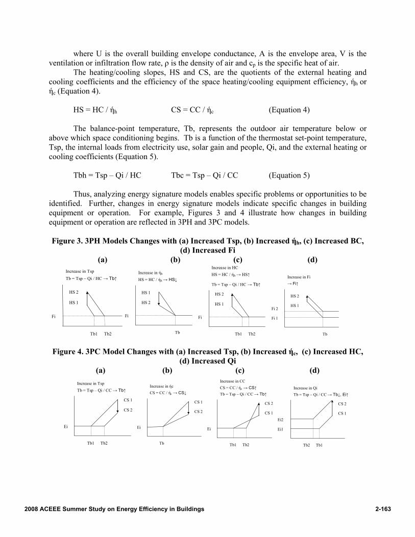
Tbh = Tsp – Qi / HC Tbc = Tsp – Qi / CC (Equation 5) Thus, analyzing energy signature models enables specific problems or opportunities to be

identified. Further, changes in energy signature models indicate specific changes in building equipment or operation. For example, Figures 3 and 4 illustrate how changes in building equipment or operation are reflected in 3PH and 3PC models.

Figure 3. 3PH Models Changes with (a) Increased Tsp, (b) Increased ήh, (c) Increased BC,

(d) Increased Fi (a) (b) (c) (d)

Tb1 Tb2

Fi

Increase in Tsp Tb = Tsp – Qi / HC → Tb↑

HS 2

HS 1

Tb

Fi

Increase in ήh HS = HC / ήh → HS↓

HS 1

HS 2

Tb2

Fi

Increase in HC

Tb = Tsp – Qi / HC → Tb↑

HS 2

HS 1

HS = HC / ήh → HS↑

Tb1 Tb

Fi 1

Increase in Fi → Fi↑

HS 2

HS 1 Fi 2

Figure 4. 3PC Model Changes with (a) Increased Tsp, (b) Increased ήc, (c) Increased HC, (d) Increased Qi

(a) (b) (c) (d)

Tb1 Tb2

Ei

Increase in Tsp Tb = Tsp – Qi / CC → Tb↑

CS 1

CS 2

Tb

Ei

Increase in ήcCS = CC / ήc → CS↓

CS 1

CS 2

Tb1 Tb2

Ei

Increase in CCCS = CC / ήc → CS↑

CS 2

CS 1

Tb = Tsp – Qi / CC → Tb↑

Tb2 Tb1

Ei1

Increase in Qi

CS 2

CS 1

Tb = Tsp – Qi / CC → Tb↓, Ei↑

Ei2


Step 2: Normalize Annual Energy Consumption

Utility bills indicate the actual energy consumption during a billing period, which, in most cases, is influenced by the weather. Therefore, assessing a building’s energy performance by simply examining utility billing data is difficult because billing energy consumption is affected by weather. Similarly, it is difficult to compare the energy performance of buildings located in different climates by comparing utility billing data. Both of these problems can be eliminated by driving energy signature models with “typical” weather from a single location. The resulting annual energy use is called the Normalized Annual Consumption, (NAC). To calculate the NAC, the energy signature models developed in Step 1 are driven with typical weather data from TMY2 files.

Figure 5 shows monthly actual and weather-normalized natural gas use over seven years for Hospital 2. The actual consumption is represented by the continuous line and the normalized consumption is characterized by the dashed line. The differences between actual and normalized consumption are caused by abnormally warm or cold weather. Thus, NAC represents a noise-free signal of building energy performance by removing the effect of abnormal weather. As such, NAC reveals the true energy characteristics of buildings, and allows comparison of building energy use between buildings in different climates and over time.

Figure 5. Time Trends of Hospital 2 Monthly Fuel Use and Weather-Normalized Fuel Use

Step 3: Sliding NAC Analysis

Changes in a building’s energy characteristics can be compared by calculating the buildings’ NAC during sequential 12-month periods. This is called a ‘sliding’ NAC analysis. To do so, an energy-signature model is created for each set of 12 sequential months, and then driven with typical weather from a TMY2 file to create a sequence of NACs. Figure 6 shows how the building’s energy signature model and NAC are computed for sequential 12-month data periods over two years. The sliding NAC analysis illustrates how the building’s fundamental energy use characteristics change over time. When these changes are caused by energy conservation retrofits, this sliding analysis provides an accurate measurement of the energy savings.


Figure 6. Graphical Representation of Sliding NAC

To illustrate the power of the sliding NAC analysis, consider Figure 7 which shows results from a sliding analysis of Hospital 2 fuel use. In Figure 7a, the dashed line is the actual annual consumption (AC) and the solid line is the NAC of natural gas over seven years. At first, both AC and NAC decrease substantially indicating a successful energy efficiency measure. However, during subsequent years the AC remains constant while the NAC slowly increases. Thus, analysis of AC alone would miss this “take back affect” in which the effectiveness of the initial energy efficiency measure was diminished.

Figure 7. Time Trends of Fuel a) NAC and AC, b) NAC and HS, c) NAC and Tbh, and d)

NAC and Fi for Hospital 2 a)

4,000

4,500

5,000

5,500

6,000

6,500

1/1/1995 12/31/1996 12/31/1998

NA

C (u

nits

/yr)

4,000

4,500

5,000

5,500

6,000

6,500

AC

(uits

/yr)

NAC AC

b)

4,0004,500

5,000

5,5006,000

6,500

1/1/1995 12/31/1996 12/31/1998

NA

C (u

nits

/yr)

0

5

10

15

20

HS

(uni

ts/y

r-F)

NAC HS

c)

4,000

4,500

5,000

5,500

6,000

6,500

1/1/1995 12/31/1996 12/31/1998

NA

C (u

nits

/yr)

35

45

55

65

75

85

Tb (F

)

NAC Tb

d)

4,000

4,500

5,000

5,500

6,000

6,500

1/1/1995 12/31/1996 12/31/1998

NA

C (u

nits

/yr)

100

150

200

250

300

Fi (u

nits

/yr)

NAC Fi

More information can be obtained by analyzing the values of the model coefficients over

time. For example, the initial decrease in natural gas NAC for this building may have been caused by a reduction in the external heating coefficient caused by increased space heating equipment efficiency or decreased ventilation air. However, Figure 7b shows that heating slope (HS) was about the same before and after the large decrease in NAC. (The short term increase and decrease in balance temperature over this time interval was caused by time lag effects during changing NAC, and do not represent actual changes.) This indicates that the decrease was not caused by increased space heating equipment efficiency or decreased ventilation air. Figure 7c shows a slight decline in balance temperature and Figure 7d shows a decrease in weather


independent fuel use. Thus, the natural gas savings were caused by a reduction in balance temperature and a reduction in weather-independent fuel use. Disaggregation of the savings shows that about 1/3 of the savings were from the decrease in weather-independent fuel use and 2/3 of the savings were from the lower balance temperature [11]. These changes could have resulted from reduced set-point temperatures, decreased hot water energy use or decreased air reheat. This example demonstrates how sliding NAC and coefficient analysis can provide a lens through which a building’s fundamental energy performance can be understood.

Step 4: Benchmarking NAC and Coefficients

In the fourth step of this method, the NAC and the model coefficients are benchmarked against other buildings to identify best and worst energy performers. One way to convey this information is to plot NAC versus increase in NAC for multiple buildings. In this paper, change in NAC, or any other statistic, is always defined to be the increase, as shown in Equation 6.

ΔNAC = (NAC_n – NAC_1) / NAC_1 (Equation 6) For example, Figure 8a shows NAC on the horizontal axis and change in NAC on the

vertical axis for 14 Midwestern hospitals. Buildings on the right side of the chart are the biggest fuel users and buildings on the left are the lowest. Buildings near the top of the chart have experienced the greatest increase in NAC, while the NACs of buildings near the bottom have decreased. The mean NAC and change in NAC are shown as lines through the center of each distribution.

This graph conveys a wealth of actionable information for energy managers or analysts. For example, on the horizontal axis, high energy buildings are targets for energy efficiency retrofits, while the low energy buildings to the left can serve as examples of what can be achieved. Similarly, buildings with large energy increases near the top of the graph may be experiencing equipment malfunctions or inadvertent changes in operations, while buildings with declining energy use near the bottom of the graph are examples of improving energy efficiency. Mean NAC, drawn as a vertical line, defines the center of the distribution and provides a metric for defining “typical” performance. Mean change in NAC, drawn as a horizontal line, indicates the magnitude of change in the energy performance of the entire group of buildings, and measures the success of energy-efficiency efforts across all buildings.

Figure 8. a) Fuel NAC versus ΔNAC, and b) HS versus ΔHS for 14 Hospitals

a)

Smallest Energy Users

Biggest Energy Increase

Biggest Energy Decrease

Biggest Energy Users

b)

Biggest Slope Decrease

Smallest Slope Biggest Slope

Biggest Slop Increase


Similar plots can be constructed for the model coefficients. As in the case of a single building, analysis of the model coefficients shows why and how NAC has changed. For example, Figure 8b shows HS on the horizontal axis and change in HS on the vertical axis for 14 Midwestern hospitals. Buildings on the right have the largest heating slopes and are targets for building envelope and space conditioning equipment retrofits, while buildings on the left demonstrate best practices. Similarly, buildings near the top have experienced significant deterioration in the building envelope or space conditioning equipment. Case Study of Midwestern Hospitals

The method is demonstrated in the following case study of 14 hospitals located in Chicago, IL and Milwaukee, WI. Building floor areas range from 202,428 ft² to 1,426,297 ft². The primary heating source for these buildings are natural gas fired boilers. The primary cooling sources for these buildings are electric centrifugal chillers. In addition to electric chillers, three buildings also have absorption chillers. This data set provides a good test for targeting energy efficiency and determining energy efficient changes.

The base data were derived from monthly billing information from 1995 to 2008; however, the number of bills available varied from a minimum of 2 years to a maximum of 8 years. Actual weather data were obtained from the Average Daily Temperature Archive [9]. All energy use data were area normalized using the respective building’s area. To determine NAC all energy signature models were driven with TMY2 data for Chicago, IL. This process enables the energy performance of buildings in different locations and with billing data from different time periods to be accurately compared.

R² values for 3PH energy signature models ranged from about 0.80 to 1.0 with a mean value of about 0.90. R² values for 3PC energy signature models ranged from about 0.60 to 1.0 with a mean value of about 0.90. The relatively high R2 values show that the models explain most of the variation in energy use. Heating R² values are typically higher than cooling R² values because space heating represents a higher fraction of total natural gas use than space cooling represents of total electricity use.

Multi-Site Electricity Use Comparisons

Figure 9 shows multi-site comparisons of electricity NAC and 3PC model coefficients. In each case, the value of the NAC or coefficient is shown on the horizontal axis and the increase is on the vertical axis. Inspection of the multisite NAC graphs quickly identifies best and worse overall energy performance across the sample. Similarly, inspection of the coefficient charts lends additional insight into best and worst independent and weather dependent building characteristics. This information allows managers or analysts to target energy efficiency efforts on the most promising buildings, and on the most promising specific areas (independent, envelope-HVAC efficiency, or building temperature control) for each building. The mean of the NAC or coefficients, and mean of the increase of coefficients are shown as dark lines. This allows managers or analysts to quantify the overall progress of energy efficiency initiatives.


Figure 9. Electricity (a) NAC versus ∆NAC, (b) Ei versus ∆Ei, (c) CS versus ∆CS, and (d) Tbc versus ∆Tbc for 14 Hospitals

(a) (b)

Smallest Energy Users

Biggest Energy Decrease

Biggest Energy Increase

Biggest Energy Users

Smallest Eind Users

Biggest Eind

Biggest Eind Decrease

Biggest Eind Increase

(c) (d)

Biggest Slop Increase

Biggest Slope

Biggest Slope Decrease

Smallest Slope

Biggest Tb Increase

Biggest Tb

Biggest Tb Decrease

Smallest Tb

Single-Site Electricity Use In Figure 9c, the hospital with the largest decrease in cooling slope is Hospital 6. Figure

10 shows time trends of NAC and cooling slope. The correlation between cooling slope and NAC is clear; both reductions in NAC resulted from reductions in the cooling slope. Independent electricity use and balance temperature remain approximately constant. The temporary instability in the slope coefficient is caused by a time delay in which the coefficient becomes unstable until a full year of energy use data with the retrofit is modeled. Decreasing cooling slope indicates an improvement in the building envelope or the energy efficiency of the cooling system. In this case, both reduction in NAC were caused by chiller retrofits in which old chillers were replaced by high-efficiency chillers. Figure 11 shows 3PC models from before and after the second chiller retrofit, and clearly indicates the decrease in cooling slope.


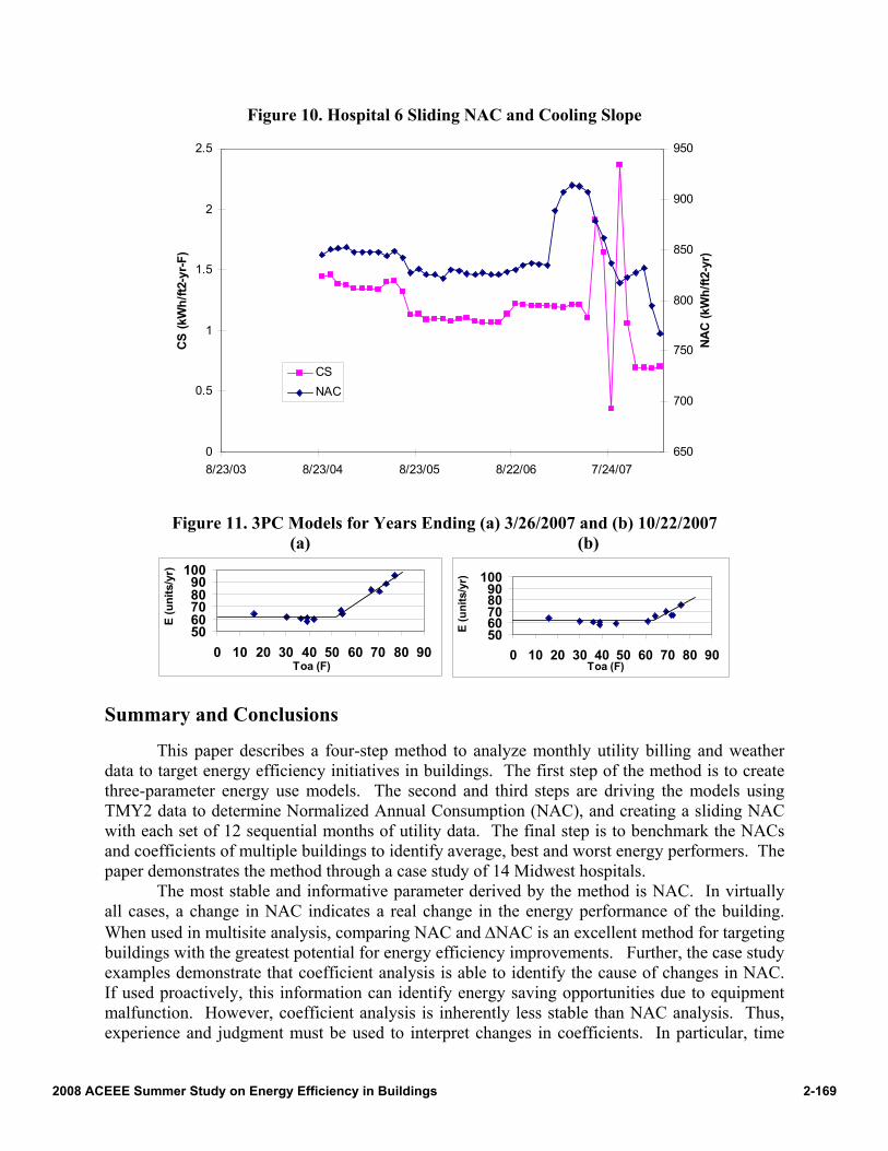
Figure 10. Hospital 6 Sliding NAC and Cooling Slope

0

0.5

1

1.5

2

2.5

8/23/03 8/23/04 8/23/05 8/22/06 7/24/07

CS

(kW

h/ft2

-yr-F

)

650

700

750

800

850

900

950

NA

C (k

Wh/

ft2-y

r)

CSNAC

Figure 11. 3PC Models for Years Ending (a) 3/26/2007 and (b) 10/22/2007 (a) (b)

5060708090

100

0 10 20 30 40 50 60 70 80 90Toa (F)

E (u

nits

/yr)

5060708090

100

0 10 20 30 40 50 60 70 80 90Toa (F)

E (u

nits

/yr)

Summary and Conclusions

This paper describes a four-step method to analyze monthly utility billing and weather data to target energy efficiency initiatives in buildings. The first step of the method is to create three-parameter energy use models. The second and third steps are driving the models using TMY2 data to determine Normalized Annual Consumption (NAC), and creating a sliding NAC with each set of 12 sequential months of utility data. The final step is to benchmark the NACs and coefficients of multiple buildings to identify average, best and worst energy performers. The paper demonstrates the method through a case study of 14 Midwest hospitals.

The most stable and informative parameter derived by the method is NAC. In virtually all cases, a change in NAC indicates a real change in the energy performance of the building. When used in multisite analysis, comparing NAC and ΔNAC is an excellent method for targeting buildings with the greatest potential for energy efficiency improvements. Further, the case study examples demonstrate that coefficient analysis is able to identify the cause of changes in NAC. If used proactively, this information can identify energy saving opportunities due to equipment malfunction. However, coefficient analysis is inherently less stable than NAC analysis. Thus, experience and judgment must be used to interpret changes in coefficients. In particular, time


lag effects can cause instability in the coefficients which do not reflect actual changes in building energy performance. Moreover, our preliminary experience suggests that in commercial buildings, slope and independent energy use are better indicators of real changes in buildings than balance-point temperature. Future work seeks to improve our abilities to correctly interpret model coefficients and to further identify both the strengths and limitations of the method.

References

[1] Fels, M., 1986, Energy and Buildings: Special Issue Devoted to Measuring Energy Savings: The Scorekeeping Approach, Vol. 9, Nums 1 & 2, February.

[2] Kissock, K., Reddy, A. and Claridge, D., 1998. "Ambient-Temperature Regression Analysis for Estimating Retrofit Savings in Commercial Buildings", ASME Journal of Solar Energy Engineering, Vol. 120, No. 3, pp. 168-176.

[3] Kissock, J.K., Haberl J. and Claridge, D.E., 2003. “Inverse Modeling Toolkit (1050RP): Numerical Algorithms”, ASHRAE Transactions, Vol. 109, Part 2.

[4] Goldberg, M. and Fels, M., 1986, “Refraction of PRISM Results in Components of Saved Energy”, Energy and Buildings, Vol. 9, Nums 1 & 2, February.

[5] Rabl, A., 1988, "Parameter Estimation in Buildings: Methods for Dynamic Analysis of Measured Energy Use", ASME Journal of Solar Energy Engineering, Vol. 110, pp. 52 - 62.

[6] Rabl, A., Norford, L. and Spadaro, J., 1986?, "Steady State Models for Analysis of Commercial Building Energy Data", Proceedings of the ACEEE Summer Study on Energy Efficiency in Buildings, Pacific Grove, CA, August, pp. 9.239-9.261.

[7] Reddy, A., 1989, "Identification of Building Parameters Using Dynamic Inverse Models: Analysis of Three Occupied Residences Monitored Non-Intrusively", Princeton University, Center for Energy and Environmental Studies Report No. 236, Princeton, NJ.

[8] National Renewable Energy Laboratory, 1995, “User’s Manual for TMY2s”, http://rredc.nrel.gov/solar/old_data/nsrdb/tmy2/.

[9] Kissock, J.K., 1999. “UD EPA Average Daily Temperature Archive”, (http://www.engr.udayton.edu.weather).

[10] Kissock, J. K, Energy Explorer C, copyright 2006 Kelly Kissock.

[11] Kissock, J.K. and Eger, C., 2008, “Measuring Industrial Energy Savings”, Journal of Applied Energy, Vol. 85, Issue 5, pp. 347-361, May.


Documents

Targeting Energy Efficiency in Commercial Buildings Using