Embed Size (px)
Citation preview
Tangible ways towards climate protection in the European Union
(EU Long-term scenarios 2050)
Benjamin Pfluger, Frank Sensfuß, Gerda Schubert, Johannes Leisentritt
Financed by the Federal Ministry for the Environment, Nature Conservation and Nuclear
Safety
Karlsruhe, 19 September 2011

Institute
Fraunhofer Institute for Systems and Innovation Research ISI
Breslauer Str. 48, 76139 Karlsruhe, Germany
www.isi.fraunhofer.de
Contacts
Dr. rer. pol. Frank Sensfuß
Telephone: 49 (0)721 6809 133, Fax 0721/809-272
e-mail: [email protected]
Dipl.-Wirt.-Ing. Benjamin Pfluger
Telephone: +49 (0)721 6809 163, Fax 0721/809-272
e-mail: [email protected]
Fraunhofer ISI: EU Long-term scenarios 2050 iii
Executive Summary
Scope of the study: This study investigates concrete and realizable ways towards a Euro-
pean electricity sector in line with the goal of keeping global warming below 2°C. It ana-
lyzes the development of the electricity sector in the EU 27, Norway and Switzerland up to
the year 2050. The study is carried out by the Fraunhofer Institute for Systems and Innova-
tion Research ISI for the German Federal Ministry for the Environment, Nature Conserva-
tion and Nuclear Safety.
Focus: The study focuses on two major aspects. First of all, it provides a detailed picture of
possible developments in the electricity sector with low carbon emissions and high diffu-
sion of renewable electricity generation. The analysis is carried out on an hourly basis for
three year-round meteorological datasets in order to ensure the reliability of the system.
Secondly, the study analyzes the impacts of increased efficiency in electricity consumption
on the required infrastructure, the structure of the electricity supply and the cost of the
system. Therefore, two scenarios are developed. Scenario A “High efficiency” presumes a
very ambitious reduction of electricity demand, based on the ADAM study (Jochem &
Schade 2009). The second Scenario B “Moderate efficiency” is based on the electricity
demand of the TRANS-CSP study (DLR 2006), projecting higher electricity consumption
than in Scenario A. In both scenarios, a cap of 75 Mt is applied to the average annual CO2
emissions in 2050, relating to a 95% reduction compared to 1990 levels. Both scenarios
do not rely on additional nuclear capacity and CCS in the electricity sector, since both op-
tions are connected with substantial political, economic and technical uncertainties. In
both scenarios the given CO2 target is achieved without relying on these technologies.
Main findings: The study shows in detail that an ambitious greenhouse gas reduction
can be achieved solely by high diffusion levels of renewable electricity generation of more
than 90%.
A cost-efficient solution for the given task requires considerable increases in the transmis-
sion capacity of the electricity grid.
The demand for additional storage capacity is limited if the electricity grid is strong
enough and renewable electricity generation is adequate for the given emission cap.
A balanced regional distribution of renewable generation leads to lower total system costs
than a distribution which is based on minimization of RES-E generation costs.
Increased efforts to reach a high efficiency in electricity demand can be valuable, since
lower demand reduces the cost of electricity supply considerably. This also includes less
need for sometimes contested infrastructures such as power lines and electricity storage
facilities.
iv Fraunhofer ISI: EU Long-term scenarios 2050
Table of content
1 Introduction .......................................................................................................... 12
1.1 Approach ...................................................................................................... 12
2 Definition of exogenous input parameters ........................................................ 14
2.1 Electricity demand ........................................................................................ 14
2.2 Fuel prices and CO2 prices ........................................................................... 16
2.3 CO2 cap ........................................................................................................ 17
3 Development of renewable electricity generation ............................................ 18
3.1 Calibration and iteration procedure .............................................................. 19
3.2 Development of specific investment costs .................................................... 22
3.3 Development of utilized renewable generation potential .............................. 23
3.4 Regional distribution of renewable electricity generation ............................. 26
4 Feed-in profiles for photovoltaic and wind power ............................................ 29
4.1 Profiles for photovoltaic ................................................................................ 30
4.1.1 Approach of the model ISI-PV-Europe ................................................ 32
4.1.2 Model evaluation ................................................................................. 36
4.2 Profiles for wind power ................................................................................. 40
4.2.1 Approach of the model ISI-Wind-Europe ............................................ 41
4.2.2 Model evaluation and calibration ......................................................... 45
5 Optimization of the power sector ....................................................................... 48
5.1 Optimization problem .................................................................................... 48
5.2 Technological assumptions .......................................................................... 50
5.2.1 Conventional power plants .................................................................. 50
5.2.2 Grid expansions .................................................................................. 52
5.2.3 Storage facilities .................................................................................. 52
6 Results .................................................................................................................. 55
6.1 Renewable electricity utilization .................................................................... 55
6.2 Conventional power plants ........................................................................... 57
6.3 CO2 emissions .............................................................................................. 61
6.4 Interconnector capacity ................................................................................ 63
6.4.1 Implications for national transport grids and electricity distribution grids .................................................................................................... 67
6.5 Storage capacity ........................................................................................... 68
6.6 Costs 70
Fraunhofer ISI: EU Long-term scenarios 2050 5
7 Matching supply and demand in every hour ..................................................... 75
8 Sensitivity analysis .............................................................................................. 81
8.1 Meteorological dataset ................................................................................. 81
8.1.1 Renewable electricity generation ........................................................ 81
8.1.2 CO2 Emissions .................................................................................... 83
8.1.3 Infrastructure ....................................................................................... 84
8.2 Renewable energy technology parameters .................................................. 85
8.3 Renewable energy imports (e.g. Desertec) .................................................. 85
8.4 Availability of CCS and nuclear power ......................................................... 86
8.5 Fuel prices .................................................................................................... 86
8.6 CO2 prices .................................................................................................... 86
8.7 CO2 cap ........................................................................................................ 87
8.8 Volume of RES-E generation ....................................................................... 87
8.9 Demand-side management .......................................................................... 88
9 Conclusions and outlook .................................................................................... 88
10 Appendix .............................................................................................................. 90
11 Literature ............................................................................................................ 107
vi Fraunhofer ISI: EU Long-term scenarios 2050
Figures
Figure 1: Step-wise approach of the scenario modelling in this study ......................... 14
Figure 2: Development of net electricity demand in the scenarios .............................. 15
Figure 3: Development of fuel prices and CO2 prices in both scenarios ..................... 17
Figure 4: Impact of RES-E volume on total system cost (Scenario A) ........................ 21
Figure 5: Impact of RES-E volume on total system cost (Scenario B) ........................ 21
Figure 6: Development of specific investments for important RES-E Technologies ................................................................................................ 23
Figure 7: Generation potential of renewables in Scenario A ....................................... 24
Figure 8: Generation potential of renewables in Scenario B ....................................... 25
Figure 9: Regional distribution of wind onshore capacity installed in 2050 in Scenario A (in GW) ....................................................................................... 27
Figure 10: Regional distribution of wind offshore capacity installed in 2050 in Scenario A (in GW) ....................................................................................... 28
Figure 11: Regional distribution of PV capacity installed in 2050 in Scenario A (in GW) ......................................................................................................... 28
Figure 12: Spectral distribution depending on the position of the sun on a clear day ................................................................................................................ 31
Figure 13: Relative conversion efficiency of modules at 50°C compared to the same modules at standard testing conditions (25°C) ................................... 32
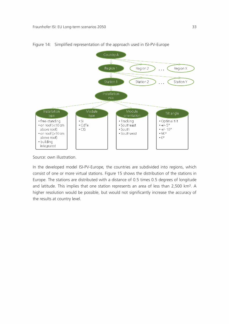
Figure 14: Simplified representation of the approach used in ISI-PV-Europe ............... 33
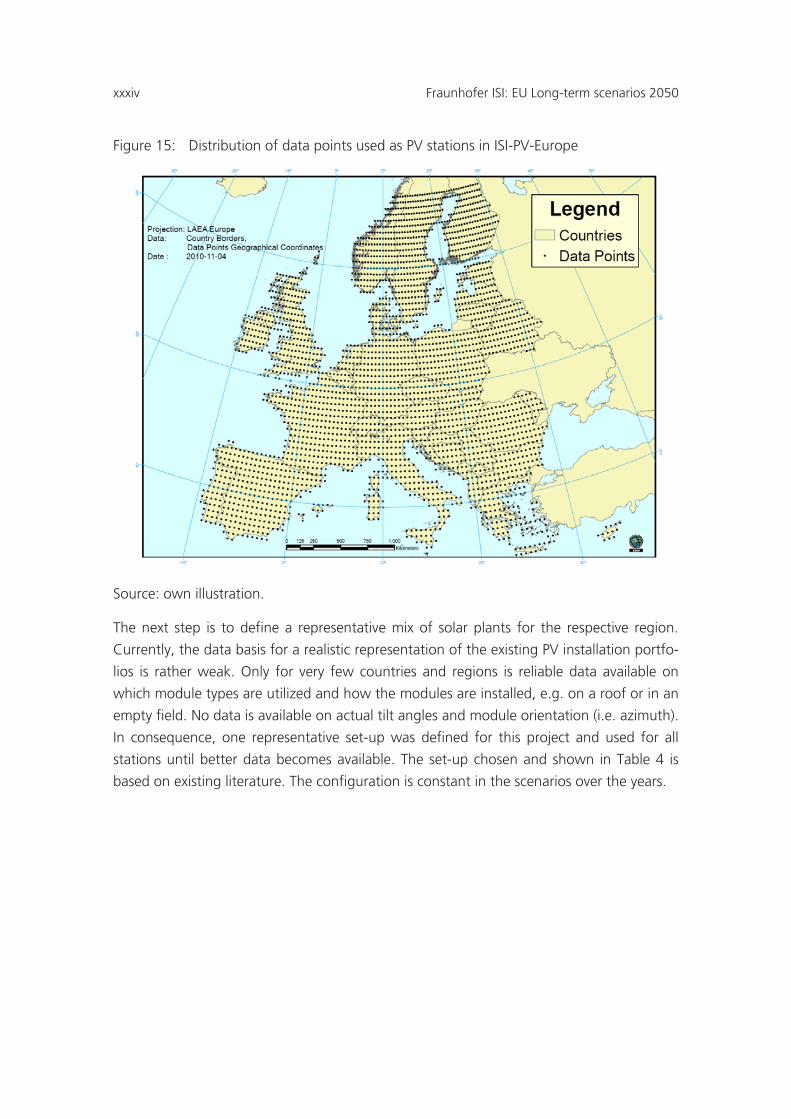
Figure 15: Distribution of data points used as PV stations in ISI-PV-Europe ................ 34
Figure 16: Measured and calculated generation for a 1.32 MWp plant in Dresden in September 2008 ......................................................................... 37
Figure 17: Comparison of the yearly sums of global irradiation: In the background the average of the years 1981-1990, the dots show the values of 2008 provided by SoDa ................................................................. 40
Figure 18: Positions of the weather stations that provided input data for ISI-Wind-Europe ................................................................................................. 41
Figure 19: Average development of the wind speed at different heights at a measuring station in Cabouw, the Netherlands. The y-axis shows the wind speed, the x-axis the hour of the day ............................................. 42
Figure 20: Allocation of the installed capacity to the measurement stations ................. 45
Fraunhofer ISI: EU Long-term scenarios 2050 7
Figure 21: Comparison of published and modelled generation profile for Germany, September 2008 .......................................................................... 46
Figure 22: Possible specific investment ranges for 8 hours of storage for pumped hydro electric storage (PHES), (advanced adiabatic compressed air energy storage [(AA-)CAES] and hydrogen storages (H2) ............................................................................................................... 54
Figure 23: Development of utilized RES-E generation .................................................. 56
Figure 24: Development of RES-E curtailment .............................................................. 57
Figure 25: Development of installed conventional capacity in Scenario A .................... 58
Figure 26: Development of installed conventional capacity in Scenario B .................... 59
Figure 27: Development of conventional generation in Scenario A ............................... 60
Figure 28: Development of conventional generation in Scenario B ............................... 61
Figure 29: Average utilization of power plants in Scenario A and B .............................. 61
Figure 30: Average annual CO2 emissions .................................................................... 62
Figure 31: Development of cumulated CO2 emissions .................................................. 63
Figure 32: Development of interconnector capacity in both scenarios .......................... 64
Figure 33: Additional interconnector capacities installed in 2050 in Scenario A expressed in MW (rounded to hundreds) ..................................................... 66
Figure 34: Additional interconnector capacities installed in 2050 in Scenario B expressed in MW (rounded to hundreds) ..................................................... 67
Figure 35: Development of storage capacity ................................................................. 69
Figure 36: Development of total costs per year ............................................................. 71
Figure 37: Development of cumulated costs ................................................................. 72
Figure 38: Development of specific cost ........................................................................ 73
Figure 39: Development of costs in Scenario A ............................................................. 74
Figure 40: Development of cost in Scenario B .............................................................. 75
Figure 41: Example of the hourly matching between supply and demand for Germany calendar week 42 in 2050, with weather settings of 2008 ............ 76
Figure 42: Example of the hourly matching between supply and demand for Spain in calendar week 27 in 2050, with weather settings of 2008 .............. 77
Figure 43: Example of the hourly matching between supply and demand for Norway in calendar week 29 in 2050, with weather settings of 2008 ........... 78
viii Fraunhofer ISI: EU Long-term scenarios 2050
Figure 44: Example of the hourly matching between supply and demand for the United Kingdom in calendar week 29 in 2050, with weather settings of 2008 ......................................................................................................... 79
Figure 45: Example of the hourly matching between supply and demand for Romania in calendar week 29 in 2050, with weather settings of 2008 ......... 80
Figure 46: Impact of meteorological dataset on RES-E generation potential in 2050 ............................................................................................................. 82
Figure 47: Impact of meteorological dataset on RES-E curtailment in Scenario B ................................................................................................................... 83
Figure 48: Impact of meteorological dataset on CO2 emissions in 2050 ....................... 84
Figure 49: Installed wind onshore capacity in 2050 (Scenario A) .................................. 95
Figure 50: Installed wind offshore capacity in 2050 (Scenario A) .................................. 95
Figure 51: Installed biommass and biogas capacity in 2050 (Scenario A) .................... 96
Figure 52: Installed hydropower capacity in 2050 (Scenario A) .................................... 96
Figure 53: Installed photovolatics capacity in 2050 (Scenario A) .................................. 97
Figure 54: Installed capacity of other technologies (biowaste, sewage and landfill gas, wave, tidal, geothermal and solar thermal) in 2050 (Scenario A) .................................................................................................. 97
Figure 55: Installed wind onshore capacity in 2050 (Scenario B) .................................. 98
Figure 56: Installed wind offshore capacity in 2050 (Scenario B) .................................. 98
Figure 57: Installed biommass and biogas capacity in 2050 (Scenario B) .................... 99
Figure 58: Installed hydropower capacity in 2050 (Scenario B) .................................... 99
Figure 59: Installed photovolatics capacity in 2050 (Scenario B) ................................ 100
Figure 60: Installed capacity of other technologies (biowaste, sewage and landfill gas, wave, tidal, geothermal and solar thermal) in 2050 (Scenario B) ................................................................................................ 100
Figure 61: Installed net transfer capacities between countries in 2020 (Scenario A) ................................................................................................ 101
Figure 62: Installed net transfer capacities between countries in 2030 (Scenario A) ................................................................................................ 101
Figure 63: Installed net transfer capacities between countries in 2040 (Scenario A) ................................................................................................ 102
Fraunhofer ISI: EU Long-term scenarios 2050 9
Figure 64: Installed net transfer capacities between countries in 2050 (Scenario A) ................................................................................................ 102
Figure 65: Installed net transfer capacities between countries in 2020 (Scenario B) ................................................................................................ 103
Figure 66: Installed net transfer capacities between countries in 2030 (Scenario B) ................................................................................................ 103
Figure 67: Installed net transfer capacities between countries in 2040 (Scenario B) ................................................................................................ 104
Figure 68: Installed net transfer capacities between countries in 2050 (Scenario B) ................................................................................................ 104
x Fraunhofer ISI: EU Long-term scenarios 2050
Tables
Table 1: CO2 caps for the EU 27+2 power sector applied in this study ...................... 18
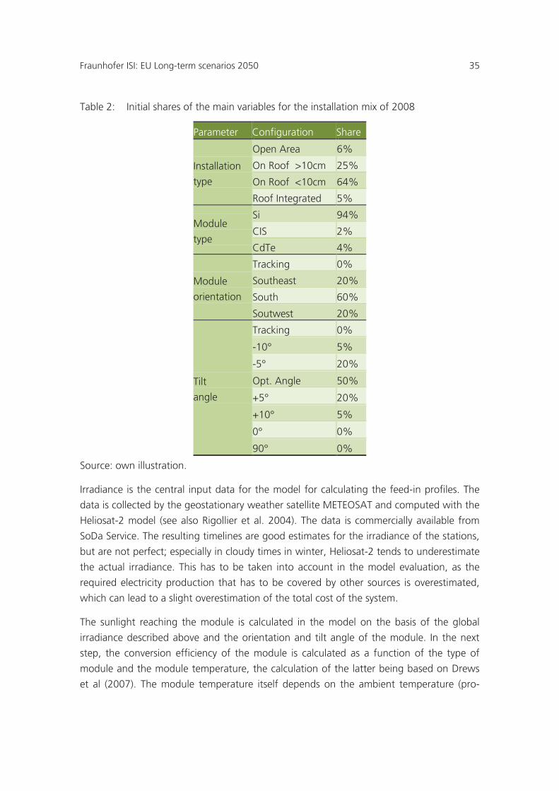
Table 2: Initial shares of the main variables for the installation mix of 2008 .............. 35
Table 3: Comparison between actual results of an existing PV plant of 1.32 MW capacity in Dresden and results of ISI-PV-Europe for the same site and plant size ......................................................................................... 38
Table 4: Comparison of data published by Eurostat and results of ISI-PV-Europe for the years 2006-2008 ................................................................... 39
Table 5: Weather input data for ISI-Wind-Europe ...................................................... 43
Table 6: Key characteristics of the wind turbines ....................................................... 44
Table 7: Comparison of data published by Eurostat and results of ISI-Wind-Europe for 2008 ............................................................................................ 47
Table 8: Assumptions on the characteristics of conventional power plants in PowerACE-Europe ....................................................................................... 51
Table 9: Assumptions on the characteristics of net transfer capacities in PowerACE-Europe ....................................................................................... 52
Table 10: Assumptions on the characteristics of electricity storage facilities in PowerACE-Europe ....................................................................................... 54
Table 11: New conventional generation capacity built in the scenarios ....................... 59
Table 12: Impact of the meteorological dataset on the required interconnector capacity ........................................................................................................ 85
Table 13: Impact of RES-E generation on the electricity system in 2050 (Scenario A) .................................................................................................. 88
Table 14: Data Sheet; Region: EU27 +2M; year: 2050 ................................................ 90
Table 15: Development of electricity demand in Scenario A ........................................ 91
Table 16: Development of electricity demand in Scenario B ........................................ 92
Table 17: Input prices for fuels and emission permits .................................................. 93
Table 18: Installed development of RES-E capacity (Scenario A) ............................... 93
Table 19: Development of RES-E capacity (Scenario B) ............................................. 94
Table 20: Quick fact sheet Scenario A ....................................................................... 105
Table 21: Quick fact sheet Scenario B ....................................................................... 106
Fraunhofer ISI: EU Long-term scenarios 2050 11
Glossary
(AA)-CAES (Advanced adiabatic) compressed air energy storage
CAPEX Capital expenditures
CCGT Combined cycle gas turbine
CCS Carbon capture and storage
CSP Concentrating solar power
GIS geographic information system
GT Gas turbine
H2 Hydrogen
HVDC High voltage direct current
NREAP National Renewable Energy Action Plan
NTC Net transfer capacity
O&M Operation and maintenance
PHES Pumped hydro electric storages
xii Fraunhofer ISI: EU Long-term scenarios 2050
1 Introduction
The reduction of greenhouse gas emissions is one of the central challenges for the energy
supply in Europe. The electricity sector plays an important role, since it accounts for most
of the European CO2 emissions. This study investigates concrete and realizable ways to-
wards a European electricity sector in line with the goal of keeping global warming below
2°C. It analyzes the development of the electricity sector in the EU 27, Norway and Swit-
zerland (EU27+2) up to the year 2050. Thereby the study focuses on a high diffusion of
renewable electricity generation in order to achieve ambitious greenhouse gas reduction
targets. Given this focus, the study analyzes the impacts of increased efficiency in electric-
ity consumption on the required infrastructure, the structure of the electricity supply and
the cost of the system. The study is carried out by the Fraunhofer Institute for Systems and
Innovation Research (ISI) for the German Federal Ministry for the Environment, Nature
Conservation and Nuclear Safety.
1.1 Approach
Analysing the electricity sector in Europe as a whole is a complex task. It requires data on
important parameters such as fuel prices, CO2 prices, stock of power plants, electricity
demand, renewable electricity generation and grid infrastructure. Since the balance be-
tween electricity supply and demand has to be maintained at all times, a detailed analysis
of the electricity sector requires a high temporal resolution. The central task of this project
is to set up an analytical framework which is suitable for the given task.
A first step to keep the analysis manageable is to set up scenarios defined by external pa-
rameters which are not modelled endogenously. Among these are electricity demand, fuel
prices, CO2 prices and the emission reduction path. Since the goal of this study is to show
how ambitious reductions in greenhouse gas emissions can be achieved with high pene-
tration of renewable electricity generation (RES-E), two scenarios are defined which
achieve a reduction in CO2 emissions to 5% of the 1990 emission levels. This setting is in
line with recent publications of the European Commission, in which the electricity sector
decreases its emissions to 1 to 7 % of the 1990 level (European Commission 2011b).
Since both scenarios assumme ambitious climate policies which require a decarbonisation
of the electricity sector, fuel prices and CO2 prices are equal in both scenarios. As the sec-
ond goal of this study is to show the impact of increased efforts on the structure of the
electricity supply and the cost of the system, the main difference between the scenario
parameters is the development of electricity demand which is approximately 530 TWh
higher in Scenario B “Moderate efficiency” than in Scenario A “High efficiency”. The de-
Fraunhofer ISI: EU Long-term scenarios 2050 13
velopment of electricity demand in both scenarios is based on existing studies. A more
detailed description of the selected input parameters is given in chapter 2.
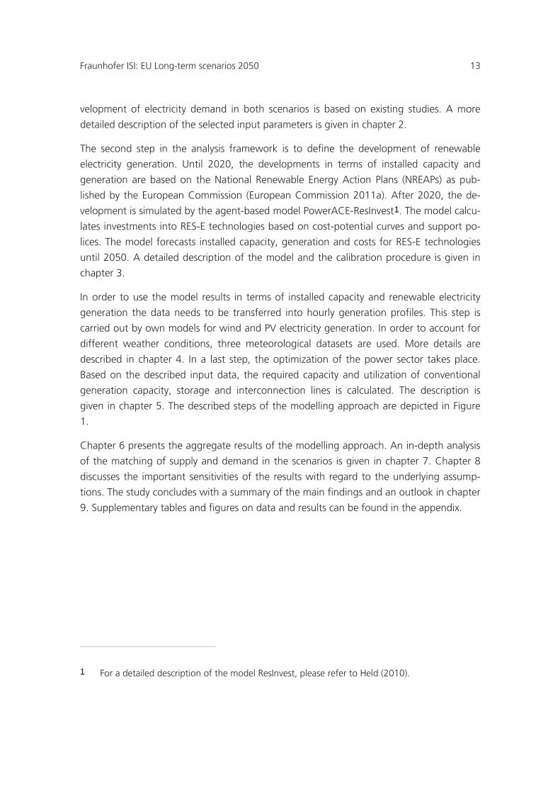
The second step in the analysis framework is to define the development of renewable
electricity generation. Until 2020, the developments in terms of installed capacity and
generation are based on the National Renewable Energy Action Plans (NREAPs) as pub-
lished by the European Commission (European Commission 2011a). After 2020, the de-
velopment is simulated by the agent-based model PowerACE-ResInvest1
3
. The model calcu-
lates investments into RES-E technologies based on cost-potential curves and support po-
lices. The model forecasts installed capacity, generation and costs for RES-E technologies
until 2050. A detailed description of the model and the calibration procedure is given in
chapter .
In order to use the model results in terms of installed capacity and renewable electricity
generation the data needs to be transferred into hourly generation profiles. This step is
carried out by own models for wind and PV electricity generation. In order to account for
different weather conditions, three meteorological datasets are used. More details are
described in chapter 4. In a last step, the optimization of the power sector takes place.
Based on the described input data, the required capacity and utilization of conventional
generation capacity, storage and interconnection lines is calculated. The description is
given in chapter 5. The described steps of the modelling approach are depicted in Figure
1.
Chapter 6 presents the aggregate results of the modelling approach. An in-depth analysis
of the matching of supply and demand in the scenarios is given in chapter 7. Chapter 8
discusses the important sensitivities of the results with regard to the underlying assump-
tions. The study concludes with a summary of the main findings and an outlook in chapter
9. Supplementary tables and figures on data and results can be found in the appendix.
1 For a detailed description of the model ResInvest, please refer to Held (2010).
xiv Fraunhofer ISI: EU Long-term scenarios 2050
Figure 1: Step-wise approach of the scenario modelling in this study
Source: own visualization.
2 Definition of exogenous input parameters
This chapter defines the main input parameters applied in the scenario analysis. Among
these are electricity demand, fuel prices, CO2 prices and the CO2 emissions levels.
2.1 Electricity demand
One central focus of this study is to show the impact of increased efficiency in electricity
consumption on the cost and infrastructure of electricity supply. However, the focus of
this study is not to analyze the development of electricity demand itself. Therefore, the
development of electricity demand is based on existing studies. The scenarios are selected
in order to represent one development with very ambitious reductions in electricity de-
mand and one development with a moderate development of electricity demand. Scenario
A “High efficiency” is based on scenario results of the project ADAM (Jochem & Schade
2009). The second Scenario B “Moderate efficiency” is based on the electricity demand of
Definition of external parameters• Hourly electricity
demand• Fuel prices• CO2 prices• Emission reduction
Development of RES-E
• Model: PowerACE-ResInvest
• Output: RES-E capacity
Step 2
Feed-in profiles for photovoltaic and wind powerModel:
ISI-Wind, ISI-PV• Output:
Hourly generation profiles
Optimization of the power sector• Model:
PowerACE-Europe (applying least cost optimization)• Output:
Capacities and dispatch of: conventional power plants, interconnectors, electricity storages
Step 4
Calibration
Step 3Step 1
Fraunhofer ISI: EU Long-term scenarios 2050 15
the TRANS-CSP study2
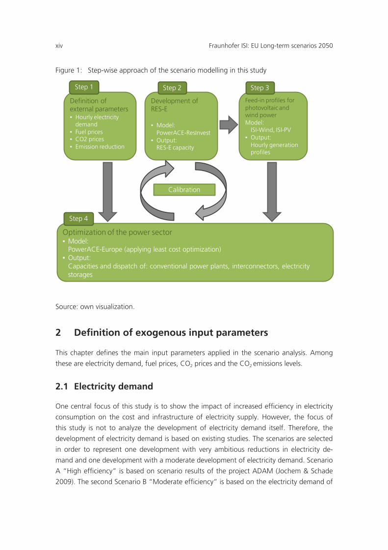
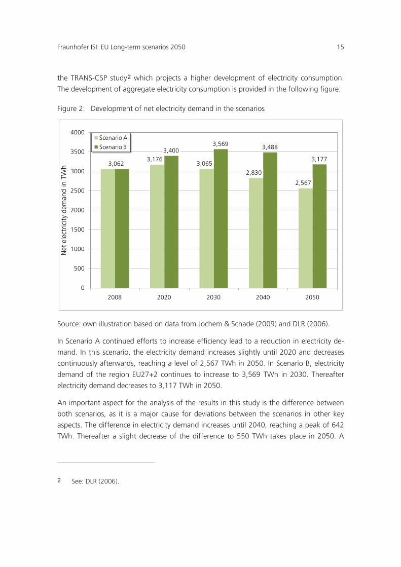
Figure 2: Development of net electricity demand in the scenarios
which projects a higher development of electricity consumption.
The development of aggregate electricity consumption is provided in the following figure.
Source: own illustration based on data from Jochem & Schade (2009) and DLR (2006).
In Scenario A continued efforts to increase efficiency lead to a reduction in electricity de-
mand. In this scenario, the electricity demand increases slightly until 2020 and decreases
continuously afterwards, reaching a level of 2,567 TWh in 2050. In Scenario B, electricity
demand of the region EU27+2 continues to increase to 3,569 TWh in 2030. Thereafter
electricity demand decreases to 3,117 TWh in 2050.
An important aspect for the analysis of the results in this study is the difference between
both scenarios, as it is a major cause for deviations between the scenarios in other key
aspects. The difference in electricity demand increases until 2040, reaching a peak of 642
TWh. Thereafter a slight decrease of the difference to 550 TWh takes place in 2050. A
2 See: DLR (2006).
3,0623,176
3,065
2,830
2,567
3,4003,569 3,488
3,177
0
500
1000
1500
2000
2500
3000
3500
4000
2008 2020 2030 2040 2050
Net
ele
ctric
ity d
eman
d in
TW
h
Scenario A
Scenario B
xvi Fraunhofer ISI: EU Long-term scenarios 2050
detailed table of the development of electricity demand in different countries is given in
the Appendix.
Net electricity demand by itself is not sufficient to determine the required net electricity
generation of the electricity sector. Since interconnector losses and storage losses are cal-
culated endogenously within the PowerACE-Europe model, only the losses in the national
grid have to be added to net electricity demand in order to provide an adequate model
input. An estimation of the grid losses can be found in the literature. Targosz (2008) esti-
mated the grid losses for EU-25 at 7.3%. Based on this estimate, grid losses for the region
EU27+2 are set at 7.5% in this study.
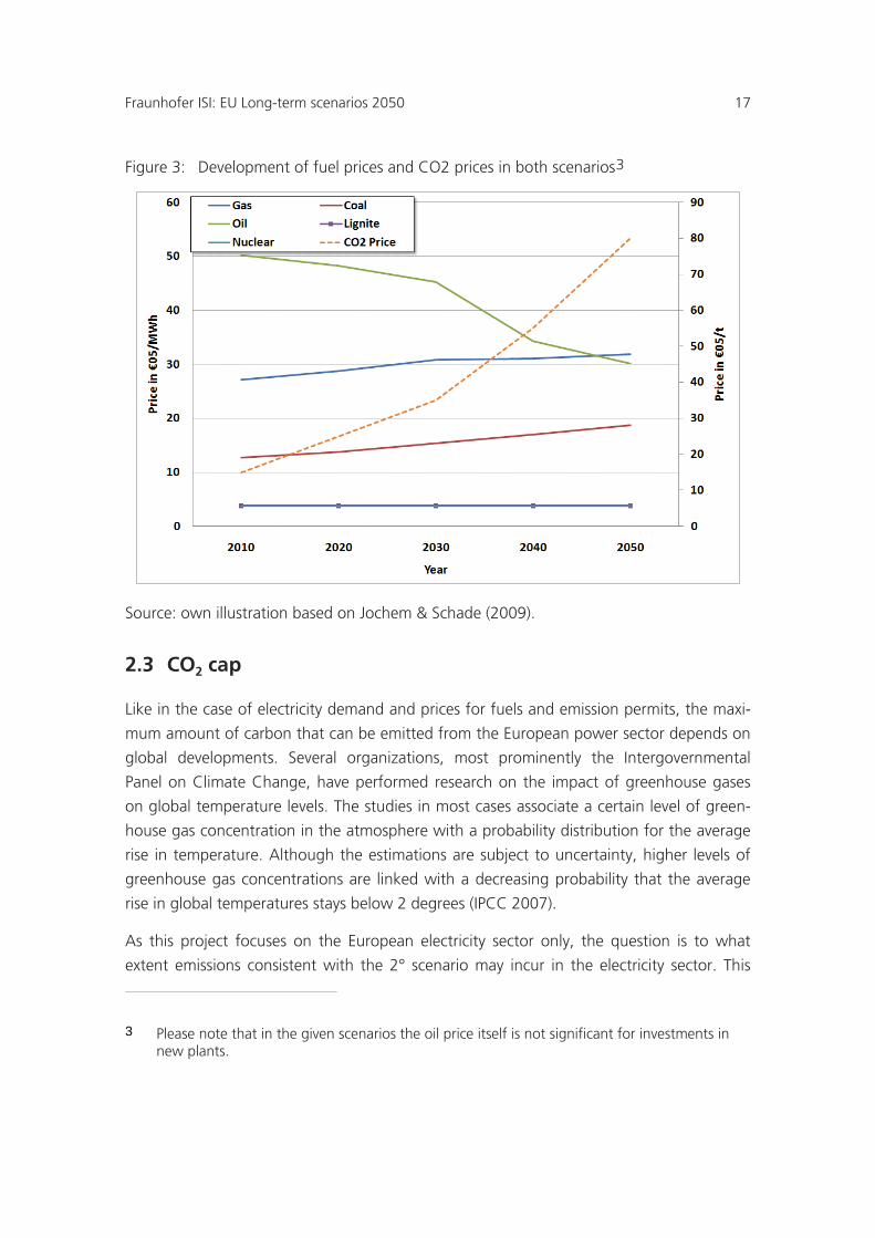
2.2 Fuel prices and CO2 prices
Another important input for the analysis is the development of fuel prices and CO2 prices.
In order to provide a sound dataset, the development of fuel prices and CO2 prices is also
based on the ADAM study. The development over time is shown in Figure 3. The fuel price
scenario corresponds to the same scenario in the ADAM project that also provides the
development of electricity demand of Scenario A. Furthermore, it is assumed that there is
no major change in the prices of lignite and nuclear fuel. The moderate development of
coal and gas prices and the decline in oil prices is surprising at first sight. This development
can be explained by the underlying assumption in the ADAM scenario that worldwide
efforts towards a strong reduction of greenhouse gas emission will take place, which has
a negative impact on the demand for fossil fuels. Nevertheless, the sensitivity of the results
towards changes in the assumed price developments is discussed in section 8.
Fraunhofer ISI: EU Long-term scenarios 2050 17
Figure 3: Development of fuel prices and CO2 prices in both scenarios3
Source: own illustration based on Jochem & Schade (2009).
2.3 CO2 cap
Like in the case of electricity demand and prices for fuels and emission permits, the maxi-
mum amount of carbon that can be emitted from the European power sector depends on
global developments. Several organizations, most prominently the Intergovernmental
Panel on Climate Change, have performed research on the impact of greenhouse gases
on global temperature levels. The studies in most cases associate a certain level of green-
house gas concentration in the atmosphere with a probability distribution for the average
rise in temperature. Although the estimations are subject to uncertainty, higher levels of
greenhouse gas concentrations are linked with a decreasing probability that the average
rise in global temperatures stays below 2 degrees (IPCC 2007).
As this project focuses on the European electricity sector only, the question is to what
extent emissions consistent with the 2° scenario may incur in the electricity sector. This
3 Please note that in the given scenarios the oil price itself is not significant for investments in new plants.
xviii Fraunhofer ISI: EU Long-term scenarios 2050
question is influenced not only by the technical potential of all sectors to decrease green-
house gas emissions, but also strongly depends on the costs associated with the reduc-
tion. In reality, many of the reductions could be triggered by the price of emission permits.
As all emitters will pay the same price, it is reasonable to assume that the marginal emit-
tent will set the price. Consequently, the question of which degree of decarbonisation of
the power sector is economical is thus linked to the developments of other sectors both in
Europe and the rest of the world.
An indication is given by studies that implicitly or explicitly dealt with this issue. In the
ADAM project, the electricity sector decreased its CO2 emissions by 80 to 100% (Jochem
& Schade 2009) between 2010 and 2050, depending on the applied model. The European
Commission recently published a study in which the electricity sector decreases its emis-
sions by 93 to 99 % compared to the 1990 level (European Commission 2011b). Other
recent studies, for example by the German Advisory Council on the Environment (SRU)
suggested that to reach the climate targets a full or almost full decarbonisation of the
electricity sector is feasible and is economically reasonable. (SRU 2010). This is based on
the fact that in other sectors, such as freight transport or aviation, reducing emissions to
very low levels is projected to be more costly than in the electricity sector.
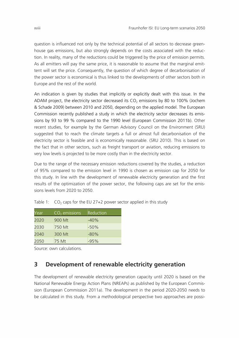
Due to the range of the necessary emission reductions covered by the studies, a reduction
of 95% compared to the emission level in 1990 is chosen as emission cap for 2050 for
this study. In line with the development of renewable electricity generation and the first
results of the optimization of the power sector, the following caps are set for the emis-
sions levels from 2020 to 2050.
Table 1: CO2 caps for the EU 27+2 power sector applied in this study
Source: own calculations.
3 Development of renewable electricity generation
The development of renewable electricity generation capacity until 2020 is based on the
National Renewable Energy Action Plans (NREAPs) as published by the European Commis-
sion (European Commission 2011a). The development in the period 2020-2050 needs to
be calculated in this study. From a methodological perspective two approaches are possi-
Year CO2 emissions Reduction
2020 900 Mt -40%
2030 750 Mt -50%
2040 300 Mt -80%
2050 75 Mt -95%
Fraunhofer ISI: EU Long-term scenarios 2050 19
ble: A least cost approach and a simulation approach. The first option is to include learn-
ing rates and RES-generatio potential data into a least cost optimization of the power sec-
tor. This option has two major disadvantages. First of all it can be questioned whether
such a pure least cost approach leads to a realitstic development of RES-E generation in
terms of regional distribution and development of the RES-E industry. Secondly, the re-
quired computational resources are beyond the resources that are available for this pro-
ject. Therefore, a simulation approach or the development of RES-generation is applied.
After 2020, the development is simulated by the model PowerACE-ResInvest (see also
Held, 2010) which contains detailed data on specific investments, learning rates and gen-
eration potential for renewable technologies in Europe. It includes 14 generation tech-
nologies and more than 5,000 generation potential classes. The development of genera-
tion capacity is based on a simulation of support schemes and maximum penetration lev-
els for wind and photovoltaic. The model also includes technological learning and a simu-
lation of the construction capacities for the different technologies. It has to be pointed out
that the simulated investments in renewable energy technologies differs from a pure least
cost approach for RES-E investments. The result is a rather distributed allocation of RES-E
plants over Europe.
3.1 Calibration and iteration procedure
A central task in this project is to provide an adequate diffusion scenario for renewable
electricity generation for the scenarios. The model PowerACE-ResInvest is used to provide
a consistent development of renewable electricity generation. In a first step, the model
calculates a RES-E diffusion, that is sufficient to reach the required emission reduction in
2050. The electricity generation calculated by PowerACE-ResInvest is used as input for the
electricity market model which is described in chapter 5. Basically, the model finds a least
cost mix of conventional generation, electricity storage and grid to a given scenario of
electricity demand and renewable generation under CO2 emission constraints. Based on
the results of both models the total cost of the electricity system are calculated. Thereafter
the calibration parameters of PowerACE-ResInvest are varied and a new dataset for the
renewable electricicty generation is calculated and fed into the electricity market model.
The total costs of the electricity system are calcuted and compared to the previous results.
After several iterations the PowerACE-ResInvest scenario is chosen that leads to the lowest
total system cost.
An adequate scenario for the development of RES-E generation needs to fulfil the follow-
ing criteria in order to ensure cost efficiency of the entire electricity system.
xx Fraunhofer ISI: EU Long-term scenarios 2050
1. The total amount of RES-E generation needs to be set adequately for the given
CO2 cap.
2. The RES-E generation mix in terms of technologies and regional distribution needs
to be set adequately.
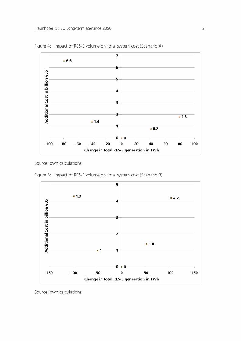
The appropriateness of the selected RES-generation scenarios with regard to the ade-
quate amount of renewable electricity generation in 2050 is tested in the following way.
The total renewable generation potential available in the power sector model in 2050 is
scaled in steps of 40 (Scenario A) or 50 TWh generation potential (Scenario B) and the
resulting total costs of the power sector are calculated. The change in renewable electric-
ity generation affects the cost of the remaining electricity system. The costs for additional
renewable generation4 are estimated5 Figure 3 and added to the total cost of the system.
and Figure 4 show the results of this analysis. It can be seen that neither an increase in
renewable generation nor a decrease in renewable generation leads to lower system costs.
In both cases the total system cost increase if the RES-E volume deviates from the selected
scenario value.
This result is caused by two competing effects. On the one hand, higher renewable elec-
tricity generation reduces the cost of the remaining supply infrastructures in a scenario
with fixed CO2 cap, since less conventional generation and interconnectors are required to
meet demand within the given CO2 cap. On the other hand, higher renewable generation
is accompanied by higher costs and the additional generation capacity needs to be cur-
tailed more often, when RES-E generation exceeds demand. This leads to situations in
which the share of the additional renewable generation that is actually utilized decreases
with growing installed capacity. A more detailed description of the discussed effects can
be found in chapter 8. In summary this sensitivity analysis shows that the amount of RES-E
generation is chosen adequately in the scenarios.
4 The renewable generation refers to the generation potential of the installed capacity and not the actual consumption, which differs due to curtailment and meteorological conditions.
5 Estimation is based on the marginal cost and slope of the underlying renewable cost potential curves.
Fraunhofer ISI: EU Long-term scenarios 2050 21
Figure 4: Impact of RES-E volume on total system cost (Scenario A)
Source: own calculations.
Figure 5: Impact of RES-E volume on total system cost (Scenario B)
Source: own calculations.
6.6
1.4
0
0.8
1.8
0
1
2
3
4
5
6
7
-100 -80 -60 -40 -20 0 20 40 60 80 100
Ad
dit
ion
al C
ost
in b
illio
n €
05
Change in total RES-E generation in TWh
4.3
1
0
1.4
4.2
0
1
2
3
4
5
-150 -100 -50 0 50 100 150
Ad
dit
ion
al C
ost
in b
illio
n €
05
Change in total RES-E generation in TWh
xxii Fraunhofer ISI: EU Long-term scenarios 2050
Besides the amount of renewable electricity generation, actual distribution of RES-E gen-
eration among technologies and regions influences the results strongly. In order to provide
better assessment of the question whether the obtained renewable electricity generation
is cost efficient, benchmark scenarios are calculated, applying different mixes of renew-
able electricity generation. Starting from the renewable generation projected by the
NREAPs in 2020, a renewable electricity generation mix in 2050 is developed which is
based on pure cost optimization of additional renewable generation. Such a scenario
could be the result of a harmonized international quota scheme without technological
differentiation, in which only the cheapest options for power generation from renewables
are exploited, without considering the consequential costs in the rest of the system. These
renewable generation portfolios are created for Scenarios A and B. Thereafter the total
cost of the electricity system is calculated. While the costs of renewable power generation
are lower in these scenarios, total system costs are higher. This is mainly caused by the
regional concentration of the low-cost renewable generation potentials. Among the
cheapest generation technologies is wind energy in northern Europe. Still, the regional
concentration of renewable generation requires extensive infrastructure, in terms of inter-
connectors and storage facilities. The more balanced approach in the results of
PowerACE-ResInvest also requires strong grid infrastructure for interconnectors to impor-
tant regions such as the UK and the Iberian Peninsula. Nevertheless, increasing RES-E con-
centration leads to increasing infrastructure costs which outweigh the savings in the cost
of renewable electricity generation in the tested scenarios. This is an interesting result for
the debate on the harmonization of renewable support schemes.
Having tested the adequacy of the amount and mix of RES-E generation it can be con-
cluded that the applied RES-E generation is sufficient in providing a low cost solution n the
given scenario setting. In addition, it provides a sound development of renewable invest-
ments which is crucial for the stable development of the renewable energy industry.
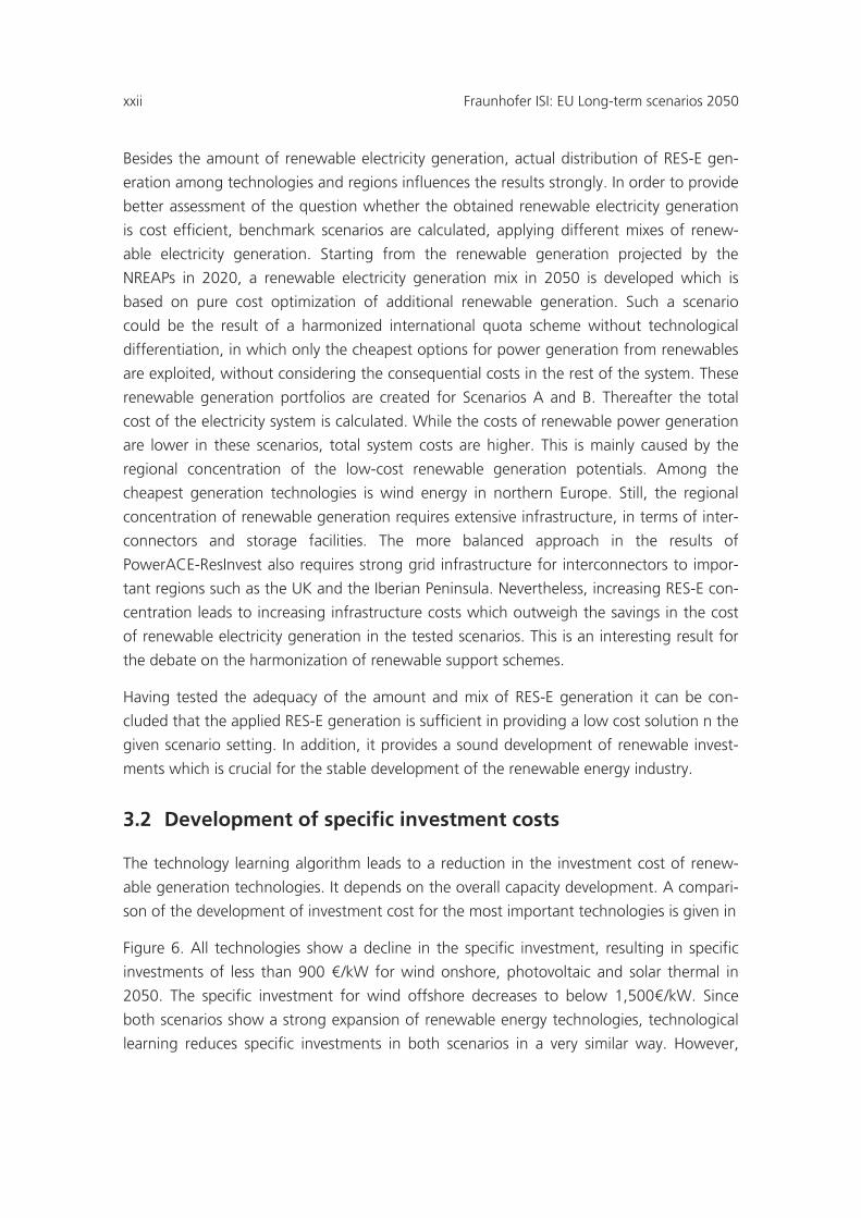
3.2 Development of specific investment costs
The technology learning algorithm leads to a reduction in the investment cost of renew-
able generation technologies. It depends on the overall capacity development. A compari-
son of the development of investment cost for the most important technologies is given in
Figure 6. All technologies show a decline in the specific investment, resulting in specific
investments of less than 900 €/kW for wind onshore, photovoltaic and solar thermal in
2050. The specific investment for wind offshore decreases to below 1,500€/kW. Since
both scenarios show a strong expansion of renewable energy technologies, technological
learning reduces specific investments in both scenarios in a very similar way. However,
Fraunhofer ISI: EU Long-term scenarios 2050 23
slight differences occur for wind offshore, where the stronger growth in Scenario B leads
to a slightly faster decrease in generation cost.
Figure 6: Development of specific investments for important RES-E Technologies
Source: own calculations.
3.3 Development of utilized renewable generation potential
The development of the utilized renewable electricity generation potential which is de-
fined as the possible output of the installed RES-E capacity, without taking curtailment
into account. The development in both scenarios is shown in Figure 7 and Figure 8. It is
important to note that these figures to not show actual utilization of renewable electricity
generation which can deviate because of changing meteorological datasets and curtail-
ment of renewable generation.
In both scenarios, wind energy and photovoltaic show a strong increase in generation
potential. The total generation potential of renewables grows to 2,781 TWh in Scenario A
und 3,432 TWh in Scenario B.
0
500
1,000
1,500
2,000
2,500
3,000
3,500
2010 2020 2030 2040 2050
Inve
stm
ent
in €
/kW
Photovoltaics Scenario A Solar thermal Scenario A
Wind offshore Scenario A Wind onshore Scenario A
Photovoltaics Scenario B Solar thermal Scenario B
Wind offshore Scenario B Wind onshore Scenario B
xxiv Fraunhofer ISI: EU Long-term scenarios 2050
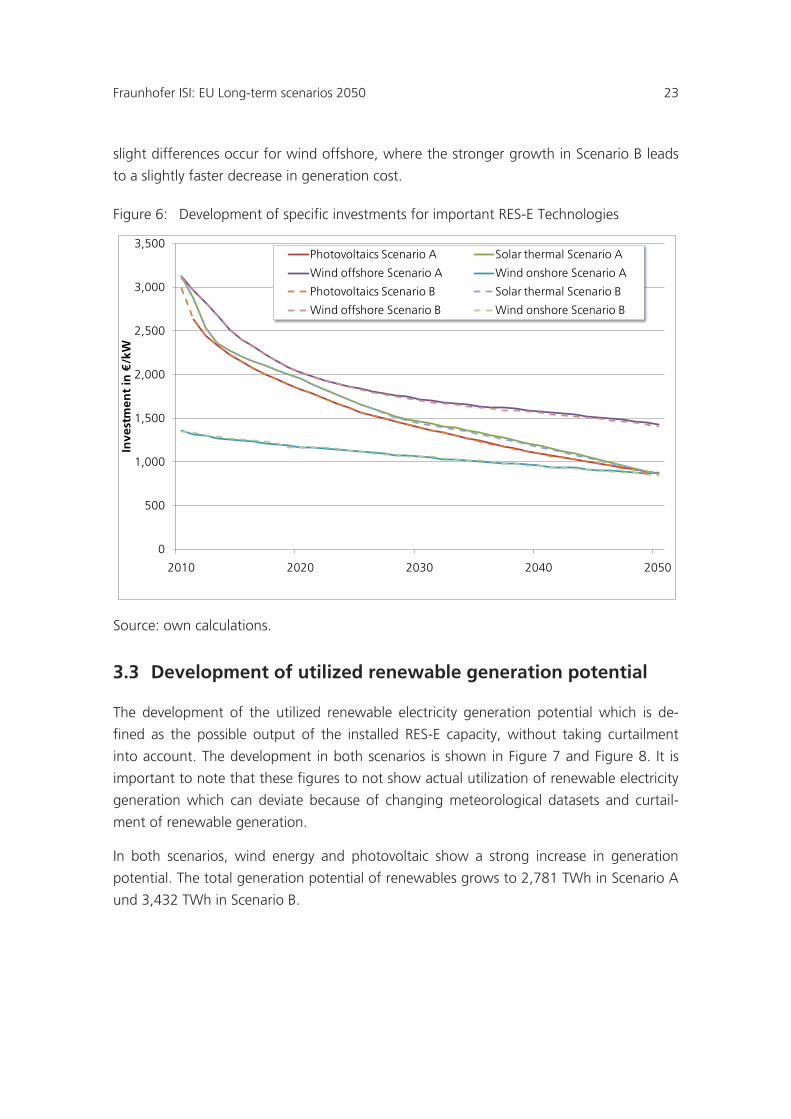
Figure 7: Generation potential of renewables in Scenario A
Source: own calculations.
In both scenarios, the strongest expansion in terms of additional generation potential can
be observed for wind power, both onshore and offshore, increasing in Scenario A to 882
TWh and 545 TWh, respectively. Consequently, wind accounts for approximately 51% of
the total generation potential in 2050. Besides wind power, PV shows the second strong-
est expansion with the generation potential growing by 9.1% per year on average be-
tween 2008 and 2050, thus totalling 333 TWh in 2050. Biomass and biogas increase only
moderately after 2020, as the major share of the domestic potential is already used by
2020. In sum, the two technologies can produce 306 TWh per year in 2050. A similar
development can be seen for hydropower. The largest part of the potential for large-scale
hydro is already exploited by 2020, whereas small-scale hydropower plants below 10 MW
capacity are installed moderately after 2020, especially in eastern Europe. Large-scale and
small-scale hydropower reach a generation potential of 487 and 81 TWh, respectively. The
generation potential of other renewable energy technologies grows steadily but rather
slowly, totalling 146 TWh in 2050. Power plants using biowaste and landfill or sewage gas
are mostly refurbished after 2020, but few new plants are installed. Concentrated solar
power (CSP) plays a certain role in some countries in southern Europe, especially in Spain,
whereas wave and tide power plants are installed in northern countries. Enhanced geo-
thermal technologies such as “hot dry rock” are not included in the model and the gen-
eration potential of conventional geothermal technologies is limited mostly to the Alpine
region. Therefore, the generation potential increases only to 12 TWh by 2050.
Fraunhofer ISI: EU Long-term scenarios 2050 25
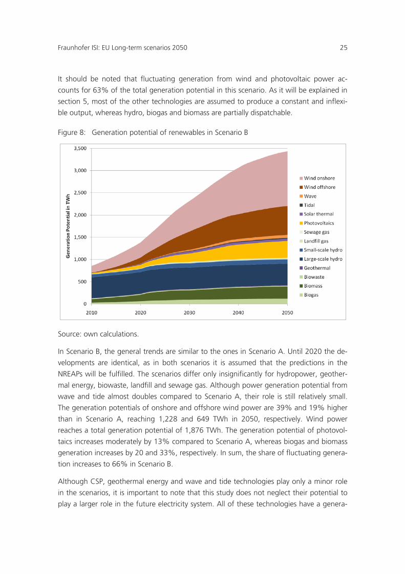
It should be noted that fluctuating generation from wind and photovoltaic power ac-
counts for 63% of the total generation potential in this scenario. As it will be explained in
section 5, most of the other technologies are assumed to produce a constant and inflexi-
ble output, whereas hydro, biogas and biomass are partially dispatchable.
Figure 8: Generation potential of renewables in Scenario B
Source: own calculations.
In Scenario B, the general trends are similar to the ones in Scenario A. Until 2020 the de-
velopments are identical, as in both scenarios it is assumed that the predictions in the
NREAPs will be fulfilled. The scenarios differ only insignificantly for hydropower, geother-
mal energy, biowaste, landfill and sewage gas. Although power generation potential from
wave and tide almost doubles compared to Scenario A, their role is still relatively small.
The generation potentials of onshore and offshore wind power are 39% and 19% higher
than in Scenario A, reaching 1,228 and 649 TWh in 2050, respectively. Wind power
reaches a total generation potential of 1,876 TWh. The generation potential of photovol-
taics increases moderately by 13% compared to Scenario A, whereas biogas and biomass
generation increases by 20 and 33%, respectively. In sum, the share of fluctuating genera-
tion increases to 66% in Scenario B.
Although CSP, geothermal energy and wave and tide technologies play only a minor role
in the scenarios, it is important to note that this study does not neglect their potential to
play a larger role in the future electricity system. All of these technologies have a genera-
xxvi Fraunhofer ISI: EU Long-term scenarios 2050
tion potential much larger than the one utilized in the scenarios presented here. Nonethe-
less, without technical breakthroughs, and at current learning rates, the technologies are
in many cases not competitive with other forms of renewable energies technologies. As
these breakthroughs cannot be anticipated by the model, increasing the shares of the
technologies would lead to higher costs of the scenarios.
3.4 Regional distribution of renewable electricity generation
The regional distribution of the installed capacity and generation is an important result of
the investment model and a central input for the modelling of the power system. As men-
tioned before, the renewable energy investment model uses cost-potential curves, techni-
cal parameters and restrictions and projected adaptations to the support systems to simu-
late the investments in renewable energy technologies.
As an example, the resulting capacities installed in 2050 for wind onshore and offshore as
calculated by the model are depicted in Figure 9 and Figure 10, whereas Figure 11 shows
the installed PV capacities. Wind power and PV are chosen as examples, since their impor-
tant role in electricity generation and their fluctuating nature act as a trigger for several
developments in the scenarios discussed later on. The maps for the other technologies and
for Scenario B can be found in the Appendix. Several conclusions can be drawn from the
figures.
First of all, the countries adjacent to the North- and Baltic Sea as well as Spain and Portu-
gal have high wind power capacities in absolute numbers. This is caused by favourable
wind regimes, in combination with attractive support schemes. In eastern and southern
Europe fewer wind parks are built by the model. Still, wind power is distributed all over
Europe and although it is utilized in some countries more than in others, it plays in impor-
tant role in the electricity generation of all countries.
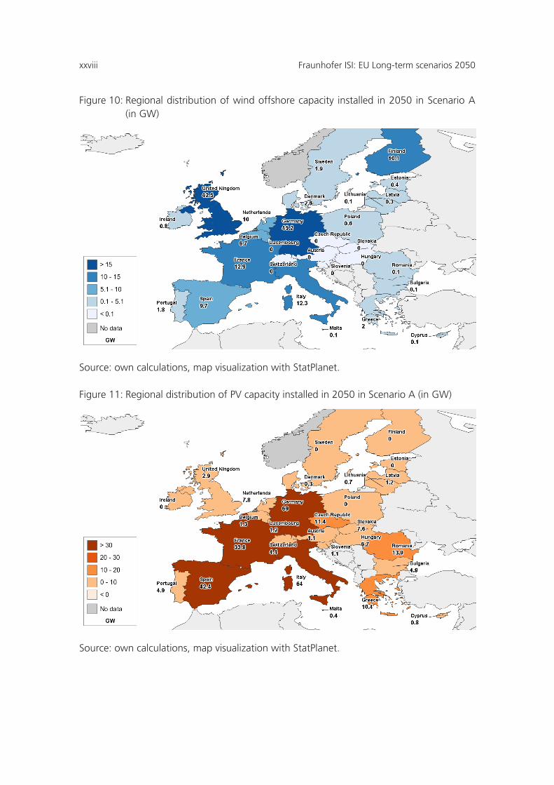
In the case of PV, the countries surrounding the Mediterranean Sea have a strong increase
in capacities. Furthermore, Germany shows a high figure in terms of installed capacity
because the potential of many other technologies is already exploited to a large degree by
2050 in the scenarios. Another reason is that the model assumes that Germany continues
to offer economically attractive feed-in tariffs for PV. It can been seen that the distribution
of PV over Europe is less homogeneous than in the case of wind, with several northern
countries having installed capacities below 500 MW.
Especially for wind power, it is also important to compare the installed capacity to the
maximum load occurring over the year. Several countries have an installed capacity that
exceeds their highest demand in any hour. In the Czech Republic, Estonia, Latvia, the
Netherlands, Poland, Portugal, Spain and the United Kingdom, the installed capacity of
Fraunhofer ISI: EU Long-term scenarios 2050 27
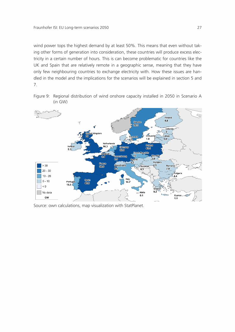
wind power tops the highest demand by at least 50%. This means that even without tak-
ing other forms of generation into consideration, these countries will produce excess elec-
tricity in a certain number of hours. This is can become problematic for countries like the
UK and Spain that are relatively remote in a geographic sense, meaning that they have
only few neighbouring countries to exchange electricity with. How these issues are han-
dled in the model and the implications for the scenarios will be explained in section 5 and
7.
Figure 9: Regional distribution of wind onshore capacity installed in 2050 in Scenario A (in GW)
Source: own calculations, map visualization with StatPlanet.
xxviii Fraunhofer ISI: EU Long-term scenarios 2050
Figure 10: Regional distribution of wind offshore capacity installed in 2050 in Scenario A (in GW)
Source: own calculations, map visualization with StatPlanet.
Figure 11: Regional distribution of PV capacity installed in 2050 in Scenario A (in GW)
Source: own calculations, map visualization with StatPlanet.
Fraunhofer ISI: EU Long-term scenarios 2050 29
4 Feed-in profiles for photovoltaic and wind power
The previous section describes how the model ResInvest is used to generate scenarios of
the development of renewables generation. The model provides annual timelines of in-
stalled capacities and generation for each technology and country. In order to utilize this
data in the electricity market model PowerACE-Europe, the annual data has to be trans-
formed into hourly feed-in profiles. For most technologies a constant production through-
out the year is assumed. Geothermal, wave, tide, landfill and sewage gas, as well as con-
centrating solar power (CSP) plants are assumed to produce a constant output throughout
the year. The impact of this simplification on the power system is rather small, as these
technologies play only a minor role in the scenarios and their aggregated output is in real-
ity relatively constant. The production from run-of-river hydropower is modelled on the
basis of monthly profiles where the data is available, which is the case for most countries
in the scenarios.
For the highly weather-dependent RES technologies wind and photovoltaic power, a more
detailed approach has to be chosen as the generation from these technologies fluctuates
strongly. For this study, real weather data of three years, 2006, 2007 and 2008 is used to
transform the annual data delivered by ResInvest into hourly profiles. The main advantage
of using actual weather data is that the correlation between the weather conditions in
different locations is included in the data.
The profiles for photovoltaic are based on processed satellite irradiation data of SoDa Ser-
vices6
The wind profiles are based on data of 3,097 weather measurement stations both on- and
offshore. The data was provided by Meteomedia AG and contains data on wind speed,
temperature and air pressure. The feed-in profiles are generated by modelling the output
of hypothetical wind farms at the measurement site by using the meteorological data,
roughness of the surrounding terrain and detailed information on the technical parame-
. The data points for this study are distributed with a distance of 0.5 times 0.5 de-
grees of longitude and latitude. In total, the data grid consists of 3,071 stations. To calcu-
late the profiles for PV, the irradiation data is fed into a model calculating the output of
PV modules. The photovoltaic conversion process is modelled on the basis of technical
parameters of the modules, including module and installation type, orientation and tem-
perature. As a simplification, it is assumed that the PV modules are distributed evenly
across locations in the respective country.
6 For information on the available data, please refer to: https://www.soda-is.com.
xxx Fraunhofer ISI: EU Long-term scenarios 2050
ters of the wind turbines. The wind turbine sites in use today are attributed to the nearest
measurement station and their aggregated production forms the feed-in profiles. Different
profiles are generated for onshore and offshore sites.
In the following section, the assumptions and methods applied in the process of generat-
ing the hourly profiles is described in greater detail, as it is a central task of the project and
the overall results of the scenario simulation depend very much on the premises used in
the modelling approach. It should be noted though that the description is rather specific
and not mandatory for understanding the chapters thereafter.
4.1 Profiles for photovoltaic
Photovoltaic (PV) systems transform solar light into electric energy. The amount of electric-
ity fed into the grid by a single module, a park or a country is determined by several vari-
ables, which are briefly introduced in the following.
Irradiance is the primary factor defining the generation of the module. The irradiance
reaching the solar panel depends primarily on the position of sun, clouds and the orienta-
tion of the module. Furthermore, soil reflectance (albedo) and shading of the module by
surrounding objects (like buildings and trees) play a role, although companies installing PV
modules try to minimize the effects of the latter by appropriately siting the modules. The
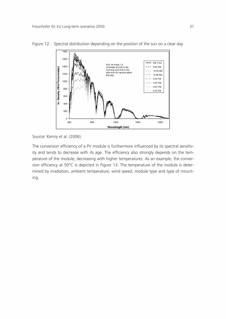
spectral distribution of sunlight is variable, as the wavelengths absorbed by the atmos-
phere depend on the position of the sun and the resulting optical path length through the
atmosphere described by air mass. As shown in Figure 12 especially short wavelengths are
blocked in times of high air mass and low position of the sun.
Fraunhofer ISI: EU Long-term scenarios 2050 31
Figure 12: Spectral distribution depending on the position of the sun on a clear day
Source: Kenny et al. (2006).
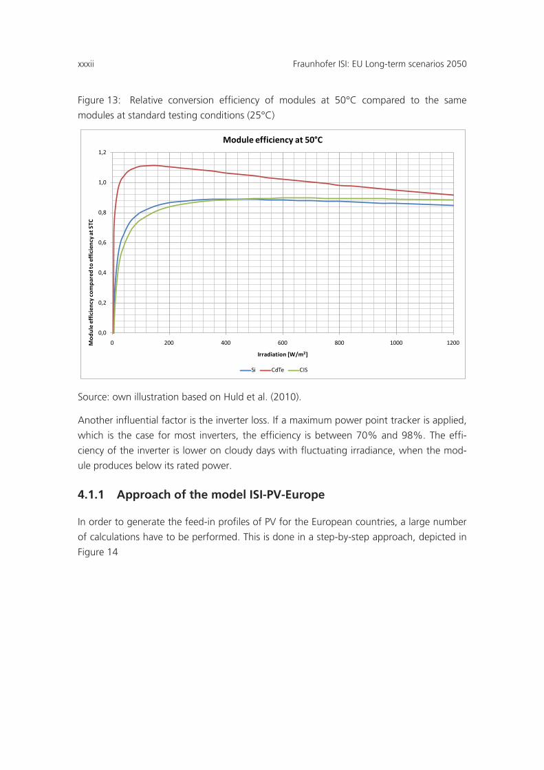
The conversion efficiency of a PV module is furthermore influenced by its spectral sensitiv-
ity and tends to decrease with its age. The efficiency also strongly depends on the tem-
perature of the module, decreasing with higher temperatures. As an example, the conver-
sion efficiency at 50°C is depicted in Figure 13. The temperature of the module is deter-
mined by irradiation, ambient temperature, wind speed, module type and type of mount-
ing.
xxxii Fraunhofer ISI: EU Long-term scenarios 2050
Figure 13: Relative conversion efficiency of modules at 50°C compared to the same
modules at standard testing conditions (25°C)
Source: own illustration based on Huld et al. (2010).
Another influential factor is the inverter loss. If a maximum power point tracker is applied,
which is the case for most inverters, the efficiency is between 70% and 98%. The effi-
ciency of the inverter is lower on cloudy days with fluctuating irradiance, when the mod-
ule produces below its rated power.
4.1.1 Approach of the model ISI-PV-Europe
In order to generate the feed-in profiles of PV for the European countries, a large number
of calculations have to be performed. This is done in a step-by-step approach, depicted in
Figure 14
0,0
0,2
0,4
0,6
0,8
1,0
1,2
0 200 400 600 800 1000 1200Mod
ule
effic
ienc
y co
mpa
red
to e
ffici
ency
at S
TC
Irradiation [W/m2]
Module efficiency at 50°C
Si CdTe CIS
Fraunhofer ISI: EU Long-term scenarios 2050 33
Figure 14: Simplified representation of the approach used in ISI-PV-Europe
Source: own illustration.
In the developed model ISI-PV-Europe, the countries are subdivided into regions, which
consist of one or more virtual stations. Figure 15 shows the distribution of the stations in
Europe. The stations are distributed with a distance of 0.5 times 0.5 degrees of longitude
and latitude. This implies that one station represents an area of less than 2,500 km². A
higher resolution would be possible, but would not significantly increase the accuracy of
the results at country level.
xxxiv Fraunhofer ISI: EU Long-term scenarios 2050
Figure 15: Distribution of data points used as PV stations in ISI-PV-Europe
Source: own illustration.
The next step is to define a representative mix of solar plants for the respective region.
Currently, the data basis for a realistic representation of the existing PV installation portfo-
lios is rather weak. Only for very few countries and regions is reliable data available on
which module types are utilized and how the modules are installed, e.g. on a roof or in an
empty field. No data is available on actual tilt angles and module orientation (i.e. azimuth).
In consequence, one representative set-up was defined for this project and used for all
stations until better data becomes available. The set-up chosen and shown in Table 4 is
based on existing literature. The configuration is constant in the scenarios over the years.
Fraunhofer ISI: EU Long-term scenarios 2050 35
Table 2: Initial shares of the main variables for the installation mix of 2008
Parameter Configuration Share
Installation
type
Open Area 6%
On Roof >10cm 25%
On Roof <10cm 64%
Roof Integrated 5%
Module
type
Si 94%
CIS 2%
CdTe 4%
Module
orientation
Tracking 0%
Southeast 20%
South 60%
Soutwest 20%
Tilt
angle
Tracking 0%
-10° 5%
-5° 20%
Opt. Angle 50%
+5° 20%
+10° 5%
0° 0%
90° 0%
Source: own illustration.
Irradiance is the central input data for the model for calculating the feed-in profiles. The
data is collected by the geostationary weather satellite METEOSAT and computed with the
Heliosat-2 model (see also Rigollier et al. 2004). The data is commercially available from
SoDa Service. The resulting timelines are good estimates for the irradiance of the stations,
but are not perfect; especially in cloudy times in winter, Heliosat-2 tends to underestimate
the actual irradiance. This has to be taken into account in the model evaluation, as the
required electricity production that has to be covered by other sources is overestimated,
which can lead to a slight overestimation of the total cost of the system.
The sunlight reaching the module is calculated in the model on the basis of the global
irradiance described above and the orientation and tilt angle of the module. In the next
step, the conversion efficiency of the module is calculated as a function of the type of
module and the module temperature, the calculation of the latter being based on Drews
et al (2007). The module temperature itself depends on the ambient temperature (pro-
xxxvi Fraunhofer ISI: EU Long-term scenarios 2050
vided by the same weather stations also used in the wind model), wind speeds and the
type of mounting, as a module directly on the roof tends to have higher temperatures
than one on a higher mounting structure).
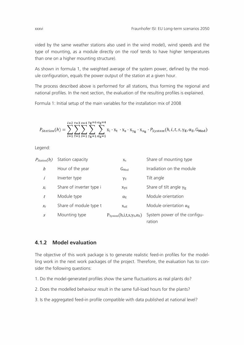
As shown in formula 1, the weighted average of the system power, defined by the mod-
ule configuration, equals the power output of the station at a given hour.
The process described above is performed for all stations, thus forming the regional and
national profiles. In the next section, the evaluation of the resulting profiles is explained.
Formula 1: Initial setup of the main variables for the installation mix of 2008
Legend:
PStation(h) Station capacity xs Share of mounting type
h Hour of the year GMod Irradiation on the module
i Inverter type γE Tilt angle
xi Share of inverter type i xγE Share of tilt angle γE
t Module type αE Module orientation
xt Share of module type t xαE Module orientation αE
s Mounting type PSystem(h,i,t,s,γE,αE) System power of the configu-
ration
4.1.2 Model evaluation
The objective of this work package is to generate realistic feed-in profiles for the model-
ling work in the next work packages of the project. Therefore, the evaluation has to con-
sider the following questions:
1. Do the model-generated profiles show the same fluctuations as real plants do?
2. Does the modelled behaviour result in the same full-load hours for the plants?
3. Is the aggregated feed-in profile compatible with data published at national level?
Fraunhofer ISI: EU Long-term scenarios 2050 37
This means that the model has to be evaluated using time series of PV plants for bench-
marking. Unfortunately, no data has been published on the aggregated behaviour of all
PV plants within a country for the years 2006-2008. For Germany, the cumulated hourly
feed-in profile is available, starting in July 2010. The data currently covers a time span too
short to be used for evaluation purposes.
For this reason, two PV plants in Dresden, Germany were used as benchmarks. The plants
consist of 6 polycrystalline modules of 220 W each and are installed in a field in a fixed
angle of 35%. Surrounding trees cast shadows on the field in some months, especially in
the early and late hours of the day. Data on the plants generation exist for February to
November 2008. The differences between the electricity generation of both plants are
insignificant.
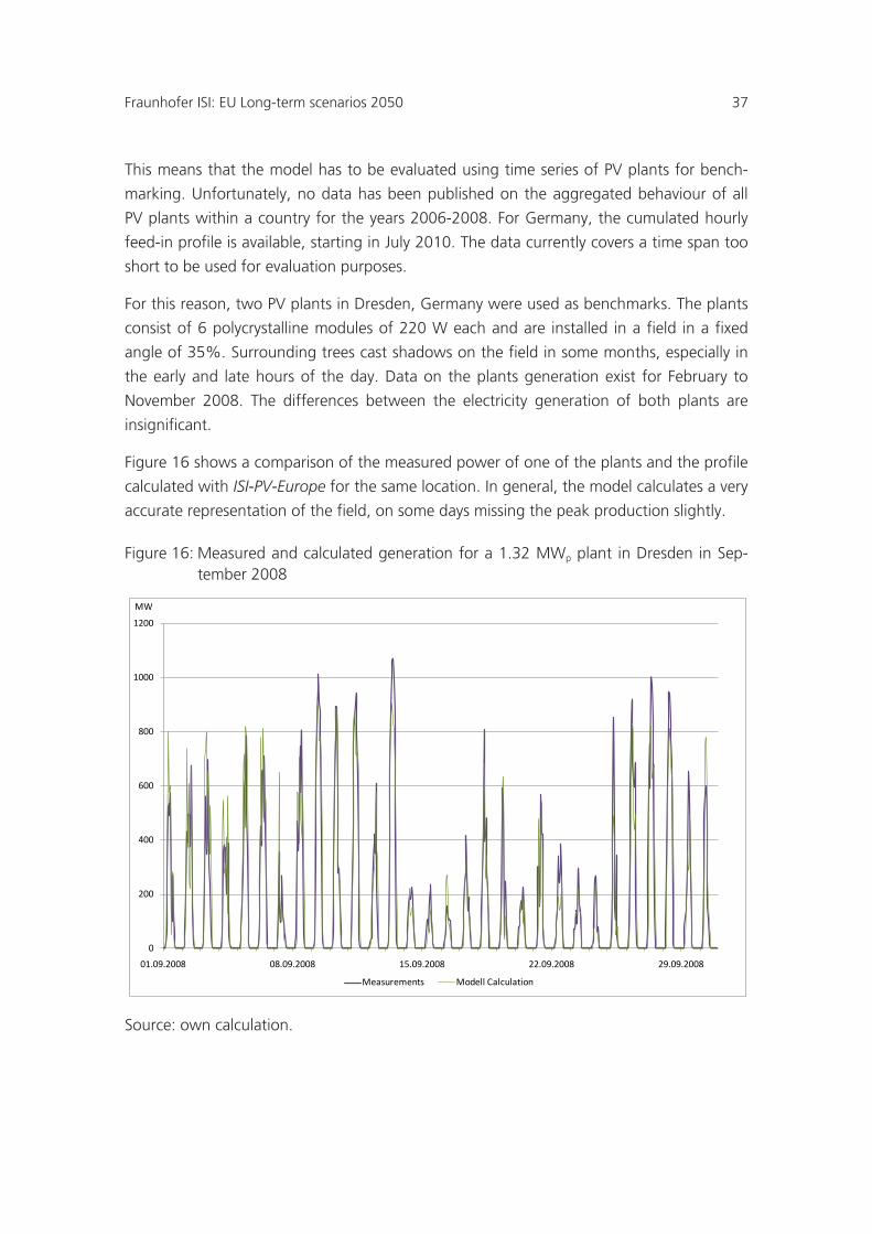
Figure 16 shows a comparison of the measured power of one of the plants and the profile
calculated with ISI-PV-Europe for the same location. In general, the model calculates a very
accurate representation of the field, on some days missing the peak production slightly.
Figure 16: Measured and calculated generation for a 1.32 MWp plant in Dresden in Sep-tember 2008
Source: own calculation.
0
200
400
600
800
1000
1200
01.09.2008 08.09.2008 15.09.2008 22.09.2008 29.09.2008
Measurements Modell Calculation
MW
xxxviii Fraunhofer ISI: EU Long-term scenarios 2050
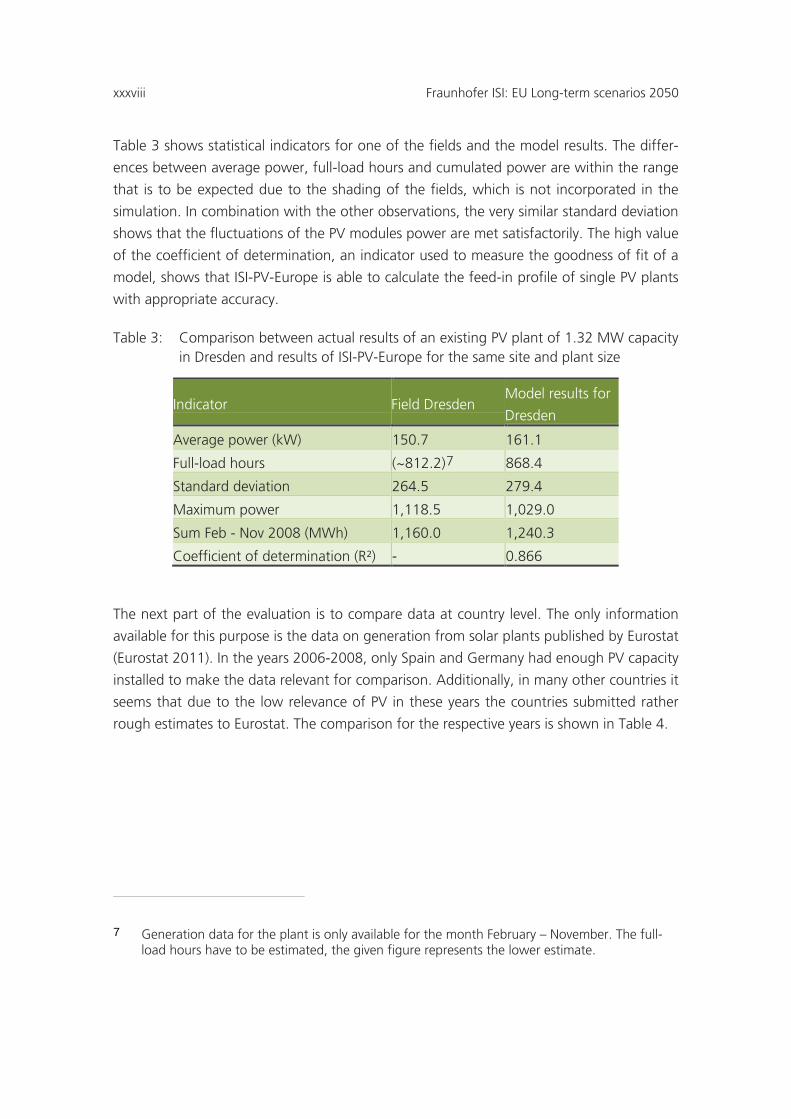
Table 3 shows statistical indicators for one of the fields and the model results. The differ-
ences between average power, full-load hours and cumulated power are within the range
that is to be expected due to the shading of the fields, which is not incorporated in the
simulation. In combination with the other observations, the very similar standard deviation
shows that the fluctuations of the PV modules power are met satisfactorily. The high value
of the coefficient of determination, an indicator used to measure the goodness of fit of a
model, shows that ISI-PV-Europe is able to calculate the feed-in profile of single PV plants
with appropriate accuracy.
Table 3: Comparison between actual results of an existing PV plant of 1.32 MW capacity in Dresden and results of ISI-PV-Europe for the same site and plant size
Indicator Field Dresden Model results for
Dresden
Average power (kW) 150.7 161.1
Full-load hours (~812.2)7 868.4
Standard deviation 264.5 279.4
Maximum power 1,118.5 1,029.0
Sum Feb - Nov 2008 (MWh) 1,160.0 1,240.3
Coefficient of determination (R²) - 0.866
The next part of the evaluation is to compare data at country level. The only information
available for this purpose is the data on generation from solar plants published by Eurostat
(Eurostat 2011). In the years 2006-2008, only Spain and Germany had enough PV capacity
installed to make the data relevant for comparison. Additionally, in many other countries it
seems that due to the low relevance of PV in these years the countries submitted rather
rough estimates to Eurostat. The comparison for the respective years is shown in Table 4.
7 Generation data for the plant is only available for the month February – November. The full-load hours have to be estimated, the given figure represents the lower estimate.
Fraunhofer ISI: EU Long-term scenarios 2050 39
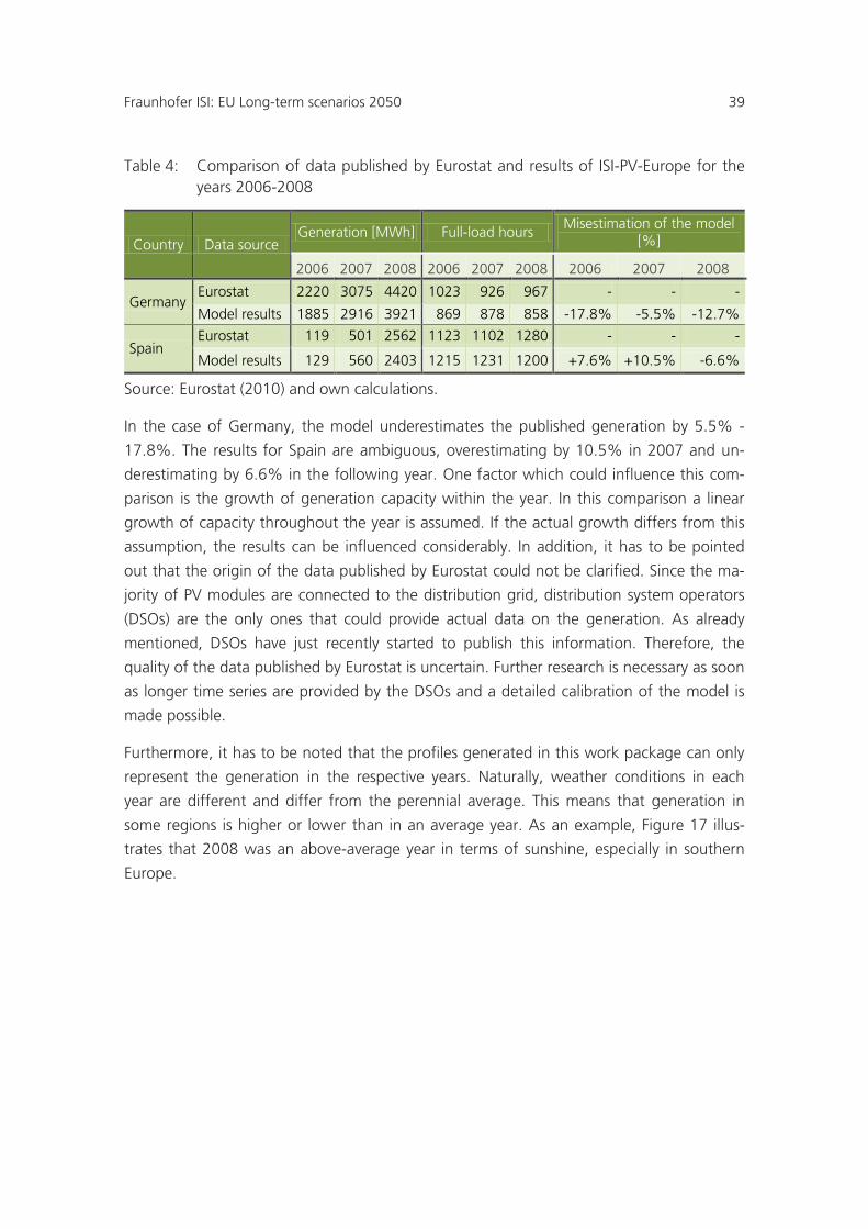
Table 4: Comparison of data published by Eurostat and results of ISI-PV-Europe for the years 2006-2008
Country Data source Generation [MWh] Full-load hours
Misestimation of the model [%]
2006 2007 2008 2006 2007 2008 2006 2007 2008
Germany Eurostat 2220 3075 4420 1023 926 967 - - -
Model results 1885 2916 3921 869 878 858 -17.8% -5.5% -12.7%
Spain Eurostat 119 501 2562 1123 1102 1280 - - -
Model results 129 560 2403 1215 1231 1200 +7.6% +10.5% -6.6%
Source: Eurostat (2010) and own calculations.
In the case of Germany, the model underestimates the published generation by 5.5% -
17.8%. The results for Spain are ambiguous, overestimating by 10.5% in 2007 and un-
derestimating by 6.6% in the following year. One factor which could influence this com-
parison is the growth of generation capacity within the year. In this comparison a linear
growth of capacity throughout the year is assumed. If the actual growth differs from this
assumption, the results can be influenced considerably. In addition, it has to be pointed
out that the origin of the data published by Eurostat could not be clarified. Since the ma-
jority of PV modules are connected to the distribution grid, distribution system operators
(DSOs) are the only ones that could provide actual data on the generation. As already
mentioned, DSOs have just recently started to publish this information. Therefore, the
quality of the data published by Eurostat is uncertain. Further research is necessary as soon
as longer time series are provided by the DSOs and a detailed calibration of the model is
made possible.
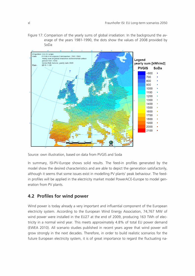
Furthermore, it has to be noted that the profiles generated in this work package can only
represent the generation in the respective years. Naturally, weather conditions in each
year are different and differ from the perennial average. This means that generation in
some regions is higher or lower than in an average year. As an example, Figure 17 illus-
trates that 2008 was an above-average year in terms of sunshine, especially in southern
Europe.
xl Fraunhofer ISI: EU Long-term scenarios 2050
Figure 17: Comparison of the yearly sums of global irradiation: In the background the av-erage of the years 1981-1990, the dots show the values of 2008 provided by SoDa
Source: own illustration, based on data from PVGIS and Soda
In summary, ISI-PV-Europe shows solid results. The feed-in profiles generated by the
model show the desired characteristics and are able to depict the generation satisfactorily,
although it seems that some issues exist in modelling PV plants’ peak behaviour. The feed-
in profiles will be applied in the electricity market model PowerACE-Europe to model gen-
eration from PV plants.
4.2 Profiles for wind power
Wind power is today already a very important and influential component of the European
electricity system. According to the European Wind Energy Association, 74,767 MW of
wind power were installed in the EU27 at the end of 2009, producing 163 TWh of elec-
tricity in a normal wind year. This meets approximately 4.8% of total EU power demand
(EWEA 2010). All scenario studies published in recent years agree that wind power will
grow strongly in the next decades. Therefore, in order to build realistic scenarios for the
future European electricity system, it is of great importance to regard the fluctuating na-
Fraunhofer ISI: EU Long-term scenarios 2050 41
ture of the generation from wind turbines. Consequently, one central objective of this
project is to generate accurate hourly wind power profiles for the EU27+2.
The model ISI-Wind-Europe developed in this project was used to transform weather data
into country wind power feed-in profiles. The approach of the model will be described in
the following.
4.2.1 Approach of the model ISI-Wind-Europe
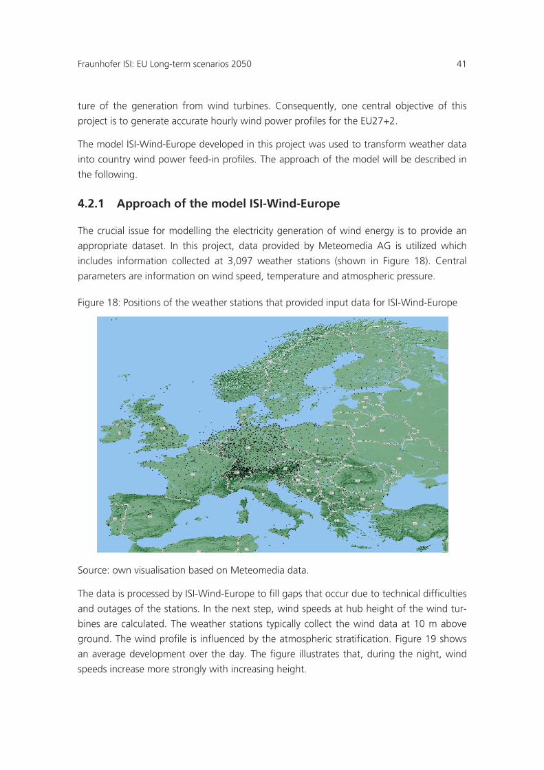
The crucial issue for modelling the electricity generation of wind energy is to provide an
appropriate dataset. In this project, data provided by Meteomedia AG is utilized which
includes information collected at 3,097 weather stations (shown in Figure 18). Central
parameters are information on wind speed, temperature and atmospheric pressure.
Figure 18: Positions of the weather stations that provided input data for ISI-Wind-Europe
Source: own visualisation based on Meteomedia data.
The data is processed by ISI-Wind-Europe to fill gaps that occur due to technical difficulties
and outages of the stations. In the next step, wind speeds at hub height of the wind tur-
bines are calculated. The weather stations typically collect the wind data at 10 m above
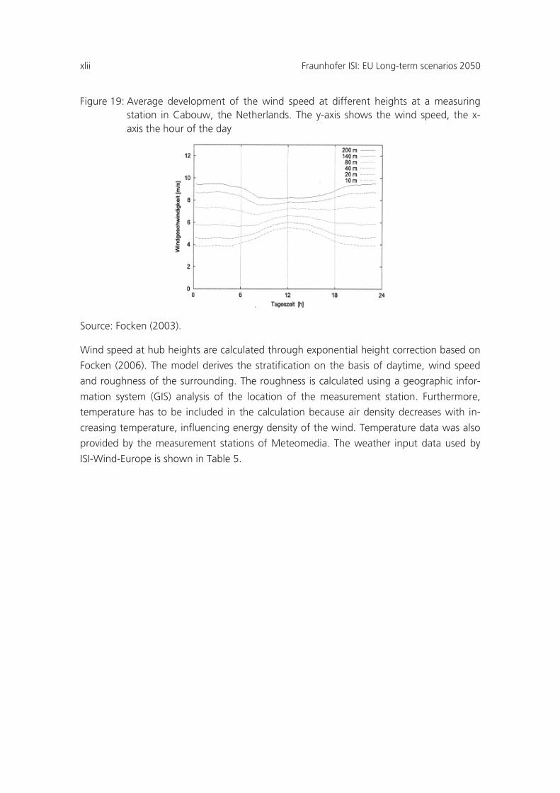
ground. The wind profile is influenced by the atmospheric stratification. Figure 19 shows
an average development over the day. The figure illustrates that, during the night, wind
speeds increase more strongly with increasing height.
xlii Fraunhofer ISI: EU Long-term scenarios 2050
Figure 19: Average development of the wind speed at different heights at a measuring station in Cabouw, the Netherlands. The y-axis shows the wind speed, the x-axis the hour of the day
Source: Focken (2003).
Wind speed at hub heights are calculated through exponential height correction based on
Focken (2006). The model derives the stratification on the basis of daytime, wind speed
and roughness of the surrounding. The roughness is calculated using a geographic infor-
mation system (GIS) analysis of the location of the measurement station. Furthermore,
temperature has to be included in the calculation because air density decreases with in-
creasing temperature, influencing energy density of the wind. Temperature data was also
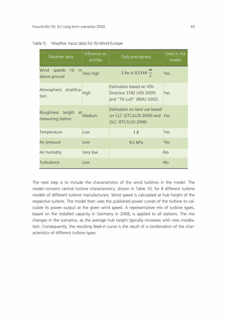
provided by the measurement stations of Meteomedia. The weather input data used by
ISI-Wind-Europe is shown in Table 5.
Fraunhofer ISI: EU Long-term scenarios 2050 43
Table 5: Weather input data for ISI-Wind-Europe
Weather data Influence on
profiles Data preciseness
Used in the
model
Wind speeds 10 m
above ground Very high 1 𝑘𝑛 ≅ 0,5144
𝑚𝑠
Yes
Atmospheric stratifica-
tion High
Estimation based on VDI-
Directive 3782 (VDI 2009)
and “TA Luft” (BMU 2002)
Yes
Roughness length at
measuring station Medium
Estimation on land use based
on CLC (ETC/LUSI 2009) and
GLC (ETC/LUSI 2006)
Yes
Temperature Low 1 𝐾 Yes
Air pressure Low 0,1 ℎ𝑃𝑎 Yes
Air humidity Very low - No
Turbulence Low - No
The next step is to include the characteristics of the wind turbines in the model. The
model contains central turbine characteristics, shown in Table 10, for 8 different turbine
models of different turbine manufacturers. Wind speed is calculated at hub height of the
respective turbine. The model then uses the published power curves of the turbine to cal-
culate its power output at the given wind speed. A representative mix of turbine types,
based on the installed capacity in Germany in 2008, is applied to all stations. The mix
changes in the scenarios, as the average hub height typically increases with new installa-
tion. Consequently, the resulting feed-in curve is the result of a combination of the char-
acteristics of different turbine types.
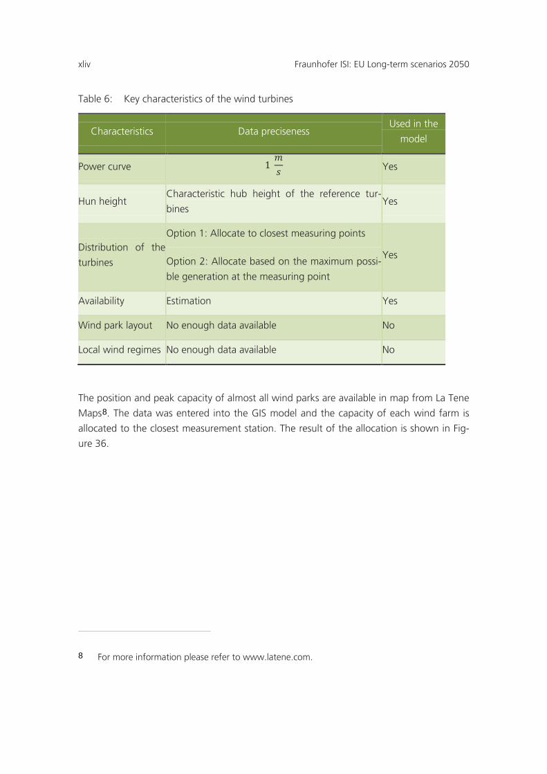
xliv Fraunhofer ISI: EU Long-term scenarios 2050
Table 6: Key characteristics of the wind turbines
Characteristics Data preciseness Used in the
model
Power curve 1 𝑚𝑠
Yes
Hun height Characteristic hub height of the reference tur-
bines Yes
Distribution of the
turbines
Option 1: Allocate to closest measuring points
Option 2: Allocate based on the maximum possi-
ble generation at the measuring point
Yes
Availability Estimation Yes
Wind park layout No enough data available No
Local wind regimes No enough data available No
The position and peak capacity of almost all wind parks are available in map from La Tene
Maps8
Fig-
ure 36
. The data was entered into the GIS model and the capacity of each wind farm is
allocated to the closest measurement station. The result of the allocation is shown in
.
8 For more information please refer to www.latene.com.
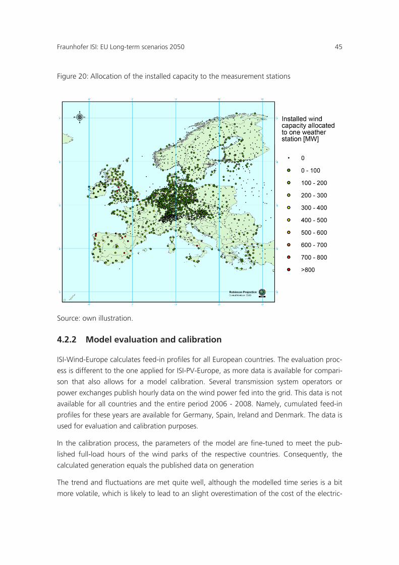
Fraunhofer ISI: EU Long-term scenarios 2050 45
Figure 20: Allocation of the installed capacity to the measurement stations
Source: own illustration.
4.2.2 Model evaluation and calibration
ISI-Wind-Europe calculates feed-in profiles for all European countries. The evaluation proc-
ess is different to the one applied for ISI-PV-Europe, as more data is available for compari-
son that also allows for a model calibration. Several transmission system operators or
power exchanges publish hourly data on the wind power fed into the grid. This data is not
available for all countries and the entire period 2006 - 2008. Namely, cumulated feed-in
profiles for these years are available for Germany, Spain, Ireland and Denmark. The data is
used for evaluation and calibration purposes.
In the calibration process, the parameters of the model are fine-tuned to meet the pub-
lished full-load hours of the wind parks of the respective countries. Consequently, the
calculated generation equals the published data on generation
The trend and fluctuations are met quite well, although the modelled time series is a bit
more volatile, which is likely to lead to an slight overestimation of the cost of the electric-
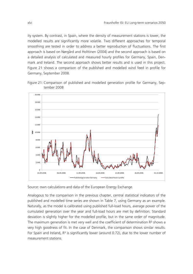
xlvi Fraunhofer ISI: EU Long-term scenarios 2050
ity system. By contrast, in Spain, where the density of measurement stations is lower, the
modelled results are significantly more volatile. Two different approaches for temporal
smoothing are tested in order to address a better reproduction of fluctuations. The first
approach is based on Nørgård and Holttinen (2004) and the second approach is based on
a detailed analysis of calculated and measured hourly profiles for Germany, Spain, Den-
mark and Ireland. The second approach shows better results and is used in this project.
Figure 21 shows a comparison of the published and modelled wind feed in profile for
Germany, September 2008.
Figure 21: Comparison of published and modelled generation profile for Germany, Sep-tember 2008
Source: own calculations and data of the European Energy Exchange.
Analogous to the comparison in the previous chapter, central statistical indicators of the
published and modelled time series are shown in Table 7, using Germany as an example.
Naturally, as the model is calibrated using published full-load hours, average power of the
cumulated generation over the year and full-load hours are met by definition. Standard
deviation is slightly higher for the modelled profile, but in the same order of magnitude.
The maximum generation is met very well and the coefficient of determination R² shows a
very high goodness of fit. In the case of Denmark, the comparison shows similar results.
For Spain and Ireland, R² is significantly lower (around 0.72), due to the lower number of
measurement stations.
0
2.000
4.000
6.000
8.000
10.000
12.000
14.000
16.000
18.000
20.000
01.09.2008 06.09.2008 11.09.2008 16.09.2008 21.09.2008 26.09.2008 01.10.2008
MW
Published generation Germany Calculated feed-in profile
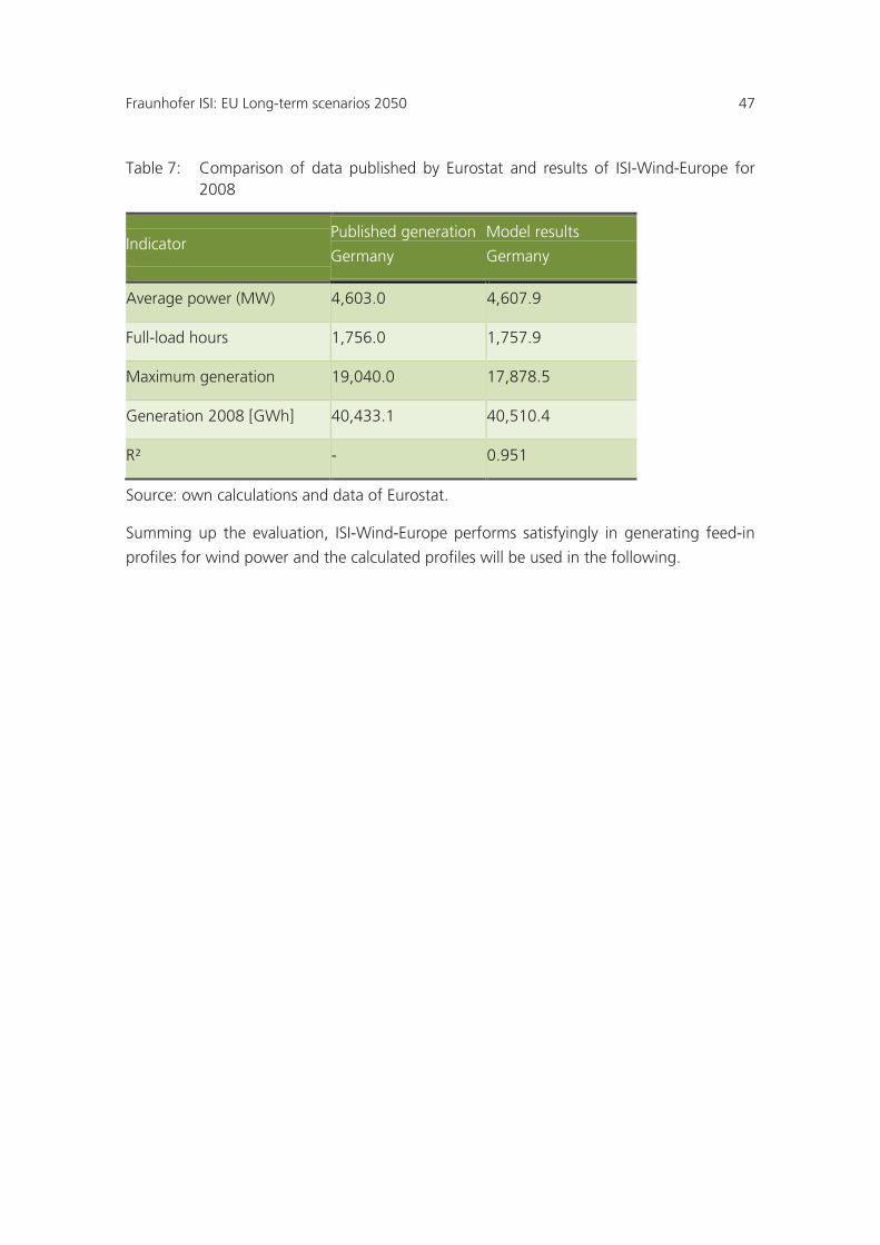
Fraunhofer ISI: EU Long-term scenarios 2050 47
Table 7: Comparison of data published by Eurostat and results of ISI-Wind-Europe for 2008
Indicator Published generation
Germany
Model results
Germany
Average power (MW) 4,603.0 4,607.9
Full-load hours 1,756.0 1,757.9
Maximum generation 19,040.0 17,878.5
Generation 2008 [GWh] 40,433.1 40,510.4
R² - 0.951
Source: own calculations and data of Eurostat.
Summing up the evaluation, ISI-Wind-Europe performs satisfyingly in generating feed-in
profiles for wind power and the calculated profiles will be used in the following.
xlviii Fraunhofer ISI: EU Long-term scenarios 2050
5 Optimization of the power sector
The steps described in the previous section add up to an aggregated description of the
power generation from renewable energies, including installed capacities, generation and
hourly load profiles. In the next step, the remaining parts of the power sector are opti-
mized in a least cost approach. The overarching question is, what technologies have to be
installed to secure that electricity demand is met at all hours of the analyzed years? To
account for the variability of generation from weather-dependent RES technologies, the
optimization is performed for the meteorological years 2006, 2007 and 2008.
In general, three types of technological options are incorporated in the optimization proc-
ess: conventional electricity generation technologies, interconnector lines between the
countries and electricity storage facilities. As already mentioned, these technologies will be
referred to as complementary technologies in the following, as their role is mainly to bal-
ance the fluctuating generation from renewable energies. In PowerACE-Europe, the opti-
mal mix of complementary technologies to a given renewable generation is calculated
using linear optimization. The problem to be solved and the applied constraints are ex-
plained in the following.
5.1 Optimization problem
The objective of the optimizer is to minimize the costs for meeting demand in all three
meteorological years. The costs taken into account are capital and operating expenditures
of all complementary technologies, including capital costs for investments, operation and
maintenance, fuels and the costs of carbon credits to be acquired for emissions. Conse-
quently, the cost function consists of two components: fixed costs occurring if the opti-
mizer decides to “build” one MW of capacity of a certain technology and a variable part,
depending on the utilization of the technology. The capital costs are calculated as annuity
in order to express the costs attributed to one year, as the model finds the least costs op-
tion for each year detached from other years.
The costs for transmission capacities are calculated based on the distance between the
weighted centres of demand for each country. The price of carbon credits is incorporated
as part of the variable costs of power plants. The costs assumptions for conventional
power generation are depicted in section 5.2.
The optimization is subject to several restrictions, the most important ones are explained
in the following.
1. Demand has to be met at all hours for each country, i.e. supply and consumption have
to be equal More precisely, this means that the sum of the power generation from both
Fraunhofer ISI: EU Long-term scenarios 2050 49
renewable and conventional plants, the output of storage facilities and electricity imported
from neighbouring countries, less the electricity consumed in the loading process of stor-
age facilities, electricity exported to other countries and the curtailment of renewable en-
ergy has to equal demand at every hour in every country. In this restriction both demand
and generation of most renewable technologies are fixed for each hour. The generation
from other technologies, such as conventional plants can be adjusted in the search for a
least cost option.
2. In a rather trivial restriction, the output of each power plant cannot be larger than its
installed capacity and each connector cannot transport power more than its transmission
capacity.
3. Storage plants can only operate within their technical limits. The filling level of the res-
ervoir or compressed air tank has to be between zero and its maximum. Pumping water
into the reservoirs, compressing air in compressed air energy storage facilities (CAES) and
electricity production from these facilities are restricted by the installed capacities.
4. Furthermore, the partially flexible generation of electricity from biomass, biogas and
hydro plants equipped with storage has to be taken into account. In the scenarios, 75%
of the power generation from biomass and biogas is assumed to be flexible. The FLH of
4,500 to 6,000 has to be met though, meaning that the flexibility is restricted. This also
applies to storage hydro plants, for which capacity and generation data is included in the
model for countries where these plants play a major role. The installed capacity and gen-
eration of these plants is kept at values for 2008 throughout the scenarios.
5. The total amount of C02 emissions is limited at a certain level for each year, decreasing
over time and reaching a 95% reduction compared to 1990 levels in the year 2050.
6. The availability of power plants is set at 95%.
Besides these main restrictions, several other aspects have to be incorporated, such as
losses occurring in power transmission or storage facilities and the integration of already
existing power plants and transmission capacities.
The resulting linear problem is solved for all scenario years and for all weather years using
a commercial solver programme. The results are stored in databases allowing access to the
information in aggregated or very detailed form.
In a first step, the optimal mix of complementary technologies is calculated for each year
without the influence of previous or following years. Afterwards a reasonable mix be-
tween renewable energies and complementary technologies is calculated, through multi-
ple model iterations of both ResInvest and PowerACE-Europe described in chapter 3. The
l Fraunhofer ISI: EU Long-term scenarios 2050
resulting scenario is the basis for a final iteration, in which the results in terms of installed
capacities (conventional plants, storages, interconnectors) from previous years are taken
into account in the following years. The result is a consistent scenario robust for all three
weather years in 2020, 2030, 2040 and 2050.
In the following the technical assumptions applied in the scenarios are presented.
5.2 Technological assumptions
As already mentioned before, the model uses conventional power plants, storage facilities
and grid expansions as complementary technologies to integrate renewable energies and
match demand and supply. The assumptions used in both scenarios will be explained in
the following.
5.2.1 Conventional power plants
The existing power plant park as of 2008 is included in the model in high detail, using
Platts’ World Electric Power Plant (WEPP) as data source9
Table 8
. The individual plants have to be
aggregated into groups to some extent to keep calculation time low. For the plants to be
installed in the future, only hard coal power plants and gas power plants, both as regular
gas turbines (GT) and combined cycle gas turbines (CCGT) are taken into consideration.
The technical assumptions are shown in .
9 For details on the database, please refer to: http://www.platts.com/Products/worldelectricpowerplantsdatabase
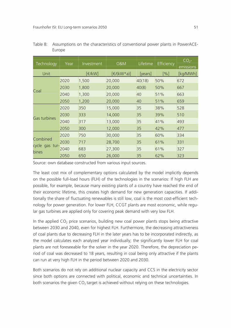
Fraunhofer ISI: EU Long-term scenarios 2050 51
Table 8: Assumptions on the characteristics of conventional power plants in PowerACE-Europe
Technology Year Investment O&M Lifetime Efficiency CO2-
emissions
Unit
[€/kW] [€/(kW*a)] [years] [%] [kg/MWh]
Coal
2020 1,500 20,000 40(18) 50% 672
2030 1,800 20,000 40(8) 50% 667
2040 1,300 20,000 40 51% 663
2050 1,200 20,000 40 51% 659
Gas turbines
2020 350 15,000 35 38% 528
2030 333 14,000 35 39% 510
2040 317 13,000 35 41% 493
2050 300 12,000 35 42% 477
Combined
cycle gas tur-
bines
2020 750 30,000 35 60% 334
2030 717 28,700 35 61% 331
2040 683 27,300 35 61% 327
2050 650 26,000 35 62% 323
Source: own database constructed from various input sources.
The least cost mix of complementary options calculated by the model implicitly depends
on the possible full-load hours (FLH) of the technologies in the scenarios: If high FLH are
possible, for example, because many existing plants of a country have reached the end of
their economic lifetime, this creates high demand for new generation capacities. If addi-
tionally the share of fluctuating renewables is still low, coal is the most cost-efficient tech-
nology for power generation. For lower FLH, CCGT plants are most economic, while regu-
lar gas turbines are applied only for covering peak demand with very low FLH.
In the applied CO2 price scenarios, building new coal power plants stops being attractive
between 2030 and 2040, even for highest FLH. Furthermore, the decreasing attractiveness
of coal plants due to decreasing FLH in the later years has to be incorporated indirectly, as
the model calculates each analyzed year individually; the significantly lower FLH for coal
plants are not foreseeable for the solver in the year 2020. Therefore, the depreciation pe-
riod of coal was decreased to 18 years, resulting in coal being only attractive if the plants
can run at very high FLH in the period between 2020 and 2030.
Both scenarios do not rely on additional nuclear capacity and CCS in the electricity sector
since both options are connected with political, economic and technical uncertainties. In
both scenarios the given CO2 target is achieved without relying on these technologies.
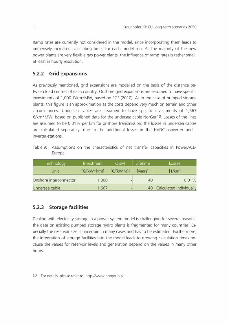
lii Fraunhofer ISI: EU Long-term scenarios 2050
Ramp rates are currently not considered in the model, since incorporating them leads to
immensely increased calculating times for each model run. As the majority of the new
power plants are very flexible gas power plants, the influence of ramp rates is rather small,
at least in hourly resolution.
5.2.2 Grid expansions
As previously mentioned, grid expansions are modelled on the basis of the distance be-
tween load centres of each country. Onshore grid expansions are assumed to have specific
investments of 1,000 €/km*MW, based on ECF (2010). As in the case of pumped storage
plants, this figure is an approximation as the costs depend very much on terrain and other
circumstances. Undersea cables are assumed to have specific investments of 1,667
€/km*MW, based on published data for the undersea cable NorGer10
Table 9: Assumptions on the characteristics of net transfer capacities in PowerACE-Europe
. Losses of the lines
are assumed to be 0.01% per km for onshore transmission; the losses in undersea cables
are calculated separately, due to the additional losses in the HVDC-converter and -
inverter-stations.
Technology Investment O&M Lifetime Losses
Unit [€/(kW*km)] [€/(kW*a)] [years] [1/km]
Onshore interconnector 1,000 - 40 0.01%
Undersea cable 1,667 - 40 Calculated individually
5.2.3 Storage facilities
Dealing with electricity storage in a power system model is challenging for several reasons:
the data on existing pumped storage hydro plants is fragmented for many countries. Es-
pecially the reservoir size is uncertain in many cases and has to be estimated. Furthermore,
the integration of storage facilities into the model leads to growing calculation times be-
cause the values for reservoir levels and generation depend on the values in many other
hours.
10 For details, please refer to: http://www.norger.biz/
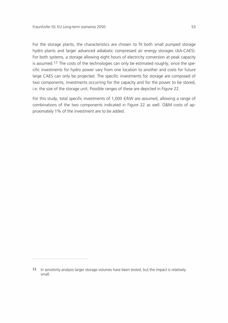
Fraunhofer ISI: EU Long-term scenarios 2050 53
For the storage plants, the characteristics are chosen to fit both small pumped storage
hydro plants and larger advanced adiabatic compressed air energy storages (AA-CAES).
For both systems, a storage allowing eight hours of electricity conversion at peak capacity
is assumed.11
Figure 22
The costs of the technologies can only be estimated roughly, since the spe-
cific investments for hydro power vary from one location to another and costs for future
large CAES can only be projected. The specific investments for storage are composed of
two components, investments occurring for the capacity and for the power to be stored,
i.e. the size of the storage unit. Possible ranges of these are depicted in .
For this study, total specific investments of 1,000 €/kW are assumed, allowing a range of
combinations of the two components indicated in Figure 22 as well. O&M costs of ap-
proximately 1% of the investment are to be added.
11 In sensitivity analysis larger storage volumes have been tested, but the impact is relatively small.
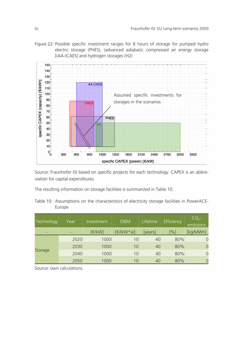
liv Fraunhofer ISI: EU Long-term scenarios 2050
Figure 22: Possible specific investment ranges for 8 hours of storage for pumped hydro electric storage (PHES), (advanced adiabatic compressed air energy storage [(AA-)CAES] and hydrogen storages (H2)
Source: Fraunhofer ISI based on specific projects for each technology. CAPEX is an abbre-
viation for capital expenditures.
The resulting information on storage facilities is summarized in Table 10.
Table 10: Assumptions on the characteristics of electricity storage facilities in PowerACE-Europe
Technology Year Investment O&M Lifetime Efficiency CO2-
emissions
- - [€/kW] [€/(kW*a)] [years] [%] [kg/MWh]
Storage
2020 1000 10 40 80% 0
2030 1000 10 40 80% 0
2040 1000 10 40 80% 0
2050 1000 10 40 80% 0
Source: own calculations.
Assumed specific investments for
storages in the scenarios
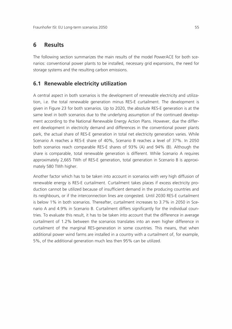
Fraunhofer ISI: EU Long-term scenarios 2050 55
6 Results
The following section summarizes the main results of the model PowerACE for both sce-
narios: conventional power plants to be installed, necessary grid expansions, the need for
storage systems and the resulting carbon emissions.
6.1 Renewable electricity utilization
A central aspect in both scenarios is the development of renewable electricity and utiliza-
tion, i.e. the total renewable generation minus RES-E curtailment. The development is
given in Figure 23 for both scenarios. Up to 2020, the absolute RES-E generation is at the
same level in both scenarios due to the underlying assumption of the continued develop-
ment according to the National Renewable Energy Action Plans. However, due the differ-
ent development in electricity demand and differences in the conventional power plants
park, the actual share of RES-E generation in total net electricity generation varies. While
Scenario A reaches a RES-E share of 40%, Scenario B reaches a level of 37%. In 2050
both scenarios reach comparable RES-E shares of 93% (A) and 94% (B). Although the
share is comparable, total renewable generation is different. While Scenario A requires
approximately 2,665 TWh of RES-E generation, total generation in Scenario B is approxi-
mately 580 TWh higher.
Another factor which has to be taken into account in scenarios with very high diffusion of
renewable energy is RES-E curtailment. Curtailment takes places if excess electricity pro-
duction cannot be utilized because of insufficient demand in the producing countries and
its neighbours, or if the interconnection lines are congested. Until 2030 RES-E curtailment
is below 1% in both scenarios. Thereafter, curtailment increases to 3.7% in 2050 in Sce-
nario A and 4.9% in Scenario B. Curtailment differs significantly for the individual coun-
tries. To evaluate this result, it has to be taken into account that the difference in average
curtailment of 1.2% between the scenarios translates into an even higher difference in
curtailment of the marginal RES-generation in some countries. This means, that when
additional power wind farms are installed in a country with a curtailment of, for example,
5%, of the additional generation much less then 95% can be utilized.
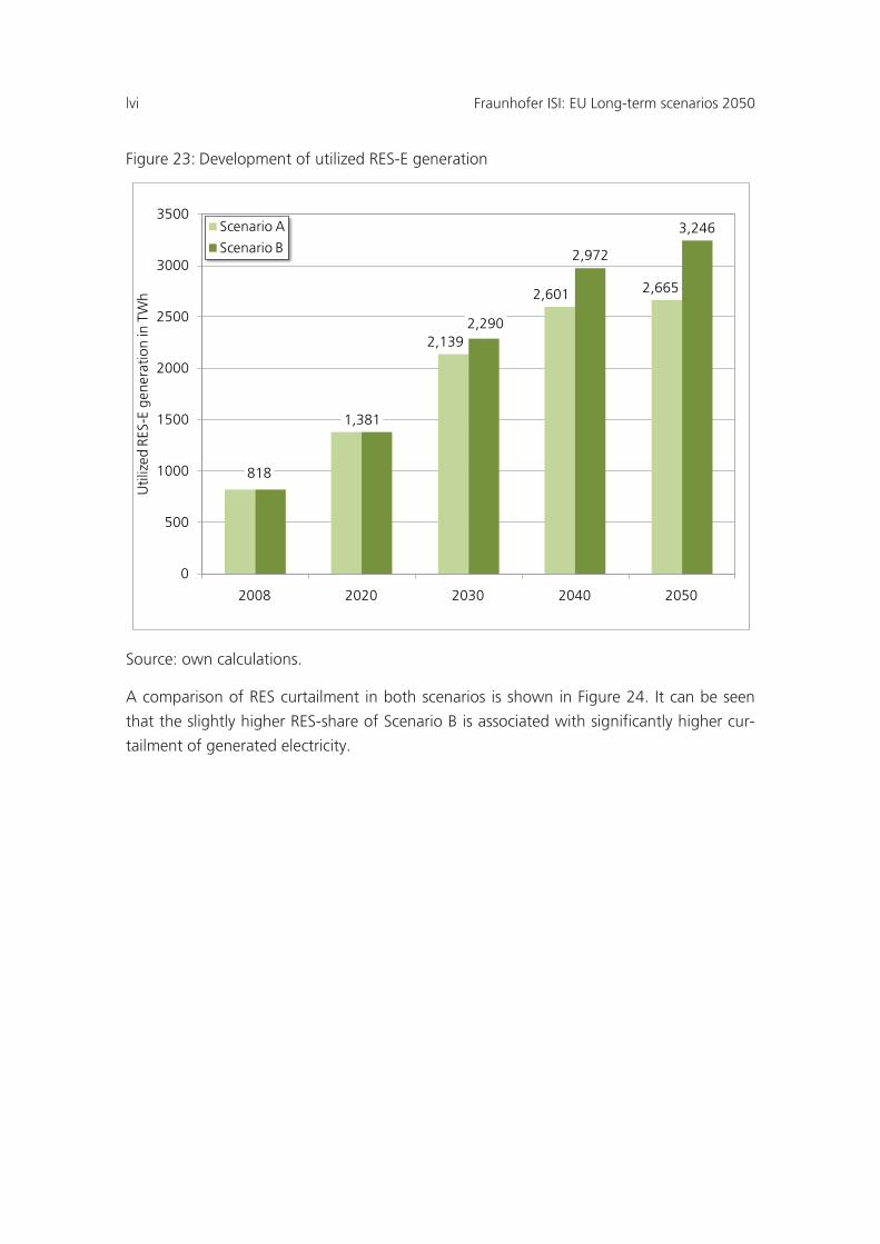
lvi Fraunhofer ISI: EU Long-term scenarios 2050
Figure 23: Development of utilized RES-E generation
Source: own calculations.
A comparison of RES curtailment in both scenarios is shown in Figure 24. It can be seen
that the slightly higher RES-share of Scenario B is associated with significantly higher cur-
tailment of generated electricity.
818
1,381
2,139
2,601 2,665
2,290
2,972
3,246
0
500
1000
1500
2000
2500
3000
3500
2008 2020 2030 2040 2050
Util
ized
RES
-E g
ener
atio
n in
TW
h
Scenario A
Scenario B
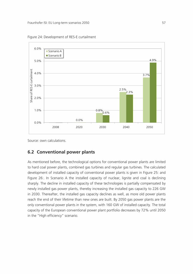
Fraunhofer ISI: EU Long-term scenarios 2050 57
Figure 24: Development of RES-E curtailment
Source: own calculations.
6.2 Conventional power plants
As mentioned before, the technological options for conventional power plants are limited
to hard coal power plants, combined gas turbines and regular gas turbines. The calculated
development of installed capacity of conventional power plants is given in Figure 25: and
Figure 26:. In Scenario A the installed capacity of nuclear, lignite and coal is declining
sharply. The decline in installed capacity of these technologies is partially compensated by
newly installed gas power plants, thereby increasing the installed gas capacity to 226 GW
in 2030. Thereafter, the installed gas capacity declines as well, as more old power plants
reach the end of their lifetime than new ones are built. By 2050 gas power plants are the
only conventional power plants in the system, with 160 GW of installed capacity. The total
capacity of the European conventional power plant portfolio decreases by 72% until 2050
in the “High efficiency” scenario.
0.8%
2.5%
3.7%
0.0%
0.6%
2.3%
4.9%
0.0%
1.0%
2.0%
3.0%
4.0%
5.0%
6.0%
2008 2020 2030 2040 2050
Shar
e of
RES
-E c
urta
ilmen
t
Scenario A
Scenario B
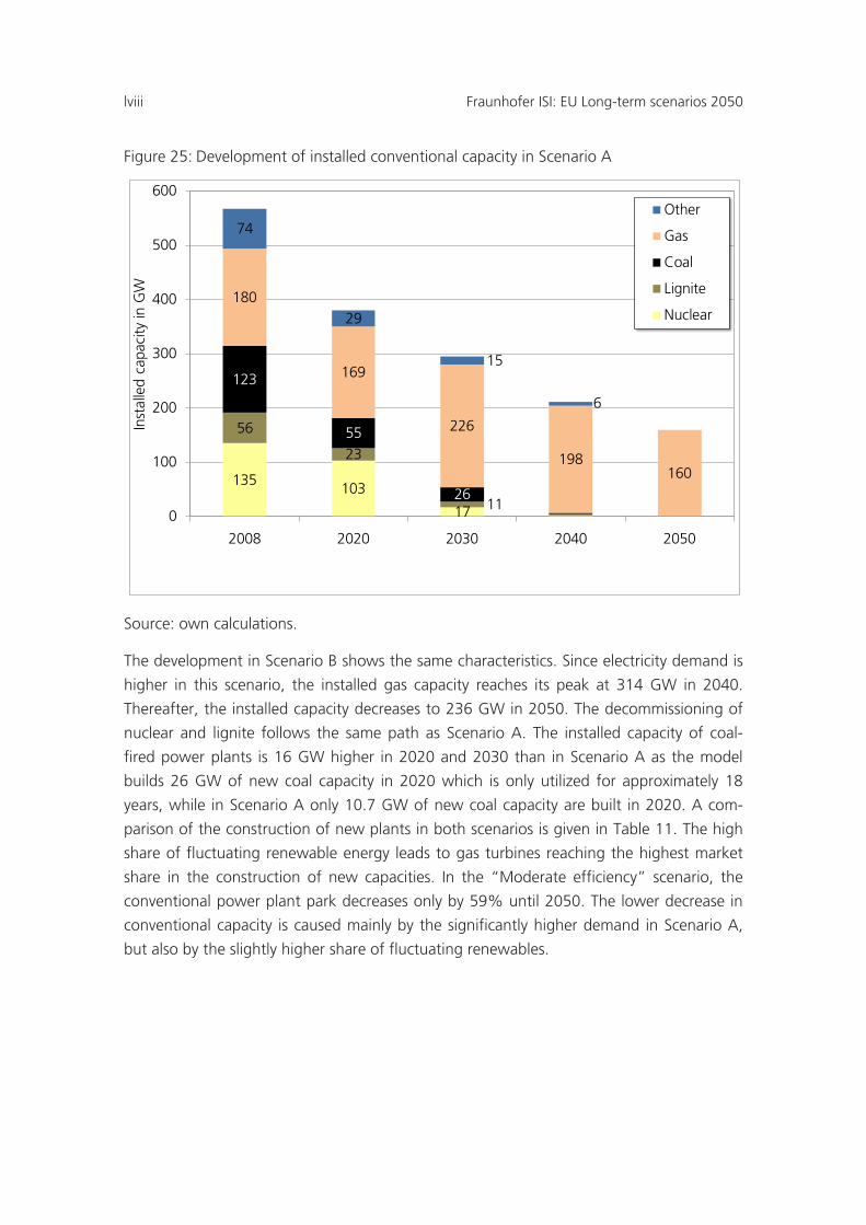
lviii Fraunhofer ISI: EU Long-term scenarios 2050
Figure 25: Development of installed conventional capacity in Scenario A
Source: own calculations.
The development in Scenario B shows the same characteristics. Since electricity demand is
higher in this scenario, the installed gas capacity reaches its peak at 314 GW in 2040.
Thereafter, the installed capacity decreases to 236 GW in 2050. The decommissioning of
nuclear and lignite follows the same path as Scenario A. The installed capacity of coal-
fired power plants is 16 GW higher in 2020 and 2030 than in Scenario A as the model
builds 26 GW of new coal capacity in 2020 which is only utilized for approximately 18
years, while in Scenario A only 10.7 GW of new coal capacity are built in 2020. A com-
parison of the construction of new plants in both scenarios is given in Table 11. The high
share of fluctuating renewable energy leads to gas turbines reaching the highest market
share in the construction of new capacities. In the “Moderate efficiency” scenario, the
conventional power plant park decreases only by 59% until 2050. The lower decrease in
conventional capacity is caused mainly by the significantly higher demand in Scenario A,
but also by the slightly higher share of fluctuating renewables.
135 103
17
56
23
11
123
55
26
180
169
226
198160
74
29
15
6
0
100
200
300
400
500
600
2008 2020 2030 2040 2050
Inst
alle
d ca
paci
ty in
GW
Other
Gas
Coal
Lignite
Nuclear
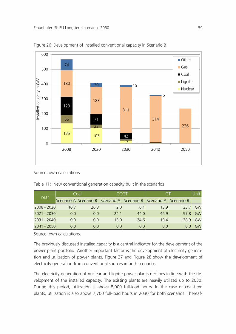
Fraunhofer ISI: EU Long-term scenarios 2050 59
Figure 26: Development of installed conventional capacity in Scenario B
Source: own calculations.
Table 11: New conventional generation capacity built in the scenarios
Year Coal CCGT GT Unit
Scenario A Scenario B Scenario A Scenario B Scenario A Scenario B
2008 - 2020 10.7 26.3 2.0 6.1 13.9 23.7 GW
2021 - 2030 0.0 0.0 24.1 44.0 46.9 97.8 GW
2031 - 2040 0.0 0.0 13.0 24.6 19.4 38.9 GW
2041 - 2050 0.0 0.0 0.0 0.0 0.0 0.0 GW
Source: own calculations.
The previously discussed installed capacity is a central indicator for the development of the
power plant portfolio. Another important factor is the development of electricity genera-
tion and utilization of power plants. Figure 27 and Figure 28 show the development of
electricity generation from conventional sources in both scenarios.
The electricity generation of nuclear and lignite power plants declines in line with the de-
velopment of the installed capacity. The existing plants are heavily utilized up to 2030.
During this period, utilization is above 8,000 full-load hours. In the case of coal-fired
plants, utilization is also above 7,700 full-load hours in 2030 for both scenarios. Thereaf-
135 103
17
56
23
11
123
71
42
180
183
311
314
236
74
29 15
6
0
100
200
300
400
500
600
2008 2020 2030 2040 2050
Inst
alle
d ca
paci
ty in
GW
Other
Gas
Coal
Lignite
Nuclear
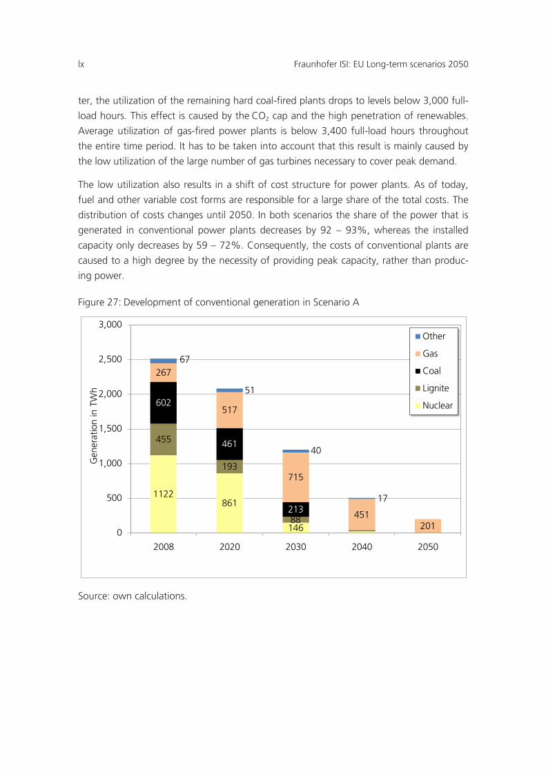
lx Fraunhofer ISI: EU Long-term scenarios 2050
ter, the utilization of the remaining hard coal-fired plants drops to levels below 3,000 full-
load hours. This effect is caused by the CO2 cap and the high penetration of renewables.
Average utilization of gas-fired power plants is below 3,400 full-load hours throughout
the entire time period. It has to be taken into account that this result is mainly caused by
the low utilization of the large number of gas turbines necessary to cover peak demand.
The low utilization also results in a shift of cost structure for power plants. As of today,
fuel and other variable cost forms are responsible for a large share of the total costs. The
distribution of costs changes until 2050. In both scenarios the share of the power that is
generated in conventional power plants decreases by 92 – 93%, whereas the installed
capacity only decreases by 59 – 72%. Consequently, the costs of conventional plants are
caused to a high degree by the necessity of providing peak capacity, rather than produc-
ing power.
Figure 27: Development of conventional generation in Scenario A
Source: own calculations.
1122861
146
455
193
88
602
461
213
267
517
715
451201
67
51
40
17
0
500
1,000
1,500
2,000
2,500
3,000
2008 2020 2030 2040 2050
Gen
erat
ion
in T
Wh
Other
Gas
Coal
Lignite
Nuclear
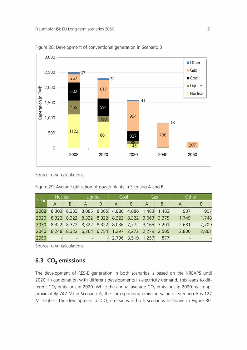
Fraunhofer ISI: EU Long-term scenarios 2050 61
Figure 28: Development of conventional generation in Scenario B
Source: own calculations.
Figure 29: Average utilization of power plants in Scenario A and B
Year Nuclear Lignite Coal Gas Other
A B A B A B A B A B
2008 8,303 8,303 8,085 8,085 4,886 4,886 1,483 1,483 907 907
2020 8,322 8,322 8,322 8,322 8,322 8,322 3,063 3,375 1,749 1,748
2030 8,322 8,322 8,322 8,322 8,036 7,772 3,165 3,201 2,681 2,709
2040 8,248 8,322 6,264 6,754 1,297 2,272 2,279 2,505 2,800 2,861
2050 - - - - 2,736 3,519 1,257 877 - -
Source: own calculations.
6.3 CO2 emissions
The development of RES-E generation in both scenarios is based on the NREAPS until
2020. In combination with different developments in electricity demand, this leads to dif-
ferent CO2 emissions in 2020. While the annual average CO2 emissions in 2020 reach ap-
proximately 742 Mt in Scenario A, the corresponding emission value of Scenario A is 127
Mt higher. The development of CO2 emissions in both scenarios is shown in Figure 30.
1122861
146
455
193
88
602
591
327
267
617
994
786
207
6751
41
18
0
500
1,000
1,500
2,000
2,500
3,000
2008 2020 2030 2040 2050
Gen
erat
ion
in T
Wh
Other
Gas
Coal
Lignite
Nuclear
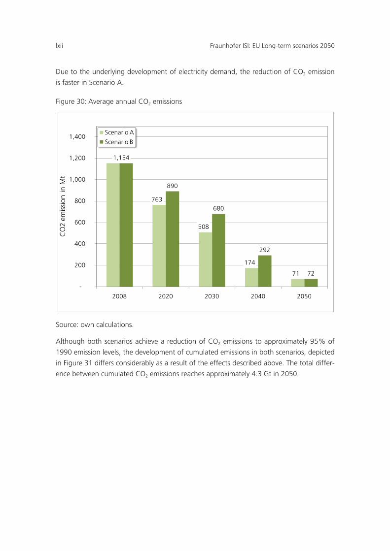
lxii Fraunhofer ISI: EU Long-term scenarios 2050
Due to the underlying development of electricity demand, the reduction of CO2 emission
is faster in Scenario A.
Figure 30: Average annual CO2 emissions
Source: own calculations.
Although both scenarios achieve a reduction of CO2 emissions to approximately 95% of
1990 emission levels, the development of cumulated emissions in both scenarios, depicted
in Figure 31 differs considerably as a result of the effects described above. The total differ-
ence between cumulated CO2 emissions reaches approximately 4.3 Gt in 2050.
1,154
763
508
174
71
890
680
292
72
-
200
400
600
800
1,000
1,200
1,400
2008 2020 2030 2040 2050
CO
2 em
issi
on i
n M
t
Scenario A
Scenario B
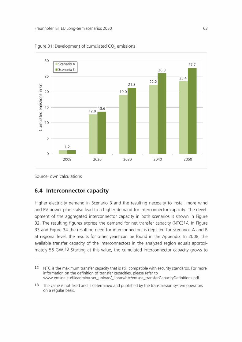
Fraunhofer ISI: EU Long-term scenarios 2050 63
Figure 31: Development of cumulated CO2 emissions
Source: own calculations
6.4 Interconnector capacity
Higher electricity demand in Scenario B and the resulting necessity to install more wind
and PV power plants also lead to a higher demand for interconnector capacity. The devel-
opment of the aggregated interconnector capacity in both scenarios is shown in Figure
32. The resulting figures express the demand for net transfer capacity (NTC)12 Figure
33
. In
and Figure 34 the resulting need for interconnectors is depicted for scenarios A and B
at regional level, the results for other years can be found in the Appendix. In 2008, the
available transfer capacity of the interconnectors in the analyzed region equals approxi-
mately 56 GW.13
12 NTC is the maximum transfer capacity that is still compatible with security standards. For more information on the definition of transfer capacities, please refer to www.entsoe.eu/fileadmin/user_upload/_library/ntc/entsoe_transferCapacityDefinitions.pdf.
Starting at this value, the cumulated interconnector capacity grows to
13 The value is not fixed and is determined and published by the transmission system operators on a regular basis.
1.2
12.8
19.0
22.223.4
13.6
21.3
26.027.7
0
5
10
15
20
25
30
2008 2020 2030 2040 2050
Cum
ulat
ed e
mis
sion
s in
Gt
Scenario A
Scenario B
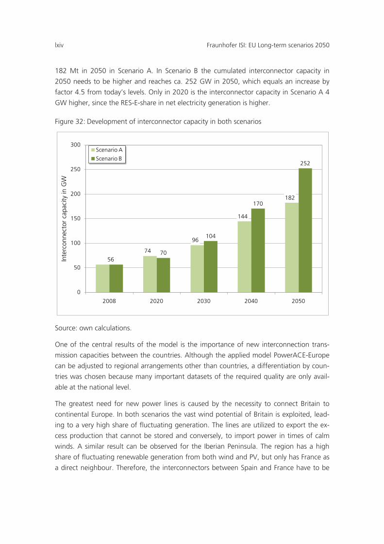
lxiv Fraunhofer ISI: EU Long-term scenarios 2050
182 Mt in 2050 in Scenario A. In Scenario B the cumulated interconnector capacity in
2050 needs to be higher and reaches ca. 252 GW in 2050, which equals an increase by
factor 4.5 from today’s levels. Only in 2020 is the interconnector capacity in Scenario A 4
GW higher, since the RES-E-share in net electricity generation is higher.
Figure 32: Development of interconnector capacity in both scenarios
Source: own calculations.
One of the central results of the model is the importance of new interconnection trans-
mission capacities between the countries. Although the applied model PowerACE-Europe
can be adjusted to regional arrangements other than countries, a differentiation by coun-
tries was chosen because many important datasets of the required quality are only avail-
able at the national level.
The greatest need for new power lines is caused by the necessity to connect Britain to
continental Europe. In both scenarios the vast wind potential of Britain is exploited, lead-
ing to a very high share of fluctuating generation. The lines are utilized to export the ex-
cess production that cannot be stored and conversely, to import power in times of calm
winds. A similar result can be observed for the Iberian Peninsula. The region has a high
share of fluctuating renewable generation from both wind and PV, but only has France as
a direct neighbour. Therefore, the interconnectors between Spain and France have to be
56
74
96
144
182
70
104
170
252
0
50
100
150
200
250
300
2008 2020 2030 2040 2050
Inte
rcon
nect
or c
apac
ity in
GW
Scenario A
Scenario B
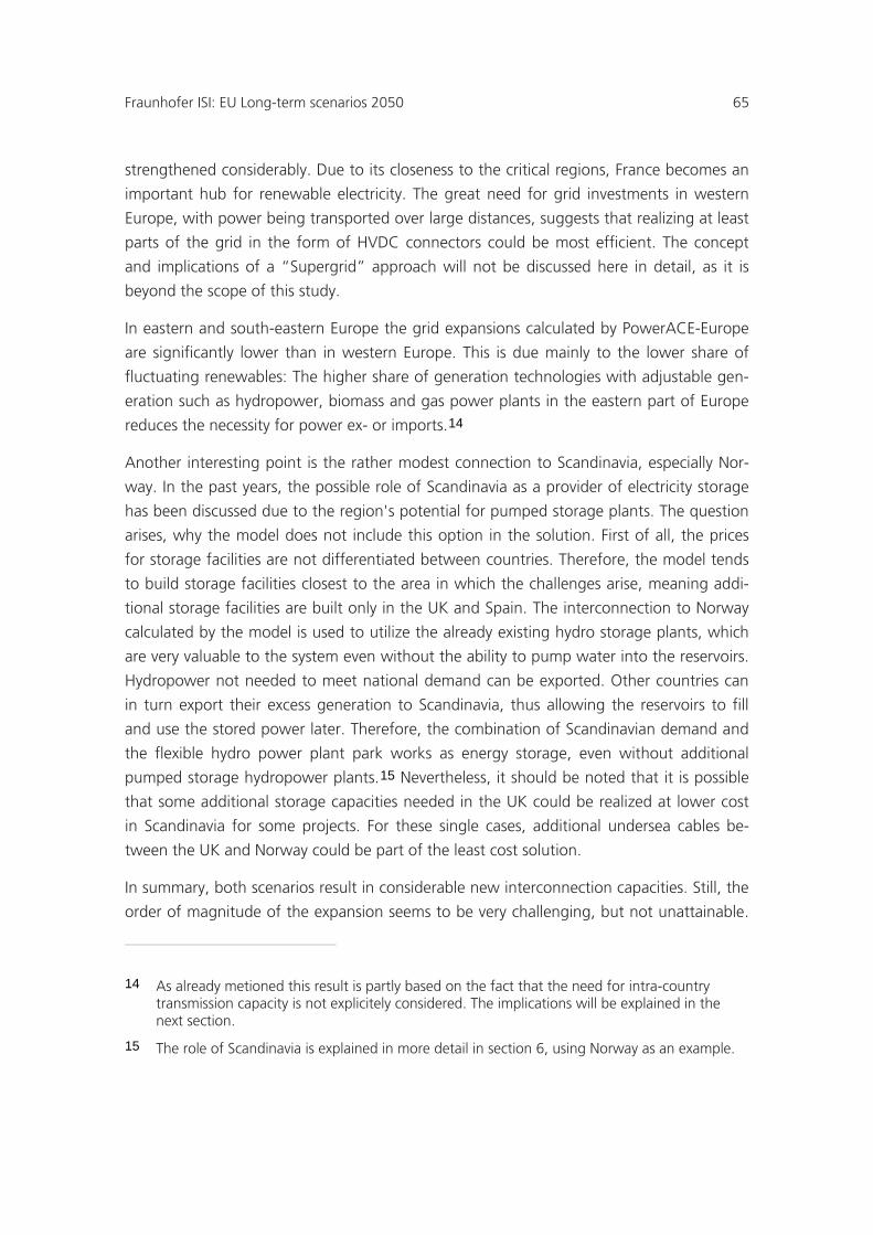
Fraunhofer ISI: EU Long-term scenarios 2050 65
strengthened considerably. Due to its closeness to the critical regions, France becomes an
important hub for renewable electricity. The great need for grid investments in western
Europe, with power being transported over large distances, suggests that realizing at least
parts of the grid in the form of HVDC connectors could be most efficient. The concept
and implications of a “Supergrid” approach will not be discussed here in detail, as it is
beyond the scope of this study.
In eastern and south-eastern Europe the grid expansions calculated by PowerACE-Europe
are significantly lower than in western Europe. This is due mainly to the lower share of
fluctuating renewables: The higher share of generation technologies with adjustable gen-
eration such as hydropower, biomass and gas power plants in the eastern part of Europe
reduces the necessity for power ex- or imports.14
Another interesting point is the rather modest connection to Scandinavia, especially Nor-
way. In the past years, the possible role of Scandinavia as a provider of electricity storage
has been discussed due to the region's potential for pumped storage plants. The question
arises, why the model does not include this option in the solution. First of all, the prices
for storage facilities are not differentiated between countries. Therefore, the model tends
to build storage facilities closest to the area in which the challenges arise, meaning addi-
tional storage facilities are built only in the UK and Spain. The interconnection to Norway
calculated by the model is used to utilize the already existing hydro storage plants, which
are very valuable to the system even without the ability to pump water into the reservoirs.
Hydropower not needed to meet national demand can be exported. Other countries can
in turn export their excess generation to Scandinavia, thus allowing the reservoirs to fill
and use the stored power later. Therefore, the combination of Scandinavian demand and
the flexible hydro power plant park works as energy storage, even without additional
pumped storage hydropower plants.
15
In summary, both scenarios result in considerable new interconnection capacities. Still, the
order of magnitude of the expansion seems to be very challenging, but not unattainable.
Nevertheless, it should be noted that it is possible
that some additional storage capacities needed in the UK could be realized at lower cost
in Scandinavia for some projects. For these single cases, additional undersea cables be-
tween the UK and Norway could be part of the least cost solution.
14 As already metioned this result is partly based on the fact that the need for intra-country transmission capacity is not explicitely considered. The implications will be explained in the next section.
15 The role of Scandinavia is explained in more detail in section 6, using Norway as an example.
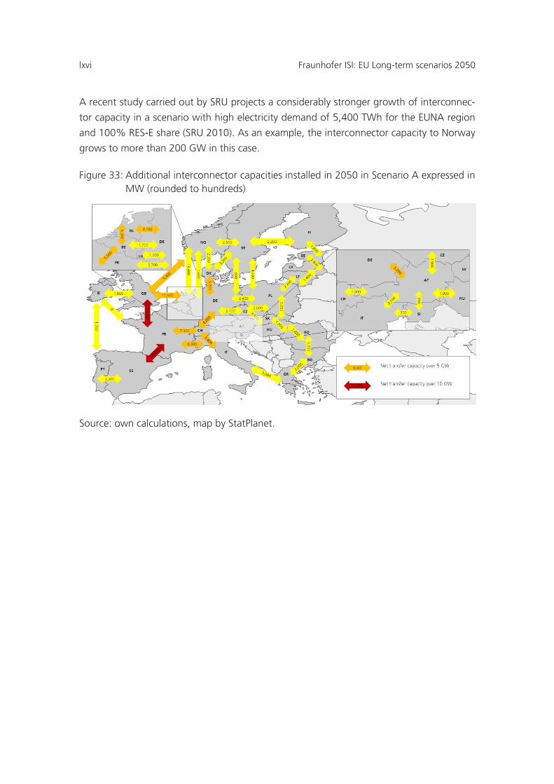
lxvi Fraunhofer ISI: EU Long-term scenarios 2050
A recent study carried out by SRU projects a considerably stronger growth of interconnec-
tor capacity in a scenario with high electricity demand of 5,400 TWh for the EUNA region
and 100% RES-E share (SRU 2010). As an example, the interconnector capacity to Norway
grows to more than 200 GW in this case.
Figure 33: Additional interconnector capacities installed in 2050 in Scenario A expressed in MW (rounded to hundreds)
Source: own calculations, map by StatPlanet.
Fraunhofer ISI: EU Long-term scenarios 2050 67
Figure 34: Additional interconnector capacities installed in 2050 in Scenario B expressed in MW (rounded to hundreds)
Source: own calculations, map by StatPlanet.
6.4.1 Implications for national transport grids and electricity distri-bution grids
The results presented above only cover the net transfer capacity between countries, i.e.
the power lines and cables used to exchange power between countries, while other com-
ponents of the grid are not included. This simplification implies that the countries do not
have transmission bottlenecks within their borders. This means that the transport and dis-
tribution grids do not restrict the flow of electricity at any time. Electricity generated at
any location in the respective country can either be consumed at any location in the coun-
try or be exported to any country. The occurring losses are taken into account in the
model, either implicitly for losses within the country of origin, or explicitly for exports. In
the model, situations in which the transport or distribution within countries are congested
are not taken into account.
Consequently, the modelling approach used in this study covers a significant share of the
European grid, but assumes that the remaining parts are developed adequately. If this is
not the case, for some hours more RES-E generation would have to be curtailed than es-
timated by the model. This restriction is not as challenging as it might seem, for two rea-
sons. First of all, the interconnection lines presented above are calculated between
weighted centres of demand. This means that they act as strong backbones connecting
major demand centres that are also available for transport within the countries. Secondly,
lxviii Fraunhofer ISI: EU Long-term scenarios 2050
the transport lines within the countries are mostly congested during very windy hours. At
these times, curtailment is already taking place in the model anyway, since the intercon-
necting lines are not designed to transport all the power produced at any time. This
means that although congestion might occur on the transport lines within the countries,
this is most likely superposed by the curtailment induced by the congested interconnectors
in windy hours.
Modelling the remaining transport grid individually requires explicit modelling of each
power line and a very detailed knowledge about the location of both load centres and
generation capacities. Although this is possible, the immensely increased calculating time
would require simplifications in other aspects of the model. Modelling the lower voltage
levels of the distribution grid is even more challenging and not possible for a model cover-
ing Europe as a whole. It is clear that the changes in the structure of electricity generation
towards decentralized generation require new grid concepts. Especially the high growth
rates of PV will become a challenge in this context. Nevertheless, a detailed modelling of
the remaining transport and distribution grid is beyond the scope and possibilities of this
study. Improving this aspect will be a task for future studies.
6.5 Storage capacity
Another important result of the scenario calculations is the development of storage capac-
ity. The development of cumulated storage capacities is given in Figure 35. The figure
shows two steps in the development of storage capacities. The first step takes place be-
tween 2008 and 2020. The available storage capacity increases by ca. 7 GW. This increase
is based on projects that are already planned or are under construction. Thereafter storage
capacity remains constant in both scenarios. The next step takes place in 2050 when the
effective RES-E share increases to more than 90%. In Scenario A, 3.3 GW additional stor-
age capacity is built. In Scenario B approximately 5 GW of additional storage capacity is
built. The very low demand for additional storage capacity is a remarkable result.
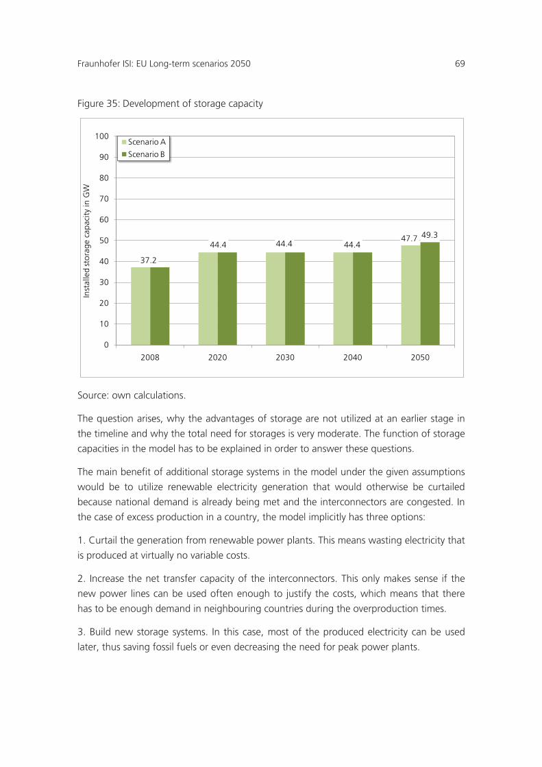
Fraunhofer ISI: EU Long-term scenarios 2050 69
Figure 35: Development of storage capacity
Source: own calculations.
The question arises, why the advantages of storage are not utilized at an earlier stage in
the timeline and why the total need for storages is very moderate. The function of storage
capacities in the model has to be explained in order to answer these questions.
The main benefit of additional storage systems in the model under the given assumptions
would be to utilize renewable electricity generation that would otherwise be curtailed
because national demand is already being met and the interconnectors are congested. In
the case of excess production in a country, the model implicitly has three options:
1. Curtail the generation from renewable power plants. This means wasting electricity that
is produced at virtually no variable costs.
2. Increase the net transfer capacity of the interconnectors. This only makes sense if the
new power lines can be used often enough to justify the costs, which means that there
has to be enough demand in neighbouring countries during the overproduction times.
3. Build new storage systems. In this case, most of the produced electricity can be used
later, thus saving fossil fuels or even decreasing the need for peak power plants.
37.2
44.4 44.4 44.447.7 49.3
0
10
20
30
40
50
60
70
80
90
100
2008 2020 2030 2040 2050
Inst
alle
d st
orag
e ca
paci
ty in
GW
Scenario A
Scenario B
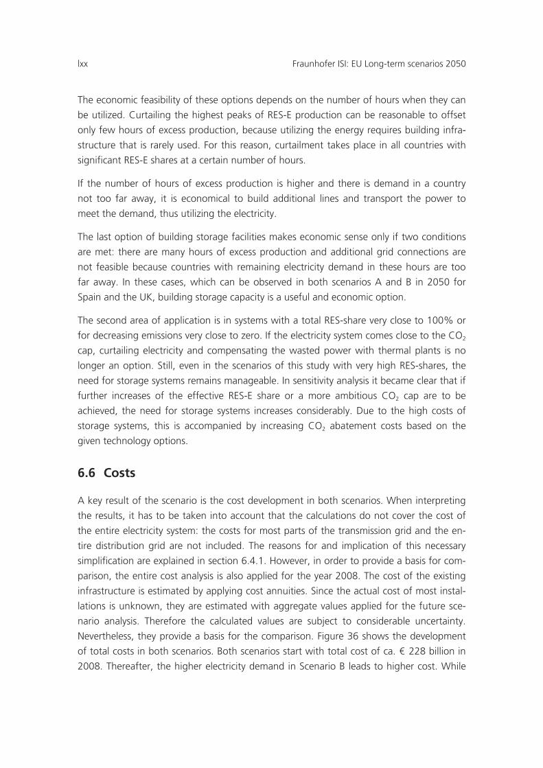
lxx Fraunhofer ISI: EU Long-term scenarios 2050
The economic feasibility of these options depends on the number of hours when they can
be utilized. Curtailing the highest peaks of RES-E production can be reasonable to offset
only few hours of excess production, because utilizing the energy requires building infra-
structure that is rarely used. For this reason, curtailment takes place in all countries with
significant RES-E shares at a certain number of hours.
If the number of hours of excess production is higher and there is demand in a country
not too far away, it is economical to build additional lines and transport the power to
meet the demand, thus utilizing the electricity.
The last option of building storage facilities makes economic sense only if two conditions
are met: there are many hours of excess production and additional grid connections are
not feasible because countries with remaining electricity demand in these hours are too
far away. In these cases, which can be observed in both scenarios A and B in 2050 for
Spain and the UK, building storage capacity is a useful and economic option.
The second area of application is in systems with a total RES-share very close to 100% or
for decreasing emissions very close to zero. If the electricity system comes close to the CO2
cap, curtailing electricity and compensating the wasted power with thermal plants is no
longer an option. Still, even in the scenarios of this study with very high RES-shares, the
need for storage systems remains manageable. In sensitivity analysis it became clear that if
further increases of the effective RES-E share or a more ambitious CO2 cap are to be
achieved, the need for storage systems increases considerably. Due to the high costs of
storage systems, this is accompanied by increasing CO2 abatement costs based on the
given technology options.
6.6 Costs
A key result of the scenario is the cost development in both scenarios. When interpreting
the results, it has to be taken into account that the calculations do not cover the cost of
the entire electricity system: the costs for most parts of the transmission grid and the en-
tire distribution grid are not included. The reasons for and implication of this necessary
simplification are explained in section 6.4.1. However, in order to provide a basis for com-
parison, the entire cost analysis is also applied for the year 2008. The cost of the existing
infrastructure is estimated by applying cost annuities. Since the actual cost of most instal-
lations is unknown, they are estimated with aggregate values applied for the future sce-
nario analysis. Therefore the calculated values are subject to considerable uncertainty.
Nevertheless, they provide a basis for the comparison. Figure 36 shows the development
of total costs in both scenarios. Both scenarios start with total cost of ca. € 228 billion in
2008. Thereafter, the higher electricity demand in Scenario B leads to higher cost. While
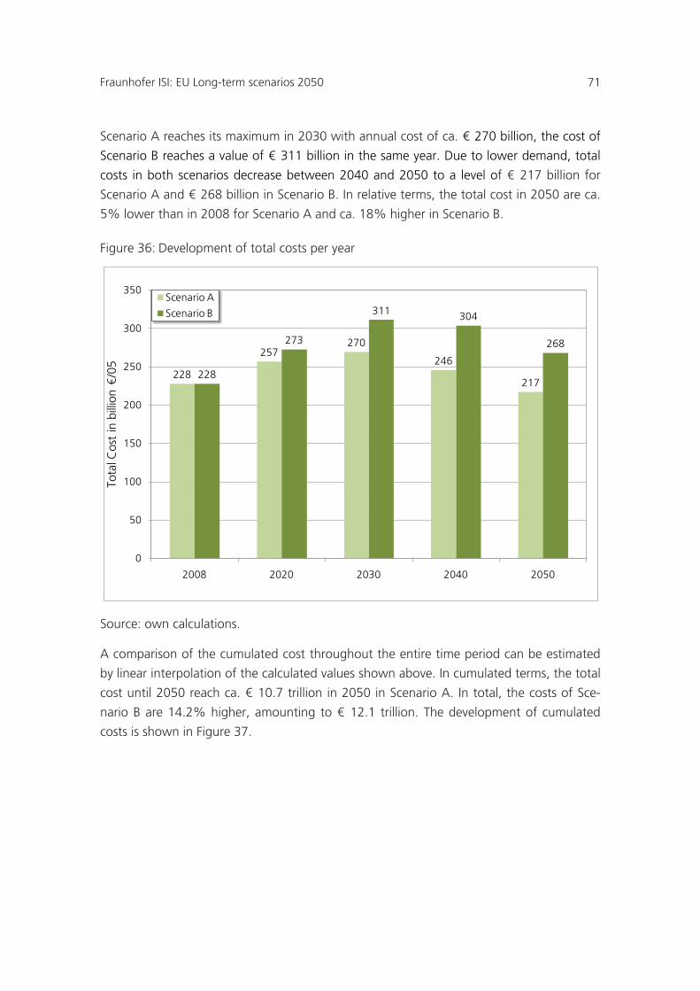
Fraunhofer ISI: EU Long-term scenarios 2050 71
Scenario A reaches its maximum in 2030 with annual cost of ca. € 270 billion, the cost of
Scenario B reaches a value of € 311 billion in the same year. Due to lower demand, total
costs in both scenarios decrease between 2040 and 2050 to a level of € 217 billion for
Scenario A and € 268 billion in Scenario B. In relative terms, the total cost in 2050 are ca.
5% lower than in 2008 for Scenario A and ca. 18% higher in Scenario B.
Figure 36: Development of total costs per year
Source: own calculations.
A comparison of the cumulated cost throughout the entire time period can be estimated
by linear interpolation of the calculated values shown above. In cumulated terms, the total
cost until 2050 reach ca. € 10.7 trillion in 2050 in Scenario A. In total, the costs of Sce-
nario B are 14.2% higher, amounting to € 12.1 trillion. The development of cumulated
costs is shown in Figure 37.
228
257270
246
217228
273
311 304
268
0
50
100
150
200
250
300
350
2008 2020 2030 2040 2050
Tota
l Cos
t in
bill
ion
€/0
5
Scenario A
Scenario B
lxxii Fraunhofer ISI: EU Long-term scenarios 2050
Figure 37: Development of cumulated costs
Source: own calculations.
Another important perspective in analysing the development of the cost of the electricity
system is the development of specific cost per MWh. The development of specific cost is
given in Figure 38. Both scenarios start with specific costs of 74.5 €/MWh. In both scenar-
ios specific costs increase over the next decades. While Scenario A reaches its peak in spe-
cific costs with ca. 88.0 €/MWh in 2030, the total cost of Scenario A reaches a slightly
lower value of 87.3 €/MWh. The comparison of both scenarios shows that specific costs in
both scenarios reach a similar level in the period 2020-2040. However, in 2050 the spe-
cific cost of Scenario A is 2.1 €/MWh or ca. 2.4 % lower. Despite the ambitious reduction
of CO2 emissions, the specific costs in 2050 are only 13% (Scenario A) and 15.4% (Sce-
nario B) higher than in 2008. As the analysis does not include most parts of the grid costs,
the increase of the entire cost of electricity supply is likely to be higher, since the increase
in RES-E generation and interconnector capacity is also likely to require strengthening na-
tional grid infrastructures.
0.2
3.2
5.8
8.4
10.7
0.2
3.3
6.2
9.3
12.1
0
2
4
6
8
10
12
14
2008 2020 2030 2040 2050
Cum
ulat
ed c
ost
in t
rillio
n €
05
Scenario A
Scenario B
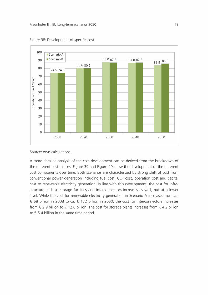
Fraunhofer ISI: EU Long-term scenarios 2050 73
Figure 38: Development of specific cost
Source: own calculations.
A more detailed analysis of the cost development can be derived from the breakdown of
the different cost factors. Figure 39 and Figure 40 show the development of the different
cost components over time. Both scenarios are characterized by strong shift of cost from
conventional power generation including fuel cost, CO2 cost, operation cost and capital
cost to renewable electricity generation. In line with this development, the cost for infra-
structure such as storage facilities and interconnectors increases as well, but at a lower
level. While the cost for renewable electricity generation in Scenario A increases from ca.
€ 58 billion in 2008 to ca. € 172 billion in 2050, the cost for interconnectors increases
from € 2.9 billion to € 12.6 billion. The cost for storage plants increases from € 4.2 billion
to € 5.4 billion in the same time period.
74.5
80.6
88.0 87.083.9
74.580.2
87.3 87.3 86.0
0
10
20
30
40
50
60
70
80
90
100
2008 2020 2030 2040 2050
Spec
ific
cost
in €
/MW
h
Scenario A
Scenario B
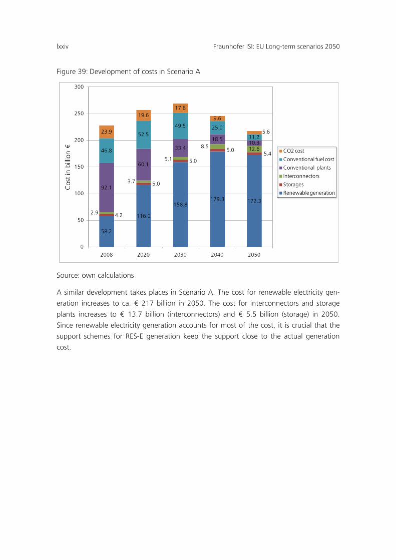
lxxiv Fraunhofer ISI: EU Long-term scenarios 2050
Figure 39: Development of costs in Scenario A
Source: own calculations
A similar development takes places in Scenario A. The cost for renewable electricity gen-
eration increases to ca. € 217 billion in 2050. The cost for interconnectors and storage
plants increases to € 13.7 billion (interconnectors) and € 5.5 billion (storage) in 2050.
Since renewable electricity generation accounts for most of the cost, it is crucial that the
support schemes for RES-E generation keep the support close to the actual generation
cost.
58.2
116.0
158.8179.3 172.3
4.2
5.0
5.0
5.05.4
2.9
3.7
5.1
8.5 12.6
92.1
60.1
33.4
18.510.3
46.8
52.5
49.5 25.0
11.223.9
19.617.8
9.6
5.6
0
50
100
150
200
250
300
2008 2020 2030 2040 2050
Cos
t in
bill
ion
€
CO2 cost
Conventional fuel cost
Conventional plants
Interconnectors
Storages
Renewable generation
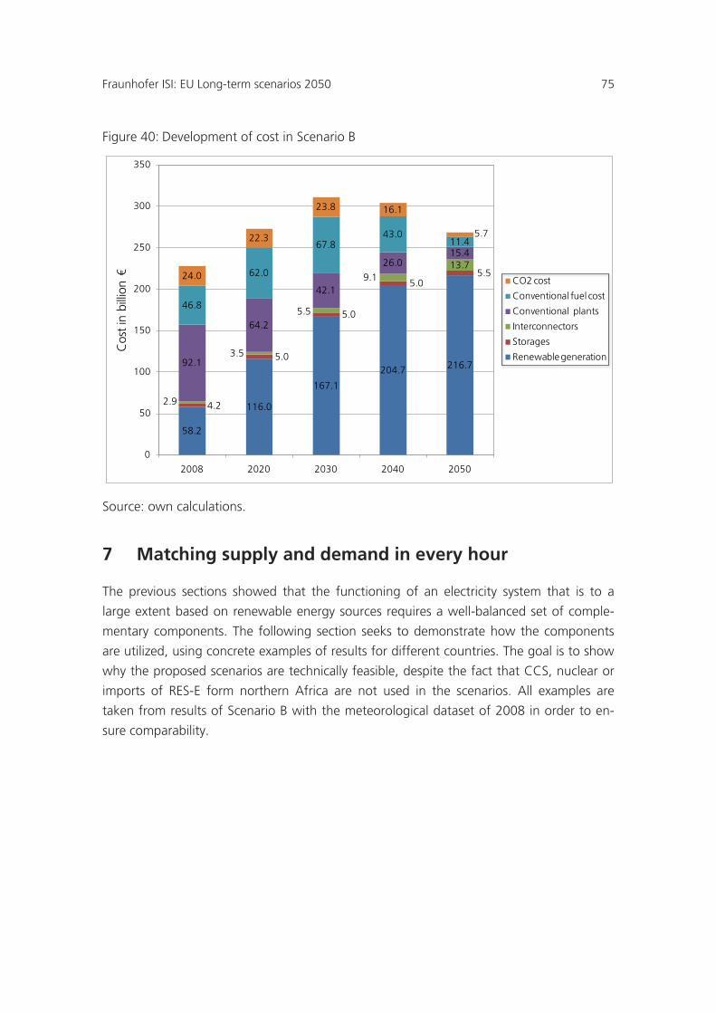
Fraunhofer ISI: EU Long-term scenarios 2050 75
Figure 40: Development of cost in Scenario B
Source: own calculations.
7 Matching supply and demand in every hour
The previous sections showed that the functioning of an electricity system that is to a
large extent based on renewable energy sources requires a well-balanced set of comple-
mentary components. The following section seeks to demonstrate how the components
are utilized, using concrete examples of results for different countries. The goal is to show
why the proposed scenarios are technically feasible, despite the fact that CCS, nuclear or
imports of RES-E form northern Africa are not used in the scenarios. All examples are
taken from results of Scenario B with the meteorological dataset of 2008 in order to en-
sure comparability.
58.2
116.0
167.1
204.7 216.7
4.2
5.0
5.0
5.05.5
2.9
3.5
5.5
9.113.7
92.1
64.2
42.1
26.015.4
46.8
62.0
67.843.0
11.4
24.0
22.3
23.8 16.1
5.7
0
50
100
150
200
250
300
350
2008 2020 2030 2040 2050
Cos
t in
bill
ion
€
CO2 cost
Conventional fuel cost
Conventional plants
Interconnectors
Storages
Renewable generation
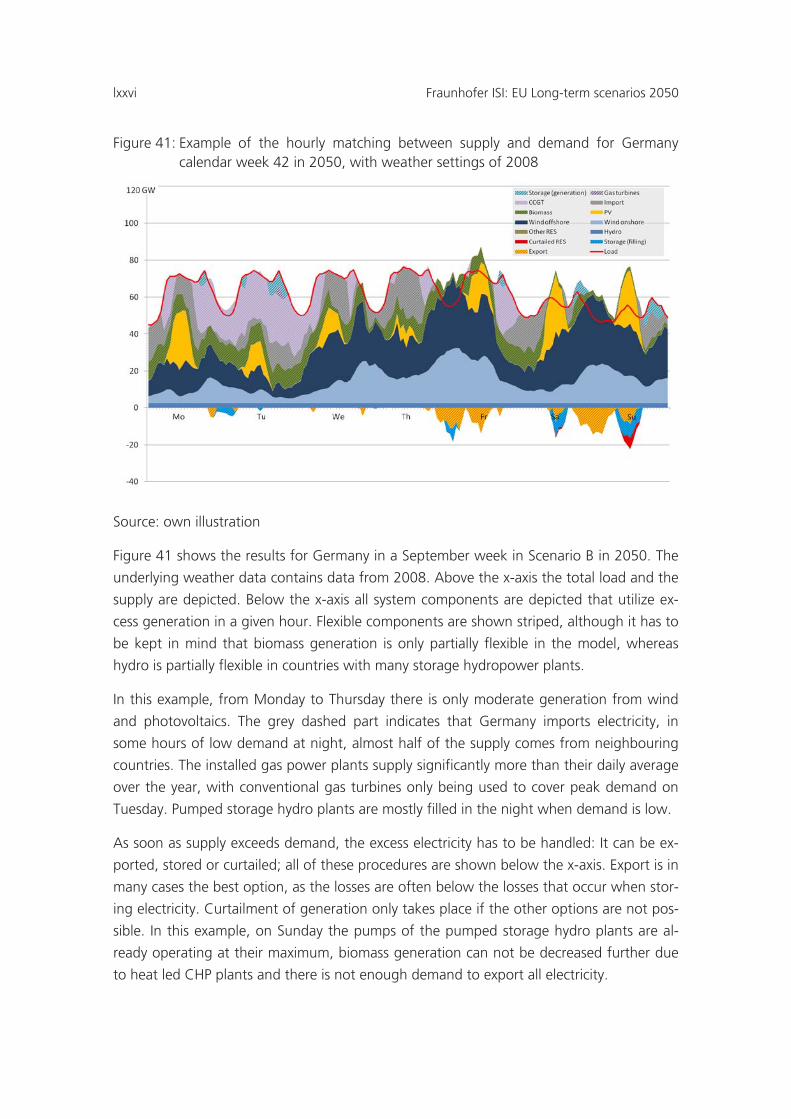
lxxvi Fraunhofer ISI: EU Long-term scenarios 2050
Figure 41: Example of the hourly matching between supply and demand for Germany calendar week 42 in 2050, with weather settings of 2008
Source: own illustration
Figure 41 shows the results for Germany in a September week in Scenario B in 2050. The
underlying weather data contains data from 2008. Above the x-axis the total load and the
supply are depicted. Below the x-axis all system components are depicted that utilize ex-
cess generation in a given hour. Flexible components are shown striped, although it has to
be kept in mind that biomass generation is only partially flexible in the model, whereas
hydro is partially flexible in countries with many storage hydropower plants.
In this example, from Monday to Thursday there is only moderate generation from wind
and photovoltaics. The grey dashed part indicates that Germany imports electricity, in
some hours of low demand at night, almost half of the supply comes from neighbouring
countries. The installed gas power plants supply significantly more than their daily average
over the year, with conventional gas turbines only being used to cover peak demand on
Tuesday. Pumped storage hydro plants are mostly filled in the night when demand is low.
As soon as supply exceeds demand, the excess electricity has to be handled: It can be ex-
ported, stored or curtailed; all of these procedures are shown below the x-axis. Export is in
many cases the best option, as the losses are often below the losses that occur when stor-
ing electricity. Curtailment of generation only takes place if the other options are not pos-
sible. In this example, on Sunday the pumps of the pumped storage hydro plants are al-
ready operating at their maximum, biomass generation can not be decreased further due
to heat led CHP plants and there is not enough demand to export all electricity.
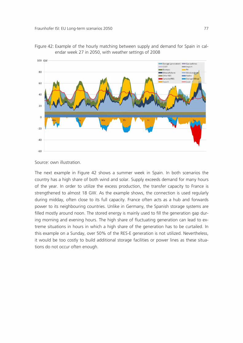
Fraunhofer ISI: EU Long-term scenarios 2050 77
Figure 42: Example of the hourly matching between supply and demand for Spain in cal-endar week 27 in 2050, with weather settings of 2008
Source: own illustration.
The next example in Figure 42 shows a summer week in Spain. In both scenarios the
country has a high share of both wind and solar. Supply exceeds demand for many hours
of the year. In order to utilize the excess production, the transfer capacity to France is
strengthened to almost 18 GW. As the example shows, the connection is used regularly
during midday, often close to its full capacity. France often acts as a hub and forwards
power to its neighbouring countries. Unlike in Germany, the Spanish storage systems are
filled mostly around noon. The stored energy is mainly used to fill the generation gap dur-
ing morning and evening hours. The high share of fluctuating generation can lead to ex-
treme situations in hours in which a high share of the generation has to be curtailed. In
this example on a Sunday, over 50% of the RES-E generation is not utilized. Nevertheless,
it would be too costly to build additional storage facilities or power lines as these situa-
tions do not occur often enough.
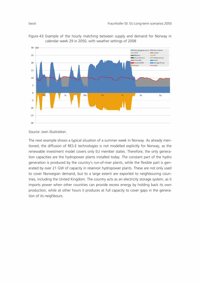
lxxviii Fraunhofer ISI: EU Long-term scenarios 2050
Figure 43: Example of the hourly matching between supply and demand for Norway in calendar week 29 in 2050, with weather settings of 2008
Source: own illustration.
The next example shows a typical situation of a summer week in Norway. As already men-
tioned, the diffusion of RES-E technologies is not modelled explicitly for Norway, as the
renewable investment model covers only EU member states. Therefore, the only genera-
tion capacities are the hydropower plants installed today. The constant part of the hydro
generation is produced by the country’s run-of-river plants, while the flexible part is gen-
erated by over 21 GW of capacity in reservoir hydropower plants. These are not only used
to cover Norwegian demand, but to a large extent are exported to neighbouring coun-
tries, including the United Kingdom. The country acts as an electricity storage system, as it
imports power when other countries can provide excess energy by holding back its own
production, while at other hours it produces at full capacity to cover gaps in the genera-
tion of its neighbours.
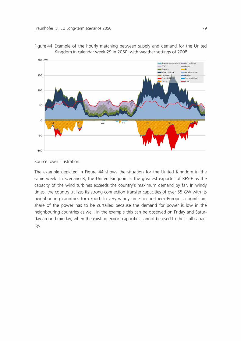
Fraunhofer ISI: EU Long-term scenarios 2050 79
Figure 44: Example of the hourly matching between supply and demand for the United Kingdom in calendar week 29 in 2050, with weather settings of 2008
Source: own illustration.
The example depicted in Figure 44 shows the situation for the United Kingdom in the
same week. In Scenario B, the United Kingdom is the greatest exporter of RES-E as the
capacity of the wind turbines exceeds the country’s maximum demand by far. In windy
times, the country utilizes its strong connection transfer capacities of over 55 GW with its
neighbouring countries for export. In very windy times in northern Europe, a significant
share of the power has to be curtailed because the demand for power is low in the
neighbouring countries as well. In the example this can be observed on Friday and Satur-
day around midday, when the existing export capacities cannot be used to their full capac-
ity.
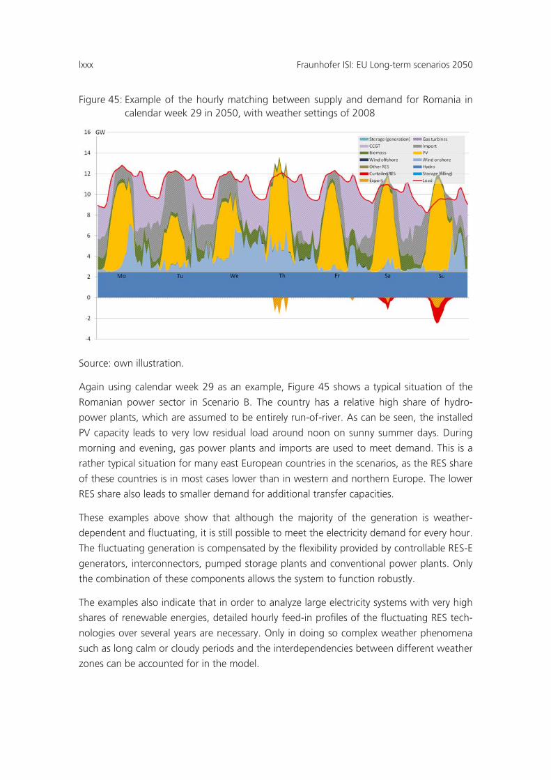
lxxx Fraunhofer ISI: EU Long-term scenarios 2050
Figure 45: Example of the hourly matching between supply and demand for Romania in calendar week 29 in 2050, with weather settings of 2008
Source: own illustration.
Again using calendar week 29 as an example, Figure 45 shows a typical situation of the
Romanian power sector in Scenario B. The country has a relative high share of hydro-
power plants, which are assumed to be entirely run-of-river. As can be seen, the installed
PV capacity leads to very low residual load around noon on sunny summer days. During
morning and evening, gas power plants and imports are used to meet demand. This is a
rather typical situation for many east European countries in the scenarios, as the RES share
of these countries is in most cases lower than in western and northern Europe. The lower
RES share also leads to smaller demand for additional transfer capacities.
These examples above show that although the majority of the generation is weather-
dependent and fluctuating, it is still possible to meet the electricity demand for every hour.
The fluctuating generation is compensated by the flexibility provided by controllable RES-E
generators, interconnectors, pumped storage plants and conventional power plants. Only
the combination of these components allows the system to function robustly.
The examples also indicate that in order to analyze large electricity systems with very high
shares of renewable energies, detailed hourly feed-in profiles of the fluctuating RES tech-
nologies over several years are necessary. Only in doing so complex weather phenomena
such as long calm or cloudy periods and the interdependencies between different weather
zones can be accounted for in the model.
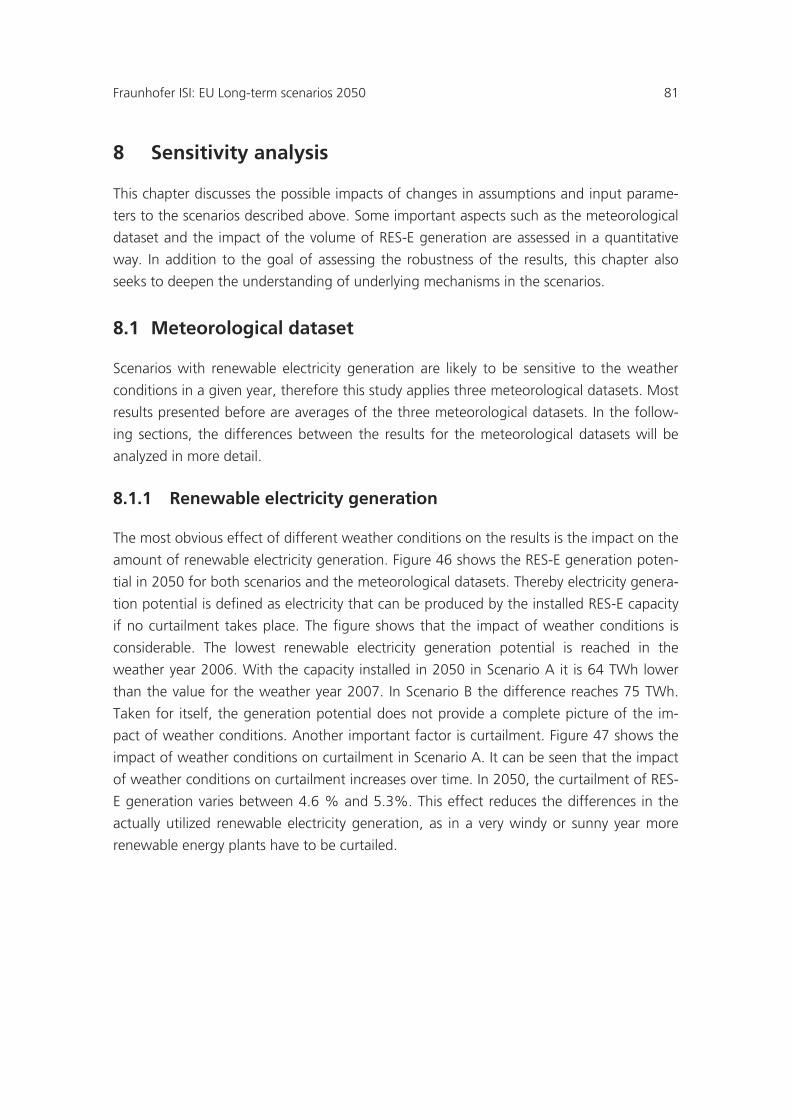
Fraunhofer ISI: EU Long-term scenarios 2050 81
8 Sensitivity analysis
This chapter discusses the possible impacts of changes in assumptions and input parame-
ters to the scenarios described above. Some important aspects such as the meteorological
dataset and the impact of the volume of RES-E generation are assessed in a quantitative
way. In addition to the goal of assessing the robustness of the results, this chapter also
seeks to deepen the understanding of underlying mechanisms in the scenarios.
8.1 Meteorological dataset
Scenarios with renewable electricity generation are likely to be sensitive to the weather
conditions in a given year, therefore this study applies three meteorological datasets. Most
results presented before are averages of the three meteorological datasets. In the follow-
ing sections, the differences between the results for the meteorological datasets will be
analyzed in more detail.
8.1.1 Renewable electricity generation
The most obvious effect of different weather conditions on the results is the impact on the
amount of renewable electricity generation. Figure 46 shows the RES-E generation poten-
tial in 2050 for both scenarios and the meteorological datasets. Thereby electricity genera-
tion potential is defined as electricity that can be produced by the installed RES-E capacity
if no curtailment takes place. The figure shows that the impact of weather conditions is
considerable. The lowest renewable electricity generation potential is reached in the
weather year 2006. With the capacity installed in 2050 in Scenario A it is 64 TWh lower
than the value for the weather year 2007. In Scenario B the difference reaches 75 TWh.
Taken for itself, the generation potential does not provide a complete picture of the im-
pact of weather conditions. Another important factor is curtailment. Figure 47 shows the
impact of weather conditions on curtailment in Scenario A. It can be seen that the impact
of weather conditions on curtailment increases over time. In 2050, the curtailment of RES-
E generation varies between 4.6 % and 5.3%. This effect reduces the differences in the
actually utilized renewable electricity generation, as in a very windy or sunny year more
renewable energy plants have to be curtailed.
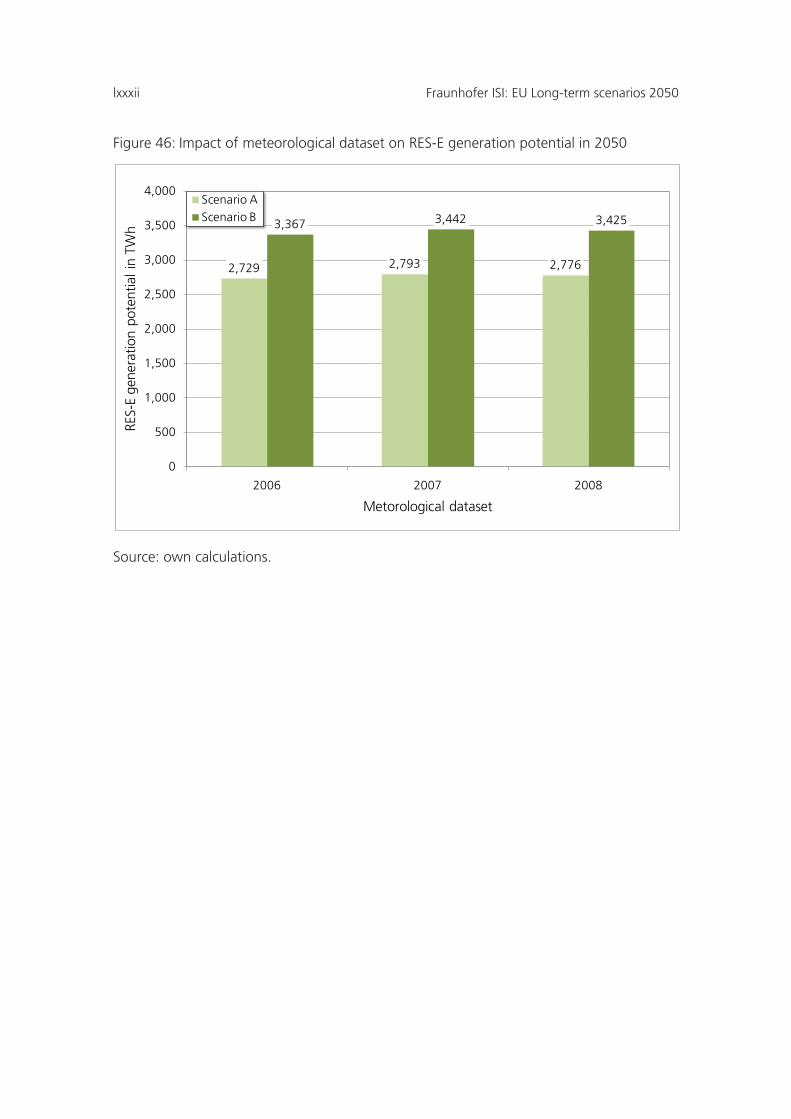
lxxxii Fraunhofer ISI: EU Long-term scenarios 2050
Figure 46: Impact of meteorological dataset on RES-E generation potential in 2050
Source: own calculations.
2,729 2,793 2,776
3,367 3,442 3,425
0
500
1,000
1,500
2,000
2,500
3,000
3,500
4,000
2006 2007 2008
RES-
E ge
nera
tion
pote
ntia
l in
TW
h
Metorological dataset
Scenario AScenario B
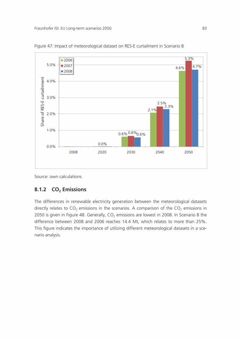
Fraunhofer ISI: EU Long-term scenarios 2050 83
Figure 47: Impact of meteorological dataset on RES-E curtailment in Scenario B
Source: own calculations.
8.1.2 CO2 Emissions
The differences in renewable electricity generation between the meteorological datasets
directly relates to CO2 emissions in the scenarios. A comparison of the CO2 emissions in
2050 is given in Figure 48. Generally, CO2 emissions are lowest in 2008. In Scenario B the
difference between 2008 and 2006 reaches 14.4 Mt, which relates to more than 25%.
This figure indicates the importance of utilizing different meteorological datasets in a sce-
nario analysis.
0.6%
2.1%
4.6%
0.0%
0.6%
2.5%
5.3%
0.6%
2.3%
4.7%
0.0%
1.0%
2.0%
3.0%
4.0%
5.0%
2008 2020 2030 2040 2050
Shar
e of
RES
-E c
urta
ilnm
ent
2006
2007
2008
lxxxiv Fraunhofer ISI: EU Long-term scenarios 2050
Figure 48: Impact of meteorological dataset on CO2 emissions in 2050
Source: own calculations.
8.1.3 Infrastructure
Other important aspects which are influenced by the meteorological dataset are the re-
quired infrastructures, such as conventional power plants, interconnectors and storage
capacity. The experience of the analysis carried out in this study shows that not only the
total RES-E generation potential is important to the results, but also its timely distribution
and correlation with electricity demand. In the analysis conducted, the biggest additions to
the interconnector capacity are necessary for the meteorological dataset of the year 2008.
In the case of Scenario A, the differences in the total interconnector capacity required for
the different meteorological dataset is between 3% and 15% for the analyzed time pe-
riod 2020 to 2050. In Scenario A the relation is comparable. A detailed comparison of the
required interconnector capacity for the different meteorological datasets is given in Table
12.
78.8
67.5 65.3
81.8
67.565.2
0
10
20
30
40
50
60
70
80
90
100
2006 2007 2008
CO
2 em
issi
ons
in M
t
Scenario A
Scenario B
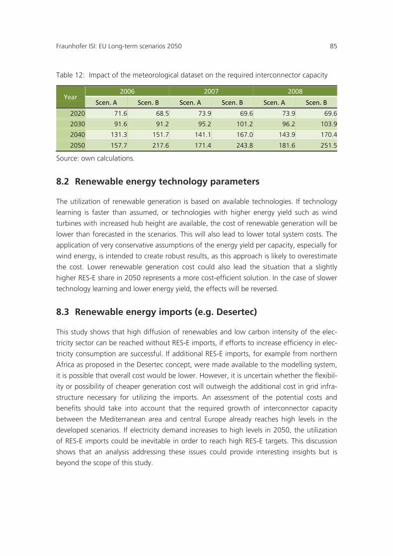
Fraunhofer ISI: EU Long-term scenarios 2050 85
Table 12: Impact of the meteorological dataset on the required interconnector capacity
Year 2006 2007 2008
Scen. A Scen. B Scen. A Scen. B Scen. A Scen. B 2020 71.6 68.5 73.9 69.6 73.9 69.6
2030 91.6 91.2 95.2 101.2 96.2 103.9
2040 131.3 151.7 141.1 167.0 143.9 170.4
2050 157.7 217.6 171.4 243.8 181.6 251.5
Source: own calculations.
8.2 Renewable energy technology parameters
The utilization of renewable generation is based on available technologies. If technology
learning is faster than assumed, or technologies with higher energy yield such as wind
turbines with increased hub height are available, the cost of renewable generation will be
lower than forecasted in the scenarios. This will also lead to lower total system costs. The
application of very conservative assumptions of the energy yield per capacity, especially for
wind energy, is intended to create robust results, as this approach is likely to overestimate
the cost. Lower renewable generation cost could also lead the situation that a slightly
higher RES-E share in 2050 represents a more cost-efficient solution. In the case of slower
technology learning and lower energy yield, the effects will be reversed.
8.3 Renewable energy imports (e.g. Desertec)
This study shows that high diffusion of renewables and low carbon intensity of the elec-
tricity sector can be reached without RES-E imports, if efforts to increase efficiency in elec-
tricity consumption are successful. If additional RES-E imports, for example from northern
Africa as proposed in the Desertec concept, were made available to the modelling system,
it is possible that overall cost would be lower. However, it is uncertain whether the flexibil-
ity or possibility of cheaper generation cost will outweigh the additional cost in grid infra-
structure necessary for utilizing the imports. An assessment of the potential costs and
benefits should take into account that the required growth of interconnector capacity
between the Mediterranean area and central Europe already reaches high levels in the
developed scenarios. If electricity demand increases to high levels in 2050, the utilization
of RES-E imports could be inevitable in order to reach high RES-E targets. This discussion
shows that an analysis addressing these issues could provide interesting insights but is
beyond the scope of this study.
lxxxvi Fraunhofer ISI: EU Long-term scenarios 2050
8.4 Availability of CCS and nuclear power
In technical terms, CCS and nuclear electricity generation are potential options for reduc-
ing CO2 emissions in the electricity sector. However, high construction costs, political un-
certainties and the unsolved problems regarding long-term nuclear waste management
render both options a risky investment. In the given scenario, both technologies are not
likely to attain adequate utilization in the case of the high penetration rates of renewables
in 2050. Depending on the actual construction costs, some CCS or nuclear capacity could
be profitable up to 2040. However, a detailed analysis with varying renewable penetration
rates and construction costs of these plant types could provide additional insights which
cannot be generated within the scope of this study.
8.5 Fuel prices
In most scenarios for the development of the electricity sector, fuel prices play a central
role in calculating the results. However, in the given scenario framework the impact of
conventional fuel prices on the results is limited. The main driver in the scenario is the CO2
cap and the development of renewable electricity generation. However, higher conven-
tional fuel prices could move the results towards a slightly higher renewable penetration,
slightly higher interconnector capacity, storage systems and vice versa. A change in the
relation between coal and gas prices could also have a slight impact on the results for the
years 2020-2030. Cheaper coal could lead to a limited increase of coal capacity in 2020 at
the cost of gas-fired units. However, the effect is likely to be limited, as coal depreciation
times are low due to the low utilization after 2030. Higher gas prices on their own could
lead to a limited shift from gas turbines to the more efficient combined cycle plants.
8.6 CO2 prices
Similar to the fuel prices, the impact of CO2 prices on the overall results is limited. It is
outweighed by the general CO2 cap for 2050. Again, the CO2 price is applied as an ex-
ogenous paramter in this study. In reality, these parameters are linked strongly. In the
given scenarios, higher CO2 prices would slightly increase the profitability of additional
RES-E generation or infrastructure in terms of interconnectors or storage systems. In the
conventional generation portfolio, higher CO2 prices shift the profitability of CO2-intensive
technologies towards less CO2 intensive technologies and vice versa. In this scenario set-
up, more electricity generation would be shifted from coal to CCGT in 2020 and 2030. In
2050 gas-fired generation would be shifted from GT to CCGT.
Fraunhofer ISI: EU Long-term scenarios 2050 87
8.7 CO2 cap
The CO2 cap in 2050 has an important impact on the results. Lowering the CO2 cap in-
creases the cost of the system. The modelling system reacts to a lower CO2 cap by higher
renewable electricity generation and more infrastructures in terms of interconnector ca-
pacity and storages. Experimental model runs show that lowering the CO2 cap while keep-
ing RES-E generation constant leads to an enormous increase in demand for storage ca-
pacity. In the case of a slightly higher CO2 cap, the costs of the system are reduced, but
the impact on the general infrastructure is moderate.
8.8 Volume of RES-E generation
The relation of RES-E generation to the CO2 cap is crucial to the results of the scenarios.
Since an integrated optimization of the power system and renewable investment is not
possible with the given resources, the adequate RES-E generation is determined by an
iterative procedure. The main procedures and results concerning the total cost of the elec-
tricity system are already described in chapter 3.1. In this section, the underlying mecha-
nisms driving the cost will be indentified. Table 13 shows the impact of a variation of the
renewable electricity generation and fixed CO2 cap on major indicators, such as storage
capacity, cost of interconnectors and RES-E curtailment. If renewable generation capacity
is reduced, the model has to reduce RES-E curtailment in order to meet the CO2 target. In
the case of ca. 40 TWh less renewable generation potential, ca. 6 GW additional storage
capacity is required. The required increase of interconnectors leads to additional costs of €
2.4 billion per year. If renewable generation is further reduced, additional storage capacity
jumps to ca. 38 GW which shows that the model is close to infeasibility.
If renewable electricity generation is increased above the selected level in the scenario,
storage capacity is also slightly increased as the possibilities for using storage capacity in-
crease. However, more than 50 % of the additional renewable generation needs to be
curtailed. These mechanisms lead to the situation that less renewable capacity leads to
higher system costs as the costs for infrastructure grows faster than the saved costs for
renewable capacity. On the other side, the costs of additional renewable generation out-
weigh the savings in infrastructure.
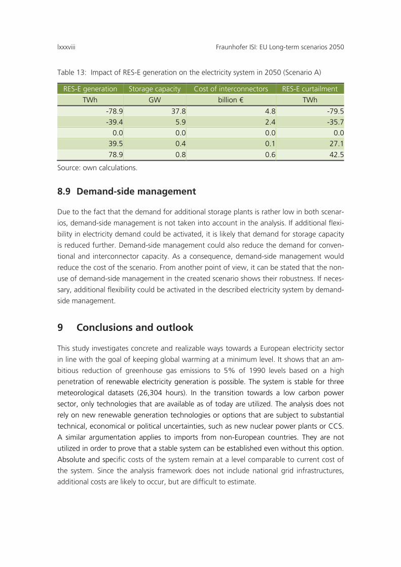
lxxxviii Fraunhofer ISI: EU Long-term scenarios 2050
Table 13: Impact of RES-E generation on the electricity system in 2050 (Scenario A)
RES-E generation Storage capacity Cost of interconnectors RES-E curtailment
TWh GW billion € TWh
-78.9 37.8 4.8 -79.5
-39.4 5.9 2.4 -35.7
0.0 0.0 0.0 0.0
39.5 0.4 0.1 27.1
78.9 0.8 0.6 42.5
Source: own calculations.
8.9 Demand-side management
Due to the fact that the demand for additional storage plants is rather low in both scenar-
ios, demand-side management is not taken into account in the analysis. If additional flexi-
bility in electricity demand could be activated, it is likely that demand for storage capacity
is reduced further. Demand-side management could also reduce the demand for conven-
tional and interconnector capacity. As a consequence, demand-side management would
reduce the cost of the scenario. From another point of view, it can be stated that the non-
use of demand-side management in the created scenario shows their robustness. If neces-
sary, additional flexibility could be activated in the described electricity system by demand-
side management.
9 Conclusions and outlook
This study investigates concrete and realizable ways towards a European electricity sector
in line with the goal of keeping global warming at a minimum level. It shows that an am-
bitious reduction of greenhouse gas emissions to 5% of 1990 levels based on a high
penetration of renewable electricity generation is possible. The system is stable for three
meteorological datasets (26,304 hours). In the transition towards a low carbon power
sector, only technologies that are available as of today are utilized. The analysis does not
rely on new renewable generation technologies or options that are subject to substantial
technical, economical or political uncertainties, such as new nuclear power plants or CCS.
A similar argumentation applies to imports from non-European countries. They are not
utilized in order to prove that a stable system can be established even without this option.
Absolute and specific costs of the system remain at a level comparable to current cost of
the system. Since the analysis framework does not include national grid infrastructures,
additional costs are likely to occur, but are difficult to estimate.
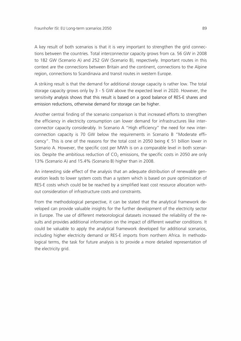
Fraunhofer ISI: EU Long-term scenarios 2050 89
A key result of both scenarios is that it is very important to strengthen the grid connec-
tions between the countries. Total interconnector capacity grows from ca. 56 GW in 2008
to 182 GW (Scenario A) and 252 GW (Scenario B), respectively. Important routes in this
context are the connections between Britain and the continent, connections to the Alpine
region, connections to Scandinavia and transit routes in western Europe.
A striking result is that the demand for additional storage capacity is rather low. The total
storage capacity grows only by 3 - 5 GW above the expected level in 2020. However, the
sensitivity analysis shows that this result is based on a good balance of RES-E shares and
emission reductions, otherwise demand for storage can be higher.
Another central finding of the scenario comparison is that increased efforts to strengthen
the efficiency in electricity consumption can lower demand for infrastructures like inter-
connector capacity considerably. In Scenario A “High efficiency” the need for new inter-
connection capacity is 70 GW below the requirements in Scenario B “Moderate effi-
ciency”. This is one of the reasons for the total cost in 2050 being € 51 billion lower in
Scenario A. However, the specific cost per MWh is on a comparable level in both scenar-
ios. Despite the ambitious reduction of CO2 emissions, the specific costs in 2050 are only
13% (Scenario A) and 15.4% (Scenario B) higher than in 2008.
An interesting side effect of the analysis that an adequate distribution of renewable gen-
eration leads to lower system costs than a system which is based on pure optimization of
RES-E costs which could be be reached by a simplified least cost resource allocation with-
out consideration of infrastructure costs and constraints.
From the methodological perspective, it can be stated that the analytical framework de-
veloped can provide valuable insights for the further development of the electricity sector
in Europe. The use of different meteorological datasets increased the reliability of the re-
sults and provides additional information on the impact of different weather conditions. It
could be valuable to apply the analytical framework developed for additional scenarios,
including higher electricity demand or RES-E imports from northern Africa. In methodo-
logical terms, the task for future analysis is to provide a more detailed representation of
the electricity grid.
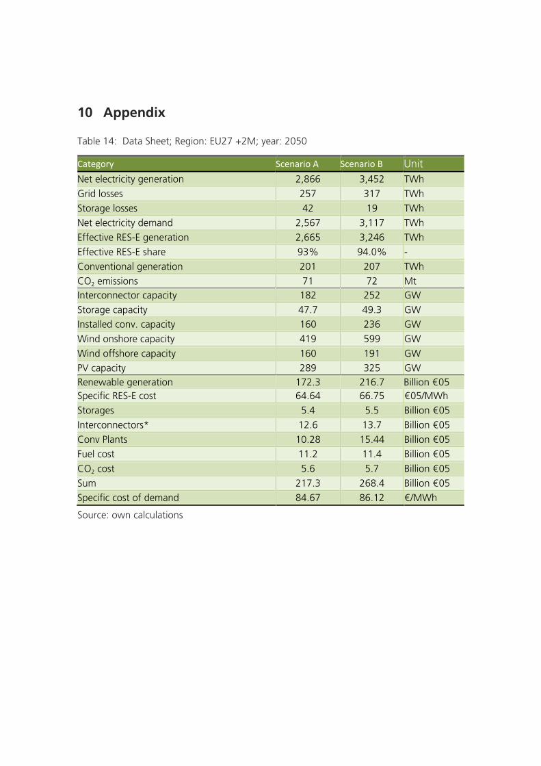
10 Appendix
Table 14: Data Sheet; Region: EU27 +2M; year: 2050
Category Scenario A Scenario B Unit Net electricity generation 2,866 3,452 TWh
Grid losses 257 317 TWh
Storage losses 42 19 TWh
Net electricity demand 2,567 3,117 TWh
Effective RES-E generation 2,665 3,246 TWh
Effective RES-E share 93% 94.0% -
Conventional generation 201 207 TWh
CO2 emissions 71 72 Mt Interconnector capacity 182 252 GW
Storage capacity 47.7 49.3 GW
Installed conv. capacity 160 236 GW
Wind onshore capacity 419 599 GW
Wind offshore capacity 160 191 GW
PV capacity 289 325 GW Renewable generation 172.3 216.7 Billion €05 Specific RES-E cost 64.64 66.75 €05/MWh
Storages 5.4 5.5 Billion €05
Interconnectors* 12.6 13.7 Billion €05
Conv Plants 10.28 15.44 Billion €05
Fuel cost 11.2 11.4 Billion €05
CO2 cost 5.6 5.7 Billion €05
Sum 217.3 268.4 Billion €05
Specific cost of demand 84.67 86.12 €/MWh
Source: own calculations
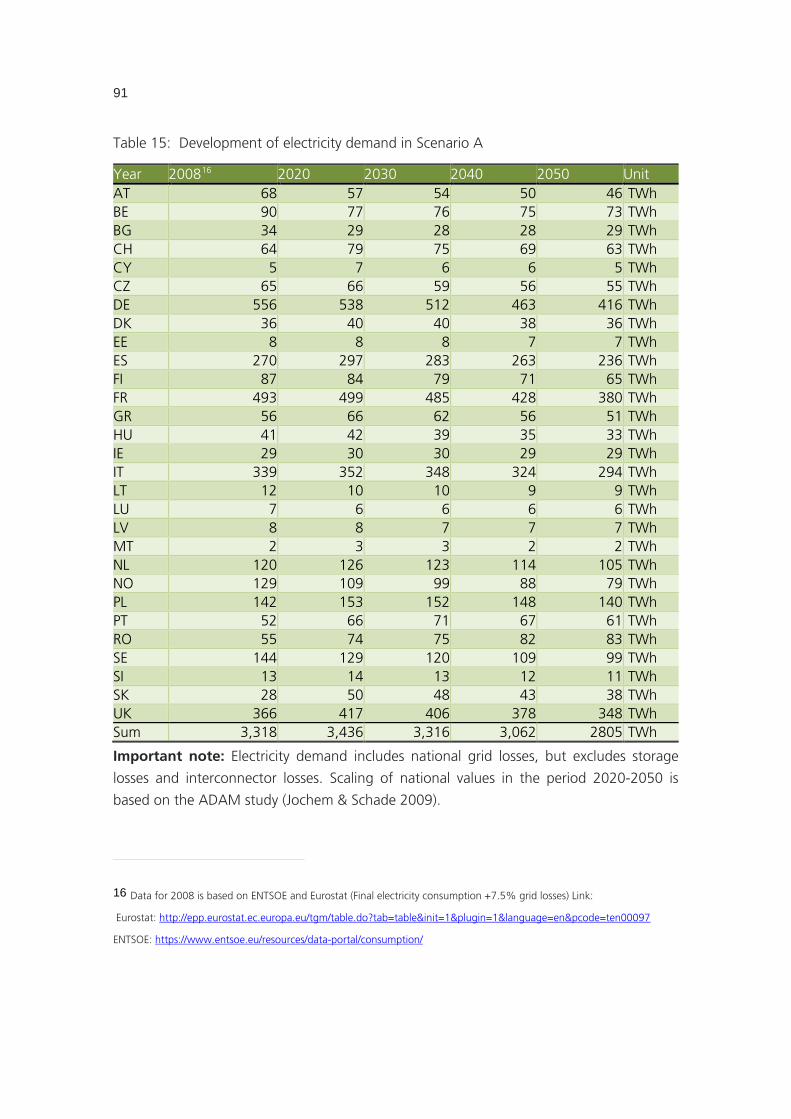
91
Table 15: Development of electricity demand in Scenario A
Year 200816 2020 2030 2040 2050 Unit AT 68 57 54 50 46 TWh BE 90 77 76 75 73 TWh BG 34 29 28 28 29 TWh CH 64 79 75 69 63 TWh CY 5 7 6 6 5 TWh CZ 65 66 59 56 55 TWh DE 556 538 512 463 416 TWh DK 36 40 40 38 36 TWh EE 8 8 8 7 7 TWh ES 270 297 283 263 236 TWh FI 87 84 79 71 65 TWh FR 493 499 485 428 380 TWh GR 56 66 62 56 51 TWh HU 41 42 39 35 33 TWh IE 29 30 30 29 29 TWh IT 339 352 348 324 294 TWh LT 12 10 10 9 9 TWh LU 7 6 6 6 6 TWh LV 8 8 7 7 7 TWh MT 2 3 3 2 2 TWh NL 120 126 123 114 105 TWh NO 129 109 99 88 79 TWh PL 142 153 152 148 140 TWh PT 52 66 71 67 61 TWh RO 55 74 75 82 83 TWh SE 144 129 120 109 99 TWh SI 13 14 13 12 11 TWh SK 28 50 48 43 38 TWh UK 366 417 406 378 348 TWh Sum 3,318 3,436 3,316 3,062 2805 TWh
Important note: Electricity demand includes national grid losses, but excludes storage
losses and interconnector losses. Scaling of national values in the period 2020-2050 is
based on the ADAM study (Jochem & Schade 2009).
16 Data for 2008 is based on ENTSOE and Eurostat (Final electricity consumption +7.5% grid losses) Link:
Eurostat: http://epp.eurostat.ec.europa.eu/tgm/table.do?tab=table&init=1&plugin=1&language=en&pcode=ten00097
ENTSOE: https://www.entsoe.eu/resources/data-portal/consumption/
Table 16: Development of electricity demand in Scenario B
Year 200817 2020 2030 2040 2050 Unit AT 68 66 66 60 49 TWh BE 90 93 91 82 67 TWh BG 34 28 29 29 27 TWh CH 64 64 61 52 39 TWh CY 5 5 5 5 5 TWh CZ 65 60 61 59 52 TWh DE 556 639 654 624 549 TWh DK 36 49 52 53 51 TWh EE 8 8 9 10 9 TWh ES 270 298 335 345 320 TWh FI 87 84 85 82 76 TWh FR 493 541 550 512 426 TWh GR 56 62 68 68 62 TWh HU 41 40 45 47 44 TWh IE 29 35 38 38 34 TWh IT 339 372 383 362 311 TWh LT 12 10 11 12 12 TWh LU 7 10 11 11 11 TWh LV 8 7 8 9 9 TWh MT 2 3 3 3 2 TWh NL 120 131 137 132 116 TWh NO 129 132 131 124 112 TWh PL 142 153 178 196 191 TWh PT 52 54 61 64 62 TWh RO 55 58 75 91 96 TWh SE 144 160 164 161 154 TWh SI 13 12 12 11 9 TWh SK 28 28 30 31 29 TWh UK 366 476 507 500 451 TWh Sum 3,318 3,677 3,861 3,774 3,376 TWh
Important note: Electricity demand includes national grid losses, but excludes storage
losses and interconnector losses. Scaling of national values is based on the TRANS-CSP
study( DLR 2006).
17 Data for 2008 is based on ENTSOE and Eurostat (Final electricity consumption +7.5% grid losses) Link:
Eurostat: http://epp.eurostat.ec.europa.eu/tgm/table.do?tab=table&init=1&plugin=1&language=en&pcode=ten00097
ENTSOE: https://www.entsoe.eu/resources/data-portal/consumption/
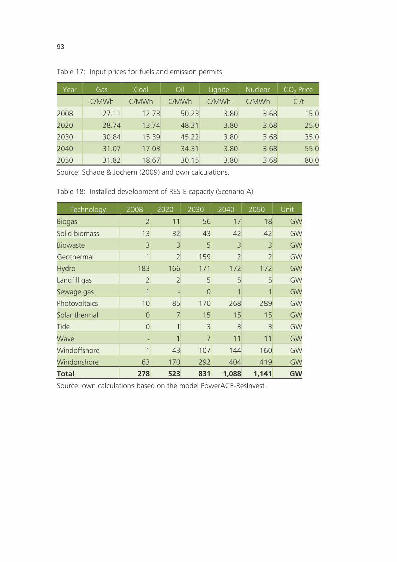
93
Table 17: Input prices for fuels and emission permits
Year Gas Coal Oil Lignite Nuclear CO2 Price
€/MWh €/MWh €/MWh €/MWh €/MWh € /t
2008 27.11 12.73 50.23 3.80 3.68 15.0
2020 28.74 13.74 48.31 3.80 3.68 25.0
2030 30.84 15.39 45.22 3.80 3.68 35.0
2040 31.07 17.03 34.31 3.80 3.68 55.0
2050 31.82 18.67 30.15 3.80 3.68 80.0
Source: Schade & Jochem (2009) and own calculations.
Table 18: Installed development of RES-E capacity (Scenario A)
Technology 2008 2020 2030 2040 2050 Unit
Biogas 2 11 56 17 18 GW
Solid biomass 13 32 43 42 42 GW
Biowaste 3 3 5 3 3 GW
Geothermal 1 2 159 2 2 GW
Hydro 183 166 171 172 172 GW
Landfill gas 2 2 5 5 5 GW
Sewage gas 1 - 0 1 1 GW
Photovoltaics 10 85 170 268 289 GW
Solar thermal 0 7 15 15 15 GW
Tide 0 1 3 3 3 GW
Wave - 1 7 11 11 GW
Windoffshore 1 43 107 144 160 GW
Windonshore 63 170 292 404 419 GW
Total 278 523 831 1,088 1,141 GW
Source: own calculations based on the model PowerACE-ResInvest.
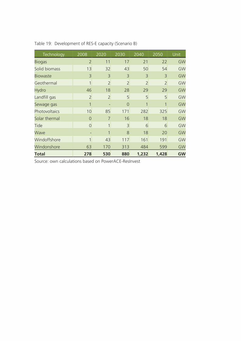
Table 19: Development of RES-E capacity (Scenario B)
Technology 2008 2020 2030 2040 2050 Unit
Biogas 2 11 17 21 22 GW
Solid biomass 13 32 43 50 54 GW
Biowaste 3 3 3 3 3 GW
Geothermal 1 2 2 2 2 GW
Hydro 46 18 28 29 29 GW
Landfill gas 2 2 5 5 5 GW
Sewage gas 1 - 0 1 1 GW
Photovoltaics 10 85 171 282 325 GW
Solar thermal 0 7 16 18 18 GW
Tide 0 1 3 6 6 GW
Wave - 1 8 18 20 GW
Windoffshore 1 43 117 161 191 GW
Windonshore 63 170 313 484 599 GW
Total 278 530 880 1,232 1,428 GW
Source: own calculations based on PowerACE-ResInvest
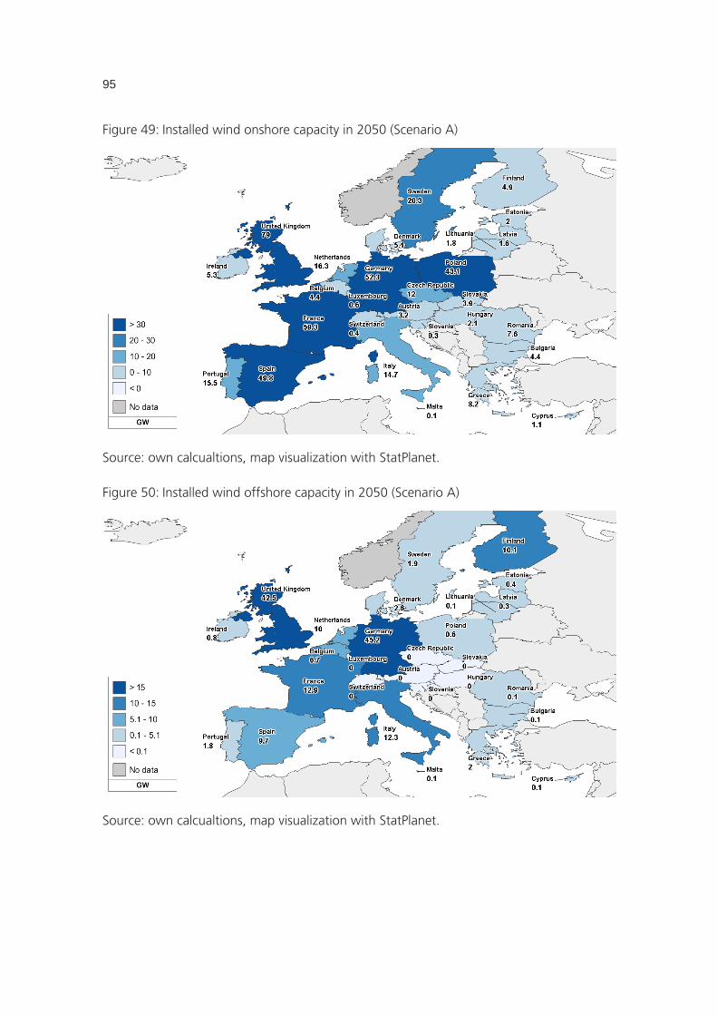
95
Figure 49: Installed wind onshore capacity in 2050 (Scenario A)
Source: own calcualtions, map visualization with StatPlanet.
Figure 50: Installed wind offshore capacity in 2050 (Scenario A)
Source: own calcualtions, map visualization with StatPlanet.
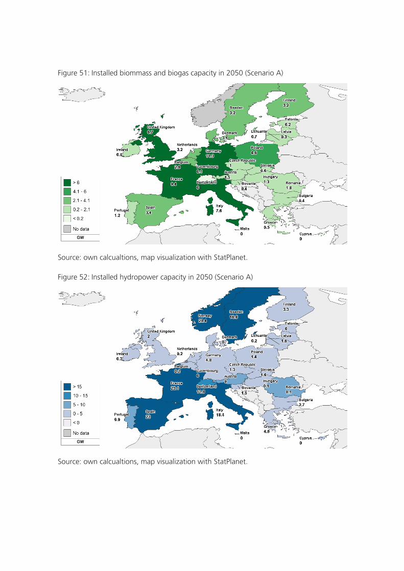
Figure 51: Installed biommass and biogas capacity in 2050 (Scenario A)
Source: own calcualtions, map visualization with StatPlanet.
Figure 52: Installed hydropower capacity in 2050 (Scenario A)
Source: own calcualtions, map visualization with StatPlanet.
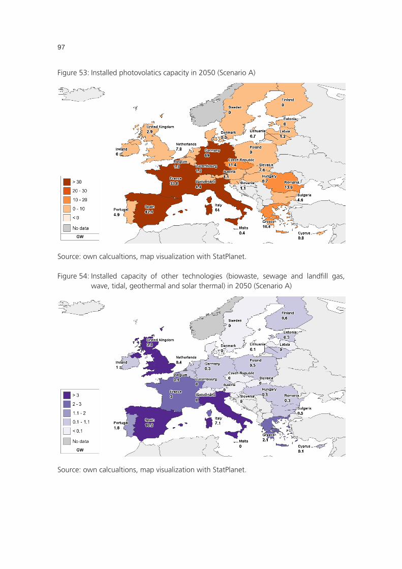
97
Figure 53: Installed photovolatics capacity in 2050 (Scenario A)
Source: own calcualtions, map visualization with StatPlanet.
Figure 54: Installed capacity of other technologies (biowaste, sewage and landfill gas, wave, tidal, geothermal and solar thermal) in 2050 (Scenario A)
Source: own calcualtions, map visualization with StatPlanet.
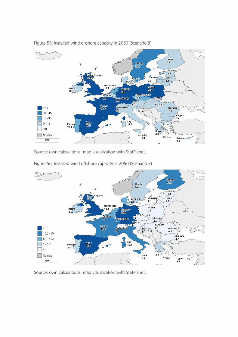
Figure 55: Installed wind onshore capacity in 2050 (Scenario B)
Source: own calcualtions, map visualization with StatPlanet.
Figure 56: Installed wind offshore capacity in 2050 (Scenario B)
Source: own calcualtions, map visualization with StatPlanet.
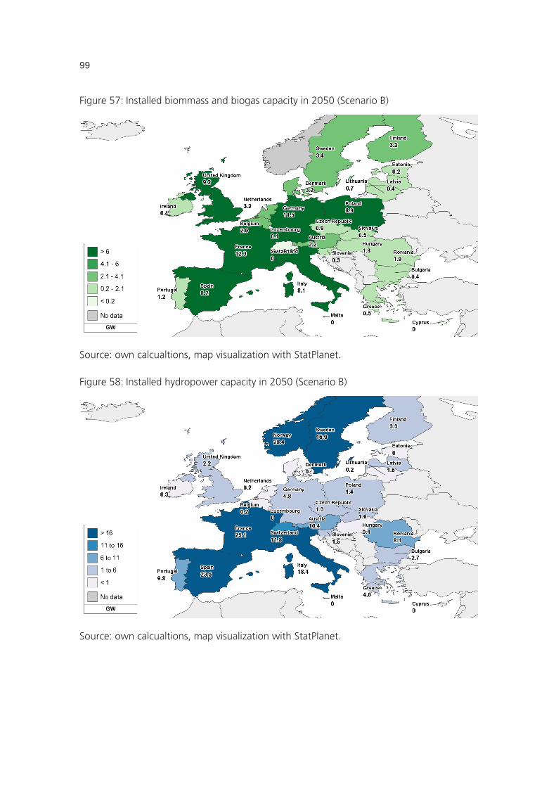
99
Figure 57: Installed biommass and biogas capacity in 2050 (Scenario B)
Source: own calcualtions, map visualization with StatPlanet.
Figure 58: Installed hydropower capacity in 2050 (Scenario B)
Source: own calcualtions, map visualization with StatPlanet.
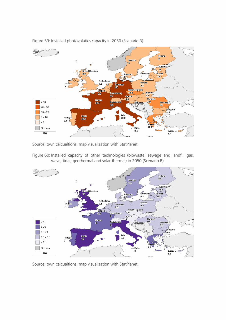
Figure 59: Installed photovolatics capacity in 2050 (Scenario B)
Source: own calcualtions, map visualization with StatPlanet.
Figure 60: Installed capacity of other technologies (biowaste, sewage and landfill gas, wave, tidal, geothermal and solar thermal) in 2050 (Scenario B)
Source: own calcualtions, map visualization with StatPlanet.
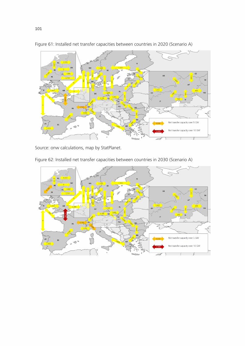
101
Figure 61: Installed net transfer capacities between countries in 2020 (Scenario A)
Source: onw calculations, map by StatPlanet.
Figure 62: Installed net transfer capacities between countries in 2030 (Scenario A)
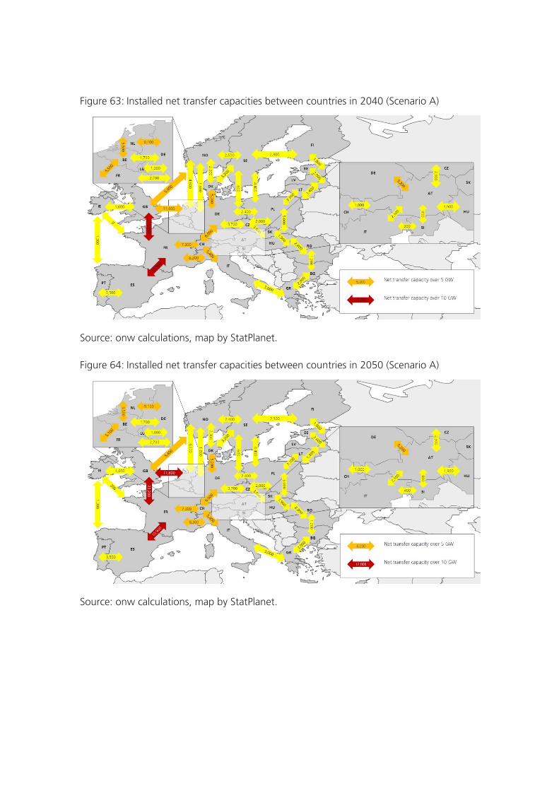
Figure 63: Installed net transfer capacities between countries in 2040 (Scenario A)
Source: onw calculations, map by StatPlanet.
Figure 64: Installed net transfer capacities between countries in 2050 (Scenario A)
Source: onw calculations, map by StatPlanet.
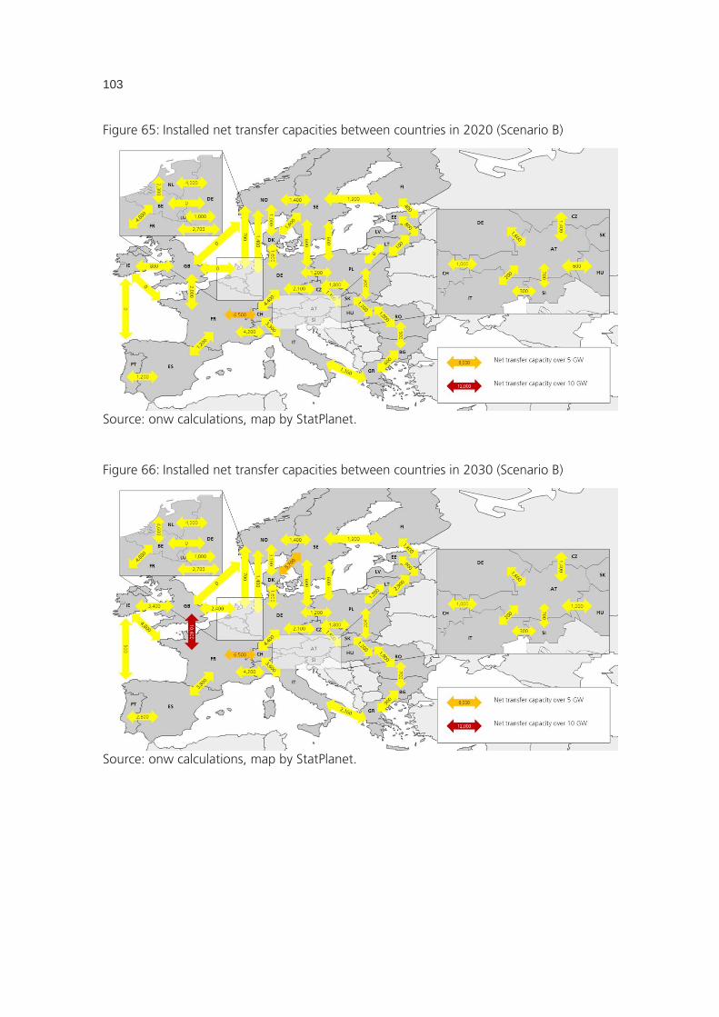
103
Figure 65: Installed net transfer capacities between countries in 2020 (Scenario B)
Source: onw calculations, map by StatPlanet.
Figure 66: Installed net transfer capacities between countries in 2030 (Scenario B)
Source: onw calculations, map by StatPlanet.
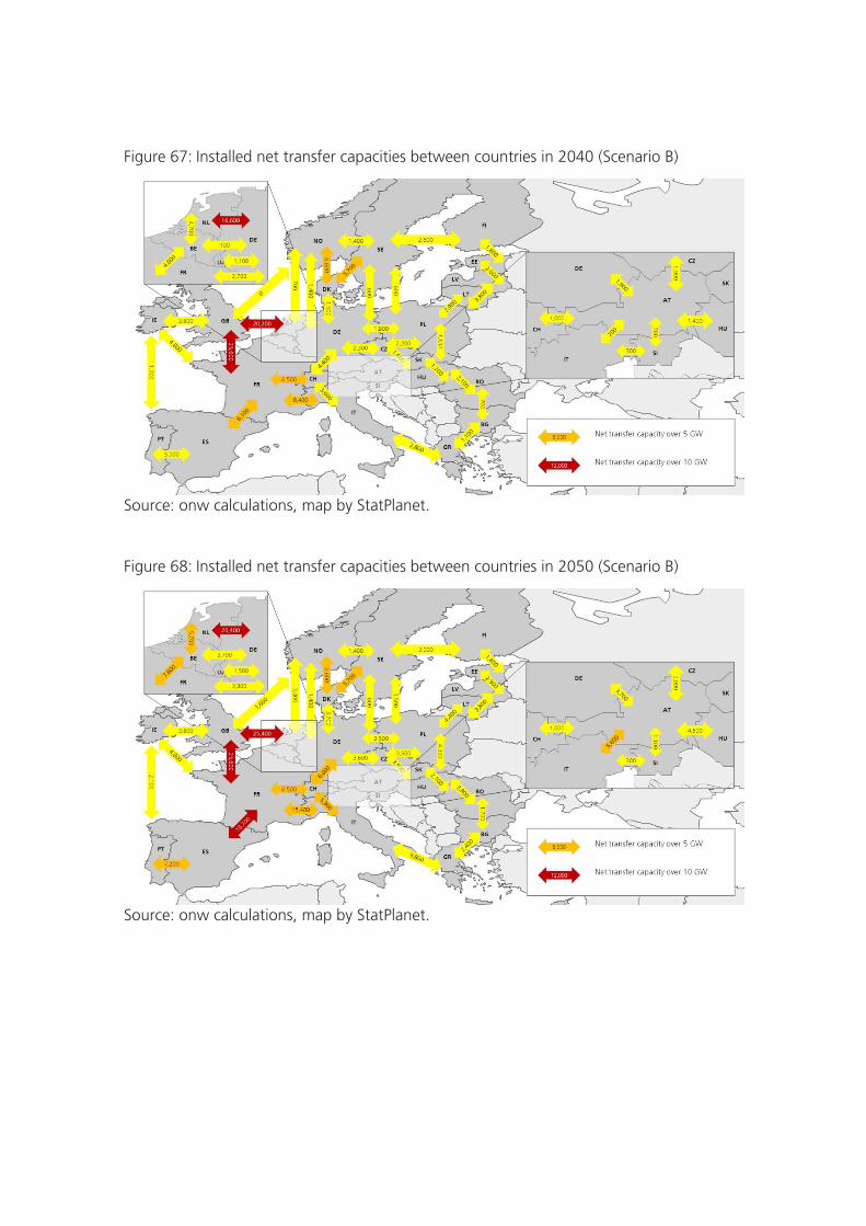
Figure 67: Installed net transfer capacities between countries in 2040 (Scenario B)
Source: onw calculations, map by StatPlanet.
Figure 68: Installed net transfer capacities between countries in 2050 (Scenario B)
Source: onw calculations, map by StatPlanet.
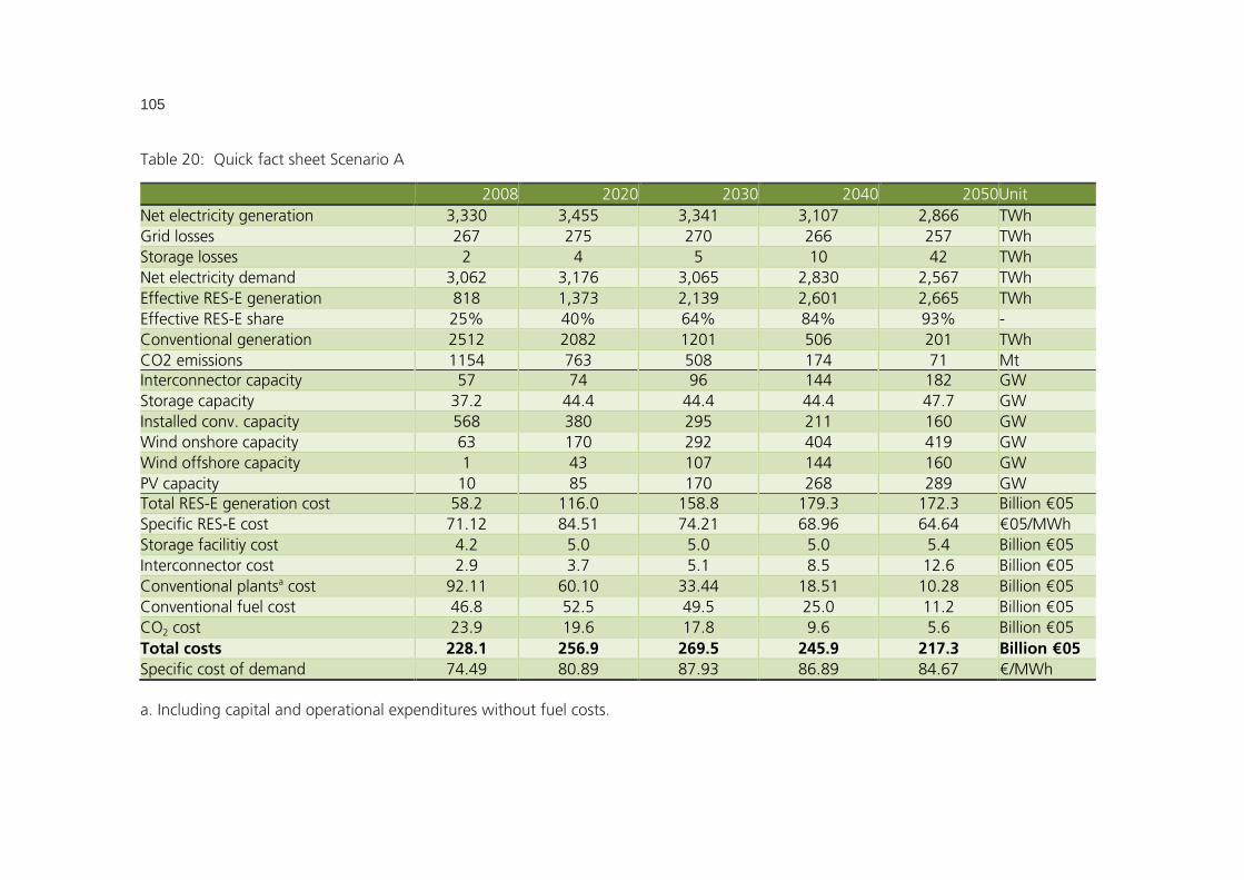
105
Table 20: Quick fact sheet Scenario A
2008 2020 2030 2040 2050 Unit Net electricity generation 3,330 3,455 3,341 3,107 2,866 TWh Grid losses 267 275 270 266 257 TWh Storage losses 2 4 5 10 42 TWh Net electricity demand 3,062 3,176 3,065 2,830 2,567 TWh Effective RES-E generation 818 1,373 2,139 2,601 2,665 TWh Effective RES-E share 25% 40% 64% 84% 93% - Conventional generation 2512 2082 1201 506 201 TWh CO2 emissions 1154 763 508 174 71 Mt Interconnector capacity 57 74 96 144 182 GW Storage capacity 37.2 44.4 44.4 44.4 47.7 GW Installed conv. capacity 568 380 295 211 160 GW Wind onshore capacity 63 170 292 404 419 GW Wind offshore capacity 1 43 107 144 160 GW PV capacity 10 85 170 268 289 GW Total RES-E generation cost 58.2 116.0 158.8 179.3 172.3 Billion €05 Specific RES-E cost 71.12 84.51 74.21 68.96 64.64 €05/MWh Storage facilitiy cost 4.2 5.0 5.0 5.0 5.4 Billion €05 Interconnector cost 2.9 3.7 5.1 8.5 12.6 Billion €05 Conventional plantsa cost 92.11 60.10 33.44 18.51 10.28 Billion €05 Conventional fuel cost 46.8 52.5 49.5 25.0 11.2 Billion €05 CO2 cost 23.9 19.6 17.8 9.6 5.6 Billion €05 Total costs 228.1 256.9 269.5 245.9 217.3 Billion €05 Specific cost of demand 74.49 80.89 87.93 86.89 84.67 €/MWh a. Including capital and operational expenditures without fuel costs.
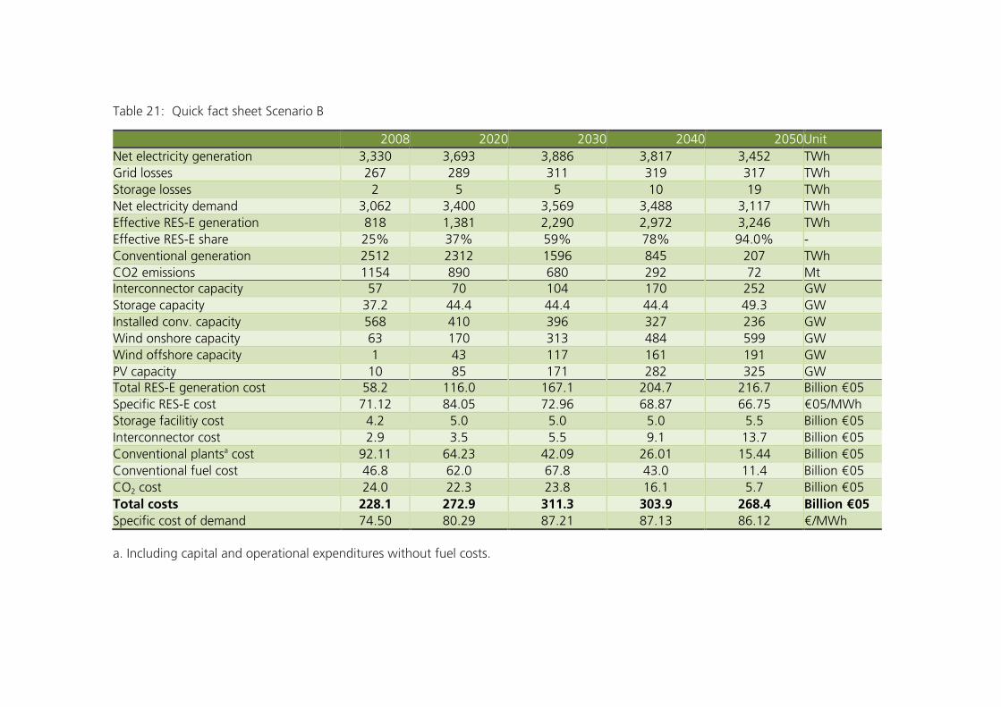
Table 21: Quick fact sheet Scenario B
2008 2020 2030 2040 2050 Unit Net electricity generation 3,330 3,693 3,886 3,817 3,452 TWh Grid losses 267 289 311 319 317 TWh Storage losses 2 5 5 10 19 TWh Net electricity demand 3,062 3,400 3,569 3,488 3,117 TWh Effective RES-E generation 818 1,381 2,290 2,972 3,246 TWh Effective RES-E share 25% 37% 59% 78% 94.0% - Conventional generation 2512 2312 1596 845 207 TWh CO2 emissions 1154 890 680 292 72 Mt Interconnector capacity 57 70 104 170 252 GW Storage capacity 37.2 44.4 44.4 44.4 49.3 GW Installed conv. capacity 568 410 396 327 236 GW Wind onshore capacity 63 170 313 484 599 GW Wind offshore capacity 1 43 117 161 191 GW PV capacity 10 85 171 282 325 GW Total RES-E generation cost 58.2 116.0 167.1 204.7 216.7 Billion €05 Specific RES-E cost 71.12 84.05 72.96 68.87 66.75 €05/MWh Storage facilitiy cost 4.2 5.0 5.0 5.0 5.5 Billion €05 Interconnector cost 2.9 3.5 5.5 9.1 13.7 Billion €05 Conventional plantsa cost 92.11 64.23 42.09 26.01 15.44 Billion €05 Conventional fuel cost 46.8 62.0 67.8 43.0 11.4 Billion €05 CO2 cost 24.0 22.3 23.8 16.1 5.7 Billion €05 Total costs 228.1 272.9 311.3 303.9 268.4 Billion €05 Specific cost of demand 74.50 80.29 87.21 87.13 86.12 €/MWh a. Including capital and operational expenditures without fuel costs.
107
11 Literature
BMU (2002). Erste Allgemeine Verwaltungsvorschrift zum Bundes-Immissionsschutzgesetz (Techni-sche Anleitung zur Reinhaltung der Luft-TA Luft). Available online: http://www.verwaltungsvorschriften-im-internet.de/bsvwvbund_24072002_IGI2501391.htm.
DLR (2006): TRANS-CSP. Trans-Mediterranean interconnection for Concentrating Solar Power. Available online: http://www.dlr.de/tt/desktopdefault.aspx/tabid-2885/4422_read-6588/.
Drews, A.; Keizer, A.C. de; Beyer, H.G.; Lorenz, E.; Betcke, J.W.H.; Sark, W.G.J.H.M. van; Heyden-reich, W.; Wiemken, E.; Stettler, S.; Toggweiler, P.; Bofinger, S.; Schneider, M.; Heilscher, G.; Heinemann, D. (2007): Monitoring and remote failure detection of grid-connected PV systems based on satellite observations. Solar Energy, 81(4), 548-564.
ECF – European Climate Foundation (2010): Roadmap 2050. A practical guide to a prosperous, low-carbon Europe. Available online: http://www.roadmap2050.eu/downloads.
ETC/LUSI, T. E. (2009): Corine land cover 2000 (CLC2000) 250 m: European Energy Agency. Avail-able online: http://www.eea.europa.eu/data-and-maps/data/corine-land-cover-2000-clc2000-250-m-version-12-2009.
ETC/LUSI, T. E. (2006). Global land cover 2000 – Europe. European Environment Agency. Available online: http://www.eea.europa.eu/data-and-maps/data/global-land-cover-2000-europe.
European Commission, (2011a). Transparency Platform - National Renewable Energy Action Plans, Database of Member States documents. Available online: http://ec.europa.eu/energy/renewables/transparency_platform/action_plan_en.htm
European Commission (2011b). Impact assessment. Accompanying document to the Communica-tion from the Commission to the European Parliament, the Council, the European Economic and Social Committee and the Committee of the Regions. A Roadmap for moving to a com-petitive low carbon economy in 2050. Available online: http://eur-lex.europa.eu/LexUriServ/LexUriServ.do?uri=SEC:2011:0288:FIN:EN:PDF.
Eurostat (2011). Databases on Energy and environment. Available online : http://epp.eurostat.ec.europa.eu/portal/page/portal/statistics/search_database.
EWEA - European Wind Energy Association (2010:) Wind in power 2009 European statistics. Avail-able online: http://www.ewea.org/fileadmin/ewea_documents/documents/statistics/ general_stats_2009.pdf.
Focken, U. (2003). Leistungsvorhersage räumlich verteilter Windkraftwanlagen unter besonderer Berücksichtigung der thermischen Schichtung der Atmosphäre. Düsseldorf: VDI.
Foken, T. (2006). Angewandte Metereologie. Mikrometeologische Methoden. Berlin: Springer.
Held (2010): Modelling the future development of renewable energy technologies in the European electricity sector using agent based simulation. Frauhofer Verlag Stuttgart.
Huld, T., Gottschalg, R. Beyer, H.G., Topic and M. (2010): Mapping the performance of PV mod-ules, effects of module type and data averaging. Solar Energy, Volume 84, Issue 2, Pages 324-338.
IPCC (2007) Climate Change 2007: Mitigation of Climate Change. Contribution of Working Group III to the Fourth Assessment Report of the Inter-governmental Panel on Climate Change, 2007. Metz, O.R. Davidson, P.R. Bosch, R. Dave, L.A. Meyer (eds). Cambridge University Press, Cam-bridge, United Kingdom and New York, NY, USA.

Kenny, R.P., Dunlop, E.D., Ossenbrink, H.A. and Müllejans, H. (2006): A practical method for the energy rating of c-Si photovoltaic modules based on standard test. Progress in: Photovoltaics: Research and Applications 14 (2006), pp. 155–166.
Nørgård and Holttinen (2004): A Multi-Turbine Power Curve Approach. In Proceedings of Nordic Wind Power Conference NWPC’04. Gothenburg, Sweden.
Rigollier, C., Lefèvre, M. and Wald, L. (2004): The method Heliosat-2 for deriving short-wave solar radiation from satellite images. Solar Energy, 77(2), p.159-169.
Schade, W. & Jochem, E. (2009): ADAM 2-degree scenario for Europe–policies and impacts. Availa-ble online: http://isi.fraunhofer.de/isi-de/n/download/publikationen/project_ADAM.pdf.
SRU - Sachverständigenrat für Umweltfragen (2010): 100 % Erneuerbare Stromversorgung bis 2050: Klimaverträglich, sicher, bezahlbar. Stellungnahme. Available online: http://www.umweltrat.de/SharedDocs/Downloads/DE/04_Stellungnahmen/2010_05_Stellung_15_erneuerbareStromversorgung.html.
Targosz, R. (2008): Network Losses. Webinar April 11, 2008. Available online: http://www.scribd.com/doc/2585592/Network-Losses.
VDI (2009): VDI 3782 Blatt 1 Umweltmeteorologie - Atmosphärische Ausbreitungsmodelle - Gauß´sches Fahnenmodell zur Bestimmung von Immissionskenngrößen.