Embed Size (px)
Citation preview
TANGENTS AND SECANTS OF ALGEBRAIC VARIETIES
F. L. Zak
Central Economics Mathematical Instituteof the Russian Academy of Sciences
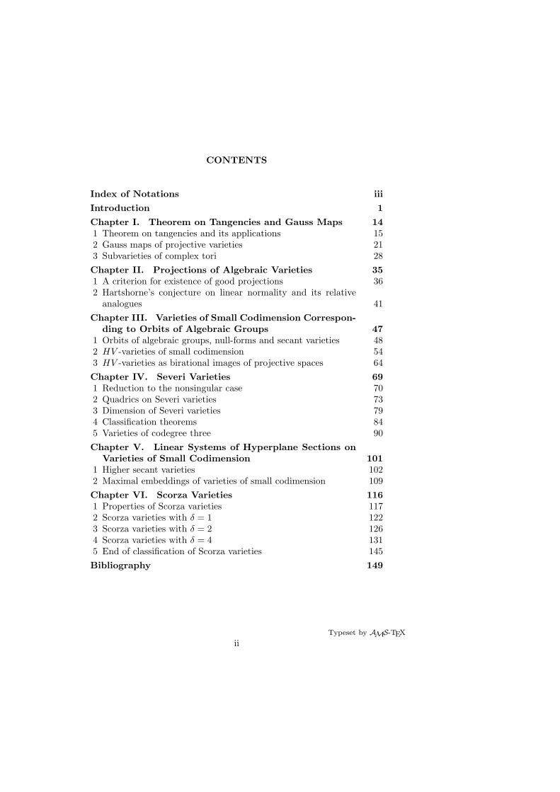
CONTENTS
Index of Notations iii
Introduction 1
Chapter I. Theorem on Tangencies and Gauss Maps 141 Theorem on tangencies and its applications 152 Gauss maps of projective varieties 213 Subvarieties of complex tori 28Chapter II. Projections of Algebraic Varieties 351 A criterion for existence of good projections 362 Hartshorne’s conjecture on linear normality and its relative
analogues 41Chapter III. Varieties of Small Codimension Correspon-
ding to Orbits of Algebraic Groups 471 Orbits of algebraic groups, null-forms and secant varieties 482 HV -varieties of small codimension 543 HV -varieties as birational images of projective spaces 64Chapter IV. Severi Varieties 691 Reduction to the nonsingular case 702 Quadrics on Severi varieties 733 Dimension of Severi varieties 794 Classification theorems 845 Varieties of codegree three 90Chapter V. Linear Systems of Hyperplane Sections on
Varieties of Small Codimension 1011 Higher secant varieties 1022 Maximal embeddings of varieties of small codimension 109Chapter VI. Scorza Varieties 1161 Properties of Scorza varieties 1172 Scorza varieties with δ = 1 1223 Scorza varieties with δ = 2 1264 Scorza varieties with δ = 4 1315 End of classification of Scorza varieties 145Bibliography 149
Typeset by AMS-TEX
ii
CHAPTER I
THEOREM ON TANGENCIES AND GAUSS MAPS
Typeset by AMS-TEX
14
1. THEOREM ON TANGENCIES AND ITS APPLICATIONS 15
1. Theorem on tangencies and its applications
Let Xn ⊂ PN be an irreducible nondegenerate (i.e. not contained in a hyper-plane) n-dimensional projective variety over an algebraically closed field K, and letY r ⊂ PN be a non-empty irreducible r-dimensional variety. We set
∆Y = (Y ×X) ∩∆X =(y, x) ∈ Y ×X
∣∣ x = y,
where ∆X is the diagonal in X ×X,
S0Y,X ⊂ (Y ×X \∆Y )× PN , S0
Y,X =(y, x, z)
∣∣ z ∈ 〈x, y〉,
where 〈x, y〉 denotes the chord joining x with y. We denote by SY,X the closure ofS0
Y,X in Y ×X×PN , by pYi the projection of SY,X onto the ith factor of Y ×X×PN
(i = 1, 2), and by ϕY : SY,X → PN the projection onto the third factor, and put
pY12 = pY
1 × pY2 : SY,X → Y ×X, S(Y, X) = ϕY (SY,X),
T ′Y,X =(pY12
)−1(∆Y ) , ψY = ϕY
∣∣T ′Y,X
, T ′(Y, X) = ψY(T ′Y,X
).
1.1. Definition. The variety S(Y, X) is called the join of Y and X or, ifY ⊂ X, the secant variety of X with respect to Y .
We observe that in the case when Y = X the above definition reduces to theusual definition of secant variety of X; we shall denote S(X,X) simply by SX.
In what follows we shall assume that Y r ⊂ Xn is a subvariety of X.
1.2. Definition. The variety T ′(Y, X) is called the variety of (relative) tangentstars of X with respect to the subvariety Y .
We observe that T ′(X,X) = T ′X is the usual variety of tangent stars (cf. [45;97]).
1.3. Definition. The cone T ′Y,X,y = ψY((
pY12
)−1 (y × y))
is called the (pro-jective) tangent star to X with respect to Y ⊂ X at a point y ∈ Y .
From this definition it is evident that T ′Y,X,y is a union of limits of chords
〈 y′, x′〉, y′ ∈ Y, x′ ∈ X, y′, x′ → y.
It is also clear that T ′Y,X,y ⊂ T ′X,y ⊂ TX,y, where T ′X,y = T ′X,X,y is the (projective)tangent star to X at y (cf. [45; 97]) and TX,y is the (embedded) tangent space toX at y. On the other hand, T ′Y,X,y ⊃ T ′y,X , where T ′y,X = T ′y,X,y is the (projective)tangent cone to X at the point y.
By definition, T ′(Y, X) = ∪y∈Y
T ′Y,X,y. If X is nonsingular along Y , i.e. Y ∩Sing X = ∅ and Y ⊂ Sm X = X \ Sing X, then T ′(Y, X) = T (Y, X) = ∪
y∈YTX,y is
the usual variety of tangents.
16 I. THEOREM ON TANGENCIES AND GAUSS MAPS
1.4. Theorem. An arbitrary irreducible subvariety Y r ⊂ Xn, r ≥ 0 satisfiesone of the following two conditions:
a) dim T ′(Y,X) = r + n, dim S(Y,X) = r + n + 1;b) T ′(Y,X) = S(Y, X).
Proof. Let t = dim T ′(Y,X). It is clear that t ≤ r+n. In the case when t = r+nthe theorem is obvious since S(Y, X) is an irreducible variety, S(Y, X) ⊃ T ′(Y,X)and dim S(Y, X) ≤ r + n + 1.
Suppose that t < r + n, and let LN−t−1 be a linear subspace of PN such that
L ∩ T ′(Y,X) = ∅. (1.4.1)
We denote by π:PN \ L → Pt the projection with center at L and put X ′ = π(X),Y ′ = π(Y ). Since π
∣∣X
is a finite morphism, we have dim (Y ′×X ′) = r + n > t,
and from the connectedness theorem of Fulton and Hansen (cf. [26] and [27, 3.1])it follows that
Y ×X′X =(π∣∣Y×π
∣∣X
)−1 (∆Pt)
is a connected scheme.I claim that
Supp (Y ×X′X) = ∆Y . (1.4.2)
In fact, suppose that this is not so. Then by definition for all (y, x) ∈ (Y ×X′X)\∆Y
we haveϕY
((pY12
)−1(y, x)
)∩ L 6= ∅,
and therefore for each point (y, y) ∈ ∆Y ∩ ((Y ×X′X) \∆Y )
T ′(Y,X) ∩ L ⊃ T ′Y,X,y ∩ L = ϕY((
pY12
)−1(y, y)
)∩ L 6= ∅
contrary to (1.4.1). This proves (1.4.2).From (1.4.2) it follows that L ∩ S(Y,X) = ∅. Hence
t ≤ dim S(Y, X) ≤ N − dim L− 1 = t,
i.e. condition b) holds. ¤
1.5. Corollary. codimS(Y,X) T ′(Y, X) ≤ 1.
1.6. Definition. Let L ⊂ PN be a linear subspace. We say that L is tangentto a variety X ⊂ PN along a subvariety Y ⊂ X (resp. L is J-tangent to X alongY , resp. L is J-tangent to X with respect to Y ) if L ⊃ TX,y (resp. L ⊃ T ′X,y, resp.L ⊃ T ′Y,X,y) for all points y ∈ Y .
It is clear that if L is tangent to X along Y , then L is J-tangent to X along Yand if L is J-tangent to X along Y , then L is J-tangent to X with respect to Y .If X is nonsingular along Y , then all the three notions are identical.
1. THEOREM ON TANGENCIES AND ITS APPLICATIONS 17
1.7. Theorem. Let Y r ⊂ Xn and Zb ⊂ Y r be closed subvarieties, and letLm ⊂ PN , n ≤ m ≤ N−1 be a linear subspace which is J-tangent to X with respectto Y along Y \Z (i.e. L ⊃ T ′Y,X,y for all points y ∈ Y \Z). Then r ≤ m−n+ b+1.
Proof. It is clear that Theorem 1.7 is true (and meaningless) for r ≤ b + 1.Suppose that r > b + 1. Without loss of generality we may assume that Y isirreducible. Let M be a general linear subspace of codimension b + 1 in PN . Put
X ′ = X ∩M, Y ′ = Y ∩M, L′ = L ∩M.
It is clear thatn′ = dim X ′ = n− b− 1,
r′ = dim Y ′ = r − b− 1,
m′ = dim L′ = m− b− 1
(1.7.1)
and L′ is J-tangent to X ′ with respect to Y ′ along Y ′. In other words,
T ′(Y ′, X ′) ⊂ L′. (1.7.2)
In particular, from (1.7.2) it follows that
dim T ′(Y ′, X ′) ≤ m′. (1.7.3)
Since n > r > b+1, from the Bertini theorem it follows that the varieties X ′ and Y ′
are irreducible. By [58, Lema 1, Corolario 1], the variety X ′ is nondegenerate, andso the relative secant variety S(Y ′, X ′) containing X ′ does not lie in the subspaceL′. From (1.7.2) it follows that
S(Y ′, X ′) 6= T ′(Y ′, X ′). (1.7.4)
In view of (1.7.4) Theorem 1.4 yields
dim T ′(Y ′, X ′) = r′ + n′. (1.7.5)
Combining (1.7.3) and (1.7.5) we see that r′ + n′ ≤ m′, and in view of (1.7.1)r ≤ m− n + b + 1. ¤
1.8. Corollary (Theorem on tangencies). If a linear subspace Lm ⊂ PN istangent to a nondegenerate variety Xn ⊂ PN along a closed subvariety Y r ⊂ Xn,then r ≤ m− n.
1.9. Remark. It is clear that if Z does not contain components of Y , then inthe statement of Theorem 1.7 we may assume that Z ⊂ Y ∩ Sing X.
We give an example showing that the bound in Theorem 1.7 is sharp.
1.10. Example. Let Xn ⊂ PN , N = 2n− b− 2 be a cone with vertex Pb overthe Segre variety P1 × Pn−b−2 ⊂ P2n−2b−3, n > b + 2. Then
X∗ = (X ′)∗ = P1 × Pn−b−2 ⊂ (Pb)∗ = P2n−2b−3,
18 I. THEOREM ON TANGENCIES AND GAUSS MAPS
and a subspace Lm ⊂ PN , n ≤ m ≤ N − 1 is tangent to X at a point x ∈ SmX(and all points of the (b+1)-dimensional affine linear space 〈x,Pb〉 \Pb) if and onlyif the (N −m− 1)-dimensional linear subspace L∗ is contained in the (N − n− 1)-dimensional linear subspace T ∗X,x ⊂ X∗ (here and in what follows asterisk denotesdual variety and 〈A〉 denotes the linear span of a subset A ⊂ PN ). It is easy tosee that an arbitrary (n− b− 3)-dimensional linear subspace lying in X∗ coincideswith T ∗X,x for some x ∈ X.
LetPn−b−2 ⊂ X∗ = P1 × Pn−b−2
be a linear subspace, and let L∗ be an arbitrary (N − m − 1)-dimensional linearsubspace of Pn−b−2. Then the m-dimensional linear subspace L = (L∗)∗ is tangentto X at all points of Y \ Pb, where
Y = Pm−n+b+1 ⊃ Pb, Y =x ∈ X
∣∣ L∗ ⊂ T ∗X,x ⊂ Pn−b−2.
Thus for the subspace L and the subvarieties Y = Pm−n+b+1 ⊂ Pn−1 ⊂ X andZ = Sing X = Pb the inequality in Theorem 1.7 turns into equality.
1.11. Proposition. Let Xn ⊂ PN be a nondegenerate variety satisfyingcondition Rk (cf. [30, Chapter IV2, (5.8.2)]) (in other words, X is regular incodimension k, i.e. b = dim (Sing X) < n − k), and let L be an m-dimensionallinear subspace of PN . Put X ′ = X · L, and let b′ = dim (Sing X ′). Thenb′ ≤ 2N −m−n+ b−1 = b+ c+ ε−1, i.e. X ′ satisfies condition Rk−c−2ε+1, wherec = codimPN X = N − n, ε = codimPN L = N −m.
Proof. For an arbitrary point λ of the (ε− 1)-dimensional linear subspace L∗ ⊂PN∗ we put Xλ = X ·λ∗, where λ∗ is the hyperplane corresponding to λ. It is clearthat X ′ = ∩
λ∈L∗Xλ. Let Y = Sing X ′, Yλ = Sing Xλ, λ ∈ L∗. It is easy to see that
Y ⊂ ∪λ∈L∗
Yλ, so that
b′ = dim Y ≤ maxλ∈L∗
bλ + ε− 1, (1.11.1)
where bλ = dim Yλ. It is clear that the hyperplane λ∗ is tangent to X at all pointsof Yλ \ Sing X. Hence from Theorem 1.7 it follows that
bλ ≤ b + c. (1.11.2)
Combining (1.11.1) and (1.11.2) we obtain the desired bound for b′. ¤The following simple example shows that the bound in Proposition 1.11 is sharp.
1.12. Example. Let XN−1 ⊂ PN be a quadratic cone with vertex Pb, andlet
[N+b
2
]+ 1 ≤ m ≤ N − 1 (here and in what follows [a] is the largest integer
not exceeding a given number a ∈ R). Then X∗ is a nonsingular quadric in the(N − b − 1)-dimensional linear subspace (Pb)∗ ⊂ PN∗. It is well known (cf. [28,Volume II, Chapter 6; 37, Chapter XIII]) that X∗ contains a linear subspace ofdimension
[N−b−2
2
]. Let L∗ be its linear subspace of dimension N −m − 1. Put
L = (L∗)∗, X ′ = X · L. Then dimL = m, and it is easy to see that Y = Sing X ′ isan (N −m + b)-dimensional linear subspace.
1. THEOREM ON TANGENCIES AND ITS APPLICATIONS 19
1.13. Corollary. Suppose that a variety Xn ⊂ PN satisfies conditions Sε+1 =SN−m+1 and Rc+2ε−1 = R3N−2m−n−1, and let Lm ⊂ PN be a linear subspace forwhich dim (X · L) = n − ε = m + n − N . Then the scheme X · L is reduced. Inparticular, if X is nonsingular, N < 2
3 (m + n + 1), and dim X · L = m + n − N ,then X · L is a reduced scheme.
Proof. From Proposition 1.11 it follows that in the conditions of Corollary 1.13X ′ = X · L satisfies condition R0. Since dim X ′ = n− ε, X ′ satisfies condition S1
(cf. [61,§ 17]). Hence to prove Corollary 1.13 it suffices to apply Proposition 5.8.5from [30, Chapter IV2]. ¤
1.14. Corollary. If Xn ⊂ PN satisfies conditions Sε+2 = SN−m+2 and Rc+2ε =R3N−2m−n and Lm ⊂ PN is a linear subspace such that dim (Xn · Lm) = n − ε =m+n−N , then the scheme X ·L is normal (and therefore irreducible and reduced).In particular, if X is nonsingular, N ≤ 2
3 (m + n) and dim (X · L) = m + n − N ,then X · L is a normal scheme.
Proof. From Proposition 1.11 it follows that in the conditions of Corollary 1.14X ′ = X · L satisfies condition R1. Since dim X ′ = n− ε, X ′ satisfies condition S2
(cf. [61,§ 17]). Hence to prove Corollary 1.14 it suffices to apply Serre’s normalitycriterion (cf. [30, Chapter IV2, (5.8.6)]). ¤
Of special importance to applications is the case when L is a hyperplane. Weformulate our results in this case.
1.15. Corollary. a) If a variety Xn ⊂ PN is nondegenerate and normal andN ≤ 2n − b − 1, where b = dim (Sing X), then all hyperplane section ofX are reduced. In particular, if X is nonsingular and N < 2n, then allhyperplane sections of X are reduced.
b) If a nondegenerate variety Xn ⊂ PN has properties S3 and RN−n+2 (thelast assumption means that N < 2n− b− 2), then all hyperplane sectionsof X are normal (and therefore irreducible and reduced). In particular, ifX is nonsingular and N < 2n − 1, then all hyperplane sections of X arenormal.
1.16. Remark. Corollary 1.15 gives a much more precise information thanBertini type theorems describing properties of generic hyperplane sections (cf. e.g.[80]), but, as shown by Examples 1.18 and 1.19 below, the assumptions in its state-ment cannot be weakened.
1.17. Remark. If K = C and b = −1, then in the assumptions of Corol-lary 1.15 b) irreducibility of hyperplane sections follows from the Barth-Larsen the-orem according to which for N < 2n− 1 the Picard group Pic X ' Z is generatedby the class of hyperplane section of X (cf. [54; 60; 65]).
We give examples showing that the bounds in Corollary 1.15 are sharp.
1.18. Example. Let X0 = P1 × Pn−b−1 ⊂ P2n−2b−1, n > b + 1, and letY0 = x × Pn−b−2 ⊂ X0 be a linear subspace. We denote by X ′ ⊂ P2(n−b−1)
the section of X0 by a general hyperplane passing through Y0. It is easy to seethat X ′ is a nonsingular projectively normal variety (cf. e.g. [73]). Let Xn ⊂ PN
20 I. THEOREM ON TANGENCIES AND GAUSS MAPS
, N = 2n − b − 1 be the projective cone with vertex Pb over X ′. It is clear thatX is a normal variety and dim (Sing X) = b, so that X satisfies conditions S2 andRn−b−1 = RN−n. However X has a non-reduced hyperplane section correspondingto the hyperplane in P2n−2b−1 which is tangent to X0 along Y0 (cf. Example 1.10).
1.19. Example. Let X0 = Pn−b−2 ⊂ P2n−2b−3, n > b + 2, and let X be theprojective cone with vertex Pb over X0. Then Xn ⊂ PN , N = 2n − b − 2 is aCohen-Macaulay variety (cf. e.g. [47; 73]) and dim (Sing X) = b, so that X satisfiesconditions S3 and Rn−b−1 = RN−n+1. However for each hyperplane L such thatL∗ ∈ X∗ = X∗
0 L ·X is a reducible and therefore non-normal variety, viz. L ·X =H1 ∪H2, where H1 = Pn−1 and H2 is the cone with vertex Pb over P1 × Pn−b−3, isa reducible and therefore non-normal variety, and Sing (L ·X) = H1 ∩H2 = Pn−2
(cf. Example 1.10).
2. GAUSS MAPS OF PROJECTIVE VARIETIES 21
2. Gauss maps of projective varieties
Let Xn ⊂ PN be an irreducible nondegenerate variety. For n ≤ m ≤ N − 1 weput
Pm =(x, α) ∈ SmX ×G(N, m)
∣∣ Lα ⊃ TX,x
,
where G(N, m) is the Grassmann variety of m-dimensional linear subspaces in PN ,Lα is the linear subspace corresponding to a point α ∈ G(N, m), and the bar denotesclosure in X × G(N, m). We denote by pm : Pm → X (resp. γm : Pm → G(N, m))the projection map to the first (resp. second) factor.
2.1. Definition. The map γm is called the mth Gauss map, and its imageX∗
m = γm(Pm) is called the variety of m-dimensional tangent subspaces to thevariety X.
2.2. Remark. Of special interest are the two extreme cases, viz. m = n andm = N − 1. For m = n we get the ordinary Gauss map γ : X 99K G(N,n), andfor m = N − 1 we see that X∗
N−1 = X∗ ⊂ PN is the dual variety and if X isnonsingular, then PN−1
N−1 = P(NPN /Xn(−1)
), where NPN /Xn is the normal bundle
to X in PN (cf. [16, Expose XVII]).
2.3. Theorem. Let dim (Sing X) = b ≥ −1. Then
a ) for each point α ∈ γm
(p−1
m (SmX)), dim γ−1
m (α) ≤ m− n + b + 1;a′) dim X∗
m ≥ (m− n)(N −m− 2) + (m− b− 1);b ) for a general point α ∈ X∗
m, dim γ−1m (α) ≤ max
b + 1, m + n−N − 1
;
b′) dim X∗m ≥ min
(m− n)(N −m) + n− b− 1, (m− n + 1)(N −m) + 1
;
c ) if charK = 0 and γm = νmγm is the Stein factorization of the mor-phism γm, then νm is a birational isomorphism and the generic fiber of themorphism γm (and γm) is a linear subspace of PN of dimension dimPm −dim X∗
m.
Proof. a) immediately follows from Theorem 1.7, and since
dimPm = dim X + dim G(N − n− 1,m− n− 1)
= n + (m− n)(N −m), (2.3.1)
a′) follows from a).b) Suppose first that m = N − 1. It is clear that dim γ−1
N−1(α) ≤ n − 1, and itsuffices to verify that if n−1 ≥ b+2, i.e. n ≥ b+3, then for a general point α ∈ X∗
we have dim γ−1N−1(α) 6= n − 1. Suppose that this is not so, and let x be a general
point of X. Since n − 1 > b + 1, from Theorem 1.7 it follows that the system ofdivisors
Yα = pN−1
(γ−1
N−1(α)), α ∈ T ∗X,x
is not fixed, and therefore X = ∪αYα, where α runs through the set of general points
of T ∗X,x. Hence for a general point y ∈ X there exists a hyperplane Λy ⊂ T ∗X,x suchthat for a general point β ∈ Λy we have Lβ ⊃ TX,y. But then
〈TX,x, TX,y〉 ⊂ (Λy)∗ = Pn+1,
22 I. THEOREM ON TANGENCIES AND GAUSS MAPS
i.e. for a general pair of points x, y ∈ X we have
dim (TX,x ∩ TX,y) = n− 1.
From this it follows that either all n-dimensional linear subspaces from γn(X) arecontained in an (n + 1)-dimensional linear subspace Pn+1 ⊂ PN or they all passthrough an (n − 1)-dimensional subspace Pn−1 ⊂ PN . But in the first case Xis a hypersurface and by Theorem 1.7 dim Yα = n − 1 ≤ b + 1, contrary to ourassumption, and in the second case the intersection of X with a general linearsubspace PN−n+1⊂ PN is a nonsingular strange curve (we recall that a projectivecurve of degree ≥ 2 is called strange if all its tangent lines pass through a fixedpoint). It is well known (cf. [59; 34, ChapterIV; 39 or 75]) that the only nonsingularstrange curves are conics in characteristic 2. Therefore in the second case X isa quadric, and we again come to a contradiction. Thus assertion b) holds form = N − 1 (if charK = 0, then one can simplify the proof using the reflexivitytheorem according to which (X∗)∗ = X (cf. [96])).
Next we prove assertion b) for m = k under the assumption that it holds form = k + 1. It is clear that for general points αk ∈ X∗
k , αk+1∈ X∗k+1 we have
dim Yαk≤ dim Yαk+1 . (2.3.2)
If b + 1 ≥ k + n−N , then from the induction hypothesis it follows that
dim Yαk≤ dim Yαk+1 ≤ b + 1.
Suppose thatdim Yαk+1 ≤ k + n−N > b + 1. (2.3.3)
If dimYαk< dim Yαk+1 , then assertion b) for m = k immediately follows from
(2.3.3). Otherwise from (2.3.2) and (2.3.3) it follows that for a general point x ∈ Xand a general point αk+1 ∈ X∗
k+1 for which Yαk+1 3 x each hyperplane in Lαk+1
containing TX,x is tangent to X at all points of a (dim Yαk+1)-dimensional compo-nent of Yαk+1 that are nonsingular on X, and by Theorem 1.7 dim Yαk+1 ≤ b + 1.But then
dim Yαk= dim Yαk+1 ≤ b + 1,
so that inequality b) holds also in this case. Assertion b) is proved.b′) immediately follows from b) in view of (2.3.1).c) Let αm be a general point of X∗
m. The linear subspace Lmαm⊂ PN is tangent
to X at all points of the subvariety
Yαm∩ SmX, Yαm = pm
(γ−1
m (αm)),
and it is easy to see that
Yαm ∩ SmX =⋂
Lα⊃Lαm
(Yα ∩ SmX
), (2.3.4)
2. GAUSS MAPS OF PROJECTIVE VARIETIES 23
where α runs through the set of points of X∗ for which Lα ⊃ Lαm. From the
reflexivity theorem (cf. e.g. [49]) it follows that if charK = 0, then for a generalpoint α ∈ X∗ we have
Yα = pN−1
(γ−1
N−1 (α))
= (TX∗,α)∗ (2.3.5)
is a linear subspace of PN of dimension N − dim X∗ − 1. From (2.3.4) and (2.3.5)it follows that
Yαm= Yαm
∩ SmX =⋂
Lα⊃Lαm
(TX∗,α)∗
is also a linear subspace of PN . Since charK = 0, the morphism γm is separableand therefore smooth at a general point. Hence νm is a birational isomorphism.This completes the proof of assertion c) and Theorem 2.3. ¤
We observe that if charK = p > 0, then assertion c) of Theorem 2.3 is no longertrue. As an example, it suffices to consider the hypersurface in Pn+1 defined by
equationn+1∑i=0
xp+1i = 0 (in this case γ is the Frobenius map). The case of positive
characteristic is treated in [50].
2.4. Corollary. If charK = 0, Xn ⊂ PN is a nonsingular variety, and N −n + 1 ≤ m ≤ N − 1, then a general m-dimensional tangent subspace is tangent toX along a linear subspace of dimension at most m + n − N − 1 (for N ≥ 2n thisbound is better than the one given in Theorem 1.7). For n ≤ m ≤ N − n + 1 ageneral m-dimensional tangent subspace is tangent to X at a single point.
2.5. Corollary. Let Xn ⊂ PN , Xn 6= Pn, n∗ = dim X∗, b = dim (Sing X).Then n∗ ≥ n− b− 1. In particular, for a nonsingular variety n∗ ≥ n. If n ≥ b + 3,then n ≥ N −n+1 (this bound is better than the preceding one if N ≥ 2n− b−1).
The following example shows that both bounds in Corollary 2.5 are sharp.
2.6. Example. Let X0 = P1 × Pn−b−2 ⊂ P2n−2b−3, n > b + 2, and let X bea projective cone with vertex Pb and base X0. Then Xn ⊂ PN , N = 2n − b − 2,dim (Sing X) = b, X∗ = X∗
0 ' X0, and n∗ = n− b− 1 = N − n + 1.
2.7. Remark. In the case when charK = 0 and b = −1, the inequality n∗ ≥N − n + 1 was independently proved by Landman (cf. [50]). Another proof wasearlier given by the author (cf. [96, Proposition 1] for n = 2; the general case isquite similar).
2.8. Corollary. Let Xn ⊂ PN , Xn 6= Pn, b = dim (Sing X). Then dim γ(X) ≥n − b − 1. In particular, for a nonsingular variety, dim γ(X) = dim X and γ is afinite morphism. If in addition charK = 0, then γ is a birational isomorphism (i.e.γ is the normalization morphism).
2.9. Remark. In the case when K = C and b = −1, Griffiths and Harris [29]proved that dim γn(X) = dim X. Different proofs of finiteness of γn in this casewere later given by Ein [18] and Ran [68]. In our first proof of Corollary 2.8 (andTheorem 1.7) we used methods of formal geometry. Since related techniques is usedin §3, we give this proof here.
24 I. THEOREM ON TANGENCIES AND GAUSS MAPS
As in the proof of Theorem 1.7, considering the intersection of X with a general(N−b−1)-dimensional linear subspace of PN we reduce everything to the case whenb = −1. Suppose that the n-dimensional linear subspace L corresponding to a pointαL ∈ G(N,n) is tangent to X along an irreducible subvariety Y , dim Y > 0, i.e.Y ⊂ γ−1(αL). Let X = X/Y be the completion of X along Y , and let G = γ(X)/αL
be the formal neighborhood of the point αL in the variety γ(X) ⊂ G(N, n). SinceXn 6= Pn, dim γ(X) > 0. Hence H0(G,OG) and H0(X,OX) ⊃ H0(G,OG) areinfinite-dimensional vector spaces over the field K.
On the other hand, let M ⊂ PN be a linear subspace, dim M = N − n − 1,M ∩ L = ∅, and let π : X 99K Pn be the projection with center at M . Thenπ/Y : X → Pn
/π(Y ) is an isomorphism of formal spaces, and therefore
H0 (X,OX) ' H0(L,OL) , (2.9.1)
where L = L/Y ' Pn/π(Y ) is the completion of L along Y . But by the well-known
theorem on formal functions (cf. [31, Chapter V; 36]), H0(L,OL) = K which isimpossible since H0 (X,OX) is infinite-dimensional in view of (2.9.1).
The above contradiction shows that dim Y = 0, i.e. γ is a finite morphism.Although, as we have already seen, the bounds in Theorem 2.3 are sharp, one
can still prove stronger results for certain special classes of projective varieties. Animportant example is given by complete intersections.
2.10. Proposition. Let Xn ⊂ PN be a nondegenerate nonsingular completeintersection. Then all Gauss maps γm, n ≤ m ≤ N − 1 are finite and dim X∗
m =dimPm = n+(m−n)(N−m). If in addition charK = 0, then all γm, n ≤ m ≤ N−1are birational isomorphisms.
Proof. Let αm ∈ X∗m, α ∈ X∗ be points for which there is an inclusion of
the corresponding linear subspaces Lαm ⊂ Lα. Then it is clear that γ−1m (αm) ⊂
γ−1N−1(α). Hence it suffices to prove Proposition 2.10 in the case when m = N − 1.
We recall that PN−1 = P(NPN /Xn(−1)
)(cf. Remark 2.2). Furthermore, the
morphism γN−1 : PN−1 → X∗N−1 is defined by a linear subsystem without fixed
points of the complete linear system∣∣OPN−1(1)
∣∣, where OPN−1(1) is the tautolog-ical sheaf on P
(NPN /Xn(−1))
(cf. [16, Expose XVII]). In view of [30, Chapter II,6.6.3] and [31, Chapter III], to show that γN−1 is finite it suffices to verify thatNPN /Xn(−1) is an ample vector bundle. But if X is complete intersection of hy-persurfaces Fi,
deg Fi = ai ≥ 2, i = 1, . . . , N − 1,
thenNPN /Xn(−1) =
N−n⊕i=1
OX(ai − 1),
and by [31, Chapter III] NPN /Xn(−1) is an ample bundle.The remaining assertions of Proposition 2.10 follow from (2.3.1) and assertion
c) of Theorem 2.3. ¤2.11. Remark. The above proof of Proposition 2.10 can also be interpreted in
elementary terms; cf. [42].
2. GAUSS MAPS OF PROJECTIVE VARIETIES 25
The Gauss map γ : X → G(N, n), where Xn ⊂ PN , Xn 6= Pn is a nonsingularvariety, can also be interpreted in another way. To begin with, γ is the mapcorresponding to the vector bundle NPN /Xn(−1) with a distinguished (N + 1)-dimensional vector subspace of sections corresponding to points of KN+1 (wherePN = (KN+1 \ 0)/K∗; cf. [28]).
Furthermore, let L ⊂ PN , dim L = N−n−1 be a general linear subspace, and letπL : X → Pn be the projection with center in L. We denote by RL the ramificationdivisor of the finite covering πL,
RL =x ∈ X
∣∣ TX,x ∩ L 6= ∅.
The Gauss map γ is defined by the linear system |RL| generated by the divisors RL,L ∈ G(N,N − n − 1). This linear system does not have fundamental points, andramification divisors RL corresponding to various linear subspaces LN−n−1 ⊂ PN
are preimages of Schubert divisors on G(N,n) (cf. [28, Chapter 1; 37, Chapter XIV,§ 8]).
2.12. Proposition. The linear system |RL| is ample.
Proof. Proposition 2.12 immediately follows from Corollary 2.8 in view of [30,Chapter II, 6.6.3].
2.13. Remark. In the case when charK = 0 Ein [18] proved that ramificationdivisor is ample for an arbitrary nonsingular finite covering of Pn of degree greaterthan one.
Let Xn ⊂ PN , Xn 6= Pn be a nonsingular variety. The exact sequences
0 → TX → ON+1X → N (−1) → 0,
0 → OX(−1) → TX → ΘX(−1) → 0,
where ΘX is the tangent bundle to X and TX = γ∗(S) is the preimage of thestandard vector subbundle S of rank n + 1 on G(N, n) (so that projectivizations offibres of TX naturally correspond to projective tangent spaces to X), show that
γ∗(OG(N,n)(1)
) ' det T ∗X ' KX(n + 1) = KX ⊗OX(n + 1),
where KX is the canonical line bundle on X (cf. [64, 6.19]; we denote by the samesymbol a bundle and the corresponding sheaf of sections). We remark that theproperty that a section of the line bundle KX(n + 1) vanishes along a divisor from|RL| lies in the basis of the classical definition of canonical class. An immediateconsequence of Proposition 2.12 is the following
2.14. Corollary. Let Xn ⊂ PN , Xn 6= Pn be a nonsingular variety. ThenKX(n + 1) is an ample line bundle.
2.15. Remark. It is worthwhile to compare Corollary 2.14 with some knownresults on the index of Fano varieties [51]. In general the role of very amplenessversus ampleness in such type of results is still to be investigated. However in theconditions of Corollary 2.14 the bundle KX(n+1) is actually very ample, at least if
26 I. THEOREM ON TANGENCIES AND GAUSS MAPS
charK = 0 (cf. [18]). This is easily shown by induction on n using the fact that Xhas sufficiently many nonsingular hyperplane sections, and by Kodaira’s vanishingtheorem, for such a section Hn−1 ⊂ Xn the complete linear system
|KH + nH2| = |KX + (n + 1)H ·H|
is cut by the linear system |KX + (n + 1)H| (here KH is the canonical class of H;we denote by the same symbol the canonical divisor class and the canonical linebundle).
2.16. Proposition. Let Xn ⊂ PN be a nondegenerate variety, and let Y r ⊂Xn be a subvariety of X for which m − n = codimL Y < codimPN X = N − n,where Lm = 〈Y 〉 is the linear span of Y . Then r ≤ min
n− 1,
[N+b
2
], where
b = dim (Sing X).
Proof. Without loss of generality we may assume that Y 6⊂ Sing X. From ourassumption it follows that for an arbitrary point y ∈ Y
dim (TX,y ∩ L) ≥ dim TY,y ≥ r. (2.16.1)
Hence
γ(Y ) = γ(Y ∩ Sm X) ⊂ α ∈ G(N,n)
∣∣ dim Lα ∩ L ≥ r
= S(L, r) ⊂ G(N, n),
where S(L, r) is the corresponding Schubert cell and γ : X 99K G(N, n) is the Gaussmap. Since by our assumption m− r < N − n, i.e. n + m− r < N , from (2.16.1) itfollows that for each point y ∈ Y ∩ SmX there exists a hyperplane M containingL which is tangent to X at y. Put
S(M, L, r) =α ∈ G(N,n)
∣∣ Lα ∈ M, dim Lα ∩ L ≥ r.
Then S(M, L, r) ⊂ S(L, r) and
dim S(M, L, r) = (r + 1)(m− r) + (n− r)(N − n− 1),
dim S(L, r) = (r + 1)(m− r) + (n− r)N − n),
codimS(L,r) S(M, L, r) = n− r = codimX Y.
Replacing if necessary r by miny∈Y
dim (TX,y ∩ L)
we may assume that
γ(Y ) ∩ S(M,L, r) ∩ Sm (S(L, r)) 6= ∅.
Then
dim (γ(Y ) ∩ S(M,L, r)) ≥ dim γ(Y )− codimS(L,r) S(M,L, r)
= (r − f)− (n− r) = 2r − n− f, (2.16.2)
where f is the dimension of general fiber of γ∣∣Y . On the other hand
γ(Y ) ∩ S(M,L, r) = γ(
y ∈ Y ∩ SmX∣∣ TX,y ⊂ M
), (2.16.3)
2. GAUSS MAPS OF PROJECTIVE VARIETIES 27
and from Theorem 1.7 it follows that
dim (γ(Y ) ∩ S(M,L, r)) ≤ N − n + b− f. (2.16.4)
Combining (2.16.3) and (2.16.4), we conclude that 2r− n− f ≤ N − n + b− f, i.e.r ≤ [
N+b2
]. Proposition 2.16 is proved. ¤
We observe that[
N+b2
]< n− 1 for N < 2n− b− 2.
2.17. Remark. For K = C, b = −1 Proposition 2.16 can be also deduced fromthe Barth-Larsen theorem on the structure of integral cohomology of X (cf. [54]).
2.18. Remark. It is worthwhile to compare Proposition 2.16 with the knownclassical result the first rigorous proof of which was probably given by Lluis (cf. [58,Lema 1, Corolario 1]) in which r is arbitrary, but L is a general linear subspace.
2.19. Example. Let Xn−b−10 , n ≥ b + 5, n + b ≡ 1 (mod 2) be a general linear
projection of the Grassmann variety G(n−b+12 , 1) in P2n−2b−5, and let Xn ⊂ PN ,
N = 2n − b − 4 be a cone with vertex Pb and base X0. Then X0 ' G(n−b+12 , 1)
(cf. [33; 38]) and dim (Sing X) = b. Furthermore, Xn ⊃ Y r, where Y r, b < r < n,r ≡ n (mod 2) is the cone with vertex Pb over Y r−b−1
0 , and Y0 is the projection of aGrassmann subvariety G( r−b+1
2 , 1) ⊂ G(n−b+12 , 1). Then m = b+1+2(r−b−1)−3 =
2r − b − 4, and m − r = r − b − 4 < N − n = n − b − 4. On the other hand, forr = n− 2 we have an equality in Proposition 2.16, viz. r =
[N+b
2
]= 2n−4
2 .
2.20. Corollary. If Xn 6= Pn, then X does not contain linear subspaces ofdimension greater than
[N+b
2
]. If X is not a hypersurface (i.e. N > n + 1), then X
does not contain projective hypersurfaces of dimension greater than[
N+b2
].
The following examples show that the bound in Corollary 2.20 is sharp.
2.21. Example. a1) Let Xn−b−10 , n ≥ b + 2 be a nonsingular quadric, and let
Xn ⊂ PN , N = n+1 be a cone with vertex Pb and base X0. Then dim (Sing X) = b,and X contains a linear subspace Y r = Pr, where r = b + 1 +
[n−b−1
2
]=
[N+b
2
](cf. [28, Volume 2, Chapter 6; 37]).
a2) Let X0 = P1 × Pn−b−2, b ≥ b + 3 be a Segre variety, and let Xn ⊂ PN ,N = 2n− b− 2 be a cone with vertex Pb and base X0. Then dim (Sing X) = b, andX contains a linear subspace Y n−1 = Pn−1. In this case r = n− 1 = N+b
2 .b) In the assumptions of Example 2.19, let n = b + 7. Then Xn ⊂ Pn+3
contains the quadratic cone Y n−2 with vertex Pb whose base is a nonsingular four-dimensional quadric G(3, 1). Here n− 2 = n+b+3
2 = N+b2 .
Apparently, it is hard to construct examples of multi-dimensional varieties con-taining a hypersurface of dimension
[N−1
2
].
28 I. THEOREM ON TANGENCIES AND GAUSS MAPS
3. Subvarieties of complex tori
Besides subvarieties of projective space there is another important class of vari-eties for which it is natural to introduce Gauss maps, viz. subvarieties of complextori.
Let AN be an n-dimensional complex torus, and let Xn ⊂ AN be an analyticsubset. Let CN be the universal covering of AN , and let CN → AN be the cor-responding homomorphism of abelian groups. Using shifts, one can identify thetangent space to AN at an arbitrary point z ∈ AN with CN , and the tangent spaceto X at a point x ∈ X can be identified with a vector subspace ΘX,x ⊂ CN .
3.1. Definition. Let A be a complex torus, and let Y ⊂ A be a connectedanalytic subset. The smallest subtorus of A containing all the differences y − y′,y, y′ ∈ Y (in the sense of group structure on A) is called the toroidal hull of Y andis denoted by 〈Y 〉.
We observe that for an arbitrary point y ∈ Y we have Y ⊂ y + 〈Y 〉.3.2. Lemma. Let Y ⊂ AN be a connected compact analytic subset whose
tangent subspaces at smooth points are contained in a vector subspace Cm ⊂ CN .Then dim 〈Y 〉 ≤ m.
Proof. It is easy to see that there exist an N -dimensional torus AN and an m-dimensional subtorus Tm ⊂ AN , Tm ⊃ Y such that A is locally isomorphic toA in a neighborhood of Y . It is clear that in a suitable neighborhood of T inA and therefore in sufficiently small neighborhoods of Y in A and Y in A thereexist N −m analytically independent holomorphic functions. On the other hand,from [5] and [36] it follows that in a small neighborhood of Y in A there existexactly dim A − dim 〈Y 〉 analytically independent holomorphic functions. Hencedim A− dim 〈Y 〉 ≥ N −m, i.e. dim 〈Y 〉 ≤ m. ¤
3.3. Definition. Let Xn ⊂ AN be an n-dimensional analytic subset of an N -dimensional torus A, and let Y r be an r-dimensional analytic subset of X. We saythat a vector subspace Cm ⊂ CN is tangent to X along an analytic subset Y ⊂ Xif Cm ⊃ ΘX,y for all y ∈ Y .
3.4. Lemma. Let Xn ⊂ AN be an analytic subset, and let Cm ⊂ CN be avector subspace which is tangent to X along a connected compact analytic subsetY r ⊂ Xn. Then there exist an N -dimensional complex torus AN , an m-dimensionalcomplex subtorus Tm ⊂ AN , Tm ⊃ Y r, neighborhoods U ⊂ AN , U ⊃ Y , U +〈Y 〉A = U , U ⊂ AN , U ⊃ Y , U + 〈Y 〉A = U , and an analytic subset X ⊂ T ∩ U
such that U ' U , 〈Y 〉A ' 〈Y 〉A = 〈Y 〉T , and X ' X ∩ U , and the mappings
U∼→ U , T → A and X ∩ U → T ∩ U are compatible with the action of 〈Y 〉.Proof. The tori A and T are constructed as in Lemma 3.2. To construct X it
suffices to take the preimage of X in CN and to project it to the universal coverCm of the torus Tm. Considering the quotient tori, it is easy to verify that this canbe done equivariantly. ¤

3. SUBVARIETIES OF COMPLEX TORI 29
3.5. Theorem. Let Xn ⊂ An be an analytic subset of a complex torus, and letCm ⊂ CN be a vector subspace which is tangent to X along a connected compactanalytic subset Y r ⊂ Xn. Then for some neighborhood Y ⊂ U ⊂ A we haveX ∩ U ⊂ XU , where XU is a product of the torus 〈Y 〉 ⊂ A, dim 〈Y 〉 = k and a(local) analytic subset of an (m − k)-dimensional complex torus Bm−k, and thereis a natural isomorphism Cm ' Ck ×Cm−k, where Ck ⊂ CN is the universal coverof the torus 〈Y 〉 and Cm−k is the universal cover of the torus B.
Proof. In the notations of Lemma 3.4 we consider the canonical holomorphicmappings
π : A → A/〈Y 〉A,
π : A → A/〈Y 〉A,
πT : T → T/〈Y 〉T .
From Lemma 3.4 it follows that
X ′U = π(X ∩ U) ' π(X) ' πT (X),
whereπ(Y ) = y ∈ X ′
U ⊂ X ′ = π(X).
In particular, the neighborhood X ′U of the point y in X ′ embeds as an analytic
subset in the (m− k)-dimensional torus B = T/〈Y 〉T . We put
X = π−1(X ′) ⊂ A, XU = X ∩ U = π−1(X ′U ).
Then XU is the desired analytic subset of U , and for an arbitrary point z ∈ XU
the tangent space to XU at z has dimension not exceeding m and is tangent to Xalong the analytic subset
X ∩ π−1(π(z)) = X ∩ (z + 〈Y 〉A) .
¤3.6. Corollary (Theorem on tangencies for subvarieties of complex
tori). Let Xn ⊂ AN be an analytic subset of a complex torus, and let Cm ⊂ CN bea vector subspace which is tangent to X along a compact analytic subset Y r ⊂ Xn.Then r ≤ km, where km is the maximal dimension of complex subtorus C ⊂ A suchthat dim (X + C) ≤ m.
3.7. Remark. In contrast to the case of subvarieties of projective spaces (cf.Corollary 1.8), in Corollary 3.6 we do not assume that X is nondegenerate (ananalytic subset X ⊂ A is called nondegenerate if 〈X〉 = A). However if dim X ≤ m,then k ≥ dim 〈X〉 ≥ n and Corollary 3.6 is trivial.
Let Xn ⊂ AN be an analytic subset of a complex torus, let n ≤ m ≤ N − 1, andlet
P =(x, α) ∈ Sm X ×Gras (N, m)
∣∣ Lα ⊃ ΘX,x
,
where Gras (N, m) ' G(N − 1,m − 1) is the Grassmann variety of m-dimensionalvector subspaces in CN , Lm
α ⊂ CN is the vector subspace corresponding to a pointα ∈ Gras (N, m), and the bar denotes closure in X × Gras (N, m). We denote bypm:Pm → X (resp. γm:Pm → Gras (N, m)) the projection map to the first (resp.second) factor.
30 I. THEOREM ON TANGENCIES AND GAUSS MAPS
3.8. Definition. The mapping γm is called the mth Gauss map, and its imageX∗
m = γm(Pm) ⊂ Gras (N,m) is called the variety of tangent m-spaces to thevariety X.
In particular, for m = n we obtain the usual Gauss map γ : X 99K Gras (N,n),and for m = N − 1 we get a map γN−1 : PN−1
N−1 → PN−1.
3.9. Proposition. Let Xn ⊂ AN be an irreducible compact analytic subset.Then there exists an analytic subtorus Ck ⊂ AN such that
(i) X + C = C;(ii) γ = γ′π
∣∣X
, where π : A → B, B = A/C is the canonical holomorphic
map and γ : X 99K Gras (N, n) and γ′ : X ′ 99K Gras (N − k, n− k), X ′ =π(X) ⊂ B are the Gauss maps;
(iii) the map γ′ : X ′ 99K γ′(X ′) ⊂ Gras (N − k, n− k) is generically finite.
Proof. Arguing by induction, we assume that Proposition 3.9 is already verifiedfor N ′ < N and prove it in the case dimA = N . If the map γ is genericallyfinite, then it suffices to put C = 0, X ′ = X. Suppose that for a general pointx ∈ X we have dim γ−1(γ(x)) > 0, and let Y be a positive-dimensional componentof γ−1(γ(x)). By Lemma 3.2 0 < k = dim 〈Y 〉 ≤ n. Since a continuous family ofcomplex analytic subtori of A is constant, we conclude that if x is another generalpoint of X and Y is a positive-dimensional component of the fiber γ−1(γ(x)), then〈 Y 〉 = 〈Y 〉. We put
C = 〈Y 〉, X ′ = π(X) ⊂ B,
B = A/C, x′ = π(Y ) = π(x).
Since the tangent space to X is constant along Y ∩ SmX and the kernel of thedifferential dx
(π∣∣X
)coincides with Θπ−1(x′),x, we see that Y lies in a fiber of the
Gauss map for the subvariety π−1(x′) ⊂ C. But Y spans C and dimC ≤ n < N(otherwise Y = X = C = A and Proposition 3.9 is obvious), so that from theinduction hypothesis it follows that Y = C.
Thus a general and therefore each fiber of the map π∣∣X
coincides with the cor-responding fiber of the map π : A → B; moreover, X + C = C and X is a locallytrivial analytic fiber bundle over X ′ with fiber C. Furthermore,
Sing X = π−1(Sing X ′),
ΘX,x = ΘX′,x′ ⊕ Ck,
where Ck ⊂ CN is the universal covering of C and γ = γ′π∣∣X
. ¤
3.10. Corollary. Let Xn ⊂ AN be a compact complex submanifold. Thenthe Gauss map γ : X → Gras (N, n) can be represented in the form γ = γ′π,where π : X → X ′ is a locally trivial analytic fiber bundle whose fiber is a complexsubtorus Ck ⊂ AN , X ′ is a compact complex subvariety of the torus B = A/C,and the Gauss map γ′ : X ′ → Gras (N − k, n− k) is finite. In particular, if X does
3. SUBVARIETIES OF COMPLEX TORI 31
not contain complex subtori (e.g. if A is a simple torus), then the Gauss map γ isfinite.
Proof. Corollary 3.10 is an immediate consequence of Theorem 3.5 and Propo-sition 3.9. ¤
Our results also allow to describe the structure of Gauss maps γm for arbitraryn ≤ m ≤ N − 1.
3.11. Theorem. Let Xn ⊂ AN be a compact analytic submanifold, n ≤ m ≤N − 1. Then
a) there exist finitely many subtori C1, . . . , Cl ⊂ A such that if Xi = X + Ci,i = 1, . . . , l, α ∈ X∗
m, Lα is the m-dimensional vector subspace of CN
corresponding to α, and Y is a connected component of pm
(γ−1
m (α)), then
for some 1 ≤ i ≤ l we have 〈Y 〉 = Ci, Lα is tangent to Xi along a torus
y + Ci, y ∈ Y(so that in particular α ∈ (
Xi
)∗m
= γm
(Pm(Xi)))
, and Y is
a connected component of the analytic subset X ∩ (y + Ci);b) the components of general fibers of the Gauss maps are the same. More
precisely, if n ≤ m,m′ ≤ N − 1 and x ∈ X, αm ∈ γm
(p−1
m (x)), αm′ ∈
γm′(p−1
m′ (x))
are general points, then in a neighborhood of x we have
pm
(γ−1
m (αm))
= pm′(γ−1
m′ (αm′)).
If C ⊂ X is the maximal analytic subtorus of A for which X + C = X,then a general subspace Lα ⊂ CN , α ∈ X∗
m is tangent to X along a unionof tori of the form x + C, x ∈ X.
Proof. Theorem 3.11 is an immediate consequence of Theorem 3.5 and Corol-lary 3.10. ¤
3.12. Corollary. If X does not contain complex subtori, then for an arbitraryn ≤ m ≤ N − 1 the mth Gauss map γm is generically finite. In particular,
dim X∗m = dimPm = n + dim
(Gras (N − n,m− n)
)= n + (m− n)(N −m)
(compare with (2.3.1)) and X∗N−1 = PN−1. If A is a simple torus (i.e. A does not
contain proper analytic subtori), then all Gauss maps γm : Pm → X∗m are finite.
3.13. Let Xn ⊂ AN be an analytic submanifold. Then the tangent bundleΘX naturally embeds in the restriction of the tangent bundle ΘA on X (whichis a trivial bundle on X with fiber CN ), and we can consider the normal bundleNA/X =
(ΘA
∣∣X
)/ΘX . It is clear that if S (resp. Q) is the canonical vector sub-
(resp. quotient-) bundle on Gras (N, n) and γ : X → Gras (N, n) is the Gauss map,then ΘX = γ∗(S) and NA/X = γ∗(Q). In other words, the Gauss map γ is inducedby the normal bundle NA/X and the linear map
Γ(A, ΘA) → Γ(X,NA/X)
of the corresponding vector spaces of sections (cf. [28, Volume 1, Chapter I, § 5]).Similarly, the map γN−1 : P
(NA/X
) → PN−1 is induced by the invertible sheafON (1) on P
(NA/X
)= PN−1.
32 I. THEOREM ON TANGENCIES AND GAUSS MAPS
The exact sequence
0 → ΘX → ΘA
∣∣X→ NA/X → 0
shows thatdetNA/X = − detΘX = KX ,
where KX is the canonical line bundle on X. Since for the Plucker embedding wehave det Q = OGras (N,n)(1), the map γ is also defined by a (base point free) linearsubsystem of the canonical linear system |KX |, viz. by the linear system spannedby the ramification divisors
RL =x ∈ X
∣∣ dim (ΘX,x ∩ L) > 0,
where L runs through the set of general (N − n)-dimensional vector subspaces ofCN (compare with Section 2).
3.14. Proposition. Let Xn ⊂ AN be an analytic submanifold.
a) The following conditions are equivalent:(i) The bundle NA/X is ample;(ii) The mappings γm, n ≤ m ≤ N − 1 are finite;(iii) X∗
N−1 = PN−1 and γN−1 : P(NA/X
) → PN−1 is a finite covering.b) Suppose that condition (iii) from a) holds. Then either n = N − 1 or
deg γN−1 = cn
(Ω1
X
)= (−1)ncn(X) = |e(x)| ≥ N − 1, where e(X) is the
(topological) Euler-Poincare characteristic of X and Ω1X is the sheaf of
differential forms of rank one.
Proof. a) (i)⇔(iii) in view of the definition of ampleness of vector bundle (cf.[31, Chapter III]), Corollary 6.6.3 from [31, Chapter II] and Proposition 2.6.2 from[30, Chapter III1], (ii)⇒(iii) is obvious, and (iii)⇒(ii) follows from the fact thatfor m < N − 1 the fibers of γm (or, more precisely, their projections to X) arecontained in the fibers of γN−1.
b) From the description of the map γN−1 given in 3.13 it immediately followsthat
deg γN−1 = cn (Θ∗X) = cn
(Ω1
X
)= (−1)ncn(X) = |e(X)|.
In [55, 3.1] it is shown that if Y is a complex manifold and π : Y → Pk is afinite covering of degree ≤ k − 1, then Pic Y = Z. To verify b) it suffices toput k = N − 1, Y = P
(NA/X
)and to observe that for N − n − 1 > 0 we have
rk(Pic
(P
(NA/X
))) ≥ 2.¤
We observe that in view of Corollary 3.12 assertions (i)–(iii) hold in the casewhen A is a simple torus.
3.15. Proposition. Let Xn ⊂ AN be an analytic submanifold. Then thecanonical linear system |KX | is base point free, and its suitable multiple defines aholomorphic mapping π : X → X ′ making X a locally trivial analytic fiber bundleover a complex manifold X ′; the fiber of π is the maximal analytic subtorus C ⊂ Afor which X + C = X (where X ′ embeds isomorphically in B = A/C).
Proof. In view of the above description of Gauss map (cf. 3.13), Proposition 3.15immediately follows from Corollary 3.10 and Corollary 6.6.3 from [30, Chapter II].
3. SUBVARIETIES OF COMPLEX TORI 33
3.16. Corollary. Let Xn ⊂ AN be a nondegenerate complex submanifold (i.e.〈X〉 = A). Then there exists an analytic subtorus C ⊂ A such that if π : A → B =A/C is the projection map, then
(i) π∣∣X
: X → X ′ ⊂ B is a locally trivial analytic fiber bundle with fiber C (sothat X = π−1(X ′));
(ii) the mapping π∣∣X
is equivalent to the mapping defined by a sufficiently highmultiple of the canonical class KX ;
(iii) the canonical class KX′ is ample;(iv) B = 〈X ′〉 is an abelian variety.
3.17. Corollary. An analytic submanifold Xn ⊂ AN is a variety of generaltype (i.e. the canonical dimension of X coincides with its dimension) if and only ifthe canonical class KX is ample.
3.18. Remark. From Corollary 2.8 it follows that for a nonsingular varietyXn 6= Pn over an algebraically closed field of characteristic zero the Gauss map γ isbirational, and according to Remark 2.15, the map defined by the complete linearsystem |KX + (n + 1)H|, where H is a hyperplane section of X, is an isomorphism.However for submanifolds of complex tori the map γ and the canonical map definedby the complete linear system of canonical divisors can be finite maps of degreegreater than one. As an example, it suffices to consider a hyperelliptic curve Xof genus g > 1 embedded in its Jacobian variety JX . In this case the Gauss mapcoincides with the canonical map which clearly has degree two (it is clear that thenormal bundleNJX/X is ample, and all the Gauss maps γm, 1 ≤ m ≤ g−1 are finite;cf. Proposition 3.14). In [83] it is shown that in the conditions of Proposition 3.14deg γX ≤ |e(X)|
N−n .
3.19. Remark. The study of submanifolds of complex tori was begun by Harts-horne [32] and continued by Sommese [84] who revealed the role of complex subtoriusing the notion of k-ampleness. At the same time Ueno [93, § 10] undertook athorough investigation of properties of the canonical dimension of submanifolds ofcomplex tori (his results easily follow from ours, but are stated in different terms)and announced in [92] our Corollary 3.17, but his proof turned out to be erro-neous (cf. [93, 10.13]). Griffiths and Harris [29, §4 b)] showed that the map γ′ fromour Corollary 3.10 is generically finite, and basing on their result Ran [68] gave adifferent proof of Corollary 3.17 and of Proposition 3.20 below in the case c = 0.
The following two results are analogs of Proposition 2.16 for submanifolds ofcomplex tori.
3.20. Proposition. Let Xn ⊂ AN be a complex submanifold, and let Y r ⊂Xn be a complex subtorus. Then r ≤
[n(N−n)+c
N−n+1
], where c is the maximum of
dimensions of complex subtori C ⊂ A such that X+C = X (this bound is nontrivialfor c < 2n−N−1). In particular, if X is a hypersurface (i.e. n = N−1) containing acomplex subtorus Y r of dimension r > n
2 , then X is a locally trivial analytic bundlewhose fiber is a complex torus and whose base is a hypersurface in a complex torusof smaller dimension.
Proof. It is clear that for an arbitrary point y ∈ Y we have ΘX,y ⊃ ΘY,y = Cr,

34 I. THEOREM ON TANGENCIES AND GAUSS MAPS
where Cr ⊂ CN is the universal covering of the torus Y . Hence
γX(Y ) ⊂ SY =α ∈ Gras (N, n)
∣∣ Lα ⊃ Cr
and by Corollary 3.10
r − c ≤ dim γX(Y ) ≤ dim SY = dim (Gras (N − r, n− r)) = (n− r)(N − n)
which implies the assertion of the proposition. ¤3.21. Proposition. Let Xn ⊂ AN be a complex submanifold, and let Y r ⊂ Xn
be an analytic subset for which dim 〈Y 〉 = m, where m − r = codim 〈Y 〉Y <codimA X = N − n. Denote by d the maximal dimension of complex subtoriD ⊂ A for which X + D 6= A. Then r ≤ [
n+d2
]. In particular, if A is a simple
torus, then r ≤ [n2
].
Proof. Proposition 3.21 can be proved in essentially the same way as Proposi-tion 2.16. In the notations corresponding to those of 2.16 we have
dim(γ(Y ) ∩ S(M,L, r)
) ≥ dim γ(Y )− codimS(L,r) S(M, L, r)
= (r − f)− (n− r) = 2r − n− f, (3.21.1)
where f is the dimension of general fiber of γ∣∣Y
(compare with (2.16.2)). On theother hand, from Corollary 3.6 it follows that
dim (γ(Y ) ∩ S(M, L, r)) ≤ d− f. (3.21.2)
Combining (3.21.1) and (3.21.2) we get 2r − n − f ≤ d − f, i.e. r ≤ [n+d
2
]as
required. ¤We observe that
[n+d
2
]< n− 1 for d < n− 2.
3.22. Corollary. If X 6= A, then X does not contain complex subtori ofdimension greater than
[n+d
2
]. If X is not a hypersurface (i.e. N > n + 1), then X
does not contain hypersurfaces (in complex tori) of dimension greater than[
n+d2
].
3.23. Remark. In contrast to the case of subvarieties of projective spaces (cf.Proposition 2.16), in Proposition 3.21 we do not assume that X is nondegenerate.However if 〈X〉 6= A, then d ≥ dim 〈X〉 ≥ n, so that in the degenerate case ourresults are trivial.
CHAPTER II
PROJECTIONS OF ALGEBRAIC VARIETIES
Typeset by AMS-TEX
35
36 II. PROJECTIONS OF ALGEBRAIC VARIETIES
1. An existence criterion for good projections
Let Y r ⊂ Xn be a nonempty irreducible r-dimensional subvariety of an irre-ducible n-dimensional variety X defined over an algebraically closed field K, andlet ∆Y ⊂ Y ×Y ⊂ Y ×X be the diagonal. Denote by IY the Ideal of ∆Y in Y ×Xand put
Θ′Y,X = Spec
( ∞⊕j=0
Ij/Ij+1
),
Θ′Y,X,y = Θ′Y,X ⊗K(y), y ∈ Y.
1.1. Definition. We call Θ′Y,X,y the (affine) tangent star to X with respect toY ⊂ X at the point y ∈ Y .
It is easy to see that
Θ′y,X ⊂ Θ′Y,X,y ⊂ Θ′X,y ⊂ ΘX,y,
where Θ′y,X = Θ′y,X,y is the (affine) tangent cone to X at the point y, Θ′X,y = Θ′X,X,y
is the (affine) tangent star to X at y, and ΘX,y is the Zariski tangent space to Xat y. Furthermore, if Xn ⊂ PN and the bar denotes projective closure, then in thenotations of Section 1 of Chapter 1 we have
Θ′y,X = T ′y,X , Θ′Y,X,y = T ′Y,X,y,
Θ′X,y = T ′X,y, ΘX,y = TX,y
(cf. [45]).
1.2. Definition. Let f : X → X ′ be a morphism of algebraic varieties. We saythat f is unramified in the sense of Johnson (J-unramified) with respect to Y ⊂ Xat a point y ∈ Y if the morphism dyf
∣∣Θ′Y,X,y
is quasifinite. If f is J-unramified with
respect to Y at all points y ∈ Y , then we say that f is J-unramified with respectto Y . If moreover Y = X, then the morphism f is called J-unramified.
1.3. Definition. In the notations of Definition 1.2 we say that f is an em-bedding in the sense of Johnson (J-embedding) with respect to Y ⊂ X if f is J-unramified with respect to Y and is one-to-one on f−1(f(Y )). If moreover Y = X,then the morphism f is called J-embedding.
1.4. Remark. If X is nonsingular along Y, i.e. Y ∩ Sing X = ∅ and Y ⊂ Sm X,then f is unramified with respect to Y if and only if f is unramified at all pointsy ∈ Y ; f is a J-embedding with respect to Y if and only if f is a closed embeddingin some neighborhood of Y in X.
1.5. Proposition. Let Xn ⊂ PN be a projective algebraic variety, let Y r ⊂ Xn
be a nonempty irreducible subvariety, let LN−m−1 ⊂ PN, L ∩ X = ∅ be a linearsubspace, and let π : X → Pm be the projection with center in L.
a) The following conditions are equivalent:(i) The morphism π is J-unramified with respect to Y ;(ii) L ∩ T ′Y,X) = ∅.
1. AN EXISTENCE CRITERION FOR GOOD PROJECTIONS 37
b) The following conditions are equivalent:(i) The morphism π is unramified at the points of Y ;(ii) L ∩ T (Y, X) = ∅.
c) The following conditions are equivalent:(i) The morphism π is a J-embedding with respect to Y ;(ii) L ∩ S(Y, X) = ∅.
d) The following conditions are equivalent:(i) The morphism π is an isomorphic embedding;(ii) L ∩ S(Y, X) = L ∩ T (Y, X) = ∅.
Proof. Most of the assertions of the proposition are obvious. To verify a) itsuffices to use the fact that π
∣∣Θ′Y,X,y
is quasifinite iff π∣∣T ′Y,X,y
is finite or equivalently
L ∩ T ′Y,X,y = ∅ (we recall that T ′Y,X,y is a projective cone with vertex y). ¤
1.6. Proposition. a) In the conditions of Proposition 1.5 suppose that themorphism π : Xn → Pm is J-unramified with respect to an irreduciblesubvariety Y r ⊂ Xn, where m < r + n (i.e. dim L ≥ N − n − r). Then πis a J-embedding with respect to Y .
b) In the conditions of Proposition 1.5 suppose that the morphism π : Xn →Pm is unramified at all points y ∈ Y r, where Y r ⊂ Xn is an irreduciblesubvariety and m < r+n (i.e. dim L ≥ N−n−r). Then π is an isomorphismin a neighborhood of Y .
Proof. In view of Proposition 1.5 a), our condition means that
L ∩ T ′(Y,X) = ∅. (1.6.1)
Thereforedim T ′(Y,X) < codimPN L ≤ r + n. (1.6.2)
In view of Theorem 1.4 of Chapter I, from (1.6.2) it follows that
S(Y, X) = T ′(Y,X). (1.6.3)
In view of Proposition 1.5 c), assertion a) of Proposition 1.6 now follows from (1.6.1)and (1.6.3).
b) According to Proposition 1.5 b), our condition means that
L ∩ T (Y, X) = ∅. (1.6.4)
Thereforedim T ′(Y, X) ≤ dim T (Y, X) < codimPN L ≤ r + n. (1.6.5)
By Theorem 1.4 of Chapter I, from (1.6.5) it follows that
S(Y, X) = T ′(Y,X). (1.6.6)
In view of Proposition 1.5 d), our assertion now follows from (1.6.4), (1.6.6), andthe obvious inclusion T ′(Y, X) ⊂ T (Y,X).
¤
38 II. PROJECTIONS OF ALGEBRAIC VARIETIES
1.7. Corollary. Let Xn ⊂ PN be a projective variety, let LN−m−1 ⊂ PN ,L∩X = ∅ be a linear subspace, and let π : X → Pm be the projection with centerat L. Suppose that m ≤ 2n− 1. Then
a) The morphism π is J-unramified if and only if π is a J-embedding;b) The morphism π is unramified if and only if π is an embedding.
1.8. Remark. Corollary 1.7 was proved by Johnson [45] by means of formalcomputations involving characteristic classes under the assumption N ≤ 2n. Fornonsingular varieties Corollary 1.7 was proved in [26], and the general case wassettled in [27, § 5] and [97, § 2] (in these papers the authors actually consider variousspecial cases of Theorem 1.4 of Chapter I for Y = X).
1.9. Lemma. Let X ⊂ PN be a nondegenerate variety, x ∈ X, y ∈ PN , y 6= x,z ∈ 〈y, x〉, z 6= y. Then
a) TS(y,X),y = PN ;b) TS(y,X),z ⊃ 〈y, TX,x〉;c) dy×x×zϕy
(ΘSy,X ,y×x×z
)= 〈y, TX,x〉, where S(y,X) is the cone with vertex
y and base X (cf. Section 1 of Chapter I), dϕy is the differential of the mapϕy, and the bar denotes closure in the Zariski topology.
Proof. a) It is clear that TS(y,X),y ⊃ S(y, X) ⊃ X. Therefore 〈X〉 ⊂ TS(y,X),y.
But by definition for a nondegenerate variety X ⊂ PN we have 〈X〉 = PN .b) It suffices to consider the affine case. Furthermore, we may assume that y
coincides with the origin. Since the affine part of S(y,X) is a cone, the (embedded)tangent spaces at the points z and µz (µ ∈ K∗ = K \ 0) coincide with each otherand contain the origin. To verify b) it suffices to choose µ so that µz = x.
c) As in the proof of b), we consider the affine case and assume that y coincideswith the origin. Then the restriction of py
2 on the affine part of Sy,X admits asection σ,
σ(x′) = (y, x′, λx′), x′ ∈ X, z = λx
and
dy×x×zϕy(ΘSy,X ,y×x×z
)
=⟨dy×x×zϕ
y(Θ(py
12)−1
(y×x),y×x×z
), dy×x×zϕ
y(Θσ(X),y×x×z
)⟩
= 〈0, x, ΘλX,z〉 = 〈0, ΘX,x〉
which implies c).¤
1.10. Proposition. a) Let y ∈ Y ⊂ X ⊂ PN , x ∈ X, x 6= y, z ∈ 〈y, x〉. ThenTS(Y,X),z ⊃ 〈TY,y, TX,x〉.
b) Suppose in addition that charK = 0. Then for general points y ∈ Y ,x ∈ X, z ∈ 〈y, x〉 we have TS(Y,X),z = 〈TY,y, TX,x〉 .
1. AN EXISTENCE CRITERION FOR GOOD PROJECTIONS 39
Proof. a) It is clear that
S(Y, X) ⊃ S(y, X),
S(Y, X) ⊃ S(x, Y ).
ThereforeTS(Y,X),z ⊃
⟨TS(y,X),z, TS(x,Y ),z
⟩. (1.10.1)
According to statements a) and b) of Lemma 1.6,
TS(y,X),z ⊃ TX,x,
TS(x,Y ),z ⊃ TY,y.(1.10.2)
Assertion a) immediately follows from (1.10.1) and (1.10.2).b) First of all we observe that if z ∈ 〈y, x〉, then in the notations of Section 1 of
Chapter 1
ΘSY,X ,y×x×z =⟨
Θ(pY1
)−1(y),y×x×z
, Θ(pY2
)−1(x),y×x×z
⟩
=⟨ΘSy,X ,y×x×z,ΘSY,x,y×x×z
⟩. (1.10.3)
From Lemma 1.9 c) it follows that
dy×x×zϕY(ΘSY,X ,y×x×z
)= 〈TY,y, TX,x〉 . (1.10.4)
If charK = 0, then the map
dy×x×zϕY : ΘSY,X ,y×x×z → ΘS(Y,X),z
is surjective for a general point y×x×z ∈ SY,X , and assertion b) follows from (1.10.3)and (1.10.4).
¤
1.11. Remark. The arguments used in the proof of Lemma 1.9 also work ina slightly more general situation. In particular, in Chapter IV we shall need thefollowing variant of Lemma 1.9 b): for x ∈ SmX we have T ′z,(y,X) ⊃ TX,x (werecall that, in the notations of Section 1 of Chapter 1, T ′z,S(y,X) is the tangentcone to S(y,X) at the point z. Similarly, if in the conditions of Proposition 1.10x, y ∈ Sm X, then T ′z,S(Y,X) ⊃ TY,y, TX,x.
1.12. Remark. Roberts showed (cf. [70]) that for each prime number p > 0 thereexists an irreducible (singular) curve X ⊂ P3
K , charK = p such that for Y = Xand a general point z ∈ P3 = SX the inclusion in statement a) of Proposition 1.10is strict. An example of such curve is given by the projective closure of the imageof affine line A1
K under the embedding t 7→ (t, tp, tp2).
40 II. PROJECTIONS OF ALGEBRAIC VARIETIES
1.13. Theorem. Let Xn ⊂ PN be a projective variety, and let Y r ⊂ Xn be anirreducible subvariety. Consider the following conditions:
a) For an arbitrary linear subspace LN−m−1 ⊂ PN the projection X → Pm
with center at L is a J-embedding with respect to Y ;b) There exists a linear subspace LN−m−1 ⊂ PN such that the projection
X → Pm with center at L is a J-embedding with respect to Y ;c) dim S(Y, X) ≤ m;d) There exists a Zariski open subset U ⊂ Y ×X such that for y × x ∈ U we
have dim 〈TY,y, TX,x〉 ≤ m;e) For all points y ∈ SmY , x ∈ SmX we have dim 〈TY,y, TX,x〉 ≤ m.
Then a) ⇔ b) ⇔ c) ⇒ d) ⇔ e). If in addition charK = 0, then all conditions a)–e)are equivalent to each other.
Proof. From Proposition 1.5 c) it immediately follows that a) ⇒ b) ⇒ c) ⇒ a).c) ⇒ d). In the notations of Section 1 of Chapter I we set
U = pY12
((ϕY )−1(SmS(Y,X))
) \∆Y . (1.13.1)
It is clear that U is a Zariski open subset in Y ×X. Let y × x ∈ U . In view of(1.13.1) there exists a point z ∈ 〈y, x〉 ∩ SmS(Y,X). From Proposition 1.10 a) itfollows that TS(Y,X),z ⊃ 〈TY,y, TX,x〉 . Hence
dim 〈TY,y, TX,x〉 ≤ dim S(Y,X) ≤ m.
d) ⇒ e). It is easy to see that the function
y×x 7→ dim(TY,y ∩ TX,x
)
is upper semicontinuous on Y ×X. Since the functions y 7→ dim TY,y, x 7→ dim TX,x
are constant on SmY and Sm X (and are equal to r and n respectively, the function
s(y, x) = dim 〈TY,y, TX,x〉 = dim TY,y + dim TX,x − dim(TY,y ∩ TX,x
)
is lower semicontinuous on Sm Y × SmX. From d) it follows that s(y, x) ≤ m fory × x ∈ U . Hence from semicontinuity of s and irreducibility of Sm Y × SmX itfollows that s(y, x) ≤ m for all y ∈ SmY , x ∈ Sm X.
e) ⇒ d) is obvious; it suffices to set
U = Sm Y × Sm X.
Next we verify the implication e) ⇒ c) under the assumption that charK = 0.It is clear that there exist points y ∈ SmY , x ∈ SmX, z ∈ 〈y, x〉 such that y×x×zis a general point of SY,X in the sense of proposition 1.10 b), i.e. the differentialdy×x×z is a surjective map. From Proposition 1.10 b) it follows that
dim S(Y, X) ≤ dim TS(Y,X),z = dim 〈TY,y, TX,x〉 ≤ m.
¤1.14. Corollary. Let Xn ⊂ PN be a nonsingular variety over an algebraically
closed field K of characteristic zero. Then X can be isomorphically projected to aprojective space of smaller dimension if and only if for a general (and hence each)pair of points of X there exists a hyperplane which is tangent to X at these points.
1.15. Remark. Griffiths and Harris [29] proved Corollary 1.14 in the special casewhen N ≥ 2n + 1. However Landman discovered that in this case Corollary 1.14was already proved by Terracini [90].
HARTSHORNE’S CONJECTURE ON LINEAR NORMALITY 41
2. Hartshorne’s conjecture on linear normality and its relative analogs
2.1. Theorem. Let Xn ⊂ PN be a nondegenerate variety, and let Y r ⊂ Xn
be a closed subvariety. Suppose that there exists a point u ∈ PN \ X such thatthe projection π : X → PN−1 with center at u is a J-embedding with respect to Y .Then codimPN Xn = N − n ≥ 1
2 (r − b) + 1, where b = dim (Y ∩ Sing X).
Proof. Clearly it suffices to consider the case when Y is irreducible. From Propo-sition 1.5 c) it follows that S(Y,X) 6= PN . Let s = dim S(Y, X), and let z be ageneral point of S(Y, X). In the notations of Section 1 of Chapter I we put
L = TS(Y,X),z, Qz = pY1
((ψY )−1(z)
).
From Theorem 1.4 of Chapter I it follows that either T ′(Y,X) = S(Y, X) or s =n + r + 1. In the last case
N ≥ s + 1 = n + r + 2,
codimPN Xn = N − n ≥ r + 2 >12(r − b) + 1.
Thus we may assume that
T ′(Y, X) = S(Y, X), Qz 6= ∅, dim Qz = r + n− s.
It is clear thatL ⊃ TX,x ∀x ∈ Qz \ Sing X. (2.1.1)
Let MN−b−1 ⊂ PN be a general linear subspace of codimension b + 1, and let
X ′ = X ∩M, Q′z = Qz ∩M,
Y ′ = Y ∩M, L′ = L ∩M.
Then the variety X ′ ⊂ PN−b−1 is nonsingular along Y ′, and from (2.1.1) it followsthat
T ′(Q′z, X′) = T (Q′
z, X′) ⊂ L′.
However it is clear that X ′ 6⊂ L′.Hence
S(Q′z, X′) 6= T ′(Q′z, X
′). (2.1.2)
From (2.1.2) and Theorem 1.4 of Chapter I it follows that
dim S(Q′z, X
′) = dim Q′z + dim X ′ + 1
= (r + n− s− b− 1) + (n− b− 1) + 1
= 2n + r − s− 2b− 1. (2.1.3)
On the other hand,
dim S(Q′z, X′) ≤ dim
(S(Y,X) ∩M
)= s− b− 1. (2.1.4)
From (2.1.3) and (2.1.4) it follows that
2n+r−s−2b−1 ≤ s−b−1, 2s ≥ 2n+r−b, 2N ≥ 2s+2 ≥ 2n+r−b+2,
i.e.codimPN Xn = N − n ≥ 1
2(r − b) + 1.
¤
42 II. PROJECTIONS OF ALGEBRAIC VARIETIES
2.2. Corollary. Let Y r ⊂ Xn ⊂ PN , where X is nonsingular in a neighborhoodof Y . Suppose that there is a point u ∈ PN \X such that the projection π : X →PN−1with center at u is a closed embedding in a neighborhood of Y . Then N ≥n + 1
2 (r + 3).
2.3. Remark. From Proposition 1.6 a) it follows that for N < n + r theorem 2.1(resp. Corollary 2.2) is true if instead of assuming that π is a J-embedding withrespect to Y (resp. an embedding in a neighborhood of Y ) we assume that π isJ-unramified with respect to Y (resp. unramified at all points y ∈ Y ).
The following examples show that the bounds in Corollary 2.2 and Theorem 2.1are sharp.
2.4. Example. To simplify arguments, in the following examples we assumethat charK = 0.
a) Let X2 ⊂ P4 be the rational surface F1 of degree three. Let Y 1 ⊂ X2 be theminimal section, so that Y is an exceptional curve of the first kind. Then Y ⊂ P4
is a projective line, and the embedding X → P4 is defined by the complete linearsystem |Y + 2F |, where F 1 ⊂ X2 is a fiber of the ruled surface F1. Since F ⊂ P4
is a projective line, the tangent plane at an arbitrary point of X contains the fiberpassing through this point and therefore intersects Y . From Proposition 1.10 b) itfollows that
dim S(Y,X) = r + n = n + 12 (r + 1) = 3.
HenceS(Y, X) = T (Y,X) 6= P4
and by Proposition 1.5 d) there exists a projection π : X → P3 which is an isomor-phic embedding in a neighborhood of Y (in a suitable coordinate system π(X) ⊂ P3
is defined by the equation u0u23 = u1u
22). In this example
N = 4 = n + 12 (r + 3),
i.e. the inequality in Corollary 2.2 turns into equality.b) Let X6 = G(4, 1) ⊂ P9 (the Plucker embedding), and let Y = P3 be the
linear subspace of lines passing through a fixed point of P4. Then for general pointsy ∈ Y , x ∈ X the line TY,y ∩ TX,x parametrizes lines in P4 passing through a fixedpoint and intersecting a fixed line. From Proposition 1.10 b) it follows that
dim S(Y,X) = dim T (Y, X) = 8 = r + n− 1 = n + 12 (r + 1) = N − 1,
so that again the inequality in Corollary 2.2 turns into equality.
To show that the bound given in Theorem 2.1 is also sharp for b > −1 it suf-fices to consider the cone with vertex Pb over one of the varieties constructed inExample 2.4.
Let Xn ⊂ PN be a nonsingular variety, and let Dm (resp. Rm) be the doublepoint (resp. ramification) locus with respect to a general projection PN 99K Pm,n ≤ m ≤ N −1. In other words, if LN−m−1 ⊂ PN is a general linear subspace, then
Dm =x ∈ X
∣∣ 〈x, x′〉 ∩ L 6= ∅ ∃x′ ∈ X \ x,
Rm =x ∈ X
∣∣ TX,x ∩ L 6= ∅.
HARTSHORNE’S CONJECTURE ON LINEAR NORMALITY 43
2.5. Corollary. Let r ≥ 2(m − n). Then Y r ∩ Dm 6= ∅ for an arbitrarysubvariety Y r ⊂ Xn. If in addition r > 0, then Y r ∩ Rm 6= ∅ for an arbitrarysubvariety Y r ⊂ Xn.
Proof. Suppose that Y r ∩ Dm = ∅ (resp. Y r ∩ Rm = ∅). Then for a generallinear subspace LN−m−1 ⊂ PN we have S(Y, X) ∩ L = ∅ (resp. T (Y,X) ∩ L = ∅),and therefore dim S(Y, X) ≤ m (resp. dim T (Y, X) ≤ m) (compare with Proposi-tion 1.5 b), d)). On the other hand, from Theorem 2.1 it follows that
s = dim S(Y, X) ≥ n + 12 (r + 1),
(cf. (2.1.5)), and by Theorem 1.4 of Chapter I either
T (Y, X) = S(Y, X)
ordim T (Y, X) = r + n,
so that for r > 0dim T (Y, X) ≥ n + 1
2 (r + 1).
Thus under our assumptions m ≥ n + 12 (r + 1), i.e. r < 2(m − n). Hence for
r ≥ 2(m−n) (resp. r ≥ max1, 2(m− n)
) we have Y r∩Dm 6= ∅ (resp. Y r∩Rm 6=
∅). ¤2.6. Remark. Corollary 2.5 is nontrivial only if m ≤ 1
2 (3n− 1). It is clear thatthis corollary holds if we only require that X be nonsingular along Y (we consideredthe case of nonsingular X in order not to introduce definition of ramification locusand double point locus in the general situation; cf. e.g. [39; 45; 48]). Example 2.4shows that the bound in Corollary 2.5 is sharp.
2.7. Remark. If m = n, then from Corollary 2.5 it is easy to deduce that thelinear system |Rn| generated by ramification divisors RL, where L runs throughthe set of general (N − n− 1)-dimensional linear subspaces of PN , is ample on X.This result was already proved in Proposition 2.12 of Chapter I.
Example 2.4 shows that the bound given in Theorem 2.1 is sharp. However inone important special case, viz. when Y = X, this bound (which takes the formn ≤ 1
3 (2N +b−2), where b = dim (Sing X)) can be somewhat improved. This is dueto the fact that for Y = X the subvariety Qz involved in the proof of Theorem 2.1can be replaced by the subvariety Yz = p1
(ϕ−1(z)
), where dim Yz = dim Qz + 1.
2.8. Theorem. Let Xn ⊂ PN be a nondegenerate variety, b = dim (Sing X).Suppose that there exists a point u ∈ PN \X such that the projection π : X → PN−1
with center at u is a J-embedding. Then n ≤ 13 (2N + b) − 1 (i.e. codimPN X ≥
12 (n− b + 3)).
Proof. As we already pointed out, the proof is parallel to the proof of Theo-rem 2.1. In the notations of 2.1, from Proposition 1.10 a) it follows that
L ⊃ TX,x ∀x ∈ Yz \ Sing X, Yz = p1
(ϕ−1(z)
). (2.8.1)
44 II. PROJECTIONS OF ALGEBRAIC VARIETIES
Let MN−b−1 ⊂ PN be a general linear subspace of codimension b + 1, and let
X ′ = X ∩M, Y ′z = Yz ∩M, L′ = L ∩M.
Then the variety X ′ ⊂ PN−b−1 is nonsingular, and from (2.8.1) it follows that
T ′(Y ′z , X ′) = T (Y ′
z , X ′) ⊂ L′.
However it is obvious that X ′ 6⊂ L′. Hence
S(Y ′z , X ′) 6= T ′(Y ′
z , X ′). (2.8.2)
From (2.8.2) and Theorem 1.4 of Chapter I it follows that
s− b− 1 = dim (SX ∩M) ≥ dim SX ′ ≥ dim S(Y ′z , X ′) = dim Y ′
z + dim X ′ + 1
=((2n + 1− s)− (b + 1)
)+ (n− b− 1) + 1 = 3n− s− 2b,
i.e.3n ≤ 2s + b− 1 ≤ 2N + b− 3.
¤
2.9. Remark. In [97] we gave a proof of Theorem 2.8 based on Theorem 1.7 ofChapter I. In the case when K = C, b = −1 Lazarsfeld showed that Theorem 2.8can be derived directly from the connectedness theorem of Fulton and Hansen (cf.[27, § 7]).
2.10. Remark. For n > 1 in the statement of Theorem 2.8 it suffices to assumethat there exists a point u ∈ PN \X such that the projection π : X → PN−1 withcenter in u is J-unramified. In fact, from Proposition 1.5 a) and Theorem 1.4 ofChapter I it follows that if π is J-unramified, then T ′X 6= PN and either N ≥dim SX = 2n + 1, n ≤ 1
2 (N − 1) ≤ 13 (2N + b) − 1 or SX = T ′X 3 u and π is a
J-embedding, so that in both cases the conditions of Theorem 2.8 are satisfied.
2.11. Corollary. If a nondegenerate nonsingular variety Xn ⊂ PN can beisomorphically projected to a projective space Pm, m < N , then n ≤ 2
3 (m− 1). Ifn > 1, then it suffices to require existence of unramified projection X → Pm.
2.12. Remark. For m = N−1 the bound given in Corollary 2.11 is sharp, but form < N − 1 this bound can be improved (cf. [100] or Corollary 2.16 in Chapter V).
2.13. Remark. The varieties for which the inequality in Theorem 2.8 or Corol-lary 2.11 turns into equality will be classified in Chapter IV (cf. Chapter IV, Theo-rems 1.4 and 4.7). We observe that from the proof of Theorem 2.8 it follows that ifn = 1
3 (2N + b)−1, then for a general point z ∈ SX we have dim(Yz ∩ Sing X
)= b,
i.e. Yz contains a component of Sing X.
HARTSHORNE’S CONJECTURE ON LINEAR NORMALITY 45
2.14. Theorem. Let Xn ⊂ PN , b = dim (Sing X), n > 13 (2N + b − 1). Then
X is not projection of a variety of the same dimension and degree nontriviallyembedded in a projective space of larger dimension.
Proof. Suppose the converse. Then there exist a variety
X ′ ⊂ PN ′, dim X ′ = dim X = n, deg X ′ = deg X (2.14.1)
and a linear subspace
L ⊂ PN ′, dim L = N ′ −N − 1
such that X ′ is nondegenerate and if π : PN ′ 99K PN is the projection with centerL, then π(X ′) = X. From our assumptions on the dimension and degree of X ′ itfollows that L ∩X ′ = ∅.
We may assume that N ′ = N +1. In fact, if N ′ > N +1, then we pick a generallinear subspace
L′ ⊂ L, dim L′ = N ′ −N − 2
and denote by π′ : PN ′ 99K PN+1 the projection with center L′. Put
X ′′ = π′(X ′), L′′ = π′(L),
and let π′′ : PN+1 99K PN be the projection with center L′′ (here L′′ is a point inPN+1). Then it is clear that L′′ /∈ X ′′ and
π′′(X ′′) = π(X ′) = X,
dim X ′′ = dim X ′ = n,
deg X ′′ = deg X ′ = deg X.
Thus we may assume that N ′ = N + 1 and L is a point in PN+1. Let b′ =dim
(Sing X ′). Since for L /∈ X ′
deg X ′ =(K(X ′) : K(X)
) · deg X,
from (2.14.1) it follows that π is a finite birational map, so that
π(Sing X ′) ⊂ Sing X, b′ ≤ b. (2.14.2)
From the condition of the theorem and inequality (2.14.2) it follows that
dim X ′ = n >2N + b− 1
3=
2(N + 1) + b− 33
≥ 2N ′ + b′
3− 1. (2.14.3)
In view of Theorem 2.8 and Proposition 1.5 c), from (2.14.3) it follows that
SX ′ = PN ′(2.14.4)
and therefore L ∈ SX ′.
46 II. PROJECTIONS OF ALGEBRAIC VARIETIES
Letϕ′ : SX′ → SX ′, p′1 : SX′ → X ′
be the canonical projections. Put
DL = p′1((ϕ′)−1(L)
).
It is easy to see thatπ(DL) ⊂ Sing X. (2.14.5)
On the other hand, from (2.14.4) it follows that
dim DL = dim((ϕ′)−1(L)
) ≥ 2n + 1−N ′ = 2n−N. (2.14.6)
By our assumption,2n−N > b + (N − n− 1). (2.14.7)
Hence from (2.14.5) and (2.14.6) it follows that
b = dim(Sing X
) ≥ dim(π(DL)
)= dim DL ≥ 2n−N
which contradicts (2.14.7) for N ≥ n + 1. For N = n we have X = PN , and theassertion of the theorem is obvious. ¤
2.15. Corollary. For n ≥ 23 (N − 1) a nonsingular variety Xn ⊂ PN cannot
be obtained by projecting a variety of the same dimension and degree nontriviallyembedded in a projective space of larger dimension.
2.16. Definition. A variety Xn ⊂ PN is called linearly normal if the linearsystem of hyperplane sections of X is complete, which means that the restrictionmap H0
(PN ,OPN (1)
) → H0(X,OX(1)
)is surjective
(if X is nondegenerate, this
condition is equivalent to H0(PN ,OPN (1)
) ' H0(X,OX(1)
)).
Thus a variety Xn ⊂ PN is not linearly normal if and only if there exists anondegenerate variety X ′ ⊂ PN ′
, N ′ > N and a projection π : PN ′ 99K PN such thatπ∣∣X′ : X ′ ∼→ X. The following corollary immediately follows from Corollary 2.15.
2.17. Corollary. For n > 23 (N − 1) any nonsingular variety Xn ⊂ PN is
linearly normal.
The simplest case when Corollary 2.17 can be applied and yields a nontrivialresult is the case of threefolds in P5; until now it was unknown whether or not theyare linearly normal.
2.18. Remark. Corollary 2.17 was stated as conjecture by R. Hartshorne in 1973(cf. [33, 4.2]).
2.19. Remark. A variety Xn ⊂ PN is called projectively normal if all its Veroneseembeddings vk(X), k ≥ 1 are linearly normal (or, in other words, if the restrictionmaps H0
(PN ,OPN (k)
) → H0(X,OX(k)
)are surjective for all k ≥ 1). Rao [69]
constructed threefolds in P5 which are not projectively normal. We already observedthat all such varieties are linearly normal.
CHAPTER III
VARIETIES OF SMALL CODIMENSION CORRESPONDING
TO ORBITS OF ALGEBRAIC GROUPS
Typeset by AMS-TEX
47
48 VARIETIES OF SMALL CODIMENSION CORRESPONDING TO GROUPS
1. Orbits of algebraic groups, null-forms, and secant varieties
1.1. Let K be an algebraically closed field, charK = 0, and let G be a linearalgebraic group over K acting on a vector space V = KN+1. Let v ∈ V be a vectorfor which Gv is a punctured cone in V , and let
Xn = Gv/K∗ → PN
be the corresponding projective variety.Let H be the stabilizer of v. By Corollary 2 from [67, no 4], H contains a maximal
unipotent subgroup of G (in our case this simply reflects the fact that each parabolicsubgroup contains a Borel subgroup; cf. [7]). In particular, H contains the unipotentradical of G, and without loss of generality we may assume that the group G isreductive (this is a classical theorem of E. Cartan; cf. [12]). Moreover, since weare interested only in the variety X corresponding to the orbit Gv, we may assumethat G is a semisimple group (perhaps in this situation it would be more natural toconsider groups with one-dimensional center, but the notion of semisimple group isuniversally accepted, and it seems inconvenient to use notations in which everythingshould be tensored by GL1).
Fixing a Borel subgroup B corresponding to a maximal unipotent subgroupcontained in H we can represent v in the form
v = v1 + · · ·+ vr,
where for b ∈ B
bvi = Λi(b)vi, i = 1, . . . , r,
Λi is the highest weight of the restriction of action of G on an invariant subspaceVi ⊂ V , and vi is a highest weight vector (primitive element) in Vi. It is clear that
Gv ⊂r⊕
i=1
Vi,
and without loss of generality we may assume that
V =r⊕
i=1
Vi.
Since X is a projective variety, Gv consists of two orbits, viz. Gv and 0, and thereforeall Λi are collinear (cf. [17], [85]). On the other hand, since Gv is a cone, all Λi liein an affine hyperplane (cf. [17]). Thus we may assume that r = 1 and Gv is theorbit of highest weight vector of an irreducible representation of a semisimple groupG (varieties of such type were considered in [95] and were called HV -varieties). Inparticular, from this it follows that the variety X = Gv/K∗ ⊂ PN is rational(cf. [72] and 1.3 below) and is defined in PN by quadratic equations (cf. [57]).
1. ORBITS OF ALGEBRAIC GROUPS, NULL–FORMS, AND SECANT VARIETIES 49
Let Λ be the highest weight of our representation, let vΛ be the correspondinghighest weight vector, and let g be the Lie algebra of the group G. It is clear thatthe variety of tangents
TX =⋃
x∈X
TX,x
corresponds to the affine coneGgvΛ ⊂ V. (1.1.1)
Furthermore, if PΛ ⊂ G is the parabolic subgroup stabilizing the line KvΛ (or,which is the same, the point xΛ ∈ X corresponding to vΛ), then the stabilizer ofgvΛ in G coincides with PΛ (this follows from Corollary 2.8 in Chapter I).
Similarly, let NΛ ⊂ V ∗ be the subspace of points corresponding to hyperplanespassing through gvΛ (i. e. the ‘normal’ subspace). Then the variety correspondingto the cone GNΛ coincides with the dual variety X∗ ⊂ (PN )∗ (here we consider thecontragredient representation of G in V ∗). Moreover, the stabilizer of NΛ coincideswith that of gvΛ. It is well known that from this it follows that the varieties TXand X∗ (as well as X) are rational and arithmetically Cohen-Macaulay (cf. [47]).
We proceed with finding out which of the varieties corresponding to orbits ofhighest weight vectors are complete intersections. If X is a complete intersection,then, according to Proposition 2.10 of Chapter I,
X∗ = γN−1
(P
(NPN /X(−1)))
,
where NPN /X is the normal bundle and
γN−1 : P(NPN /X(−1)
) → X∗
is a finite birational morphism. Since, as we have already observed, in our casethe variety X∗ is normal, from this it follows that X∗ ⊂ (PN )∗ is a nonsingularhypersurface. On the other hand, X∗ ' P
(NPN /X(−1))
is a projective bundleover X with fiber PN−n−1. Hence N − n − 1 ≤ 0, i. e. either X = Pn or X isa hypersurface. In the last case it is clear that X is a quadric. Summing up, weobtain the following result.
1.2. Theorem. Let Xn = Gv/K∗ ⊂ (V \0)/K∗ = PN be the projective varietycorresponding to an orbit Gv ⊂ V of an irreducible representation of an algebraicgroup G which is a punctured cone. Then X = Gx, where x is the point of PN
corresponding to a highest weight vector v. Furthermore, X, TX, and X∗ arerational arithmetically Cohen-Macaulay varieties. The variety X is defined in PN
by quadratic equations. Moreover, either X = Pn (i. e. G acts transitively on V \0)or X is a nonsingular quadric, or X is not a complete intersection.
By analogy with [95], we call projective varieties satisfying the conditions ofTheorem 1.2 HV -varieties.
1.3. We turn to secant varieties. In the above notations, let M be the lowestweight of the representation of G in V , and let vM be the corresponding weightvector. Although the orbit GvΛ does not necessarily contain all weight vectors, wehave
vM ∈ GvΛ

50 VARIETIES OF SMALL CODIMENSION CORRESPONDING TO GROUPS
sinceM = w0(Λ),
where w0 is the involution in the Weyl group W of the group G transforming thepositive Weyl chamber to the negative one (cf. [9, ch.VI, § 1, no 6, Corollary 3]),and we may assume that w0 is contained in the normalizer of a maximal torus ofG. Let xΛ (resp. xM) be the point in X corresponding to vΛ (resp. vM), and letPΛ (resp. PM) be the stabilizer of xΛ (resp. xM). Consider the orbit of the pointxΛ×xM ∈ X × X under the natural action of G on X × X. It is clear that thestabilizer of xΛ×xM coincides with PΛ ∩PM. Since PΛ contains the ‘upper’ and PM
the ‘lower’ Borel subgroup of G, we have
dim (PΛ · PM) = dim G
(cf. [7, ch. IV, Theorem 14.1]). Hence
dim(G · (xΛ×xM)
)=dim G− dim (PΛ ∩ PM) =
(dimG− dim PΛ) + (dim PΛ − dim (PΛ ∩ PM)) =
dim X + (dim (PΛ · PM)− dim PM) = 2 dimX = 2n
(similar computation shows that dim(BM
/BM ∩ PΛ
)= n, so that BM · xΛ = X
and from [72] it follows that X is a rational variety). Hence the orbit G · (xΛ×xM)is dense in X ×X and
SX = G 〈xΛ, xM〉. (1.3.1)
Let U ⊂ V be the plane spanned by the vectors vΛ and vM, let N be the cone ofnull-forms in V (i. e. N is the subset in V defined by vanishing of all G-invariantpolynomials), and let Z ⊂ PN be the projective variety corresponding to the coneN. It is clear that X ⊂ Z. Consider the action of the maximal torus T ⊂ B on U .Let
v = αΛvΛ + αMvM,
where αΛ, αM 6= 0. ThenTv ⊂ U
and there are two possibilities: either
Λ + M 6= 0, dim Tv = 2
orΛ + M = 0, dim Tv = 1.
In the first caseGv ⊃ Tv 3 0
and thereforeGU = Gv ⊂ N, SX ⊂ Z (1.3.2)
(cf. [17], [85]). In the second case
GU = G(Kv); (1.3.3)
1. ORBITS OF ALGEBRAIC GROUPS, NULL–FORMS, AND SECANT VARIETIES 51
examples show that in this case SX may lie or not lie in Z.We observe that from (1.3.2) and (1.3.3) it follows that if
z ∈ 〈xΛ, xM〉 , z 6= xΛ, xM ,
thenGz = SX.
The involution w0 for simple Lie groups is described in the tables in [9]. Inparticular, w0 = −1 (and therefore Λ + M = 0 for all representations) if and onlyif G is a simple group of one of the following types: A1, Br (r ≥ 2), Cr (r ≥ 2),D2l (l ≥ 2), E7, E8, F4, G2.
From (1.3.2), (1.3.3), and (1.3.4) it follows that if SX = PN , then either N = V ,i. e. IG[V ] = K, where IG[V ] is the algebra of polynomials on V invariant withrespect to the action of G, or Gv is a hypersurface in V and, since
N ⊃ Gv, dim N ≥ dim Gv,
IG[V ] = K[F ], where F generates the ideal of N in K[V ]. All representationsfor which the algebra of invariants has such form have been classified (cf. [46], [85(addendum)]), viz. if G is a simple group, then IG[V ] = K if and only if
G = SLr, Sp2r, ∧2 (SL2r+1) (r > 1), Spin10 ; (1.3.5)
IG[V ] = K[F ] if and only if
G =SOr (r 6= 4), ∧2 (SL2r) , S2 (SL2r) (r ≥ 1), ∧3 (SLr) (r = 6, 7, 8),
∧30 (Sp6) , S3 (SL2) , Spinr (r = 7, 9, 11, 12, 14), E6, E7, G2,
(1.3.6)
where ∧ denotes exterior power of representation and ∧0 is the ‘principal part’ ofdecomposition of ∧ into irreducible summands. From the lists (1.3.5) and (1.3.6) itis easy to select representations for which SX = PN . It turns out that if SX = PN
for a variety Xn ⊂ PN corresponding to representation of a simple group G, thenthere are the following possibilities:
X = Pn, X = Qn ⊂ Pn+1, X = v3(P1) ⊂ P3,
X = G(4, 1)6 ⊂ P9, X = G(5, 2)9 ⊂ P19, X = S10 ⊂ P15,
X = S15 ⊂ P31, X = C6 ⊂ P13, X = E27 ⊂ P55,
where Qn is a nonsingular quadric, v3(P1) is a rational cubic curve, S10 and S15
are the spinor varieties parametrizing linear subspaces on a nonsingular eight- andten-dimensional quadric respectively (cf. [11], [35], [87]), C6 is the variety corre-sponding to the orbit of highest weight vector of representation ∧3
0 (Sp6), and E27
is the variety corresponding to the orbit of highest weight vector of the standardrepresentation of the group E7.
Summing up, we obtain the following result.
52 VARIETIES OF SMALL CODIMENSION CORRESPONDING TO GROUPS
1.4. Theorem. If X = GxΛ = GxM, then SX = G〈xΛ, xM〉. If Λ + M 6= 0,then SX ⊂ Z and in particular SX 6= PN if the representation of G in V has atleast one nontrivial invariant. If SX = PN , then IG[V ] = K[F ] (here F is a formwhich may belong to K). Furthermore, if G is a simple group, then X is one of thefollowing nine varieties: Pn, Qn, v3(P1), G(4, 1), G(5, 2), S10, S15, C6, E27.
1.5. By Theorem 1.2 we may assume that
G = G1 × · · · ×Gd, V = V1 ⊗ · · · ⊗ Vd, d ≥ 1,
where Gi (i = 1, . . . , d) is a simple group and representation G → Aut V is a tensorproduct of nontrivial irreducible representations Gi → AutVi with highest weightsΛi and highest weight vectors vi ∈ Vi. It is clear that the highest weight Λ of therepresentation G → Aut V is equal to Λ1 + · · ·+ Λd and the corresponding highestweight vector can be represented in the form v = v1⊗ . . .⊗vd.
Let Xi ⊂ PNi = P(Vi) be the projective variety corresponding to the orbitGivi, and let ni = dim Xi, (i = 1, . . . , d). Then it is clear that the variety Xn ⊂PN = P(V ) corresponding to the orbit Gv is projectively isomorphic to the Segreembedding of
(X1 × · · · ×Xd
)n1+···+nd in P(N1+1)...(Nd+1)−1.In what follows we shall need information about secant varieties of projective
varieties corresponding to orbits of highest weight vectors of irreducible representa-tions of semisimple (but not simple) algebraic groups. In view of 1.5, it suffices toprove the following general theorem in whose statement we no longer assume thatvarieties correspond to group actions.
1.6. Theorem. Let Xn ⊂ PN = Xn11 × · · · × Xnd
d ⊂ P(N1+1)...(Nd+1)−1,where Xni
i ⊂ PNi , 0 < n1 ≤ · · · ≤ nd, d ≥ 2 (the Segre embedding). Thendim SX = 2n + 1 except in the case when d = 2, X1 = Pn1 , X2 = Pn2 ; in thislast case dim SX = 2n − 1. Furthermore, SX = PN if and only if Xn ⊂ PN =P1 × Pn−1 ⊂ P2n−1 or Xn ⊂ PN = P1 × V n−1 ⊂ P2n+1, where n ≥ 2 andV n−1 ⊂ Pn is a hypersurface (we observe that the variety P1×P1×P1 ⊂ P7 belongsto this last case).
Proof. Arguing by induction, it is easy to reduce everything to the case d = 2.Let x = (x1, x2); x′ = (x′1, x
′2) be a general pair of points of the variety
X = X1 ×X2 ⊂ PN1 × PN2 = P,
and let z be a general point of the chord 〈x, x′〉. If dim SX ≤ 2n, then
dim Yz ≥ 1, (1.6.1)
where, in the notations of Section 1 of Chapter I and Theorem 2.8 of Chapter II,
Yz = (pX)1(ϕ−1X (z)) =
x ∈ X
∣∣ ∃y ∈ X, y 6= x, z ∈ 〈x, y〉. (1.6.2)
On the other hand, it is clear that
Yz ⊂ Yz,
1. ORBITS OF ALGEBRAIC GROUPS, NULL–FORMS, AND SECANT VARIETIES 53
where
Yz = (pP)1(ϕ−1P (z)) =
x ∈ P ∣∣ ∃y ∈ P, y 6= x, z ∈ 〈x, y〉. (1.6.3)
But it is well known (cf. e. g. [33; 38]) that if x′1 6= x1, x′2 6= x2, then
Yz = 〈x1×x′1〉 × 〈x2, x′2〉 (1.6.4)
is a nonsingular two-dimensional quadric and
Yz ⊂ Yz ∩X =(y1, y2)
∣∣ y1 ∈ 〈x1, x′1〉 ∩X1, y2 ∈ 〈x2, x
′2〉 ∩X2
. (1.6.5)
Suppose that at least one of the varieties X1, X2, say X1 is not a projective space.Then from (1.6.5) it follows that Yz consists of a finite number of points and afinite number of lines from one of the two families of lines on Yz. But from (1.6.2),(1.6.3), and (1.6.4) it follows that, along with each line l ⊂ Yz ⊂ Yz from one familyof lines on Yz, Yz contains a line from the other family, viz. the line intersecting lat the point l∩ (pP)1
(ψ−1P (z)
). In view of (1.6.1) we come to a contradiction. Thus
if dim SX < 2n + 1, then Xn = Pn1 × Pn2 is a Segre variety.Suppose now that SX = PN . Then
N = (N1 + 1) . . . (Nd + 1)− 1 ≤ 2n + 1 = 2(n1 + · · ·+ nd) + 1, (1.6.6)
and it is clear that d = 3, n1 = n2 = n3 = N1 = N2 = N3 = 1 or d = 2. In the lastcase from (1.6.6) it follows that there are three possibilities: n1 = n2 = N1 = N2 =2; n1 = N1 = 2, n2 = N2 = 3; n1 = N1 = 1, N2 = n2 + 1. ¤
1.7. Corollary. In the conditions of Theorem 1.2 suppose that the semisimplegroup G is not simple. Then dim SX ≤ 2n if and only if Xn ⊂ PN = Pn1 × Pn2 ⊂Pn1n2+n1+n2 (in which case dim SX = 2n− 1). Furthermore, SX = PN if and onlyif Xn ⊂ PN = P1 × Pn−1 ⊂ P2n−1 or Xn ⊂ PN = P1 × Qn−1 ⊂ P2n+1,where Qn−1 ⊂ Pn is a nonsingular quadric.
Proof. Corollary 1.7 immediately follows from Theorems 1.6 and 1.2. ¤
54 VARIETIES OF SMALL CODIMENSION CORRESPONDING TO GROUPS
2. HV -varieties of small codimension
In this section we study those varieties Xn ⊂ PN corresponding to orbits ofhighest weight vectors of irreducible representations of semisimple algebraic groupsfor which N ≤ 2n + 1.
2.1. Proposition. If Xn = GxΛ ⊂ PN = P(V ), where G → Aut V is anirreducible representation of a semisimple, but not simple group G such that N ≤2n + 1, then X is of one of the following types:
a) Xn = P1 × Pn−1 ⊂ P2n−1 (n ≥ 2);b) Xn = P1 ×Qn−1 ⊂ P 2n+1, where Qn−1 is a nonsingular quadric (n ≥ 2);c) X4 ⊂ P2 × P2 ⊂ P8;d) X5 = P2 × P3 ⊂ P11.
Furthermore, in cases a) and b) SX = PN and in cases c) and d) SX 6= PN .
Proof. Proposition 2.1 immediately follows from Corollary 1.7. ¤
2.2. Proposition. If Xn = GxΛ ⊂ PN = P(V ), where G → Aut V is anirreducible representation of a simple group G such that N ≤ 2n+1, then dim V <dim G except in the following cases:
a) rk G = 2, dim G = dim V , G → Aut V is the adjoint representation;b) G = SL2, G → Aut V is the adjoint representation, X = v2(P1) = Q1 ⊂ P2
is a conic;c) G = SL2, X = v3(P1) ⊂ P3 is a rational cubic curve.
Proof. Since the parabolic subgroup PΛ stabilizing the point xΛ contains a Borelsubgroup BΛ ⊂ G, we have
n = dim X = dim G− dim PΛ ≤ dim G− dim BΛ = 12 (dimG− rk G),
i. e.dim G ≥ 2n + rk G. (2.2.1)
From (2.2.1) it follows that for N ≤ 2n + 1
dim G ≥ 2n + rk G ≥ dim V + (rk G− 2). (2.2.2)
The inequality (2.2.2) shows that if rk G > 2, then dim V < dim G. The proof ofProposition 2.2 is completed by a direct check. ¤
All irreducible representations G → Aut V of simple algebraic groups G forwhich dim V < dim G were classified in [2] and [20]. Using tables from thesepapers (which for our purposes should be complemented by adding the adjointrepresentations of the groups SL3, Sp4, and G2 and the second and third symmetricpowers of the standard representation of SL2) we select those representations forwhich N ≤ 2n + 1.
First we describe those varieties Xn ⊂ PN for which SX 6= PN . Special attentionwill be devoted to the case of Severi varieties which is important for what follows.
2. HV –VARIETIES OF SMALL CODIMENSION 55
2.3. Definition. A nonsingular nondegenerate (not necessarily homogeneous)variety Xn ⊂ PN is called Severi variety if n = 2
3 (N − 2) and SX 6= PN .
We recall that from Corollary 2.11 in Chapter II it follows that for n > 23 (N −2)
we have SX = PN , so that for a fixed N Severi varieties have maximal dimensionamong the varieties which can be isomorphically projected to a projective space ofsmaller dimension. Complete classification of Severi varieties will be given in Chap-ter IV, and here we restrict ourselves to classifying homogeneous Severi varieties (aposteriori all Severi varieties turn out to be homogeneous).
First we consider the case when the group G is not simple.
2.4. Theorem. If Xn ⊂ PN is a projective variety corresponding to the orbitof highest weight vector of an irreducible representation of a simple group G in avector space V N+1, where N ≤ 2n + 1 and SX 6= PN , then either G is a simplegroup or X is a Segre variety of the form Pn1 × Pn2 ⊂ Pn1n2+n1+n2 , where n1 = 2,2 ≤ n2 ≤ 3. In the last case X is a Severi variety if and only if n1 = n2 = 2,N = n1n2 + n1 + n2 = 8; for this Severi variety V can be identified with the spaceM3 of 3×3-matrices over the field K, X corresponds to the cone of matrices of rankless than or equal to one, and SX is the cubic hypersurface corresponding to thecone of degenerate matrices defined by equation detM = 0, M ∈ M3. Furthermore,for the above variety X = Sing SX, (SX)∗ ' X, X∗ ' SX.
Proof. The first assertion of the theorem follows from Proposition 2.1. Further-more, it is clear that the variety Pn1 ×Pn2 corresponds to the standard representa-tion of the group SLn1+1×SLn2+1 in the space of matrices of order (n1+1)×(n2+1),and the orbit of highest weight vector consists of matrices of rank one. In particular,for the Severi variety P2 × P2 we have
V ' M3, ISL3×SL3 [V ] = K[det].
By Theorem 1.4, in this case
SX ⊂ Z ' (N \ 0)/K∗.
Hence SX = Z is a cubic hypersurface in P8 (corresponding to the cone of matricesof rank less than or equal to 2), X = Sing SX, and from the structure of orbits ofthe representation of G in V and the contragredient representation of G in V ∗ itimmediately follows that there exist natural G-isomorphisms
(SX)∗ ' X, X∗ ' SX.
¤
2.5. Now let G be a simple group. Proposition 2.2 and analysis of the results of[41] and tables from [2] and [20] yield the following list of irreducible representationsfor which dim SX < N ≤ 2n + 1 (in the statement of our results we denote by ϕi
the i-th fundamental weight in the notations of [9] and [94]):
56 VARIETIES OF SMALL CODIMENSION CORRESPONDING TO GROUPS
A1) G = SL3, Λ = 2ϕ1 (or Λ = 2ϕ2), n = 2, N = 5, X = v2(P2) is theVeronese surface. The space P5 is identified with projectivization of the vectorspace of symmetric 3 × 3-matrices, and the algebra of invariants has the formIG[V ] = K[det], so that Z is a cubic hypersurface in P5. From Theorem 1.4 it followsthat SX ⊂ Z, and therefore SX = Z, so that X is a Severi variety. The surfaceX corresponds to the cone of symmetric matrices of rank less than or equal to one,and the variety SX corresponds to the cone of degenerate symmetric matrices.Moreover, X = Sing SX, and from the structure of orbits of the representation ofG in V and the contragredient representation of G in V ∗ it immediately followsthat there exist natural G-isomorphisms (SX)∗ ' X, X∗ ' SX. The variety X∗
is normal, and for α ∈ Sing X∗ ' X the hyperplane Lα is tangent to X along anonsingular conic Q1 ⊂ X.
A2) G = SL3, Λ = ϕ1 = ϕ2 (adjoint representation), n = 3, N = 7. Thespace V is identified with the vector space of 3 × 3-matrices with trace zero, andthe group G = SL3 is identified with a subgroup of the group SL3 × SL3 actingin the space of all 3 × 3-matrices as tensor product of the representations of SL3
corresponding to ϕ1 and ϕ2. It is easy to see that the orbit of highest weight vectorof our representation is the intersection of the orbit of highest weight vector ofthis representation of SL3 × SL3 with the hyperplane of matrices with trace zero.Hence X is a nonsingular hyperplane section of the Segre variety P2 × P2 ⊂ P8 or,equivalently, X is the projectivization of tangent bundle of P2 naturally embeddedin P7. The algebra of invariants has the form IG[V ] = K[Q, det], where Q is thequadratic form defined by trace. In this case Λ + M = 0, Z is a five-dimensionalvariety, SX is a cubic hypersurface in P7, and Sing SX = X. Here representationG → Aut V is naturally isomorphic to the contragredient representation G →Aut V ∗, and the dual variety X∗ ⊂ P7∗ is defined by equation 4Q3 − 27 det2 = 0.Furthermore, X∗ ⊃ π(P2 × P2), where π : P8 99K P7, P8 = P(M3) is the projectionwith center at the point corresponding to the unit matrix and the subvariety P2 ×P2 ⊂ P8 corresponds to matrices of rank one, Z ∩ π(P2 × P2) = X, and Sing X∗ =Z ∪ π(P2 × P2).
A3) G = SL6, Λ = ϕ2 (or Λ = ϕ4), n = 8, N = 14, X = G(5, 1) is theGrassmann variety of lines in P5. The space V is identified with the vector spaceof skew-symmetric matrices of order 6 × 6, and the algebra of invariants has theform IG[V ] = K[Pf], where Pf denotes the Pfaffian of skew-symmetric matrix. Thecone of null-forms consists of three orbits, viz. 0, the set of nonzero decomposablebivectors corresponding to X, and the set of bivectors of rank four. Theorem 1.4shows that SX ⊂ Z and therefore SX = Z. Thus SX is a cubic hypersurfacein P14, X is a Severi variety, Sing SX = X, and from the structure of orbitsof the representation of G in V and the contragredient representation of G inV ∗ it immediately follows that there exist natural G-isomorphisms (SX)∗ ' X,X∗ ' SX. Moreover, X∗ is a normal variety, and for α ∈ Sing X∗ ' X thehyperplane Lα is tangent to X along a nonsingular quadric Q4
α ⊂ X.
A4) G = SL7, Λ = ϕ2 (or Λ = ϕ5), n = 10, N = 20, X = G(6, 1) is theGrassmann variety of lines in P6. This example is similar to the previous one. HereN = V and V consists of four orbits, viz. 0, the set of bivectors of rank twocorresponding to X, the set of bivectors of rank four, and the set of bivectors of
2. HV –VARIETIES OF SMALL CODIMENSION 57
rank six which is dense in V . The variety SX corresponds to the cone of bivectors ofrank less than or equal to four, dim SX = 2n− 3 = 17, Sing SX = X, (SX)∗ ' X,X∗ ' SX, the variety X∗ is normal, and for α ∈ Sing X∗ ' X the hyperplaneLα is tangent to X along a six-dimensional Grassmannian G(4, 1) while for α ∈X∗ \ Sing X∗ this hyperplane is tangent to X along a projective plane.
C) G = Sp6, Λ = ϕ2, n = 7, N = 13. We consider Sp6 as subgroup of SL6
and restrict the representation of SL6 in the vector space of skew-symmetric 6× 6-matrices described in A3) on Sp6. The resulting representation of Sp6 is a directsum of our representation and a trivial representation in the one-dimensional space
spanned by the skew-symmetric matrix(
0 13
−13 0
). It is easy to see that this case
is similar to A2), viz. X is a hyperplane section of the variety G(5, 1) from exampleA3). The algebra of invariants is free and is generated by two elements Q and Pf ofdegrees two and three respectively (Q and Pf are coefficients of the ‘characteristicpfaffian polynomial’). In this case Λ + M = 0, Z is an eleven-dimensional variety,SX is a cubic hypersurface in P13 and Sing SX = X. Representation G → AutVis naturally isomorphic to the contragredient representation G → AutV ∗, and thedual variety X∗ ⊂ (P13)∗ is defined by equation 4Q3 − 27Pf2 = 0. Furthermore,X∗ ⊃ π
(G(5, 1)
), where π:P14 99K P13 is the projection with center at the point
corresponding to the matrix(
0 13
−13 0
), the subvariety G(5, 1) ⊂ P14 corresponds
to decomposable bivectors,
Z ∩ π(G(5, 1)
)= X, Sing X∗ = Z ∪ π
(G(5, 1)
).
E) G = E6, Λ = ϕ1 (or Λ = ϕ6), n = 16, N = 26. The space V is identifiedwith the 27-dimensional exceptional Jordan algebra J3 of Hermitean 3×3-matricesover the Cayley algebra (multiplication in the commutative, but not associativealgebra J3 is defined as follows: vw = 1
2 (vw + wv), where v, w ∈ J3 and vw andwv are the ordinary products of matrices; cf. [43]). Trace defines a quadratic formQ(v) = Tr (vv) = Tr (v2) and determinant a cubic form det v on the space V (cf.[23]). It is known (cf. [13; 23; 44]) that the group E6 is identified with the groupof linear transformations of V preserving det. Thus IG[V ] = K[det]. The coneN is a union of three orbits, viz. 0, the punctured cone over X (consisting ofthe so-called ‘primitive idempotents’; cf. [23]), and the complement of this cone.From Theorem 1.4 it follows that SX = Z is a cubic hypersurface in P26, sothat X is a Severi variety, Sing SX = X, and from the structure of orbits of therepresentation of G in V and the contragredient representation of G in V ∗ it followsthat there exist natural G-isomorphisms (SX)∗ ' X, X∗ ' SX. Furthermore, X∗
is a normal variety, and for α ∈ Sing X∗ ' X the hyperplane Lα is tangent to Xalong a nonsingular quadric Q8
α ⊂ X. The above interpretation of representationE6 → Aut V is essentially due to Chevalley, Schafer, Freudenthal, Springer, andJacobson (cf. [13; 23; 44; 76]). However the representation itself was studied alreadyin E. Cartan’s dissertation published in 1894 (cf. [12], ch.VIII, § 8, no 5). Cartanhas also written out defining equations for SX and X. The fact that X is a Severivariety was discovered by Chevalley [13] and independently by Lazarsfeld [56] whoused Kempf’s results [47].
58 VARIETIES OF SMALL CODIMENSION CORRESPONDING TO GROUPS
F) G = F4, Λ = ϕ4, n = 15, N = 25. The group F4 is identified with a subgroupof the group E6 acting on the space J3 as described in E). More precisely, F4 isthe subgroup of E6 consisting of linear transformations preserving the unit elemente ∈ J3, so that F4 coincides with the group of automorphisms Aut J3 of the algebraJ3. The representation of F4 in J3 splits into a direct sum of two representations,viz. the trivial representation in the one-dimensional space spanned by e and anirreducible representation in the subspace V = e⊥ ⊂ J3 (the orthogonal complementwith respect to the form Q). It is clear that V coincides with the hyperplaneof matrices with trace zero in J3 and X and SX are identified with hyperplanesections of the corresponding varieties from E). The algebra of invariants has theform IG[V ] = K[Q, det]. Thus the case F) is similar to the cases A2) and C) (inparticular, as in these cases, all elements x ∈ e⊥ = V satisfy characteristic equationx3 − Q(x) · x − det x · e = 0 (cf. [23]), Λ + M = 0, Z is a variety of dimension 23,SX is a cubic hypersurface in P25, Sing SX = X). The representation G → AutVis naturally isomorphic to the contragredient representation G → AutV ∗, and thedual variety X∗ ⊂ P25∗ is defined by equation 4Q3 − 27 det2 = 0. Moreover, X∗ ⊃π(E), where π : P26 99K P25 is the projection with center at the point correspondingto K · e and E is the variety described in E),
Z ∩ π(E) = X, Sing X∗ = Z ∩ π(E).
The 25-dimensional representation of the group F4 was also described by E. Cartan(cf. [12, ch.VIII, § 8, no 8]), but it is not clear how to deduce the connection betweenthe simplest nontrivial representations of the groups F4 and E6 from his description.
2.6. Remark. As we have already observed, the varieties described in A2), C),and F) are hyperplane sections of the Severi varieties P2 × P2 ⊂ P8, G(5, 1) ⊂ P14,and E16 ⊂ P26 respectively. The (nonsingular) hyperplane sections of the fourthSeveri variety, viz. the Veronese surface from example A1), are curves in P4, andthey no longer satisfy the condition N ≤ 2n + 1. However they admit a similardescription.
A0) G = SL2, Λ = 4ϕ1, n = 1, N = 4, X = v4(P1) is a linearly normal curvein P4. The space V is identified with the vector space of symmetric 3× 3-matriceswith trace zero. The group G is identified with the subgroup of orthogonal matricesSO3 ⊂ SL3 whose representation in the six-dimensional vector space of symmetricmatrices splits into a direct sum of two representations, viz. the trivial represen-
tation in the subspace K ·
1 0 00 1 00 0 1
and our representation in the subspace
V = K ·
1 0 00 1 00 0 1
⊥
(scalar product with respect to the bilinear form defined
by trace). Thus X is the hyperplane section of the Veronese surface v2(P2) ⊂ P5
(cf. A1)) corresponding to the hyperplane of matrices with trace zero. The alge-bra of invariants has the form IG[V ] = K[Q, det], where Q is the quadratic formdefined by trace. In this case Λ + M = 0, Z is a surface, SX is a cubic hyper-surface in P4, and Sing SX = X. The representation G → Aut V is naturallyisomorphic to the contragredient representation G → AutV ∗, and the dual variety
2. HV –VARIETIES OF SMALL CODIMENSION 59
X∗ ⊂ P4∗ is defined by equation 4Q3 − 27 det2 = 0. Moreover, X∗ ⊃ π(v2(P2)
),
where π : P5 99K P4 is the projection with center at the point corresponding to theunit matrix, the surface v2(P2) corresponds to symmetric matrices with trace zero,Z ∩ π
(v2(P2)
)= X, Sing X∗ = Z ∪ π
(v2(P2)
). Thus example A0) is quite similar
to examples A2), C), and F).
2.7. Remark. In all cases except A0), A2, C), and F) we gave a complete de-scription of orbits of the representation of G in V . Now we describe the orbits inthe remaining cases. Put
Vab = (Q, d)−1(a, b),
where a, b ∈ K, d = det in cases A0), A2), and F) and d = Pf in case C) (so thatin particular V00 = N), and let
D(a, b) = 4a3 − 27b2
be the discriminant of characteristic polynomial in cases A0), A2), and F) and thediscriminant of characteristic pfaffian polynomial in case C). Then Vab is an orbitof dimension 2rk G−1 ·3 if D(a, b) 6= 0, and Vab consists of three orbits of dimensions0, 2rk G, and 2rk G−1 · 3 if D(a, b) = 0, ab 6= 0.
Summing up, we obtain the following result.
2.8. Theorem. If a variety Xn ⊂ PN corresponds to the orbit of highest weightvector of an irreducible representation of a simple Lie group G and dim SX < N ≤2n + 1, then X is one of the seven varieties A1)–A4), C), E), F). The varietiesA1), A3), and E) are Severi varieties, and the varieties A0), A2), C), and F) arehyperplane sections of Severi varieties.
Combining Theorems 2.4 and 2.8 we obtain the following result.
2.9. Theorem. Over an algebraically closed field K of characteristic zero thereexist exactly four Severi varieties corresponding to orbits of linear actions of alge-braic groups, viz.
1) v2(P2) ⊂ P5 (A1) );2) P2 × P2 ⊂ P8;3) G(5, 1)8 ⊂ P14 (A3) );4) E16 ⊂ P26 ( E) ).
If X is any of these varieties, then the secant variety SX is a cubic hypersurfacecorresponding to the cone of null-forms N. Furthermore, N consists of two orbits,so that Sing SX = X. There exist natural equivariant isomorphisms X∗ ' SX,(SX)∗ ' X. Nonsingular hyperplane sections of these Severi varieties also corre-spond to orbits of linear actions of algebraic groups.
Various geometric characteristics of the projective variety corresponding to theorbit of highest weight vector of an irreducible representation of a semisimple Liegroup can be computed in terms of the corresponding representation. For example,results of § 24 of [8] allow to compute the Hilbert polynomial (and in particularthe degree), and results of §§ 1.4–1.6 of [3] show how to construct triangulation(and in particular allow to compute the Betti numbers). Let HX(t) be the Hilbert
60 VARIETIES OF SMALL CODIMENSION CORRESPONDING TO GROUPS
polynomial, let br(X) be the r-th Betti number (from [3] it follows that br(X) = 0for all odd r), and let e(X) be the Euler characteristic of a variety X. One can deriveuniversal formulae for all these invariants which are valid for all Severi varietiesfrom Theorem 2.9. However since the Veronese surface is rather special, it is moreconvenient to give the corresponding formulae separately for this surface and theother Severi varieties.
2.10. Proposition. For the Veronese surface we have H(t) = (t + 1)(2t + 1),deg
(v2(P2)
)= 4, b0 = b2 = b4 = 1, e = 3. For the homogeneous Severi variety Xn,
n > 2 we have
H(t) =
34 n−1∏
k=1
(t
k+ 1
)nk
,
where nk = 1 for k < n4 and k > n
2 , nk = 2 for n4 ≤ k ≤ n
2 ,
deg Xn =3n4 · · ·nn4 · · · n
2
=
(n4 − 1
)! n!(
n2
)!(
3n4 − 1
)!
(deg X4 = 6, deg X8 = 14, deg X16 = 78), b2k = b2n−2k = nk for 1 ≤ k < n2 ,
b0 = b2n = 1, bn = 3, and the Euler characteristic is equal to the number ofquadratic generators of the ideal of X, i. e. e(X) = 3n
2 + 3 = N + 1.
2.11. Let Xn ⊂ PN = P(V ) be the variety corresponding to the orbit of highestweight vector vΛ ∈ V , with respect to the action of G on V , let xΛ and xM be thepoints of X corresponding respectively to the highest and lowest weight vectors,and let z be a general point of the line 〈xΛ, xM〉. Denote by Sz the stabilizer of thepoint z. Then
dim (Sz · xΛ) = dim (Sz/PΛ ∩ Sz) = 2n + 1− dim Gz = 2n + 1− s,
where s = dim SX (cf. 1.3). In particular, for the Severi varieties described inTheorem 2.9 Sz · xΛ is a n/2-dimensional quadric. Shifting this quadric by meansof the group G we obtain an n-dimensional family of quadrics on the Severi varietyXn.
The family of quadrics on Severi varieties can be also obtained in the followingway. Besides the parabolic subgroup PΛ, the Borel subgroup B = BΛ is alsocontained in the parabolic subgroup P−M corresponding to highest weight vectorof the contragredient representation (the corresponding highest weight is equal to−M). Since for Severi varieties Λ + M 6= 0, it is clear that P−M 6= PΛ, but
C/P−M ' G/PΛ,
which yields another interpretation of the isomorphism (SX)∗ ' X. This situationwas essentially described by E. Cartan (cf. [12, ch.VIII, § 8, no 11]). Consider theorbit of the point xΛ with respect to the action of the subgroup P−M. Denote byH−M the semisimple group corresponding to P−M (the Coxeter graph for H−M isobtained from the Coxeter graph for G by deleting the vertices at which the weightM is distinct from zero). It is clear that
P−M · xΛ = H−M · xΛ,
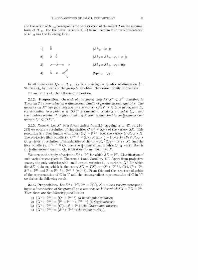
2. HV –VARIETIES OF SMALL CODIMENSION 61
and the action of H−M corresponds to the restriction of the weight Λ on the maximaltorus of H−M. For the Severi varieties 1)–4) from Theorem 2.9 this representationof H−M has the following form:
1)2 (SL2, 2ϕ1);
2)1 1 (SL2 × SL2, ϕ1 ⊕ ϕ1);
3) —1— (SL4 × SL2, ϕ2 ⊕ 0);
4)1——
(Spin10, ϕ1) .
In all these cases QΛ = H−M · xΛ is a nonsingular quadric of dimension 12n.
Shifting QΛ by means of the group G we obtain the desired family of quadrics.
2.5 and 2.11 yield the following proposition.
2.12. Proposition. On each of the Severi varieties Xn ⊂ PN described inTheorem 2.9 there exists an n-dimensional family of 1
2n-dimensional quadrics. Thequadrics on Xn are parametrized by the variety (SX)∗ ' X (the hyperplane Lα
corresponding to a point α ∈ (SX)∗ is tangent to X along a quadric Qα), andthe quadrics passing through a point x ∈ X are parametrized by an n
2 -dimensionalquadric Qx ⊂ (SX)∗.
2.13. Remark. Let Xn be a Severi variety from 2.9. Arguing as in [47, pp. 234–235] we obtain a resolution of singularities G ×P−M 〈QΛ〉 of the variety SX. Thisresolution is a fiber bundle with fiber 〈QΛ〉 = Pn
2 +1 over the variety G/P−M ' X.The projective fiber bundle PΛ ×PΛ∩P−M 〈QΛ〉 of rank n
2 + 1 over PΛ/PΛ ∩ P−M 'Q−M yields a resolution of singularities of the cone PΛ · 〈QΛ〉 = S(xΛ, X), and thefiber bundle PΛ ×PΛ∩P−M QΛ over the n
2 -dimensional quadric Q−M whose fiber isan n
2 -dimensional quadric QΛ is birationally mapped onto X.
We turn to the study of varieties Xn ⊂ PN for which SX = PN . Classification ofsuch varieties was given in Theorem 1.4 and Corollary 1.7. Apart from projectivespaces, the only varieties with small secant varieties (i. e. varieties Xn for whichdim SX ≤ 2n or, which is the same, SX = TX) are Qn ⊂ Pn+1, G(4, 1)6 ⊂ P9,S10 ⊂ P15 and P1 × Pn−1 ⊂ P2n−1 (n ≥ 3). From this and the structure of orbitsof the representation of G in V and the contragredient representation of G in V ∗
we derive the following result.
2.14. Proposition. Let Xn ⊂ PN , PN = P(V ), N > n be a variety correspond-ing to a linear action of the group G on a vector space V for which SX = TX = PN .Then there are the following possibilities:
1) Xn ⊂ PN = Qn ⊂ Pn+1 (a nonsingular quadric);2) Xn ⊂ PN = P1 × Pn−1 ⊂ P2n−1 (a Segre variety);3) Xn ⊂ PN = G(4, 1)6 ⊂ P9 (the Grassmann variety);4) Xn ⊂ PN = S10 ⊂ P15 (the spinor variety).
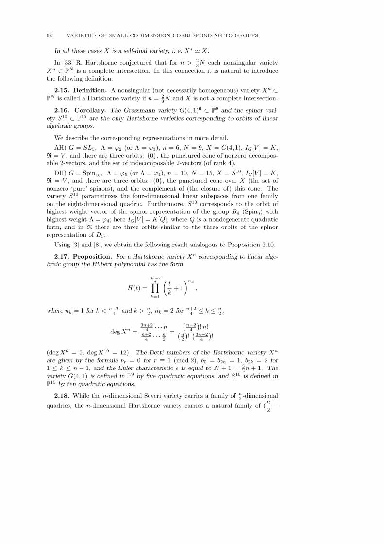
62 VARIETIES OF SMALL CODIMENSION CORRESPONDING TO GROUPS
In all these cases X is a self-dual variety, i. e. X∗ ' X.
In [33] R. Hartshorne conjectured that for n > 23N each nonsingular variety
Xn ⊂ PN is a complete intersection. In this connection it is natural to introducethe following definition.
2.15. Definition. A nonsingular (not necessarily homogeneous) variety Xn ⊂PN is called a Hartshorne variety if n = 2
3N and X is not a complete intersection.
2.16. Corollary. The Grassmann variety G(4, 1)6 ⊂ P9 and the spinor vari-ety S10 ⊂ P15 are the only Hartshorne varieties corresponding to orbits of linearalgebraic groups.
We describe the corresponding representations in more detail.
AH) G = SL5, Λ = ϕ2 (or Λ = ϕ3), n = 6, N = 9, X = G(4, 1), IG[V ] = K,N = V , and there are three orbits: 0, the punctured cone of nonzero decompos-able 2-vectors, and the set of indecomposable 2-vectors (of rank 4).
DH) G = Spin10, Λ = ϕ5 (or Λ = ϕ4), n = 10, N = 15, X = S10, IG[V ] = K,N = V , and there are three orbits: 0, the punctured cone over X (the set ofnonzero ‘pure’ spinors), and the complement of (the closure of) this cone. Thevariety S10 parametrizes the four-dimensional linear subspaces from one familyon the eight-dimensional quadric. Furthermore, S10 corresponds to the orbit ofhighest weight vector of the spinor representation of the group B4 (Spin9) withhighest weight Λ = ϕ4; here IG[V ] = K[Q], where Q is a nondegenerate quadraticform, and in N there are three orbits similar to the three orbits of the spinorrepresentation of D5.
Using [3] and [8], we obtain the following result analogous to Proposition 2.10.
2.17. Proposition. For a Hartshorne variety Xn corresponding to linear alge-braic group the Hilbert polynomial has the form
H(t) =
3n−24∏
k=1
(t
k+ 1
)nk
,
where nk = 1 for k < n+24 and k > n
2 , nk = 2 for n+24 ≤ k ≤ n
2 ,
deg Xn =3n+2
4 · · ·nn+2
4 · · · n2
=
(n−2
4
)!n!(
n2
)!(
3n−24
)!
(deg X6 = 5, deg X10 = 12). The Betti numbers of the Hartshorne variety Xn
are given by the formula br = 0 for r ≡ 1 (mod 2), b0 = b2n = 1, b2k = 2 for1 ≤ k ≤ n − 1, and the Euler characteristic e is equal to N + 1 = 3
2n + 1. The
variety G(4, 1) is defined in P9 by five quadratic equations, and S10 is defined inP15 by ten quadratic equations.
2.18. While the n-dimensional Severi variety carries a family of n2 -dimensional
quadrics, the n-dimensional Hartshorne variety carries a natural family of (n
2−
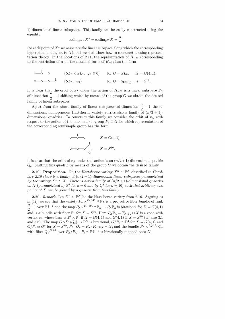
2. HV –VARIETIES OF SMALL CODIMENSION 63
1)-dimensional linear subspaces. This family can be easily constructed using theequality
codimPN∗ X∗ = codimPN X =n
2
(to each point of X∗ we associate the linear subspace along which the correspondinghyperplane is tangent to X), but we shall show how to construct it using represen-tation theory. In the notations of 2.11, the representation of H−M correspondingto the restriction of Λ on the maximal torus of H−M has the form
—1 (SL3 × SL2, ϕ2 ⊕ 0) for G = SL6, X = G(4, 1);
———1 (SL5, ϕ4) for G = Spin10, X = S10.
It is clear that the orbit of xΛ under the action of H−M is a linear subspace PΛ
of dimensionn
2− 1 shifting which by means of the group G we obtain the desired
family of linear subspaces.Apart from the above family of linear subspaces of dimension
n
2− 1 the n-
dimensional homogeneous Hartshorne variety carries also a family of (n/2 + 1)-dimensional quadrics. To construct this family we consider the orbit of xΛ withrespect to the action of the maximal subgroup Pe ⊂ G for which representation ofthe corresponding semisimple group has the form
—1—, X = G(4, 1);
——1
, X = S10.
It is clear that the orbit of xΛ under this action is an (n/2+1)-dimensional quadricQe. Shifting this quadric by means of the group G we obtain the desired family.
2.19. Proposition. On the Hartshorne variety Xn ⊂ PN described in Corol-lary 2.16 there is a family of (n/2 − 1)-dimensional linear subspaces parametrizedby the variety X∗ ' X. There is also a family of (n/2 + 1)-dimensional quadricson X (parametrized by P4 for n = 6 and by Q8 for n = 10) such that arbitrary twopoints of X can be joined by a quadric from this family.
2.20. Remark. Let Xn ⊂ PN be the Hartshorne variety from 2.16. Arguing asin [47], we see that the variety PΛ ×PΛ∩P−M PΛ is a projective fiber bundle of rankn
2−1 over Pn
2−1 and the map PΛ×PΛ∩P−MPΛ → PΛPΛ is birational for X = G(4, 1)
and is a bundle with fiber P1 for X = S10. Here PΛPΛ = TX,xΛ ∩X is a cone withvertex xΛ whose base is P1 × P2 if X = G(4, 1) and G(4, 1) if X = S10 (cf. also 3.1and 3.6). The map G×Pe 〈Qe〉 → PN is birational, G/Pe ' P4 for X = G(4, 1) andG/Pe ' Q8 for X = S10, PΛ ·Qe = PΛ ·Pe ·xΛ = X, and the bundle PΛ×PΛ∩Pe Qe
with fiber Qn/2+1e over PΛ/PΛ ∩ Pe ' Pn
2−1 is birationally mapped onto X.
64 VARIETIES OF SMALL CODIMENSION CORRESPONDING TO GROUPS
3. HV -varieties as birational images of projective spaces
As we already mentioned (cf. 1.1 and 1.3), from a general theorem of Rosenlicht[72] it follows that HV -varieties are rational. However for HV -varieties one cangive an explicit geometric construction of birational isomorphism with projectivespace.
3.1. Let Xn = GxΛ ⊂ PN be an HV -variety, where PN = P(V ), G is asemisimple group, G → AutV is an irreducible representation, and xΛ ∈ PN isthe point corresponding to highest weight vector vΛ ∈ V (here Λ is the highestweight). We denote by PΛ the stabilizer of the point xΛ (so that X ' G/PΛ),and let HΛ be the semisimple group corresponding to the parabolic subgroup PΛ.The representation of HΛ in V obtained by restricting the representation of G isreducible: it is clear that
HΛ · (KvΛ), HΛ · (gvΛ) = gvΛ,
where gvΛ is the tangent space to GvΛ at the point vΛ. Thus the HΛ-module Vcan be represented in the form
V = KvΛ ⊕ tV ⊕ nV, (3.1.1)
where KvΛ⊕ tV = gvΛ is the tangent and nV is the ‘normal’ subspace to GvΛ ⊂ Vat the point vΛ ∈ GvΛ.
It is clear that the subset GvΛ∩ (tV ⊕ nV ) is stable with respect to the action ofHΛ, and the stabilizer of an arbitrary point of GvΛ ∩ (tV ⊕ n) contains a maximalunipotent subgroup of HΛ. The corresponding projective variety H = X ∩ P(tV ⊕nV ) is the singular hyperplane section of X corresponding to the hyperplane P(tV ⊕nV ) ⊂ P(V ) which is tangent to X along the subvariety
Y = Sing H = X ∩ P(nV ). (3.1.2)
3.2. Next we consider the rational projection
πX = π∣∣X
: Xn 99K Pn, Pn = P(KvΛ ⊕ tV )
with center in the (N − n− 1)-dimensional linear subspace P(nV ) ⊂ PN . Let
Pn−1 = P(tV ) ⊂ Pn = P(KvΛ ⊕ tV ),
and let A ⊂ Pn−1 ⊂ Pn be the projective variety corresponding to GvΛ ∩ tV . Weobserve that, since X is defined in PN by quadratic equations (cf. [57]), Tn
X,xΛ∩X is
a cone with vertex xΛ. It is clear that A ⊂ Pn−1 is the base of this cone. Under theprojection π, the hyperplanes passing through P(nV ) are mapped onto hyperplanesin Pn. Furthermore,
π(P(tV ⊕ nV )
)= P(tV ) = Pn−1 ⊂ Pn,
andπ(H) = A ⊂ Pn−1.
The projection GvΛ → KvΛ ⊕ tV is a map of HΛ-spaces, and its fibers over pointslying in the same orbit are isomorphic to each other. It is not hard to see that allramification points of π lie in H , so that π
∣∣X\H is an isomorphism, π is a birational
isomorphism, and the variety X is rational.
3. HV –VARIETIES AS BIRATIONAL IMAGES OF PROJECTIVE SPACES 65
Summing up the discussion in 3.1 and 3.2, we obtain the following result.
3.3. Theorem. Let Xn ⊂ PN be a projective HV -variety. Then there exist alinear subspace M ⊂ PN , dim M = N − n− 1 and a hyperplane L ⊃ M such thatthe projection π : X 99K Pn with center in M is a birational isomorphism. Moreprecisely, if H = L∩X, then π
∣∣X\H is an isomorphism and π(H) ⊂ π(L) = A ⊂
Pn−1 = π(L) ⊂ Pn.3.4. For applications in Chapters IV and VI we need to know the structure
of representation R of the group HΛ in V for some specific representations of thegroup G. We proceed with listing the results of our computations (in what follows0 denotes the trivial representation, R(ψ) is the irreducible representation corre-sponding to weight ψ; in the case when HΛ is a simple group we denote by ϕi thei-th fundamental weight in the notations of Bourbaki [9]; if the group HΛ is notsimple, then HΛ is a product of two simple groups, ϕi denotes the i-th fundamentalweight of one of them, and ϕ′i the i-th fundamental weight of the other one; thefirst summand in the formulae below corresponds to the line KvΛ, the second tothe subspace tV and the third to the subspace nV ).
1) G = SLn+1, Λ = 2ϕ1, X = v2(Pn), HΛ = SLn, R = 0⊕R(ϕ1)⊕R(2ϕ1);2) G = SLa+1 × SLb+1, a, b ≥ 1, Λ = ϕ1 + ϕ′1, X = Pa × Pb, HΛ =
SLa × SLb, R = 0⊕ [R(ϕ1) + R(ϕ′1)]⊕R(ϕ1 + ϕ′1);3) G = SLm+1, m ≥ 3, Λ = ϕ2, X = G(m, 1), HΛ = SL2 × SLm−1, R =
0⊕R(ϕ1 + ϕ′1)⊕R(ϕ′2);4) G = E6, Λ = ϕ1, X = E16, HΛ = Spin10, R = 0⊕R(ϕ5)⊕R(ϕ1);5) G = Spin10, Λ = ϕ5, X = S10, HΛ = SL5, R = 0⊕R(ϕ3)⊕R(ϕ1).
3.5. If the representation of HΛ in nV is irreducible, then its lowest weight vectorcoincides with vM, where vM is the lowest weight vector of the representation of Gin V corresponding to the lowest weight M. Hence the variety Y corresponding tothe orbit of highest weight vector of the representation of HΛ in nV can be alsodefined by the following formulae:
Y = P−ΛxM = w0P−Mw0xM = w0P−MxΛ,
where P−Λ is the stationary subgroup of the lowest weight vector of the contragre-dient representation of G in V ∗. This allows to compute Y in cases 1)–5) from 3.4:
1) Y = v2(Pn−1), P(nV ) = 〈Y 〉 = Pn(n−1)
2 −1;2) Y = Pa−1 × Pb−1, P(nV ) = 〈Y 〉 = Pab−1;
3) Y = G(m− 2, 1), P(nV ) = 〈Y 〉 = Pm(m−3)
2 ;4) Y = Q8, P(nV ) = 〈Y 〉 = P9;5) Y = P−MPΛ = P4.
3.6. From 1.3 it follows that the representation of HΛ in tV is irreducible, andit is clear that A is an HΛ-variety. Using the explicit form of representation of HΛ
in tV computed in 3.4 it is easy to describe A in cases 1)–5):
66 VARIETIES OF SMALL CODIMENSION CORRESPONDING TO GROUPS
1) A = ∅;
2) A = Pa−1∐Pb−1;
3) A = P1 × Pm−2;
4) A = S10;
5) A = G(4, 1).
In case 1) π is an isomorphism, and in cases 2)–5) π∣∣X\H is an isomorphism and
π∣∣H
is a rational bundle with fiber:
2) Pb over Pa−1, Pa over Pb−1;
3) Pm−2;
4) P5;
5) P3.
3.7. Using tables in the end of [94] it is easy to verify that in cases 1)–5) from3.4 we have the following formulae (S2 denotes the second symmetric power):
1) S2(0⊕R(ϕ1)
) ' 0⊕R(ϕ1)⊕R(2ϕ1);
2) S2(0⊕ [R(ϕ1)⊕R(ϕ′1)]
) ' 0⊕ [R(ϕ1)⊕R(ϕ′1)]⊕R(ϕ1 + ϕ′1)⊕ [R(2ϕ1)⊕R(2ϕ′1)];
3) S2(0⊕R(ϕ1 + ϕ′1)
) ' 0⊕R(ϕ1 + ϕ′1)⊕R(ϕ′2)⊕R(2ϕ1 + ϕ′1);
4) S2(0⊕R(ϕ5)
) ' 0⊕R(ϕ5)⊕R(ϕ1)⊕R(2ϕ5);
5) S2(0⊕R(ϕ3)
) ' 0⊕R(ϕ3)⊕R(ϕ1)⊕R(2ϕ3).
It is easy to see that in these formulae the first term corresponds to the summandKvΛ, the second term to the summand tV , and the third one to the summand nVin decomposition (3.1.1). From this and 3.2 it follows that the linear system ofquadrics in TX,xΛ containing the subvariety A ⊂ Pn−1 ⊂ TX,xΛ defines a rationalmap
σ : Pn 99K P(KvΛ ⊕ tV ⊕ nV ),
which is inverse to π. From formulae 1)–5) it also follows that all the above varietiesare rational projections of the Veronese varieties v2(Pn), viz.
1) X = v2(Pn);
2) the Segre variety Pa × Pb is obtained from v2(Pa+b) by projecting it from〈v2(Pa−1), v2(Pb−1)〉, Pa−1 ∩ Pb−1 = ∅;
3) the Grassmann variety G(m, 1) is obtained from v2(P2m−2) by projectingit from 〈v2(P1)× v2(Pm−2)〉;
4) E16 is obtained from v2(P16) by projecting it from 〈v2(S10)〉 = P125;
5) S10 is obtained from v2(P10) by projecting it from 〈v2(G(4, 1)〉 = P49.
Summing up the discussion in 3.4–3.7, we obtain the following result.
3. HV –VARIETIES AS BIRATIONAL IMAGES OF PROJECTIVE SPACES 67
3.8. Theorem. 1) Let X = v2(Pn) ⊂ Pn(n+3)
2 . The projection π : X → Pn
with center in 〈v2(Pn−1)〉 is an isomorphism inverse to the Veronese mapσ = v2 : Pn → X.
2) Let X = Pa × Pb ⊂ Pab+a+b. The projection π : X 99K Pa+b with center in〈Pa−1 × Pb−1〉 is a birational isomorphism; moreover, if H = Pa × Pb−1 ∩Pa−1×Pb, then π
∣∣X\H is an isomorphism. The inverse map σ : Pa+b 99K X
is defined by the linear system of quadrics passing through Pa−1∐Pb−1 ⊂
Pa+b−1 ⊂ Pa+b. The variety X is obtained from the Veronese varietyv2(Pa+b) by projecting it from 〈v2(Pa−1), v2(Pb−1)〉.
3) Let X = G(m, 1) ⊂ Pm2+m−2
2 . The projection π : X 99K P2(m−1) withcenter in 〈G(m − 2, 1)〉 is a birational isomorphism; moreover, if H is theSchubert divisor corresponding to a subspace Pm−2 ⊂ Pm, then π
∣∣X\H is an
isomorphism. The inverse map σ : P2(m−1) 99K X is defined by the linearsystem of quadrics containing the Segre variety P1 × Pm−2 ⊂ P2m−3 ⊂P2(m−1). The variety X is obtained from the Veronese variety v2(P2(m−1))by projecting it from 〈v2(P1)× v2(Pm−2)〉.
4) Let X = E16 ⊂ P26. The projection π : X 99K P16 with center in 〈Q8〉 = P9,where Q8 ⊂ P16 is a nonsingular quadric, is a birational isomorphism;moreover, if H is the hyperplane section of X such that Sing H = Q8, thenπ∣∣X\H is an isomorphism. The inverse map σ : P16 99K X is defined by the
linear system of quadrics containing the spinor variety S10 ⊂ P15 ⊂ P16
parametrizing four-dimensional linear subspaces from one family on theeight-dimensional quadric. The variety X is obtained from the Veronesevariety v2(P16) ⊂ P152 by projecting it from 〈v2(S10)〉 = P125.
5) Let X = S10 ⊂ P15. The projection π : X 99K P10 with center in a lin-ear subspace P4 ⊂ X is a birational isomorphism; moreover, if H is asingular hyperplane section, then π
∣∣X\H is an isomorphism. The inverse
map σ : P10 99K X is defined by the linear system of quadrics containing theGrassmann variety G(4, 1) ⊂ P9 ⊂ P10. The variety X is obtained from theVeronese variety v2(P10) ⊂ P65 by projecting it from 〈v2
(G(4, 1)
)〉 = P49.
3.9. Remark. In Theorem 3.8 we described projections of those HV -varietieswhich will be discussed in Chapters IV and VI and analyzed the structure of mapsπ∣∣H
and σ = π−1. Some other HV -varieties for which H may contain more than twoorbits of the group HΛ and σ has a more complex structure also present geometricinterest. A direct application of Theorem 3.3 shows that for all d > 1 projection ofthe Veronese variety vd(Pn) with center in a subspace 〈vd(Pn−1)〉 is an isomorphisminverse to vd; the Grassmann variety G(m, k) can be birationally projected ontoP(k+1)(m−k), and the fundamental subset A = π(H) of the map σ coincides withthe Segre variety
Pk × Pm−k−1 ⊂ P(k+1)(m−k)−1 ⊂ P(k+1)(m−k);
the spinor variety Sk parametrizing the k-dimensional linear subspaces from onefamily on a nonsingular 2k-dimensional quadric Q2k ⊂ P2k+1 (Sk corresponds to
68 VARIETIES OF SMALL CODIMENSION CORRESPONDING TO GROUPS
the orbit of highest weight vector of the spinor representation of the group Dk+1 =Spin2k+2) can be birationally projected onto P
k(k+1)2 , and the fundamental subset
A = π(H) of the map σ coincides with the Grassmann variety G(k, 1) ⊂ P k(k+1)2 −1 ⊂
Pk(k+1)
2 , etc. Nonsingular hyperplane sections of Severi varieties (examples A0), A2),C), and F) from § 2) can also be interpreted in this way (for such a variety A is ahyperplane section of the variety A for the corresponding Severi variety).
3.10. Remark. In the case of Segre variety P2×P2 and Grassmannians existenceof a birational projection π : X 99K Pn was proved by different methods in theclassical papers [79] and [81].
CHAPTER IV
SEVERI VARIETIES
Typeset by AMS-TEX
69
70 IV. SEVERI VARIETIES
1. Reduction to nonsingular case
1.1. The goal of this chapter is to give classification of extremal varieties withsmall secant varieties, i.e. varieties for which the inequality in Theorem 2.8 of Chap-ter II turns into equality. In other words, we classify nondegenerate varieties
Xn ⊂ PN , n =2N + b
3− 1, b = dim (Sing X) (1.1.1)
which can be J-isomorphically projected to PN−1. By Proposition 1.5 of Chapter II,the last condition holds if and only if SX 6= PN (in view of Remark 2.10 in Chap-ter II, for n > 1 this condition can be replaced by the condition T ′X 6= PN which,according to Proposition 1.5 of Chapter II, ensures the existence of a J-unramifiedprojection of X to PN−1. From Theorem 2.8 of Chapter II it follows that underthese assumptions
dim SX = N − 1 =3n− b + 1
2. (1.1.2)
Moreover, from Theorem 2.3 of Chapter V and Theorems 1.4 and 4.7 of the presentchapter it follows that if
X ′ ⊂ PN ′, SX ′ 6= PN ′
, dim X ′ = n,
dim (Sing X ′) = b, dim SX ′ =3n− b + 1
2
(1.1.3)
is a nondegenerate variety, then N ′ = N = 3(n+1)−b2 (a priori one can only claim
that any variety X ′ satisfying (1.1.3) can be J-isomorphically projected onto avariety X satisfying (1.1.1)).
Throughout this chapter we consider varieties defined over an algebraically closedfield K, charK = 0. We recall the following definition (cf. Definition 2.3 in Chap-ter III).
1.2. Definition. A nondegenerate nonsingular variety Xn ⊂ PN , n = 23 (N−2)
is called Severi variety if X can be isomorphically projected to PN−1.
In view of Proposition 1.5 b), d) and Corollary 1.7 from Chapter II, a nonsingularnondegenerate variety Xn ⊂ PN , n = 2
3 (N − 2) is a Severi variety if any of thefollowing equivalent conditions holds:
a) SX 6= PN ;b) there exists an unramified projection of X to a projective space of smaller
dimension;c) TX 6= PN .
1.3. Remark. Severi varieties are named after Francesco Severi who gave theirclassification in the case n = 2 (cf. [82] and also [62; 15]). More historical details aregiven in Remark 4.11. We recall that in Chapter III (cf. Theorem 2.9) we gave fourexamples of Severi varieties in dimensions 2, 4, 8, and 16, viz. the Veronese surfacev2(P2) ⊂ P5, the Segre variety P2×P2 ⊂ P8, the Grassmann variety G(5, 1)8 ⊂ P14,and the variety E16 ⊂ P26 corresponding to the orbit of highest weight vector ofthe simplest nontrivial representation of the group E6. In Theorem 4.7 we showthat these are the only Severi varieties.
1. REDUCTION TO NONSINGULAR CASE 71
1.4. Theorem. Let Xn ⊂ PN , SX 6= PN be a nondegenerate variety satisfyingcondition (1.1.1) (so that X has maximal possible dimension for given N and b).Then X is a projective cone with vertex Pb = Sing X whose base is a Severi varietyXn−b−1
0 ⊂ PN−b−1. Conversely, let Xn00 ⊂ PN0 be a Severi variety, let b ≥ 0 be an
integer, and let Xn ⊂ PN , n = n0 + b + 1, N = N0 + b + 1 be the projective coneover X0 with vertex Pb. Then SX 6= PN , Sing X = Pb, and n = 2N+b
3 − 1.
Proof. We already observed that SX is a hypersurface (cf. (1.1.2)). Let z be ageneral point of SX, and let Yz = p1(ϕ−1(z)) (cf. Chapter II, (2.8.1)). Since forour variety X the inequality in Theorem 2.8 of Chapter II turns into equality, fromthe proof of this theorem it immediately follows that dim (Yz ∩ Sing X) = b, i.e.there exists an irreducible component Ξ of the variety Sing X such that
dimΞ = b, Ξ ⊂⋂
z∈SX
Yz (1.4.1)
(cf. Remark 2.13 in Chapter II). From Proposition 1.9 of Chapter II it follows that
Yz ⊂ TSX,z. (1.4.2)
Combining (1.4.1) and (1.4.2), we see that
Ξ ⊂⋂
z∈SX
TSX,z. (1.4.3)
Since charK = 0, from (1.4.1) and (1.4.3) it follows that SX is a cone with vertex
Ξ = Pb ⊂ X ⊂ SX (1.4.4)
(to verify this without computations it suffices to refer to C. Segre’s reflexivitytheorem (cf. e.g. [49; 50])).
Let x ∈ Ξ, let y, y ′ be a general pair of points of X, and let z be a general pointof the chord 〈y, y ′〉. Since SX is a cone with vertex x, TSX,z ′ = TSX,z for all pointsz ′ ∈ 〈x, z〉r x. Therefore from Proposition 1.9 a) of Chapter II it follows that thehyperplane TSX,z is tangent to X at all points of Yz ∩ Sm X, where
Yz = p1 (ϕ−1(〈x, z〉r x)) =⋃
z ′∈〈x,z〉rx
Yz ′ .
Applying the arguments used in the proof of Theorem 2.8 of Chapter II to thesubvariety Yz (or applying Theorem 1.7 of Chapter I to the subvariety π(Yz) ⊂π(X) ⊂ Pn−1 and the hyperplane π(TSX,z) ⊂ PN−1, where π is the projection withcenter in a general point of TSX,z \ SX), we see that
dimYz = dim Yz =n + b + 1
2= 2n−N + 2.
Thus Yz consists of components of Yz, and we may assume that
Yz ′ ⊃ Yz (1.4.5)
72 IV. SEVERI VARIETIES
for z ′ ∈ 〈x, z〉. From (1.4.5) it follows that
C = p2
((p1 × ϕ)−1(y ′ × 〈x, z〉)) ⊂ X ∩Π
is a one-dimensional subvariety of the plane Π = 〈x, y ′, z〉. Without loss of generalitywe may assume that
〈x, z〉 ∩ C1 = 〈x, z〉 ∩X = x,
where C1 is a one-dimensional component of C passing through y. In fact, otherwiseSX = S(x,X) and therefore
dim Yz = 2n + 1− dim SX = 2n + 1− dim S(x,X) = n,
so that Yz = X and from (1.4.2) it follows that X ⊂ TSX,z contrary to the as-sumption that X is nondegenerate. From (1.4.6) it follows that a general line in Πpassing through x intersects C1 only at x, and therefore C1 = 〈x, y〉 (cf. e.g. [64,5.11]).
Thus for a general and therefore for each point y ∈ X we have 〈x, y〉 ⊂ X, i.e.X is a cone with vertex x. Since x is an arbitrary point of Ξ, from this it followsthat X is a cone with vertex Ξ = Pb, and since X is irreducible, b < n− 1.
Let MN0 ⊂ PN be a general linear subspace, M ∩ Sing X = ∅, N0 = N − b− 1,X0 = X ∩ M , n0 = dim X0 = n − b − 1 > 0. By Bertini’s theorem (cf. [28,Vol. I, Chapter I, § 1; 34, Chapter II, 8.18]), X0 is irreducible and nonsingular.Furthermore,
SX0 ⊂ SX ∩M 6= M
and
n0 = n− b− 1 =(
2N + b
3− 1
)− b− 1 =
2(N − b− 1)− 43
=23(N0 − 2),
i.e. X0 is a Severi variety.The converse is an immediate consequence of the fact that, as it is easy to see,
SX is the cone over SX0 with vertex Pb = Sing X, and since n0 = 23 (N0 − 2),
n = n0 + b + 1 =2(N0 + b + 1) + b− 3
3=
2N + b
3− 1.
¤
2. QUADRICS ON SEVERI VARIETIES 73
2. Quadrics on Severi varieties
2.1. Proposition. Let Xn ⊂ PN , n = 23 (N − 2) be a Severi variety, and let
z be a general point of SX. Set L = TSX,z, P L = u ∈ SX∣∣ TSX,u = L. Then
X∩P L = Yz = p1(ϕ−1(z)) is a nonsingular n2 -dimensional quadric in the projective
space P L = Pn2 +1.
Proof. According to C. Segre’s reflexivity theorem (cf. [49; 50]), P L is a linearsubspace of PN .
LetXL = x ∈ X
∣∣ TX,x ⊂ L.Then XL is a closed subvariety of X, T (XL, X) ⊂ L, and since X is nondegenerate,S(XL, X) 6⊂ L. Hence Theorem 1.4 of Chapter I shows that
dim SX =3n
2+ 1 ≥ dim S(XL, X) = dim XL + n + 1,
so thatdim XL ≥ n
2. (2.1.1)
On the other hand, for a general point u ∈ P L from Proposition 1.9 of Chapter IIit follows that
T (Yu, X) ⊂ TSX,udef= L, Yu = p1(ϕ−1(u)),
i.e.Yu ⊂ XL. (2.1.2)
Since X is a Severi variety, we have
dim Yz = dim Yu = 2n + 1− dim SX = 2n + 1−(
3n
2+ 1
)=
n
2. (2.1.3)
Combining (2.1.1), (2.1.2), and (2.1.3), we see that for a general point u ∈ P L wehave Yu = Yz. Therefore
SYz = P L (2.1.4)
and by (2.1.3)
2 dim Yz + 1− dim P L = dim Yz, dim P L = dim Yz + 1 =n
2+ 1,
so that P L = Pn2 +1 and Yz is a hypersurface in Pn
2 +1. Hence for a general pointu ∈ P L there is an inclusion Yu ⊃ X ∩ P L, and therefore
X ∩ P L = Yz. (2.1.5)
From (2.1.4) it follows that deg Yz ≥ 2. From the trisecant lemma (cf. [39, 2.5]and also [34, Chapter IV, § 3] and [64, § 7B]) it follows that for a general pair ofpoints x, y ∈ X
〈x, y〉 ∩X = x, y. (2.1.6)
74 IV. SEVERI VARIETIES
Since z is a general point of SX, from (2.1.6) it follows that deg Yz = 2.It remains to verify that the quadric Yz is nonsingular. Suppose that this is
not so. Then Yz is a quadratic cone with vertex at a point y ∈ Yz. ThereforeSX = S(Yz, X) is a cone with vertex y, and for a general point u ∈ SX we havey ∈ PM , M = TSX,u. In view of (2.1.5), from this it follows that
y ∈⋂
u∈SX
Yu. (2.1.7)
From (2.1.2) and (2.1.7) it follows that TX,y ⊂⋂u
TSX,u, i.e. SX is a cone with
vertex TX,y andTX,y ⊂
⋂
M
PM
which is impossible since
dim PM =n
2+ 1 ≤ n = dim TX,y.
This contradiction shows that Yz is a nonsingular quadric. ¤2.2. Lemma. Let Xn ⊂ PN , n = 2
3 (N − 2) be a Severi variety, and let zbe a general point of SX. Then, in the notations of Section 1 of Chapter I, themorphism ϕz = ϕYz : SYz,X → S(Yz, X) = SX, Yz = p1(ϕ−1(z)) is birational.
Proof. From Proposition 1.9 a) of Chapter II it follows that
T (Yz, X) ⊂ TN−1SX,z ,
and since〈S(Yz, X)〉 = 〈X〉 = PN ,
Theorem 1.4 of Chapter I shows that
dim S(Yz, X) = dim SYz,X = dim SX = N − 1 =3n
2+ 1.
Hence S(Yz, X) = SX and the morphism ϕz is generically finite, i.e. for a generalpoint u ∈ SX we have card (Yz ∩ Yu) < ∞. To prove Lemma 2.2 it suffices toverify that for a general point u ∈ SX the quadrics Yz and Yu (cf. Proposition 2.1)transversely intersect at a unique point (Yz ∩ Yu 6= ∅ since u ∈ S(Yz, X) = SX).
Let Pz (resp. Pu) be the (n2 + 1)-dimensional linear subspace spanned by the
quadric Yz (resp. Yu). Suppose that Yz ∩ Yu 3 x, y, and let l = 〈x, y〉 (in the casewhen y = x, i.e. Yz and Yu are tangent at x, l is their common tangent line). Then
l ⊂ Pz ∩ Pu ⊂ Sing (SX)
since by Proposition 2.1 the tangent space to SX at an arbitrary point of Pz ∩ Pu
contains both TSX,z and TSX,u 6= TSX,z. Varying u ∈ SX, we see that a generalpoint y ∈ Yz lies on a line ly ⊂ Pz ∩ (Sing X \X), from which it follows thatz ∈ Pz ⊂ Sing SX contrary to the choice of z. This contradiction completes theproof of Lemma 2.2. ¤
2. QUADRICS ON SEVERI VARIETIES 75
2.3. Lemma. Let Xn ⊂ PN , n = 23 (N − 2) be a Severi variety. Then the
quasiprojective variety SX \X has nonsingular normalization.
Proof. Let v ∈ Sing (SX \X), and let Y ′v be an irreducible component of Yv =
p1(ϕ−1(v)). Then eitherS(Y ′
v , X) 6= SX (2.3.1)
and for a general point z ∈ SX
Yz ∩ Y ′v = ∅ (2.3.2)
orS(Y ′
v , X) = SX. (2.3.3)
We claim that in the case (2.3.3)
dim Y ′v =
n
2. (2.3.4)
Suppose that this is not so and
dim Y ′v > 2n + 1− dim SX =
n
2. (2.3.5)
In view of (2.3.3) and Theorem 1.4 of Chapter I, from (2.3.5) it follows that
T (Y ′v , X) = SX. (2.3.6)
Remark 1.10 in Chapter II shows that if v ∈ 〈y, x〉, y ∈ Y ′v , x ∈ X, x 6= y, then
T ′v,S(x,X) ⊃ TX,y, where T ′v,S(x,X) is the tangent cone to S(x,X) at the point v (weuse the notations of § 1 of Chapter I). Therefore
T ′v,SX ⊃ T ′v,S(x,X) ⊃ TX,y.
On the other hand, if v ∈ TX,y, then it is clear that T ′v,SX ⊃ TX,y. Thus
T (Y ′v , X) ⊂ T ′v,SX . (2.3.7)
Combining (2.3.6) and (2.3.7) we see that SX ⊂ T ′v,SX , i.e. SX is a cone withvertex v. Hence, in the notations of Lemma 2.2,
v ∈⋂
z∈X
Pz. (2.3.8)
But in the proof of Lemma 2.2 we verified that for a general pair of points z, u ∈ SXthe variety Pz∩Pu = Yz∩Yu reduces to a unique point lying in X, which contradicts(2.3.8). This contradiction proves (2.3.4).
From (2.3.2) and (2.3.4) it follows that for a general point z ∈ SX we havecard (Yz ∩ Yu) < ∞, i.e. in the notations of Lemma 2.2 ϕ−1
z (v) is a finite set. HenceLemma 2.2 and Proposition 2.1 show that in a neighborhood of v the normalizationof SX = S(Yz, X) is isomorphic to SYz,X and therefore is nonsingular. Lemma 2.3is proved. ¤
76 IV. SEVERI VARIETIES
2.4. Theorem. Let Xn ⊂ PN , n = 23 (N − 2) be a Severi variety. Then
a) SX is a normal hypersurface and Sing SX = X;b) Each point z ∈ SX \X is general in the sense of Proposition 2.1, i.e. Yz is
a nonsingular quadric in the projective space Pz = Pn2 +1;
c) ϕ∣∣ϕ−1(SX\X)
is a smooth morphism, and the tangent spaces at arbitrary
points x, y ∈ X such that the line 〈x, y〉 does not lie in X span a hyperplane,i.e. dim 〈TX,x, TX,y〉 = N − 1 = 3n
2 + 1;d) An arbitrary secant of the variety X either lies on X or intersects X at
exactly two points (which may coincide with each other);e) SX is a cubic and multx SX = 2 for each point x ∈ X = Sing SX (here
multx SX denotes the multiplicity of x on SX);f) For an arbitrary point z ∈ SX \X the projection with center in Pz defines
a birational map πz : X 99K Pn which is an isomorphism outside X∩TSX,z.
Proof. a) Let
ϕ = νϕ, ϕ : SX → SX, ν : SX → SX
be the Stein factorization of the morphism ϕ : SX → SX. From Proposition 2.1 itfollows that ν : SX → SX is the normalization morphism. Lemma 2.3 shows that
Sing SX ⊂ ν−1(X). (2.4.1)
Suppose that Sing SX 6= X, let v be a general point of Sing (SX \X), and letv ∈ ν−1(v). In view of (2.4.1) and the Serre normality criterion (cf. e.g. [30,Chapter IV2, (5.8.6)]),
dim(Sing (SX \X)
)= dim SX − 1 =
3n
2.
Hence dim ϕ−1(v) = n2 and ϕ∗([v]) ≡ [ϕ−1(z)], where z is a general point of SX,
brackets denote the cycle corresponding to subvariety, and ≡ denotes algebraicequivalence. Therefore
(p1)∗(ϕ∗([v])
)= (p1)∗
([ϕ−1(z)]
)= [Yz]. (2.4.2)
By Proposition 2.1 and Lemma 2.2, Yz is a nonsingular quadric and
(Y 2
z
)X
= 1. (2.4.3)
Hence all components of Yv = p1(ϕ−1(v)) are also n2 -dimensional quadrics. From
(2.4.2) and (2.4.3) it follows that for a general point v ∈ Sing X \X the fiber ϕ−1(v)is connected, i.e. the morphism ν is one-to-one. Since for x ∈ X the fiber ϕ−1(x)is connected and contains a reduced component (which is isomorphic to X), fromthis it follows that ν is an isomorphism, i.e. SX is a normal hypersurface. FromLemma 2.3 it follows that Sing SX ⊂ X. On the other hand, Lemma 1.8 a) fromChapter II shows that X ⊂ Sing SX. Thus X = Sing SX. Assertion a) is proved.
2. QUADRICS ON SEVERI VARIETIES 77
b) Let z ∈ SX \X be an arbitrary point. Then from a) and Proposition 1.9 a)in Chapter II it follows that
T (Yz, X) ⊂ TSX,z 6= PN .
Since S(Yz, X) ⊃ X,S(Yz, X) 6= T (Yz, X),
and from Theorem 1.4 of Chapter I it follows that
dim S(Yz, X) = dim Yz + n + 1, S(Yz, X) = SX, dim Yz =n
2. (2.4.4)
We already proved in a) that under these conditions Yz is a quadric. Moreover, inthe proof of Proposition 2.1 it is shown that from (2.4.4) it easily follows that thequadric Yz is nonsingular. Assertion b) is proved.
c) The first claim follows from b), and the second claim is a consequence of thefirst one and the proof of Proposition 1.9 b) in Chapter II.
d) immediately follows from b).e) Let x be an arbitrary point of X, and let Qx = p1
(ψ−1(x)
)(we use the
notations of § 1 of Chapter I). We observe that S(Qx, X) 6= SX. In fact, otherwisefrom Proposition 1.9 a) of Chapter II it would follow that x ∈ ⋂
z∈SX
TSX,z, i.e.
SX is a cone with vertex x, which is impossible in view of b) and the proof ofProposition 2.1.
Let z ∈ SX \ S(Qx, X), and let Pn2 +2
z,x = 〈Pz, x〉. Then
Pz,x ∩X = Yz ∪ x, (2.4.5)
and the intersection of subvarieties Pn2 +2
z,x and Xn at the point x of the projectivespace P 3n
2 +2 is transverse. In fact, if
x ′ ∈ Pz,x ∩X, x ′ /∈ Yz, u ∈ 〈x, x ′〉 ∩ Pz,
then in view of the choice of z
x /∈ T (Yz, X) (2.4.6)
and from d) it follows that u /∈ X, so that b) yields Yu = Yz which is impossible by(2.4.6) since it is clear that Yu 3 x.
Now let u ∈ Pz,x∩SX be an arbitrary point. As we already observed, Yu∩Yz 6=∅, and either
u ∈ TX,y ∩ Pz,x, y ∈ Yz (2.4.7)
oru ∈ 〈y, x ′〉, y ∈ Yz, x ′ ∈ X ∩ Pz,x. (2.4.8)
But(TX,y ∩ Pz,x) ⊂ (T (Yz, X) ∩ Pz,x) = P
n2 +1
z , (2.4.9)
78 IV. SEVERI VARIETIES
and from (2.4.5), (2.4.7), (2.4.8), and (2.4.9) it follows that
Pz,x ∩ SX = Pz ∪ SxYz. (2.4.10)
Assertion e) immediately follows from (2.4.10).f) immediately follows from the proof of assertion e).
¤2.5. Remark. From Theorem 2.4 b) it follows that
S(SX)∗ ⊂ X∗. (2.5.1)
Counting dimensions, we see that each hyperplane in PN which is tangent to X ata point x ∈ X lies in the pencil generated by two hyperplanes which are tangent toSX at some points of S(x,X) (cf. Proposition 3.1 for more details). Therefore
S((SX)∗
)= X∗. (2.5.2)
Applying Theorem 2.4 (and specifically assertion e) of this theorem), it is not hardto show that the variety X = Sing SX is an intersection of quadrics and the linearsystem of quadrics passing through X defines a birational map
κX : PN 99K PN , (2.5.3)
under which SX is transformed to X and vice versa (if F (x0 : · · · : xN ) = 0 isthe equation of the cubic hypersurface SX, then κX is defined by the formula
κX(x) =(
∂F
∂x0(x) : · · · : ∂F
∂xN(x)
)). Since by definition κX(SX) = X∗, from this
it follows thatX∗ ' SX, (SX)∗ ' X. (2.5.4)
3. DIMENSION OF SEVERI VARIETIES 79
3. Dimension of Severi varieties
3.1. Proposition. Let Xn ⊂ PN , N = 23 (N − 2) be a Severi variety, let
x ∈ X be an arbitrary point, and let Y x = (TSX,z)∗∣∣ z ∈ S(x,X) \X (here
(TSX,z)∗ ∈ PN∗ is the point corresponding to the hyperplane TSX,z). Then Y x is anonsingular quadric in the (n
2 + 1)-dimensional projective space (TX,x)∗ ⊂ PN∗.
Proof. It is clear that Y x is an irreducible variety. Since dim S(x,X) = n + 1and for z ∈ S(x,X) \X the hyperplane TSX,z is tangent to SX along the (n
2 + 1)-dimensional linear subspace
Pz = SYz ⊂ S(x,X),
we conclude thatdim Y x = (n + 1)− (
n
2+ 1) =
n
2.
From Theorem 2.4 it follows that Y x is a (closed) irreducible hypersurface in(TX,x)∗. Since the variety (SX)∗ ⊂ PN∗ is not a hypersurface (cf. e.g. (2.5.1)),from the trisecant lemma (cf. [39, 2.5] and also [34, Chapter IV, § 3] and [64, §7B])it follows that deg Y x = 2.
It remains to show that the quadric Y x is nonsingular. In fact, otherwise thequadric Y x would be a cone, so that there would exist a point z ∈ S(x,X)\X suchthat
dim (Yz ∩ Yu) > 0 ∀u ∈ S(x,X) \X,
which contradicts Theorem 2.4 f). ¤3.2. Proposition. Let Xn ⊂ PN , n = 2
3 (N − 2) be a Severi variety, and letz1, z2 ∈ SX \ X. Then either z1 ∈ Pz2 , z2 ∈ Pz1 and Yz1 = Yz2 , Pz1 = Pz2 orYz1 ∩ Yz2 is a linear subspace (we use the notations from the proof of Lemma 2.2).
Proof. As we have already observed,
S(Yzi , X) = SX, i = 1, 2,
and therefore Yz1 ∩Yz2 6= ∅. Suppose that Yz1 ∩Yz2 is not a linear subspace. Thenfrom Theorem 2.4 it follows that
S(Yz1 ∩ Yz2) = Pz1 ∩ Pz2 6⊂ X.
But for an arbitrary point z ∈ S(Yz1 ∩Yz2) \X from Theorem 2.4 b) it follows that
Yz1 = Yz = Yz2 .
¤Let Xn ⊂ PN , N = 2
3 (n − 2) be a Severi variety, let x be an arbitrary point ofX, and let
Y1 = Yz1 , Y2 = Yz2 , z1, z2 ∈ S(x,X) \X
be two quadrics for which (Y1 · Y2) = x (cf. Lemma 2.2). Put
Ci = Yi ∩ TX,x = Yi ∩ TYi,x, i = 1, 2.
Then Ci is an (n2−1)-dimensional cone with vertex x in the n
2 -dimensional projectivespace TYi,x whose base is a nonsingular (n
2 − 2)-dimensional quadric (i = 1, 2). Itis clear that for n > 2, S(C1, C2) 6⊂ X (here, as in § 1 of Chapter I, S(C1, C2) is thejoin of cones C1 and C2).
80 IV. SEVERI VARIETIES
3.3. Proposition. a) dim S(C1, C2) = n− 2;b) Let n > 2, z ∈ S(C1, C2) \X, Yz 6= Yi (i = 1, 2). Then Yz ∩ Yi is a linear
subspace of dimension[
n4
];
c) For n > 2 we have n ≡ 0 (mod 4);d) For n > 4 we have n ≡ 0 (mod 8).
Proof. a) Let Qi be the base of the cone Ci (i.e. Qi is the intersection of Ci witha general hyperplane in TYi,x, i = 1, 2). Then
S(C1, C2) = S(x, S(Q1, Q2))
and〈Q1〉 ∩ 〈Q2〉 = ∅.
Hencedim S(C1, C2) = dim S(Q1, Q2) + 1 = 2(
n
2− 2) + 2 = n− 2.
Assertion a) is proved.b), c). Let z be a general point of S(C1, C2) \X. By Proposition 3.2,
Yz ∩ Yi = Pαi , i = 1, 2.
Since C1 and C2 are cones with vertex x, αi > 0 (i = 1, 2) and
Pαi 3 x, i = 1, 2 Pα1 ∩ Pα2 = C1 ∩ C2 = Y1 ∩ Y2 = x, z ∈ S(Pα1 ,Pα2).
Furthermore, if z ′ ∈ S(C1, C2) \X, then Yz ′ = Yz if and only if
z ′ ∈ S(Pα1 ,Pα2) = Pα1+α2 \X. (3.3.1)
By a) and (3.3.1), varying z ∈ S(C1, C2) \X we obtain an((n − 2) − (α1 + α2)
)-
dimensional family of quadrics passing through x and intersecting Y1 and Y2 alonglinear subspaces of positive dimension.
We already know (cf. Proposition 3.1) that there is an n2 -dimensional family of
quadrics Yu passing through x and parametrized by a quadric Y x. Furthermore,the (n
2 − 1)-dimensional subfamily of quadrics Yu intersecting Y1 along a positive-dimensional linear subspace is parametrized by the subcone with vertex (TSX,z1)
∗
in Y x. From this it follows that the dimension of the family of quadrics Yu passingthrough x and intersecting Y1 and Y2 along positive-dimensional linear subspacesis equal to n
2 − 2 (the base Y12 of this family is the intersection of two (n2 − 1)-
dimensional subcones in Y x with vertices (TSX,z1)∗ and (TSX,z2)
∗, so that Y12 isan (n
2 − 2)-dimensional quadric). Thus (n− 2)− (α1 + α2) = n2 − 2, i.e.
α1 + α2 =n
2. (3.3.2)
On the other hand, it is well known (cf. e.g. [37, Chapter XIII, § 4; 28, Chapter VI,§ 1]) that the maximal dimension of linear subspace lying on a nonsingular n
2 -dimensional quadric Yi (i = 1, 2) is equal to
[n4
]. Hence
αi ≤[n
4
], i = 1, 2. (3.3.3)
3. DIMENSION OF SEVERI VARIETIES 81
Combining (3.3.2) and (3.3.3), we see that
α1 = α2 =[n
4
]=
n
4
which simultaneously proves b) and c) (under specialization of z the dimension ofYz ∩ Yi could only jump).
d) Let z ∈ S(C1, C2) \ X. From b), c), and Proposition 3.1 it follows that theset of quadrics Yu passing through x and intersecting Yz along a linear subspace ofdimension n
4 is parametrized by the cone with vertex (TSX,z)∗ in Y x whose base isa nonsingular (n
2 − 2)-dimensional quadric. For n > 4 this cone is irreducible, andtherefore all n
4 -dimensional linear subspaces of the form Yz ∩ Yu belong to one andthe same family of linear subspaces on Yz. It is well known (cf. [37, Chapter XIII,§ 4; 28, Chapter VI, § 1]) that the dimension of intersection of two n
4 -dimensionallinear subspaces from one family on Y x has the same parity as n
4 (we recall that onthe nonsingular even-dimensional quadric Y
n2
z there exist two irreducible familiesof n
4 -dimensional linear subspaces). On the other hand, in the notations used inthe proof of assertions b) and c)
Pα1 ∩ Pα2 = Y1 ∩ Y2 = x.
Hence for n > 40 ≡ n
4(mod 2).
This completes the proof of assertion d).¤
3.4. Remark. Assertions c) and d) of Proposition 3.3 were independently provedby Fujita and Roberts (cf. Propositions 5.2 and 5.4 in [25]) who used the techniquesof computations with Chern classes. Their approach was developed by Roberts(unpublished) and Tango [89] (cf. Remark 4.11 below).
3.5. Corollary. If in the conditions of Proposition 3.2 Yz1 6= Yz2 , then Yz1∩Yz2
is either a point or a linear subspace of dimension n4 .
In the proof of Proposition 3.3 we showed that varying z in S(C1, C2) \ X weobtain a family of n
4 -dimensional linear subspaces on the n2 -dimensional quadric
Y1. The base of this family is a nonsingular (n2 − 2)-dimensional quadric. Hence
for n > 4 all linear subspaces of the form Yz ∩ Y1, z ∈ S(C1, C2) \X belong to oneand the same irreducible family of n
4 -dimensional linear subspaces on Y1 passingthrough x (cf. the proof of Proposition 3.3 d)). We denote this family by F and theother family by F ′.
3.6. Lemma. Let n > 4, and let Pn4
0 be an arbitrary linear subspace on Y1
passing through x and belonging to the family F . Then for some z ∈ S(C1, C2)\Xwe have Yz ∩ Y1 = P0.
Proof. We argue by induction. Let z ∈ S(P0, C2) \X. Then Yz ∩ P0 is a linearsubspace of positive dimension. It is clear that it suffices to prove the followingassertion. Let
z ∈ S(C1, C2) \X, Yz ∩ P0 = Pα 3 x, 0 < α <n
4
82 IV. SEVERI VARIETIES
(since α ≡ n4 (mod 2), Proposition 3.3 d) shows that α is even). Then there exists
a point u ∈ S(C1, C2) \X such that Yu ∩ P0 ) Pα.Let y ∈ P0 \ Pα. Then there exists a point y ′ ∈ Yz ∩ Y2 such that
〈y, y ′〉 6⊂ X, 〈y ′,Pα〉 ⊂ Yz.
In fact, the varietyXz,y = y ′ ∈ Yz
∣∣ 〈y, y ′〉 ⊂ Xis a linear subspace since otherwise there would exist a point
z ′ ∈ 〈y ′, y′′〉 \X, y ′, y′′ ∈ Xz,y,
and it is clear that〈y, y ′〉 ⊂ Yz ′ , 〈y, y′′〉 ⊂ Yz ′ ,
so thaty ∈ Yz ′ = Yz
(cf. Theorem 2.4 b) ) contrary to the choice of y. Since 〈y,Pα〉 ⊂ P0 ⊂ X, we seethat Pα ⊂ Xz,y and therefore
Xz,y 6= Yz ∩ Y2.
The linear subspace Pα is contained in two 12
(n4 − α
) (n4 − α− 1
)-dimensional
families of n4 -dimensional linear subspaces on Yz belonging to F and F ′ respec-
tively (cf. [37, Chapter XIII, § 4; 28, Chapter VI, § 1]). Since n4 and α are even,
12
(n4 − α
) (n4 − α− 1
)> 0. Hence there exists a linear subspace on Yz which passes
through Pα and intersects Y2 at a point y ′ ∈ Y2 \Xz,y. This point y ′ satisfies allthe above conditions.
Letu ∈ 〈y, y ′〉 \X ⊂ S(C1, C2) \X,
and let a ∈ Pα be an arbitrary point. By construction
〈y, a〉 ⊂ P0 ⊂ X, 〈y ′, a〉 ⊂ Yz ⊂ X,
and therefore〈y, a〉 ⊂ Yu, 〈y ′, a〉 ⊂ Yu.
ThusPα ( 〈y,Pα〉 ⊂ Yu.
¤3.7. Remark. We can also take as P0 the n
4 -dimensional linear subspace passingthrough x and belonging to the family F ′ and repeat the arguments used in theproof of Lemma 3.6 up to the last step when n
4 −α = 1. In this case Pα is containedin exactly two linear subspaces, viz. the subspace Yz ∩ Y1 from the family F anda subspace Pα
′ from the family F ′. Since at that step the process of constructing
3. DIMENSION OF SEVERI VARIETIES 83
u must terminate, we see that if y ∈ P0 \ Pα, then Xx,y = P ′α and the(
n4 + 1
)-
dimensional linear subspace 〈P0, P′α〉 lies in X. Thus each n
4 -dimensional linearsubspace from the family F ′ on Y1 is cut by an
(n4 + 1
)-dimensional linear subspace
lying on X.
3.8. Remark. It is clear that for n = 4 each of the two lines making up C1 lieson one of the quadrics Yz, z ∈ S(C1, C2) \X. These lines lie on certain planes inX.
In the proof of Proposition 3.3 b) we already observed that the quadrics
Yz, z ∈ S(C1, C2) \X
form a family parametrized by a nonsingular(
n2 − 2
)-dimensional quadric Y12,
where Y12 is the intersection in Y x of the(
n2 − 1
)-dimensional quadratic cones
with vertices (TSX,z1)∗ and (TSX,z2)
∗. On the other hand, the n4 -dimensional lin-
ear subspaces on the quadric Y1 passing through the point x and belonging to thefamily F are parametrized by the spinor variety Sx corresponding to the orbit ofhighest weight vector of the spinor representation of the group Spinn
2(Dn
4), where
dim Sx = 12 · n
4 ·(
n4 − 1
)(cf. [11; 35; 87; 74]). The correspondence Yz à Yz ∩ Y1
induces a morphism ρ : Y12 → Sx. Lemma 3.6 can now be restated as follows.
3.9. Corollary. For n > 4 the morphism ρ is surjective.
3.10. Theorem. Let Xn ⊂ PN , n = 23 (N − 2) be a Severi variety. Then
n = 2, 4, 8, or 16.
Proof. From Lemma 3.6 and Corollary 3.9 it follows that for n > 4
n
2− 2 = dim Y12 ≥ dim S =
12· n
4·(n
4− 1
)(3.10.1)
(from Remark 3.8 it follows that for n = 4 the inequality (3.10.1) turns into equal-ity). Thus for n > 2 we obtain the following inequality:
4 ≤ n ≤ 16. (3.10.2)
From the definition of Severi varieties (cf. 1.2) it is clear that n is even, and soTheorem 3.10 follows from (3.10.2) and Proposition 3.3 d). ¤
3.11. Remark. If n = 16, then Sx is a six-dimensional quadric and ρ : Y12 → Sx
is an isomorphism. For n = 8 we have Sx = P1, and ρ is the projection of two-dimensional quadric onto one of its generatrices. In fact, for n = 8 each quadric
Yz, z ∈ S(P0, C2) \X (3.11.1)
intersects Y1 along P0, and thus each plane from the family F on Y1 is cut by apencil of quadrics from the family (3.11.1). Similarly, from Remark 3.7 it followsthat for n = 8 each plane from the family F ′ on Y1 is cut by a pencil of three-dimensional linear subspaces (or, which is the same, by a four-dimensional linearsubspace) on X.
3.12. Remark. Tango [89] proved that if there exists a Severi variety Xn, n > 16,then n = 2m (m ≥ 7) or n = 3 · 2m (m ≥ 5).
84 IV. SEVERI VARIETIES
4. Classification theorems
Let z ∈ SX \X be an arbitrary point. In this section we study the projectionπz : X 99K Pn with center at the linear subspace Pz = SYz in more detail. Wealready know (cf. Theorem 2.4 f)) that πz is an isomorphism outside the hyperplanesection Hz = X ∩ TSX,z.
4.1. Lemma. For n > 2 the fibers of the map πz
∣∣Hz
are(
n4 + 1
)-dimensional
linear subspaces intersecting Yz along n4 -dimensional linear subspaces. For n > 4
these subspaces belong to the family F ′, and for n = 4 the intersections containlines from both families.
Proof. Letx ∈ Hz \ Yz, Pz,x = 〈Pz, x 〉.
Suppose that x ′ ∈ (Hz \ Yz) ∩ Pz,x, i.e. Pz,x′ = Pz,x. Then 〈x, x ′〉 ⊂ X sinceotherwise
u = 〈x, x ′〉 ∩ Pz ∈ SX \X
by Theorem 2.4 d) and therefore x ∈ Yu = Yz contrary to the choice of x (cf. theproof of assertion e) of Theorem 2.4). As in the proof of Lemma 3.6, from this itfollows that
π−1z
(πz(x)
)= (Pz,x ∩X) \ Yz
is a linear subspace. The intersection of this linear subspace with the quadric Yz
coincides with the linear subspace Xz,x ⊂ Yz introduced in the proof of Lemma 3.6.The assertion of Lemma 4.1 now follows from Remarks 3.7 and 3.8. ¤
Thus for n > 2 Bz = πz(Hz) is an [(n − 1) − (n4 + 1)] = (3n
4 − 2)-dimensionalsubvariety in the hyperplane in Pn corresponding to the hyperplane TSX,z ⊂ PN .
4.2. Lemma. a) If n = 4, then Bz is a union of two skew lines in P3 ⊂ P4.b) If n = 8, then Bz is the Segre variety P1 × P3 ⊂ P7 ⊂ P8.c) If n = 16, then Bz ⊂ P15 ⊂ P16 is the spinor variety corresponding to
the orbit of highest weight vector of the spinor representation of the groupSpin10 (D5) (cf. § 2 of Chapter III).
Proof. Let Sz be the variety parametrizing the n4 -dimensional linear subspaces
on Yz belonging to the family F ′. Then Sz corresponds to the orbit of highestweight vector of the spinor representation of the group Spinn
2 +2 (Dn4 +1) and
dim Sz =12· n
4·(n
4+ 1
)
(cf. [11; 35; 87; 37, Chapter XIII, § 4]). By Lemma 4.1, the correspondence
a à π−1z (a) ∩ Yz
induces a morphismBz → Sz. (4.2.1)
4. CLASSIFICATION THEOREMS 85
From Remark 3.7 it follows that this morphism is surjective.In case c) the varieties Bz and Sz have the same dimension (dim Bz = dim Sz =
10) and the map (4.2.1) is an isomorphism. In fact, if
x, x ′ ∈ Hz \ Yz, Pz,x 6= Pz,x′ , Pz,x ∩ Yz = Pz,x′ ∩ Yz ,
then for each u ∈ S(Pz,x, Pz,x′) \X
Yu ⊃ Pz,x, Pz,x′
which is impossible since Yu is a nonsingular n2 -dimensional quadric and dim Pz,x =
n4 + 1. Therefore S(Pz,x, Pz,x′) ⊂ X and the fiber of the map (4.2.1) over the pointcorresponding to Pz,x ∩ Yz is a linear subspace of positive dimension which is alsoimpossible since otherwise the variety A10
z ⊂ P15 would contain an exceptionaldivisor contrary to a theorem of Barth (cf. [6; 33]). Thus in case c) the map (4.2.1)is an isomorphism, and from the fact that
Pic Sz ' Z
(cf. [11; 35; 87]; by virtue of Theorem 5 from [95] this also follows from the resultsof § 2 of Chapter III, and in the case when dim Sz = 10 one can apply a Barth typetheorem [54; 65; 60]) it follows that the embedding
A10z → P15 → P16
corresponds to the spinor representation.In case b)
dim Bz = 4, Sz = P3.
From Remark 3.11 it follows that the fibers of the morphism (4.2.1) are projectivelines and the preimage of an arbitrary projective line from Sz (corresponding toa point from Yz) is a nonsingular two-dimensional quadric. Furthermore, to eachpoint of Sz there corresponds a four-dimensional linear subspace on X mappingto a line on Bz, and thus we obtain a map Sz × P1 → Bz. Thus in case b) Bz isprojectively isomorphic to the Segre embedding of the variety P1 × P3 in P7 ⊂ P8.
In case a)dim Bz = 1, Sz = P1.
By Remark 3.8, each line on the quadric Yz is cut by a plane, and we obtain asurjection Bz → Sz
∐Sz. Arguing as in case c), we see that Bz = P1
∐P1 and Hz
consists of two irreducible components intersecting along Yz.¤
4.3. Remark. SinceTSX,z ∩ SX = T (Yz, X),
we see thatHz = TSX,z ∩X =
⋃
y∈Yz
TX,y ∩X.
86 IV. SEVERI VARIETIES
Furthermore,
TX,y ∩X =⋃
u∈SyXrX
Cu =⋃
y∈Pn4 ⊂X
Pn4 , Cu = Yu ∩ TYu,y.
Hence TX,y ∩X is a cone with vertex y, and from Proposition 3.1 and Corollary 3.5it follows that
dim (TX,y ∩X) =n
2+
(n
2− 1
)− n
4=
3n
4− 1.
Under the mapping πz each of the cones TX,y ∩X is projected onto its base whichis isomorphic to the variety Bz.
4.4. Remark. For n = 2
Hz = 2Yz, TX,y ∩X = y
(by Corollary 1.15 from Chapter I, the hyperplane section Hz is reduced for n > 2and is normal for n > 4). It is not hard to show that in this classical case the mapπz is an isomorphism, so that Bz = ∅ (cf. e.g. [82; 62]).
Next we describe the rational map inverse to the map πz : X 99K Pn. This mapσz is defined by 3n
2 + 3 forms
G0, . . . , G 3n2 +2, deg Gi = d, i = 0, . . . ,
3n
2+ 2
vanishing on a subvariety Bz ⊂ Pn−1 ⊂ Pn. It is easy to see that Bz is de-fined in Pn−1 (and in Pn) by quadratic equations. This immediately follows fromLemma 4.2, but can also be proved without any computations. It suffices to ob-serve that, according to Remark 4.3, Bz is the base of the cone TX,y ∩X (y ∈ Yz).Hence Bz = Pn−1 ∩ X, where Pn−1 is a hyperplane in TX,y not passing throughy. In Remark 2.5 we observed that X is defined by quadratic equations. Re-stricting these equations on Pn−1 we obtain equations for Bz. It is clear that theimage of the restriction of the map κX from Remark 2.5 (cf. (2.5.3)) on TX,y (orPn−1 ⊂ TX,y) coincides with the n
2 -dimensional quadric Y x from Proposition 3.1.Hence the number of linearly independent quadratic equations defining Bz in Pn−1
is equal to n2 + 2. Adding n + 1 quadratic equations defining Pn−1 in Pn, we see
that the subvariety Bz ⊂ Pn is defined by 3n2 + 3 linearly independent quadratic
equations. From this it follows that for n > 2 we have d = 2. The case n = 2(Bz = ∅) is dealt with in a similar way (cf. Remark 4.4); this case was first studiedby Severi (cf. [82; 62; 15]). Summing up, we obtain the following result.
4.5. Theorem. If Xn ⊂ PN , n = 23 (N − 2) is a Severi variety, then n = 2, 4,
8, or 16 and X is the image of Pn under the rational map σ : Pn 99K PN defined bythe linear system of quadrics passing through a subvariety A ⊂ Pn−1 ⊂ Pn, where
a) for n = 2 A = ∅;b) for n = 4 A = P1
∐P1 is a union of two skew lines;
c) for n = 8 A = P1 × P3 is the Segre variety in P7;d) for n = 16 A = S10 is the spinor variety parametrizing one of the
two families of four-dimensional linear subspaces on thenonsingular quadric in P9 (cf. § 2 of Chapter III).
4. CLASSIFICATION THEOREMS 87
In other words, the Severi variety Xn is obtained from the Veronese variety
v2(Pn) ⊂ Pn(n+3)2 (n = 2, 4, 8, 16) by projecting it from the linear span 〈v2(A)〉 of
the image of the subvariety A ⊂ Pn under the Veronese embedding v2.
4.6. Remark. From Remark 4.3 and the arguments given before the statementof Theorem 4.5 it immediately follows that the linear system of quadrics cut ina general linear subspace Pn−1 ⊂ TX,x by the linear system of quadrics passingthrough X and defining a rational map
Pn−1 99K Qn2 ⊂ Pn
2 +1
(where Qn2 = Y x is a nonsingular quadric) is the second fundamental form in the
sense of [29] and the subvariety A ⊂ Pn−1 is the fundamental subset of this form.Theorem 4.5 shows that in each of the dimensions 2, 4, 8, 16 there exists at most
one Severi variety. To complete classification of Severi varieties it remains to verifythat the necessary conditions formulated in Theorem 4.5 are also sufficient, i.e. thevarieties Xn described in Theorem 4.5 are nonsingular and can be isomorphicallyprojected to P 3n
2 +1.However in Chapter III we already constructed four examples of Severi varieties
(the first three of them, viz. the Veronese, Segre, and Grassmann varieties, areclassical; cf. Remark 1.3, [33; 38]). Moreover, using methods from representationtheory, in § 3 of Chapter III we studied the maps πz and σz in these examplesand described geometric properties and computed invariants of the correspondingvarieties. Thus Theorem 4.5 yields the following basic result.
4.7. Theorem. Over an algebraically closed field of characteristic zero eachSeveri variety is projectively equivalent to one of the following four projective vari-eties:
a) v2(P2) ⊂ P5 (Veronese surface);b) P2 × P2 ⊂ P8 (Segre variety);c) G(5, 1)8 ⊂ P14 (Grassmann variety);d) E16 ⊂ P26 (Cartan variety);
All these varieties are homogeneous, rational, and are defined by quadratic equa-tions. Furthermore, Severi variety X corresponds to the orbit of highest weightvector of an irreducible representation of a semisimple group G in a vector space Vwith highest weight Λ, where:
a) G = SL3, Λ = 2ϕ1;b) G = SL3 × SL3, Λ = ϕ1 ⊕ ϕ1;c) G = SL6, Λ = ϕ2;d) G = E6, Λ = ϕ1
(here ϕi is the i-th fundamental weight).The variety SX corresponds to the cone of ‘null-forms’ N = v ∈ V
∣∣ F (v) = 0,where F is the cubic form generating the algebra of G-invariant polynomials on V .
There remains one question: how to ‘explain’ the fact that dimension of Severivarieties assumes only these four values (or at least that they are powers of two)?One approach suggested by Roberts (unpublished) and Tango [89] is based on a
88 IV. SEVERI VARIETIES
study of arithmetic properties of Chern characters (Roberts used well known num-ber theoretic results on denominators of Bernoulli numbers). Using this approachTango showed that if there exists a Severi variety Xn of dimension n > 16, thenn = 2m (m ≥ 7) or n = 3 · 2m (m ≥ 5). More intriguing is the ‘explanation’ basedon the following result (independently discovered by Roberts).
4.8. Theorem. Let A be a composition algebra over the field K, and let J bethe Jordan algebra of Hermitean 3×3 -matrices over A (a matrix A is called Her-mitean if At = A, where t denotes transposition and the bar denotes the involutionin A), so that dimK J = 3(dimK A+1) (cf. [10; 44; 76]). Let Xn ⊂ P(J) = PN be theprojective variety corresponding to the cone A ∈ J
∣∣ rk A ≤ 1. Then X is a Severi
variety and SX is the hypersurface corresponding to the cone A ∈ J∣∣ detA = 0.
Conversely, each Severi variety is obtained in such way.
Proof. By Jacobson’s theorem (cf. [43; 44, Chapter IV, n03]), there exist exactlyfour composition algebras—one in each of the dimensions 1, 2, 4, 8, viz. the algebrasA0 = K, A1 = K[t]/(t2 + 1), A2—the algebra of quaternions over K, and A3—theCayley algebra over K. For these algebras
Ni = dimP(Ji) = 3 · 2i + 2, ni = dim Xi = 2i+1 = 2 dim Ai,
where Ji and Xi are the Jordan algebra and the projective variety correspondingto the algebra Ai (0 ≤ i ≤ 3).
It is clear that the surface X0 coincides with the Veronese surface. The algebraJ1 is identified with the algebra of 3×3 -matrices over the field K, and the variety X1
is identified with the Segre variety P2 × P2 (cf. Theorem 2.4 in Chapter III). Sincethe field K is algebraically closed, A2 is isomorphic to the algebra of 2×2 -matricesover K. From this it is easy to deduce that X2 is projectively equivalent to G(5, 1)(cf. Chapter III, 2.5, A3) ). Finally, from Freudenthal’s results [23] it follows thatthe variety X3 is isomorphic to E (cf. Chapter III, 2.5, E) ). ¤
It is easy to see that Theorem 4.8 can be restated as follows (judging by [56], asimilar result (for complexifications of real division algebras) was proved by T. Ban-choff).
4.9. Theorem. X is a Severi variety if and only if X is a ‘Veronese surface’over one of the algebras Ai (0 ≤ i ≤ 3), i.e. X is the image of the ‘projective plane’P2(Ai) = (A3
i \ 0)/A∗i (where A∗i is the set of invertible elements of the algebra Ai)with respect to the map
(x0 : x1 : x2) 799K (· · · : xlxm : · · · ), 0 ≤ l ≤ m ≤ 2.
4.10. Remark. We do not know if there exists some intrinsic connection betweencomposition algebras (or some other class of algebras) and Severi varieties or thisis an accidental coincidence. In any case, classification of Severi varieties given inTheorems 4.7–4.9 allows to give a new unexpected proof of the well known Jacobsontheorem on the structure of composition algebras (cf. e.g. [43; 44, Chapter IV, n03]).In Chapter VI (cf. Remark 5.10 and Theorem 5.11) we shall see that extremalvarieties with small secant varieties also correspond to matrix Jordan algebras (or
4. CLASSIFICATION THEOREMS 89
to Veronese varieties over composition algebras). Furthermore, all varieties exceptE16 ⊂ P26 correspond to special Jordan algebras, and the variety E corresponds tothe exceptional algebra of Hermitean 3×3 -matrices over the Cayley numbers.
4.11. Remark. In the case of surfaces Theorem 4.7 was first proved by Severi [82](the proof of Severi is reproduced in [62], and the paper [15] is devoted to finding outwhich parts of this proof work in the case when charK > 0). Griffiths and Harriswho apparently didn’t know about Severi’s paper proved a local version of his result(cf. [29, 6c)]). Scorza [77; 78] classified (possibly singular) threefolds and fourfoldswith small secant varieties. However these results of Scorza were forgotten, andin 1979 Griffiths and Harris proved that each four-dimensional Severi variety (or aZariski open subset of such a variety) has the same second fundamental form as theSegre variety P2×P2 ⊂ P8 (cf. [29, (5.62)]). In the same paper Griffiths and Harrisconjectured that up to projective equivalence P2 × P2 is the only four-dimensionalSeveri variety. Basing on the author’s results, Fujita and Roberts [25] proved thisconjecture, and Fujita [24] gave a modern proof of Scorza’s result for nonsingularthreefolds. Tango [89] showed that if there exists a Severi variety Xn, n > 16, thenn ≥ 96 and either n = 2m or n = 3 ·2m, where m is a natural number. Theorem 4.7was first proved in [99] (cf. also [56]).
90 IV. SEVERI VARIETIES
5. Varieties of codegree three
From Theorem 2.4 and Remark 2.5 it follows that the dual variety of an arbi-trary Severi variety is a cubic hypersurface. This property is shared by isomorphicprojections of Severi varieties. This observation indicates that in the context of thepresent chapter it is relevant to give classification of all nonsingular varieties whosedual varieties have degree three.
Classification of varieties of small degree has been a popular topic since A. Weil[104] classified all projective varieties of degree three in 1957 (classification of va-rieties of degree one and two is trivial). Later Swinnerton-Dyer [86] succeededin classifying varieties of degree four, and in a series of papers Ionescu classifiedsmooth projective varieties up to degree eight. Several papers are devoted to low-dimensional varieties of small degree and to varieties whose degree is not too bigwith respect to codimension. Due to efforts of Hartshorne, Barth, Van de Ven, andRan it was found out that if the dimension of a nonsingular variety is sufficientlylarge with respect to its degree, then the variety is a complete intersection.
However here we are more interested in class which is another classical invariantof projective varieties whose role in enumerative geometry is not less than that ofdegree. Traditionally, the class of a nonsingular variety Xn ⊂ PN is defined as thenumber of singular divisors in a generic pencil of hyperplane sections of X. Thusif the dual variety X∗ is a hypersurface, then the class of X is equal to the degreeof X∗. Varieties for which codim X∗ > 1 have class zero, but for us it is moreconvenient to use the notion of codegree.
5.1. Definition. The number d∗ = deg X∗ is called the codegree of X in PN
and is denoted by codeg X.
Thus codegree is equal to class provided that X∗ is a hypersurface.It is clear that the only varieties of codegree one are linear subspaces Pn ⊂ PN
and the only varieties of codegree two are quadrics Qn ⊂ PN .We notice that if Xn ⊂ PM ⊂ PN, then the dual variety of X in PN is the cone
over the dual variety of X in PM with vertex (PM )∗ = PN−M−1. Hence the codegreeof X in PN is equal to the codegree of X in PM , and in classification of varietiesof a given codegree it suffices to consider the case when X is nondegenerate, i.e.〈X〉 = PN , where 〈X〉 is the linear span of X.
Classification of nonsingular varieties of small codegree is apparently more dif-ficult than that of varieties of small degree, e.g. because in the last case one canproceed by induction on dimension by taking hyperplane sections while in the firstcase there is no such possibility. Furthermore, the flavor of the problem for code-gree is quite different. An important part of the problem is to characterize thestructure of singularities of hypersurfaces of a given degree whose dual varietiesare nonsingular. While there always exist varieties of a given degree and arbitrarydimension (e.g. hypersurfaces), there are reasons to expect that, if we denote byn(d) the smallest natural number (or ∞) such that for each nonsingular variety Xwith codeg X = d we have dim X ≤ n(d), then n(d) < ∞ for d > 2 (of course,n(2) = ∞). However the number n(d) is not small; in the present section we showthat already n(3) = 16.
5. VARIETIES OF CODEGREE THREE 91
There are many papers devoted to surfaces of small class (codegree) and somepapers devoted to threefolds (cf. [53]; a survey and bibliography can be found in[91]), but in general varieties of small codegree remain completely unexplored. Inthe present section we make the first step and give complete classification of nonsin-gular nondegenerate varieties of codegree three (it turns out that up to projectiveequivalence there are exactly ten such varieties).
5.2. Theorem. Let Xn ⊂ PN be a nonsingular irreducible nondegenerateprojective variety of codegree three over an afslgebraically closed field K of char-acteristic zero. Then there are the following possibilities:
0. n = 3, X = P1 × P2 ⊂ P5 (X is a Segre variety);I. n = 2, X = F1 ⊂ P4 (F1 is a bundle with fiber P1 over P1 embedded
in P4 so that its fibers and the minimal section s are projective lines and(s2) = −1);
II. X is a Severi variety. More precisely, in this case there are the followingpossibilities:II.1. n = 2, X = v2(P2) ⊂ P5 (X is the Veronese surface);II.2. n = 4, X = P2 × P2 ⊂ P8 (X is the Segre variety);II.3. n = 8, X = G(5, 1) ⊂ P14 (X is the Grassmann variety);II.4. n = 16, X = E ⊂ P26 (X corresponds to the orbit of highest weight
vector of the nontrivial representation of the group E6 having thesmallest possible dimension);
II′. X is an isomorphic projection of one of the Severi varieties Xn ⊂ P 3n2 +2
described in II to P 3n2 +1, n = 2i, 1 < i < 4 (as in II, here we obtain four
cases II′.1– II′.4).
5.3. Remark. In all the above cases X is the image of Pn under the rationalmap defined by the linear system of quadrics in Pn passing through B, where Bhas the following form:
0. B = P0∐P1;
I. B = P0;II.1, II′.1. B = ∅;II.2, II′.2. B = P1
∐P1;
II.3, II′.3. B = P1 × P3;II.4, II′.4. B = S10, the spinor variety in P15 corresponding to the orbit of
highest weight vector of the spinor representation of the group Spin9
(or Spin10).
In case 0 we have X∗ ' X ' P1 × P2; in case I X∗ is the projection of P1 × P2
from a point of P5 \ P1 × P2. If X is a Severi variety, then by (2.5.4) X∗ ' SX,and in case II′ the variety X∗ is obtained from the corresponding Severi variety byintersecting it with a general hyperplane.
According to Theorems 4.8 and 4.9, all Severi varieties can be interpreted as‘matrices of rank 1’ in the space of Hermitean 3× 3 -matrices (or as ‘Veronesesurfaces’ ) over one of the four standard composition algebras; X∗ is defined by theequation det = 0 and therefore has degree three. In case II′ X∗ is defined by thesame equation in the subspace of matrices with vanishing trace.
92 IV. SEVERI VARIETIES
Variety I is a hyperplane section of variety 0; these varieties have degree three.Varieties II.1 and II′.1 have degree four, varieties II.2 and II′.2 have degree six,varieties II.3 and II′.3 have degree 14, and varieties II.4 and II′.4 have degree 78(cf. Chapter III, Proposition 2.10).
The remaining part of this section is devoted to a proof of Theorem 5.2.
5.4. Lemma. In the conditions of the theorem, let Σk = Sing X∗. ThenSΣ ⊂ X∗.
Proof. For α ∈ Σ we have multα X∗ ≥ 2. Hence if α, β ∈ Σ, α 6= β, then theline 〈α, β〉 intersects X∗ with multiplicity at least 4, and therefore this line lies inX∗. Thus SΣ ⊂ X∗. ¤
5.5. Remark. Since codim X∗ ≤ deg X∗ − 1 = 2, there are two possibilities:codim X∗ = 1 and codimX∗ = 2. The second case is easy to investigate sinceclassification of varieties of degree 3 and codimension 2 is fairly simple: all nonde-generate varieties with such invariants are cones over sections of the Segre varietyP1 × P2 ⊂ P5 by linear subspaces of P5 (cf. [104]), and since X is nondegenerateand codim X > 1 (because otherwise codeg X = deg X · (deg X − 1)dim X 6= 3), Xis the Segre threefold 0. One can avoid reference to [104] by considering a generalhyperplane section Y of a variety X with codim X∗ = 2. It is easy to see thatY ∗ ⊂ P(N−1)∗ is obtained by projecting X∗ from a general point of PN∗. SinceY ∗ is a hypersurface, it suffices to classify varieties X of codegree 3 for which X∗
is a hypersurface and to find out which of them are smoothly extendible, i.e. arehyperplane sections of nonsingular varieties (cf. Corollaries 5.7 and 5.10).
Thus in what follows we may assume that X∗ is a hypersurface.
5.6. Lemma. Either Σ = PN−2 or the hypersurface X∗ is normal.
Proof. Suppose that X∗ is not normal. Then from the Serre normality criterionit follows that there exists a component Σ0 ⊂ Σ such that dimΣ0 = dim X∗ − 1 =N − 2, and Lemma 5.4 shows that SΣ0 ⊂ X∗. Let Λ be a general plane in PN∗,and put X∗ ′ = X∗ ∩ Λ, Σ′0 = Σ0 ∩ Λ. Then X∗ ′ is an irreducible plane cubic,Σ′0 is a union of deg Σ0 distinct points and SΣ′0 ⊂ X∗ ′. Hence deg Σ0 = 1 andΣ0 = PN−2. Furthermore, Σ = Σ0 since otherwise from Lemma 5.4 it would followthat X∗ contains the hyperplane spanned by Σ0 and a point from Σ \ Σ0. ¤
5.7. Corollary. Let Xn ⊂ PN be a nonsingular projective variety such thatcodeg X = 3, codim X∗ = 2, and let Y n−1 ⊂ PN−1 be a general hyperplane sectionof X. Then codeg Y = 3, codim Y ∗ = 1 and Sing Y ∗ = PN−3.
Proof. It is clear that Y ∗ is obtained by projecting X∗ ⊂ PN∗ from a generalpoint ξ ∈ PN∗. Since SX∗ = PN∗ (to prove this it suffices to consider the sectionof X∗ by a general three-dimensional linear subspace Λ ⊂ PN∗), the finite mapX∗ → Y ∗ is not an isomorphism. Hence the variety Y ∗ cannot be normal, andfrom Lemma 5.6 it follows that Sing Y ∗ = PN−3. ¤
Since X∗ is a hypersurface, α ∈ SmX∗ if and only if the hyperplane sectionLα ∩X has a unique nondegenerate quadratic singular point (cf. [16]). For x ∈ Xwe denote by Σx ⊂ Px the set of hyperplanes β ∈ Px for which the singularity of thehyperplane section Lβ ∩X at the point x is not a nondegenerate quadratic singular
5. VARIETIES OF CODEGREE THREE 93
point (we identify Px and Σx with their images in PN∗ under the morphism π).
Then Σ ⊃( ⋃
x∈X
Σx
)and the points from Σ\
( ⋃
x∈X
Σx
)correspond to hyperplane
sections having several nondegenerate quadratic singular points. In the case whenX∗ is normal we have Σ =
⋃x∈X
Σx.
Let x ∈ X be a point for which Σx 6= Px. Taking N−n points α0, . . . , αN−n−1 ingeneral position in Px and denoting by Aα, α ∈ Px the quadratic term in the Taylorexpansion of the equation of the hyperplane section Lα∩X in some system of localcoordinates in a neighborhood of the point x in X, we see that Σx ⊂ Px is definedby the equation det
∣∣t0Aα0 + · · ·+ tN−n−1AαN−n−1
∣∣ = 0, and so for N ≥ n + 2 Σx
is a hypersurface of degree at most n in Px = PN−n−1. Since Σ ⊂ PN∗ is defined byquadratic equations (by vanishing of the partial derivatives of the equation of X∗),for all x for which Σx is distinct from Px the subvariety Σx ⊂ Px is a hypersurfaceof degree at most two.
For N ≥ n + 2 we will distinguish between the following two main cases:I. For all x ∈ X for which Px 6⊂ Σ the subvariety Σx is a hyperplane in Px;
II. For a general x ∈ X, Σx is a quadric in Px.
For the sake of completeness this list can be supplemented by the following casewhich occurs if and only if dim X∗ < N − 1:
0. Σx = Px for all x ∈ X.
5.8. Lemma. Under the above assumptions, case I occurs iff Σ is a linearsubspace of PN , and case II occurs iff SΣ = X∗.
Proof. If for a general point x ∈ X the subvariety Σx is a quadric, then SΣx = Px
and therefore SΣ = X∗.If Σ is a linear subspace, then Σx ⊂ Σ∩Px, and if Px 6⊂ Σ, then Σx is a hyperplane
in Px. It remains to show that in case I Σ is a linear subspace. Suppose that thisis not so. By Lemma 5.6 we may assume that X∗ is normal so that Σ =
⋃x∈X
Σx and
for each x ∈ X Σx = Σ∩Px is a linear subspace of Px (of codimension 0 or 1). Letα, β be a generic pair of points of Σ, and let l = 〈α, β〉 6⊂ Σ. Consider the familyof planes Πt ⊂ PN∗ passing through l (here t runs through an (N − 2)-dimensionallinear space of parameters). Then Πt ∩ X∗ = Ct, where Ct is a curve of degreethree, Ct = l + Qt. By definition, Ct is singular at the points α and β, so thatfor all t Qt 3 α, β. Since l 6⊂ Σ = Sing X∗, for a general point γ ∈ l the tangentspace TX∗,γ is a hyperplane in PN∗. Furthermore, the hyperplane TX∗,γ ⊃ l is non-constant when γ runs through l \ Σ since otherwise we would have l ⊂ Py, wherey = p
(π−1(γ)
)= p
(π−1(l \ Σ)
), and since α, β ∈ Σy and Σy is a linear subspace
of Py, l ⊂ Σy ⊂ Σ contrary to the choice of l. Thus⋃
γ∈l\ΣTX∗,γ = PN∗ and for a
general plane Πt ⊃ l there exists a point γ ∈ l \ Σ such that Πt ⊂ TX∗,γ , i.e. Ct
is singular at the point γ and (Qt ∩ l) 3 α, β, γ. Since Qt is a conic, from this itfollows that Qt ⊃ l so that Πt ⊂ TX∗,γ for all γ ∈ l which is clearly impossiblefor generic t. This contradiction shows that l ⊂ Σ, i.e. SΣ = Σ and Σ is a linearsubspace of PN∗. ¤
94 IV. SEVERI VARIETIES
We begin with investigating case I.
5.9. Lemma. In case I, X = F1 is a rational scroll of degree three (the imageof P2 under the rational map defined by the linear system of conics passing througha fixed point of P2).
Proof. If Xn is a hypersurface of degree m, then deg X∗ = m(m − 1)n andso codeg X 6= 3. Therefore codim X ≥ 2. From Lemma 5.8 it follows that foreach point x ∈ X the subvariety Σ ∩ Px is a linear subspace of Px. Let x be ageneral point of X. Then Σx = Px ∩ Σ = PN−n−2 is a hyperplane in Px. LetSX =
⋃xΣx ⊂ PX , where x runs through the set of general points of X, so that SX
is a divisor in PX . Then π(SX) = Σ′ ⊂ Σ, and for a general point x ∈ X we haveΣx = Px ∩ Σ = Px ∩ Σ′ = Σ′x.
Let H be a hyperplane section of X∗ passing through Σ. Then π∗(H) = SX+PD,where D is an effective divisor in X and PD = p−1(D) is a divisor in PX . For anarbitrary point α ∈ Σ we denote by Yα both the preimage of α in PX and the imageof this preimage in X. By the projection formula, for α ∈ Σ \ Σ′ we have
0 =(Yα · π∗(H)
)PX
=(Yα · PD
)PX
=(Yα ·D
)X
.
We notice that if k = dim Σ < N − 2, then dim Yα > 0 since in this case thehypersurface X∗ is normal. Furthermore, if N ≤ 2n− 2, then Pic X = Z (cf. [54]),so that D is a positive multiple of the hyperplane section of X and the equality(Yα ·D) = 0 is impossible.
We claim that for k ≤ N − 5 X can be isomorphically projected to P2n−2. Infact, for a generic pair of points x, y ∈ X we have
dim Px ∩ Py ≥ dimΣ′x ∩ Σ′y ≥ dimΣ′x + dim Σ′y − dimΣ = 2(N − n− 2)− k,
so that
dim 〈Tx, Ty〉 ≤ N − 2(N − n− 2) + k − 1 = 2n + 3− (N − k).
By Terracini’s lemma (cf. Theorem 1.13 in Chapter II), X can be isomorphicallyprojected to Pdim〈Tx,Ty〉. Hence for k ≤ N − 5 X can be isomorphically projectedto P2n−2. We have already shown that for N ≤ 2n − 2 there are no varieties ofcodegree three. Since codegree is stable with respect to general projections, suchvarieties also do not exist for 0 ≤ k ≤ N − 5.
It remains to consider the case when k ≥ N − 4. We observe that Σ′ 6= Σ sinceotherwise from the Bertini theorem it would follow that X = p(SX) ⊂ L, whereL = (Σ)∗ = PN−k−1 contrary to the assumption that X is nondegenerate. It isclear that π−1 (Σ) = SN−2
X ∪ PE , where E is a subvariety of X, PE = p−1(E).Suppose that k = N − 3. Then dimPE − dimΣ = dim E − n + 2 ≥ 1, i.e.
dim E = n − 1. When α runs through the set of general points of Σ, the varietiesYα sweep out a dense subset in E, and by Bertini’s theorem En−1 ⊂ L = (Σ)∗ = P2,so that n ≤ 3. For β ∈ Σ′ we have dim Yβ ≥ dimSX − (k − 1) = 2. Hence n = 3and for β ∈ Σ′ the hyperplane section (β)∗ · X is not reduced. In particular, fora general point x ∈ X a general hyperplane section from Σx is not reduced at x,
5. VARIETIES OF CODEGREE THREE 95
and from the Bertini theorem it follows that the linear subspace (Σx)∗ = P4 istangent to X along a surface in contradiction with the theorem on tangencies (cf.Corollary 1.8 in Chapter I). Thus the case k = N − 3 is impossible.
Suppose now that k = N − 4. As we already observed, in this case X can beisomorphically projected to P2n−1, and without loss of generality we may assumethat N = 2n − 1. For β ∈ Σ′ we have dim Yβ ≥ dimSX − (k − 1) = 3, and fromthe theorem on tangencies it follows that n > 4.
Since dimPE − dimΣ = dim E − n + 3 ≥ 1, we have dim E ≥ n − 2, andarguing as in the case k = N − 3 we see that E ⊂ L = (Σ)∗ = P3. Hence thecase dim E = n − 1 is impossible, and for dim E = n − 2 we have n = 5, N = 9and E = L = P3. Moreover, from the above it follows that in the last case Σ′ is ahypersurface in Σ = P5 and dimYβ = 3 for a general point β ∈ Σ′.
Let x be a general point of X, and let Yx =⋃β
Yβ , where β runs through the
set of general points of Σx. By the theorem on tangencies, dim Yx ≥ 4. On theother hand, if dim Yx = 5, then Yx = X so that for a general point y ∈ X thereexists a hyperplane (β)∗ which is tangent to X at x and y. From the Terracinilemma it follows that X can be isomorphically projected to P8 which was alreadyshown to be impossible (8 = 2n − 2). Thus dim Yx = 4, and Bertini’s theoremyields the inclusion Yx ⊂
((Σx)∗
)6 = 〈T 5X,x, L3〉. Let y be a general point of Yx.
A dimension count shows that y lies on a one-dimensional family of Yβ . HenceΣx ∩ Σy = Px ∩ Py = P1, and a dimension count shows that, varying y ∈ Yx,we thus obtain a general line in the plane Σx. From the theorem on tangencies itfollows that dim
⋃γYγ = 4, where γ runs through the set of general points of the
line Σx ∩ Σy. Thus⋃γYγ coincides with both Yx and Yy, so that Yy = Yx and
Yx ⊂⋂y
〈TX,y, L〉 =⟨⋃
y
Σy
⟩∗,
where y runs through the set of general points of Yx.Since for a general point y ∈ Yx we have dim Σx ∩ Σy = 1, dim 〈Σx,Σy〉∗ = 5
and Y 4x ⊂ 〈Σx,Σy〉∗ = P5
x ⊃ L3. Let x ′ be another general point of X. ThenYx′ ⊂ P5
x′ ⊃ L3 and dim 〈P5x,P5
x′〉 ≤ 10− 3 = 7. Since Yx ∩ Yx′ is nonempty (thesesubvarieties intersect with each other on L), we have dim Yx ∩ Yx′ ≥ 8 − 5 = 3.Thus the linear subspace 〈P5
x,P5x′〉 is tangent to X along the subvariety Yx ∩ Yx′
which contradicts the theorem on tangencies since
dim Yx ∩ Yx′ ≥ 3 > 2 ≥ dim 〈P5x,P5
x′〉 − dim X.
Thus the case k = N − 4 is also impossible.It remains to consider the case k = N − 2. Since Σ = π(PE), we have dimPE =
dim E + (N − n − 1) > dimΣ = N − 2, and so dim E = n − 1. Arguing as in thecase k = N − 3, we see that En−1 ⊂ L = (Σ)∗ = P1 and therefore n ≤ 2. Since forβ ∈ Σ′ we have dim Yβ ≥ (N − 2)− (k− 1) = 1, X is a surface and E = L is a lineon X. Now the lemma follows from Proposition 3 from [96]. ¤
96 IV. SEVERI VARIETIES
5.10. Corollary. Let Xn ⊂ PN be a nondegenerate nonsingular variety suchthat codeg X = 3, codim X∗ = 2. Then n = 3, N = 5 and X = P1 × P2 ⊂ P5 is aSegre variety.
Proof. From Corollary 5.7 it follows that a general hyperplane section Y of thevariety X satisfies the conditions of Lemma 5.9, and so Y = F1. The corollarynow follows from well known results on extension of projective varieties (in thisparticular case it is easy to verify directly that the standard morphisms F1 → P1
and F1 → P2 defined by the linear systems |F | and |s + F | respectively extend toX and define an isomorphism X
∼→ P1 × P2). ¤
A different proof of the corollary is given in Remark 5.5.
5.11. Remark. A close analysis of our proof of Lemma 5.9 shows that we actuallyused only the fact that Σ = Sing X∗ is a linear subspace. Thus our method allowsto give classification of all varieties having this property (the list of such varietiesincludes all rational scrolls Fe (e ≥ 0) of degree e + 2 embedded in PN (N ≤ e + 3)by means of a very ample linear subsystem of the linear system |s+(e+1)F |, wheres ' P1,
(s2
)X
= −e is the minimal section and F ' P1 is a fiber). Similarly, usingour techniques it should be possible to classify all varieties for which SΣ ⊂ X∗ (cf.Lemma 5.4).
To prove the theorem it remains to consider case II. We begin with giving alower bound for the dimension of Σ which holds under very general assumptions.
5.12. Lemma. Let Xn ⊂ PN be a nonsingular projective algebraic variety suchthat dim X∗ = N − 1, and let Σ = Sing X∗. Then either X is a quadric and Σ = ∅or dimΣ ≥ n− 1.
Proof. Since X∗ is a hypersurface, α ∈ X∗\Σ if and only if the hyperplane section(α)∗ ∩ X has a unique nondegenerate quadratic point. If X is a hypersurface ofdegree d, then the Gauss map π : X → X∗ is finite, and it is clear that for d > 2dimΣ = n− 1 (for d = 2 X is a quadric, X∗ ' X, Σ = ∅).
Suppose now that n ≤ N − 2. We have already shown that in this case thereexists an irreducible subvariety SX ⊂ PX such that dimSX = dimPX −1 = N −2,p(SX) = X and π(SX) ⊂ Σ. Thus for an arbitrary point α ∈ π(SX) we havedim Yα ≥ dimSX − dim π(SX) ≥ N − dimΣ − 2. On the other hand, by thetheorem on tangencies dim Yα ≤ N − n − 1, so that N − dimΣ − 2 ≤ N − n − 1and dimΣ ≥ n− 1. ¤
In case II one can give an upper bound for the dimension of singular locus whichis almost equal to the lower bound.
5.13. Lemma. In case II dim Σ ≤ n.
Proof. From Lemma 5.8 it follows that in case II SΣ = X∗. Hence from theTerracini lemma it follows that for a general point α ∈ X∗ we have TX∗,α ⊃T (Σx, Σ), where x = p
(π−1(α)
), T (Σx, Σ) =
⋃β∈Σx
TΣ,β . From Theorem 1.4 in
Chapter I it follows that
dim S(Σx,Σ) = dim Σx + dimΣ + 1 = dim Σ + N − n− 1.
5. VARIETIES OF CODEGREE THREE 97
On the other hand, S(Σx, Σ) ⊂ SΣ = X∗ so that dimΣ + N − n− 1 ≤ N − 1, i.e.dimΣ ≤ n. ¤
5.14. Lemma. In case II there exists a nonsingular irreducible componentΣ0 ⊂ Σ such that for generic point x ∈ X we have Σ0 ∩ Px = Σx (and thereforep(π−1(Σ0)
)= X, dim π−1(Σ0) = N − 2, SΣ0 = X∗ and Σ0 is nondegenerate) and
one of the following conditions holds:
II . dimΣ0 = n, N = 3n2 + 2;
II′. dimΣ0 = n− 1, N = 3n2 + 1
(in particular, n is always even).
Proof. Let Σ0 ⊂ Σ be a component for which p(π−1(Σ0)
)= X, dim π−1(Σ0) =
N − 2 (Σ0 = π(SX), where SX ⊂ PX is the subvariety considered in the proofof Lemma 5.9). For a general point x ∈ X, Σx is a quadric, Σ0 ∩ Px ⊂ Σx anddim (Σ0 ∩ Px) = N −n− 2 = dim Σx, so that either Σ0 ∩Px = Σx or Σx is a unionof two hyperplanes in Px and Σ0 ∩Px is one of these hyperplanes. In the first caseSΣ0 = X∗, and in the second case there exists another component Σ′0 ⊂ Σ such thatp(π−1(Σ′0)
)= X, dimπ−1(Σ′0) = N − 2 and (Σ0 ∪ Σ′0) ⊃ Σx. Then Σ′ ∩ Px is the
other component of Σx, and, applying to Σ0 and Σ′0 the argument given in the proofof Lemma 5.8, we see that Σ0 and Σ′0 are linear subspaces of PN∗. Furthermore,S(Σ0,Σ′0) ⊂ X∗ and so S(Σ0, Σ′0) = X∗ because S(Σ0,Σ′0) ⊃
⋃xSΣx =
⋃xPx = X∗,
where x runs through the set of generic points of X. Hence in this case X∗ is ahyperplane which is clearly impossible. Thus SΣ0 = X∗ and in particular Σ0 is anondegenerate variety.
From the Terracini lemma it follows that a general point of X∗ = SΣ0 lies on anexactly (dimΣx)-dimensional family of chords of Σ0, and therefore (2 dimΣ0 +1)−dim X∗ = dim Σx, i.e. dim Σ0 = N − n
2 −2. Hence if dimΣ0 = n, then N = 32n+2,
and if dim Σ0 = n− 1, then N = 32n + 1.
It remains to verify that Σ0 is nonsingular. Let α ∈ Σ0 be an arbitrary point. Weobserve that Σ0 is not a cone with vertex α since otherwise the variety X∗ = SΣ0
would also be a cone with vertex α and X would lie in the hyperplane (α)∗ contraryto the assumption that X is nondegenerate. Hence the cone SαΣ0 = S(α, Σ0) hasdimension dimΣ0 + 1, and for a general point β ∈ Σ0 and an arbitrary pointγ ∈ 〈α, β〉 \ Σ we have
(p(p−1(γ)
))∗ = TX∗,γ = TSΣ0,γ . By the Terracini lemma(cf. Proposition 1.10 a) in Chapter II),
(p(π−1(γ)
))∗ ⊃ TΣ0,α.Let S0
αΣ0 be a dense open subset of general points of the cone SαΣ0. We putRα = p
(π−1
(S0
α(Σ0))) ⊂ X. Then
dim(π−1(S0
αΣ0))
= dim S0αΣ0 = dim Σ0 + 1,
dim Rα ≥ dimΣ0 + 1− (N − n− 1) =n
2
and, as we have just shown, 〈Rα〉∗ ⊃ TΣ0,α, i.e. dim TΣ0,α ≤ N − 1− dim < R >∗.Since dim Σ0 = N − n
2 − 2 ≤ dim TΣ0,α, from this it follows that dim 〈Rα〉 ≤ n2 + 1,
where equality holds if and only if dim TΣ0,α = dim Σ0, i.e. α is a nonsingular pointof Σ0.
98 IV. SEVERI VARIETIES
We observe that Rα is not a linear subspace of PN . In fact, when β runs throughthe set of general points of Σ0 and γ runs through the set of general points of 〈α, β〉,x = p
(π−1(γ)
)by definition runs through the set of general points of Rα, and from
the Terracini lemma it follows that (x)∗ ⊃ TΣ0,β . If Rα were a linear subspaceof PN , from the Bertini theorem it would follow that Σ0 ⊂ (Rα)∗ = 〈Rα〉∗ whichcontradicts the nondegeneracy of Σ0.
Thus Rα 6= 〈Rα〉 and since dim Rα ≥ n2 and dim 〈Rα〉 ≤ n
2 + 1 we see that Rα
is an irreducible hypersurface in 〈Rα〉 = Pn2 +1, π−1(S0
αΣ0) = PRαand α ∈ Sm Σ0.
Since this is true for an arbitrary point α ∈ Σ0, Σ0 is a nonsingular variety. ¤5.15. Lemma. In case II Xn is a Severi variety, and in case II′ Xn is an
isomorphic projection of a Severi variety Xn to P 3n2 +1 (we use the notations of
Lemma 5.14).
Proof. In case II Σ0 is a Severi variety by definition (cf. Definition 1.2). Fromthe description of the structure of Severi varieties given in Remark 2.5 it followsthat X = (SΣ0)∗ is also a Severi variety. Furthermore, SX = Σ∗0, Σ = Σ0. Thisproves Lemma 5.15 in case II.
It remains to consider case II′. As in the proof of Lemma 5.9, let S =⋃xΣx ⊂ Px,
where x runs through the set of general points of X. From Lemma 5.14 it followsthat for a general point x ∈ X we have Σ0 ∩ Px = Σx, so that π(S) = Σ0. SincedimS = n + (N − n − 2) = N − 2 and dim Σ0 = n − 1, for each point α ∈ Σ0 wehave
dim Yα ≥ (N − 2)− (n− 1) = N − n− 1
(here as above Yα denotes the varieties π−1(α) and p(π−1(α)
)which are naturally
isomorphic to each other). But according to the theorem on tangencies dim Yα ≤N − n− 1. Hence dim Yα = N − n− 1 = n
2 for all α ∈ Σ0.Let α ∈ Σ0, y ∈ Yα be general points. Then the hyperplane (y)∗ is tangent
to X∗ along Py, and from Lemma 5.14 and the Terracini lemma it follows that(y)∗ is tangent to Σ0 along the quadric Σ0 ∩ Py = Σy 3 α. In particular, thelinear subspace 〈Yα〉∗ ⊂ PN∗ is tangent to Σ0 at the point α, and therefore 〈Yα〉 ⊂((
TΣ0,α
)∗)n2 +1
. If β ∈ Σy is another point for which 〈α, β〉 6⊂ Σy, then it is clearthat Yα ∩ Yβ = y ∈ Rα and the intersection is transverse (so that in particular(Y 2
α
)X
= 1). For a general point α ∈ Σ0 we have Yα ⊂ Rα, where Rα is the varietyintroduced in the proof of Lemma 5.14. Since dimYα = n
2 and Rα is an irreducible
nonlinear hypersurface in 〈Rα〉 =((
TΣ0,α
)∗)n2 +1
, we conclude that Yα = Rα.Let x be a general point of X. Then the hyperplane (x)∗ is tangent to Σ0 along
the subvariety Σx ⊂ Σ0, i.e. T (Σx, Σ0) ⊂ (x)∗. From Theorem 1.4 in Chapter I itfollows that dim S(Σx, Σ0) = (n
2 − 1) + (n − 1) + 1 = 32n − 1 and a general point
ξ ∈ S(Σx, Σ0) lies on a finite number of secants joining points of Σx with pointsof Σ0. We have ξ ∈ Py = SΣy for a suitable general point y ∈ X, and by theabove the intersection Σx ∩ Σy = Px ∩ Py reduces to a single point β = β(x, y).
We set Hx =⋃α
Yn2
α , where α runs through the set of general points of Σn2−1x .
Then y ∈ Hx and y lies on a unique variety Yα, α ∈ Σx, viz. on Yβ . Hencedim Hx = (n
2 − 1) + n2 = n− 1 so that Hx is a divisor on X.
5. VARIETIES OF CODEGREE THREE 99
We observe that Hx is not a hyperplane section of X. In fact, suppose thatthere exists a point ξ ∈ PN∗ such that Hx ⊂ (ξ)∗. Then for a general pair of pointsα, β ∈ Σx we have (ξ)∗ ⊃ 〈Yα, Yβ〉, and since Yα · Yβ = x, we see that
(ξ)∗ ⊃ 〈TYα,x, TYβ ,x〉 = TX,x,
i.e. ξ ∈ Px. Furthermore, since (ξ)∗ ⊃ 〈Yα〉, we have ξ ∈ 〈Yα〉∗ = TΣ0,α so that ξ ∈⋂α∈Σx
TΣ0,α
⋂Px =⋂
α∈Σx
TΣx,α, i.e. Σx is a cone with vertex ξ. But on the other hand
the (n2 −1)-dimensional variety Σx is a component of the variety of ‘ends’ of secants
passing through a general point of Px (we recall that by Lemma 5.12⋃
x∈X
Pn2
x =
(X∗)3n2 = SΣ0), and therefore, for a general point x ∈ X, Σx is a nonsingular
quadric. This contradiction shows that Hx cannot be hyperplane section.We claim that the divisor Hx is linearly equivalent to a hyperplane section. Since
Hx itself is not a hyperplane section, this would imply that the variety X is notlinearly normal, i.e. X is obtained by projecting a nonsingular variety Xn ⊂ P 3n
2 +2
from a point outside SX. By definition, X is a Severi variety (in this case Σ0 is ahyperplane section of the Severi variety Sing X∗ ' X).
Thus to prove Lemma 5.15 in case II′ it remains to verify that Hx is linearlyequivalent to a hyperplane section. To shorten the proof we may assume that n > 4(to extend the proof given below to the cases n = 2 and n = 4 one needs someadditional arguments). In fact, Proposition 3 from [96] shows that the case n = 2(in a different guise) is actually considered in the main theorem of [96]. The casen = 4 (i.e. dimΣ0 = 3) is dealt with in [24]. For n > 4 from [54] it follows thatPicX = Z. Hence OX(Hx) ' OX(m), where m is a natural number. We claim thatm = 1. To prove this it suffices to verify that, for a general point α ∈ Σ0, Hx ∩ Yα
is a hyperplane section of the hypersurface Yn2
α ⊂ (TΣ0,α)∗. Consider the mapπ∣∣PΣx∩PYα
: PΣx ∩ PYα → Σx, where PΣx = π−1(Σx) ⊂ PX , PYα = p−1(Yα) ⊂ PX .The fiber of this map over a point β ∈ Σx is naturally isomorphic to Yα ∩ Yβ , andif the intersection is not transverse, then 〈α, β〉 ⊂ Σ0 and in particular α ∈ TΣ0,β .Hence for α /∈ (x)∗ ⊃ T (Σx, Σ0) the map π
∣∣PΣx∩PYα
is an isomorphism, and thevariety PΣx ∩ PYα is naturally isomorphic to the (n
2 − 1)-dimensional quadric Σx.By definition, p (PΣx ∩ PYα) = Hx ∩ Yα and the fiber over a point y ∈ Hx ∩ Yα
is naturally isomorphic to the linear subspace Σx ∩ Σy = Px ∩ Py, so that themorphism p
∣∣PΣx∩PYα
is birational. Now it is easy to show that the morphism
(p∣∣PΣx∩PYα
)(π∣∣PΣx∩PYα
)−1
: Σx → Hx ∩ Yα
is an isomorphism. Since, as it was shown above, Yα is not a linear subspace, fromthis it follows that Yα is a quadric and Hx ∩ Yα ' Σx is a hyperplane section ofYα, i.e. m = 1 and Hx ∈ |OX(1)|. This completes the proof of Lemma 5.15 andTheorem 5.2. ¤
5.16. Remark. Let Xn ⊂ PN be a nondegenerate nonsingular variety whichcan be isomorphically projected to PN−1. From Corollary 2.11 in Chapter II andDefinition 1.2 it follows that if n = 2k is even, then s = dim SX > 3k + 1, and
100 IV. SEVERI VARIETIES
equality holds if and only if X is a Severi variety. Classification of Severi varieties isgiven in Theorem 4.7. If n = 2k− 1 is odd, then from Corollary 2.11 in Chapter IIit follows that s > 3k. In this case it also seems interesting to classify extremalvarieties for which s = 3k. Such classification can be accomplished by using meth-ods of the present chapter, but the corresponding paper is not yet written. Herewe only give the expected answer (cf. also Remark 2.7 in Chapter V). Since eachnondegenerate curve in PN, N > 4 is an extremal variety, we may assume thatn > 3. Furthermore, for N = s+3 X = v2(P3) ⊂ P9 is the Veronese threefold, andfor N = s + 2 there are three possibilities: X3 is an isomorphic projection of theVeronese threefold v2(P3) to P8, X3 is the image of P3 with respect to the rationalmap defined by the linear system of quadrics passing through a point (i.e. X isobtained from v2(P3) by projecting it from a point lying in v2(P 3); in this case Xis isomorphic to the blow up of P 3 with center at a point), X5 = P2 × P3 ⊂ P11 isa Segre variety. Finally (and this is the only result whose proof is not written), forN = s + 1 X is either an isomorphic projection of one of the varieties listed aboveor a hyperplane section of one of the Severi varieties X2k, k ≥ 2. The proof shouldbe essentially parallel to the proof of classification theorem for Severi varieties givenin the present chapter; in particular, one can use the fact that nonsingular hyper-plane sections are projectivizations of orbits of highest weight vectors of irreduciblerepresentations of algebraic groups (viz. hyperplane sections of P2 × P2 correspondto the adjoint representation of SL3, hyperplane sections of the Grassmann varietyG(5, 1) of lines in P5 correspond to the second fundamental representation of Sp6,and hyperplane sections of the variety E16 ⊂ P26 correspond to the nontrivial rep-resentation of lowest possible dimension of F4). In the proof of Lemma 5.15 in caseII′ it would be natural to refer to classification of odd-dimensional extremal vari-eties as we referred to classification of Severi varieties in case II. However, for lackof suitable reference, we argued indirectly by using additional information avail-able in our special case (in particular, in the notations of this remark, we know inadvance that the variety
((SX)∗
)n+1 is nonsingular).
CHAPTER V
LINEAR SYSTEMS OF HYPERPLANE SECTIONS
ON VARIETIES OF SMALL CODIMENSION
Typeset by AMS-TEX
101
102 LINEAR SYSTEMS OF HYPERPLANE SECTIONS
1. Higher secant varieties
Let Xn ⊂ PN be a nondegenerate projective variety over an algebraically closedfield K. Put(Sk
X
)0= x0, . . . , xk; u) ∈X× . . .×X︸ ︷︷ ︸
k+1
×PN∣∣ dim 〈x0, . . . , xk〉= k, u ∈ 〈x0, . . . , xk〉,
and let SkX be the closure of
(Sk
X
)0 in X × · · · ×X︸ ︷︷ ︸k+1
×PN . We denote by ϕk (or,
if there is no ambiguity, simply by ϕ) the projection of SkX to PN and by pk
i (orsimply by pi) the projection of Sk
X onto the i-th factor of X×· · ·×X (i = 0, . . . , k).
1.1. Definition. The variety SkX = ϕ(SkX) is called the variety of k-secants
of the variety X.
Thus SkX is the closure of the set of points lying in k-dimensional linear sub-spaces spanned by general collections of k +1 points in X. In particular, S0X = Xand S1X = SX is the usual secant variety (cf. §1 of Chapter I).
1.2. It is clear that all SkX, 0 ≤ k ≤ k0 are irreducible projective varieties and
X ⊂ SX ⊂ S2X ⊂ · · · ⊂ SkX ⊂ · · · ⊂ Sk0−1X ⊂ Sk0X = PN , (1.2.1)
wherek0 = min k ∣∣ SkX = PN. (1.2.2)
The variety SkX can also be constructed inductively as follows. Let a0 ≤ · · · ≤ar be a collection of nonnegative integers such that a0 + · · ·+ ar = k − r, let
S0Sa0X,...,Sar X =
(v0, . . . , vr; u)∈ Sa0X×. . .×SarX×PN
∣∣dim 〈v0, . . . , vr〉= r, u∈ 〈v0, . . . , vr〉
,
and let SSa0X,...,Sar X be the closure of S0Sa0X,...,Sar X in Sa0X × · · · × SarX ×
PN ⊂ PN × · · · × PN
︸ ︷︷ ︸r+2
. In this case we also denote by ϕ (or, to avoid ambiguity, by
ϕa0,...,ar ) the projection map from SSa0X,...,Sar X to PN and by pi (or pa0,...,ar
i ) theprojection map from SSa0X,...,Sar X to SaiX. It is not hard to see that
SkX = ϕa0,...,ar (SSa0X,...,Sar X) . (1.2.3)
Definition 1.1 is a special case of (1.2.3) for r = k, a0 = · · · = ar = 0, so that
SkX = SX, . . . ,X︸ ︷︷ ︸
k+1
.
We shall often use another special case of (1.2.3), viz. r = 1. In this case from(1.2.3) it follows that, in the notations of § 1 of Chapter I,
SkX = S (Sa0X, Sa1X) , a0 + a1 = k − 1. (1.2.4)
In particular, for a0 = 0 we obtain the following inductive formula:
SkX = S(X, Sk−1X). (1.2.5)
1. HIGHER SECANT VARIETIES 103
1.3. Proposition. All inclusions in (1.2.1) are strict. In other words, Sk−1X 6=SkX for 1 ≤ k ≤ k0.
Proof. Suppose that Sk−1X = SkX. Then from (1.2.5) it follows that for eachpoint x ∈ X the variety Sk−1X is a cone with vertex x. But this is possible only ifSk−1X = PN contrary to (1.2.2). ¤
1.4. Proposition. Let v0 ∈ Sa0X, . . . , vr ∈ SarX, dim 〈v0, . . . , vr〉 = r, u ∈〈v0, . . . , vr〉 ⊂ SkX, where k = a0 + · · ·+ ar + r, and let Lu = TSkX,u. Then
a) Lu ⊃ 〈TSa0X,v0 , . . . , TSar X,vr〉;
b) if charK = 0, v0, . . . , vr is a generic collection of points of X, and u is ageneric point of the linear subspace 〈v0, . . . , vr〉, then
Lu = 〈TSa0X,v0 , . . . , TSar X,vr 〉.
Proof. The proof is by induction on r. We use the representation
SkX = ϕ(SSa0X,Sa1+···+ar+r−1X
)
(cf. (1.2.4)). Thenu ∈ 〈v0, v〉, v ∈ 〈v1, . . . , vr〉,
and it suffices to apply Proposition 1.10 from Chapter II to the subvariety
Sa0X ⊂ Sa1+···+ar+r−1X
and the points u, v0, and v. ¤1.5. From now on we shall assume that the variety X is nonsingular (as in
Chapter II, similar results can be proved for singular varieties, but we will not needthem). Let u ∈ SkX. We put
Yu = pk0
((ϕk)−1(u)
). (1.5.1)
From Proposition 1.4 a) it follows that the linear subspace Lu = TSkX,u is tangentto X along the subvariety Yu ⊂ X. The dimension of Yu for a generic point u ∈ SkXis a projective invariant of the variety X; we put
δk = dim Yu. (1.5.2)
It is easy to compute this invariant in terms of the dimensions of higher secantvarieties. To wit, let
sk = dim SkX
(in particular, s0 = n, s1 = s = dim SX). We use the representation SkX =ϕ
(SX,Sk−1X
)(cf. (1.2.5)). Then
Yu = p0,k−10
((ϕ0,k−1)−1(u)
),
and if 1 ≤ k ≤ k0, (so that by Proposition 1.3 Sk−1X 6= SkX), then
δk = dim Yu = dim((ϕ0,k−1)−1(u)
)
= dim SX,Sk−1X − dim SkX = sk−1 + n + 1− sk (1.5.4)
104 LINEAR SYSTEMS OF HYPERPLANE SECTIONS
(in particular δ1 = 2n + 1− s; for the sake of brevity we shall denote δ1 simply byδ).
From Proposition 1.4 a) it follows that for k < k0
δk < n; (1.5.5)
it is clear thatδk0 ≤ n, (1.5.6)
and in view of (1.5.4) equality in (1.5.6) holds if and only if
sk0−1 = N − 1; (1.5.7)
finally, sk = N for k ≥ k0, and δk = n for k > k0.Summing up the equalities (1.5.4) for all 1 ≤ k′ ≤ k, we see that for k ≤ k0
sk = (k + 1)(n + 1)−k∑
i=1
δi − 1 =k∑
i=0
(n− δi + 1)− 1 (1.5.8)
(we recall (cf. (1.5.1), (1.5.2)) that
δ0 = dim Yx = dim x = 0, (1.5.9)
where x ∈ X is a generic point).
1.6. Example. Let n = 1, so that X is a curve. From (1.5.5) it follows thatδk = 0 for k < k0. Formula (1.5.8) shows that
sk = min 2k + 1, N.
Thus the dimensions of higher secant varieties of a curve do not depend on itsproperties. Below we shall see that for varieties of higher dimensions this is farfrom being so.
1.7. Proposition. 0 = δ0 ≤ δ1 = δ ≤ δ2 ≤ · · · ≤ δk0−1 ≤ δk0 ≤ n, δk0−1 ≤n− δ, and δk = n for k > k0.
Proof. Let k ≤ k0. Consider the rational maps
ξ : SX,X,Sk−2X 99K SX,Sk−2X , ξ(x′, x, w, u) = (x′, w, 〈x′, w〉 ∩ 〈x, u〉)
and
η : SX,X,Sk−2X 99K SX,Sk−1X , η(x′, x, w, u) = (x, 〈x′, w〉 ∩ 〈x, u〉, u).
It is clear that ξ and η are defined off (ϕ0,0,k−2)−1(X). Furthermore,
p0,k−21 ξ = p0,0,k−2
2 , ϕ0,k−1η = ϕ0,0,k−2.
1. HIGHER SECANT VARIETIES 105
Let x be a general point of X, let v be a general point of Sk−1X, and let u ∈ 〈x, v〉be a general point of SkX. Then
(ϕ0,0,k−2)−1(u) = η−1((ϕ0,k−1)−1(u)
) ⊃ η−1(x, v, u),
ξ(η−1(x, v, u)
)=
(ϕ0,k−2
)−1(v),
Yu=p0,0,k−20
((ϕ0,0,k−2)−1(u)
)⊃ p0,0,k−20
(η−1(x, v, u)
)
= p0,k−20
(ξ(η−1(x, v, u)
))=p0,k−2
0
((ϕ0,k−2)−1(v)
)=Yv.
Henceδk = dim Yu ≥ dim Yv = δk−1,
i.e. the numbers δk form an increasing sequence.It remains to show that if SkX 6= PN , then δk ≤ n − δ. Let u be a generic
point of SkX, and let Lu = TSkX,u. From Proposition 1.4 a) it follows that in thenotations of Section 1 of Chapter I T (Yu, X) ⊂ Lu. Since X is a nondegeneratevariety,
T (Yu, X) 6= S(Yu, X) ⊃ X.
Hence Theorem 1.4 from Chapter I yields:
s = dim SX ≥ dim S(Yu, X) = dim Yu + dim X + 1 = δk + n + 1,
i.e.δk ≤ s− n− 1 = n− δ (1.7.1)
as required. ¤The following theorem improves the monotonicity result of Proposition 1.7.
1.8. Theorem. For 1 ≤ k ≤ k0 we have δk ≥ δk−1 + δ.
Proof. Consider the commutative diagram of rational maps
(1.8.1)
where for generic points x ∈ X, vk−2 ∈ Sk−2X, v0 ∈ X, u ∈ 〈x, vk−2, v0〉 ⊂ SkXthe map λ is defined by the formula
λ(x, vk−2, v0, u) = (vk−1, v0, u),
wherevk−1 = 〈x, vk−2〉 ∩ 〈v0, u〉
and µ is defined by the formula
µ(x, vk−2, v0, u) = (vk−2, v1, u),
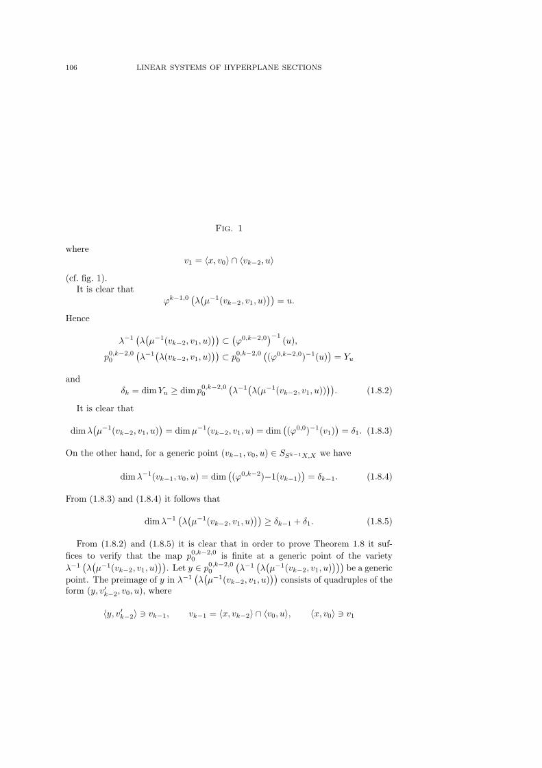
106 LINEAR SYSTEMS OF HYPERPLANE SECTIONS
Fig. 1
wherev1 = 〈x, v0〉 ∩ 〈vk−2, u〉
(cf. fig. 1).It is clear that
ϕk−1,0(λ(µ−1(vk−2, v1, u)
))= u.
Hence
λ−1(λ(µ−1(vk−2, v1, u)
)) ⊂ (ϕ0,k−2,0
)−1(u),
p0,k−2,00
(λ−1
(λ(vk−2, v1, u)
)) ⊂ p0,k−2,00
((ϕ0,k−2,0)−1(u)
)= Yu
andδk = dim Yu ≥ dim p0,k−2,0
0
(λ−1
(λ(µ−1(vk−2, v1, u))
)). (1.8.2)
It is clear that
dim λ(µ−1(vk−2, v1, u)
)= dim µ−1(vk−2, v1, u) = dim
((ϕ0,0)−1(v1)
)= δ1. (1.8.3)
On the other hand, for a generic point (vk−1, v0, u) ∈ SSk−1X,X we have
dim λ−1(vk−1, v0, u) = dim((ϕ0,k−2)−1(vk−1)
)= δk−1. (1.8.4)
From (1.8.3) and (1.8.4) it follows that
dim λ−1(λ(µ−1(vk−2, v1, u)
)) ≥ δk−1 + δ1. (1.8.5)
From (1.8.2) and (1.8.5) it is clear that in order to prove Theorem 1.8 it suf-fices to verify that the map p0,k−2,0
0 is finite at a generic point of the varietyλ−1
(λ(µ−1(vk−2, v1, u)
)). Let y ∈ p0,k−2,0
0
(λ−1
(λ(µ−1(vk−2, v1, u)
)))be a generic
point. The preimage of y in λ−1(λ(µ−1(vk−2, v1, u)
))consists of quadruples of the
form (y, v′k−2, v0, u), where
〈y, v′k−2〉 3 vk−1, vk−1 = 〈x, vk−2〉 ∩ 〈v0, u〉, 〈x, v0〉 3 v1
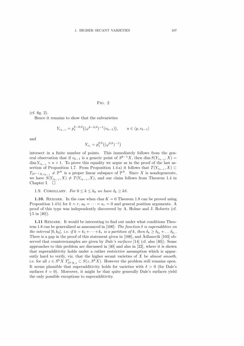
1. HIGHER SECANT VARIETIES 107
Fig. 2
(cf. fig. 2).Hence it remains to show that the subvarieties
Yvk−1 = pk−2,01
((ϕk−2,0)−1(vk−1)
), u ∈ 〈y, vk−1〉
andYv1 = p0,0
1
((ϕ0,0)−1
)
intersect in a finite number of points. This immediately follows from the gen-eral observation that if vk−1 is a generic point of Sk−1X, then dim S(Yvk−1 , X) =dim Yvk−1 + n + 1. To prove this equality we argue as in the proof of the last as-sertion of Proposition 1.7. From Proposition 1.4 a) it follows that T (Yvk−1 , X) ⊂TSk−1X,vk−1
6= PN is a proper linear subspace of PN . Since X is nondegenerate,we have S(Yvk−1 , X) 6= T (Yvk−1 , X), and our claim follows from Theorem 1.4 inChapter I. ¤
1.9. Corollary. For 0 ≤ k ≤ k0 we have δk ≥ kδ.
1.10. Remark. In the case when charK = 0 Theorem 1.8 can be proved usingProposition 1.4 b) for k = r, a0 = · · · = ar = 0 and general position arguments. Aproof of this type was independently discovered by A. Holme and J. Roberts (cf.§ 5 in [40]).
1.11 Remark. It would be interesting to find out under what conditions Theo-rem 1.8 can be generalized as announced in [100]: The function δ is superadditive onthe interval [0, k0], i.e. if k = k1 + · · ·+kr is a partition of k, then δk ≥ δk1 + . . . δkr .There is a gap in the proof of this statement given in [100], and Adlansvik [103] ob-served that counterexamples are given by Dale’s surfaces [14] (cf. also [40]). Someapproaches to this problem are discussed in [40] and also in [22], where it is shownthat superadditivity holds under a rather restrictive assumption which is appar-ently hard to verify, viz. that the higher secant varieties of X be almost smooth,i.e. for all z ∈ SkX T ′SkX,z ⊂ S(z, SkX). However the problem still remains open.It seems plausible that superadditivity holds for varieties with δ > 0 (for Dale’ssurfaces δ = 0). Moreover, it might be that quite generally Dale’s surfaces yieldthe only possible exceptions to superadditivity.
108 LINEAR SYSTEMS OF HYPERPLANE SECTIONS
1.12. Theorem. k0 ≤[
nδ
], i.e. S[n
δ ]X = PN (for δ = 0 the assertion of thetheorem is empty).
Proof. From the definition of k0 (cf. (1.2.2)) it follows that for a ≥ k0 we haveSaX = PN , so that to prove Theorem 1.12 it suffices to verify that n
δ ≥ k0. FromTheorem 1.8 it follows that
δk0 ≥ k0δ, (1.12.1)
and (1.5.6) yieldsδk0 ≤ n. (1.12.2)
Combining (1.12.1) and (1.12.2), we see that k0δ ≤ n (one could also use Theo-rem 1.8 for k = k0 − 1 and the inequality (1.7.1) proved in Proposition 1.7). ¤
Theorem 1.12 allows to give a simple proof of the Hartshorne conjecture on linearnormality (cf. Corollary 2.11 in Chapter II).
1.13. Corollary. If SX 6= PN , then δ ≤ n2 and n ≤ 2
3 (N − 2).
Proof. In fact, for δ > n2 we have
[nδ
]= 1, and from Theorem 1.12 it follows
that SX = PN . Furthermore, if SX 6= PN , then
N ≥ s + 1 = 2n + 2− δ ≥ 3n
2+ 2,
i.e. n ≤ 23 (N − 2). ¤
2. MAXIMAL EMBEDDINGS OF VARIETIES OF SMALL CODIMENSION 109
2. Maximal embeddings of varieties of small codimension
Let X be a nonsingular projective variety over an algebraically closed field K.Projections yield a partial order on the set of all nondegenerate embeddings of Xin projective spaces. Of special interest are maximal and minimal embeddings withrespect to this order.
We denote by M(n, δ) (resp. m(n, δ)) the maximal (resp. minimal) integer N forwhich there exists a nonsingular nondegenerate variety X ⊂ PN such that
dim X = n, δ(X) = δ
(in case there is no finite maximum, we set M(n, δ) = ∞). Ruling out the obviouscase X = Pn, we see that the functions m and M are defined on the set of all pairs(n, δ) ∈ Z2 for which 0 ≤ δ ≤ n and M(n, 0) = ∞.
2.1. Example. Suppose that δ > n2 . Then
M(n, δ) = m(n, δ) = 2n + 1− δ.
In fact, by Corollary 1.13 (or Corollary 2.11 from Chapter II), for δ > n2
SX = PN = 〈X〉
andN = s = 2n + 1− δ = M(n, δ) = m(n, δ).
2.2. Proposition.
(i) m(n, δ) = 2n + 1− δ;(ii) M(n, δ − 1) ≥ M(n, δ) + 1;(iii) M(n− 1, δ − 1) ≥ M(n, δ)− 1
(we assume that all pairs of integers involved in the statement of the proposition liein the domain of definition of the functions m and M).
Proof. (i) In fact, for each X with dim X = n, δ(X) = δ we have
m(n, δ) ≥ sX = 2n + 1− δ. (2.2.1)
Taking X to be the intersection of n + 1− δ generic hypersurfaces
Hi ⊂ P2n+1−δ, deg Hi > 1, i = 1, . . . , n + 1− δ,
we see thatm(n, δ) ≤ 2n + 1− δ. (2.2.2)
Combining (2.2.1) and (2.2.2) we see that (i) holds.(ii) Let X ⊂ PM(n,δ) be a nonsingular nondegenerate variety for which dim X =
n, δ(X) = δ, and let u ∈ PM(n,δ)+1 be a generic point. Consider the projectivecone S(u,X) ⊂ PM(n,δ)+1 with vertex u, and let
X ′ = S(u, X)n+1 ∩HM(n,δ),
110 LINEAR SYSTEMS OF HYPERPLANE SECTIONS
whereH ⊂ PM(n,δ)+1, deg H > 1
is a general hypersurface. Then X ′ is a nonsingular nondegenerate variety, n′ =dim X ′ = dim X = n, and it is easy to see that for δ > 0
SX ′ = S(u, SX), s′ = dim SX ′ = dim SX + 1 = s + 1,
andδ′ = δ(X ′) = 2n′ + 1− s′ = 2n− s = δ − 1,
which proves (ii).(iii) Let X ⊂ PM(n,δ) be a nonsingular nondegenerate variety for which dim X =
n, δ(X) = δ, and letX ′ = X ∩H ⊂ PM(n,δ)−1
be the intersection of X with a generic hyperplane H ⊂ PM(n,δ). Then X ′ is anonsingular nondegenerate variety, n′ = dim X ′ = dim X − 1 = n− 1, and it is nothard to see that for δ > 0
SX ′ = SX ∩H, s′ = dim SX ′ = dim SX − 1 = s− 1
andδ′ = δ(X ′) = 2n′ + 1− s′ = 2n− s = δ − 1.
Assertion (iii) and Proposition 2.2 are proved. ¤2.3. Theorem. M(n, δ) ≤ f
([nδ
])= n(n+δ+2)
2δ + 12
nδ
(δ − δ
nδ
− 2)
=n(n+δ+2)+ε(δ−ε−2)
2δ , where f(k) = (k + 1)(n + 1) − k(k+1)2 δ − 1, ε = δ
nδ
= n
(mod δ),[
nδ
]is the largest integer not exceeding n
δ , and
nδ
= n
δ −[
nδ
].
Proof. Let X ⊂ PM(n,δ) be a nonsingular nondegenerate variety, dimX = n,δ(X) = δ. From (1.5.8) and Corollary 1.9 it follows that for k ≤ k0
sk = (k + 1)(n + 1)−k∑
i=1
δi − 1 ≤ (k + 1)(n + 1)−k∑
i=1
i δ − 1 = f(k). (2.3.1)
The graph of the function f(k) is a parabola (cf. fig. 3); f attains maximal value(equal to (2n+δ+2)2
8δ − 1) for k = 2n−δ+22δ = a, and f is a monotone increasing
function for 0 ≤ k ≤ a.
Fig. 3
2. MAXIMAL EMBEDDINGS OF VARIETIES OF SMALL CODIMENSION 111
From (1.2.2) and (2.3.1) it follows that
M(n, δ) = sk0 ≤ f(k0), (2.3.2)
and from Theorem 1.12 it follows that k0 ≤[
nδ
]. If k0 <
[nδ
], then
k0 ≤[n
δ
]− 1 ≤ n
δ− 1 < a
andf(k0) ≤ f
(n
δ− 1
)= f
(n
δ
)− 1 < f
([n
δ
])(2.3.3)
(we observe that from (2.3.1) it follows that f([
nδ
])is an integer). From (2.3.2)
and (2.3.3) it follows that we always have
M(n, δ) ≤ f([n
δ
]),
and to prove Theorem 2.3 it remains to explicitly compute f([
nδ
]). ¤
2.4. Remark. Proposition 2.2 (i) and Theorem 2.3 show that for δ(X) = δ > 0the dimension N of the linear span of Xn (n ≥ δ − 1) lies in the limits depicted infig. 4.
Fig. 4
112 LINEAR SYSTEMS OF HYPERPLANE SECTIONS
2.5. Remark. If δ > n2 , then
[nδ
]= 1, f
([nδ
])= 2n + 1− δ, and Theorem 2.3
shows that
M(n, δ) = m(n, δ) = 2n + 1− δ ≤ 3n + 12
(cf. also Corollary 1.13).
2.6. Remark. For δ = n2
(n ≡ 0 (mod 2)
)Theorem 2.3 yields:
N ≤ f([n
δ
])= f(2) =
3n
2+ 2.
Here there are two possibilities:
(i) SX = PN , N = s = m(n, n
2
)= 3n
2 + 1;(ii) SX 6= PN , N = s + 1 = M
(n, n
2
)= f(2) = 3n
2 + 2.
Nonsingular nondegenerate varieties Xn ⊂ PN for which N > s = 3n2 +1 are called
Severi varieties (cf. Definition 1.2 in Chapter IV). Thus (ii) means that each Severivariety lies in a
(3n2 + 2
)-dimensional projective space. Of course, this also follows
from classification of Severi varieties (cf. Theorem 4.7 in Chapter IV).
2.7. Remark. From Remark 2.5 it follows that if
SXn 6= PN , n ≡ 1 (mod 2),
then
δ ≤ n− 12
, s = 2n + 1− δ ≥ 3n + 32
.
Consider the extremal case when δ = n−12 . By Theorem 2.3, for n = 3 (δ = 1) we
have
N ≤ n(n + 3)2
= 9 = s + 3,
and for n > 3
N ≤ 3n(n + 1)2(n− 1)
+12· 2n− 1
(n− 1
2− n− 1
2· 2n− 1
− 2)
=3n + 7
2= s + 2.
Thus if n ≡ 1 (mod 2), δ = n−12 , then there are the following possibilities:
(i) SX = PN , N = s = m(n, n−1
2
)= 3n+3
2 ;(ii) N = s + 1 = 3n+5
2 ;(iii) N = s + 2 = 3n+7
2
(= M
(n, n−1
2
)if n > 3
);
(iv) n = 3, N = s + 3 = M(3, 1) = 9.
All these cases really occur: as an example of case (ii) one can take a nonsingularhyperplane section of any of the Severi varieties; an example of case (iii) is givenby the five-dimensional Segre variety P2 × P3 ⊂ P11, and an example of case (iv)is given by the Veronese variety v2(P3 ⊂ P9 (cf. [77] and [24], where all threefoldsX3 ⊂ PN with δ = 1 and SX 6= PN are classified; cf. also Remark 2.9).
2. MAXIMAL EMBEDDINGS OF VARIETIES OF SMALL CODIMENSION 113
2.8. Definition. Nonsingular nondegenerate varieties Xn ⊂ PN for whichδ(X) = δ > 0 and N = M(n, δ) will be called extremal varieties.
2.9. Remark. The bound in Theorem 2.3 is sharp. Examples of extremalvarieties Xn ⊂ PN for which
N = M(n, δ) = f([n
δ
])(2.9.1)
are given by all varieties with δ > n2 (cf. Remark 2.5), by the Severi varieties (δ = n
2 ;cf. Remark 2.6 and Theorem 4.7 in Chapter IV), by the Veronese varieties
v2(Pn) ⊂ Pn(n+3)2 (δ = 1),
by the Segre varieties
Pa × Pb ⊂ P(a+1)(b+1)−1, |a− b| ≤ 1 (δ = 2),
and by the Grassmann varieties
G(m, 1) ⊂ P (m+12 )−1, (δ = 4).
In Chapter VI we shall show that each variety Xn ⊂ PN satisfying condition (2.9.1)(i.e. such that the inequality in Theorem 2.3 turns into equality) coincides with oneof the varieties listed in this remark (cf. Theorem 5.6 in Chapter VI). We remarkthat from the proof of Theorem 2.3 it follows that for an extremal variety Xn ⊂PM(n,δ), δ = δ(X) M(n, δ) = f
([nδ
])if and only if k0 =
[nδ
]and the inequalities
(2.3.1) turn into equalities for all k ≤ k0, i.e. δi = iδ for 0 ≤ i ≤ k0 =[
nδ
](cf.
Proposition 1.2 in Chapter VI).
2.10. Theorem. Let Xn ⊂ Pr be a (not necessarily nondegenerate) nonsingularvariety. Then the dimension of the complete linear system of hyperplane sectionsof X does not exceed f
([n
2n+1−r
]), where f is the function defined by (2.3.1). In
other words,
h0(X,OX(1)) ≤ f
([n
2n + 1− r
])+ 1 ≤
[(4n− r + 3)2
8(2n− r + 1)
].
Proof. Let X ⊂ PN be the image of X under the embedding defined by thecomplete linear system |OX(1)|, N = h0(X,OX(1))− 1. Then
δ = δ(X) = 2n + 1− s = 2n + 1− s ≥ 2n + 1− r
n = dim X = n, s = dim SX = dim SX = s.
By Proposition 2.2 (ii),
N ≤ M(n, δ) ≤ M(n, 2n + 1− r). (2.10.1)
114 LINEAR SYSTEMS OF HYPERPLANE SECTIONS
From (2.10.1) and Theorem 2.3 it follows that
h0(X,OX(1)) ≤ f
([n
2n + 1− r
])+ 1. (2.10.2)
On the other hand, it is not hard to see that, for fixed n and r, the second term inthe expression
f
([n
2n + 1− r
])=
n(3n− r + 3)2(2n− r + 1)
+ε(2n− r − ε− 1)
2(2n− r + 1)
attains maximal value equal to (2n−r−1)2
8(2n−r+1) for ε = 2n−r−12 . Hence
f
([n
2n + 1− r
])+ 1 ≤ n(3n− r + 3)
2(2n− r + 1)+
(2n− r − 1)2
8(2n− r + 1)+ 1 =
(4n− r + 3)2
8(2n− r + 1).
(2.10.3)Theorem 2.10 immediately follows from (2.10.2) and (2.10.3). ¤
2.11. Definition. Let Xn ⊂ Pr be a nonsingular nondegenerate variety. Thevariety Xn ⊂ PN , N = h0(X,OX(1)) − 1 defined as the image of X under theembedding given by the complete linear system |OX(1)| will be called the linearnormalization of X .
2.12. Corollary. Let Xn ⊂ Pr, r ≤ 2n be a nonsingular variety. Thenh0(X,OX(1)) ≤ (
n+22
). In other words, if codimPr X ≤ dim X and X is the linear
span of X, then dim 〈X〉 ≤ n(n+3)2 .
Proof. Since in the statement of Theorem 2.10 X is not supposed to be non-degenerate, we may assume that r = 2n. In this case Corollary 2.12 immediatelyfollows from Theorem 2.10 because
f(n) =n(n + 3)
2=
(n + 2
2
)− 1.
¤2.13. Remark. In the case when X is a complex manifold and
r = s(X) = dim SX = dim TX = 2n
Corollary 2.12 was proved in [28, 6.16] by completely different (analytic) methods.
2.14. Remark. If for a nonsingular variety Xn ⊂ P2n we have h0(X,OX(1)) =(n+2
2
), then X ' Pn and the embedding Pn → P2n is defined by a generic collection
of 2n + 1 quadratic forms (cf. Remark 2.9 and Corollary 2.9 in Chapter VI).
2.15. Remark. It is clear that for r > 2n the dimension h0(X,OX(1)) canassume arbitrarily large values: it suffices to take a nonsingular linearly normalvariety X ⊂ PN , N ≥ r (dim X = n, h0(X,OX(1)) = N + 1) and to project itisomorphically to Pr; the image of X under this projection is a nonsingular varietyX ⊂ Pr for which dim X = n and h0(X,OX(1)) = N +1. This is only a restatementof the fact that M(n, 0) = ∞.
It is convenient to interpret Theorem 2.10 using the notion of abnormality index.
2. MAXIMAL EMBEDDINGS OF VARIETIES OF SMALL CODIMENSION 115
2.16. Definition. Let Xn ⊂ Pr be a nonsingular nondegenerate variety, andlet X ⊂ PN be the linear normalization of X. The number λ(X) = N − r =h0(X,OX(1)) − r − 1 is called the (linear) abnormality index of the projectivevariety X.
It is clear that linearly normal varieties have abnormality index zero; if δ > 0,then curves have abnormality index zero, the abnormality index of surfaces doesnot exceed one, and the abnormality index of threefolds lies in the interval betweenzero and three (cf. Remarks 2.5–2.7).
Theorem 2.10 can be restated as follows.
2.17. Corollary. For a nonsingular nondegenerate variety Xn with s(X) ≤ sthe following inequality holds:
λ(X) ≤ (2s− 3n)(s− n− 1)2(2n− s + 1)
+ε(2n− s− ε− 1)
2(2n− s + 1)=
(2s− 3n)(s− n− 1)2(2n− s + 1)
+(n− s + 1
2
)n
2n− s + 1
−
(n− s− 1
2
)n
2n− s + 1
2
,
where ε = n (mod 2n− s+1). In particular, if s(X) ≤ 2n (or, which is equivalent,SX = TX cf. Theorem 1.4 in Chapter I ), then λ(X) ≤ n(n−1)
2 .
CHAPTER VI
SCORZA VARIETIES
Typeset by AMS-TEX
116
1. PROPERTIES OF SCORZA VARIETIES 117
1. Properties of Scorza varieties
1.1. Definition. Let Xn ⊂ PN be a nonsingular nondegenerate variety. Wecall X a Scorza variety if, in the notations of Chapter V,
(i) N > m(n, δ), where δ = δ(X) = 2n + 1− s;(ii) N = M(n, δ) < ∞, i.e. δ > 0 and X is an extremal variety in the sense of
Definition 2.8 from Chapter V;(iii) M(n, δ) = f
([nδ
])= n(n+δ+2)+ε(δ−ε−2)
2δ , where f is the function defined byformula (2.3.1) from Chapter V (i.e. f(k) = (k + 1)(n + 1)− k(k+1)
2 δ − 1)and ε = n (mod δ).
By Proposition 2.2 from Chapter V, condition (i) is equivalent to condition(i′) SX 6= PN .
From Theorem 2.3 in Chapter V it follows that
(ii) & (iii) ⇔ (iv):
(iv) N = f([
nδ
]).
Finally, from the definition of f it follows that for 1 ≤ δ ≤ n2
(iv) ⇒ (i′)
(for δ > n2 we have f
([nδ
])= f(1) = m(n, δ) = M(n, δ); cf. Remark 2.5 in
Chapter V).Thus X is a Scorza variety if and only if n ≥ 2δ > 0, N = f
([nδ
]).
Scorza varieties are named in memory of the Italian mathematician Guido Scorzawho obtained pioneer results in the study of linear normalizations of varieties ofsmall codimension (cf. [77; 78]).
The goal of the present chapter is to give classification of Scorza varieties.Throughout this chapter we consider varieties defined over an algebraically closedfield K, charK = 0.
1.2. Proposition. Let Xn ⊂ PN be a nonsingular nondegenerate variety, andlet δ(X) = δ ≤ n
2 . Consider the following conditions:(a) X is a Scorza variety;(b) k0 =
[nδ
](where k0 = min k|SkX = PN);
(c) δi = iδ for 0 ≤ i ≤ [nδ
](where δi is defined by formula (1.5.2) in Chap-
ter V).Then (a) ⇔ (b) & (c). Furthermore, (b) ⇒ (c) for n ≡ 0 (mod δ) and
(c) ⇒ (b) for n 6≡ 0 (mod δ).
Proof. The equivalence (a) ⇔ (b) & (c) immediately follows from the proof ofTheorem 2.3 in Chapter V (cf. Remark 2.9 in Chapter V).
Suppose that n ≡ 0 (mod δ) and that condition (b) holds. By Theorem 1.8 inChapter V,
iδ ≤ δi ≤ δk0 − (k0 − i)δ ≤ n− (k0 − i)δ = iδ 0 ≤ i ≤ n
δ,
118 VI. SCORZA VARIETIES
i.e. δi = iδ for 0 ≤ i ≤ nδ . Hence for n ≡ 0 (mod δ) we have (b) ⇒ (c) and
(a) ⇔ (b).Suppose now that n 6= 0 (mod δ) and that condition (c) holds. Then δk0+1 =
n >[
nδ
]. Hence k0 + 1 >
[nδ
]and k0 ≥
[nδ
]. On the other hand, by Theorem 1.12
in Chapter V we have k0 ≤[
nδ
]. Hence k0 =
[nδ
], i.e. for n 6≡ 0 (mod δ) we have
(c) ⇒ (b) and (a) ⇔ (c). ¤
1.3. Remark. If n 6≡ 0 (mod δ), then in general (b) 6⇒ (a). An example is givenby the projection of Segre variety Pm × Pm+1 ⊂ Pm2+3m+1 from a generic pointu ∈ Pm2+3m+1. We denote this variety by X. Then
n = 2m + 1, N2 = m2 + 3m, δ = 2, δi = 2i, 0 ≤ i < m, k0 = m,
butδm = 2m + 1, N = f
([n
2
])− 1.
If n ≡ 0 (mod δ), then in general (c) 6⇒ (a). An example is given by an arbitraryvariety Xn ⊂ P 3n
2 +1. In this case
δ =n
2, δ2 = n,
but Remark 2.6 from Chapter V shows that
k0 = 1, N = f(2)− 1.
1.4. Theorem. Let Xn ⊂ PN , N = f([
nδ
]), δ = δ(X) be a Scorza variety, and
let u be a general point of SkX, 2 ≤ k ≤ k0 − 1 (by Proposition 1.2, k0 =[
nδ
]).
Then in the notations of Chapter V (cf. Chapter V, (1.5.1), (1.5.2), and (2.3.1)),Yu ⊂ Pu is a Scorza variety, where
Pu =u′ ∈ SkX
∣∣ TSkX,u′ = TSkX,u
= SkYu,
and we have
dim Yu = kδ, k0(Yu) = k, δi(Yu) = iδ, 0 ≤ i ≤ k, dimPu = f(k).
If k = k0 ≥ 2, then Yu is a Scorza variety of dimension k0δ = n − ε, δ = δ(Yu) inthe projective space Pu = 〈Yu〉 = Sk0Yu, dimPu = f(k0).
Proof. From Proposition 1.2 (c) and usual general position arguments it followsthat for a generic point u ∈ SkX, 0 ≤ k ≤ k0 the variety Yu is nonsingular andhas dimension kδ. Arguing by descending induction on k, we see that it suffices toprove Theorem 1.4 in the cases k = k0 − 1 (k0 ≥ 3) and k = k0.
First we consider the case
k = k0 − 1, dim Yu = (k0 − 1)δ.
1. PROPERTIES OF SCORZA VARIETIES 119
Since for k0 ≥ 3 we have (k0 − 1)δ ≥ 2δ, from Proposition 1.2((b) ⇒ (a) for n ≡ 0
(mod δ))
it follows that to show that Yu is a Scorza variety it suffices to verify that
δ(Yu) = δ, k0(Yu) =[dim Yu
δ
]= k0 − 1. (1.4.1)
Let
Lu = TSk0−1X,u, dim Lu = sk0−1 = N − 1− (n− δk0(X)
)= N − ε− 1,
where ε = n− δk0(X) = n− k0δ (cf. formula (1.5.4) in Chapter V). Put
YLu=
x ∈ X
∣∣ TX,x ⊂ Lu
.
By Proposition 1.4 a) from Chapter V
Yu ⊂ YLu (1.4.2)
Projecting X to Ps (s = 2n + 1 − δ) from a general (N − s − 1)-dimensionallinear subspace of Lu and applying the theorem on tangencies (cf. Corollary 1.8 inChapter I), we see that
dim YLu ≤ (s− ε− 1)− n− 1 = n− δ − ε = (k0 − 1)δ = dim Yu. (1.4.3)
From (1.4.2) and (1.4.3) it follows that Yu is a component of YLu . Varying u, wesee that for a generic point u′ ∈ Sk0−1Yu
Yu′ = Yu (1.4.4)
(Yu′ ⊂ YLu′ = YLu in view of Proposition 1.4 in Chapter V). From (1.4.4) it followsthat for a generic collection of k points
(y0, . . . , yk−1), yi ∈ Yu, 0 ≤ i ≤ k − 1, k ≤ k0
and a generic point v ∈ 〈y0, . . . , yk−1〉 we have Yv ⊂ Yu. In particular, for k = 2from this it follows that
δ(Yu) ≥ δ(X) = δ. (1.4.5)
Since u is a generic point of Sk0−1X,
δ(Yu) ≤ δ (1.4.6)
Combining (1.4.5) and (1.4.6) we conclude that
δ(Yu) = δ (1.4.7)
which proves the first of the equalities (1.4.1).The fact that
Pu =u′ ∈ Sk0−1X
∣∣ TSk0−1X,u′ = Lu
120 VI. SCORZA VARIETIES
is a linear subspace immediately follows from the reflexivity theorem of C. Segre(cf. e.g. [49; 50]). From Proposition 1.4 b) in Chapter V it follows that
Yu ⊂ Sk0−1Yu ⊂ Pu.
On the other hand, assertion a) of the same proposition shows that for a genericpoint u′ ∈ Pu
Yu′ ⊂ YLu. (1.4.8)
Since Yu is irreducible, from (1.4.3) and (1.4.8) it follows that
Sk0−1Yu = Pu. (1.4.9)
It remains to show that k0(Yu) = k0 − 1 (this is the second of the inequalities(1.4.1)) and dimPu = f(k0− 1). In view of Proposition 1.2, to do this it suffices toverify that
SkYu 6= Pu, k < k0 − 1. (1.4.10)
But (1.4.10) immediately follows from the fact that u is a generic point of Sk0−1X,so that u ∈ Pu \ SkX for k < k0. Thus Theorem 1.4 holds for k = k0 − 1 andtherefore for all 2 ≤ k ≤ k0 − 1. We observe that the same argument shows thatequalities (1.4.1) also hold for k = 1, so that for a generic point z ∈ SX the varietyYz is nonsingular,
dim Yz = δ(Yz) = δ, SYz = Pz =z′ ∈ SX
∣∣ TSX,z′ = TSX,z
(1.4.11)
(from (1.4.11) it immediately follows that Yz is a hypersurface).Now we consider the case k = k0. To prove (1.4.7) it suffices to verify that for
a generic point u ∈ Sk0X = PN , a generic pair of points x, y ∈ Yu, and a genericpoint z ∈ 〈x, y〉 we have Yz ⊂ Yu. Consider the morphism
ϕ1,k0 : SSX,Sk0−2X → PN
(cf. §1 of Chapter V) and put
Y 1u = p1,k0−2
1
((ϕ1,k0−2)−1(u)
).
From 1.2 (c) and formula (1.5.4) in Chapter V it follows that
dim Y 1u = (s1 + sk0−2 + 1)− sk0
= (2n + 2− δ) + sk0−2 − (sk0−1 + n + 1− δk0)
= (2n + 2− δ)− [(sk0−2 + n + 1− δk0−1) + (n + 1− δk0)]
= δk0−1 + δk0 − δ = 2(k0 − 1)δ. (1.4.12)
From (1.4.12) it follows that
dim Y 1u + 2δ = 2 dim Yu,
and hence there exists a point z ∈ Y 1u such that x, y ∈ Yz ⊂ Yu. Furthermore, it is
clear that z is a generic point of Pz, and from (1.4.11) it follows that Yz = Yz ⊂ Yu
which implies (1.4.7). From the already established part of Theorem 1.4 it followsthat
k0(Yu) = k0(X) = k0 =dim Yu
δ.
Hence Proposition 1.2((b) ⇒ (a) for n ≡ 0 (mod δ)
)shows that Yu is a Scorza
variety. ¤
1. PROPERTIES OF SCORZA VARIETIES 121
1.5. Corollary. Let Xn ⊂ PM(n,δ), δ = δ(X) be a Scorza variety. Then for ageneric point z ∈ SX the variety Yz is a nonsingular δ-dimensional quadric.
Proof. In the proof of Theorem 1.4 it was shown that for a generic point z ∈ SXthe variety Yz is a nonsingular hypersurface in Pz = SYz = Pδ+1 (cf. (1.4.11)).Since X is not a hypersurface, a generic secant intersects X at exactly two points(cf. [34, Chapter IV, §3; 39, 2.5; 64, §7B]) which proves Corollary 1.5 (in viewof Proposition 2.1 in Chapter IV, Corollary 1.5 also follows from Corollary 1.6below). ¤
1.6. Corollary. Let Xn ⊂ PM(n,δ), δ = δ(X) be a Scorza variety. Then δ = 1,2, 4, or 8, and if u ∈ S2X is a generic point, then Yu is a Severi variety (cf.Definition 1.2 in Chapter IV).
Proof. From Theorem 1.4 it follows that Yu is an extremal variety,
dim Yu = 2δ, δ(Yu) = δ, dim 〈Yu〉 = f(2) = 3δ + 2. (1.6.1)
From Remark 2.6 in Chapter V it follows that Yu is a Severi variety. In view ofTheorem 3.10 in Chapter IV, from (1.6.1) it follows that δ = δ(Yu) can assume onlyfour values indicated in the statement of the corollary. ¤
Corollary 1.6 shows that for classification of Scorza varieties it suffices to considerfour cases, viz. δ = 1, 2, 4, 8. This will be done in the next four sections.

122 VI. SCORZA VARIETIES
2. Scorza varieties with δ = 1
The goal of the present section is to give a proof of the following main result.
2.1. Theorem. Let Xn ⊂ PN , n ≥ 2 be a nonsingular nondegenerate varietysuch that sX ≤ 2n (by Theorem 1.4 of Chapter I, this condition holds if and only
if SX = TX). Then N ≤ n(n+3)2 and equality holds if and only if X = v2(Pn) ⊂
Pn(n+3)
2 is the Veronese variety.
In particular, M(n, 1) = n(n+3)2 and the Veronese variety is the only Scorza
variety of dimension n with δ = 1.
Proof. The inequality N ≤ n(n+3)2 was already proven in Corollary 2.12 in Chap-
ter V.Suppose that N = f(n) = n(n+3)
2 . From Proposition 2.2 in Chapter V it followsthat that δ = 1. We start with the following general result which holds for all δ.
2.2. Lemma. Let Xn ⊂ PM(n,δ), δ = δ(X) > 0 be a Scorza variety. Supposethat n ≡ 0 (mod δ) so that M(n, δ) = f(k0), k0 = n
δ , and let u ∈ Sk0−1X and
z ∈ SX be generic points. Then sk0−1 = N − 1 and(Y δ
z · Y n−δu
)= 1.
Proof of Lemma 2.2. From Proposition 1.2 (c) and formulas (1.5.6) and (1.5.7)in Chapter V it follows that
n = δk0 = k0δ, sk0−1 = sk0 − (n + 1− δk0) = N − 1.
From (1.4.2) it follows that
T (Yu, X) ⊂ Lu = TSk0−1X,u. (2.2.1)
Since X is a nondegenerate variety, from (2.2.1) and Theorem 1.4 of Chapter I itfollows that
dim S(Yu, X) = dim Yu + n + 1 = 2n + 1− δ = s. (2.2.2)
Equality (2.2.2) means thatS(Yu, X) = SX (2.2.3)
(similarly, one can show that S(Yz, Sk0−2X) = Sk0−1X). From (2.2.3) it follows
thatYz ∩ Yu 6= ∅. (2.2.4)
In view of Corollary 1.5, Y δz ⊂ Pδ+1
z = SYz is a nonsingular quadric. Since Lu 6⊃ Pz,Lu ∩ Pz is a hyperplane in Pz which is tangent to Yz at all points of Yz ∩ Yu. Fromthis and (2.2.4) it immediately follows that (Yz · Yu) = 1.
Lemma 2.2 is proved.
We return to the case δ = 1. In this case (2.2.1) means that Lu ·X = rYu + Eu,where r ≥ 2, Yu 6⊂ SuppEu. From Lemma 2.2 it follows that
2 = deg Yz = (Lu · Yz) = r + (Eu · Yz). (2.2.5)
Formula (2.2.5) shows that
r = 2, (Eu · Yz) = 0. (2.2.6)
2. SCORZA VARIETIES WITH δ = 1 123
2.3. Lemma. In the assumptions of Theorem 2.1, for a generic point u ∈Sn−1X we have Eu = 0.
Proof of Lemma 2.3. First we observe that if Eu 6= 0, then Eu = E is the fixedpart of the algebraic system Lu ·X, where u runs through the set of generic pointsof Sn−1X. In fact, if this were not so, then Eu would contain a generic point x ∈ X,and if x′ is another generic point of X and z is a generic point of the line 〈x, x′〉,then Yz would intersect the divisor Eu at a finite set of points. Since x ∈ Yz ∩ Eu,this set is non-empty contrary to (2.2.6).
Lemma 2.3 now follows from the following result.
2.4. Lemma. Let Xn ⊂ PM(n,δ), δ = δ(X) > 0 be a Scorza variety. Then thealgebraic system of divisors Hu = (Lu ·X)PN , Lu = TSk0−1X,u, u ∈ Sk0−1X doesnot have fundamental points on X.
Proof of Lemma 2.4. Suppose the converse, and let y be a fundamental point.Then
y ∈⋂
u∈Sk0−1X
TSk0−1X,u,
and therefore Sk0−1X is a cone with vertex y. Hence Lemma 2.4 is a consequenceof the following result.
2.5. Lemma. Let Xn ⊂ PM(n,δ), δ = δ(X) > 0 be a Scorza variety. ThenSk0−1X is not a cone.
Proof. We prove the lemma by induction. If n = 2δ, then X is a Severi varietyand Lemma 2.5 follows from results of Chapter IV. Using Theorem 1.4, supposethat for a generic point u ∈ Sk0−1X the variety Sk0−2Yu is not a cone and thevariety Sk0−1X is a cone with vertex v. Let u′ be a generic point of the line 〈v, u〉.Then
u′ ∈ Sk0−1X, Lu′ = TSk0−1X,u′ = TSk0−1X,u = Lu
and hence Yu′ = Yu (cf. (1.4.4)). For a generic point x ∈ Yu, we consider the curve
Cv,x,u = p0,k0−21
((p0,k0−2 × ϕ0,k0−2
)−1(x× 〈v, u〉0)
)⊂ Sk0−2Yu (2.5.1)
in the planeΠ = 〈v, x, u〉 ⊂ Sk0−1Yu, (2.5.2)
where 〈v, u〉0 denotes the set of generic points of the line 〈v, u〉. Since sk0−2 ≤sk0−1 − 2 (cf. formula (1.5.4) in Chapter V), we may assume that
〈v, u〉 ∩ Sk0−2Yu = 〈v, u〉 ∩ Sk0−2X = v. (2.5.3)
From (2.5.1) and (2.5.3) it follows that 〈v, u〉 ∩ Cv,x,u = v, and since u is a genericpoint of Π, Cv,x,u consists of several lines passing through v. Hence for a genericpoint w ∈ Sk0−2
u we have 〈v, w〉 ⊂ Sk0−2Yu, i.e., contrary to our assumption,Sk0−2Yu is a cone with vertex v.
This contradiction proves Lemma 2.5 and therefore also Lemmas 2.4 and 2.3.
124 VI. SCORZA VARIETIES
From Lemma 2.3 it follows that
Lu ·X = 2Yu, (2.5.4)
so that in particular Yu is an ample divisor on X. Now it is easy to prove The-orem 2.1 by induction on n using Theorem 1.4, Corollary 1.6, the classical resultof Severi for n = 2 (cf. [82, no 8] or Theorem 4.7 a) in Chapter IV), and the wellknown theorem to the effect that if a nonsingular variety Xn, n > 2 contains anample divisor Y ' Pn−1, then X ' Pn (cf. [63]). However we give a direct proof ofTheorem 2.1.
From (2.5.4) it follows that the image of the rational map
Sn−1 99K Pic0 X, u 7→ cl (Yu − Yu0)
(where u0 is a fixed generic point of Sn−1X) is contained in the set of points oforder two on the Picard variety. Since Sn−1X is an irreducible variety, from this itfollows that for generic points u, u′ ∈ Sn−1X we have Yu ∼ Yu′ (where ∼ denoteslinear equivalence).
Consider the complete linear system of divisors H = |Yu| on the variety X. Weobserve that a general divisor H ∈ H has the form
H = Yu, u ∈ Sn−1X. (2.5.5)
In fact, let x0, . . . , xn−1 ∈ H be a generic collection of n points, and let u ∈〈x0, . . . , xn−1〉 be a generic point. Then it is clear that u is a generic point ofSn−1X, and from Proposition 1.4 b) of Chapter V it follows that
Lu = 〈TX,x0 , . . . , TX,xn−1〉. (2.5.6)
On the other hand, since X is an extremal variety, X is linearly normal, andtherefore the divisor 2H ∼ 2Yu is cut by a hyperplane LH ⊂ PN , i.e. 2H = LH ·X.Hence T (H, X) ⊂ LH , so that from (2.5.6) it follows that
LH = Lu, 2H = LH ·X = Lu ·X = 2Yu,
and H = Yu as stated in (2.5.5).From Lemma 2.4 it follows that the linear system H does not have fundamental
points and hence defines a morphism
h : X → PdimH. (2.5.7)
From (1.4.3) and (2.5.5) it follows that
dimH = dim (Sn−1X)∗ = dim (X × · · · ×X︸ ︷︷ ︸n
)− dim (Yu × · · · × Yu︸ ︷︷ ︸n
) = n. (2.5.8)
Since in view of (2.5.4) the linear system H is ample, (2.5.7) and (2.5.8) show thath : X → Pn is a finite covering.
2. SCORZA VARIETIES WITH δ = 1 125
The preimage of the linear system of quadrics in Pn with respect to the morphismh is a linear subsystem of the complete linear system |2Yu| = Lu · X on X, andsince
N + 1 = h0(X,OX(1)
)= h0
(Pn,OPn(2)
)=
(n + 2
2
)
these two linear systems coincide with each other. Hence h is an isomorphism,h−1 = v2 and X = v2(Pn). ¤
2.6. Remark. For n = 1 we have k0 = 1, so that each plane curve is extremal,i.e. M(1, 1) = m(1, 1) = 2.
2.7. Remark. As we already pointed out, Theorem 2.1 was first proved by Severi[82, no8] (cf. Remark 4.11 in Chapter IV) for n = 2. Adlandsvik independentlyproved a theorem related to Theorem 2.1 to the effect that if sX ≤ 2n and Sn−1Xis not a cone (the last condition is quite hard to verify), then X is a Veronese variety(cf. [103]).
2.8. Remark. It is clear that the morphism (2.5.7) is also defined by the linearsystem |Yu0+H|, where u0 is a fixed generic point of Sn−1X, i.e. by the linear systemof hyperplane sections of X passing through the linear subspace 〈Yu0〉. Hence h isinduced by projecting from the subspace 〈Yu0〉, where
dim 〈Yu0〉 = N − n− 1 =(n− 1)(n + 2)
2= f(n− 1).
In fact, the map inverse to the Veronese mapping
v2 : Pn → v2(Pn) ⊂ Pn(n+3)2
is defined by projecting from the linear subspace
〈v2(Pn−1)〉 = P(n−1)(n+2)
2 ⊂ Pn(n+3)2
(cf. Chapter III, § 3).
2.9. Corollary. Let Xn ⊂ Pr be a nonsingular variety, r ≤ 2n. Then
h0(X,OX(1)
) ≤ (n+2
2
)=
[(n+ 3
2 )2
2
]with equality holding if and only if r = 2n
and either n = 1 or X → P2n is the embedding of the projective space Pn ' Xdefined by a collection of 2n + 1 quadratic forms Q0, . . . , Q2n on Pn.
126 VI. SCORZA VARIETIES
3. Scorza varieties with δ = 2
In this section we prove the following result.
3.1. Theorem. Let Xn ⊂ PN , n ≥ 4 be a nonsingular nondegenerate variety.Suppose that sX < 2n. Then
N ≤ m(m + 2) = (m + 1)2 − 1 for n = 2m ≡ 0 (mod 2),
N ≤ (m + 1)(m + 2)− 1 for n = 2m + 1 ≡ 1 (mod 2).
Furthermore, the inequalities turn into equalities if and only if X = Pm × Pm ⊂Pm(m+2) or X = Pm × Pm+1 ⊂ Pm2+3m+1 is a Segre variety.
In particular, M(n, 2) = n(n+4)−nmod24 and the Segre variety P
n−nmod22 ×Pn+nmod2
2
is the only n-dimensional Scorza variety with δ = 2.
Proof. The inequality
N ≤ f([n
2
])=
n(n + 4)− n mod 24
splitting into the pair of inequalities given in the statement of the theorem followsfrom Proposition 2.2 (ii) and Theorem 2.3 in Chapter V.
Suppose that N = f([
n2
]). From Proposition 2.2 in Chapter V it follows that
δ = 2. Proposition 1.2 shows that
k0 =[n
2
]= m, δk = 2k, 0 ≤ k ≤ m.
Suppose first that n = 2m. By Lemma 2.2, sm−1 = N−1, and for a generic pointu of the hypersurface Sm−1X ⊂ PN (N = m(m+2)) the hyperplane Lu = TSm−1X,u
is tangent to X along Yu, codimX Yu = 2. Furthermore, for a generic point z ∈ SXwe have (Yu · Yz) = 1. Put Hu = Lu ·X. For a generic point y ∈ Yu and a genericpoint z ∈ SyX
(Yz ·Hu)X = (Yz · Lu)PN = (Yz · TYz,y)P3z
(here, according to Corollary 1.5, Yz is a nonsingular two-dimensional quadric),Pz = 〈Yz〉. Thus
(Yz ·Hu)X = lz1 ∪ lz2,
where lz1, lz2 is a pair of lines intersecting at y. If z′ is another generic point of SyXand
(Yz′ ·Hu)X = (Yz ·Hu)X , (3.1.1)
then it is clear that Yz′ = Yz, so that z′ ∈ P3z. Varying z in the set of general points
of the cone SyX, we obtain a (dim SyX − dimP3z)=(n − 2)-dimensional family of
pairs of lines lz1, lz2 ⊂ Hu such that
lz1 ∩ Yu = lz2 ∩ Yu = (lz1 · lz2)Y = y.
3. SCORZA VARIETIES WITH δ = 2 127
Furthermore, we may assume that the pairs (lz1, lz2) are ordered so that the lines lz1
(resp. lz2), z ∈ SyX form an irreducible family Fy1 (resp. Fy
2 ) of lines in Hu passingthrough y.
For generic lines l1 ∈ Fy1 , l2 ∈ Fy
2 we have
l1 ∩ l2 = (Yz ·Hu)X ,
where z is a generic point of the plane 〈l1, l2〉. Hence the dimension of the familiesFy
1 and Fy2 is equal to 1
2 (n−2) = m−1, and the closure of the subset of the divisorHu swept out by the lines lz1 (resp. lz2) is an irreducible m-dimensional cone Cy
1
(resp. Cy2 ) with vertex y.
Varying y in the set of generic points of Yu, we obtain two irreducible subvarieties
Cu1 =
⋂
y∈Yu
Cy1 , Cu
2 =⋂
y∈Yu
Cy2 .
Since a general point y ∈ Yu is contained in an (m− 1)-dimensional family of linesfrom Fy
i , a general point x ∈ Cui is also contained in at most (m− 1)-dimensional
subset of lines from the family Fi =⋂
y∈Yu
Fyi (i = 1, 2). Hence
dim Cui ≥ dim Yu + m− (m− 1) = 2m− 1 = n− 1,
and therefore Cui is an irreducible component of the divisor Hu = Lu ·X and
Cui · Yz = lzi (i = 1, 2).
ThusCu
1 6= Cu2 , Cu
1 ∩ Cu2 ⊃ Yu.
From the above considerations it follows that Hu is a connected divisor whosecomponents pairwise intersect with each other along cycles of codimension two inX lying in Sing Hu and
(Cu1 + Cu
2 · Yz) = lz1 + lz2 = (Lu · Yz)PN = (Hu · Yz)X . (3.1.2)
Let E, F be an arbitrary pair of irreducible components of Hu. Then E ∩ F ⊂Sing Hu = YLu , i.e.
T (E ∩ F, X) ⊂ Lu. (3.1.3)
On the other hand, from the nondegeneracy of X it follows that
S(E ∩ F, X) 6⊂ Lu. (3.1.4)
In view of (3.1.3) and (3.1.4), Theorem 1.4 from Chapter I implies that
dim S(E ∩ F, X) = dim E ∩ F + n + 1 = 2n− 1 = dim SX.
Hence S(E ∩ F, X) = SX, and therefore, for a generic point z ∈ SX,
0 < card(Yz · (E ∩ F )
)< ∞ (3.1.5)

128 VI. SCORZA VARIETIES
(compare with the proof of Lemma 2.2). From (3.1.1), (3.1.2), and (3.1.5) it followsthat
Hu = Cu1 + Cu
2 , (Cu1 · Cu
2 )X = Yu. (3.1.6)
Since s = 2n− 1, the variety X can be isomorphically projected to P2n−1. FromBarth’s theorem [6] it follows that
h1(X,OX) = 12h1(X,C) = 0, H1(X,O∗X) → H2(X,Z),
and the Picard variety Pic0 X is trivial. Hence for general points u, u′ ∈ Sm−1Xwe have Cu
i ≡ Cu′i (i = 1, 2).
Consider the complete linear systems Li = |Cui | (i = 1, 2) on the variety X. We
observe that a general divisor D ∈ Li has the form D = Cui , where u is a suitable
general point of Sm−1X . In fact, from the linear normality of Scorza varieties it
follows that for a generic point u′ ∈ Sm−1X we have D + Cu′1−i = L ·X, where L is
a hyperplane in PN . Let (x0, . . . , xm−1) be a general collection of m points of thevariety D∩Cu′
1−i, and let u be a generic point of the linear subspace 〈x0, . . . , xm−1〉.Then u is a generic point of Sm−1X, and from Proposition 1.4 b) of Chapter V itfollows that
Lu = 〈TX,x0 , . . . , TX,xm−1〉 ⊂ L.
HenceL = Lu, D + Cu′
1−i = (Lu ·X),
i.e.D = Cu
i , Cu′1−i = Cu
1−i, i = 1, 2 ,
as required.Since the dimension of the algebraic family of divisors Hu, u ∈ Sm−1X is equal
to mdim X −m dim Y = n, the dimensions di of the linear systems Li (i = 1, 2)satisfy the relation
d1 + d2 = n = 2m. (3.1.7)
Suppose for example that d1 ≤ d2. Fixing a generic point u ∈ Sm−1X and varying ageneric point u′ ∈ Sm−1X, we obtain a d2-dimensional family of (n−2)-dimensionalcycles
Yu′′ = Cu1 ∩ Cu′
2 ⊂ Cu1 .
Furthermore, u′′ ∈ Sm−1Cu1 , and therefore
d2 ≤ mdim Cu1 −m dim Yu′′ = m. (3.1.8)
From (3.1.7) and (3.1.8) it follows that
d1 = d2 = m. (3.1.9)
From Lemma 2.4 it follows that the linear systems L1 and L2 do not havefundamental points. In view of (3.1.9), the linear system Li defines a morphism
hi : X → Pm (i = 1, 2).
3. SCORZA VARIETIES WITH δ = 2 129
Puth = h1 × h2 : X → Pm × Pm → Pm(m+2).
The preimage of the complete linear system of hyperplane sections of Pm × Pm ⊂Pm(m+2) (the Segre embedding) with respect to the morphism h is a linear subsys-tem of the complete linear system of hyperplane sections of X, and since
N + 1 = h0(X,OX(1)
)= h0
(Pm × Pm,OPm(1)⊗OPm(1)
)= (m + 1)2,
these two systems coincide with each other. Hence h is an isomorphism and
Xn ⊂ PN = Pm × Pm ⊂ Pm(m+2)
is a Segre variety.Consider now the case n = 2m + 1. Let u be a generic point of PN , N =
m2 + 3m + 1. By Theorem 1.4, Yu is a 2m-dimensional Scorza variety, m ≥ 2,
〈Yu〉 = Smu = Pu
is a linear subspace of PN of dimension m(m + 2), and
Yu = X ∩ Pu.
Consider the set of hyperplanes passing through the subspace Pu, and let L′1 bethe corresponding linear system of hyperplane sections of X. Then
dimL′1 = (m2 + 3m + 1)− (m2 + 2m)− 1 = m,
and for each hyperplane L ⊃ Pu
(L ·X)PN = Yu + CL,
where CL is a divisor on X. Put L1 = |CL|. From the linear normality of X itfollows that the linear system L1 on X is complete.
As in the case n = 2m, we can apply Barth’s theorem [6] to verify that Pic0 X =0, so that for generic points u, u′ ∈ PN we have Yu′ ∼ Yu. In particular, from thisit follows that the linear system L1 does not depend on the choice of point u ∈ PN .Lemma 2.4 shows that ⋂
u∈PN
Yu = ∅. (3.1.10)
Hence the linear system L1 does not have fundamental points and defines a mor-phism h1 : X → Pm.
We denote by L2 the complete linear system |Yu|. In view of (3.1.10), L2 alsodoes not have fundamental points. We denote by h2 the morphism correspondingto the linear system L2.
We observe that the dimension of the system of divisors Yu, u ∈ PN is equal to
(m + 1) dim X − (m + 1) dim Yu = m + 1.

130 VI. SCORZA VARIETIES
From the linear normality of X and the relation
N + 1 = h0(X,OX(1)
)= h0
(Pm × Pm+1,OPm(1)⊗OPm+1(1)
)= (m + 1)(m + 2)
it follows that a general divisor D ∈ L2 has the form D = Yu for some point u ∈ PN ,and the morphism
h = h1 × h2 : X → Pm × Pm+1 → Pm2+3m+1
is an isomorphism. In other words,
X ⊂ PN = Pm × Pm+1 ⊂ Pm2+3m+1
is a Segre variety. ¤3.2. Remark. For δ = 2, n ≤ 3 we have k0 = 1, and each variety Xn ⊂ P2n−1 is
extremal. In other words,
M(3, 2) = m(3, 2) = 5, M(2, 2) = m(2, 2) = 3.
3.3. Remark. As we already observed in Chapter IV (cf. Remark 4.11), forn = 4, X is a Severi variety, and in this case Theorem 3.1 was proved by Scorza[77; 78] and Fujita and Roberts [25]. Adlansvik independently proved a theoremrelated to Theorem 3.1 to the effect that if n = 2m, sX ≤ 2n − 1, and Sm−1X isnot a cone (the last condition is quite hard to verify), then X is the Segre varietyPm × Pm ⊂ Pm(m+2) (cf. [103]).
3.4. Remark. As it was shown in §3 of Chapter III, the Segre variety
Pk × Pl ⊂ P(k+1)(l+1)−1
is the image of the projective space Pk+l under the rational map
Pk+l 99K P(k+1)(l+1)−1 (3.4.1)
defined by the linear system of quadrics in Pk+l passing through a union of twononintersecting linear subspaces Pk−1 ⊂ Pk+l and Pl−1 ⊂ Pk+l. The rational map(3.4.1) is a birational isomorphism , and the inverse rational map
Pk × Pl 99K Pk+l
is defined by projecting from the linear subspace Pkl−1 spanned by the subvariety
Pk−1 × Pl−1 ⊂ Pk × Pl.
3.5. Corollary. Let Xn ⊂ Pr be a nonsingular variety, r ≤ 2n − 1. Then
h0(X,OX(1)
) ≤[
(n+2)2
4
], and equality holds if and only if r = 2n−1 and either n ≤
3 or Xn → P2n−1 is an isomorphic embedding of the Segre variety P[ n2 ]×P[ n+1
2 ] ' Xby means of the mapping (Q0 : · · · : Q2n−1) defined by a collection of 2n forms Q0,. . . , Q2n−1 of bidegree (1, 1) with respect to coordinates of factors.
4. SCORZA VARIETIES WITH δ = 4 131
4. Scorza varieties with δ = 4
The goal of the present section is to give a proof of the following main result.
4.1. Theorem. Let Xn ⊂ PN , n ≥ 8 be a nonsingular nondegenerate variety.Suppose that sX < 2n− 2. Then
N ≤ n(n + 6) + ε(2− ε)8
, ε = n mod 4.
Furthermore, equality holds if and only if n is even and X = G(
n2 + 1, 1
) ⊂ Pn(n+6)2
is the Grassmann variety (under the Plucker embedding).In particular, for n ≡ 0 (mod 2) we have M(n, 4) = n(n+6)
2 , and the Grassmann
variety G(
n2 + 1, 1
)is the only n-dimensional Scorza variety with δ = 4.
Proof. The inequality N ≤ f([
n4
])which is equivalent to the inequality given
in the statement of the theorem follows from Proposition 2.2 (ii) and Theorem 2.3in Chapter V.
Suppose that N = f([
n4
]). From Proposition 1.2 it follows that
k0 =[n
4
], δk = 4k, 0 ≤ k ≤
[n
4
].
Suppose first that n ≡ 0 (mod 4), i.e. n = 4k0. We use the following resultgeneralizing Lemma 2.2.
4.2. Lemma. Let Xn ⊂ PM(n,δ), δ = δ(X) > 0 be a Scorza variety. Supposethat n ≡ 0 (mod δ) (so that, in accordance with Proposition 1.2, n = k0δ), let a, bbe natural numbers such that a+ b = k0, and let v ∈ SaX and w ∈ SbX be genericpoints. Then (Yv · Yw)X = 1.
Proof of Lemma 4.2. First we show that Yv ∩ Yw 6= ∅. To do this it suffices toverify that for a generic point w ∈ SbX we have
S(Yw, Sa−1X) = SaX. (4.2.1)
We verify equality (4.2.1) by induction on a. For a = 1, (4.2.1) reduces to formula(2.2.3) proved in Lemma 2.2. Assuming (4.2.1), we show that
S(Yw′ , SaX) = Sa+1X
for a generic point w′ ∈ Sb−1X. Let x be a generic point of X , and let w be ageneric point of 〈w′, x〉 ⊂ SbX. Then from (4.2.1), Theorem 1.4, and Lemma 2.2it follows that
S(Yw′ , SaX) = S
(Yw′ , S(Yw, Sa−1X)
)
= S(S(Yw′ , Yw), Sa−1X
)= S(SYw, Sa−1X)
= S(Yw, S(Yw, Sa−1X)
)= S(Yw, SaX)
= S(S(Yw, Sa−1X), X
)= S(SaX, X) = Sa+1X
(4.2.2)
132 VI. SCORZA VARIETIES
as required.In view of Proposition 1.2 c) and formula (1.5.4) from Chapter V
sa = sa−1 + n + 1− aδ = sa−1 + k0δ + 1− aδ = sa−1 + bδ + 1 = sa−1 + dim Yw + 1,
and from (4.2.1) it follows that for generic points v ∈ SaX, w ∈ SbX the varietiesYv and Yw intersect at finitely many points.
To prove Lemma 4.2 it remains to verify that the morphism
ϕ : SYw′ ,SaX → Sa+1X
is birational. This is again proved by induction on a, and, in view of the chain ofequalities (4.2.2), it suffices to show that in the commutative diagram of rationalmaps
(4.2.3)
generic fibers of the morphism in the bottom are connected. But this is reallyso since otherwise for a generic point v′ ∈ Sa+1X the intersection (Yv′ · Yw)X
would consist of several distinct δ-dimensional quadrics of the form Yz, z ∈ SX (cf.Corollary 1.5), where by Lemma 2.2
(Yz · Yv)Yv′ = 1
contrary to the induction assumption according to which
(Yv · (Yv′ · Yw)X)Yv′= (Yv · Yw)X = 1.
¤We need several results valid for an arbitrary Scorza variety Xn ⊂ PM(n,δ),
δ = δ(X) > 0 such that n ≡ 0 (mod δ) (recall that by Lemma 2.2 under theseassumptions Sk0−1X is a hypersurface in PN ).
4.3. Lemma. Let Xn ⊂ PM(n,δ), δ = δ(X) be a Scorza variety. Suppose thatn ≡ 0 (mod δ). Let 0 ≤ a ≤ k0 − 1, and let v be a generic point of SaX. Thendeg Sk0−1X = k0 + 1, multv Sk0−1X = k0 − a.
Proof. We argue by induction. Suppose that Lemma 4.3 holds for k′0 < k0. Fora = k0 − 1 the assertion of the lemma is obvious. Let 0 ≤ a ≤ k0 − 1, b = k0 − a,and let v be a generic point of SaX and w a generic point of SbX. By Lemma 4.2,
Yv ∩ Yw = x ∈ X.
By Theorem 1.4, Yv and Yw are Scorza varieties, and from the induction assumptionit follows that
〈x, v〉 ∩ Sa−1X = x, v′, 〈x,w〉 ∩ Sb−1X = x, w′, (4.3.1)
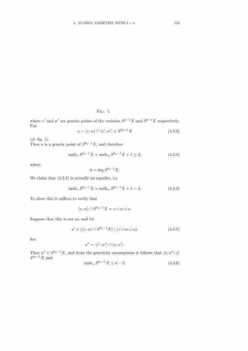
4. SCORZA VARIETIES WITH δ = 4 133
Fig. 1.
where v′ and w′ are generic points of the varieties Sa−1X and Sb−1X respectively.Put
u = 〈v, w〉 ∩ 〈v′, w′〉 ∈ Sk0−1X (4.3.2)
(cf. fig. 1).Then u is a generic point of Sk0−1X, and therefore
multv Sk0−1X + multw Sk0−1X + 1 ≤ d, (4.3.3)
whered = deg Sk0−1X.
We claim that (4.3.3) is actually an equality, i.e.
multv Sk0−1X + multw Sk0−1X + 1 = d. (4.3.4)
To show this it suffices to verify that
〈v, w〉 ∩ Sk0−1X = v ∪ w ∪ u.
Suppose that this is not so, and let
u′ ∈ (〈v, w〉 ∩ Sk0−1X) \ (v ∪ w ∪ u). (4.3.5)
Setu′′ = 〈v′, w′〉 ∩ 〈x, u′〉.
Then u′′ ∈ Sk0−1X, and from the genericity assumptions it follows that 〈x, u′′〉 6⊂Sk0−1X and
multx Sk0−1X ≤ d− 2. (4.3.6)
134 VI. SCORZA VARIETIES
Thus to prove (4.3.4) it suffices to show that (4.3.6) is impossible, i.e.
multx Sk0−1X = d− 1 (4.3.7)
(we recall that for all points v ∈ Sk0−1X we have
multv Sk0−1X < d (4.3.8)
since by Lemma 2.5 the variety Sk0−1X is not a cone).We begin with proving (4.3.4) in the case a = 1. We need to verify that for a
generic point v ∈ SXmultv Sk0−1X = d− 2. (4.3.9)
In fact, by (4.3.1) and (4.3.2), for a generic point w ∈ Sk0−1X we get a canonicallydefined point u ∈ 〈v, w〉 ∩ Sk0−1X (cf. fig.1). If multv Sk0−1X < d − 2, then fora general pair of points (v, w) ∈ SX × Sk0−1X the line 〈v, w〉 intersects Sk0−1Xtransversely in at least two more points u and u′ (cf. (4.3.5)). However, since thepoint u is chosen canonically, projecting Sk0−1X from the point v onto PN−1 weget a contradiction with the fact that Sk0−1X is an irreducible hypersurface andthe monodromy permutes the points u and u′.
Now (4.3.9) is proved for a generic point v ∈ SX. Actually from (4.3.2) and(4.3.8) it follows that (4.3.9) holds for an arbitrary point v ∈ SX \X. On the otherhand, for x ∈ X
d− 2 = multv Sk0−1X ≤ multx Sk0−1X ≤ d− 1.
Hence to prove (4.3.7) it suffices to show that
multx Sk0−1X > multv Sk0−1X.
Suppose that this is not so, and let x and y be generic points of X, u a genericpoint of Sk0−1X, and Π = 〈x, y, u〉 the plane spanned by x, y, and u. Then
Π ∩ Sk0−1X = 〈x, y〉 ∪ C,
where C ⊂ Π is a curve passing through u, and from (4.3.9) it follows that deg C =2. It is clear that for z ∈ 〈x, y〉 ∩ C
multz Sk0−1X = d− 1, (4.3.10)
and from (4.3.9) it follows that z ∈ X. Since x and y are generic points of X, from(4.3.10) and our assumption it follows that z 6= x, y, i.e., contrary to the trisecantlemma (cf. [39, 2.5; 34, Chapter IV, §3; 64, §7B], the chord 〈x, y〉 intersects X in atleast three points). The resulting contradiction proves (4.3.7) and hence (4.3.4) (weremark that (4.3.7) is a special case of (4.3.4) for a = 0).
Next we show that for generic points v ∈ SaX, w′ ∈ Sk0−a−1X = Sb−1X
multv Sk0−1X + multw′ Sk0−1X = d. (4.3.11)

4. SCORZA VARIETIES WITH δ = 4 135
Fig. 2.
In fact, it is clear that
d− 1 = multv Sk0−1X + multw Sk0−1X ≤ multv Sk0−1X + multw′ Sk0−1X ≤ d.
Suppose that〈v, w′〉 ∩ Sk0−1X 3 u, u 6= v, w′. (4.3.12)
Then for each point x ∈ Yv∩Yu (by Lemma 4.2, Yv∩Yu 6= ∅, dim Yv ∩ Yu ≥ (a−1)δ)and a generic point w ∈ 〈x,w′〉 we have
w ∈ SbX, 〈v, w〉 6⊂ Sk0−1X, 〈v, w〉 ∩ Sk0−1X 3 u = 〈v, w〉 ∩ 〈x, u〉(cf. fig. 2, where u ∈ 〈x, u′〉, v ∈ 〈x, v′〉, u′ ∈ Sk0−2X, v′ ∈ Sa−1X).
On the other hand,
〈v, w〉 ∩ Sk0−1X 3 u = 〈v, w〉 ∩ 〈v′, w′〉(cf. (4.3.2)). From the genericity assumptions it follows that u 6= u, i.e.
multv Sk0−1X + multw Sk0−1X ≤ d− 2
contrary to (4.3.4). Thus assumption (4.3.12) leads to a contradiction. Hence
〈v, w′〉 ∩ Sk0−1X = v ∪ w
which yields (4.3.11).From the system of equations (4.3.4) and (4.3.11) it follows that if v ∈ SaX,
v′ ∈ Sa−1X are generic points, 1 ≤ a ≤ k0 − 1, then
multv′ Sk0−1X = multv Sk0−1X + 1. (4.3.13)
Since for a generic point u ∈ Sk0−1X we have multu Sk0−1X = 1, successive appli-cation of (4.3.13) shows that for a generic point v ∈ SaX
multv Sk0−1X = k0 − a, 0 ≤ a ≤ k0 − 1. (4.3.14)
Combining (4.3.4) and (4.3.14), we get
d = (k0 − a) + (k0 − b) + 1 = k0 + 1. (4.3.15)
¤
136 VI. SCORZA VARIETIES
4.4. Lemma. Let Xn ⊂ PM(n,δ), δ = δ(X) > 0 be a Scorza variety. Supposethat n ≡ 0 (mod δ), and let u be a generic point of the hypersurface Sk0−1X.Then the projection πu : X 99K Pn with center at the subspace PN−n−1
u = 〈Yu〉 =Sk0−1Yu is a birational isomorphism. More precisely, let Hu = X ∩ Lu, whereLu = TSk0−1X,u. Then πu
∣∣X\Hu
is an isomorphism.
Proof. For a point x ∈ X we set Pu,x = 〈x,Pu〉. We observe that for x /∈ Hu wehave Pu,x 6⊂ Sk0−1X. In fact, if Pu,x ⊂ Sk0−1X, then
x ∈ X ∩ T (Pu, Sk0−1X) ⊂ Lu ∩X = Hu.
It is clear that the hypersurface Sk0−1X ∩Pu,x ⊂ Pu,x contains the linear subspacePu and the cone S(x, Sk0−2Yu) as its components. From Lemma 4.3 it follows that
1 + deg Sk0−2Yu = deg(Sk0−1X ∩ Pu,x
) ≤ deg Sk0−1X = k0 + 1. (4.4.1)
On the other hand, in view of Theorem 1.4, Lemma 4.3 can also be applied to theScorza variety Yu, dim Yu = (k0 − 1)δ, k0(Yu) = k0 − 1 ≥ 2 (the case k0 = 2 wasalready considered in Chapter IV), so that
deg(Sk0−2Yu
)= k0. (4.4.2)
From (4.4.2) it follows that the inequality (4.4.1) is actually an equality, and there-fore
Sk0−1X ∩ Pu,x = Pu ∩ S(x, Sk0−2Yu). (4.4.3)
SinceS(y, Sk0−2Yu) ⊂ Sk0−1X ∩ Pu,x,
for each point y ∈ (Pu,x \ Pu) ∩X, from (4.4.3) it follows that
X ∩ Pu,x = (X ∩ Pu) ∪ x = Yu ∪ x, (4.4.4)
i.e. π−1u
(πu(x)
)= x, which implies our claim. ¤
We turn to a more detailed description of the hyperplane section Hu = Lu ·X(we recall that from Corollary 1.15 a) in Chapter I it follows that if δ > 1, thenHu = Lu ∩X is a reduced variety). From Lemma 2.2 it follows that for a genericpoint z ∈ SX the intersection Yz ∩ Yu consists of a single point y. Furthermore,
(Hu · Yz)X = (Lu · Yz)PN = (TYz,y · Yz)Pz
is a cone with vertex y over a nonsingular (δ − 2)-dimensional quadric.Let y ∈ Yu be a generic point, and let Cy =
⋃z(Hu · Yz)X , where z runs through
the set of general points of the cone S(y, X). Then Cy is a cone with vertex y whosebase is an irreducible variety By such that
2 dim By − 2(δ − 2) = n− δ
4. SCORZA VARIETIES WITH δ = 4 137
(here n−δ = [(n+1)− (δ+1)] is the dimension of the family of quadrics Yz passingthrough y), i.e.
dim By =n + δ − 4
2, dim Cy =
n + δ − 22
.
Varying y in the set of general points of Yu, we obtain an irreducible variety Cu =⋃yCy ⊂ Hu. Furthermore, if x1, x2 is a general pair of points of Cu and z is a general
point of 〈x1, x2〉, then Yz ∩ Lu is the cone over a nonsingular (δ − 2)-dimensionalquadric with vertex at the (unique) intersection point y ∈ Yz ∩ Yu. In other words,Bu
x1∩Bu
x2= y, where
Buxi
=y ∈ Yu
⟨xi, y 〉 ⊂ X
, i = 1, 2. (4.4.5)
From this it follows thatdim Bu
xi=
dim Yu
2, (4.4.6)
i.e. a generic point x ∈ Cu is contained in a(
n−δ2
)-dimensional family of lines of
the above type. Hence
dim Cu = (n− δ) +n + δ − 2
2− n− δ
2= n− 1,
i.e. Cu consists of components of Hu. But from Corollary 1.15 b) in Chapter I itfollows that for δ > 2 the hyperplane section Hu is irreducible. Taking into accountthat each line in X passing through y is contained in TX,y, we can sum up thepreceding discussion in the following lemma.
4.5. Lemma. In the conditions of Lemma 4.4 suppose in addition that δ > 2.Then Hu = X ∩ Lu = X ∩ T (Yu, X) = Cu coincides with the closure of a union ofall lines lying in X and intersecting Yu.
4.6. We return to the case δ = 4, n ≡ 0 (mod 4). Let x be a generic point ofHu. Put Dx =
⋃zYz, where z runs through the set of general points of the cone
S(x, Yu). Since for a generic point y ∈ Yu and a generic point z ∈ 〈x, y〉
Yz ∩ Lu ⊃ (TYz,y ∩ Yz)
andYz ∩ Lu 3 x, x /∈ TYz,y ∩ Yz,
we see that Yz ⊂ Lu and therefore
Yu ⊂ Dx ⊂ Hu, (4.6.1)
where from the definition of Dx and the proof of Lemma 4.5 it follows that bothinclusions are strict. Since
dim Dx = (n− 4) + 4− dim Yz ∩ Yu = dim Hu − (dimYz ∩ Yu − 1),
138 VI. SCORZA VARIETIES
we conclude that dim Yz ∩ Yu = 2 and Dx is a divisor on Hu (arguing as in theproof of Proposition 3.2 in Chapter IV, it is easy to show that Yz ∩ Yu = P2).
If x′ ∈ Dx is another generic point, then Dx′ = Dx. In fact, let a ∈ Dx bea generic point, and let z′ be a generic point of the line 〈a, x′〉. Then Yz′ is anonsingular four-dimensional quadric,
x′ ∈ Yz′ , Yz′ ∩ Yu 6= ∅, a ∈ Yz′ ⊂ Dx. (4.6.2)
Thus, varying x ∈ Hu, we obtain a one-dimensional family of divisors Dx ⊂ Hu.From the proof of Lemma 4.5 it follows that the base of this family is an imageof the line 〈x, x′〉, where x, x′ is a general pair of points of Hu, so that the familyDx is rational.
If x0, . . . xi, 0 ≤ i ≤ k0 − 1 is a general collection of points of Dx and v is ageneric point of the i-dimensional linear subspace 〈x0, . . . , xi〉, then
Yv ⊂ Dx. (4.6.3)
In fact, from (4.6.2) it follows that (4.6.3) holds for i = 1. On the other hand, theproof of Theorem 1.8 of Chapter V shows that if a is a generic point of Dx, w is ageneric point of Si−1Dx, and v is a generic point of 〈x, w〉, then Yv =
⋃zYz, where
z runs through the set of generic points of the cone S(a, Yw). Thus (4.6.3) can beeasily proved by induction on i.
In particular, if u′ is a generic point of Sk0−1Dx, then Yu′ ⊂ Dx ⊂ Hu′ , so that
Dx ⊂⋂
u′∈Sk0−1Dx
Hu′ . (4.6.4)
From (4.6.3) and formulas (1.5.4) and (1.5.8) in Chapter V it follows that
dim Sk0−1Dx = dim Sk0−2Dx + [(n− 1)− (n− 4)]
= dim Sk0−3Dx + [(n− 1)− (n− 4)] + [(n− 1)− (n− 8)]
= · · · = (4k0 − 2) + 3 + 7 + · · ·+ [3 + 4(k0 − 2)] = 2k20 + k0 − 1.
By Theorem 1.4, the hyperplane Lu′ is tangent to Sk0−1X along the linear subspace
Pu′ = Sk0−1Yu′ , dimPu′ = N − n− 1 = 2k20 − k0 − 1.
Hence, varying u′ ∈ Sk0−1Dx, we obtain a [(2k20 + k0 − 1)− (2k2
0 − k0 − 1)] = 2k0-dimensional family of hyperplane sections Hu′ of the variety X passing throughthe (n − 2)-dimensional subvariety Dx ⊂ Hu. It is clear that this family cuts a(2k0 − 1)-dimensional family of hyperplane sections of the variety Hu containingDx as an irreducible component.
By Barth’s theorem (cf. [6; 33]), H1(X,OX) = 0, and the exact sequence
0 → H0(X,OX) → H0(X,OX(1)) → H0(Hu,OHu(1)) → H1(X,OX(1))
4. SCORZA VARIETIES WITH δ = 4 139
shows that the variety Hu ⊂ PN−1 is linearly normal (the Scorza variety X ⊂ PN
is linearly normal by definition).Thus we obtain two linear systems I = |Dx| and II = |(Hu′ ·Hu) −Dx| on the
variety Hu whose fundamental subset coincides with Yu. We have already shownthat
dim I ≥ 1, dim II ≥ 2k0 − 1. (4.6.5)
Since Hu is linearly normal,
dim H0(Hu,OHu(1− Yu)) = dimπu(Hu) = n− 1 = 4k0 − 1 (4.6.6)
(here |[OHu(1 − Yu)]| is the linear system of hyperplane sections of Hu passingthrough Yu). From (4.6.5) and (4.6.6) it follows that
dim I = 1, dim II = 2k0 − 1.
Furthermore, the linear system I maps Hu onto P1, the linear system II maps Hu
onto P2k0−1, and the projection πu with center in Pu defined by the linear system|[O(1 − Yu)]| maps Hu onto P1 × P2k0−1. In the proof of Lemma 4.5 we actuallyshowed that the fibers of πu
∣∣Hu
are cones
π−1u
(πu(x)
)= Pu,x ∩X = Cu
x
with vertex x ∈ Hu \ Yu and base Bux ,
dim Bux =
dim Yu
2= 2k0 − 2, dim Cu
x = 2k0 − 1.
Furthermore, arguing as in the proof of Proposition 3.2 in Chapter IV or using in-duction on n, it is easy to verify that Bu
x = Cux∩Yu is a linear subspace and therefore
the fibers of the projection πu
∣∣Hu
are (2k0 − 1)-dimensional linear subspaces.Summing up the above discussion, we get the following result.
4.7. Lemma. In the conditions of Lemma 4.5 suppose in addition that δ =4. Then πu(Hu) ⊂ πu(Lu) ⊂ πu(PN ) = P1 × Pn
2−1 ⊂ Pn−1 ⊂ Pn (the Segreembedding), and a generic fiber of the map πu
∣∣Hu
99K P1×Pn2−1 is a linear subspace
of Pn2−1.
4.8. Consider the map
σu = π−1u : Pn 99K P
n(n+6)8 , σu(Pn) = X.
From Lemma 4.7 it follows that σu is defined by a linear system of hypersurfacesin Pn passing through P1 × Pn
2−1 ⊂ Pn−1 ⊂ Pn. Since P1 × Pn2−1 is defined in
Pn by((n + 1) +
(n22
))= n2+6n+8
8 = N + 1 quadratic equations, from the linearnormality of X it follows that σu is defined by the linear system of quadrics in Pn
passing through P1 × Pn2−1.
Theorem 4.1 in the case n ≡ 0 (mod 4) now follows from the characterization ofGrassmannians (cf. [81] and also § 3 of Chapter III).
140 VI. SCORZA VARIETIES
4.9. Lemma. Let Xn ⊂ PM(n,4), δ(X) = 4 be a Scorza variety. Then n 6≡ 1(mod 4).
Proof. Suppose the converse, and let u be a generic point of PN = Sk0X,
N = M(n, 4) = f(k0) =n2 + 6n + 1
8.
By Theorem 1.4, Yu = X ∩ Pu is a Scorza variety of dimension 4k0 = n − 1in the linear subspace Pu = 〈Yu〉 ⊂ PN , dimPu = n2+4n−5
8 < N − 1. Hencefor a general hyperplane L ⊃ Pu we have L ·X > Yu which contradicts the Barth-Larsen theorem according to which H2n−2(X,Z) and Pic X are infinite cyclic groupsgenerated by the classes of hyperplane section (cf. [54; 65]). This contradictionproves Lemma 4.9. ¤
4.10. We turn to the case n ≡ 2 (mod 4). Let
Xn ⊂ PN , n ≡ 2 (mod 4), N =n(n + 6)
8(4.10.1)
be a Scorza variety. According to Theorem 1.4, if u ∈ PN = Sk0X is a genericpoint, then Yu = X ∩ Pu is a Scorza variety of dimension 4k0 = n− 2 in the linearsubspace Pu = 〈Yu〉 ⊂ PN ,
dimPu =(n− 2)(n− 4)
8= N − n
2 − 1. (4.10.2)
Let u′ ∈ PN be another generic point. Then
Yu′ = X ∩ Pu′ , Yu ∩ Yu′ = Yu ∩ Pu′ , (4.10.3)
and since dim Yu +dimPu′ = (n− 2)+ (N − n2 − 1) > N, we see that Yu ∩Yu′ 6= ∅.
From Theorem 1.4 it immediately follows that
δ(Yu ∩ Yu′) = δ(Yu) = δ(X) = 4. (4.10.4)
Furthermore, for a general pair of points u, u′ ∈ PN we have
dim Yu ∩ Yu′ = n− 4. (4.10.5)
In fact, if we had
dim Yu ∩ Yu′ = dim Yu ∩ Pu′ = n− 3 = dim Yu − 1,
then Yu ∩ Yu′ would coincide with a hyperplane section of Yu which contradicts(4.10.4).
From Theorem 1.4 and the already proven part of Theorem 4.1 it follows that
Yu = G(2k0 + 1, 1). (4.10.6)
4. SCORZA VARIETIES WITH δ = 4 141
From (4.10.3), (4.10.4), (4.10.5), and (4.10.6) it is easy to deduce that
Y = Yu ∩ Yu′ = G(2k0, 1) (4.10.7)
is the Schubert cycle in Yu = G(2k0 +1, 1) parametrizing the lines contained in thehyperplane P2k0 ⊂ P2k0+1. It also easily follows that
Pu ∩ Pu′ = 〈Y 〉 = PY , dimPY = (n−4)(n+2)8 = N − n− 1.
PutL = 〈Pu,Pu′〉, dim L = 2(N − n
2 − 1)− (N − n− 1) = N − 1.
From the definition it follows that the hyperplane L is tangent to X along thesubvariety Y , i.e. T (Y,X) ⊂ L. Denote by H the hyperplane section X ∩L and byπY : X 99K Pn the projection with center at PY .
Varying a generic point u′′ ∈ PN , we obtain an (N − dimPu′′) = (n2 − 1)-
dimensional rational family of subvarieties Yu′′ ⊂ X. Furthermore, if
Yu ∩ Yu′′ = Yu ∩ Yu′ = Y, (4.10.8)
then〈Pu,Pu′′〉 = 〈Pu,Pu′′〉 = L.
In this caseY n−2
u′′ ⊂ Hn−1, (4.10.9)
and it is clear that a generic point of H is contained only in a finite number ofsubvarieties Yu′′ satisfying condition (4.10.8). Since on the Grassmannian G(2k0 +1, 1) there is a dimP(2k0+1)∗ = (2k0 +1) = n
2 -dimensional family of GrassmanniansG(2k0 +1), from (4.10.7) it follows that a general variety Y = Yu ∩Yu′ = G(2k0, 1)is contained in a one-dimensional rational family of Yu′′ and
H =⋃
Yu′′∩Yu=Y
Yu′′ (4.10.10)
(cf. (4.10.9)). A word-for-word repetition of the arguments used in the proof ofLemma 4.7 (with the linear system |Dx|, Yu ⊂ Dx ⊂ Hu replaced by the linearsystem |Yu′′ |, Y ⊂ Yu′′ ⊂ H) shows that
πY
∣∣H
: H 99K P1 × Pn2−1 ⊂ Pn−1 ⊂ Pn = πY (X) (4.10.11)
is a rational fiber bundle with fiber Pn2−1.
We claim that for a generic point x ∈ X \H
PY,x ∩X = Y ∪ x, (4.10.12)
where PY,x = 〈PY , x〉. Suppose that this is not so, and let
y ∈ PY,x ∩X, y ∈ Y, y 6= x. (4.10.13)
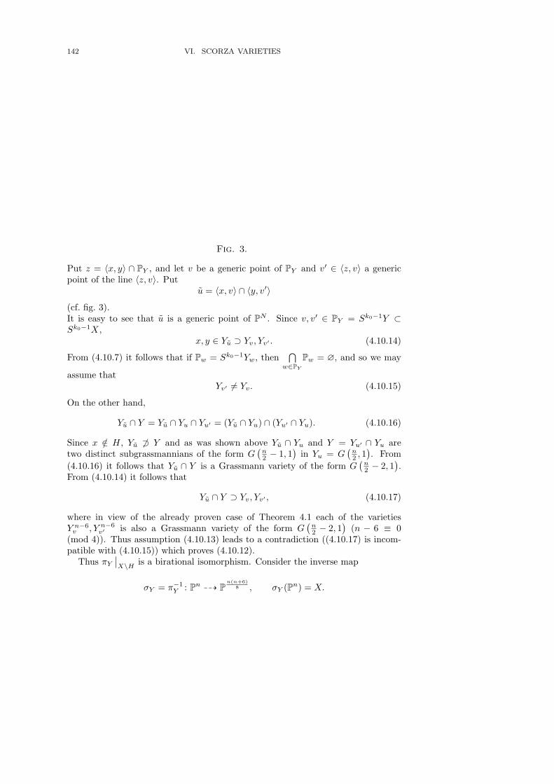
142 VI. SCORZA VARIETIES
Fig. 3.
Put z = 〈x, y〉 ∩ PY , and let v be a generic point of PY and v′ ∈ 〈z, v〉 a genericpoint of the line 〈z, v〉. Put
u = 〈x, v〉 ∩ 〈y, v′〉(cf. fig. 3).It is easy to see that u is a generic point of PN . Since v, v′ ∈ PY = Sk0−1Y ⊂Sk0−1X,
x, y ∈ Yu ⊃ Yv, Yv′ . (4.10.14)
From (4.10.7) it follows that if Pw = Sk0−1Yw, then⋂
w∈PY
Pw = ∅, and so we may
assume thatYv′ 6= Yv. (4.10.15)
On the other hand,
Yu ∩ Y = Yu ∩ Yu ∩ Yu′ = (Yu ∩ Yu) ∩ (Yu′ ∩ Yu). (4.10.16)
Since x /∈ H, Yu 6⊃ Y and as was shown above Yu ∩ Yu and Y = Yu′ ∩ Yu aretwo distinct subgrassmannians of the form G
(n2 − 1, 1
)in Yu = G
(n2 , 1
). From
(4.10.16) it follows that Yu ∩ Y is a Grassmann variety of the form G(
n2 − 2, 1
).
From (4.10.14) it follows that
Yu ∩ Y ⊃ Yv, Yv′ , (4.10.17)
where in view of the already proven case of Theorem 4.1 each of the varietiesY n−6
v , Y n−6v′ is also a Grassmann variety of the form G
(n2 − 2, 1
)(n − 6 ≡ 0
(mod 4)). Thus assumption (4.10.13) leads to a contradiction ((4.10.17) is incom-patible with (4.10.15)) which proves (4.10.12).
Thus πY
∣∣X\H is a birational isomorphism. Consider the inverse map
σY = π−1Y : Pn 99K P
n(n+6)8 , σY (Pn) = X.
4. SCORZA VARIETIES WITH δ = 4 143
From the already proven case of Theorem 4.1 it follows that for a generic pointu ∈ PN
πY (Yu) = Pu ⊂ Pn, dimPu = n− 2,
and if Pn−1 = 〈πY (H)〉, then
Pu ∩ Pn−1 = 〈P1 × Pn2−2〉, P1 × Pn
2−2 = πY (Yu ∩H) ⊂ πY (H) = P1 × Pn2−1.
Suppose that σY is defined by n2+6n+88 forms G0, . . . , Gn(n+6)
8, deg Gi = d, i =
0, . . . , n(n+6)8 . As it was shown in 4.8, after canceling the greatest common divisor
Gi
∣∣Pu
become quadratic forms. Varying generic point u ∈ PN , we see that d = 2.
Since P1 × Pn2−1 is defined in Pn by (n + 1) +
(n22
)= n2+6n+8
8 = N + 1 quadraticequations and
Gi
∣∣P1×Pn
2 −1= 0, i = 0, . . . ,n(n + 6)
8,
from this it follows that σY is defined by the linear system of quadrics in Pn passingthrough P1 × Pn
2−1.Theorem 4.1 in the case n ≡ 2 (mod 4) now follows from the characterization of
Grassmann varieties (cf. [81] and § 3 of Chapter III).It remains to consider the case n ≡ 3 (mod 4).
4.11. Lemma. Let Xn ⊂ PM(n,4), δ(X) = 4 be a Scorza variety. Then n 6≡ 3(mod 4).
Proof. Suppose that the lemma does not hold, and let u be a generic point ofPN = Sk0X,
k0 =n− 3
4, N = M(n, 4) = f(k0) =
n2 + 6n− 38
,
and u′ a generic point of S(Yu, Sk0−1X). Then u′ is a generic point of PN , and (byTheorem 1.4) Yu and Yu′ are Scorza varieties of dimension n− 3. From the alreadyproven case of of Theorem 4.1 it follows that Yu and Yu′ are projectively isomorphicto the Grassmann variety of lines in P
n−12 . Denote by Y the intersection Yu ∩ Yu′ .
It is clear thatdim Y ≥ n− 6, δ(Y ) = 4, (4.11.1)
and if z ∈ SY \ Y , then Yz ⊂ Y . Geometrically this means that if the subvarietyY ⊂ G
(n−1
2 , 1)
contains a pair of points α1, α2 corresponding to non-coplanarlines l1, l2 ⊂ Pn−1
2 , then for each line l ⊂ 〈l1, l2〉 the subvariety Y contains a pointα ∈ G
(n−1
2 , 1)
corresponding to this line. From this it follows that
Y = G(m, 1), (4.11.2)
where Pm ⊂ Pn−1
2 is a linear subspace. It is clear that the only subvariety Y ⊂G
(n−1
2 , 1)
satisfying conditions (4.11.1) and (4.11.2) is the Grassmann subvarietyY = G
(n−3
2 , 1).
144 VI. SCORZA VARIETIES
We observe that if u′ ∈ 〈x, v〉, where x ∈ Yu, v ∈ Sk0−1X are generic points andz is a generic point of Y 1
v = p1,k0−30
((ϕ1,k0−3)−1(v)
), then z is a generic point of
SX ,
Yz → Yv → Yu′ =
G(3, 1) → G
(n− 5
2, 1
)→ G
(n− 1
2, 1
),
Y → Yu′ =
G
(n− 3
2, 1
)→ G
(n− 1
2, 1
),
and therefore for a generic pair of points u ∈ Sk0−1X, z ∈ SX
Yu ∩ Yz = G(2, 1) = P2. (4.11.3)
But from (4.11.3) it follows that
S(Yu, X) = SX, dim ϕ−1Y (z) = 2
while we already know that for a generic point z ∈ SX
dim ϕ−1Yu
(z) = dim Yu + n + 1− dim SX = 1.
¤Now all the four cases in Theorem 4.1 are verified, and the proof of the theorem
is complete. ¤4.12. Remark. For δ = 4, n ≤ 7 we have k0 = 1, and each variety Xn ⊂ P2n−3
is extremal. In other words,
M(7, 4) = m(7, 4) = 11, M(6, 4) = m(6, 4) = 9,
M(5, 4) = m(5, 4) = 7, M(4, 4) = m(4, 4) = 5.
4.13. Corollary. Let Xn ⊂ Pr be a nonsingular variety, r ≤ 2n − 3. Then
h0(X,OX(1)
) ≤[
(n+3)2
8
]with equality holding if and only if r = 2n− 3 and either
n ≤ 7 or n ≡ 0 (mod 2) and X → Pr is the embedding of the Grassmann varietyG
(n2 + 1, 1
) ' X defined by a collection (Q0 : · · · : Q2n−3) of 2n − 2 linear formsof the Plucker coordinates.
5. END OF CLASSIFICATION OF SCORZA VARIETIES 145
5. End of classification of Scorza varieties
It remains to classify Scorza varieties with δ = 8.
5.1. Lemma. Let Xn ⊂ PM(n,8), δ(X) = 8 be a Scorza variety. Then k0 =[n8
]= 2.
Proof. Suppose that k0 ≥ 3, and let v be a generic point of S3X. From The-orem 1.4 it follows that Y 24
v is a Scorza variety with δ(Y ) = 8. Hence to proveLemma 5.1 it suffices to verify that a 24-dimensional variety with δ = 8 does notexist.
In fact, if X were such a variety, then we would have an ascending chain of secantvarieties
X24 ⊂ (SX)41 ⊂ (S2X)50 ⊂ S3X = P51.
Let u be a generic point of S2X. Put
Lu = TS2X,u, Hu = (Lu ·X)P51 = Lu ∩X.
Let x ∈ Hu be a generic point. In the proof of Lemma 4.5 it was shown thatBu
x = y ∈ Yu
∣∣ 〈x, y〉 ⊂ X is a dim Yu
2 =8-dimensional subvariety of Yu (cf. (4.4.5),(4.4.6)). As in 4.6, we see that Bu
x = SBux , and therefore Bu
x is a linear subspace(cf. the proof of Lemma 3.6 in Chapter IV). Hence in order to prove Lemma 5.1it suffices to verify that the Severi variety Yu = E16 ⊂ P24 does not contain eight-dimensional linear subspaces.
We claim that E16 actually does not contain even six-dimensional linear sub-spaces (we recall that for z ∈ SE \ E we have π−1
z
(πz(x)
)= P5 for each point
x ∈ Hz = Lz ∩X, x /∈ Yz, so that E contains five-dimensional linear subspaces; cf.also [13]). In fact, if E16 ⊃ P6 3 x, then
TE∩x ∩ E ⊃ P6. (5.1.1)
In view of the results of §2 of Chapter III (cf. also Chapter IV, 4.2 c), 4.3), TE,x ∩E is a cone with vertex x and base S10, where S10 ⊂ P15 is the spinor varietycorresponding to the orbit of highest weight vector of the spinor representation ofthe group Spin10. Hence from (5.1.1) it follows that S10 ⊃ P5. But for an arbitrarypoint y ∈ P5 ⊂ S10
TS,y ∩ S ⊃ P5 (5.1.2)
is a cone with vertex y and base G(4, 1) ⊂ P9 (cf. §2 in Chapter III). Hence from(5.1.2) it follows that G(4, 1) ⊃ P4. But for an arbitrary point α ∈ P4 ⊂ G(4, 1)
TG(4,1),α ∩G(4, 1) ⊃ P4 (5.1.3)
is a cone with vertex α and base P1 × P2 ⊂ P5 (cf. again §2 of Chapter III). Hence(5.1.3) would imply that P1 × P2 ⊃ P3 which is clearly impossible.
This completes the proof of Lemma 5.1. ¤From Lemma 5.1 it follows that the dimension n of a Scorza variety Xn with
δ(X) = 8 satisfies the inequalities
16 ≤ n ≤ 23.
146 VI. SCORZA VARIETIES
5.2. Lemma. Let Xn be a Scorza variety such that δ(X) = 8 and k0(X) = 2.Then n = 16 and X = E is a Severi variety.
Proof. Suppose that 17 ≤ n ≤ 23. Then N = M(n, 8) = f(2) = 26 + 3ε,ε = n mod 8, and for a generic point u ∈ S2X = PN
Y 16
u ⊂ P26
=E16 ⊂ P26
is a sixteen-dimensional Severi variety (cf. Theorem 1.4). Let u′ be a generic pointof S(Yu, SX). Then u′ is a generic point of PN , and Yu′ is a sixteen-dimensionalSeveri variety.
Put Y = Yu ∩ Yu′ . It is clear that Y is a nonsingular variety,
9 = 32− 23 ≤ dim Y ≤ 15, (5.2.1)
and if z ∈ SY \ Y , then Yz ⊂ Y (cf. the proof of Lemma 4.11). From (5.2.1) andCorollary 2.11 in Chapter II it follows that
SY = Pr, r = 2dim Y − 7 ≥ 11,
and thereforeSE ⊃ P11. (5.2.2)
But according to the results of §2 of Chapter III and Remark 2.5 in Chapter IV(SE)∗ ' E and each hyperplane TSE,z (z ∈ SE \ E) is tangent to SE along thelinear subspace P9
z = 〈Yz〉. Since for z ∈ P11 \ E
TSX,z ⊃ P11, (5.2.3)
from (5.2.2) and (5.2.3) it follows that P11 ⊂ E. But in the proof of Lemma 5.1 weverified that the variety E does not contain even six-dimensional linear subspaces.The resulting contradiction proves Lemma 5.2 (the non-existence of Scorza varietiesXn with 17 ≤ n ≤ 19 can be more easily deduced from the Barth-Larsen theorem[54], but we prefered to give a more uniform proof). ¤
Combining the assertions of Lemmas 5.1 and 5.2 and Theorem 4.7 in Chapter IVwe obtain the following result.
5.3. Theorem. Let Xn ⊂ PN , n ≥ 16 be a nonsingular nondegenerate variety.
Suppose that sX < 2n− 6. Then N ≤ n(n+10)+ε(6−ε)16 , ε = n mod 4. Furthermore,
equality holds if and only if X = E ⊂ P26 is a sixteen-dimensional Severi varietycorresponding to the orbit of highest weight vector of the simplest representation
of the group E6. In other words, M(16, 8) = 26 and M(n, 8) < n(n+10)+ε(6−ε)16 for
n > 16.
5.4. Remark. For δ = 8, 8 ≤ n ≤ 15 we have k0 = 1 and each variety Xn ⊂P2n−7 is extremal. In other words,
M(n, 8) = m(n, 8) = 2n− 7, 8 ≤ n ≤ 15.
5. END OF CLASSIFICATION OF SCORZA VARIETIES 147
5.5. Corollary. Let Xn ⊂ Pr be a nonsingular variety, r ≤ 2n − 7. Then
h0(X,OX(1)) ≤[
(n+5)2
16
]with equality holding if and only if r = 2n − 7 and
either n ≤ 14 or n = 16 and X ⊂ P25 is an isomorphic projection of the sixteen-dimensional Severi variety E16 ⊂ P26.
Combining Theorems 2.1, 3.1, 4.1, and 5.3 and taking into account properties ofthe function f depicted on fig. 3 in Chapter V, we obtain the following
5.6. Classification theorem. Let Xn ⊂ PN be a nonsingular nondegener-
ate variety over an algebraically closed field K. Then N ≤ n(n+δ+2)+ε(δ−ε−2)2δ ≤[
(n+ δ2+1)2
2δ
]− 1, where δ = 2n + 1 − s, s = dim SX, ε = δ
nδ
= n mod δ. If
charK = 0, then N = n(n+δ+2)+ε(δ−ε−2)2δ in the following cases:
(0) n < 2δ, ε = n− δ, s = N = 2n + 1− δ;(i) δ = 1, N = n(n+3)
2 , X = v2(Pn) is the Veronese variety;
(ii) δ = 2, N = n(n+4)−nmod24 , X = P[n
2 ] × P[n+12 ] is the Segre variety;
(iii) δ = 4, n ≡ 0 (mod 2), N = n(n+6)8 , X = G
(n2 + 1, 1
)is the Grassmann
variety;(iv) δ = 8, n = 16, N = 26, X = E is the sixteen-dimensional Severi variety.
The varieties (i)–(iv) are Scorza varieties, and for them N =[
(n+ δ2+1)2
2δ
]− 1.
The Scorza variety Xn corresponds to the orbit of highest weight vector of anirreducible representation of a semisimple group G in a vector space V with highestweight Λ, where
(i) G = SLn+1, Λ = 2ϕ1;(ii) G = SL[n+2
2 ] × SL[n+32 ], Λ = ϕ1 ⊕ ϕ1;
(iii) G = SLn2 +2, Λ = ϕ2;
(iv) G = E6, Λ = ϕ1
(here ϕi is the i-th fundamental weight).The Scorza variety Xn is the image of Pn under the rational map σ : Pn 99K PN
defined by the linear system of quadrics passing through the subvariety A ⊂ Pn−1 ⊂Pn, where
(i) A = ∅;(ii) A = P[
n−22 ] ∐P[n−1
2 ];(iii) A = P1 × Pn
2−1;(iv) A = S10.
In other words, the Scorza variety Xn is obtained from the Veronese variety
v2(Pn) ⊂ Pn(n+3)
2 by projecting from the linear span 〈v2(A)〉 of the image of thevariety A ⊂ Pn under the Veronese map v2.
5.7. Remark. As in Remark 4.3 in Chapter IV, it is not hard to verify that foran arbitrary point x of the Scorza variety Xn ⊂ PN the variety TX,x ∩X is a conewith vertex x and base A. Under the map π = (σ
∣∣X
)−1 each of the cones TX,x ∩X
is mapped onto its base. The map π is an isomorphism outside of σ(Pn−1) and
σ(Pn−1) =⋃
y∈Sing σ(Pn−1)
TX,y ∩X, π : σ(Pn−1) → A.
148 VI. SCORZA VARIETIES
5.8. Remark. As in Remark 4.6 in Chapter IV, it is not hard to verify thatthe linear system of quadrics cut in a general linear subspace Pn−1 ⊂ TX,x bythe linear system of quadrics passing through the Scorza variety X and defining arational map Pn−1 99K Y x ⊂ PM(n−δ,δ) (where Y x ⊂ X∗ is naturally isomorphicto Sing
(σ(Pn−1)
)) is the second fundamental form in the sense of [29] and the
subvariety A ⊂ Pn−1 is the fundamental subset of this form.
Combining Corollaries 2.9, 3.5, 4.13, and 5.5 with Theorem 2.10 of Chapter Vwe obtain the following.
5.9. Theorem. Let Xn ⊂ Pr be a nonsingular variety over an algebraically
closed field K. Then h0(X,OX(1)) ≤[
(4n−r+3)2
8(2n−r+1)
]. If in addition charK = 0 and
r ≥ 3n2 + 1, then equality holds if and only if X is an isomorphic projection of
a Scorza variety X to a projective space Ps, s = dim SX, so that in particularr = 2n, 2n − 1, 2n − 3 or 2n − 7 (if r < 3n
2 + 1, then from Corollary 2.11 in
Chapter II it follows that h0(X,OX(1)
)= r + 1).
5.10. Remark. It is worthwhile to observe that in the most important casewhen n ≡ 0 (mod δ) classification of Scorza varieties over an algebraically closedfield K, charK = 0 is parallel to classification of Jordan matrix algebras due toAlbert (cf. [10; 44, Chapter V ]). More precisely, PN = P
(Jn
δ +1
)where Jn
δ +1 is theJordan algebra of Hermitean matrices of order n
δ +1 over a composition algebra A,dimK Jn
δ +1 = (n+δ)(n+2)2 (we recall that for A = A0, A1, A2
nδ ≥ 2 is an arbitrary
integer and Jnδ +1 is a special Jordan algebra and for A = A3 we have n
δ = 2and J3 is an exceptional Jordan algebra; cf. Theorem 4.8 in Chapter III) and Xcorresponds to the cone
A ∈ Jn
δ +1
∣∣ rk A ≤ 1. More generally, the variety SkX,
0 ≤ k ≤ k0 = nδ corresponds to the cone
A ∈ Jn
δ +1
∣∣ rk A ≤ k + 1.
Arguing as in Theorem 4.9 of Chapter IV, we can restate Remark 5.10 as follows.
5.11. Theorem. A nonsingular nondegenerate variety Xn ⊂ PN , n ≡ 0(mod δ), N = f
(nδ
), δ = δ(X) over an algebraically closed field K, charK = 0
is a Scorza variety if and only if X is the ‘Veronese variety’ of dimension nδ ≥ 2
over the composition algebra A, dimK A = δ, i.e. X is the image of the ‘projectivespace’ Pn
δ (A) =(A
nδ +1 \ 0
)/A∗ (where A∗ is the subset of invertible elements of
the algebra A) under the map (x0 : · · · : xnδ)
v299K (· · · : xlxm : . . . ), 0 ≤ l ≤ m ≤ nδ
(for δ = 8 we have n = 16 since, due to the lack of associativity, for larger n thevariety v2
(Pn
8 (A3))
is no longer defined by vanishing of the minors of order two of a
Hermitean(
n8 + 1
)× (n8 + 1
)-matrix; this corresponds to J3 being the only Jordan
matrix algebra over A3).
References
1. A. Alzati and G. Ottaviani, A linear bound on the t-normality of codimension two subvarietiesof Pn, J. reine angew. Math. 409 (1990), 35–40.
2. E. M. Andreev, E. B. Vinberg, and A. G. Elashvili, Orbits of maximal dimension of semisimpleLie groups, Funk. Anal. i ego Prilozh. 1 no. 4 (1967), 3–7 (Russian); English transl. in: Func.Anal. Appl.
3. L. Bai, C. Musili, and C. Seshadri, Cohomology of line bundles on G/B, Ann. Sci. ENS 7(1974), 89–138.
4. E. Ballico and L. Chiantini, On smooth subcanonical varieties of codimension 2 in Pn, n ≥ 4,Ann. Mat. Pura ed Appl. 135 (1983), 99-117.
5. W. Barth, Fortsetzung meromorpher Funktionen in Tori und komplex-projektiven Raumen,Invent. Math. 5 (1968), 42–62.
6. , Transplanting cohomology classes in complex projective space, Amer. J. Math. 92(1970), 951-967.
7. A. Borel, Linear algebraic groups, W. A. Benjamin, New York - Amsterdam, 1969.
8. A. Borel and F. Hirzebruch, Homogeneous spaces and characteristic classes II, Amer. J. Math.81 (1959), 315–382.
9. N. Bourbaki, Groupes et algebres de Lie, Hermann, Paris.
10. H. Braun and M. Koecher, Jordan-Algebren, Springer-Verlag, Berlin - Heidelberg - New York,1966.
11. W. Burau, Mehrdimensionale Projektive und hohere Geometrie, Deutscher Verl. der Wis-senschaften, Berlin, 1961.
12. E. Cartan, Sur la structure des groupes des transformations finis et continus, Oeuvres com-plete. Partie I, vol. 1, Paris, 1952.
13. C. Chevalley, Sur le groupe exceptionel E6 et sur une variete algebrique liee a l’etude de cegroupe., C. R. Acad. Sci. Paris 232 (1951), 1991–1993; 2168–2170.
14. M. Dale, On the secant variety of an algebraic surface, Preprint no. bf33, Univ. Bergen,Bergen, Norway, 1984.
15. , Severi’s theorem on the Veronese surface, J. London Math. Soc. (2) 32, 419–425.
16. P. Deligne and N. Katz, Groupes de monodromie en geometrie algebrique (SGA7), LectureNotes in Math. 340, Springer-Verlag, Berlin - Heidelberg - New York, 1973.
17. J. Dieudonne and J. Carrell, Invariant theory, old and new, Academic Press, New York -London, 1971.
18. L. Ein, The ramification divisors for branched coverings of Pnk , Math. Ann. 261 (1982),
483-485.
19. , Vanishing theorems for varieties of low codimension, in: Algebraic Geometry, Sun-dance 1986. Proceedings (A. Holme and R. Speiser, eds.), Lecture Notes in Math. 1311,Springer-Verlag, Berlin - Heidelberg - New York.
20. A. G. Elashvili, Canonical form and stationary subalgebras of generic points for simple linearLie groups, Funk. Anal. i ego Prilozh. 6 no. 1 (1972), 51–62 (Russian); in: Func. Anal. Appl.
21. G. Faltings, Verschwindungsstze und Untermannigfaltigkeiten kleiner Kodimension des kom-plex-projektiven Raumes, J. Reine Angew. Math. 328 (1981), 136–151.
22. B. Fantechi, On the superadditivity of secant defects, Bull. Soc. Math. France 118 (1990),85–100.
23. H. Freudenthal, Zur ebenen Oktavengeometrie, Indag. Mat. 56 (1953), 195–200.
24. T. Fujita, Projective threefolds with small secant varieties: the extremal case, Sci. papers ofthe College of General Education of the Tokyo University 32 (1982), 33–46.
25. and J. Roberts, Varieties with small secant varieties: the extremal case, Amer. J.Math. 103 (1981), 953–976.
26. W. Fulton and J. Hansen, A connectedness theorem for projective varieties, with applicationsto intersections and singularities of mappings, Ann. Math. 110 (1979), 159–166.
27. and R. Lazarsfeld, Connectivity and its applications in algebraic geometry, Proc. 1st
Midwest Algebraic Geometry Conference, Chicago, 1980, Lecture Notes in Math. 862, Sprin-ger-Verlag, Berlin - Heidelberg - New York, 1981, pp. 26–92.
Typeset by AMS-TEX
149
150
28. Ph. Griffiths and J. Harris, Principles of algebraic geometry, J. Wiley, New York - Chichester- Brisbane - Toronto, 1978.
29. , Algebraic geometry and local differential geometry, Ann. Sci. ENS 12 (1979), 335–432.
30. A. Grothendieck and J. Dieudonne, Elements de geometrie algebrique Publ. Math. IHES, ch.II — 8 (1961); ch. III1 — 11 (1961); ch. IV2 — 24 (1965).
31. R. Hartshorne, Ample subvarieties of algebraic varieties, Lecture Notes in Math. 156, Sprin-ger-Verlag, Berlin - Heidelberg - New York, 1970.
32. , Ample vector bundles on curves, Nagoya Math. J. 43 (1971), 73–89.
33. , Varieties of small codimension in projective space, Bull. Amer. Math. Soc. 80 (1974),1017–1032.
34. , Algebraic geometry, Springer-Verlag, Berlin - Heidelberg - New York, 1977.
35. P. Heymans, The minimal model of spaces on a quadric, Proc. London Math. Soc. (3) 22(1971), 531–561.
36. H. Hironaka and H. Matsumura, Formal functions and formal embeddings, J. Math. Soc.Japan 20 (1968), 52–82.
37. W. V. D. Hodge and D. Pedoe, Methods of algebraic geometry, vol. II, Cambridge UniversityPress, Cambridge, 1952.
38. A. Holme, Embeddings, projective invariants and classifications (with an appendix by E. Llu-is), Monogr. Inst. Mat. Univ. Nac. Autonoma de Mexico 7, 1979.
39. and J. Roberts, Pinch-points and multiple locus of generic projections of singularvarieties, Adv. Math. 33 (1979), 212–256.
40. and , Zak’s theorem on superadditivity, in: Proc. Conf. Alg. Geom. Bergen, (toappear).
41. J. Igusa, Geometry of absolutely admissible representations, in Number Theory, AlgebraicGeometry, and Commutative Algebra, Kinokunija, Tokyo, pp. 373–452.
42. Sh. Ishii, A characterization of hyperplane cuts of smooth complete intersections, Proc. JapanAcad., ser. A 58 (1982), 309–311.
43. N. Jacobson, Composition algebras and their automorphisms, Rend. Circ. Mat. Palermo 7(1958), 55–80.
44. , Structure and representations of Jordan algebras, Publ. Amer. Math. Soc. vol. 39,Amer. Math. Soc., Providence, 1968.
45. K. Johnson, Immersion and embedding of projective varieties, . Acta Math. 140 (1978), 49–74.
46. V. G. Kac, V. L. Popov, and E. B. Vinberg, Sur les groupes algebriques dont l’algebre desinvariants est libre, C. R. Acad. Sci. Paris, ser. A 283 (1976), 875–878.
47. G. R. Kempf, On the collapsing of homogeneous bundles, Invent. Math. 37 (1976), 229–239.
48. S. L. Kleiman, The enumerative theory of singularities, in Real and Complex Singularities.Proc. Summer School/NAVF Symposium in Mathematics Oslo, 1976 (P. Holm, ed.), Sijthoffand Noordhoff, 1977, pp. 297–396.
49. , Concerning the dual variety, in Proc. 18th Scand. Congr. Math. Aarhus, Birkhau-ser-Verlag, Basel - Boston - Stuttgart, 1981, pp. 386–396.
50. , Tangency and duality, in: Proc. Conf. Alg. Geom. Vancouver, 1984, Can. Math. Soc.,1986.
51. J. Kollar, Multidimensional Fano varieties of large index, Vestnik MGU, ser. Mat. Mech. no.3 (197), 31–34 (Russian); English transl. in:.
52. H. Lange, Higher secant varieties of curves and the theorem of Nagata on ruled surfaces,Manuscr. Math. 47 (1984), 263–269.
53. A. Lanteri and C. Turrini, Projective threefolds of small class, Abh. Math. Sem. Univ. Ham-burg 57 (1987), 103–117.
54. M. Larsen, On the topology of complex projective manifolds, Invent. Math. 19 (1973), 251–260.
55. R. Lazarsfeld, A Barth-type theorem for branched coverings of projective space, Math. Ann.249 (1980), 153–162.
56. and A. Van de Ven, Topics in the geometry of projective space: recent work of F. L. Zak,Birkhauser-Verlag, Basel - Stuttgart - Boston, 1984.
57. W. Lichtenstein, A system of quadrics describing the orbit of the highest weight vector, Proc.Amer. Math. Soc. 84 (1982), 605–608.
151
58. E. Lluis, De las singularidades que aparecen al proyectar variedades algebraicas, Bol. Soc.Mat. Mexicana (2) 1 (1956), 1–9.
59. , Variedades algebraicas con ciertas condiciones en sus tangentes, Bol. Soc. Mat. Me-xicana (2) 7 (1962), 47–56.
60. G. Lyubeznik, Etale cohomological dimension and the topology of algebraic varieties (to ap-pear).
61. H. Matsumura, Commutative algebra, W. A. Benjamin, New York - Amsterdam, 1970.
62. B. Moishezon, Complex surfaces and connected sums of complex projective planes, LectureNotes in Math. 603, Springer-Verlag, Berlin - Heidelberg - New York, 1977.
63. Sh. Mori, On a generalization of complete intersections, J. Math. Kyoto Univ. 15 (1975),619–646.
64. D. Mumford, Algebraic geometry I. Complex projective varieties, Springer-Verlag, Berlin -Heidelberg - New York, 1976.
65. A. Ogus, On the formal neighborhood of a subvariety of projective space, Amer. J. Math. 97(1975), 1085–1107.
66. T. Peternell, J. Le Potier, and M. Schneider, Vanishing theorems, linear and quadratic nor-mality, Invent. Math. 87 (1987), 573–586.
67. V. L. Popov, Concerning the Hilbert theorem on invariants, Doklady AN SSSR 249 (1979),551–555 (Russian); English transl. in: Math. USSR Doklady.
68. Z. Ran, The structure of Gauss-like maps, Compos. Math. 52 (1984), 171–177.
69. P. Rao, Liaison equivalence classes, Math. Ann. 258 (1981), 169–173.
70. J. Roberts, An inseparable secant map, preprint, Univ. of Minnesota, 1980.
71. , Severi varieties arising from nonassociative algebras, preprint, Univ. of Minnesota,1982.
72. M. Rosenlicht, Some rationality questions on algebraic groups, Ann. Math. 43 (1957), 25–50.
73. B. Saint-Donat, Projective models of K3 surfaces, Amer. J. Math. 96 (1974), 602–639.
74. H. Samelson, Notes on Lie algebras, Van Nostrand Reinhold, 1969.
75. P. Samuel, Lectures on old and new results on algebraic curves, Tata Inst. Fund. Res., Bombay,1966.
76. R. Schafer, An introduction to nonassociative algebras, Academic Press, New York - London,1966.
77. G. Scorza, Determinazione delle varieta a tre dimensioni di Sr (r ≥ 7) i cui S3 tangentisi tagliano a due a due, Rend. Circ. Mat. Palermo 25 (1908), 193–204; Opera Scelte, vol. I,ed. Cremonese, Roma, 1960.
78. , Sulle varieta a quattro dimensione di Sr (r ≥ 9) i cui S3 tangenti si tagliano a duea due, Rend. Circ. Mat. Palermo 27 (1909), 148–178; Opera Scelte, vol. I, ed. Cremonese,Roma, 1960.
79. C. Segre, Sulle varieta che rappresentano le coppie di punti di due piani o spazi, Rend. Circ.Mat. Palermo 5 (1891), 192–204; Opere, vol. I, pp. 172–184, ed. Cremonese, Roma, 1957.
80. A. Seidenberg, The hyperplane sections of normal varieties, Trans. Amer. Math. Soc. 69(1950), 357–386.
81. J. Semple, On representations of the Sk’s of Sn and of the Grassmann manifolds G(k, n),Proc. London Math. Soc. 32 (1931), 200–221.
82. F. Severi, Intorno ai punti doppi impropri di una superficie generale dello spazio a quattrodimensioni, e a suoi punti tripli apparenti, Rend. Circ. Mat. Palermo 15 (1901), 33–51.
83. B. Smyth and A. Sommese, On the degree of the Gauss mapping of a submanifold of anabelian variety, Comment. Math. Helvetici 59 (1984), 341–346.
84. A. Sommese, Submanifolds of abelian varieties, Math. Ann. 233 (1978), 229–256.
85. T. Springer, Invariant theory, Lecture Notes in Math. 585, Springer-Verlag, Berlin - Heidel-berg - New York, 1977; Russian translation with appendices by the author, H. Popp, andV. L. Popov: Mir, Moscow, 1981.
86. H. P. F. Swinnerton-Dyer, An enumeration of all varieties of degree 4, Amer. J. Math. 95(1973), 403–418.
87. H. Tango, On the Cartan-Burau variety I, Bull. Kyoto Univ. Educ., ser. B, 50 (1977), 1–15.
88. , Remark on ramification cycle, Bull. Kyoto Univ. Educ., ser. B, 58 (1981), 1–9.

152
89. , Remark on varieties with small secant varieties, Bull. Kyoto Univ. Educ., ser. B, 60(1982), 1–10.
90. A. Terracini, Sulle Vk per cui la varieta degli Sh (h + 1)-seganti ha dimensione minoredell’ordinario, Rend. Circ. Mat. Palermo 31 (1911), 392–396.
91. C. Turrini, On the classes of a projective manifold (to appear).92. K. Ueno, On Kodaira dimensions of certain algebraic varieties, Proc. Japan Acad. 47 (1971),
157–159.93. , Classification theory of algebraic varieties and compact complex spaces, Lecture Notes
in Math. 439, Springer-Verlag, Berlin - Heidelberg - New York, 1975.94. E. B. Vinberg and A. L. Onishchik, Seminar on Lie groups and algebraic groups, Nauka,
Moscow, 1988 (Russian); English transl..95. and V. L. Popov, On a class of quasihomogeneous affine varieties, Izv. AN SSSR, ser.
mat. 36 (1972), 749–764 (Russian); English transl. in: Math. USSR Izvestija.96. F. L. Zak, On surfaces with zero Lefschetz cycles, Mat. Zametki 13 (1973), 869–880 (Russian);
English transl. in: Math. Notes.97. , Projections of algebraic varieties, Mat. Sbornik 116 (1981), 593–602 (Russian); Eng-
lish transl. in: Math. USSR Sbornik 44, 535–544.98. , Varieties of small codimension arising from group actions, in: Topics in the geometry
of projective space. Recent work of F. L. Zak, Birkhauser-Verlag, Berlin - Stuttgart - Boston,1984, pp. 41–52.
99. , Severi varieties, Mat. Sbornik 126 (1985), 115–132 (Russian); English transl. in:Math. USSR Sbornik 54, 113–127.
100. , Linear systems of hyperplane sections on varieties of small codimension, Funk. Anal. iego Prilozh. 19 no. 3 (1985), 1–10 (Russian); English transl. in: Func. Anal. Appl. 19, 165–173.
101. , The structure of Gauss maps, Funk. Anal. i ego Prilozh. 21 no. 1 (1987), 39–50(Russian); English transl. in: Func. Anal. Appl..
102. Theorems on tangencies for subvarieties of complex tori, Mat. Zametki 43 no. 3 (1988),382–392; English transl. in: Math. Notes.
103. B. Adlansvik, Higher secant varieties, Thesis, Univ. Bergen, Bergen, Norway, 1987.104. X.X.X., Correspondence, Amer. J. Math. 79 (1957), 951–952.