LABOR SPECIALIZATION, AGGLOMERATION ECONOMIES,

AND REGIONAL RESOURCE ALLOCATION

by

SUNWOONG KIMB.S. in Arch., M.C.P., Seoul National University (1976, 1978)

M.C.R.P., Harvard University (1980)

SUBMITTED IN PARTIAL FULFILLMENTOF THE REQUIREMENTS OF THE

DEGREE OFDOCTOR OF PHILOSOPHY

IN ECONOMICS AND URBAN PLANNING

at the

MASSACHUSETTS INSTITUTE OF TECHNOLOGYJune 1985

Sunwoong Kim 1985

The author hereby grants to M.I.T. permission to reproduce and todistribute copies of this thesis document in whole or in part.

Signiture of Author

Interdisciplindy Pr'ogram in Economics and Urban StudiesMay 10, 1985

Certified by

William C. WheatonThesis Supervisor

Certified by

Peter A. Diamond\ 2 ~Thesis Supervisor

Certified by

erome RothenbergThird Reader

Accepted by

Lawrence Susskind, ChairmanPh.D. Committee, Department of Urban Studies and Planning

Accepted by

Richard S. Eckaus, ChairmanCommitte for Graduate Students, Department of Economics

MSSCHEi ih 'IN ijTEOF TECHNCyGv

AUG 2 7 1985 RotcfiLRARE3

LABOR SPECIALIZATION, AGGLOMERATION ECONOMIES,

AND REGIONAL RESOURCE ALLOCATION

by

Sunwong Kim

Submitted in partial fulfillment of the requirements of the

degree of Doctor of Philosophy

in Economics and Urban and Regional Planning

Abstract

The modern economy is characterized by the diverse and specialized labor

market. After the literature survey in chapter I, two models, signalling

model and bargaining model, of labor market are presented and analyzed in

chapter II. With increasing returns to scale, heterogeneous labor and

technology, we show that average productivity increases with the size of

the market. The larger the size of the labor market, the better the

matches between workers and firms resulting higher productivity. The

adverse comparative static results of "kinked equilibrium" in the

signalling model (a variant of Salop's[1979] monopolistic competition

model) disappears in the bargaining model, because the change of regime

from monopsony (in which a worker has only one viable employment

opportunity) to competition (in which a worker has more than one

opportunities) occurs more gradually in the bargaining model.

In chapter III, we allow workers to choose the depth and breadth of their

human capital by extending the bargaining model in chapter II. In the

competition case, workers want to have more specialized (more intensive

and less extensive) human capital. In the monopsony-competition case,

however, it is ambiguous whether workers want more specialized human

capital or not, because the choice of human capital changes the level of

competition, which in turn changes the human capital choice.

In chapter IV, externalities of labor market are discussed more

explicitly. Although the external scale economy increases with the size

of the market, average productivity is bounded by technologies. Then,

negative externalities are introduced to examine the characteristics of

optimal city sizes. The optimal city size is larger when the minimum

efficient scale of production is larger and when it is more costly to

train workers for different jobs. Analysis of the efficiency

characteristics of city sizes suggests that large cities tend to be too

large and small cities tend to be too small than the socially optimal

configuration.

Thesis Advisors: William C. Wheaton, Associate Professor of Urban

Studies and Economics

Peter A. Diamond, Professor of Economics

- 3 -

ACKNOWLEDGEMENTS

I would like to express my thanks to my thesis supervisors, Peter

A. Diamond and William C. Wheaton for their valuable advice in helping

me put together this thesis. Also I am grateful to Oded Stark and Jerome

Rothenberg for their comments and suggestions and to Richard S. Eckaus

for his encouragement and support. Financial supports from Joint Center

for Urban Studies (now became Housing Studies) of M.I.T. and Harvard

University, and Migration and Development Program of Harvard University

are gratefully acknowledged. Finally, I thank my wife, Hyaesung, and my

son, Paul (Soonho). They have been a constant source of encouragement

and joy over the past years at MIT.

- 4 -

TABLE OF CONTENTS

Chapter

Chapter

Chapter

I

II

III

Chapter IV

Chapter V

Abstract............................................... 2

Acknowledgements................4 ...................... 3

Introduction and Literature Survey....................... 5

Labor Specialization and Agglomeration Economies....... 29

Labor Specialization Decision and

the Extent of the Market.......................... 71

Scale Economies, Externalities, and

Regional Resource Allocation..................... 100

Conclusions............................................ 132

Bibliography............................................ 142

- 5

CHAPTER I

Introduction and Literature Survey

I. Introduction

Theories of urban sizes have both positive and normative aspects.

On one hand, they try to explain the reasons why a city exists in a

certain system of cities. On the other hand, they try to exploit the

efficiency gains of city sizes in national urban and regional policies.

There have been a great deal of literature since Christaller's central

place theory in economic geography, regional science, and urban economics

on this topic. Nonetheless, the questions such as, why a city exists,

why a big city exists, is there efficient size of a city, are the market

forces result in the efficient city size with the presence of both

positive and negative externalities, are not answered in full.

In the neoclassical paradigm of constant or decreasing returns to

scale, we should have observed that economic activities are physically

decentralized with the same factor payments among different regions. But

the empirical findings suggest that large cities, despite their higher

capital labor ratios, have higher wages than smaller cities, ceteris

paribus. If we are willing to accept either free trade of products or

the availability of the same production technologies, those observations

would contradict the neoclassical predictions, such as factor price

equalization.

There have been four major explanations to explain this obvious

- 6 -

contradiction. The first argument is that the higher cost of living in

larger cities will drive up the nominal wages to equate the real wages

among regions. This argument directly addresses the wage differentials

among regions, particularly substantial differences between large cities

and small cities. There are some problems in this argument. There is no

convincing evidence that suggest the price level is higher in the larger

cities. It seems to be true that, housing price which is a major chunk

of the cost of living index, is higher in larger cities. But my casual

impression is there are also some goods and services cheaper in larger

cities. The major problem of the cost of living argument is, however,

not whether the cost of living is higher in larger cities. Suppose the

nominal wages are higher in big cities to equate the real wages among

regions, large cities should have higher capital labor ratio implying

that nominal return on capital is lower in larger cities. But we know

that capital market is very foot-loose and any differentials in returns

on capital will quickly disappear such that the differentials cannot be

sustained even in the short run.

The second argument is based on the differences of environmental

qualities. The difference of weather condition, pollution level, and

congestion level will be capitalized such that larger cities, which is

presumed to have lower overall environmental quality are expected to have

higher nominal wages. If the wages differentials are capitalized value

of the environmental quality, then we would expect that large cities will

have higher nominal wages. If so, rental prices of capital as well as

capital labor ratios should be equalized among regions. So we would

expect that all regions will grow in a more or less balanced path such

that every city grows with same growth rate. Obviously what we observe

- 7 -

in most of the countries is, on the contrary, some cities particularly

large cities, grow faster than smaller cities (Renauld [1981]). Also we

would expect that the wage differentials are smaller in large vs. small

cities than northern vs. southern cities, which does not seem to be the

case.

The third explanation known as "city lights effect", argues that

people prefer large cities to small cities. This argument has two

elements. The first element is that larger cities generally have larger

government income transfer which attracts low income people, particularly

from rural areas where the role of government is quite limited. The

second element is based on the product differentiation of consumers. In

large cities, where the market size is larger, a greater number of

products are available which would enhance the utility of the big city

residents. Although this explanation is based on the coherent economic

theories and gives a rationale for the existence of large cities, it does

not help to explain the higher wages and higher capital labor ratios in

larger cities.

The fourth argument, which I will mainly focus on is that larger

cities have higher production efficiency over smaller cities. The

aggregate production function of a city shifts as the city grows. We can

think of a scale augmented production function just like the Hicksian

neutral technical changes. As the city size grows, the marginal cost

will decrease with the increasing return to scale, which enables to have

higher capital output ratio as well as the higher wages with competitive

capital rentals. The economic rationale for the scale economies are

quite diverse, and may differ substantially from industry to industry.

These points will be discussed in more detail later on.

- PE -

In this dissertation, I develop a logically consistent framework

for studies of optimal city sizes, interregional movements of labor and

capital, and interregional factor price differentials. The major

emphasis of the research is to develop a theory based on the

microeconomic optimization behavior of the agents. The motivation to

build such a micro theory is to analyze the widely held hypotheses more

precisely, such as increased productivity by specialization of labor

(ever since the pin factory example of Smith [1776]), cumulative

causation and backlash/spread effect due to Myrdal [1968] and Hirshman

[1958], the inverse-U shaped size and regional income distribution

hypotheses by Kuznets [1965] and Williamson [1965], scale economies of

city sizes due to Sveikauskas [1975], Segel [1976], and Moomaw [1976,

1980], the infant industry argument for protection in the trade theory

(for example, Ethier [1982] and Johnson [1970]), and unemployment theory

based on the scale economy by Weitzman [1982].

All the theories and hypothesis mentioned above are loosely

related to the notion of scale economy. With increasing returns to scale

marginal cost is lower than average cost, so the competitive marginal

cost pricing yields negative profits. Since the scale economies are not

consistent with competition in general and thus more difficult to model,

the advancement of the theories have been slow. The major approach to

deal with the scale economy has been the monopolistic competition models

suggested by Chamberlin [1962] and Robinson [1933] by recognizing the

differentiation of the products. Since a firm has only a local monopoly

in the product market, the scale.economy is compatible with competition.

To illustrate the idea, let us suppose a number of firms with symmetrical

technologies with increasing returns to scale to produce differentiated

- 9 -

products, and consumers are uniformly distributed along the circle in the

product attribute space. Each firm has a local monopoly power in the

sense that if it were to lower the price it will attract more customers

away from the firms producing close substitutes to its product. So each

firm faces a downward sloping demand curve. This local monopoly power

enables the firm to charge above its marginal cost. However with free

entry and competition in prices all firms will charge the average cost,

because new entry will eliminate any excess profits. The profit

maximization condition ensures that marginal cost equals to marginal

revenue. In a Nash equilibrium with perfect adjustment among firms after

each entry, there will only be a finite number of firms in the market,

since the number of firms will be determined by the zero profit

condition.

An alternative approach which has become more popular

particularly in the trade literature is the external scale economy.

Since the scale economy is external to the agents in this framework, each

firm perceives its own technology as having constant or decreasing

returns to scale with zero or positive profits. The increased

productivity with the larger size of the economy is regarded as a

technological innovation which shifts the production functions out for

each firm. Unfortunately, there has been no rigorous micro justification

for this approach, as most models of this type appeal to the vague notion

of shared infrastructure, information, and labor pool.

External scale economy, also known as agglomeration economy, has

traditionally been thought of as a result of shared infrastructure and/or

savings in transportation cost by locating close to one another. I find

neither arguments to be terribly convincing. First, the cost of public

- 10 -

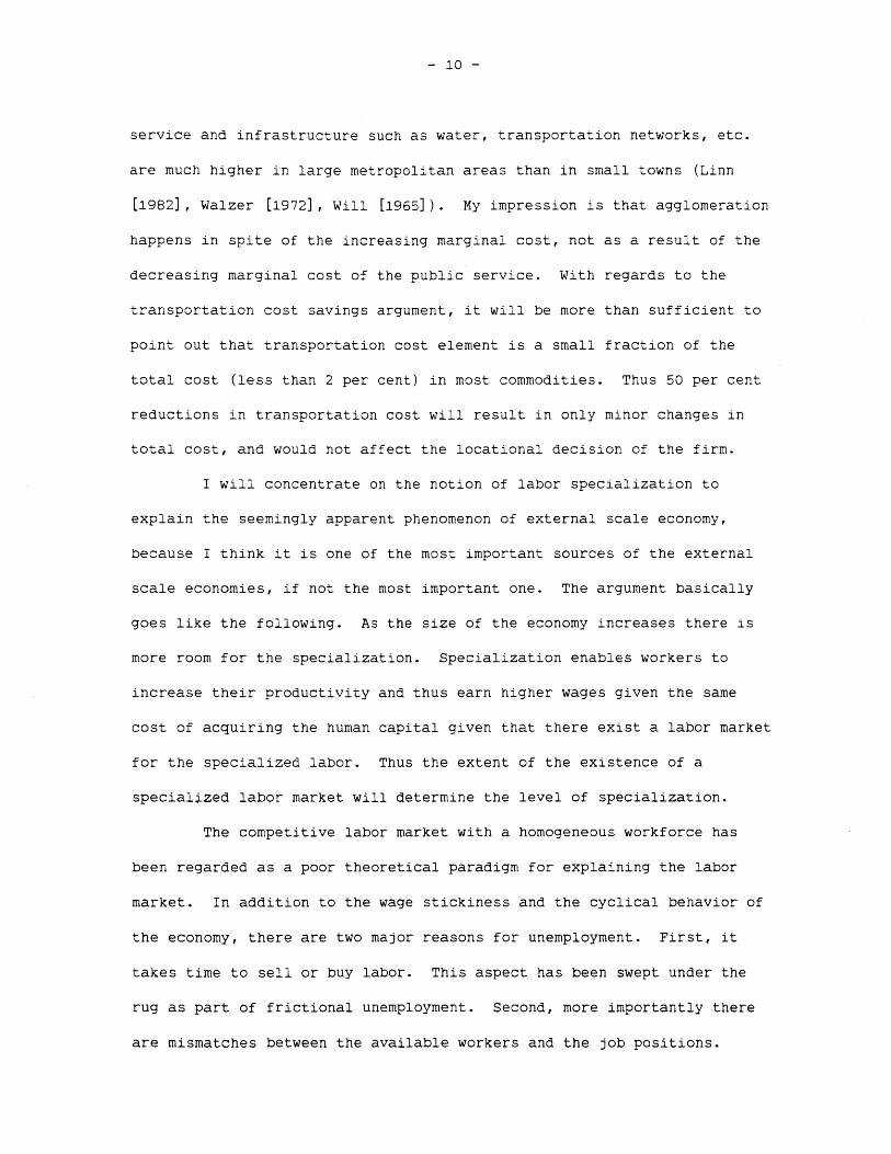
service and infrastructure such as water, transportation networks, etc.

are much higher in large metropolitan areas than in small towns (Linn

[1982], Walzer [1972], Will [1965]). My impression is that agglomeration

happens in spite of the increasing marginal cost, not as a result of the

decreasing marginal cost of the public service. With regards to the

transportation cost savings argument, it will be more than sufficient to

point out that transportation cost element is a small fraction of the

total cost (less than 2 per cent) in most commodities. Thus 50 per cent

reductions in transportation cost will result in only minor changes in

total cost, and would not affect the locational decision of the firm.

I will concentrate on the notion of labor specialization to

explain the seemingly apparent phenomenon of external scale economy,

because I think it is one of the most important sources of the external

scale economies, if not the most important one. The argument basically

goes like the following. As the size of the economy increases there is

more room for the specialization. Specialization enables workers to

increase their productivity and thus earn higher wages given the same

cost of acquiring the human capital given that there exist a labor market

for the specialized labor. Thus the extent of the existence of a

specialized labor market will determine the level of specialization.

The competitive labor market with a homogeneous workforce has

been regarded as a poor theoretical paradigm for explaining the labor

market. In addition to the wage stickiness and the cyclical behavior of

the economy, there are two major reasons for unemployment. First, it

takes time to sell or buy labor. This aspect has been swept under the

rug as part of frictional unemployment. Second, more importantly there

are mismatches between the available workers and the job positions.

- 11 -

Since the demand for output and the production technology is constantly

changing and there are substantial human capital investment are required

to adjust to the new labor demand, the workers' decision to invest in

human capital should take into account the uncertainty of the future

labor market. The same type of argument applies to the firms decision to

hire workers. Firms are faced with fluctuating demands for output.

Since hiring and training costs are substantial and the quality of the

new workers are uncertain, firms' hiring decision should take into

account the nonhomogeneity of the labor pool.

To make the exposition clear and simple, let us suppose a well

defined market in which the outputs are either homogeneous or very close

substitutes for each other. Also consider two groups of agents in the

market, namely workers and firms. Workers have to accumulate human

capital and sell their labor to firms in the factor market. The worker

chooses how much he wants to invest in human capital, and the level of

specialization. The choice among occupations is not allowed since it is

assumed that there is a single market in which all the workers have the

same occupation. It is common knowledge (in the game theoretic sense)

that more specialized workers who can perform narrower range of tasks

with higher productivity than more general workers given the same human

capital investment. The level of specialization that a worker chooses

will depend on the wage differentials between the generalist and

specialist and the relative probability of being employed. For example,

a worker wants to be a specialist if the probability of being employed as

a specialist is same as a generalist.

Labor demand is also determined by the two market parameters:

the wage differentials and the relative probability to find desired

- 12 -

workers. If the wage differentials are small, and specialists are widely

available, that is, the probability to get a specialist is not very much

lower than that of getting a generalist, then firms will want to have

more specialists. Higher demand for specialists will in turn raise the

wage differentials and lower the probability of finding a specialist. In

a single good market, the size of the market can be measured

unambiguously by either the number of workers or the level of output. In

equilibrium, we would expect a higher specialization in a larger market,

which is roughly consistent with the casual empiricism. For example,

there are various medical specialists in a large metropolis, while all

the doctors in a small town tend to be general practitioners. I would

like to emphasize that the gains in the production efficiency is external

to the individual agents of the market, i.e. individual agents can

influence the market by only a small amount.

II. Literature Survey

We can classify the literature on urban size and distribution

into the three major categories. A first approach, which is popular in

the regional science and economic geography, focuses mainly on the

distribution of city sizes. Central place theory, first proposed by

Christaller and then developed further by Losch, tries to examine the

economic and geographic hierarchy of different size of the cities. The

theory envisions a system of cities as a hierarchy, with a small number

of large cities and a large number of small cities forming a multi- level

hierarchy. On the contrary, the studies on the statistical regularity of

distribution of cities view the size of cities as a continuum, and try to

- 13 -

find statistical laws which govern the observed distribution of city

sizes. The first major work in this thrust is the so-called "rank-order

rule", popularized by Zipf in the early 1940's. There are numerous

studies in this framework, using more general functional forms of Pareto

distributions or log-normal distributions. There have been some efforts

to relate the central place theory to the statistical regularities. The

pioneering efforts in this area are Beckman [1968] and Simon [1955].

The second approach, which is mostly pursued by the economists,

emphasizes the productive efficiencies of city sizes. The basic

hypothesis in this line is that there is a productivity gain, at least to

a certain level, in larger cities. The theories propose various reasons

for the scale economies. Earlier theories emphasized the savings in

transportation cost from locating firms closer to each other. Recent

theories emphasize cost saving in social indirect infrastructure , labor

pools, and information. The major tool in empirical studies is, however,

the aggregate production function using the cross-sectional data sets

across the different urban areas.

The third approach asks more policy-oriented questions, namely,

whether there is a most efficient size of city, what are the sources of

efficiency gains and the losses of urban con.centrations, and how does the

optimal city relate to national economic development strategies. These

questions are more often raised among the practitioners of economic

development and urban and regional planning. I will follow the order of

these three major approaches in reviewing and evaluating the strengths

and weaknesses of the relevant literature.

1. Theories of distribution of city sizes

- 14 -

In his classic study of Southern Germany, Christaller [1966

English translated version] assumes a homogeneous plain over which

resources are uniformly distributed. A city's prime economic function is

assumed to be service to the surrounding hinterland, including, except in

the case of the smallest size cities, the lower level (smaller) cities.

The market area thresholds for the various goods and services are

different for several reasons. The structure of transportation costs is

different. There are different levels of scale economies in production.

The size and the pattern of demand would also vary among the different

products and services. The smaller that the threshold level of a

particular good or service is, the smaller is the size of the city needed

to perform the distributional role for that good or service. As the

larger city always includes similar functions to those lower level

cities, the equilibrium will be characterized geometrical networks of

city hierarchies.

This model predicts that cities with the same hierarchy level

will have the same population. This is not.observed in reality. There

is a continuum of city sizes rather than discrete levels of city sizes.

The "rank-size rule" approximately characterizes this feature in a

particular way. It states that for the cities within a country the

product of the city population and the rank of its population is

approximately equal to a constant, which is the population of the prime

city. This regularity has been remarkably confirmed in many countries in

spite of the differences of definition of cities, level of economic

developments, and so on among countries.

The "rank-size" rule is only a particular case of a = 1 in a more

general form of Pareto distribution

- 15 -

R = A S-a, (2.1)

where R is the rank of the city, S is the population of the city, and A

and a are constants. Although values of the coefficient a, commonly

called the Pareto coefficient, differs substantially with alternative

definitions of cities, the regularities are remarkable in many countries

(Rosen and Resnik [1980]). As Simon [1955] has shown, the Pareto

distribution is an equilibrium state of the stochastic process in which

the growth rates of population are uncorrelated with the city sizes. The

underlying stochastic process of uncorrelated growth rates and city size

is similar to a notion known as Gibrat's law in firm size distribution

studies.

There seems to be secondary regularities observed in the in the

studies of firm size and city size distributions, namely upward or

downward concavities. The Pareto distribution should be plotted as a

straight line in a log-log graph. However, many developing countries and

some developed countries such as France show an upward concavity (that

is, the second derivative is positive), in which the largest cities have

more population and the medium cities have less population than was

predicted by the Pareto distribution. Ijiri and Simon (1974] have shown

that if the growth rate is auto-correlated (that is, current values are

correlated with past values), then the curvature appears in the steady

state. For example, if growth rate is positively auto correlated, then

the distribution will show the upward concavity. Vining [1976] has shown

that the curvature may result from the correlation between the growth

rate and population size. This has an interesting behavioral implication

- 16 -

in the distribution of city size, namely, if there exists a scale economy

of city sizes, i.e., if larger cities are more efficient than smaller

cities, then the larger city will attract more population than the

smaller city, ceteris paribus. So the growth rates of the large cities

will be larger than the small cities, which means growth rate and

population are positively correlated. With positive correlation, we

would expect the upward curvature. One might want to use this

characteristic to test the existence of the scale economy of cities. But

city size distribution may well also depend on administrative

characteristics, political power distribution, and other aspects as well

as on economic factors. Thus, the mechanical application of the

stochastic process theory to the derivation of efficient city size would

not be appropriate.

Beckman [1958] has published an earlier effort to relate the

central place hierarchical model with the Pareto distribution of city

sizes. The key assumption he makes besides the central place theory is

that the population of the city is proportional to the population of the

market area it serves including the city itself. With the two

assumptions, he derives the size of the population and the population

served increase exponentially with the level of city in the hierarchy.

Solving eq.(2.1) for S gives population of the "rank-level" as an inverse

exponential function of the "rank-level". Beckman then approximates the

step function to the continuous function by choosing a mean at each

rank-level to show the rank size rule. There is a criticism by Parr

[1969] on the ground that the population served is not exactly treated in

Beckman [1958], and the correct formulation does not yield an exact

"rank-size rule". But I think the major criticism should concern the

- 17 -

approximation of the step function. If the number of lower level cities

for each higher level city is 3, which was suggested by the original work

of Christaller, the number of cities of 6th highest level is 256.

Choosing one city out of 256 to approximate the step function to a

continuous function seems quite crude. Besides, the approximated

continuous function has 6 or 7 points (number of levels). This makes the

approximation argument difficult. In my opinion, the effort to link the

two different theories of city size distribution seems not been

successful. Besides, the pure game of stochastic process does not

illuminate very much in the urban concentration and efficiency questions

because of the lack of behavioral grounds of the theory.

2. Scale economies of city sizes

It has been widely claimed that there exists a scale economy of

city sizes. Similar notions such as external economy, localization

economy, backward and forward linkage, and agglomeration economy have

constantly attracted the research interests of urban economists, regional

economists, urban geographers, and city planners. However, there seems

to have been either some confusion or ambiguity over why and how the

production efficiency is improved (at least to certain extent) with the

size of the city. Carlino [1978, 1980] has provided three useful

distinctions in the concept of scale economies of cities, namely,

internal returns to scale at the plant or firm level, localization

economy, and agglomeration economy. I will arrange the discussion

following his framework.

First, it is conceivable that there is a scale economy in the

plant level, i.e., decreasing average cost with respect to the quantity

- 18 -

produced. This notion is widely recognized, although highly

controversial, in the production economics area. Although there are a

number of industries which in reality seem to exhibit increasing returns

to scale over a reasonable range of production (for example, public

utilities), the linkages between the internal returns to scale and the

existence and the growth of cities are not very clear. Henderson [1974]

provides a theoretical explanation of the size distribution of cities

along this notion. Under the assumption of complete specialization and

increasing returns to scale, he manages to demonstrate a size

distribution of cities determined by the level of scale economy. But

complete specialization to a single industry for a reasonably large city

is obviously a very strong assumption. The largest single industry

defined by the two-digit industrial classification, in highly specialized

U.S. cities such as Detroit and Cleveland has less than 30 per cent of

the total employment of the metropolitan area.

A similar idea has been investigated in the local public sector,

namely, whether there are scale economies of the municipal services. Not

surprisingly the results are quite problematic. For example, Hirsh

[1959] claims that expenditure per capita did not vary significantly,

while Schamndt and Stephens [1960] suggested that the service index is

positively correlated with population size although per capita

expenditure was not significantly correlated with city size. Walzer

[1972] claims, on the contrary, that a negative relationship between the

service indices and the city size was found while per capita expenditure

was not correlated with population. For one thing, the right index for

the municipal services are not obvious in many cases. Many studies used

per capita expenditure as a proxy for the level of service provided.

- 19 -

There are many factors to determine the per capita expenditure. Demand

for public service might be substantially different from one community to

another. The cost of providing the same service level may be quite

different depending on the natural conditions (climate and geography),

social environment (income, age, religion, race distribution). So the

comparison of expenditures seems to be close to be meaningless. Some

studies have used a custom made index for the service level, which could

be quite controversial. In summary, the existence of scale economies in

government service seems quite inconclusive.

The localization economy, Carlino's second notion of increasing

returns to scale in urban areas, is due to the horizontal and vertical

linkages among industries. Many firms in the same industry can share the

cost of infrastructure (roads, ports, electricity, etc), information, and

the specialized labor pool. While traditional location analysis (both

theories and empirical studies) emphasize cost savings of the physical

inputs, some recent studies focus on the importance of information and

availability of specialized labor (Carlton [1969]). Vertical linkages

are mainly discussed in a planning context to take advantage of

transportation cost in the industrial complex development (Richardson

[1977]). The notion of localization economies has some appeal as an

explanation of the existence of large cities, because it can demonstrate

the scale economy of a city even with the decreasing returns to scale in

each plant.

The third notion, agglomeration economy or urbanization economy,

is an extension of the localization economy into a more general form. In

his old but still insightful book, Vernon [1960] provided plausible

causes of the agglomeration economy of New York metropolitan region;

- 20 -

"enormous amount of rental space, extremely diversified labor force,

varied group of suppliers of industrial material and services, and

extensive transportation facilities ... (which) had been the

consequences of its earlier growth of a century or so..." The

agglomeration economy is a genuine form of externality which is mainly

due to the spatial accessibilities to the diversified and specialized

urban resources.

In the mid 1970's, there were some efforts to test the existence

of scale economies of city sizes by using aggregated production function.

These studies were stimulated by Fuch's [1967] finding that workers in

large cities are paid more than the workers in small cities ceteris

paribus. One possible explanation for this is that there is a efficiency

gain in the larger cities so firms in the large cities can outbid the

wages in the smaller cities. Sveikauskas [1975] estimated that doubling

the city size will yield the 6 percent increase of productivity. Segel

[1976] tried to distinguish the agglomeration effect and the increasing

returns to scale (a very similar notion to that of localization economy)

by having the estimation equation with both shift parameters and the sums

of parameters in the Cobb-Douglas aggregated production function not

equal to one. And he claimed that the sum of the parameters are not

significantly different from one, while the shift parameter of population

over 2 million is significant. He concludes, on the basis of this, that

agglomeration is more evident while scale economy is not strong. A

critical review and reestimation of the production function by Moomaw

[1981] suggested that the Sveikauskas''s result was overestimated because

of the overestimation of capital stock in the older cities. His estimate

is that 2.5 percent of increased productive efficiency is achieved by

- 21 -

doubling the population. But he agrees with both earlier writers that

there is an efficiency gain.

The only serious effort, to my knowledge, to identify the

localization economy and agglomeration economy is done by Henderson

[1983]. He defines the localization economy as a productivity increase

due to the number of employees in the same industry defined in two digit

SIC categories, and agglomeration economies as due to the total

employment in the metropolitan area. His results are basically for the

localization economies. Also he finds that the localization economies

level off quite soon. But he confined his study in the manufacturing

industry only, in which industrial linkages and availability of workers

pool tend to be more important. Presumably, service industries,

including retailing and wholesaling, require more face to face contact

and fast digestion of continuous information flows. Thus his conclusions

for localization economies are exaggerated while those agglomeration

economies are underestimated if we include all types of economic

activities in cities.

Another promising line of research is the search based

agglomeration (e.g. Pascal and McCall [1980] and Stuart [1979]). The

idea here is the agglomeration occurs because of the search cost savings

in buying or selling product and in hiring and purchasing specialized

labor and input. The most notable search based agglomeration occurs in

the retailing clusters such as shopping malls. The imperfect

information, which can only be reduced through the search in the market

may be the micro foundations for the urban agglomeration.

So far, I have mainly focused on the production efficiency of

larger cities. Besides the production efficiency, consumption diversity

- 22 -

could be another source of agglomeration economy. For example, suppose

there are two cities of different sizes with the same productivity, i.e.,

there are no productivity gains in the larger city. And if a producer

produces different varieties of the same good, then the larger city can

produce a larger number of different varieties. If consumers care about

the variety of goods as well as the price, then the consumers in the

large city can attain higher levels of utility with the same income.

This will attract immigrants from the smaller city. This type of

consumption efficiency gain never has attracted any serious analysis in

the past literature, however.

3. Optimum city size and decentralization policies

In any optimal city model, a trade off is postulated between some

sort of efficiency gain and an increase of social cost. It is very

curious, however, that what kind measure of city size we are talking

about. In most studies, population is regarded as the city size. But

other alternative measures might be important and interesting as well.

For example, can we make any sense by comparing a city in India with

population of one million with a city in U.S.A. with the same

population. Regional output could be an interesting measure of a city's

size. In some studies, physical size such as the diameter of a city has

been discussed as a measure of city size (e.g. Henderson [1975]). As

the population density varies a great deal among different countries, the

discussion of physical size should also be useful.

In the previous section, I have discuss the possible sources and

analytical and empirical studies on the economies of scale. There are

certainly diseconomies of scale associated with the city size. Let me

- 23 -

list the possible candidates, then elaborate one by one; higher land

rents, congestion, pollution, worsening of social environment such as

crime, social infrastructure and provision and financing of local public

services. In an open system of cities, any desirable or undesirable

characteristics of a site will be capitalized into the land value. These

will include non-market goods such as pollution as well as the marketable

attributes such as cost savings of transportation. If the economic

agents and factors are perfectly mobile, then the utility level and the

return on factors will be equalized -everywhere in the economy. In this

case, land value capitalization would not affect the efficiency. If some

things are immobile in the economy, the land rent will ensure efficient

allocation when all externalities are internalized. With the presence of

the externality and impossibility of marginal pricing of externality and

public goods, the land value capitalization would not lead to an optimal

city size. The direction of market force is ambiguous.

Pollution and congestion cases seem more clear. Assuming the

level of pollution or congestion is an increasing function of the number

of people in the city, and the cities market price is short of the social

marginal cost, a city's population will be likely to be overconcentrated.

As the price that the individual perceives does not include the social

cost imposed by the individual, the individual acts according to the

equalization of average cost and average benefit, which in turn will lead

into the overconcentration. The provision of public services in urban

area has been regarded as another reason for this overconcentration. As

transfer payment or public services to low income groups of people in

urban areas and more likely to exceed those in rural area, there is a

incentive to move into the city, particularly in the case of low income

- 24 -

groups. The effect of the fragmented local government may work in the

other way. Thus, competition among governments may prevent local

governments from engaging in income redistribution programs, and this

will weaken the previous claim.

The question of whether the competitive market system will lead

to too large or too small populations (when compared with the optimal

size) is problematic. If there exists only scale economies not

diseconomies (such as congestion and pollution), then it is not difficult

to see the equilibrium city size is too small. If there exist only

negative externalities, the opposite will be true. But with the two

forces both -existing, one has to look at the relative strength of the

positive and negative externalities. Another complication has something

to do with the financing of the public goods in the local government

sector and with the land value capitalization. The first question is,

then, whether the optimal city size exists. If agglomeration economies

always outweigh negative externalities, then the optimal size will be

infinite and every city is too small. But this case is unlikely because.

the plausible gains will be outweighed by agglomeration losses. Marginal

social benefit will be eventually level off, since, the advantages of

both production efficiency and consumption efficiency tend to go away

when the city becomes "large enough". Marginal savings of transportation

cost, search cost, and input costs are achieved by sharing the common

facility or labor pool are not likely to decline substantially after the

city reaches certain size. On the contrary, marginal social cost will

more likely be an increasing function of the city sizes. As an analogy,

the highway congestion level increases drastically when the traffic

volume increases beyond physical capacity. Costs of pollution seems to

- 25 -

follow the same pattern. So it is likely that an optimal city size

exists. This does not imply that there is a universal, optimal city size

among all urban areas at all times. Cities are historical products. And

they are in different geographic and economic settings. So the optimal

city size of a given city may be drastically different from another.

Besides, the optimal size of a given city is subject to change depending

on the technology. For example, levels of pollution and congestion are

not completely exogenous. With technological improvement and public

investment, the marginal social cost curve may shift.

Finally, I will briefly comment on the observed degree of urban

concentration with the level of economic development. Wheaton and

Shishido [1981] have found that the degree of urban concentration is a

inverse of the U-curve, namely, the urban concentration becomes higher in

the earlier stage of economic development and lower in the later stages.

This is analogous to the Kuznets hypothesis of income distribution and

the Williamson's hypothesis of regional income disparity, namely, income

distribution (size distribution in Kutznets and regional disparity in

Williamson) becomes more skewed in the earlier stage of the economic

development and less skewed in the later stage. This can be justified by

many stories, one of which is the Hirshman's "spread and backlash"

effects. Rosen and Resnik [1980] also support the inverse U-curve

hypothesis in their city size distribution study, although they did not

say this explicitly.

However, these studies suffer from the usual criticisms of cross

national comparisons. First, the countries are not a homogeneous group,

their definitions of cities are different and their physical structures

of cities are different. Second, cross country comparisons do not imply

- 26 -

time series changes. That is to say, we cannot infer from the empirical

observation that if a country becomes more developed, then it will be

more decentralized and so on. Third, the real outcomes of city

distributions are also affected by the urban and regional policy and

general economic development strategy. Namely, many countries which have

been successful in growing faster in the last decades are

industry-promoting countries which push toward manufacturing, which is

mainly urban based. Therefore, although the observation that middle

income countries are more spatially concentrated than the lower and upper

income countries seems to be true, it should be interpreted with caution.

III. Thesis Outline

In this section, I will briefly sketch the outline of the

dissertation. Footnotes and figures appear at the end of each chapter.

In chapter II, two models of agglomeration economies will be presented

and analyzed The external economies are generated mainly from the fact

that with larger market size, labor specialization can occur more fully

to exploit the productive efficiency of individual worker's skill which

comparatively more efficient than others. Individual firms are assumed

to have constant marginal productivity technologies with some minimum

efficient scale so that they exhibit increasing returns to scale.

However, its ability to hire such workers will be limited by the size of

the local labor market. The main results of chapter II is that average

labor productivity will rise as the size of the market increase given the

minimum efficient scale, the marginal productivity, and the loss of

productivity due to the mismatch between the worker and the job.

In chapter III, workers are allowed to choose the level and the

- 27 -

extent of his human capital. The former will be called intensive human

capital, and the latter will be called extensive human capital

respectively. An extension of the bargaining model in chapter II will be

analyzed. In a larger market, firms will have technologies which require

more specialized labor, since the labor pool is large and diverse enough

to support such specialized production. By the same token, workers will

be more specialized (i.e., they will have more intensive and less

extensive human capital), since there is a higher probability to get the

better matching job when the jobs in the market are more diverse.

The analyses in Chapter II and III suggest that regions will

follow the divergent growth paths. If the scale economies prevails, then

the real wages will be higher in the larger cities, which in turn,

attract more people with same or higher return on capital. If a city has

a slightly larger endowment then agglomeration of the larger city will

occur. Larger cities become larger and smaller cities become smaller.

In reality, the extreme case of agglomeration will not occur because of

the following stabilizing forces.

First of all, the external scale economy may peter out after a

certain level. In this assumption, a city will grow up to a point after

which small cities will grow faster to exploit the efficiency gain of the

growth. Second, spatial concentration will result in the higher rents on

land, which will jack up the living cost as well as the production cost.

Also the cost to provide urban services, such as water, sewer,

electricity may increase rapidly with the growth. So workers will demand

higher wages, and relative advantage to locate in larger cities become

less attractive. Third, spatial concentration will also lead into the

non-pecuniary externality. In larger cities, the external diseconomies

- 28 -

of scale such as congestion and pollution may be rapidly rising with the

city sizes, which will lead into the efficiency loss in larger cities.

So steady state will have large cities as well as the small cities.

In chapter IV, negative externalities will be incorporated into

the model in order to discuss optimal city sizes, efficiency

characteristics of systems of cities, and possible policy roles. The

presence of externalities, in general, result in an inefficient market

solution, and there is a room for the public action to improve the

efficiency. Policy alternatives are quite diverse ranging from tax

incentives to forced decentralization, and social consequences of the

policies may be far reaching. Rapid urbanization in many developing

countries in the past three decades create a great deal of tension in the

traditional social structure and life style. It is hoped that the model

would be a useful guideline to evaluate such alternative policy measures.

CHAPTER II

Labor Specialization and Agglomeration Economies

I. Introduction

One of the major characteristics of a modern economy is that

diverse and specialized economic activities are concentrated in small

geographical areas. The process of concentration of economic activities

is loosely referred as urbanization, in which the emphasis is placed on

the concentration of people. Since human activities are limited by

distance, the major portion of the activities of an urban man occurs

within the metropolitan area in which he resides. Moreover, a typical

urban man is engaged in a very specialized production activity. Only a

small fraction of his output will be consumed by himself. Most of his

consumption needs are satisfied by goods and services produced by others.

In fact, it is not very difficult to recognize the close

inter-relationship between the concentration of economic activities and

specialization. Let us take an example for illustration. Think of a

small island and its sole resident, say Robinson Crusoe. He must produce

various goods and services in order to survive. He must raise crops,

cook food, make clothing, build a house, and so on. His energy should be

devoted to many productive activities, and he needs learn how to do all

of those things.

Suppose, for some reason, a group of people arrived at the

island. Moreover, let us assume that some people are naturally good at

- 30 -

hunting, while others are good at baking, and so on. Since there is a

cost involved in learning how to do anything, it would be beneficial to

specialize in certain productive activities and to trade the various

outputs among the village residents. Our Robinson Crusoe decided to

specialize in baking. Now since he has only one production activity to

worry about, he can bake more bread, more quickly, than in the previous

self-sufficient situation. In other words, his average product of baking

increased as a result of specialization. But notice that he could not

specialize in baking before the other people arrived. He can only

specialize when there are other people around to provide various goods

and services other than bread. What I have described is an illustration

of Adam Smith's doctrine that "the division of labor is limited by the

extent of the market" (see Stigler [1959] for more discussion).

Urban agglomeration has long been explained by the cost savings

in transportation and/or in sharing the urban infrastructure. A typical

theory is that producers can save in transportation cost of inputs and/or

outputs by locating at the points near to where they purchase inputs or

sell outputs. In general, economic agents can reduce the cost of

transportation or social infrastructure by locating close together.

However, the transportation cost typically comprises only an

insignificant fraction of the total cost of most of the goods and service

produced in an urban area. Also providing a given level of public

service in a large metropolitan area costs many times more than in small

or medium cities (Linn[1982]). This chapter presents an alternative

argument that specialization of production activities is the major source

of urban agglomeration.

Although geographical proximity plays an important role in the

- 31 -

process of urban agglomeration, the argument is that geographical

proximity enables producers to specialize, and thus to increase

productivity. Given the usual social practice that workers commute back

and forth between their residence and workplace on a daily basis,

specialization would be limited by the size of the urban area in which

daily commuting is possible. Although average productivity will be

increased by adopting more specialized and roundabout technologies, such

technologies can only be adopted when the market is large enough so that

they can be supported by the activities of other agents in the market.

Some studies have tested the existence of scale economies of city

size by using aggregate production functions. These studies were

stimulated by the Fuch's [1967] finding that workers in large cities are

paid more than workers in small cities ceteris paribus. All the studies

which I am aware of conclude that there do exist scale economies in city

size (Sveikauskas [1975], Segel [1976], Moomaw [1981], and Henderson

[1983]).

This chapter presents models of agglomeration economies.

Localization economies and urbanization economies are not distinguished

(see Carlino [1979] for such distinction). The literature about product

differentiation emphasizes the availability of the wide variety of

products in the modern economy. The utility of consumers will be

increased either by having more variety (Dixit and Stiglitz [1979] and

Spence [1976]) or by having the variety which is more similar to the

ideal variety (Lancaster [1979]). The utility gain through the

consumption of diverse products will not be discussed in our models.

Rather we will focus on the production side of the economy by assuming a

competitive market of homogeneous output.

- 32 -

Another important point which our model does not address is that

the worker's human capital investment decision will be made on the basis

of the availability of jobs which require such specialized skills. In

the highly specialized modern economy, the choice of the extent of

specialization is as important as the level of human capital investment

to the worker's decision, since the stream of future earnings will depend

upon the extent of his specialization as well as upon his skill level.

The models presented in this chapter excludes the possibility of

endogenous human capital investment decisions.

We shall abstract the urban labor market from the spatial

setting. The urban land market and other consequences of concentration

of economic activities (e.g. congestion and pollution) will be ignored.

The movement within the city is assumed to be costless. Movements

between the urban market is prohibited. In short, we shall analyze the

aspatial closed labor market.

Two models will be presented in this chapter. The first model is

a signalling equilibrium model1, and second one is a bargaining

equilibrium model. The set-ups are quite similar. The major difference

is how the wage is determined. In the signalling equilibrium model, wage

is determined by firms on a take-it-or-leave-it basis. In the bargaining

equilibrium model, wage will be determined by an axiomatic bargaining

solution between workers and firms. The signalling equilibrium will be

analyzed in section II. The bargaining equilibrium will be analyzed in

section III. Conclusions are offered in section IV.

II. Signalling Equilibrium

- 33 -

1. Assumptions

Let us consider a closed economy of a continuum of

workers-cum-consumers with aggregate size N. Workers are indexed on a

circle of a unit length with uniform density. Since the circle has the

unit length, the density is also N. The index represents the worker's

skill characteristic. Sometimes we will call the index location and the

difference between two indices distance. Notice that terms like

"location" and "distance" do not have any geographical meanings. There

is no a priori superiority or inferiority among workers' skills. The

size of the difference between the indices of any two workers represents

how different they are. Obviously the difference ranges from zero to one

half. Every worker supplies one unit of labor provided that the net wage

offer is greater than or equal to his reservation wage.

We assume that all the workers in the economy have the same

reservation wage wo. The reservation wage reflects either the utility of

leisure or the domestic productivity of a worker. In the following

discussion, wo is interpreted as domestic productivity which a worker

gets when he works for himself. We call this situation self-sufficient

autonomy.

There are also firms in the economy. Since we do not allow

multi-plant firms, we can identify firms without any confusion. Firms

are assumed to produce homogeneous goods, which are sold in the

competitive output market. The output price is normalized to one.

Technologies are also indexed on the unit circle. The index of the

technology represents the most productive skill characteristic. The

firms can choose their technologies in the long run, but not in the short

run (long run and short run will be defined later). Since the

- 34 -

technologies only differ by their most productive skill characteristics,

we can unambiguously identify the firm with its most productive skill

characteristic. We shall call the characteristic the firm's location.

The critical assumption in the signalling equilibrium is that the

firm cannot identify workers' location, while they know the firm's

location. Thus, we assume that there is a unique firm-specific signal

associated with its most desirable skill characteristic. The firm will

hire any workers if they have its signal. If a worker wants to work for

a particular firm, he has to invest in order to acquire the firm-specific

signal (see Spence[1974] for more discussion on signalling). The cost of

acquiring the signal is assumed to be a monotonically increasing function

of the difference between the worker's index of skill characteristic and

the firm's index of most desirable skill characteristic. As we analyze

the behavior of a representative firm, and workers who have skill

characteristics similar to the firm's most desirable characteristic, we

will choose the firm's index as zero without loss of generality. Then we

could denote the difference as t, 0 < t < .5. In particular, we will

assume that the cost of acquiring the signal c 1 (t) has the following

properties 2:

c1 (0) = 0 (2.1.a)

c 1'(t) > 0, for 0 < t < .5 (2.1.b)

c 1"(t) > 0, for 0 < t < .5. (2.1.c)

To avoid the complication of substitution between productive

factors, we shall assume that labor is the only productive factor. The

firm has, what we call, roundabout technology, with the minimum efficient

- 35 -

scale (M) and the constant marginal product (b). It is clear that the

technology has an increasing returns to scale. More specifically, we

assume the production function has the form of:

Y = 0 if X < M (2.2.a)

b (X - M), if X > M, (2.2.b)

where Y is output, and X is the labor input normalized to the equivalent

labor with the firm's most desirable skill characteristic. The firm

hires only workers who possess the firm's required signal. Since the

firm cannot distinguish the workers in terms of their skill

characteristic endowment, the wage offer will be the same for workers

with the same signal. But the possession of the signal does not increase

the worker's productivity. We assume that the productivity is a

decreasing function of the difference between the worker's skill

characteristic and the firm's most desirable characteristic. More-

specifically,

x = x(t) (1 - c 2 (t)/b) (2.3.a)

c 2 (0) = 0 (2.3.b)

c 2'(t) > 0, (2.3.c)

where x(t) is the amount of labor with the difference t, and x is the

normalized labor unit. c 2 (t) is the value of the lost product due to the

difference. Total labor input (X) is just the sum of the normalized

labor (x) of the workers.

- 36 -

We will call the situation short run when there is a fixed number

of firms (m). As we have indicated, firms do not change their location

in the short run. Wage offer is the only short run decision variable of

the firm. We shall concentrate only on the symmetric equilibrium. By

symmetry, we mean that all the firms offer the same wage and the

distances between any two neighboring firms is the same. Thus, we have:

2mH = 1, (2.4)

where 2H is the distance between any two neighboring firms. The short

run profit of the firm will be:

dP(d) = b[2Nd - M] - 2N[wd + 9 c 2 (t)dt]. (2.5)

The variable d will be called the market area of the firm. All the

workers who have the characteristic difference less than d will work for

the firm. If there is no gap between the neighboring market areas, then

we have:

d = H. (2.6)

If there is a positive short run profit, then entry will occur.

If short run profits are negative, firms will exit. Assuming that there

are no costs of relocating firms, competition among firms will result in

that all the firms get zero profit. The situation that the number of

firms (m), and thus, the distance between the neighboring firms (2H) are

determined endogenously by the zero profit condition will be called long

- 37 -

run.

We are mainly interested in the long run symmetric Nash3

equilibrium. A firm will choose the location and wage offer. A worker

will choose the firm he will work for by maximizing his net wage (wage

offer minus his cost of acquiring the firm-specific signal), provided

that it is greater than or equal to the reservation wage w.. The firm

makes its wage offer by assuming that other firms' wage offers will be

held constant. In the game theory language, firms will play Stackelberg

leader towards workers and play a Nash strategy to the other firms.

Workers are Stackelberg followers to the firms.

2. Types of equilibria

Let us choose a representative firm i (1<i<m), and choose its

most desirable skill characteristic as the origin without loss of

generality. Since the situation is symmetric with respect to the two

neighboring firms, we will focus our attention on one side. In the short

run, our representative firm will choose wage offer w given that the

neighboring firm's (firm j, i<j<m) wage offer is w. As we see in Fig.

1, workers between firm i and firm j (O<t<2H) have three options: to

work for firm i, to work for firm j, or not to participate in the labor

market and to retreat to the self-sufficient autonomy. More

specifically, the behavior of the worker with skill characteristic t

(O<t<2H) is:

1. work for firm i, if w-c 1 (t) > max {w-c 1 (2H-t), wel (2.7.a)

2. work for firm j, if w-c1 (2H-t) > max (w-c1 (t), wo} (2.7.b)

3. not to participate in the labor market, otherwise. (2.7.c)

- 38 -

If b < wo (the marginal productivity of the roundabout technology

is lower than that of the domestic technology), then there will be no

labor market since workers will not work for firms which in turn cannot

afford to pay a wage higher than w0 . Every worker in the economy will

stay in self-sufficient autonomy. If b = we, the firms will get negative

profit since M > 0. Thus, we shall assume that b > wo hereafter.

Depending on whether the difference between the net wage and the

reservation wage of the marginal worker at the equilibrium is negative,

positive, or zero, we will have three different types of equilibria,

which will be referred to as, monopsony, monopolistic competition, and

kinked equilibrium following the tradition of Salop [1979]. As we can

see in Fig. 2, the three cases occur when the following conditions are

satisfied respectively:

1. Monopsony Case, if w - c 1 (H) < wo (2.8.a)

2. Monopolistic Competition Case, if w - c1 (H) > wo (2.8.b)

3. Kinked Case, if w - c 1 (H) = wo, (2.8.c)

where 2H is the equilibrium distance. If w-c 1 (H) < wo (monopsony case),

then some workers will not participate in the labor market at

equilibrium. Thus, the firm will act as a monopsonist. Suppose that the

representative firm raise its wage offer. Then some workers who did not

participate in the labor market before will work for the firm, if the net

wage offer exceeds the reservation wage. In the monopolistic competition

case (w-c1 (H) > wo), if the firm raises its wage offer with small amount,

then it will attract more workers away from the neighboring firm. Thus,

the labor supply to the neighboring firms will decrease whereas it would

- 39 -

not have changed in the first case. The labor supply curves of the two

cases would be different. The kinked equilibrium (w - c 1 (H) = wo)

occurs, because the labor supply curve will not be differentiable at the

kink. Since number of firms (m) and the distance between the neighboring

firms (2H) are endogenous in the long run, the conditions for the three

cases must be satisfied with equilibrium H's.

3. Monopsony case

In the short run, the representative firm maximizes its profit

(eq.(2.5)) by choosing its wage offer. However the firm's market area

(d) will be determined by:

w - c 1 (d) = wo. (2.9)

That is to say, the marginal worker is indifferent between working for

the firm and retreating to autonomy. Since by choosing its wage offer

(w), the firm chooses its market area (d) uniquely, we could regard the

firm's profit maximization problem as the choice of d. By solving

eq.(2.9) in terms of w, and substituting it into eq.(2.5), and

differentiating it with respect to d, we get the first order condition

for the profit maximization problem:

b - c 2 (d) = w + c 1'(d)d. (2.10)

This is the familiar profit maximization condition for a monopsonist.

The left side of eq.(2.10) represents the marginal value product (recall

that the output price is normalized to unity), and the right hand side is

- 4C -

the marginal outlay by hiring one more unit of labor. At ecuilibrium,

these two must be the same. In order to attract more workers to the firm

it is necessary to pay higher wage to all workers, since it is impossible

to distinguish among them. The second term in eq.(2.10) represents such

premium.

Since there may be gaps between the market areas of neighboring

firms, (i.e., some people may stay out of the labor market), the number

of firms will not be uniquely determined. The maximum number of firms m

is, however, 1/2d.

By imposing the zero profit condition, we get:

dbM/2N = c 1'd

2 + c 2d - f c2 (t)dt (2.11)0

Notice that the monopsony equilibrium is very unlikely to occur, because

eq.(2.9), eq.(2.10), and eq.(2.11) must be satisfied when there are only

two endogenous variables (w and d). It can only happen on the knife edge

of parameter values such that an additional condition must be satisfied

among them. For example, the monopsony equilibrium only occurs at a

point in one parameter, say wo, family of economies.

It would be useful to solve the model explicitly by assuming the

functional forms of c 1 (t) and c 2 (t). We will choose linear

specifications:

c 1 (t) = k 1t (2.12.a)

c 2 (t) = k 2t. (2.12.b)

The parameter k 1 tells you how expensive the signal acquiring

- 41 -

activity is, and the parameter kn tells you how much the technology

requires specific labor. High k1 implies that signal acquiring is

expensive. High k2 means that jobs require highly specific labor. With

eq.(2.12), the zero profit condition becomes:

bM/N = (2k-I+k 2 ) d2. (2.13)

Rearranging the terms, we get:

d = bM/(2k +k2)N (2.14)

m'= [1/2] i(2k j+k 2YP/bM (2.15)

w = b - [(k 1 +k 2 ) / j2k 1 +k 2 )] IbM/N. (2.16)

I have mentioned the extra constraint for the long run

equilibrium. To get this, we substitute eq.(2.14) and eq.(2.16) into

eq.(2.9). By doing so, we get:

(b-wo) 2 /b = (2k 1 +k 2 ) M/N (2.17)

In other words, if eq.(2.17) is satisfied, then we get the monopsony

equilibrium determined by eq.(2.14), and eq.(2.16). Comparative static

exercise cannot be performed since it is impossible to change one

parameter without changing others. For example, suppose that we change

the reservation wage(wo), then we have to change one more parameter(b,

k 1 , k 2 , M, or N) in order to satisfy eq. (2.17).

4. Monopolistic competition case

- 42 -

In the monopolistic competition case, the market area will be

determined by the following equation rather than eq.(2.9):

w - c1 (d) = w - c 1 (2H-d). (2.18)

That is to say, the marginal worker will be indifferent between working

for the representative firm (firm i) offering wage w and working for the

neighboring firm (firm j) offering wage w provided that the net wages are

equal. Solving eq.(2.18) in terms of w and substituting into eq.(2.5),

differentiating it with respect to d, and evaluating it at w = w (or d =

H)4, we get the first order condition for profit maximization 5:

b - c 2 (H) = w + 2c 1 '(H)H. (2.19)

Eq.(2.19) says that marginal value product should be equal to the

marginal outlay at equilibrium. It is very similar to eq.(2.10) except

that the second term on the right hand side is twice as great as that of

eq.(2.10). If the additional workers are already working for the

neighboring firm, then it is necessary to pay more in the monopolistic

competition case than in the monopsony case, because they currently

receive a wage higher than wo. The premium of the monopolistic

competition case is twice larger than that of the monopsony case because

of the symmetry of the net wage functions.

Imposing the zero profit condition, we get:

bM/2N = 2c1 (H)H2 + c 2 (H)H - f c 2 (t)dt.0

(2.20)

- 43 -

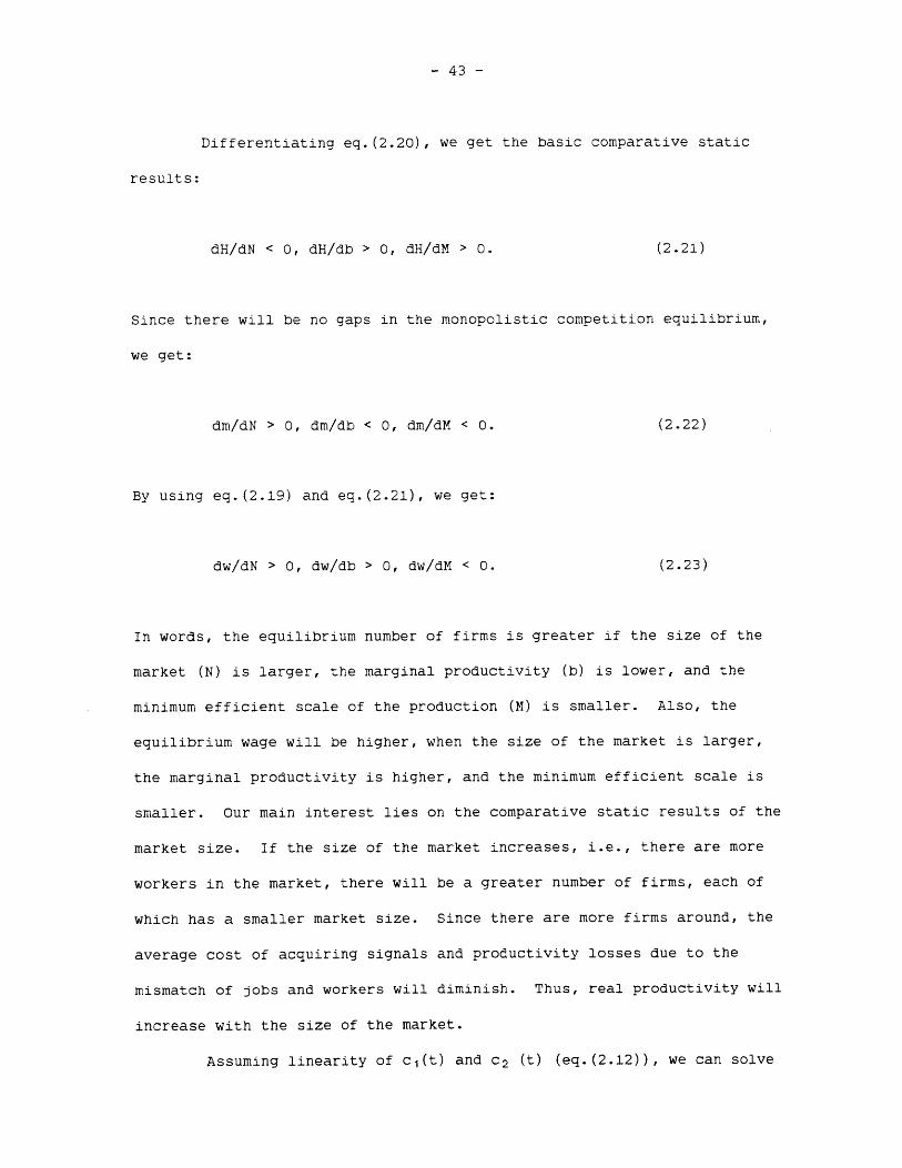
Differentiating eq.(2.20), we get the basic comparative static

results:

dH/dN < 0, dH/db > 0, dH/dM > 0. (2.21)

Since there will be no gaps in the monopolistic competition equilibrium,

we get:

dm/dN > 0, dm/db < 0, dm/dM < 0. (2.22)

By using eq.(2.19) and eq.(2.21), we get:

dw/dN > 0, dw/db > 0, dw/dM < 0. (2.23)

In words, the equilibrium number of firms is greater if the size of the

market (N) is larger, the marginal productivity (b) is lower, and the

minimum efficient scale of the production (M) is smaller. Also, the

equilibrium wage will be higher, when the size of the market is larger,

the marginal productivity is higher, and the minimum efficient scale is

smaller. Our main interest lies on the comparative static results of the

market size. If the size of the market increases, i.e., there are more

workers in the market, there will be a greater number of firms, each of

which has a smaller market size. Since there are more firms around, the

average cost of acquiring signals and productivity losses due to the

mismatch of jobs and workers will diminish. Thus, real productivity will

increase with the size of the market.

Assuming linearity of c 1 (t) and c 2 (t) (eq.(2.12)), we can solve

- 44 -

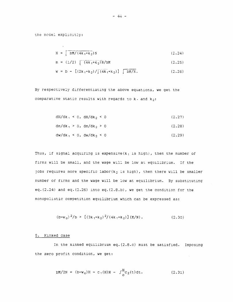
the model explicitly:

H = bM/ (4kj+k 2 )N (2.24)

m = (1/2) (4k-+k 2)N/bM (2.25)

w = b - [(2k 1+k 2)/J(4k +k2)] bM/N. (2.26)

By respectively differentiating the above equations, we get the

comparative static results with regards to k, and k 2 :

dH/dki < 0, dH/dk, < 0 (2.27)

dm/dki > 0, dm/dk 2 > 0 (2.28)

dw/dki < 0, dw/dk 2 < 0 (2.29)

Thus, if signal acquiring is expensive(k1 is high), then the number of

firms will be small, and the wage will be low at equilibrium. If the

jobs requires more specific labor(kn is high), then there will be smaller

number of firms and the wage will be low at equilibrium. By substituting

eq.(2.24) and eq.(2.26) into eq.(2.8.b), we get the condition for the

monopolistic competition equilibrium which can be expressed as:

(b-wo)2/b > [(3k 1+k 2 ) 2/ (4k 1+k 2 ) ] (M/N). (2.30)

5. Kinked case

In the kinked equilibrium eq.(2.8.c) must be satisfied. Imposing

the zero profit condition, we get:

bM/2N = (b-wo)H - c 1 (H)H - F c 2 (t)dt. (2.31)0

- 45 -

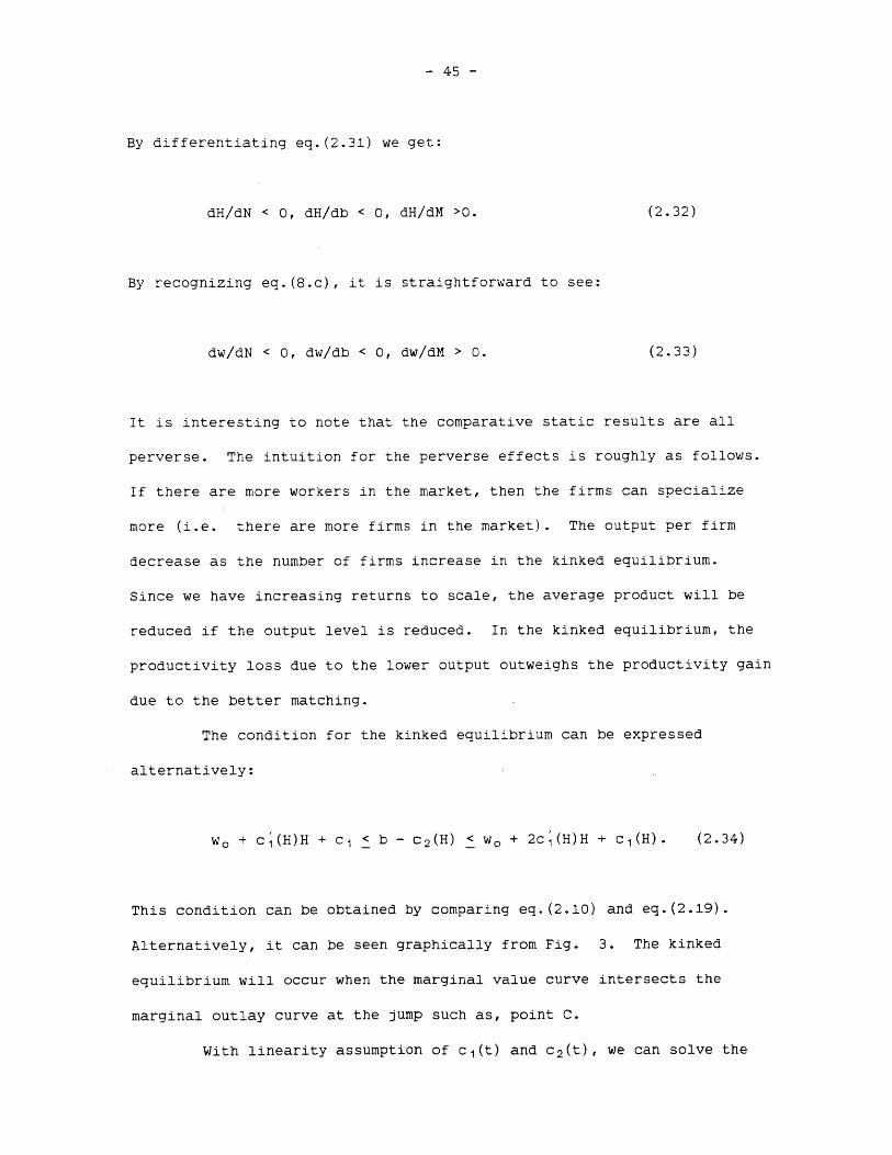
By differentiating eq.(2.31) we get:

dH/dN < 0, dH/db < 0, dH/dM >0. (2.32)

By recognizing eq.(8.c), it is straightforward to see:

dw/dN < 0, dw/db < 0, dw/dM > 0. (2.33)

It is interesting to note that the comparative static results are all

perverse. The intuition for the perverse effects is roughly as follows.

If there are more workers in the market, then the firms can specialize

more (i.e. there are more firms in the market). The output per firm

decrease as the number of firms increase in the kinked equilibrium.

Since we have increasing returns to scale, the average product will be

reduced if the output level is reduced. In the kinked equilibrium, the

productivity loss due to the lower output outweighs the productivity gain

due to the better matching.

The condition for the kinked equilibrium can be expressed

alternatively:

wo + c1 (H)H + c 1 < b - c 2 (H) < wo + 2c1 (H)H + c 1 (H). (2.34)

This condition can be obtained by comparing eq.(2.10) and eq.(2.19).

Alternatively, it can be seen graphically from Fig. 3. The kinked

equilibrium will occur when the marginal value curve intersects the

marginal outlay curve at the jump such as, point C.

With linearity assumption of c 1 (t) and c 2 (t), we can solve the

- 46 -

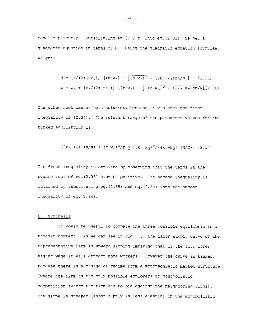
model explicitly. Substituting eq.(2.8.c) into eq.(2.31), we get a

quadratic equation in terms of H. Using the quadratic equation formulae,

we get:

H = [1/(2kj+k2)] (b-wo) - 2(b-wo) 2k+k 2 )bM/N ] (2.35)

w = wo + [k 1 /(2k 1 +k 2 )] [(b-wc) - (b-w)k2 -(2k +k 2 )bM/N,(2.36)

The other root cannot be a solution, because it violates the first

inequality of (2.34). The relevant range of the parameter values for the

kinked equilibrium is:

(2k 1+k 2 ) (M/N) < (b-wo)2/b < (3kj+k 2)2/(4kj+k 2) (M/N). (2.37)

The first inequality is obtained by observing that the terms in the

square root of eq.(2.35) must be positive. The second inequality is

obtained by substituting eq.(2.35) and eq.(2.36) into the second

inequality of eq.(2.34).

6. Synthesis

It would be useful to compare the three possible equilibria in a

broader context. As we can see in Fig. 3, the labor supply curve of the

representative firm is upward sloping implying that if the firm offer

higher wage it will attract more workers. However the curve is kinked,

because there is a change of regime from a monopsonistic market structure

(where the firm is the only possible employer) to monopolistic

competition (where the firm has to bid against the neighboring firms).

The slope is steeper (labor supply is less elastic) in the monopolistic

- 4' -

competition case than the monopsony case. The representative firm has to

pay more for the marginal worker in the former case, not because the

productivity of the marginal worker is higher in the former (in fact, it

is same as in the latter, i.e., b-c 2 (d)), but because, his alternative

wage is higher in the former case (i.e., w-c 1 (2H-d) > wo). The marginal

outlay curve represent the firm's marginal wage bill in order to have an

additional worker. As the supply curve is kinked, the marginal outlay

curve will have a jump at the kink. In fact, the size of the jump is

c 1'(d)d. Depending on where the marginal value product cuts through the

marginal outlay curve, we have three different cases of equilibrium. f

the curves intersect in the monopsony regime (point A in Fig. 3), we

will have the monopsony equilibrium, and so on. The kinked equilibrium

can occur only when there is a jump in the marginal outlay. In other

words, whenever the worker has to pay the signal acquiring cost, there is

a possibility of the kinked equilibrium. Thus, the kinked equilibrium

and its perverse comparative static will not occur if c 1' = 0

We plot the equilibrium wage with the size of the market in Fig.

4. If the size of the market (N) is smaller than N 1, the economy will

stay in the self-sufficient autonomy, where every worker gets wo. If N =

N 1 (= bM/[(2kj+k 2)(b-wo)2]), then the monopsony equilibrium will occur,

where the wage will be w, (= b - (kj+k 2 )(b-wo)) which is greater than wo.

If N 1 < N < N2 (= (4k1+k2 )bM/[(3kj+k2 )2 (b-wo)2]), then the economy stays

in the kinked equilibrium, where the wage decreases with the increase of

the market size. The kinked equilibrium occurs only in a limited range

of parameter values. The range will be small if M is small, k1 or k 2 is

large, and wo is large. If N > N 2 , then the economy will have the

monopolistic competition equilibrium where the wage increases

- 48 -

monotonically. However, the wage will be bounded by b. In other words,

the productivity increase through the better matching and specialization

will not exceed the technological upper limit.

III. Bargaining Equilibrium

1. Assumptions

Many assumptions in the bargaining model are very similar to

those in the signalling equilibrium model. Assumptions regarding the

workers are identical. Production technologies are the same. However,

we drop the assumption that firms cannot identify the characteristics of

workers. Thus, there is no need for signalling. The cost of mismatch,

which we shall denote c(t) where t is the distance between the worker and

the representative firm, is divided between the worker and the firm

through a negotiation. We shall assume that:

c(O) = 0 (3.1.a)

c'(t) > 0. (3.1.b)

For convenience, we assume that the cost will initially be borne by the

firm in the form of on-the-job-training.

The wage will be determined by the bargaining between workers and

firms. This wage determination rule drastically differs from the

signalling equilibrium where the wage is offered by the firm on a

take-it-or-leave-it basis. Since the firm can identify the workers, the

equilibrium wage w(t) will depend on the skill characteristic differences

between what the firm wants and what the workers have.

- 49 -

The key assumption that we adopt in this model is that all the

parties have equal bargaining power. More specifically, each party knows

exactly how much it will gain by having the employment contract, and the

bargaining outcome (i.e., wage) will be determined at the mid-point,

where the worker's surplus of having the employment contract over his

second best alternative is the same as the firm's marginal profit of

having the worker. Negotiation is costless, and collective bargaining by

workers or coalition formation by firms is not allowed. Since we shall

maintain the static framework, we also assume that no pair of agents will

miss a potentially beneficial bargaining opportunity.

Short run and long run are defined identically as in the case of

signalling equilibrium. In the short run, there is a fixed number of

firms, equally spaced. All firms earn zero profits in the long run.

Thus, the equilibrium distance and the number of firms will be

determined. Our major interest is, again, the long run symmetric Nash

bargaining equilibrium. By symmetry, we mean equal distance between any

two neighboring firms and identical wage equation for all firms.

The short run profit of the representative firm is:

p(d) = b[2Nd - M] - 2N [ fow(t)dt + d c(t)dt], (3.2)

where d is the market area of the representative firm. The only

difference between eq.(3.2) and eq.(2.5) is that the wage offer is a

function of the distance between the worker and the firm, whereas it is

constant in signalling model. This follows from the assumption that the

firm can discriminate workers.

The viability of any employment contracts will be determined by

- 50 -

whether the productivity of the employment is greater than the

reservation wage. The size of the difference between the productivity

and the reservation wage will not change the qualitative characteristics

of the equilibrium, since it does not affect the employment decision of

workers. However, the model will behave differently depending on the

number of potential employers the worker has. For example, if the worker

has two potential employers, then he can use one as a leverage for the

other in wage bargaining.

Monopsony case occurs then all workers in the economy has at most

one potential firm such that the marginal productivity of the roundabout

technology (net of training cost) is greater than the reservation wage.

If the former is smaller than the latter for all workers (b < wo), then

every agent will stay in the self-sufficient autonomy so that no labor

market can be established. This case will not be discussed further.

Competition case occurs when all workers have more than two potential

firms. Monopsony-competition case occurs when some workers have two

firms and the others have only one. Referring to Fig. 5, we can

identify the three cases. We will name them as follows:

1. Monopsony if b - c(H) < wo < b (3.3.a)

2. Monopsony-competition if b - c(2H) < wo < b - c(H) (3.3.b)

3. Competition if wo < b - c(2H). (3.3.c)

Of course, we will restate the conditions in terms of all exogenous

parameters later, as H is endogenous in the long run.

2. Monopsony case

- 51 -

In the monopsony case, some workers have one potential employer

while the others do not have any viable employment opportunity. Thus,

the latter will stay out out the labor market voluntarily. Thus, every

worker in the economy has at most one potential employer such that the

productivity of employment is greater than the reservation wage.

The equal bargaining power implies that:

b - c(t) - w(t) = w(t) - w., 0 < t < d, (3.4)

for the workers whose productivity is higher than the reservation wage.

The left hand side represents the firms marginal profit net of the wage

payment, and the right hand side is the worker's additional wage earned

by working for the firm rather than working for himself. From eq.(3.4)

and individual rationality, the bargaining equilibrium wage will be:

w(t) = [wo + b - c(t)] / 2, 0 < t < d. (3.5)

The market area will be determined by:

d = c~ (b-wo), (3.6)

since w(d) = w.. Let us assume that c(t) is linear, that is:

c(t) = kt. (3.7)

Then eq.(3.6) implies that:

- 52 -

d = (b-wo) / k. (3.8)

Imposing the zero profit condition, we get:

(b-wo)2 / b = 2kM / N. (3.9)

If the left hand side of eq.(3.9) is smaller than the right hand side,

then firms will earn negative profits. There will be no labor market

equilibrium in the long run, since the firm cannot fully recover its

fixed cost of the roundabout technology. On the other hand, if the left

hand side is larger, then more firms will enter so that situation becomes

either the monopsony-competition case or the competition case.

As we indicated in the monopsony case of the signalling

equilibrium there may be gaps between neighboring firms (i.e. some

workers will not seek a bargaining opportunity in the labor market).

Thus, the number of firms in the long-run is not unique. However, the

maximum number of the firms m* will be:

m= k / 2(b-wo). (3.10)

It appears that the equilibrium market area (eq.(3.8)) and the maximum

number of firms (eq.(3.10)) are independent of M and N, unlike in the

case of the signalling equilibrium. This is not case, because the extra

constraint (eq.(3.9)) must be satisfied. Just as the monopsony

equilibrium in the signalling model, the monopsony equilibrium in the

bargaining model can only occur on the knife edge value of parameter. If

we substitute (eq.(3.9)) into eq.(3.8) and eq.(3.10), then we get very

- 53 -

similar results as to the signalling equilibrium case.

The average wage of the workers in the economy will be:

W = wo + (b - wo) 2 / 4kH, (3.11.a)

which will be reduced to:

W = (b + 3wo) / 4, (3.11.b)

when there is no gap (d = H). It is clear that W > wo.

3. Competition case

The competition case occurs when every worker in the economy can

potentially work for at least two firms whose marginal product is higher

than the worker's reservation wage. We assume that the bargaining occurs

only among the three agents, that is, the representative worker and the

two firms which have the least and the second least training cost for the

worker. Since the theory of three person bargaining games has not been

developed fully, the choice of the threat point of the worker is not

evident. In the monopsony case, there are only two parties involved, and

their threat points are exogenous and known to the bargainers. Thus the

outcome is well defined with the equal bargaining power assumption..

However, in the competition case, the worker's threat point is the

outcome of the bargaining between the worker and the other firm, which in

turn, is the outcome of the bargaining with the first firm. This point

creates a non-trivial theoretical difficulty.

One plausible bargaining outcome in this case is7 :

- 54 -

w(t) = [b - c(t)]/2 + [b - c(2H - t)]/2. (3.12)

In this formulation, the worker's alternative wage is assumed to be the

highest possible wage in the negotiation with the other firm. Although

this specification seems to overstate the bargaining power of the worker,

it is compatible with our assumptions. To see this, notice the

difference of the bargaining positions between workers and firms in the

competition case. While the worker can only work for one firm, the firm

can hire many workers. Thus, the worker is not substitutable to the

firm, while the firm is substitutable to the worker. In other words, the

firm has only one potential bargaining opportunity with the worker. If

the worker does not accept the employment contract, then the firm loses

its production opportunity with the worker for ever. This is not case

for the worker. If one firm does not accept the employment contract,

then he has another chance with the other firm.

With the linearity of the training cost assumption, we get the

equilibrium wage function,

w(t) = b - kH, (3.13)

which, interestingly enough, is independent of t. There are two elements

in determining the wage of a worker. The worker who has a good match

with one firm can demand higher wage because he has high productivity.

However, the fact that he has a good match with one firm necessarily

implies that he has a poor match with other firms. Since he has poor

match with the other firm, his bargaining position will be weakened.

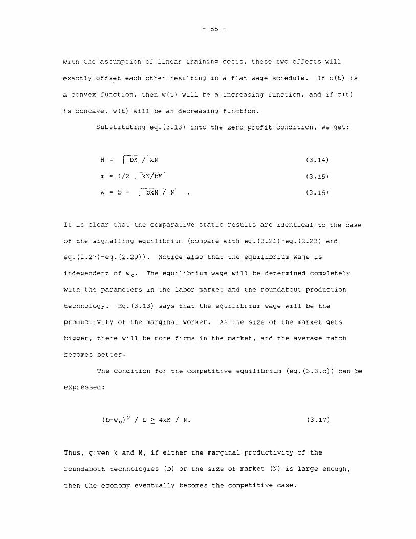
- 55 -

With the assumption of linear training costs, these two effects will

exactly offset each other resulting in a flat wage schedule. If c(t) is

a convex function, then w(t) will be a increasing function, and if c(t)

is concave, w(t) will be an decreasing function.

Substituting eq.(3.13) into the zero profit condition, we get:

H= bM kN (3.14)

m = 1/2 1 kN/bM (3.15)

w =b - ibkM / N . (3.16)

It is clear that the comparative static results are identical to the case

of the signalling equilibrium (compare with eq.(2.21)-eq.(2.23) and

eq.(2.27)-eq.(2.29)). Notice also that the equilibrium wage is

independent of wo. The equilibrium wage will be determined completely

with the parameters in the labor market and the roundabout production

technology. Eq.(3.13) says that the equilibrium wage will be the

productivity of the marginal worker. As the size of the market gets

bigger, there will be more firms in the market, and the average match

becomes better.

The condition for the competitive equilibrium (eq.(3.3.c)) can be

expressed:

(b-wo)2 / b > 4kM / N. (3.17)

Thus, given k and M, if either the marginal productivity of the

roundabout technologies (b) or the size of market (N) is large enough,

then the economy eventually becomes the competitive case.

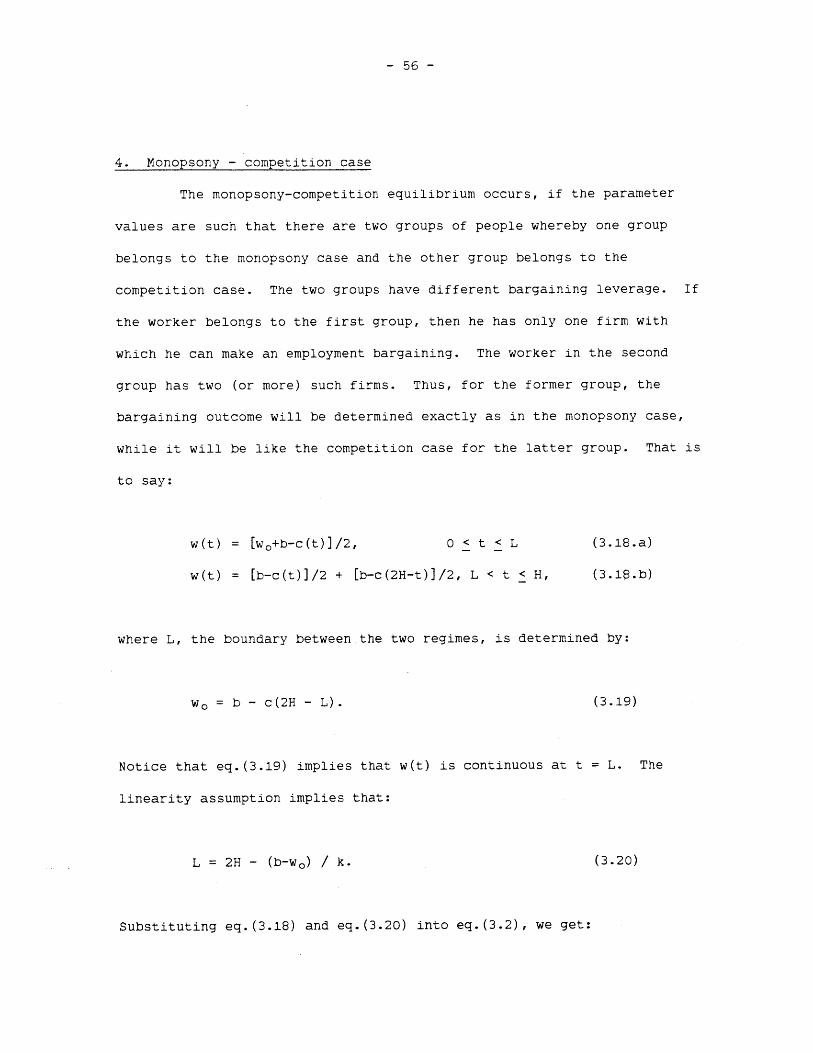
- 56 -

4. Monopsony - competition case

The monopsony-competition equilibrium occurs, if the parameter

values are such that there are two groups of people whereby one group

belongs to the monopsony case and the other group belongs to the

competition case. The two groups have different bargaining leverage. If

the worker belongs to the first group, then he has only one firm with

which he can make an employment bargaining. The worker in the second

group has two (or more) such firms. Thus, for the former group, the

bargaining outcome will be determined exactly as in the monopsony case,

while it will be like the competition case for the latter group. That is

to say:

w(t) = [wo+b-c(t)]/2, 0 < t < L (3.18.a)

w(t) = [b-c(t)]/2 + [b-c(2H-t)]/2, L < t < H, (3.16.b)

where L, the boundary between the two regimes, is determined by:

wo = b - c(2H - L). (3.19)

Notice that eq.(3.19) implies that w(t) is continuous at t = L. The

linearity assumption implies that:

L = 2H - (b-wo) / k. (3.20)

Substituting eq.(3.18) and eq.(3.20) into eq.(3.2), we get:

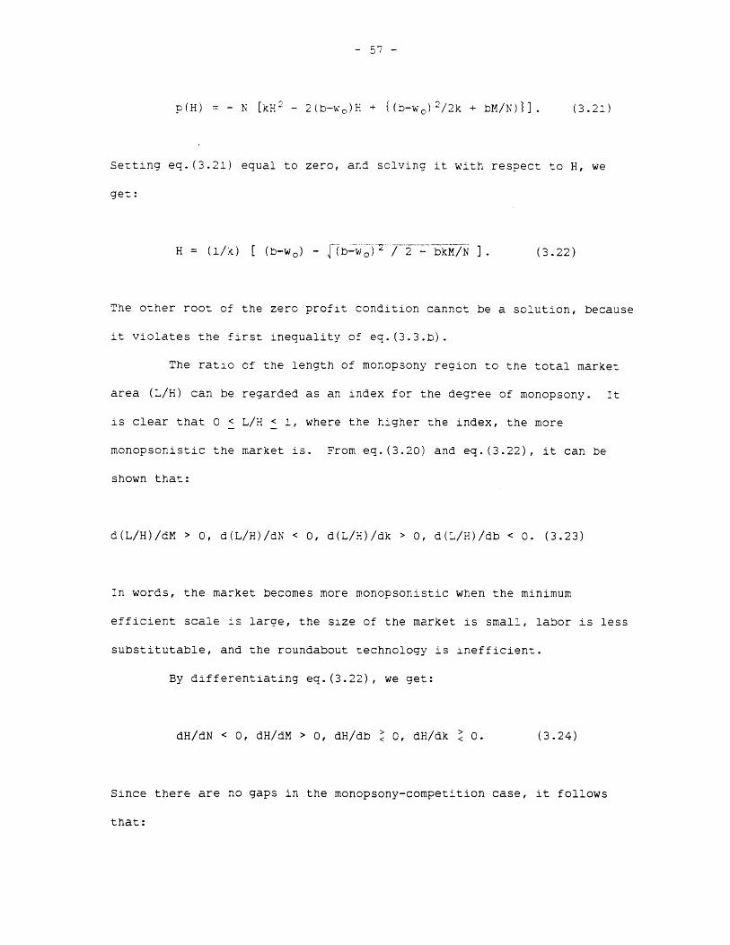
- 57 -

p(H) = - N [kH2 - 2(b-wo)H + {(b-w )2/2k + bM/N)}]. (3.21)

Setting eq.(3.21) equal to zero, and solving it with respect to H, we

get:

H = (1/k) ( (b-wo) - ib-w 2 - bkM/N ]. (3.22)

The other root of the zero profit condition cannot be a solution, because

it violates the first inequality of eq.(3.3.b).

The ratio of the length of monopsony region to the total market

area (L/H) can be regarded as an index for the degree of monopsony. It

is clear that 0 < L/H < 1, where the higher the index, the more

monopsonistic the market is. From eq.(3.20) and eq.(3.22), it can be

shown that:

d(L/H)/dM > 0, d(L/H)/dN < 0, d(L/H)/dk > 0, d(L/H)/db < 0. (3.23)

In words, the market becomes more monopsonistic when the minimum

efficient scale is large, the size of the market is small, labor is less

substitutable, and the roundabout technology is inefficient.

By differentiating eq.(3.22), we get:

dH/dN < 0, dH/dM > 0, dH/db > 0, dH/dk > 0. (3.24)

Since there are no gaps in the monopsony-competition case, it follows

that:

- 58 -

dm/dN > 0, dm/dM < 0, dm/db > 0, dm/db > 0. (3.25)

The equilibrium number of firms will be large if the size of the market

is large and if the minimum efficient scale M is small. The intuition

for these results is quite clear. It the size of the market is large

(i.e., the density of the market is high), the the firm does not have to

hire the workers whose skill characteristics are quite different from its

ideal one in order to recover the fixed cost generated by the minimum

efficient scale. By the same token, if the minimum efficient scale is

large, then the firm has to hire many workers whose skill characteristics

are not so ideal.

The effect of the change of marginal productivity is ambiguous.

If the economy is close to the monopsony case (i.e., L is close to H),

then the higher marginal productivity will increase output while the wage

function will not be affected significantly. Thus, firms are more

profitable. Consequently, more firms will enter the market. On the

contrary, if the economy is similar to the competition case (i.e., L is

close to zero), then the firm has to pay a higher wage, which is

determined by the new marginal worker, to most of the workers. Thus, the

increase in the wage bill would outweigh the increase of the

productivity. Firms will exit, because they yield negative profits.8 The

effect of the change of the training cost is also ambiguous. If the

economy is close to the monopsony case, then dH/dk > 0, and vice versa.

The intuition is roughly the same as the marginal productivity case.9

The average wage will be:

W = (b - kH) + (2kH - (b-wo))2 / 4kH,

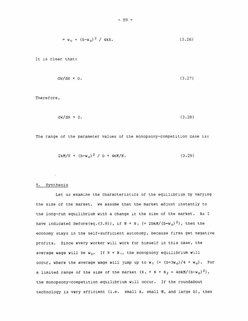
- 59 -

= wO + (b-wo)2 / 4kH. (3.26)

It is clear that:

dW/dH < 0. (3.27)

Therefore,

dW/dN > 0. (3.28)

The range of the parameter values of the monopsony-competition case is:

2kM/N < (b-wo)2 / b < 4kM/N. (3.29)

5. Synthesis

Let us examine the characteristics of the equilibrium by varying

the size of the market. We assume that the market adjust instantly to

the long-run equilibrium with a change in the size of the market. As I

have indicated before(eq.(3.9)), if N < N1 (= 2bkM/(b-wo) 2 ), then the

economy stays in the self-sufficient autonomy, because firms get negative

profits. Since every worker will work for himself in this case, the

average wage will be wo. If N = N 1 , the monopsony equilibrium will

occur, where the average wage will jump up to w 1 (= (b+3wo)/4 > wo). For

a limited range of the size of the market (N 1 < N < N 2 = 4bkM/(b-wo) 2 ),

the monopsony-competition equilibrium will occur. If the roundabout

technology is very efficient (i.e. small k, small M, and large b), then

- 60 -

the range where the monopsony-competition equilibrium occurs is small.

Although the effects of changing b and k are ambiguous in this

case, there is no perverse effect of the size of the market in the

bargaining equilibrium. The market area continually declines with the

increase of the size of the market (refer to Fig. 6). Similarly, the

average wage rises in the same range. The rise of the average wage can

be attributed to two factors. The first element is that the average

match gets better by having smaller market area (eq.(3.23)). The second

element, which is unique to the bargaining model, is that more and more

workers have better bargaining position, as their productivity with the

other firm exceeds the reservation wage.

One may wonder why the perverse effect of the kinked model of the

signalling equilibrium does not occur in the bargaining model. The

fundamental reason for the perverse effects of the kinked equilibrium is

that the labor supply is less elastic in the monopolistic competition

case than the monopsony case. This is counter-intuitive, since one would

associate competition with high elasticity. This is a peculiar result of

the original set-up of Salop [1979] in which the firm has to pay the

higher wage to all workers when the marginal worker has an alternative

firm to work for. Thus, there is a discontinuity in the wage function

between the monopsony and the monopolistic regime.

In the bargaining model, the change of regime happens in a more

gradual way. To see this, let us use Fig. 7 for illustration. If N =

N 1 , then the equilibrium distance will be H1, and the equilibrium wage

function will be line AC'. If N increases, then H decreases. Let us

choose N such that N 1 < N < N 2, then monopsony-competition equilibrium

will occur, and the equilibrium distance (H3) will lie between H 1 and H 2.

- 61 -

The wage function is now line BB'C. Workers between 0 and H 4 have only

one employment opportunity, while workers between H 4 and H 3 have two

opportunities. Thus their wage schedule is BB' rather than AB'. If N >

N 2, then H < H 2. Thus competition equilibrium occurs. Let us choose a

point H 5. The equilibrium wage schedule is flat in the competition case.

As N approaches infinity, the wage approaches b and H approaches zero.

IV. Conclusion.

We have developed two simple models in which labor is not

homogeneous, and the roundabout technology has increasing returns to

scale, in order to analyze the effects of labor specialization in a

modern economy. The major point is that in a highly concentrated modern

urban economy, the geographical proximity among workers and firms

facilitates a specialized labor market. Since specialization reduces the

training cost (or the loss of the productivity due to the mismatch

between workers and firms), the average productivity increases with the

size of the market except the kinked equilibrium case in the signalling

model where the average productivity decreases with the size of the

market.

The perverse effect of the kinked equilibrium of the signalling

model will not occur in the bargaining model, because the transition from

the monopsony regime to the monopolistic competition region is smooth in

the latter. Even in the signalling model, if the market size is big

enough, then the economy will have the monopolistic competition

equilibrium in which the average productivity will increase with the size

of the market. In that regime, the wage will be higher, if the

- 62 -

roundabout technology has high marginal productivity, low minimum

efficient scale, and low training cost.

- 63 -

f irm i(the representative firm)

offering w

firm joffering w

0

t --- )h----- 2H - t ) o

Figure 1. The Representative Firm and the Workers Close to It

Monopsony Case

Yinked Case

Monop olis ticCompetition Case

0 H

Figure 2. Three Possible Cases in Signalling Model

2H

(t) w-c(2H-t)

- 64 -

w

b

Monopolisticcompetitionequilibrium

Kinkedequilibrium

Monopsonyequilibrium

w0

marginal value product

b - c2 (d)

marginal outlay

w + 2c1 '(d)d + c (d)o 1 1

labor supply

monopsonyregime

--- monopolistic competition

regime

Figure 3. Three Possible Equilibria in Signalling Model

0

- 65 -

w

b

w= b - (k + k2 )(b - w )

(2k 1+k2)(3k +k 2)b - 12 (b-w )

4kI+k2 0

= 2

( 1 bM (4k1+k2) bM1 2k +k 2 2 2 2

1 2 (b-w ) (3k +k2) (b-w0)

Figure 4. Size of the Market and Equilibrium Wagein Signalling Model

N

1. Monopsony

2. Monopsony-

Competition

3. Competition

0

Figure 5. Three Possible Cases in Bargaining Model

- 66 -

H

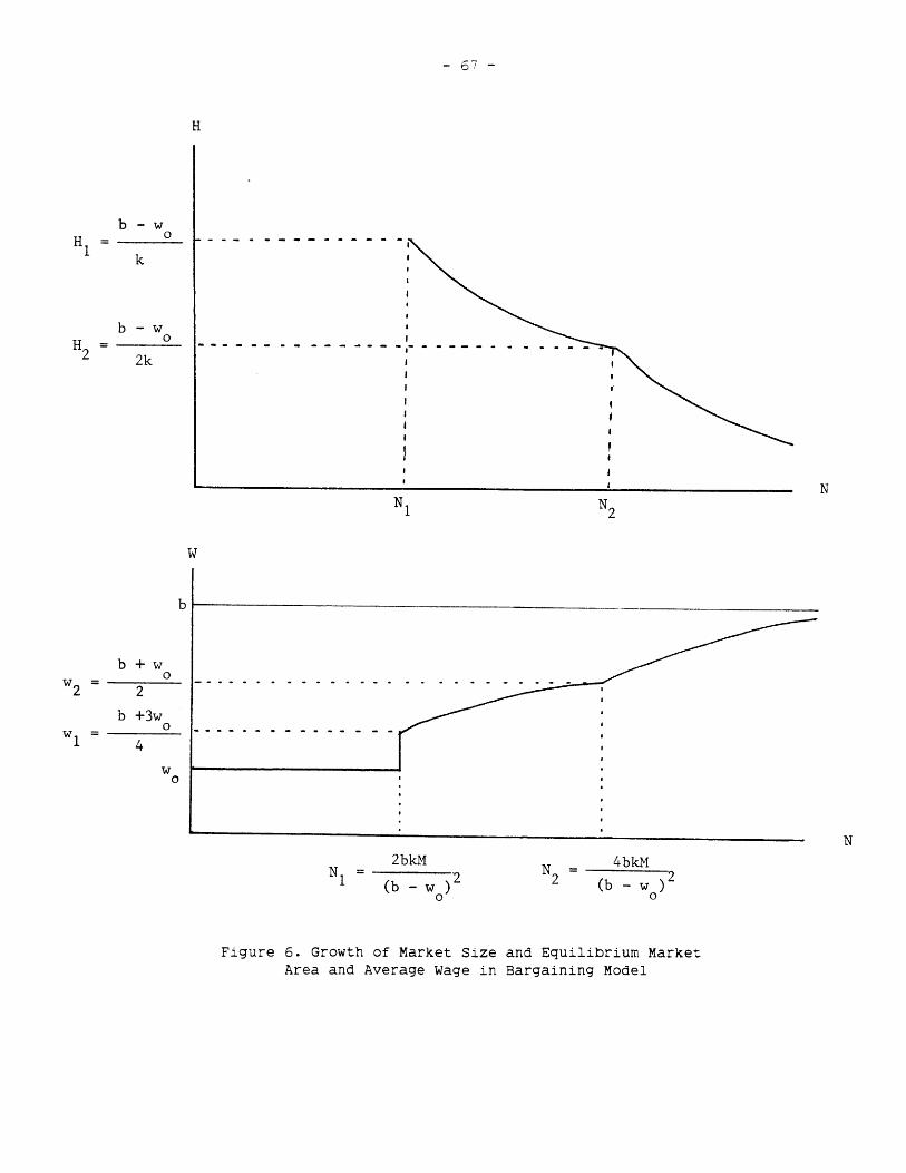
- 67 -

H

b - wH = 01 k

b - wH =202 2k

N1

W

b

b + w0

w 2 2

b +3w0

4

w0

NN2

2bkMN = (b - w ) 2

N

N - 4bkM2 (b - w )

Figure 6. Growth of Market Size and Equilibrium MarketArea and Average Wage in Bargaining Model

wi

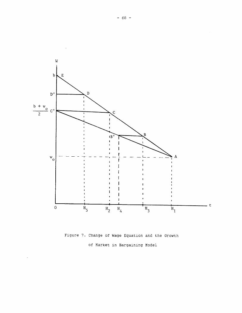
- 68 -

w

b E

D' D

b + w0 ,

2 C

B',

I 0

t . tH5 H2 H4 H3 1H

Figure 7. Change of Wage Equation and the Growth

of Market in Bargaining Model

69 -

Footnotes

1. This model has a similar basic structure with Salop'sL1979]. Themajor differences are; first, the focus is the labor marketrather than the output market; second, sellers as well asbuyers must incur some costs if the characteristic of the buyerdoes not match exactly with the characteristic of the seller.Namely, c 2 (t) = 0 in Salop.

2. The condition that c 1">0 is more than necessary. This can be relaxedfurther in many cases.

3. There has been a criticism for the use of Nash equilibrium concept inthis type of circle model (Hart[1983]). The argument is thatthe Nash assumption is not very convincing, since each agentinteracts only with two neighboring firms directly. It ispossible to get around this criticism by modifying the modelinto two dimensions such that there are many neighboring firmsfor each firm. Consider the following short run set-up. Thereare m firm indexed 1 to m. There is a continuum of workersindexed (i,j,t) with aggregate size N. Worker (i,j,t) can workonly firm i or j. All ordered pairs (i,j) have equalpopulation weight. For each (i,j) t is uniformly distributedon the unit interval. The behavior of the worker (i,j,t) isidentical to eq.(2.7). It turns out that the mathematics ofthis set-up is identical to the circle set-up of the text. Wewill stick to the circle set-up because of its intuitiveappeal.

4. Notice that we impose symmetry after differentiation.

5. One can easily verify that the second order condition is alsosatisfied.

6. Instead of using the wage offer, one can use average net wage toyield the same comparative static results.

7. It is interesting that some plausible wage functions have seriousdefects. One would think that the following is a reasonablewage function:

w(t) = (b-c(t))/2 + ;(2H-t)/2, (A.1)

where w(.) = w(.) at equilibrium. The problem of thisformulation is that (2H-t)/2 is not a credible threat point,because w(2H-t) > b - c(2H-t) if t < H. In other words, the

- 70 -

other firm Will not engage in the employment contract which

yield negative return. The other plausible wage function is:

w(t) = (b-c(t))/2 + [(wo+b-c(2H-t))/2]/2. (A.2)

This can not be an equilibrium wage function, because it is not

stable at the neighborhood of the marginal workers where the

wage is lower than the marginal productivity with the other

neighboring firm. Let us choose the worker at the midpoint

(t = H) for illustration. Since w(H) < b-c(H), he can make a

mutually beneficial employment contract with the other firmwith the wage higher that w(H). After he gets the higher wage,he can open a new employment negotiation with the original firmand demand even higher wage.

8. For example, let w. = 0. Then it can be shown that:

dH/db < 0, if 2kM/N < b < (f2+1)kM/N (A.3.a)dH/db > 0, if (.2+1)kM/N < 4kM/N. (A.3.b)

9. It can be shown that:

dH/dk > 0, if 2kM/N < (b-w0 )2/b < [(3+2{2)/(t2+1)]

kM/N (A.4.a)dH/dk < 0, if [(3+22)/(d2+1)] kM/N < (b-wo) 2/b <4kM/N. (A.4.b)

- 71 -

CHAPTER III

Labor Specialization Decisions and the Extent of the Market

I. Introduction

In this chapter, we analyze an extension of the model presented

in the previous chapter. Namely, we shall allow workers to choose their

human capital. In the two models of the previous chapter, workers' skill

characteristics are exogenously given. Since we shall consider the

extension of the bargaining model only, the "previous model" refers to

the bargaining model in Chapter II.

The human capital investment decision of the worker has two

distinct dimensions. First, he decides on how much he will accumulate

his human capital on certain skill characteristics. The usual

terminology of "skilled labor" and "unskilled labor" stems from this

consideration. However, the treatment of human capital as a scalar is

not very satisfactory, once one recognizes the heterogeneity of labor.

For example, a computer programmer would be regarded as a "skilled labor"

for data processing industry while he is a "unskilled labor" for

construction industry. The second dimension the worker decides on is the

breadth of his human capital. A computer programmer may train himself

for a wide range of software and hardware. Alternatively, he may learn

only a specific programming language on a specific hardware. We shall

call them intensive and extensive human capital, respectively.

In the modern economy where labor demand is also highly

- 72 -

specialized, extensive human capital is as important as intensive human

capital, because there is an important trade-off between them. Although

a specialist will be more productive than a generalist in a limited range

of tasks which require the specialist's skill, the probability of getting

such a good-matching job will be smaller for the specialist.

To characterize the worker's human capital in this way has a

number of advantages over the approach in which it is characterized by a

vector of skills. First, we can parameterize it completely in two

variables (intensive human capital and extensive human capital) rather

than a vector with a higher dimension. Second, it is not very clear how

one defines a wide range of skills in a finite vector. Third, the former

approach can incorporate the natural difference of human potentials in a

more reasonable way. This point will be made clear when we discuss the

structure of the model.

With the given cost of acquiring human capital, a worker may

invest more intensively and less extensively, or vice versa. We say that

worker A is more specialized than worker B, if worker A has more

intensive and less extensive human capital than worker B. Sometimes we

refer the former a specialist, and the latter a generalist. In our

model, the choice of skills to specialize (say, the choice of occupation)

is determined by the worker's potential ability endowed with his birth.

In this chapter, we will analyze the relationship between the

worker's human capital investment decision and the size of the market by

using a similar model described in the previous chapter. The major

difference between the model in this chapter and in the previous one is

that workers can choose the marginal productivity of the ideal worker in

the production technology (b) and the loss of productivity due to the

- 73 -

mismatch between the job and the worker (c(t)). We shall only focus our

attention on the bargaining model because it has the simpler analytical

structure than the signalling model.

As in the previous model, three cases can be distinguished based

on the number of viable jobs a worker has. A viable job for a worker is

the job which pays higher wage than the worker's reservation wage. The

case in which all workers in the economy have at least two viable jobs

will be called competition case. If all workers have at most one job

opportunity, then it is called monopsony case. The third case in which

some of the workers have only one viable job opportunity whereas the

others have two will be called monopsony-competition case. Notice that

the competition case occurs when every worker has human capital general

enough to work for at least two firms which require different skill

characteristics.

In section II, assumptions of the model will be described. Many

assumptions are the same as in the previous model. Thus, only the

assumptions different from those of the previous one will be spelled out

in detail. In section III, the competition case will be analyzed. The

monopsony case will be analyzed in section IV. The monopsony-competition

case will be analyzed in section V. Conclusions will be given in section

VI.

II. Assumptions

Consider a closed economy of a continuum of workers-cum-consumers

with aggregate size N. Workers are indexed on a circle of a unit length

with uniform density. Since the circle has the unit length, the density

- 74 -

is also N. The index represents the worker's potential ability. The

same index represented the worker's actual skill characteristic rather

than his potential in the previous model. As in the previous chapter, we

will call the index location and the difference between two indices

distance.

Since we assume that the worker knows his potential ability, he

will invest in his human capital around it. It acts as an anchor for his

human capital investment decision. In this model, the worker's actual

skill characteristic is determined by his human capital investment as

well as his potential ability. Notice, however, that human capital

investment does not change the worker's index. Thus, we can identify the

worker with his potential ability, even after his human capital

accumulation is finished. In other words, even though we allow worker to

choose his human capital, we do not allow them to choose their best skill

characteristics. Thus, the choice of skill characteristic (say,

occupation) is excluded in the model. For example, a computer programmer

is born with the potential ability to be a computer programmer, and he

knows that his potential ability is strongest in computer programming.

Thus, he will be a computer programmer. The only decisions he makes are:

1) How much he will invest in computer programming (say, get a Master's

degree or go to a technical school); and 2) How wide he will train

himself (e.g., only learn one programming language in one machine or

learn a variety of different languages and machines).

In particular, we shall assume that the representative worker

chooses two variables (b, K) to maximize his lifetime expected utility.

We assume risk neutrality of workers. Since our model is a static one,

it follows that the worker maximizes the expected wage net of the cost of

- 75 -

acquiring the human capital. We normalize the location of the

representative worker to the origin (zero) without loss of generality.

We shall call the two variables intensive human capital and extensive

human capital. The variable b (intensive human capital) represents the

marginal productivity of the worker when he works for the firm which

requires the same skill characteristic. In the previous model, b was

parameterized as the marginal productivity of the "ideal" worker to a

given firm, and was given exogenously. In this model, we shall treat b

as a worker's decision variable.

The worker also makes a decision on K (extensive human capital).

Generally, the more extensive human capital, the lower the expected cost

of mismatch between the job and the worker, given the intensive human

capital and labor demand. Specifically, we assume that the cost of

mismatch between the job and the worker is assume to be:

c(t) = t/K (2.1)

where t is the distance between the worker and the firm. Notice that the

cost of mismatch is independent of b. One can view the above mismatch

function as a reparameterization of the linear cost function of the

mismatch (eq.(3.7) in Chapter II). From the viewpoint of the previous

model, the worker is now allowed to choose the marginal productivity of

the roundabout technology (b) and the inverse of the slope of the linear

mismatch cost function (k = 1/K).

Although the model is presented in a static setting, one can

conceptually divide it into two stages. In the first stage, workers make

their human capital investment decisions (i.e., choose b and K). They

- 76 -

know the aggregate size of the market and the wage determination rules.

Thus, given b and K, they can calculate their expected wage and the cost

of acquiring human capital. We impose the symmetry that every worker

invests to the same level of b and K. In the second stage, the same

decision process in chapter II will be replicated. Firms will be

established, and they choose technologies (location). Given the location

of firms, workers make decisions whether to work or not, and if they

decide to work, they will choose the firm which they will work for. We

impose another kind of symmetry that all firms have same wage function,

and that the distance between any two neighboring firms are identical.

Equilibrium can only be realized when all firms get zero profits.

The parameters (b,K) are choice variables for the workers rather

than exogenous parameters. However, since we shall assume that workers

make human capital investment decisions before entering the labor market,

and that we restrict ourselves to the case where all workers have same

(b,K), firms will make production decision as if those are exogenous

parameters. Thus, the results of the previous model can be carried over

directly to the model in this chapter.

Firms (or plants) are assumed to produce homogeneous output,

which are sold in a competitive market. The price of output is

normalized to one. The firm's technology is defined by the minimum

efficient scale (M), which is exogenous and same for all firms, and its

ideal skill characteristic. The firm is also indexed on the unit circle,

where the index represents the its ideal skill characteristic. The

firm's ideal skill characteristic is the characteristic of the worker who

has the highest marginal productivity with the firm given the same

intensive human capital.

- 77 -

For the purpose of illustration, let us consider the computer

software industry. Firms produce homogeneous output called software.

One firm produces software by using one programming language. Other

firms produce same product by using different languages. Thus, they want

to hire workers who are good at the other kind of languages. If a firm

hires a worker who is not good at the language the firm uses, then the

cost of mismatching must incur in order to train the worker.

The production function of the representative firm is given by:

Y = C , if X < M'/b (2.2.a)

bX - M', if X > M'/b (2.2.b)

where

X = N 1 (1 - t/K) dt. (2.2.c)

Y denotes the output, X denotes the normalized input, M* denotes the

minimum efficient scale (which is given exogenously and same for all

firms), t denotes the distance between the firm and the workers, and the

integral is taken over the market area of the firm. This production

function is same as in the previous model except that the minimum

efficient scale is reparameterized to:

M* = bM. (2.3)

We assume that the cost of acquiring human capital g(b,K) is

assumed to be convex in b and K. Namely,

9b > 0, gK > 0 (2. 4. a)

- 78 -

gbb > 0, gKK > 0, gbK > 0 (2.4.b)

9bK gbbgKK < 0, (2.4.c)

where the subscripts refer to partial derivatives. The first set of

assumptions refer that the cost of acquiring human capital is an

increasing function of the level of both intensive and extensive human

capital. The second set of assumptions say that the marginal costs are

also increasing functions. The third assumption insures that the Hessian

of g(b,K) is negative definite. .

Workers and firms know exactly how much they will gain by having

employment contracts, and the wage will be determined at the mid-point

through bargaining between the worker and the firm, where the worker's

surplus of having the employment contract over his second best

alternative is same as the firm's marginal profit of having the worker.

Negotiation is costless, and collective bargaining is not allowed. Since

the model is static, we also assume that no pair of agents will miss a

potentially beneficial bargaining opportunity.

We will limit our analysis to the long run symmetric Nash

bargaining equilibrium. Long run is defined same as in the previous

model. All firms get zero profit and cost of relocating (adopting a new

technology) is zero. By symmetry we mean that: 1) All workers have same

(b,K); 2) The wage functions are identical for all firms; and 3) Firms

are equally spaced on the circle. The symmetry assumption is very

powerful despite its simplicity. It reduces the number of equilibria to

one except the monopsony case where there may be gaps between firms'

market areas. It is also a plausible assumption given that all workers

and firms have symmetric endowments.

- 79 -

The workers are assumed to have perfect information about the

size of the market and the wage determination rule so that they can

calculate the wage distribution function and the equilibrium distance

(2H) given (b,K). The actual wage is a random variable, however, since

the location of the firms is taken to be random. Although the worker

does not know the actual location of the firms, he knows the probability

distribution of the location. We assume that the probability density

function is uniform on the domain of [-H, H]. The support of the

probability density function shrinks as the number of firms in the market

increases. Roughly speaking, therefore, the location of the firm is more

predictable and the average distance between workers and firms is shorter

when there are more firms in the market. The reduction of uncertainty

does not play a role in this chapter because of the risk neutrality

assumption. Workers' choices of (b,K), in turn, determine the

equilibrium distance (2H) and the wage equation (w(t)) through the firms'

profit maximization condition and the zero profit condition as described

in chapter II.

III. Competition Case

As in chapter II, the competition case occurs when all workers in

the economy have at least two firms to work for. This condition for the

existence of the competition case implies that:

b - 2H/K > wo. (3.1)

We assume that a worker bargains only with the two firms which have the

- 80 -

two highest marginal productivities with the worker, and that the

worker's alternative wage is the highest possible wage in the negotiation

with the other firm (see Footnote 7 in chapter II for further

explanations).

With the linear mismatch cost function, the long run equilibrium

wage and equilibrium distance between any two neighboring firms are given

by (refer eq. (3.13) and eq. (3.14)in chapter II):

w(t) = b - H/K (3.2.a)

H = eK 1/2 (3.2.b),

where e = (M*I/N) 1/2 Since the wage is independent of the location of

firms, the expected wage net of the human capital cost (W) of the

representative worker is:

W = b - H/K - g(b,K). (3.3)

Excluding the possibilities of corner solutions, we get the two first

order conditions for the worker's expected net wage maximization problem

by differentiating eq.(3.3) with respect to b and K:

Wb = 1 - gb = 0 (3.4.a)

WK = HK-2 ~ 9K =0 (3.4.b)

It can be easily verified that the second order conditions are satisfied

by the assumptions of eq.(2.4):

- 81 -

Wbb = -gbb < 0 (3.5.a)

WKK = -2HK~ 3 - gKK < 0 (3.5.b)

WbK - WbbWKK = gbK - gbbgKK - 2HK- 3 gbb < 0. (3.5.c)

By substituting eq.(3.2.b) into eq.(3.4.b), the equilibrium conditions

can be re-written:

gb = 1 (3.6.a)

gK = eK-3/2 (3.6.b)

where all the variables are evaluated at the equilibrium. Notice that

the equilibrium conditions can be characterized by single parameter e.

In order to obtain comparative static results, let us consider a

small change in e. Taking total differentials, we get:

gbbdb + gbKdK = 0 (3.7.a)

3/2eK-5 1 2dK + gKKdK + gdb = K-3/2de (3.7.b)

Solving eq.(3.7.a) in terms of db, and substituting it into eq.(3.7.b),

it can be verified that:

dK K-3/2-- =-------------------------------------- > 0. (3.8)

de (3/2)/eK-5 2 _ (9bK- gbbgKK) / 9bb

From eq.(3.7.a) and eq.(3.8),

db/de = -(gbK/gbb) dK/de < 0. *39)

- 82 -

Then, it is straightforward to see:

dK/dN < 0, dK/dM* > 0 (3.10.a)

db/dN > 0, db/dM* < 0. (3.10.b)

Since the equilibrium number of firms in the market is (refer eq.(3.15)

in chapter II),

m = (1/2) e-2K-1/ 2, (3.11)

it is easy to see that:

dm/de = -(1/2)e- 2K-1 /2 _ (1/4)e-1K-3/ 2 dK/de < 0. (3.12)

Thus, it is clear that:

dm/dN > 0, dm/dM' < 0. (3.13)

In words, the equilibrium human capital of the representative worker will

be more specialized if the size of the market is larger and if the

minimum efficient scale is smaller. Also, there are more firms in the

market, when the size of the market is larger and the minimum efficient

scale is smaller.

It will be useful to think through why workers and firms are more

specialized in a larger market. First of all, given the characteristics

of the labor pool (b and K), there are more firms in a larger market

(eq.(3.11)). If the size of the market increases, there are more workers

- 83 -

whose marginal productivity is greater than the going wage. Thus, firms

will get positive profits, and new firms will enter.

If there are more firms in the market, the support of the

probability density function will shrink. Loosely speaking, it implies

that the probability of having a good-matching job increases. The

importance of extensive human capital declines relative to intensive

human capital. Therefore, workers will be more specialized. More

specialization implies higher b and lower K. This feedback effect

further increases the number of firms (eq.(3.ll)).

IV. Monopsony Case

In the monopsony case, all workers have at most one viable job

opportunity in which the worker gets higher wage than the reservation

wage. Since some workers will stay out of the market in the monopsony

case, the following condition must be satisfied for the workers who are

exactly in middle of any neighboring firms:

b - H/K < wo.. . (4.1)

Given b and K, the expected net wage for this case is determined by

(refer eq.(3.11) in chapter II):

W = wo + (b - wo) 2K / 4H - g(b,K), (4.2)

where H is any arbitrary positive real number satisfying eq.(4.1).

In order to get the first order conditions, we differentiate

- 84 -

eq.(4.2) by b and K:

Wb = (b - wo)K/2H - gb = 0 (4.3.a)

WK = (b - wo) 2/4H - gK = 0. (4.3.b)

The second order conditions in the monopsony case are slightly different

from those of the competition case (eq.(3.5)). They are:

K/2H - gbb 0 (4.4.a)

- gKK < 0 (4.4.b)

[(b-wo)/2H - gbK]2 + (K/2H - gbb) 9KK K 0 (4.4.c)

The convexity assumption of the human capital acquiring cost (eq.(2.4))

is not sufficient for eq.(4.4.a) and eq.(4.4.c) to be satisfied. In

order to satisfy eq.(4.4.a), a stronger condition is needed than gbb> 0.

Using the first order equilibrium conditions (eq.(4.3)), eq.(4.4.a) can

be re-written as:

gbb > g / 2 gw. (4.3.a')

Eq.(4.4.c) is more difficult to interpret. It is clear that the second

order term in eq.(4.4.c) is negative if eq.(4.3.a) is satisfied. By

using eq.(4.3.a), the first term of eq.(4.4.c) can be written as:

(b-wo)/2H - gbK = ge/K - gbK. (4.5)

It is not clear whether eq.(4.5) is positive or negative. The first term

- 85 -

in the right hand side of eq.(4.5) reflects the marginal cost of

acquiring intensive human capital averaged out by extensive human

capital. The second term reflects the marginal cost rather than the

average with respect to extensive human capital. Nonetheless, we shall

assume that eq. (4.4) be satisfied in the monopsony case and in the

monopsony-competition case, since workers take H exogenous in the latter

case also.

In the long run, the zero profit condition must be satisfied.

This condition does not determine H as in the cases of competition and

monopsony-competition. Instead, it gives an additional constraint on

(b,K):

(b-wo)2 = 2M' / KN. (4.6)

Thus, equilibrium b and K are overdetermined in the monopsony case,

because there are three equations to determine the two endogenous

equilibrium variables. Suppose that we determine the values of b and K

from eq.(4.3), and that we substitute them into eq.(4.6). If the left

hand side of eq.(4.6) is smaller than the right hand side, then firms

yield negative profits. Thus, there will be no monopsony equilibrium in

the long run, since the firms cannot fully recover the fixed cost of the

roundabout technology. On the other hand, if the reverse is true, then

more firms will enter the market. It will reduce H so that the

situations becomes either the monopsony-competition case or the

competition case.

Put differently, the monopsony equilibrium is on the knife-edge

in parameters (wo, M*, and N). Unless the parameters are such that there

- 86 -

exist b and K satisfying the three equilibrium conditions, the monopsony

equilibrium will not occur. The comparative static exercise cannot be

performed, because one cannot change one parameter values holding others

constant. If only one parameter is changed from an equilibrium, then the

economy can no longer be at an equilibrium, because not all the

equilibrium conditions can be satisfied any longer.

Notice that H is not determined by the equilibrium conditions.

The only restriction regarding to H is the inequality constraint of

eq.(4.1). Thus, there are infinite number of H's which satisfy the

constraint. If the equation is satisfied by the equality, then there are

no gaps between the market areas of any two neighboring firms. This

special case can be regarded as a limiting case of the

monopsony-competition case, which will be analyzed in the next section.

V. Monopsony-Competition Case

The monopsony-competition case occurs when some workers in the

economy have two viable jobs whereas the others have only one. This

implies that the productivity of the marginal worker who is at the

boundary of the firm's market area is greater than the reservation wage,

and that the productivity of the ideal worker of the neighboring firm at

the representative firm is lower than the reservation wage. Namely,

b - 2H/K < wo < b - H/K. (5.1)

As shown in chapter II, the expected net wage of the worker in the

monopsony-competition case has the same functional form as in the

- 87 -

monopsony case (refer eq.(3.26) in chapter II):

W = w 0 + (b - w0 )2K / 4H - g(b,K), (5.2)

Unlike the monopsony case, however, H is determined endogenously (refer

eq.(3.22) in chapter II):

H = K [ (b-wo) - {(b-w 0 ) 2 / 2 - e 2 /K 1/ 2 ]. (5.3)

Differentiating eq.(5.2), we get the first order conditions for

the worker's expected net wage maximization problem:

Wb = (b - wO)K/2H - gb = 0 (5.4.a)

WK = (b - wo) 2/4H - gK = 0. (5.4.b)

The second order conditions are assumed to be satisfied as in the

monopsony case. Since the worker is assumed to take H given, the first

order conditions are identical to those of the monopsony case even though

H is determined endogenously. However, eq.(5.3) constitutes an

equilibrium condition as well as eq.(5.4) to determine the equilibrium

(b,K,H).

Let us denote the right hand side of eq.(5.3) as:

H = h(b,K,e). (5.3')

By using the existence condition of the monopsony-competition case

(eq.(5.1) or eq.(3.29) in chapter II), it can be shown that:

- 88 -

hb < 0 , h K > 0, he > 0. (5.5)

Intuitively speaking, if the average productivity of workers (b)

increases ceteris paribus, then the firm's profit increases because the

firm gets a half of the productivity increases by the equal bargaining

power assumption. Higher profits induce the entry of new firms. If the

labor pool is more substitutable (higher K), the labor market becomes

more competitive. Then the area of the competitive regime relative to

the firm's market area will increase. This will raise the firm's average

wage bill. Profits will decline, and firms will exit. If the size of

the market (N) increases or if the fixed cost element (M ) decreases,

firms will get higher profit, which leads to the entry of new firms.

In order to examine the comparative static results, we take total

differentials of the equilibrium conditions:

K b-we (b-wo)K

(-- - gbb) db + (---- - gbK) dK - -------- dH = 0 (5.6.a)2H 2H 2H 2

b-wa (b-w 0 ) 2

(---- - 9bK) db ~ 9KK dK ---------- dH = 0 (5.6.b)2H 4H 2

- hb db -hK dK + dH =he de (5.6.c)

It is impossible to come up with an unambiguous result by applying

Cramer's rule to eq.(5.6), because: 1) the sign of the expression

(b-wo)/2H - gbK (eq.(4.5)), is not determined a priori, and 2) some of

the terms would have ambiguous signs even if the sign of that expression

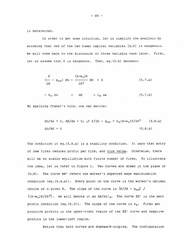
- 89 -

is determined.

In order to get some intuition, let us simplify the analysis by

assuming that one of the two human capital variables (b,K) is exogenous.

We will come back to the discussion of three variable case later. First,

let us assume that K is exogenous. Then, eq.(5.6) becomes:

K (b-wo)K

(-- - gbb) db - -------- dH = 0 (5.7.a)2H 2H2

- hb db + dH =he de (5.7.b)

By applying Cramer's rule, one can derive:

db/de < 0, dH/de > 0; if K/2H - gbb < hb(b-wo)K/2H 2 (5.8.a)

db/dH < 0 (5.8.b)

The condition in eq.(5.8.a) is a stability condition. It says that entry

of new firms reduces profit per firm, and vice versa. Otherwise, there

will be no stable equilibrium with finite number of firms. To illustrate

the idea, let us refer to Figure 1. Two curves are drawn in the plane of

(b,H). The curve WW' refers the worker's expected wage maximization

condition (eq.(5.4.a)). Every point on the curve is the worker's optimal

choice of b given H. The slope of the curve is {K/2H - gbb} /

{(b-wo)K/2H 2}. We will denote it as dH/dblw. The curve ZZ' is the zero

profit condition (eq.(5.3)). The slope of the curve is hb. Firms get

positive profits in the upper-right region of the ZZ' curve and negative

profits in the lower-left region.

Notice that both curves are downward-sloping. The configuration

- 90 -

in Figure 1 (i.e., dH/dbtw < hb) shows an stable equilibrium. The exact

dynamic structure will be spelled out later. Suppose the size of the

market (N) increases. This means e declines. Then, the ZZ' curve will

shift down, since he > 0. The initial equilibrium point A is now in the

region of positive profits. Thus, firms will enter. The entry will

reduce H. Workers invest more in b to take advantage of the reduction of

H. Although profit will increase by the increase of the productivity of

workers, it will be dominated by the decrease of profits due to the

larger number of firms. Since profit will decrease with more entry, the

economy will reach a new equilibrium point B where firms get zero

profits.

If the slope of the ZZ' curve is steeper than that of the WW'

curve, on the contrary, then the system is not stable. For example, if N

increases, then firms get positive profit. More firms will enter.

Workers will invest more in b. The increase of profit due to the higher

productivity of the workers will be stronger than the dilution of profits

due to the new entry. Thus, more firms will enter and the process goes

on without stopping.

Notice that we have adopted a particular dynamic structure,

namely, we assumed that the entry and exit of firms is the key element of

adjustment. If the size of the market or the minimum efficient scale

changes, then profits will rise or fall holding (b,K) constant. Since

non-zero profits will induce entry or exit of firms, H will vary. As H

varies, workers make a new choice of (b,K). With different (b,K) H will

vary, and the process keeps going until it reachs another equilibrium.

Let us turn to the case where b is taken exogenous and (K,H) are

endogenous. Then, it is straightforward to show that:

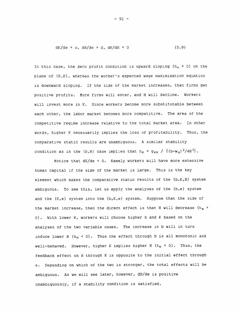
- 91 -

dK/de < o, dH/de > 0, dK/dH < 0 (5.9)

In this case, the zero profit condition is upward sloping (hk > 0) on the

plane of (K,H), whereas the worker's expected wage maximization equation

is downward sloping. If the size of the market increases, then firms get

positive profits. More firms will enter, and H will decline. Workers

will invest more in K. Since workers become more substitutable between

each other, the labor market becomes more competitive. The area of the

competitive regime increase relative to the total market area. In other

words, higher K necessarily implies the loss of profitability. Thus, the

comparative static results are unambiguous. A similar stability

condition as in the (b,H) case implies that hK < 9KK / {(b-w 0 )2/4H 2}

Notice that dK/de < 0. Namely workers will have more extensive

human capital if the size of the market is large. This is the key

element which makes the comparative static results of the (b,K,H) system

ambiguous. To see this, let us apply the analyses of the (b,e) system

and the (K,e) system into the (b,K,e) system. Suppose that the size of

the market increase, then the direct effect is that H will decrease (he >

0). With lower H, workers will choose higher b and K based on the

analyses of the two variable cases. The increase in b will in turn

induce lower H (hK < 0). Thus the effect through b is all monotonic and

well-behaved. However, higher K implies higher H (hK > 0). Thus, the

feedback effect on H through K is opposite to the initial effect through

e. Depending on which of the two is stronger, the total effects will be

ambiguous. As we will see later, however, dH/de is positive

unambiguously, if a stability condition is satisfied.

- 92 -

Let us come back to the original system in which b and K are both

endogenous as well as H. One can re-write the equilibrium equations into

a more manageable form by noticing that the worker makes a choice of

(b,K) only on the basis of H. There are no direct effects of e on (b,K).

Therefore, (b,K) will vary indirectly. Assuming that the Jacobian of

eq.(5.4) with respect to b and K does not vanish, we can rewrite the

equilibrium conditions as follows:

b = f(H) (5.10.a)

K = g(H) (5.10.b)

H = h(b,K,e) (5.10.c)

By taking total differentials and applying Cramer's rule, one can show

that:

db hef'-- = ----------------- (5.11.a)

de 1 - hbf' - hKg'

dK heg'-- = ---------------- (5.11.b)

de 1 - hbf' - hKg'

dH he-- = ----------------- (5.11.c)

de 1 - hbf' - hKg'

A similar stability argument as in the (b,H) case implies that the

denominator of eq.(5.11) is positive. The above dynamic structure can be

represented in a system of difference equations as follows:

- 93 -

bt = f(Ht) (5.10.a')

Kt = g(Ht) (5.10.b')

Ht+1 = h(bt,Kt,et), (5.10.c')

where t represents a time period. By substituting eq.(5.10.a') and

eq.(5.10.b') into eq.(5.10.c') and differentiating it with respect to Ht,

we get:

dHt+1/dHt = hbf' + hg'. (5.12)

The stability condition implies:

-1 < hbf' + hgg' < 1. (5.13)

When hbf' + hKg' = 1, the system does not have a unique solution.

If we assume that the stability condition (eq.(5.13)) is

satisfied, then the signs of eq.(5.11) are determined as follows:

sign(db/de) = sign(f') (5.11.a')

sign(dK/de) = sign(g') (5.11.b')

dH/de > 0. (4.11.c')

Thus, the system will behave in a predictable way if b and K are

monotonic in H. But, unfortunately b and K are not monotonic in H. This

can be seen by applying Cramer's rule in the system of eq.(5.6.a) and

eq.(5.6.b). Remembering the second order condition, one can derive:

- 94 -

Ksign(f') = sign [ - gKK +

2

b-we b-w 0

- gbK) ]4 2H

K (b-w 0 ) K b-w 0

sign(g') = sign [(gbb - -- )------ + -(--- gbK)](5.14.b)

2H 4 2 2H

It can be seen that f' and g' can take both positive and negative signs

depending on parameter values making signs of eq.(5.9) ambiguous.

We will analyze the problem in a different perspective. It will

be useful to define a new variable z as follows:

z = (b - wo)K/ 2H. (5.15)

From eq.(5.1), it is clear that:

1/2 < z < 1. (5.16)

From eq.(3.20) in chapter II, one can see that:

z = 1 - L/2H, (5.17)

where L is the market area of the firm under the monopsony regime. Thus,

the new variable can be regarded as an index for the degree of

competition at equilibrium. Higher value of z means that the market is

more competitive. The monopsony case without any gaps occurs when z =

1/2, and competitive case occurs when z = 1. Then the equilibrium

conditions (eq.(5.3) and eq.(5.4)) can be re-written:

(5.14.a)

- 95 -

z - g3 = 0 (5.18.a)

z 2 HK- 2 9K = 0 (5.18.b)

1/z = 2 - [ 2 - 4e 2/ {(b-w) 22K) ] 1/2. (5.18.c)

One would notice that the first two equilibrium conditions are

similar to those of the monopsony case (eq.(3.4)) except the appearance

of z. If z = 1, then it coincides with the competition case. Moreover,

if we assume that z is constant then the comparative static results of

the competition case (eq.(3.10)) will go through. In other words,

holding the degree of competition (z) constant workers will be more

specialized if the size of the market is large, or if the minimum

efficient scale is small.

In fact, however, the degree of competition varies, when the

parameter values change. For example, if the size of the market

increases, workers will be more specialized holding z constant. This

implies higher b and lower K. The new value of (b,K) will change z. It

is not clear whether z will increase or decrease, because high b implies

high z and low K implies low h (eq.(5.18.c)). However, it is more likely

that z rises with the decrease of e, because 1) z is more sensitive to

the change in b than in K; and 2) lower e further reduces z directly

through eq.(5.18.c). Even if we can safely assume that z rises with the

increase of the size of the market, the effects of higher z on (b,K) are

ambiguous (eq.(5.18.a)-(5.18.b)).

VI. Conclusions

- 96 -

An extension of the bargaining model in chapter II was analyzed

to examine the relationship between the human capital investment decision

and the size of the market. If the economy is competitive, i.e., all

workers in the economy have at least two viable jobs at which he can earn

the wage higher than his reservation wage, the worker's human capital

will be more specialized in a larger market. The worker will want to

have a more intensive human capital and less extensive human capital. In

a larger market, the probability to have a good-matching job would be

high, since there are more firms around which seek different skill

characteristics.

The number of firms in the market will be determined as in

chapter II. Since the firm has increasing returns to scale, average cost

decline with the size of the firm. However, as the size of the firm

increases, the firm cannot find the workers with skill characteristics

that the firm wants to have. Put differently, the cost of mismatch

between workers and jobs increases with the size of the firm. Given the

size of the firm and the characteristics of the labor pool, the cost of

mismatch declines with the size of the market, because the fixed cost

element becomes less significant.

The monopsony case only occurs on the knife-edge values in

parameters so that firms get exactly zero profit. This not a very

interesting case since the probability of having such an equilibrium is

zero. Moreover, the comparative statics cannot be performed because one

parameter cannot be changed holding others constant. If only one

parameter is changed, then the economy is no longer be at equilibrium.

The monopsony equilibrium is not unique if we restrict our analysis to

the symmetric equilibria, since it is possible to have gaps between the

- 97 -

market areas of two neighboring firms. If we restrict further to the

case of no gaps, then the monopsony case is a limiting case of the

monopsony-competition case.

The monopsony-competition case is more problematic, since the

boundary between the monopsony regime and the competition region is

determined endogenously as well as the market area. The degree of

competition (an index of the ratio of the area of the competition regime

to the whole market area), may increase or decrease with the changes of

parameter values. If we were able to hold the degree of competition

constant, the comparative statics would be the same as in the competition

case.

If we treat the extensive human capital as exogenous rather than

endogenous, then the increase of the market size and/or the decrease of

the minimum efficient scale unambiguously raise the level of intensive

human capital assuming that the stability condition is satisfied.

However, holding intensive capital constant, the increase of the market

size will increase the level of extensive human capital, which makes the

comparative static results ambiguous.

If we assume a stability condition (that is, 1 - hbf' - hgg' >

0), then the number of firms will increase with the size of the market

and decrease with the minimum efficient scale unambiguously. Even with

the stability condition the effects of e on (b,K) are still ambiguous,

since b and K are not monotonic in H.

Finally, it will be useful to comment on the adjustment mechanism

suggested in the models of chapter II and chapter III. In reality, it is

conceivable that the adjustment of local labor market occurs in three

major channels. First, labor supply may change through migration and

- 98 -

labor force participation rate. Second, labor demand may change through

exit and entry of firms and technological innovations. Third, wage

determination rule may change when market structure and bargaining

mechanism changes. So far we assumed that long run labor supply is

completely inelastic, whereas labor demand (supply of new firms) is

completely elastic. In particular, in order to examine different wage

determination rules, we analyzed the signalling model and the bargaining

model in chapter II. In chapter III, the adjustment only occurs through

entry and exit of firms. In chapter IV, the assumption of closed economy

will be relaxed in order to examine the characteristic of systems of

cities.

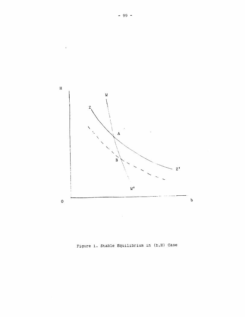
- 99 -

H

w

z

A

B

z'

W

0 b

Figure 1. Stable Equilibrium in (b,H) Case

- 100 -

CHAPTER IV

Scale Economies, Externalities, and Regional Resource Allocation

I. Introduction

This chapter presents a theoretical model of scale economies,

externalities, and efficiency of regional resource allocation. Our

purpose is two-fold. First, we want to construct a model to explain the

nature of agglomeration economies. In particular, we will focus on the

increasing productivity due to the growth of the local labor market. A

distinction will be made between internal scale economies, which will be

called simply scale economies or increasing returns to scale hereafter,

and external scale economies. The former is a phenomenon of increasing

productivity (or decreasing average cost) due to the increasing size of

the production level of an individual producer, which is under his

control . The latter refers to the productivity gain due to the size of

the economy, which presumably cannot be controlled by any single

producer. We want to analyze the nature of the external scale economies

in relation to the internal scale economies.

The second objective of the chapter is to evaluate various

urbanization policy issues in rapidly urbanizing countries. Questions

like optimal city sizes, decentralization policies and regional

investment decisions have occupied the minds of economists and policy

makers for quite a long time (see Renau'd[1981] for a comprehensive survey

on these topics). Although there has been a great deal of policy

- 101 -

discussion about them, the theory of agglomeration economies has not been

well developed. It is hoped that the model presented here will shed some

light on these issues.

Scale economies cause perfect competition to break down2 , because

the largest firm can always underbid the smaller competitors, leading

eventually to a natural monopoly. Moreover, competitive marginal pricing

yields negative profit to the producers since marginal cost will be lower

than the average cost3. One way of modeling scale economies with

competition is to assume that scale economies are completely external to

firms, so that competition can be preserved (see Helpman[1983] and

Chipman[1970] for examples of this approach). In this approach, it is

assumed that productivity is an increasing function of the aggregated

production level which is exogenous to individual firms. The typical

result of this approach is that the competitive equilibrium size is

smaller than the optimal size, because firms do not recognize the

external economies of scale created by the increase of their own activity

levels (see Shukla and Stark[1985]). This approach is unsatisfactory for

our purpose, because we are particularly interested in why such external

scale economies exist.

The second approach is the utilization of the notion of

Chamberlinian monopolistic competition to the increasing return to scale

production technology (see, for example, Krugman[1979], Weitzman[1982]).

In this approach, competition can be maintained even when firms have

increasing returns to scale technologies. As any firm's output is

substitutable to another's, the firm faces a downward sloping demand

curve. Thus, if the firm produces more in order to reduce its average

cost, it also has to reduce the price to sell the increased output. The

- 102 -

model presented in this chapter adopts the monopolistic competition

framework in labor markets to explain the external scale economy. Labor

specialization is emphasized as a source of external scale economies

rather than the sharing of infrastructure due to locational proximities.

Agglomeration economies have been recognized for quite a long

time. Fuch[1967] has found that wages in large cities are significantly

higher than wages in small cities, ceteris paribus. More recent studies,

estimating aggregated production functions of cities, consistently report

that large cities are more productive after controlling for capital labor

ratio, industrial mix, skill level of workers, and so on (see

Sveikauskas[1975], Segel[1976], Moomaw[1981], and Henderson[1983]). Also

we observe regional specializations such as concentration of financial

institutions in New York City and high-tech industry around Boston and

the "Silicon Valley". Moreover industries which require highly skilled

labor tend to concentrate more than others (Carlton[1969]). Naturally

one would turn to external scale economies for an explanation for such

phenomena.

Traditional theories for agglomeration economies are mainly based

on cost savings due to shared infrastructure and/or reduced

4transportation cost accruing to firms by locating close to one another

However, neither of the arguments is very convincing from the perspective

of a modern urban economy. First, the cost of public services and

infrastructure such as water, transportation networks, etc. is much

higher in large metropolitan areas than in small towns (Linn[1982],

Walzer[1972]). We think that agglomeration happens in spite of the

increasing marginal cost, not as a result of the decreasing marginal cost

of public service. Second, with regards to the transportation cost

- 103 -

savings argument, it should be sufficient to point out that

transportation costs are a small fraction of the total cost (less than 2

per cent) of most commodities. Thus large reductions in transportation

costs will result in only minor changes in total cost, and are not likely

to affect the locational decision of the firm.

In the following model, labor specialization is the key source of

external scale economies. 5 Labor specialization and the roundabout nature

of modern production technologies are the basic characteristics of modern

urban economies. Although geographical proximity plays an important role

in the process of urban ag-glomeration, the argument is that geographical

proximity enables producers to specialize, and thus to increase

productivity. Given the usual social practice that workers commute back

and forth between their residence and workplace on a daily basis,

specialization would be limited by the size of the urban area in which

daily commuting is possible. Although average productivity will be

increased by adopting more specialized and roundabout technologies, such

technologies can only be adopted when the market is large enough so that

they can be supported by the activities of other agents in the market.

Since an individual agent in the market can not control the size of the

market, the productivity gain through the specialization is an

externality.

There has been growing concern about the rapid urbanization and

the concentration of population in very large cities among economists and

policy makers in many developing countries. The average annual rate of

increase of urban populations in less developed countries has been over 4

per cent during the past three decades. The annual growth rate of urban

population in developed countries has been decreasing from 2.5 per cent

- 104 -

to 1.5 percent, for the same period. Since the world population has been

growing steadily by about 2 per cent annually the major thrust of

urbanization has been occurring in developing countries. Although

development planning traditionally has been carried out in sectoral

level, there has been a growing need for a national urbanization policy

in order to coordinate the planning activities in more specific spatial

context.

Nonetheless, there are conflicting views about the phenomena of

rapid urbanization. On the one hand, proponents of urbanization cite the

classical development theory by Lewis[1955] and Fei and Ranis[1964].

Those authors implicitly interpreted urbanization as a process of

releasing rural labor, which has low marginal productivity, to industrial

labor. By holding the wage at subsistence level which is lower than the

marginal productivity of the industrial sector, the economy can

accumulate capital and thus grow faster. The proponents of urbanization

sometimes use a different rationale. Planners in the industrial sector,

for example, favor the concentration of activities in order to exploit

increasing returns to scale and/or external economies. On the other

hand, congestion and pollution in high density urban areas. have been

widely recognized. The emergence of the "super-metropolis" in developing

countries has put a great deal of pressure on the utilization of new

investment in urban resources. To name a few, problems in housing,

transportation, environmental degradation, and social pathology have

become severe in those cities. It seems that new investment cannot catch

up with the growth of the population in the very large cities. The

general conclusion of negative externalities is that realized activity

will be greater than optimal activity, because agents do not take into

- 105 -

account their marginal social cost they impose on other agents (recall

the "Tragedy of the Commons"). The higher marginal costs required to

provide a given average level of urban services (such as utilities,

housing, and transportation) have been cited as a reason for

decentralization policies.

We make no pretense of generality. Specific assumptions will be

made in order to make the argument clear and simple. In Section II, we

will develop a model of labor specialization. Then, section III

incorporates negative externalities to examine the properties of optimum

city size. In Section IV, we apply the model to evaluate the efficiency

characteristics of city growth and allocation of resources in a system of

cities. Conclusions are offered in section V.

II. The basic model

1. Assumptions

Let us consider a closed economy of a continuum of

workers-cum-consumers with aggregate size N (see Figure 1). Workers are

indexed on a circle of a unit length with uniform density. Since the

circle has the unit length, the density is also N. The index represents

the worker's skill characteristic. Sometimes we will call the index

location and the difference between two indices distance. Notice that

terms like "location" and "distance" do not have any geographical

meanings.6 There is no a priori superiority or inferiority among workers'

skills. The size of the difference between the indices of any two

workers represents how different they are. Obviously the difference

ranges from zero to one half. Every worker supplies one unit of labor

- 106 -

provided that the net wage offer is greater than or equal to his

reservation wage.

We assume that all the workers in the economy have the same

reservation wage wo. The reservation wage reflects either the utility of

leisure or the domestic productivity of a worker. In the following

discussion, wo is interpreted as domestic productivity which a worker

gets when he works for himself. We call this situation self-sufficient

autonomy.

There are also firms in the economy. Since we do not allow

multi-plant firms, we can identify firms without any confusion. Firms

are assumed to produce homogeneous goods, which are sold in the

competitive output market. The output price is normalized to one.

Technologies are also indexed on the unit circle. The index of the

technology represents the most productive skill characteristic. The

firms can choose their technologies in the long run, but not in the short

run (long run and short run will be defined later). Since the

technologies only differ by their most productive skill characteristics,

we can unambiguously identify the firm with its most productive skill

characteristic. We shall call the characteristic the firm's location.

The mismatch between the location of jobs and workers (i.e. the

difference between workers' skill and firm's most desirable skill) is one

of the most essential parts of the model. If a worker works for a firm

located at a distance t, then there will be a training cost of 2 c(t) or

loss of production incurred. We shall assume that the cost will be borne

equally by the worker and the firm 7, and c(t) is linear with the distance

between the worker and the firm:

- 107 -

c(t) = kt (2.1)

Notice that we have already normalized that c(0) = 0. The parameter k

represents the degree of substitutability among workers. High k implies

that the production requires more specific type of labor. The shared

payment of the training cost ensures that both workers and firms have the

8incentive to have the better matching partners

To avoid the complication of substitution between productive

factors, we shall assume that labor is the only productive factor. The

firm has, what we call, roundabout technology, with the minimum efficient

scale (M) and the constant marginal product (b). It is clear that the

technology has an increasing returns to scale. More specifically, we

assume the production function has the form of:

Y= 0 , if X < M (2.2.a)

b (X - M), if X > M, (2.2.b)

where Y is output, and X is the labor input normalized to the equivalent

labor with the firm's most desirable skill characteristic. The

normalization is assumed to have the following functional form:

x = x(t) (1 - c(t)/b) (2.2.c)

where x(t) is the amount of labor with the distance t, and x is the

normalized labor unit, and c(t) is the value of the firm's share of the

training cost due to the difference. Total labor input (X) is just the

- 108

sum of the normalized labor (x) of the workers.

We will call the situation short run when there is a fixed number

of firms (m). As we have indicated, firms do not change their location

in the short run. Wage offer is the only short run decision variable of

the firm. If there is a positive short run profit, then entry will

occur. If short run profits are negative, firms will exit. Assuming

that there are no costs of relocating firms, competition among firms will

result in that all the firms get zero profit. The situation that the

number of firms (m), and thus, the distance between the neighboring firms

(2H) are determined endogenously by the zero profit condition will be

called long run.

We are mainly interested in the monopolistically competitive9

long run symmetric1 0 Nash'' equilibrium. By monopolistic competition, we

mean that every worker in the economy has at least two firms which can

pay the net wage higher than the reservation wage (i.e., w - c(H) > wo).

By symmetry, we mean that all the firms offer the same wage and the

distances between any two neighboring firms is the same. A firm will

choose the location and wage offer. A worker will choose the firm he

will work for by maximizing his net wage (wage offer minus his share of

the training cost), provided that it is greater than or equal to the

reservation wage w.. The firm makes its wage offer by assuming that

other firms' wage offers will be held constant. In the game theory

language, firms will play Stackelberg leader towards workers and play a

Nash strategy vis-a-vis the other firms. Workers are Stackelberg

followers to the firms.

2. Monopolistically competitive long run symmetric Nash equilibrium

- 109 -

There is a unique equilibrium in this model. To solve for the

equilibrium, let us first consider a firm's profit maximization problem

in the short run. Suppose there are m firms, and all the neighboring

firms are equally spaced with distance 2H. Thus, we have:

2mH = 1 (2.3)

Since all the firms are symmetric, we can choose a representative firm.

Its location can be normalized to zero without any loss of generality.

Suppose that other firms wage offers are all fixed at W. The

representative firm will want to choose its wage offer w. Consider a

worker located between the representative firm and any of its two

neighboring firms. Since the situations are identical in both

directions, we can consider only one side. Let us denote the distance

between the worker and the representative firm with wage offer w as d.

Then for the marginal worker who is indifferent between working for the

representative firm and the other adjacent firm, the net wages for the

two firms must be equal. That is to say:

w - c(d) = w - c(2H -d) (2.4)

where d is the location of the marginal worker. Given that the other

firms' wage offers are all equal to w, the firm will choose the wage

offer to maximize its profit, that is:

max b [ 2Nd - M ] - 2N [ wd + fec(t) dt ] (2.5)

- 110 -

Since the number of workers of the representative firm is a

function of its wage offer, eq.(2.4) can be regarded as a constraint to

the firm's maximization problem, eq.(2.5). We can solve eq.(2.4) for d,

and substitute it in eq.(2.5). Then we get the first order condition of

profit maximization by differentiating with respect to w and setting it

equal to zero. Evaluating the first order condition at w = w (and d = H)

implied by the symmetry assumptions of the equilibrium, we get:

b - kH = w + 2kH (2.6)

with c(t) given by eq.(2.1). Eq.(2.6) states that the marginal value

product is equal to the marginal outlay at the margin. The left hand

side is the marginal product of the marginal worker who produces b while

incurring a training cost of kH. Since the output price is one, it is

the marginal value product. If the firm hires the marginal worker, then

it pays the premium of 2kH over the prevailing wage, because it has to

attract the worker away from the neighboring firm. The equilibrium wage

offer is lower than the marginal productivity, because the firm has a

local monopsony power, i.e., if it increases its wage offer then it can

attract more workers from the neighboring firms.

Substituting eq.(2.6) into eq.(2.5), we get the profit for a firm

(p) given the number of firms in the market:

p = 5kN / 4m 2 - bM (2.7)

It is immediately clear that if there are fewer firms in the market then

the profit per firm will be higher. In the long run, however, the profit

- 111 -

will be driven to zero, with free entry, exit, and no adjustment cost of

relocating firms.

Imposing the zero profit condition, we get:

m = 1/2 5kN/bM (2.8.a)

H = ~bM/kNN (2.8.b)

w = b - 31 bkM/5N (2.8.c)

By examining eq.(2.8.a), the equilibrium number of firms (m) will be

higher if the training cost (k) is high, if the minimum efficient scale

(M) is low, if marginal productivity is low, and if the size of the

market (N) is large. We call the economy more specialized if there are

more firms around. Notice that the specialization in this model is the

specialization of labor and production technologies rather than the

variety of outputs. It would be useful to examine the extreme cases of

eq.(2.8). If M = 0, i.e., production is divisible into infinitesimal

units, then m =o , and w = b suggesting that the economy degenerates to a

small scale self-sufficiency type. On the other hand, if k = 0, i.e.,

workers are homogeneous, then economy becomes a natural monopoly

situation.

It is worthwhile to note that net wages are not equal among

workers. Workers who are located closer to their firms enjoy higher net

wages, since they pay less for training. This follows from the

assumption that workers cannot change their locations, and thus, there is

no choice of specialization by workers. The most appropriate index for

welfare is the average net wage payment, which will be denoted by W:

- 112 -

W = b - 7/2 bkM/5N (2.9)

Notice that W can be interpreted as the average productivity per worker

of the economy, since firms get zero profit. 12 By differentiating

eq.(2.9), we get the basic comparative static results:

dW/db > 0 (2.10.a)

dW/dk < 0 (2.10.b)

dW/dM < 0 (2.10.c)

dW/dN > 0 (2.10.d)

Thus, the average productivity will be higher when the marginal

productivity is high, training cost is low, minimum efficient scale is

small and the size of the market is large. Our main interest rests on

eq. (2.10.d) which shows that the average productivity increases with the

size of the market. It is clear that the average productivity is bounded

from above by the marginal productivity, which it approaches

asymptotically as the size of the market goes to infinity.

From eq.(2.9), we can see that there exists a minimum market size

in which monopolistically competitive labor market economy is viable (the

market wage is greater than the reservation wage so that specialization

can take place). Let us denote the minimum size of the market No. The

condition that the net wage of all workers is greater than the

reservation wage (w - kH > wo) implies that N > No, where,

No = 5bkM / 16(b-wo) 2 (2.11)

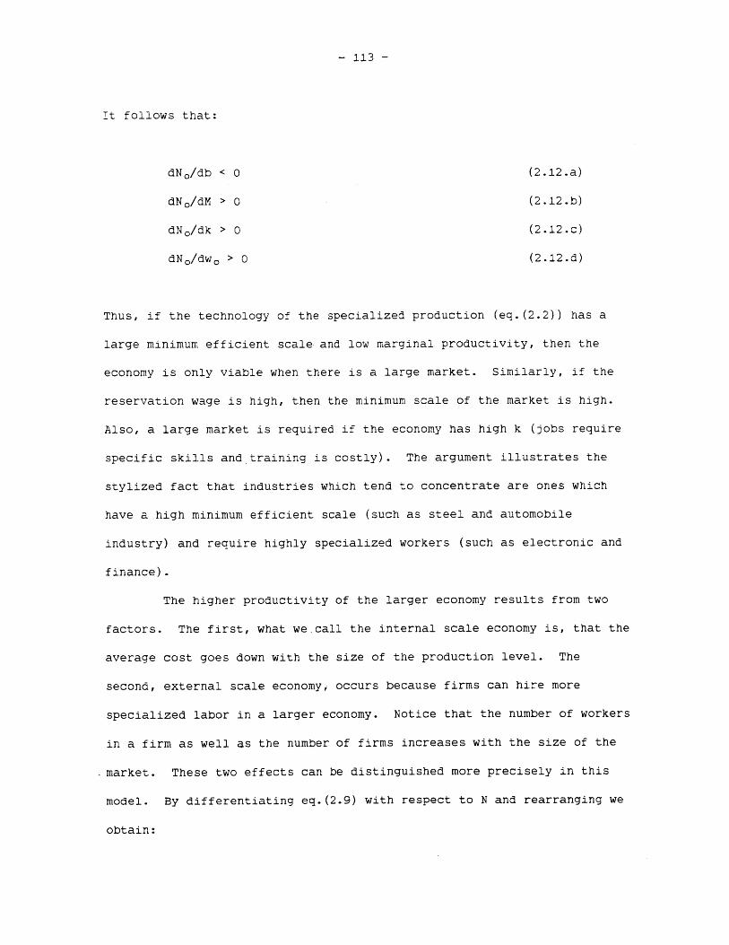
- 113 -

It follows that:

dNo/db < 0 (2.12.a)

dNo/dM > 0 (2.12.b)

dN./dk > 0 (2.12.c)

dNO/dwO > 0 (2.12.d)

Thus, if the technology of the specialized production (eq.(2.2)) has a

large minimum efficient scale and low marginal productivity, then the

economy is only viable when there is a large market. Similarly, if the

reservation wage is high, then the minimum scale of the market is high.

Also, a large market is required if the economy has high k (jobs require

specific skills and training is costly). The argument illustrates the

stylized fact that industries which tend to concentrate are ones which

have a high minimum efficient scale (such as steel and automobile

industry) and require highly specialized workers (such as electronic and

finance).

The higher productivity of the larger economy results from two

factors. The first, what we.call the internal scale economy is, that the

average cost goes down with the size of the production level. The

second, external scale economy, occurs because firms can hire more

specialized labor in a larger economy. Notice that the number of workers

in a firm as well as the number of firms increases with the size of the

market. These two effects can be distinguished more precisely in this

model. By differentiating eq.(2.9) with respect to N and rearranging we

obtain:

- 114 -

dW/dN = (bM/N 2 ) (7m/10) (2.13)

The first term of the right hand side of eq.(2.13) refers to the

productivity gain by increasing returns to scale. To see this, one may

divide eq.(2.1.b) by X in order to get the average product of a worker;

differentiate with respect to X; and evaluate at X = N. The second term

refers to the productivity gain by external scale economy. Although the

productivity gain by external scale economy increase with the number of

firms (and thus, with the size of the market), the more rapid decline of

the productivity gain due to the internal scale economy will drive the

total effect to zero as the market size goes to infinity. The basic

reason of the external scale economy in this model is that firms will be

able to recruit more specialized workers to reduce the training cost. In

other words, there will be better matches between jobs and workers in

larger markets.

From the worker's point of view, the gain of the net wage has two

components. The first is that the worker gets the higher wage offer in

the larger market, because productivity is higher. The second is that

the average cost of a job mismatch is reduced in the large market. On

average, workers get better jobs which require lower training costs.

Given the functional specification of the model the former is six times

greater than the latter.

III. Congestion externality and optimal city size

The purpose of this section is to introduce negative

externalities into the model developed in the previous section in order

- 115 -

to show the existence of the optimal city size. The basic result of the

model of the previous section is that average productivity increases with

the size of the market given increasing returns to scale technologies,

heterogeneous labor and technologies. It implies that the city will grow

indefinitely. However, such extreme agglomeration is rarely observed in

reality. We observe that cities stop growing beyond certain points. A

discussion of possible explanations of stabilization follows. We will

discuss the points not pursued in this chapter first.

First of all, the internal scale economies may vanish. With the

expansion of the organization, the cost of control and management may

increase so that the production function becomes concave. Although the

model does not relate increased labor specialization to lower production

efficiency in our model, internal scale diseconomies may eventually lower

the average productivity of workers. In the model of the previous

section, the technology will approach constant returns to scale as the

firm size becomes large. Although the external scale economy increases

with the size of the market (thus unbounded), the average productivity is

bounded by the marginal productivity. Put differently, the average

productivity is bounded by the technology even with the unbounded

external scale economy.

A more compelling reason for the stabilization , however, comes -

from the physical consequence of the concentration of economic

activities. The price of fixed resources, particularly land, will rise

with the increased size of the market. It is well documented that urban

rent increases with the size and density of the urban area. The increase

of rent will cause three effects on the welfare of the residents. The

first effect is that with higher price of land, consumers will substitute

- 116 -

away from land to other goods to equate the marginal rate of substitution

to the price ratio. With a given income, this causes decline in the

welfare of the residents. Second, since land is also a productive

factor, cost of production will rise ceteris paribus. Thus prices of

consumer goods will go up, further lowering the utility of the residents.

The third effect is that the higher rents will be distributed to land

owners in the economy, and thus, increase the welfare of the owners.

This inflationary consequence of urbanization through the pecuniary

externality of rising rent will be deliberately avoided in the following

discussion in order to maintain a single productive factor model.

More specifically, the two stabilizing forces described above are

natural market outcomes. Since these effects do not change the

efficiency characteristics of the economy, we will concentrate on genuine

externalities prevalent in the urban economy such as congestion and

pollution. As the density of economic activity goes up, the level of

interference among the agents over the limited urban resources will grow

up. A typical example is traffic congestion. With the inability of the

market to internalize those externalities, negative externalities may be

associated with the size of the.market. We shall incorporate the

negative externality in the model.

In particular, we will assume that- the negative externality works

through the firms' production function by lowering the marginal

productivity of workers (b) as the market size increases (N). In other

words, b is to assumed to be a function of N rather than a constant. We

will call b(N) a congestion function. The agents regard b to be constant

since individual agents cannot significantly influence the size of the

market. Specifically, we will assume that the congestion function

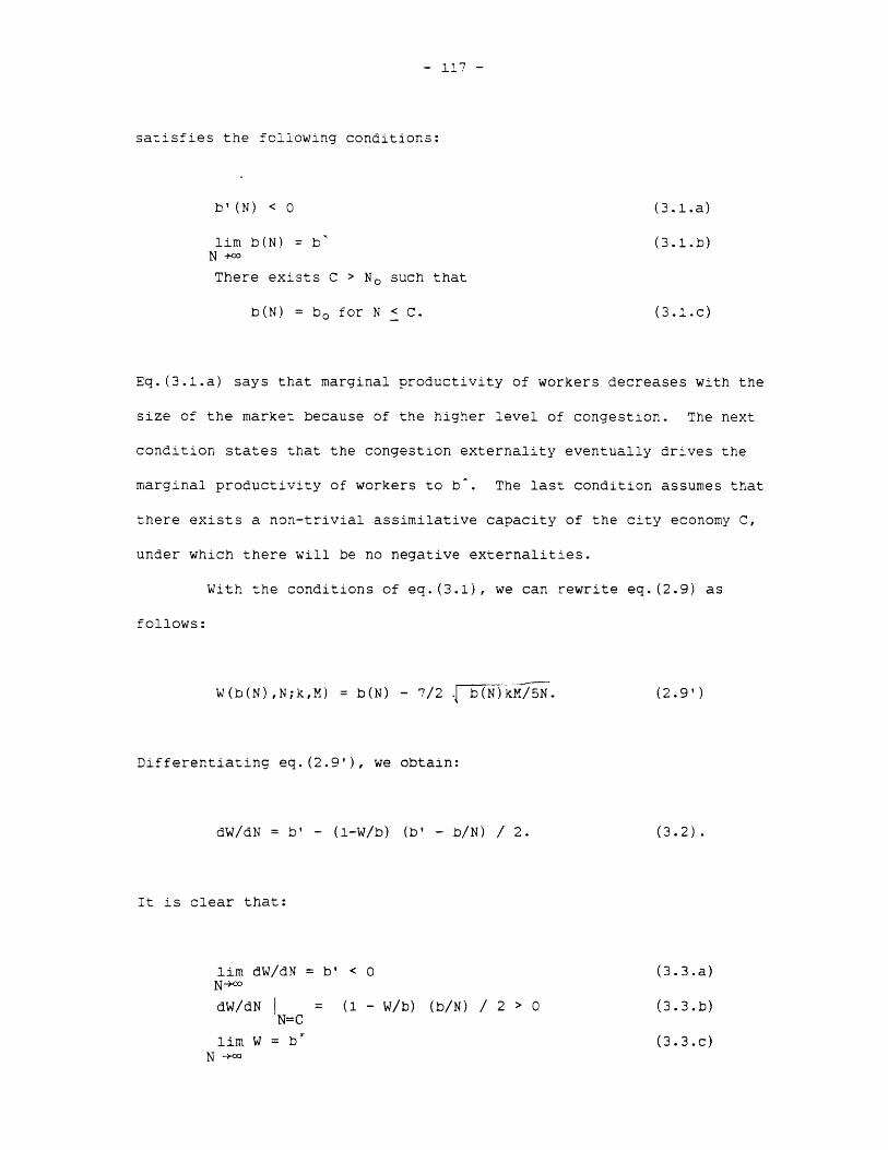
- 117 -

satisfies the following conditions:

b'(N) < 0 (3.1.a)

lim b(N) = b' (3.1.b)N +oo

There exists C > No such that

b(N) = be for N < C. (3.1.c)

Eq.(3.1.a) says that marginal productivity of workers decreases with the

size of the market because of the higher level of congestion. The next

condition states that the congestion externality eventually drives the

marginal productivity of workers to b. The last condition assumes that

there exists a non-trivial assimilative capacity of the city economy C,

under which there will be no negative externalities.

With the conditions of eq.(3.1), we can rewrite eq.(2.9) as

follows:

W(b(N),N;k,M) = b(N) - 7/2 F b(NIkY./5N. (2.9')

Differentiating eq.(2.9'), we obtain:

dW/dN = b' - (1-W/b) (b' - b/N) / 2. (3.2).

It is clear that:

lim dW/dN b' < 0 (3.3.a)

dW/dN = (1 - W/b) (b/N) / 2 > 0 (3.3.b)N=C

lim W = b. (3.3.c)N -o

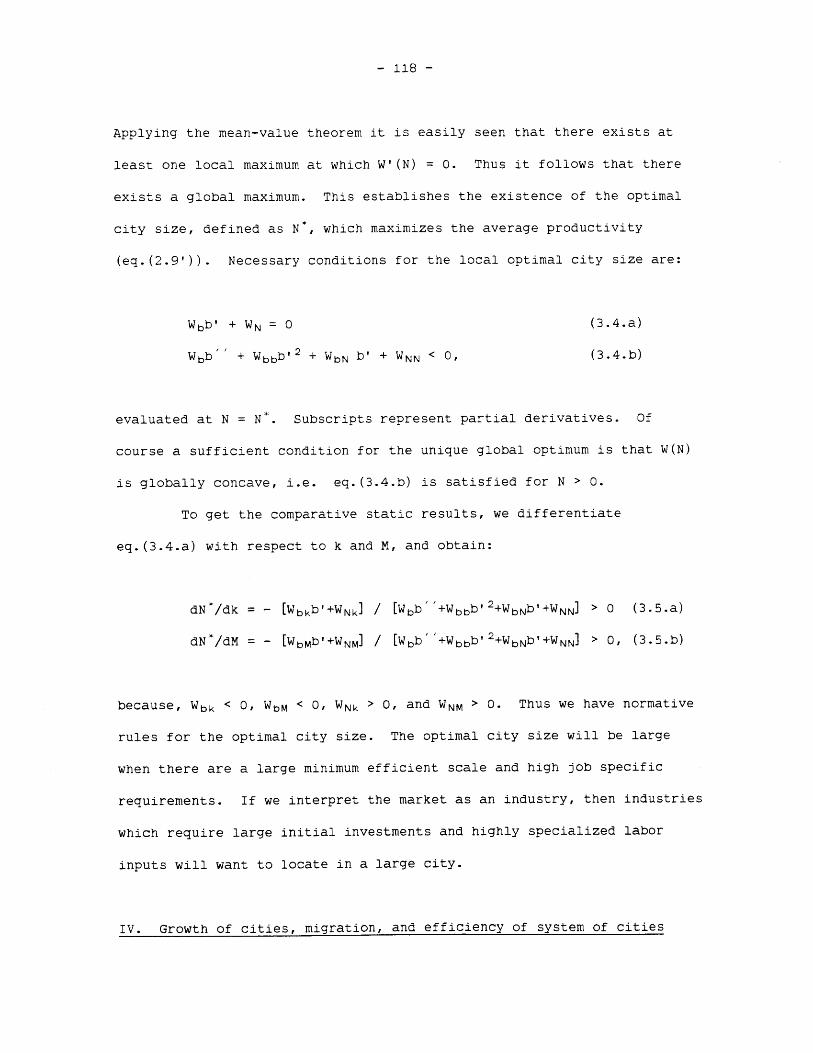
- 118 -

Applying the mean-value theorem it is easily seen that there exists at

least one local maximum at which W'(N) = 0. Thus it follows that there

exists a global maximum. This establishes the existence of the optimal

city size, defined as N*, which maximizes the average productivity

(eq.(2.9')). Necessary conditions for the local optimal city size are:

Wbb' + WN = 0 (3.4.a)

Wbb'' + Wbbb' 2 + WbN b' + WNN < 0, (3.4.b)

evaluated at N = N*. Subscripts represent partial derivatives. Of

course a sufficient condition for the unique global optimum is that W(N)

is globally concave, i.e. eq.(3.4.b) is satisfied for N > 0.

To get the comparative static results, we differentiate

eq.(3.4.a) with respect to k and M, and obtain:

dN /dk = - [Wbkb'+WNk] / [Wbb' +Wbbb'2+WbNb'+WNN > 0 (3.5.a)

dN*/dM = - [WbMb'+WNM / [Wbb' +Wbbb'2+WbNb'+WNN > 0, (3.5.b)

because, Wbk < 0, WbM < 0, WNk > 0, and WNM > 0. Thus we have normative

rules for the optimal city size. The optimal city size will be large

when there are a large minimum efficient scale and high job specific

requirements. If we interpret the market as an industry, then industries

which require large initial investments and highly specialized labor

inputs will want to locate in a large city.

IV. Growth of cities, migration, and efficiency of system of cities

- 119 -

We have examined the model in the context of a closed economy.

An important- question is the behavior of the economy in a system of

cities. In this section, we shall allow migration among regions. By

region, we mean an integrated urban labor market or homogeneous rural

area. We assume that the migration rate is linear with the net wages

differentials between the two regions:

0

N = e (W - WO), (4.1)

where the "dot" represents a time derivative. Notice that we implicitly

assume risk neutrality. Variations of eq.(4.1) have been estimated by

many authors (see Todaro[1976] and Yap[1977] for survey). Most of the

studies conclude that economic motivation is the major determinant of

migration. In order to focus the discussion on migration, we shall

assume that there is no natural growth of population. We will divide the

discussion in two subsection. First, we examine the growth of the

economy in an open region. The key assumption here is that there is an

infinite supply of migrants at a fixed utility level. This assumption

reflects the notion of "unlimited supply of labor" in the classical

development theory. Thus, this subsection is more relevant for the

rural-to-urban migration. In the second sub-section, we examine the

closed region case, in which regional wages adjust the migration process.

It is more relevant for the urban-to-urban migration.

1. Growth of cities in an open region

First, let us assume that migration is costless. Open region

assumption implies that Wo is fixed. We will call the background region

- 120 -

"rural" and our economy "urban". There will be migration into or

migration out of the region depends on whether W is greater or smaller

than Wo. Let us denote the optimal wage as W* (wage level evaluated at

N'). If W(No) < WO, then there will be emigration from the city to

reduce the size of the market to zero. In this case, city has no raison

d'etre, and is of limited interest.

Without the natural growth of population of cities, W(N) can be

regarded as the "migration demand function", because it relates the size

of the city to the wage level. Assumptions of "unlimited supply of

labor" and costless migration implies that the supply curve is

horizontal.

Depending on the shape of W(N) and the size of WO, we can

identify three major cases (Figure 2). First, the city may grow

indefinitely if W(N) > WO, for N > N. (case A in Figure 2). Notice that

this situation is not likely to occur, because the horizontal supply

curve assumption will not be warranted for very large N. Second, as in

the case C, the two curves may intersect just once. Notice that

equilibrium city size is stable and always larger than the optimal city

size (W'). Third, if the curves intersect more than once (case B), then

there exist at least one stable equilibrium city size which is greater

than local optimal. This is not a surprising result. It is a standard

conclusion that the competitive equilibrium is larger than the optimum

with negative externalities.

It is also interesting to examine the cause of the instability of

the other type of equilibrium at which the migration demand function

(W(N)) cuts the supply function from below. Suppose that the city

manifests an increasing returns to scale at a equilibrium. If, for some

- 121 -

reason, the size of the urban market increases, then the urban wage will

rise through a more extensive specialization. The higher urban wage

will, in turn, attract more worker from rural area. This cumulative

process of urban growth will continue even if congestion externalities

occur. The growth will stop when the negative externalities are strong

enough to offset the agglomeration economies such that the urban wage is

equal to the rural wage.

If migration is costly (moving cost, any additional human capital

investment for the new labor market, psychological cost, and so on), then

the model behaves somewhat differently. First of all, the supply curve

will not be horizontal. It will have a U-shape, whose minimum is at the

current N. The increasing part of the curve reflects that more workers

are willing to migrate into the urban area when the urban wage is higher.

On the contrary, the decreasing part says that more workers in the urban

area will migrate out of the urban area when they are compensated more

for their out-migration. For the sake of simplicity, we assume that

urban-to-rural migration is costless so that the migration supply curve

is upward sloping. Also we assume that W(N) is globally concave (Figure

3).

Depending on the shape of the two curves, there are three main

possibilities. In the first case, migration may not occur at all, if

W(N) is smaller than the sum of Wo and migration cost (case A in Figure

3). Case A is more likely to occur when the migration cost is high

and/or No is large (i.e., b is small, M is large, k is large, and wo is

large). Second, there may be a stable equilibrium in which the

equilibrium city size is smaller than the optimal size (case B). Case B

is more likely to happen if the migration cost is moderate and/or N* is

- 122 -

large (k is large, M is large, b is large, and w. is small). In the

third case (case C), there will be a stable equilibrium in which the

equilibrium city size is greater than the optimal city size. This case

will happen if the migration cost is low and N' is small (i.e., k is

small and M is small).

2. Growth of cities in a closed region

We now turn to the question of the growth of cities in a closed

region, in which wages can adjust to equilibrate the migration flow. To

simplify the argument, we consider the two city case only. We assume

that the total number of workers is fixed at N. Maintaining the

assumption of costless migration of workers, we can describe the two-city

system with the following set of equations:

W1 = W1 (b 1 (N 1 ),N 1 ; M1 ,k 1 ) (4.2.a)

W2 = W2 (b 2 (N 2 ),N 2 ; M2 ,k 2 ) (4.2.b)

N 1 = - N 2 = e(W 1-W 2) (4.2.c)

N1 + N 2 = N (4.2.d).

Then, one can immediately notice that there are possibilities of multiple

equilibria such that:

W1 (N 1 ) W2 (N 2 ) (4.3.a)

N1 + N 2 = N. (4.3.b).

The local stability condition for the distribution of workers is:

- 123 -

W 1 '(N1 ) + W2 '(N 2 ) < 0. (4.4)

Let us name N such that N 1 < N 2 - Suppose that two cities are symmetric,

i.e., W 1 (.) = W 2 (-), and W(.) is globally concave, then it is easy to

see that:

N1 < N* < N 2 - (4.5)

The significant result is that the bootstrapping of inefficient

allocation of workers between the two regions can be easily maintained if

the stability condition is satisfied. In effect the stability condition

states that the economies of scale of the smaller city is smaller than

the diseconomies of scale of the larger city. This is exactly the

situation that the migration from the larger city to the smaller city is

socially desirable.

This point can be illustrated by using Figure 4. Provided that

N1 + N 2 = N, the situation (W, N 1, N 2 ) is a steady state equilibrium,

because W(N 1 ) = W(N 2)- Suppose that the local stability condition

(eq.(4.4)) is satisfied at the equilibrium. Moving workers from the

larger city to the smaller city is a Pareto improvement, because the net

wages of both cities will be higher than before. But this cannot be

sustained because workers will migrate back from the small city to the

large city in order to get the higher wage. Thus, it is difficult to get

out of the inefficient steady state equilibrium. One can apply this

dynamic analysis to the case of rapidly urbanizing countries. If the

economy follows the pattern of unlimited supply of workers in the earlier

stage of the urbanization process, our analysis of the closed region will

- 124 -

apply. In other words, there are always danger that large cities will be

too large. Even when the wages of smaller regions increase to catch up

with the larger city, the efficient decentralization can be easily

blocked so that large city will stay larger than optimal while smaller

cities will remain smaller than optimal.

V. Conclusion

With increasing returns to scale technology and heterogeneity of

workers and jobs, we have constructed a model of an economy which

displays external scale economies. Although the external scale economy

intensifies with the size of the market, the productivity of the economy

is bounded by the technology since the internal scale economy becomes

insignificant with the rise of production level.

Given that there exists an assimilative capacity beyond which

congestion externalities eventually drive down the marginal productivity

of workers to the lower bound b*, there exist an optimal city size which

maximizes the average productivity of the workers. If there is an

unlimited supply of workers at a given wage level outside of the economy,

the stable equilibrium is always greater than the local optimal. If the

wage function is globally concave with respect to the size of the market

(i.e., the optimal city size is unique), then the stable equilibrium is

unique, and it is always larger than the optimal city size.

Even when migration occurs to equilibrate the wages of the

regions, systems of cities can be easily bootstrapped in an inefficient

allocation of workers provided that the stability condition is satisfied.

This may exist despite wage adjustments in the cities. Policy

- 125 -

interventions to control overconcentration of large cities and planned

centralization such as growth pole type strategy are sometimes called

for.

- 126 -

Firm i Firm j_offering w offering w

d /-

Firm 2 Firm m

Firm 1

Figure 1. The basic model

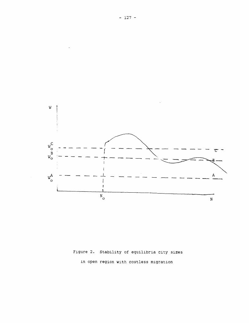
- 127 -

W

CWB

0

NN

Figure 2. Stability of equilibria city sizes

in open region with costless migration

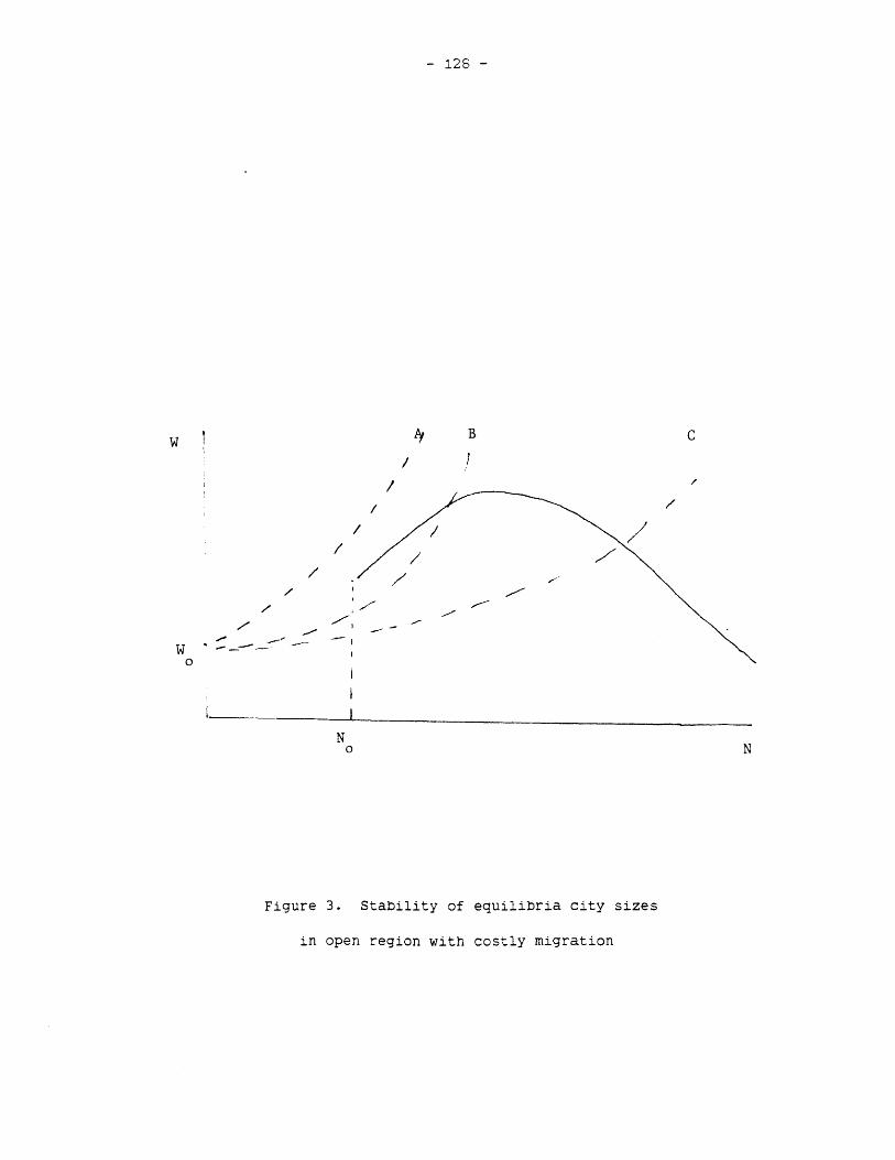
- 128 -

4 B

7-1-

W

N

Figure 3. Stability of equilibria city sizes

in open region with costly migration

WI C

N

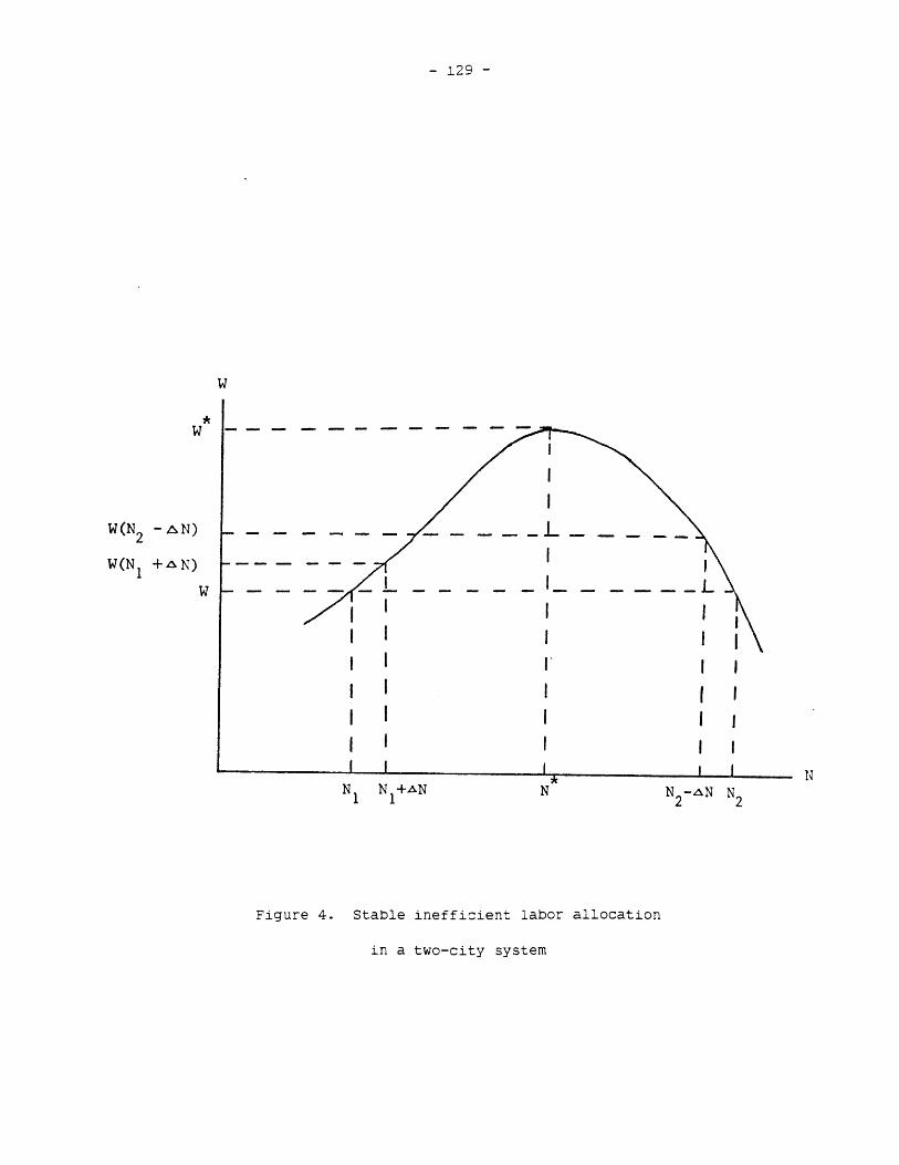
- 129 -

w

*W

W(N2 -AN)

W(NI +AN)

W I ____

I I

SI I

SI' I

I ISI ISI IS

N1N +AN N

NN 2-AN N2

Figure 4. Stable inefficient labor allocation

in a two-city system

- 130 -

Footnotes

1. There have been some micro justifications for the increasing returns

to scale besides the traditional fixed cost argument. First,

learning model of Arrow[1962] demonstrated that the

productivity increases as the production level increases.

Second, random delivery of services of factors (commonly known

as the repairman problem) can be a source of increasing returns

to scale (Arrow et. al.[1972], Rothschild and Werden[1979]) by

reducing the average probability of the idling of productive

factors.

2. The convexity assumption of production sets in the general

equilibrium model of Arrow-Debreu-Hahn precludes the

possibility of increasing returns to scale. Many of the

fundamental results (such as the existence of the competitive

equilibrium) cannot be obtained without the assumption.

3. This is a classic problem of financing and pricing of public goods

such as roads and bridges.

4. Koopmans and Beckmann[1957] have demonstrated that the optimal

assignment problem with transportation cost cannot be sustained

by the decentralized system with rents on the locations. The

basic cause of the market breakdown is the locational

externality caused by others through the transportation cost

change.

5. Jacobs[1969] provides a historical analysis of the productivity

increase through the labor specialization in urban economies.

6. It is possible to interpret the model with spatial implication.

Workers have to commute to their workplace and transportation

costs are borne equally by workers and firms. However, the

geometry of the city (circle) is not very realistic.

7. We can view this assumption in two ways. First, firms recognize a

possible worker's skill individually and bargain for the wage.

The bargaining outcome assumed here is that both parties share

the cost of training equally. The other way of viewing this is

that the worker has to pay to achieve the signal acceptable to

the firm. The firms cannot distinguish the workers ex ante,

but has to pay for the on-job-training cost, which cannot be

attributable to any workers.

- 131 -

8. If all the cost of mismatch were borne by firms, workers would have

no incentive to choose the right firms, and vice versa.

9. Depending on the parameter values, there will be the case of

monopsony equilibrium where some of the workers would not

participate in the labor market. If the size of the market is

big enough, however, we will only have the monopolistically

competitive equilibrium, which resembles the modern economy

most. The other cases are analyzed in chapter II.

10. Of course there will be possibilities of asymmetric equilibria.

Given the a priori symmetry of the assumptions of the model, we

have no interest in them.

11. There has been a criticism for the use of Nash equilibrium concept

in this type of circle model (Hart[1983]). The argument is

that the Nash assumption is not very convincing, since each

agent interacts only with two neighboring firms directly. It

is possible to get around this criticism by modifying the model

into two dimensions such that there are many neighboring firms

for each firm. See Footnote 3 in chapter II for detail.

12. It is true that the local monopsony power of firms will be reduced

in a larger market. However, since the zero profit condition

is satisfied with competition, we can safely interpret the wage

increase as the productivity increase.

- 132 -

CHAPTER V

Conclusions

The city is a complicated place. Various activities are

performed by a variety of groups of people in the city. So called "the

function of a city" is a characterization of such human activities.

Depending on the interest of a investigator, the function of a city has

been defined as a market, a political arena, an innovation center, a

place where major decisions are made, or a built environment. Given the

complex political, socio-economic and physical structure of modern

cities, it would be inevitable that any disciplinary approaches do not

capture the full spectrum of important and interesting academic and

practical issues. Since the argument provided in this dissertation takes

a very narrow viewpoint, it would be useful to examine the argument from

a broader perspective. This concluding chapter is an attempt to

synthesize the argument of the thesis with other important related

topics.

In this dissertation, we have regarded a city as a local labor

market, where workers and firms look for each other. Workers choose

firms in order to maximize net wages, whereas firms hire workers to

maximize profits. The intrinsic heterogeneity and diversity of workers

and firms are the main ingredient of the argument. The value of one

worker to a firm (or vice versa) is different from that of another, since

all workers and firms are different. One would argue that an agent is

willing to pay more for the better matching partner. The city is a place

- 133 -

in which such differences are evaluated and mediated.

The growth of a city is also a complicated phenomenon. First of

all, it is not at all clear what the term "growth" means. Vaguely

speaking, it is a process of enlarging the "size" of a city. The size of

a city may take a variety of measures such as population, employment,

output, income, capital stock, or geographical area. Nonetheless, those

measures are highly correlated with one another in a given country. We

have used the number of workers to measure the size of the market. Since

we are mainly interested in the local labor market aspect of the city,

the choice is well-suited.

The major concern of the dissertation has been the relationship

between the size of the market and the productivity of urban economy.

The term agglomeration economies loosely refers the stylized fact that

average productivity rises with the size of the market. We argued that

traditional explanations for agglomeration economies are neither rigorous

nor convincing, and suggested an alternative theory for urban

agglomeration.

We concentrated on labor specialization in order to explain

agglomeration economies. The basic argument is as follows. Given

increasing returns to scale production technologies, firms can afford to

adopt more specialized technologies in a larger and more diverse labor

market, since they will be able to find enough workers in order to

maintain their plant at an efficient level. Thus, given the distribution

of human capital characteristics, the average matching quality between

workers and jobs in larger market would be higher than in smaller market.

On the hand, workers can afford to specialize more, as there are more

diverse and specialized firms in the market. The probability of finding

- 134 -

a better matching job will be higher when there are more firms in the

market. Since they put their human capital in more specialized skills,

their productivity will increase with given level of human capital

investment cost. In short, agglomeration economies occur by two factors.

First, given that the characteristics of human capital are heterogeneous,

the average matching quality between the jobs and workers increases with

the size of the market. Second, as the size of the market increases,

workers invest their human capital in a more specialized manner so that

their productivity increases with given level of human capital cost.

In order to avoid the complication of heterogeneity of outputs,

we have assumed that firms produce homogeneous output. With homogeneous

output, we did not have to describe the demand pattern of consumers so

that we could concentrate on the labor market. However, casual

observations suggest that the diversity of products is closely related to

the diversity of workers. Therefore, it would be interesting to extend

the model to allow firms produce different products (or different

varieties) in order to examine the interaction between the labor market

and goods market.

One may hardly separate between the productivity increase due to

agglomeration economies and technological innovations. It is a well

known fact that cities, particularly large cities, are responsible for

most of the important technological innovations. One would guess that

the success of innovations are somehow associated with labor

specialization and the capacity to provide specialized goods and services

available in large cities. The aspect of this endogenous process of

innovation and agglomeration has not been addressed in this dissertation

at all.

- 135 -

For one thing, the process of innovation is not understood very

well. Questions like: How does a new innovation occur? How does it

develop? What are the determinants of successful innovations? How is it

transferred to others? are not answered adequately. Although, there is

substantial literature about information diffusion process in geography,

most of the authors are concerned about when and how the new information

arrives rather than how the new innovations occur and are adopted. More

work regarding the relationships between labor specialization,

agglomeration and innovations is suggested.

The increase of productivity and of wage has been regarded as the

driving force of the urban growth process. As the size of the city

grows, firms can exploit the increasing returns to scale technology.

Thus, average cost will decline. Such productivity increase will be

further reinforced by agglomeration economies and labor specialization.

Large cities will have higher productivity. Higher productivity will be

transmitted to higher wages. Higher wage in larger city will attract

more workers from smaller cities and rural areas. In short, the growth

of the city is unstable. Even if two cities in the same regions are

slightly different in early settlement period, the small difference in

the beginning generates big difference in later stage.

The city is an artifact through which an individual communicates

with other people effectively and efficiently. It seems clear that there

are increasing returns to scale in information processing and

dissemination. Major communication channels, public or private, go

through large cities. Newspapers, TV stations, telephone switching,

satellite stations, and other communication facilities are primarily

located in cities. The same argument applies to transportation. Major

- 136 -

interregional transportation facilities such as airports, railroad

stations, seaports, distribution centers are in large cities. This

reflects the view of central place theory. Namely, a city is a service

center for its hinterland, and every activity has a non-trivial minimum

efficient scale below which the activity cannot be sustained efficiently.

It has been a powerful conceptual framework to explain systems of

cities and city hierarchies. The central place theory gives a

theoretical underpinning for the growth pole policy. The basic idea is

that the benefits of the center will be proliferated to the hinterland.

Thus, in order to promote the economic prosperity in a region, you have

to promote the economic prosperity of the core region. The target core

region (usually medium-sized cities) are called growth poles. Most of

the practical efforts of such policies have not been very successful.

Many authors pointed out that the trickling down effect is much smaller

than expected. Cities turned out to be quite open. Namely, the

interactions between the cities in different regions are quite strong

relative to those between the cities and their hinterland.

Moreover the central place theory does not explain regional

specialization. All cities at the same hierarchy level should have

identical function, since the function of a city is determined by the

size of its hinterland. Empirically, it is far from true. We observe

that cities of similar sizes may have complete different industrial

structures and functions.

The Heckscher-Ohlin (H-0) framework, the work horse model of the

modern trade theory, provides an explanation of regional specialization.

The fundamental result of H-0 theory along with Rybczynski theorem and

Stolper-Samuelson Theorem is that the region will specialize in the

- 137 -

industry which the it has a comparative advantage. For example, if the

region is abundant in labor, it will specialize in labor intensive

industry and so on.

The H-0 theory has been criticized by some of the empirical

findings of international trade. They are: 1) Leontief paradox (the

U.S. which has the highest capital labor ratio exports labor intensive

goods and imports capital intensive goods); and 2) the bulk of the

international trade is intra-industry trade rather the inter-industry

trade. There have been attempts to include the human capital element in

order to explain the Leontief paradox. New theoretical efforts are more

concerned about increasing returns to scale, and product differentiation.

These elements are incorporated into our model. For example, one wonders

why Switzerland specializes in watches. A layman will answer that it is

because the country has a highly productive watch industry. The

productivity is high, because there are so many good watch mechanics,

precision metal cutters and other workers who are suitable for such

industry. Then the question is why there are so many of them in

Switzerland. If we accept the assumption that workers make their human

capital decision based on future earning capabilities, the workers in

Switzerland choose to be watch mechanics, because they command higher

wage. Thus, there is an element of increasing returns to scale and

instability in the argument. If a economy is specialized enough in one

industry such that its productivity is high enough, then the workers

invest their human capital in that industry so that it becomes more

productive. Rather that the neoclassical marginalist's argument that

marginal productivity will decrease with the level of production, this

argument suports the argument that marginal productivity increase with

- 138 -

the level of production.

The major function of a city changes over time. Historically,

for example, American cities before early 19the century were centers for

trade. The typical U.S. city was a place for commerce, international

trade, and trading crafts and agricultural products. After the

industrial revolution, however, it became a place for production of

various manufacturing goods. It produced textile, garment, machinery,

and other types of light and heavy manufacturing goods. Since 1960's, it

became a center for service industries. Employment in baking, insurance,

information services and other office activities now exceed the

manufacturing employment in most of the major American cities.

As the demand pattern and technologies change over time, the

local industrial structure and the labor pool must adjust. We have been

observing that many industrial cities in Northeast and Midwest of the

U.S. have economic troubles. Unemployment rates rise and household

income falls. Plant closing sometimes severely affects the local

economy. Many state and local governments have tried to promote economic

development by various fiscal incentives. The fiscal approach in general

has not been very effective, since the. firm's location decision is

affected very little by the local fiscal consideration. The

characteristic of local labor pool seems much more important determinant

of such location decisions. From the viewpoint of the model in this

dissertation, it would be worthwhile to direct incentive packages to more

specific industries which have better matching with the local labor

market. With a little adjustment cost of the existing labor pool, such

approach can generate new vitality in the local economy.

The model presented in the dissertation would serve a framework

- 139 -

to study the problems of rapid urbanization in developing countries. The

urbanization trend in developing countries have been quite impressive for

the past three decades. Besides the debate whether urbanization is

mainly by migration or natural growth, the rapid urbanization put a great

deal of pressure on the direction of regional investment policies. With

the population increase of more than 4 per cent a year, the largest

cities in developing countries lack a great deal of social

infrastructure. Housing is in great shortage. Streets are congested.

Air and water quality have fallen drastically. With heavy concentration

of people in a small number of prime cities, the national economy has to

face the trade-off between the investment in social infrastructure in

those cities and other investment in smaller cities. Since large cities

are likely to stay large, a careful national urbanization policies is

called for.

It may appear that we are trying to denounce the importance of

transportation cost and any other frictional-costs to overcome distance.

This is not the case. In fact, we have adopted a extreme assumption that

intra-urban transportation cost is zero while inter-urban transportation

cost is infinite. If we adopt a more realistic assumption, say any

transportation is neither costless nor prohibitively expensive, we might

expect a global stability in a national system of cities.

The point is, however, that there are no local stabilities in

systems of cities. The system may be (and we think it is) globally

stable, but locally unstable. For example, we do not expect New York

City will attract all the population of the U.S. (global stability).

There will be substantial number of people in Chicago, Los Angeles, and

other metropolitan areas. However, we expect one city or a few cities to

- 140 -

dominate a region (local instability). Moreover, the dominant city is a

product of insignificant differences or accidents in the beginning rather

than of the intrinsic difference among cities. It is not all clear why

Chicago rather than Gary became the regional center. Also it is not

clear why Manhattan rather than Staten Island became the Central Business

District (CBD) of New York city region. They did not have any

differences in their intrinsic endowments related to their locale.

Our philosophical underpinning is that once you get some minimum

momentum, the process continues up to a point that it cannot be sustained

globally. This viewpoint contrasts with the general equilibrium

framework of Arrow-Debreu, where the global convexity is assumed. The

fundamental welfare theorems of Arrow-Debreu model do not apply to the

case of local instability-global stability framework. There is no fine

adjustment of marginal cost (or marginal product, etc.) in a locally

unstable regime. Convexity is violated. The globally stable equilibrium

is a historical product. One cannot predict the equilibrium ex ante.

Moreover, the equilibrium will in general not be a Pareto optimal. For

example, the "qwerty" typewriter keyboard which is the most widely used

English keyboard is proven to be not efficient. However, the change to

the most efficient keyboard can be easily blocked. No individuals, or

groups, unless they are powerful enough, can induce such change. The

same kind of argument applies to the location of CBD in most of the old

cities. Is Manhattan the socially optimal location for CBD? Many people

may argue against it. It is an island, and one has to cross a bridge to

get there and so on. But, the point is that the socially inferior

equilibrium cannot be broken without significant collective action.

Moreover, it is easier to set the direction in earlier stage. Since

- 141 -

large cities are likely to stay large, this welfare implication is very

important for rapid urbanization phenomena in many developing countries.

The welfare cost of very large cities in those countries may be

significant because of misallocation of resources among regions.

- 142

Bibliography

Alonso, W.(1971), "The Economics of Urban Size," Papers and Proceedings,Regional Science Association, 26, 67-85.

Alperovich, G.(1982), "Scale Economies and Diseconomies in theDetermination of City Size Distribution," Journal of UrbanEconomics 12, 202-213.

Arnott, R.(1979), "Optimal City Size in a Spatial Economy," Journal ofUrban Economics 6, 65-89.

Arrow, K.J.(1962), "The Economic Implications of Learning-By-Doing,"Review of Economic Studies 29, 155-173.

Arrow, K.J., Levhari, D, and Sheshinski, E.(1972), "A Production Functionfor the Repairman Problem," Review of Economic Studies 39,241-49.

Baumol, W.J.(1967), "Macroeconomics of Unbalanced Growth: The Anatomy ofUrban Crises," American Economic Review 57, 414-426.

Beckmann, M.J.(1958), "City Hierarchies and the Distribution of CitySizes," Economic Development and Cultural Change 6, 243-248.

and McPherson, J.C.(1970), "City Size Distribution in aCentral Place Hierarchy: An Alternative Approach," Journal ofRegional Science 10, 25-33.

Bergsman, J. et al (1972), "The Agglomeration Process in Urban Growth,"Urban Studies 9, 263-288.

Borts, G.H.(1960), "The Equalization of Returns and Regional EconomicGrowth," American Economic Review 50, 319-347.

Borts, G.H. and Stein, P.(1964), Economic Growth in a Free Market, NewYork: Columbia University Press.

- 143 -

Carlino, G.A.(1978), Economies of Scale in Manufacturing Location:

Theory and Measurement, Laiden: Martinus-Nijhoff.

(1979), "Increasing Returns to Scale in Metropolitan

Manufacturing," Journal of Regional Science 19, 363-374.

Carlton, D.(1969), "Model of New Business Location," in Wheaton, W.C.,

(ed), Interregional Movements and Regional Growth, Urban

Institute, Washington, D.C., 1969.

Chamberlin, E.H.(1962), The Theory of Monopolistic Competition: A

Re-orientation of the Theory of Value, Cambrige: Harvard

University Press.

Chipman, J.S.(1970), "External Economies of Scale and CompetitiveEquilibrium," Quarterly Journal of Economics 84, 347-85.

Christaller, W.(1966, translated by Baskin, C.W.), Central Places in

Southern Germany, Englewood Cliffs, N.J.: Prentice-Hall.

Diamond, P.A.(1980), "An Alternative to Steady State Comparisons,"Economics Letters 5, 7-9.

(1981), "Mobility Costs, Frictional Unemployment, andEfficiency," Journal of Political Economy 89, 789-812.

(1982a), "Wage Determination and Efficiency in Search

Equilibrium," Review of Economic Studies 49, 217-227.

(1982b), "Aggregate Demand Management in Search Equilibrium,"

Journal of Political Economy 90, 881-894.

Dixit,A. and Stiglitz, J.(1977), "Monopolistic Competition and Optimum

Product Diversity," American Economic Review 67, 297-308.

Ethier, W..(1982), "Decreasing Costs in International Trade and Frank

Graham's Argument for Protection," Econometrica.

Fei, J.C.M. and Ranis, J.(1964), Development of the Labor Surplus

Economy, Homewood, IL: Richard D. Irwin, Inc.

- 144 -

Fogarty, M.S. and Garfalo, G.(1980), "Urban Size and Amenity Structureof Cities," Journal of Urban Economics 8.

Fuch, V.R.(1967a), "Differentials in Hourly Earning by Region and City

Size, 1959", National Bureau of Economic Research Occasional

Paper 101, New York.

(1967b), "Product Differences within the Service Sectors,"

NBER.

(1968), The Service Economy, New York: Columbia University

Press.

Goldfarb, R.S. and Yezer, A.M.(1976), "Evaluating Alternative Theories

of Intercity and Interregional Wage Differentials," Journal ofRegional Science 16, 345-363.

Hart, O.D.(1983), Monopolistic Competition in the Spirit of Chamberlin:

A General Model, Theoretical Economics Discussion Paper, London

School of Economics.

Helpman, E.(1984), "Increasing Returns, Imperfect Market, and Trade

Theory," R.W. Jones and P.B. Kenen (eds.), Handbook ofInternational Economics, North-Holland.

Henderson, J.V.(1974a), "The Sizes and Types of Cities," American

Economic Review 64, 640-656.

,(1974b), "Optimal City Size: The External DiseconomyQuestion," Journal of Political Economy 82, 373-388.

(1975), "Congestion and Optimum City Size," Journal of Urban

Economics 2, 48-62.

(1983), Efficiency of Resource Usage and City Size, Brown

University Working Paper No. 82-14.

Hirsh, Werner Z.(1959), "Expenditure Implications of Metropolitan Growth

and Consolidation," Review of Economics and Statistics 41,

232-241.

and Goodman, Percival, "Is There an Optimal Size of for a

- 145

City?" in M. Edel and J. Rothenberg ed., Readings in Urban

Economics, London: MacMillan.

Hirshman, A.O.(1958), The Strategy of Economic Development, New Haven:

Yale University Press.

Hoch, I.(1972), "Income and City Size," Urban Studies 9.

Hotelling, H.(1929), "Stability in Competition", Economic Journal 2,41-57.

Ijiri, Y. and Simon H. A.(1974), "Interpretation of Departures from thePareto Curve Firm-size Distribution," Journal of PoliticalEconomy 82, 315-332.

Izaraeli, 0.(1973), Differentials in Nominal Wage and Prices betweenCities, Unpublished Ph.D. Thesis, University of Chicago.

Jacobs, J.(1969), The Economy of Cities, New York: Random House.

Johnson, H.G.(1970), " A New View of the Infant Industry Argument," inI.A. McDougall and R.H. Sampe, Studies in InternationalEconomics, New York: North Holland.

Koopmans, T.C. and Beckmann, M.(1957) "Assignment Problems and the

Location of Economic Activities," Econometrica 25, 53-76.

Krugman, P.(1979), "Increasing Returns, Monopolistic Competition, andInternational Trade," Journal of International Economics 9,469-480.

Kuznets, S.S.(1965), Economic Growth and Structure, New York, Norton.

Lancaster, K.(1979), Variety, Equity, and Efficiency, New York: Columbia

University Press.

Lewis, W.A.(1954), The Theory of Economic Growth, Homewood, IL: Richard

D. Irwin, Inc.

Linn, J.F.(1982), "The Cost of Urbanization in Developing Countries,"Economic Development and Cultural Change 30, 625-648.

- 146 -

Mera, K.(1972), "On Urban Agglomeration and Economic Efficiency,"

Economic Development and Cultural Change 82, 309-325.

Mills, E.S. (1972), Studies in the Structure of the Urban Economy,

Baltimore: Johns Hopkins University Press.

and de Ferranti, D.M.(1971), "Market Choices and Optimum City

Size," American Economic Review 61, 340-345.

and K. Ohta(1976), "Urbanization and Urban Problems," in Hugh

Patrick and H. Rosovsky, eds., Asia's New Giant - How the

Japanese Economy Works, Washington, D.C.: The Brookings

Institution.

and B. Song(1979), Urbanization and Urban Problems (Studies

in the Modernization of the Republic of Korea, 1945-1975),

Harvard East Asian Monographs: 88, Cambridge, Mass.: Harvard

University Press.

Moomaw, R.L.(1976), "Productivity and City Size: A Critique of the

Evidence," Quarterly Journal of Economics 96, 675-88.

(1980), "Optimal Firm Location and City Sizes: Productivity

vs. Wages," Urban Institute Working Paper 1447-1.

Myrdal, G.(1968), Asian Drama: An Inquiry into the Poverty of Nations,

New York: Pantheon Books.

Neutze,. G. (1965), Economic Policy and the Size of Cities, Canberra:

Australian National University.

Pascal, A.H. and McCall, J.J.(1980), "Agglomeration Economies, Search

Costs, and Industrial Location," Journal of Urban Economics 8,

383-388.

Parr, J.B.(1969), "Cities Hierarchies and the Distribution of City Size:

A Reconsideration of Beckman's Contribution," Journal of

Regional Science 9, 239-253.

Renaud, B.(1981), National Urbanization Policies in Developing Countries,

Oxford: Oxford University Press.

147 -

Richardson, H. W.(1973a), The Economics of Urban Size, Heath: Boston.

(1973b), "Theory of the Distribution of City Sizes: Review and

Prospects, Regional Studies 7, 239-251.

(1977), "City Size and National Spatial Strategies in

Developing Countries," IBRD Paper 252.

Robinson, J.(1933), The Economics of Imperfect Competition, London:

Macmillan.

Rosen, K.T. and Resnik, M.(1980), "The Size Distribution of Cities: An

Examination of the Pareto Law and Primacy," Journal of Urban

Economics 8, 165-186.

Rothschild, M. and Werden, G.J.(1979), "Returns to Scale from Random

Factor Services: Existence and Scope," The Bell Journal of

Economics 10, 329-335.

Salop, S.C. (1979), "Monopolistic Competition with Outside Goods," Bell

Journal of Economic 10, 141-56.

Schaefer, G.P.(1977), "The Urban Hierarchy and Urban Area Production

Function: A Synthesis," Urban Studies 14, 315-326.

Schmandt, H.J. and Stephens, G.R.(1960), "Measuring Municipal Output,"

National Tax Journal 13, 369-375.

Scully, G.(1969), "Interstate Wage Differentials," American Economic

Review 59, 757-773.

Segel, D.(1976), "Are There Returns to Scale in City Size?", Review of

Economics and Statistics 58, 339-350.

Shefer, D.(1969), "Returns to Scale and Elasticity of Substitution by

Size of Establishment for Two-digit U.S. Manufacturing

Industries, 1958-1963," Discussion Paper No. 26, Regional

Science Research Institute.

(1973), "Localization Economies in SMSA's: A Production

Function Approach," Journal of Regional Science 13, 55-64.

- 148

Simon, H.A. (1955), "On a Class of Skew Distribution Functions,"

Biometrika 42, 425-440.

Smith, A.(1776), An Inquiry into the Nature and Causes of the Wealth of

Nations, reprinted by New York: The Modern Library, 1965.

Spence, M.(1974), Market Signalling: Information Transfer in Hiring and

Related Screening Processes, Cambridge, MA: Harvard University

Press.

(1976), "Product Selection, Fixed Costs and Monopolistic

Competition," Review of Economic Studies 43, 217-235.

Stigler, G.J.(1951), "The Division of Labor is Limited by the Extent of

the Market," Journal of Political Economy 59, 185-93.

Stuart, C. (1979), "Search and the Spatial Organization of Trading", in

Studies in the Economics of Search ed. by S. A. Lippman and

J. J. McCall, North Holland, Amsterdam.

Sveikauskas, L.(1975), "The Productivity of Cities," Quarterly Journal of

Economics 89, 393-413.

Todaro, M.P.(1976), Internal Migration in Developing Countries, I.L.O.,

Geneva.

Tolley, G.S. (1974), "The Welfare Economics of City Bigness," Journal of

Urban Economics 1, 324-45.

Vernon, R.(1960), Metropolis 1985, Cambridge, Mass.: Harvard University

Press.

Vining, D.(1976), "Autocorrelated Growth Rates and the Pareto Law : A

Further Analysis," Journal of Political Economy 84, 369-380.

(1982), "Migration between the Core and the Periphery,"

Scientific America 249, No. 12.

(1985), "The Growth of Core Region in the Third World,"

Scientific America 252, No. 4, 42-49.

- 149 -

Walzer, W.(1972), "Economies of Scale and Municipal Police Services: The

Illinois Experience," Review of Economics and Statistics 54,

431-438.

Weitzman, M.L.(1982), "Increasing Returns and the Foundations of

Unemployment Theory," Economic Journal 92, 787-804.

Wheaton, W. and Shishido, H.(1981), "Urban Concentration, Agglomeration

Economies and the Level of Economic Development," Economic

Development and Cultural Change 29, 17-28.

Will, R.E.(1965), "Scale Economies and Urban Services Requirement," Yale

Economic Essays 5, 3-60.

Williamson, J.G.(1965), "Regional Inequality and the Process of National

Development: A Description of the Patterns," Economic

Development and Cultural Change 13, No. 4, part 2.

Worcester, D.A.(1969), "Pecuniary and Technological Externality, Factor

Rents, and Social Cost," American Economic Review 59, 873-885.

Yap, L.Y.L.(1977), "The Attraction of Cities: A Review of Migration

Literature," Journal of Development Economic 4, 240-264.

Yezer, A.M.J. and Goldfarb, R.S.(1978), "An Indirect Test of Efficient

City Sizes," Journal of Urban Economics 5, 46-65.

Zipf, G.K.(1949), Human Behavior and the Principles of Least Effort,

Cambridge, Mass.: Addison-Wesley.