Tagging – more details

Reading:

D Jurafsky & J H Martin (2000) Speech and Language Processing, Ch 8

R Dale et al (2000) Handbook of Natural Language Processing, Ch 17

C D Manning & H Schütze (1999) Foundations of Statistical Natural Language Processing, Ch 10

POS tagging - overview

• What is a “tagger”?

• Tagsets

• How to build a tagger and how a tagger works– Supervised vs unsupervised learning– Rule-based vs stochastic– And some details

What is a tagger?

• Lack of distinction between …– Software which allows you to create something you

can then use to tag input text, e.g. “Brill’s tagger”– The result of running such software, e.g. a tagger for

English (based on the such-and-such corpus)

• Taggers (even rule-based ones) are almost invariably trained on a given corpus

• “Tagging” usually understood to mean “POS tagging”, but you can have other types of tags (eg semantic tags)

Tagging vs. parsing

• Once tagger is “trained”, process consists straightforward look-up, plus local context (and sometimes morphology)

• Will attempt to assign a tag to unknown words, and to disambiguate homographs

• “Tagset” (list of categories) usually larger with more distinctions

Tagset

• Parsing usually has basic word-categories, whereas tagging makes more subtle distinctions

• E.g. noun sg vs pl vs genitive, common vs proper, +is, +has, … and all combinations

• Parser uses maybe 12-20 categories, tagger may use 60-100

Simple taggers

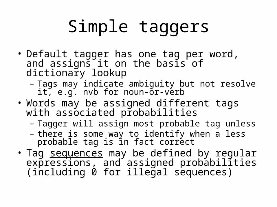
• Default tagger has one tag per word, and assigns it on the basis of dictionary lookup– Tags may indicate ambiguity but not resolve it, e.g.

nvb for noun-or-verb• Words may be assigned different tags with

associated probabilities – Tagger will assign most probable tag unless – there is some way to identify when a less probable

tag is in fact correct• Tag sequences may be defined by regular

expressions, and assigned probabilities (including 0 for illegal sequences)

What probabilities do we have to learn?

(a) Individual word probabilities:Probability that a given tag t is appropriate

for a given word w– Easy (in principle): learn from training corpus:

– Problem of “sparse data”:• Add a small amount to each calculation, so we get

no zeros

)(

),()|(

wf

wtfwtP

(b) Tag sequence probability:

Probability that a given tag sequence t1,t2,…,tn is appropriate for a given word sequence w1,w2,…,wn

– P(t1,t2,…,tn | w1,w2,…,wn ) = ??? – Too hard to calculate entire sequence:P(t1,t2 ,t3 ,t4 , …) = P(t2|t1 ) P(t3|t1,t2 ) P(t4|t1,t2 ,t3 ) …

– Subsequence is more tractable– Sequence of 2 or 3 should be enough:

Bigram model: P(t1,t2) = P(t2|t1 )

Trigram model: P(t1,t2 ,t3) = P(t2|t1 ) P(t3|t2 ) N-gram model:

ni

iin ttPttP,1

11 )|(),...,(

More complex taggers

• Bigram taggers assign tags on the basis of sequences of two words (usually assigning tag to wordn on the basis of wordn-1)

• An nth-order tagger assigns tags on the basis of sequences of n words

• As the value of n increases, so does the complexity of the statistical calculation involved in comparing probability combinations

History

1960 1970 1980 1990 2000

Brown Corpus Created (EN-US)1 Million Words

Brown Corpus Tagged

HMM Tagging (CLAWS)93%-95%

Greene and RubinRule Based - 70%

LOB Corpus Created (EN-UK)1 Million Words

DeRose/ChurchEfficient HMMSparse Data

95%+

British National Corpus

(tagged by CLAWS)

POS Tagging separated from

other NLP

Transformation Based Tagging

(Eric Brill)Rule Based – 95%+

Tree-Based Statistics (Helmut Shmid)

Rule Based – 96%+

Neural Network 96%+

Trigram Tagger(Kempe)

96%+

Combined Methods98%+

Penn Treebank Corpus

(WSJ, 4.5M)

LOB Corpus Tagged

How do they work?

• Tagger must be “trained”

• Many different techniques, but typically …

• Small “training corpus” hand-tagged

• Tagging rules learned automatically

• Rules define most likely sequence of tags

• Rules based on – Internal evidence (morphology)– External evidence (context)

Rule-based taggers

• Earliest type of tagging: two stages

• Stage 1: look up word in lexicon to give list of potential POSs

• Stage 2: Apply rules which certify or disallow tag sequences

• Rules originally handwritten; more recently Machine Learning methods can be used

• cf transformation-based learning, below

Stochastic taggers

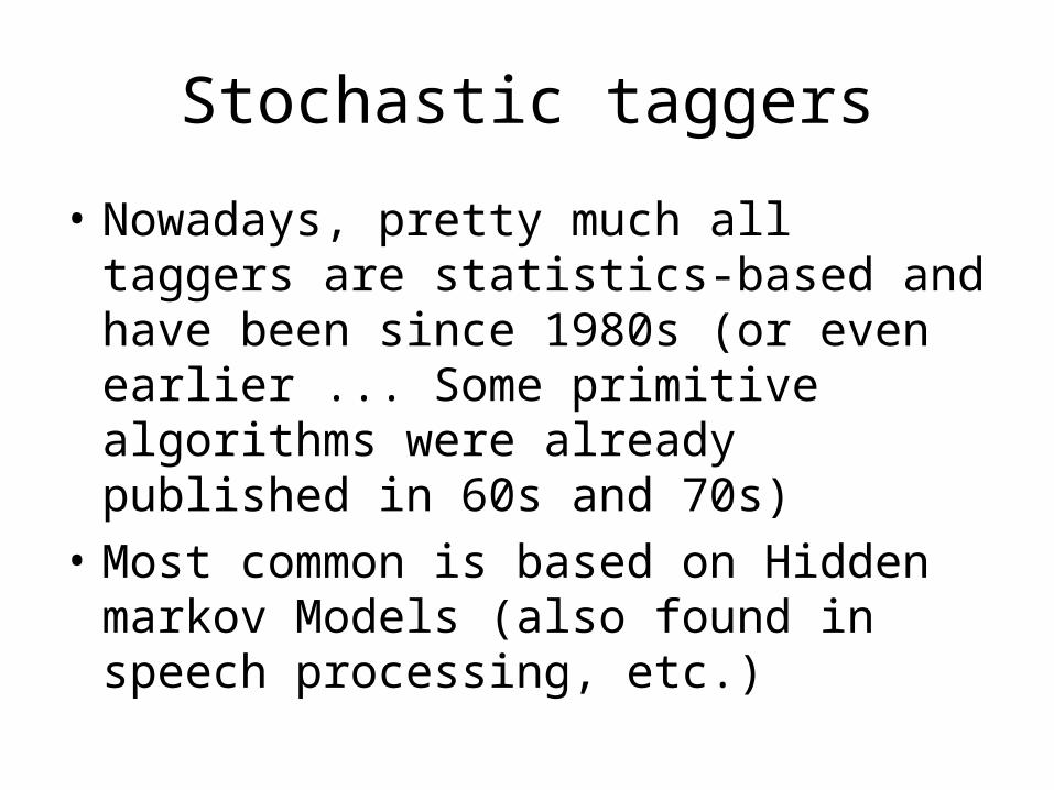
• Nowadays, pretty much all taggers are statistics-based and have been since 1980s (or even earlier ... Some primitive algorithms were already published in 60s and 70s)

• Most common is based on Hidden markov Models (also found in speech processing, etc.)

(Hidden) Markov Models

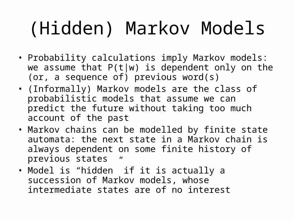
• Probability calculations imply Markov models: we assume that P(t|w) is dependent only on the (or, a sequence of) previous word(s)

• (Informally) Markov models are the class of probabilistic models that assume we can predict the future without taking too much account of the past

• Markov chains can be modelled by finite state automata: the next state in a Markov chain is always dependent on some finite history of previous states

• Model is “hidden” if it is actually a succession of Markov models, whose intermediate states are of no interest

Three stages of HMM training

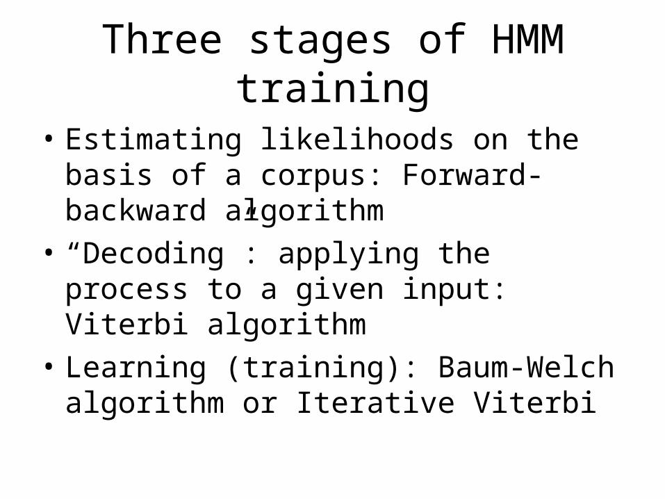
• Estimating likelihoods on the basis of a corpus: Forward-backward algorithm

• “Decoding”: applying the process to a given input: Viterbi algorithm

• Learning (training): Baum-Welch algorithm or Iterative Viterbi

Forward-backward algorithm

• Denote• Claim:

• Therefore we can calculate all At(s) in time O(L*Tn).

• Similar, by going backwards, we can get:

• Multiplying we can get:• Note that summing this for all states at a time t

gives the likelihood of w1…wL.

sstatewwPsA ttt ,1

qttt swPqsPqAsA 11

sstatewwPsB tLtt 1 sstatewwP tL ,1

Viterbi algorithm (aka Dynamic programming)

(see J&M p177ff)

ttimeatsstatewithendingsequencestateBestsQt • Denote • Claim:• Otherwise, appending s to the prefix would get a path better than Qt+1(s).• Therefore, checking all possible states q at time t, multiplying by the transition probability between q and s and the expression probability of wt+1 given s, and finding the maximum, gives Qt+1(s).• We need to store for each state the previous state in Qt(s).• Find the maximal finish state, and reconstruct the path.• O(L*Tn) instead of TL.

ttttt sQQsQ 111

Baum-Welch algorithm

• Start with initial HMM

• Calculate, using F-B, the likelihood to get our observations given that a certain hidden state was used at time i.

• Re-estimate the HMM parameters

• Continue until convergence

• Can be shown to constantly improve likelihood

Unsupervised learning

• We have an untagged corpus

• We may also have partial information such as a set of tags, a dictionary, knowledge of tag transitions, etc.

• Use Baum-Welch to estimate both the context probabilities and the lexical probabilities

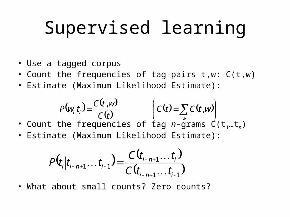
Supervised learning

• Use a tagged corpus• Count the frequencies of tag-pairs t,w: C(t,w)• Estimate (Maximum Likelihood Estimate):

• Count the frequencies of tag n-grams C(t1…tn)• Estimate (Maximum Likelihood Estimate):

• What about small counts? Zero counts?

wii wtCtC

tC

wtCtwP ,

,

11

111

ini

iniinii ttC

ttCtttP

Sparse Training Data - Smoothing

• Adding a bias:

• Compensates for estimation (Bayesean approach)• Has larger effect on low-count words• Solves zero-count word problem• Generalized Smoothing:

• Reduces to bias using:

TwC

wtCwtPwtCwtC

,

'),(,'

tovermeasureyprobabilitfwtfwwC

wtCwwtP ,,1

,11

Twtf

TwC

wCw

1,1

Decision-tree tagging

• Not all n-grams are created equal:– Some n-grams contain redundant information

that may be expressed well enough with less tags

– Some n-grams are too sparse

• Decision Tree (Schmid, 1994)

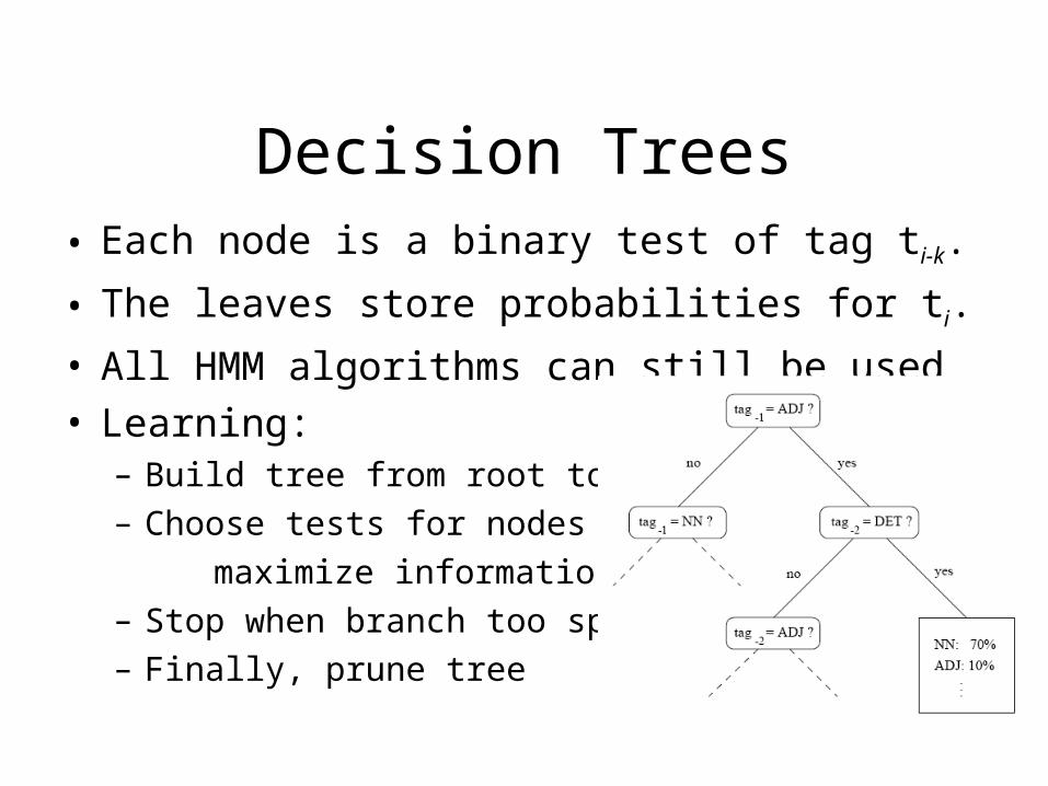
Decision Trees• Each node is a binary test of tag ti-k.

• The leaves store probabilities for ti.

• All HMM algorithms can still be used• Learning:

– Build tree from root to leaves– Choose tests for nodes that

maximize information gain– Stop when branch too sparse– Finally, prune tree

Transformation-based learning

• Eric Brill (1993)• Start from an initial tagging, and apply a

series of transformations• Transformations are learned as well, from

the training data• Captures the tagging data in much fewer

parameters than stochastic models• The transformations learned have

linguistic meaning

Transformation-based learning

• Examples: Change tag a to b when:– The preceding (following) word is tagged z– The word two before (after) is tagged z– One of the 2 preceding (following) words is

tagged z– The preceding word is tagged z and the

following word is tagged w– The preceding (following) word is W

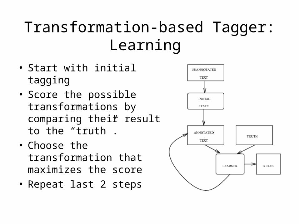
Transformation-based Tagger: Learning

• Start with initial tagging• Score the possible

transformations by comparing their result to the “truth”.

• Choose the transformation that maximizes the score

• Repeat last 2 steps