Embed Size (px)
Citation preview
Tabular Parsing
Mark-Jan Nederhof ∗
Faculty of ArtsUniversity of Groningen
P.O. Box 716NL-9700 AS Groningen, The Netherlands
Giorgio SattaDepartment of Information Engineering
University of Paduavia Gradenigo, 6/A
I-35131 Padova, Italy
1 Introduction
Parsing is the process of determining the parses of an input string accord-ing to a grammar. In this chapter we will restrict ourselves to context-freegrammars. Parsing is related to recognition, which is the process of deter-mining whether an input string is in the language described by a grammar orautomaton. Most algorithms we will discuss are recognition algorithms, butsince they can be straightforwardly extended to perform parsing, we will notmake a sharp distinction here between parsing and recognition algorithms.
For a given grammar and an input string, there may be very many parses,
∗Supported by the Royal Netherlands Academy of Arts and Sciences. Secondary affil-iation is the German Research Center for Artificial Intelligence (DFKI).
1
perhaps too many to be enumerated one by one. Significant practical dif-ficulties in computing and storing the parses can be avoided by computingindividual fragments of these parses and storing them in a table. The ad-vantage of this is that one such fragment may be shared by many differentparses. The methods of tabular parsing that we will investigate in this chap-ter are capable of computing and representing exponentially many parses inpolynomial time and space, respectively, by means of this idea of sharing offragments between several parses.
Tabular parsing, invented in the field of computer science in the periodroughly between 1965 and 1975, also became known later in the field ofcomputational linguistics as chart parsing [36]. Tabular parsing is a form ofdynamic programming . A very related approach is to apply memoization tofunctional parsing algorithms [21].
What is often overlooked in modern parsing literature is that many tech-niques of tabular parsing can be straightforwardly derived from non-tabularparsing techniques expressed by means of push-down automata. A push-down automaton is a device that reads input from left to right, while manip-ulating a stack. Stacks are a very common data structure, frequently usedwherever there is recursion, such as for the implementation of functions andprocedures in programming languages, but also for context-free parsing.
Taking push-down automata as our starting point has several advantagesfor describing tabular parsers. Push-down automata are simpler devices thanthe tabular parsers that can be derived from them. This allows us to get ac-quainted with simple, non-tabular forms of context-free parsing before wemove on to tabulation, which can, to a large extent, be explained indepen-dently from the workings of individual push-down automata. Thereby weachieve a separation of concerns. Apart from these presentational advan-tages, parsers can also be implemented more easily with this modular designthan without.
In Section 2 we discuss push-down automata and their relation to context-free grammars. Tabulation in general is introduced in Section 3. We thendiscuss a small number of specific tabular parsing algorithms that are well-known in the literature, viz. Earley’s algorithm (Section 4), the Cocke-Kasami-Younger algorithm (Section 5), and tabular LR parsing (Section 6).Section 7 discusses compact representations of sets of parse trees, which canbe computed by tabular parsing algorithms. Section 8 provides further point-
2
ers to relevant literature.
2 Push-down automata
The notion of push-down automaton plays a central role in this chapter.Contrary to what we find in some textbooks, our push-down automata do notpossess states next to stack symbols. This is without loss of generality, sincestates can be encoded into the stack symbols. Thus, a push-down automaton(PDA) A is a 5-tuple (Σ, Q, qinit , qfinal , ∆), where Σ is an alphabet, i.e., afinite set of input symbols, Q is a finite set of stack symbols, including theinitial stack symbol qinit and the final stack symbol qfinal , and ∆ is a finite setof transitions.
A transition has the form σ1v7→ σ2, where σ1, σ2 ∈ Q∗ and v ∈ Σ∗. Such a
transition can be applied if the stack symbols σ1 are found to be the top-mostfew symbols on the stack and the input symbols v are the first few symbolsof the unread part of the input. After application of such a transition, σ1 hasbeen replaced by σ2, and the next |v| input symbols are henceforth treatedas having been read.
More precisely, for a fixed PDA and a fixed input string w = a1 · · ·an ∈Σ∗, n ≥ 0, we define a configuration as a pair (σ, i) consisting of a stackσ ∈ Q∗ and an input position i, 0 ≤ i ≤ n. The input position indicateshow many of the symbols from the input have already been read. Thereby,position 0 and position n indicate the beginning and the end, respectively, ofw. We define the binary relation ` on configurations by: (σ, i) ` (σ ′, j) if andonly if there is some transition σ1
v7→ σ2 such that σ = σ3σ1 and σ′ = σ3σ2,
some σ3 ∈ Q∗, and v = ai+1ai+2 · · ·aj. Here we assume i ≤ j, and if i = jthen v = ε, where ε denotes the empty string. Note that in our notation,stacks grow from left to right, i.e., the top-most stack symbol will be foundat the right end.
We denote the reflexive and transitive closure of ` by `∗; in other words,(σ, i) `∗ (σ′, j) means that we may obtain configuration (σ′, j) from (σ, i) byapplying zero or more transitions. We say that the PDA recognizes a stringw = a1 · · ·an if (qinit , 0) `∗ (qfinal , n). This means that we start with a stackcontaining only the initial stack symbol, and the input position is initially 0,and recognition is achieved if we succeed in reading the complete input, upto the last position n, while the stack contains only the final stack symbol.
3
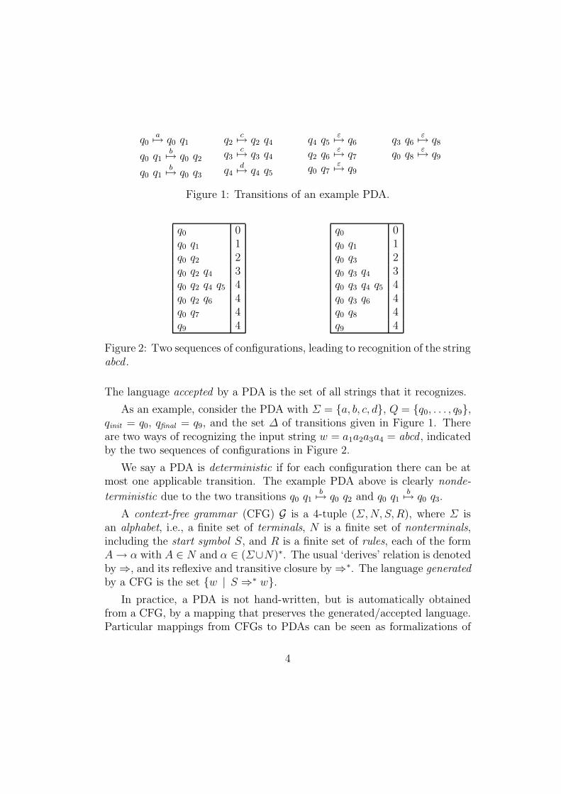
q0a7→ q0 q1
q0 q1b7→ q0 q2
q0 q1b7→ q0 q3
q2c7→ q2 q4
q3c7→ q3 q4
q4d7→ q4 q5
q4 q5ε7→ q6
q2 q6ε7→ q7
q0 q7ε7→ q9
q3 q6ε7→ q8
q0 q8ε7→ q9
Figure 1: Transitions of an example PDA.
q0 0q0 q1 1q0 q2 2q0 q2 q4 3q0 q2 q4 q5 4q0 q2 q6 4q0 q7 4q9 4
q0 0q0 q1 1q0 q3 2q0 q3 q4 3q0 q3 q4 q5 4q0 q3 q6 4q0 q8 4q9 4
Figure 2: Two sequences of configurations, leading to recognition of the stringabcd .
The language accepted by a PDA is the set of all strings that it recognizes.
As an example, consider the PDA with Σ = {a, b, c, d}, Q = {q0, . . . , q9},qinit = q0, qfinal = q9, and the set ∆ of transitions given in Figure 1. Thereare two ways of recognizing the input string w = a1a2a3a4 = abcd , indicatedby the two sequences of configurations in Figure 2.
We say a PDA is deterministic if for each configuration there can be atmost one applicable transition. The example PDA above is clearly nonde-
terministic due to the two transitions q0 q1b7→ q0 q2 and q0 q1
b7→ q0 q3.
A context-free grammar (CFG) G is a 4-tuple (Σ, N, S, R), where Σ isan alphabet, i.e., a finite set of terminals, N is a finite set of nonterminals,including the start symbol S, and R is a finite set of rules, each of the formA → α with A ∈ N and α ∈ (Σ∪N)∗. The usual ‘derives’ relation is denotedby ⇒, and its reflexive and transitive closure by ⇒∗. The language generatedby a CFG is the set {w | S ⇒∗ w}.
In practice, a PDA is not hand-written, but is automatically obtainedfrom a CFG, by a mapping that preserves the generated/accepted language.Particular mappings from CFGs to PDAs can be seen as formalizations of
4
parsing strategies.
We define the size of a PDA as∑
(σ1
v7→σ2)∈∆
|σ1vσ2|, i.e., the total number
of occurrences of stack symbols and input symbols in the set of transitions.Similarly, we define the size of a CFG as
∑
(A→α)∈R |Aα|, i.e., the total numberof occurrences of terminals and nonterminals in the set of rules.
3 Tabulation
In this section, we will restrict the allowable transitions to those of the typesq1
a7→ q1 q2, q1 q2
a7→ q1 q3, and q1 q2
ε7→ q3, where q1, q2, q3 ∈ Q and a ∈ Σ.
The reason is that this allows a very simple form of tabulation, based onwork by [17, 6]. In later sections, we will again consider less restrictive typesof transitions. Note that each of the transitions in Figure 1 is of one of thethree types above.
The two sequences of configurations in Figure 2 share a common step,
viz. the application of transition q4d7→ q4 q5 at input position 3 when the
top-of-stack is q4. In this section we will show how we can avoid doing thisstep twice. Although the savings in time and space for this toy example arenegligible, in realistic examples we can reduce the costs from exponential topolynomial, as we will see later.
A central observation is that if two configurations share the same top-of-stack and the same input position, then the sequences of steps we can performon them are identical as long as we do not access lower regions of the stackthat differ between these two configurations. This implies for example thatin order to determine which transition(s) of the form q1
a7→ q1 q2 to apply, we
only need to know the top-of-stack q1, and the current input position so thatwe can check whether a is the next unread symbol from the input.
These considerations lead us to propose a representation of sets of con-figurations as graphs. The set of vertices is partitioned into subsets, one foreach input position, and each such subset contains at most one vertex foreach stack symbol. This last condition is what will allow us to share stepsbetween different configurations.
We also need arcs in the graph to connect the stack symbols. This isnecessary when transitions of the form q1 q2
a7→ q1 q3 or q1 q2
ε7→ q3 are
applied, since these require access to deeper regions of a stack than just its
5
1 2 3 40
PSfrag replacements
S → • S + SS → S • +SS → S+ • SS → S + S •
S → • aS → a •
Sa+
qinit
qfinal
⊥ q0 q1
q2
q3
q4 q5
q6
q7
q8
q9
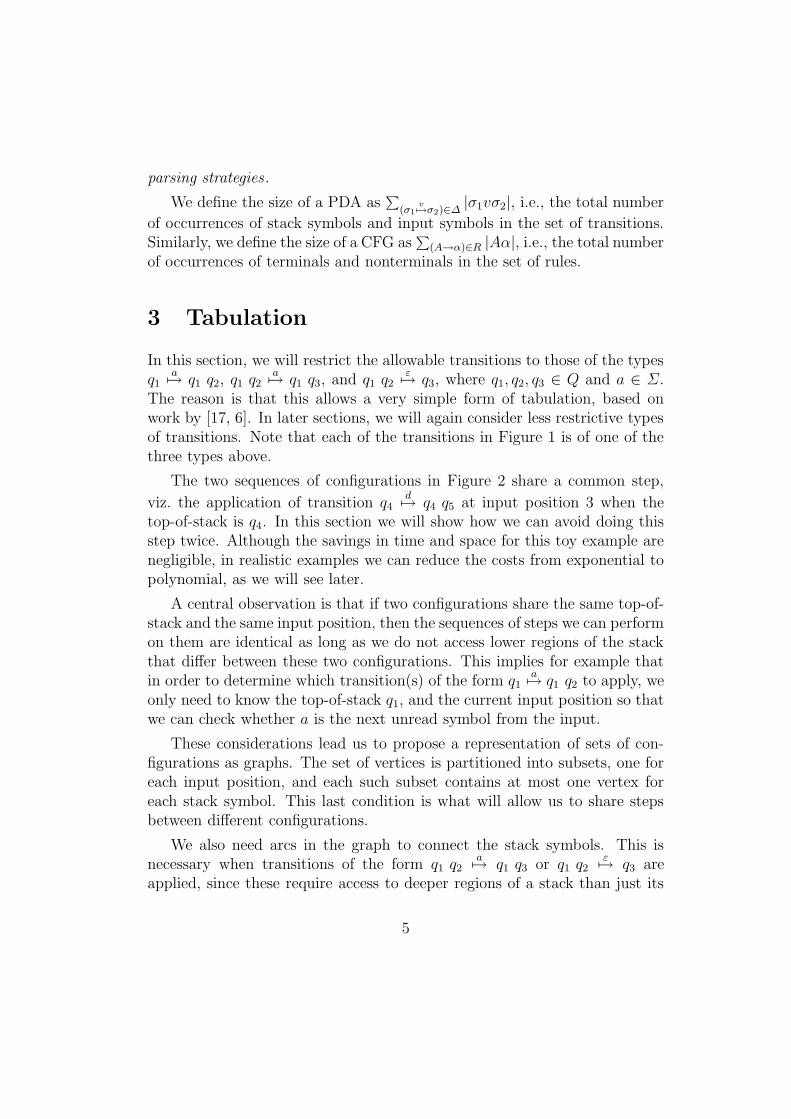
Figure 3: The collection of all derivable configurations represented as graph.For each input position there is a subset of vertices. For each such subset,there is at most one vertex for each stack symbol.
top symbol. The graph will contain an arc from a vertex representing stacksymbol q at position i to a vertex representing stack symbol q ′ at positionj ≤ i, if q′ resulted as the topmost stack symbol at input position j, and qcan be immediately on top of that q′ at position i. If we take a path from avertex in the subset of vertices for position i, and follow arcs until we cannotgo any further, encountering stack symbols q1, . . . , qm, in this order, thenthis means that (qinit , 0) `∗ (qm · · · q1, i).
For the running example, the graph after completion of the parsing pro-cess is given in Figure 3. One detail we have not yet mentioned is that weneed an imaginary stack symbol ⊥, which we assume occurs below the ac-tual bottom-of-stack. We need this symbol to represent stacks consisting ofa single symbol. Note that the path from the vertex labelled q9 in the subsetfor position 4 to the vertex labelled ⊥ means that (q0, 0) `∗ (q9, 4), whichimplies the input is recognized.
What we still need to explain is how we can construct the graph, for agiven PDA and input string. Let w = a1 · · ·an, n ≥ 0, be an input string.In the algorithm that follows, we will manipulate 4-tuples (j, q ′, i, q), where
6
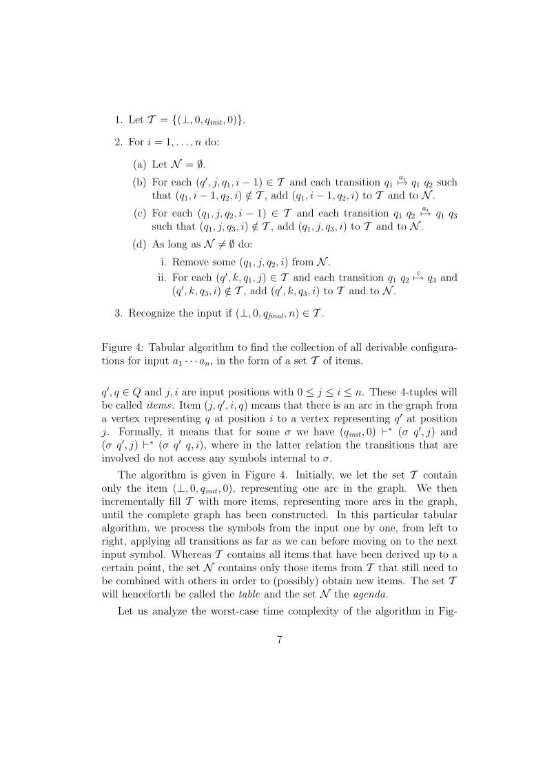
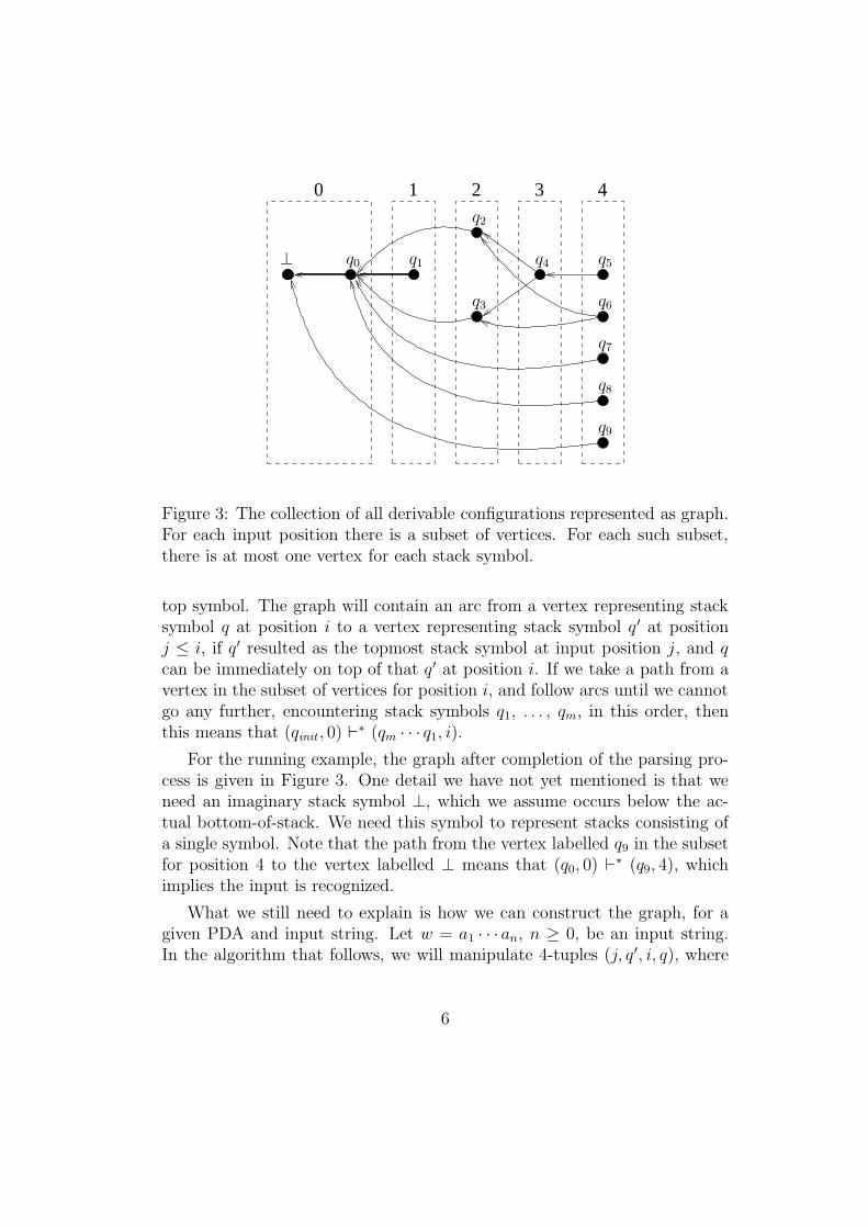
1. Let T = {(⊥, 0, qinit , 0)}.
2. For i = 1, . . . , n do:
(a) Let N = ∅.
(b) For each (q′, j, q1, i − 1) ∈ T and each transition q1ai7→ q1 q2 such
that (q1, i − 1, q2, i) /∈ T , add (q1, i − 1, q2, i) to T and to N .
(c) For each (q1, j, q2, i − 1) ∈ T and each transition q1 q2ai7→ q1 q3
such that (q1, j, q3, i) /∈ T , add (q1, j, q3, i) to T and to N .
(d) As long as N 6= ∅ do:
i. Remove some (q1, j, q2, i) from N .
ii. For each (q′, k, q1, j) ∈ T and each transition q1 q2ε7→ q3 and
(q′, k, q3, i) /∈ T , add (q′, k, q3, i) to T and to N .
3. Recognize the input if (⊥, 0, qfinal , n) ∈ T .
Figure 4: Tabular algorithm to find the collection of all derivable configura-tions for input a1 · · ·an, in the form of a set T of items.
q′, q ∈ Q and j, i are input positions with 0 ≤ j ≤ i ≤ n. These 4-tuples willbe called items. Item (j, q′, i, q) means that there is an arc in the graph froma vertex representing q at position i to a vertex representing q ′ at positionj. Formally, it means that for some σ we have (qinit , 0) `∗ (σ q′, j) and(σ q′, j) `∗ (σ q′ q, i), where in the latter relation the transitions that areinvolved do not access any symbols internal to σ.
The algorithm is given in Figure 4. Initially, we let the set T containonly the item (⊥, 0, qinit , 0), representing one arc in the graph. We thenincrementally fill T with more items, representing more arcs in the graph,until the complete graph has been constructed. In this particular tabularalgorithm, we process the symbols from the input one by one, from left toright, applying all transitions as far as we can before moving on to the nextinput symbol. Whereas T contains all items that have been derived up to acertain point, the set N contains only those items from T that still need tobe combined with others in order to (possibly) obtain new items. The set Twill henceforth be called the table and the set N the agenda.
Let us analyze the worst-case time complexity of the algorithm in Fig-
7
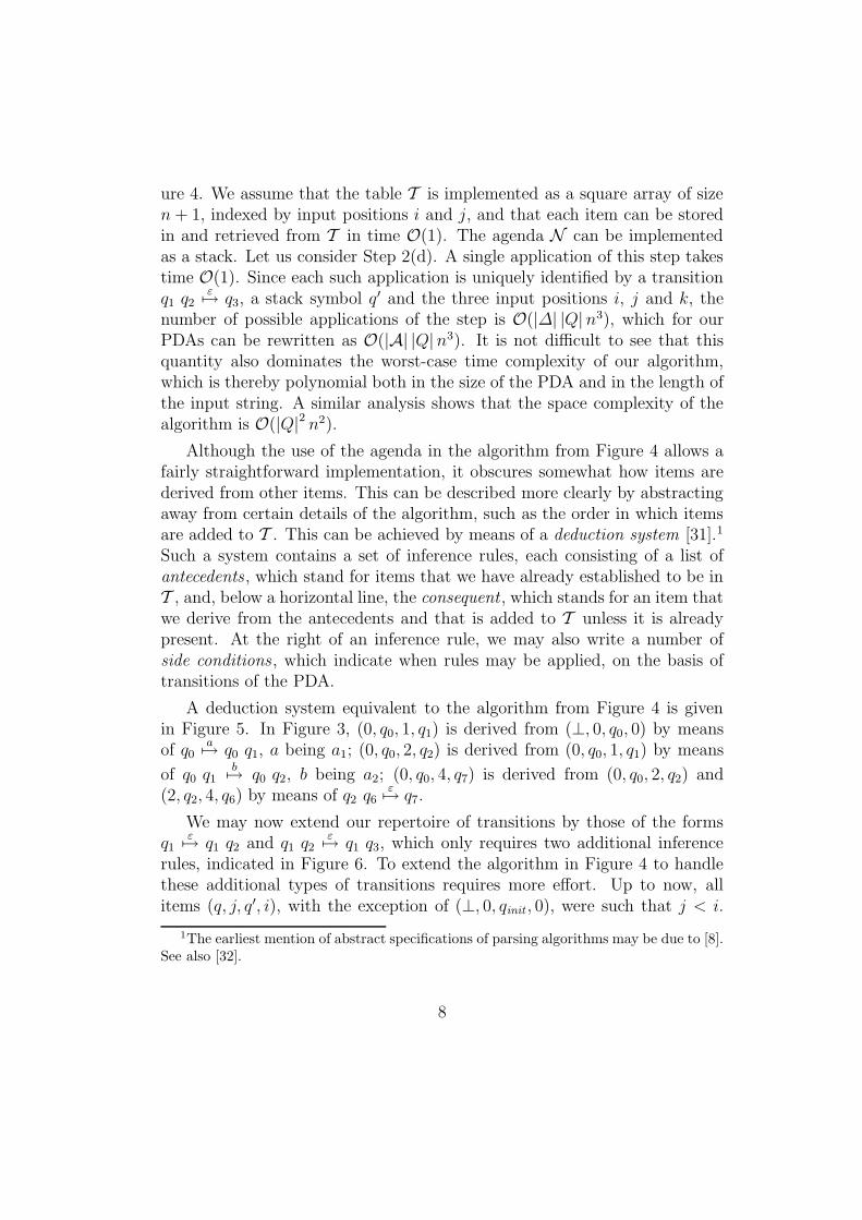
ure 4. We assume that the table T is implemented as a square array of sizen + 1, indexed by input positions i and j, and that each item can be storedin and retrieved from T in time O(1). The agenda N can be implementedas a stack. Let us consider Step 2(d). A single application of this step takestime O(1). Since each such application is uniquely identified by a transitionq1 q2
ε7→ q3, a stack symbol q′ and the three input positions i, j and k, the
number of possible applications of the step is O(|∆| |Q|n3), which for ourPDAs can be rewritten as O(|A| |Q|n3). It is not difficult to see that thisquantity also dominates the worst-case time complexity of our algorithm,which is thereby polynomial both in the size of the PDA and in the length ofthe input string. A similar analysis shows that the space complexity of thealgorithm is O(|Q|2 n2).
Although the use of the agenda in the algorithm from Figure 4 allows afairly straightforward implementation, it obscures somewhat how items arederived from other items. This can be described more clearly by abstractingaway from certain details of the algorithm, such as the order in which itemsare added to T . This can be achieved by means of a deduction system [31].1
Such a system contains a set of inference rules, each consisting of a list ofantecedents, which stand for items that we have already established to be inT , and, below a horizontal line, the consequent , which stands for an item thatwe derive from the antecedents and that is added to T unless it is alreadypresent. At the right of an inference rule, we may also write a number ofside conditions, which indicate when rules may be applied, on the basis oftransitions of the PDA.
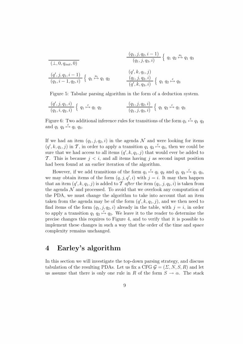
A deduction system equivalent to the algorithm from Figure 4 is givenin Figure 5. In Figure 3, (0, q0, 1, q1) is derived from (⊥, 0, q0, 0) by meansof q0
a7→ q0 q1, a being a1; (0, q0, 2, q2) is derived from (0, q0, 1, q1) by means
of q0 q1b7→ q0 q2, b being a2; (0, q0, 4, q7) is derived from (0, q0, 2, q2) and
(2, q2, 4, q6) by means of q2 q6ε7→ q7.
We may now extend our repertoire of transitions by those of the formsq1
ε7→ q1 q2 and q1 q2
ε7→ q1 q3, which only requires two additional inference
rules, indicated in Figure 6. To extend the algorithm in Figure 4 to handlethese additional types of transitions requires more effort. Up to now, allitems (q, j, q′, i), with the exception of (⊥, 0, qinit , 0), were such that j < i.
1The earliest mention of abstract specifications of parsing algorithms may be due to [8].See also [32].
8
(⊥, 0, qinit , 0)
(q′, j, q1, i − 1)
(q1, i − 1, q2, i)
{
q1ai7→ q1 q2
(q1, j, q2, i − 1)
(q1, j, q3, i)
{
q1 q2ai7→ q1 q3
(q′, k, q1, j)(q1, j, q2, i)
(q′, k, q3, i)
{
q1 q2ε7→ q3
Figure 5: Tabular parsing algorithm in the form of a deduction system.
(q′, j, q1, i)
(q1, i, q2, i)
{
q1ε7→ q1 q2
(q1, j, q2, i)
(q1, j, q3, i)
{
q1 q2ε7→ q1 q3
Figure 6: Two additional inference rules for transitions of the form q1ε7→ q1 q2
and q1 q2ε7→ q1 q3.
If we had an item (q1, j, q2, i) in the agenda N and were looking for items(q′, k, q1, j) in T , in order to apply a transition q1 q2
ε7→ q3, then we could be
sure that we had access to all items (q′, k, q1, j) that would ever be added toT . This is because j < i, and all items having j as second input positionhad been found at an earlier iteration of the algorithm.
However, if we add transitions of the form q1ε7→ q1 q2 and q1 q2
ε7→ q1 q3,
we may obtain items of the form (q, j, q′, i) with j = i. It may then happenthat an item (q′, k, q1, j) is added to T after the item (q1, j, q2, i) is taken fromthe agenda N and processed. To avoid that we overlook any computation ofthe PDA, we must change the algorithm to take into account that an itemtaken from the agenda may be of the form (q′, k, q1, j), and we then need tofind items of the form (q1, j, q2, i) already in the table, with j = i, in orderto apply a transition q1 q2
ε7→ q3. We leave it to the reader to determine the
precise changes this requires to Figure 4, and to verify that it is possible toimplement these changes in such a way that the order of the time and spacecomplexity remains unchanged.
4 Earley’s algorithm
In this section we will investigate the top-down parsing strategy, and discusstabulation of the resulting PDAs. Let us fix a CFG G = (Σ, N, S, R) and letus assume that there is only one rule in R of the form S → α. The stack
9
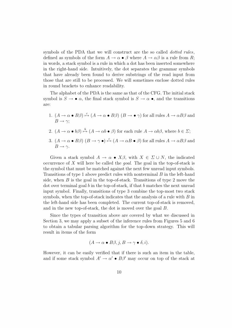
symbols of the PDA that we will construct are the so called dotted rules,defined as symbols of the form A → α • β where A → αβ is a rule from R;in words, a stack symbol is a rule in which a dot has been inserted somewherein the right-hand side. Intuitively, the dot separates the grammar symbolsthat have already been found to derive substrings of the read input fromthose that are still to be processed. We will sometimes enclose dotted rulesin round brackets to enhance readability.
The alphabet of the PDA is the same as that of the CFG. The initial stacksymbol is S → • α, the final stack symbol is S → α •, and the transitionsare:
1. (A → α • Bβ)ε7→ (A → α • Bβ) (B → • γ) for all rules A → αBβ and
B → γ;
2. (A → α • bβ)b7→ (A → αb • β) for each rule A → αbβ, where b ∈ Σ;
3. (A → α • Bβ) (B → γ •)ε7→ (A → αB • β) for all rules A → αBβ and
B → γ.
Given a stack symbol A → α • Xβ, with X ∈ Σ ∪ N , the indicatedoccurrence of X will here be called the goal. The goal in the top-of-stack isthe symbol that must be matched against the next few unread input symbols.Transitions of type 1 above predict rules with nonterminal B in the left-handside, when B is the goal in the top-of-stack. Transitions of type 2 move thedot over terminal goal b in the top-of-stack, if that b matches the next unreadinput symbol. Finally, transitions of type 3 combine the top-most two stacksymbols, when the top-of-stack indicates that the analysis of a rule with B inthe left-hand side has been completed. The current top-of-stack is removed,and in the new top-of-stack, the dot is moved over the goal B.
Since the types of transition above are covered by what we discussed inSection 3, we may apply a subset of the inference rules from Figures 5 and 6to obtain a tabular parsing algorithm for the top-down strategy. This willresult in items of the form
(A → α • Bβ, j, B → γ • δ, i).
However, it can be easily verified that if there is such an item in the table,and if some stack symbol A′ → α′ • Bβ ′ may occur on top of the stack at
10
(0, S → • α, 0)
{
S → α (1)
(j, A → α • Bβ, i)
(i, B → • γ, i)
{
B → γ (2)
(j, A → α • bβ, i − 1)
(j, A → αb • β, i)
{
b = ai (3)
(k, A → α • Bβ, j)(j, B → γ •, i)
(k, A → αB • β, i)(4)
Figure 7: Tabular top-down parsing, or Earley’s algorithm.
position j, then at some point, the table will also contain the item
(A′ → α′ • Bβ ′, j, B → γ • δ, i).
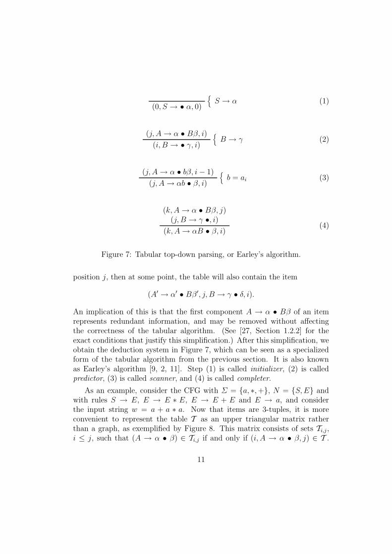
An implication of this is that the first component A → α • Bβ of an itemrepresents redundant information, and may be removed without affectingthe correctness of the tabular algorithm. (See [27, Section 1.2.2] for theexact conditions that justify this simplification.) After this simplification, weobtain the deduction system in Figure 7, which can be seen as a specializedform of the tabular algorithm from the previous section. It is also knownas Earley’s algorithm [9, 2, 11]. Step (1) is called initializer, (2) is calledpredictor, (3) is called scanner, and (4) is called completer.
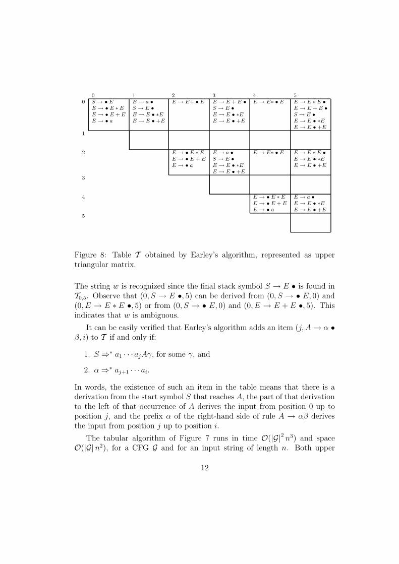
As an example, consider the CFG with Σ = {a, ∗, +}, N = {S, E} andwith rules S → E, E → E ∗ E, E → E + E and E → a, and considerthe input string w = a + a ∗ a. Now that items are 3-tuples, it is moreconvenient to represent the table T as an upper triangular matrix ratherthan a graph, as exemplified by Figure 8. This matrix consists of sets Ti,j,i ≤ j, such that (A → α • β) ∈ Ti,j if and only if (i, A → α • β, j) ∈ T .
11
0 1 2 3 4 50 S → • E
E → • E ∗ E
E → • E + E
E → • a
E → a •
S → E •
E → E • ∗E
E → E • +E
E → E+ • E E → E + E •
S → E •
E → E • ∗E
E → E • +E
E → E∗ • E E → E ∗ E •
E → E + E •
S → E •
E → E • ∗E
E → E • +E
1
2 E → • E ∗ E
E → • E + E
E → • a
E → a •
S → E •
E → E • ∗E
E → E • +E
E → E∗ • E E → E ∗ E •
E → E • ∗E
E → E • +E
3
4 E → • E ∗ E
E → • E + E
E → • a
E → a •
E → E • ∗E
E → E • +E
5
Figure 8: Table T obtained by Earley’s algorithm, represented as uppertriangular matrix.
The string w is recognized since the final stack symbol S → E • is found inT0,5. Observe that (0, S → E •, 5) can be derived from (0, S → • E, 0) and(0, E → E ∗ E •, 5) or from (0, S → • E, 0) and (0, E → E + E •, 5). Thisindicates that w is ambiguous.
It can be easily verified that Earley’s algorithm adds an item (j, A → α •β, i) to T if and only if:
1. S ⇒∗ a1 · · ·ajAγ, for some γ, and
2. α ⇒∗ aj+1 · · ·ai.
In words, the existence of such an item in the table means that there is aderivation from the start symbol S that reaches A, the part of that derivationto the left of that occurrence of A derives the input from position 0 up toposition j, and the prefix α of the right-hand side of rule A → αβ derivesthe input from position j up to position i.
The tabular algorithm of Figure 7 runs in time O(|G|2 n3) and spaceO(|G|n2), for a CFG G and for an input string of length n. Both upper
12
bounds can be easily derived from the general complexity results discussedin Section 3, taking into account the simplification of items to 3-tuples.
To obtain a formulation of Earley’s algorithm closer to a practical imple-mentation, such as that in Figure 4, read the remarks at the end of Section 3concerning the agenda and transitions that read the empty string. Alterna-tively, one may also preprocess certain steps to avoid some of the problemswith the agenda during parse time, as discussed by [12], who also showedthat the worst-case time complexity of Earley’s algorithm can be improvedto O(|G|n3).
5 The Cocke-Kasami-Younger algorithm
Another parsing strategy is (pure) bottom-up parsing, which is also calledshift-reduce parsing [33]. It is particularly simple if the CFG G = (Σ, N, S, R)is in Chomsky normal form, which means that each rule is either of the formA → a, where a ∈ Σ, or of the form A → B C, where B, C ∈ N . The set ofstack symbols is the set of nonterminals of the grammar, and the transitionsare:
1. εa7→ A for each rule A → a;
2. B Cε7→ A for each rule A → B C.
A transition of type 1 consumes the next unread input symbol, and pusheson the stack the nonterminal in the left-hand side of a corresponding rule. Atransition of type 2 can be applied if the top-most two stack symbols B andC are such that B C is the right-hand side of a rule, and it replaces B and Cby the left-hand side A of that rule. Transitions of types 1 and 2 are calledshift and reduce, respectively; see also Section 6. The final stack symbol isS. We deviate from the other sections in this chapter however by assumingthat the PDA starts with an empty stack, or alternatively, that there is someimaginary initial stack symbol that is not in N .
The transitions B Cε7→ A are of a type that we have seen before, and
in a tabular algorithm for the PDA, such transitions can be realized by theinference rule:
13
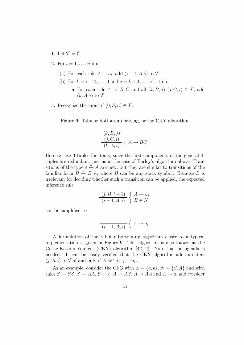
1. Let T = ∅.
2. For i = 1, . . . , n do:
(a) For each rule A → ai, add (i − 1, A, i) to T .
(b) For k = i − 2, . . . , 0 and j = k + 1, . . . , i − 1 do:
• For each rule A → B C and all (k, B, j), (j, C, i) ∈ T , add(k, A, i) to T .
3. Recognize the input if (0, S, n) ∈ T .
Figure 9: Tabular bottom-up parsing, or the CKY algorithm.
(k, B, j)(j, C, i)
(k, A, i)
{
A → BC
Here we use 3-tuples for items, since the first components of the general 4-tuples are redundant, just as in the case of Earley’s algorithm above. Tran-sitions of the type ε
a7→ A are new, but they are similar to transitions of the
familiar form Ba7→ B A, where B can be any stack symbol. Because B is
irrelevant for deciding whether such a transition can be applied, the expectedinference rule
(j, B, i − 1)
(i − 1, A, i)
{
A → ai
B ∈ N
can be simplified to
(i − 1, A, i)
{
A → ai
A formulation of the tabular bottom-up algorithm closer to a typicalimplementation is given in Figure 9. This algorithm is also known as theCocke-Kasami-Younger (CKY) algorithm [42, 2]. Note that no agenda isneeded. It can be easily verified that the CKY algorithm adds an item(j, A, i) to T if and only if A ⇒∗ aj+1 · · ·ai.
As an example, consider the CFG with Σ = {a, b}, N = {S, A} and withrules S → SS, S → AA, S → b, A → AS, A → AA and A → a, and consider
14
1 2 3 40 A S,A S,A S,A
1 A A A
2 S S
3 S
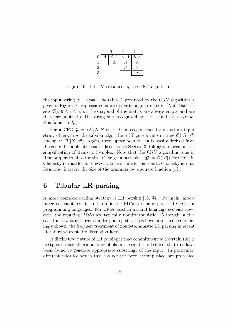
Figure 10: Table T obtained by the CKY algorithm.
the input string w = aabb. The table T produced by the CKY algorithm isgiven in Figure 10, represented as an upper triangular matrix. (Note that thesets Ti,i, 0 ≤ i ≤ n, on the diagonal of the matrix are always empty and aretherefore omitted.) The string w is recognized since the final stack symbolS is found in T0,4.
For a CFG G = (Σ, N, S, R) in Chomsky normal form and an inputstring of length n, the tabular algorithm of Figure 9 runs in time O(|R|n3)and space O(|N |n2). Again, these upper bounds can be easily derived fromthe general complexity results discussed in Section 3, taking into account thesimplification of items to 3-tuples. Note that the CKY algorithm runs intime proportional to the size of the grammar, since |G| = O(|R|) for CFGs inChomsky normal form. However, known transformations to Chomsky normalform may increase the size of the grammar by a square function [13].
6 Tabular LR parsing
A more complex parsing strategy is LR parsing [16, 34]. Its main impor-tance is that it results in deterministic PDAs for many practical CFGs forprogramming languages. For CFGs used in natural language systems how-ever, the resulting PDAs are typically nondeterministic. Although in thiscase the advantages over simpler parsing strategies have never been convinc-ingly shown, the frequent treatment of nondeterministic LR parsing in recentliterature warrants its discussion here.
A distinctive feature of LR parsing is that commitment to a certain rule ispostponed until all grammar symbols in the right-hand side of that rule havebeen found to generate appropriate substrings of the input. In particular,different rules for which this has not yet been accomplished are processed
15
simultaneously, without spending computational effort on any rule individu-ally. As in the case of Earley’s algorithm, we need dotted rules of the formA → α • β, where the dot separates the grammar symbols in the right-handside that have already been found to derive substrings of the read input fromthose that are still to be processed. Whereas in the scanner step (3) and inthe completer step (4) from Earley’s algorithm (Figure 7) each rule is individ-ually processed by letting the dot traverse its right-hand side, in LR parsingthis traversal simultaneously affects sets of dotted rules. Also the equivalentof the predictor step (2) from Earley’s algorithm is now an operation on setsof dotted rules. These operations are pre-compiled into stack symbols andtransitions.
Let us fix a CFG G = (Σ, N, S, R). Assume q is a set of dotted rules. Wedefine closure(q) as the smallest set of dotted rules such that:
1. q ⊆ closure(q), and
2. if (A → α • Bβ) ∈ closure(q) and (B → γ) ∈ R, then (B → • γ) ∈closure(q).
In words, we extend the set of dotted rules by those that can be obtained byrepeatedly applying an operation similar to the predictor step. For a set qof dotted rules and a grammar symbol X ∈ Σ ∪ N , we define:
goto(q, X) = closure({(A → αX • β) | (A → α • Xβ) ∈ q})
The manner in which the dot traverses through right-hand sides can be re-lated to the scanner step of Earley’s algorithm if X ∈ Σ or to the completerstep if X ∈ N .
The initial stack symbol qinit is defined to be closure({(S → • α) | (S →α) ∈ R}); cf. the initializer step (1) of Earley’s algorithm. Other stacksymbols are those non-empty sets of dotted rules that can be derived fromqinit by means of repeated application of the goto function. More precisely,Q is the smallest set such that:
1. qinit ∈ Q, and
2. if q ∈ Q and goto(q, X) = q′ 6= ∅ for some X, then q′ ∈ Q.
For technical reasons, we also need to add a special stack symbol qfinal to Qthat becomes the final stack symbol. The transitions are:
16
1. q1a7→ q1 q2 for all q1, q2 ∈ Q and each a ∈ Σ such that goto(q1, a) = q2;
2. q0 q1 · · · qmε7→ q0 q′ for all q0, . . . , qm, q′ ∈ Q and each (A → α •) ∈ qm
such that |α| = m and q′ = goto(q0, A);
3. q0 q1 · · · qmε7→ qfinal for all q0, . . . , qm ∈ Q and each (S → α •) ∈ qm
such that |α| = m and q0 = qinit .
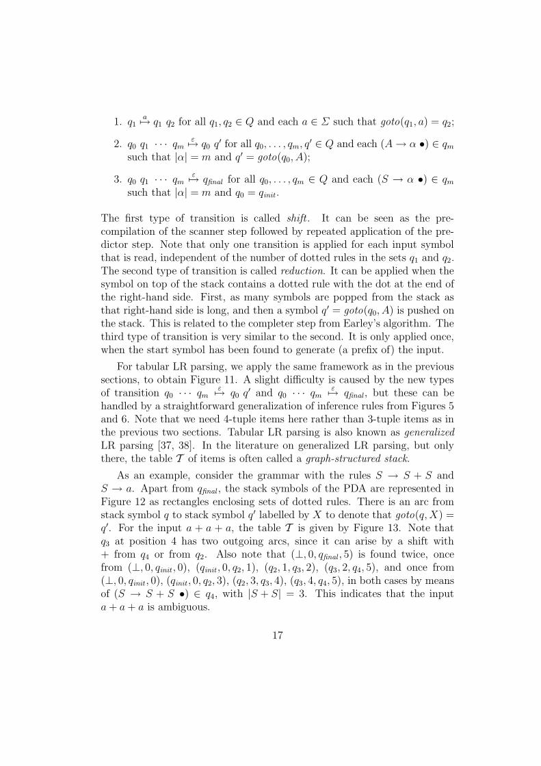
The first type of transition is called shift . It can be seen as the pre-compilation of the scanner step followed by repeated application of the pre-dictor step. Note that only one transition is applied for each input symbolthat is read, independent of the number of dotted rules in the sets q1 and q2.The second type of transition is called reduction. It can be applied when thesymbol on top of the stack contains a dotted rule with the dot at the end ofthe right-hand side. First, as many symbols are popped from the stack asthat right-hand side is long, and then a symbol q′ = goto(q0, A) is pushed onthe stack. This is related to the completer step from Earley’s algorithm. Thethird type of transition is very similar to the second. It is only applied once,when the start symbol has been found to generate (a prefix of) the input.
For tabular LR parsing, we apply the same framework as in the previoussections, to obtain Figure 11. A slight difficulty is caused by the new typesof transition q0 · · · qm
ε7→ q0 q′ and q0 · · · qm
ε7→ qfinal , but these can be
handled by a straightforward generalization of inference rules from Figures 5and 6. Note that we need 4-tuple items here rather than 3-tuple items as inthe previous two sections. Tabular LR parsing is also known as generalizedLR parsing [37, 38]. In the literature on generalized LR parsing, but onlythere, the table T of items is often called a graph-structured stack.
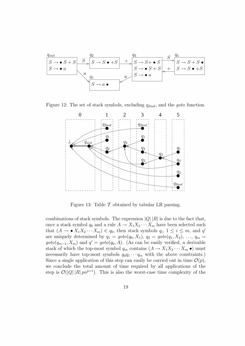
As an example, consider the grammar with the rules S → S + S andS → a. Apart from qfinal , the stack symbols of the PDA are represented inFigure 12 as rectangles enclosing sets of dotted rules. There is an arc fromstack symbol q to stack symbol q′ labelled by X to denote that goto(q, X) =q′. For the input a + a + a, the table T is given by Figure 13. Note thatq3 at position 4 has two outgoing arcs, since it can arise by a shift with+ from q4 or from q2. Also note that (⊥, 0, qfinal , 5) is found twice, oncefrom (⊥, 0, qinit , 0), (qinit , 0, q2, 1), (q2, 1, q3, 2), (q3, 2, q4, 5), and once from(⊥, 0, qinit , 0), (qinit , 0, q2, 3), (q2, 3, q3, 4), (q3, 4, q4, 5), in both cases by meansof (S → S + S •) ∈ q4, with |S + S| = 3. This indicates that the inputa + a + a is ambiguous.
17
(⊥, 0, qinit , 0)(5)
(q′, j, q1, i − 1)
(q1, i − 1, q2, i)
{
goto(q1, ai) = q2 (6)
(q0, j0, q1, j1)(q1, j1, q2, j2)...
(qm−1, jm−1, qm, jm)
(q0, j0, q′, jm)
(A → α •) ∈ qm
|α| = mq′ = goto(q0, A)
(7)
(⊥, 0, q0, j0)(q0, j0, q1, j1)(q1, j1, q2, j2)...
(qm−1, jm−1, qm, jm)
(⊥, 0, qfinal , jm)
(S → α •) ∈ qm
|α| = mq0 = qinit
(8)
Figure 11: Tabular LR parsing, or generalized LR parsing.
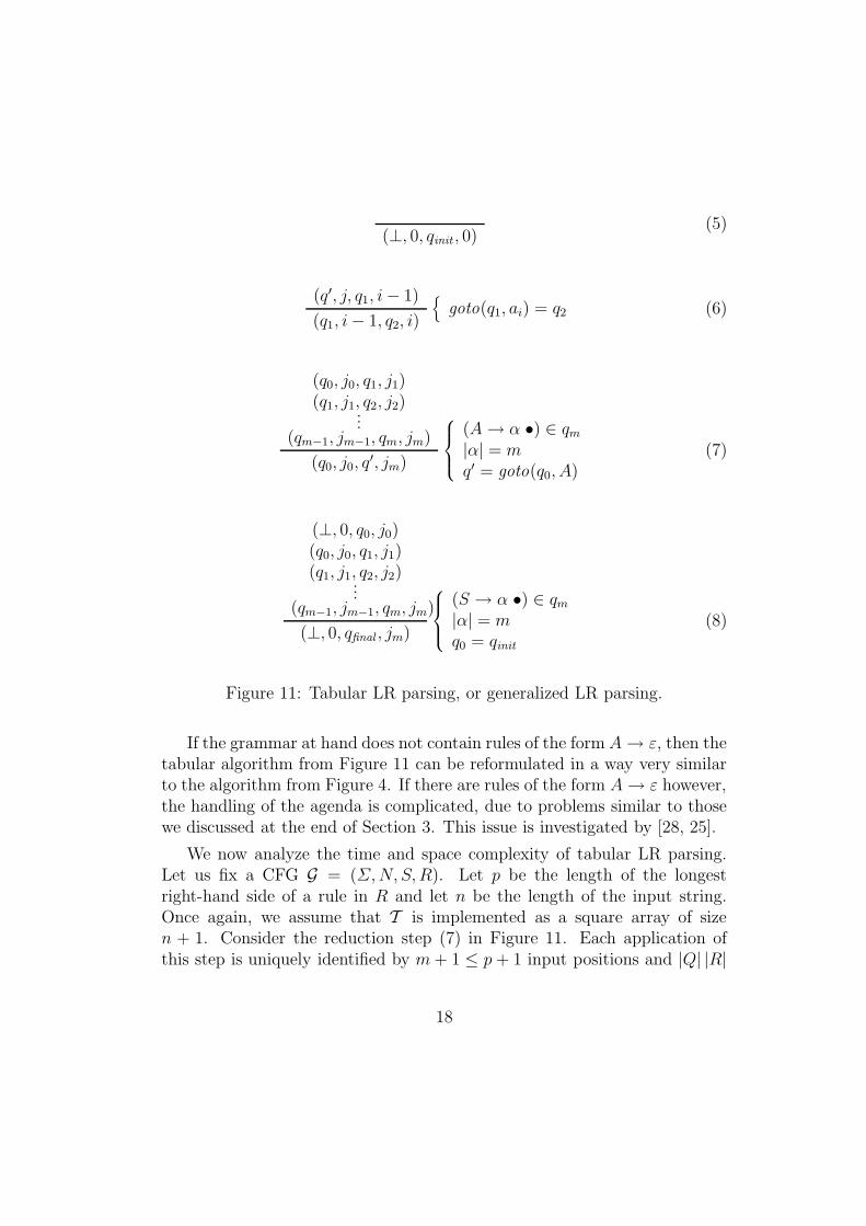
If the grammar at hand does not contain rules of the form A → ε, then thetabular algorithm from Figure 11 can be reformulated in a way very similarto the algorithm from Figure 4. If there are rules of the form A → ε however,the handling of the agenda is complicated, due to problems similar to thosewe discussed at the end of Section 3. This issue is investigated by [28, 25].
We now analyze the time and space complexity of tabular LR parsing.Let us fix a CFG G = (Σ, N, S, R). Let p be the length of the longestright-hand side of a rule in R and let n be the length of the input string.Once again, we assume that T is implemented as a square array of sizen + 1. Consider the reduction step (7) in Figure 11. Each application ofthis step is uniquely identified by m + 1 ≤ p + 1 input positions and |Q| |R|
18
PSfrag replacements
S → • S + S
S → • S + S
S → S • +S
S → S • +S
S → S+ • S S → S + S •S → • a
S → • a
S → a •
SS
aa
+
+
qinit
qfinal
⊥q0
q1
q2 q3 q4
q5
q6
q7
q8
q9
Figure 12: The set of stack symbols, excluding qfinal , and the goto function.
50 4321
PSfrag replacements
S → • S + SS → S • +SS → S+ • SS → S + S •
S → • aS → a •
Sa+
qinit
qfinal qfinal
qfinal
⊥
q0 q1
q1
q1
q2
q2
q2
q3
q3
q4
q4
q5
q6
q7
q8
q9
Figure 13: Table T obtained by tabular LR parsing.
combinations of stack symbols. The expression |Q| |R| is due to the fact that,once a stack symbol q0 and a rule A → X1X2 · · ·Xm have been selected suchthat (A → • X1X2 · · ·Xm) ∈ q0, then stack symbols qi, 1 ≤ i ≤ m, and q′
are uniquely determined by q1 = goto(q0, X1), q2 = goto(q1, X2), . . ., qm =goto(qm−1, Xm) and q′ = goto(q0, A). (As can be easily verified, a derivablestack of which the top-most symbol qm contains (A → X1X2 · · ·Xm •) mustnecessarily have top-most symbols q0q1 · · · qm with the above constraints.)Since a single application of this step can easily be carried out in time O(p),we conclude the total amount of time required by all applications of thestep is O(|Q| |R| pnp+1). This is also the worst-case time complexity of the
19
algorithm, since the running time is dominated by the reduction step (7).From the general complexity results discussed in Section 3 it follows that theworst-case space complexity is O(|Q|2 n2).
We observe that while the above time bound is polynomial in the lengthof the input string, it can be much worse than the corresponding boundsfor Earley’s algorithm or for the CKY algorithm, since p is not bounded.A solution to this problem has been discussed by [15, 26] and consists insplitting each reduction into O(p) transitions of the form q ′q′′
ε7→ q. In
this way, the maximum length of transitions becomes independent of thegrammar. This results in tabular implementations of LR parsing with cubictime complexity in the length of the input. We furthermore observe that theterm |Q| in the above bounds depends on the specific structure of G, andmay grow exponentially with |G| [34, Proposition 6.46].
7 Parse trees
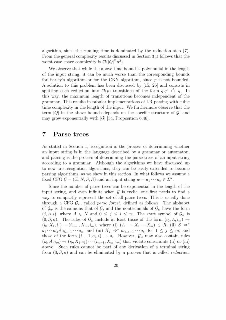
As stated in Section 1, recognition is the process of determining whetheran input string is in the language described by a grammar or automaton,and parsing is the process of determining the parse trees of an input stringaccording to a grammar. Although the algorithms we have discussed upto now are recognition algorithms, they can be easily extended to becomeparsing algorithms, as we show in this section. In what follows we assume afixed CFG G = (Σ, N, S, R) and an input string w = a1 · · ·an ∈ Σ∗.
Since the number of parse trees can be exponential in the length of theinput string, and even infinite when G is cyclic, one first needs to find away to compactly represent the set of all parse trees. This is usually donethrough a CFG Gw, called parse forest , defined as follows. The alphabetof Gw is the same as that of G, and the nonterminals of Gw have the form(j, A, i), where A ∈ N and 0 ≤ j ≤ i ≤ n. The start symbol of Gw is(0, S, n). The rules of Gw include at least those of the form (i0, A, im) →(i0, X1, i1) · · · (im−1, Xm, im), where (i) (A → X1 · · ·Xm) ∈ R, (ii) S ⇒∗
a1 · · ·ai0Aaim+1 · · ·an, and (iii) Xj ⇒∗ aij−1+1 · · ·aij for 1 ≤ j ≤ m, andthose of the form (i − 1, ai, i) → ai. However, Gw may also contain rules(i0, A, im) → (i0, X1, i1) · · · (im−1, Xm, im) that violate constraints (ii) or (iii)above. Such rules cannot be part of any derivation of a terminal stringfrom (0, S, n) and can be eliminated by a process that is called reduction.
20
Reduction can be carried out in linear time in the size of Gw [33].
It is not difficult to show that the parse forest Gw generates a finite lan-guage, which is either {w} if w is in the language generated by G, or ∅otherwise. Furthermore, there is a one-to-one correspondence between parsetrees according to Gw and parse trees of w according to G, with correspondingparse trees being isomorphic.
To give a concrete example, let us consider the CKY algorithm presentedin Section 5. In order to extend this recognition algorithm to a parsing algo-rithm, we may construct the parse forest Gw with rules of the form (j, A, i) →(j, B, k) (k, C, i), where (A → B C) ∈ R and (j, B, k), (k, C, i) ∈ T , rules ofthe form (i − 1, A, i) → (i − 1, ai, i), where (A → ai) ∈ R, and rules of theform (i − 1, ai, i) → ai. Such rules can be constructed during the computa-tion of the table T . In order to perform reduction on Gw, one may visit thenonterminals of Gw starting from (0, S, n), following the rules in a top-downfashion, eliminating the nonterminals and the associated rules that are neverreached. From the resulting parse forest Gw, individual parse trees can beextracted in time proportional to the size of the parse tree itself, which inthe case of CFGs in Chomsky normal form is O(n). One may also extractparse trees directly from table T , but the time complexity then becomesO(|G|n2) [2, 11].
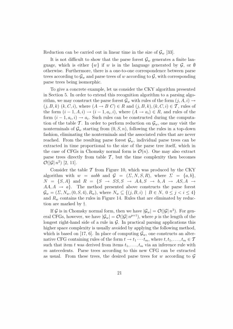
Consider the table T from Figure 10, which was produced by the CKYalgorithm with w = aabb and G = (Σ, N, S, R), where Σ = {a, b},N = {S, A} and R = {S → SS, S → AA, S → b, A → AS, A →AA, A → a}. The method presented above constructs the parse forestGw = (Σ, Nw, (0, S, 4), Rw), where Nw ⊆ {(j, B, i) | B ∈ N, 0 ≤ j < i ≤ 4}and Rw contains the rules in Figure 14. Rules that are eliminated by reduc-tion are marked by †.
If G is in Chomsky normal form, then we have |Gw| = O(|G|n3). For gen-eral CFGs, however, we have |Gw| = O(|G|np+1), where p is the length of thelongest right-hand side of a rule in G. In practical parsing applications thishigher space complexity is usually avoided by applying the following method,which is based on [17, 6]. In place of computing Gw, one constructs an alter-native CFG containing rules of the form t → t1 · · · tm, where t, t1, . . . , tm ∈ Tsuch that item t was derived from items t1, . . . , tm via an inference rule withm antecedents. Parse trees according to this new CFG can be extractedas usual. From these trees, the desired parse trees for w according to G
21
(0, a, 1) → a(1, a, 2) → a(2, b, 3) → b(3, b, 4) → b(0, A, 1) → (0, a, 1)(1, A, 2) → (1, a, 2)(2, S, 3) → (2, b, 3)(3, S, 4) → (3, b, 4)
(0, S, 2) → (0, A, 1) (1, A, 2)
(0, A, 2) → (0, A, 1) (1, A, 2) †
(1, A, 3) → (1, A, 2) (2, S, 3)
(2, S, 4) → (2, S, 3) (3, S, 4)
(0, S, 3) → (0, A, 1) (1, A, 3)(0, S, 3) → (0, S, 2) (2, S, 3)
(0, A, 3) → (0, A, 1) (1, A, 3) †(0, A, 3) → (0, A, 2) (2, S, 3) †
(1, A, 4) → (1, A, 2) (2, S, 4)(1, A, 4) → (1, A, 3) (3, S, 4)
(0, S, 4) → (0, A, 1) (1, A, 4)(0, S, 4) → (0, S, 2) (2, S, 4)(0, S, 4) → (0, S, 3) (3, S, 4)
(0, A, 4) → (0, A, 1) (1, A, 4) †(0, A, 4) → (0, A, 2) (2, S, 4) †(0, A, 4) → (0, A, 3) (3, S, 4) †
Figure 14: Parse forest associated with table T from Figure 10.
can be easily obtained by elementary tree editing operations such as noderelabelling and node erasing. The precise editing algorithm that should beapplied depends on the deduction system underlying the adopted recognitionalgorithm.
If the adopted recognition algorithm has inference rules with no morethan m = 2 antecedents, then the space complexity of the parsing methoddiscussed above, expressed as a function of the length n of the input string,is O(n3). Note that m = 2 in the case of Earley’s algorithm, and this alsoholds in practical implementations of tabular LR parsing, as discussed atthe end of Section 6. The space complexity in the size of G may be largerthan O(|G|), however; it is O(|G|2) in the case of Earley’s algorithm and evenexponential in the case of tabular LR parsing.
The parse forest representation is originally due to [5], with states ofa finite automaton in place of positions in an input string. Parse forestshave also been discussed by [7, 30, 37, 22]. Similar ideas were proposed fortree-adjoining grammars by [40, 18] (see [14] and references therein for thedefinition of tree-adjoining grammars).
22
8 Further references
In this chapter we have restricted ourselves to tabulation for context-freeparsing, on the basis of PDAs. A similar kind of tabulation was also de-veloped for tree-adjoining grammars on the basis of an extended type ofPDA [3]. Tabulation for an even more general type of PDA was discussedby [41].
A further restriction we have made is that the input to the parser must bea string. Context-free parsing can however be generalized to input consistingof a finite automaton. Finite automata without cycles used in speech recog-nition systems are also referred to as word graphs or word lattices [4]. Theparsing methods developed in this chapter can be easily adapted to parsingof finite automata, by manipulating states of an input automaton in place ofpositions in an input string. This technique can be traced back to [5], whichwe mentioned before in Section 7.
PDAs are usually considered to read input from left to right, and theforms of tabulation that we discussed follow that directionality.2 For typesof tabular parsing that are not strictly in one direction, such as head-drivenparsing [32] and island-driven parsing [29], it is less appealing to take PDAsas starting point.
Earley’s algorithm and the CKY algorithm run in cubic time in the lengthof the input string. An asymptotically faster method for context-free parsinghas been developed by [39], using a reduction from context-free recognitionto Boolean matrix multiplication. An inverse reduction from Boolean matrixmultiplication to context-free recognition has been presented by [20], provid-ing evidence that asymptotically faster methods for context-free recognitionmight not be of practical interest.
The extension of tabular parsing with weights or probabilities has beenconsidered by [23] for Earley’s algorithm, by [35] for the CKY algorithm, andby [19] for tabular LR parsing. Deduction systems for parsing extended withweights are discussed by [10].
2There are alternative forms of tabulation that do not adopt the left-to-right mode ofprocessing from the PDA [1, 24].
23
References
[1] A.V. Aho, J.E. Hopcroft, and J.D. Ullman. Time and tape complexity ofpushdown automaton languages. Information and Control, 13:186–206,1968.
[2] A.V. Aho and J.D. Ullman. Parsing, volume 1 of The Theory of Parsing,Translation and Compiling. Prentice-Hall, 1972.
[3] M. A. Alonso Pardo, M.-J. Nederhof, and E. Villemonte de la Clergerie.Tabulation of automata for tree-adjoining languages. Grammars, 3:89–110, 2000.
[4] H. Aust, M. Oerder, F. Seide, and V. Steinbiss. The Philips automatictrain timetable information system. Speech Communication, 17:249–262,1995.
[5] Y. Bar-Hillel, M. Perles, and E. Shamir. On formal properties of simplephrase structure grammars. In Y. Bar-Hillel, editor, Language and In-formation: Selected Essays on their Theory and Application, chapter 9,pages 116–150. Addison-Wesley, 1964.
[6] S. Billot and B. Lang. The structure of shared forests in ambiguousparsing. In 27th Annual Meeting of the Association for ComputationalLinguistics, Proceedings of the Conference, pages 143–151, Vancouver,British Columbia, Canada, June 1989.
[7] J. Cocke and J.T. Schwartz. Programming Languages and Their Com-pilers — Preliminary Notes, pages 184–206. Courant Institute of Math-ematical Sciences, New York University, second revised version, April1970.
[8] S.A. Cook. Path systems and language recognition. In ACM Symposiumon Theory of Computing, pages 70–72, 1970.
[9] J. Earley. An efficient context-free parsing algorithm. Communicationsof the ACM, 13(2):94–102, February 1970.
[10] J. Goodman. Semiring parsing. Computational Linguistics, 25(4):573–605, 1999.
24
[11] S.L. Graham and M.A. Harrison. Parsing of general context free lan-guages. In Advances in Computers, volume 14, pages 77–185. AcademicPress, New York, NY, 1976.
[12] S.L. Graham, M.A. Harrison, and W.L. Ruzzo. An improved context-free recognizer. ACM Transactions on Programming Languages and Sys-tems, 2(3):415–462, July 1980.
[13] M.A. Harrison. Introduction to Formal Language Theory. Addison-Wesley, 1978.
[14] A.K. Joshi and Y. Schabes. Tree-adjoining grammars. In G. Rozen-berg and A. Salomaa, editors, Handbook of Formal Languages.Vol 3: Beyond Words, chapter 2, pages 69–123. Springer-Verlag,Berlin/Heidelberg/New York, 1997.
[15] J.R. Kipps. GLR parsing in time O(n3). In M. Tomita, editor, General-ized LR Parsing, chapter 4, pages 43–59. Kluwer Academic Publishers,1991.
[16] D.E. Knuth. On the translation of languages from left to right. Infor-mation and Control, 8:607–639, 1965.
[17] B. Lang. Deterministic techniques for efficient non-deterministic parsers.In Automata, Languages and Programming, 2nd Colloquium, volume 14of Lecture Notes in Computer Science, pages 255–269, Saarbrucken,1974. Springer-Verlag.
[18] B. Lang. Recognition can be harder than parsing. Computational Intel-ligence, 10(4):486–494, 1994.
[19] A. Lavie and M. Tomita. GLR∗ – an efficient noise-skipping parsingalgorithm for context free grammars. In Third International Workshopon Parsing Technologies, pages 123–134, Tilburg (The Netherlands) andDurbuy (Belgium), August 1993.
[20] L. Lee. Fast context-free grammar parsing requires fast boolean matrixmultiplication. Journal of the ACM, 49(1):1–15, 2001.
[21] R. Leermakers. The Functional Treatment of Parsing. Kluwer AcademicPublishers, 1993.
25
[22] H. Leiss. On Kilbury’s modification of Earley’s algorithm. ACM Trans-actions on Programming Languages and Systems, 12(4):610–640, Octo-ber 1990.
[23] G. Lyon. Syntax-directed least-errors analysis for context-free languages:A practical approach. Communications of the ACM, 17(1):3–14, January1974.
[24] M.-J. Nederhof. Reversible pushdown automata and bidirectional pars-ing. In J. Dassow, G. Rozenberg, and A. Salomaa, editors, Developmentsin Language Theory II, pages 472–481. World Scientific, Singapore, 1996.
[25] M.-J. Nederhof and J.J. Sarbo. Increasing the applicability of LR pars-ing. In H. Bunt and M. Tomita, editors, Recent Advances in ParsingTechnology, chapter 3, pages 35–57. Kluwer Academic Publishers, 1996.
[26] M.-J. Nederhof and G. Satta. Efficient tabular LR parsing. In 34thAnnual Meeting of the Association for Computational Linguistics, Pro-ceedings of the Conference, pages 239–246, Santa Cruz, California, USA,June 1996.
[27] M.J. Nederhof. Linguistic Parsing and Program Transformations. PhDthesis, University of Nijmegen, 1994.
[28] R. Nozohoor-Farshi. GLR parsing for ε-grammars. In M. Tomita, edi-tor, Generalized LR Parsing, chapter 5, pages 61–75. Kluwer AcademicPublishers, 1991.
[29] G. Satta and O. Stock. Bidirectional context-free grammar parsing fornatural language processing. Artificial Intelligence, 69:123–164, 1994.
[30] B.A. Sheil. Observations on context-free parsing. Statistical Methods inLinguistics, pages 71–109, 1976.
[31] S.M. Shieber, Y. Schabes, and F.C.N. Pereira. Principles and imple-mentation of deductive parsing. Journal of Logic Programming, 24:3–36,1995.
[32] K. Sikkel. Parsing Schemata. Springer-Verlag, 1997.
26
[33] S. Sippu and E. Soisalon-Soininen. Parsing Theory, Vol. I: Languagesand Parsing, volume 15 of EATCS Monographs on Theoretical ComputerScience. Springer-Verlag, 1988.
[34] S. Sippu and E. Soisalon-Soininen. Parsing Theory, Vol. II: LR(k) andLL(k) Parsing, volume 20 of EATCS Monographs on Theoretical Com-puter Science. Springer-Verlag, 1990.
[35] R. Teitelbaum. Context-free error analysis by evaluation of algebraicpower series. In Conference Record of the Fifth Annual ACM Symposiumon Theory of Computing, pages 196–199, 1973.
[36] H. Thompson and G. Ritchie. Implementing natural language parsers.In T. O’Shea and M. Eisenstadt, editors, Artificial Intelligence: Tools,Techniques, and Applications, chapter 9, pages 245–300. Harper & Row,New York, 1984.
[37] M. Tomita. Efficient Parsing for Natural Language. Kluwer AcademicPublishers, 1986.
[38] M. Tomita. An efficient augmented-context-free parsing algorithm.Computational Linguistics, 13:31–46, 1987.
[39] L.G. Valiant. General context-free recognition in less than cubic time.Journal of Computer and System Sciences, 10:308–315, 1975.
[40] K. Vijay-Shanker and D.J. Weir. The use of shared forests in tree adjoin-ing grammar parsing. In Sixth Conference of the European Chapter ofthe Association for Computational Linguistics, Proceedings of the Con-ference, pages 384–393, Utrecht, The Netherlands, April 1993.
[41] E. Villemonte de la Clergerie and F. Barthelemy. Information flow intabular interpretations for generalized push-down automata. TheoreticalComputer Science, 199:167–198, 1998.
[42] D.H. Younger. Recognition and parsing of context-free languages in timen3. Information and Control, 10:189–208, 1967.
27
1
Tabular Parsing
Giorgio SattaUniversity of Padua
http://www.dei.unipd.it/~satta/
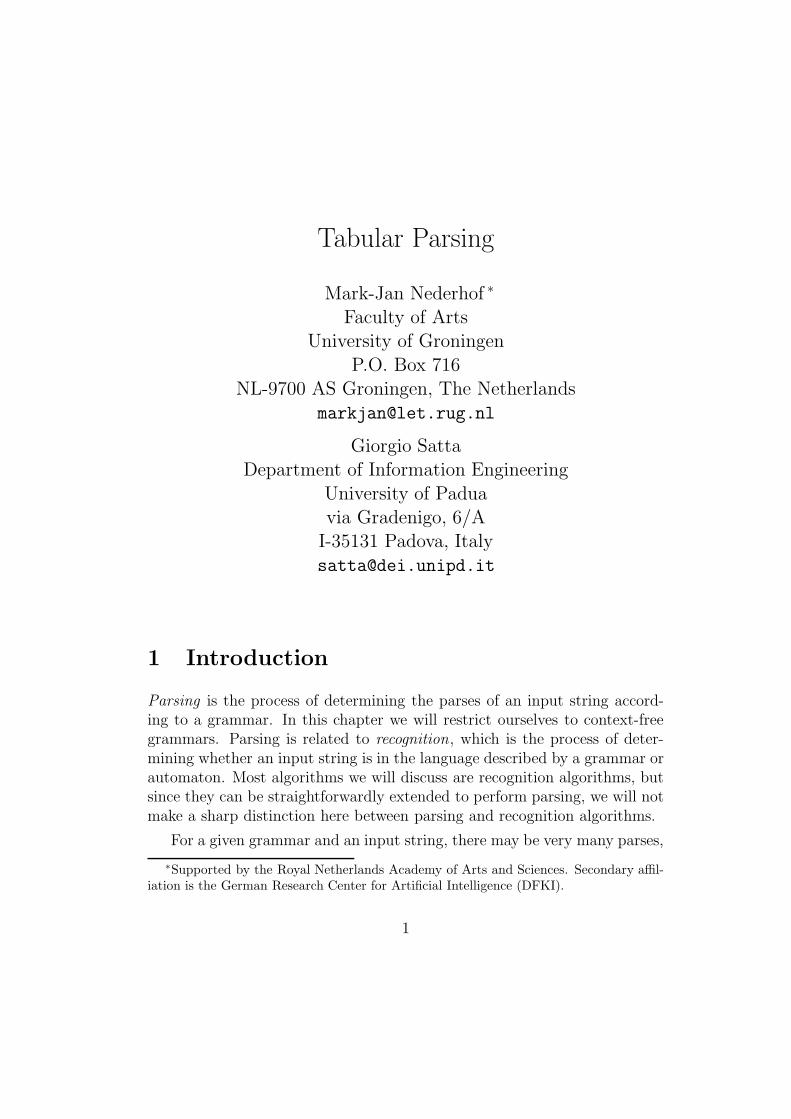
ESSLLI 2004 Tabular Parsing 2
Introduction
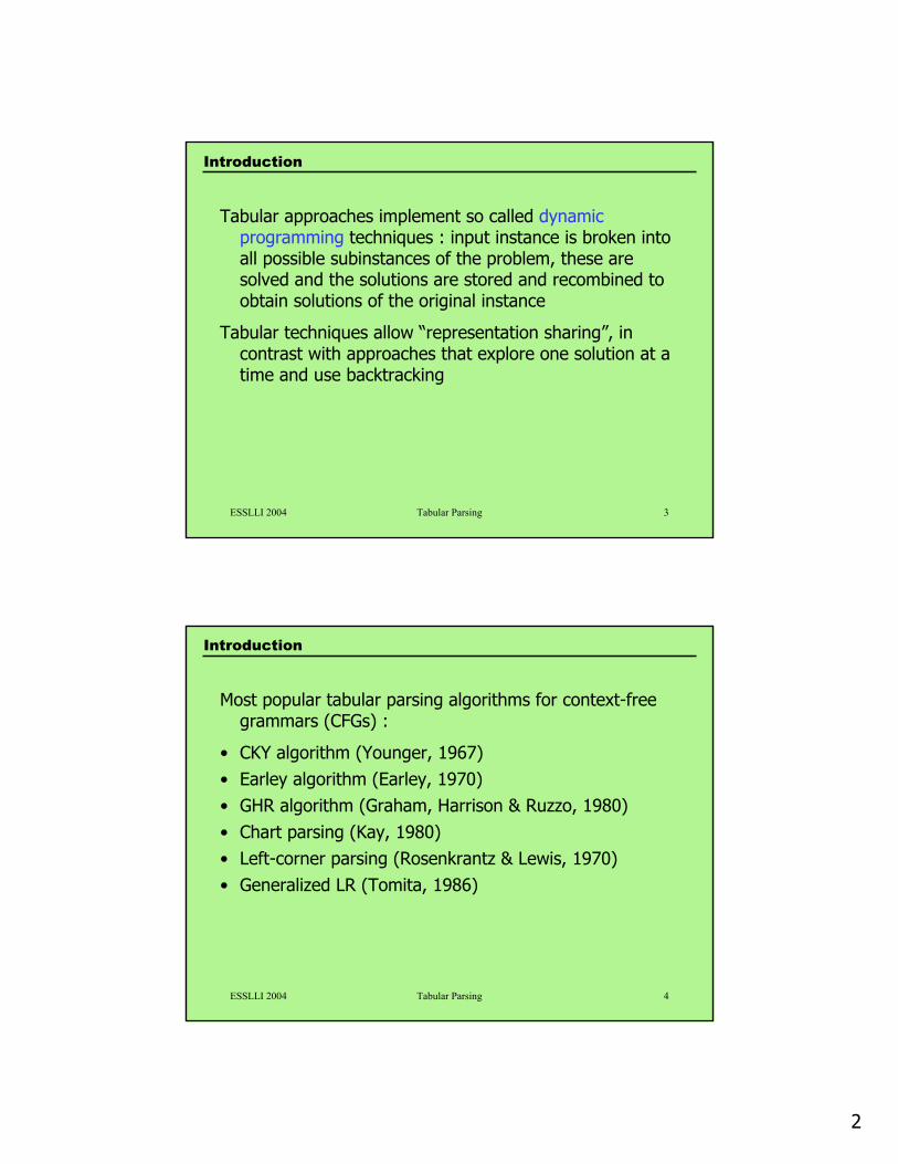
Parsing : retrieving all derivations/trees assigned by input grammar G to input string w
Recognition : detecting whether input grammar Ggenerates string w
Recognition and Parsing algorithms are closely related
2
ESSLLI 2004 Tabular Parsing 3
Introduction
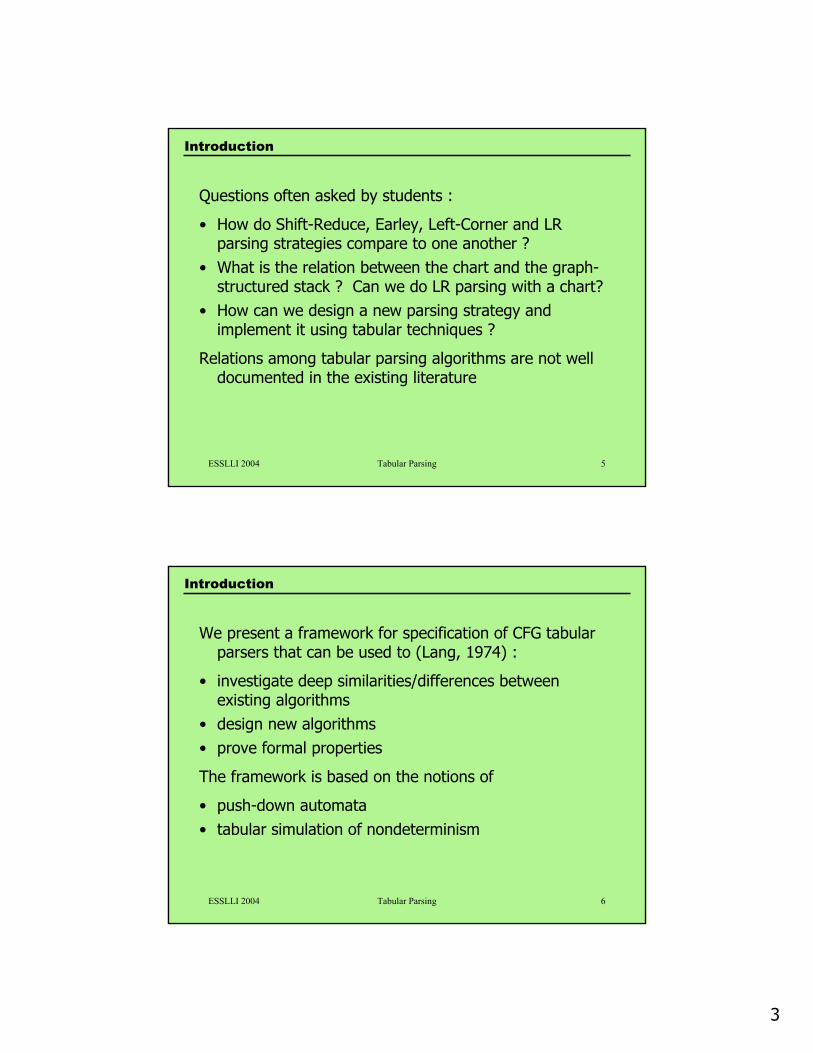
Tabular approaches implement so called dynamic programming techniques : input instance is broken into all possible subinstances of the problem, these are solved and the solutions are stored and recombined to obtain solutions of the original instance
Tabular techniques allow “representation sharing”, in contrast with approaches that explore one solution at a time and use backtracking
ESSLLI 2004 Tabular Parsing 4
Introduction
Most popular tabular parsing algorithms for context-free grammars (CFGs) :
• CKY algorithm (Younger, 1967)• Earley algorithm (Earley, 1970)• GHR algorithm (Graham, Harrison & Ruzzo, 1980)• Chart parsing (Kay, 1980)• Left-corner parsing (Rosenkrantz & Lewis, 1970)• Generalized LR (Tomita, 1986)
3
ESSLLI 2004 Tabular Parsing 5
Introduction
Questions often asked by students :
• How do Shift-Reduce, Earley, Left-Corner and LR parsing strategies compare to one another ?
• What is the relation between the chart and the graph-structured stack ? Can we do LR parsing with a chart?
• How can we design a new parsing strategy and implement it using tabular techniques ?
Relations among tabular parsing algorithms are not well documented in the existing literature
ESSLLI 2004 Tabular Parsing 6
Introduction
We present a framework for specification of CFG tabular parsers that can be used to (Lang, 1974) :
• investigate deep similarities/differences between existing algorithms
• design new algorithms• prove formal properties
The framework is based on the notions of
• push-down automata• tabular simulation of nondeterminism
4
ESSLLI 2004 Tabular Parsing 7
Introduction
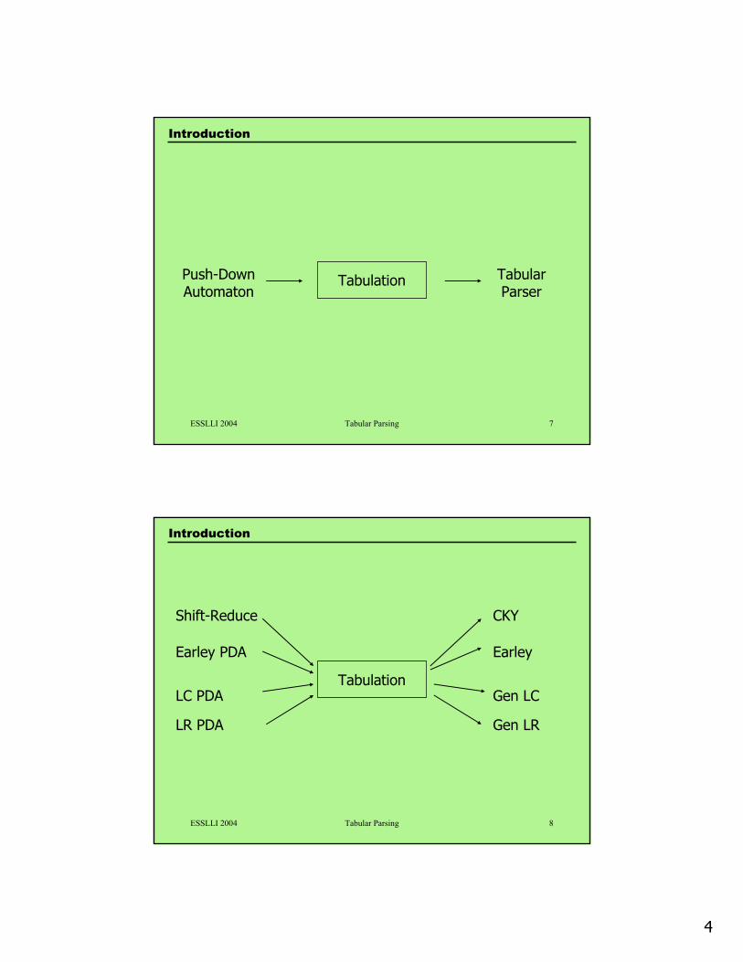
TabulationPush-Down Automaton
Tabular Parser
ESSLLI 2004 Tabular Parsing 8
Introduction
Tabulation
Shift-Reduce
LC PDA
Earley PDA
LR PDA
Earley
CKY
Gen LC
Gen LR
5
ESSLLI 2004 Tabular Parsing 9
Formal Background
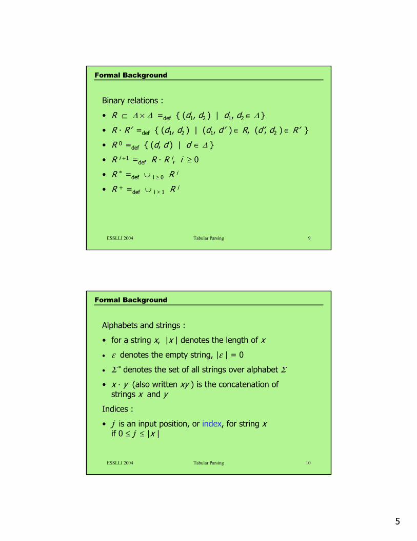
Binary relations :
• R ⊆ ∆ × ∆ =def { (d1, d2 ) | d1, d2 ∈ ∆ }
• R · R’ =def { (d1, d2 ) | (d1, d’ ) ∈ R, (d’, d2 ) ∈ R’ }
• R 0 =def { (d, d ) | d ∈ ∆ }
• R i +1 =def R · R i, i ≥ 0
• R * =def ∪ i ≥ 0 R i
• R + =def ∪ i ≥ 1 R i
ESSLLI 2004 Tabular Parsing 10
Formal Background
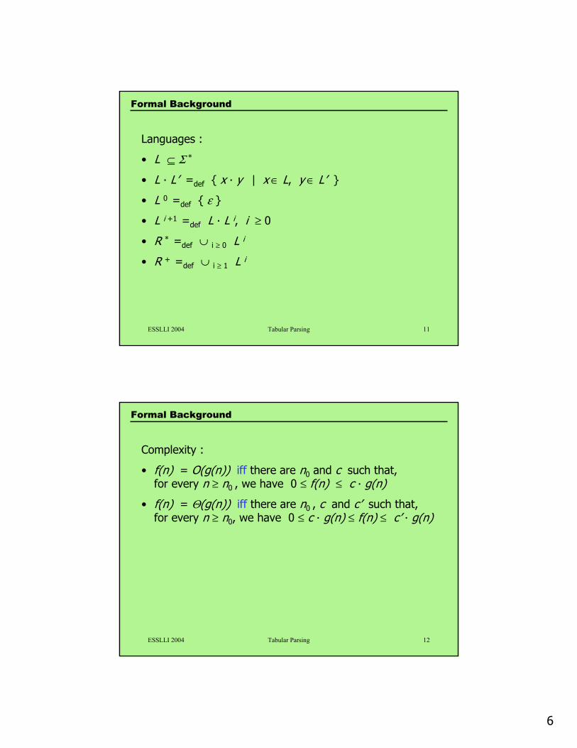
Alphabets and strings :
• for a string x, |x | denotes the length of x
• ε denotes the empty string, |ε | = 0
• Σ * denotes the set of all strings over alphabet Σ
• x · y (also written xy ) is the concatenation of strings x and y
Indices :
• j is an input position, or index, for string xif 0 ≤ j ≤ |x |
6
ESSLLI 2004 Tabular Parsing 11
Formal Background
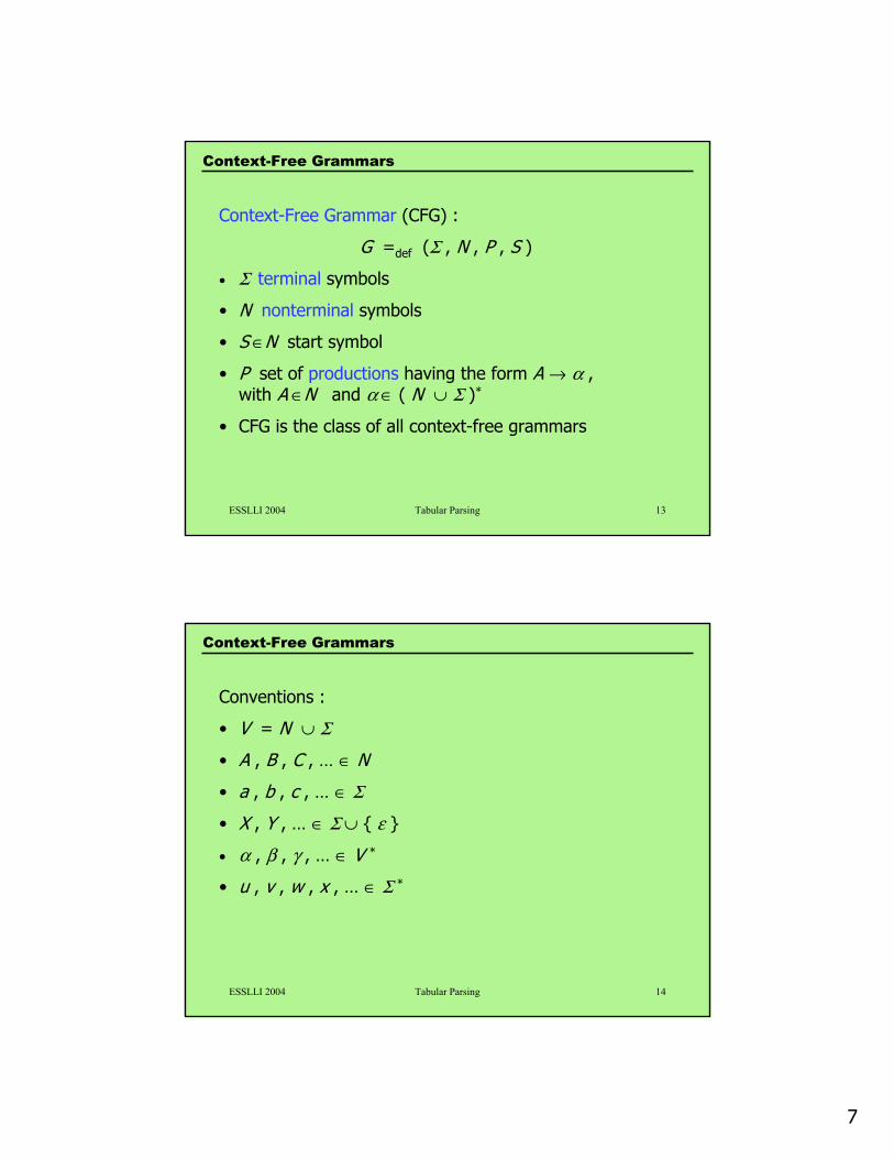
Languages :
• L ⊆ Σ *
• L · L’ =def { x · y | x ∈ L, y ∈ L’ }
• L 0 =def { ε }
• L i +1 =def L · L i, i ≥ 0
• R * =def ∪ i ≥ 0 L i
• R + =def ∪ i ≥ 1 L i
ESSLLI 2004 Tabular Parsing 12
Complexity :
• f(n) = O(g(n)) iff there are n0 and c such that, for every n ≥ n0 , we have 0 ≤ f(n) ≤ c · g(n)
• f(n) = Θ(g(n)) iff there are n0 , c and c’ such that, for every n ≥ n0, we have 0 ≤ c · g(n) ≤ f(n) ≤ c’ · g(n)
Formal Background
7
ESSLLI 2004 Tabular Parsing 13
Context-Free Grammars
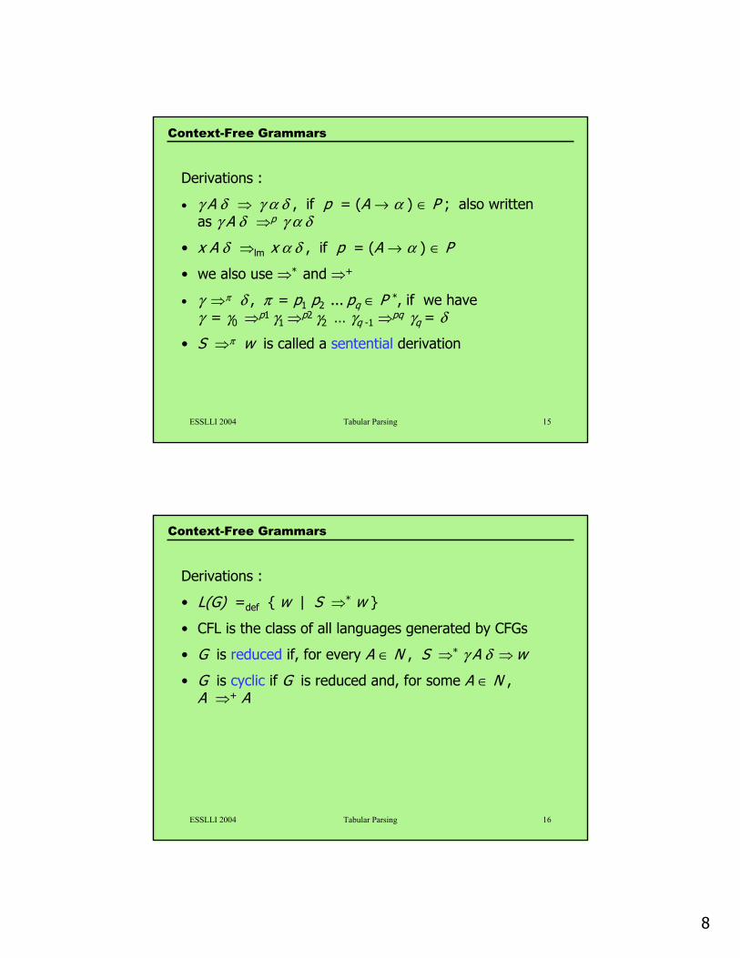
Context-Free Grammar (CFG) :
G =def (Σ , N , P , S )
• Σ terminal symbols
• N nonterminal symbols
• S ∈N start symbol
• P set of productions having the form A → α , with A ∈N and α ∈ ( N ∪ Σ )*
• CFG is the class of all context-free grammars
ESSLLI 2004 Tabular Parsing 14
Context-Free Grammars
Conventions :
• V = N ∪ Σ
• A , B , C , … ∈ N
• a , b , c , … ∈ Σ
• X , Y , … ∈ Σ ∪ { ε }
• α , β , γ , … ∈ V *
• u , v , w , x , … ∈ Σ *
8
ESSLLI 2004 Tabular Parsing 15
Context-Free Grammars
Derivations :
• γ A δ ⇒ γ α δ , if p = (A → α ) ∈ P ; also written as γ A δ ⇒p γ α δ
• x A δ ⇒lm x α δ , if p = (A → α ) ∈ P
• we also use ⇒* and ⇒+
• γ ⇒π δ , π = p1 p2 ... pq ∈ P *, if we have γ = γ0 ⇒p1 γ1 ⇒p2 γ2 … γq -1 ⇒pq γq = δ
• S ⇒π w is called a sentential derivation
ESSLLI 2004 Tabular Parsing 16
Context-Free Grammars
Derivations :
• L(G) =def { w | S ⇒* w }
• CFL is the class of all languages generated by CFGs
• G is reduced if, for every A ∈ N , S ⇒* γ A δ ⇒w
• G is cyclic if G is reduced and, for some A ∈ N , A ⇒+ A
9
ESSLLI 2004 Tabular Parsing 17
Context-Free Grammars
Parse trees :
• sentential derivations can be described by means of labeled, ordered trees called parse trees
• parse trees do not represent the order of rule application, but represent the nonterminal that is rewritten by each rule
ESSLLI 2004 Tabular Parsing 18
Context-Free Grammars
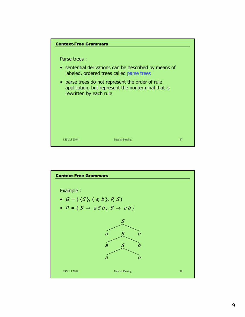
Example :
• G = ( {S }, { a, b }, P, S )
• P = { S → a S b , S → a b }
S
b a S
b a S
b a
10
ESSLLI 2004 Tabular Parsing 19
Context-Free Grammars
Parse trees :
• T(G) =def set of all parse trees for G
• T(G, w) =def set of all parse trees for G with yield w
ESSLLI 2004 Tabular Parsing 20
Context-Free Grammars
Ambiguity :
• G is unambiguous if, for every w ∈ L(G) we have |T(G, w) | = 1
• G is ambiguous if it is not unambiguous
• L ∈ CFL is ambiguous if there is no CFG G such that L(G) = L and G is unambiguous
11
ESSLLI 2004 Tabular Parsing 21
Context-Free Grammars
Ambiguity :
• d(n) =def max|w | = n |T(G, w) |
• G is massively ambiguous if there is no polynomial p(n) such that d(n) = O(p(n))
• G is infinitely ambiguous if, for some w, T(G, w) is an infinite set
ESSLLI 2004 Tabular Parsing 22
Context-Free Grammars
Example :
• G = ( {S }, { a }, P, S )
• P = { S → S S , S → a }
• G is massively ambiguous, generating all possible binary bracketings for a string
• d(n) is the series of Catalan numbers
12
ESSLLI 2004 Tabular Parsing 23
Context-Free Grammars
Example :
• G = (Σ , N , P , S )
• N = { S, VP, NP, PP, V, N, P, Det }
• Σ = { eat, I, chocolate, fork, strawberries, with, a }
• P = { NP → NP PP | Det N | N ,VP → VP PP | V NP , PP → P NP , N → chocolate | I | fork | strawberries, V → eat , Det → a , P → with }
ESSLLI 2004 Tabular Parsing 24
Context-Free Grammars
Example :
• I eat [NP [NP chocolate ] [PP with strawberries ] ]
• I [VP [VP eat [NP chocolate ] ] [PP with a fork ] ]
• *I [VP [VP eat [NP chocolate ] ] [PP with strawberries ] ]
• *I eat [NP [NP chocolate ] [PP with a fork ] ]
13
ESSLLI 2004 Tabular Parsing 25
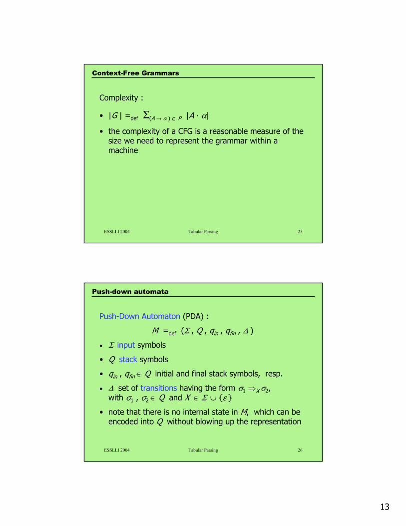
Context-Free Grammars
Complexity :
• |G | =def Σ(A → α ) ∈ P |A · α|
• the complexity of a CFG is a reasonable measure of the size we need to represent the grammar within a machine
ESSLLI 2004 Tabular Parsing 26
Push-Down Automaton (PDA) :
M =def (Σ , Q , qin , qfin , ∆ )
• Σ input symbols
• Q stack symbols
• qin , qfin ∈ Q initial and final stack symbols, resp.
• ∆ set of transitions having the form σ1 ⇒X σ2, with σ1 , σ2 ∈ Q and X ∈ Σ ∪ {ε }
• note that there is no internal state in M, which can be encoded into Q without blowing up the representation
Push-down automata
14
ESSLLI 2004 Tabular Parsing 27
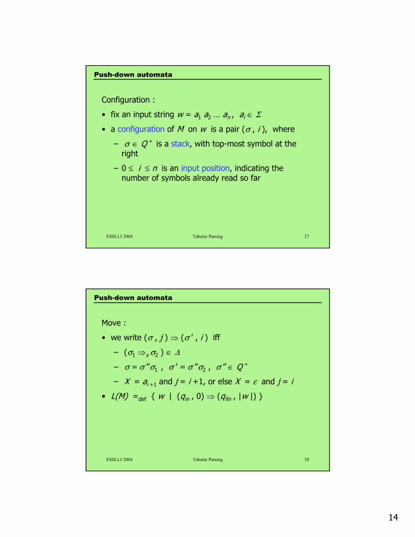
Configuration :
• fix an input string w = a1 a2 … an , ai ∈ Σ
• a configuration of M on w is a pair (σ , i ), where
– σ ∈ Q * is a stack, with top-most symbol at the right
– 0 ≤ i ≤ n is an input position, indicating the number of symbols already read so far
Push-down automata
ESSLLI 2004 Tabular Parsing 28
Move :
• we write (σ , j ) ⇒ (σ ’ , i ) iff
– (σ1 ⇒x σ2 ) ∈ ∆
– σ = σ ’’σ1 , σ ’ = σ ’’σ2 , σ ’’ ∈ Q *
– X = ai +1 and j = i +1, or else X = ε and j = i
• L(M) =def { w | (qin , 0) ⇒ (qfin , |w |) }
Push-down automata
15
ESSLLI 2004 Tabular Parsing 29
Push-down automata
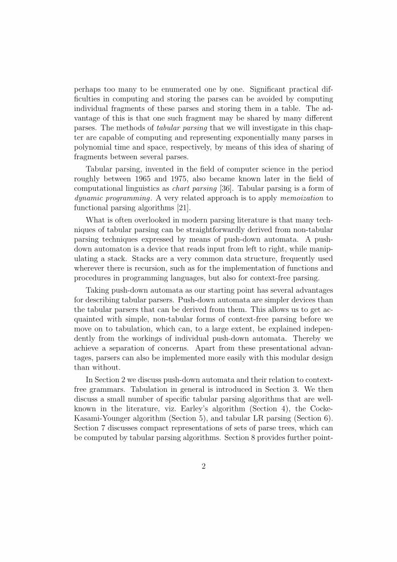
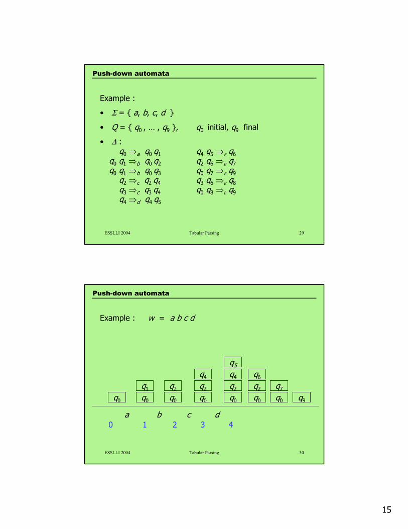
Example :
• Σ = { a, b, c, d }
• Q = { q0 , … , q9 }, q0 initial, q9 final
• ∆ : q0 ⇒a q0 q1 q4 q5 ⇒ε q6
q0 q1 ⇒b q0 q2 q2 q6 ⇒ε q7q0 q1 ⇒b q0 q3 q0 q7 ⇒ε q9
q2 ⇒c q2 q4 q3 q6 ⇒ε q8q3 ⇒c q3 q4 q0 q8 ⇒ε q9q4 ⇒d q4 q5
ESSLLI 2004 Tabular Parsing 30
Push-down automata
Example : w = a b c d
a cb d10
q0
q1
q0
q2
q0
q4
2
q2
q0
q4
q5
q2
q0
q2
q0
q6
q9
q7
q0
3 4
16
ESSLLI 2004 Tabular Parsing 31
Push-down automata
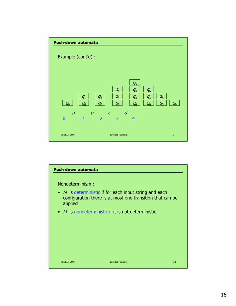
Example (cont’d) :
a cb d10
q0
q1
q0
q3
q0
q4
2
q3
q0
q4
q5
q3
q0
q3
q0
q6
q9
q8
q0
3 4
ESSLLI 2004 Tabular Parsing 32
Nondeterminism :
• M is deterministic if for each input string and each configuration there is at most one transition that can be applied
• M is nondeterministic if it is not deterministic
Push-down automata
17
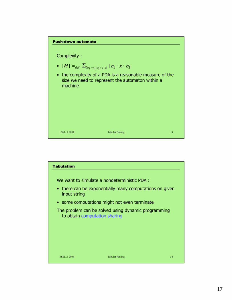
ESSLLI 2004 Tabular Parsing 33
Complexity :
• |M | =def Σ(σ1 ⇒x σ2) ∈ ∆ |σ1 · x · σ2|
• the complexity of a PDA is a reasonable measure of the size we need to represent the automaton within a machine
Push-down automata
ESSLLI 2004 Tabular Parsing 34
We want to simulate a nondeterministic PDA :
• there can be exponentially many computations on given input string
• some computations might not even terminate
The problem can be solved using dynamic programming to obtain computation sharing
Tabulation
18
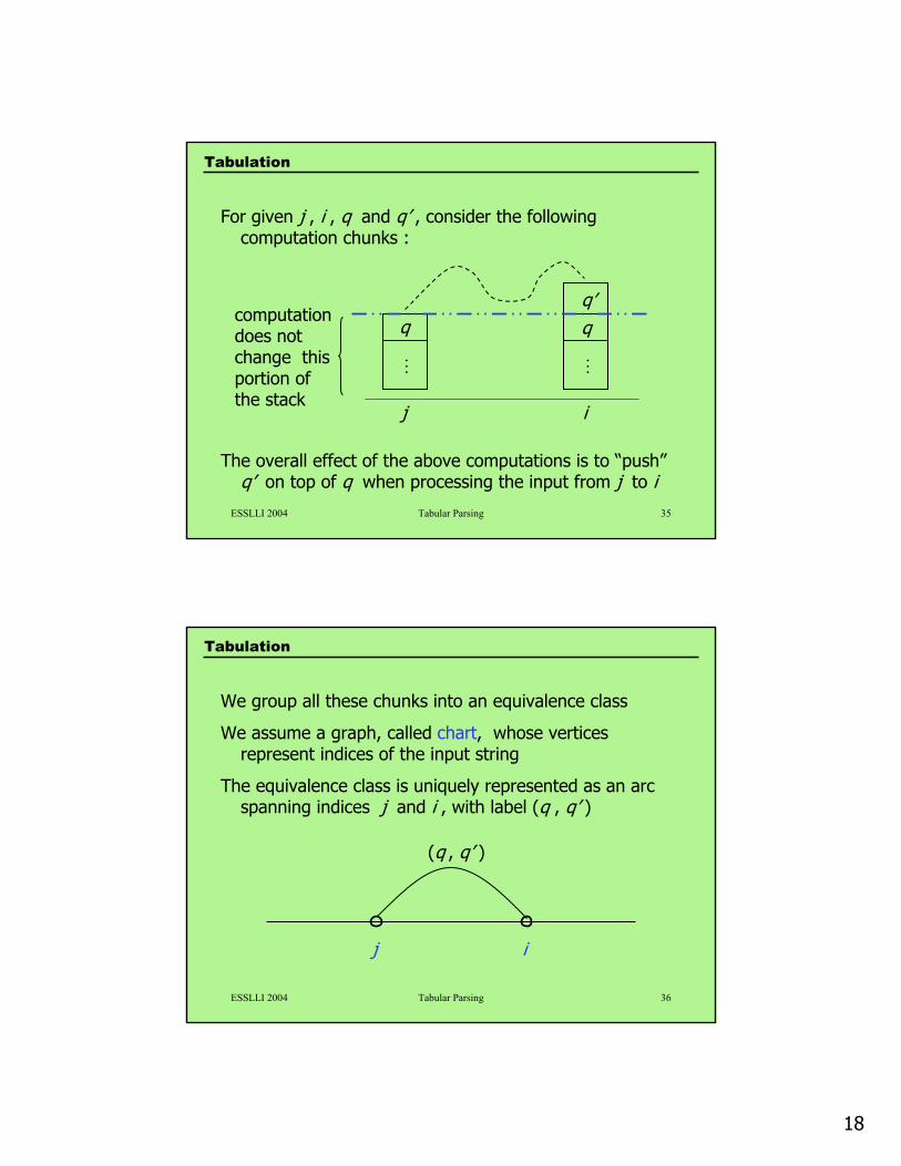
ESSLLI 2004 Tabular Parsing 35
For given j , i , q and q’ , consider the following computation chunks :
The overall effect of the above computations is to “push”q’ on top of q when processing the input from j to i
Tabulation
q
…
q’
…
q
j i
computation does not change this portion of the stack
ESSLLI 2004 Tabular Parsing 36
We group all these chunks into an equivalence class
We assume a graph, called chart, whose vertices represent indices of the input string
The equivalence class is uniquely represented as an arc spanning indices j and i , with label (q , q’ )
Tabulation
j i
(q , q’ )
19
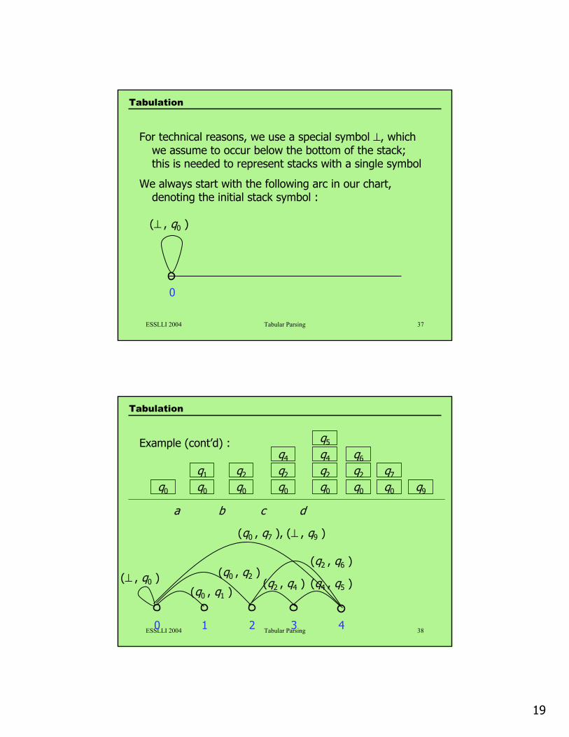
ESSLLI 2004 Tabular Parsing 37
For technical reasons, we use a special symbol ⊥, which we assume to occur below the bottom of the stack; this is needed to represent stacks with a single symbol
We always start with the following arc in our chart, denoting the initial stack symbol :
Tabulation
0
(⊥ , q0 )
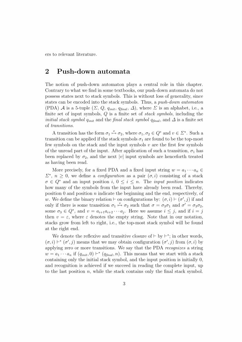
ESSLLI 2004 Tabular Parsing 3810 2 3 4
(q0 , q2 )
(q0 , q1 )(⊥ , q0 ) (q2 , q4 ) (q4 , q5 )
(q2 , q6 )
(q0 , q7 ), (⊥ , q9 )
a cb d
q0
q1
q0
q2
q0
q4
q2
q0
q4
q5
q2
q0
q2
q0
q6
q9
q7
q0
Example (cont’d) :
Tabulation
20
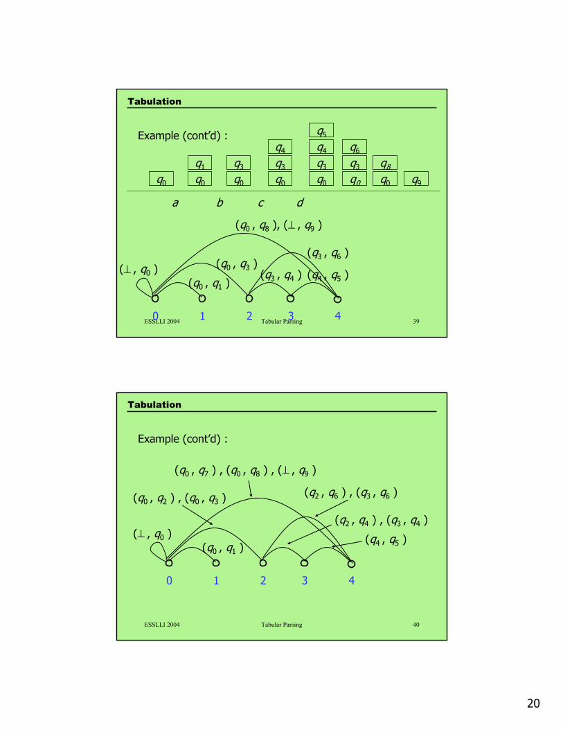
ESSLLI 2004 Tabular Parsing 3910 2 3 4
(q0 , q3 )
(q0 , q1 )(⊥ , q0 ) (q3 , q4 ) (q4 , q5 )
(q3 , q6 )
(q0 , q8 ), (⊥ , q9 )
a cb d
q0
q1
q0
q3
q0
q4
q3
q0
q4
q5
q3
q0
q3
q0
q6
q9
q8
q0
Example (cont’d) :
Tabulation
ESSLLI 2004 Tabular Parsing 40
10 2 3 4
(q0 , q1 )(⊥ , q0 ) (q4 , q5 )
(q2 , q6 ) , (q3 , q6 )
(q0 , q7 ) , (q0 , q8 ) , (⊥ , q9 )
(q0 , q2 ) , (q0 , q3 )
(q2 , q4 ) , (q3 , q4 )
Example (cont’d) :
Tabulation
21
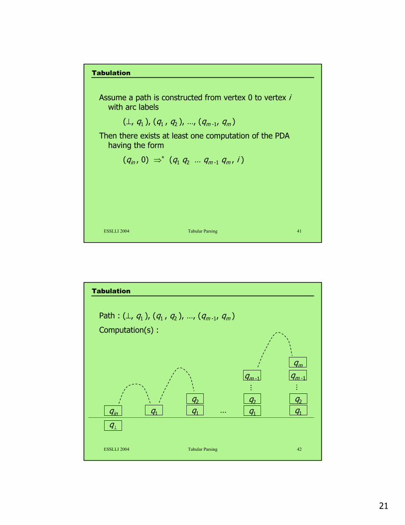
ESSLLI 2004 Tabular Parsing 41
Assume a path is constructed from vertex 0 to vertex iwith arc labels
(⊥, q1 ), (q1 , q2 ), …, (qm -1, qm )
Then there exists at least one computation of the PDA having the form
(qin , 0) ⇒* (q1 q2 … qm -1 qm , i )
Tabulation
ESSLLI 2004 Tabular Parsing 42
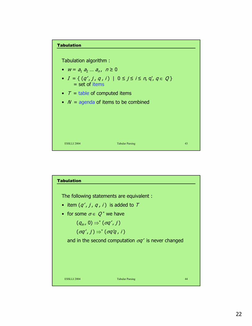
Path : (⊥, q1 ), (q1 , q2 ), …, (qm -1, qm )
Computation(s) :
Tabulation
qin q1
q2
q1
qm -1
q⊥
q2
q1
…
q2
q1
qm -1
qm
…
…
22
ESSLLI 2004 Tabular Parsing 43
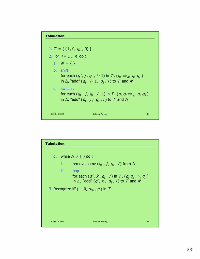
Tabulation algorithm :
• w = a1 a2 … an , n ≥ 0
• I = { (q’ , j , q , i ) | 0 ≤ j ≤ i ≤ n, q’, q ∈ Q }= set of items
• T = table of computed items
• N = agenda of items to be combined
Tabulation
ESSLLI 2004 Tabular Parsing 44
The following statements are equivalent :
• item (q’ , j , q , i ) is added to T
• for some σ ∈ Q * we have
(qin , 0) ⇒* (σq’ , j )
(σq’ , j ) ⇒* (σq’q , i )
and in the second computation σq’ is never changed
Tabulation
23
ESSLLI 2004 Tabular Parsing 45
Tabulation
1. T = { (⊥, 0, qin , 0) }
2. For i = 1 .. n do :
a. N = { }
b. shift :for each (q’ , j , q1 , i - 1) in T , (q1 ⇒ai q1 q2 ) in ∆, “add” (q1 , i - 1, q2 , i ) to T and N
c. switch :for each (q1 , j , q2 , i - 1) in T , (q1 q2 ⇒ai q1 q3 ) in ∆, “add” (q1 , j , q3 , i ) to T and N
ESSLLI 2004 Tabular Parsing 46
Tabulation
d. while N ≠ { } do :
i. remove some (q1 , j , q2 , i ) from N
ii. pop :for each (q’ , k , q1 , j ) in T , (q1 q2 ⇒ε q3 ) in ∆ , “add” (q’ , k , q3 , i ) to T and N
3. Recognize iff (⊥, 0, qfin , n ) in T
24
ESSLLI 2004 Tabular Parsing 47
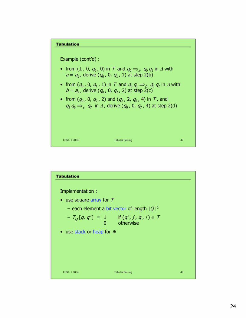
Example (cont’d) :
• from (⊥ , 0, q0 , 0) in T and q0 ⇒a q0 q1 in ∆ with a = a1 , derive (q0 , 0, q1 , 1) at step 2(b)
• from (q0 , 0, q1 , 1) in T and q0 q1 ⇒b q0 q2 in ∆ with b = a2 , derive (q0 , 0, q2 , 2) at step 2(c)
• from (q0 , 0, q2 , 2) and (q2 , 2, q6 , 4) in T , and q2 q6 ⇒ε q7 in ∆ , derive (q0 , 0, q7 , 4) at step 2(d)
Tabulation
ESSLLI 2004 Tabular Parsing 48
Implementation :
• use square array for T
– each element a bit vector of length |Q |2
– Ti,j [q, q’ ] = 1 if (q’ , j , q , i ) ∈ T0 otherwise
• use stack or heap for N
Tabulation
25
ESSLLI 2004 Tabular Parsing 49
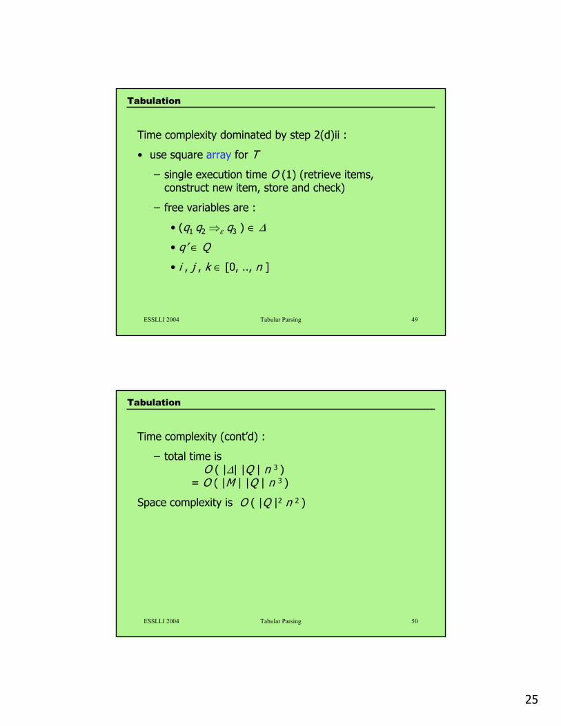
Time complexity dominated by step 2(d)ii :
• use square array for T
– single execution time O (1) (retrieve items, construct new item, store and check)
– free variables are :
• (q1 q2 ⇒ε q3 ) ∈ ∆
• q’ ∈ Q
• i , j , k ∈ [0, .., n ]
Tabulation
ESSLLI 2004 Tabular Parsing 50
Time complexity (cont’d) :
– total time is O ( |∆| |Q | n 3 )
= O ( |M | |Q | n 3 )
Space complexity is O ( |Q |2 n 2 )
Tabulation
26
ESSLLI 2004 Tabular Parsing 51
Tabulation
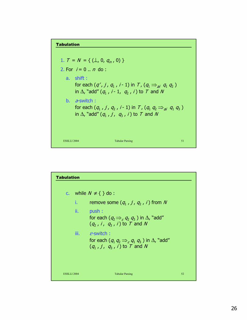
1. T = N = { (⊥, 0, qin , 0) }
2. For i = 0 .. n do :
a. shift :for each (q’ , j , q1 , i - 1) in T , (q1 ⇒ai q1 q2 ) in ∆, “add” (q1 , i - 1, q2 , i ) to T and N
b. a-switch :for each (q1 , j , q2 , i - 1) in T , (q1 q2 ⇒ai q1 q3 ) in ∆, “add” (q1 , j , q3 , i ) to T and N
ESSLLI 2004 Tabular Parsing 52
Tabulation
c. while N ≠ { } do :
i. remove some (q1 , j , q2 , i ) from N
ii. push :for each (q2 ⇒ε q2 q3 ) in ∆, “add”(q2 , i , q3 , i ) to T and N
iii. ε-switch :for each (q1 q2 ⇒ε q1 q3 ) in ∆, “add”(q1 , j , q3 , i ) to T and N
27
ESSLLI 2004 Tabular Parsing 53
Tabulation
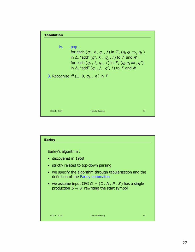
iv. pop :for each (q’ , k , q1 , j ) in T , (q1 q2 ⇒ε q3 ) in ∆, “add” (q’ , k , q3 , i ) to T and N ;for each (q2 , i , q3 , i ) in T , (q2 q3 ⇒ε q’ ) in ∆, “add” (q1 , j , q’ , i ) to T and N
3. Recognize iff (⊥, 0, qfin , n ) in T
ESSLLI 2004 Tabular Parsing 54
Earley’s algorithm :
• discovered in 1968
• strictly related to top-down parsing
• we specify the algorithm through tabularization and the definition of the Earley automaton
• we assume input CFG G = (Σ , N , P , S ) has a single production S → σ rewriting the start symbol
Earley
28
ESSLLI 2004 Tabular Parsing 55
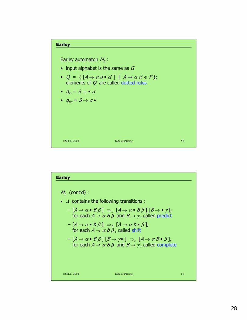
Earley automaton ME :
• input alphabet is the same as G
• Q = { [A → α a • α’ ] | A → α α’ ∈ P }; elements of Q are called dotted rules
• qin = S → • σ
• qfin = S → σ •
Earley
ESSLLI 2004 Tabular Parsing 56
ME (cont’d) :
• ∆ contains the following transitions :
– [A → α • B β ] ⇒ε [A → α • B β ] [B → • γ ], for each A → α B β and B → γ , called predict
– [A → α • b β ] ⇒b [A → α b • β ], for each A → α b β , called shift
– [A → α • B β ] [B → γ • ] ⇒ε [A → α B • β ], for each A → α B β and B → γ , called complete
Earley
29
ESSLLI 2004 Tabular Parsing 57
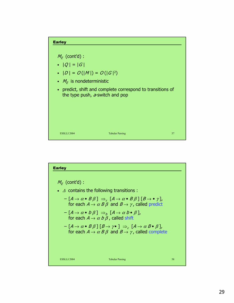
ME (cont’d) :
• |Q | = |G |
• |D | = O (|M |) = O (|G |2)
• ME is nondeterministic
• predict, shift and complete correspond to transitions of the type push, a-switch and pop
Earley
ESSLLI 2004 Tabular Parsing 58
ME (cont’d) :
• ∆ contains the following transitions :
– [A → α • B β ] ⇒ε [A → α • B β ] [B → • γ ], for each A → α B β and B → γ , called predict
– [A → α • b β ] ⇒b [A → α b • β ], for each A → α b β , called shift
– [A → α • B β ] [B → γ • ] ⇒ε [A → α B • β ], for each A → α B β and B → γ , called complete
Earley
30
ESSLLI 2004 Tabular Parsing 59
Earley
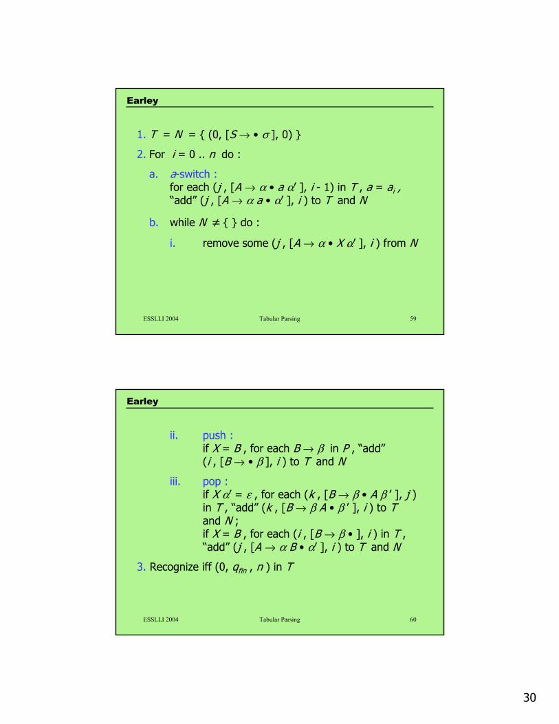
1. T = N = { (0, [S → • σ ], 0) }
2. For i = 0 .. n do :
a. a-switch :for each (j , [A → α • a α’ ], i - 1) in T , a = ai , “add” (j , [A → α a • α’ ], i ) to T and N
b. while N ≠ { } do :
i. remove some (j , [A → α • X α’ ], i ) from N
ESSLLI 2004 Tabular Parsing 60
ii. push :if X = B , for each B → β in P , “add”(i , [B → • β ], i ) to T and N
iii. pop :if X α’ = ε , for each (k , [B → β • A β ’ ], j ) in T , “add” (k , [B → β A • β ’ ], i ) to T and N ;if X = B , for each (i , [B → β • ], i ) in T ,“add” (j , [A → α B • α’ ], i ) to T and N
3. Recognize iff (0, qfin , n ) in T
Earley
31
ESSLLI 2004 Tabular Parsing 61
Cocke-Kasami-Younger
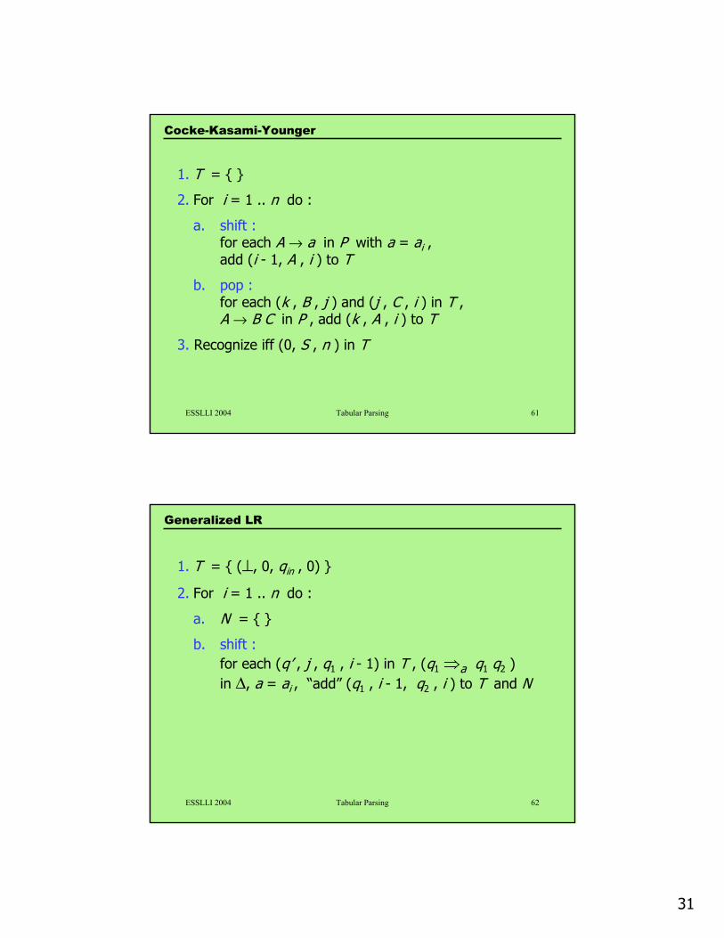
1. T = { }
2. For i = 1 .. n do :
a. shift :for each A → a in P with a = ai , add (i - 1, A , i ) to T
b. pop :for each (k , B , j ) and (j , C , i ) in T , A → B C in P , add (k , A , i ) to T
3. Recognize iff (0, S , n ) in T
ESSLLI 2004 Tabular Parsing 62
1. T = { (⊥, 0, qin , 0) }
2. For i = 1 .. n do :
a. N = { }
b. shift :for each (q’ , j , q1 , i - 1) in T , (q1 ⇒a q1 q2 ) in ∆, a = ai , “add” (q1 , i - 1, q2 , i ) to T and N
Generalized LR
32
ESSLLI 2004 Tabular Parsing 63
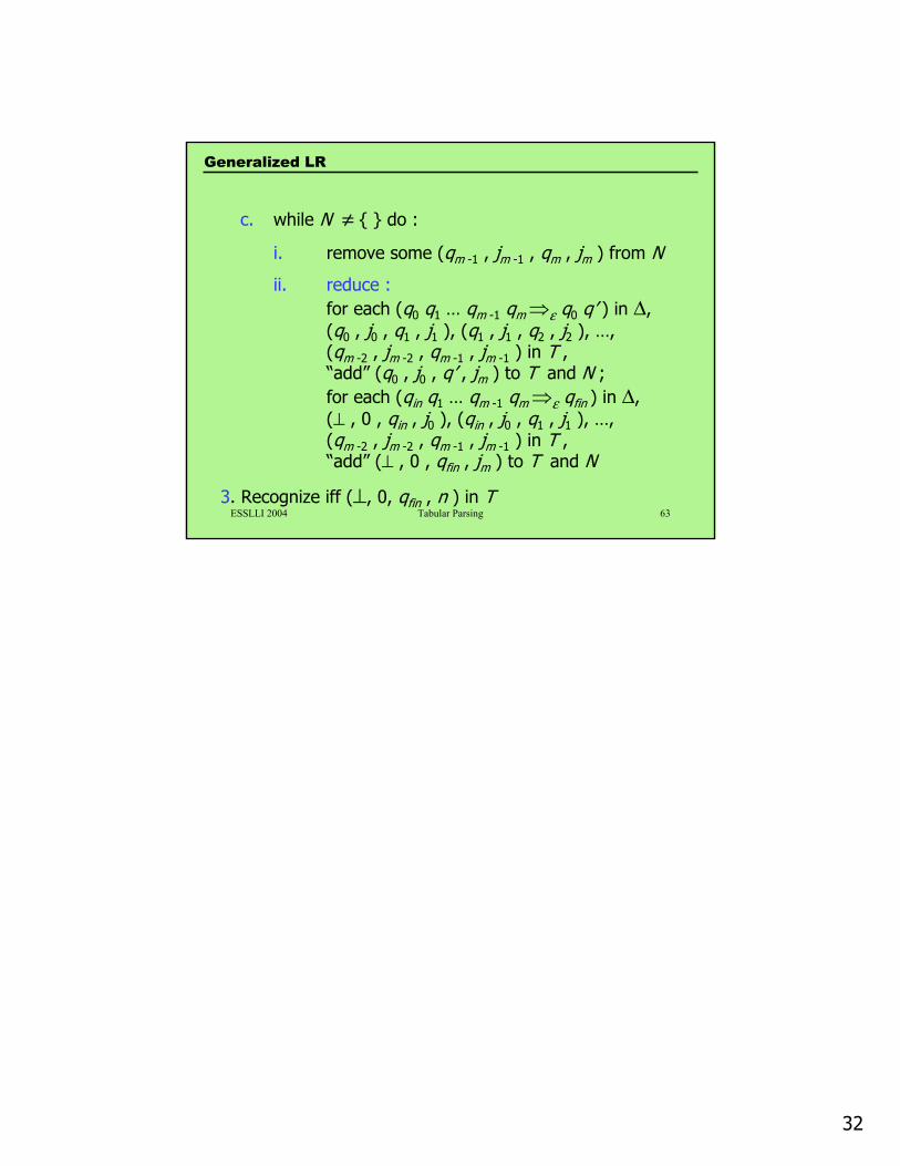
c. while N ≠ { } do :
i. remove some (qm -1 , jm -1 , qm , jm ) from N
ii. reduce :for each (q0 q1 … qm -1 qm⇒ε q0 q’ ) in ∆, (q0 , j0 , q1 , j1 ), (q1 , j1 , q2 , j2 ), …, (qm -2 , jm -2 , qm -1 , jm -1 ) in T , “add” (q0 , j0 , q’ , jm ) to T and N ;for each (qin q1 … qm -1 qm⇒ε qfin ) in ∆, (⊥ , 0 , qin , j0 ), (qin , j0 , q1 , j1 ), …, (qm -2 , jm -2 , qm -1 , jm -1 ) in T , “add” (⊥ , 0 , qfin , jm ) to T and N
3. Recognize iff (⊥, 0, qfin , n ) in T
Generalized LR