TabNet: A�entive Interpretable Tabular Learning

Sercan O. ArıkGoogle Cloud AI

soarik@google.com

Tomas P�sterGoogle Cloud AI

tp�ster@google.com

ABSTRACTWe propose a novel high-performance and interpretable canonicaldeep tabular data learning architecture, TabNet. TabNet uses se-quential a�ention to choose which features to reason from at eachdecision step, enabling interpretability and more e�cient learningas the learning capacity is used for the most salient features. Wedemonstrate that TabNet outperforms other neural network and de-cision tree variants on a wide range of non-performance-saturatedtabular datasets and yields interpretable feature a�ributions plusinsights into the global model behavior. Finally, for the �rst time toour knowledge, we demonstrate self-supervised learning for tabu-lar data, signi�cantly improving performance with unsupervisedrepresentation learning when unlabeled data is abundant.

KEYWORDSInterpretable deep learning, tabular data, a�ention, self-supervised.

1 INTRODUCTIONDeep neural networks (DNNs) have shown notable success withimages [21, 50], text [9, 34] and audio [1, 56]. For these data types,a major enabler of the progress is the availability of canonical DNNarchitectures that e�ciently encode the raw data into meaningfulrepresentations, resulting in high performance on new datasets andrelated tasks with minor e�ort. For example, in image understand-ing, variants of residual convolutional networks (e.g. ResNet [21])provide reasonably-well performance on new image datasets orslightly di�erent visual recognition problems (e.g. segmentation).

One data type that has yet to see such success with a canonicalDNN architecture is tabular data. Despite being the most commondata type in real-world AI1 [8], deep learning for tabular data re-mains under-explored, with variants of ensemble decision treesstill dominating most applications [28]. Why is this? First, be-cause tree-based approaches have certain bene�ts that make thempopular: (i) they are representionally e�cient (and thus o�en high-performing) for decision manifolds with approximately hyperplaneboundaries which are common in tabular data; and (ii) they arehighly interpretable in their basic form (e.g. by tracking decisionnodes) and there are e�ective post-hoc explainability methods fortheir ensemble form, e.g. [36] – this is an important concern inmany real-world applications (e.g. in �nancial services, wheretrust behind a high-risk action is crucial); (iii) they are fast to train.Second, because previously-proposed DNN architectures are notwell-suited for tabular data: conventional DNNs based on stackedconvolutional layers or multi-layer perceptrons (MLPs) are vastlyoverparametrized – the lack of appropriate inductive bias o�encauses them to fail to �nd optimal solutions for tabular decisionmanifolds [17].1As it corresponds to a combination of any unrelated categorical and numerical feature.

Why is deep learning worth exploring for tabular data? One obvi-ous motivation is that, similarly to other domains, one would expectperformance improvements from DNN-based architectures particu-larly for large datasets [22]. In addition, unlike tree learning whichdoes not use back-propagation into their inputs to guide e�cientlearning from the error signal, DNNs enable gradient descent-basedend-to-end learning for tabular data which can have a multitude ofbene�ts just like in the other domains it has already shown success:(i) it could e�ciently encode multiple data types like images alongwith tabular data; (ii) it would alleviate or eliminate the need forfeature engineering, which is currently a key aspect in tree-basedtabular data learning methods; (iii) it would enable learning fromstreaming data – tree learning needs global statistics to select splitpoints and straightforward modi�cations such as [4] typically yieldlower accuracy compared to learning from entire data – in contrast,DNNs show great potential for continual learning[44]; and per-haps most importantly (iv) end-to-end models allow representationlearning which enables many valuable new application scenariosincluding data-e�cient domain adaptation [17], generative mod-eling [46] and semi-supervised learning [11]. Clearly there aresigni�cant bene�ts in both tree-based and DNN-based methods. Isthere a way to design a method that has the most bene�cial aspectsof both?

In this paper, we propose a new canonical DNN architecture fortabular data, TabNet, that is designed to learn a ‘decision-tree-like’mapping in order to inherit the valuable bene�ts of tree-based meth-ods (interpretability and sparse feature selection), while providingthe key bene�ts of DNN-based methods (representation learningand end-to-end training). In particular, TabNet’s design considerstwo key needs: high performance and interpretability. As men-tioned, high performance alone is o�en not enough – a DNN needsto be interpretable to substitute tree-based methods. Overall, wemake the following contributions in the design of our method:

(1) Unlike tree-based methods, TabNet inputs raw tabular datawithout any feature preprocessing and is trained using gradientdescent-based optimization to learn �exible representations andenable �exible integration into end-to-end learning.

(2) TabNet uses sequential a�ention to choose which features to rea-son from at each decision step, enabling interpretability andbe�er learning as the learning capacity is used for the mostsalient features (see Fig. 1). �is feature selection is instance-wise, e.g. it can be di�erent for each input, and unlike otherinstance-wise feature selection methods like [6] or [61], Tab-Net employs a single deep learning architecture with end-to-endlearning.

(3) We show that the above design choices lead to two valuableproperties: (1) TabNet outperforms or is on par with other tabularlearning models on various datasets for classi�cation and regres-sion problems from di�erent domains; and (2) TabNet enables

arX

iv:1

908.

0744

2v4

[cs

.LG

] 1

4 Fe

b 20

20

Feature selection Input processing

Aggregate information

Feature selection Input processing

Predicted output (whether the income level >$50k)

Professional occupation related Investment related

Input features

Feedback from previous step

Feedback to next step

… …

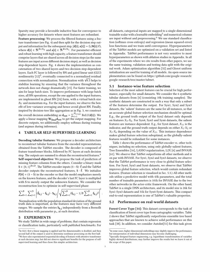
Figure 1: TabNet’s sparse feature selection exempli�ed for Adult Census Income prediction [14]. Sparse feature selectionenables interpretability and better learning as the capacity is used for the most salient features. TabNet employs multipledecision blocks that focus on processing a subset of input features for reasoning. Feature selection is based on feedback�owingfrom the preceding decision step. Two decision blocks shown as examples process features that are related to professionaloccupation and investments, respectively, in order to predict the income level.

Age Cap. gain Education Occupation Gender Relationship53 200000 ? Exec-managerial F Wife19 0 ? Farming-fishing M ?? 5000 Doctorate Prof-specialty M Husband

25 ? ? Handlers-cleaners F Wife59 300000 Bachelors ? ? Husband33 0 Bachelors ? F ?? 0 High-school Armed-Forces ? Husband

Age Cap. gain Education Occupation Gender RelationshipMasters

High-school Unmarried43

0 High-school FExec-managerial M

Adm-clerical Wife39 M

Income > $50kTrueFalseTrueFalseTrueTrueFalse

TabNet encoder

TabNet decoder Decision making

Age Cap. gain Education Occupation Gender Relationship60 200000 Bachelors Exec-managerial M Husband23 0 High-school Farming-fishing M Unmarried45 5000 Doctorate Prof-specialty M Husband23 0 High-school Handlers-cleaners F Wife56 300000 Bachelors Exec-managerial M Husband38 10000 Bachelors Prof-specialty F Wife23 0 High-school Armed-Forces M Husband

Unsupervised pre-training Supervised fine-tuning

TabNet encoder

Figure 2: Self-supervised tabular learning. Real-world tabular datasets have interdependent feature columns, e.g., the educa-tion level can be guessed from the occupation, or the gender can be guessed from the relationship. Unsupervised representa-tion learning by masked self-supervised learning results in an improved encoder model for the supervised learning task.

two kinds of interpretability: local interpretability that visualizesthe importance of input features and how they are combined,and global interpretability which quanti�es the contribution ofeach input feature to the trained model.

(4) Finally, we show that our canonical DNN design achieves sig-ni�cant performance improvements by using unsupervisedpre-training to predict masked features (see Fig. 2). Our workis the �rst demonstration of self-supervised learning for tabulardata.

2 RELATEDWORK

Feature selection: Feature selection in machine learning broadlyrefers to judiciously picking a subset of features based on their use-fulness for prediction. Commonly-used techniques such as forwardselection and LASSO regularization [20] a�ribute feature impor-tance based on the entire training data set, and are referred asglobal methods. Instance-wise feature selection refers to pickingfeatures individually for each input, studied in [6] by training anexplainer model to maximize the mutual information between theselected features and the response variable, and in [61] by using an

2

MaskM: [1, 0]

MaskM: [0, 1]

!"

!#

FCW: [$", - $", 0, 0]

b: [-a $", a $", -1, -1]

%

&

[!", !#]

[!"] [!#]!" > %!# < &

!" > %!# > &

!" < %!# > &

!" < %!# < &

$"!" − $"%−$"!" + $"%

−1−1

FCW: [0, 0, $# , - $# ]

b: [-1, -1, -d $#, d $# ]

−1−1

$#!# − $#&−$#!# + $#&

ReLU

+ Softmax

ReLU

Figure 3: Illustration of decision tree-like classi�cation using conventional DNN blocks (le�) and the corresponding decisionmanifold (right). Relevant features are selected by using multiplicative sparse masks on inputs. �e selected features arelinearly transformed, and a�er a bias addition (to represent boundaries) ReLUperforms region selection by zeroing the regionsthat are on the negative side of the boundary. Aggregation of multiple regions is based on addition. As C1 and C2 get larger,the decision boundary gets sharper due to the so�max.

actor-critic framework to mimic a baseline while optimizing thefeature selection. Unlike these, TabNet employs so� feature selectionwith controllable sparsity in end-to-end learning – a single modeljointly performs feature selection and output mapping, resulting insuperior performance with compact representations.Tree-based learning: Tree-based models are the most commonapproaches for tabular data learning. �e prominent strength oftree-based models is their e�cacy in picking global features with themost statistical information gain [18]. To improve the performanceof standard tree-based models by reducing the model variance, onecommon approach is ensembling. Among ensembling methods,random forests [23] use random subsets of data with randomlyselected features to grow many trees. XGBoost [7] and LightGBM[30] are the two recent ensemble decision tree approaches thatdominate most of the recent data science competitions. Our exper-imental results for various datasets show that tree-based modelscan be outperformed when the representation capacity is improvedwith deep learning while retaining their feature selecting property.

Integration of DNNs into decision trees: Representing deci-sion trees with canonical DNN building blocks as in [26] yieldsredundancy in representation and ine�cient learning. So� (neural)decision trees [33, 58] are proposed with di�erentiable decisionfunctions, instead of non-di�erentiable axis-aligned splits. How-ever, abandoning trees loses their automatic feature selection abilitywhich is important for tabular data. In [60], a so� binning functionis proposed to simulate decision trees in DNNs, which needs toenumerate all possible decisions and is ine�cient. [31] proposes aDNN architecture by explicitly leveraging expressive feature com-binations, however, learning is based on transferring knowledgefrom a gradient-boosted decision tree and limited performanceimprovements are observed. [53] proposes a DNN architectureby adaptively growing from primitive blocks while representationlearning into edges, routing functions and leaf nodes of a decisiontree. TabNet di�ers from these methods as it embeds the so� featureselection ability with controllable sparsity via sequential a�ention.Attentive table-to-text models: Table-to-text models extract tex-tual information from tabular data, for which recent works [3, 35]

propose a sequential mechanism for �eld-level a�ention. Unlikethese, we demonstrate the application of sequential a�ention forsupervised or self-supervised learning instead of mapping tabulardata to a di�erent data type.Self-supervised learning: Unsupervised representation learningis shown to bene�t the supervised learning task especially in smalldata regime [47]. Recent work for language [13] and image [55]data has shown signi�cant advances – speci�cally careful choice ofthe unsupervised learning objective (masked input prediction) anda�ention-based deep learning architecture is important.

3 TABNET FOR TABULAR LEARNINGDecision trees are successful for learning from real-world tabulardatasets. However, even conventional DNN building blocks can beused to implement decision tree-like output manifold – see Fig. 3)for an example. In such a design, individual feature selection is keyto obtain decision boundaries in hyperplane form. �is idea can begeneralized for a linear combination of features where constituentcoe�cients determine the proportion of each feature. TabNet isbased on such a tree-like functionality. We show that it outperformsdecision trees while reaping many of their bene�ts by careful de-sign which: (i) uses sparse instance-wise feature selection learnedbased on the training dataset; (ii) constructs a sequential multi-steparchitecture, where each decision step can contribute to a portion ofthe decision that is based on the selected features; (iii) improves thelearning capacity by non-linear processing of the selected features;and (iv) mimics an ensemble via higher dimensions and more steps.

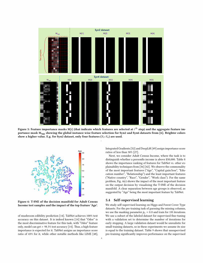
Fig. 4 shows the TabNet architecture for encoding tabular data.Tabular data are comprised of numerical and categorical features.We use the raw numerical features and consider mapping of categor-ical features with trainable embeddings2. We do not consider anyglobal normalization features, but merely apply batch normalization(BN). We pass the same D-dimensional features f ∈ <B×D to eachdecision step, where B is the batch size. TabNet’s encoding is basedon sequential multi-step processing with Nsteps decision steps. �eith step inputs the processed information from the (i − 1)th step2E.g., the three possible categories A, B and C for a particular feature can be learnedto be mapped to scalars 0.4, 0.1, and -0.2.

3

Features

Feature transformer

MaskAttentive transformer

+

Step 1

Feature transformer

Attentive transformer

BN

+FC BN

GLU

FC BN

GLU +FC BN

GLU

0.5

+FC BN

GLU

0.5 0.5

Shared across decision steps Decision step dependent

Split Split

FC BN

Sparsemax

+

Prior scales

+

…ReLU

MaskAttentive transformer

Split

ReLU

Step 2Output

+

Feature transformer

Feature transformer

Agg.

Featureattributes

+

Agg.

+ …

…

FC

(a) TabNet encoder architecture

Feature transformer

Step 1

+

Encoded representation

…

Reconstructed features

FC

Feature transformer

Step 2

FC

…

…(b) TabNet decoder architecture

Features

Feature transformer

Feature transformer

MaskAttentive transformer

+

x Nsteps

Feature transformer

Attentive transformer

Softmax

BN

+FC BN

GLU

FC BN

GLU +FC BN

GLU

0.5

+FC BN

GLU

0.5 0.5

Shared across decision steps Decision step dependent

Split Split

FC BN

Sparsemax

+

Prior scales

+

…

(c) Feature transformer

Features

Feature transformer

Feature transformer

MaskAttentive transformer

+

x Nsteps

Feature transformer

Attentive transformer

Softmax

BN

+FC BN

GLU

FC BN

GLU +FC BN

GLU

0.5

+FC BN

GLU

0.5 0.5

Shared across decision steps Decision step dependent

Split Split

FC BN

Sparsemax

+

Prior scales

+

…

(d) A�entive transformer

Figure 4: (a) TabNet encoder for classi�cation or regression, composed of a feature transformer, an attentive transformerand feature masking at each decision step. A split block divides the processed representation into two, to be used by theattentive transformer of the subsequent step as well as for constructing the overall output. At each decision step, the featureselection mask can provide interpretable information about the model’s functionality, and the masks can be aggregated toobtain global feature important attribution. (b) TabNet decoder, composed of a feature transformer block at each step. (c) Afeature transformer block example – 4-layer network is shown, where 2 of the blocks are shared across all decision steps and 2are decision step-dependent. Each layer is composed of a fully-connected (FC) layer, BN andGLUnonlinearity. (d) An attentivetransformer block example – a single layer mapping is modulated with a prior scale information which aggregates howmucheach feature has been used before the current decision step. Normalization of the coe�cients is done using sparsemax [37]for sparse selection of the most salient features at each decision step.

to decide which features to use and outputs the processed featurerepresentation to be aggregated into the overall decision. �e ideaof top-down a�ention in the sequential form is inspired by its ap-plications in processing visual and language data (e.g. in visualquestion answering [25]) and reinforcement learning [40] whilesearching for a small subset of relevant information in high dimen-sional input. Ablation studies in the Appendix focus on the impactof various design choices which are explained next. Guidelines onselection of the important hyperparameters are also provided inthe Appendix.Feature selection: We employ a learnable mask M[i] ∈ <B×D forso� selection of the salient features. �rough sparse selection of themost salient features, the learning capacity of a decision step is notwasted on irrelevant features, and thus the model becomes moreparameter e�cient. �e masking is in multiplicative form, M[i] · f .We use an a�entive transformer (see Fig. 4) to obtain the masksusing the processed features from the preceding step, a[i − 1]:

M[i] = sparsemax(P[i − 1] · hi (a[i − 1])). (1)

Sparsemax normalization [37] encourages sparsity by mappingthe Euclidean projection onto the probabilistic simplex, which is

observed to be superior in performance and aligned with the goalof sparse feature selection for most real-world datasets. Note thatEq. 1 ensures

∑Dj=1 M[i]b, j = 1. hi is a trainable function, shown in

Fig. 4 using a FC layer, followed by BN. P[i] is the prior scale term,denoting how much a particular feature has been used previously:

P[i] =∏i

j=1(γ −M[j]), (2)

where γ is a relaxation parameter – when γ = 1, a feature is en-forced to be used only at one decision step and as γ increases,more �exibility is provided to use a feature at multiple decisionsteps. P[0] is initialized as all ones, 1B×D , without any prior on themasked features. If some features are unused (as in self-supervisedlearning), corresponding P[0] entries are made 0 to help model’slearning. To further control the sparsity of the selected features,we propose sparsity regularization in the form of entropy [19]:

Lsparse =∑Nsteps

i=1

∑B

b=1

∑D

j=1

−Mb, j[i]Nsteps · B

log(Mb, j[i]+ϵ),

where ϵ is a small number for numerical stability. We add thesparsity regularization to the overall loss, with a coe�cient λsparse .

4

Sparsity may provide a favorable inductive bias for convergence tohigher accuracy for datasets where most features are redundant.Feature processing: We process the �ltered features using a fea-ture transformer (see Fig. 4) and then split for the decision step out-put and information for the subsequent step, [d[i], a[i]] = fi (M[i]·f),where d[i] ∈ <B×Nd and a[i] ∈ <B×Na . For parameter-e�cientand robust learning with high capacity, a feature transformer shouldcomprise layers that are shared across all decision steps (as the samefeatures are input across di�erent decision steps), as well as decisionstep-dependent layers. Fig. 4 shows the implementation as con-catenation of two shared layers and two decision step-dependentlayers. Each FC layer is followed by BN and gated linear unit (GLU)nonlinearity [12]3, eventually connected to a normalized residualconnection with normalization. Normalization with

√0.5 helps to

stabilize learning by ensuring that the variance throughout thenetwork does not change dramatically [15]. For faster training, weaim for large batch sizes. To improve performance with large batchsizes, all BN operations, except the one applied to the input features,are implemented in ghost BN [24] form, with a virtual batch sizeBV and momentummB . For the input features, we observe the ben-e�t of low-variance averaging and hence avoid ghost BN. Finally,inspired by decision-tree like aggregation as in Fig. 3, we constructthe overall decision embedding as dout =

∑Nstepsi=1 ReLU(d[i]). We

apply a linear mapping W�naldout to get the output mapping. Fordiscrete outputs, we additionally employ so�max during training(and argmax during inference).

4 TABULAR SELF-SUPERVISED LEARNING

Decoding tabular features: We propose a decoder architectureto reconstruct tabular features from the encoded representations,obtained from the TabNet encoder. �e decoder is composed offeature transformer blocks, followed by FC layers at each decisionstep. �e outputs are summed to obtain the reconstructed features.4Self-supervised objective: We propose the task of prediction ofmissing feature columns from the others. Consider a binary maskS ∈ {0, 1}B×D . �e TabNet encoder inputs (1−S) · f and the TabNetdecoder outputs the reconstructed features, S · f . We initializeP[0] = (1 − S) in the encoder so that the model emphasizes merelyon the known features, and the decoder’s last FC layer is multipliedwith S to merely output the unknown features. We consider thereconstruction loss to optimize in self-supervised phase:∑B

b=1

∑D

j=1

�����(fb, j − fb, j) · Sb, j/√∑B

b=1(fb, j − 1/B∑B

b=1 fb, j)2

�����2 .Normalization with the population standard deviation of the groundtruth data is important, as the features may have very di�erentranges. We sample the entries Sb, j independently from a Bernollidistribution with parameter ps , at each iteration.

5 EXPERIMENTSWe study TabNet in wide range of problems, that contain regressionor classi�cation tasks, particularly with published benchmarks. For3In GLU, �rst a linear mapping is applied and the dimensionality is doubled, and thensecond half of the output is used to determine nonlinear processing on the �rst half.4We have also experimented sequential decoding of features with a�entive transformerat each decision step, but did not observe signi�cant bene�ts for the purpose of self-supervised learning and thus chose this simpler architecture.

all datasets, categorical inputs are mapped to a single-dimensionaltrainable scalar with a learnable embedding5 and numerical columnsare input without and preprocessing.6 We use standard classi�ca-tion (so�max cross entropy) and regression (mean squared error)loss functions and we train until convergence. Hyperparametersof the TabNet models are optimized on a validation set and listedin Appendix. TabNet performance is not very sensitive to mosthyperparameters as shown with ablation studies in Appendix. In allof the experiments where we cite results from other papers, we usethe same training, validation and testing data split with the origi-nal work. Adam optimization algorithm [32] and Glorot uniforminitialization are used for training of all models. An open-source im-plementation can be found on h�ps://github.com/google-research/google-research/tree/master/tabnet.

5.1 Instance-wise feature selectionSelection of the most salient features can be crucial for high perfor-mance, especially for small datasets. We consider the 6 synthetictabular datasets from [6] (consisting 10k training samples). �esynthetic datasets are constructed in such a way that only a subsetof the features determine the output. For Syn1, Syn2 and Syn3datasets, the ‘salient’ features are the same for all instances, so thatan accurate global feature selection mechanism should be optimal.E.g., the ground truth output of the Syn2 dataset only dependson features X3-X6. For Syn4, Syn5 and Syn6 datasets, the salientfeatures are instance dependent. E.g., for Syn4 dataset, X11 is theindicator, and the ground truth output depends on either X1-X2 orX3-X6 depending on the value of X11. �is instance dependencemakes global feature selection suboptimal, as the globally-salientfeatures would be redundant for some instances.

Table 1 shows the performance of TabNet encoder vs. other tech-niques, including no selection, using only globally-salient features,Tree Ensembles [16], LASSO regularization, L2X [6] and INVASE[61]. We observe that TabNet outperforms all other methods and ison par with INVASE. For Syn1, Syn2 and Syn3 datasets, we observethat the TabNet performance is very close to global feature selec-tion. For Syn4, Syn5 and Syn6 datasets, we observe that TabNetimproves global feature selection, which would contain redundantfeatures. (Feature selection is visualized in Sec. 5.3.) All other meth-ods utilize a predictive model with 43k parameters, and the totalnumber of trainable parameters is 101k for INVASE due to the twoother networks in the actor-critic framework. On the other hand,TabNet is a single DNN architecture, and its model size is 26k forSyn1-Syn3 datasets and 31k for Syn4-Syn6 datasets. �is compactend-to-end representation is one of TabNet’s valuable properties.

5.2 Performance on real-world datasets

Forest Cover Type [14]: �is dataset corresponds to the task ofclassi�cation of forest cover type from cartographic variables. Table2 shows that TabNet signi�cantly outperforms ensemble tree basedapproaches that are known to achieve solid performance on thistask [38]. In addition, we consider AutoInt[51] for this task given

5In some cases, higher dimensional embeddings may slightly improve the performance,but interpretation of individual dimensions may become challenging.6Specially-designed feature engineering, e.g. logarithmic transformation of variableshighly-skewed distributions, may further improve the results but we leave it out ofthe scope of this paper.

5

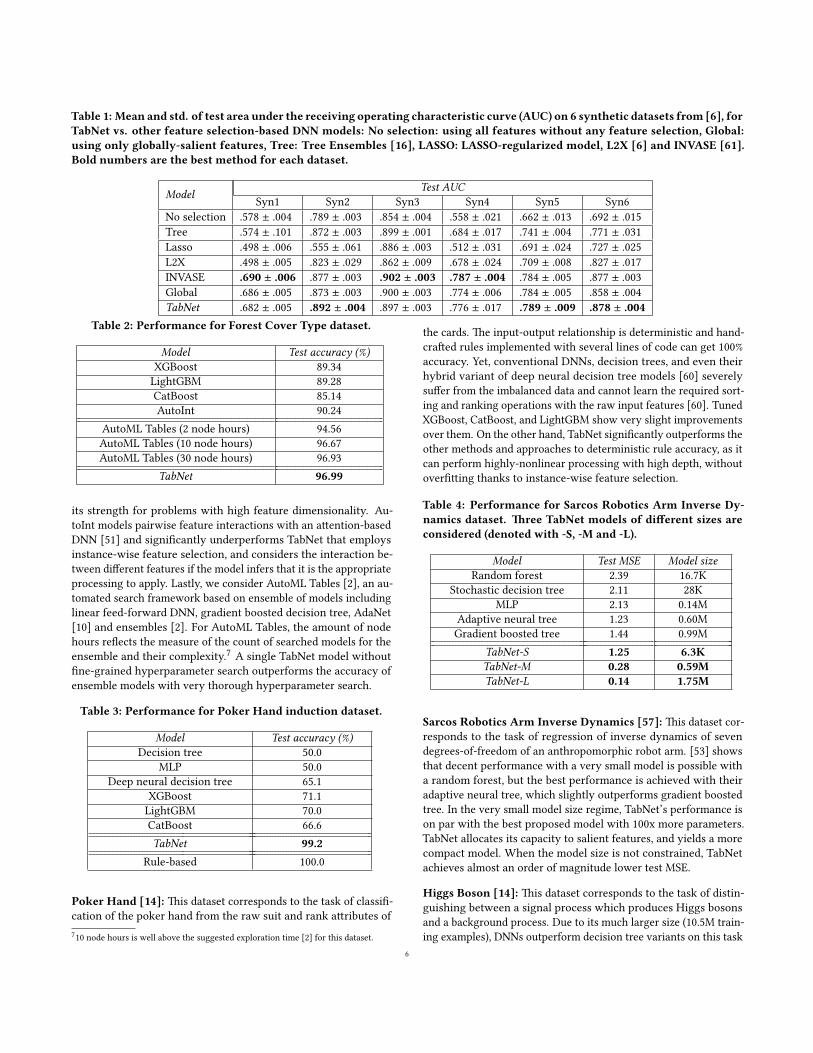
Table 1: Mean and std. of test area under the receiving operating characteristic curve (AUC) on 6 synthetic datasets from [6], forTabNet vs. other feature selection-based DNN models: No selection: using all features without any feature selection, Global:using only globally-salient features, Tree: Tree Ensembles [16], LASSO: LASSO-regularized model, L2X [6] and INVASE [61].Bold numbers are the best method for each dataset.

ModelTest AUC

Syn1 Syn2 Syn3 Syn4 Syn5 Syn6No selection .578 ± .004 .789 ± .003 .854 ± .004 .558 ± .021 .662 ± .013 .692 ± .015Tree .574 ± .101 .872 ± .003 .899 ± .001 .684 ± .017 .741 ± .004 .771 ± .031Lasso .498 ± .006 .555 ± .061 .886 ± .003 .512 ± .031 .691 ± .024 .727 ± .025L2X .498 ± .005 .823 ± .029 .862 ± .009 .678 ± .024 .709 ± .008 .827 ± .017INVASE .690 ± .006 .877 ± .003 .902 ± .003 .787 ± .004 .784 ± .005 .877 ± .003Global .686 ± .005 .873 ± .003 .900 ± .003 .774 ± .006 .784 ± .005 .858 ± .004TabNet .682 ± .005 .892 ± .004 .897 ± .003 .776 ± .017 .789 ± .009 .878 ± .004

Table 2: Performance for Forest Cover Type dataset.

Model Test accuracy (%)XGBoost 89.34

LightGBM 89.28CatBoost 85.14AutoInt 90.24

AutoML Tables (2 node hours) 94.56AutoML Tables (10 node hours) 96.67AutoML Tables (30 node hours) 96.93

TabNet 96.99

its strength for problems with high feature dimensionality. Au-toInt models pairwise feature interactions with an a�ention-basedDNN [51] and signi�cantly underperforms TabNet that employsinstance-wise feature selection, and considers the interaction be-tween di�erent features if the model infers that it is the appropriateprocessing to apply. Lastly, we consider AutoML Tables [2], an au-tomated search framework based on ensemble of models includinglinear feed-forward DNN, gradient boosted decision tree, AdaNet[10] and ensembles [2]. For AutoML Tables, the amount of nodehours re�ects the measure of the count of searched models for theensemble and their complexity.7 A single TabNet model without�ne-grained hyperparameter search outperforms the accuracy ofensemble models with very thorough hyperparameter search.

Table 3: Performance for Poker Hand induction dataset.

Model Test accuracy (%)Decision tree 50.0

MLP 50.0Deep neural decision tree 65.1

XGBoost 71.1LightGBM 70.0CatBoost 66.6TabNet 99.2

Rule-based 100.0

Poker Hand [14]: �is dataset corresponds to the task of classi�-cation of the poker hand from the raw suit and rank a�ributes of710 node hours is well above the suggested exploration time [2] for this dataset.

the cards. �e input-output relationship is deterministic and hand-cra�ed rules implemented with several lines of code can get 100%accuracy. Yet, conventional DNNs, decision trees, and even theirhybrid variant of deep neural decision tree models [60] severelysu�er from the imbalanced data and cannot learn the required sort-ing and ranking operations with the raw input features [60]. TunedXGBoost, CatBoost, and LightGBM show very slight improvementsover them. On the other hand, TabNet signi�cantly outperforms theother methods and approaches to deterministic rule accuracy, as itcan perform highly-nonlinear processing with high depth, withoutover��ing thanks to instance-wise feature selection.

Table 4: Performance for Sarcos Robotics Arm Inverse Dy-namics dataset. �ree TabNet models of di�erent sizes areconsidered (denoted with -S, -M and -L).

Model Test MSE Model sizeRandom forest 2.39 16.7K

Stochastic decision tree 2.11 28KMLP 2.13 0.14M

Adaptive neural tree 1.23 0.60MGradient boosted tree 1.44 0.99M

TabNet-S 1.25 6.3KTabNet-M 0.28 0.59MTabNet-L 0.14 1.75M

Sarcos Robotics Arm Inverse Dynamics [57]: �is dataset cor-responds to the task of regression of inverse dynamics of sevendegrees-of-freedom of an anthropomorphic robot arm. [53] showsthat decent performance with a very small model is possible witha random forest, but the best performance is achieved with theiradaptive neural tree, which slightly outperforms gradient boostedtree. In the very small model size regime, TabNet’s performance ison par with the best proposed model with 100x more parameters.TabNet allocates its capacity to salient features, and yields a morecompact model. When the model size is not constrained, TabNetachieves almost an order of magnitude lower test MSE.

Higgs Boson [14]: �is dataset corresponds to the task of distin-guishing between a signal process which produces Higgs bosonsand a background process. Due to its much larger size (10.5M train-ing examples), DNNs outperform decision tree variants on this task

6

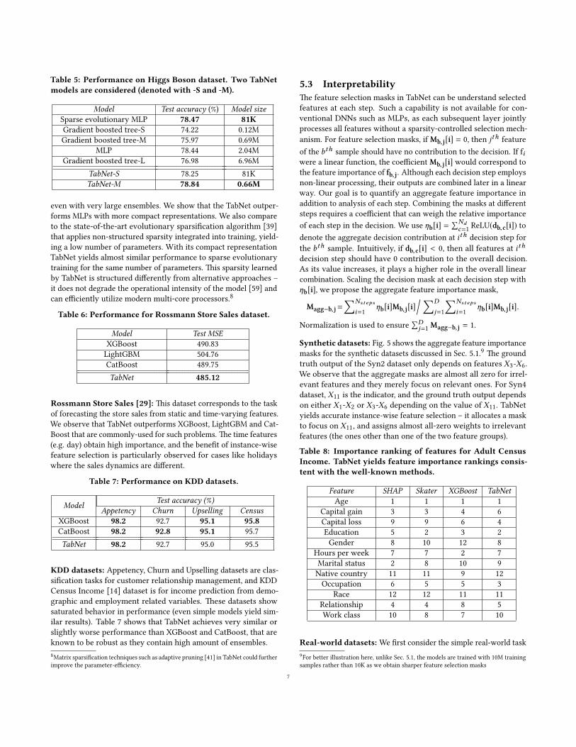
Table 5: Performance on Higgs Boson dataset. Two TabNetmodels are considered (denoted with -S and -M).

Model Test accuracy (%) Model sizeSparse evolutionary MLP 78.47 81KGradient boosted tree-S 74.22 0.12MGradient boosted tree-M 75.97 0.69M

MLP 78.44 2.04MGradient boosted tree-L 76.98 6.96M

TabNet-S 78.25 81KTabNet-M 78.84 0.66M

even with very large ensembles. We show that the TabNet outper-forms MLPs with more compact representations. We also compareto the state-of-the-art evolutionary sparsi�cation algorithm [39]that applies non-structured sparsity integrated into training, yield-ing a low number of parameters. With its compact representationTabNet yields almost similar performance to sparse evolutionarytraining for the same number of parameters. �is sparsity learnedby TabNet is structured di�erently from alternative approaches –it does not degrade the operational intensity of the model [59] andcan e�ciently utilize modern multi-core processors.8

Table 6: Performance for Rossmann Store Sales dataset.

Model Test MSEXGBoost 490.83

LightGBM 504.76CatBoost 489.75TabNet 485.12

Rossmann Store Sales [29]: �is dataset corresponds to the taskof forecasting the store sales from static and time-varying features.We observe that TabNet outperforms XGBoost, LightGBM and Cat-Boost that are commonly-used for such problems. �e time features(e.g. day) obtain high importance, and the bene�t of instance-wisefeature selection is particularly observed for cases like holidayswhere the sales dynamics are di�erent.

Table 7: Performance on KDD datasets.

ModelTest accuracy (%)

Appetency Churn Upselling CensusXGBoost 98.2 92.7 95.1 95.8CatBoost 98.2 92.8 95.1 95.7TabNet 98.2 92.7 95.0 95.5

KDD datasets: Appetency, Churn and Upselling datasets are clas-si�cation tasks for customer relationship management, and KDDCensus Income [14] dataset is for income prediction from demo-graphic and employment related variables. �ese datasets showsaturated behavior in performance (even simple models yield sim-ilar results). Table 7 shows that TabNet achieves very similar orslightly worse performance than XGBoost and CatBoost, that areknown to be robust as they contain high amount of ensembles.8Matrix sparsi�cation techniques such as adaptive pruning [41] in TabNet could furtherimprove the parameter-e�ciency.

5.3 Interpretability�e feature selection masks in TabNet can be understand selectedfeatures at each step. Such a capability is not available for con-ventional DNNs such as MLPs, as each subsequent layer jointlyprocesses all features without a sparsity-controlled selection mech-anism. For feature selection masks, if Mb, j[i] = 0, then jth featureof the bth sample should have no contribution to the decision. If fiwere a linear function, the coe�cient Mb, j[i] would correspond tothe feature importance of fb, j. Although each decision step employsnon-linear processing, their outputs are combined later in a linearway. Our goal is to quantify an aggregate feature importance inaddition to analysis of each step. Combining the masks at di�erentsteps requires a coe�cient that can weigh the relative importanceof each step in the decision. We use ηb[i] =

∑Ndc=1 ReLU(db,c[i]) to

denote the aggregate decision contribution at ith decision step forthe bth sample. Intuitively, if db,c[i] < 0, then all features at ithdecision step should have 0 contribution to the overall decision.As its value increases, it plays a higher role in the overall linearcombination. Scaling the decision mask at each decision step withηb[i], we propose the aggregate feature importance mask,

Magg−b, j=∑Nsteps

i=1 ηb[i]Mb, j[i]/ ∑D

j=1

∑Nsteps

i=1 ηb[i]Mb, j[i].

Normalization is used to ensure∑Dj=1 Magg−b, j = 1.

Synthetic datasets: Fig. 5 shows the aggregate feature importancemasks for the synthetic datasets discussed in Sec. 5.1.9 �e groundtruth output of the Syn2 dataset only depends on features X3-X6.We observe that the aggregate masks are almost all zero for irrel-evant features and they merely focus on relevant ones. For Syn4dataset, X11 is the indicator, and the ground truth output dependson either X1-X2 or X3-X6 depending on the value of X11. TabNetyields accurate instance-wise feature selection – it allocates a maskto focus on X11, and assigns almost all-zero weights to irrelevantfeatures (the ones other than one of the two feature groups).

Table 8: Importance ranking of features for Adult CensusIncome. TabNet yields feature importance rankings consis-tent with the well-known methods.

Feature SHAP Skater XGBoost TabNetAge 1 1 1 1

Capital gain 3 3 4 6Capital loss 9 9 6 4Education 5 2 3 2

Gender 8 10 12 8Hours per week 7 7 2 7Marital status 2 8 10 9

Native country 11 11 9 12Occupation 6 5 5 3

Race 12 12 11 11Relationship 4 4 8 5Work class 10 8 7 10

Real-world datasets: We �rst consider the simple real-world task9For be�er illustration here, unlike Sec. 5.1, the models are trained with 10M trainingsamples rather than 10K as we obtain sharper feature selection masks

7

/

M[1] M[2] M[3] M[4]Magg

Syn2 dataset

X11X1 X2 X3 X4 X5 X6 X7 X8 X9 X10

Test

sam

ples

M[1] M[2] M[3] M[4]Magg

Syn4 datasetM[5]

Figure 5: Feature importance masks M[i] (that indicate which features are selected at ith step) and the aggregate feature im-portance mask Magg showing the global instance-wise feature selection for Syn2 and Syn6 datasets from [6]. Brighter colorsshow a higher value. E.g. for Syn2 dataset, only four features (X3-X6) are used.

.

Figure 6: T-SNE of the decision manifold for Adult CensusIncome test samples and the impact of the top feature ‘Age’.

of mushroom edibility prediction [14]. TabNet achieves 100% testaccuracy on this dataset. It is indeed known [14] that “Odor” isthe most discriminative feature for this task, with “Odor” featureonly, model can get > 98.5% test accuracy [14]. �us, a high featureimportance is expected for it. TabNet assigns an importance scoreratio of 43% for it, while other notable methods like LIME [48],

Integrated Gradients [52] and DeepLi� [49] assign importance scoreratios of less than 30% [27].

Next, we consider Adult Census Income, where the task is todistinguish whether a person�s income is above $50,000. Table 8shows the importance ranking of features for TabNet vs. other ex-plainability techniques from [36] [42]. We observe the commonalityof the most important features (“Age”, “Capital gain/loss”, “Edu-cation number”, “Relationship”) and the least important features(“Native country”, “Race”, “Gender”, “Work class”). For the sameproblem, Fig. 6(c) shows the impact of the most important featureon the output decision by visualizing the T-SNE of the decisionmanifold. A clear separation between age groups is observed, assuggested by “Age” being the most important feature by TabNet.

5.4 Self-supervised learningWe study self-supervised learning on Higgs and Forest Cover Typedatasets. For the pre-training task of guessing the missing columns,we use the masking parameter ps = 0.8 and train for 1M iterations.We use a subset of the labeled dataset for supervised �ne-tuningwith a validation set to determine the number of iterations forearly stopping. A large validation dataset would be unrealistic forsmall training datasets, so in these experiments we assume its sizeis equal to the training dataset. Table 9 shows that unsupervisedpre-training signi�cantly improves performance on the supervised

8

Figure 7: Convergence with unsupervised pre-training ismuch faster, shown for Higgs dataset with 10k samples.

Table 9: Self-supervised tabular learning results. Mean andstd. of accuracy (over 15 runs) on Higgs with Tabnet-Mmodel, varying the size of the training dataset for super-vised �ne-tuning.

Training Test accuracy (%)dataset size Supervised With pre-training

1k 57.47 ± 1.78 61.37 ± 0.8810k 66.66 ± 0.88 68.06 ± 0.39100k 72.92 ± 0.21 73.19 ± 0.15

Table 10: Self-supervised tabular learning results. Mean andstd. of accuracy (over 15 runs) on Forest Cover Type, varyingthe size of the training dataset for supervised �ne-tuning.

Training Test accuracy (%)dataset size Supervised With pre-training

1k 65.91 ± 1.02 67.86 ± 0.6310k 78.85 ± 1.24 79.22 ± 0.78

classi�cation task, especially in the regime where the unlabeleddataset is much larger than the labeled dataset. As exempli�ed inFig. 7 the model convergence is much faster with unsupervised pre-training. Very fast convergence can be highly bene�cial particularlyin scenarios like continual learning and domain adaptation.

6 CONCLUSIONWe have proposed TabNet, a novel deep learning architecture fortabular learning. TabNet uses a sequential a�ention mechanismto choose a subset of semantically meaningful features to processat each decision step. Instance-wise feature selection enables ef-�cient learning as the model capacity is fully used for the mostsalient features, and also yields more interpretable decision makingvia visualization of selection masks. We demonstrate that TabNetoutperforms previous work across tabular datasets from di�erentdomains. Lastly, we demonstrate signi�cant bene�ts of unsuper-vised pre-training for fast adaptation and improved performance.

REFERENCES[1] Dario Amodei, Rishita Anubhai, Eric Ba�enberg, Carl Case, Jared Casper, et al.

2015. Deep Speech 2: End-to-End Speech Recognition in English and Mandarin.arXiv:1512.02595 (2015).

[2] AutoML. 2019. AutoML Tables – Google Cloud. h�ps://cloud.google.com/automl-tables/

[3] J. Bao, D. Tang, N. Duan, Z. Yan, M. Zhou, and T. Zhao. 2019. Text GenerationFrom Tables. IEEE Trans Audio, Speech, and Language Processing 27, 2 (Feb 2019),311–320.

[4] Yael Ben-Haim and Elad Tom-Tov. 2010. A Streaming Parallel Decision TreeAlgorithm. JMLR 11 (March 2010), 849–872.

[5] Catboost. 2019. Benchmarks. h�ps://github.com/catboost/benchmarks. Accessed:2019-11-10.

[6] Jianbo Chen, Le Song, Martin J. Wainwright, and Michael I. Jordan. 2018. Learn-ing to Explain: An Information-�eoretic Perspective on Model Interpretation.arXiv:1802.07814 (2018).

[7] Tianqi Chen and Carlos Guestrin. 2016. XGBoost: A Scalable Tree BoostingSystem. In KDD.

[8] Michael Chui, James Manyika, Mehdi Miremadi, Nicolaus Henke, Rita Chung,et al. 2018. Notes from the AI Frontier. McKinsey Global Institute (4 2018).

[9] Alexis Conneau, Holger Schwenk, Loıc Barrault, and Yann LeCun. 2016. VeryDeep Convolutional Networks for Natural Language Processing. arXiv:1606.01781(2016).

[10] Corinna Cortes, Xavi Gonzalvo, Vitaly Kuznetsov, Mehryar Mohri, and Sco�Yang. 2016. AdaNet: Adaptive Structural Learning of Arti�cial Neural Networks.arXiv:1607.01097 (2016).

[11] Zihang Dai, Zhilin Yang, Fan Yang, William W. Cohen, and Ruslan Salakhutdinov.2017. Good Semi-supervised Learning that Requires a Bad GAN. arxiv:1705.09783(2017).

[12] Yann N. Dauphin, Angela Fan, Michael Auli, and David Grangier. 2016. LanguageModeling with Gated Convolutional Networks. arXiv:1612.08083 (2016).

[13] Jacob Devlin, Ming-Wei Chang, Kenton Lee, and Kristina Toutanova. 2018. BERT:Pre-training of Deep Bidirectional Transformers for Language Understanding.arXiv:1810.04805 (2018).

[14] Dheeru Dua and Casey Gra�. 2017. UCI Machine Learning Repository. h�p://archive.ics.uci.edu/ml

[15] Jonas Gehring, Michael Auli, David Grangier, Denis Yarats, and Yann N. Dauphin.2017. Convolutional Sequence to Sequence Learning. arXiv:1705.03122 (2017).

[16] Pierre Geurts, Damien Ernst, and Louis Wehenkel. 2006. Extremely randomizedtrees. Machine Learning 63, 1 (01 Apr 2006), 3–42.

[17] Ian Goodfellow, Yoshua Bengio, and Aaron Courville. 2016. Deep Learning. MITPress.

[18] K. Grabczewski and N. Jankowski. 2005. Feature selection with decision treecriterion. In HIS.

[19] Yves Grandvalet and Yoshua Bengio. 2004. Semi-supervised Learning by EntropyMinimization. In NIPS.

[20] Isabelle Guyon and Andre Elissee�. 2003. An Introduction to Variable and FeatureSelection. JMLR 3 (March 2003), 1157–1182.

[21] Kaiming He, Xiangyu Zhang, Shaoqing Ren, and Jian Sun. 2015. Deep ResidualLearning for Image Recognition. arXiv:1512.03385 (2015).

[22] Joel Hestness, Sharan Narang, Newsha Ardalani, Gregory F. Diamos, HeewooJun, Hassan Kianinejad, Md. Mostofa Ali Patwary, Yang Yang, and Yanqi Zhou.2017. Deep Learning Scaling is Predictable, Empirically. arXiv:1712.00409 (2017).

[23] Tin Kam Ho. 1998. �e random subspace method for constructing decisionforests. PAMI 20, 8 (Aug 1998), 832–844.

[24] Elad Ho�er, Itay Hubara, and Daniel Soudry. 2017. Train longer, generalizebe�er: closing the generalization gap in large batch training of neural networks.arXiv:1705.08741 (2017).

[25] Drew A. Hudson and Christopher D. Manning. 2018. Compositional A�entionNetworks for Machine Reasoning. arXiv:1803.03067 (2018).

[26] K. D. Humbird, J. L. Peterson, and R. G. McClarren. 2018. Deep Neural NetworkInitialization With Decision Trees. IEEE Trans Neural Networks and LearningSystems (2018).

[27] Mark Ibrahim, Melissa Louie, Ceena Modarres, and John W. Paisley. 2019.Global Explanations of Neural Networks: Mapping the Landscape of Predic-tions. arxiv:1902.02384 (2019).

[28] Kaggle. 2019. Historical Data Science Trends on Kaggle. h�ps://www.kaggle.com/shivamb/data-science-trends-on-kaggle. Accessed: 2019-04-20.

[29] Kaggle. 2019. Rossmann Store Sales. h�ps://www.kaggle.com/c/rossmann-store-sales. Accessed: 2019-11-10.

[30] Guolin Ke, Qi Meng, �omas Finley, Taifeng Wang, Wei Chen, et al. 2017. Light-GBM: A Highly E�cient Gradient Boosting Decision Tree. In NIPS.

[31] Guolin Ke, Jia Zhang, Zhenhui Xu, Jiang Bian, and Tie-Yan Liu. 2019. TabNN: AUniversal Neural Network Solution for Tabular Data. h�ps://openreview.net/forum?id=r1eJssCqY7

[32] Diederik P. Kingma and Jimmy Ba. 2014. Adam: A Method for StochasticOptimization. In ICLR.

9

[33] P. Kontschieder, M. Fiterau, A. Criminisi, and S. R. Bul. 2015. Deep NeuralDecision Forests. In ICCV.

[34] Siwei Lai, Liheng Xu, Kang Liu, and Jun Zhao. 2015. Recurrent ConvolutionalNeural Networks for Text Classi�cation. In AAAI.

[35] Tianyu Liu, Kexiang Wang, Lei Sha, Baobao Chang, and Zhifang Sui. 2017.Table-to-text Generation by Structure-aware Seq2seq Learning. arXiv:1711.09724(2017).

[36] Sco� M. Lundberg, Gabriel G. Erion, and Su-In Lee. 2018. Consistent Individual-ized Feature A�ribution for Tree Ensembles. arXiv:1802.03888 (2018).

[37] Andre F. T. Martins and Ramon Fernandez Astudillo. 2016. From So�maxto Sparsemax: A Sparse Model of A�ention and Multi-Label Classi�cation.arXiv:1602.02068 (2016).

[38] Rory Mitchell, Andrey Adinets, �ejaswi Rao, and Eibe Frank. 2018. XGBoost:Scalable GPU Accelerated Learning. arXiv:1806.11248 (2018).

[39] Decebal Mocanu, Elena Mocanu, Peter Stone, Phuong Nguyen, MadeleineGibescu, and Antonio Lio�a. 2018. Scalable training of arti�cial neural net-works with adaptive sparse connectivity inspired by network science. NatureCommunications 9 (12 2018).

[40] Alex Mo�, Daniel Zoran, Mike Chrzanowski, Daan Wierstra, and Danilo J.Rezende. 2019. S3TA: A So�, Spatial, Sequential, Top-Down A�ention Model.h�ps://openreview.net/forum?id=B1gJOoRcYQ

[41] Sharan Narang, Gregory F. Diamos, Shubho Sengupta, and Erich Elsen. 2017.Exploring Sparsity in Recurrent Neural Networks. arXiv:1704.05119 (2017).

[42] Nbviewer. 2019. Notebook on Nbviewer. h�ps://nbviewer.jupyter.org/github/dipanjanS/data science for all/blob/master/tds model interpretation xai/Human-interpretableMachineLearning-DS.ipynb#

[43] N. C. Oza. 2005. Online bagging and boosting. In IEEE Trans Conference onSystems, Man and Cybernetics.

[44] German Ignacio Parisi, Ronald Kemker, Jose L. Part, Christopher Kanan, andStefan Wermter. 2018. Continual Lifelong Learning with Neural Networks: AReview. arXiv:1802.07569 (2018).

[45] Liudmila Prokhorenkova, Gleb Gusev, Aleksandr Vorobev, Anna Veronika Doro-gush, and Andrey Gulin. 2018. CatBoost: unbiased boosting with categoricalfeatures. In NIPS.

[46] Alec Radford, Luke Metz, and Soumith Chintala. 2015. Unsupervised Repre-sentation Learning with Deep Convolutional Generative Adversarial Networks.arXiv:1511.06434 (2015).

[47] Rajat Raina, Alexis Ba�le, Honglak Lee, Benjamin Packer, and Andrew Y. Ng.2007. Self-Taught Learning: Transfer Learning from Unlabeled Data. In ICML.

[48] Marco Ribeiro, Sameer Singh, and Carlos Guestrin. 2016. �Why Should I TrustYou?�: Explaining the Predictions of Any Classi�er. In KDD.

[49] Avanti Shrikumar, Peyton Greenside, and Anshul Kundaje. 2017. Learning Im-portant Features �rough Propagating Activation Di�erences. arXiv:1704.02685(2017).

[50] Karen Simonyan and Andrew Zisserman. 2014. Very Deep Convolutional Net-works for Large-Scale Image Recognition. arXiv:1409.1556 (2014).

[51] Weiping Song, Chence Shi, Zhiping Xiao, Zhijian Duan, Yewen Xu, Ming Zhang,and Jian Tang. 2018. AutoInt: Automatic Feature Interaction Learning via Self-A�entive Neural Networks. arxiv:1810.11921 (2018).

[52] Mukund Sundararajan, Ankur Taly, and Qiqi Yan. 2017. Axiomatic A�ributionfor Deep Networks. arXiv:1703.01365 (2017).

[53] Ryutaro Tanno, Kai Arulkumaran, Daniel C. Alexander, Antonio Criminisi, andAditya V. Nori. 2018. Adaptive Neural Trees. arXiv:1807.06699 (2018).

[54] Tensor�ow. 2019. Classifying Higgs boson processes in the HIGGS Data Set.h�ps://github.com/tensor�ow/models/tree/master/o�cial/boosted trees

[55] Trieu H. Trinh, Minh-�ang Luong, and �oc V. Le. 2019. Sel�e: Self-supervisedPretraining for Image Embedding. arXiv:1906.02940 (2019).

[56] Aaron van den Oord, Sander Dieleman, Heiga Zen, Karen Simonyan, OriolVinyals, et al. 2016. WaveNet: A Generative Model for Raw Audio.arXiv:1609.03499 (2016).

[57] Sethu Vijayakumar and Stefan Schaal. 2000. Locally Weighted Projection Re-gression: An O(n) Algorithm for Incremental Real Time Learning in High Di-mensional Space. In ICML.

[58] Suhang Wang, Charu Aggarwal, and Huan Liu. 2017. Using a random forest toinspire a neural network and improving on it. In SDM.

[59] Wei Wen, Chunpeng Wu, Yandan Wang, Yiran Chen, and Hai Li. 2016. LearningStructured Sparsity in Deep Neural Networks. arXiv:1608.03665 (2016).

[60] Yongxin Yang, Irene Garcia Morillo, and Timothy M. Hospedales. 2018. DeepNeural Decision Trees. arXiv:1806.06988 (2018).

[61] Jinsung Yoon, James Jordon, and Mihaela van der Schaar. 2019. INVASE: Instance-wise Variable Selection using Neural Networks. In ICLR.

APPENDIXA EXPERIMENT HYPERPARAMETERSFor all datasets, we use a pre-de�ned hyperparameter search space.Nd and Na are chosen from {8, 16, 24, 32, 64, 128}, Nsteps is cho-sen from {3, 4, 5, 6, 7, 8, 9, 10}, γ is chosen from {1.0, 1.2, 1.5, 2.0},λsparse is chosen from {0, 0.000001, 0.0001, 0.001, 0.01, 0.1}, B ischosen from {256, 512, 1024, 2048, 4096, 8192, 16384, 32768}, BV ischosen from {256, 512, 1024, 2048, 4096} and mB is chosen from{0.6, 0.7, 0.8, 0.9, 0.95, 0.98}. If the model size is not under the de-sired cuto�, we decrease the value to satisfy the size constraint. Forall the comparison models, we run a hyperparameter tuning withthe same number of search steps.Synthetic: All TabNet models use Nd=Na=16, B=3000, BV =100,mB=0.7. For Syn1 we use λsparse=0.02, Nsteps=4 and γ=2.0; forSyn2 and Syn3 we use λsparse=0.01, Nsteps=4 and γ=2.0; andfor Syn4, Syn5 and Syn6 we use λsparse=0.005, Nsteps=5 andγ=1.5. Feature transformers use two shared and two decision step-dependent FC layer, ghost BN and GLU blocks. All models useAdam with a learning rate of 0.02 (decayed 0.7 every 200 iterationswith an exponential decay) for 4k iterations. For visualizations inSec. 5.3, we also train TabNet models with datasets of size 10Msamples. For this case, we choose Nd = Na = 32, λsparse=0.001,B=10000, BV =100, mB=0.9. Adam is used with a learning rate of0.02 (decayed 0.9 every 2k iterations with an exponential decay)for 15k iterations. For Syn2 and Syn3, Nsteps=4 and γ=2. For Syn4and Syn6, Nsteps=5 and γ=1.5.Forest Cover Type: �e dataset partition details, and the hyperpa-rameters of XGBoost, LigthGBM, and CatBoost are from [38]. We re-optimize AutoInt hyperparameters. TabNet model uses Nd=Na=64,λsparse=0.0001, B=16384, BV =512,mB=0.7, Nsteps=5 and γ=1.5.Feature transformers use two shared and two decision step-dependentFC layer, ghost BN and GLU blocks. Adam is used with a learningrate of 0.02 (decayed 0.95 every 0.5k iterations with an exponen-tial decay) for 130k iterations. For unsupervised pre-training, thedecoder model uses Nd=Na=64, B=16384, BV =512, mB=0.7, andNsteps=10. For supervised �ne-tuning, we use the batch size B=BVas the training datasets are small.Poker Hands: We split 6k samples for validation from the train-ing dataset, and a�er optimization of the hyperparameters, weretrain with the entire training dataset. Decision tree, MLP anddeep neural decision tree models follow the same hyperparameterswith [60]. We tune the hyperparameters of XGBoost, LigthGBM,and CatBoost. TabNet uses Nd=Na=16, λsparse=0.000001, B=4096,BV =1024, mB = 0.95, Nsteps=4 and γ=1.5. Feature transformersuse two shared and two decision step-dependent FC layer, ghostBN and GLU blocks. Adam is used with a learning rate of 0.01(decayed 0.95 every 500 iterations with an exponential decay) for50k iterations.Sarcos: We split 4.5k samples for validation from the trainingdataset, and a�er optimization of the hyperparameters, we retrainwith the entire training dataset. All comparison models followthe hyperparameters from [53]. TabNet-S model uses Nd=Na=8,λsparse=0.0001, B=4096, BV =256, mB=0.9, Nsteps=3 and γ=1.2.Each feature transformer block uses one shared and two decisionstep-dependent FC layer, ghost BN and GLU blocks. Adam is usedwith a learning rate of 0.01 (decayed 0.95 every 8k iterations with

10

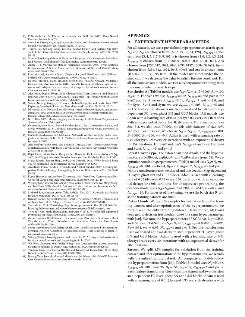
Table 11: Ablation studies for the TabNet encoder model for the forest cover type dataset.

Ablation casesTest accuracy% (di�erence)

Modelsize

Base (Nd = Na = 64, γ = 1.5, Nsteps = 5, λsparse = 0.0001, feature transformer block composed of two shared andtwo decision step-dependent layers, B = 16384) 96.99 470k

Decreasing capacity via number of units (with Nd = Na = 32) 94.99 (-2.00) 129kDecreasing capacity via number of decision steps (with Nsteps = 3) 96.22 (-0.77) 328kIncreasing capacity via number of decision steps (with Nsteps = 9) 95.48 (-1.51) 755k

Decreasing capacity via all-shared feature transformer blocks 96.74 (-0.25) 143kIncreasing capacity via decision step-dependent feature transformer blocks 96.76 (-0.23) 703k

Feature transformer block as a single shared layer 95.32 (-1.67) 35kFeature transformer block as a single shared layer, with ReLU instead of GLU 93.92 (-3.07) 27k

Feature transformer block as two shared layers 96.34 (-0.66) 71kFeature transformer block as two shared layers and 1 decision step-dependent layer 96.54 (-0.45) 271k

Feature transformer block as a single decision-step dependent layer 94.71 (-0.28) 105kFeature transformer block as a single decision-step dependent layer, with Nd=Na=128 96.24 (-0.75) 208k

Feature transformer block as a single decision-step dependent layer, with Nd=Na=128 and replacing GLU withReLU 95.67 (-1.32) 139k

Feature transformer block as a single decision-step dependent layer, with Nd=Na=256 and replacing GLU withReLU 96.41 (-0.58) 278k

Reducing the impact of prior scale (with γ = 3.0) 96.49 (-0.50) 470kIncreasing the impact of prior scale (with γ = 1.0) 96.67 (-0.32) 470k

No sparsity regularization (with λsparse = 0) 96.50 (-0.49) 470kHigh sparsity regularization (with λsparse = 0.01) 93.87 (-3.12) 470k

Small batch size (B = 4096) 96.42 (-0.57) 470k

an exponential decay) for 600k iterations. TabNet-M model usesNd=Na=64, λsparse=0.0001, B=4096, BV =128, mB=0.8, Nsteps=7and γ=1.5. Feature transformers use two shared and two decisionstep-dependent FC layer, ghost BN and GLU blocks. Adam is usedwith a learning rate of 0.01 (decayed 0.95 every 8k iterations withan exponential decay) for 600k iterations. �e TabNet-L model usesNd=Na=128, λsparse=0.0001, B=4096, BV =128,mB=0.8, Nsteps=5and γ=1.5. Feature transformers use two shared and two decisionstep-dependent FC layer, ghost BN and GLU blocks. Adam is usedwith a learning rate of 0.02 (decayed 0.9 every 8k iterations withan exponential decay) for 600k iterations.Higgs: We split 500k samples for validation from the trainingdataset, and a�er optimization of the hyperparameters, we re-train with the entire training dataset. MLP models are from [39].For gradient boosted trees [54], we tune the learning rate anddepth – the gradient boosted tree-S, -M, and -L models use 50,300 and 3000 trees respectively. TabNet-S model uses Nd=24,Na=26, λsparse=0.000001, B=16384, BV =512, mB=0.6, Nsteps=5and γ=1.5. Feature transformers use two shared and two deci-sion step-dependent FC layer, ghost BN and GLU blocks. Adam isused with a learning rate of 0.02 (decayed 0.9 every 20k iterationswith an exponential decay) for 870k iterations. TabNet-M modeluses Nd=96, Na=32, λsparse=0.000001, B=8192, BV =256, mB=0.9,Nsteps=8 and γ=2.0. Feature transformers use two shared and twodecision step-dependent FC layer, ghost BN and GLU blocks. Adamis used with a learning rate of 0.025 (decayed 0.9 every 10k itera-tions with an exponential decay) for 370k iterations. For unsuper-vised pre-training, the decoder model uses Nd=Na=128, B=8192,BV =256,mB=0.9, and Nsteps=20. For supervised �ne-tuning, we

use the batch size B=BV as the training datasets are small.Rossmann: We use the same preprocessing and data split with[5] – data from 2014 is used for training and validation, whereas2015 is used for testing. We split 100k samples for validationfrom the training dataset, and a�er optimization of the hyperpa-rameters, we retrain with the entire training dataset. �e perfor-mance of the comparison models are from [5]. TabNet model usesNd=Na=32, λsparse=0.001, B=4096, BV =512, mB=0.8, Nsteps=5and γ=1.2. Feature transformers use two shared and two decisionstep-dependent FC layer, ghost BN and GLU blocks. Adam is usedwith a learning rate of 0.002 (decayed 0.95 every 2000 iterationswith an exponential decay) for 15k iterations.KDD: For Appetency, Churn and Upselling datasets, we apply thesimilar preprocessing and split as [45]. �e performance of thecomparison models are from [45]. TabNet models use Nd=Na=32,λsparse=0.001, B=8192, BV =256, mB=0.9, Nsteps=7 and γ=1.2.Each feature transformer block uses two shared and two decisionstep-dependent FC layer, ghost BN and GLU blocks. Adam is usedwith a learning rate of 0.01 (decayed 0.9 every 1000 iterations withan exponential decay) for 10k iterations. For Census Income, thedataset and comparison model speci�cations follow [43]. TabNetmodel uses Nd=Na=48, λsparse=0.001, B=8192, BV =256, mB=0.9,Nsteps=5 and γ=1.5. Feature transformers use two shared andtwo decision step-dependent FC layer, ghost BN and GLU blocks.Adam is used with a learning rate of 0.02 (decayed 0.7 every 2000iterations with an exponential decay) for 4k iterations.Mushroomedibility: TabNet model usesNd=Na=8, λsparse=0.001,B=2048, BV =128,mB=0.9, Nsteps=3 and γ=1.5. Feature transform-ers use two shared and two decision step-dependent FC layer, ghost

11

BN and GLU blocks. Adam is used with a learning rate of 0.01(decayed 0.8 every 400 iterations with an exponential decay) for10k iterations.Adult Census Income: TabNet model usesNd=Na=16, λsparse =0.0001, B=4096, BV =128, mB=0.98, Nsteps=5 and γ=1.5. Featuretransformers use two shared and two decision step-dependent layer,ghost BN and GLU blocks. Adam is used with a learning rate of0.02 (decayed 0.4 every 2.5k iterations with an exponential decay)for 7.7k iterations. 85.7% test accuracy is achieved.

B ABLATION STUDIESTable 11 shows the impact of ablation cases. For all cases, thenumber of iterations is optimized on the validation set.

Obtaining high performance necessitates appropriately-adjustedmodel capacity based on the characteristics of the dataset. Decreas-ing the number of units Nd , Na or the number of decision stepsNsteps are e�cient ways of gradually decreasing the capacity with-out signi�cant degradation in performance. On the other hand,increasing these parameters beyond some value causes optimiza-tion issues and do not yield performance bene�ts. Replacing thefeature transformer block with a simpler alternative, such as a sin-gle shared layer, can still give strong performance while yieldinga very compact model architecture. �is shows the importance ofthe inductive bias introduced with feature selection and sequentiala�ention. To push the performance, increasing the depth of thefeature transformer is an e�ective approach. While increasing thedepth, parameter sharing between feature transformer blocks acrossdecision steps is an e�cient way to decrease model size withoutdegradation in performance. We indeed observe the bene�t of par-tial parameter sharing, compared to fully decision step-dependentblocks or fully shared blocks. We also observe the empirical bene�tof GLU, compared to conventional nonlinearities like ReLU.

�e strength of sparse feature selection depends on the twoparameters we introduce: γ and λsparse . We show that optimalchoice of these two is important for performance. A γ close to 1,or a high λsparse may yield too tight constraints on the strengthof sparsity and may hurt performance. On the other hand, there isstill the bene�t of a su�cient low γ and su�ciently high λsparse ,to aid learning of the model via a favorable inductive bias.

Lastly, given the �xed model architecture, we show the bene�t oflarge-batch training, enabled by ghost BN [24]. �e optimal batchsize for TabNet seems considerably higher than the conventionalbatch sizes used for other data types, such as images or speech.

C GUIDELINES FOR HYPERPARAMETERSWe consider datasets ranging from ∼10K to ∼10M samples, withvarying degrees of ��ing di�culty. TabNet obtains high perfor-mance on all with a few general principles on hyperparameters:

• For most datasets, Nsteps ∈ [3, 10] is optimal. Typically, whenthere are more information-bearing features, the optimal valueof Nsteps tends to be higher. On the other hand, increasingit beyond some value may adversely a�ect training dynamicsas some paths in the network becomes deeper and there aremore potentially-problematic ill-conditioned matrices. A veryhigh value of Nsteps may su�er from over��ing and yield poorgeneralization.

• Adjustment of Nd and Na is an e�cient way of obtaining atrade-o� between performance and complexity. Nd = Na is areasonable choice for most datasets. A very high value of Nd andNa may su�er from over��ing and yield poor generalization.

• An optimal choice of γ can have a major role on the performance.Typically a larger Nsteps value favors for a larger γ .• A large batch size is bene�cial – if the memory constraints permit,

as large as 1-10 % of the total training dataset size can helpperformance. �e virtual batch size is typically much smaller.

• Initially large learning rate is important, which should be gradu-ally decayed until convergence.

12