Table of Contents · Web viewThe solar radiation also has different components, Global Horizontal Irradiance (GHI), which is what Photovoltaic (PV) technology converts into power,

Forecasting and Characterising Grid Connected Solar Energy and Developing Synergies with WindProject results and lessons learnt

Lead organisation: University of New South WalesProject commencement date: 2011 Completion date: 2015Date published:Contact name: Merlinde KayTitle: DrEmail: [email protected] Phone: 02 9385 4031Website:

**Please use plain English – no jargon or unnecessary technical terms**

1

Table of ContentsTable of Contents..................................................................................................................................2

Executive Summary...............................................................................................................................3

Project Overview...................................................................................................................................4

Project summary............................................................................................................................4

Project scope.................................................................................................................................5

Outcomes......................................................................................................................................6

Transferability..............................................................................................................................21

Conclusion and next steps...........................................................................................................21

Lessons Learnt.....................................................................................................................................23

Lessons Learnt Report: Technical................................................................................................23

2

Executive Summary

Given the primary role played by non-renewable fossil fuel resources (e.g., coal and gas), the weather’s primary impact within the electricity industry is electrical demand, with a lesser impact seen in rainfall patterns and coal fired power station cooling requirements. But as greater proportions of renewable energies, such as solar and wind, are incorporated into the electricity mix, the weather and climate will begin to have an increasing impact on the supply-side also. New advances in meteorology and forecasting methods will be required that allow us to actively and effectively manage the impact of weather on both the demand, and renewable energy generation technologies, making them a more economically feasible option. The Project carried out data analysis and modelling to provide crucial information and decision support tools to assist in the deployment of solar technologies in a cost effective manner and facilitate synergistic operation of solar and wind technologies. This project explored the relationships between predictable weather patterns and the generation characteristics of key intermittent solar renewable technologies. Our results lead to metrics for site suitability for these technologies and, moreover, supported the development of a real-time forecasting scheme for solar renewable system output from forecasts of weather patterns and system performance data in line with National Electricity Market dispatch timeframes.

3

Project OverviewProject summary

This project aimed to contribute to the successful integration of high levels of intermittent solar renewable generation into the Australian electricity industry through advanced weather and climate forecasting tools.The innovative features of this project lie in the approach to the forecasting challenge. The forecasting challenge for Australia defies straightforward application of systems developed elsewhere. We have utilised innovative time series methods and mesoscale Numerical Weather Prediction (NWP) models. These forecasting techniques will allow management of the stochastic nature of these renewable technologies and allow appropriate mixes of flat plate PV, Concentrated Solar Technologies (PV and Solar Thermal) and wind to replace conventional power stations over time. Modelling of the synergies between solar and wind is a new feature to energy forecasting, as a combined solar and wind farm could provide great benefits to managing intermittent output due to weather systemsThe project covered three stages:Stage 1: Data Analysis – Characterising Variability

Analysis of the weather data at hourly intervals – insolation, cloud cover, temperature, wind speed and direction occurred for selected sites across Australia, looking at daily and seasonal variability to identify weather pattern cycles.

Identify weather patterns that would correlate to periods of low and high power production. Determine the effectiveness of weather prediction models to predict these weather events,

and their predictability over the short, medium and long-term at appropriate levels of geographical aggregation.

Stage 2: Develop Forecasting ToolsThere are many methods that can be used to develop a predictive model for solar system output from forecasts of weather patterns. A variety of approaches is needed as different forecasting tools have strengths and weaknesses at different time scales.

Approach 1, developing the predictive model utilising a prognostic meteorological and air prediction system that can incorporate data from a solar or wind farm and produce forecasts over a smaller geographical range.

Approach 2, for the sub-hourly timescale work is on developing structured models using classical time series methods for forecasting of solar radiation on various time scales.

Stage 3: Managing Large Penetrations of renewables Investigate output from potential individual solar energy systems and groups of systems, to

assess how they correlate with weather patterns and how this is influenced by geographic diversification.

Determine how to deal with distributed systems (rather than just central generating plants) taking into account how these systems will operate in response to weather events.

4

Compare output from solar energy systems with electricity loads on the distribution and transmission networks, and assess how solar output, as well as combined solar and wind output, affects these networks.

Project scopeGiven the heavy reliance in Australia on non-renewable fossil fuel resources (e.g., coal and gas), the weather’s primary impact on the electricity sector is on electrical demand. As greater proportions of renewable energies, such as solar and wind, are incorporated into the electricity mix, the weather and climate will begin to have an impact on the supply-side also. A key challenge for the large-scale adoption of solar power is the intermittent nature of the energy resource. The solar resource (solar radiation) is highly variable across daily and seasonal cycles, and influenced by factors such as absorption and scattering by clouds, water vapour, dust and pollutants that vary on time scales from minutes to years. Weather monitoring and forecasting has a key role in successfully managing the impact on both electricity demand and the output of renewable energy generation technologies, in order to make them economically viable options. Weather forecasting is the key challenge we faced in this work – the weather conditions determine the performance capacity of our intermittent renewable technologies. For example, changes to significant renewable generation due to cloud cover or strong winds as a cold front moves through can have a significant impact on power system efficiency and security. Better understanding of key aspects of the climatology, and better forecasts, can be used to guide investment and operational strategies. The forecasting techniques were for specific technologies; photovoltaics, both large scale solar farms and rooftop PV (distributed), and large scale solar thermal electricity. The operation of other electricity industry resources, particularly demand, can also be highly weather dependent; for example, heating and cooling loads. On a hot summer day, everyone turns their air-conditioners on at once, or cold winter days, heavy heating loads. This work aimed to solve the problem of the best way to forecast for solar technologies and the potential interactions between such solar technologies and wind over regional aggregations. There are growing Australian and international efforts to provide better forecasting and management tools for intermittent renewables. However, the Australian context defies straightforward application of systems developed elsewhere. Furthermore this project aims to extend current efforts through some novel techniques. For example, current prediction systems are generally lacking the small scale resolution that is required for location specific forecasts, and also understanding the relationship between the weather conditions and the specific technology that forecasts are required for. The effect of weather on each technology can vary on timescales from minutes to seasons, can be quite location specific and hence can effect where installations would be sited in terms of diversity of the region and the location of the grid. However, once installations are operational it is also necessary to predict and manage the impact of inevitable supply fluctuations. Of particular concern are periods of high solar output, which may present risks to power grids with high penetrations of solar technologies. These are areas that were yet to be examined and we addressed, to successfully manage solar technologies.We conducted a data analysis and modelling project to provide crucial information and decision support tools for increasing solar generation. We explored the relationships between predictable weather patterns and the generation characteristics of key intermittent solar renewable technologies. Our results lead to site suitability metrics for these technologies as well as supported the development of a real-time forecasting scheme for solar generation system output. We achieved

Report title | Page 5

this by applying new techniques and applications, as well as building upon wind forecasting tools previously developed by the research team. Different modelling techniques were utilised to predict future weather based on current observations, using a numerical forecast model and statistical techniques for a range of timescales. From this we predicted resource availability which is coincident with the weather. Techniques for deriving aggregated forecasts were developed. This will support an exploration of models for estimating the implications of different possible high renewable generation scenarios with regard to electricity industry operation.

OutcomesThis project was divided into three areas of research, site assessment, forecasting and managing large penetrations of renewables.Analysis of weather data to establish the ease of predictability of each weather pattern over different time-scales.The weather is essentially the fuel resource for renewable technologies. For solar technologies, this would be solar radiation. The solar radiation reaching the Earth’s surface can be affected by the time of year, cloud coverage, particles in the atmosphere and location. The solar radiation also has different components, Global Horizontal Irradiance (GHI), which is what Photovoltaic (PV) technology converts into power, and for concentrating solar technologies the Direct Normal Irradiance (DNI). Both are measured in Watts per metre squared (W/m2). The first stages of this project concentrated on weather data analysis. We are interested weather features that will affect the output from solar technologies such as frontal systems, and troughs, where we see changes in wind speed, wind direction and cloud cover. From this weather data analysis we were wanting to answer the following key questions:

What weather patterns are of greatest relevance to solar energy, along with frequency and duration;

What seasonal and yearly weather pattern cycles correlate to periods of low and high power production from solar technologies;

What is the coherence of weather-related power fluctuations over a large geographic region.Answering these questions assists in siting of future solar plants, and understanding operational constraints at specific times of year related to weather phenomena.We have analysed hourly satellite-derived solar irradiance data provided by the Australian Bureau of Meteorology (BoM) covering the period 1998 – 2010. This large data set enabled us to characterise the frequency and duration of protracted periods of low direct normal irradiance (DNI). By low DNI we refer to a threshold value of DNI where a concentrated solar plant would not be able to operate. For this work we took 400 W/m2 as that threshold value. These periods were then matched to Mean Sea Level Pressure (MSLP) maps to identify the weather phenomena/patterns that lead to these occurrences. An investigation was then carried out into the spatial relationship between the low periods of DNI, illustrating how geographic diversity of solar power stations, using concentrating solar power as an example, could help minimise the impact of these lows.


Figure 1. The longest period of consecutive days where the DNI is less than 400 W/m2 over the ten years of data analysed.

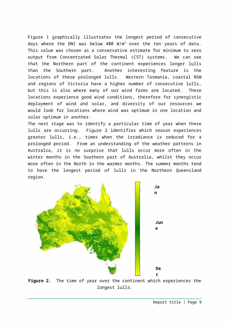
Figure 1 graphically illustrates the longest period of consecutive days where the DNI was below 400 W/m2 over the ten years of data. This value was chosen as a conservative estimate for minimum to zero output from Concentrated Solar Thermal (CST) systems. We can see that the Northern part of the continent experiences longer lulls than the Southern part. Another interesting feature is the locations of these prolonged lulls. Western Tasmania, coastal NSW and regions of Victoria have a higher number of consecutive lulls, but this is also where many of our wind farms are located. These locations experience good wind conditions, therefore for synergistic deployment of wind and solar, and diversity of our resources we would look for locations where wind was optimum in one location and solar optimum in another.The next stage was to identify a particular time of year when these lulls are occurring. Figure 2 identifies which season experiences greater lulls, i.e., times when the irradiance is reduced for a prolonged period. From an understanding of the weather patterns in Australia, it is no surprise that lulls occur more often in the winter months in the Southern part of Australia, whilst they occur more often in the North in the warmer months. The summer months tend to have the longest period of lulls in the Northern Queensland region.


Jan

June

Dec

Figure 2. The time of year over the continent which experiences the longest lulls.

The next stage identified a site from the North and South of the continent that could be potential sites due to their location. Roma was chosen in Queensland as it has previously been identified as a potential solar thermal site, and also has had solar monitoring as part of the Queensland Governments Solar Interactive Resource Map (http://www.brightthing.energy.qld.gov.au/bright-projects/queenslands-solar-atlas/). Roma also has a high voltage connection to the Queensland electricity grid and a natural gas-fired peaking power station, which could be useful during periods of lulls or low DNI. The Southern site chosen was Curnamona in South Australia as this site was identified as having the lowest number of consecutive lulls for the whole country.

Predict future weather based on current observations, using a numerical forecast model (for hourly and longer time frames) and statistical models (for sub-hourly)There are many methods that can be used to develop a predictive model for solar system output from forecasts of weather patterns. A variety of approaches is needed as different forecasting tools have strengths and weaknesses at different time scales. Different modelling techniques were utilised to predict future weather based on current observations, using a numerical forecast model and statistical techniques for a range of timescales. The two approaches were:

Approach 1, developing the predictive model utilising Numerical Weather Prediction (NWP) models; a prognostic meteorological and air prediction system (TAPM) that can incorporate data from a solar or wind farm and produce forecasts over a smaller geographical range, and utilising the Weather Research and Forecasting Model (WRF).

Approach 2, for the sub-hourly timescale work structured models were developed using classical time series methods for forecasting of solar radiation on various time scales.

Approach 1 – Numerical model forecasting


The first stage of this work was investigating the accuracy of The Air Pollution Model (TAPM) in estimating Global Horizontal Irradiance (GHI) at selected sites (see Table 1).

Table 1. Locations of the project sitesSite name Latitude (degree) Longitude (degree) StatesCloncurry -20.707 140.505 QLDRoma -26.535 148.779 QLDMoree -29.494 147.198 NSWBroken Hill -32.001 141.469 NSWBungendore -35.256 149.440 NSW Mildura -34.236 142.087 VICSwan Hill -35.377 143.542 VICCurnamona -31.475 139.642 SA

These sites were chosen as they have been identified as potential solar sites. The model uses standard meteorological fields but with no real-time cloud/aerosol information. In order to assess the model, TAPM-estimated GHI is compared to satellite-derived GHI at selected sites in Eastern Australia. The satellite derived data from the Bureau of Meteorology (BoM) covers a 5km grid spanning all of Australia. The satellite data used in this study was compared to ground-based observations at the Australian Bureau of Meteorology stations. The satellite data was corrected via a regression technique and adjusted accordingly.The model can be run at various spatial resolutions, by spatial resolution we mean the distance between grid points which we can get forecasts for, covering large to smaller areas. The sensitivity to spatial resolution was examined to determine the performance of TAPM for the chosen horizontal resolutions (45, 15, 5, 1.5, 0.5 km). We were wanting to determine the optimum resolution at which the model performs the best. The metrics chosen for this task are the annual RMSE (Root Mean Square Error) and MBE (Mean Bias Error). Using the RMSE and MBE provide information on the short-term and long-term performance of a model. However, one should keep in mind that a few large errors can increase the RMSE significantly, and in the case of MBE, over-estimation and under-estimation of observations can cancel out each other.


Figure 3. The RMSE and MBE of TAPM for different resolutions of the model at different hours (9am-3pm) in 2005; (a) RMSE at Mildura, (b) MBE at Mildura, (c) RMSE at Cloncurry and (d) MBE at

Cloncurry; error statistics measured with respect to corrected-satellite GHI.

The results revealed that a resolution of 45 km had the lowest Root Mean Square Error (RMSE). Figure 3a) and c) show the RMSE for Mildura and Cloncurry respectively, and Figs. 3b) and d) the MBE for the two sites. Most of the chosen sites display a similar trend in terms of RMSE and MBE to Mildura, with the highest RMSE at noon. In terms of looking at all project sites Cloncurry and Curnamona differ in this trend with the RMSE higher in the morning and decreasing towards afternoon. This means that variations on scales less than 45 km cannot be captured by the model properly. We also found that during cloudy conditions, the RMSE could increase by around 300 % compared to clear-sky conditions for both lower and higher resolutions. Therefore, most of the large errors that occur during cloudy conditions are associated with the misrepresentation of clouds in the model, in particular during deep low-pressure systems, passage of cold fronts, Easterly troughs, cloud bands, and in some conditions even during high pressure systems. We therefore applied a correction to the 45 km spatial resolution modelled GHI for clear-sky errors to improve the accuracy of the model. The same regression technique that we applied to correct the satellite data is applied here and resulted in a reduction of the RMSE, Mean Absolute Error (MAE) and Mean Bias Error (MBE) on average by a of maximum 16 %, 26 % and 84 % respectively.


The other forecasting model we were interested in verifying was the Weather Research and Forecasting (WRF) model. We were particularly interested in its ability to forecast extreme weather events and to this end chose a storm event that occurred in 2005, focusing on the impact of the storm around Mildura. Different physics parameterisation schemes were run to determine the optimal configuration to run the model. The absolute errors associated with the optimum model run are shown in Figure 4 (a) and (b) for GHI and DNI respectively for 00 UTC of February 3, 2005. It can be seen that the largest errors occurred in the region affected by the storm and the cloudy conditions associated with it.

Figure 4. WRF absolute errors associated with (a) GHI and (b) DNI for the period of 00 UTC of February 2nd till 00 UTC of February 3rd, 2005

WRF underestimated the spatial extent of clouds over Victoria, New South Wales and South Australia. Comparisons of the WRF-simulated solar irradiance with satellite- derived data showed that the performance of WRF was not impacted significantly by the choice of physics parameterisations during cloudy conditions. An increase in spatial resolution did not improve the performance of the model and increased the RMSE by 5% and 7% for GHI and DNI respectively during clear sky and by a maximum of 13% (GHI) and 7% (DNI) during cloudy conditions. WRF simulated GHI more accurately than DNI. The performance of the model generally did not improve with higher resolutions.In comparing the performance of WRF to TAPM, TAPM was run at 4 different resolutions, also finding that accuracy, if looking at RMSE alone, did not really improve with a finer resolution. The coarser resolution often was the most accurate, even though differences between the coarser and fine resolution only differed by 5 – 15 Wm-2 for all sky conditions, for both TAPM and WRF respectively. Greater differences were seen in MBE for WRF than TAPM.Overall both models had their advantages when forecasting solar radiation. WRF however has the added benefit of being able to forecast DNI, which is important when investigating both PV and Concentrated Solar Technologies (CST).


Approach 2 – Short term statistical forecastingA major outcome in the project as performed at University of South Australia has been the development of the Coupled Auto Regressive and Dynamical System (CARDS) short term forecasting system. It has been extensively tested on data from Australia, as well as from French offshore island locations, Guadeloupe and Reunion Island. This testing has been on time scales of ten minutes to one hour.The key to the success of this tool is the comprehensive determination of seasonal attributes of global solar radiation. While many researchers use co-called clear sky models to multiplicatively de-season the data, our approach was to let the measured data tell us about what specific seasonal attributes there are present. In other words, we let the data tell us about the underlying physics inherent in solar radiation.There are essentially two methods of dealing with the seasonalities inherent in climate variables. One can deal with it in a multiplicative or additive modelling framework. There are two versions of the multiplicative approach with respect to solar radiation, calculating the clearness index, and estimating the clear sky index. Additive de-seasoning is enacted through subtracting a mean function from the solar radiation, that function formed usually through the addition of terms involving a basis of the function space. An appropriate way to perform this operation is through the use of a Fourier set of basis functions.In a statistical sense, if sufficient years are used for the parameter estimation, the expected value for each time period is given. Also, there are simple formulae for calculating the amount of variance in the data explained at each chosen frequency. In a physical sense, the Fourier series model gives the climate for the location. In a very practical sense, the whole process is data driven.

An example of the Fourier series model for a few days of a solar radiation series is given in Figure 5.

Figure 5: An example Fourier fitSubsequent to the additive removal of the seasonality, the residual series is modelled via principally an autoregressive series, using the Box-Jenkins methodology. Then the final forecast model is a combination of the Fourier Series plus the AR(p) model. Note that the same method works for series


of solar radiation in any climate that we have studied. Figures 6 and 7 show the performance on a clear and cloudy day respectively.

Figure 6: The forecast model on a clear day

Figure 7: The forecast model on a cloudy day

When producing forecasts from models such as TAPM, only the GHI is forecast. Often one also needs DNI, especially if interested in CST. The group at the University of South Australia have developed a model for decomposing GHI into its direct and diffuse components. First, a logistic model for direct normal solar radiation using multiple location data was constructed. Afterwards, the Boland-Ridley-Lauret (BRL) model was used to obtain hourly diffuse radiation and from that direct normal solar radiation. Figures 8 and 9 show the BRL model fit for diffuse radiation and direct normal (DNI) respectively.


Figure 8: The BRL global to diffuse radiation model

Figure 9: The BRL global to DNI model

Considering all locations and error analyses, the results show that the BRL model is well equipped to not just estimate the diffuse solar irradiance from the global solar, but also to go from there to estimate the direct normal irradiance.

Determining optimal orientations and placements of solar energy systems to match electricity loads and to complement anticipated wind output taking into account the supply-demand balance.We have approached this work looking at two different aspects of placement of solar energy systems; centralised and distributed PV. Centralised refers to large scale generation plants connected to the electricity network, distributed refers to systems such as rooftop PV.


Centralised: Select PV locations were chosen - Adelaide, Brisbane, Canberra, Melbourne, Sydney, Cobar (NSW), Dalby (QLD), Long Reach (QLD), Mildura (Vic), White Cliffs (NSW), Whyalla (SA) and Woomera (SA) (see Figure 10, which displays the map of selected locations).

Figure 10. Selected PV locations spread across the Australian National Electricity Market

Weather data files were generated from satellite derived solar data and BoM weather data to be used in the System Advisor Model (SAM). SAM was created by the National Renewable Energy Laboratory in the USA to predict performance and costs of energy for grid connected systems. We have used SAM to simulate hourly PV output based on a 1-MW fixed flat plate PV. Figure 11 shows the normalised hourly PV output in the chosen PV locations. The PV sites were selected in such a way that they are reasonably spread across different locations in the NEM, covering major cities and regional areas (in order to capture the diversity value of PV plants). The site selections were also dependant on the availability of weather and satellite data. Overall Woomera had the best PV output at the peak of the day.

Figure 11. Average hourly normalised PV output for the chosen PV sites.


Figure 12. Correlations between wind and centralised PV for all states and seasons over 2010

Figure 12 shows the correlation between wind and PV for NSW, Vic and SA for each season over 2010. We see that there is a slight complementarity between the two technologies early in the morning and late afternoon/evenings. We do expect this, as the performance of solar will be much less during these times. It is more apparent in Vic and NSW and in spring. Correlations are calculated for each seasonal hour. Literally, for PV and wind it would mean how the variability in PV and wind are correlated along the seasonal months for the respective hours. Negative correlations would show the compensating effects of wind and solar.The above results showed us what was possibly occurring within a state, and not site specific. For a more detailed analysis we have used data from MERRA – The Modern Era Retrospective-Analysis for Research and Applications (MERRA) which was undertaken by NASA’s Global Modelling and Assimilation Office. The MERRA set covers all of Australia on a resolution of 1.25 degrees. We can match the locations with the solar potential available to investigate site specific correlations with demand.Daily correlations of wind and solar for each day were simply correlations of the time series of wind and solar flux for 24 hours. This was done on a day to day basis for the whole year. The question we were asking is that within the 24 hours of each day, how well did solar and wind complement each other? Figure 13 shows the frequency (in percentage) of all significant (p<0.01) daily anti-correlations. This figure reports the daily correlations that were statistically significant within the whole year. This accounts for the day to day variability. Regions of high percentage frequency


indicate the maximum percentage of days over all of 2010 where solar and wind complemented each other. Regions near the western and south-western coast dominate the frequency of daily anti-correlations for 2010. What is interesting about this figure is that where we see these anti-correlations along the coastal regions, is where we already have wind farms located. The correlations however tell us only that when solar is high, wind is low and vice versa, not necessarily the magnitude of the output from these correlations.

Figure 13. Frequency (in percentage) of all significant (p<0.01) daily anti-correlations for 2010

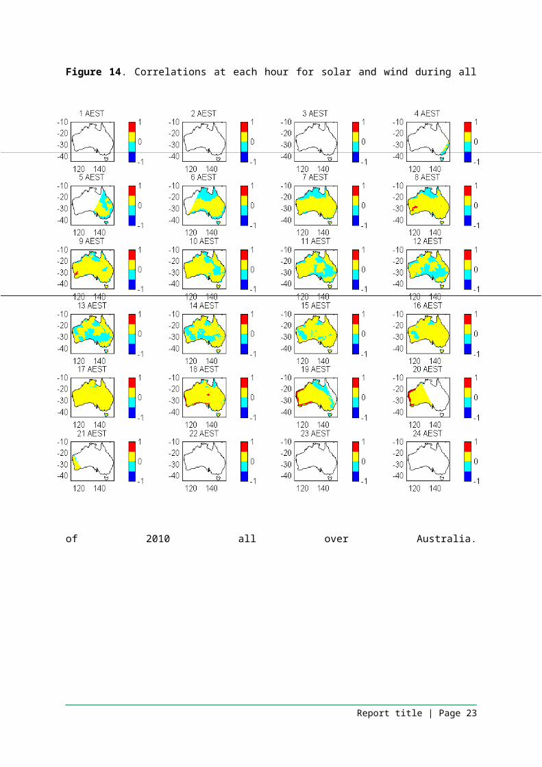
We were interested in identifying times of day where we were more likely to see correlations between wind and solar. These changes would be identified usually along the coast with on-shore or off-shore breezes. Figure 14 breaks the correlations down by hour over all 2010, all results presented are in Australian Eastern Standard Time (AEST). Hourly correlations of wind and solar for the whole year were computed after constructing time series of wind and solar flux for each hour for the whole year, and then correlating them. The question we were asking is that within each hour for the whole year, how well did solar and wind complement each other? This accounts for the variability at each hour for the whole year. In the western part of Australia we can see that correlations exist between wind and solar in the middle of the day, implying we should be seeing output from both wind and solar, we see these strong correlations again at night, which leads to the conclusion that during this time both wind and solar have low output. We also see a higher chance of anti-correlation across the continent between wind and solar throughout the days. This would imply co-locating both technologies and distributing them across the continent would maximise output from renewables.To investigate site specific synergies a region of interest was selected (near the Capital Wind farm), and correlations of wind/solar energy flux and NSW energy demand were plotted. This location was chosen as the Capital wind farm already exists in that location, as well as a PV demonstration plant. Figure 15 shows correlations at each hour during all of 2010 near the Capital Wind Farm. The morning and afternoons show weak anti-correlations of wind and solar. Demand is positively


correlated with solar energy in the afternoon, however, demand did not correlate well with wind energy over 2010. This could also be due to the variability in hourly data.Figure 16 a) shows a breakdown of daily correlations of wind-solar, b) wind-demand and c) solar-demand for all of 2010. Note that on 76% of days during all of 2010, wind and solar supplemented each other (correlations more than 0.5), whereas with 10% of all days in 2010 wind and solar complemented each other. On 85% of days in 2010 the energy demand and wind were positively correlated, whereas the energy demand and solar were 100% positively correlated, except the correlations went down during winter. A hybrid wind-solar system is highly feasible at this location.


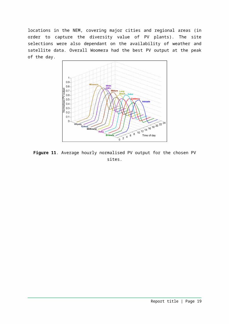
Figure 14. Correlations at each hour for solar and wind during all of 2010 all over Australia.


Figure 15. Correlations at each hour for wind-solar, wind-demand and solar-demand during all of 2010 near the Capital Wind Farm.

Figure 16. Daily correlations of a) wind-solar, b) wind-demand and c) solar-demand for 2010.


Manage high levels of solar penetration, with and without wind generators, under conditions of network stressWith increasing levels of integration of solar Photovoltaic (PV) systems in electricity networks, it is important for them to continue to prove their effectiveness in the energy market. Integrating energy storage into the system is seen as a potential solution, as storing the renewable power when it is generated and supplying it to the local load, or to the grid when it is required, can perform a vital function of time shifting. This can potentially increase the value of a renewable energy system as well as solves some of the network issues. This work studied both financial and technological benefits of adding storage to existing rooftop PV systems, focusing on residential households in Sydney.Customer load data in the Endeavour Energy Network Area was obtained for a random selection of ten Sydney households. A MATLAB model was developed to investigate how adding varying capacities of PV and battery systems would affect the resulting network load, annual electricity consumption and hence the economic viability, for various tariff regimes and structures. The PV system models were based on Bureau of Meteorology (BOM) one-minute solar data from the nearest station at Wagga Wagga. This study concluded that the benefits of a PV rooftop system can be increased by incorporating storage, with the added benefit that storage can also significantly impact the network peak load, which can lead to deferral of network augmentation.

Comparing output from solar energy systems with electricity loads on the distribution and transmission networks.The aim of this work was to identify and quantify the financial impacts of Air Conditioning (AC), Photovoltaics (PV), PV with battery storage, Solar Water Heaters (SWH’s) and energy efficiency in the Australian National Electricity Market (NEM). We were interested in also investigating the way in which the impacts of different tariffs could help customers reduce their demand peaks and hence reduce the costs imposed on other customers. Therefore, an assessment was carried out to investigate the impacts on transmission network service providers (TNSPs), distribution network service providers (DNSPs), retailers, the households that use these technologies, and households that do not. We have assumed that 20% of households have installed the above technologies. The two tariffs included in this assessment are: Energy Australia’s regulated ‘Domestic All Time’ tariff, Energy Australia’s PowerSmart Home Time of Use (TOU) tariff, and a custom designed residential Demand charge tariff.The longer term cost impacts due to increases in demand peaks have two different implications for TNSP’s and DNSP’s. For TNSP’s an increased demand peak that occurs during the network wide peak results in consideration of increasing the size of the network. For DNSP’s an increased demand peak that occurs during the local feeder peak implies that the size of the local network may need to be increased.The load data used for this work consisted of annual load profile and PV generation based on half hourly data from 61 houses for the period 1 July 2009 to 30 June 2010, in Blacktown, NSW. The NSW peak demand for 2009/10 was in summer. The Load and PV Output on the Peak Demand Day for the Sample Houses on Tues 12 Jan 2010, as well as the summer average load is shown in Figure 17. What was interesting about this peak was it occurred earlier in the day than the average peak, a consequence of air conditioner usage. Networks are built to meet the anticipated annual peak, and so only changes to this peak affect the required size of the network. What is most important for this


aspect is when the demand peak occurs. Transmission networks have a load profile that reflects the aggregated state-wide demand from all users – industrial, commercial and residential. It was found that PV reduces the demand peaks brought on by the increase due to AC. All demand peaks seen by networks can reduce or increase demand and are dependent on a number of factors. PV’s ability to reduce costs is entirely dependent on its ability to reduce demand at the annual peak. The peak demand reduction modelling was based on actual data where 20% of the PV’s rated capacity was available during the distribution network peak. The amount of PV capacity available on different distribution network peaks can vary from 11.8% to 48.5%.

Figure 17. Load and PV Output on the Peak Demand Day for the Sample Houses on Tues 12 Jan 2010, as well as the average summer load.

TransferabilityThe forecasting work carried out in this project can be applied to the Australian Solar Energy Forecasting Scheme (ASEFS), and assist AEMO in understanding how the weather impacts output from the various renewable technologies.

Conclusion and next stepsThis project looked at new techniques and applying known models to the forecasting challenge, and ways to understand how solar and wind can smoothly integrate into the electricity grid. The project brought together Australian researchers and industry and found,

Using TAPM, The results revealed that the resolution of 45 km had the lowest Root Mean Square Error (RMSE). This means that variations on scales less than 45 km cannot be captured by the model properly. Furthermore, correcting the 45 km modelled GHI for clear-sky errors improved the accuracy of the model and reduced the RMSE, Mean Absolute Error (MAE) and Mean Bias Error (MBE) on average by maximum 16 %, 26 % and 84 % respectively. In comparing the performance of WRF to TAPM, if looking at RMSE alone, did not really improve with a finer resolution. The coarser resolution often was the most accurate, even though differences between the coarser and fine resolution only differed by 5 – 15 Wm-2 for all sky conditions, for both TAPM and WRF respectively. Greater differences were seen in MBE for WRF than TAPM.


Overall both models had their advantages when forecasting solar radiation. WRF however has the added benefit of being able to forecast DNI, which is important when investigating both PV and Concentrated Solar Technologies (CST).

The CARDS model for short term forecasting has been tested against the best in the literature, performing very well. Short term work also provided a model output statistics (MOS) method of improving solar irradiance forecasts from the Weather Research and Forecasting (WRF) Model. The impacts of deliverable power, with incorporating high solar penetration and looking at correlations between PV and Solar and their match with demand has shown that solar is a better match to demand than wind, and synergies between PV and wind need to be made on a site specific basis as weather varies so much within a state.

Comparing output from solar energy systems with electricity loads on the distribution and transmission networks concluded that the benefits of a PV rooftop system can be increased by incorporating storage, with the added benefit that storage can also significantly impact the network peak load, which can lead to deferral of network augmentation. We also found that PV reduces the transmission network peak, and hence reduces network augmentation costs for all customers to a greater extent.

Significant benefit came from the collaboration, with knowledge sharing occurring at yearly meetings.This work can be taken further and will continue within ASEFS, where the methods applied here will be modified for distributed forecasting. Hybrid forecasting will become more necessary as we start to see solar and wind co-located. Methods need to be identified on the best way to forecast for a hybrid system. Our project partners are continuing their work on assessment by combining a wind and solar map for co-location of hybrid systems.


Lessons LearntLessons Learnt Report: TechnicalProject Name: Forecasting and Characterising Grid Connected Solar Energy and Developing Synergies with WindKnowledge Category: Technical<Choose anItem>Knowledge Type:

Outputs

Technology Type: Solar PV<Choose anitem>State/Territory:

NSW

Key learningThe key collaborators covered a range of expertise in forecasting, weather models, statistics, integration of renewables and market mechanisms. This ensured a clear link of development between the weather and solar and wind resource, siting and implications to large scale and distributed technology, as well as the network and market mechanisms associated with integration of solar technologies. These set up the basis for determining a forecasting system for solar PV. The expertise allowed good progress to be made and knowledge development in the solar resource and forecasting area.

Implications for future projectsCollaborative projects involving researchers with different skill bases allows a greater scope to be covered, giving a more holistic view of the area of research. Planning is key for the success of a project.

Knowledge gapDistributed forecasting requires a very different approach to the solar forecasting problem than what has been covered for large scale generation. Some of the techniques used in this project can be adapted to forecasting distributed generation.

BackgroundObjectives or project requirementsThe need to actively and effectively manage large scale penetration of renewable energy technologies requires new advances in meteorology and forecasting methods that will facilitate the uptake of these resources in electricity networks, enhancing their value as a deliverable power technology. Thus the objectives of this research project are to:(i) Develop metrics for deciding suitability of a site for any given configuration of solar and wind technology by examining the characteristics of weather variability – data analysis and characterising variability. Results from this will feed into Objective (ii).(ii) Develop a real-time forecasting scheme for the prediction of energy output from solar technologies in line with National Electricity Market (NEM) dispatch timeframes. This can be used to more efficiently manage resource fluctuations. Technologies important for this study include PV,

24

STE and wind energy, the latter due to prior knowledge of wind energy forecasting and deployment techniques which will allow solar-wind synergies to be analysed.(iii) To report on how solar technologies interact with Australian electricity and gas networks – output from this objective has particular relevance to any participant in the National Electricity Market, with forecasting of STE also being of relevance to gas markets. (iv) Develop strategies to manage high levels of solar penetration under various network conditions.

Process undertakenThis project brought together researchers from the University of New South Wales, University of South Australia, Bureau of Meteorology, Australian PV Association and Epuron. This team encompassed a range of researchers and stakeholder groups and benefitted from this wide area of expertise. This collaboration was able to deliver on this project through sharing of data, ideas and analysis of results.


Documents

Table of Contents · Web viewThe solar radiation also has different components, Global Horizontal Irradiance (GHI), which is what Photovoltaic (PV) technology converts into power,