Embed Size (px)
Citation preview
Daniele Bortoluzzi Control Systems for the Mitigation of Footbridge Vibrations
I
Table of Contents
Introduction 1
Chapter 1 State of the art for the design of footbridges............................................... 3
1.1 Scientific papers ............................................................................................... 4
1.1.1 Footbridge Dynamics ............................................................................. 4
1.1.2 Human Induced Vibration (HIV) ........................................................... 8
1.2 Recommendations and prescriptions ................................................................ 8
1.3 References ...................................................................................................... 15
Chapter 2 Design requirements and performance satisfaction .................................. 19
2.1 Dynamics of the footbridges design and structural health monitoring ........... 20
2.1.1 Governing relations .............................................................................. 20
2.1.2 Structural Health Monitoring ............................................................... 32
2.2 Comfort for footbridges: codes and literature overview ................................. 39
2.3 Pedestrian Timber Bridge: a new construction way. Introduction to the
structures under study ................................................................................................. 44
2.4 References ...................................................................................................... 50
Chapter 3 Experimental campaign and numerical modeling .................................... 55
3.1 Experimental campaign .................................................................................. 55
3.1.1 “Tesa” footbridge experimental campaign ........................................... 56
3.1.2 “Trasaghis” footbridge experimental campaign ................................... 64
3.2 Cable-stayed system: “Tesa” footbridge FE Model ........................................ 70
3.2.1 Design data and numerical model definition ........................................ 70
3.2.2 FE Model refinement and validation .................................................... 76
3.3 FE Model of the “Trasaghis” footbridge ........................................................ 78
3.3.1 Project data and numerical model definition ........................................ 78
3.3.2 FE Model refinement and validation .................................................... 85
3.4 References ...................................................................................................... 93

Daniele Bortoluzzi Control Systems for the Mitigation of Footbridge Vibrations
II
Chapter 4 Modeling the main actions ....................................................................... 97
4.1 Wind action .................................................................................................... 98
4.2 Human induced vibration source ................................................................. 106
4.2.1 Crowd Load Model (CLM) ............................................................... 107
4.3 Time-histories simulation ............................................................................ 114
4.3.1 Wind velocity field ............................................................................ 114
4.3.2 Crowd Load Model: numerical simulation and validation ................ 118
4.4 References .................................................................................................... 124
Chapter 5 Model order reduction (MOR) ............................................................... 127
5.1 MOR background ........................................................................................ 128
5.2 Structural response ....................................................................................... 133
5.3 MOR accuracy ............................................................................................. 142
5.4 References .................................................................................................... 144
Chapter 6 Control solutions .................................................................................... 147
6.1 Passive control solutions .............................................................................. 149
6.2 Semiactive control solutions ........................................................................ 165
6.3 Active control solutions ............................................................................... 180
6.4 References .................................................................................................... 191
Chapter 7 Conclusions ............................................................................................ 193
Appendix A: Technical details for the two footbridges used as case studies ............... 195
A.1 Trasaghis footbridge .................................................................................... 195
A.2 Tesa footbridge ............................................................................................ 208
A.3 References ................................................................................................... 219
Appendix B: A standard model for the single pedestrian walking and running .......... 221
B.1 Dynamic behaviour of a single pedestrian ................................................... 221
B.2 References ................................................................................................... 229
Appendix C: Overview of some existing codes and guidelines ................................... 231
C.1 ISO 10137 .................................................................................................... 231
Daniele Bortoluzzi Control Systems for the Mitigation of Footbridge Vibrations
III
C.2 Fib-buletin 32 ............................................................................................... 233
C.3 BS 5400 ........................................................................................................ 236
C.4 Sétra-AFGC .................................................................................................. 237
C.5 The comfort level in existing recommendations .......................................... 242
C.6 References ................................................................................................... 244
Appendix D: Crowd Load Model (CLM): experimental data set ................................. 247
D.1 Time-Frequency analysis of the signals: theoretical background ................. 247
D.2 Experimental data analysis .......................................................................... 251
D.3 References ................................................................................................... 266
Acknowledgements ...................................................................................................... 269

Daniele Bortoluzzi Control Systems for the Mitigation of Footbridge Vibrations
IV
Daniele Bortoluzzi Control Systems for the Mitigation of Footbridge Vibrations
V
Table of Figures and Tables
Figure 1.1. The Millennium Bridge. ................................................................................. 3 Figure 1.1.1. Vibration comfort criteria for footbridges in case of human induced
vibrations [8]. ................................................................................................................... 5 Figure 1.1.2. Monitoring system of the Pedro Gómez Bosque footbridge [12]. ............... 6 Figure 1.1.3. On the left: general view of the footbridge. On the right: testing under
human induced vibration [13]. ......................................................................................... 6 Figure 1.1.4. Active control scheme [19]. ........................................................................ 7 Figure 1.2.1. Peak of tolerable acceleration for high range of frequencies (f >> 1 Hz)
([27] and [28]). ............................................................................................................... 10 Figure 1.2.2. Peak of tolerable acceleration for low range of frequencies (f < 1 Hz).
Values are plotted in terms of root-mean-square of the acceleration. To compare these
result with the ones proposed in Figure 1.2.1, multiply these values by 20.5 ([29]-[31]).
........................................................................................................................................ 10 Figure 1.2.3. Summary of human exposure to acceleration. Peak accelerations versus
frequencies [32]. ............................................................................................................. 11 Figure 1.2.4. Peak acceleration criteria proposed by [35] and [26]. ............................... 12 Figure 1.2.5. Structural safety criteria for frequencies range up to 50 Hz [41]. ............. 13 Figure 1.2.6. General peak acceleration criteria [43]. .................................................... 14 Figure 2.1.1. Schematic representation of a 1-DOF system. .......................................... 21 Figure 2.1.2. Dynamic parameter trend for specific value of the critical damping. ....... 23 Figure 2.1.3. Free oscillation of a 1-DOF system with different value of damping. ...... 24 Figure 2.1.4. Oscillation of a 1-DOF system – divergences induced by a “negative”
damping. ......................................................................................................................... 25 Figure 2.1.5. Representation of the “logarithmic decrement method”. .......................... 26 Figure 2.1.6. Representation of the “bandwidth method”. ............................................. 26 Figure 2.1.7. Schematic representation of a n-DOF system. .......................................... 26 Figure 2.1.8. Modal superposition approach applied to a 2-DOF system. ..................... 32 Figure 2.1.9. SHM architecture applied to a bridge [12]. ............................................... 34 Figure 2.1.10. Example of proposed rehabilitation planning based on the Ultimate Limit
Strength [13]. .................................................................................................................. 34 Figure 2.1.11. SHM for bridge. Typical flowchart [16]. ................................................ 36 Figure 2.1.12. SHM for bridge. Typical flowchart [25]. ................................................ 37 Figure 2.2.1. Building vibration z-axis base curve for acceleration (foot-to-head
vibration direction) [33]. ................................................................................................ 41
Daniele Bortoluzzi Control Systems for the Mitigation of Footbridge Vibrations
VI
Figure 2.2.2. Building vibration z-axis base curve for acceleration (foot-to-head
vibration direction) [33]. ................................................................................................ 42 Figure 2.2.3. Methodology flowchart proposed by Sétra-AFGC [36]. .......................... 44 Figure 2.3.1. “Trasaghis” footbridge. ............................................................................ 45 Figure 2.3.2. “Trasaghis” footbridge. View of the pillars. ............................................. 45 Figure 2.3.3. View from the bottom of the “Trasaghis” footbridge on the left. Zoom on
the structural resistant scheme of the deck on the right. ................................................ 46 Figure 2.3.4. General view of the “Tesa” footbridge. .................................................... 46 Figure 2.3.5. “Tesa” footbridge. Satellite view of the location. ..................................... 46 Figure 2.3.6. View of the pillar on the left; detail of the connection between cable and
deck on the right. ........................................................................................................... 47 Figure 2.3.7. View of the structural scheme of the “Tesa” footbridge deck. ................. 47 Figure 2.3.8. Tynset bridge, Norway [40]. .................................................................... 48 Figure 2.3.9. Cosumnes River Bridge, California (USA) [41]. ..................................... 48 Figure 2.3.10. Goodpasture Covered Bridge. Lane County, Oregon (USA) [42]. a)
lateral view; b) frontal view. .......................................................................................... 49 Figure 2.3.11. Goodpasture Covered Bridge. Lane County, Oregon (USA) [43]. ......... 49 Figure 2.3.12. Lejonstroms Bridge. Skelleftea, Sweden [44]. ....................................... 50 Figure 3.1.1. Example of the tri-axial accelerometer posed over the deck. ................... 56 Figure 3.1.2. Example of the wireless station unit (WSU) employed for the data
acquisition-transmission. ............................................................................................... 57 Figure 3.1.3. Sensors equipment configuration during the in situ tests. ........................ 57 Figure 3.1.4. Sensors WSa1 during the in situ tests. ...................................................... 58 Figure 3.1.5. Sensors WSa2 during the in situ tests. ...................................................... 58 Figure 3.1.6. Sensors WSa3 during the in situ tests. ...................................................... 58 Figure 3.1.7. “Tesa” footbridge – picture during test B2. .............................................. 59 Figure 3.1.8. Acceleration along the Z axis recorded by WSa2 – duration 25 sec –
sampling rate 100 Hz – November 7, 2013 @ 2.12 pm – air temperature 15°C. .......... 60 Figure 3.1.9. Acceleration along Z axe recorded (160 sec) by WSa2 – sampling rate 100
Hz – November 7, 2013 @ 2.55 pm – air temperature 15°C. ........................................ 60 Figure 3.1.10. Data processing – acceleration acquired by WAa1 during the test A along
Y transversal axis. a) FFT; b) STFFT............................................................................. 61 Figure 3.1.11. Data processing – acceleration acquired by WAa1 during the test A along
Y transversal axis. a) WA. .............................................................................................. 62 Figure 3.1.12. Data processing by using SSI – acceleration acquired by WAa1 during
the test A along Y transversal axis. a) mode I (f=1.30 Hz); b) mode III (f=2.85 Hz). .... 63 Figure 3.1.13. The tri-axial accelerometer connected with a wireless sensor unit (WSU)
posed over the deck. ...................................................................................................... 64
Daniele Bortoluzzi Control Systems for the Mitigation of Footbridge Vibrations
VII
Figure 3.1.14. Example of the Kinemetric EPISENSOR uni- and tri- axial accelerometer
employed during the experimental campaigns. .............................................................. 65 Figure 3.1.15. Sensors configuration for the two experimental campaign (November 30,
2012 and May 12, 2013). ................................................................................................ 66 Figure 3.1.16. Periodograms of the signals recorded at position 3 (P#3): from the top to
bottom, one sees the elaboration of the signals (along direction Y) collected in
November, in the early morning of May 12, 2013 and in the late morning of the same
day. The number of points in the temporal window of the signal is 2170. ..................... 67 Figure 3.1.17. Periodograms of the signals recorded at position 3 (P#3): from the top to
bottom, one sees the elaboration of the signals (along direction Z) collected in
November, in the early morning of May 12, 2013 and in the late morning of the same
day. The number of points in the temporal window of the signal is 2170. ..................... 68 Figure 3.1.18. Periodograms of the signals recorded at position 7 (P#7): FFT along
direction Y. ..................................................................................................................... 69 Figure 3.1.19. Periodograms of the signals recorded at position 7 (P#7): FFT along
direction Z - data collected in May 12, 2013. ................................................................. 70 Figure 3.2.1. View of the numerical model implemented in MARC Mentat2010. ........ 71 Figure 3.2.2. Detail of the kinematics boundary condition below the mains GLT beams.
On the left picture from field; on the right the implemented boundary on the numerical
model. ............................................................................................................................. 73 Figure 3.2.3. Detail of the kinematics boundary condition at the base of the pillars. On
the left picture from field; on the right the implemented boundary on the numerical
model. ............................................................................................................................. 74 Figure 3.2.4. Detail of the kinematics boundary condition at the base of the pillars. On
the left picture from field; on the right the implemented boundary on the numerical
model. ............................................................................................................................. 74 Figure 3.2.5. Above: lateral view of the numerical model; below: view from the above.
........................................................................................................................................ 75 Figure 3.2.6. Frontal view of the numerical model. ....................................................... 75 Figure 3.2.7. 3-D view of the numerical model. ............................................................. 75 Figure 3.2.8. View of the deck. On the left 3-D view; on the right cross-section view. . 76 Figure 3.2.9. FFT – acceleration acquired by WAa1 during the test A along the Y axis.77 Figure 3.2.10. Mode I – prevalent motion along the transversal direction Y. FEM
dynamic modal analysis performed in MARC Mentat2010 – f = 1.28 Hz. .................... 77 Figure 3.3.1. View of the numerical model implemented in MARC Mentat2010. ........ 79 Figure 3.3.2. Detail of the kinematics boundary condition at the base of the pillars. On
the left picture from field; on the right the implemented boundary on the numerical
model. ............................................................................................................................. 81
Daniele Bortoluzzi Control Systems for the Mitigation of Footbridge Vibrations
VIII
Figure 3.3.3. Detail of the kinematics boundary condition at the base of the stays. On
the left picture from field; on the right the implemented boundary on the numerical
model. ............................................................................................................................ 81 Figure 3.3.4. Detail of the kinematics boundary condition for the GLT beams. On the
left picture from field; on the right the implemented boundary on the numerical model.
....................................................................................................................................... 82 Figure 3.3.5. Above: lateral view of the numerical model; below: view from the above.
....................................................................................................................................... 83 Figure 3.3.6. Frontal view of the numerical model. ....................................................... 83 Figure 3.3.7. 3-D view of the numerical model. ............................................................ 84 Figure 3.3.8. View from the bottom of the deck. On the left picture from field; on the
right the implemented boundary on the numerical model. ............................................ 84 Figure 3.3.9. View of the deck. On the left 3-D view; on the right cross-section view. 84 Figure 3.3.10. View of the steel pillars and stays systems. On the left 3-D view; on the
right cross-section view. ................................................................................................ 85 Figure 3.3.11. Partial numerical of the steel pillars and stays implemented in MARC
Mentat2010. ................................................................................................................... 85 Figure 3.3.12. Mode I – local mode related to the prevalent vertical motion of the stays.
a) FFT of the experimental data (Campaign of May, 2013 – position P#7) – f =
1.08±1.11 Hz; b) FEM dynamic modal analysis performed in MARC Mentat2010 – f =
1.06 Hz. ......................................................................................................................... 88 Figure 3.3.13. Mode II – local mode related to the prevalent horizontal/transversal
motion of the stays. a) FFT of the experimental data along Y (Campaign of May, 2013 –
position P#7) – f = 1.31±1.43 Hz; b) FFT of the experimental data along Y (Campaign
of May, 2013 – position P#1) – f = 1.37 Hz. ................................................................. 89 Figure 3.3.14. Mode II – local mode related to the prevalent horizontal/transversal
motion of the stays. a) FFT of the experimental data along Z (Campaign of May, 2013 –
position P#1) – f = 1.5 Hz; b) FEM dynamic modal analysis performed in MARC
Mentat2010 – f = 1.41 Hz. ............................................................................................. 90 Figure 3.3.15. Mode III – global “pseudo” torsional mode of the deck. a) FFT of the
experimental data along Y (Campaign of May, 2013 – position P#7) – f = 1.95 Hz; b)
FFT of the experimental data along Y (Campaign of May, 2013 – position P#1) – f =
1.97 Hz. ......................................................................................................................... 91 Figure 3.3.16. Mode III – global “pseudo” torsional mode of the deck. a) FFT of the
experimental data (Campaign of May, 2013 – position P#3) – f = 1.74±1.95 Hz; b) FFT
of the experimental data along Y (Campaign of May, 2013 – position P#3) – f =
1.74±1.95 Hz. ................................................................................................................ 92 Figure 3.3.17. Mode III – global “pseudo” torsional mode of the deck. FEM dynamic
modal analysis performed in MARC Mentat2010 – f = 1.96 Hz. .................................. 93
Daniele Bortoluzzi Control Systems for the Mitigation of Footbridge Vibrations
IX
Figure 4.1.1. Global reference frame. ............................................................................. 99 Figure 4.1.2. Example of “mean” wind velocity (U) trend for three different case of
roughness [8]. ................................................................................................................. 99 Figure 4.1.3. Flowchart for the wind velocity field simulation. ................................... 106 Figure 4.2.1. Grid of nodes for the simulation. ............................................................ 108 Figure 4.2.2. Local frame system for the k-th node. ..................................................... 110 Figure 4.2.3. Spatial configuration of the crowd model implemented. ........................ 111 Figure 4.2.4. Classical model of moving loads. Deterministic approach. An example of
two consecutive time steps. .......................................................................................... 111 Figure 4.2.5. Flowchart for the CLM simulation. ......................................................... 112 Figure 4.2.6. Above: experimental set-up; below: walking test of six person
configuration. ............................................................................................................... 113 Figure 4.3.1. Grid of nodes for wind velocity field simulation. ................................... 114 Figure 4.3.2.Wind velocity components along the x1 and x3 axes as simulated for node:
a) n1, b) n19. ................................................................................................................ 115 Figure 4.3.3.Force components along the x1 and x3 axes for node: a) n8, b) n22 and c)
n23. ............................................................................................................................... 117 Figure 4.3.4. a) Grid of nodes for the simulation; b) example of the deck nodal grid
implemented in MARC Mentat2010. ........................................................................... 118 Figure 4.3.5. Steady component of the force over the simulation grid. ........................ 119 Figure 4.3.6. 3-D plot of the "barrel dented" function over the nodes of the simulation
grid. .............................................................................................................................. 119 Figure 4.3.7. Step 1 – simulated force files by the proposed CLM model. .................. 120 Figure 4.3.8. Step 2 – simulated force files by the proposed CLM model. .................. 120 Figure 4.3.9. Step 3 – simulated force files by the proposed CLM model. .................. 121 Figure 4.3.10. Example of the simulated forces implemented in MARC Mentat2010. 122 Figure 4.3.11. Time-frequency plots from the data taken by sensor WSa2 along axis Y
(transversal). a) data acquired in situ; b) data from the numerical simulation. ............. 122 Figure 4.3.12. Time-frequency plots from the data taken by sensor WSa2 along axis Z
(gravity) a) data acquired in situ and filtered at 2.50 Hz; b) data from the numerical
simulation. .................................................................................................................... 123 Figure 5.1. MOR: graphical representation [4]. ........................................................... 128 Figure 5.1.1. MOR: visual representation [11]. ............................................................ 132 Figure 5.2.1. “Light” FEM implemented in MARC Mentat2010 environment............ 133 Figure 5.2.2. Dynamic modal comparison of the “Trasaghis” footbridge FEM: mode I.
a) “Light” FEM f = 1.22 Hz; b) “Full” FEM f = 1.06 Hz. ........................................... 134 Figure 5.2.3. Dynamic modal comparison of the “Trasaghis” footbridge FEM: mode II.
a) “Light” FEM f = 1.32 Hz; b) “Full” FEM f = 1.41 Hz. ........................................... 135
Daniele Bortoluzzi Control Systems for the Mitigation of Footbridge Vibrations
X
Figure 5.2.4. Dynamic modal comparison of the “Trasaghis” footbridge FEM: mode III.
a) “Light” FEM f = 2.40 Hz; b) “Full” FEM f = 1.96 Hz. ........................................... 136 Figure 5.2.5. Dynamic modal comparison of the “Trasaghis” footbridge FEM: mode IV.
a) “Light” FEM f = 1.87 Hz; b) “Full” FEM f = 2.83 Hz. ........................................... 137 Figure 5.2.6. Dynamic modal comparison of the “Trasaghis” footbridge FEM: mode V.
a) “Light” FEM f = 3.47 Hz; b) “Full” FEM f = 3.07 Hz. ........................................... 138 Figure 5.2.7. Hankel Singular Values – State Contributions. ...................................... 139 Figure 5.2.8. Gird of nodes for the “light” numerical model of the “Trasaghis”
footbridge..................................................................................................................... 139 Figure 5.2.9. Fluctuating part of the simulated wind velocity for the node 5. a) Y
component; b) Z component. ....................................................................................... 140 Figure 5.2.10. Wind forces for the node 5. a) Y component; b) Z component. ........... 141 Figure 5.2.11. Dynamic response of the “light” FEM under the simulated wind loads –
node 3. Displacement along Y and Z axes. .................................................................. 141 Figure 5.2.12. Dynamic response of the “light” FEM under the simulated wind loads –
node 3. Accelerations along Y and Z axes. .................................................................. 142 Figure 5.3.1. Comparison among “light” FEM and the implemented MOR models in
terms of displacements along Y and Z axes – node 3. a) MOR 145 states; b) MOR 114
states. ........................................................................................................................... 143 Figure 5.3.2. Comparison among “light” FEM and the implemented MOR models in
terms of displacements along Y and Z axes – node 3 - MOR 84 states. ...................... 144 Figure 6.1. Scheme of a Passive Control System [2]. .................................................. 148 Figure 6.2. Scheme of an Active Control System [2]. ................................................. 148 Figure 6.1.1. 3-D view of the numerical model of the “Trasaghis” footbridge
implemented in Marc MENTAT2010. ........................................................................ 153 Figure 6.1.2. View of the implemented TMDs solution on “Trasaghis” footbridge. In
particular TMD1 and TMD3 hung on the tubular elements in the l.h.s. of the footbridge,
while TMD2 and TMD4 are hanged on the tubular elements in the r.h.s. ................... 154 Figure 6.1.3. Above: Lateral view of the location of the i-th TMD. Below: cross-section
of the i-th TMD. ........................................................................................................... 157 Figure 6.1.4. Grid of nodes. ......................................................................................... 158 Figure 6.1.5. Time histories response before and after mounting the passive control
system (“TMD_A”) designed. Acceleration responses for the node n22 along x1 (a) and
x3 (b), respectively. ..................................................................................................... 160 Figure 6.1.6. Time histories response before and after mounting the passive control
system (“TMD_A”) designed. Acceleration responses along x1 at the node n8. ....... 161 Figure 6.1.7. Time histories response before and after mounting the passive control
system (“TMD_A”) designed. Displacement responses for the node n22 along x1 (a)
Daniele Bortoluzzi Control Systems for the Mitigation of Footbridge Vibrations
XI
and x3 (b), respectively. The response of the node n8 is meaningful due to the stiffness
of the deck. ................................................................................................................... 162 Figure 6.1.8. Response spectra as obtained from the acceleration responses along x1 (a)
and x3 (b) at the node n22; and (c) from the acceleration response along x1 at the node
n8, before and after the installation of the passive control system (TMD_A). ............. 164 Figure 6.1.9. Response spectra as obtained from the acceleration responses along x1 (a)
and x3 (b) at the node n22, before and after the installation of the passive control system
(TMD_A). .................................................................................................................... 165 Figure 6.2.1. Time history of the relative displacement for the node of TMD2 along x1
direction a), and x3 direction b). ................................................................................... 168 Figure 6.2.2. View of the TMD_C of the “Trasaghis” footbridge. .............................. 169 Figure 6.2.3. Time histories of the accelerations (a) along direction x1 and (b) along
direction x3 obtained for node n22 under the semiactive control scheme TMD_As3. .. 172 Figure 6.2.4. Time histories of the displacements (a) along direction x1 and (b) along
direction x3 obtained for node n22 under the semiactive control scheme TMD_As3. .. 173 Figure 6.2.5. Time histories of the accelerations (a) along direction x1 and (b) along
direction x3 obtained for node n8 under the semiactive control scheme TMD_As3. .... 174 Figure 6.2.6. Time histories of the displacements (a) along direction x1 and (b) along
direction x3 obtained for node n8 under the semiactive control scheme TMD_As3. .... 175 Figure 6.2.7. Time histories of the accelerations (a) along direction x1 and (b) along
direction x3 obtained for node n22 under the semiactive control scheme TMD_ Bs1. . 176 Figure 6.2.8. Time histories of the displacements (a) along direction x1 and (b) along
direction x3 obtained for node n22 under the semiactive control scheme TMD_ Bs1. . 177 Figure 6.2.9. Time histories of the accelerations (a) along direction x1 and (b) along
direction x3 obtained for node n8 under the semiactive control scheme TMD_ Bs1. ... 178 Figure 6.2.10. Time histories of the displacements (a) along direction x1 and (b) along
direction x3 obtained for node n8 under the semiactive control scheme TMD_Bs1. .... 179 Figure 6.3.1. Scheme of the control forces implemented for the “Trasaghis” footbridge.
...................................................................................................................................... 183 Figure 6.3.2. Time history of the control forces – node 3. a) MOR 145 states; b) MOR
114 states; c) MOR 84 states. ....................................................................................... 184 Figure 6.3.3. Active control solution for the “Trasaghis” footbridge - model MOR 145
states: comparison of uncontrolled vs. controlled. Response of: a) Displacements along
Y and Z axes – node 3; b) Accelerations along Y and Z axes (zoom between 10 to 20
sec) – node 3. ................................................................................................................ 185 Figure 6.3.4. Active control solution for the “Trasaghis” footbridge - model MOR 145
states: comparison of uncontrolled vs. controlled. Response of: a) Displacements along
Y and Z axes – node 5; b) Accelerations along Y and Z axes (zoom between 10 to 20
sec) – node 5. ................................................................................................................ 186
Daniele Bortoluzzi Control Systems for the Mitigation of Footbridge Vibrations
XII
Figure 6.3.5. Active control solution for the “Trasaghis” footbridge - model MOR 114
states: comparison of uncontrolled vs. controlled. Response of: a) Displacements along
Y and Z axes – node 3; b) Accelerations along Y and Z axes (zoom between 10 to 20
sec) – node 3. .............................................................................................................. 187 Figure 6.3.6. Active control solution for the “Trasaghis” footbridge - model MOR 114
states: comparison of uncontrolled vs. controlled. Response of: a) Displacements along
Y and Z axes – node 5; b) Accelerations along Y and Z axes (zoom between 10 to 20
sec) – node 5. ............................................................................................................... 188 Figure 6.3.7. Active control solution for the “Trasaghis” footbridge - model MOR 84
states: comparison of uncontrolled vs. controlled. Response of: a) Displacements along
Y and Z axes – node 3; b) Accelerations along Y and Z axes (zoom between 10 to 20
sec) – node 3. ............................................................................................................... 189 Figure 6.3.8. Active control solution for the “Trasaghis” footbridge - model MOR 84
states: comparison of uncontrolled vs. controlled. Response of: a) Displacements along
Y and Z axes – node 5; b) Accelerations along Y and Z axes (zoom between 10 to 20
sec) – node 5. .............................................................................................................. 190 Figure A.1.1. Chorography at scale 1:25000: the map shows the lake and the emissary
channel. The red circle indicates the bridge location. .................................................. 196 Figure A.1.2. A general view of the “Trasaghis footbridge”. ...................................... 196 Figure A.1.3. Technical drawings of the footbridge. ................................................... 197 Figure A.1.4. Details of the main GLT beams: a) view during the construction stage; b)
details of the joint connection. ..................................................................................... 198 Figure A.1.5. Details of the deck cross-section resistant scheme. ............................... 199 Figure A.1.6. View from above of the structural scheme of the deck.......................... 199 Figure A.1.7. Detail of the walking table during the construction stage. ..................... 200 Figure A.1.8. Example of the structural joint connection: detail of the joint. .............. 200 Figure A.1.9. Example of the structural joint connection: connection of the lateral
section in correspondence of the steel oblique tubular element. .................................. 201 Figure A.1.10. Construction stage: assembling the central section of the footbridge. a)
before the assembly; b) during the stage. ..................................................................... 201 Figure A.1.11. A detail of the tubular steel oblique elements (left). A lateral view of the
antenna (right). ............................................................................................................. 202 Figure A.1.12. View of the upper protection system of the beam made by copper (left).
A detail of the external larch cladding (right). ............................................................. 202 Figure A.1.13. View of the neoprene support. ............................................................. 203 Figure A.1.14. Load test stage. a) Load configuration (measure in m); b) during the test
(below). ........................................................................................................................ 204 Figure A.1.15. Measurement during the load test stage carried out. ............................ 204 Figure A.1.16. Lateral view of the Trasaghis footbridge. ............................................ 205
Daniele Bortoluzzi Control Systems for the Mitigation of Footbridge Vibrations
XIII
Figure A.1.17. Frontal view of the Trasaghis footbridge. ............................................ 205 Figure A.1.18. Detail of the structural joint between the GLT curved beam and the
oblique steel tubular element. ....................................................................................... 205 Figure A.1.19. View of the reinforced concrete foundation system. ............................ 206 Figure A.1.20. View from above of the walkway. Detail of the H-shape steel element
connection with the GLT curved beam. ....................................................................... 207 Figure A.1.21. Detail of the connection between the GLT curved beam and the concrete
foundation system. ........................................................................................................ 207 Figure A.2.1. a) Map of the location. The red circle indicates the bridge location. b)
Satellite view of the area where the footbridge is located. The red line indicates the
footbridge. .................................................................................................................... 208 Figure A.2.2. Lateral view of the timber footbridge ..................................................... 209 Figure A.2.3. Technical drawings of the footbridge. .................................................... 210 Figure A.2.4. Steel cables. ............................................................................................ 211 Figure A.2.5. Detail of the joint connection with the steel cables. Connection with
antenna (left); connection with the deck (right)............................................................ 211 Figure A.2.6. Details of the deck cross-section resistant scheme. ................................ 212 Figure A.2.7. View from the bottom of the deck. ......................................................... 212 Figure A.2.8. Detail of the neoprene support. .............................................................. 213 Figure A.2.9. Detail of the joints connection................................................................ 213 Figure A.2.10. Construction stage: assembling the central section of the footbridge. a)
Before the assembly; b) during the stage. ..................................................................... 214 Figure A.2.11. Survey operations during the load test. ................................................ 215 Figure A.2.12. Lateral view of the footbridge. ............................................................. 216 Figure A.2.13. Frontal view of the footbridge. ............................................................. 216 Figure A.2.14. Detail of the upper protection of the main GLT arcuate beams. .......... 217 Figure A.2.15. Detail of the internal support made by reinforced concrete. ................ 217 Figure A.2.16. Cross-section of the deck. .................................................................... 217 Figure A.2.17. Detail of the connection of the cable with the ground. ......................... 218 Figure A.2.18. View of the walking deck. .................................................................... 218 Figure B.1.1. Force trend due to different types of step [1].......................................... 222 Figure B.1.2. Schematic representation of the lateral forces during the motion [2]. .... 223 Figure B.1.3. Time history of the human induced force: vertical component [3]. ........ 223 Figure B.1.4. Time history of the human induced force: lateral component [3]. .......... 224 Figure B.1.5. Time history of the human induced force: longitudinal component [3]. 224 Figure B.1.6. Walking force: vertical component. Differences between three harmonics
representation for walking step frequency f=2Hz [3]. .................................................. 225
Daniele Bortoluzzi Control Systems for the Mitigation of Footbridge Vibrations
XIV
Figure B.1.7. Walking force. a) lateral component; b) longitudinal component.
Differences between four harmonics representation for walking step frequency f=2Hz
[3]. ............................................................................................................................... 226 Figure B.1.8. Running force. vertical component. Differences between three harmonics
representation for running step frequency f=3Hz [3]. .................................................. 227 Figure C.1.1. Building vibration z-axis base curve for acceleration (foot-to-head
vibration direction) [1]. ................................................................................................ 232 Figure C.1.2. Building vibration x- and y-axis base curve for acceleration (side-to-side
and back-to-chest vibration direction) [1]. ................................................................... 233 Figure C.2.1. Different scenarios of pedestrian densities [2]. ...................................... 234 Figure C.2.2. Velocity versus density of pedestrian [2]. .............................................. 234 Figure C.2.3. Dynamic amplification factor for resonant response due to sinusoidal
force moving across simple span [2]. .......................................................................... 235 Figure C.3.1. Methodology flowchart proposed by Sétra-AFGC [7]. ......................... 237 Figure C.3.2. Example of loads application: mode shape versus load direction [7]. ... 241 Figure C.3.3. factor ψ for vertical and longitudinal vibrations on the left, and for lateral
vibrations on the right [7]. ........................................................................................... 242 Figure C.3.1. Vertical critical accelerations (m/s²) versus natural frequency (Hz) by
various codes [7]. ......................................................................................................... 244 Figure D.1.1. Six persons walking. Time-frequency plots from the data recorded by
sensor WSa2 along transversal (Y) axis. a) data from right-to-left crossing; b) data from
left-to-right crossing. ................................................................................................... 249 Figure D.1.2. Six persons walking. Time-frequency plots from the data recorded by
sensor WSa2 along gravity (Z) axis. a) data from right-to-left crossing; b) data from
left-to-right crossing. ................................................................................................... 250 Figure D.2.1. Time-frequency plot from the data taken by sensorWSa2 along Y
transversal axis during test Ia. a) RtoL data ; b) LoR data ........................................... 252 Figure D.2.2. Time-frequency plots from the data taken by sensor WSa2 along Z gravity
axis during test Ia. a) RtoL data ; b) LtoR data ............................................................ 253 Figure D.2.3. Configuration of the walking test B2. .................................................... 255 Figure D.2.4. Time-frequency plots from the data recorded by sensor WSa2 along the
Y transversal axis during test Ib. a) RtoL data ; b) LtoR data. .................................... 257 Figure D.2.5. Time-frequency plots from the data recorded by sensor WSa2 along Z
gravity axis during test Ib. a) RtoL data ; b) LtoR data. ............................................... 258 Figure D.2.6. Configuration of the walking test B3. .................................................... 259 Figure D.2.7. Time-frequency plots from the data recorded by sensor WSa2 along Y
transversal axis during test Ic. a) RtoL data ; b) LtoR data. ......................................... 261 Figure D.2.8. Time-frequency plots from the data recorded by sensor WSa2 along Z
gravity axis during test Ic. a) RtoL data ; b) LtoR data. ............................................... 262
Daniele Bortoluzzi Control Systems for the Mitigation of Footbridge Vibrations
XV
Figure D.2.9. Time-frequency plots from the data recorded by sensor WSa2 along Y
transversal axis during test II. a) RtoL data ; b) LtoR data. ........................................... 264 Figure D.2.10. Time-frequency plot - WSa2 along Z gravity axis - test II. a) RtoL data ;
b) LtoR data. ................................................................................................................. 265 Figure D.2.11. Zoom between 1.00 Hz and 5.00 Hz of the singular value of spectral
density matrix. Comparison between acquisitions along transversal Y axis from WSa1
during the test B1 (solid black line) and test B2 (dashed black line) and test B3 (solid
red line). ....................................................................................................................... 266

Daniele Bortoluzzi Control Systems for the Mitigation of Footbridge Vibrations
XVI
Daniele Bortoluzzi Control Systems for the Mitigation of Footbridge Vibrations
XVII
Table 1.2.1. Acceleration limits in Eurocode 0 [24]. ........................................................ 9 Table 1.2.2. German Standard DIN 4150 [40]. .............................................................. 13 Table 1.2.3. Structural criteria: overall acceptance. ....................................................... 14 Table 2.1.1. Typical sensors employed during a SHM [12]. .......................................... 38 Table 3.1.1. “Tesa” footbridge – frequencies range from data analysis. ........................ 63 Table 3.1.2. Frequency ranges “Trasaghis” footbridge – main results. .......................... 69 Table 3.2.1. “Tesa” footbridge - numerical model: mains features. ............................... 72 Table 3.2.2. “Tesa” footbridge - numerical model: main features. ................................. 72 Table 3.2.3. “Tesa” footbridge - numerical model: materials properties. ....................... 72 Table 3.2.4. “Tesa” footbridge – frequencies comparison.............................................. 77 Table 3.3.1. “Trasaghis” footbridge - numerical model: geometry of the structural
elements. ......................................................................................................................... 79 Table 3.3.2. “Trasaghis” footbridge - numerical model: materials properties. ............... 80 Table 3.3.3. “Trasaghis” footbridge - numerical model: main features. ......................... 80 Table 3.3.4. Partial FEM - Frequency ranges for different boundary conditions for the
deck-stay link.................................................................................................................. 86 Table 3.3.5. Frequency ranges for the lowest modes of the “Trasaghis” footbridge. ..... 87 Table 3.3.6. Frequencies percentage error. Comparison between “field” and “FEM”
results. ............................................................................................................................ 87 Table 4.2.1. Walking (round trip) of six persons. ......................................................... 113 Table 4.3.1. Coordinates of the nodes for the simulation grid. ..................................... 114 Table 5.2.1. Frequencies percentage error. Comparison between “light” and “full” FEM.
...................................................................................................................................... 134 Table 5.3.1. Time consuming ....................................................................................... 142 Table 6.1.1. Masses of the structural and non-structural elements for the “Trasaghis”
footbridge. .................................................................................................................... 153 Table 6.1.2. Frequency ranges for the lowest modes of the “Trasaghis” footbridge. ... 153 Table 6.1.3. Optimum absorber parameters for TMD design [15]. .............................. 155 Table 6.1.4. Main features of the TMD_A solution. .................................................... 156 Table 6.1.5. Root-mean-square values computed on the whole duration (120 sec) of the
acceleration and displacement time histories obtained from the numerical analyses. The
peak values are also reported in italic, and they are expressed in m/s2 for the
accelerations, and in mm for the displacements. ........................................................... 158 Table 6.1.6. Root- mean-square values computed on the tails (the first 15 sec after the
event) of the of the response time histories obtained from the numerical analyses. The
peak values are also reported in italic, and they are expressed in m/s2 for the
accelerations, and in mm for the displacements. ........................................................... 159 Table 6.2.1. Root-mean-squares on the whole duration (120 sec) of the response time
histories computed from the numerical analyses carried out in a semi-active
Daniele Bortoluzzi Control Systems for the Mitigation of Footbridge Vibrations
XVIII
environment. The value in italic in each cell gives the peak value (with its sign)
expressed as m/s2 for the accelerations, and as mm for the displacements. ................. 170 Table 6.2.2. Root-mean-squares on the tail (the first 15 sec after the event) of the time
histories computed as response from the numerical analyses carried out. The value in
italic in each cell gives the starting point (with its sign) of the decay, expressed as m/s2
for the accelerations, and as mm for the displacements. .............................................. 171 Table B.1.1. Range of activities (top table). Typical values for step frequency (fs),
velocity (vs) and step length (ls) (bottom table) [1]. ..................................................... 222 Table B.1.2. Different Fourier coefficients for walking and running [4]. .................... 228 Table C.1.1. Coordination factor C(N) suggested by ISO 10137 [1]. .......................... 233 Table C.3.1.Acceleration ranges (in m/s²) for vertical vibrations proposed by Sétra-
AFGC [7]. .................................................................................................................... 239 Table C.3.2. Acceleration ranges (in m/s²) for horizontal vibrations proposed by Sétra-
AFGC. The acceleration is limited in any case to 0.10 m/s² to avoid lock-in effect [7].
..................................................................................................................................... 239 Table C.3.3. Frequency ranges (Hz) of the vertical and longitudinal vibrations [7][36].
..................................................................................................................................... 239 Table C.3.4. Frequency ranges (Hz) of the transversal vibrations [7]. ........................ 239 Table C.3.5. Typical critical damping ratio [7]. ........................................................... 240 Table C.3.6. Case 1 - Loads per unit of area proposed by Sétra-AFGC. Below: factor ψ
for vertical and longitudinal vibrations on the left, and for lateral vibrations on the right
[7]. ............................................................................................................................... 240 Table C.3.7. Case 2 - Loads per unit of area proposed by Sétra-AFGC. Below: factor ψ
for vertical and longitudinal vibrations on the left, and for lateral vibrations on the right
[7]. ............................................................................................................................... 241 Table C.3.1. Overwiev of the limit value of the acceleration according to the main
international codes [7]. ................................................................................................ 243 Table C.3.2. Overwiev of the critical frequencies according to the main international
codes [7]. ..................................................................................................................... 244 Table D.2.1. Walking (round trip) of one person. ........................................................ 251 Table D.2.2. Walking (round trip) of four persons. ..................................................... 255 Table D.2.3. Walking (round trip) of six persons. ....................................................... 259 Table D.2.4. Running (round trip) of one person......................................................... 263
Daniele Bortoluzzi Control Systems for the Mitigation of Footbridge Vibrations
1
Introduction
In recent years the use of timber as construction material has become quite common in
all Europe. This is in general a preferred choice in all those applications where the
structure has to fit well in the surrounding landscape. Moreover different studies
demonstrated that wood in general has a good thermal and acoustic properties.
Moreover timber elements are eco-friendly: they fit very well in all those applications
where the issues of pollution are sensitive or needs an ad hoc design approach.Thus,
there is a lot of application of timber all around the world for the so called “green
constructions”.
In this work a particular branch of timber constructions is discussed and analyzed: the
pedestrian bridges. The motivations behind this work can be summarized in two main
aspects:
1) this research field is quite young and different research groups are working
within the footbridges area. In particular several works in the literature are
focused on comfort, vibrations control, and so forth…;
2) the design of pedestrian bridges is analyzed in this work to better identify the
dynamics of these structures, trying to identify a new design scheme for those
loads that affect the behaviour of these particular structures, the so called
Human Induced Loads (HIL).
The development of new techniques and construction materials, as for example the
glued laminated timber (GLT) within the field of timber bridges, allows the designers to
conceive footbridges with span of 100 m long or more, “without” problems in terms of
safety but leading to specific performance considerations.
In this thesis, the in situ measured structural responses of two existing timber
footbridges are reported, analyzed and discussed. These records are used in order to
better understand the dynamic behaviour of this type of structures. An attempt to
Daniele Bortoluzzi Control Systems for the Mitigation of Footbridge Vibrations
2
develop a numerical model able to simulate the interaction among the structure and the
human induced loads in a realistic manner is the next step. Finally different vibrations
control solutions, under wind and pedestrian loads, are numerically implemented and
their performance is discussed.
The thesis is organized in seven chapters plus four appendixes. The topics of the single
chapters are:
Chapter 1 – State of the art for the design of footbridges: the main
recommendations and prescriptions within the field of the pedestrian bridge
are also considered;
Chapter 2 – Design requirements and performance satisfaction: code and literature
reviews concerning the dynamic of the bridge and the comfort of the
footbridges are provided;
Chapter 3 – Numerical modelling: the numerical models of the case studies are
reported;
Chapter 4 – Action modelling: the loads assigned in the numerical simulations are
presented;
Chapter 5 – Model order reduction (MOR): the theory behind MOR is briefly
presented and discussed. Moreover the main results achieved by applying
this technique are emphasized;
Chapter 6 – Control solutions: the vibration control solutions implemented are
introduced and their effect evaluated;
Chapter 7 – Conclusions.

Daniele Bortoluzzi Control Systems for the Mitigation of Footbridge Vibrations
3
Chapter 1 State of the art for the design of footbridges
In last years, developments of new high strength materials and construction technology,
have introduced a growing trend towards the construction of lightweight and slender
pedestrian bridges (see [1]-[3] among others). This slenderness pointed out how these
structures are quite sensitive to dynamic aspects. This is mainly due to their reduced
mass that, during the action of the dynamic forces, can increase the amplitude of the
vibrations.
Probably the most world-wide famous case, within the footbridges in which the
vibrations caused several to the users, is the “Millennium Bridge” in London (Figure
1.1).
Figure 1.1. The Millennium Bridge.
As well documented, during the opening celebration day, the bridge was crossed by
about 90000 people, with up to 2000 people simultaneously on the bridge (resulting in a
maximum density between 1.3 and 1.5 persons per square metre) [4]. Unexpected
excessive lateral vibrations of the bridge occurred showing as this structure was
suffering a lack of stiffness. Excessive vibration did not occur continuously, but built up
when a large number of pedestrians were on the affected spans of the bridge and
Daniele Bortoluzzi Control Systems for the Mitigation of Footbridge Vibrations
4
decayed when the number of people on the bridge reduced, or the persons stopped their
walking. This can be explained by a phenomenon known as lock-in effect: that
pedestrian(s), disturbed by the vibration of the footbridge, tends to synchronize its
(their) step with the natural frequency of the bridge. In the case of the Millennium
bridge the problem was solved by a retrofit adopting 37 fluid-viscous dampers to
control the horizontal movements and 52 tuned mass dampers to control the vertical
movement.
The increase of vibration problems in modern footbridges shows that footbridges should
be no longer designed for static loads only (as required by the Italian code [5]), but their
dynamic behaviour has also to be accounted by the designer. Indeed the lateral vibration
problems of the Millennium Bridge is not so unusual; in fact recent studies (see [6]-[7]
among others) showed as any bridge with lateral frequency modes of less than 1.3 Hz,
and sufficiently low mass have the same phenomenon with sufficient pedestrian
loading1.
1.1 Scientific papers
Different research group all around the world are currently working in one or more
fields related with footbridges: design, monitoring of existing structures, serviceability
evaluation (comfort evaluation), structural control, Human Induced Vibration and/or
Loads (HIV – HIL) and so forth…
The purpose of this section is to give a general review, but it is worth noticing that the
attention is only focused on recent reviews and contributions on this theme to
international conferences. From the references lists of them it is possible to find all the
precedent literature in this field.
1.1.1 Footbridge Dynamics
With reference to the structural opportunities offered by the use of timber as a
construction material, an overview is in [6]. In this paper the authors analyses the main
typologies of structural scheme for timber footbridges giving a general review of the
traditional past applications and suggestions for possible developments in this field.
For the evaluation of the serviceability conditions for a pedestrian bridge, the reader is
referred to reference [7]. The authors of this review give an evaluation of the
1 The greater the number of people, the greater the amplitude of the vibrations
Daniele Bortoluzzi Control Systems for the Mitigation of Footbridge Vibrations
5
methodology proposed by the recent European guidelines HiVoSS (for steel structures)
and the French guidelines Sétra, widely applied in practice for comfort assessment: the
discussion is based on a selection of eight slender footbridges. As a result, the above
guidelines are highly sensitive to small variations in the predicted natural frequencies.
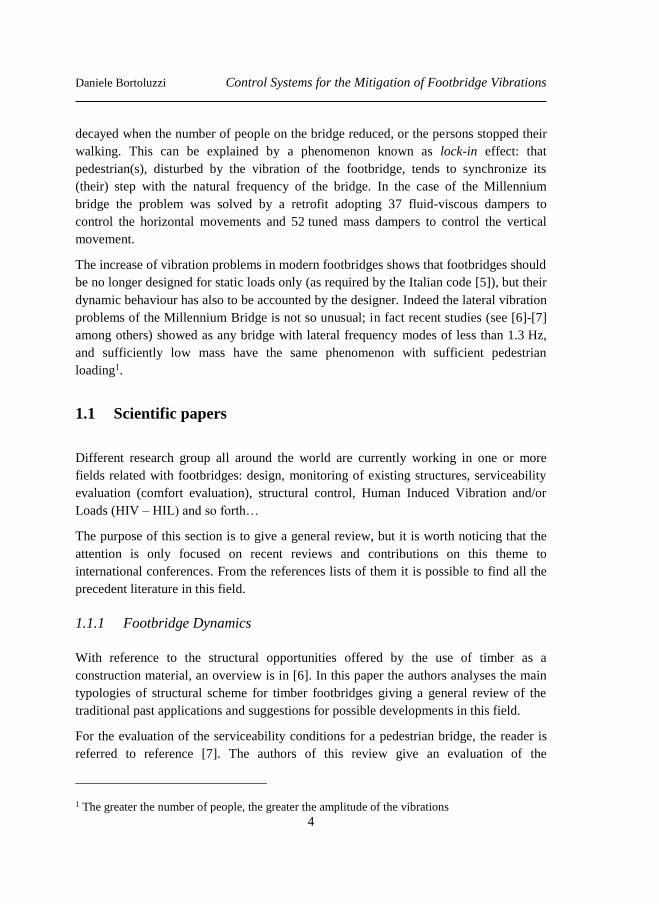
Based on a series of in situ experimental investigations, the author of [8] presents a new
vibration comfort criteria for footbridges (Figure 1.1.1).
Figure 1.1.1. Vibration comfort criteria for footbridges in case of human induced vibrations [8].
Moving to the monitoring of timber bridges, different papers have been published.
Indeed timber is very sensitive to the environmental changes, e.g. humidity, temperature
and so on (see [9] and [10] among others). In reference [11] an ah doc system of
devices for the monitoring of the footbridge is designed with the intent of evaluating
how the changes in the environment conditions can affect the modal response of the
structure. The duration of the data acquisition (1 year) and the number of sensors
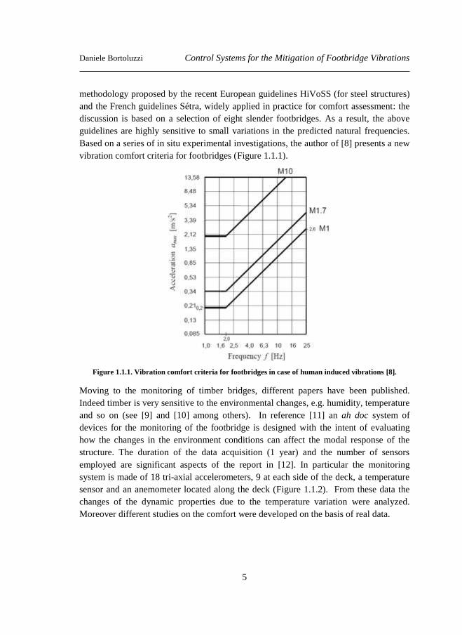
employed are significant aspects of the report in [12]. In particular the monitoring
system is made of 18 tri-axial accelerometers, 9 at each side of the deck, a temperature
sensor and an anemometer located along the deck (Figure 1.1.2). From these data the
changes of the dynamic properties due to the temperature variation were analyzed.
Moreover different studies on the comfort were developed on the basis of real data.
Daniele Bortoluzzi Control Systems for the Mitigation of Footbridge Vibrations
6
Figure 1.1.2. Monitoring system of the Pedro Gómez Bosque footbridge [12].
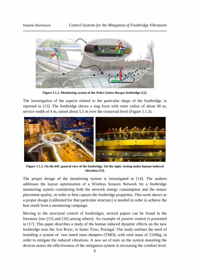
The investigation of the aspects related to the particular shape of the footbridge, is
reported in [13]. The footbridge shows a ring form with outer radius of about 40 m,
service width of 4 m, raised about 5,5 m over the crossroad level (Figure 1.1.3).
Figure 1.1.3. On the left: general view of the footbridge. On the right: testing under human induced
vibration [13].
The proper design of the monitoring system is investigated in [14]. The authors
addresses the layout optimization of a Wireless Sensors Network for a footbridge
monitoring system considering both the network energy consumption and the sensor
placement quality, in order to best capture the footbridge properties. This work shows as
a proper design (calibrated for that particular structure) is needed in order to achieve the
best result from a monitoring campaign.
Moving to the structural control of footbridges, several papers can be found in the
literature (see [15] and [16] among others). An example of passive control is presented
in [17]. This paper describes a study of the human induced dynamic effects on the new
footbridge over the Ave River, in Santo Tirso, Portugal. The study outlines the need of
installing a system of two tuned mass dampers (TMD), with total mass of 2100kg, in
order to mitigate the induced vibrations. A new set of tests on the system mounting the
devices assess the effectiveness of the mitigation system in increasing the comfort level.
Daniele Bortoluzzi Control Systems for the Mitigation of Footbridge Vibrations
7
This experience pointed out as the role of the damping is essential to mitigate the
vibration; in particular shows as the measured damping ratio is usually below the one
theoretically estimated. Thus, it is important to be very carefully in the estimation of the
damping. In [18] the authors implemented five MR-TMD control devices at the middle
span of the footbridge to be controlled under wind pressure. In particular a semi-active
strategy is adopted. The controllable Coulomb force is adjusted in a manner that its
value does not exceed the nominal maximum force of the MR damper but it is higher
than the nominal minimum force of the MR damper. The results show that the semi-
active control have a better control, in terms of acceleration performance, compared
with the classical passive control solution.
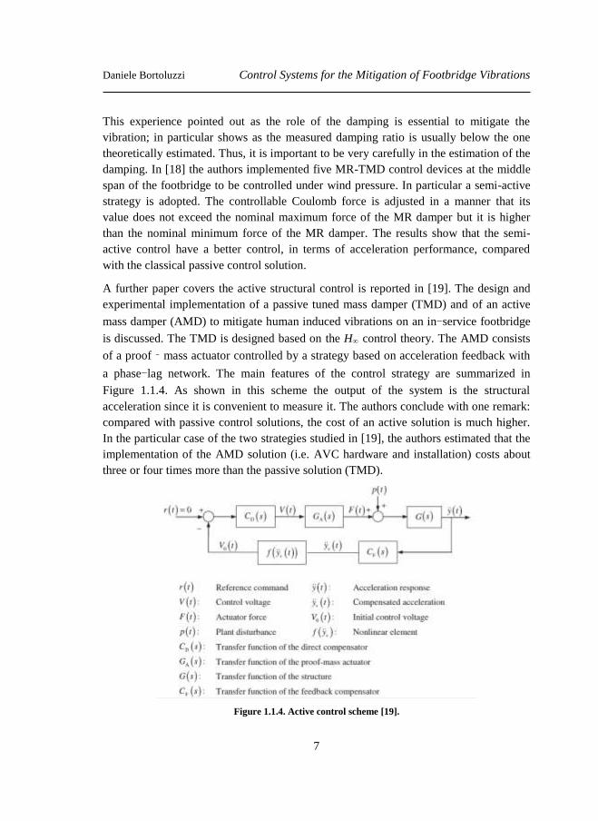
A further paper covers the active structural control is reported in [19]. The design and
experimental implementation of a passive tuned mass damper (TMD) and of an active
mass damper (AMD) to mitigate human induced vibrations on an in-service footbridge
is discussed. The TMD is designed based on the H∞ control theory. The AMD consists
of a proof‐mass actuator controlled by a strategy based on acceleration feedback with
a phase-lag network. The main features of the control strategy are summarized in
Figure 1.1.4. As shown in this scheme the output of the system is the structural
acceleration since it is convenient to measure it. The authors conclude with one remark:
compared with passive control solutions, the cost of an active solution is much higher.
In the particular case of the two strategies studied in [19], the authors estimated that the
implementation of the AMD solution (i.e. AVC hardware and installation) costs about
three or four times more than the passive solution (TMD).
Figure 1.1.4. Active control scheme [19].
Daniele Bortoluzzi Control Systems for the Mitigation of Footbridge Vibrations
8
1.1.2 Human Induced Vibration (HIV)
Consider now the topic of the Human Induced Vibration (HIV) [20]. The paper [21]
deals with the possibility of introducing simplified procedures to evaluate the maximum
dynamic response of footbridges due to a realistic loading scenario. Thus, a new non-
dimensional approach is introduced to identify the essential non-dimensional parameters
governing the dynamic behaviour under different loadings. Finally two simplified
procedures based on the definition of two coefficients, the Equivalent Amplification
Factor (EAF) and the Equivalent Synchronization Factor (ESF), are proposed with the
aim of assessing the vibration serviceability of a footbridge without the need of
numerical analyses. The coefficient EAF is defined as the ratio between the maximum
dynamic response to a realistic loading scenario and the maximum dynamic response to
a single resonant pedestrian, while ESF is the ratio between the maximum dynamic
response to a realistic loading scenario and the maximum dynamic response to
uniformly-distributed resonant pedestrian loadings. Moreover in [22], the human
walking is modelled using the random nature of the dynamic load due to pedestrians
walk. The probabilistic approach allows the designer to account for the variation of the
human walking force, due to the variation of the pedestrian weight, the step frequency,
the step length and the dynamic load factors (DLF), and so forth…, on the dynamic
response of the footbridges.
1.2 Recommendations and prescriptions
Timber footbridges with long span, and more generally all slender bridges, are sensitive
to vibrations, thus dynamic considerations have to be taken into account during the
design [12].
These sources of vibrations can be due to pedestrian traffic, and in particular by a crowd
of pedestrians walking along the deck in resonance with the bridge, or in extreme case
by rescue vehicles (e.g. ambulance) that may cross the bridge in emergency cases [22].
The general design rules regarding vibrations in timber footbridges reported in
Eurocode 5 ([23]), state that a bridge should be designed in a such a way that the loads
acting on the bridge do not result in uncomfortable vibrations for the pedestrian.
The basic question is: “how is possible to define a level of vibration comfortable or
uncomfortable?” As an example in Eurocode 0 ([24]) acceleration limits (Table 1.2.1)
regarding pedestrian induced vibrations are proposed, but no methods are given for the
evaluation of the dynamic behaviour. The code states that it is a designer’s
Daniele Bortoluzzi Control Systems for the Mitigation of Footbridge Vibrations
9
responsibility to make reasonable assumptions during the design stage and analysis to
guarantee that the proposed limits are fulfilled.
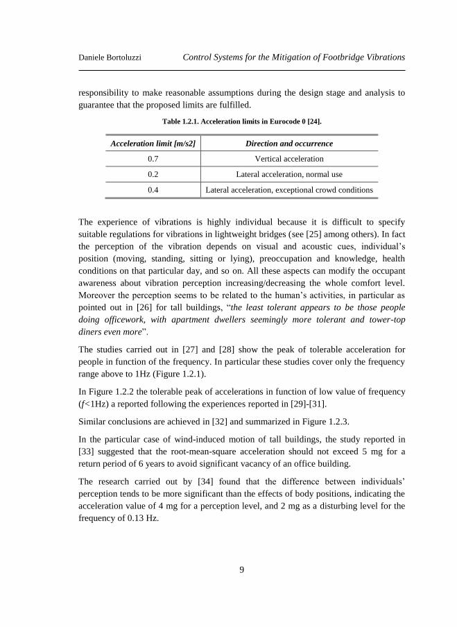
Table 1.2.1. Acceleration limits in Eurocode 0 [24].
Acceleration limit [m/s2] Direction and occurrence
0.7 Vertical acceleration
0.2 Lateral acceleration, normal use
0.4 Lateral acceleration, exceptional crowd conditions
The experience of vibrations is highly individual because it is difficult to specify
suitable regulations for vibrations in lightweight bridges (see [25] among others). In fact
the perception of the vibration depends on visual and acoustic cues, individual’s
position (moving, standing, sitting or lying), preoccupation and knowledge, health
conditions on that particular day, and so on. All these aspects can modify the occupant
awareness about vibration perception increasing/decreasing the whole comfort level.
Moreover the perception seems to be related to the human’s activities, in particular as
pointed out in [26] for tall buildings, “the least tolerant appears to be those people
doing officework, with apartment dwellers seemingly more tolerant and tower-top
diners even more”.
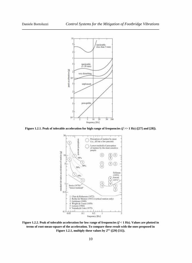
The studies carried out in [27] and [28] show the peak of tolerable acceleration for
people in function of the frequency. In particular these studies cover only the frequency
range above to 1Hz (Figure 1.2.1).
In Figure 1.2.2 the tolerable peak of accelerations in function of low value of frequency
(f<1Hz) a reported following the experiences reported in [29]-[31].
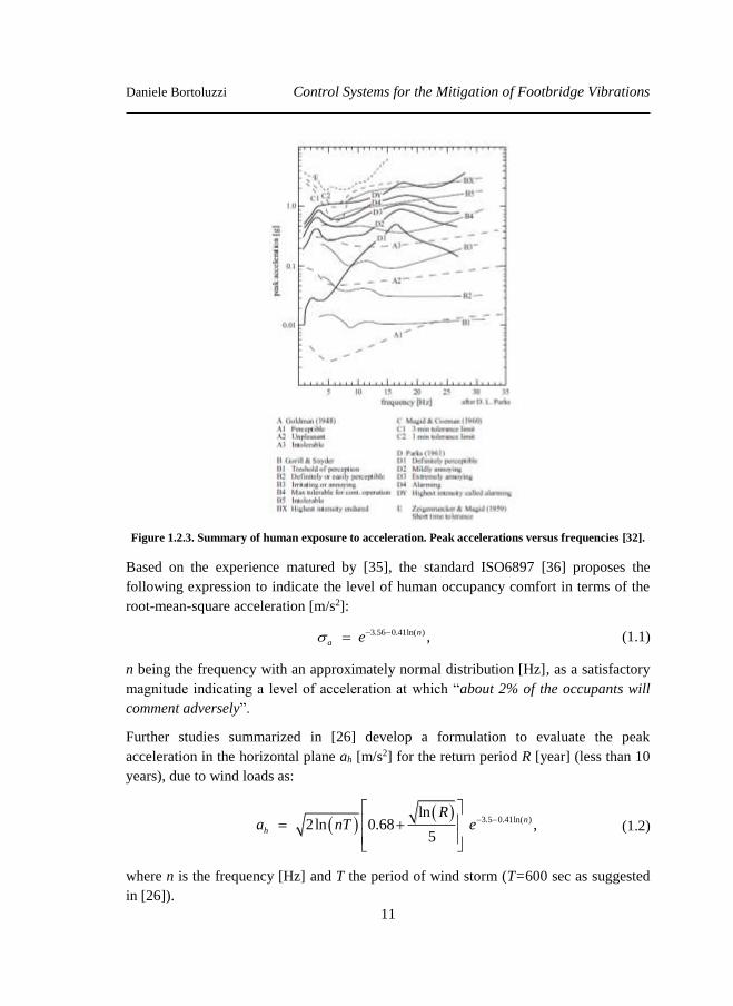
Similar conclusions are achieved in [32] and summarized in Figure 1.2.3.
In the particular case of wind-induced motion of tall buildings, the study reported in
[33] suggested that the root-mean-square acceleration should not exceed 5 mg for a
return period of 6 years to avoid significant vacancy of an office building.
The research carried out by [34] found that the difference between individuals’
perception tends to be more significant than the effects of body positions, indicating the
acceleration value of 4 mg for a perception level, and 2 mg as a disturbing level for the
frequency of 0.13 Hz.
Daniele Bortoluzzi Control Systems for the Mitigation of Footbridge Vibrations
10
Figure 1.2.1. Peak of tolerable acceleration for high range of frequencies (f >> 1 Hz) ([27] and [28]).
Figure 1.2.2. Peak of tolerable acceleration for low range of frequencies (f < 1 Hz). Values are plotted in
terms of root-mean-square of the acceleration. To compare these result with the ones proposed in
Figure 1.2.1, multiply these values by 20.5 ([29]-[31]).
Daniele Bortoluzzi Control Systems for the Mitigation of Footbridge Vibrations
11
Figure 1.2.3. Summary of human exposure to acceleration. Peak accelerations versus frequencies [32].
Based on the experience matured by [35], the standard ISO6897 [36] proposes the
following expression to indicate the level of human occupancy comfort in terms of the
root-mean-square acceleration [m/s2]:
3.56 0.41ln( ) , n
a e (1.1)
n being the frequency with an approximately normal distribution [Hz], as a satisfactory
magnitude indicating a level of acceleration at which “about 2% of the occupants will
comment adversely”.
Further studies summarized in [26] develop a formulation to evaluate the peak
acceleration in the horizontal plane ah [m/s2] for the return period R [year] (less than 10
years), due to wind loads as:
3.5 0.41ln( )ln
2ln 0.68 ,5
n
h
Ra nT e
(1.2)
where n is the frequency [Hz] and T the period of wind storm (T=600 sec as suggested
in [26]).
Daniele Bortoluzzi Control Systems for the Mitigation of Footbridge Vibrations
12
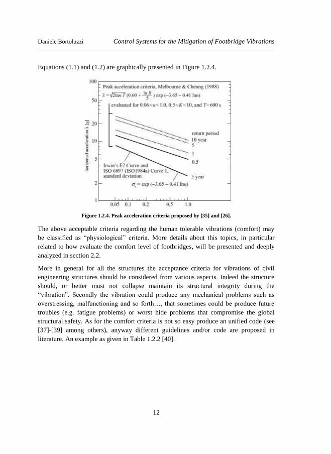
Equations (1.1) and (1.2) are graphically presented in Figure 1.2.4.
Figure 1.2.4. Peak acceleration criteria proposed by [35] and [26].
The above acceptable criteria regarding the human tolerable vibrations (comfort) may
be classified as “physiological” criteria. More details about this topics, in particular
related to how evaluate the comfort level of footbridges, will be presented and deeply
analyzed in section 2.2.
More in general for all the structures the acceptance criteria for vibrations of civil
engineering structures should be considered from various aspects. Indeed the structure
should, or better must not collapse maintain its structural integrity during the
“vibration”. Secondly the vibration could produce any mechanical problems such as
overstressing, malfunctioning and so forth…, that sometimes could be produce future
troubles (e.g. fatigue problems) or worst hide problems that compromise the global
structural safety. As for the comfort criteria is not so easy produce an unified code (see
[37]-[39] among others), anyway different guidelines and/or code are proposed in
literature. An example as given in Table 1.2.2 [40].
Daniele Bortoluzzi Control Systems for the Mitigation of Footbridge Vibrations
13
Table 1.2.2. German Standard DIN 4150 [40].
Acceleration limit [m/s2]
Peak velocity limits
Frequency range [Hz] Velocity [mm/s]
Industrial buildings f ≤ 10 20 20
Residential buildings 10 < f ≤ 50 15 + f/2 15 + f/2
Vulnerable buildings 50 < f ≤ 100 30 + f/5 30 + f/5
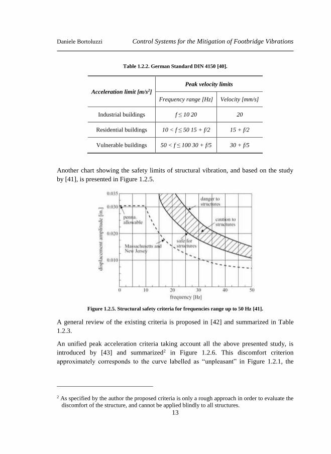
Another chart showing the safety limits of structural vibration, and based on the study
by [41], is presented in Figure 1.2.5.
Figure 1.2.5. Structural safety criteria for frequencies range up to 50 Hz [41].
A general review of the existing criteria is proposed in [42] and summarized in Table
1.2.3.
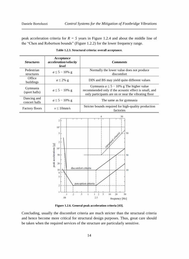
An unified peak acceleration criteria taking account all the above presented study, is
introduced by [43] and summarized2 in Figure 1.2.6. This discomfort criterion
approximately corresponds to the curve labelled as “unpleasant” in Figure 1.2.1, the
2 As specified by the author the proposed criteria is only a rough approach in order to evaluate the
discomfort of the structure, and cannot be applied blindly to all structures.
Daniele Bortoluzzi Control Systems for the Mitigation of Footbridge Vibrations
14
peak acceleration criteria for R = 5 years in Figure 1.2.4 and about the middle line of
the “Chen and Robertson bounds” (Figure 1.2.2) for the lower frequency range.
Table 1.2.3. Structural criteria: overall acceptance.
Structures
Acceptance
acceleration/velocity
level
Comments
Pedestrian
structures a ≤ 5 − 10% g
Normally the lower value does not produce
discomfort
Office
buildings a ≤ 2% g DIN and BS may yield quite different values
Gymnasia
(sport halls) a ≤ 5 − 10% g
Gymnasia a ≤ 5 − 10% g The higher value
recommended only if the acoustic effect is small, and
only participants are on or near the vibrating floor
Dancing and
concert halls a ≤ 5 − 10% g The same as for gymnasia
Factory floors v ≤ 10mm/s Stricter bounds required for high-quality production
factories
Figure 1.2.6. General peak acceleration criteria [43].
Concluding, usually the discomfort criteria are much stricter than the structural criteria
and hence become more critical for structural design purposes. Thus, great care should
be taken when the required services of the structure are particularly sensitive.
Daniele Bortoluzzi Control Systems for the Mitigation of Footbridge Vibrations
15
1.3 References
[1] Giacosa L.M.; A. De Stefano, 2007. Long-Term Structural Health Monitoring
of the 2006 Torino's Olympic Pedestrian Cabled-Stayed Bridge. In: SMSST'07,
Chonquing, Naijing - Cina, 19-27 Maggio 2007.
[2] Bursi, O. S., Ussia, A., Kumar, A., 2013. Structural health monitoring of a
complex cable-stayed footbridge and reliability assessment. On the Proceeding
of the 11th International Conference on Structural Safety & Reliability -
ICOSSAR 2013, New York, USA, June 16-20, 2013.
[3] Bonelli A, Bursi, O. S. , Ceravolo R., Santini S., Tondini N., Zasso A., 2010.
Dynamic Identification and Structural Health Monitoring of a Twin Deck
Curved Cable-Stayed Footbridge: The “Ponte Del Mare” of Pescara in Italy".
On the Proceeding of the Fifth European Workshop on Structural Health
Monitoring, Sorrento, Naples, Italy, 29 June - 02 July, 2010.
[4] P. Dallard et al. 2001. The London Millennium Footbridge. The Structural
Engineer Volume 79/No 22.
[5] Norme tecniche per le costruzioni - D.M. 14 Gennaio 2008 (NTC2008) [In
Italian].
[6] Zobel H., Alkhafaji T., 2011. Contemporary Structural Solutions Of Timber
Pedestrian Bridges On the Proceeding of the 4th International Conference
Footbridge - Wrocław (Poland) on July 6th – 8th, 2011.
[7] K. Van Nimmen, G. Lombaert, G. De Roeck, P. Van den Broeck, 2014.
Vibration serviceability of footbridges: Evaluation of the current codes of
practice. Engineering Structures 59, pp. 448–461.
[8] M. Pańtak, 2012.Elaboration of the vibration comfort criteria for footbridges
during vibrations induced by pedestrians. Bridge Maintenance, Safety,
Management, Resilience and Sustainability – Biondini & Frangopol (Eds) -
Taylor & Francis Group, London, ISBN 978-0-415-62124-3.
[9] Bortoluzzi D., Casciati F., Casciati S., Faravelli L., Chen Z., 2013. Reporting
the results of two experimental campaigns on a pedestrian timber bridge - 9th
International Workshop on Structural Health Monitoring 2013 – IWSHM -
Stanford University, Stanford, CA – USA, September 10-2, 2013.
[10] Bortoluzzi D., Casciati F., Casciati S., Faravelli L, 2013. Comparison of
accelerometric response records on a timber footbridge. On the Proceeding of
Daniele Bortoluzzi Control Systems for the Mitigation of Footbridge Vibrations
16
2nd International Conference on Timber Bridges 2013 – ICTB2013, Las
Vegas, Nevada USA, September-October, 2013.
[11] Iván M. Díaz, José M. Soria, Norberto Ibán, Mariano Cacho Pérez, Jaime
García-Palacios, 2014. Vibration Monitoring of a Steel-plated Stress-ribbon
Footbridge: Effects of Environmental and Operational Factors on Modal
Properties. On the Proceeding of the 6th World Conference on Structural
Control and Monitoring - 6WCSCM, Barcellona, Spain, 15-17 July, 2014.
[12] Antolín Lorenzana et al., 2014. One year of the structural health monitoring of
Pedro Gómez Bosque footbridge. On the Proceeding of the 6th World
Conference on Structural Control and Monitoring - 6WCSCM, Barcellona,
Spain, 15-17 July, 2014.
[13] Siwowski T., Janas L., 2014. Numerical and experimental assessment of the
dynamic behaviour of a circular footbridge. On the Proceeding of the 9th
International Conference on Structural Dynamics, EURODYN 2014 Porto,
Portugal, 30 June - 2 July 2014.
[14] K. Jalsan, K. Flouri & G. Feltrin, 2012. Bi-Objective Layout Optimization of a
Wireless Sensor Network for Footbridge Monitoring. Bridge Maintenance,
Safety, Management, Resilience and Sustainability – Biondini & Frangopol
(Eds) - Taylor & Francis Group, London, ISBN 978-0-415-62124-3.
[15] Bortoluzzi, D., Casciati, S., Elia, L., Faravelli, L. 2013. Semi-Active Control
for the Mitigation of the Vibration on a Footbridge. On the Proceeding of XXI
Congresso dell’Associazione Italiana di Meccanica Teorica ed Applicata –
AIMETA2013 – Torino , Italy, September, 17-20, 2013.
[16] Bortoluzzi, D., Casciati, F., Faravelli, L. 2014. Vibration mitigation in a
“cable-stayed-like” timber footbridge. On the Proceeding of the 6th World
Conference on Structural Control and Monitoring - 6WCSCM, Barcellona,
Spain, 15-17 July, 2014.
[17] Rodrigo Falcão Moreira, Elsa Caetano, Álvaro Cunha, 2014. Vibration control
and monitoring on the new footbridge over the Ave River in Santo Tirso,
Portugal. On the Proceeding of the 9th International Conference on Structural
Dynamics, EURODYN 2014 Porto, Portugal, 30 June - 2 July 2014.
[18] J. Liu, L. Jiang, S.J. Li, Q. Zhou, and R.C. Zhang, 2014. Smart control for
responses of footbridge induced by wind pressure due to high speed train using
MR-TMD system. On the Proceeding of the 6th World Conference on
Daniele Bortoluzzi Control Systems for the Mitigation of Footbridge Vibrations
17
Structural Control and Monitoring - 6WCSCM, Barcellona, Spain, 15-17 July,
2014.
[19] Carlos M. Casado et al., 2013.Implementation of passive and active vibration
control on an in-service footbridge. Journal of Structural Control And Health
Monitoring; 20, pp. 70–87.
[20] Casciati S., Faravelli L., Bortoluzzi D., 2013. Human Induced Vibrations In A
Pedestrian Timber Bridge. On the Proceeding of the 4th International
Conference on Computational Methods in Structural Dynamics & Earthquake
Engineering - COMPDYN2013, Kos Island (GR), 12-14 Jun 2013.
[21] Piccardo G., Tubino F., 2009. Simplified procedures for vibration
serviceability analysis of footbridges subjected to realistic walking loads.
Journal of Computers and Structures 87, pp. 890–903.
[22] José Guilherme Santos da Silva, Jorge Maurício dos Santos de Souza, 2014.
Dynamic analysis of pedestrian footbridges based on probabilistic modelling.
On the Proceeding of the 9th International Conference on Structural Dynamics,
EURODYN 2014 Porto, Portugal, 30 June - 2 July 2014.
[23] Eurocode 5 - EN 1995-2:2004. Design of timber structures - Part2: Bridges, 1st
edition.
[24] Eurocode 0 - EN 1990. Basis of structural design, 1st edition.
[25] Kliger R., Svensson T. , J. and I. Svensson, 2013. Vibration response of long
cable-stayed timber footbridge – case study. On the Proceeding of 2nd
International Conference on Timber Bridges 2013 – ICTB2013, Las Vegas,
Nevada USA, September-October, 2013.
[26] Melbourne W. and Cheung J., 1988. Designing for serviceable accelerations in
tall buildings. Proceedings of the 4th International Conference on Tall
Buildings, pp. 148–155, Hong Kong and Shanghai.
[27] Harris C., 1976. Shock and Vibration Handbook, 2nd edn. McGraw-Hill.
[28] Wiss F. and Parmelee R., 1974. Human perception of transient vibrations
Proceedings of the American Society of Civil Engineers, 100 (ST4), 773–787.
[29] Chen P. and Robertson L., 1973. Human perception thresholds of horizontal
motion. Proceedings of the American Society of Civil Engineers, 98, 1681–
1695.
Daniele Bortoluzzi Control Systems for the Mitigation of Footbridge Vibrations
18
[30] Irwin P., 1979. Human response to dynamic motion of structures. The
Structural Engineer 9(56A), pp. 237–244.
[31] Melbourne W., 1998. Comfort criteria for wind-induced motion in structures.
Structural Engineering International 8(1), pp. 40–44.
[32] Chang F (1973) Human response to motions in tall buildings. Proceedings of
the American Society of Civil Engineers, 98, pp. 1259–1272.
[33] Hansen R., Reed J. and Vannarcke E., 1974. Human response to wind-induced
motion on buildings. Proceedings of the American Society of Civil Engineers,
99, 1589–1605.
[34] Khan F. and Parmelee R., 1971. Service criteria for tall buildings for wind
loading. Proceedings of the 3rd International Conference Wind Effects on
Buildings and Structures, pp. 401–408, Tokyo.
[35] Irwin P., 1986. Motion in tall buildings. Proceedings of the Conference on Tall
Bridges and Urban Habitat, pp. 759–778, Chicago.
[36] ISO 6897, 1984. Guidelines for the Evaluation of the Response Occupants of
Fixed Structures, Especially Buildings and Off-shore Structures, to Low
Frequency Horizontal Motion (0.063 to 1 Hz). ISO, International Standards
Organization.
[37] ISO/DIS 4866, 1984. Mechanical Vibrations and Shock Measurement and
Evaluation of Vibration Effects on Buildings. International Standards
Organization.
[38] ISO 2373, 1987. Mechanical vibration of certain rotating electrical machinery
with shaft heights between 80 and 400 mm - Measurement and evaluation of
the vibration severity. International Standards Organization.
[39] ISO 10816, 1995. Mechanical vibration -- Evaluation of machine vibration by
measurements on non-rotating parts. International Standards Organization.
[40] German Standard DIN 4150 [41].
[41] Leet L., 1960. Vibrations from Blasting Rocks. Harvard University Press.
[42] Bachmann H. and Ammann W., 1987. Vibrations in structures – induced by
man and machines. In Structural Engineering Documents, 3rd edn, 1ABSE,
Zurich (Switzerland).
[43] Wenzel H., 2009. Health Monitoring of Bridges. John Wiley & Sons Ltd, The
Atrium, Southern Gate, Chichester, West Sussex PO19 8SQ, England.
Daniele Bortoluzzi Control Systems for the Mitigation of Footbridge Vibrations
19
Chapter 2 Design requirements and performance
satisfaction
As already observed in the previous chapter, one of the main problems when one works
on footbridges, is not the safety aspect, but rather the limitation of the vibration in order
to achieve a good result in term of comfort for the user.
This means that footbridges should be no longer designed for static loads only, but also
accounting for the dynamic behaviour during the design stage, without forgetting the
rule of thumb: “the more slender structures become, the more attention must be paid to
vibration phenomena”.
One of the main and simplest way if one wants to take into control the vibration of a
given footbridge is that one has to keep the natural frequency within a suitable range as
will be better analyzed and discussed in section 2.2 (see [1]-[2] among others). To fulfil
such a requirements, one could be forced to a special footbridge design; in fact very
slender and/or lightweight structures, suspension bridges and so forth… could be unable
to satisfy these requirements. Not only natural frequencies but also mass, damping, deck
loading (pedestrian loads) determines the dynamic behaviour of the footbridge.
These bridges are usually characterized by the lowest value of the natural frequencies
very close to the external excitations like that of the pedestrian loads; thus the risk of
resonance is quite great. Vibrations of footbridges may occur in vertical and horizontal
directions. Even the torsion of the bridge deck is sometimes excited.
Vibrations of footbridges may lead to serviceability problems, affecting the comfort of
the crossing pedestrians. Collapse or even damage due to human induced dynamic
forces are quite unlikely to occur. For these kinds of structures, the pedestrian induced
load3 is probably the main source of vibration of footbridges, together with the wind
loads.
3 Pedestrian loading is by nature unsteady, transient and waddling in a small range of excitation
frequency.
Daniele Bortoluzzi Control Systems for the Mitigation of Footbridge Vibrations
20
Another dynamic loading on footbridges is intentional excitation by people that are
jumping on the spot, bouncing, swaying body horizontally, shaking stay cables etc… In
that case, the comfort is certainly not fulfilled but the structure should preserves its
integrity under these extreme loads must be considered.
Summarizing, in general the assessment of human-induced vibrations needs to be
considered by the designer during the design to evaluate that:
1) vibrations due to pedestrian traffic are acceptable for the users (comfort
aspects),
2) the footbridge does not collapse when subjected to intentional excitation
(safety aspects due to extreme loads).
Once proved that the dynamic behaviour of the bridge due to expected loads is
evaluated and fulfilled the required comfort, the footbridge can be designed and
constructed. If the vibration behaviour does not satisfy some comfort criteria, changes in
the design or damping devices should be considered.
Concluding, a well done footbridge design should consider all these factors in order to
match together structural (both from static and dynamic point of view) and architectural
aspects with the comfort requirements.
2.1 Dynamics of the footbridges design and structural health
monitoring
The purpose of this section is to recall the main features and concepts within the
dynamic of the structures (see [3]-[5] among others) and the structural health
monitoring (see [6]-[8] among others).
2.1.1 Governing relations
Fort the general formulation of the dynamic problem the reader will be referred to [9]-
[14] among others.
Most of the structural dynamic properties can be highlighted studying the so called
simple oscillator. The simple oscillator (discrete system) consists of mass m, connected
to a support by a linear spring of stiffness k and a linear damper of viscosity c, on which
is acting an external force F(t). It is supposed that the device moves only in one
direction; therefore one has only one degree of freedom (1-DOF) defined by the
position x(t) of its mass (Figure 2.1.1).
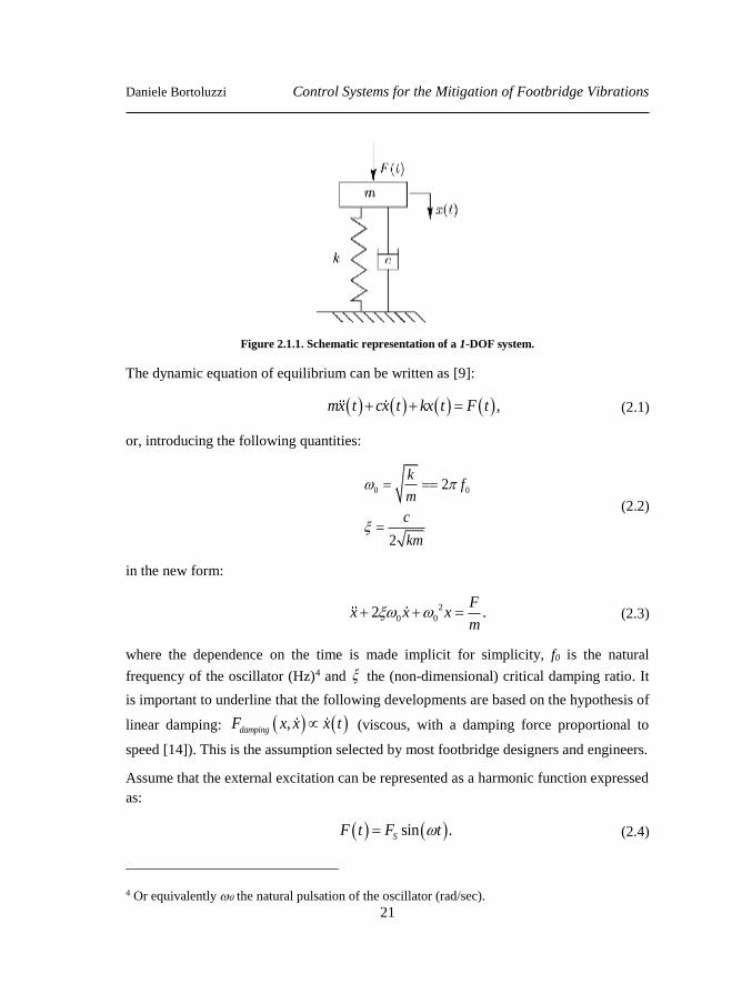
Daniele Bortoluzzi Control Systems for the Mitigation of Footbridge Vibrations
21
Figure 2.1.1. Schematic representation of a 1-DOF system.
The dynamic equation of equilibrium can be written as [9]:
,mx t cx t kx t F t (2.1)
or, introducing the following quantities:
0 02
2
kf
m
c
km
(2.2)
in the new form:
2
0 02 .F
x x xm
(2.3)
where the dependence on the time is made implicit for simplicity, f0 is the natural
frequency of the oscillator (Hz)4 and the (non-dimensional) critical damping ratio. It
is important to underline that the following developments are based on the hypothesis of
linear damping: ,dampingF x x x t (viscous, with a damping force proportional to
speed [14]). This is the assumption selected by most footbridge designers and engineers.
Assume that the external excitation can be represented as a harmonic function expressed
as:
sin .SF t F t (2.4)
4 Or equivalently the natural pulsation of the oscillator (rad/sec).
Daniele Bortoluzzi Control Systems for the Mitigation of Footbridge Vibrations
22
Then it is possible to evaluate the “static” response of the oscillator under the action of
an equivalent force of amplitude equal to FS; that is:
0
0
2
0
.static
FF mxk
(2.5)
From this it is possible to determine the maximum dynamic response of the system by
simply multiplying the static response by the dynamic amplification parameter A(Ω):
,max staticx x A (2.6)
where 0 is the relative pulsation (or reduced pulsation), and the dynamic
amplification parameter can be represented as a function of the relative pulsation and
the critical damping ratio:
22 2 2
1.
1 4
A
(2.7)
These parameter may be represented by a set of curves parameterized by as reported
in Figure 2.1.2.
These curves show a peak for the value of 21 2R characterising the resonance5
and therefore corresponding to the resonance frequency:
2
02 1 2 .R R Rf (2.8)
It is worth underlining that the resonance phenomena for a damped structure occurs
when the frequency of the external excitation equals the resonance frequency; that is
R .
Since the structural damping for the usual civil structures is weak ([9] and [13]), i.e.
1 , one may consider that resonance occurs when:
0
11 1 .
2R R RA
(2.9)
5 Resonance is the tendency of a system to oscillate with greater amplitude at some frequencies
than at others. At these frequencies, even small periodic driving forces can produce large
amplitude oscillations.

Daniele Bortoluzzi Control Systems for the Mitigation of Footbridge Vibrations
23
Figure 2.1.2. Dynamic parameter trend for specific value of the critical damping.
The above properties, even if introduced for a 1-DOF, show that designing the
structures only taking into account the maximum intensity (FS) of the acting load can
result to be unsatisfactory. In fact the resonance phenomenon can generate higher
displacements/ stresses even if the intensity of the loads is lower. Thus, for example, the
force 1 1sinSF t F t can generate displacements or stresses much lower than a load
with an amplitude 10 times weaker, 2 210 sinSF t F t , only because F2(t) has a
frequency much closer to the resonance frequency of the structure. Moreover the
resonance amplification is directly related to damping.
The most common sources of damping are:
1) the internal damping linked with the material itself; its value is mainly linked
to the temperature and the frequency of excitation;
2) the damping by friction (Coulomb) , ( )dampingF x x sign x : it is mainly
linked to the construction joints between different elements.
Just to illustrate how the damping acts on the response of the oscillator, consider the so
called free vibration: assume that the external force is equal to zero over the time
(F(t)=0). Thus, re-writing equation (2.3) one achieves:
2
0 02 0.x x x (2.10)
The generic solution of the above differential equation can be expressed as:
0 ,
rtx t X e (2.11)
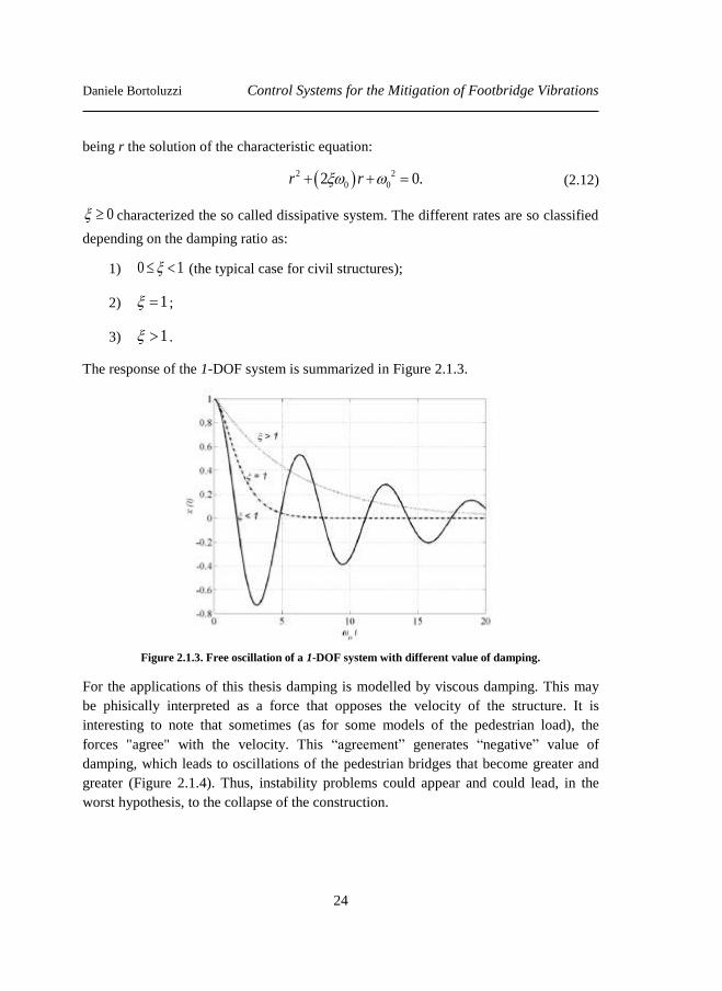
Daniele Bortoluzzi Control Systems for the Mitigation of Footbridge Vibrations
24
being r the solution of the characteristic equation:
2 2
0 02 0.r r (2.12)
0 characterized the so called dissipative system. The different rates are so classified
depending on the damping ratio as:
1) 0 1 (the typical case for civil structures);
2) 1 ;
3) 1 .
The response of the 1-DOF system is summarized in Figure 2.1.3.
Figure 2.1.3. Free oscillation of a 1-DOF system with different value of damping.
For the applications of this thesis damping is modelled by viscous damping. This may
be phisically interpreted as a force that opposes the velocity of the structure. It is
interesting to note that sometimes (as for some models of the pedestrian load), the
forces "agree" with the velocity. This “agreement” generates “negative” value of
damping, which leads to oscillations of the pedestrian bridges that become greater and
greater (Figure 2.1.4). Thus, instability problems could appear and could lead, in the
worst hypothesis, to the collapse of the construction.
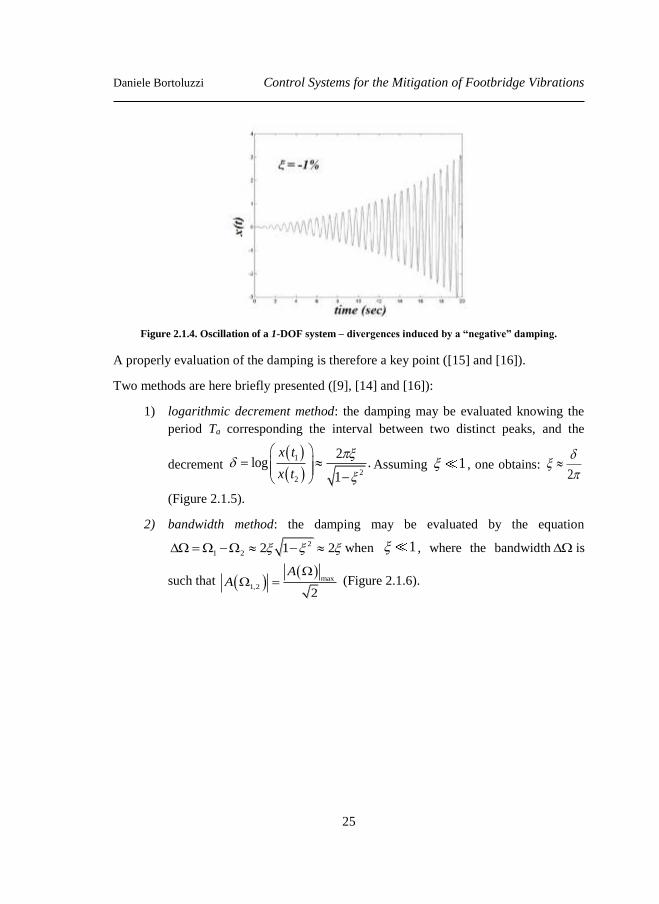
Daniele Bortoluzzi Control Systems for the Mitigation of Footbridge Vibrations
25
Figure 2.1.4. Oscillation of a 1-DOF system – divergences induced by a “negative” damping.
A properly evaluation of the damping is therefore a key point ([15] and [16]).
Two methods are here briefly presented ([9], [14] and [16]):
1) logarithmic decrement method: the damping may be evaluated knowing the
period Ta corresponding the interval between two distinct peaks, and the
decrement
1
22
2log .
1
x t
x t
Assuming 1 , one obtains:
2
(Figure 2.1.5).
2) bandwidth method: the damping may be evaluated by the equation
2
1 2 2 1 2 when 1 , where the bandwidth is
such that
max
1,22
AA
(Figure 2.1.6).
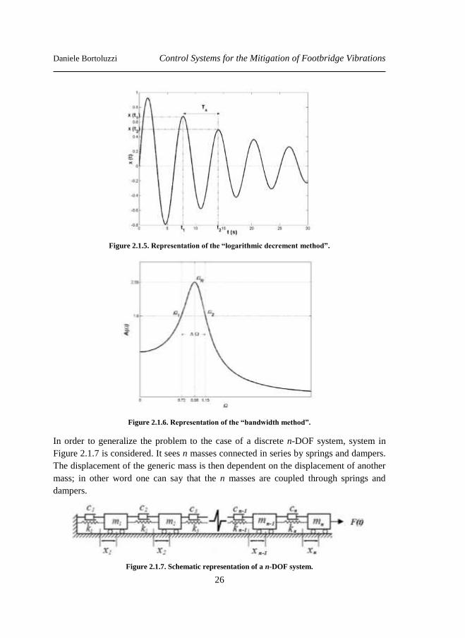
Daniele Bortoluzzi Control Systems for the Mitigation of Footbridge Vibrations
26
Figure 2.1.5. Representation of the “logarithmic decrement method”.
Figure 2.1.6. Representation of the “bandwidth method”.
In order to generalize the problem to the case of a discrete n-DOF system, system in
Figure 2.1.7 is considered. It sees n masses connected in series by springs and dampers.
The displacement of the generic mass is then dependent on the displacement of another
mass; in other word one can say that the n masses are coupled through springs and
dampers.
Figure 2.1.7. Schematic representation of a n-DOF system.
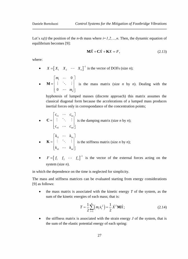
Daniele Bortoluzzi Control Systems for the Mitigation of Footbridge Vibrations
27
Let’s xi(t) the position of the n-th mass where i=1,2,…,n. Then, the dynamic equation of
equilibrium becomes [9]:
,X X X F M C K (2.13)
where:
1
1 2 nX X X X
is the vector of DOFs (size n);
1 0
0 n
m
m
M is the mass matrix (size n by n). Dealing with the
hyphotesis of lumped masses (discrete approach) this matrix assumes the
classical diagonal form because the accelerations of a lumped mass produces
inertial forces only in correspondance of the concentration points;
11 1
1
n
n nn
c c
c c
C is the damping matrix (size n by n);
11 1
1
n
n nn
k k
k k
K is the stiffness matrix (size n by n);
1
1 2 nF f f f
is the vector of the external forces acting on the
system (size n).
in which the dependence on the time is neglected for simplicity.
The mass and stiffness matrices can be evaluated starting from energy considerations
[9] as follows:
the mass matrix is associated with the kinetic energy T of the system, as the
sum of the kinetic energies of each mass; that is:
2
1
1
1 1;
2 2
nT
i
i
T m x X X
M (2.14)
the stiffness matrix is associated with the strain energy J of the system, that is
the sum of the elastic potential energy of each spring:
Daniele Bortoluzzi Control Systems for the Mitigation of Footbridge Vibrations
28
22 2
11 1 12 2 1 1
1 1;
2 2
T
nn nJ k x k x x k x X X
K (2.15)
These two matrices are both symmetric, moreover the mass matrix is positive definite
(because the kinetic energy is always positive by definition), while the stiffness matrix
is positive semi-definite because of definition.
For n-DOF systems it is useful to introduce the modal superposition approach [14].
Consider the free movement case, thus the equation of motion (2.13) can be re-written
as:
0,X X M K (2.16)
where the generic vector solution may be represented as:
0 e ,rtX (2.17)
in which 0 is a vector of constant to be determinate, of size n. Substituting (2.17) into
(2.16) one reach:
2
0 0.r K+ M (2.18)
The above equation admits advantageous solutions only if the determinant of the system
is equal to zero; that is only if:
2det 0.r K+ M (2.19)
For a classical n-DOF system the above system has 2n solutions: , 1,2, ,ki k n
where k represents the k-th natural pulsation of the system. With each index k, there is
an associated vector called modal vectors of the system k such that the response of the
whole system can be re-written as:
1
e e .k k
ni t i t
k k k
k
X t
(2.20)
The components of the vector k are linked, thus usually these modal vectors are
defined after normalization. The most frequent choices are here summarized:
one of the components is made equal to 1.
each mode is unitary; i.e. 1;i
Daniele Bortoluzzi Control Systems for the Mitigation of Footbridge Vibrations
29
satisfy the requirement: 1.T
i i M
Summarizing, the natural pulsations i are the square roots of the natural positive
values of the matrix 1K
M evaluable solving the equation 2det 0.i K M The
natural forms of a discrete system are the natural vectors i associated with it. The
couple ,i i is called a natural vibration mode where i=1,2,…,n. In other words for a
linear system a mode is one particular solution of the free non-damped vibration, in
which all the DOFs components are synchronous6:
0
0mode0e .
i tX t
(2.21)
The above natural vibration modes are orthogonal in relation to the mass matrix and in
relation to the stiffness matrix [9]; that is:
, ,
T
i j i ij
T
i j i ij
mi j
k
M
K (2.22)
in which ij is the classical Kronecker symbol, while mi and ki represent, respectively,
the so called generalised mass and stiffness associated to i-th mode. Their values will
depend on the normalization used to define the natural vectors as described above.
To the case of non-damped forced vibration, the dynamic equilibium (2.13) become as:
.X X F M K (2.23)
To solve directly the above equation needs to evaluate the inverse of the mass matrix
that could be costly, from the calculation point of view, if the number of DOFs is high.
Thus, it is standard practice to apply the modal superposition approach. This way is
quite useful because it is able to unlinks the equations of motion that compose the
general equations, significantly reducing the calculation operations. The principle
behind this approach is to introduce a reference change re-writing the equation of
motion in the new base system obtained by a linear combination of the natural vectors i
the so called modal base. Thus, the response X(t) of the system represented by equations
(2.23) may be expressed as:
1
,n
i i
i
X t q t q t
(2.24)
6 That is they reach their maxima and their minima at the same time.
Daniele Bortoluzzi Control Systems for the Mitigation of Footbridge Vibrations
30
in which:
1 2 n is a matrix (size n by n) where each columns contain the
natural vector i ;
q t is the vector the modal variables, the new variables obtained re-writing
the problem in the new reference system.
Having in mind the orthogonality of the modes, see (2.22), and the generic solution in
(2.24), pre-multiplying equation (2.23) by T one obtains:
T T T Tq t q t F t q t q t F t M (2.25)
or in extended form:
0 0 0 0
0 0 0 0 .
0 0 0 0
T
i im q t k q t F t
(2.26)
where , are respectively the diagonalized mass and stiffness matrices. This allows
one to get a system of unlinked differential equations as:
2 ,i iq t q t p t (2.27)
where the vector T
i
i
Fp t
m
contain the component per unit of generalized mass of
the force vector F(t), and it is called the modal contribution factors of the applied force
vector.
The possibility of writing the general problem expressed by equation (2.23) in
diagonalized form should be achieved in order to decrease the computational cost as
observed. The presence of damping matrix C makes the problem a little bit more
complicated. In fact, as far as the damping matrix C is a general matrix, it is not
possible to state that this matrix will also be diagonalized by the modal superposition
approach. However, there are some cases where this property does apply. The most
remarkable case when a matrix C is transformed into a diagonal matrix by the modal
approach is the one called “proportional damping”. In fact when the structure under
study is not to much dissipative and the natural frequencies are clearly separated, it can
be shown that is reasonable ([9] and [14]) to define the damping matrix as a linear
combination of the mass and stiffness matrices; that is:
Daniele Bortoluzzi Control Systems for the Mitigation of Footbridge Vibrations
31
1
1
1
, .N
j
j j
j
C= M M K (2.28)
Assuming in the above equation N=2 one achieves:
1 2 , C= M+ K (2.29)
the so called Rayleigh’s damping matrix, where 1 and 2 are two constant parameters
called Rayleigh’s coefficients, whose values define the entity of damping actions in the
system, that in the International System have the physical dimension of s-1 and s
respectively.
Since both the mass and stiffness matrices may be diagonalized applying the modal
approach (see equation (2.23)), is simple to observe as the damping matrix expressed by
will also be diagonalized by following the same approach; indeed:
1 2 1 2 .T T C M+ K Μ+ Κ (2.30)
Thus, the n equations of motion of the generic system described in (2.23) are decoupled.
Then one considers each single equation as represented by a 1-DOF system as follows7:
22 ,i i i iq t q t q t p t (2.31)
where 2
ii
i im
in which 1 2i i im k . In practice, each critical damping ratio i
must be experimentally recalibrated and/or evaluated. By the way it is usual to consider
that the value of the critical damping ratio does not depend on the mode under
consideration. This allows one to assume i , where the constant value is fixed
experimentally or by the regulations [36].
In conclusion the principle of modal superposition allows one to treat the generic n-
DOF system as the “sum” of n simple oscillators (Figure 2.1.8), once a new reference
frame has been introduced.
7 This formulation can be seen as a generalization of equation (2.27).
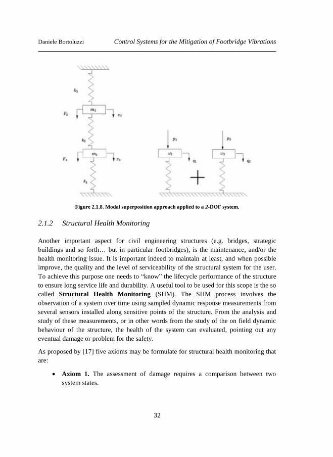
Daniele Bortoluzzi Control Systems for the Mitigation of Footbridge Vibrations
32
Figure 2.1.8. Modal superposition approach applied to a 2-DOF system.
2.1.2 Structural Health Monitoring
Another important aspect for civil engineering structures (e.g. bridges, strategic
buildings and so forth… but in particular footbridges), is the maintenance, and/or the
health monitoring issue. It is important indeed to maintain at least, and when possible
improve, the quality and the level of serviceability of the structural system for the user.
To achieve this purpose one needs to “know” the lifecycle performance of the structure
to ensure long service life and durability. A useful tool to be used for this scope is the so
called Structural Health Monitoring (SHM). The SHM process involves the
observation of a system over time using sampled dynamic response measurements from
several sensors installed along sensitive points of the structure. From the analysis and
study of these measurements, or in other words from the study of the on field dynamic
behaviour of the structure, the health of the system can evaluated, pointing out any
eventual damage or problem for the safety.
As proposed by [17] five axioms may be formulate for structural health monitoring that
are:
Axiom 1. The assessment of damage requires a comparison between two
system states.

Daniele Bortoluzzi Control Systems for the Mitigation of Footbridge Vibrations
33
Axiom 2. The identification of the existence and location of damage can be
done in an unsupervised learning mode, but the type of damage and the damage
severity can only be identified in a supervised learning mode.
Axiom 3. Without intelligent feature extraction, the more sensitive a
measurement is to damage, the more sensitive it is to changing operational and
environmental conditions.
Axiom 4. There is a trade-off between the sensitivity to damage of an
algorithm and its noise rejection capability.
Axiom 5. The size of damage that can be detected from changes in system
dynamics is inversely proportional to the frequency range of excitation.
In the civil engineering area SHM requires to take account for numerous non linearity
and not well known “boundary” condition of the problem, as in the case of soil structure
interaction. Thus, the SHM key of success is enclosed in the possibility to collect high
quality data combined with realistic identified models and deterioration laws [12]. The
final output of a SHM could be the reliability index, the safety level, a graphic symbol
or any other output depending on the owner [18]. An example of a SHM architecture
applied to a bridge case is reported in Figure 2.1.9. Another example can be found in
[19].
In the last years different approaches were proposed for health monitoring (see [20]-[24]
among others). It is important that the data collected during the experimental campaign
by accurately stored in order to, first of all, create a database for the structure, and apply
new future algorithms when available to compare the structural behaviour between the
“old” and “new” data analysis approach. By the way, it is important to note that to
achieve a whole computerized SHM system able to make decision about the structural
health monitoring by itself is far away.
It is clear now as SHM provides the opportunity to quantify the condition of the
structure and gives the guidelines for making decisions about the structure (Figure
2.1.10), since the dynamic characteristic contains information on the global structural
condition as well as on local phenomena [13].

Daniele Bortoluzzi Control Systems for the Mitigation of Footbridge Vibrations
34
Figure 2.1.9. SHM architecture applied to a bridge [12].
Figure 2.1.10. Example of proposed rehabilitation planning based on the Ultimate Limit Strength [13].
Three different mains topics could be taken into account when one wants to perform a
SHM:
1) responsibility;
2) economy;
3) curiosity.

Daniele Bortoluzzi Control Systems for the Mitigation of Footbridge Vibrations
35
From the above-mentioned motivations it is necessary to offer services on increasing
quality levels depending on the structure under study and so to the depths of
investigation that one wants to perform. Usually five level of investigation (Figure
2.1.11) are introduced within bridges field according to [12]:
Level 1 - Rating: this represents the basic/conventional assessment of the
structure starting with a visual field inspection that provides a subjective
impression of the condition of the structure.
Level 2 - Condition assessment: rough visual field inspection after which is
possible to decide whether the conventional approach is satisfactory or an
extended one is needed. Moreover this inspection will determine the type and
quantity of instrumentation that will be used on field.
Level 3 - Performance assessment: provides additional indicators for the
assessment and will demonstrate the performance of the structure. It requires
several synchronous devices to perform the monitoring.
Level 4 - Detail assessment and rating: establish an analytical model
representing the structure. The numerical model will be compared with the
result collected during the monitoring campaign(s).
Level 5 - Lifetime prediction: the last step regards the lifetime evaluation (see
Figure 2.1.12 as proposed in [25]). To achieve a serious lifetime prediction the
records available have to be long enough to cover, at least, three relevant
cycles for the structure (e.g. usually at least three years).
To achieve the above purpose, a selection of suitable data has to be made. In particular
one can have four different levels of monitoring,, that are:
1) spot monitoring: should comprise a very quick measurement campaign with a
few simple to handle sensors only. It provides only general condition
information of the structure in order to create a ranking;
2) periodic monitoring: repeated campaigns on a structure after a specified time
interval (e.g. seasonal, monthly campaign and so forth…);
3) permanent monitoring: continuously monitoring over the time. This approach
allows a very detailed assessment about the structure;
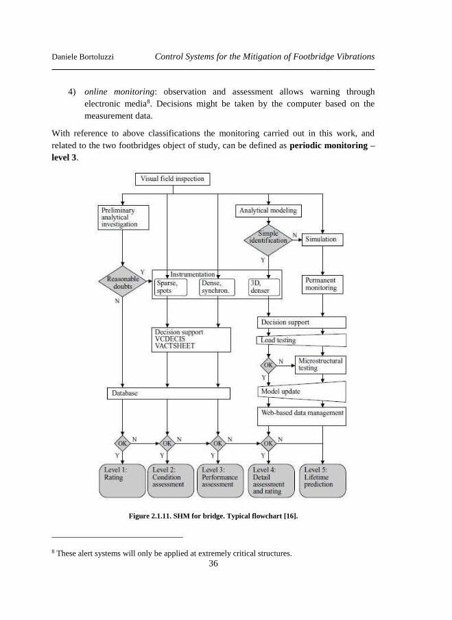
Daniele Bortoluzzi Control Systems for the Mitigation of Footbridge Vibrations
36
4) online monitoring: observation and assessment allows warning through
electronic media8. Decisions might be taken by the computer based on the
measurement data.
With reference to above classifications the monitoring carried out in this work, and
related to the two footbridges object of study, can be defined as periodic monitoring –
level 3.
Figure 2.1.11. SHM for bridge. Typical flowchart [16].
8 These alert systems will only be applied at extremely critical structures.
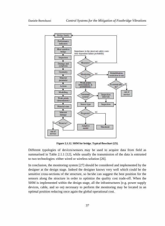
Daniele Bortoluzzi Control Systems for the Mitigation of Footbridge Vibrations
37
Figure 2.1.12. SHM for bridge. Typical flowchart [25].
Different typologies of devices/sensors may be used to acquire data from field as
summarised in Table 2.1.1 [12], while usually the transmission of the data is entrusted
to two technologies: either wired or wireless solution [26].
In conclusion, the monitoring system [27] should be considered and implemented by the
designer at the design stage. Indeed the designer knows very well which could be the
sensitive cross-sections of the structure, so he/she can suggest the best position for the
sensors along the structure in order to optimize the quality cost trade-off. When the
SHM is implemented within the design stage, all the infrastructures (e.g. power supply
devices, cable, and so on) necessary to perform the monitoring may be located in an
optimal position reducing once again the global operational cost.
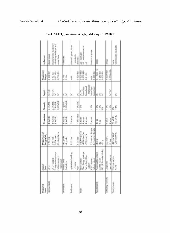
Daniele Bortoluzzi Control Systems for the Mitigation of Footbridge Vibrations
38
Table 2.1.1. Typical sensors employed during a SHM [12].
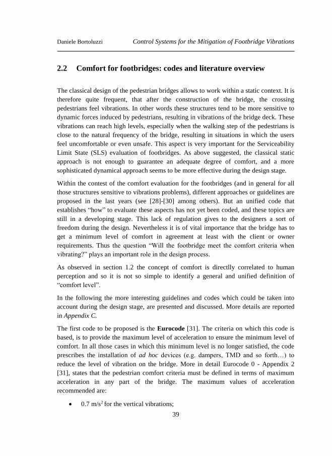
Daniele Bortoluzzi Control Systems for the Mitigation of Footbridge Vibrations
39
2.2 Comfort for footbridges: codes and literature overview
The classical design of the pedestrian bridges allows to work within a static context. It is
therefore quite frequent, that after the construction of the bridge, the crossing
pedestrians feel vibrations. In other words these structures tend to be more sensitive to
dynamic forces induced by pedestrians, resulting in vibrations of the bridge deck. These
vibrations can reach high levels, especially when the walking step of the pedestrians is
close to the natural frequency of the bridge, resulting in situations in which the users
feel uncomfortable or even unsafe. This aspect is very important for the Serviceability
Limit State (SLS) evaluation of footbridges. As above suggested, the classical static
approach is not enough to guarantee an adequate degree of comfort, and a more
sophisticated dynamical approach seems to be more effective during the design stage.
Within the contest of the comfort evaluation for the footbridges (and in general for all
those structures sensitive to vibrations problems), different approaches or guidelines are
proposed in the last years (see [28]-[30] among others). But an unified code that
establishes “how” to evaluate these aspects has not yet been coded, and these topics are
still in a developing stage. This lack of regulation gives to the designers a sort of
freedom during the design. Nevertheless it is of vital importance that the bridge has to
get a minimum level of comfort in agreement at least with the client or owner
requirements. Thus the question “Will the footbridge meet the comfort criteria when
vibrating?” plays an important role in the design process.
As observed in section 1.2 the concept of comfort is directlly correlated to human
perception and so it is not so simple to identify a general and unified definition of
“comfort level”.
In the following the more interesting guidelines and codes which could be taken into
account during the design stage, are presented and discussed. More details are reported
in Appendix C.
The first code to be proposed is the Eurocode [31]. The criteria on which this code is
based, is to provide the maximum level of acceleration to ensure the minimum level of
comfort. In all those cases in which this minimum level is no longer satisfied, the code
prescribes the installation of ad hoc devices (e.g. dampers, TMD and so forth…) to
reduce the level of vibration on the bridge. More in detail Eurocode 0 - Appendix 2
[31], states that the pedestrian comfort criteria must be defined in terms of maximum
acceleration in any part of the bridge. The maximum values of acceleration
recommended are:
0.7 m/s2 for the vertical vibrations;
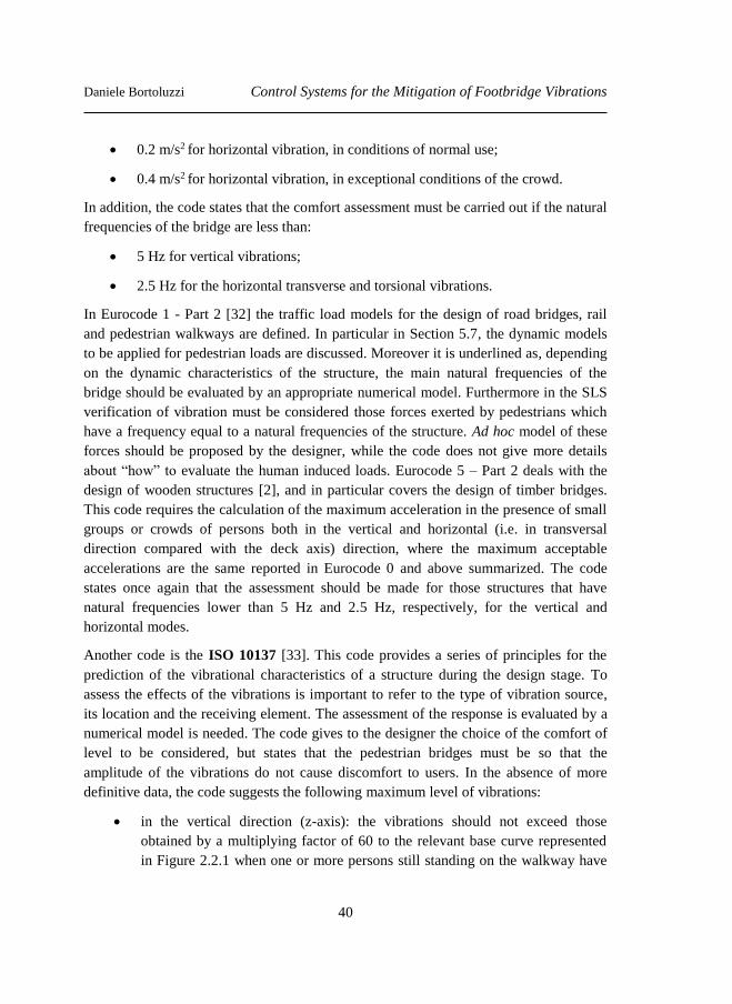
Daniele Bortoluzzi Control Systems for the Mitigation of Footbridge Vibrations
40
0.2 m/s2 for horizontal vibration, in conditions of normal use;
0.4 m/s2 for horizontal vibration, in exceptional conditions of the crowd.
In addition, the code states that the comfort assessment must be carried out if the natural
frequencies of the bridge are less than:
5 Hz for vertical vibrations;
2.5 Hz for the horizontal transverse and torsional vibrations.
In Eurocode 1 - Part 2 [32] the traffic load models for the design of road bridges, rail
and pedestrian walkways are defined. In particular in Section 5.7, the dynamic models
to be applied for pedestrian loads are discussed. Moreover it is underlined as, depending
on the dynamic characteristics of the structure, the main natural frequencies of the
bridge should be evaluated by an appropriate numerical model. Furthermore in the SLS
verification of vibration must be considered those forces exerted by pedestrians which
have a frequency equal to a natural frequencies of the structure. Ad hoc model of these
forces should be proposed by the designer, while the code does not give more details
about “how” to evaluate the human induced loads. Eurocode 5 – Part 2 deals with the
design of wooden structures [2], and in particular covers the design of timber bridges.
This code requires the calculation of the maximum acceleration in the presence of small
groups or crowds of persons both in the vertical and horizontal (i.e. in transversal
direction compared with the deck axis) direction, where the maximum acceptable
accelerations are the same reported in Eurocode 0 and above summarized. The code
states once again that the assessment should be made for those structures that have
natural frequencies lower than 5 Hz and 2.5 Hz, respectively, for the vertical and
horizontal modes.
Another code is the ISO 10137 [33]. This code provides a series of principles for the
prediction of the vibrational characteristics of a structure during the design stage. To
assess the effects of the vibrations is important to refer to the type of vibration source,
its location and the receiving element. The assessment of the response is evaluated by a
numerical model is needed. The code gives to the designer the choice of the comfort of
level to be considered, but states that the pedestrian bridges must be so that the
amplitude of the vibrations do not cause discomfort to users. In the absence of more
definitive data, the code suggests the following maximum level of vibrations:
in the vertical direction (z-axis): the vibrations should not exceed those
obtained by a multiplying factor of 60 to the relevant base curve represented
in Figure 2.2.1 when one or more persons still standing on the walkway have
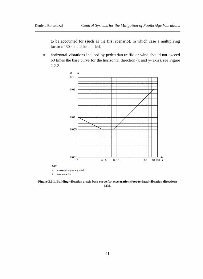
Daniele Bortoluzzi Control Systems for the Mitigation of Footbridge Vibrations
41
to be accounted for (such as the first scenario), in which case a multiplying
factor of 30 should be applied.
horizontal vibrations induced by pedestrian traffic or wind should not exceed
60 times the base curve for the horizontal direction (x and y- axis), see Figure
2.2.2.
Figure 2.2.1. Building vibration z-axis base curve for acceleration (foot-to-head vibration direction)
[33].
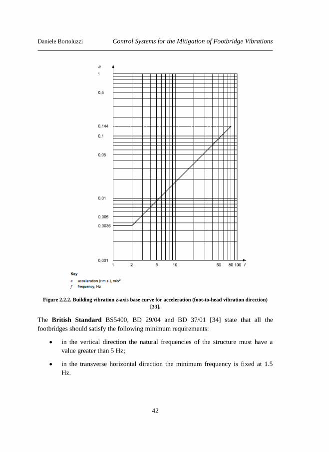
Daniele Bortoluzzi Control Systems for the Mitigation of Footbridge Vibrations
42
Figure 2.2.2. Building vibration z-axis base curve for acceleration (foot-to-head vibration direction)
[33].
The British Standard BS5400, BD 29/04 and BD 37/01 [34] state that all the
footbridges should satisfy the following minimum requirements:
in the vertical direction the natural frequencies of the structure must have a
value greater than 5 Hz;
in the transverse horizontal direction the minimum frequency is fixed at 1.5
Hz.
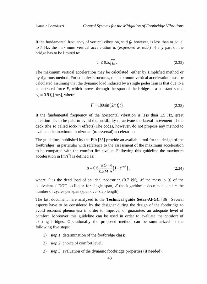
Daniele Bortoluzzi Control Systems for the Mitigation of Footbridge Vibrations
43
If the fundamental frequency of vertical vibration, said f0, however, is less than or equal
to 5 Hz, the maximum vertical acceleration av (expressed as m/s2) of any part of the
bridge has to be limited to:
00.5va f . (2.32)
The maximum vertical acceleration may be calculated either by simplified method or
by rigorous method. For complex structures, the maximum vertical acceleration must be
calculated assuming that the dynamic load induced by a single pedestrian is that due to a
concetrated force F, which moves through the span of the bridge at a constant speed
00.9tv f [m/s], where:
0180sin 2F f t . (2.33)
If the fundamental frequency of the horizontal vibration is less than 1.5 Hz, great
attention has to be paid to avoid the possibility to activate the lateral movement of the
deck (the so called lock-in effects).The codes, however, do not propose any method to
evaluate the maximum horizontal (transversal) acceleration.
The guidelines published by the Fib [35] provide an available tool for the design of the
footbridges, in particular with reference to the assessment of the maximum acceleration
to be compared with the comfort limit value. Following this guideline the maximum
acceleration in [m/s2] is defined as:
0.6 10.5
nGa e
M
, (2.34)
where G is the dead load of an ideal pedestrian (0.7 kN), M the mass in [t] of the
equivalent 1-DOF oscillator for single span, the logarithmic decrement and n the
number of cycles per span (span over step length).
The last document here analyzed is the Technical guide Sétra-AFGC [36]. Several
aspects have to be considered by the designer during the design of the footbridge to
avoid resonant phenomena in order to improve, or guarantee, an adequate level of
comfort. Moreover this guideline can be used in order to evaluate the comfort of
existing bridges. Operationally the proposed method can be summarized in the
following five steps:
1) step 1: determination of the footbridge class;
2) step 2: choice of comfort level;
3) step 3: evaluation of the dynamic footbridge properties (if needed);
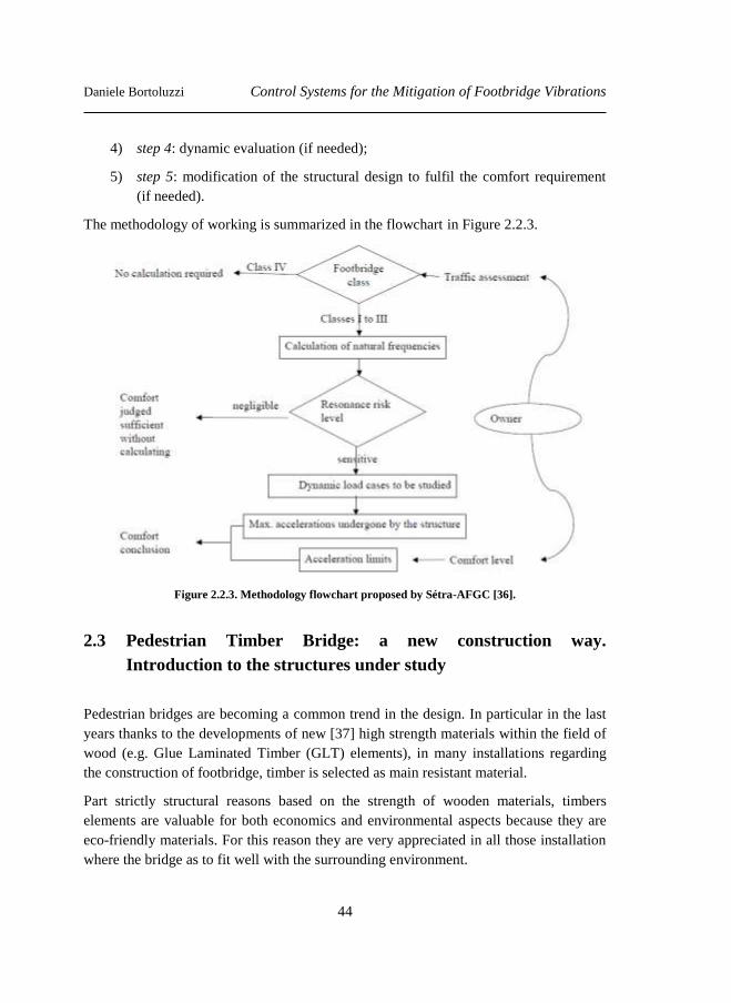
Daniele Bortoluzzi Control Systems for the Mitigation of Footbridge Vibrations
44
4) step 4: dynamic evaluation (if needed);
5) step 5: modification of the structural design to fulfil the comfort requirement
(if needed).
The methodology of working is summarized in the flowchart in Figure 2.2.3.
Figure 2.2.3. Methodology flowchart proposed by Sétra-AFGC [36].
2.3 Pedestrian Timber Bridge: a new construction way.
Introduction to the structures under study
Pedestrian bridges are becoming a common trend in the design. In particular in the last
years thanks to the developments of new [37] high strength materials within the field of
wood (e.g. Glue Laminated Timber (GLT) elements), in many installations regarding
the construction of footbridge, timber is selected as main resistant material.
Part strictly structural reasons based on the strength of wooden materials, timbers
elements are valuable for both economics and environmental aspects because they are
eco-friendly materials. For this reason they are very appreciated in all those installation
where the bridge as to fit well with the surrounding environment.
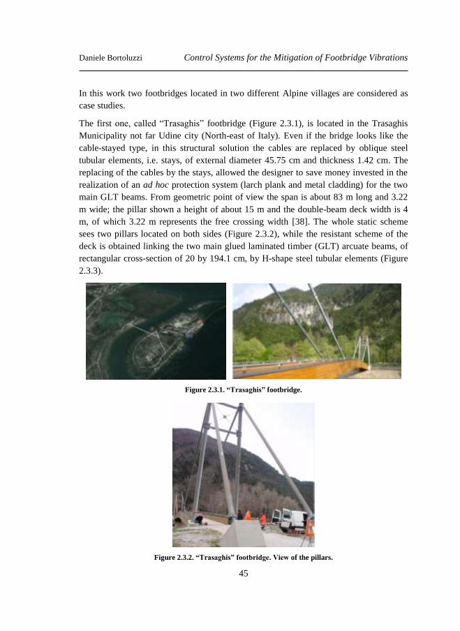
Daniele Bortoluzzi Control Systems for the Mitigation of Footbridge Vibrations
45
In this work two footbridges located in two different Alpine villages are considered as
case studies.
The first one, called “Trasaghis” footbridge (Figure 2.3.1), is located in the Trasaghis
Municipality not far Udine city (North-east of Italy). Even if the bridge looks like the
cable-stayed type, in this structural solution the cables are replaced by oblique steel
tubular elements, i.e. stays, of external diameter 45.75 cm and thickness 1.42 cm. The
replacing of the cables by the stays, allowed the designer to save money invested in the
realization of an ad hoc protection system (larch plank and metal cladding) for the two
main GLT beams. From geometric point of view the span is about 83 m long and 3.22
m wide; the pillar shown a height of about 15 m and the double-beam deck width is 4
m, of which 3.22 m represents the free crossing width [38]. The whole static scheme
sees two pillars located on both sides (Figure 2.3.2), while the resistant scheme of the
deck is obtained linking the two main glued laminated timber (GLT) arcuate beams, of
rectangular cross-section of 20 by 194.1 cm, by H-shape steel tubular elements (Figure
2.3.3).
Figure 2.3.1. “Trasaghis” footbridge.
Figure 2.3.2. “Trasaghis” footbridge. View of the pillars.
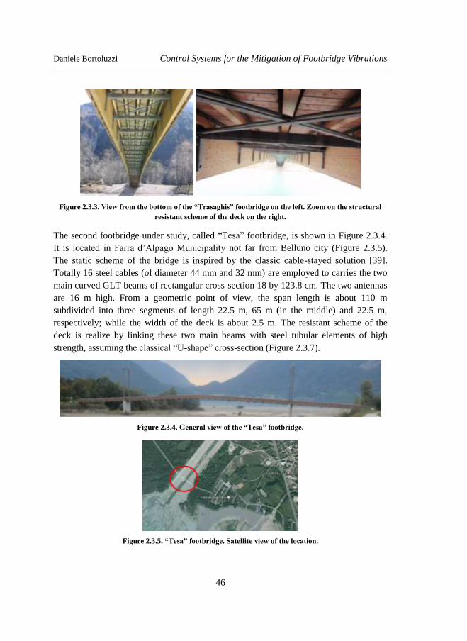
Daniele Bortoluzzi Control Systems for the Mitigation of Footbridge Vibrations
46
Figure 2.3.3. View from the bottom of the “Trasaghis” footbridge on the left. Zoom on the structural
resistant scheme of the deck on the right.
The second footbridge under study, called “Tesa” footbridge, is shown in Figure 2.3.4.
It is located in Farra d’Alpago Municipality not far from Belluno city (Figure 2.3.5).
The static scheme of the bridge is inspired by the classic cable-stayed solution [39].
Totally 16 steel cables (of diameter 44 mm and 32 mm) are employed to carries the two
main curved GLT beams of rectangular cross-section 18 by 123.8 cm. The two antennas
are 16 m high. From a geometric point of view, the span length is about 110 m
subdivided into three segments of length 22.5 m, 65 m (in the middle) and 22.5 m,
respectively; while the width of the deck is about 2.5 m. The resistant scheme of the
deck is realize by linking these two main beams with steel tubular elements of high
strength, assuming the classical “U-shape” cross-section (Figure 2.3.7).
Figure 2.3.4. General view of the “Tesa” footbridge.
Figure 2.3.5. “Tesa” footbridge. Satellite view of the location.
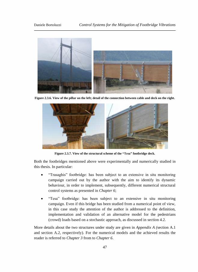
Daniele Bortoluzzi Control Systems for the Mitigation of Footbridge Vibrations
47
Figure 2.3.6. View of the pillar on the left; detail of the connection between cable and deck on the right.
Figure 2.3.7. View of the structural scheme of the “Tesa” footbridge deck.
Both the footbridges mentioned above were experimentally and numerically studied in
this thesis. In particular:
“Trasaghis” footbridge: has been subject to an extensive in situ monitoring
campaign carried out by the author with the aim to identify its dynamic
behaviour, in order to implement, subsequently, different numerical structural
control systems as presented in Chapter 6;
“Tesa” footbridge: has been subject to an extensive in situ monitoring
campaign. Even if this bridge has been studied from a numerical point of view,
in this case study the attention of the author is addressed to the definition,
implementation and validation of an alternative model for the pedestrians
(crowd) loads based on a stochastic approach, as discussed in section 4.2.
More details about the two structures under study are given in Appendix A (section A.1
and section A.2, respectively). For the numerical models and the achieved results the
reader is referred to Chapter 3 from to Chapter 6.
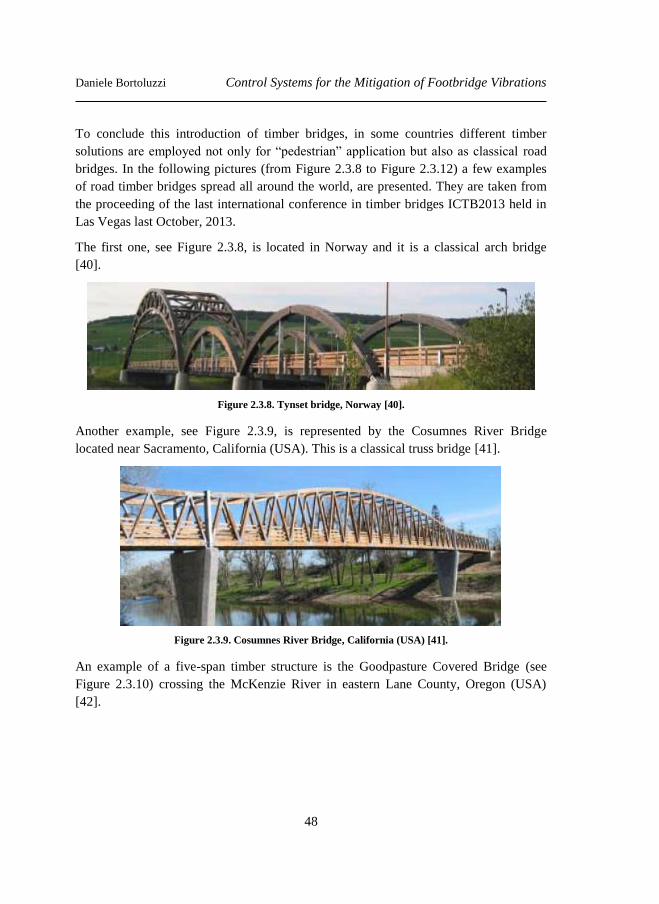
Daniele Bortoluzzi Control Systems for the Mitigation of Footbridge Vibrations
48
To conclude this introduction of timber bridges, in some countries different timber
solutions are employed not only for “pedestrian” application but also as classical road
bridges. In the following pictures (from Figure 2.3.8 to Figure 2.3.12) a few examples
of road timber bridges spread all around the world, are presented. They are taken from
the proceeding of the last international conference in timber bridges ICTB2013 held in
Las Vegas last October, 2013.
The first one, see Figure 2.3.8, is located in Norway and it is a classical arch bridge
[40].
Figure 2.3.8. Tynset bridge, Norway [40].
Another example, see Figure 2.3.9, is represented by the Cosumnes River Bridge
located near Sacramento, California (USA). This is a classical truss bridge [41].
Figure 2.3.9. Cosumnes River Bridge, California (USA) [41].
An example of a five-span timber structure is the Goodpasture Covered Bridge (see
Figure 2.3.10) crossing the McKenzie River in eastern Lane County, Oregon (USA)
[42].
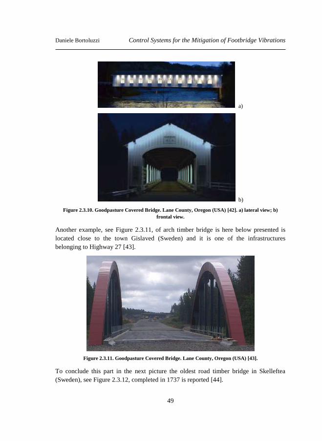
Daniele Bortoluzzi Control Systems for the Mitigation of Footbridge Vibrations
49
a)
b)
Figure 2.3.10. Goodpasture Covered Bridge. Lane County, Oregon (USA) [42]. a) lateral view; b)
frontal view.
Another example, see Figure 2.3.11, of arch timber bridge is here below presented is
located close to the town Gislaved (Sweden) and it is one of the infrastructures
belonging to Highway 27 [43].
Figure 2.3.11. Goodpasture Covered Bridge. Lane County, Oregon (USA) [43].
To conclude this part in the next picture the oldest road timber bridge in Skelleftea
(Sweden), see Figure 2.3.12, completed in 1737 is reported [44].
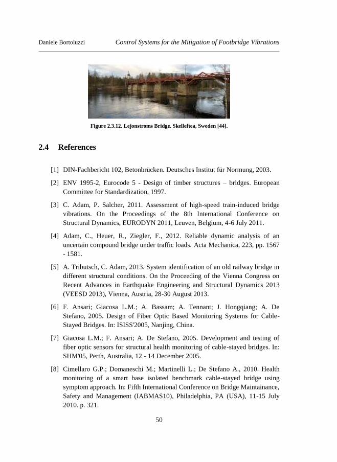
Daniele Bortoluzzi Control Systems for the Mitigation of Footbridge Vibrations
50
Figure 2.3.12. Lejonstroms Bridge. Skelleftea, Sweden [44].
2.4 References
[1] DIN-Fachbericht 102, Betonbrücken. Deutsches Institut für Normung, 2003.
[2] ENV 1995-2, Eurocode 5 - Design of timber structures – bridges. European
Committee for Standardization, 1997.
[3] C. Adam, P. Salcher, 2011. Assessment of high-speed train-induced bridge
vibrations. On the Proceedings of the 8th International Conference on
Structural Dynamics, EURODYN 2011, Leuven, Belgium, 4-6 July 2011.
[4] Adam, C., Heuer, R., Ziegler, F., 2012. Reliable dynamic analysis of an
uncertain compound bridge under traffic loads. Acta Mechanica, 223, pp. 1567
- 1581.
[5] A. Tributsch, C. Adam, 2013. System identification of an old railway bridge in
different structural conditions. On the Proceeding of the Vienna Congress on
Recent Advances in Earthquake Engineering and Structural Dynamics 2013
(VEESD 2013), Vienna, Austria, 28-30 August 2013.
[6] F. Ansari; Giacosa L.M.; A. Bassam; A. Tennant; J. Hongqiang; A. De
Stefano, 2005. Design of Fiber Optic Based Monitoring Systems for Cable-
Stayed Bridges. In: ISISS'2005, Nanjing, China.
[7] Giacosa L.M.; F. Ansari; A. De Stefano, 2005. Development and testing of
fiber optic sensors for structural health monitoring of cable-stayed bridges. In:
SHM'05, Perth, Australia, 12 - 14 December 2005.
[8] Cimellaro G.P.; Domaneschi M.; Martinelli L.; De Stefano A., 2010. Health
monitoring of a smart base isolated benchmark cable-stayed bridge using
symptom approach. In: Fifth International Conference on Bridge Maintainance,
Safety and Management (IABMAS10), Philadelphia, PA (USA), 11-15 July
2010. p. 321.
Daniele Bortoluzzi Control Systems for the Mitigation of Footbridge Vibrations
51
[9] Anil K. Chopra, 1995. Dynamics of Structures, third edition. Prentice Hall,
Englewood Cliffs, New Jersey.
[10] Tom Proulx, 2010. Dynamics of Bridges. Conference Prooceding of the
Society for Experimental Mechanics Series – A conference on Structural
Dynamics, 28th IMAC.
[11] H. Max Irvine, 1981. Cable Structures. The MIT Press Series in Structural
Mechnics. Cambridge, Massachussetts, and London, England.
[12] Wenzel H., 2009. Health Monitoring of Bridges. John Wiley & Sons Ltd, The
Atrium, Southern Gate, Chichester, West Sussex PO19 8 - SQ, England.
[13] Wenzel H., Pichler D., 2005. Ambient Vibration Monitoring. John Wiley &
Sons Ltd, The Atrium, Southern Gate, Chichester, West Sussex PO19 8SQ,
England.
[14] C.F. Beards, 1996. Structural Vibration: Analysis and Damping. Halsted Press,
an imprint of John Wiley & Sons Inc., New York NY.
[15] Ewins, D.J., 2000. Modal Testing: theory, practice and application, 2nd ed.,
Research Studies Press.
[16] Kareem A., Gurley K., 1996. Damping in structures: its evauation and
treatment of uncertainty. Journal of Wind Engineering and Industrial
Aerodynamics, 59, pp. 131-157.
[17] Farrar C. R., Worden K., 2012. Structural Health Monitoring: A Machine
Learning Perspective. Fundamental axioms of structural health monitoring.
John Wiley & Sons, Chichester, UK, November 22, 2012.
[18] Casciati F., Faravelli L., 1991. Fragility analysis of complex structural system,
Research Studies Press, Taunton.
[19] Balkaya,C., Bortoluzzi D., Casciati F., Kostopoluos G., Bogonikolos N., 2012.
System Architecture For An Interactive Database To Structural Control Of
Transport Network Infrastructure: A Case Study Of Railroad Bridge. On the
Proceeding of 5th European Conference on Structural Control – EACS2012,
Genova, Italy 18-20 June 2012.
[20] Faravelli L., Bortoluzzi D., Messervey T.B., Sasek L., 2012. Temperature
Effects On The Response Of The Bridge “ÖBB Brucke Großhaslau”. Invited
contribution - ABC12, Saint Petersburg, Russia, July 1-4, 2012.
Daniele Bortoluzzi Control Systems for the Mitigation of Footbridge Vibrations
52
[21] Casciati S., Faravelli L., Bortoluzzi D., 2013. The Effect Of Temperature
Variability When Monitoring A Railway Bridge. On the proceeding of 11th
International Conference on Recent Advances in Structural Dynamics -
RASD2013, Pisa (ITA).1st – 3rd July 2013.
[22] Casciati F., Casciati S., Faravelli L., Bortoluzzi D., Masservey T.B., 2013.
Estimating Thermal Inertia And Temperature Distribution Consistent With
Monitored Data From A Railway Bridge. On the Proceeding of the 4th
International Conference on Computational Methods in Structural Dynamics &
Earthquake Engineering - COMPDYN2013, Kos Island (GR), 12-14 Jun 2013.
[23] Bortoluzzi D., Casciati S., Faravelli L., 2013. Modeling The Dependency of
Displacement Variability on Thermal Effects. Journal of Vibration and
Control, vol. 19 (15), pp. 2301-2313.
[24] Peeters, B., G. De Roeck, 2001. One-year monitoring of the Z24-Bridge:
environmental effects versus damage events. Journal Of Earthquake
Engineering And Structural Dynamics, 30, pp. 149-171.
[25] Peil U., Mehdianpour M., Frenz M. and Weilert K., 2006. Life time assessment
of bridges In Bridge Maintenance, Safety, Management, Life-Cycle
Performance and Cost. Ed. Cruz PJ, Frangopol DM and Neves LC.
[26] Casciati S., Chen Z., 2011. A multi‐channel wireless connection system for
structural health monitoring applications. Structural Control and Health
Monitoring Journal, 18 (5), pp. 588–600.
[27] SAMCO – Guidelines for Structural Control, 2006. www.samco.org
[28] Oeding, 1961. Verkehrsanalyse Fußgänger, Stadt Stuttgart Planungsamt, Abt.
Verkehr [in German].
[29] HiVoSS Design of Footbridges – guideline, 2008. Project: RFS2-CT-2007-
00033 – EN02.
[30] HiVoSS Design of Footbridges – guideline, 2008. Project: RFS2-CT-2007-
00033 – EN03.
[31] Eurocode 0 - Appendix A2, Basis of Structural Design, EN 1990.
[32] Eurocode 1 - Part 3, Actions on structures. UNI ENV 1991-3, September 1998.
[33] ISO 10137, Bases for design of structures - Serviceability of buildings and
walkways against vibration, 2007.
Daniele Bortoluzzi Control Systems for the Mitigation of Footbridge Vibrations
53
[34] BS5400, Part 2, Appendix C, Vibration Serviceability Requirements for Foot
and Cycle Track Bridges. British Standards Institution, 1978.
[35] Guidelines for the design of footbridges. Fib bulletin 32, November 2005.
[36] Footbridges: assessment of vibrational behaviour of footbridges under
pedestrian loading - Technical guide, 2006 – Sétra-AFGC.
[37] Pisano A., Fuschi P, De Domenico D, 2014. Limit Analysis: A Layered
Approach for Composite Laminates , Direct Methods for Limit States in
Structures and Materials,Springer Science+Business Media B.V., Dordrecht
(DEU), pp. 23-56, ISBN: 978-94-007-6826-0.
[38] Casciati S., Faravelli L. and Bortoluzzi D., 2013. Pedestrian timber bridges:
experimental investigation and modelling. On the Proceeding of the 10th
International Conference on Damage Assessment of Structures - DAMAS 2013.
Trinity College Dublin Ireland, July 8-10 2013.
[39] Bortoluzzi D., Casciati S., Faravelli L., 2013. Testing the effects of walking
and running on an existing timber pedestrian bridge. On the Proceeding of the
9th International Conference on Structural Dynamics - EURODYN 2014.
Porto, Portugal, 30 June – 2 July 2014.
[40] Malo K.A., Ostrycharczyk A., Barli R., Hakvåg I., 2013. On development of
network arch bridges in timber. On the Proceeding of 2nd International
Conference on Timber Bridges 2013 – ICTB2013, Las Vegas, Nevada USA,
September-October, 2013.
[41] Gilham P.C., 2013. Stretching the Limits, Four Timber Bridge Case Studies.
On the Proceeding of 2nd International Conference on Timber Bridges 2013 –
ICTB2013, Las Vegas, Nevada USA, September-October, 2013.
[42] Ausland G.W., La Morticella. T., 2013.Goodpasture Covered Bridge
Rehabilitation. On the Proceeding of 2nd International Conference on Timber
Bridges 2013 – ICTB2013, Las Vegas, Nevada USA, September-October,
2013.
[43] Ekholm, K., Nilsson, P., Johansson, E., 2013. Case Study Of The Longest
Single Span Timber Bridge For Highway Loads In Sweden. On the Proceeding
of 2nd International Conference on Timber Bridges 2013 – ICTB2013, Las
Vegas, Nevada USA, September-October, 2013.
[44] www.tt-forums.net

Daniele Bortoluzzi Control Systems for the Mitigation of Footbridge Vibrations
54
Daniele Bortoluzzi Control Systems for the Mitigation of Footbridge Vibrations
55
Chapter 3 Experimental campaign and numerical
modeling
In this chapter the numerical models of the two pedestrian bridges under study (section
2.3) are presented. For more details about the pedestrian bridges the reader is referred to
Appendix A.
All the structural models are developed within the theory of Finite Element Model
(FEM) [1]. The code adopted is developed by MSC Marc software-house. In particular
the graphical interface called MENTAT2010 [2] is used. This software allows one a
complete solution (pre-processing solution and post-processing solution) for implicit
nonlinear Finite Element Analysis (FEA). It allows one to accurately simulate the
response of structures under static, dynamic and multi-physics loading scenarios.
Marc’s versatility in modelling nonlinear material behaviours and transient
environmental conditions makes it an efficient tool for the design of structural systems.
Moreover it allows the user to define the ad hoc functions for boundary conditions,
loads configuration and so forth…
3.1 Experimental campaign
In this section the experimental campaigns carried out in situ for the two structures
under study are presented. It is worth underlining that these tests are a must in view of
defining more realistic numerical models to represent the dynamic behaviour of the
footbridges. In particular the calibration and validation of the FE models will be
entrusted to the comparison of the responses of the footbridges under wind loads
acquired in situ, with the responses achieved by the implemented numerical models.
Indeed, in this particular application, the loads associated to the wind can be regarded as
“ambient vibration” or “background noise”. During the experimental campaigns, long
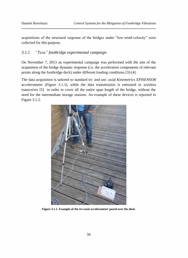
Daniele Bortoluzzi Control Systems for the Mitigation of Footbridge Vibrations
56
acquisitions of the structural response of the bridges under “low-wind-velocity” were
collected for this purpose.
3.1.1 “Tesa” footbridge experimental campaign
On November 7, 2013 an experimental campaign was performed with the aim of the
acquisition of the bridge dynamic response (i.e. the acceleration components of relevant
points along the footbridge deck) under different loading conditions [3]-[4].
The data acquisition is tailored to standard tri- and uni- axial Kinemetrics EPISENSOR
accelerometer (Figure 3.1.1), while the data transmission is entrusted to wireless
transceiver [5] in order to cover all the entire span length of the bridge, without the
need for the intermediate storage stations. An example of these devices is reported in
Figure 3.1.2.
Figure 3.1.1. Example of the tri-axial accelerometer posed over the deck.
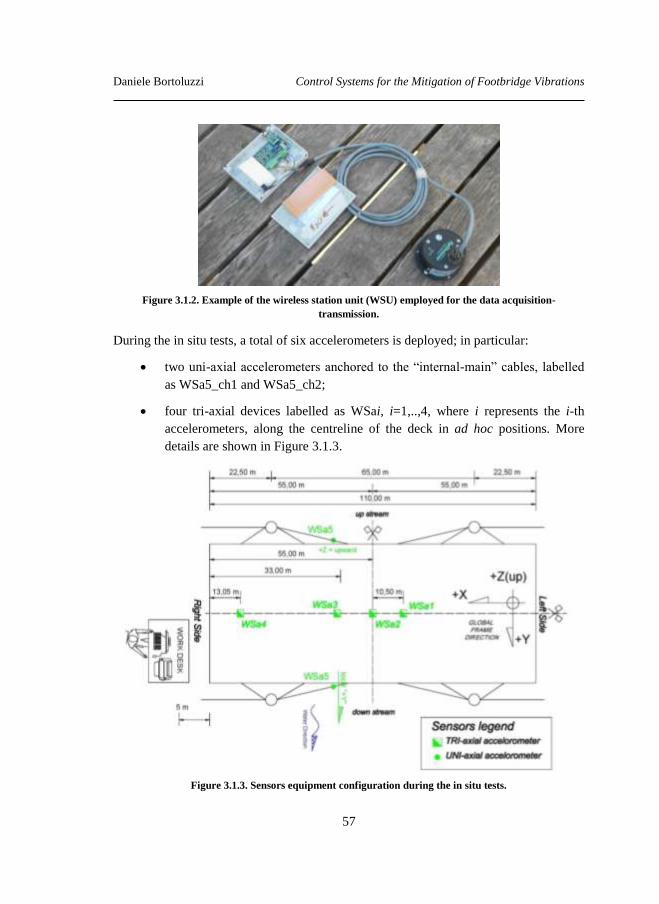
Daniele Bortoluzzi Control Systems for the Mitigation of Footbridge Vibrations
57
Figure 3.1.2. Example of the wireless station unit (WSU) employed for the data acquisition-
transmission.
During the in situ tests, a total of six accelerometers is deployed; in particular:
two uni-axial accelerometers anchored to the “internal-main” cables, labelled
as WSa5_ch1 and WSa5_ch2;
four tri-axial devices labelled as WSai, i=1,..,4, where i represents the i-th
accelerometers, along the centreline of the deck in ad hoc positions. More
details are shown in Figure 3.1.3.
Figure 3.1.3. Sensors equipment configuration during the in situ tests.
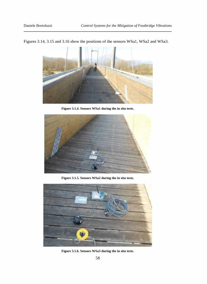
Daniele Bortoluzzi Control Systems for the Mitigation of Footbridge Vibrations
58
Figures 3.14, 3.15 and 3.16 show the positions of the sensors WSa1, WSa2 and WSa3.
Figure 3.1.4. Sensors WSa1 during the in situ tests.
Figure 3.1.5. Sensors WSa2 during the in situ tests.
Figure 3.1.6. Sensors WSa3 during the in situ tests.
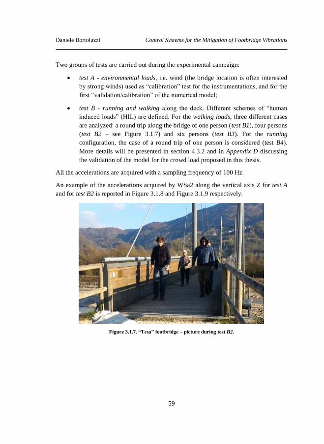
Daniele Bortoluzzi Control Systems for the Mitigation of Footbridge Vibrations
59
Two groups of tests are carried out during the experimental campaign:
test A - environmental loads, i.e. wind (the bridge location is often interested
by strong winds) used as “calibration” test for the instrumentations, and for the
first “validation/calibration” of the numerical model;
test B - running and walking along the deck. Different schemes of “human
induced loads” (HIL) are defined. For the walking loads, three different cases
are analyzed: a round trip along the bridge of one person (test B1), four persons
(test B2 – see Figure 3.1.7) and six persons (test B3). For the running
configuration, the case of a round trip of one person is considered (test B4).
More details will be presented in section 4.3.2 and in Appendix D discussing
the validation of the model for the crowd load proposed in this thesis.
All the accelerations are acquired with a sampling frequency of 100 Hz.
An example of the accelerations acquired by WSa2 along the vertical axis Z for test A
and for test B2 is reported in Figure 3.1.8 and Figure 3.1.9 respectively.
Figure 3.1.7. “Tesa” footbridge – picture during test B2.
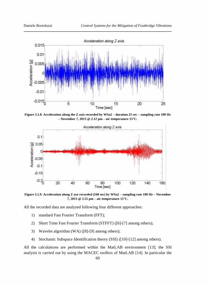
Daniele Bortoluzzi Control Systems for the Mitigation of Footbridge Vibrations
60
Figure 3.1.8. Acceleration along the Z axis recorded by WSa2 – duration 25 sec – sampling rate 100 Hz
– November 7, 2013 @ 2.12 pm – air temperature 15°C.
Figure 3.1.9. Acceleration along Z axe recorded (160 sec) by WSa2 – sampling rate 100 Hz – November
7, 2013 @ 2.55 pm – air temperature 15°C.
All the recorded data are analyzed following four different approaches:
1) standard Fast Fourier Transform (FFT);
2) Short Time Fast Fourier Transform (STFFT) ([6]-[7] among others);
3) Wavelet algorithm (WA) ([8]-[9] among others);
4) Stochastic Subspace Identification theory (SSI) ([10]-[12] among others).
All the calculations are performed within the MatLAB environment [13]; the SSI
analysis is carried out by using the MACEC toolbox of MatLAB [14]. In particular the
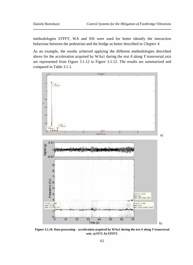
Daniele Bortoluzzi Control Systems for the Mitigation of Footbridge Vibrations
61
methodologies STFFT, WA and SSI were used for better identify the interaction
behaviour between the pedestrian and the bridge as better described in Chapter 4.
As an example, the results achieved applying the different methodologies described
above for the acceleration acquired by WAa1 during the test A along Y transversal axis
are represented from Figure 3.1.12 to Figure 3.1.12. The results are summarized and
compared in Table 3.1.1.
a)
b)
Figure 3.1.10. Data processing – acceleration acquired by WAa1 during the test A along Y transversal
axis. a) FFT; b) STFFT.
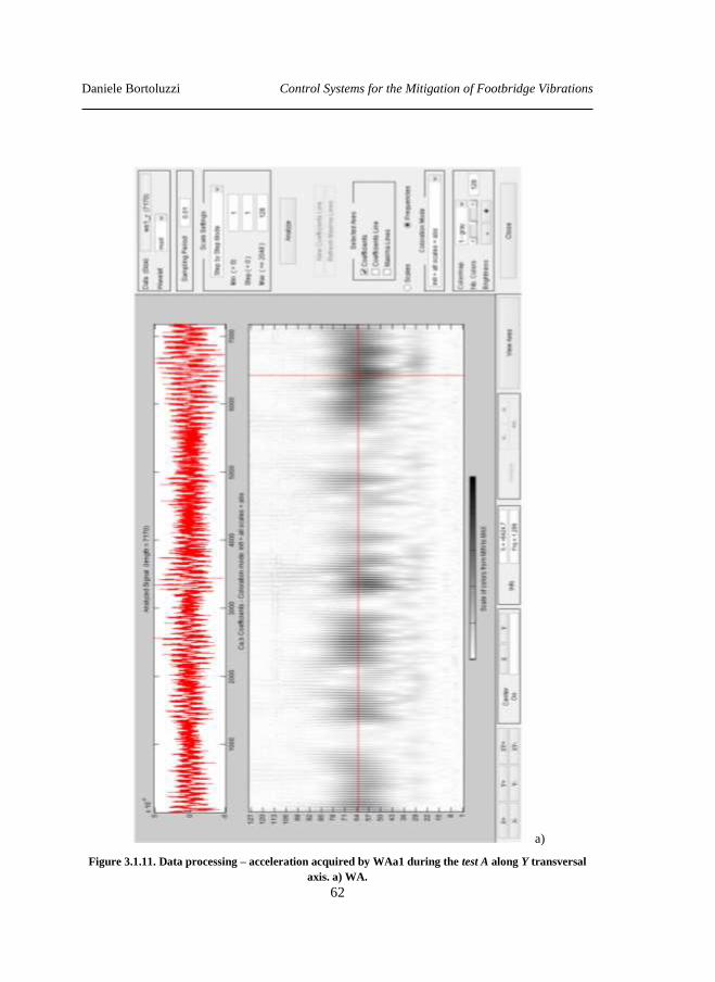
Daniele Bortoluzzi Control Systems for the Mitigation of Footbridge Vibrations
62
a)
Figure 3.1.11. Data processing – acceleration acquired by WAa1 during the test A along Y transversal
axis. a) WA.
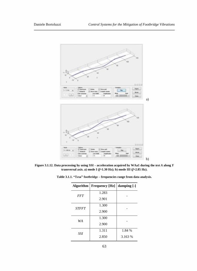
Daniele Bortoluzzi Control Systems for the Mitigation of Footbridge Vibrations
63
a)
b)
Figure 3.1.12. Data processing by using SSI – acceleration acquired by WAa1 during the test A along Y
transversal axis. a) mode I (f=1.30 Hz); b) mode III (f=2.85 Hz).
Table 3.1.1. “Tesa” footbridge – frequencies range from data analysis.
Algorithm Frequency [Hz] damping [-]
FFT 1.283
2.901 -
STFFT 1.300
2.900 -
WA 1.300
2.900 -
SSI 1.311
2.850
1.84 %
3.163 %
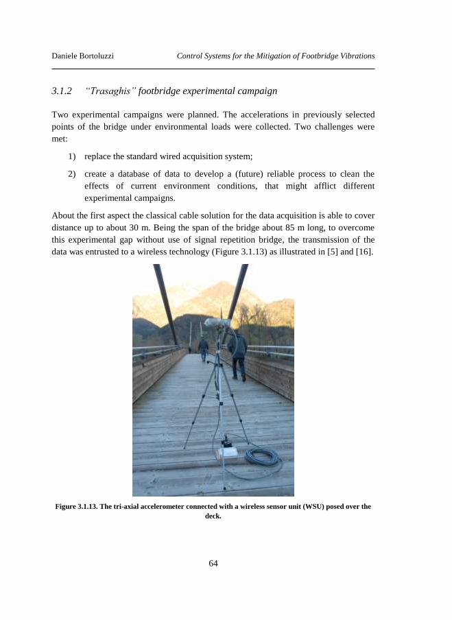
Daniele Bortoluzzi Control Systems for the Mitigation of Footbridge Vibrations
64
3.1.2 “Trasaghis” footbridge experimental campaign
Two experimental campaigns were planned. The accelerations in previously selected
points of the bridge under environmental loads were collected. Two challenges were
met:
1) replace the standard wired acquisition system;
2) create a database of data to develop a (future) reliable process to clean the
effects of current environment conditions, that might afflict different
experimental campaigns.
About the first aspect the classical cable solution for the data acquisition is able to cover
distance up to about 30 m. Being the span of the bridge about 85 m long, to overcome
this experimental gap without use of signal repetition bridge, the transmission of the
data was entrusted to a wireless technology (Figure 3.1.13) as illustrated in [5] and [16].
Figure 3.1.13. The tri-axial accelerometer connected with a wireless sensor unit (WSU) posed over the
deck.
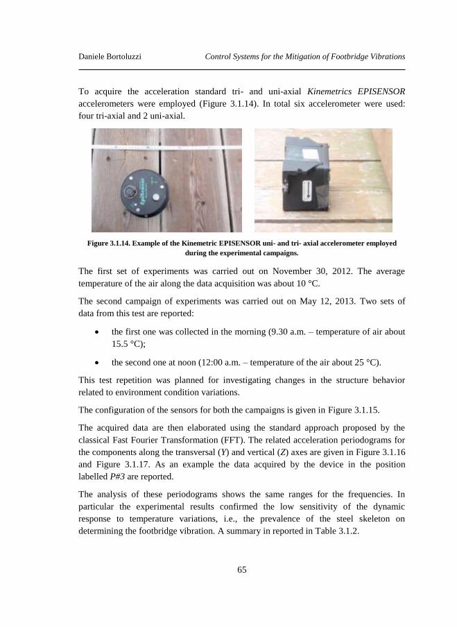
Daniele Bortoluzzi Control Systems for the Mitigation of Footbridge Vibrations
65
To acquire the acceleration standard tri- and uni-axial Kinemetrics EPISENSOR
accelerometers were employed (Figure 3.1.14). In total six accelerometer were used:
four tri-axial and 2 uni-axial.
Figure 3.1.14. Example of the Kinemetric EPISENSOR uni- and tri- axial accelerometer employed
during the experimental campaigns.
The first set of experiments was carried out on November 30, 2012. The average
temperature of the air along the data acquisition was about 10 °C.
The second campaign of experiments was carried out on May 12, 2013. Two sets of
data from this test are reported:
the first one was collected in the morning (9.30 a.m. – temperature of air about
15.5 °C);
the second one at noon (12:00 a.m. – temperature of the air about 25 °C).
This test repetition was planned for investigating changes in the structure behavior
related to environment condition variations.
The configuration of the sensors for both the campaigns is given in Figure 3.1.15.
The acquired data are then elaborated using the standard approach proposed by the
classical Fast Fourier Transformation (FFT). The related acceleration periodograms for
the components along the transversal (Y) and vertical (Z) axes are given in Figure 3.1.16
and Figure 3.1.17. As an example the data acquired by the device in the position
labelled P#3 are reported.
The analysis of these periodograms shows the same ranges for the frequencies. In
particular the experimental results confirmed the low sensitivity of the dynamic
response to temperature variations, i.e., the prevalence of the steel skeleton on
determining the footbridge vibration. A summary in reported in Table 3.1.2.
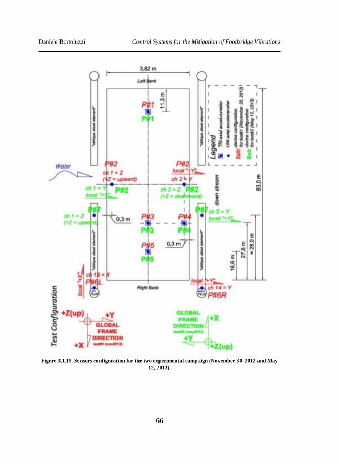
Daniele Bortoluzzi Control Systems for the Mitigation of Footbridge Vibrations
66
Figure 3.1.15. Sensors configuration for the two experimental campaign (November 30, 2012 and May
12, 2013).
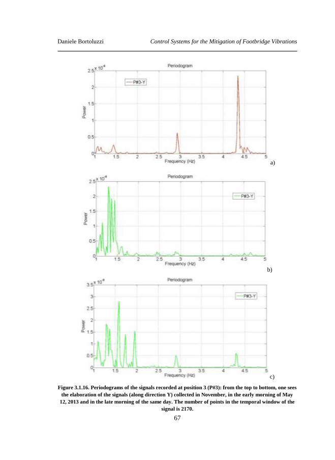
Daniele Bortoluzzi Control Systems for the Mitigation of Footbridge Vibrations
67
a)
b)
c)
Figure 3.1.16. Periodograms of the signals recorded at position 3 (P#3): from the top to bottom, one sees
the elaboration of the signals (along direction Y) collected in November, in the early morning of May
12, 2013 and in the late morning of the same day. The number of points in the temporal window of the
signal is 2170.
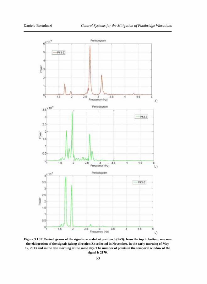
Daniele Bortoluzzi Control Systems for the Mitigation of Footbridge Vibrations
68
a)
b)
c)
Figure 3.1.17. Periodograms of the signals recorded at position 3 (P#3): from the top to bottom, one sees
the elaboration of the signals (along direction Z) collected in November, in the early morning of May
12, 2013 and in the late morning of the same day. The number of points in the temporal window of the
signal is 2170.
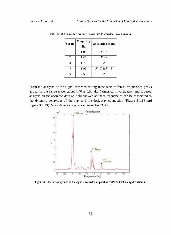
Daniele Bortoluzzi Control Systems for the Mitigation of Footbridge Vibrations
69
Table 3.1.2. Frequency ranges “Trasaghis” footbridge – main results.
Set ID Frequency
[Hz] Oscillation plane
1 1.05 X – Z
2 1.40 X - Y
3 1.75 Z
4 1.96 X - Y & X – Z
5 2.55 Z
From the analysis of the signal recorded during these tests different frequencies peaks
appear in the range under about 1.40 ± 1.50 Hz. Numerical investigation and focused
analysis on the acquired data on field showed as these frequencies can be associated to
the dynamic behaviour of the stay and the deck-stay connection (Figure 3.1.18 and
Figure 3.1.19). More details are provided in section 3.3.2.
Figure 3.1.18. Periodograms of the signals recorded at position 7 (P#7): FFT along direction Y.
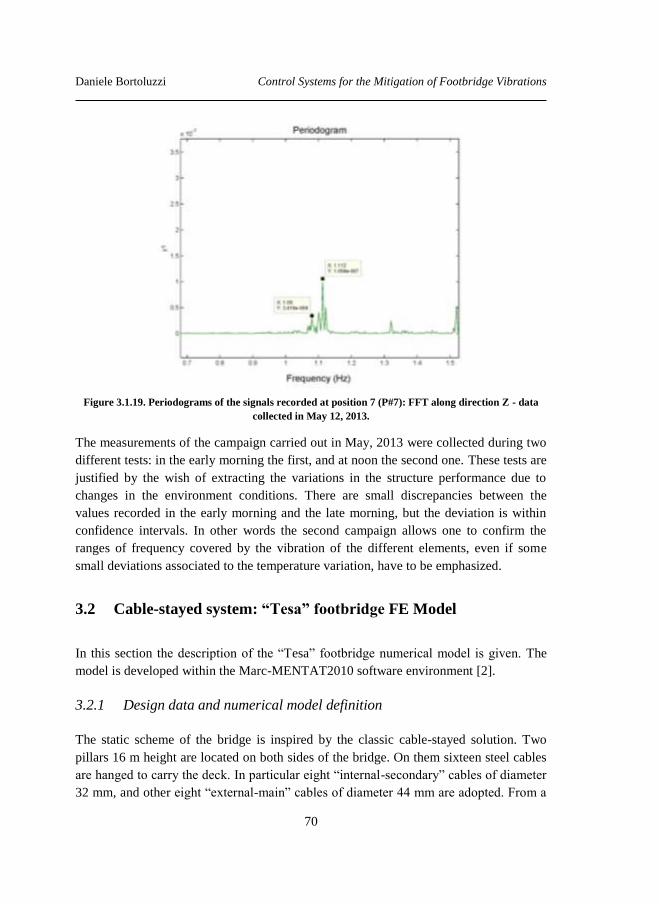
Daniele Bortoluzzi Control Systems for the Mitigation of Footbridge Vibrations
70
Figure 3.1.19. Periodograms of the signals recorded at position 7 (P#7): FFT along direction Z - data
collected in May 12, 2013.
The measurements of the campaign carried out in May, 2013 were collected during two
different tests: in the early morning the first, and at noon the second one. These tests are
justified by the wish of extracting the variations in the structure performance due to
changes in the environment conditions. There are small discrepancies between the
values recorded in the early morning and the late morning, but the deviation is within
confidence intervals. In other words the second campaign allows one to confirm the
ranges of frequency covered by the vibration of the different elements, even if some
small deviations associated to the temperature variation, have to be emphasized.
3.2 Cable-stayed system: “Tesa” footbridge FE Model
In this section the description of the “Tesa” footbridge numerical model is given. The
model is developed within the Marc-MENTAT2010 software environment [2].
3.2.1 Design data and numerical model definition
The static scheme of the bridge is inspired by the classic cable-stayed solution. Two
pillars 16 m height are located on both sides of the bridge. On them sixteen steel cables
are hanged to carry the deck. In particular eight “internal-secondary” cables of diameter
32 mm, and other eight “external-main” cables of diameter 44 mm are adopted. From a
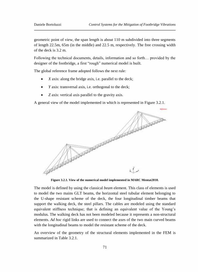
Daniele Bortoluzzi Control Systems for the Mitigation of Footbridge Vibrations
71
geometric point of view, the span length is about 110 m subdivided into three segments
of length 22.5m, 65m (in the middle) and 22.5 m, respectively. The free crossing width
of the deck is 3.2 m.
Following the technical documents, details, information and so forth… provided by the
designer of the footbridge, a first “rough” numerical model is built.
The global reference frame adopted follows the next rule:
X axis: along the bridge axis, i.e. parallel to the deck;
Y axis: transversal axis, i.e. orthogonal to the deck;
Z axis: vertical axis parallel to the gravity axis.
A general view of the model implemented in which is represented in Figure 3.2.1.
Figure 3.2.1. View of the numerical model implemented in MARC Mentat2010.
The model is defined by using the classical beam element. This class of elements is used
to model the two mains GLT beams, the horizontal steel tubular element belonging to
the U-shape resistant scheme of the deck, the four longitudinal timber beams that
support the walking deck, the steel pillars. The cables are modeled using the standard
equivalent stiffness technique; that is defining an equivalent value of the Young’s
modulus. The walking deck has not been modeled because it represents a non-structural
elements. Ad hoc rigid links are used to connect the axes of the two main curved beams
with the longitudinal beams to model the resistant scheme of the deck.
An overview of the geometry of the structural elements implemented in the FEM is
summarized in Table 3.2.1.
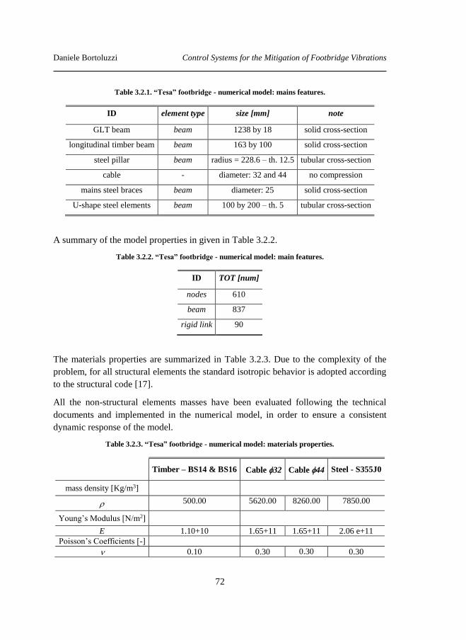
Daniele Bortoluzzi Control Systems for the Mitigation of Footbridge Vibrations
72
Table 3.2.1. “Tesa” footbridge - numerical model: mains features.
ID element type size [mm] note
GLT beam beam 1238 by 18 solid cross-section
longitudinal timber beam beam 163 by 100 solid cross-section
steel pillar beam radius = 228.6 – th. 12.5 tubular cross-section
cable - diameter: 32 and 44 no compression
mains steel braces beam diameter: 25 solid cross-section
U-shape steel elements beam 100 by 200 – th. 5 tubular cross-section
A summary of the model properties in given in Table 3.2.2.
Table 3.2.2. “Tesa” footbridge - numerical model: main features.
ID TOT [num]
nodes 610
beam 837
rigid link 90
The materials properties are summarized in Table 3.2.3. Due to the complexity of the
problem, for all structural elements the standard isotropic behavior is adopted according
to the structural code [17].
All the non-structural elements masses have been evaluated following the technical
documents and implemented in the numerical model, in order to ensure a consistent
dynamic response of the model.
Table 3.2.3. “Tesa” footbridge - numerical model: materials properties.
Timber – BS14 & BS16 Cable 32 Cable 44 Steel - S355J0
mass density [Kg/m3]
500.00 5620.00 8260.00 7850.00
Young’s Modulus [N/m2]
E 1.10+10 1.65+11 1.65+11 2.06 e+11
Poisson’s Coefficients [-]
0.10 0.30 0.30 0.30
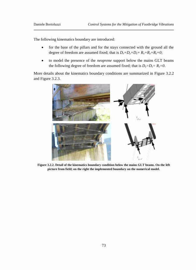
Daniele Bortoluzzi Control Systems for the Mitigation of Footbridge Vibrations
73
The following kinematics boundary are introduced:
for the base of the pillars and for the stays connected with the ground all the
degree of freedom are assumed fixed; that is Dx=Dy=Dz= Rx=Ry=Rz=0;
to model the presence of the neoprene support below the mains GLT beams
the following degree of freedom are assumed fixed; that is Dy=Dz= Rz=0.
More details about the kinematics boundary conditions are summarized in Figure 3.2.2
and Figure 3.2.3.
Figure 3.2.2. Detail of the kinematics boundary condition below the mains GLT beams. On the left
picture from field; on the right the implemented boundary on the numerical model.
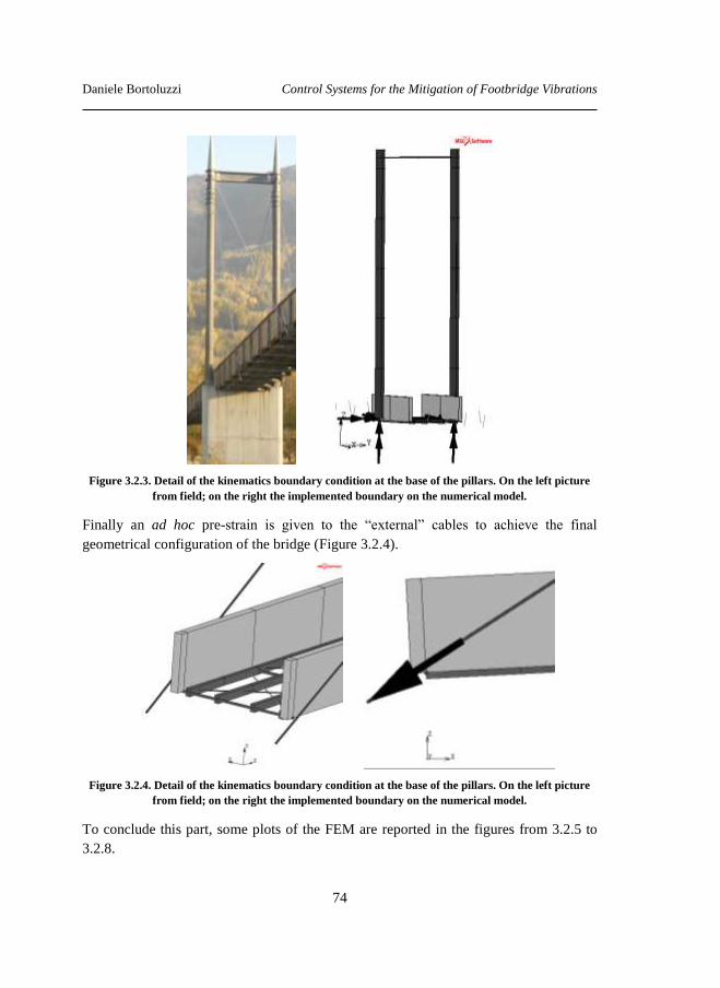
Daniele Bortoluzzi Control Systems for the Mitigation of Footbridge Vibrations
74
Figure 3.2.3. Detail of the kinematics boundary condition at the base of the pillars. On the left picture
from field; on the right the implemented boundary on the numerical model.
Finally an ad hoc pre-strain is given to the “external” cables to achieve the final
geometrical configuration of the bridge (Figure 3.2.4).
Figure 3.2.4. Detail of the kinematics boundary condition at the base of the pillars. On the left picture
from field; on the right the implemented boundary on the numerical model.
To conclude this part, some plots of the FEM are reported in the figures from 3.2.5 to
3.2.8.
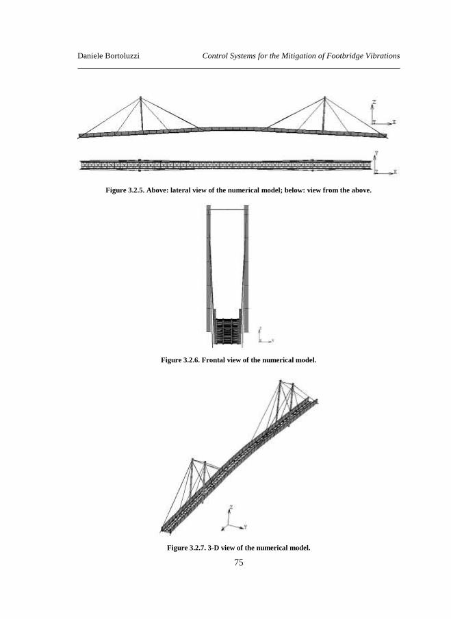
Daniele Bortoluzzi Control Systems for the Mitigation of Footbridge Vibrations
75
Figure 3.2.5. Above: lateral view of the numerical model; below: view from the above.
Figure 3.2.6. Frontal view of the numerical model.
Figure 3.2.7. 3-D view of the numerical model.

Daniele Bortoluzzi Control Systems for the Mitigation of Footbridge Vibrations
76
Figure 3.2.8. View of the deck. On the left 3-D view; on the right cross-section view.
In order to take into account the geometric non linearity due to the presence of the
cables, the “large strain” option has been activated in the software configuration.
It is worth underlining that, even if the whole general dynamic problems is not linear
due to the geometric non linearity introduced by the cables, all the dynamic analysis are
conducted within small oscillations around the deformed configuration of equilibrium
achieved by the bridge.
3.2.2 FE Model refinement and validation
In order to calibrate and validate the numerical model developed, all the data recorded
on the field during test A (section 3.1.1) are analyzed following the standard Fast
Fourier Transform (FFT) approach.
The results achieved for the acceleration acquired by WAa1 during the test A along the
Y transversal axis are represented in Figure 3.2.9. The related results are summarized
and compared in Table 3.2.4.
Based on the results achieved analysing the data acquired on field, the numerical model
previously defined has been refined (e.g. the nodal mass associated to the non-structural
elements has been modified) until the dynamic modal analysis associated to the FEM
“match well” with the experimental evidence.
The comparison between the analysis of the data coming from the field and the refined
numerical model is reported in Figure 3.2.10.
As observed previously even if this bridge has been subject to an extensive study both
from the numerical point of view and from the analysis of the data acquired during the
in situ monitoring campaign, the attention on the “Tesa” footbridge is mainly addressed
to the definition, implementation and validation of a model for the pedestrian loads.
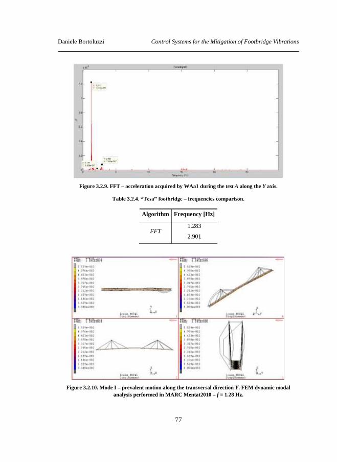
Daniele Bortoluzzi Control Systems for the Mitigation of Footbridge Vibrations
77
Figure 3.2.9. FFT – acceleration acquired by WAa1 during the test A along the Y axis.
Table 3.2.4. “Tesa” footbridge – frequencies comparison.
Algorithm Frequency [Hz]
FFT 1.283
2.901
Figure 3.2.10. Mode I – prevalent motion along the transversal direction Y. FEM dynamic modal
analysis performed in MARC Mentat2010 – f = 1.28 Hz.
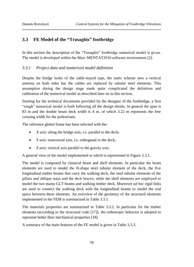
Daniele Bortoluzzi Control Systems for the Mitigation of Footbridge Vibrations
78
3.3 FE Model of the “Trasaghis” footbridge
In this section the description of the “Trasaghis” footbridge numerical model is given.
The model is developed within the Marc-MENTAT2010 software environment [2].
3.3.1 Project data and numerical model definition
Despite the bridge looks of the cable-stayed type, the static scheme sees a vertical
antenna on both sides but the cables are replaced by tubular steel elements. This
assumption during the design stage made quite complicated the definition and
calibration of the numerical model as described later on in this section.
Starting for the technical documents provided by the designer of the footbridge, a first
“rough” numerical model is built following all the design details. In general the span is
83 m and the double beam deck width is 4 m, of which 3.22 m represents the free
crossing width for the pedestrians.
The reference global frame has been selected with the:
X axis: along the bridge axis, i.e. parallel to the deck;
Y axis: transversal axis, i.e. orthogonal to the deck;
Z axis: vertical axis parallel to the gravity axis.
A general view of the model implemented in which is represented in Figure 3.3.1.
The model is composed by classical beam and shell elements. In particular the beam
elements are used to model the H-shape steel tubular element of the deck, the five
longitudinal timber beams that carry the walking deck, the steel tubular elements of the
pillars and oblique stays and the deck braces; while the shell elements are employed to
model the two mains GLT beams and walking timber deck. Moreover ad hoc rigid links
are used to connect the walking deck with the longitudinal beams to model the real
space between these elements. An overview of the geometry of the structural elements
implemented in the FEM is summarized in Table 3.3.1.
The materials properties are summarized in Table 3.3.2. In particular for the timber
elements (according to the structural code [17]), the orthotropic behavior is adopted to
represent better their mechanical properties [18].
A summary of the main features of the FE model is given in Table 3.3.3.
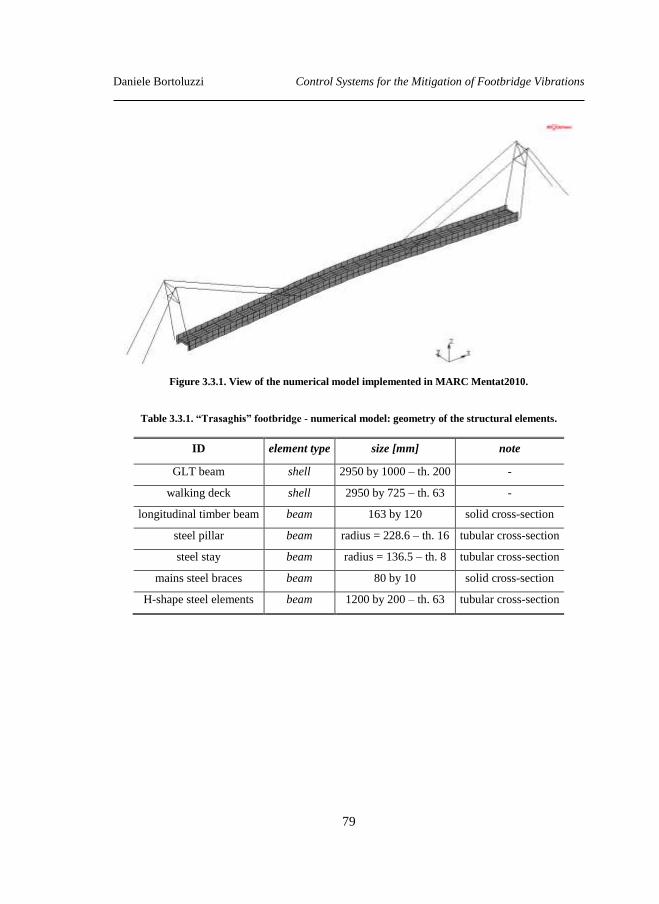
Daniele Bortoluzzi Control Systems for the Mitigation of Footbridge Vibrations
79
Figure 3.3.1. View of the numerical model implemented in MARC Mentat2010.
Table 3.3.1. “Trasaghis” footbridge - numerical model: geometry of the structural elements.
ID element type size [mm] note
GLT beam shell 2950 by 1000 – th. 200 -
walking deck shell 2950 by 725 – th. 63 -
longitudinal timber beam beam 163 by 120 solid cross-section
steel pillar beam radius = 228.6 – th. 16 tubular cross-section
steel stay beam radius = 136.5 – th. 8 tubular cross-section
mains steel braces beam 80 by 10 solid cross-section
H-shape steel elements beam 1200 by 200 – th. 63 tubular cross-section
Daniele Bortoluzzi Control Systems for the Mitigation of Footbridge Vibrations
80
Table 3.3.2. “Trasaghis” footbridge - numerical model: materials properties.
Timber - GL28c Timber - GL24c Steel - S355JR
mass density [Kg/m3]
509.68 509.68 7645.26
Young’s Modulus [N/m2]
E1 1.26e+10 1.16e+10
2.10e+11 E2 3.90e+08 3.20e+08
E3 3.90e+08 3.20e+08
Poisson’s Coefficients [-]
1 0.40 0.40
0.30 2 0.40 0.40
3 0.40 0.40
Shear’s Modulus [N/m2]
G12 7.20+08 5.90+08 8.10e+10 G23 7.20+08 5.90+08
G31 7.20+08 5.90+08
Table 3.3.3. “Trasaghis” footbridge - numerical model: main features.
ID TOT [num]
nodes 724
beam 572
shell 352
rigid link 145
For the kinematics boundary conditions the following assumptions are assumed:
for the base of the pillars and for the stays connected with the ground all the
degree of freedom are assumed fixed; that is Dx=Dy=Dz= Rx=Ry=Rz=0;
below each ends of the mains GLT beams a standard abutment is implemented
to model the presence of the neoprene support;
to represent the link located to each ends of the GLT beams between the
foundation system and the GLT beam, the following kinematic boundary is
implemented: Dx=Dy=Dz=Ry=Rz=0.
More details on the kinematics boundary conditions are summarized from Figure 3.3.2
to Figure 3.3.4.

Daniele Bortoluzzi Control Systems for the Mitigation of Footbridge Vibrations
81
Great care was paid to model the mass of all the non-structural elements because of
their fundamental importance when performing dynamic analysis; i.e. dynamic modal
and dynamic transient analysis. Thus, following the technical documents, all these mass
are first valuated and then implemented within the numerical model as “lamped mass”
along the deck.
Figure 3.3.2. Detail of the kinematics boundary condition at the base of the pillars. On the left picture
from field; on the right the implemented boundary on the numerical model.
Figure 3.3.3. Detail of the kinematics boundary condition at the base of the stays. On the left picture
from field; on the right the implemented boundary on the numerical model.
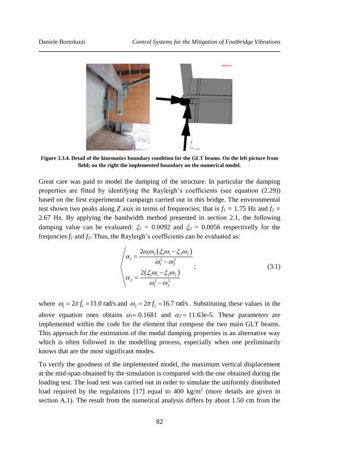
Daniele Bortoluzzi Control Systems for the Mitigation of Footbridge Vibrations
82
Figure 3.3.4. Detail of the kinematics boundary condition for the GLT beams. On the left picture from
field; on the right the implemented boundary on the numerical model.
Great care was paid to model the damping of the structure. In particular the damping
properties are fitted by identifying the Rayleigh’s coefficients (see equation (2.29))
based on the first experimental campaign carried out in this bridge. The environmental
test shown two peaks along Z axis in terms of frequencies; that is f1 = 1.75 Hz and f2 =
2.67 Hz. By applying the bandwidth method presented in section 2.1, the following
damping value can be evaluated: 1 = 0.0092 and 2 = 0.0056 respectivelly for the
frequncies f1 and f2. Thus, the Rayleigh’s coefficients can be evaluated as:
1 2 1 1 2 2
1 2 2
1 2
1 1 2 2
2 2 2
1 2
2
2
; (3.1)
where 1 12 11.0 rad/sf and 2 22 16.7 rad/sf . Substituting these values in the
above equation ones obtains 0.1681 and 11.63e-5. These parameters are
implemented within the code for the element that compose the two main GLT beams.
This approach for the estimation of the modal damping properties is an alternative way
which is often followed in the modelling process, especially when one preliminarily
knows that are the most significant modes.
To verify the goodness of the implemented model, the maximum vertical displacement
at the mid-span obtained by the simulation is compared with the one obtained during the
loading test. The load test was carried out in order to simulate the uniformly distributed
load required by the regulations [17] equal to 400 kg/m2 (more details are given in
section A.1). The result from the numerical analysis differs by about 1.50 cm from the
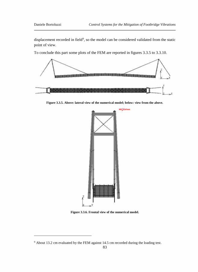
Daniele Bortoluzzi Control Systems for the Mitigation of Footbridge Vibrations
83
displacement recorded in field9, so the model can be considered validated from the static
point of view.
To conclude this part some plots of the FEM are reported in figures 3.3.5 to 3.3.10.
Figure 3.3.5. Above: lateral view of the numerical model; below: view from the above.
Figure 3.3.6. Frontal view of the numerical model.
9 About 13.2 cm evaluated by the FEM against 14.5 cm recorded during the loading test.
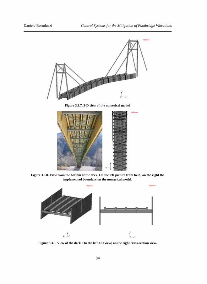
Daniele Bortoluzzi Control Systems for the Mitigation of Footbridge Vibrations
84
Figure 3.3.7. 3-D view of the numerical model.
Figure 3.3.8. View from the bottom of the deck. On the left picture from field; on the right the
implemented boundary on the numerical model.
Figure 3.3.9. View of the deck. On the left 3-D view; on the right cross-section view.
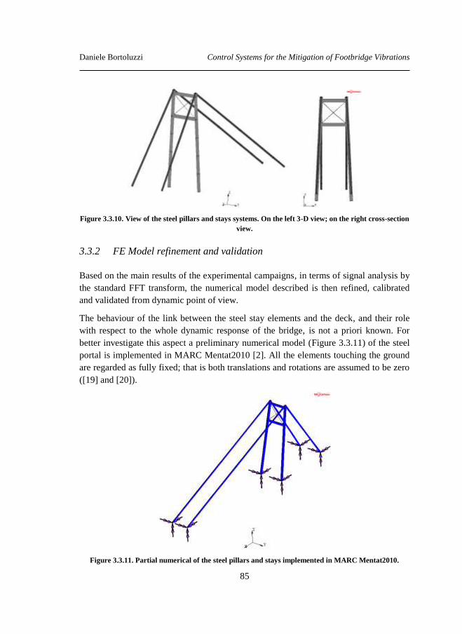
Daniele Bortoluzzi Control Systems for the Mitigation of Footbridge Vibrations
85
Figure 3.3.10. View of the steel pillars and stays systems. On the left 3-D view; on the right cross-section
view.
3.3.2 FE Model refinement and validation
Based on the main results of the experimental campaigns, in terms of signal analysis by
the standard FFT transform, the numerical model described is then refined, calibrated
and validated from dynamic point of view.
The behaviour of the link between the steel stay elements and the deck, and their role
with respect to the whole dynamic response of the bridge, is not a priori known. For
better investigate this aspect a preliminary numerical model (Figure 3.3.11) of the steel
portal is implemented in MARC Mentat2010 [2]. All the elements touching the ground
are regarded as fully fixed; that is both translations and rotations are assumed to be zero
([19] and [20]).
Figure 3.3.11. Partial numerical of the steel pillars and stays implemented in MARC Mentat2010.
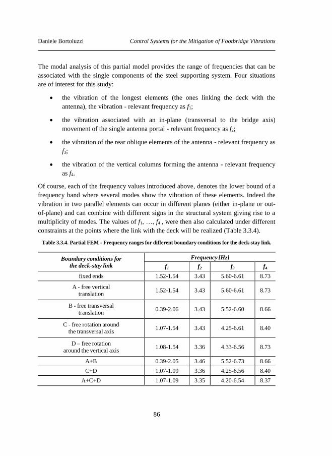
Daniele Bortoluzzi Control Systems for the Mitigation of Footbridge Vibrations
86
The modal analysis of this partial model provides the range of frequencies that can be
associated with the single components of the steel supporting system. Four situations
are of interest for this study:
the vibration of the longest elements (the ones linking the deck with the
antenna), the vibration - relevant frequency as f1;
the vibration associated with an in-plane (transversal to the bridge axis)
movement of the single antenna portal - relevant frequency as f2;
the vibration of the rear oblique elements of the antenna - relevant frequency as
f3;
the vibration of the vertical columns forming the antenna - relevant frequency
as f4.
Of course, each of the frequency values introduced above, denotes the lower bound of a
frequency band where several modes show the vibration of these elements. Indeed the
vibration in two parallel elements can occur in different planes (either in-plane or out-
of-plane) and can combine with different signs in the structural system giving rise to a
multiplicity of modes. The values of f1, …, f4 , were then also calculated under different
constraints at the points where the link with the deck will be realized (Table 3.3.4).
Table 3.3.4. Partial FEM - Frequency ranges for different boundary conditions for the deck-stay link.
Boundary conditions for
the deck-stay link
Frequency [Hz]
f1 f2 f3 f4
fixed ends 1.52-1.54 3.43 5.60-6.61 8.73
A - free vertical
translation 1.52-1.54 3.43 5.60-6.61 8.73
B - free transversal
translation 0.39-2.06 3.43 5.52-6.60 8.66
C - free rotation around
the transversal axis 1.07-1.54 3.43 4.25-6.61 8.40
D – free rotation
around the vertical axis 1.08-1.54 3.36 4.33-6.56 8.73
A+B 0.39-2.05 3.46 5.52-6.73 8.66
C+D 1.07-1.09 3.36 4.25-6.56 8.40
A+C+D 1.07-1.09 3.35 4.20-6.54 8.37
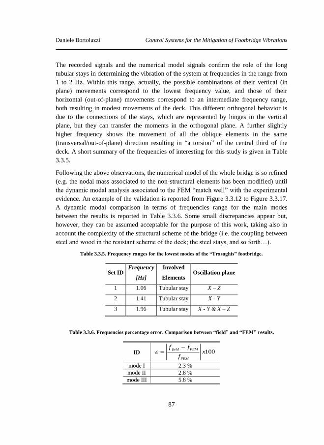
Daniele Bortoluzzi Control Systems for the Mitigation of Footbridge Vibrations
87
The recorded signals and the numerical model signals confirm the role of the long
tubular stays in determining the vibration of the system at frequencies in the range from
1 to 2 Hz. Within this range, actually, the possible combinations of their vertical (in
plane) movements correspond to the lowest frequency value, and those of their
horizontal (out-of-plane) movements correspond to an intermediate frequency range,
both resulting in modest movements of the deck. This different orthogonal behavior is
due to the connections of the stays, which are represented by hinges in the vertical
plane, but they can transfer the moments in the orthogonal plane. A further slightly
higher frequency shows the movement of all the oblique elements in the same
(transversal/out-of-plane) direction resulting in “a torsion” of the central third of the
deck. A short summary of the frequencies of interesting for this study is given in Table
3.3.5.
Following the above observations, the numerical model of the whole bridge is so refined
(e.g. the nodal mass associated to the non-structural elements has been modified) until
the dynamic modal analysis associated to the FEM “match well” with the experimental
evidence. An example of the validation is reported from Figure 3.3.12 to Figure 3.3.17.
A dynamic modal comparison in terms of frequencies range for the main modes
between the results is reported in Table 3.3.6. Some small discrepancies appear but,
however, they can be assumed acceptable for the purpose of this work, taking also in
account the complexity of the structural scheme of the bridge (i.e. the coupling between
steel and wood in the resistant scheme of the deck; the steel stays, and so forth…).
Table 3.3.5. Frequency ranges for the lowest modes of the “Trasaghis” footbridge.
Set ID Frequency
[Hz]
Involved
Elements Oscillation plane
1 1.06 Tubular stay X – Z
2 1.41 Tubular stay X - Y
3 1.96 Tubular stay X - Y & X – Z
Table 3.3.6. Frequencies percentage error. Comparison between “field” and “FEM” results.
ID 100field FEM
FEM
f fx
f
mode I 2.3 %
mode II 2.8 %
mode III 5.8 %
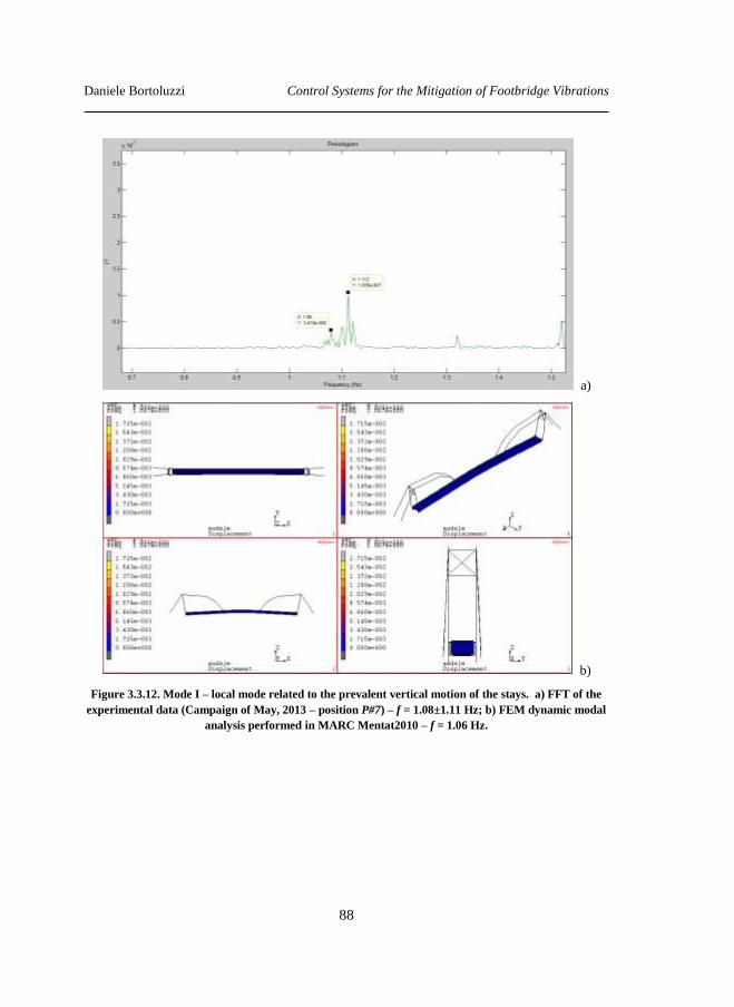
Daniele Bortoluzzi Control Systems for the Mitigation of Footbridge Vibrations
88
a)
b)
Figure 3.3.12. Mode I – local mode related to the prevalent vertical motion of the stays. a) FFT of the
experimental data (Campaign of May, 2013 – position P#7) – f = 1.08±1.11 Hz; b) FEM dynamic modal
analysis performed in MARC Mentat2010 – f = 1.06 Hz.
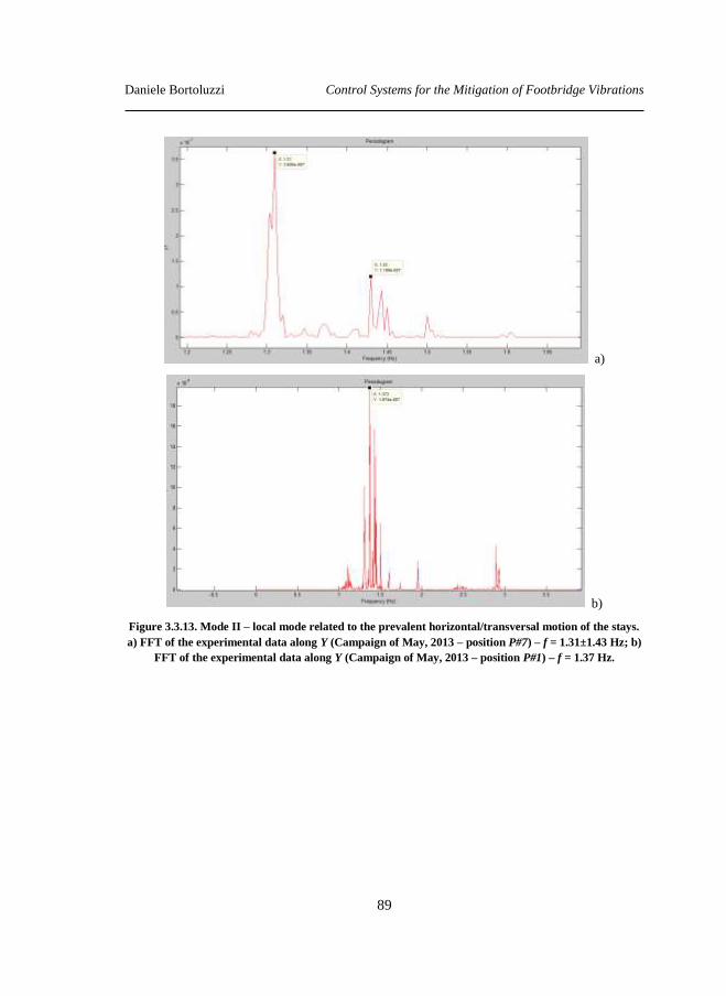
Daniele Bortoluzzi Control Systems for the Mitigation of Footbridge Vibrations
89
a)
b)
Figure 3.3.13. Mode II – local mode related to the prevalent horizontal/transversal motion of the stays.
a) FFT of the experimental data along Y (Campaign of May, 2013 – position P#7) – f = 1.31±1.43 Hz; b)
FFT of the experimental data along Y (Campaign of May, 2013 – position P#1) – f = 1.37 Hz.
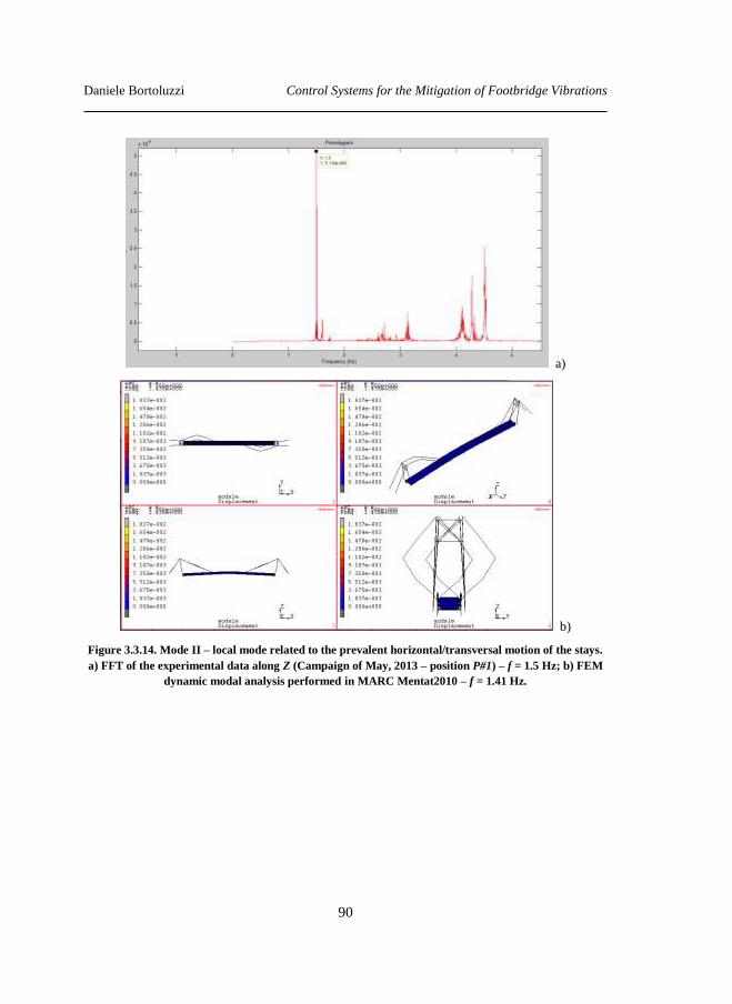
Daniele Bortoluzzi Control Systems for the Mitigation of Footbridge Vibrations
90
a)
b)
Figure 3.3.14. Mode II – local mode related to the prevalent horizontal/transversal motion of the stays.
a) FFT of the experimental data along Z (Campaign of May, 2013 – position P#1) – f = 1.5 Hz; b) FEM
dynamic modal analysis performed in MARC Mentat2010 – f = 1.41 Hz.
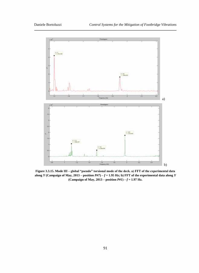
Daniele Bortoluzzi Control Systems for the Mitigation of Footbridge Vibrations
91
a)
b)
Figure 3.3.15. Mode III – global “pseudo” torsional mode of the deck. a) FFT of the experimental data
along Y (Campaign of May, 2013 – position P#7) – f = 1.95 Hz; b) FFT of the experimental data along Y
(Campaign of May, 2013 – position P#1) – f = 1.97 Hz.
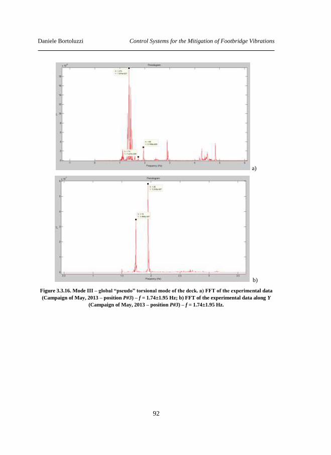
Daniele Bortoluzzi Control Systems for the Mitigation of Footbridge Vibrations
92
a)
b)
Figure 3.3.16. Mode III – global “pseudo” torsional mode of the deck. a) FFT of the experimental data
(Campaign of May, 2013 – position P#3) – f = 1.74±1.95 Hz; b) FFT of the experimental data along Y
(Campaign of May, 2013 – position P#3) – f = 1.74±1.95 Hz.
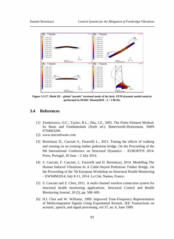
Daniele Bortoluzzi Control Systems for the Mitigation of Footbridge Vibrations
93
Figure 3.3.17. Mode III – global “pseudo” torsional mode of the deck. FEM dynamic modal analysis
performed in MARC Mentat2010 – f = 1.96 Hz.
3.4 References
[1] Zienkiewicz, O.C.; Taylor, R.L.; Zhu, J.Z., 2005. The Finite Element Method:
Its Basis and Fundamentals (Sixth ed.). Butterworth-Heinemann. ISBN
0750663200.
[2] www.mscsoftware.com
[3] Bortoluzzi D., Casciati S., Faravelli L., 2013. Testing the effects of walking
and running on an existing timber pedestrian bridge. On the Proceeding of the
9th International Conference on Structural Dynamics - EURODYN 2014.
Porto, Portugal, 30 June – 2 July 2014.
[4] S. Casciati, F. Casciati, L. Faravelli and D. Bortoluzzi, 2014. Modelling The
Human Induced Vibrations In A Cable-Stayed Pedestrian Timber Bridge. On
the Proceeding of the 7th European Workshop on Structural Health Monitoring
– EWSHM2014, July 8-11, 2014. La Cité, Nantes, France.
[5] S. Casciati and Z. Chen, 2011. A multi‐channel wireless connection system for
structural health monitoring applications. Structural Control and Health
Monitoring Journal, 18 (5), pp. 588–600.
[6] H.I. Choi and W. Williams, 1989. Improved Time-Frequency Representation
of Multicomponent Signals Using Exponential Kernels. IEE Transactions on
acoustic, speech, and signal processing, vol 37, no. 6, June 1989.
Daniele Bortoluzzi Control Systems for the Mitigation of Footbridge Vibrations
94
[7] L. Cohen, 1995. Time-frequency Analysis. Electrical engineering signal
processing Prentice Hall Signal Processing series (1st edition - 1995).
[8] Mallat, S., 1999. A Wavelet Tour of Signal Processing, 2nd edn. London, UK.
Academic Press.
[9] Burrus, C.S., Gopinath, R.A. and Guo, H. Introduction to Wavelets and
Wavelet Transforms, 1st edn, Englewood Cliffs,NJ: Prentice Hall Inc.
[10] B. Peeters and G. De Roeck., 1999. Reference-based stochastic subspace
identification for output-only modal analysis. Mechanical Systems and Signal
Processing, 13(6):855-878. Theory reference for the SSI method available in
MACEC.
[11] E. Reynders and G. De Roeck., 2008. Reference-based combined
deterministic-stochastic subspace identification for experimental and
operational modal analysis. Mechanical Systems and Signal Processing,
22(3):617-637. Theory reference for the CSI method available in MACEC.
[12] E. Reynders, D. Degrauwe, G. De Roeck, F. Magalhães, and E. Caetano.,
2010. Combined experimental-operational modal testing of footbridges. ASCE
Journal of Engineering Mechanics, 136(6):687-696. Two case studies on the
use of OMA and OMAX for footbridge testing, for which MACEC was used.
[13] www.mathworks.it
[14] MACEC a MatLAB toolbox - http://bwk.kuleuven.be/bwm/macec
[15] Bortoluzzi D., Casciati F., Casciati S., Faravelli L., Chen Z., 2013. Reporting
the results of two experimental campaigns on a pedestrian timber bridge - 9th
International Workshop on Structural Health Monitoring 2013 – IWSHM -
Stanford University, Stanford, CA – USA, September 10-2, 2013.
[16] Bortoluzzi D., Casciati F., Casciati S., Faravelli L, 2013. Comparison of
accelerometric response records on a timber footbridge. On the Proceeding of
2nd International Conference on Timber Bridges 2013 – ICTB2013, Las
Vegas, Nevada USA, September-October, 2013.
[17] NTC 2008. Norme tecniche per le costruzioni (in Italian) - D.M. 14 Gennaio
2008.
[18] S. Casciati and M. Domansechi, 2007. Random imperfection fields to model
the size effect in laboratory wood specimens, Structural Safety, 29 (4), pp. 308-
321.
Daniele Bortoluzzi Control Systems for the Mitigation of Footbridge Vibrations
95
[19] Casciati S., Faravelli L. and Bortoluzzi D., 2013. Pedestrian timber bridges:
experimental investigation and modelling. On the Proceeding of the 10th
International Conference on Damage Assessment of Structures - DAMAS 2013.
Trinity College Dublin Ireland, July 8-10 2013.
[20] Casciati S., Faravelli L., Bortoluzzi D., 2013. Human Induced Vibrations In A
Pedestrian Timber Bridge. On the Proceeding of the 4th International
Conference on Computational Methods in Structural Dynamics & Earthquake
Engineering - COMPDYN2013, Kos Island (GR), 12-14 Jun 2013.

Daniele Bortoluzzi Control Systems for the Mitigation of Footbridge Vibrations
96
Daniele Bortoluzzi Control Systems for the Mitigation of Footbridge Vibrations
97
Chapter 4 Modeling the main actions
As already pointed out in Chapter 2, when one works with the design and/or control of
slender structures as pedestrian bridges, generally the main problems are related with
the comfort of the users rather than with the strength of the construction materials. Thus
an inaccurate modelling definition of the load(s) at the design stage could result
dangerous in term of both resistance and comfort.
Thus, one of the main challenges for the designer is to identify the most suitable model
of the live load(s), to be applied on the structure in order to capture/identify the most
reliable response of the structure under study. To achieve this purpose a pure theoretical
defintion of the loads could result unsatisfactory. The best result is achieved merging
theoretical aspects with observations made in laboratory and/or in the field on a real
case study.
An incorrect definition of the live loads during the design stage can be produces two
concatenated effects in terms of comfort; they are:
1) an ineffective performance with, in the worst case, a decrease in the achieved
comfort level;
2) a damage from the economic point of view. In fact, usually, in order to achieve
a better level of comfort one needs to install ad hoc devices on the structure,
i.e. TMDs, dampers and so forth…, that are expensive in term of both
installation and maintenance.
In this chapter, models of the main loads to be considered in the design of pedestrian
bridges are presented ([1] and [2]) for:
1) the wind load;
2) the Human Induced Loads (HIL).
For both of them one is looking for models which allows the simulation of time
histories of random field realizations.
Daniele Bortoluzzi Control Systems for the Mitigation of Footbridge Vibrations
98
For the first one the procedure based on a stochastic simulation approach, comes from
the literature [9] (see section 4.1). For the case of the human induced vibration a new
model for the crowd load is discussed in section 4.2.
4.1 Wind action
In previous chapter, the wind has been introduced as “ambient vibration” (or
background noise) and it has been used for the calibration and validation of the
numerical models of the two footbridges under study. In this section a more
sophisticated mathematical model of the wind is introduced for the purpose of this
thesis: i.e. implementation of different control solutions for the mitigation of the
footbridge vibrations.
In wind engineering, Monte Carlo simulation is becoming one of the most important
tool for the design of wind-excited structures [3]. The following formulas describe the
procedure adopted in this work.
The wind velocity is usually idealized as the sum of two components: the first one, the
“mean” part (U), is assumed to be constant along a given time interval; the second
component, the “fluctuating” part (u), represents the atmospheric turbulence. It is
usually modelled as a stationary zero mean Gaussian random process. To simulate the
fluctuating part the “weighted amplitude waves superposition” (WAWS) method is
adopted in this thesis [4]-[7].
Let 1 2 3;O x x x be the global Cartesian reference system with O lying on the ground, and
the 3x axis parallel to the gravity direction (Figure 4.1.1). One also assumes, without less
of generality, that U is parallel to the 1x axis. Within the above hypotheses one can
write:
3, , ,t x t V x U u x (4.1)
in which,
* 3
3
0
1ln ,
xx u
k z
U along 1x axis, (4.2)
where k=0.41 is the Von Karman constant [4], z0 the roughness length and *u the shear
velocity. An example [8] of the mean wind velocity profile with the height is reported in
for three different scenario of roughness in Figure 4.1.2.
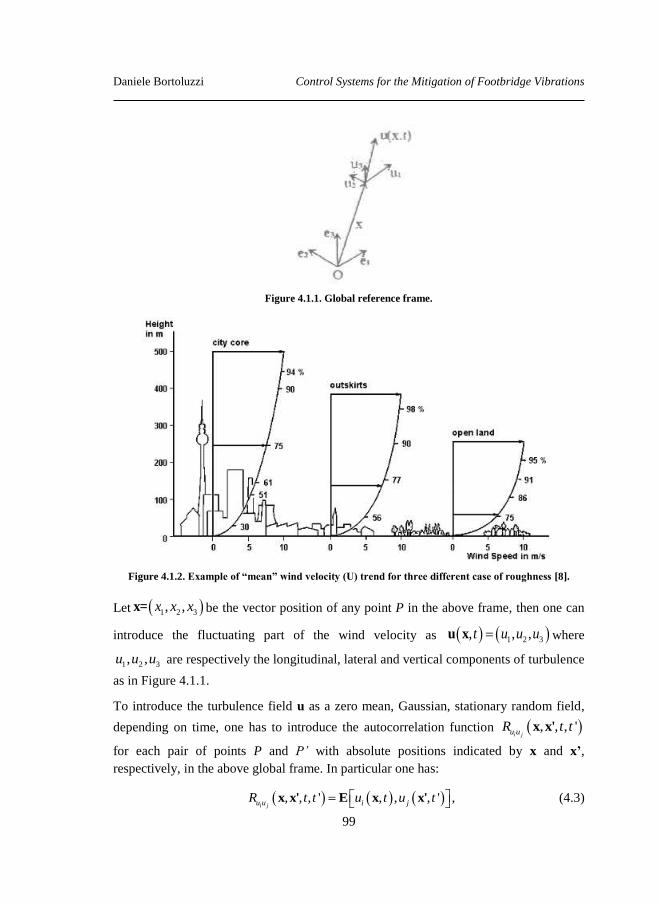
Daniele Bortoluzzi Control Systems for the Mitigation of Footbridge Vibrations
99
Figure 4.1.1. Global reference frame.
Figure 4.1.2. Example of “mean” wind velocity (U) trend for three different case of roughness [8].
Let 1 2 3, ,x x xx= be the vector position of any point P in the above frame, then one can
introduce the fluctuating part of the wind velocity as 1 2 3, , ,t u u uu x where
1 2 3, ,u u u are respectively the longitudinal, lateral and vertical components of turbulence
as in Figure 4.1.1.
To introduce the turbulence field u as a zero mean, Gaussian, stationary random field,
depending on time, one has to introduce the autocorrelation function , , , 'i ju uR t tx x'
for each pair of points P and P’ with absolute positions indicated by x and x’,
respectively, in the above global frame. In particular one has:
, , , ' , , , ' ,x x' E x x'i ju u i jR t t u t u t (4.3)
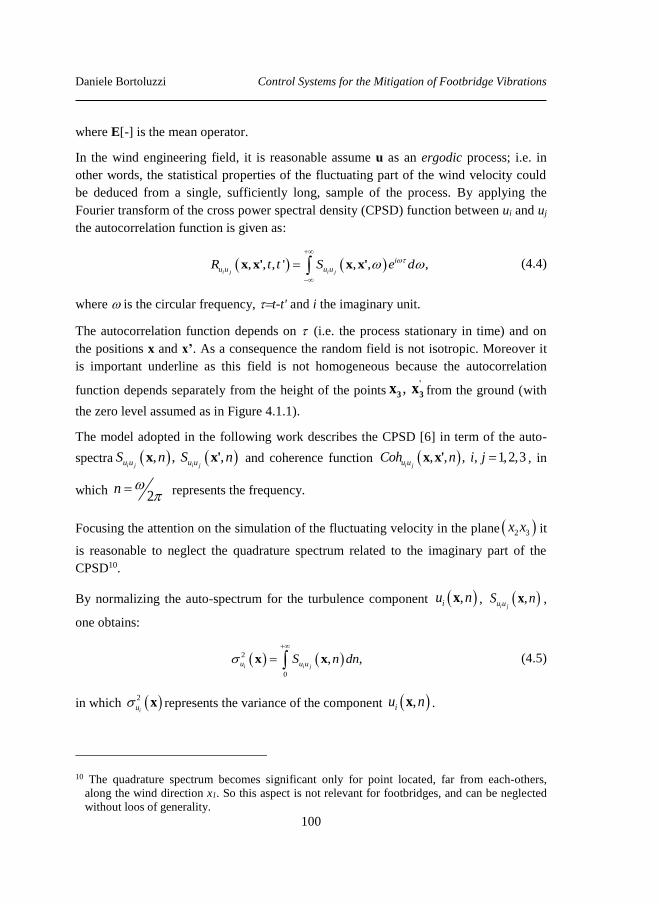
Daniele Bortoluzzi Control Systems for the Mitigation of Footbridge Vibrations
100
where E[-] is the mean operator.
In the wind engineering field, it is reasonable assume u as an ergodic process; i.e. in
other words, the statistical properties of the fluctuating part of the wind velocity could
be deduced from a single, sufficiently long, sample of the process. By applying the
Fourier transform of the cross power spectral density (CPSD) function between ui and uj
the autocorrelation function is given as:
, , , ' , , ,i j i j
i
u u u uR t t S e d
x x' x x' (4.4)
where is the circular frequency, t-t' and i the imaginary unit.
The autocorrelation function depends on (i.e. the process stationary in time) and on
the positions x and x’. As a consequence the random field is not isotropic. Moreover it
is important underline as this field is not homogeneous because the autocorrelation
function depends separately from the height of the points , '
3 3x x from the ground (with
the zero level assumed as in Figure 4.1.1).
The model adopted in the following work describes the CPSD [6] in term of the auto-
spectra , , ,i j i ju u u uS n S nx x' and coherence function , , , , 1,2,3
i ju uCoh n i j x x' , in
which 2n
represents the frequency.
Focusing the attention on the simulation of the fluctuating velocity in the plane 2 3x x it
is reasonable to neglect the quadrature spectrum related to the imaginary part of the
CPSD10.
By normalizing the auto-spectrum for the turbulence component ,iu nx , ,i ju uS nx ,
one obtains:
2
0
, ,i i ju u uS n dn
x x (4.5)
in which 2
iu x represents the variance of the component ,iu nx .
10 The quadrature spectrum becomes significant only for point located, far from each-others,
along the wind direction x1. So this aspect is not relevant for footbridges, and can be neglected
without loos of generality.

Daniele Bortoluzzi Control Systems for the Mitigation of Footbridge Vibrations
101
Following the model proposed in [9] and [10] the auto-spectrum ,i ju uS nx of the three
components of the turbulence can be analytically given as:
2 53
,, 1,2,3 ,
1 1.5
ii j
i
i
j uu u
uj u
n LnS nj
n L
x U xx
xx U x
(4.6)
where iuL is the integral length scale of the turbulence component ju , and
1 2 36.868, 9.434, 6.103 .
The three components of the turbulence 1 2 3, , ,t u u uu x , that are orthogonal to each
other, are usually assumed statistically uncorrelated. Vice versa, the dependency of each
pairs of parallel turbulence components in two distinct points of the space is described
by the coherence function modelled as follows:
2 2 2' ' '
1 1 1 2 2 2 3 3 3
, ,
2 2 2exp , 1,2,3 ,
i ju u
j j j
Coh n
n C x x C x x C x xj
x xx x'
U x U x'
(4.7)
where the coefficient Cjs represents the exponential decay of the component uj versus the
longitudinal (s=1), lateral (s=2) and vertical (s=3) displacements respectively.
Once introduced the problem from a mathematical point of view, in order to obtain a
simulated realization of the wind velocity field, one needs to discretize the spatial
domain into k=1,2,3,…,N nodes which usually represent some significant points of the
structure under study11. Assuming that 1 2 3, ,k k k k
x x xx = represent the position of the
generic k-th node of the discretized space, (4.1) can be rewritten simply as:
, , , 1,2,3,...,k k kk kt t t k N V V x U x u x , (4.8)
where 1 2 3, ,k k ku u u are, once again, respectively the longitudinal, lateral and vertical
components of turbulence in the k-th node of the simulation domain. Following the
11 Usually the same points corresponds to a subset of the nodes used in the numerical model
(FEM).

Daniele Bortoluzzi Control Systems for the Mitigation of Footbridge Vibrations
102
above approach the time-dependent turbulence random field 1 2 3, , ,t u u uu x , is
transformed into a 3N-variate stationary random process tu , where tu is a 3N-
order vector containing the components 1 2 3, ,
k k ku u u of the turbulence vector
ktu .
The characterization of the tu process is complete introducing the power spectral
density matrix (PSD) of order N x N defined as:
1 1 1
1
,
N
N N N
u u u u
u u u u
S n S n
S n
S n S n
uu (4.9)
where each component are defined by a matrix of order 3 x 3:
1 1 1 2 1 3
2 1 2 2 2 3
3 1 2 3 33
, , 1,2,...,
h k h k h k
h k h k h k h k
h k h k h k
u u u u u u
u u u u u u u u
u u u u u u
S n S n S n
S n S n S n S n h k N
S n S n S n
(4.10)
The PSD in (4.9) is real12, symmetric and positive definite at each frequency value n.
Introduce the two-side power spectral density matrix (2-DPSD) as follows:
1
2,
1
2
S n
G n
S n
uu
uu
uu
(4.11)
where the operator * indicates the complex conjugate.
Since tu is 3N-variate stationary random Gaussian process, it is possible to apply the
Priestley spectral approach to generate its representation; that is:
,i tt e d
u Z (4.12)
12 The PSD is real because the quadrature spectrum has been neglected.
Daniele Bortoluzzi Control Systems for the Mitigation of Footbridge Vibrations
103
where Z is a zero-mean normal complex random process in which
d d Z Z Z that satisfies:
*
0
''
0
uu
E Z
E Z Z
T
d
G d ifd d
otherwise
(4.13)
Moreover, since the simulated process is a real-value process the Hermitian symmetry is
guaranteed; that is *d d Z Z .
Introducing now the vector w containing 3N complex-value uncorrelated white
noise with unit variance and Hermetian symmetry, and an ad hoc deterministic matrix
*|T
G uuT T T , it is possible to rewrite the increment d Z as
follows:
d d Z T w . (4.14)
Substituting (4.14) into (4.12) it is possible to rewrite the random process tu as:
,i tt e d
u T w (4.15)
It is convenient to apply the decomposition of the 2-DPSD matrix by the Cholesky
factorization13:
11
21 22
3 1 3 2 3 3
0 ... 0
... 0,
...N N N N
T
T T
T T T
T (4.16)
The discrete version of the equation (4.15) can be written as:
,ki t
k kt e
u T w (4.17)
13 This approach is not unique. Different factorization/decomposition can be applied.
Daniele Bortoluzzi Control Systems for the Mitigation of Footbridge Vibrations
104
where the following sequence of uniformly spaced circular frequencies k with step
is considered:
2
1 1,..., 12
,
2,...,2
k
N k
Nk for k
Nfor k N
(4.18)
in which a cut-off circular frequency 2
c
N
is introduced.
Introducing the decomposition proposed in (4.16) into equation (4.17), the j-th
component of the process can be rewritten as:
1 1
, 1,2,...,3k
ji t
j jr k r k
r k
u t e T w j N
(4.19)
and it can be used for the simulation process by truncating the summation to the finite
number N of harmonics. The entire simulation of the process tu is then generated
along a sequence of tN uniformly spaced time instant defined as:
1 , 1,..., .j tt j t for j N (4.20)
Equation (4.19) might be interpreted as a multidimensional Fourier series in which the
fundamental circular frequency is represented by , and the corresponding period is
defined as 2 .PT The simulation represented in (4.19) may be interpreted as a
process with periodicity .PT Therefore, the simulation of the process requires to be
satisfied the following condition about its time duration:
.sample Pt T (4.21)
More in general, must be satisfied the following conditions:
2
4
t
c
N t
t
(4.22)
An alternative representation of the equation (4.19) is given in [5]; that is:
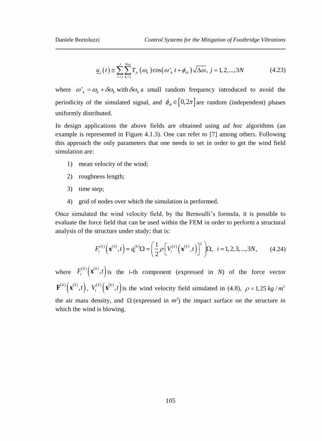
Daniele Bortoluzzi Control Systems for the Mitigation of Footbridge Vibrations
105
1 1
cos ' , 1,2,...,3j N
j jr k k rk
r k
u t T t j N
(4.23)
where 'k k k with k a small random frequency introduced to avoid the
periodicity of the simulated signal, and 0,2rk are random (independent) phases
uniformly distributed.
In design applications the above fields are obtained using ad hoc algorithms (an
example is represented in Figure 4.1.3). One can refer to [7] among others. Following
this approach the only parameters that one needs to set in order to get the wind field
simulation are:
1) mean velocity of the wind;
2) roughness length;
3) time step;
4) grid of nodes over which the simulation is performed.
Once simulated the wind velocity field, by the Bernoulli’s formula, it is possible to
evaluate the force field that can be used within the FEM in order to perform a structural
analysis of the structure under study; that is:
21
, , , 1,2,3,...,3 ,2
k k k k k
i i iF t q V t i N
x x (4.24)
where ,xk k
iF t is the i-th component (expressed in N) of the force vector
,F xk k
t , ,xk k
iV t is the wind velocity field simulated in (4.8), 31,25 / kg m
the air mass density, and (expressed in m2) the impact surface on the structure in
which the wind is blowing.
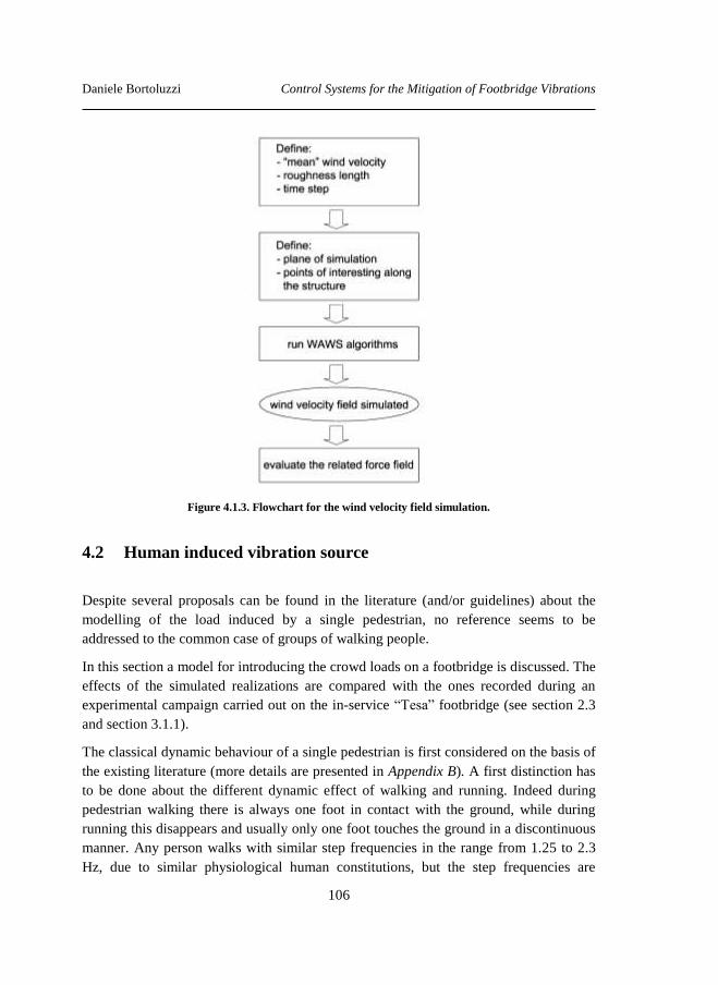
Daniele Bortoluzzi Control Systems for the Mitigation of Footbridge Vibrations
106
Figure 4.1.3. Flowchart for the wind velocity field simulation.
4.2 Human induced vibration source
Despite several proposals can be found in the literature (and/or guidelines) about the
modelling of the load induced by a single pedestrian, no reference seems to be
addressed to the common case of groups of walking people.
In this section a model for introducing the crowd loads on a footbridge is discussed. The
effects of the simulated realizations are compared with the ones recorded during an
experimental campaign carried out on the in-service “Tesa” footbridge (see section 2.3
and section 3.1.1).
The classical dynamic behaviour of a single pedestrian is first considered on the basis of
the existing literature (more details are presented in Appendix B). A first distinction has
to be done about the different dynamic effect of walking and running. Indeed during
pedestrian walking there is always one foot in contact with the ground, while during
running this disappears and usually only one foot touches the ground in a discontinuous
manner. Any person walks with similar step frequencies in the range from 1.25 to 2.3
Hz, due to similar physiological human constitutions, but the step frequencies are
Daniele Bortoluzzi Control Systems for the Mitigation of Footbridge Vibrations
107
influenced by the purpose of the movement and the intensity of the pedestrian loading
[11].
The most common time domain models for these forces scheme can be found in
literature and/or in the guidelines (see [11]-[14] among others). They are based on the
assumption that both human feet produce the same force. The resulting periodic force is
expressed by standard Fourier series as follows:
vertical (gravity) component:
,
1
( ) 1 sin(2 )k
v n v v n
n
F t P nf t
; (4.25)
lateral (transversal) component:
,lat
1
( ) sin(2 )k
lat n lat n
n
F t P nf t
; (4.26)
The model of the pedestrian running is more complicated because, during the run, there
is a so called “lift-off phase”, during which no foot is in contact with the ground. Only
the vertical component of these forces is taken into consideration because it has been
observed as the horizontal components, both lateral and longitudinal, have a low
“impact” on the dynamic response of the bridge [14]. The vertical component is
modelled by using the standard Fourier transform as follows:
,
1
,
1( ) sin(2 ) for 1
2
1( ) 0 for
2
k
r vert n r m m
n
r vert m m
F t P P nf t j T t j T
F t j T t jT
; (4.27)
4.2.1 Crowd Load Model (CLM)
In order to simulate the interaction between the structure and the human induced loads
in a realistic manner, a model for the load due to a group of persons is required. In this
section a numerical model of the crowd load is discussed. As already observed in
section 2.3, the proposed model is validated on the base of the records acquired during
the experimental campaign carried out on the “Tesa” footbridge.
A numerical model for the crowd load has to be account for several aspects:
psychology, motion, individual feeling and so forth… The introduction of the global
effects of these aspects by an amplification factor, as suggested in some guidelines (e.g.
[14]), could result quite inaccurate.
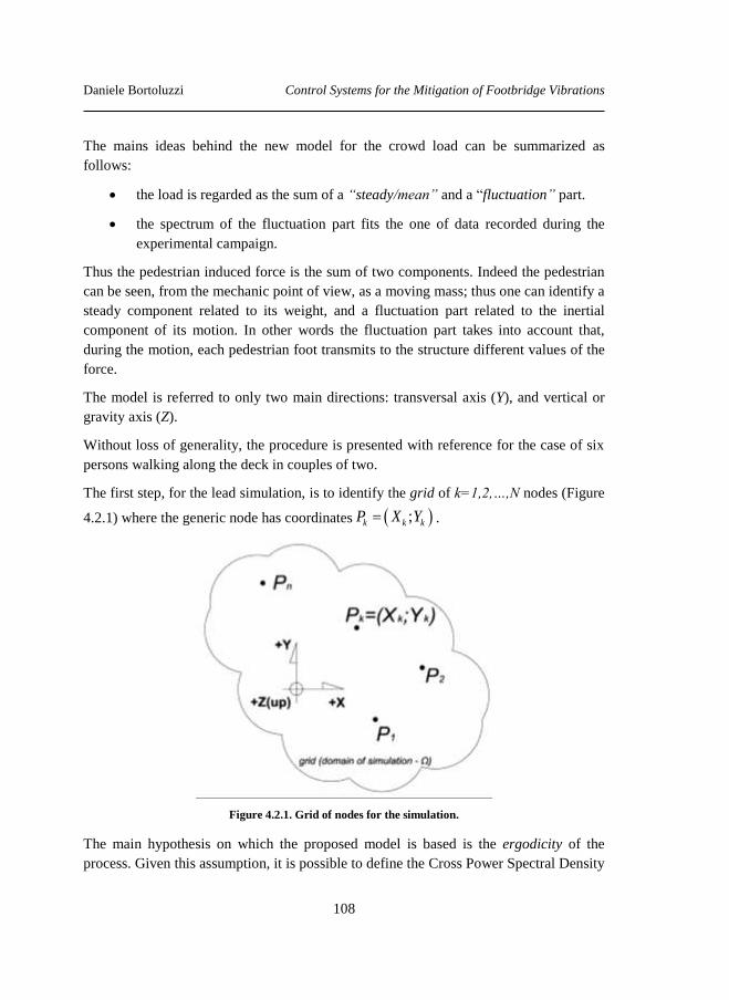
Daniele Bortoluzzi Control Systems for the Mitigation of Footbridge Vibrations
108
The mains ideas behind the new model for the crowd load can be summarized as
follows:
the load is regarded as the sum of a “steady/mean” and a “fluctuation” part.
the spectrum of the fluctuation part fits the one of data recorded during the
experimental campaign.
Thus the pedestrian induced force is the sum of two components. Indeed the pedestrian
can be seen, from the mechanic point of view, as a moving mass; thus one can identify a
steady component related to its weight, and a fluctuation part related to the inertial
component of its motion. In other words the fluctuation part takes into account that,
during the motion, each pedestrian foot transmits to the structure different values of the
force.
The model is referred to only two main directions: transversal axis (Y), and vertical or
gravity axis (Z).
Without loss of generality, the procedure is presented with reference for the case of six
persons walking along the deck in couples of two.
The first step, for the lead simulation, is to identify the grid of k=1,2,…,N nodes (Figure
4.2.1) where the generic node has coordinates ;k k kP X Y .
Figure 4.2.1. Grid of nodes for the simulation.
The main hypothesis on which the proposed model is based is the ergodicity of the
process. Given this assumption, it is possible to define the Cross Power Spectral Density
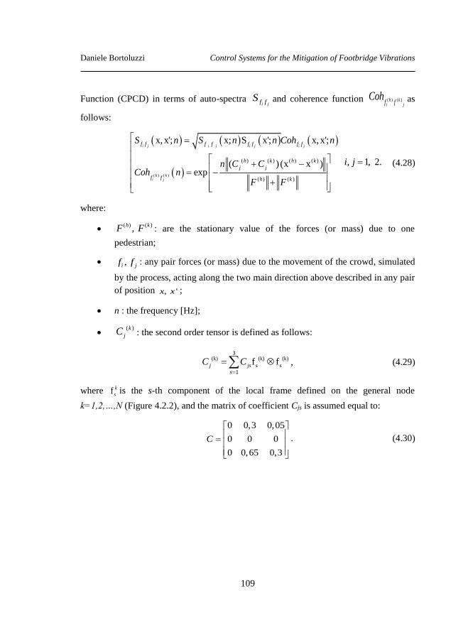
Daniele Bortoluzzi Control Systems for the Mitigation of Footbridge Vibrations
109
Function (CPCD) in terms of auto-spectra i jf fS and coherence function ( ) ( )h k
i jf fCoh as
follows:
( )( )
( ) ( ) ( ) ( )
( ) ( )
x, x'; x; S x'; x, x';
, 1, 2.( ) (x x )exp
i j i j i j i j
khi j
f f f f f f f f
h k h k
j j
f f h k
S n S n n Coh n
i jn C CCoh n
F F
(4.28)
where:
( ) ( ), h kF F : are the stationary value of the forces (or mass) due to one
pedestrian;
, i jf f : any pair forces (or mass) due to the movement of the crowd, simulated
by the process, acting along the two main direction above described in any pair
of position , 'x x ;
n : the frequency [Hz];
( )k
jC : the second order tensor is defined as follows:
(k) (k) (k)f fj js s s
s
C C
3
1
, (4.29)
where f k
sis the s-th component of the local frame defined on the general node
k=1,2,…,N (Figure 4.2.2), and the matrix of coefficient Cjs is assumed equal to:
0 0,3 0,05
0 0 0
0 0,65 0,3
C
. (4.30)
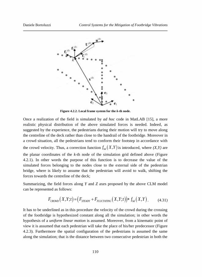
Daniele Bortoluzzi Control Systems for the Mitigation of Footbridge Vibrations
110
Figure 4.2.2. Local frame system for the k-th node.
Once a realization of the field is simulated by ad hoc code in MatLAB [15], a more
realistic physical distribution of the above simulated forces is needed. Indeed, as
suggested by the experience, the pedestrians during their motion will try to move along
the centreline of the deck rather than close to the handrail of the footbridge. Moreover in
a crowd situation, all the pedestrians tend to conform their footstep in accordance with
the crowd velocity. Thus, a correction function ,bdf X Y is introduced, where (X,Y) are
the planar coordinates of the k-th node of the simulation grid defined above (Figure
4.2.1). In other words the purpose of this function is to decrease the value of the
simulated forces belonging to the nodes close to the external side of the pedestrian
bridge, where is likely to assume that the pedestrian will avoid to walk, shifting the
forces towards the centreline of the deck;
Summarizing, the field forces along Y and Z axes proposed by the above CLM model
can be represented as follows:
, ; , ; ,CROWD STEADY FLUCTATING bdF X Y t F F X Y t f X Y . (4.31)
It has to be underlined as in this procedure the velocity of the crowd during the crossing
of the footbridge is hypothesized constant along all the simulation; in other words the
hypothesis of a uniform linear motion is assumed. Moreover, from a kinematic point of
view it is assumed that each pedestrian will take the place of his/her predecessor (Figure
4.2.3). Furthermore the spatial configuration of the pedestrians is assumed the same
along the simulation; that is the distance between two consecutive pedestrian in both the
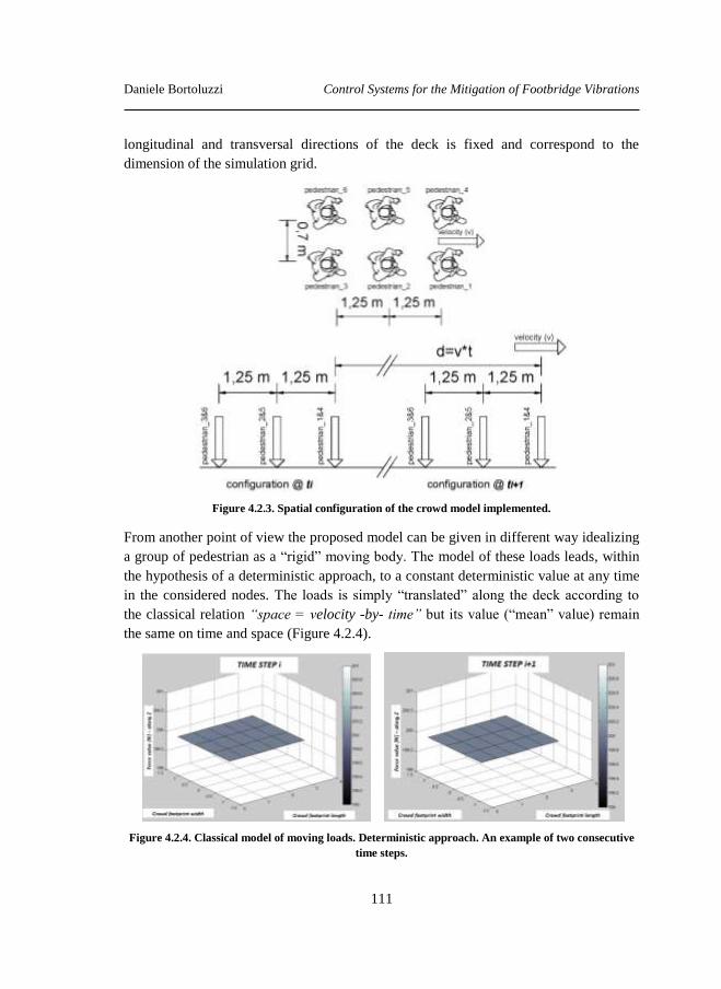
Daniele Bortoluzzi Control Systems for the Mitigation of Footbridge Vibrations
111
longitudinal and transversal directions of the deck is fixed and correspond to the
dimension of the simulation grid.
Figure 4.2.3. Spatial configuration of the crowd model implemented.
From another point of view the proposed model can be given in different way idealizing
a group of pedestrian as a “rigid” moving body. The model of these loads leads, within
the hypothesis of a deterministic approach, to a constant deterministic value at any time
in the considered nodes. The loads is simply “translated” along the deck according to
the classical relation “space = velocity -by- time” but its value (“mean” value) remain
the same on time and space (Figure 4.2.4).
Figure 4.2.4. Classical model of moving loads. Deterministic approach. An example of two consecutive
time steps.
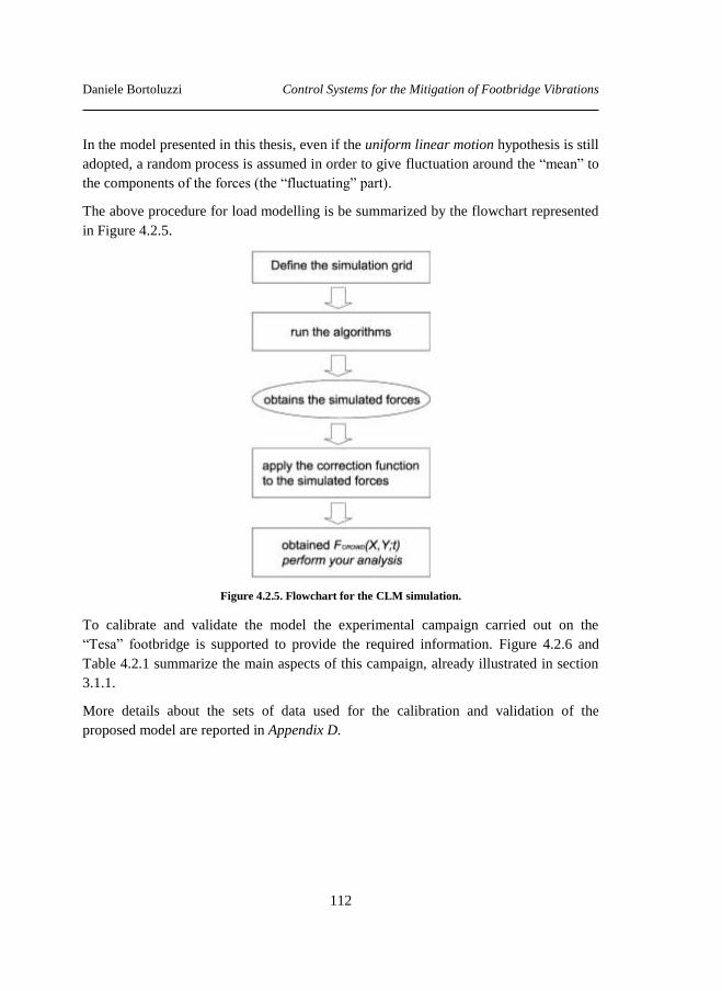
Daniele Bortoluzzi Control Systems for the Mitigation of Footbridge Vibrations
112
In the model presented in this thesis, even if the uniform linear motion hypothesis is still
adopted, a random process is assumed in order to give fluctuation around the “mean” to
the components of the forces (the “fluctuating” part).
The above procedure for load modelling is be summarized by the flowchart represented
in Figure 4.2.5.
Figure 4.2.5. Flowchart for the CLM simulation.
To calibrate and validate the model the experimental campaign carried out on the
“Tesa” footbridge is supported to provide the required information. Figure 4.2.6 and
Table 4.2.1 summarize the main aspects of this campaign, already illustrated in section
3.1.1.
More details about the sets of data used for the calibration and validation of the
proposed model are reported in Appendix D.
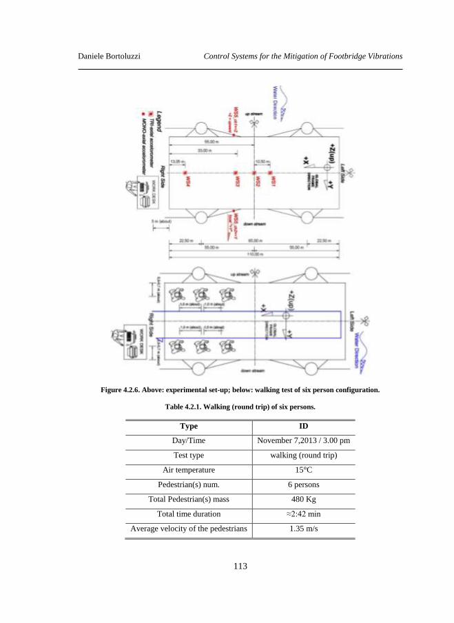
Daniele Bortoluzzi Control Systems for the Mitigation of Footbridge Vibrations
113
Figure 4.2.6. Above: experimental set-up; below: walking test of six person configuration.
Table 4.2.1. Walking (round trip) of six persons.
Type ID
Day/Time November 7,2013 / 3.00 pm
Test type walking (round trip)
Air temperature 15°C
Pedestrian(s) num. 6 persons
Total Pedestrian(s) mass 480 Kg
Total time duration ≈2:42 min
Average velocity of the pedestrians 1.35 m/s
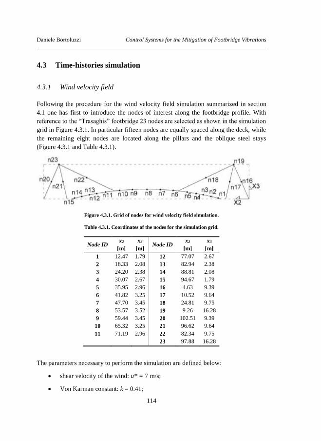
Daniele Bortoluzzi Control Systems for the Mitigation of Footbridge Vibrations
114
4.3 Time-histories simulation
4.3.1 Wind velocity field
Following the procedure for the wind velocity field simulation summarized in section
4.1 one has first to introduce the nodes of interest along the footbridge profile. With
reference to the “Trasaghis” footbridge 23 nodes are selected as shown in the simulation
grid in Figure 4.3.1. In particular fifteen nodes are equally spaced along the deck, while
the remaining eight nodes are located along the pillars and the oblique steel stays
(Figure 4.3.1 and Table 4.3.1).
Figure 4.3.1. Grid of nodes for wind velocity field simulation.
Table 4.3.1. Coordinates of the nodes for the simulation grid.
Node ID x2
[m]
x3
[m] Node ID
x2
[m]
x3
[m]
1 12.47 1.79 12 77.07 2.67
2 18.33 2.08 13 82.94 2.38
3 24.20 2.38 14 88.81 2.08
4 30.07 2.67 15 94.67 1.79
5 35.95 2.96 16 4.63 9.39
6 41.82 3.25 17 10.52 9.64
7 47.70 3.45 18 24.81 9.75
8 53.57 3.52 19 9.26 16.28
9 59.44 3.45 20 102.51 9.39
10 65.32 3.25 21 96.62 9.64
11 71.19 2.96 22 82.34 9.75
23 97.88 16.28
The parameters necessary to perform the simulation are defined below:
shear velocity of the wind: u* = 7 m/s;
Von Karman constant: k = 0.41;
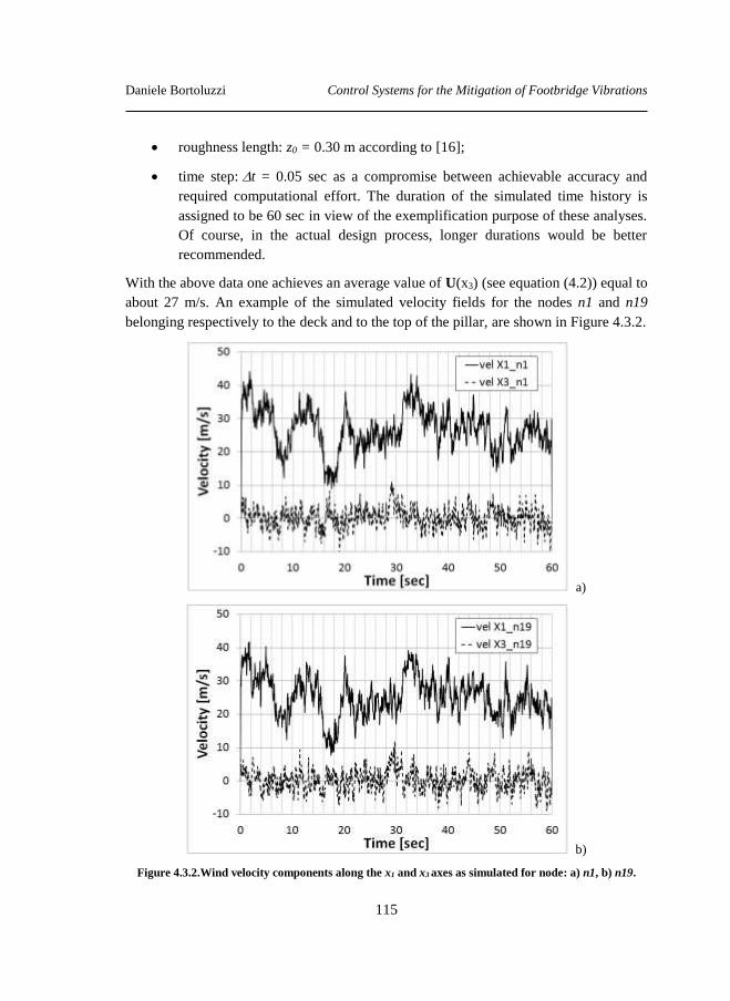
Daniele Bortoluzzi Control Systems for the Mitigation of Footbridge Vibrations
115
roughness length: z0 = 0.30 m according to [16];
time step:t = 0.05 sec as a compromise between achievable accuracy and
required computational effort. The duration of the simulated time history is
assigned to be 60 sec in view of the exemplification purpose of these analyses.
Of course, in the actual design process, longer durations would be better
recommended.
With the above data one achieves an average value of U(x3) (see equation (4.2)) equal to
about 27 m/s. An example of the simulated velocity fields for the nodes n1 and n19
belonging respectively to the deck and to the top of the pillar, are shown in Figure 4.3.2.
a)
b)
Figure 4.3.2.Wind velocity components along the x1 and x3 axes as simulated for node: a) n1, b) n19.

Daniele Bortoluzzi Control Systems for the Mitigation of Footbridge Vibrations
116
Once the wind velocity field is obtained, by applying the equation (4.24), the related
force field for each node of the grid is calculated. When introducing the time histories as
boundary conditions in the finite element analyses, one can either consider them as
instantaneously applied (with consequent impact phenomena that can be create several
problems during the dynamic analysis), or “smooth” them by applying an initial and a
final linear ramp (to avoid the above impact phenomena). The second option is then
adopted. As an example in Figure 4.3.3 the time histories of the forces for the nodes n8,
n22 and n23 are plotted. For each node the two components along the x1 and x3 axes are
plotted.
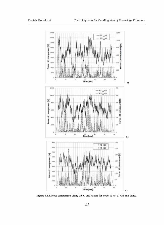
Daniele Bortoluzzi Control Systems for the Mitigation of Footbridge Vibrations
117
a)
b)
c)
Figure 4.3.3.Force components along the x1 and x3 axes for node: a) n8, b) n22 and c) n23.
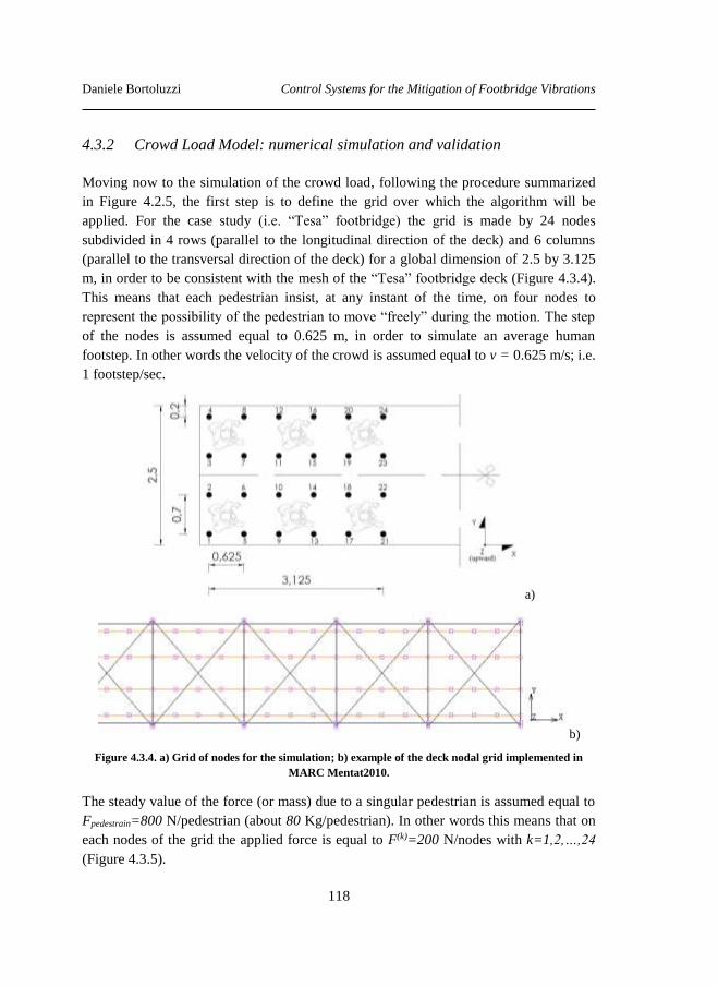
Daniele Bortoluzzi Control Systems for the Mitigation of Footbridge Vibrations
118
4.3.2 Crowd Load Model: numerical simulation and validation
Moving now to the simulation of the crowd load, following the procedure summarized
in Figure 4.2.5, the first step is to define the grid over which the algorithm will be
applied. For the case study (i.e. “Tesa” footbridge) the grid is made by 24 nodes
subdivided in 4 rows (parallel to the longitudinal direction of the deck) and 6 columns
(parallel to the transversal direction of the deck) for a global dimension of 2.5 by 3.125
m, in order to be consistent with the mesh of the “Tesa” footbridge deck (Figure 4.3.4).
This means that each pedestrian insist, at any instant of the time, on four nodes to
represent the possibility of the pedestrian to move “freely” during the motion. The step
of the nodes is assumed equal to 0.625 m, in order to simulate an average human
footstep. In other words the velocity of the crowd is assumed equal to v = 0.625 m/s; i.e.
1 footstep/sec.
a)
b)
Figure 4.3.4. a) Grid of nodes for the simulation; b) example of the deck nodal grid implemented in
MARC Mentat2010.
The steady value of the force (or mass) due to a singular pedestrian is assumed equal to
Fpedestrain=800 N/pedestrian (about 80 Kg/pedestrian). In other words this means that on
each nodes of the grid the applied force is equal to F(k)=200 N/nodes with k=1,2,…,24
(Figure 4.3.5).
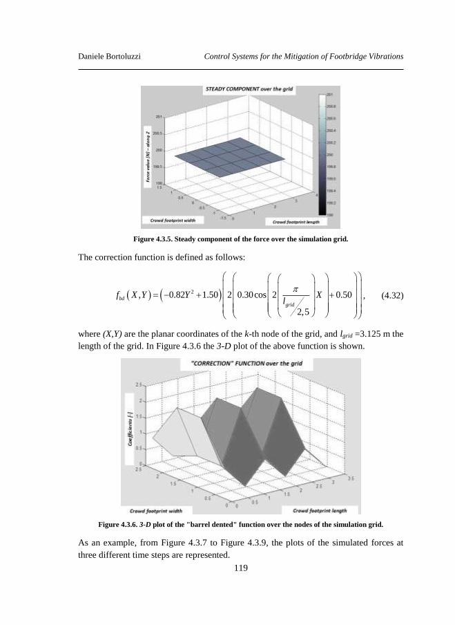
Daniele Bortoluzzi Control Systems for the Mitigation of Footbridge Vibrations
119
Figure 4.3.5. Steady component of the force over the simulation grid.
The correction function is defined as follows:
2, 0.82 1.50 2 0.30cos 2 0.50
2,5
bd
grid
f X Y Y Xl
, (4.32)
where (X,Y) are the planar coordinates of the k-th node of the grid, and lgrid =3.125 m the
length of the grid. In Figure 4.3.6 the 3-D plot of the above function is shown.
Figure 4.3.6. 3-D plot of the "barrel dented" function over the nodes of the simulation grid.
As an example, from Figure 4.3.7 to Figure 4.3.9, the plots of the simulated forces at
three different time steps are represented.
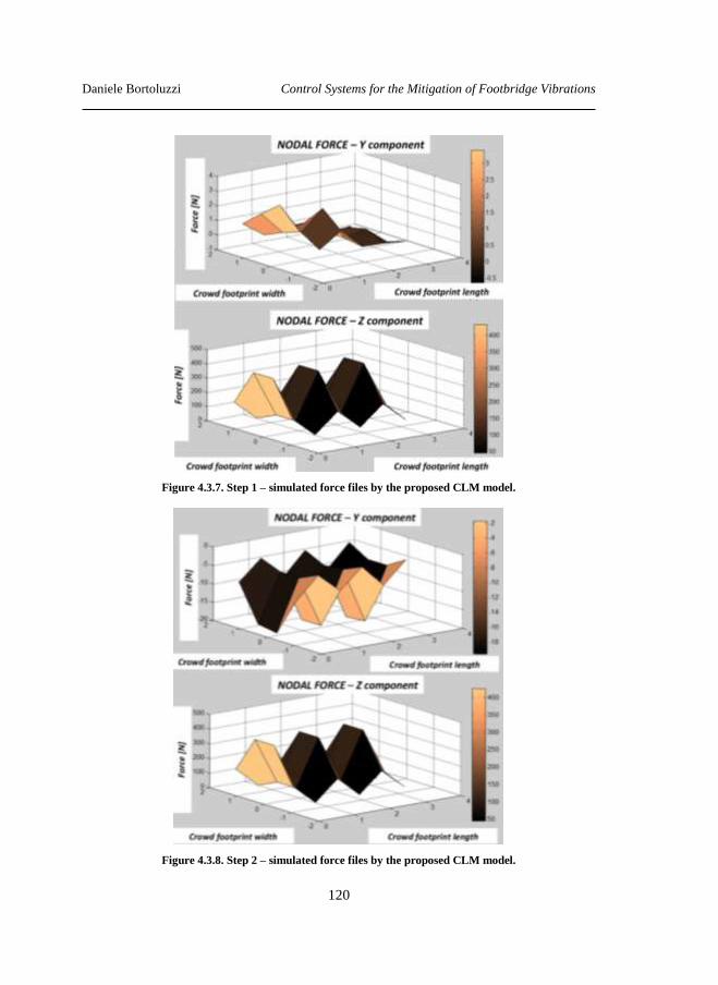
Daniele Bortoluzzi Control Systems for the Mitigation of Footbridge Vibrations
120
Figure 4.3.7. Step 1 – simulated force files by the proposed CLM model.
Figure 4.3.8. Step 2 – simulated force files by the proposed CLM model.
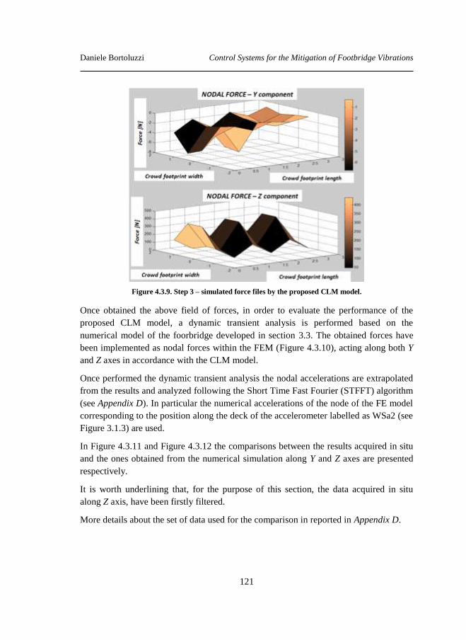
Daniele Bortoluzzi Control Systems for the Mitigation of Footbridge Vibrations
121
Figure 4.3.9. Step 3 – simulated force files by the proposed CLM model.
Once obtained the above field of forces, in order to evaluate the performance of the
proposed CLM model, a dynamic transient analysis is performed based on the
numerical model of the foorbridge developed in section 3.3. The obtained forces have
been implemented as nodal forces within the FEM (Figure 4.3.10), acting along both Y
and Z axes in accordance with the CLM model.
Once performed the dynamic transient analysis the nodal accelerations are extrapolated
from the results and analyzed following the Short Time Fast Fourier (STFFT) algorithm
(see Appendix D). In particular the numerical accelerations of the node of the FE model
corresponding to the position along the deck of the accelerometer labelled as WSa2 (see
Figure 3.1.3) are used.
In Figure 4.3.11 and Figure 4.3.12 the comparisons between the results acquired in situ
and the ones obtained from the numerical simulation along Y and Z axes are presented
respectively.
It is worth underlining that, for the purpose of this section, the data acquired in situ
along Z axis, have been firstly filtered.
More details about the set of data used for the comparison in reported in Appendix D.
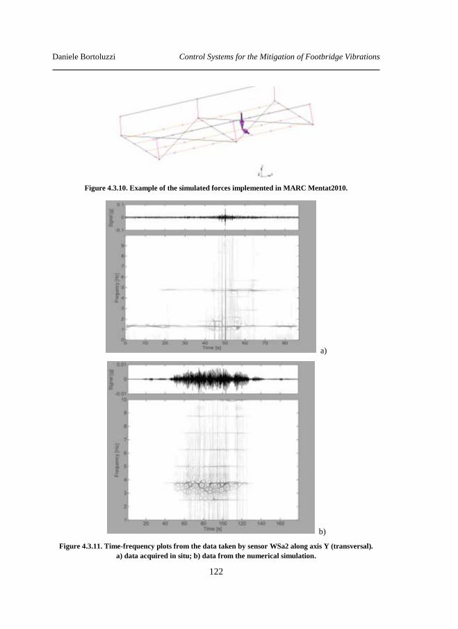
Daniele Bortoluzzi Control Systems for the Mitigation of Footbridge Vibrations
122
Figure 4.3.10. Example of the simulated forces implemented in MARC Mentat2010.
a)
b)
Figure 4.3.11. Time-frequency plots from the data taken by sensor WSa2 along axis Y (transversal).
a) data acquired in situ; b) data from the numerical simulation.
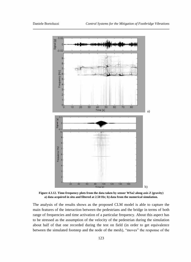
Daniele Bortoluzzi Control Systems for the Mitigation of Footbridge Vibrations
123
a)
b)
Figure 4.3.12. Time-frequency plots from the data taken by sensor WSa2 along axis Z (gravity)
a) data acquired in situ and filtered at 2.50 Hz; b) data from the numerical simulation.
The analysis of the results shows as the proposed CLM model is able to capture the
main features of the interaction between the pedestrians and the bridge in terms of both
range of frequencies and time activation of a particular frequency. About this aspect has
to be stressed as the assumption of the velocity of the pedestrian during the simulation
about half of that one recorded during the test on field (in order to get equivalence
between the simulated footstep and the node of the mesh), “moves” the response of the
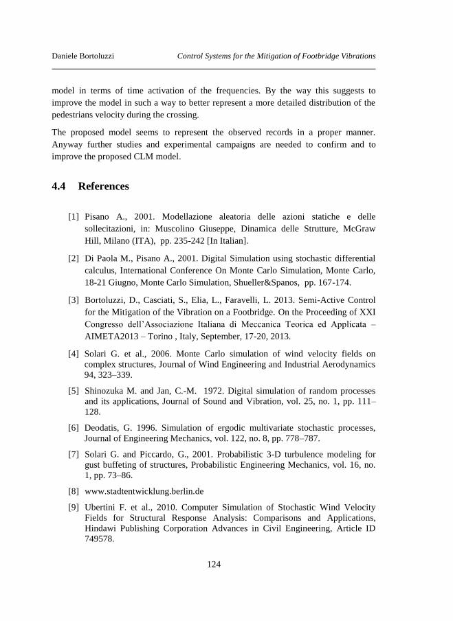
Daniele Bortoluzzi Control Systems for the Mitigation of Footbridge Vibrations
124
model in terms of time activation of the frequencies. By the way this suggests to
improve the model in such a way to better represent a more detailed distribution of the
pedestrians velocity during the crossing.
The proposed model seems to represent the observed records in a proper manner.
Anyway further studies and experimental campaigns are needed to confirm and to
improve the proposed CLM model.
4.4 References
[1] Pisano A., 2001. Modellazione aleatoria delle azioni statiche e delle
sollecitazioni, in: Muscolino Giuseppe, Dinamica delle Strutture, McGraw
Hill, Milano (ITA), pp. 235-242 [In Italian].
[2] Di Paola M., Pisano A., 2001. Digital Simulation using stochastic differential
calculus, International Conference On Monte Carlo Simulation, Monte Carlo,
18-21 Giugno, Monte Carlo Simulation, Shueller&Spanos, pp. 167-174.
[3] Bortoluzzi, D., Casciati, S., Elia, L., Faravelli, L. 2013. Semi-Active Control
for the Mitigation of the Vibration on a Footbridge. On the Proceeding of XXI
Congresso dell’Associazione Italiana di Meccanica Teorica ed Applicata –
AIMETA2013 – Torino , Italy, September, 17-20, 2013.
[4] Solari G. et al., 2006. Monte Carlo simulation of wind velocity fields on
complex structures, Journal of Wind Engineering and Industrial Aerodynamics
94, 323–339.
[5] Shinozuka M. and Jan, C.-M. 1972. Digital simulation of random processes
and its applications, Journal of Sound and Vibration, vol. 25, no. 1, pp. 111–
128.
[6] Deodatis, G. 1996. Simulation of ergodic multivariate stochastic processes,
Journal of Engineering Mechanics, vol. 122, no. 8, pp. 778–787.
[7] Solari G. and Piccardo, G., 2001. Probabilistic 3-D turbulence modeling for
gust buffeting of structures, Probabilistic Engineering Mechanics, vol. 16, no.
1, pp. 73–86.
[8] www.stadtentwicklung.berlin.de
[9] Ubertini F. et al., 2010. Computer Simulation of Stochastic Wind Velocity
Fields for Structural Response Analysis: Comparisons and Applications,
Hindawi Publishing Corporation Advances in Civil Engineering, Article ID
749578.
Daniele Bortoluzzi Control Systems for the Mitigation of Footbridge Vibrations
125
[10] G. Solari, G. Piccardo, 2001. Probabilistic 3D turbulence modeling for gust
buffeting of structures, Prob. Eng. Mech. (16) pp. 73–86.
[11] Guidelines for the design of footbridges. Fib bulletin 32, November 2005.
[12] Heinemeyer, C., Butz, C., Keil, A., Mark, S., Goldack, A., Trometer, S., Lukić,
M., Chabrolin, B., Lemaire, A., Martin, P., Cunha, Á., Caetano, E., 2009.
Design of Lightweight Footbridges for Human Induced Vibrations.
Background document in support to the implementation, harmonization and
further development of the Eurocodes, JRC European Commission,
Luxembourg.
[13] Živanović, S. et al., 2005. Vibration serviceability of footbridges under human
induced excitation: a literature review. Journal of Sound and Vibration 279, pp.
1-79.
[14] Footbridges: assessment of vibrational behaviour of footbridges under
pedestrian loading - Technical guide, 2006 – Sétra-AFGC.
[15] www.mathworks.it
[16] NTC 2008. Norme tecniche per le costruzioni (in Italian) - D.M. 14 Gennaio
2008.

Daniele Bortoluzzi Control Systems for the Mitigation of Footbridge Vibrations
126
Daniele Bortoluzzi Control Systems for the Mitigation of Footbridge Vibrations
127
Chapter 5 Model order reduction (MOR)
Numerical simulations are nowadays in almost all fields of the sciences an important
tool to predict the behaviour of the process under study by-passing the direct
experimentation on large scale (i.e. laboratory test, field campaign, and so forth…)
which are usually quite expensive.
Accurate simulations imply that the errors of the virtual models be small, and that
different aspects of the process taken into account.
Although the calculation power is greatly improved over the last decades, in the field of
structural engineering, many time one needs to work with dynamic models that may
contain a large number of equations. This makes the analysis heavy in terms of
calculation time. For this reason one needs to simplify these models in order to achieve
lighter models of analysis, by preserving a good approximation of the final results. This
means that if one wants to simplify a given problem it has to be sure to represent all the
main features of the original problem in order to avoid losses of important information.
The Model Order Reduction (MOR) is the label by which such a problem is denoted.
The fundamental methods in the area of Model Order Reduction were published in the
eighties and nineties of the last century. In 1981 Moore [1] published the method of
Truncated Balanced Realization, in 1984 Glover published his famous paper on the
Hankel-norm reduction [2], that are still nowadays the “foundations” of this method.
More details will be given in the followings, but in Figure 5.1 the working concept of
MOR is introduced in a graphical manner. From this figure it is easy-to-understand how
sometimes very little information is required to describe a model. This simple example
shown as, even with only a few facets, the rabbit on the right can still be recognized as
such.
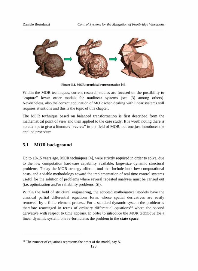
Daniele Bortoluzzi Control Systems for the Mitigation of Footbridge Vibrations
128
Figure 5.1. MOR: graphical representation [4].
Within the MOR techniques, current research studies are focused on the possibility to
“capture” lower order models for nonlinear systems (see [3] among others).
Nevertheless, also the correct application of MOR when dealing with linear systems still
requires attentions and this is the topic of this chapter.
The MOR technique based on balanced transformation is first described from the
mathematical point of view and then applied to the case study. It is worth noting there is
no attempt to give a literature “review” in the field of MOR, but one just introduces the
applied procedure.
5.1 MOR background
Up to 10-15 years ago, MOR techniques [4], were strictly required in order to solve, due
to the low computation hardware capability available, large-size dynamic structural
problems. Today the MOR strategy offers a tool that include both low computational
costs, and a viable methodology toward the implementation of real time control systems
useful for the solution of problems where several repeated analyses must be carried out
(i.e. optimization and/or reliability problems [5]).
Within the field of structural engineering, the adopted mathematical models have the
classical partial differential equations form, whose spatial derivatives are easily
removed, by a finite element process. For a standard dynamic system the problem is
therefore rearranged in terms of ordinary differential equations14 where the second
derivative with respect to time appears. In order to introduce the MOR technique for a
linear dynamic system, one re-formulates the problem in the state space:
14 The number of equations represents the order of the model, say N.
Daniele Bortoluzzi Control Systems for the Mitigation of Footbridge Vibrations
129
d tt t
dt
xAx Bu (5.1)
t t t y Cx Du (5.2)
where u is the input vector, related so to an external excitations (size p), x is the vector
state variables15 of size n and y the response vector of size q, Moreover A is a square
matrix of size n by n, B a matrix of size n by p, C a matrix of size q by n and D a matrix
of size q by p.
Assuming now that the response of the system depends only on the state of the system,
it is possible to neglect the matrix D. Introducing the transformation
| qxnt x t z T T where T is an invertible matrix but not necessarily the unit
matrix, and taking into mind once said above, one has16:
1 z TAT z TBu (5.3)
1y CT z (5.4)
where, as usual, the superposed dot denotes time derivative.
The following steps regard the concepts of reachability and controllability.
A given system is completely reachable if it is possible to determine an ad hoc input
signal able to lead, within a finite time interval, the system from the zero state to a
predefined state. In other words the reachability represents the measure in which the
state of the system can be manipulated by the input u(t). This concept regards only the
state equations [6], so the matrix C and D can be neglected. From a mathematical point
of view one introduces the matrix of reachability QR as:
2 1... .T
n
R
Q B AB A B A B (5.5)
The system is defined as fully reachable if Rrank nQ .
In a similar way a given system is controllable if for each possible initial state of the
system is possible to introduce an ad hoc input signal leads the system to the zero state
in a finite time interval.
15 The state variables are not supposed to have any physical meaning; they have only
mathematical quantities. 16 The dependence over the time is suppressed for sake of simplification.
Daniele Bortoluzzi Control Systems for the Mitigation of Footbridge Vibrations
130
The matrix of observability of the system can be defined as:
2 1...C .
Tn
O
Q C CA CA A (5.6)
The system is then defined as fully observable if Orank nQ .
The next step is to introduce the concept of Gramian [4]. The Gramians are matrices
that contain information about the proprieties of the system, let it to be W:
2
1
t
T
t
d W = G G . (5.7)
In the matrix G the columns represent each single response signal due to the generic
input signal. It is possible to demonstrate that the above matrix W is positive semi-
definite with eigenvalues 2 2 2
1 2 0n and the corresponding eigenvectors
1 2, , , nv v v mutually orthogonal forming a base of orthonormal vectors. Following [1]
it is possible to re-write the matrix of the generic Gramian as:
2
1
2
t
T T
t
d ΛW = G G V V , (5.8)
where 1 2, , , nv v vV is the matrix of eigenvectors, and Λ the diagonal matrix.
Then introduces the following quantities [1]:
0
TA T A
C d
W = e BB e , (5.9)
0
TA T A
O d
W = e CC e , (5.10)
respectively the Gramian matrix of controllability and observability. These matrices
satisfy the air of Lyapunov equations [6]-[10]:
0 T T
C CAW W A BB , (5.11)
0 T T
O OA W AW C C . (5.12)
Finally the balanced transformation to perform the reduction is achieved by:

Daniele Bortoluzzi Control Systems for the Mitigation of Footbridge Vibrations
131
1. solving the Lyapunov equations (5.11) and (5.12) find the Gramian matrices of
controllability (5.9) and observability (5.10);
2. perform the Cholesky factorizations of the Gramian matrices:
T
C C
T
O O
C
O
W L L
W L L. (5.13)
3. evaluate the Singular Values Decomposition (SVD) of the Cholesky factors:
ΛT T
O C L L U V . (5.14)
where U is the matrix of the eigenvectors of the matrix in the r.h.s., say Q, by
its transpose, V is the matrix of the eigenvectors of QTQ and is the diagonal
matrix of the singular values.
4. introduce the balanced transformation [6]:
1 2
1 1 2
Λ
Λ
C
T T
O
T = L V
T = U L. (5.15)
such that 1 ΛT T
C O
T W T T W T = .Evaluate the space of the balanced matrix
as:
1 1 2 1 2
1 1 2
1 2
Λ Λ
Λ
Λ
T T
b O C
T T
b O
b C
T T
T
T
A A = U L AL V
B B = U L B
C C CL V
. (5.16)
To operate a model reduction the Hankel singular values are then introduced.
A given system is considered as fully balanced within the time interval [0,T] if:
2Λ C O
W W , (5.17)
where:
1
22
0 0
0Λ
0
0 0 n
h
h
h
C OW W , (5.18)

Daniele Bortoluzzi Control Systems for the Mitigation of Footbridge Vibrations
132
is a diagonal matrix in which 1 2 0nh h h are the Hankel’s singular values.
Following [7]-[9] these values can be evaluated by:
1 ih C O
W W . (5.19)
Concluding and generalizing the problem, let’s consider a generic balanced model
described by the matrices , , b b bA B C and bD with the corresponding Hankel’s singular
values sorted in descending order. Choose an appropriate truncation r such that hr is
strictly greater than hr+1 and define the state vector 1 2,x x x where x1 corresponds to
the first r component, while x2 the remaining n-r components.
A visual representation of the above MOR technique is given in Figure 5.1.1 [11].
Figure 5.1.1. MOR: visual representation [11].
The concept behind this reduction technique is that the singular values of the
corresponding Hankel matrix tend to the second order modes λi. Because the number of
non-zero singular values of the Hankel matrix determines the order of the system, the
reduction consists in neglecting the λk+1 smaller than a fixed value λk; This operation is
called truncation.
The balance of the system, instead, is the core of the optimization for the order
reduction because the reduced model must retain the properties of controllability and
observability. Thanks to the balancing the values are arranged in descending order that
give a measure of the controllability and observability of the model. Once balanced, one
can proceed with the truncation of the states size in order to exclude the smallest
Hankel’s singular values to achieve the approximate lower model order.

Daniele Bortoluzzi Control Systems for the Mitigation of Footbridge Vibrations
133
This truncation technique is called balanced truncation and consists in the reduction of
the model for elimination of the system’s vibration modes less significant. By
neglecting the smallest Hankel’s values, in other words, one deletes the states that, with
difficulty, will be reached and observed by the system.
If are pushed too much the reductions, or if one decides to ignore a large number of λ,
there is the risk of losing important information about the model (i.e. the structure under
study) analyzed. The result is that the response of the system does not correspond to the
results calculated by an exact solution of the model. For this reason it is important make
a right decision about the appropriate value of λ from where to truncate the model
without compromising the goodness of the final results.
5.2 Structural response
In this section the procedure described in the previous section is applied to the
“Trasaghis” footbridge. In order to apply the MOR to the case study a “lighter”
numerical model compared with the “full” one described in section 3.2.2, is developed
within the MARC Mentat2010 environment [12]. Only beam elements are employed as
reported in Figure 5.2.1. Also for this model great care is taken for the implementation
of the so called non-structural mass as described in section 3.2.2 (e.g. larch cladding,
handrail and so forth…) and for the kinematic boundary condition in order to achieve
the best representation.
The new model is characterized by 301 beam elements and 208 nodes, and it is able to
represent, for the dynamic point of view, the full FEM. A dynamic modal comparison
between the “full” and the “light” FEM of the “Trasaghis” footbridge is reported from
Figure 5.2.2 to Figure 5.2.6. Some discrepancies appear in terms of frequencies as
reported in Table 5.2.1. They could have been reduced by a suitable refinement but this
is out from the exemplification nature of the computational reported.
Figure 5.2.1. “Light” FEM implemented in MARC Mentat2010 environment.
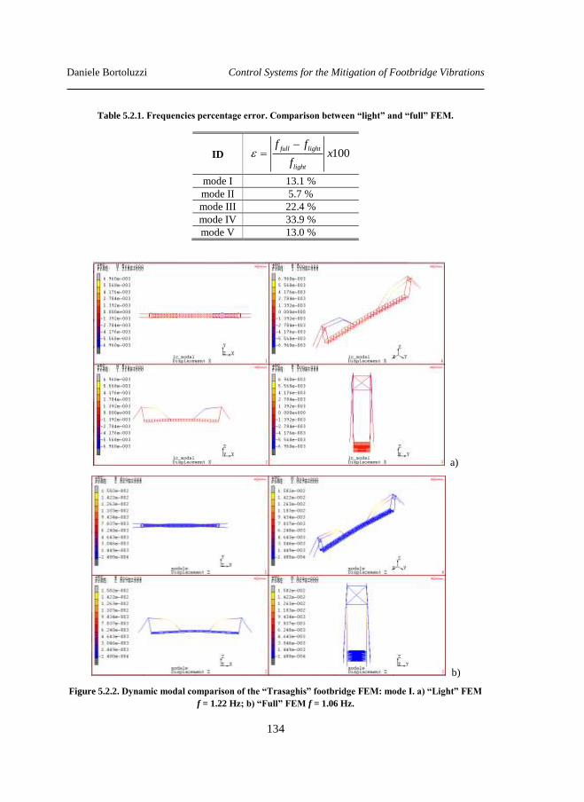
Daniele Bortoluzzi Control Systems for the Mitigation of Footbridge Vibrations
134
Table 5.2.1. Frequencies percentage error. Comparison between “light” and “full” FEM.
ID 100full light
light
f fx
f
mode I 13.1 %
mode II 5.7 %
mode III 22.4 %
mode IV 33.9 %
mode V 13.0 %
a)
b)
Figure 5.2.2. Dynamic modal comparison of the “Trasaghis” footbridge FEM: mode I. a) “Light” FEM
f = 1.22 Hz; b) “Full” FEM f = 1.06 Hz.
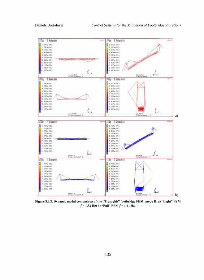
Daniele Bortoluzzi Control Systems for the Mitigation of Footbridge Vibrations
135
a)
b)
Figure 5.2.3. Dynamic modal comparison of the “Trasaghis” footbridge FEM: mode II. a) “Light” FEM
f = 1.32 Hz; b) “Full” FEM f = 1.41 Hz.
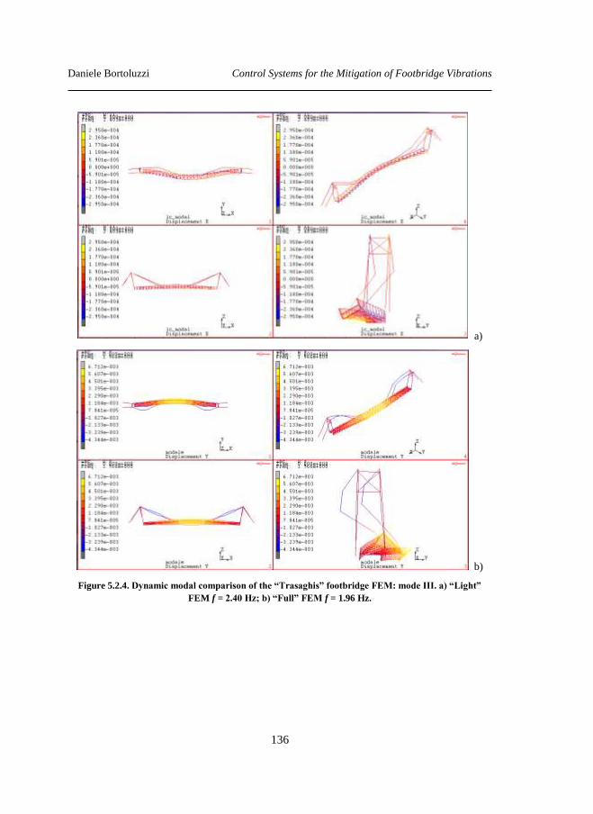
Daniele Bortoluzzi Control Systems for the Mitigation of Footbridge Vibrations
136
a)
b)
Figure 5.2.4. Dynamic modal comparison of the “Trasaghis” footbridge FEM: mode III. a) “Light”
FEM f = 2.40 Hz; b) “Full” FEM f = 1.96 Hz.
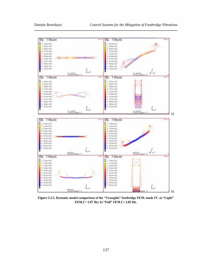
Daniele Bortoluzzi Control Systems for the Mitigation of Footbridge Vibrations
137
a)
b)
Figure 5.2.5. Dynamic modal comparison of the “Trasaghis” footbridge FEM: mode IV. a) “Light”
FEM f = 1.87 Hz; b) “Full” FEM f = 2.83 Hz.
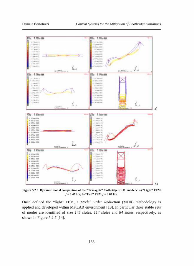
Daniele Bortoluzzi Control Systems for the Mitigation of Footbridge Vibrations
138
a)
b)
Figure 5.2.6. Dynamic modal comparison of the “Trasaghis” footbridge FEM: mode V. a) “Light” FEM
f = 3.47 Hz; b) “Full” FEM f = 3.07 Hz.
Once defined the “light” FEM, a Model Order Reduction (MOR) methodology is
applied and developed within MatLAB environment [13]. In particular three stable sets
of modes are identified of size 145 states, 114 states and 84 states, respectively, as
shown in Figure 5.2.7 [14].
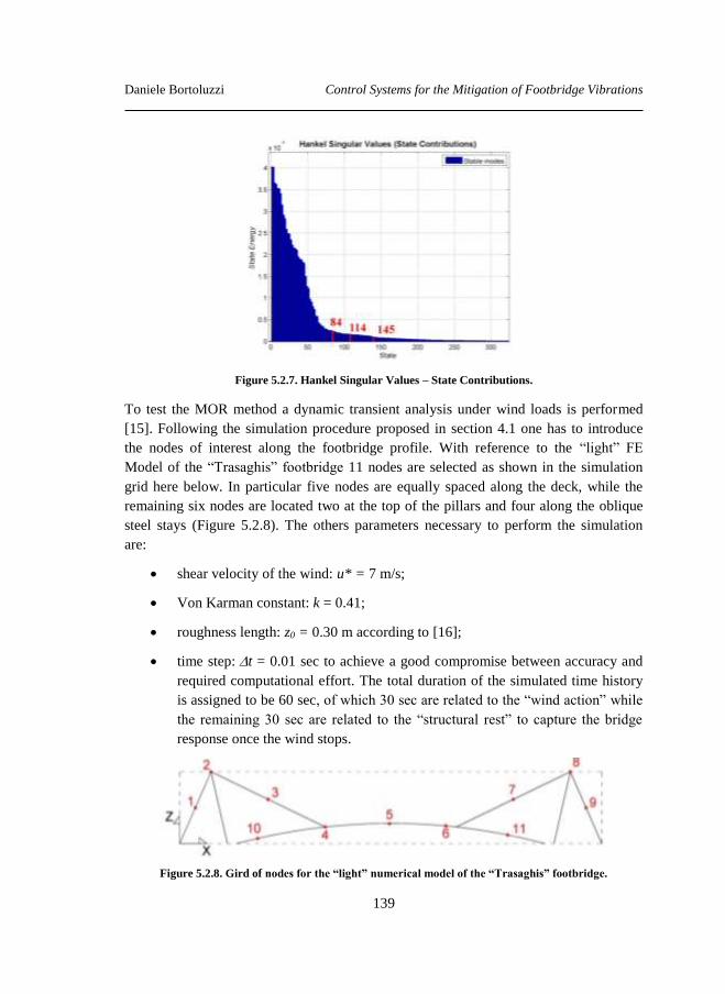
Daniele Bortoluzzi Control Systems for the Mitigation of Footbridge Vibrations
139
Figure 5.2.7. Hankel Singular Values – State Contributions.
To test the MOR method a dynamic transient analysis under wind loads is performed
[15]. Following the simulation procedure proposed in section 4.1 one has to introduce
the nodes of interest along the footbridge profile. With reference to the “light” FE
Model of the “Trasaghis” footbridge 11 nodes are selected as shown in the simulation
grid here below. In particular five nodes are equally spaced along the deck, while the
remaining six nodes are located two at the top of the pillars and four along the oblique
steel stays (Figure 5.2.8). The others parameters necessary to perform the simulation
are:
shear velocity of the wind: u* = 7 m/s;
Von Karman constant: k = 0.41;
roughness length: z0 = 0.30 m according to [16];
time step:t = 0.01 sec to achieve a good compromise between accuracy and
required computational effort. The total duration of the simulated time history
is assigned to be 60 sec, of which 30 sec are related to the “wind action” while
the remaining 30 sec are related to the “structural rest” to capture the bridge
response once the wind stops.
Figure 5.2.8. Gird of nodes for the “light” numerical model of the “Trasaghis” footbridge.
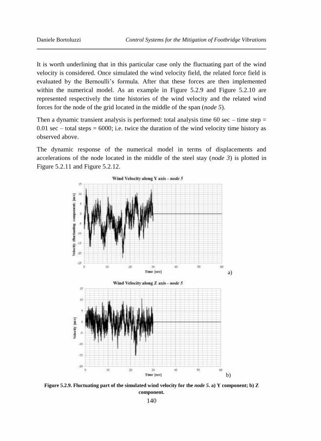
Daniele Bortoluzzi Control Systems for the Mitigation of Footbridge Vibrations
140
It is worth underlining that in this particular case only the fluctuating part of the wind
velocity is considered. Once simulated the wind velocity field, the related force field is
evaluated by the Bernoulli’s formula. After that these forces are then implemented
within the numerical model. As an example in Figure 5.2.9 and Figure 5.2.10 are
represented respectively the time histories of the wind velocity and the related wind
forces for the node of the grid located in the middle of the span (node 5).
Then a dynamic transient analysis is performed: total analysis time 60 sec – time step =
0.01 sec – total steps = 6000; i.e. twice the duration of the wind velocity time history as
observed above.
The dynamic response of the numerical model in terms of displacements and
accelerations of the node located in the middle of the steel stay (node 3) is plotted in
Figure 5.2.11 and Figure 5.2.12.
a)
b)
Figure 5.2.9. Fluctuating part of the simulated wind velocity for the node 5. a) Y component; b) Z
component.
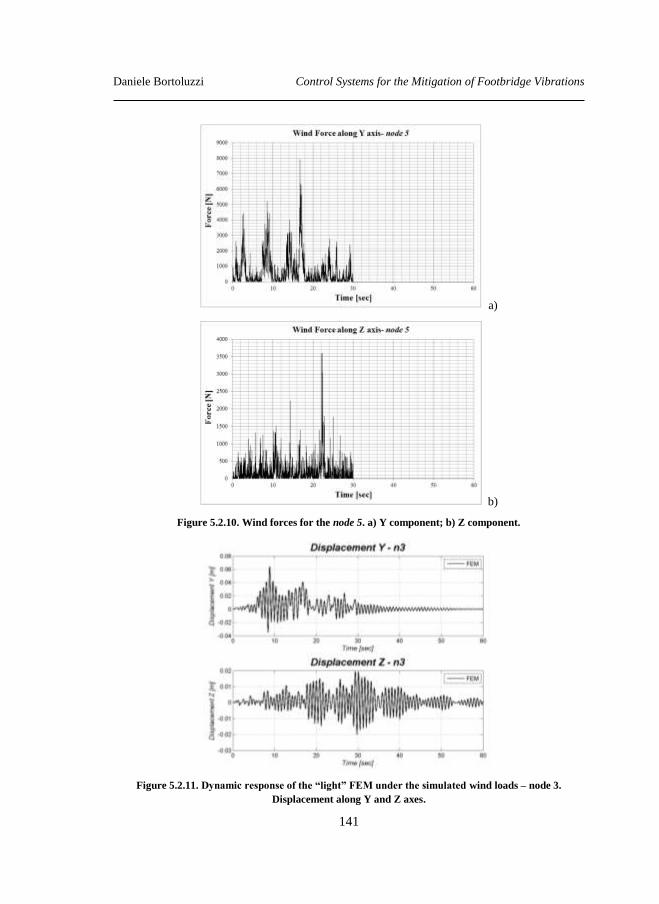
Daniele Bortoluzzi Control Systems for the Mitigation of Footbridge Vibrations
141
a)
b)
Figure 5.2.10. Wind forces for the node 5. a) Y component; b) Z component.
Figure 5.2.11. Dynamic response of the “light” FEM under the simulated wind loads – node 3.
Displacement along Y and Z axes.
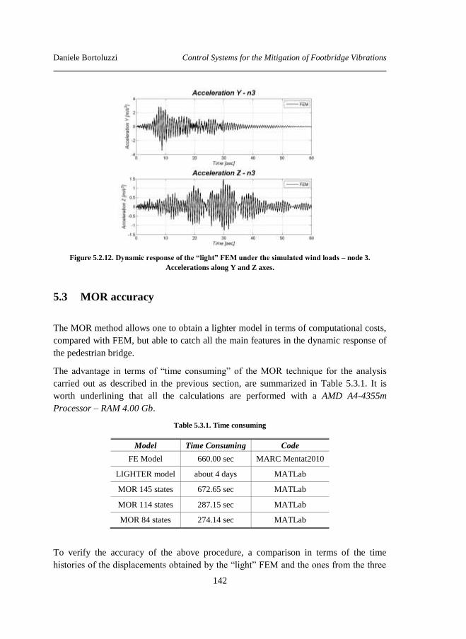
Daniele Bortoluzzi Control Systems for the Mitigation of Footbridge Vibrations
142
Figure 5.2.12. Dynamic response of the “light” FEM under the simulated wind loads – node 3.
Accelerations along Y and Z axes.
5.3 MOR accuracy
The MOR method allows one to obtain a lighter model in terms of computational costs,
compared with FEM, but able to catch all the main features in the dynamic response of
the pedestrian bridge.
The advantage in terms of “time consuming” of the MOR technique for the analysis
carried out as described in the previous section, are summarized in Table 5.3.1. It is
worth underlining that all the calculations are performed with a AMD A4-4355m
Processor – RAM 4.00 Gb.
Table 5.3.1. Time consuming
Model Time Consuming Code
FE Model 660.00 sec MARC Mentat2010
LIGHTER model about 4 days MATLab
MOR 145 states 672.65 sec MATLab
MOR 114 states 287.15 sec MATLab
MOR 84 states 274.14 sec MATLab
To verify the accuracy of the above procedure, a comparison in terms of the time
histories of the displacements obtained by the “light” FEM and the ones from the three
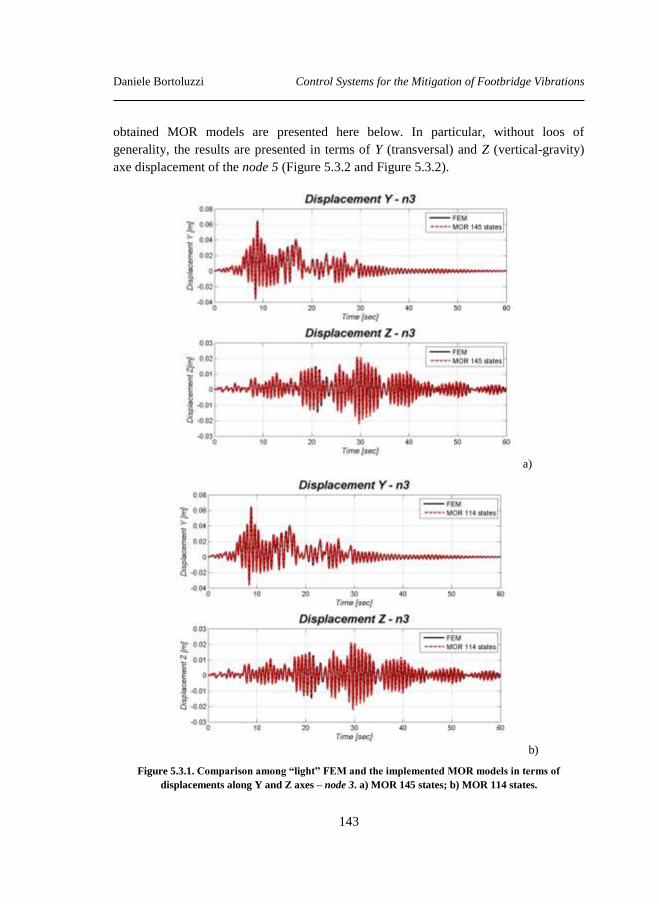
Daniele Bortoluzzi Control Systems for the Mitigation of Footbridge Vibrations
143
obtained MOR models are presented here below. In particular, without loos of
generality, the results are presented in terms of Y (transversal) and Z (vertical-gravity)
axe displacement of the node 5 (Figure 5.3.2 and Figure 5.3.2).
a)
b)
Figure 5.3.1. Comparison among “light” FEM and the implemented MOR models in terms of
displacements along Y and Z axes – node 3. a) MOR 145 states; b) MOR 114 states.
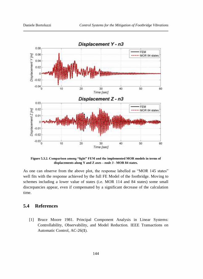
Daniele Bortoluzzi Control Systems for the Mitigation of Footbridge Vibrations
144
Figure 5.3.2. Comparison among “light” FEM and the implemented MOR models in terms of
displacements along Y and Z axes – node 3 - MOR 84 states.
As one can observe from the above plot, the response labelled as “MOR 145 states”
well fits with the response achieved by the full FE Model of the footbridge. Moving to
schemes including a lower value of states (i.e. MOR 114 and 84 states) some small
discrepancies appear, even if compensated by a significant decrease of the calculation
time.
5.4 References
[1] Bruce Moore 1981. Principal Component Analysis in Linear Systems:
Controllability, Observability, and Model Reduction. IEEE Transactions on
Automatic Control, AC-26(1).
Daniele Bortoluzzi Control Systems for the Mitigation of Footbridge Vibrations
145
[2] Glover, K. 1984. All optimal Hankel-norm approximations of linear
multivariable systems and their l∞-error bounds. Int. J. Control, 39, pp. 1115–
1193.
[3] Calberg K., Bou Mosleh C., Farhat C. 2011. Efficient non-linear model
reduction via a least squares Petrov-Galerkin projection and compressive
tensor approximations, International Journal for numerical methods in
engineering, 86, pp.155-181.
[4] Schilders W.H.A., van der Vorst H.A., Rommes J. 2008. Model Order
Reduction : Theory, Research Aspects and Applications, Springer.
[5] F. Casciati , S. Casciati, L. Faravelli, M. Franchinotti 2012. Model Order
Reduction vs. Structural Monitoring. On the Proceeding of 6th European
Workshop on Structural Health Monitoring – EWSHM2012 – Dresden,
Germany, July 3-6, 2012.
[6] Athanasios C. 2005. Approximation of large-scale dynamical systems, Society
for Industrial and Applied Mathematics, Philadelphia.
[7] A.C. Antoulas, 2002. Lectures on the approximation of large-scale dynamical
systems, Society for Industrial and Applied Mathematics, Philadelphia.
[8] Antoulas A.C., 2002. Frequency Domain Representation and Singular Value
Decomposition. Tech. Report, http://www.ece.rice.edu/~aca/
[9] Antoulas A.C., Sorensen D.C. , Zhou Y., 2002. On the decay rate of Hankel
singular values and related issues. Tech. Report, http://www.ece.rice.edu/~aca/
[10] Antoulas A.C., Sorensen D.C. e Gugercin S., 2001. A survey of the model
reduction methods for large-scale systems, Contemporary Mathematics, vol.
280, pp. 193-219.
[11] www.elitenetzwerk.beyern.de
[12] www.mscsoftware.com
[13] www.mathworks.it
[14] Casciati S., Faravelli L., 2014. Quantity vs. Quality in the Model Order
Reduction (MOR) of a Linear System , Smart Structures and Systems, 13 (1).
[15] Bortoluzzi, D., Casciati, F., Faravelli, L. 2014. Vibration mitigation in a
“cable-stayed-like” timber footbridge. On the Proceeding of the 6th World

Daniele Bortoluzzi Control Systems for the Mitigation of Footbridge Vibrations
146
Conference on Structural Control and Monitoring - 6WCSCM, Barcellona,
Spain, 15-17 July, 2014.
[16] NTC 2008. Norme tecniche per le costruzioni (in Italian) - D.M. 14 Gennaio
2008.
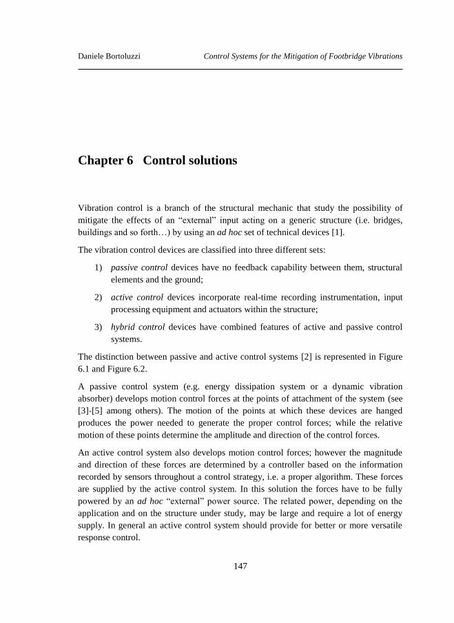
Daniele Bortoluzzi Control Systems for the Mitigation of Footbridge Vibrations
147
Chapter 6 Control solutions
Vibration control is a branch of the structural mechanic that study the possibility of
mitigate the effects of an “external” input acting on a generic structure (i.e. bridges,
buildings and so forth…) by using an ad hoc set of technical devices [1].
The vibration control devices are classified into three different sets:
1) passive control devices have no feedback capability between them, structural
elements and the ground;
2) active control devices incorporate real-time recording instrumentation, input
processing equipment and actuators within the structure;
3) hybrid control devices have combined features of active and passive control
systems.
The distinction between passive and active control systems [2] is represented in Figure
6.1 and Figure 6.2.
A passive control system (e.g. energy dissipation system or a dynamic vibration
absorber) develops motion control forces at the points of attachment of the system (see
[3]-[5] among others). The motion of the points at which these devices are hanged
produces the power needed to generate the proper control forces; while the relative
motion of these points determine the amplitude and direction of the control forces.
An active control system also develops motion control forces; however the magnitude
and direction of these forces are determined by a controller based on the information
recorded by sensors throughout a control strategy, i.e. a proper algorithm. These forces
are supplied by the active control system. In this solution the forces have to be fully
powered by an ad hoc “external” power source. The related power, depending on the
application and on the structure under study, may be large and require a lot of energy
supply. In general an active control system should provide for better or more versatile
response control.
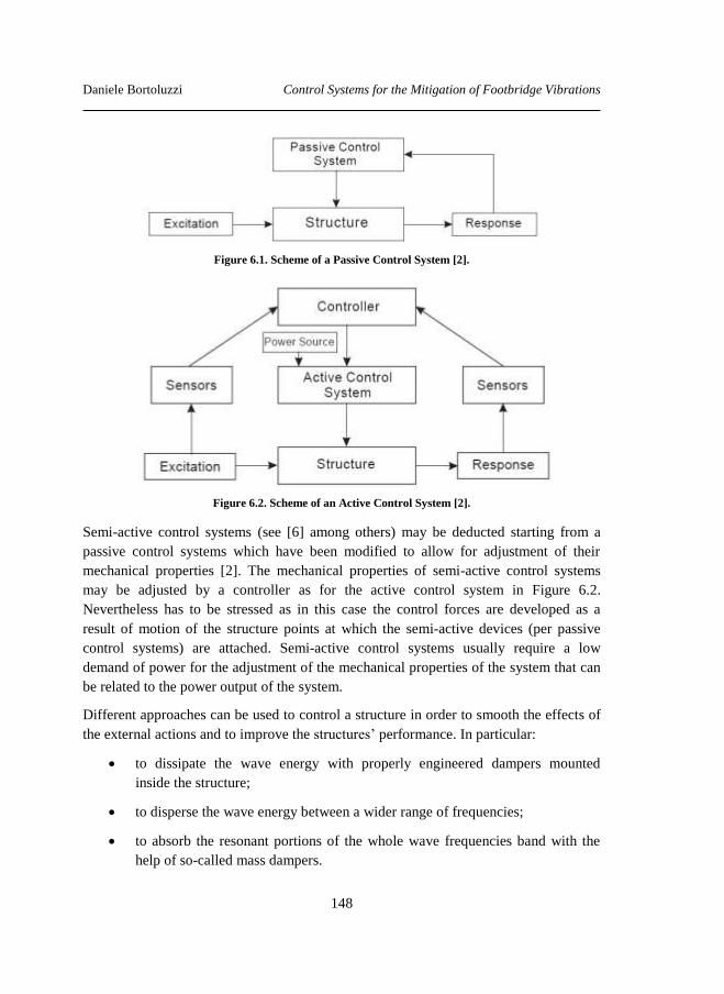
Daniele Bortoluzzi Control Systems for the Mitigation of Footbridge Vibrations
148
Figure 6.1. Scheme of a Passive Control System [2].
Figure 6.2. Scheme of an Active Control System [2].
Semi-active control systems (see [6] among others) may be deducted starting from a
passive control systems which have been modified to allow for adjustment of their
mechanical properties [2]. The mechanical properties of semi-active control systems
may be adjusted by a controller as for the active control system in Figure 6.2.
Nevertheless has to be stressed as in this case the control forces are developed as a
result of motion of the structure points at which the semi-active devices (per passive
control systems) are attached. Semi-active control systems usually require a low
demand of power for the adjustment of the mechanical properties of the system that can
be related to the power output of the system.
Different approaches can be used to control a structure in order to smooth the effects of
the external actions and to improve the structures’ performance. In particular:
to dissipate the wave energy with properly engineered dampers mounted
inside the structure;
to disperse the wave energy between a wider range of frequencies;
to absorb the resonant portions of the whole wave frequencies band with the
help of so-called mass dampers.
Daniele Bortoluzzi Control Systems for the Mitigation of Footbridge Vibrations
149
Within the last kind of the above devices one has: the so called TMD (tuned mass
dampers – see [4] among others) for the passive control approach, the AMD (active
mass dampers) for the active one, and the HMD (hybrid mass dampers) for the hybrid
control.
The following control solutions are introduced with reference of the “Trasaghis”
footbridge (see section 3.3) for the mitigation of the wind induced vibrations.
6.1 Passive control solutions
The finite element discretization leads one to write the standard dynamics equations in a
matrix form (see section 2.1):
,Mx Cx Kx ft t t t (6.1)
where, M, C and K are the mass, damping and stiffness matrices respectively, x are the
node generalized displacements, f are the nodal forces, t denotes the time and a “dot”
the time derivative as usual.
The governing relations with tuned mass dampers add forces at given locations [2] as
follows:
,Mx Cx Kx f T cz kzt t t t t t (6.2)
where T is a topological matrix while the matrices c and k contain, for each TMD, the
damping coefficient c and the stiffness k. The variable z is the relative displacement of
the added mass of the single TMD at the anchorage point, so that:
mz t cz t kz t mx t , (6.3)
where m is the added mass and is the displacement of the hanging point in the direction
of the TMD degree of freedom z.
The standard design of a single TMD device requires the tuning of the frequency and
the added mass, or better the ratio between this secondary mass and the primary one,
for a 1-DOF system. The damping and stiffness coefficients, c and k in equation (6.3),
depend on the ratio as reported in [2], [7] and [8]-[11] among others. A first extension
to MDOF’s primary systems, see [2], was developed for the design of TMD devices in
frames with lumped masses at each stories.
Let’s consider the case of a N-DOF damped structure. If a single TMD is installed in
correspondence to the j-th DOF, the equations of motion can be written as:
Daniele Bortoluzzi Control Systems for the Mitigation of Footbridge Vibrations
150
Mx Cx Kx f j j jt t t t d c z t k z t , (6.4)
where jis the standard diagonal matrix of Kronecker indexes. To complete the
formulation the above j-th equation have to be coupled with equation (6.3) where all the
coefficients come with the index j; that is:
Mx Cx Kx f j j j
j j
t t t t d c z t k z t
mz t c z t k z t mx t
. (6.5)
If the TMD is to be designed for the i-th structural mode with modal properties Mi , Ki
and Ci , the design problem is similar to the design of a TMD device for a 1-DOF
structure. Indeed, introducing the modal coordinate y(t), the resulting modal equation
can be written as follows:
[ ( ) ( )]f T
i i i i j j jM y t C y t K y t t d c z t k z t . (6.6)
Two critical problems, not usually considered in the standard design procedure of a
TMD(s) device(s), are here discussed:
1) when using a commercial software for the finite element analyses (FEA), the
modal mass normalization is pursued toward having that matrix built as an
identity matrix;
2) when the primary system is a bridge, there are longitudinal and transversal
symmetries which suggest to hang several identical devices at different points.
This is especially true when the vibration to be mitigated give rise to local
vibration problems, instead than the case when the vibration problems
originates from an oscillation of the whole structural system.
The first aspect requires17 to obtain from the numerical model the mass, damping and
stiffness matrices, and to work directly on them toward the suitable normalization
procedure for instance working in the MatLAB environment [12].
Due to the structural, material and geometry symmetry of the “Trasaghis” footbridge, it
is reasonable to assume that the vibration of the structural elements occurs in phase or in
opposition of phase, as well as in combined modes. Thus, the TMD system becomes a
multiple tuned mass damper, with devices hung in several companion points.
Two situations may be identified:
17 If no specific options are provided in the FEA software options.
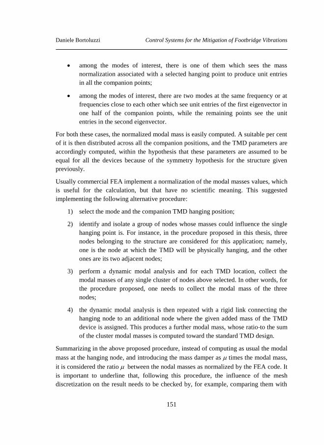
Daniele Bortoluzzi Control Systems for the Mitigation of Footbridge Vibrations
151
among the modes of interest, there is one of them which sees the mass
normalization associated with a selected hanging point to produce unit entries
in all the companion points;
among the modes of interest, there are two modes at the same frequency or at
frequencies close to each other which see unit entries of the first eigenvector in
one half of the companion points, while the remaining points see the unit
entries in the second eigenvector.
For both these cases, the normalized modal mass is easily computed. A suitable per cent
of it is then distributed across all the companion positions, and the TMD parameters are
accordingly computed, within the hypothesis that these parameters are assumed to be
equal for all the devices because of the symmetry hypothesis for the structure given
previously.
Usually commercial FEA implement a normalization of the modal masses values, which
is useful for the calculation, but that have no scientific meaning. This suggested
implementing the following alternative procedure:
1) select the mode and the companion TMD hanging position;
2) identify and isolate a group of nodes whose masses could influence the single
hanging point is. For instance, in the procedure proposed in this thesis, three
nodes belonging to the structure are considered for this application; namely,
one is the node at which the TMD will be physically hanging, and the other
ones are its two adjacent nodes;
3) perform a dynamic modal analysis and for each TMD location, collect the
modal masses of any single cluster of nodes above selected. In other words, for
the procedure proposed, one needs to collect the modal mass of the three
nodes;
4) the dynamic modal analysis is then repeated with a rigid link connecting the
hanging node to an additional node where the given added mass of the TMD
device is assigned. This produces a further modal mass, whose ratio to the sum
of the cluster modal masses is computed toward the standard TMD design.
Summarizing in the above proposed procedure, instead of computing as usual the modal
mass at the hanging node, and introducing the mass damper as times the modal mass,
it is considered the ratio between the nodal masses as normalized by the FEA code. It
is important to underline that, following this procedure, the influence of the mesh
discretization on the result needs to be checked by, for example, comparing them with
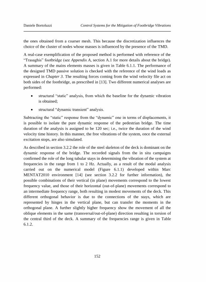
Daniele Bortoluzzi Control Systems for the Mitigation of Footbridge Vibrations
152
the ones obtained from a coarser mesh. This because the discretization influences the
choice of the cluster of nodes whose masses is influenced by the presence of the TMD.
A real-case exemplification of the proposed method is performed with reference of the
“Trasaghis” footbridge (see Appendix A, section A.1 for more details about the bridge).
A summary of the mains elements masses is given in Table 6.1.1. The performance of
the designed TMD passive solution is checked with the reference of the wind loads as
expressed in Chapter 3. The resulting forces coming from the wind velocity file act on
both sides of the footbridge, as prescribed in [13]. Two different numerical analyses are
performed:
structural “static” analysis, from which the baseline for the dynamic vibration
is obtained;
structural “dynamic transient” analysis.
Subtracting the “static” response from the “dynamic” one in terms of displacements, it
is possible to isolate the pure dynamic response of the pedestrian bridge. The time
duration of the analysis is assigned to be 120 sec; i.e., twice the duration of the wind
velocity time history. In this manner, the free vibrations of the system, once the external
excitation stops, are also simulated.
As described in section 3.2.2 the role of the steel skeleton of the deck is dominant on the
dynamic response of the bridge. The recorded signals from the in situ campaigns
confirmed the role of the long tubular stays in determining the vibration of the system at
frequencies in the range from 1 to 2 Hz. Actually, as a result of the modal analysis
carried out on the numerical model (Figure 6.1.1) developed within Marc
MENTAT2010 environment [14] (see section 3.2.2 for further information), the
possible combinations of their vertical (in plane) movements correspond to the lowest
frequency value, and those of their horizontal (out-of-plane) movements correspond to
an intermediate frequency range, both resulting in modest movements of the deck. This
different orthogonal behavior is due to the connections of the stays, which are
represented by hinges in the vertical plane, but can transfer the moments in the
orthogonal plane. A further slightly higher frequency show the movement of all the
oblique elements in the same (transversal/out-of-plane) direction resulting in torsion of
the central third of the deck. A summary of the frequencies range is given in Table
6.1.2.
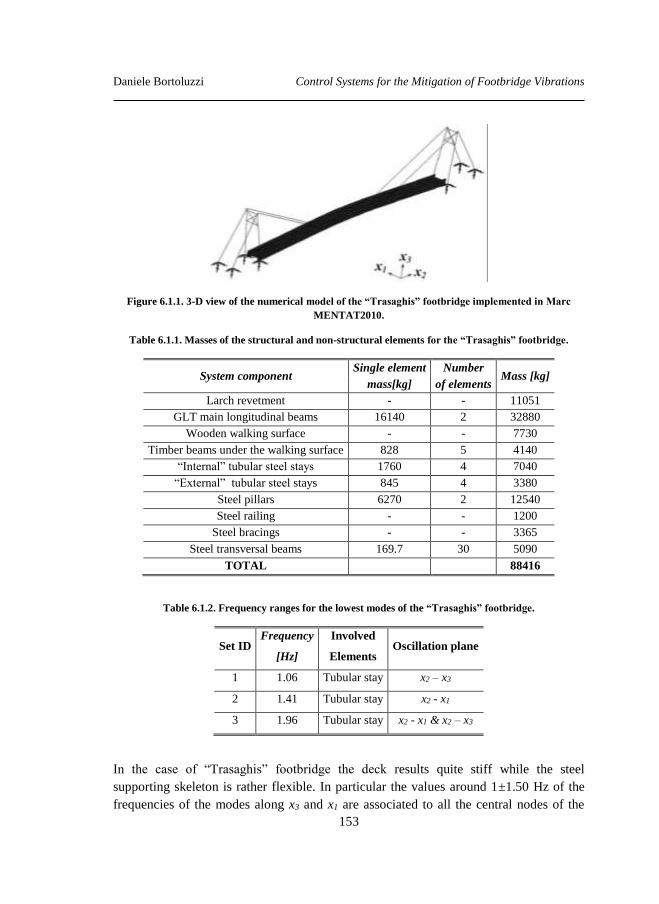
Daniele Bortoluzzi Control Systems for the Mitigation of Footbridge Vibrations
153
Figure 6.1.1. 3-D view of the numerical model of the “Trasaghis” footbridge implemented in Marc
MENTAT2010.
Table 6.1.1. Masses of the structural and non-structural elements for the “Trasaghis” footbridge.
System component Single element Number
Mass [kg] mass[kg] of elements
Larch revetment - - 11051
GLT main longitudinal beams 16140 2 32880
Wooden walking surface - - 7730
Timber beams under the walking surface 828 5 4140
“Internal” tubular steel stays 1760 4 7040
“External” tubular steel stays 845 4 3380
Steel pillars 6270 2 12540
Steel railing - - 1200
Steel bracings - - 3365
Steel transversal beams 169.7 30 5090
TOTAL 88416
Table 6.1.2. Frequency ranges for the lowest modes of the “Trasaghis” footbridge.
Set ID Frequency
[Hz]
Involved
Elements Oscillation plane
1 1.06 Tubular stay x2 – x3
2 1.41 Tubular stay x2 - x1
3 1.96 Tubular stay x2 - x1 & x2 – x3
In the case of “Trasaghis” footbridge the deck results quite stiff while the steel
supporting skeleton is rather flexible. In particular the values around 1±1.50 Hz of the
frequencies of the modes along x3 and x1 are associated to all the central nodes of the
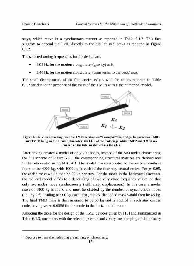
Daniele Bortoluzzi Control Systems for the Mitigation of Footbridge Vibrations
154
stays, which move in a synchronous manner as reported in Table 6.1.2. This fact
suggests to append the TMD directly to the tubular steel stays as reported in Figure
6.1.2.
The selected tuning frequencies for the design are:
1.05 Hz for the motion along the x3 (gravity) axis;
1.40 Hz for the motion along the x1 (transversal to the deck) axis.
The small discrepancies of the frequencies values with the values reported in Table
6.1.2 are due to the presence of the mass of the TMDs within the numerical model.
Figure 6.1.2. View of the implemented TMDs solution on “Trasaghis” footbridge. In particular TMD1
and TMD3 hung on the tubular elements in the l.h.s. of the footbridge, while TMD2 and TMD4 are
hanged on the tubular elements in the r.h.s.
After having created a model of only 200 nodes, instead of the 500 nodes charactering
the full scheme of Figure 6.1.1, the corresponding structural matrices are derived and
further elaborated using MatLAB. The modal mass associated to the vertical mode is
found to be 4000 kg, with 1000 kg in each of the four stay central nodes. For =0.05,
the added mass would then be 50 kg per stay. For the mode in the horizontal direction,
the reduced model yields to a decoupling of two very close frequency values, so that
only two nodes move synchronously (with unity displacement). In this case, a modal
mass of 1800 kg is found and must be divided by the number of synchronous nodes
(i.e., by 218), leading to 900 kg each. For =0.05, the added mass would then be 45 kg.
The final TMD mass is then assumed to be 50 kg and is applied at each stay central
node, having set =0.0556 for the mode in the horizontal direction.
Adopting the table for the design of the TMD devices given by [15] and summarized in
Table 6.1.3, one enters with the selected value and a very low damping of the primary
18 Because two are the nodes that are moving synchronously.
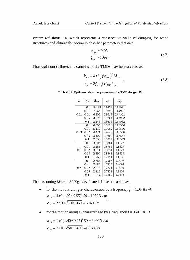
Daniele Bortoluzzi Control Systems for the Mitigation of Footbridge Vibrations
155
system (of about 1%, which represents a conservative value of damping for wood
structures) and obtains the optimum absorber parameters that are:
0.95
10%
opt
opt
. (6.7)
Thus optimum stiffness and damping of the TMDs may be evaluated as:
2
24
2
opt opt TMD
opt opt TMD opt
k f M
c M k
. (6.8)
Table 6.1.3. Optimum absorber parameters for TMD design [15].
s Ropt s opt
0.01
0
0.01 0.02
0.05
0.1
10.138
7.743 6.205
3.798
2.249
0.9876
0.9859 0.9819
0.9704
0.9436
0.04981
0.04981 0.04981
0.04982
0.04982
0.03
0 0.01
0.02
0.05
0.1
6.058 5.110
4.424
3.109
2.036
0.9636 0.9592
0.9545
0.9380
0.9032
0.08566 0.08566
0.08566
0.08567
0.08569
0.1
0
0.01 0.02
0.05
0.1
3.602
3.285 3.014
2.399
1.765
0.8861
0.8789 0.8714
0.8468
0.7991
0.1527
0.1527 0.1528
0.1529
0.1531
0.2
0 0.01
0.02
0.05 0.1
2.865 2.680
2.516
2.113 1.649
0.7906 0.7815
0.7721
0.7421 0.6862
0.2097 0.2098
0.2099
0.2103 0.2112
Then assuming MTMD = 50 Kg as evaluated above one achieves:
for the motions along x3 characterized by a frequency f = 1.05 Hz
224 1.05 0.95 50 1950 /
2 0.1 50 1950 60 /
opt
opt
k N m
c Ns m
;
for the motion along x1 characterized by a frequency f = 1.40 Hz
224 1.40 0.95 50 3400 /
2 0.1 50 3400 80 /
opt
opt
k N m
c Ns m
.

Daniele Bortoluzzi Control Systems for the Mitigation of Footbridge Vibrations
156
Summarizing, for this proposed TMD system, called TMD_A, the main features are
collected in Table 6.1.4
Table 6.1.4. Main features of the TMD_A solution.
ID Value
mass MTMD 50 Kg each TMD
stiffness kx1 3400 N/m
damping cx1 80 Ns/m
stiffness kx3 1950 N/m
damping cx3 60 Ns/m
The alternative design approach consists of the following steps:
1) identify the sub-system whose vibrations have to be mitigated. In the
considered case study, it is represented by the four tubular stays of total mass
1760 Kg (Table 6.1.1). Each stay is discretized into four hollow elements
leading to a nodal mass of 440 kg per node. For further calculations, the
attention is focused on the three internal nodes.
2) when considering the mode at 1.05 Hz and a rigid link to the added mass, the
modal analysis provides the following (dimensionless) modal masses as
provided by the FEA coded employed [14]: 3.22, 6.55 and 4.52 for the three
internal nodes, and 0.77 for the added mass. These values correspond to
5.39%; the error is 7% with respect to the “lightest” FE mesh, and it will be
seen to be dependent on the discretization.
3) for the mode at 1.40 Hz and a rigid link to the added mass, the modal analysis
provides the following (dimensionless) modal masses: 4.09, 7.31 and 4.12 for
the three internal nodes, and 0.87 for the added mass. The resulting value of
is 5.61%, with an even lower error with respect to the “lightest” FE mesh.
Thus, it is seen that the alternative approach leads to consistent results within a suitable
degree of approximation. If the reasoning is repeated with a model in which the stays
are just discretized into two elements, one obtains higher over-estimations of the values
of ; namely, 0.75 and 0.76 in the two directions x3 and x1, respectively.
The design of the implemented TMD’s solution is summarized in Figure 6.1.3. Each
TMD are realized by a steel hollow cylinder of radius R = 35 cm, thickness t = 4 mm
and length l = 64 cm. The design choices allow to fit well with both aesthetics and
structural aspects; in fact it is hanged in the hinge located in the middle of the stay.
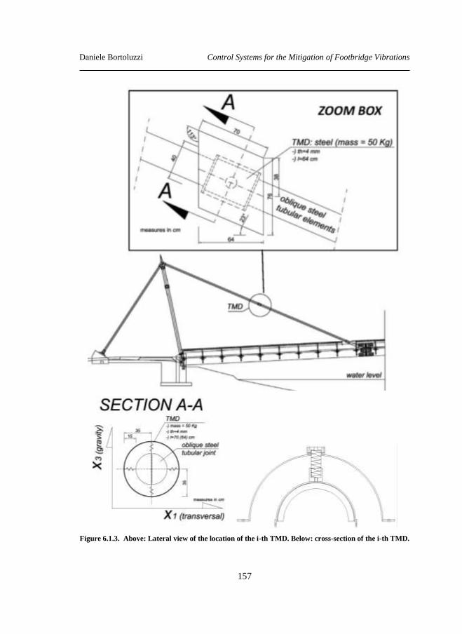
Daniele Bortoluzzi Control Systems for the Mitigation of Footbridge Vibrations
157
Figure 6.1.3. Above: Lateral view of the location of the i-th TMD. Below: cross-section of the i-th TMD.
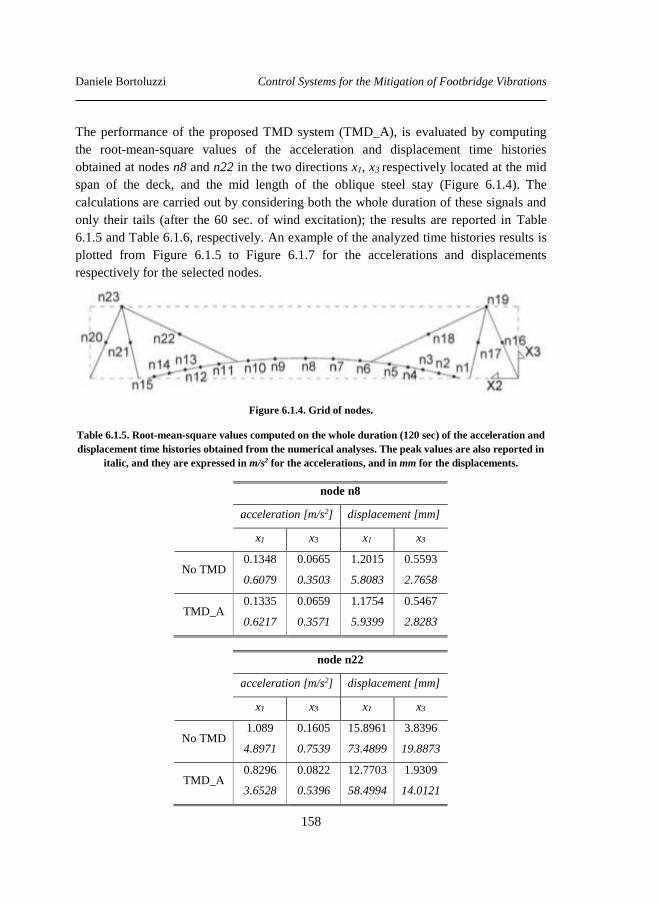
Daniele Bortoluzzi Control Systems for the Mitigation of Footbridge Vibrations
158
The performance of the proposed TMD system (TMD_A), is evaluated by computing
the root-mean-square values of the acceleration and displacement time histories
obtained at nodes n8 and n22 in the two directions x1, x3 respectively located at the mid
span of the deck, and the mid length of the oblique steel stay (Figure 6.1.4). The
calculations are carried out by considering both the whole duration of these signals and
only their tails (after the 60 sec. of wind excitation); the results are reported in Table
6.1.5 and Table 6.1.6, respectively. An example of the analyzed time histories results is
plotted from Figure 6.1.5 to Figure 6.1.7 for the accelerations and displacements
respectively for the selected nodes.
Figure 6.1.4. Grid of nodes.
Table 6.1.5. Root-mean-square values computed on the whole duration (120 sec) of the acceleration and
displacement time histories obtained from the numerical analyses. The peak values are also reported in
italic, and they are expressed in m/s2 for the accelerations, and in mm for the displacements.
node n8
acceleration [m/s2] displacement [mm]
x1 x3 x1 x3
No TMD 0.1348
0.6079
0.0665
0.3503
1.2015
5.8083
0.5593
2.7658
TMD_A 0.1335
0.6217
0.0659
0.3571
1.1754
5.9399
0.5467
2.8283
node n22
acceleration [m/s2] displacement [mm]
x1 x3 x1 x3
No TMD 1.089
4.8971
0.1605
0.7539
15.8961
73.4899
3.8396
19.8873
TMD_A 0.8296
3.6528
0.0822
0.5396
12.7703
58.4994
1.9309
14.0121
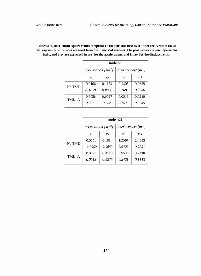
Daniele Bortoluzzi Control Systems for the Mitigation of Footbridge Vibrations
159
Table 6.1.6. Root- mean-square values computed on the tails (the first 15 sec after the event) of the of
the response time histories obtained from the numerical analyses. The peak values are also reported in
italic, and they are expressed in m/s2 for the accelerations, and in mm for the displacements.
node n8
acceleration [m/s2] displacement [mm]
x1 x3 x1 x3
No TMD 0.0108
-0.0121
0.1174
0.0896
0.1405
0.1686
0.0669
0.0580
TMD_A 0.0058
0.0011
0.0597
-0.2571
0.0513
0.1547
0.0239
0.0735
node n22
acceleration [m/s2] displacement [mm]
x1 x3 x1 x3
No TMD 0.0051
-0.0059
0.1014
0.0883
1.5997
0.6423
2.4365
0.2851
TMD_A 0.0027
0.0012
0.0113
0.0275
0.9543
0.2421
0.2498
0.1143
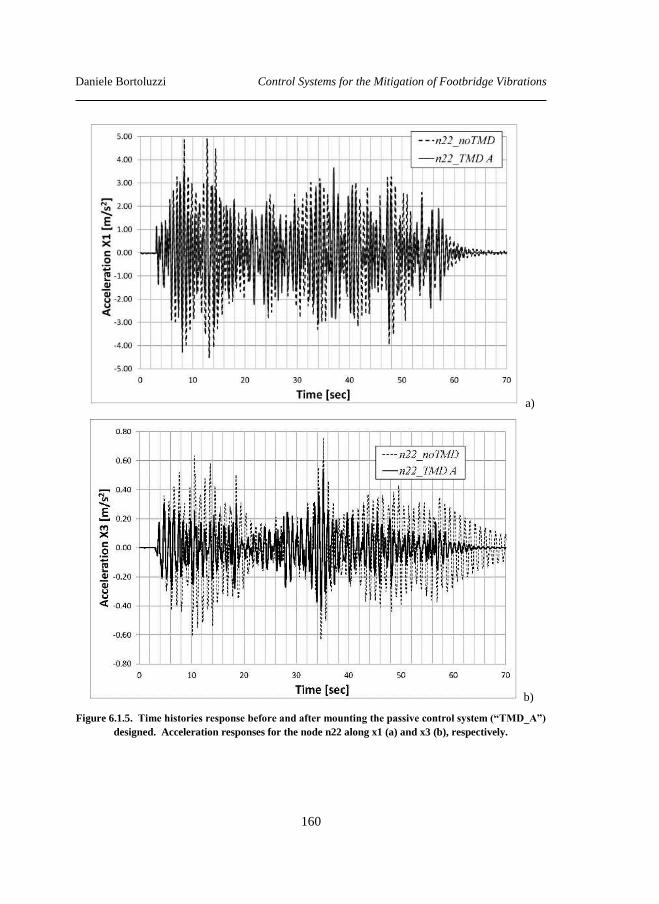
Daniele Bortoluzzi Control Systems for the Mitigation of Footbridge Vibrations
160
a)
b)
Figure 6.1.5. Time histories response before and after mounting the passive control system (“TMD_A”)
designed. Acceleration responses for the node n22 along x1 (a) and x3 (b), respectively.
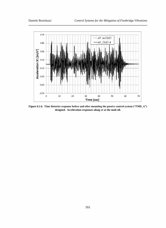
Daniele Bortoluzzi Control Systems for the Mitigation of Footbridge Vibrations
161
Figure 6.1.6. Time histories response before and after mounting the passive control system (“TMD_A”)
designed. Acceleration responses along x1 at the node n8.
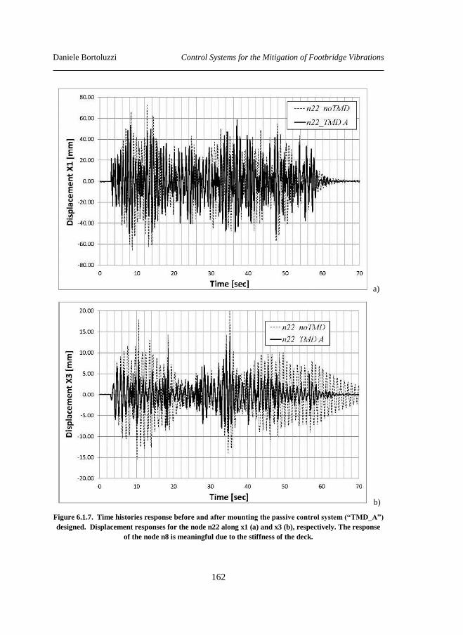
Daniele Bortoluzzi Control Systems for the Mitigation of Footbridge Vibrations
162
a)
b)
Figure 6.1.7. Time histories response before and after mounting the passive control system (“TMD_A”)
designed. Displacement responses for the node n22 along x1 (a) and x3 (b), respectively. The response
of the node n8 is meaningful due to the stiffness of the deck.
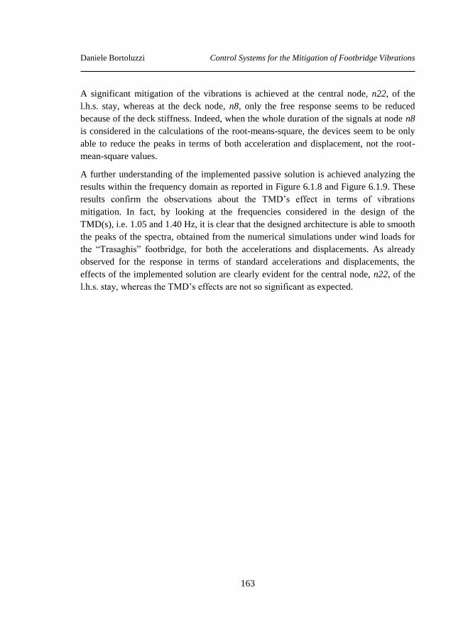
Daniele Bortoluzzi Control Systems for the Mitigation of Footbridge Vibrations
163
A significant mitigation of the vibrations is achieved at the central node, n22, of the
l.h.s. stay, whereas at the deck node, n8, only the free response seems to be reduced
because of the deck stiffness. Indeed, when the whole duration of the signals at node n8
is considered in the calculations of the root-means-square, the devices seem to be only
able to reduce the peaks in terms of both acceleration and displacement, not the root-
mean-square values.
A further understanding of the implemented passive solution is achieved analyzing the
results within the frequency domain as reported in Figure 6.1.8 and Figure 6.1.9. These
results confirm the observations about the TMD’s effect in terms of vibrations
mitigation. In fact, by looking at the frequencies considered in the design of the
TMD(s), i.e. 1.05 and 1.40 Hz, it is clear that the designed architecture is able to smooth
the peaks of the spectra, obtained from the numerical simulations under wind loads for
the “Trasaghis” footbridge, for both the accelerations and displacements. As already
observed for the response in terms of standard accelerations and displacements, the
effects of the implemented solution are clearly evident for the central node, n22, of the
l.h.s. stay, whereas the TMD’s effects are not so significant as expected.

Daniele Bortoluzzi Control Systems for the Mitigation of Footbridge Vibrations
164
a)
b)
c)
Figure 6.1.8. Response spectra as obtained from the acceleration responses along x1 (a) and x3 (b) at
the node n22; and (c) from the acceleration response along x1 at the node n8, before and after the
installation of the passive control system (TMD_A).
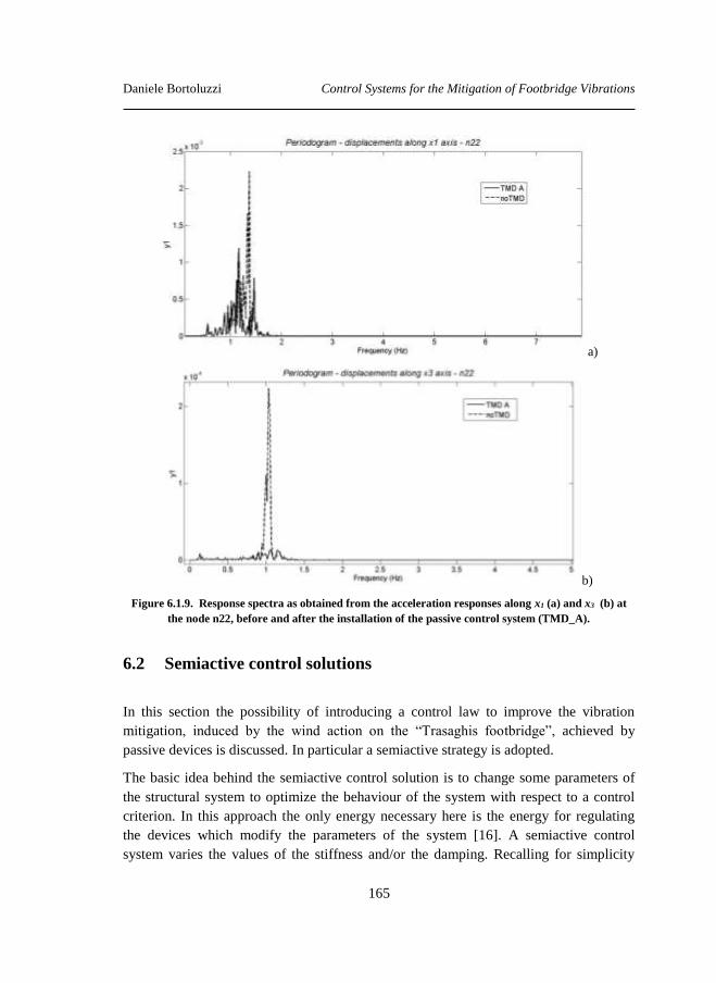
Daniele Bortoluzzi Control Systems for the Mitigation of Footbridge Vibrations
165
a)
b)
Figure 6.1.9. Response spectra as obtained from the acceleration responses along x1 (a) and x3 (b) at
the node n22, before and after the installation of the passive control system (TMD_A).
6.2 Semiactive control solutions
In this section the possibility of introducing a control law to improve the vibration
mitigation, induced by the wind action on the “Trasaghis footbridge”, achieved by
passive devices is discussed. In particular a semiactive strategy is adopted.
The basic idea behind the semiactive control solution is to change some parameters of
the structural system to optimize the behaviour of the system with respect to a control
criterion. In this approach the only energy necessary here is the energy for regulating
the devices which modify the parameters of the system [16]. A semiactive control
system varies the values of the stiffness and/or the damping. Recalling for simplicity

Daniele Bortoluzzi Control Systems for the Mitigation of Footbridge Vibrations
166
and without loss of generality the equation of motion for a 1-DOF system (see equation
(2.3)), this can be represented simply as:
2
0 02 C
F tx t x t x t f
m , (6.9)
where the control force in defined as:
2
0 02C C Kf t x t t x t , (6.10)
in which C t and K t are functions of time. Control systems where parameters of
the system can be varied are called variable structure systems.
This implementation is mainly motivated by the fact that the good performance of the
passive solutions, as observed in section 6.1 is restricted to a narrow window around the
tuning frequency chosen during the device design [7].
Nevertheless, the global cost of the footbridge suggests to restrict the investigation
within very simple technological solutions. Thus, first of all a limitation is set on the
available feedback; the relative displacement z and velocity z between the anchorage
point and the secondary mass seems to be a suitable solution. A second limitation
concerns the simplicity of the control law, which is generally made of a premise (IF)
and a consequence (THEN). In this way a good compromise between the cost and
efficacy of the solution can be achieved.
One assumes that, at each time step, the premise relies on the instantaneous values of
the relative displacement and velocity introduced above, while the consequence is on
the value of the device output force. In particular the simple “bang-bang control” is
adopted [16].
Bang-bang control provides a simple and yet often effective approach. It is usually
applied for dissipative devices in order to increase their capabilities in dissipating
energy with respect to a classical passive device. The working principle of this control,
approach can so summarized:
when the relative displacement and the relative velocity of the two ends of the
damping device are in the same direction, bang-bang control acts in the
direction of increasing the forces in the device to a maximum value;
vice-versa when the relative displacement and the relative velocity of the ends
of the device are in opposite directions, the control law decreases the value of
the forces to a minimum in order to make the device movement as easy as
possible.
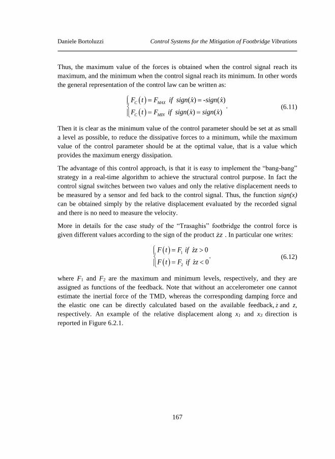
Daniele Bortoluzzi Control Systems for the Mitigation of Footbridge Vibrations
167
Thus, the maximum value of the forces is obtained when the control signal reach its
maximum, and the minimum when the control signal reach its minimum. In other words
the general representation of the control law can be written as:
( ) - ( ).
( ) ( )
C MAX
C MIN
F t F if sign x sign x
F t F if sign x sign x
(6.11)
Then it is clear as the minimum value of the control parameter should be set at as small
a level as possible, to reduce the dissipative forces to a minimum, while the maximum
value of the control parameter should be at the optimal value, that is a value which
provides the maximum energy dissipation.
The advantage of this control approach, is that it is easy to implement the “bang-bang”
strategy in a real-time algorithm to achieve the structural control purpose. In fact the
control signal switches between two values and only the relative displacement needs to
be measured by a sensor and fed back to the control signal. Thus, the function sign(x)
can be obtained simply by the relative displacement evaluated by the recorded signal
and there is no need to measure the velocity.
More in details for the case study of the “Trasaghis” footbridge the control force is
given different values according to the sign of the product zz . In particular one writes:
1
2
0.
0
F t F if zz
F t F if zz
(6.12)
where F1 and F2 are the maximum and minimum levels, respectively, and they are
assigned as functions of the feedback. Note that without an accelerometer one cannot
estimate the inertial force of the TMD, whereas the corresponding damping force and
the elastic one can be directly calculated based on the available feedback, z and z,
respectively. An example of the relative displacement along x1 and x3 direction is
reported in Figure 6.2.1.
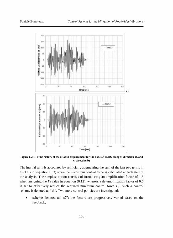
Daniele Bortoluzzi Control Systems for the Mitigation of Footbridge Vibrations
168
a)
b)
Figure 6.2.1. Time history of the relative displacement for the node of TMD2 along x1 direction a), and
x3 direction b).
The inertial term is accounted by artificially augmenting the sum of the last two terms in
the l.h.s. of equation (6.3) when the maximum control force is calculated at each step of
the analysis. The simplest option consists of introducing an amplification factor of 1.8
when assigning the F2 value in equation (6.12), whereas a de-amplification factor of 0.6
is set to effectively reduce the required minimum control force F1. Such a control
scheme is denoted as “s1”. Two more control policies are investigated:
scheme denoted as “s2”: the factors are progressively varied based on the
feedback;
Daniele Bortoluzzi Control Systems for the Mitigation of Footbridge Vibrations
169
scheme denoted as “s3”: a contribution which replaces the inertia term by an
estimate is added.
To check the performance of the semiactive solution, three different configurations for
the TMDs are considered:
1) the first one is the TMD_A solution as evaluated in section 6.1 (see Table 6.1.4
for the main features of this solution);
2) the second one, called TMD_B solution, is obtained tuning the TMD at the
frequency f = 1.96 Hz (that regards both the motion along x1 and x3 as from
Table 6.1.2). Following the standard design of the TMD described in section
6.1 and given by [15], assuming a mass of the singular TMD equal to MTMD =
50 Kg the stiffness of the TMD may be evaluated as: f = 1.96 Hz
224 1.96 0.95 50 6727 /optk N m for both x1 and x3 directions. The
damping is assumed conservatively equal to case TMD_A along x1, that is
480 /optc Ns m , for both the direction x1 and x3;
3) the third architecture, called TMD_C solution, is obtained mixing the two
previous solutions. It mounts the devices of TMD_A in the positions denoted
as TMD1 and TMD4 in Figure 6.1.2 and the devices of TMD B in the other
two locations (Figure 6.2.2).
Figure 6.2.2. View of the TMD_C of the “Trasaghis” footbridge.
The main results achieved by the semiactive architecture above described are
summarized here below. In particular the results are represented in terms of the root-
mean-square for the whole signal (Table 6.2.1) of accelerations and displacements, and
in terms of the root-mean-square of the first 15 sec after the event (Table 6.2.2) for both
the signal of accelerations and displacements. The control solutions are denoted by the
same acronym as the corresponding strategies adopted; i.e. “si, i=1,2,3”.
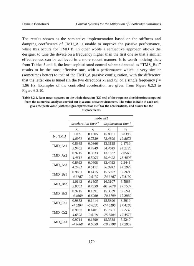
Daniele Bortoluzzi Control Systems for the Mitigation of Footbridge Vibrations
170
The results shown as the semiactive implementation based on the stiffness and
damping coefficients of TMD_A is unable to improve the passive performance,
while this occurs for TMD B. In other words a semiactive approach allows the
designer to tune the device on a frequency higher than the first one so that a similar
effectiveness can be achieved in a more robust manner. It is worth noticing that,
from Tables 5 and 6, the least sophisticated control scheme denoted as “TMS_Bs1”
results to be the most effective one, with a performance which is very similar
(sometimes better) to that of the TMD_A passive configuration, with the difference
that the latter one is tuned (in the two directions x1 and x3) on a single frequency f =
1.96 Hz. Examples of the controlled acceleration are given from Figure 6.2.3 to
Figure 6.2.10.
Table 6.2.1. Root-mean-squares on the whole duration (120 sec) of the response time histories computed
from the numerical analyses carried out in a semi-active environment. The value in italic in each cell
gives the peak value (with its sign) expressed as m/s2 for the accelerations, and as mm for the
displacements.
node n22
acceleration [m/s2] displacement [mm]
x1 x3 x1 x3
No TMD 1.089
4.8971
0.1605
0.7539
15.8961
73.4899
3.8396
19.8873
TMD_As1 0.8365
3.9462
0.0866
0.4949
12.3125
54.4649
2.1739
14.2123
TMD_As2 0.9215
4.4611
0.0833
0.5003
13.1832
59.4422
2.0563
13.4807
TMD_As3 0.8923
4.2431
0.0908
0.5171
12.4023
56.3241
2.2441
14.2929
TMD_Bs1 0.9861
-4.6187
0.1415
-0.6132
15.5892
-74.6187
3.5921
17.4190
TMD_Bs2 1.0143
5.0301
0.1605
0.7539
16.3107
-81.9679
3.5868
17.7537
TMD_Bs3 0.9715
-4.4669
0.1391
0.6060
15.3339
-70.3799
3.5241
17.2960
TMD_Cs1 0.9858
-4.6184
0.1414
-0.6130
15.5890
-74.6185
3.5919
17.4188
TMD_Cs2 0.9937
4.6502
0.1401
-0.6104
15.7661
-75.6504
3.5537
17.4577
TMD_Cs3 0.9714
-4.4668
0.1390
0.6059
15.3338
-70.3798
3.5240
17.2959
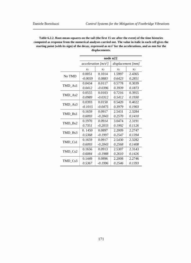
Daniele Bortoluzzi Control Systems for the Mitigation of Footbridge Vibrations
171
Table 6.2.2. Root-mean-squares on the tail (the first 15 sec after the event) of the time histories
computed as response from the numerical analyses carried out. The value in italic in each cell gives the
starting point (with its sign) of the decay, expressed as m/s2 for the accelerations, and as mm for the
displacements.
node n22
acceleration [m/s2] displacement [mm]
x1 x3 x1 x3
No TMD 0.0051
-0.0059
0.1014
0.0883
1.5997
0.6423
2.4365
0.2851
TMD_As1 0.0434
0.0412
0.0117
-0.0396
0.5778
0.3939
0.3039
0.1873
TMD_As2 0.0555
0.0989
0.0103
-0.0312
0.7216
0.5412
0.3955
0.1930
TMD_As3 0.0393
-0.1015
0.0150
-0.0475
0.5420
0.3979
0.4022
0.1903
TMD_Bs1 0.1659
0.6093
0.0917
-0.2043
2.5431
0.2570
2.3284
0.1410
TMD_Bs2 0.1970
0.7351
0.0914
-0.2033
3.0474
0.1992
2.3191
0.1126
TMD_Bs3 0. 1450
0.5368
0.0897
-0.1997
2.2009
0.2547
2.2747
0.1394
TMD_Cs1 0.1659
0.6093
0.0917
-0.2043
2.5430
0.2568
2.3282
0.1408
TMD_Cs2 0.1656
0.6084
0.0913
-0.1988
2.5307
0.2610
2.3143
0.1426
TMD_Cs3 0.1449
0.5367
0.0896
-0.1996
2.2008
0.2546
2.2746
0.1393
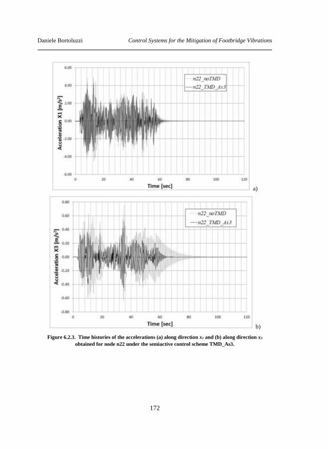
Daniele Bortoluzzi Control Systems for the Mitigation of Footbridge Vibrations
172
a)
b)
Figure 6.2.3. Time histories of the accelerations (a) along direction x1 and (b) along direction x3
obtained for node n22 under the semiactive control scheme TMD_As3.
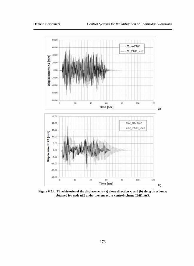
Daniele Bortoluzzi Control Systems for the Mitigation of Footbridge Vibrations
173
a)
b)
Figure 6.2.4. Time histories of the displacements (a) along direction x1 and (b) along direction x3
obtained for node n22 under the semiactive control scheme TMD_As3.
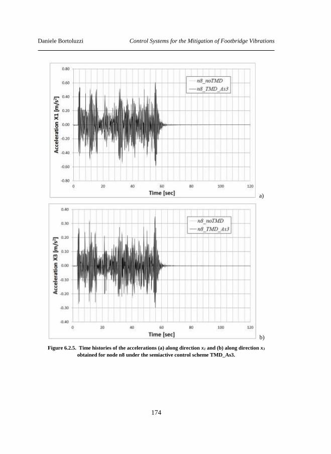
Daniele Bortoluzzi Control Systems for the Mitigation of Footbridge Vibrations
174
a)
b)
Figure 6.2.5. Time histories of the accelerations (a) along direction x1 and (b) along direction x3
obtained for node n8 under the semiactive control scheme TMD_As3.
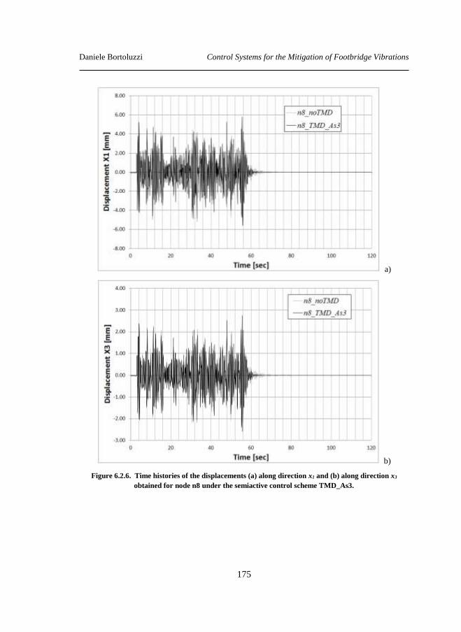
Daniele Bortoluzzi Control Systems for the Mitigation of Footbridge Vibrations
175
a)
b)
Figure 6.2.6. Time histories of the displacements (a) along direction x1 and (b) along direction x3
obtained for node n8 under the semiactive control scheme TMD_As3.
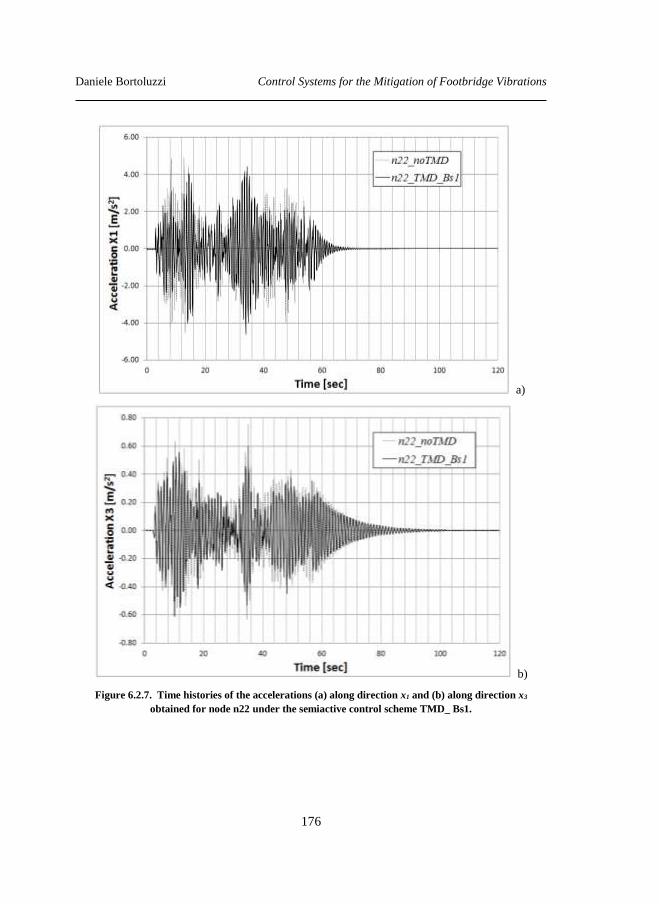
Daniele Bortoluzzi Control Systems for the Mitigation of Footbridge Vibrations
176
a)
b)
Figure 6.2.7. Time histories of the accelerations (a) along direction x1 and (b) along direction x3
obtained for node n22 under the semiactive control scheme TMD_ Bs1.
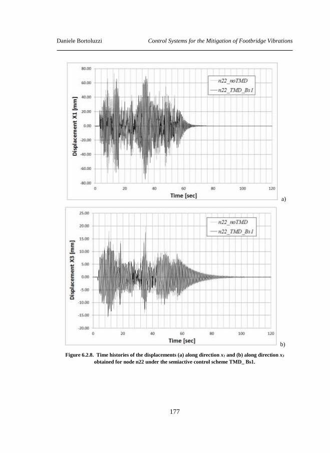
Daniele Bortoluzzi Control Systems for the Mitigation of Footbridge Vibrations
177
a)
b)
Figure 6.2.8. Time histories of the displacements (a) along direction x1 and (b) along direction x3
obtained for node n22 under the semiactive control scheme TMD_ Bs1.
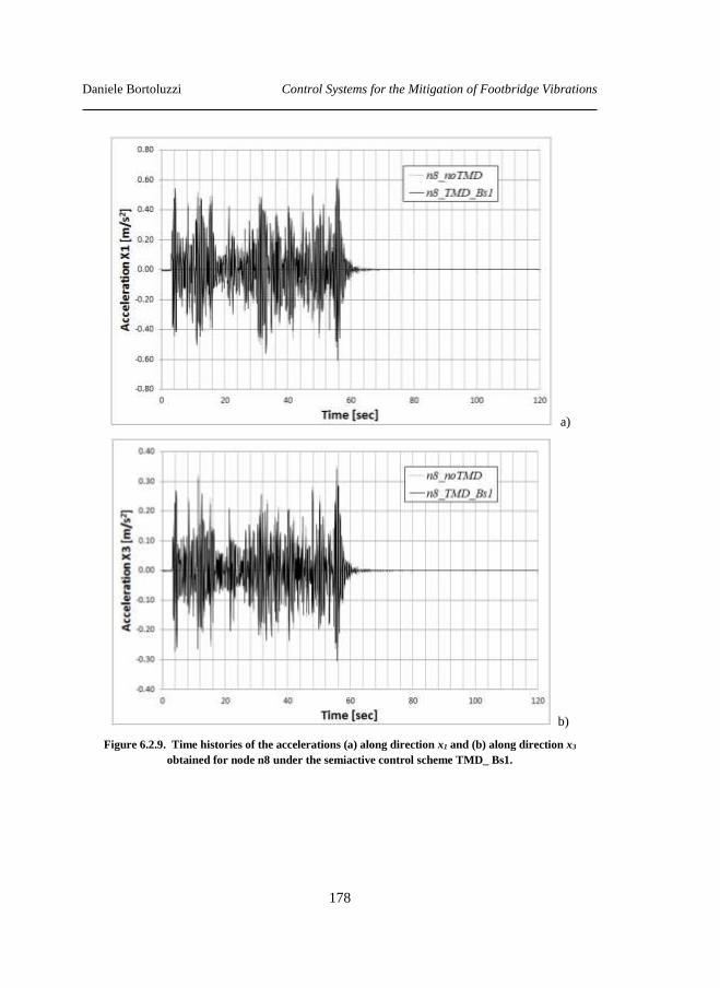
Daniele Bortoluzzi Control Systems for the Mitigation of Footbridge Vibrations
178
a)
b)
Figure 6.2.9. Time histories of the accelerations (a) along direction x1 and (b) along direction x3
obtained for node n8 under the semiactive control scheme TMD_ Bs1.
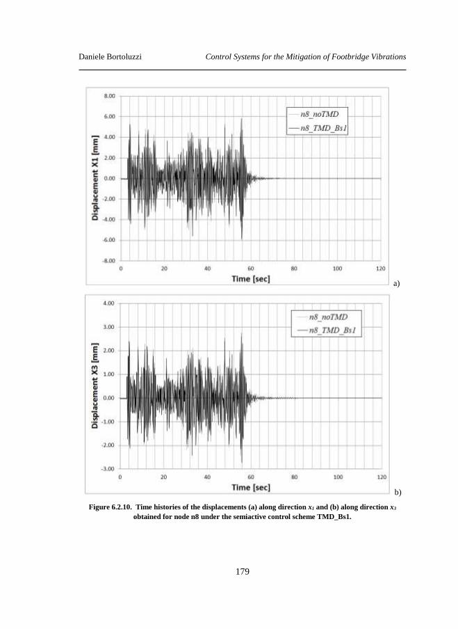
Daniele Bortoluzzi Control Systems for the Mitigation of Footbridge Vibrations
179
a)
b)
Figure 6.2.10. Time histories of the displacements (a) along direction x1 and (b) along direction x3
obtained for node n8 under the semiactive control scheme TMD_Bs1.
Daniele Bortoluzzi Control Systems for the Mitigation of Footbridge Vibrations
180
6.3 Active control solutions
Once achieved the reduction of the FEM for the “Trasaghis” footbridge (see section
5.2), a structural control is implemented within the MatLAB environment in order to
mitigate the vibration induced by wind loads (see section 5.2 and section 5.3).
The implemented active control strategy, or in other words the control forced introduced
within the model in order to achieve the purpose of the control, is based on the Linear
Quadratic Regulator (LQR) theory. This theory belong to the more general field of the
theory of optimal control that concern with the possibility to manage a given dynamic
system at its minimum “cost”. In all those cases where the dynamic of the system is
described by a set of linear differential equations and the cost may be described by a
quadratic function, a feedback control can be achieved by applying the LQR strategy as
follows described ([1] and [17]).
Let’s consider a linear dynamic system expressed in state variable form as:
x t x t u t A B , (6.13)
where x(t)∈Rn, u(t)∈Rm are respectively the states and input vectors, and the initial
conditions are assumed to be 0(0)x x .
The LQR strategy problem can be presented as follows: “find a state-variable feedback
(SVFB) control that gives desirable closed-loop properties, such that:”
u t x t v t K . (6.14)
where K is unknown matrix to be found and v(t) the new command input.
Substituting equation (6.14) in (6.13) the problem becomes:
Cx t x t v t x t v t A- BK B A B , (6.15)
where C A A - BK represents the closed-loop plant matrix.
It is reasonable now to design an optimal SVFB control. Thus, let’s introduce the
performance index (PI) as:
0
1
2
T TJ x x u u dt
Q R , (6.16)
Daniele Bortoluzzi Control Systems for the Mitigation of Footbridge Vibrations
181
where 1 0
0
n
ii
nn
Q
Q Q
Q
and , , 1,2,..., i ijr i j m R are the so called weighting
square diagonal matrices. The performance index J can be interpreted as an energy
function.
Since the only concerns are the internal stability properties of the closed-loop system, it
is reasonable to assume v(t) = 0. Thus, substituting equation (6.14) into (6.16) we
obtain:
0
1
2
T TJ x x dt Q K RK . (6.17)
Then the optimal SVFB design can be written as:
find K such that J=min(J); (6.18)
that is in other words, the optimal design concerns the search for the minimum of the
energy function J. Since the plant matrix is linear and the PI is quadratic, the problem to
minimize J is called the Linear Quadratic Regulator (LQR) where the word 'regulator'
refers to the fact that the function of this feedback is to regulate the states to zero (see
section 5.1). Depending on the parameters selected for the weighted matrices Q and R
during the design of the control law, the closed-loop system will exhibit a different
response.
It is important to observe that since x(t) and u(t) are weighted in J, in order to minimize
the function J neither x(t) nor u(t) can be too large. Note that if J is minimized, then it is
for sure finite quantity, and since by definition it is an infinite integral of x(t), then one
can said that x(t) goes to zero as time t goes to infinity. This in other words guarantees
that the closed-loop system will be stable.
Assuming that the closed-loop system is stable so that x(t) goes to zero as time t goes to
infinity, it can be shown as the function J is a constant that depends only on a new
auxiliary matrix P and the initial conditions, and it is independent from K. Then the
optimal feedback K can be evaluated as follows:
1 TK R B P , (6.19)
where P is a constant auxiliary matrix that can be evaluated solving the following
continuous time algebraic Riccati equation (ARE):
1 0T TA P + PA- PBR B P + Q = . (6.20)
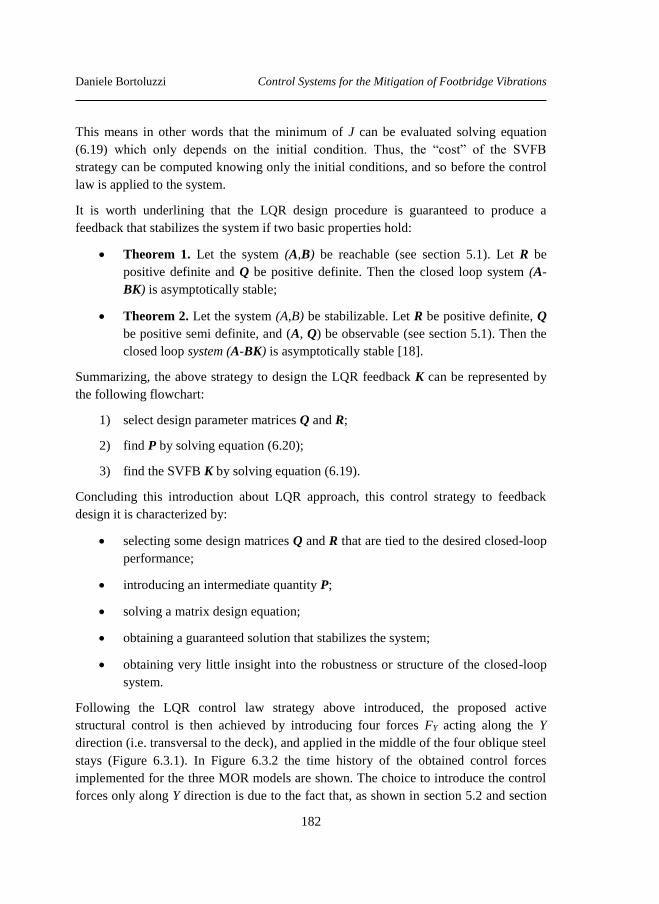
Daniele Bortoluzzi Control Systems for the Mitigation of Footbridge Vibrations
182
This means in other words that the minimum of J can be evaluated solving equation
(6.19) which only depends on the initial condition. Thus, the “cost” of the SVFB
strategy can be computed knowing only the initial conditions, and so before the control
law is applied to the system.
It is worth underlining that the LQR design procedure is guaranteed to produce a
feedback that stabilizes the system if two basic properties hold:
Theorem 1. Let the system (A,B) be reachable (see section 5.1). Let R be
positive definite and Q be positive definite. Then the closed loop system (A-
BK) is asymptotically stable;
Theorem 2. Let the system (A,B) be stabilizable. Let R be positive definite, Q
be positive semi definite, and (A, Q) be observable (see section 5.1). Then the
closed loop system (A-BK) is asymptotically stable [18].
Summarizing, the above strategy to design the LQR feedback K can be represented by
the following flowchart:
1) select design parameter matrices Q and R;
2) find P by solving equation (6.20);
3) find the SVFB K by solving equation (6.19).
Concluding this introduction about LQR approach, this control strategy to feedback
design it is characterized by:
selecting some design matrices Q and R that are tied to the desired closed-loop
performance;
introducing an intermediate quantity P;
solving a matrix design equation;
obtaining a guaranteed solution that stabilizes the system;
obtaining very little insight into the robustness or structure of the closed-loop
system.
Following the LQR control law strategy above introduced, the proposed active
structural control is then achieved by introducing four forces FY acting along the Y
direction (i.e. transversal to the deck), and applied in the middle of the four oblique steel
stays (Figure 6.3.1). In Figure 6.3.2 the time history of the obtained control forces
implemented for the three MOR models are shown. The choice to introduce the control
forces only along Y direction is due to the fact that, as shown in section 5.2 and section
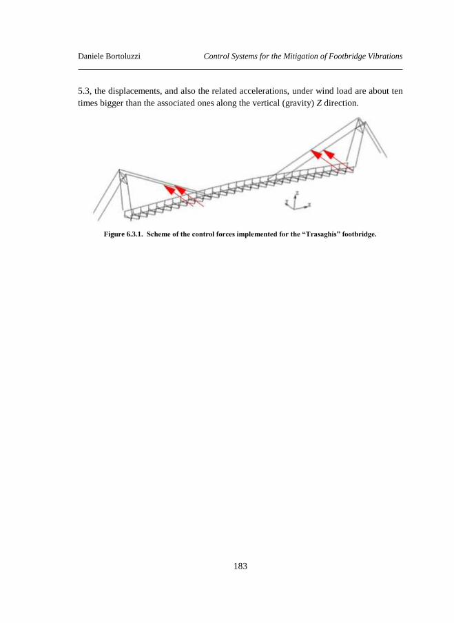
Daniele Bortoluzzi Control Systems for the Mitigation of Footbridge Vibrations
183
5.3, the displacements, and also the related accelerations, under wind load are about ten
times bigger than the associated ones along the vertical (gravity) Z direction.
Figure 6.3.1. Scheme of the control forces implemented for the “Trasaghis” footbridge.
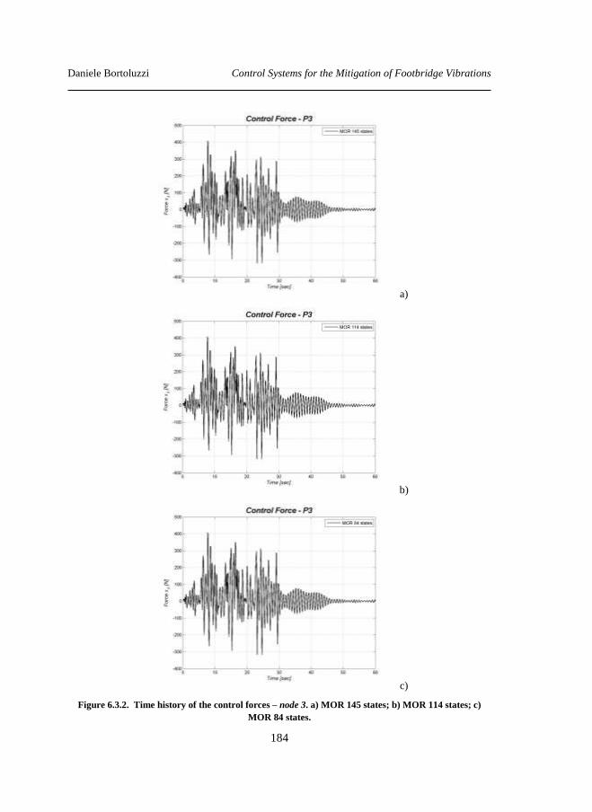
Daniele Bortoluzzi Control Systems for the Mitigation of Footbridge Vibrations
184
a)
b)
c)
Figure 6.3.2. Time history of the control forces – node 3. a) MOR 145 states; b) MOR 114 states; c)
MOR 84 states.
Daniele Bortoluzzi Control Systems for the Mitigation of Footbridge Vibrations
185
In the following figures (from Figure 6.3.3 to Figure 6.3.8) the results in terms of
displacements and accelerations along Y and Z axes for the case identified as
respectively “MOR 145 states”, “MOR 114 states” and “MOR 84 states”, obtained from
the above active control strategy, are compared with the related uncontrolled cases.
a)
b)
Figure 6.3.3. Active control solution for the “Trasaghis” footbridge - model MOR 145 states:
comparison of uncontrolled vs. controlled. Response of: a) Displacements along Y and Z axes – node 3;
b) Accelerations along Y and Z axes (zoom between 10 to 20 sec) – node 3.
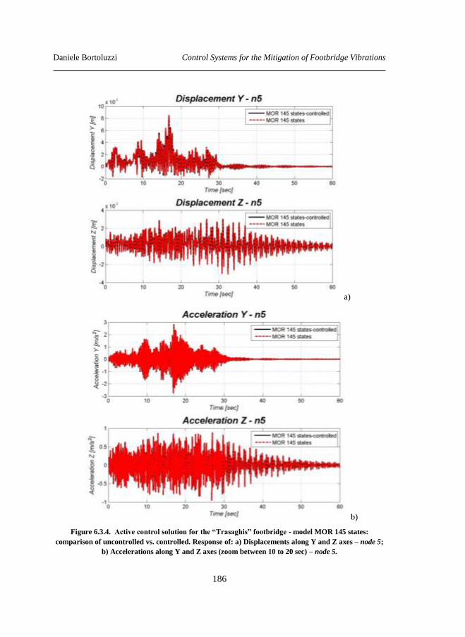
Daniele Bortoluzzi Control Systems for the Mitigation of Footbridge Vibrations
186
a)
b)
Figure 6.3.4. Active control solution for the “Trasaghis” footbridge - model MOR 145 states:
comparison of uncontrolled vs. controlled. Response of: a) Displacements along Y and Z axes – node 5;
b) Accelerations along Y and Z axes (zoom between 10 to 20 sec) – node 5.
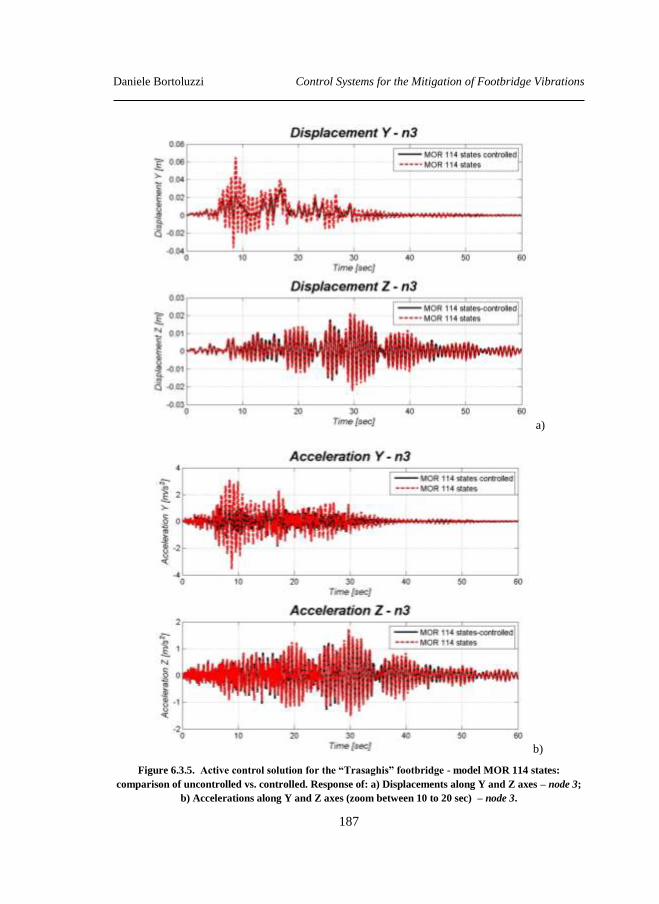
Daniele Bortoluzzi Control Systems for the Mitigation of Footbridge Vibrations
187
a)
b)
Figure 6.3.5. Active control solution for the “Trasaghis” footbridge - model MOR 114 states:
comparison of uncontrolled vs. controlled. Response of: a) Displacements along Y and Z axes – node 3;
b) Accelerations along Y and Z axes (zoom between 10 to 20 sec) – node 3.
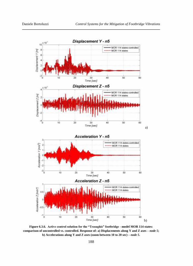
Daniele Bortoluzzi Control Systems for the Mitigation of Footbridge Vibrations
188
a)
b)
Figure 6.3.6. Active control solution for the “Trasaghis” footbridge - model MOR 114 states:
comparison of uncontrolled vs. controlled. Response of: a) Displacements along Y and Z axes – node 5;
b) Accelerations along Y and Z axes (zoom between 10 to 20 sec) – node 5.
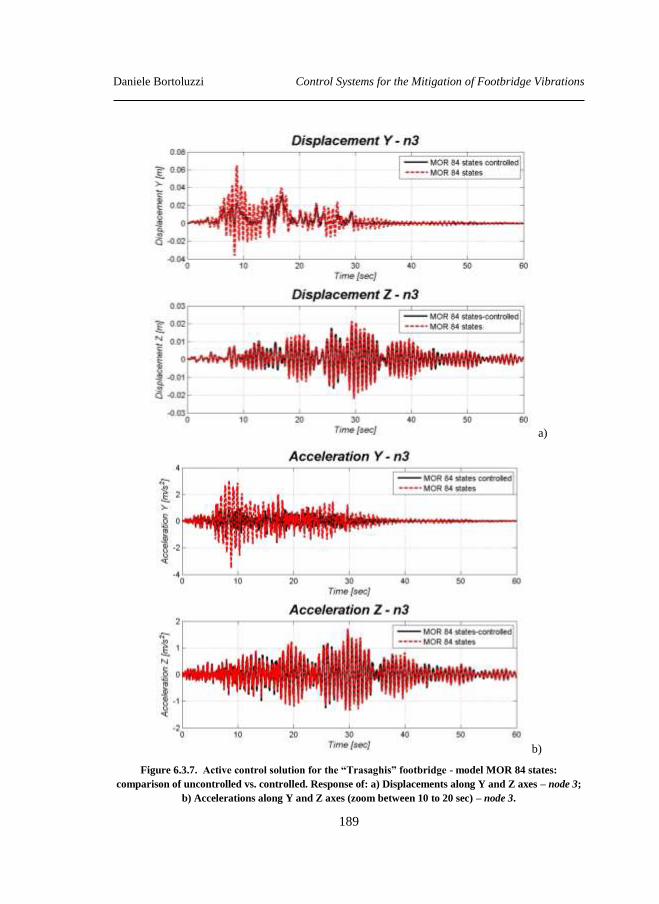
Daniele Bortoluzzi Control Systems for the Mitigation of Footbridge Vibrations
189
a)
b)
Figure 6.3.7. Active control solution for the “Trasaghis” footbridge - model MOR 84 states:
comparison of uncontrolled vs. controlled. Response of: a) Displacements along Y and Z axes – node 3;
b) Accelerations along Y and Z axes (zoom between 10 to 20 sec) – node 3.

Daniele Bortoluzzi Control Systems for the Mitigation of Footbridge Vibrations
190
a)
b)
Figure 6.3.8. Active control solution for the “Trasaghis” footbridge - model MOR 84 states:
comparison of uncontrolled vs. controlled. Response of: a) Displacements along Y and Z axes – node 5;
b) Accelerations along Y and Z axes (zoom between 10 to 20 sec) – node 5.
Daniele Bortoluzzi Control Systems for the Mitigation of Footbridge Vibrations
191
Concluding, the active proposed structural control implemented for the wind vibration
control of the “Trasaghis” footbridge seems to be consistent in terms both of quality and
quantity of the vibrations reduction. The better results, due to the design choices about
the control forces, are achieved for the reduction of the vibration along the transversal Y
axis; while small advantage seems to appear along Z direction. Moreover the results
shown, as expected, that the implementation of an active control solution allows to
achieve better results in terms of vibrations mitigation compared with the other
solutions previously analyzed [19].
6.4 References
[1] Chu, S.Y.; Soong, T.T.; Reinhorn, A.M., 2005. Active, Hybrid and Semi-
Active Structural Control. John Wiley & Sons. ISBN 0-470-01352-4.
[2] Soong T.T., Dargush G.F., 2007. Passive Energy Dissipation Systems in
Structural Engineering, John Wiley & Sons, Chichester, UK.
[3] Bursi, O. S. , Bonelli A., Ceravolo R., Tondini N., Ussia A., 2011. Dynamic
and Aeroelastic Behavior of a Twin Deck Curved Cable-Stayed Footbridge
Equipped with Passive Devices. On the Proceedings of the Engineering
Mechanics Institute 2011 Conference EMI 2011, Boston, USA, June 2-4, 2011,
366-379.
[4] A. Tributsch and C. Adam, 2012. Evaluation and analytical approximation of
Tuned Mass Damper performance in an earthquake environment. Smart
Structures and Systems, Vol. 10, No. 2 (2012) 155-179.
[5] Schmelzer, B., Oberguggenberger, M., Adam, C., 2010. Performance of Tuned
Mass Dampers with uncertain parameters under stochastic excitation. On the
Proceedings of the Institution of Mechanical Engineers, Part O: Journal of Risk
and Reliability, 224, 4, pp. 298 - 308.
[6] Ussia A.,Bursi, O. S. , Bonelli A., 2012. Optimal Semi Active MR Control
Strategies of a Footbridge Endowed with TMDs, smart structures, On the
Proceedings of the 5th European Conference on Structural Control, EACS
2012, Genoa, Italy, June 18-20, 2012.
[7] Casciati F. and Giuliano F., 2009. Performance of Multi-TMD in the Towers
of Suspension Bridges, Journal of Vibration and Control, 15 (6), pp. 821-847.
[8] Rana R. and Soong T.T., 1998. Parametric study and simplified design of
tuned mass dampers, Engineering Structures, 20, pp. 193-204.
Daniele Bortoluzzi Control Systems for the Mitigation of Footbridge Vibrations
192
[9] Abe, M. and Fujino, Y., 1994. Dynamic Characterization of Multiple Tuned
Mass Dampers and Some Design Formulas. Earthquake Engineering and
Structural Dynamics, 23, pp. 813-835.
[10] Abe, M. and Igusa, T., 1995. Tuned Mass Dampers with Closely Spaced
Natural Frequencies. Earthquake Engineering and Structural Dynamics, 24 ,
pp. 247-261.
[11] Bandivadekar T.P, Jangid R.S., 2012. Mass distribution of multiple tuned mass
dampers for vibration control of Structures. International Journal Of Civil And
Structural Engineering, 3 (1).
[12] www.mathworks.it
[13] NTC 2008. Norme tecniche per le costruzioni (in Italian) - D.M. 14 Gennaio
2008.
[14] www.mscsoftware.com
[15] Warburton, G. B., 1982. Optimal Absorber Parameters for Various
Combinations of Response and Excitation Parameters. Earthquake Engineering
and Structural Dynamics, Vol. 10, pp. 381-401.
[16] Casciati F, Magonette G. and Marazzi F., 2007. Technology of Semiactive
Devices and Applications in Vibration Mitigation, John Wiley & Sons,
Chichester, UK.
[17] A. Preumont, 2004. Vibration Control of Active Structures. An Introduction,
2nd edition. Kluwer Academic Publishers. New York, Boston, Dordrecht,
London, Moscow. ISBN: 1-4020-0496-6.
[18] Schilders W.H.A., van der Vorst H.A., Rommes J. 2008. Model Order
Reduction: Theory, Research Aspects and Applications, Springer.
[19] C.M. Casado, I.M. Diaz, J. de Sebastian, A.V. Poncela and A. Lorenzana,
Implementation of Passive and Active Vibration Control on an In-service
Footbridge, Structural Control and Health Monitoring, 20,2013, pp. 70-87.

Daniele Bortoluzzi Control Systems for the Mitigation of Footbridge Vibrations
193
Chapter 7 Conclusions
In this thesis some control solutions for the vibrations mitigation of pedestrian timber
bridges are studied and analyzed.
The main motivations of this thesis are:
1) the research in this field is still in progress and several researches all around
the world are addressing the study of comfort problems, vibrations control, and
so forth… in the area of pedestrian bridges;
2) the design process of the footbridge should include the effects of the so called
Human Induced Loads (HIL) which are presently under investigation in view
of an accurate modelling.
After a state of the art focused on contributions to international conferences held in
2014 on this theme and on existing codes and recommendations, two chapters are
devoted to the numerical modelling of the structural system and of the actions,
respectively.
Model Order Reduction is discussed in the fifth chapter, while the last chapter before
these conclusions summarises the proposed passive and active control solutions
conceived and designed within this work of thesis.
Two case studies have supported the numerical investigations. Their importance relies
on the fact that those structural systems were fully identified by “in situ” experimental
campaigns, designed and carried out by the author. Those structural systems were
designed respectful of a structural code which only prescribes a static design for them.
As a result control schemes are quite desirable in view of ensuring (enhancing) the
comfort of the crossing persons (serviceability limit state).
In this thesis, however, there is also an effort to build a design procedure accounting for
the induced vibrations which should be able to avoid control correction once the
footbridge is put in service.

Daniele Bortoluzzi Control Systems for the Mitigation of Footbridge Vibrations
194
Daniele Bortoluzzi Control Systems for the Mitigation of Footbridge Vibrations
195
Appendix A: Technical details for the two footbridges used
as case studies
In this chapter some technical details concerning the two footbridges used as case
studies are discussed. In particular information on dimensions, materials, constructions
techniques and stages, and so forth…are summarized.
In the first section the pedestrian bridge located, in the Trasaghis Municipality and
labelled as “Trasaghis footbridge”, is reported. In the second session the pedestrian
bridge, located in Farra d’Alpago Municipality and labelled as “Tesa footbridge”, is
discussed.
A.1 Trasaghis footbridge
In the North-Eastern Italian region of Friuli, there is a mountain area (Gemona
Municipality) which became world-wide famous in 1976 when shaken by a strong
earthquake in the spring. The event was followed by a further significant shake in the
late summer of the same year. Nevertheless, that area recovered from those catastrophic
events and its economy is now strong with an important source coming from the
tourism.
The local largest natural lake is called the “Lake of the three municipalities” (or the
“Cavazzo Lake” – see the red circle in Figure A.1.1) with an emissary channel which
was a barrier for the jogging activity across the surrounding park.
Thus, the designer in accordance with the owner authority, decided to link the two side
of the outlet channel with a pedestrian bridge (Figure A.1.2). In particular, for both
economical and environmental reasons, only eco-friendly materials (i.e. steel and
timber) were adopted to harmonize the structure with the surrounding environment.
Indeed, as explained later on, the use of reinforced concrete was limited only to the
foundation components.
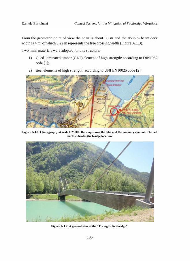
Daniele Bortoluzzi Control Systems for the Mitigation of Footbridge Vibrations
196
From the geometric point of view the span is about 83 m and the double- beam deck
width is 4 m, of which 3.22 m represents the free crossing width (Figure A.1.3).
Two main materials were adopted for this structure:
1) glued laminated timber (GLT) element of high strength: according to DIN1052
code [1];
2) steel elements of high strength: according to UNI EN10025 code [2].
Figure A.1.1. Chorography at scale 1:25000: the map shows the lake and the emissary channel. The red
circle indicates the bridge location.
Figure A.1.2. A general view of the “Trasaghis footbridge”.
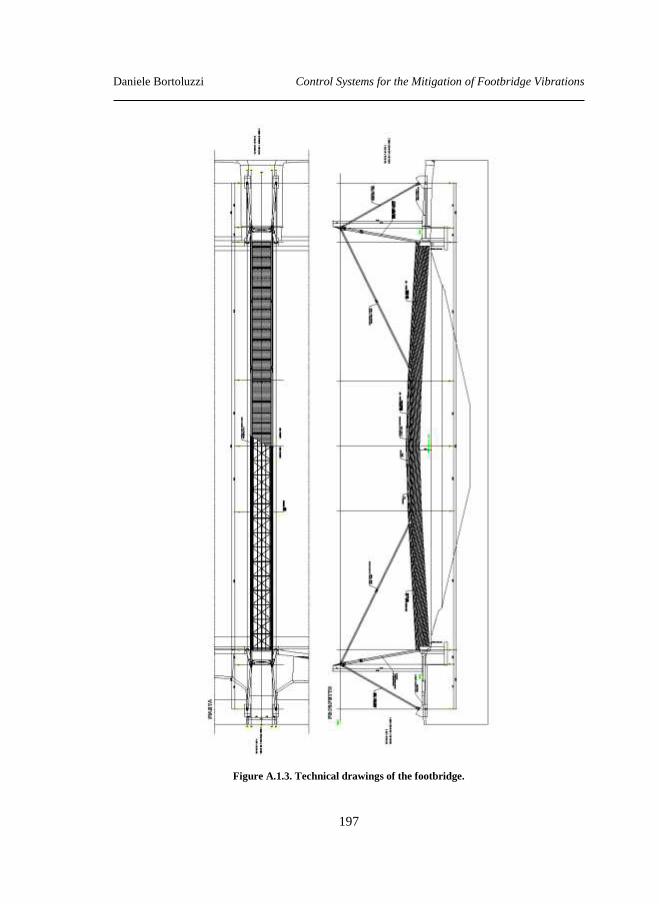
Daniele Bortoluzzi Control Systems for the Mitigation of Footbridge Vibrations
197
Figure A.1.3. Technical drawings of the footbridge.
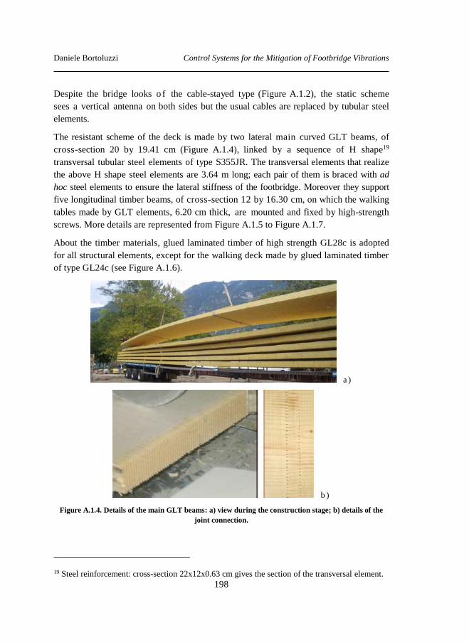
Daniele Bortoluzzi Control Systems for the Mitigation of Footbridge Vibrations
198
Despite the bridge looks o f the cable-stayed type (Figure A.1.2), the static scheme
sees a vertical antenna on both sides but the usual cables are replaced by tubular steel
elements.
The resistant scheme of the deck is made by two lateral main curved GLT beams, of
cross-section 20 by 19.41 cm (Figure A.1.4), linked by a sequence of H shape19
transversal tubular steel elements of type S355JR. The transversal elements that realize
the above H shape steel elements are 3.64 m long; each pair of them is braced with ad
hoc steel elements to ensure the lateral stiffness of the footbridge. Moreover they support
five longitudinal timber beams, of cross-section 12 by 16.30 cm, on which the walking
tables made by GLT elements, 6.20 cm thick, are mounted and fixed by high-strength
screws. More details are represented from Figure A.1.5 to Figure A.1.7.
About the timber materials, glued laminated timber of high strength GL28c is adopted
for all structural elements, except for the walking deck made by glued laminated timber
of type GL24c (see Figure A.1.6).
a )
b )
Figure A.1.4. Details of the main GLT beams: a) view during the construction stage; b) details of the
joint connection.
19 Steel reinforcement: cross-section 22x12x0.63 cm gives the section of the transversal element.
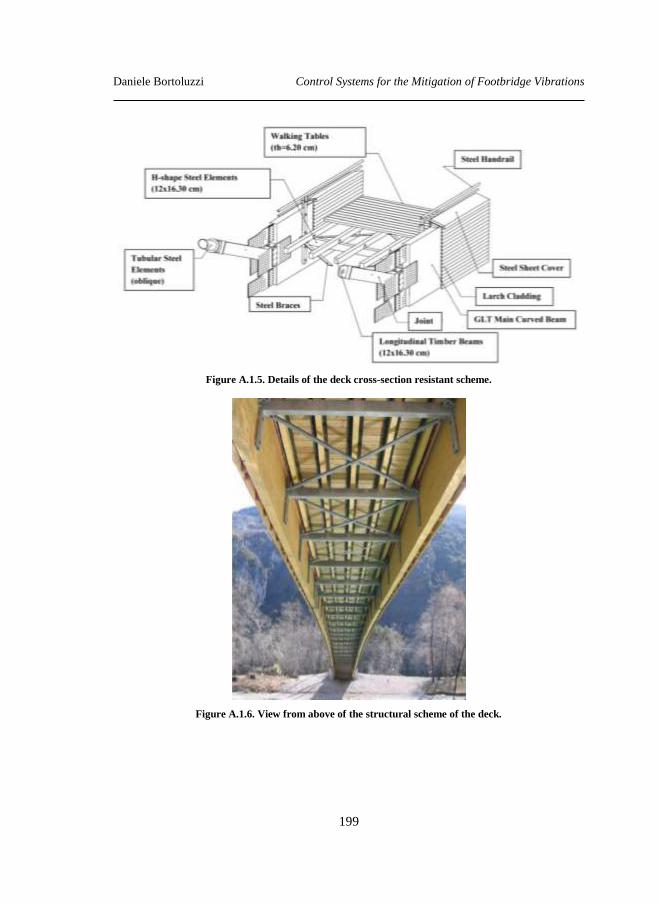
Daniele Bortoluzzi Control Systems for the Mitigation of Footbridge Vibrations
199
Figure A.1.5. Details of the deck cross-section resistant scheme.
Figure A.1.6. View from above of the structural scheme of the deck.
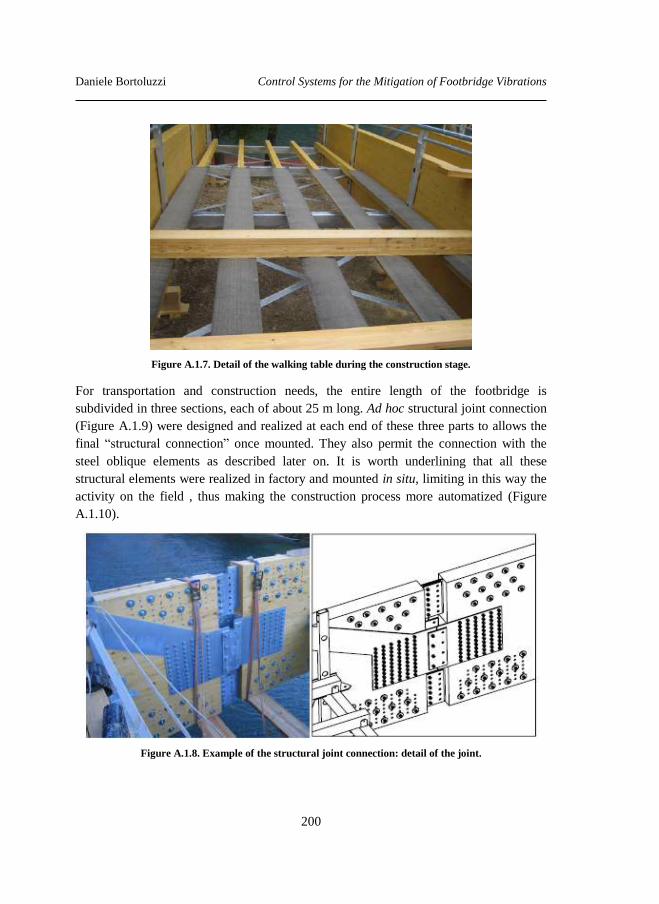
Daniele Bortoluzzi Control Systems for the Mitigation of Footbridge Vibrations
200
Figure A.1.7. Detail of the walking table during the construction stage.
For transportation and construction needs, the entire length of the footbridge is
subdivided in three sections, each of about 25 m long. Ad hoc structural joint connection
(Figure A.1.9) were designed and realized at each end of these three parts to allows the
final “structural connection” once mounted. They also permit the connection with the
steel oblique elements as described later on. It is worth underlining that all these
structural elements were realized in factory and mounted in situ, limiting in this way the
activity on the field , thus making the construction process more automatized (Figure
A.1.10).
Figure A.1.8. Example of the structural joint connection: detail of the joint.
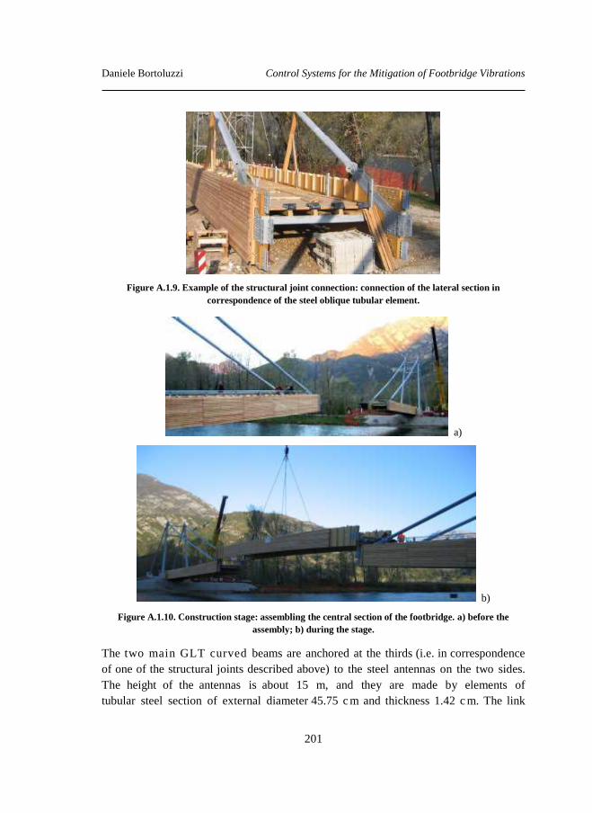
Daniele Bortoluzzi Control Systems for the Mitigation of Footbridge Vibrations
201
Figure A.1.9. Example of the structural joint connection: connection of the lateral section in
correspondence of the steel oblique tubular element.
a)
b)
Figure A.1.10. Construction stage: assembling the central section of the footbridge. a) before the
assembly; b) during the stage.
The two main GLT curved beams are anchored at the thirds (i.e. in correspondence
of one of the structural joints described above) to the steel antennas on the two sides.
The height of the antennas is about 15 m, and they are made by elements of
tubular steel section of external diameter 45.75 c m and thickness 1.42 c m. The link
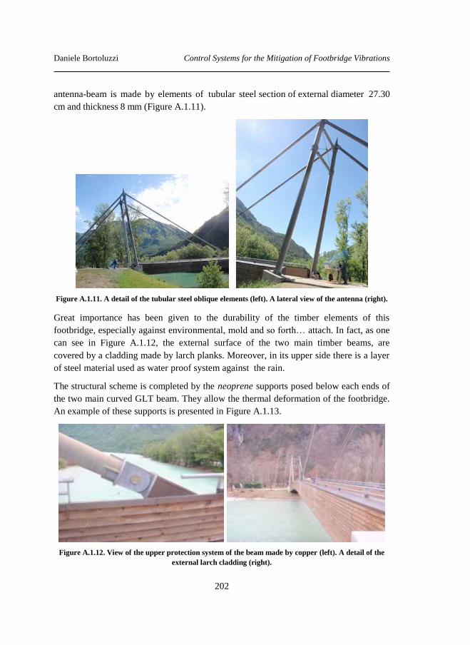
Daniele Bortoluzzi Control Systems for the Mitigation of Footbridge Vibrations
202
antenna-beam is made by elements of tubular steel section of external diameter 27.30
cm and thickness 8 mm (Figure A.1.11).
Figure A.1.11. A detail of the tubular steel oblique elements (left). A lateral view of the antenna (right).
Great importance has been given to the durability of the timber elements of this
footbridge, especially against environmental, mold and so forth… attach. In fact, as one
can see in Figure A.1.12, the external surface of the two main timber beams, are
covered by a cladding made by larch planks. Moreover, in its upper side there is a layer
of steel material used as water proof system against the rain.
The structural scheme is completed by the neoprene supports posed below each ends of
the two main curved GLT beam. They allow the thermal deformation of the footbridge.
An example of these supports is presented in Figure A.1.13.
Figure A.1.12. View of the upper protection system of the beam made by copper (left). A detail of the
external larch cladding (right).

Daniele Bortoluzzi Control Systems for the Mitigation of Footbridge Vibrations
203
Figure A.1.13. View of the neoprene support.
From the prescriptive point of view, the pedestrian bridge is regarded as category 3
according with the Italian code [3]-[4]. This means that during the design stage beyond
the usual “dead” loads, other two “live” loads have to be considered in a static
configuration; in particular:
1) q1.d = isolated load of 10 kN over an area of 70 by 70 cm;
2) q1.e = distributed load of 4.0 kN/m2 resulting from a dense people gathering.
In addition20 to the above loads, the effects of snow, wind and earthquake were taken
into account by the designer.
Once finished the construction stage, the static proof test required by the Italian
regulation [3]-[4] was carried out. In addition to the dead loads due to the structural and
non-structural elements of the footbridge, an additional loads provided by ad hoc
devices was added (Figure A.1.14) up to the value suggested by the regulation: q1.e =
4.0 kN/m2. Once loaded the deck, the measurement of the vertical displacement of
sensitive points along the footbridge due to the above loads (Figure A.1.15) was carried
out. The maximum vertical displacement measured in the middle of the span was 14.5
cm.
20 It is worth noting that for this structure no particular analysis/assessment of comfort was
required during the design stage.

Daniele Bortoluzzi Control Systems for the Mitigation of Footbridge Vibrations
204
a)
b)
Figure A.1.14. Load test stage. a) Load configuration (measure in m); b) during the test (below).
Figure A.1.15. Measurement during the load test stage carried out.
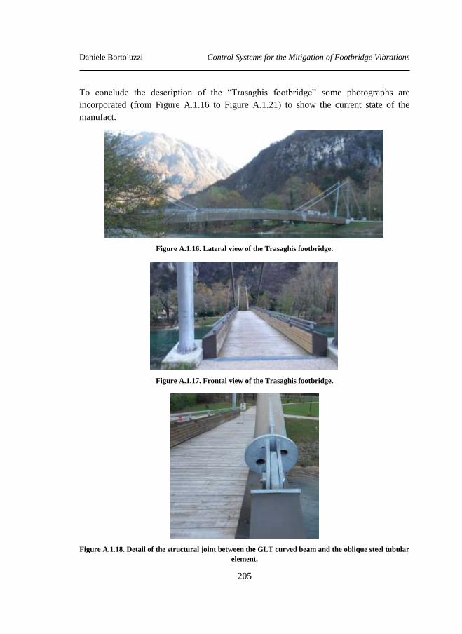
Daniele Bortoluzzi Control Systems for the Mitigation of Footbridge Vibrations
205
To conclude the description of the “Trasaghis footbridge” some photographs are
incorporated (from Figure A.1.16 to Figure A.1.21) to show the current state of the
manufact.
Figure A.1.16. Lateral view of the Trasaghis footbridge.
Figure A.1.17. Frontal view of the Trasaghis footbridge.
Figure A.1.18. Detail of the structural joint between the GLT curved beam and the oblique steel tubular
element.
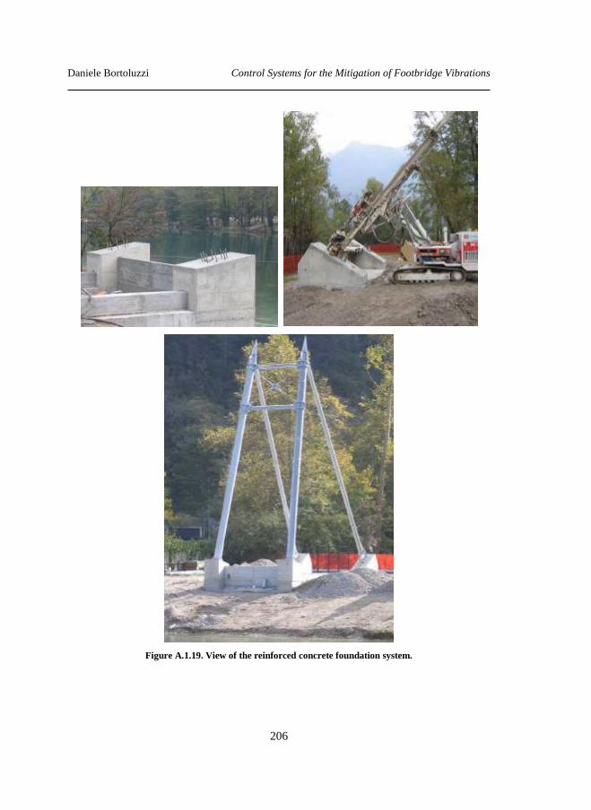
Daniele Bortoluzzi Control Systems for the Mitigation of Footbridge Vibrations
206
Figure A.1.19. View of the reinforced concrete foundation system.
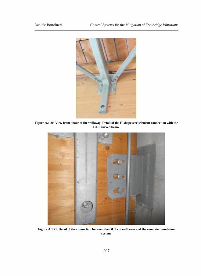
Daniele Bortoluzzi Control Systems for the Mitigation of Footbridge Vibrations
207
Figure A.1.20. View from above of the walkway. Detail of the H-shape steel element connection with the
GLT curved beam.
Figure A.1.21. Detail of the connection between the GLT curved beam and the concrete foundation
system.
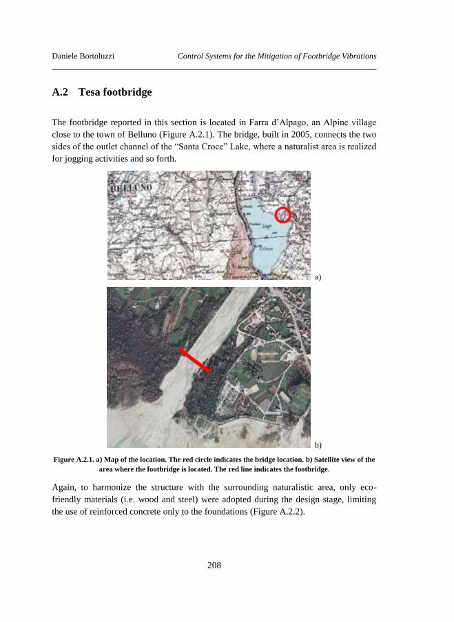
Daniele Bortoluzzi Control Systems for the Mitigation of Footbridge Vibrations
208
A.2 Tesa footbridge
The footbridge reported in this section is located in Farra d’Alpago, an Alpine village
close to the town of Belluno (Figure A.2.1). The bridge, built in 2005, connects the two
sides of the outlet channel of the “Santa Croce” Lake, where a naturalist area is realized
for jogging activities and so forth.
a)
b)
Figure A.2.1. a) Map of the location. The red circle indicates the bridge location. b) Satellite view of the
area where the footbridge is located. The red line indicates the footbridge.
Again, to harmonize the structure with the surrounding naturalistic area, only eco-
friendly materials (i.e. wood and steel) were adopted during the design stage, limiting
the use of reinforced concrete only to the foundations (Figure A.2.2).
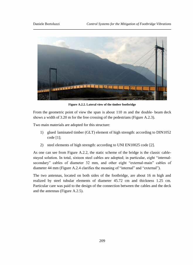
Daniele Bortoluzzi Control Systems for the Mitigation of Footbridge Vibrations
209
Figure A.2.2. Lateral view of the timber footbridge
From the geometric point of view the span is about 110 m and the double- beam deck
shows a width of 3.20 m for the free crossing of the pedestrians (Figure A.2.3).
Two main materials are adopted for this structure:
1) glued laminated timber (GLT) element of high strength: according to DIN1052
code [1];
2) steel elements of high strength: according to UNI EN10025 code [2].
As one can see from Figure A.2.2, the static scheme of the bridge is the classic cable-
stayed solution. In total, sixteen steel cables are adopted; in particular, eight “internal-
secondary” cables of diameter 32 mm, and other eight “external-main” cables of
diameter 44 mm (Figure A.2.4 clarifies the meaning of “internal” and “external”).
The two antennas, located on both sides of the footbridge, are about 16 m high and
realized by steel tubular elements of diameter 45.72 cm and thickness 1.25 cm.
Particular care was paid to the design of the connection between the cables and the deck
and the antennas (Figure A.2.5).
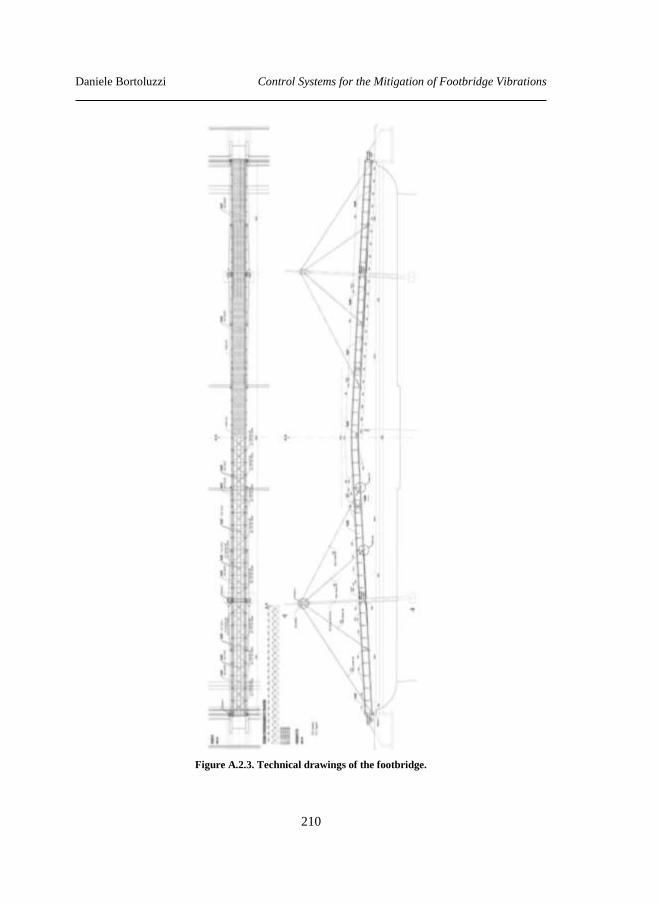
Daniele Bortoluzzi Control Systems for the Mitigation of Footbridge Vibrations
210
Figure A.2.3. Technical drawings of the footbridge.
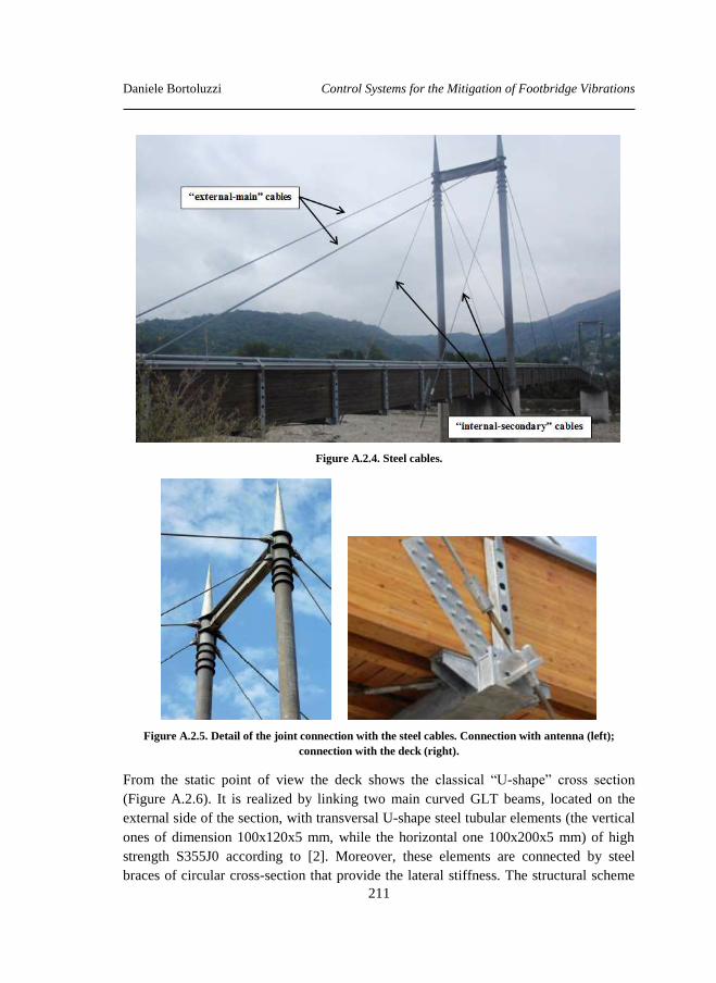
Daniele Bortoluzzi Control Systems for the Mitigation of Footbridge Vibrations
211
Figure A.2.4. Steel cables.
Figure A.2.5. Detail of the joint connection with the steel cables. Connection with antenna (left);
connection with the deck (right).
From the static point of view the deck shows the classical “U-shape” cross section
(Figure A.2.6). It is realized by linking two main curved GLT beams, located on the
external side of the section, with transversal U-shape steel tubular elements (the vertical
ones of dimension 100x120x5 mm, while the horizontal one 100x200x5 mm) of high
strength S355J0 according to [2]. Moreover, these elements are connected by steel
braces of circular cross-section that provide the lateral stiffness. The structural scheme
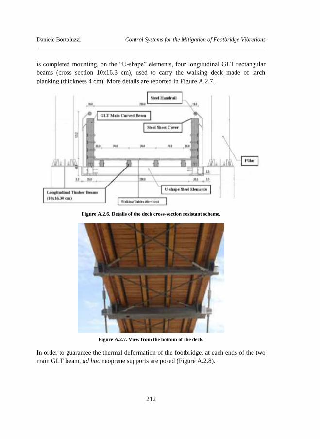
Daniele Bortoluzzi Control Systems for the Mitigation of Footbridge Vibrations
212
is completed mounting, on the “U-shape” elements, four longitudinal GLT rectangular
beams (cross section 10x16.3 cm), used to carry the walking deck made of larch
planking (thickness 4 cm). More details are reported in Figure A.2.7.
Figure A.2.6. Details of the deck cross-section resistant scheme.
Figure A.2.7. View from the bottom of the deck.
In order to guarantee the thermal deformation of the footbridge, at each ends of the two
main GLT beam, ad hoc neoprene supports are posed (Figure A.2.8).
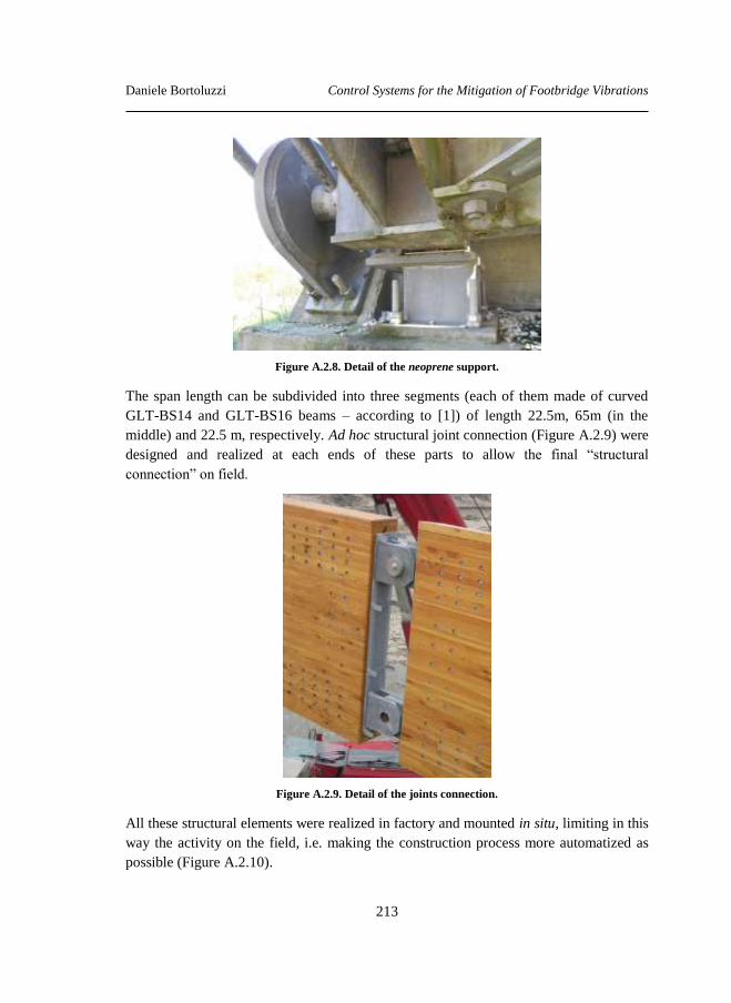
Daniele Bortoluzzi Control Systems for the Mitigation of Footbridge Vibrations
213
Figure A.2.8. Detail of the neoprene support.
The span length can be subdivided into three segments (each of them made of curved
GLT-BS14 and GLT-BS16 beams – according to [1]) of length 22.5m, 65m (in the
middle) and 22.5 m, respectively. Ad hoc structural joint connection (Figure A.2.9) were
designed and realized at each ends of these parts to allow the final “structural
connection” on field.
Figure A.2.9. Detail of the joints connection.
All these structural elements were realized in factory and mounted in situ, limiting in this
way the activity on the field, i.e. making the construction process more automatized as
possible (Figure A.2.10).
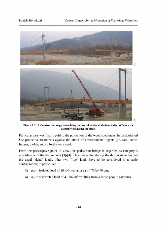
Daniele Bortoluzzi Control Systems for the Mitigation of Footbridge Vibrations
214
a)
b)
Figure A.2.10. Construction stage: assembling the central section of the footbridge. a) Before the
assembly; b) during the stage.
Particular care was finally paid to the protection of the wood specimens; in particular ad
hoc protective treatments against the attack of environmental agents (i.e. rain, snow,
fungus, molds, and so forth) were used.
From the prescriptive point of view, the pedestrian bridge is regarded as category 3
according with the Italian code [3]-[4]. This means that during the design stage beyond
the usual “dead” loads, other two “live” loads have to be considered in a static
configuration; in particular:
3) q1.d = isolated load of 10 kN over an area of 70 by 70 cm;
4) q1.e = distributed load of 4.0 kN/m2 resulting from a dense people gathering.
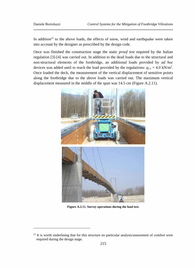
Daniele Bortoluzzi Control Systems for the Mitigation of Footbridge Vibrations
215
In addition21 to the above loads, the effects of snow, wind and earthquake were taken
into account by the designer as prescribed by the design code.
Once was finished the construction stage the static proof test required by the Italian
regulation [3]-[4] was carried out. In addition to the dead loads due to the structural and
non-structural elements of the footbridge, an additional loads provided by ad hoc
devices was added until to reach the load provided by the regulations: q1.e = 4.0 kN/m2.
Once loaded the deck, the measurement of the vertical displacement of sensitive points
along the footbridge due to the above loads was carried out. The maximum vertical
displacement measured in the middle of the span was 14.5 cm (Figure A.2.11).
Figure A.2.11. Survey operations during the load test.
21 It is worth underlining that for this structure no particular analysis/assessment of comfort were
required during the design stage.
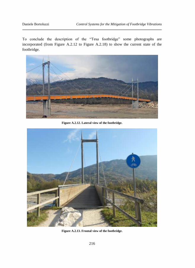
Daniele Bortoluzzi Control Systems for the Mitigation of Footbridge Vibrations
216
To conclude the description of the “Tesa footbridge” some photographs are
incorporated (from Figure A.2.12 to Figure A.2.18) to show the current state of the
footbridge.
Figure A.2.12. Lateral view of the footbridge.
Figure A.2.13. Frontal view of the footbridge.
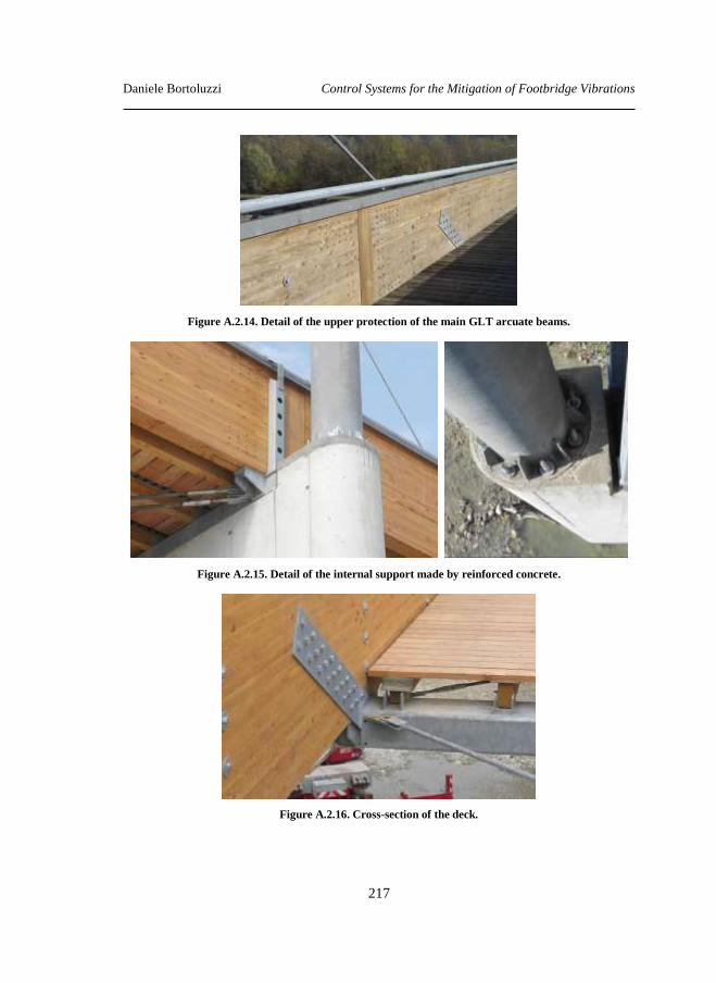
Daniele Bortoluzzi Control Systems for the Mitigation of Footbridge Vibrations
217
Figure A.2.14. Detail of the upper protection of the main GLT arcuate beams.
Figure A.2.15. Detail of the internal support made by reinforced concrete.
Figure A.2.16. Cross-section of the deck.
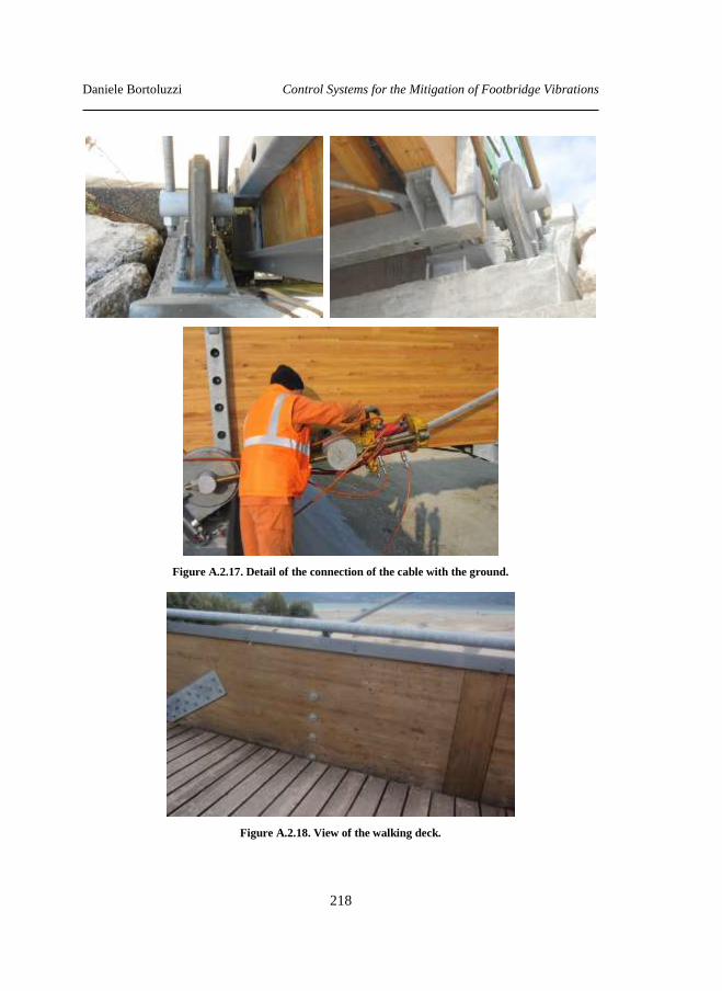
Daniele Bortoluzzi Control Systems for the Mitigation of Footbridge Vibrations
218
Figure A.2.17. Detail of the connection of the cable with the ground.
Figure A.2.18. View of the walking deck.

Daniele Bortoluzzi Control Systems for the Mitigation of Footbridge Vibrations
219
A.3 References
[1] DIN 1052: Design, Analysis and design of timber structures
[2] UNI EN 10025: Hot rolled products of non-alloy steel for structural
applications. Technical delivery conditions.
[3] D.M. 16 gennaio 1996 – Norme tecniche per le costruzioni in zona sismica [In
Italian].
[4] Norme tecniche per le costruzioni - D.M. 14 Gennaio 2008 (NTC2008) [In
Italian].

Daniele Bortoluzzi Control Systems for the Mitigation of Footbridge Vibrations
220
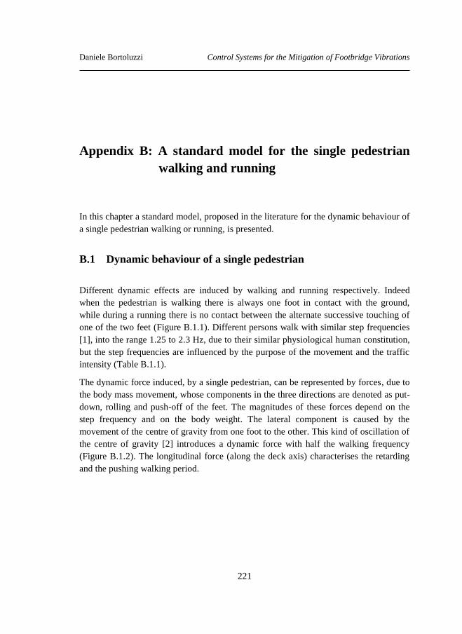
Daniele Bortoluzzi Control Systems for the Mitigation of Footbridge Vibrations
221
Appendix B: A standard model for the single pedestrian
walking and running
In this chapter a standard model, proposed in the literature for the dynamic behaviour of
a single pedestrian walking or running, is presented.
B.1 Dynamic behaviour of a single pedestrian
Different dynamic effects are induced by walking and running respectively. Indeed
when the pedestrian is walking there is always one foot in contact with the ground,
while during a running there is no contact between the alternate successive touching of
one of the two feet (Figure B.1.1). Different persons walk with similar step frequencies
[1], into the range 1.25 to 2.3 Hz, due to their similar physiological human constitution,
but the step frequencies are influenced by the purpose of the movement and the traffic
intensity (Table B.1.1).
The dynamic force induced, by a single pedestrian, can be represented by forces, due to
the body mass movement, whose components in the three directions are denoted as put-
down, rolling and push-off of the feet. The magnitudes of these forces depend on the
step frequency and on the body weight. The lateral component is caused by the
movement of the centre of gravity from one foot to the other. This kind of oscillation of
the centre of gravity [2] introduces a dynamic force with half the walking frequency
(Figure B.1.2). The longitudinal force (along the deck axis) characterises the retarding
and the pushing walking period.
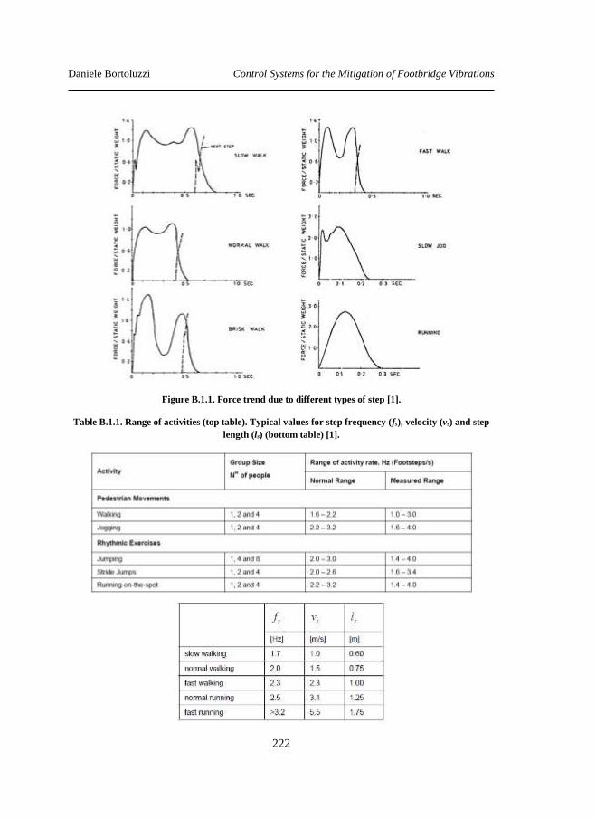
Daniele Bortoluzzi Control Systems for the Mitigation of Footbridge Vibrations
222
Figure B.1.1. Force trend due to different types of step [1].
Table B.1.1. Range of activities (top table). Typical values for step frequency (fs), velocity (vs) and step
length (ls) (bottom table) [1].
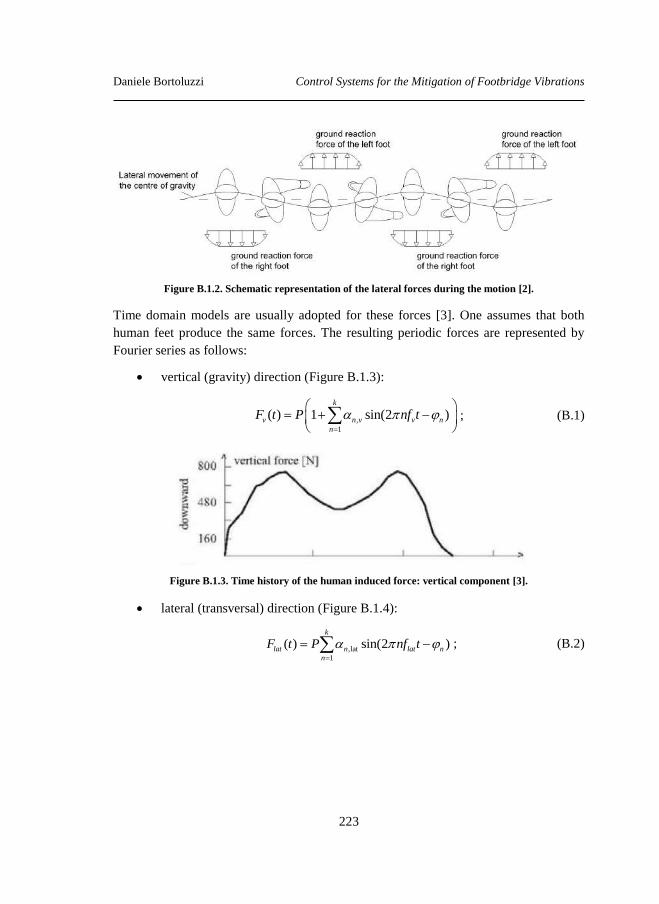
Daniele Bortoluzzi Control Systems for the Mitigation of Footbridge Vibrations
223
Figure B.1.2. Schematic representation of the lateral forces during the motion [2].
Time domain models are usually adopted for these forces [3]. One assumes that both
human feet produce the same forces. The resulting periodic forces are represented by
Fourier series as follows:
vertical (gravity) direction (Figure B.1.3):
; (B.1)
Figure B.1.3. Time history of the human induced force: vertical component [3].
lateral (transversal) direction (Figure B.1.4):
; (B.2)
,
1
( ) 1 sin(2 )k
v n v v n
n
F t P nf t
,lat
1
( ) sin(2 )k
lat n lat n
n
F t P nf t
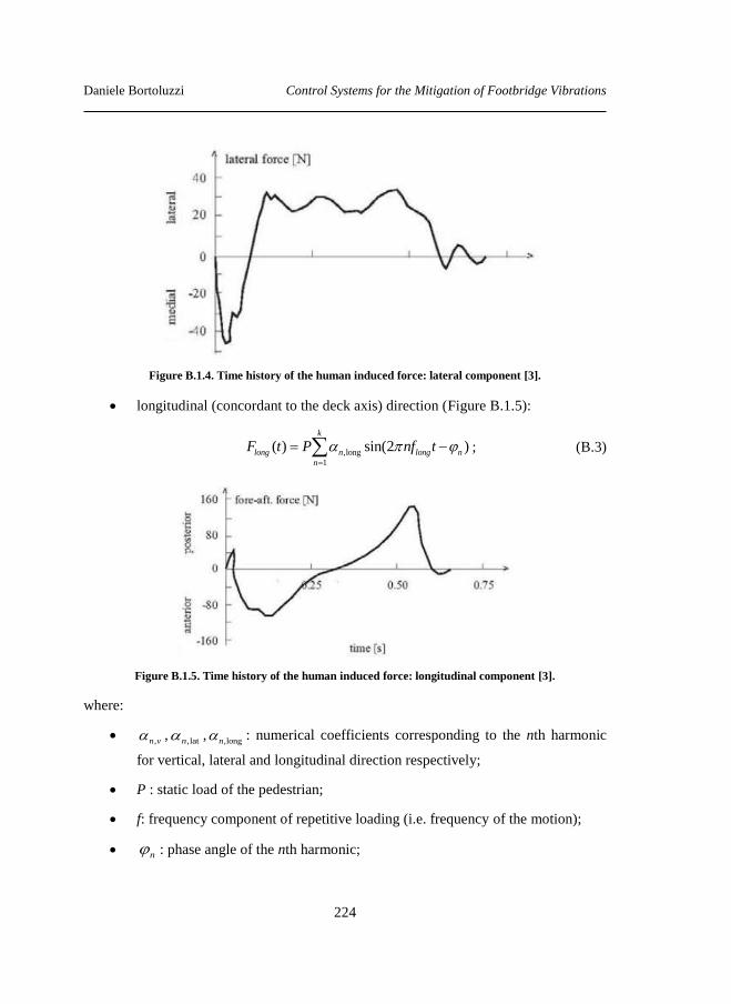
Daniele Bortoluzzi Control Systems for the Mitigation of Footbridge Vibrations
224
Figure B.1.4. Time history of the human induced force: lateral component [3].
longitudinal (concordant to the deck axis) direction (Figure B.1.5):
,long
1
( ) sin(2 )k
long n long n
n
F t P nf t
; (B.3)
Figure B.1.5. Time history of the human induced force: longitudinal component [3].
where:
,n v ,
,latn ,,longn : numerical coefficients corresponding to the nth harmonic
for vertical, lateral and longitudinal direction respectively;
P : static load of the pedestrian;
f: frequency component of repetitive loading (i.e. frequency of the motion);
n : phase angle of the nth harmonic;
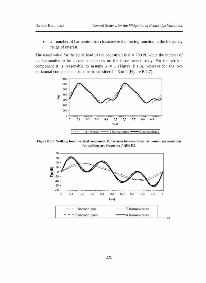
Daniele Bortoluzzi Control Systems for the Mitigation of Footbridge Vibrations
225
k : number of harmonics that characterize the forcing function in the frequency
range of interest.
The usual value for the static load of the pedestrian is P = 700 N, while the number of
the harmonics to be accounted depends on the forces under study. For the vertical
component it is reasonable to assume k = 1 (Figure B.1.6), whereas for the two
horizontal components it is better to consider k = 3 or 4 (Figure B.1.7).
Figure B.1.6. Walking force: vertical component. Differences between three harmonics representation
for walking step frequency f=2Hz [3].
a)
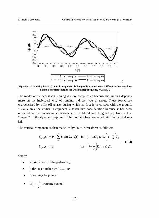
Daniele Bortoluzzi Control Systems for the Mitigation of Footbridge Vibrations
226
b)
Figure B.1.7. Walking force. a) lateral component; b) longitudinal component. Differences between four
harmonics representation for walking step frequency f=2Hz [3].
The model of the pedestrian running is more complicated because the running depends
more on the individual way of running and the type of shoes. These forces are
characterised by a lift-off phase, during which no foot is in contact with the ground.
Usually only the vertical component is taken into consideration because it has been
observed as the horizontal components, both lateral and longitudinal, have a low
“impact” on the dynamic response of the bridge when compared with the vertical one
[3].
The vertical component is then modelled by Fourier transform as follows:
; (B.4)
where:
P : static load of the pedestrian;
j: the step number, j=1,2,…, m;
fr: running frequency;
1
m
r
Tf
: running period.
,
1
,
1( ) sin(2 ) for 1
2
1( ) 0 for
2
k
r vert n r m m
n
r vert m m
F t P P nf t j T t j T
F t j T t jT
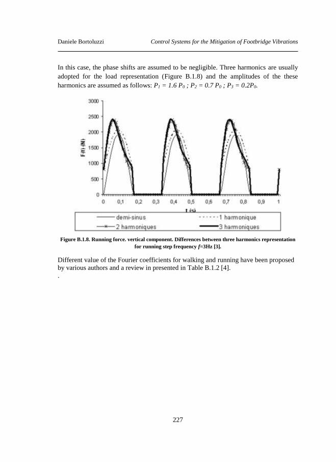
Daniele Bortoluzzi Control Systems for the Mitigation of Footbridge Vibrations
227
In this case, the phase shifts are assumed to be negligible. Three harmonics are usually
adopted for the load representation (Figure B.1.8) and the amplitudes of the these
harmonics are assumed as follows: P1 = 1.6 P0 ; P2 = 0.7 P0 ; P3 = 0.2P0.
Figure B.1.8. Running force. vertical component. Differences between three harmonics representation
for running step frequency f=3Hz [3].
Different value of the Fourier coefficients for walking and running have been proposed
by various authors and a review in presented in Table B.1.2 [4].
.
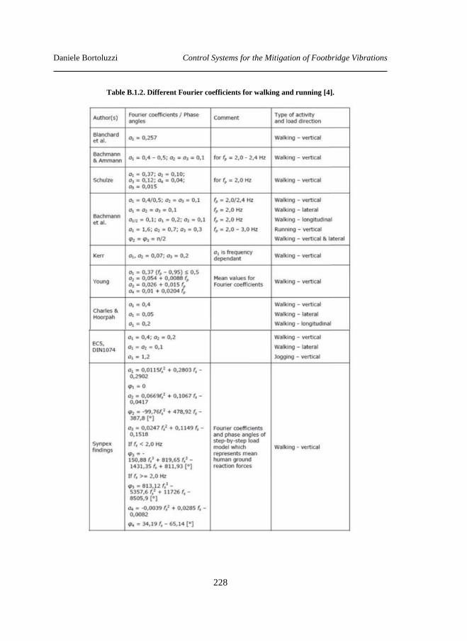
Daniele Bortoluzzi Control Systems for the Mitigation of Footbridge Vibrations
228
Table B.1.2. Different Fourier coefficients for walking and running [4].
Daniele Bortoluzzi Control Systems for the Mitigation of Footbridge Vibrations
229
B.2 References
[1] Guidelines for the design of footbridges. Fib bulletin 32, November 2005.
[2] Heinemeyer, C., Butz, C., Keil, A., Mark, S., Goldack, A., Trometer, S., Lukić,
M., Chabrolin, B., Lemaire, A., Martin, P., Cunha, Á., Caetano, E., 2009.
Design of Lightweight Footbridges for Human Induced Vibrations.
Background document in support to the implementation, harmonization and
further development of the Eurocodes, JRC European Commission,
Luxembourg.
[3] Footbridges: assessment of vibrational behaviour of footbridges under
pedestrian loading - Technical guide, 2006 – Sétra-AFGC.
[4] Živanović, S. et al., 2005. Vibration serviceability of footbridges under
humaninduced excitation: a literature review. Journal of Sound and Vibration
279, pp. 1-79.

Daniele Bortoluzzi Control Systems for the Mitigation of Footbridge Vibrations
230

Daniele Bortoluzzi Control Systems for the Mitigation of Footbridge Vibrations
231
Appendix C: Overview of some existing codes and
guidelines
In this chapter more details on the guidelines introduced in Chapter 2 about the comfort
evaluation of footbridges are given.
C.1 ISO 10137
ISO 10137 [1] provides a series of principles for the prediction of the vibrational
characteristics of a structure during the design stage. To assess the effects of the
vibrations, it is important to specify to the type of vibration source, its location and the
receiving element. The assessment of the response is evaluated by a numerical model.
The document gives the designer the choice of the comfort of level to be considered, but
states that pedestrian bridges must be so that the amplitude of the vibrations do not
cause discomfort to users. In the absence of more definitive data, the code suggests the
following maximum levels of vibration:
in the vertical direction (z-axis): the vibrations should not exceed those
obtained by a multiplicative factor of 60 in the selected reference system to
the relevant base curve represented in Figure C.1.1. When one or more
persons are at rest on the walkway the multiplicative factor of 30 should be
applied.
horizontal vibrations induced by pedestrian traffic or wind should not exceed
60 times the base curve for the horizontal direction (x and y- axis), see Figure
C.1.2.
For the calculation of root-mean-square values of the acceleration, an averaging time of
1 s is recommended. Furthermore the following scenarios have to be considered during
the calculation:
one person walking across the walkway and another (the receiver) standing at
mid-span;
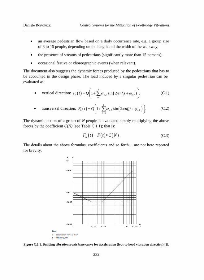
Daniele Bortoluzzi Control Systems for the Mitigation of Footbridge Vibrations
232
an average pedestrian flow based on a daily occurrence rate, e.g. a group size
of 8 to 15 people, depending on the length and the width of the walkway;
the presence of streams of pedestrians (significantly more than 15 persons);
occasional festive or choreographic events (when relevant).
The document also suggests the dynamic forces produced by the pedestrians that has to
be accounted in the design phase. The load induced by a singular pedestrian can be
evaluated as:
vertical direction: , ,
1
1 sin 2 ,k
v n v v n v
n
F t Q nf t
(C.1)
transversal direction: , ,
1
1 sin 2 .k
h n h h n h
n
F t Q nf t
(C.2)
The dynamic action of a group of N people is evaluated simply multiplying the above
forces by the coefficient C(N) (see Table C.1.1); that is:
NF t F t C N . (C.3)
The details about the above formulas, coefficients and so forth… are not here reported
for brevity.
Figure C.1.1. Building vibration z-axis base curve for acceleration (foot-to-head vibration direction) [1].
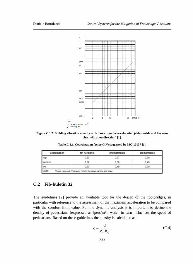
Daniele Bortoluzzi Control Systems for the Mitigation of Footbridge Vibrations
233
Figure C.1.2. Building vibration x- and y-axis base curve for acceleration (side-to-side and back-to-
chest vibration direction) [1].
Table C.1.1. Coordination factor C(N) suggested by ISO 10137 [1].
C.2 Fib-buletin 32
The guidelines [2] provide an available tool for the design of the footbridges, in
particular with reference to the assessment of the maximum acceleration to be compared
with the comfort limit value. For the dynamic analysis it is important to define the
density of pedestrians (expressed as [pers/m2], which in turn influences the speed of
pedestrians. Based on these guidelines the density is calculated as:
s eff
qv b
, (C.4)
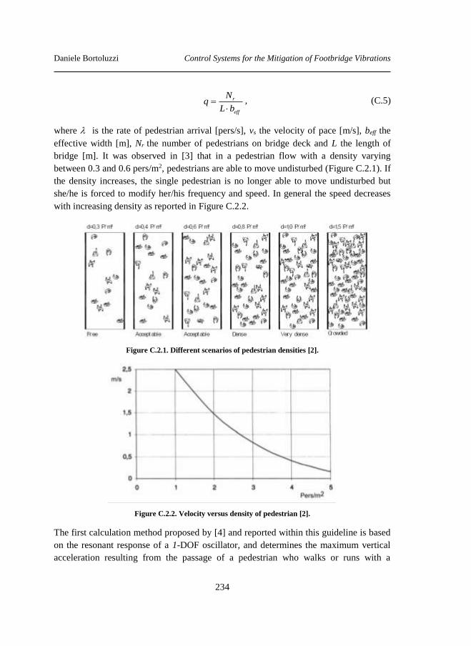
Daniele Bortoluzzi Control Systems for the Mitigation of Footbridge Vibrations
234
r
eff
Nq
L b
, (C.5)
where is the rate of pedestrian arrival [pers/s], vs the velocity of pace [m/s], beff the
effective width [m], Nr the number of pedestrians on bridge deck and L the length of
bridge [m]. It was observed in [3] that in a pedestrian flow with a density varying
between 0.3 and 0.6 pers/m2, pedestrians are able to move undisturbed (Figure C.2.1). If
the density increases, the single pedestrian is no longer able to move undisturbed but
she/he is forced to modify her/his frequency and speed. In general the speed decreases
with increasing density as reported in Figure C.2.2.
Figure C.2.1. Different scenarios of pedestrian densities [2].
Figure C.2.2. Velocity versus density of pedestrian [2].
The first calculation method proposed by [4] and reported within this guideline is based
on the resonant response of a 1-DOF oscillator, and determines the maximum vertical
acceleration resulting from the passage of a pedestrian who walks or runs with a
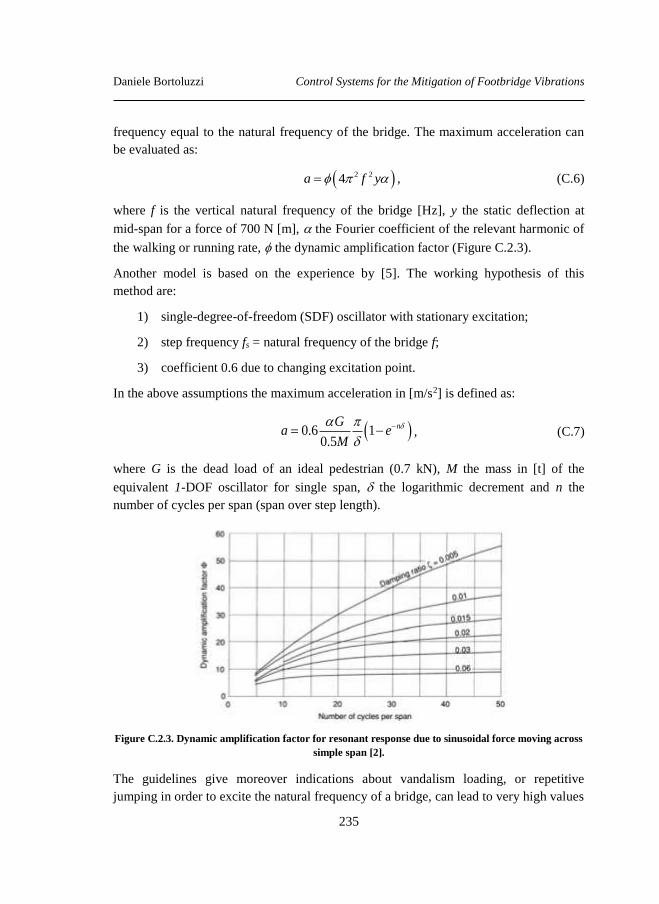
Daniele Bortoluzzi Control Systems for the Mitigation of Footbridge Vibrations
235
frequency equal to the natural frequency of the bridge. The maximum acceleration can
be evaluated as:
2 24a f y , (C.6)
where f is the vertical natural frequency of the bridge [Hz], y the static deflection at
mid-span for a force of 700 N [m], the Fourier coefficient of the relevant harmonic of
the walking or running rate, the dynamic amplification factor (Figure C.2.3).
Another model is based on the experience by [5]. The working hypothesis of this
method are:
1) single-degree-of-freedom (SDF) oscillator with stationary excitation;
2) step frequency fs = natural frequency of the bridge f;
3) coefficient 0.6 due to changing excitation point.
In the above assumptions the maximum acceleration in [m/s2] is defined as:
0.6 10.5
nGa e
M
, (C.7)
where G is the dead load of an ideal pedestrian (0.7 kN), M the mass in [t] of the
equivalent 1-DOF oscillator for single span, the logarithmic decrement and n the
number of cycles per span (span over step length).
Figure C.2.3. Dynamic amplification factor for resonant response due to sinusoidal force moving across
simple span [2].
The guidelines give moreover indications about vandalism loading, or repetitive
jumping in order to excite the natural frequency of a bridge, can lead to very high values
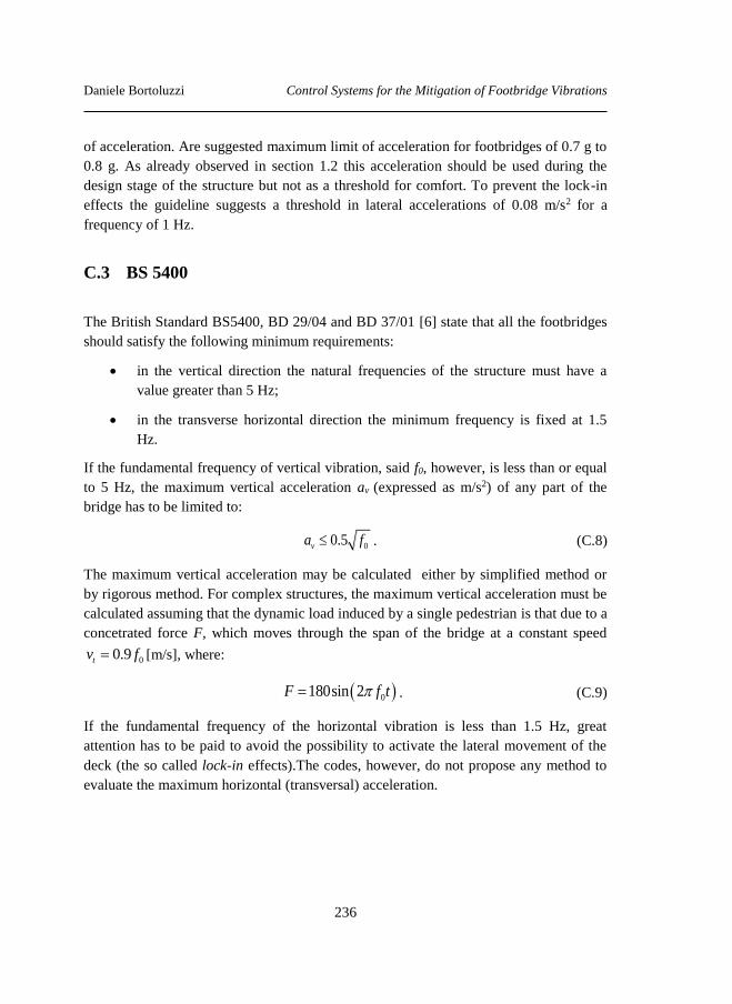
Daniele Bortoluzzi Control Systems for the Mitigation of Footbridge Vibrations
236
of acceleration. Are suggested maximum limit of acceleration for footbridges of 0.7 g to
0.8 g. As already observed in section 1.2 this acceleration should be used during the
design stage of the structure but not as a threshold for comfort. To prevent the lock-in
effects the guideline suggests a threshold in lateral accelerations of 0.08 m/s2 for a
frequency of 1 Hz.
C.3 BS 5400
The British Standard BS5400, BD 29/04 and BD 37/01 [6] state that all the footbridges
should satisfy the following minimum requirements:
in the vertical direction the natural frequencies of the structure must have a
value greater than 5 Hz;
in the transverse horizontal direction the minimum frequency is fixed at 1.5
Hz.
If the fundamental frequency of vertical vibration, said f0, however, is less than or equal
to 5 Hz, the maximum vertical acceleration av (expressed as m/s2) of any part of the
bridge has to be limited to:
00.5va f . (C.8)
The maximum vertical acceleration may be calculated either by simplified method or
by rigorous method. For complex structures, the maximum vertical acceleration must be
calculated assuming that the dynamic load induced by a single pedestrian is that due to a
concetrated force F, which moves through the span of the bridge at a constant speed
00.9tv f [m/s], where:
0180sin 2F f t . (C.9)
If the fundamental frequency of the horizontal vibration is less than 1.5 Hz, great
attention has to be paid to avoid the possibility to activate the lateral movement of the
deck (the so called lock-in effects).The codes, however, do not propose any method to
evaluate the maximum horizontal (transversal) acceleration.
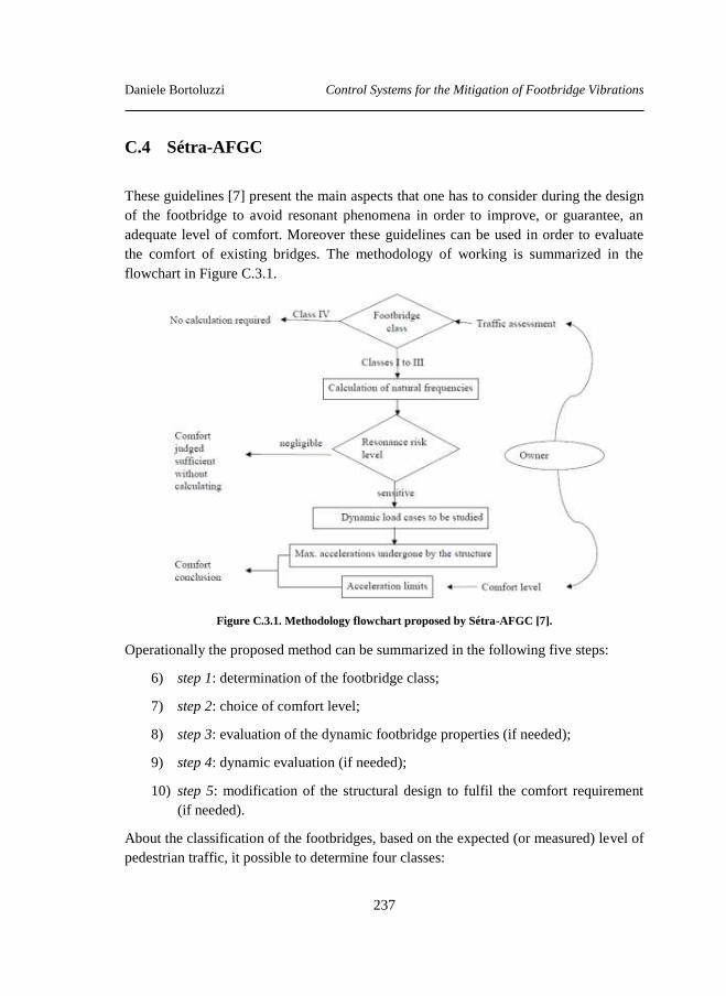
Daniele Bortoluzzi Control Systems for the Mitigation of Footbridge Vibrations
237
C.4 Sétra-AFGC
These guidelines [7] present the main aspects that one has to consider during the design
of the footbridge to avoid resonant phenomena in order to improve, or guarantee, an
adequate level of comfort. Moreover these guidelines can be used in order to evaluate
the comfort of existing bridges. The methodology of working is summarized in the
flowchart in Figure C.3.1.
Figure C.3.1. Methodology flowchart proposed by Sétra-AFGC [7].
Operationally the proposed method can be summarized in the following five steps:
6) step 1: determination of the footbridge class;
7) step 2: choice of comfort level;
8) step 3: evaluation of the dynamic footbridge properties (if needed);
9) step 4: dynamic evaluation (if needed);
10) step 5: modification of the structural design to fulfil the comfort requirement
(if needed).
About the classification of the footbridges, based on the expected (or measured) level of
pedestrian traffic, it possible to determine four classes:
Daniele Bortoluzzi Control Systems for the Mitigation of Footbridge Vibrations
238
Class IV: seldom used footbridge, built to link sparsely populated areas or to
ensure continuity of the pedestrian footpath across motorway or express lane
areas.
Class III: footbridge for standard use, that may occasionally be crossed by
large groups of people but that will never be loaded throughout its bearing
area.
Class II: urban footbridge linking up populated areas, subjected to heavy traffic
and that may occasionally be loaded throughout its bearing area.
Class I: urban footbridge linking up high pedestrian density areas (for instance,
nearby presence of a rail or underground station) or that is frequently used by
dense crowds (demonstrations, tourists, etc.), subjected to very heavy traffic.
The owner has to determine the footbridge class. It is always possible to select a higher
class to ensure/increase the comfort when needed. Class IV footbridges are considered
not to require any calculation to check the comfort performance. Anyway for very light
footbridges belonging to Class IV, at least Class III should be considered to ensure a
minimum level of comfort for the users.
The three levels of comfort can be defined as follows:
maximum comfort: accelerations are “imperceptible” to the users;
average comfort: accelerations are merely perceptible to the users;
minimum comfort: under seldom loading configurations, the accelerations
undergone are perceived by the users, but do not become intolerable.
The choice of the comfort level is normally influenced by the attitude of the persons22
using the footbridge and by its level of importance according to step 1. The level of
comfort is evaluated in reference to the acceleration undergone by the bridge using
different dynamic load cases. Due to the subjective nature of the comfort concept, the
guidelines present the comfortable limits in terms of four acceleration thresholds, see
Table C.3.1 and Table C.3.2, for vertical and horizontal accelerations respectively. The
first three ranges correspond to the maximum, mean and minimum comfort levels
described in the previous section; while the 4th range corresponds to an uncomfortable
situation.
22 In this choice the designer should be more demanding on behalf of particularly sensitive users
as schoolchildren, disabled people and so forth…, and more tolerant in case of all those
footbridges rarely used by pedestrians.
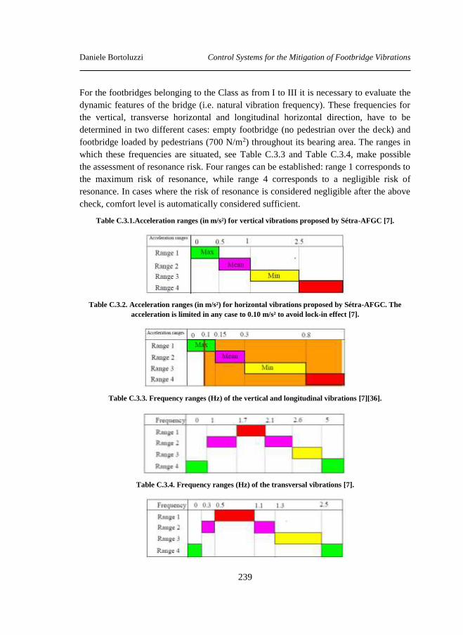
Daniele Bortoluzzi Control Systems for the Mitigation of Footbridge Vibrations
239
For the footbridges belonging to the Class as from I to III it is necessary to evaluate the
dynamic features of the bridge (i.e. natural vibration frequency). These frequencies for
the vertical, transverse horizontal and longitudinal horizontal direction, have to be
determined in two different cases: empty footbridge (no pedestrian over the deck) and
footbridge loaded by pedestrians (700 N/m2) throughout its bearing area. The ranges in
which these frequencies are situated, see Table C.3.3 and Table C.3.4, make possible
the assessment of resonance risk. Four ranges can be established: range 1 corresponds to
the maximum risk of resonance, while range 4 corresponds to a negligible risk of
resonance. In cases where the risk of resonance is considered negligible after the above
check, comfort level is automatically considered sufficient.
Table C.3.1.Acceleration ranges (in m/s²) for vertical vibrations proposed by Sétra-AFGC [7].
Table C.3.2. Acceleration ranges (in m/s²) for horizontal vibrations proposed by Sétra-AFGC. The
acceleration is limited in any case to 0.10 m/s² to avoid lock-in effect [7].
Table C.3.3. Frequency ranges (Hz) of the vertical and longitudinal vibrations [7][36].
Table C.3.4. Frequency ranges (Hz) of the transversal vibrations [7].

Daniele Bortoluzzi Control Systems for the Mitigation of Footbridge Vibrations
240
If the above evaluation shows the possibility of resonance risk a more detailed analysis
must to be carried out (step 4). In this case three different cases of dynamic loads have
to be considered:
Case 1: sparse and dense crowds.
This case regards the study of the pedestrian bridges belonging to Class II and III. The
number of pedestrians involved, within the hypothesis crowd uniformly distributed over
the deck, is equal to:
N S d , (C.10)
in which S indicates the deck area, and d pedestrian density. For Class III footbridges
the density d of pedestrian must be taken equal to 0.5 pedestrians/m2; while d = 0.8
pedestrians/m2 for Class II footbridges. The equivalent number of pedestrians Neq (all in
phase and at the same frequency) able to produce the same effects on structure as
random pedestrian is:
10.8eqN N , (C.11)
where is the critical damping ratio (Table C.3.5).
Table C.3.5. Typical critical damping ratio [7].
Table C.3.6. Case 1 - Loads per unit of area proposed by Sétra-AFGC. Below: factor ψ for vertical and
longitudinal vibrations on the left, and for lateral vibrations on the right [7].
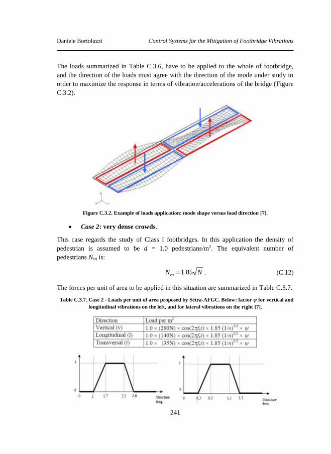
Daniele Bortoluzzi Control Systems for the Mitigation of Footbridge Vibrations
241
The loads summarized in Table C.3.6, have to be applied to the whole of footbridge,
and the direction of the loads must agree with the direction of the mode under study in
order to maximize the response in terms of vibration/accelerations of the bridge (Figure
C.3.2).
Figure C.3.2. Example of loads application: mode shape versus load direction [7].
Case 2: very dense crowds.
This case regards the study of Class I footbridges. In this application the density of
pedestrian is assumed to be d = 1.0 pedestrians/m2. The equivalent number of
pedestrians Neq is:
1.85eqN N . (C.12)
The forces per unit of area to be applied in this situation are summarized in Table C.3.7.
Table C.3.7. Case 2 - Loads per unit of area proposed by Sétra-AFGC. Below: factor ψ for vertical and
longitudinal vibrations on the left, and for lateral vibrations on the right [7].
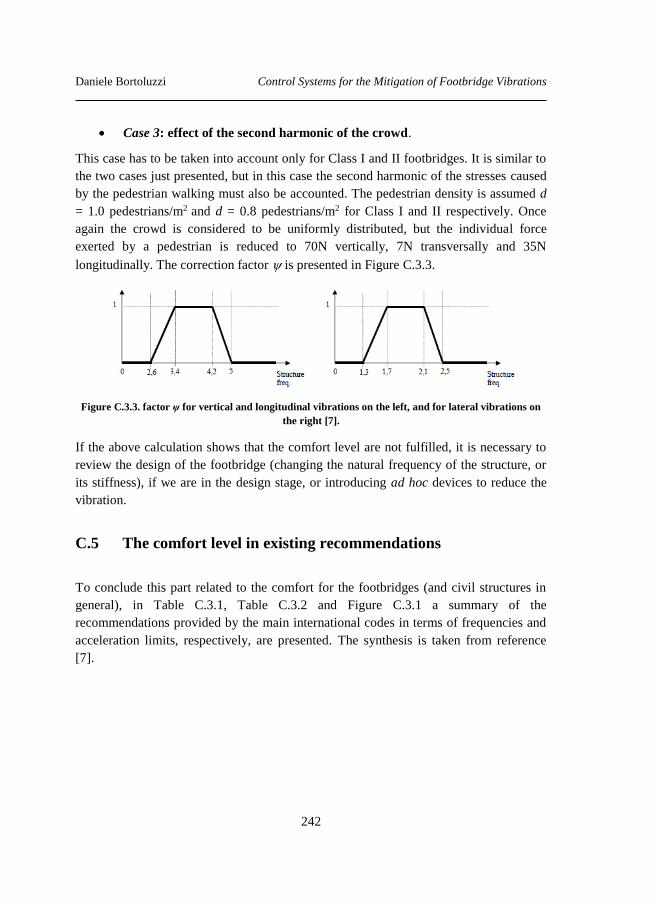
Daniele Bortoluzzi Control Systems for the Mitigation of Footbridge Vibrations
242
Case 3: effect of the second harmonic of the crowd.
This case has to be taken into account only for Class I and II footbridges. It is similar to
the two cases just presented, but in this case the second harmonic of the stresses caused
by the pedestrian walking must also be accounted. The pedestrian density is assumed d
= 1.0 pedestrians/m2 and d = 0.8 pedestrians/m2 for Class I and II respectively. Once
again the crowd is considered to be uniformly distributed, but the individual force
exerted by a pedestrian is reduced to 70N vertically, 7N transversally and 35N
longitudinally. The correction factor is presented in Figure C.3.3.
Figure C.3.3. factor ψ for vertical and longitudinal vibrations on the left, and for lateral vibrations on
the right [7].
If the above calculation shows that the comfort level are not fulfilled, it is necessary to
review the design of the footbridge (changing the natural frequency of the structure, or
its stiffness), if we are in the design stage, or introducing ad hoc devices to reduce the
vibration.
C.5 The comfort level in existing recommendations
To conclude this part related to the comfort for the footbridges (and civil structures in
general), in Table C.3.1, Table C.3.2 and Figure C.3.1 a summary of the
recommendations provided by the main international codes in terms of frequencies and
acceleration limits, respectively, are presented. The synthesis is taken from reference
[7].
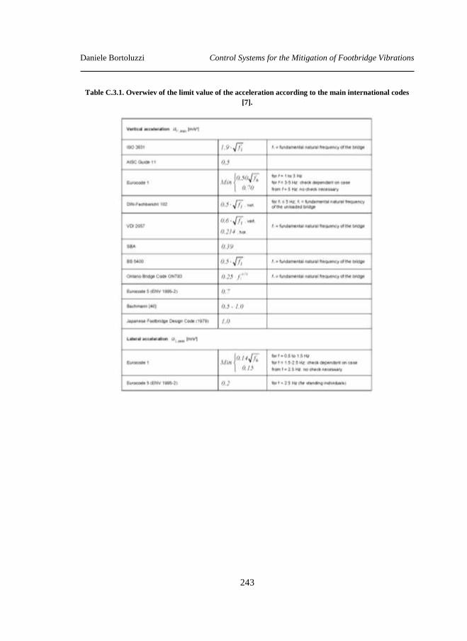
Daniele Bortoluzzi Control Systems for the Mitigation of Footbridge Vibrations
243
Table C.3.1. Overwiev of the limit value of the acceleration according to the main international codes
[7].
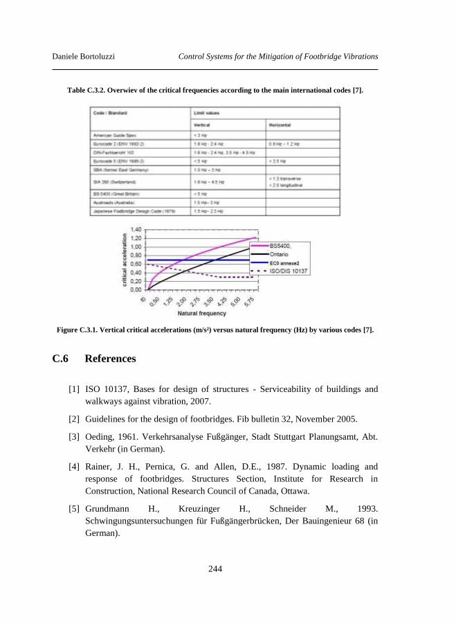
Daniele Bortoluzzi Control Systems for the Mitigation of Footbridge Vibrations
244
Table C.3.2. Overwiev of the critical frequencies according to the main international codes [7].
Figure C.3.1. Vertical critical accelerations (m/s²) versus natural frequency (Hz) by various codes [7].
C.6 References
[1] ISO 10137, Bases for design of structures - Serviceability of buildings and
walkways against vibration, 2007.
[2] Guidelines for the design of footbridges. Fib bulletin 32, November 2005.
[3] Oeding, 1961. Verkehrsanalyse Fußgänger, Stadt Stuttgart Planungsamt, Abt.
Verkehr (in German).
[4] Rainer, J. H., Pernica, G. and Allen, D.E., 1987. Dynamic loading and
response of footbridges. Structures Section, Institute for Research in
Construction, National Research Council of Canada, Ottawa.
[5] Grundmann H., Kreuzinger H., Schneider M., 1993.
Schwingungsuntersuchungen für Fußgängerbrücken, Der Bauingenieur 68 (in
German).

Daniele Bortoluzzi Control Systems for the Mitigation of Footbridge Vibrations
245
[6] BS5400, Part 2, Appendix C, Vibration Serviceability Requirements for Foot
and Cycle Track Bridges. British Standards Institution, 1978.
[7] Footbridges: assessment of vibrational behaviour of footbridges under
pedestrian loading - Technical guide, 2006 – Sétra-AFGC.

Daniele Bortoluzzi Control Systems for the Mitigation of Footbridge Vibrations
246
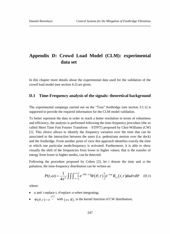
Daniele Bortoluzzi Control Systems for the Mitigation of Footbridge Vibrations
247
Appendix D: Crowd Load Model (CLM): experimental
data set
In this chapter more details about the experimental data used for the validation of the
crowd load model (see section 4.2) are given.
D.1 Time-Frequency analysis of the signals: theoretical background
The experimental campaign carried out on the “Tesa” footbridge (see section 3.1.1) is
supported to provide the required information for the CLM model validation.
To better represent the data in order to reach a better resolution in terms of robustness
and efficiency, the analysis is performed following the time-frequency procedure (the so
called Short Time Fast Fourier Transform – STFFT) proposed by Choi-Williams (CW)
[1]. This choice allows to identify the frequency variation over the time that can be
associated to the interaction between the users (i.e. pedestrians motion over the deck)
and the footbridge. From another point of view this approach identifies exactly the time
at which one particular mode/frequency is activated. Furthermore, it is able to show
visually the shift of the frequencies from lower to higher values; that is the transfer of
energy from lower to higher modes, can be detected.
Following the procedure proposed by Cohen [2], let t denote the time and the
pulsation, the time-frequency distribution can be written as:
,12
1( , ) , ,
4
i t u i
tP t e e R t dud d
(D.1)
where:
u and replace t, replace when integrating;
2 2
, se
with s R , is the kernel function of CW distribution;
Daniele Bortoluzzi Control Systems for the Mitigation of Footbridge Vibrations
248
,1 , / 2 / 2tR t x u x u is the autocorrelation function in which x(t) is the
input signal, t the time and / 2u t .
Introducing now the Fourier transform W(t-u) for the above kernel function in equation
(D.1):
,12
1( , ) ,
4
i
tP t W t u e R t dud
; (D.2)
As an example the time-frequency analysis is performed for the test carried out on
“Tesa2 footbridge, and labelled as test B3 (see section 3.1.1). The main results for the
data acquired by sensor WSa2 (see Figure 3.1.3) along the transversal (Y) and gravity
(Z) axis are summarized in Figure D.1.1 and Figure D.1.2 respectively.
During this test, only one frequency clearly appears at 1.35 Hz, and it is constant over
the entire duration of the data acquisition. Another frequency appears at 5.00 Hz in the
time period between 50 and 70 sec for the right-to-left crossing, and in the time period
from 100 to 160 sec for the left-to-right crossing. This plot shows many vertical lines; in
particular, one can observe that in the time period between 125 and 140 sec, there is a
consistent frequency shift, due to the overlapping of the waves associated to the
movement of the pedestrians from the sides toward the mid-span. Also along the Z axis
only one frequency clearly appears at 2.00 Hz, and it is activated in the time period
between 50 and 80 sec for the right-to-left crossing, and between 100 and 160 sec for
the left-to-right crossing. Moreover one more frequency of 6.00 Hz seems to be
“slightly” activated between 50 and 70 sec for the right-to-left crossing, and between
130 and 150 sec for the left-to-right crossing.
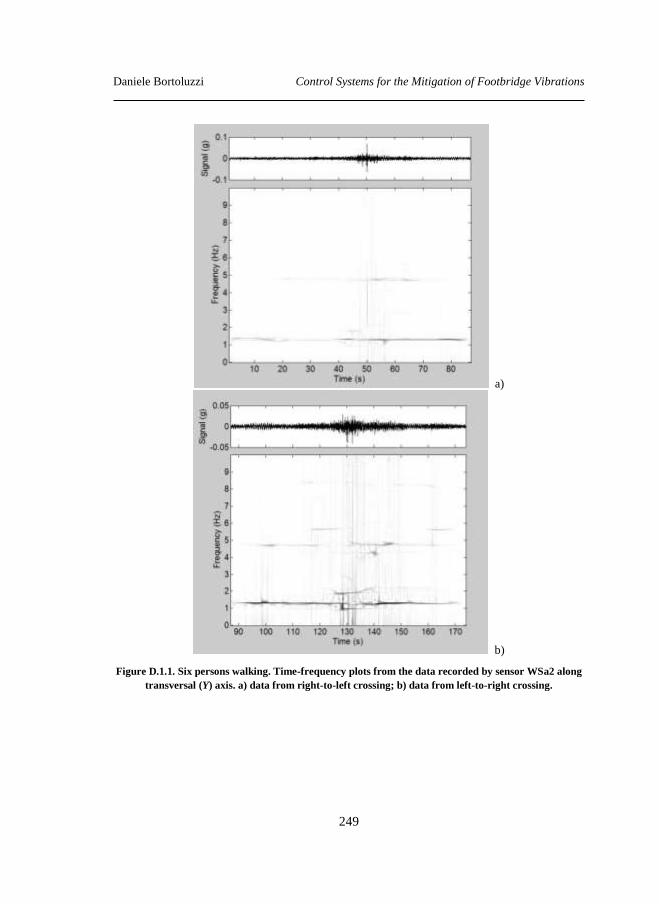
Daniele Bortoluzzi Control Systems for the Mitigation of Footbridge Vibrations
249
a)
b)
Figure D.1.1. Six persons walking. Time-frequency plots from the data recorded by sensor WSa2 along
transversal (Y) axis. a) data from right-to-left crossing; b) data from left-to-right crossing.
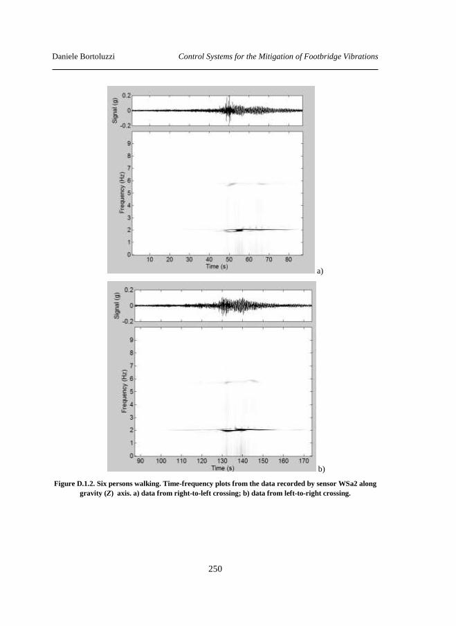
Daniele Bortoluzzi Control Systems for the Mitigation of Footbridge Vibrations
250
a)
b)
Figure D.1.2. Six persons walking. Time-frequency plots from the data recorded by sensor WSa2 along
gravity (Z) axis. a) data from right-to-left crossing; b) data from left-to-right crossing.
Daniele Bortoluzzi Control Systems for the Mitigation of Footbridge Vibrations
251
D.2 Experimental data analysis
To validate the proposed CLM model, in necessary to identify a set of experimental data
that will be compared with the numerical simulation. By the way, in this section, the
data acquired during the tests B presented in section 3.1.1 are analyzed and discussed.
To give an easier interpretation of these data, each record is classified into two different
sets: crossing from the right to the left side of the footbridge (labelled as RtoL), and
from the left to the ride side (labelled as RtoL) ([3] and [4]).
To have a clear idea about the acquired data, the numerical analysis of the data are
performed following the time-frequency technique (STFFT) presented in the previous
section.
Here below the results achieved by the analysis are discussed.
- test B1
This test consists of collecting records of the accelerations of the footbridge due to a
round trip along the deck. The mass of the person is 85 Kg. Further details about this
test are summarized in Table D.2.1. The results achieved for the measurements taken by
sensor WSa2 along the transversal Y and vertical (gravity) Z axes are plotted in Figure
D.2.1 and Figure D.2.2 respectively.
Table D.2.1. Walking (round trip) of one person.
Type ID
Day/Time November 7,2013 / 2.48 pm
Test type walking (round trip)
Air temperature 15°C
Pedestrian(s) num. 1 person
Total Pedestrian(s) mass 85 Kg
Total time duration ≈2:30 min
RtoL time duration ≈1:15 min
LtoR time duration ≈1:15 min
Average velocity of the pedestrian(s) 1.45 m/s

Daniele Bortoluzzi Control Systems for the Mitigation of Footbridge Vibrations
252
a)
b)
Figure D.2.1. Time-frequency plot from the data taken by sensorWSa2 along Y transversal axis during
test Ia. a) RtoL data ; b) LoR data
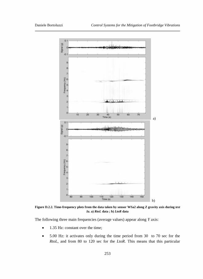
Daniele Bortoluzzi Control Systems for the Mitigation of Footbridge Vibrations
253
a)
b)
Figure D.2.2. Time-frequency plots from the data taken by sensor WSa2 along Z gravity axis during test
Ia. a) RtoL data ; b) LtoR data
The following three main frequencies (average values) appear along Y axis:
1.35 Hz: constant over the time;
5.00 Hz: it activates only during the time period from 30 to 70 sec for the
RtoL, and from 80 to 120 sec for the LtoR. This means that this particular
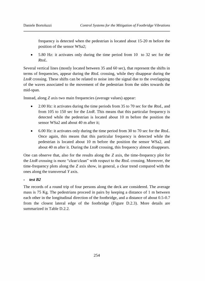
Daniele Bortoluzzi Control Systems for the Mitigation of Footbridge Vibrations
254
frequency is detected when the pedestrian is located about 15-20 m before the
position of the sensor WSa2;
5.80 Hz: it activates only during the time period from 10 to 32 sec for the
RtoL.
Several vertical lines (mostly located between 35 and 60 sec), that represent the shifts in
terms of frequencies, appear during the RtoL crossing, while they disappear during the
LtoR crossing. These shifts can be related to noise into the signal due to the overlapping
of the waves associated to the movement of the pedestrian from the sides towards the
mid-span.
Instead, along Z axis two main frequencies (average values) appear:
2.00 Hz: it activates during the time periods from 35 to 70 sec for the RtoL, and
from 105 to 150 sec for the LtoR. This means that this particular frequency is
detected while the pedestrian is located about 10 m before the position the
sensor WSa2 and about 40 m after it;
6.00 Hz: it activates only during the time period from 30 to 70 sec for the RtoL.
Once again, this means that this particular frequency is detected while the
pedestrian is located about 10 m before the position the sensor WSa2, and
about 40 m after it. During the LtoR crossing, this frequency almost disappears.
One can observe that, also for the results along the Z axis, the time-frequency plot for
the LtoR crossing is more “clear/clean” with respect to the RtoL crossing. Moreover, the
time-frequency plots along the Z axis show, in general, a clear trend compared with the
ones along the transversal Y axis.
- test B2
The records of a round trip of four persons along the deck are considered. The average
mass is 75 Kg. The pedestrians proceed in pairs by keeping a distance of 1 m between
each other in the longitudinal direction of the footbridge, and a distance of about 0.5-0.7
from the closest lateral edge of the footbridge (Figure D.2.3). More details are
summarized in Table D.2.2.
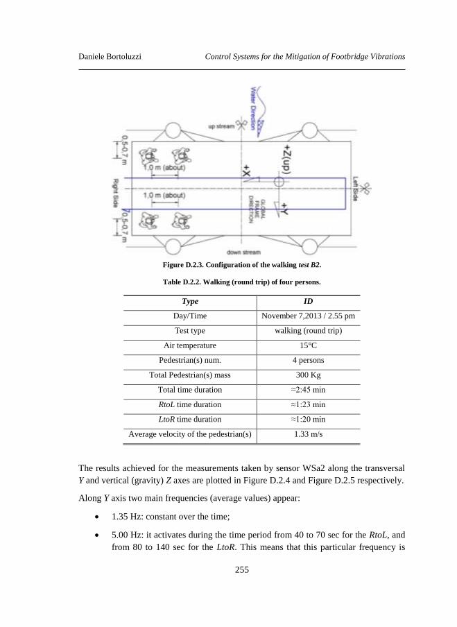
Daniele Bortoluzzi Control Systems for the Mitigation of Footbridge Vibrations
255
Figure D.2.3. Configuration of the walking test B2.
Table D.2.2. Walking (round trip) of four persons.
Type ID
Day/Time November 7,2013 / 2.55 pm
Test type walking (round trip)
Air temperature 15°C
Pedestrian(s) num. 4 persons
Total Pedestrian(s) mass 300 Kg
Total time duration ≈2:45 min
RtoL time duration ≈1:23 min
LtoR time duration ≈1:20 min
Average velocity of the pedestrian(s) 1.33 m/s
The results achieved for the measurements taken by sensor WSa2 along the transversal
Y and vertical (gravity) Z axes are plotted in Figure D.2.4 and Figure D.2.5 respectively.
Along Y axis two main frequencies (average values) appear:
1.35 Hz: constant over the time;
5.00 Hz: it activates during the time period from 40 to 70 sec for the RtoL, and
from 80 to 140 sec for the LtoR. This means that this particular frequency is

Daniele Bortoluzzi Control Systems for the Mitigation of Footbridge Vibrations
256
detected when the pedestrian is located about 15-20 m before the position of
the sensor WSa2.
One can observe, moreover, that several vertical lines (mostly located between 46 and
60 sec and between 120 and130 sec), which represent the frequency shifts, appear
during both the RtoL and the LtoR crossings. Furthermore one more frequency of about
2.00 Hz appears at about 130 sec up to the end of the record. All these facts can be
related, as previously observed, to the overlapping of the waves associated to the
movement of the pedestrians from the sides towards the mid-span of the bridge.
Along Z axis the results appear are more “clear/clean”, and in particular only two main
frequencies (average values) are highlighted:
2.00 Hz: it activates during the time period from 35 to 70 sec for the RtoL; and
from 110 to 160 sec for the LtoR. This mean that this particular frequency is
detected while the pedestrian is located about 10 m before the position of
sensor WSa2, and about 40 m after it;
6.00 Hz: it activates during the time period from 30 to 70 sec for the RtoL only.
This means that this particular frequency is detected while the pedestrian is
located about 10 m before the position of sensor WSa2, and about 40 m after it.
During the LtoR crossing this frequency almost disappears.
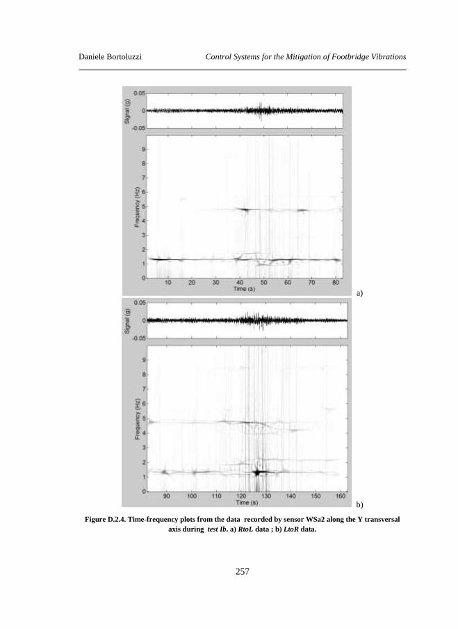
Daniele Bortoluzzi Control Systems for the Mitigation of Footbridge Vibrations
257
a)
b)
Figure D.2.4. Time-frequency plots from the data recorded by sensor WSa2 along the Y transversal
axis during test Ib. a) RtoL data ; b) LtoR data.
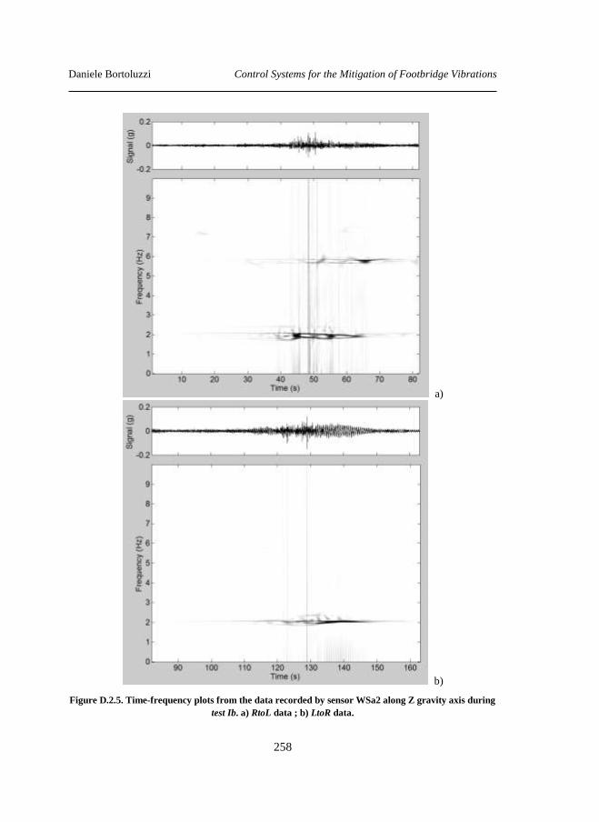
Daniele Bortoluzzi Control Systems for the Mitigation of Footbridge Vibrations
258
a)
b)
Figure D.2.5. Time-frequency plots from the data recorded by sensor WSa2 along Z gravity axis during
test Ib. a) RtoL data ; b) LtoR data.
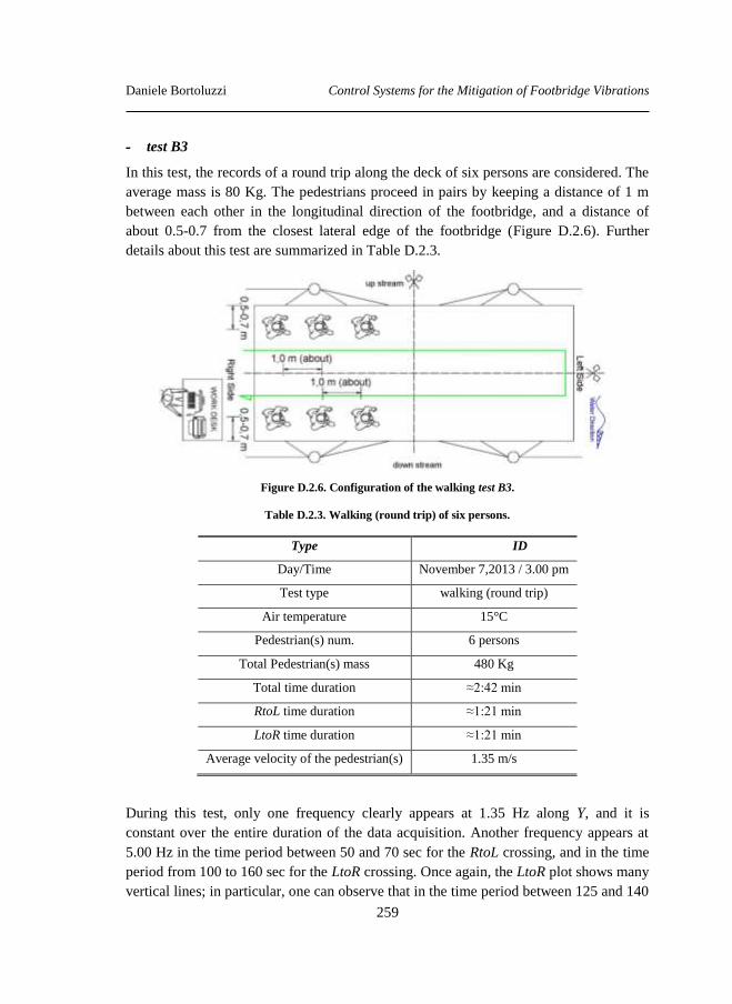
Daniele Bortoluzzi Control Systems for the Mitigation of Footbridge Vibrations
259
- test B3
In this test, the records of a round trip along the deck of six persons are considered. The
average mass is 80 Kg. The pedestrians proceed in pairs by keeping a distance of 1 m
between each other in the longitudinal direction of the footbridge, and a distance of
about 0.5-0.7 from the closest lateral edge of the footbridge (Figure D.2.6). Further
details about this test are summarized in Table D.2.3.
Figure D.2.6. Configuration of the walking test B3.
Table D.2.3. Walking (round trip) of six persons.
Type ID
Day/Time November 7,2013 / 3.00 pm
Test type walking (round trip)
Air temperature 15°C
Pedestrian(s) num. 6 persons
Total Pedestrian(s) mass 480 Kg
Total time duration ≈2:42 min
RtoL time duration ≈1:21 min
LtoR time duration ≈1:21 min
Average velocity of the pedestrian(s) 1.35 m/s
During this test, only one frequency clearly appears at 1.35 Hz along Y, and it is
constant over the entire duration of the data acquisition. Another frequency appears at
5.00 Hz in the time period between 50 and 70 sec for the RtoL crossing, and in the time
period from 100 to 160 sec for the LtoR crossing. Once again, the LtoR plot shows many
vertical lines; in particular, one can observe that in the time period between 125 and 140

Daniele Bortoluzzi Control Systems for the Mitigation of Footbridge Vibrations
260
sec, there is a consistent frequency shift, due to the overlapping of the waves associated
to the movement of the pedestrians from the sides toward the mid-span (Figure D.2.7).
Also along the Z axis only one frequency clearly appears at 2.00 Hz, and it is activated
in the time period between 50 and 80 sec for the RtoL crossing, and between 100 and
160 sec for the LtoR crossing. Moreover one more frequency of 6.00 Hz seems to be
“slightly” activated between 50 and 70 sec for the RtoL crossing, and between 130 and
150 sec for the LtoR crossing (Figure D.2.8).
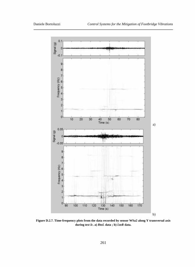
Daniele Bortoluzzi Control Systems for the Mitigation of Footbridge Vibrations
261
a)
b)
Figure D.2.7. Time-frequency plots from the data recorded by sensor WSa2 along Y transversal axis
during test Ic. a) RtoL data ; b) LtoR data.
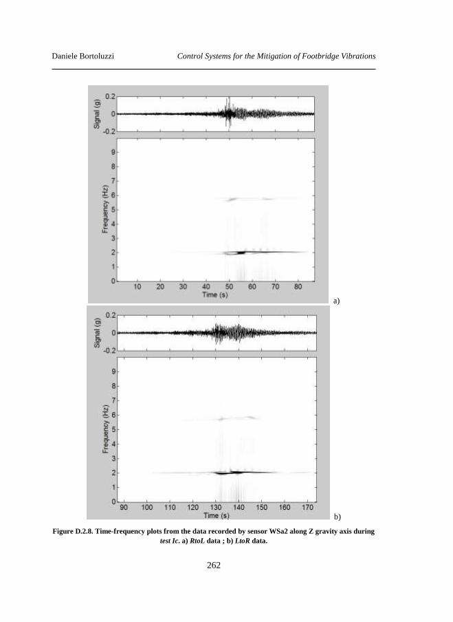
Daniele Bortoluzzi Control Systems for the Mitigation of Footbridge Vibrations
262
a)
b)
Figure D.2.8. Time-frequency plots from the data recorded by sensor WSa2 along Z gravity axis during
test Ic. a) RtoL data ; b) LtoR data.
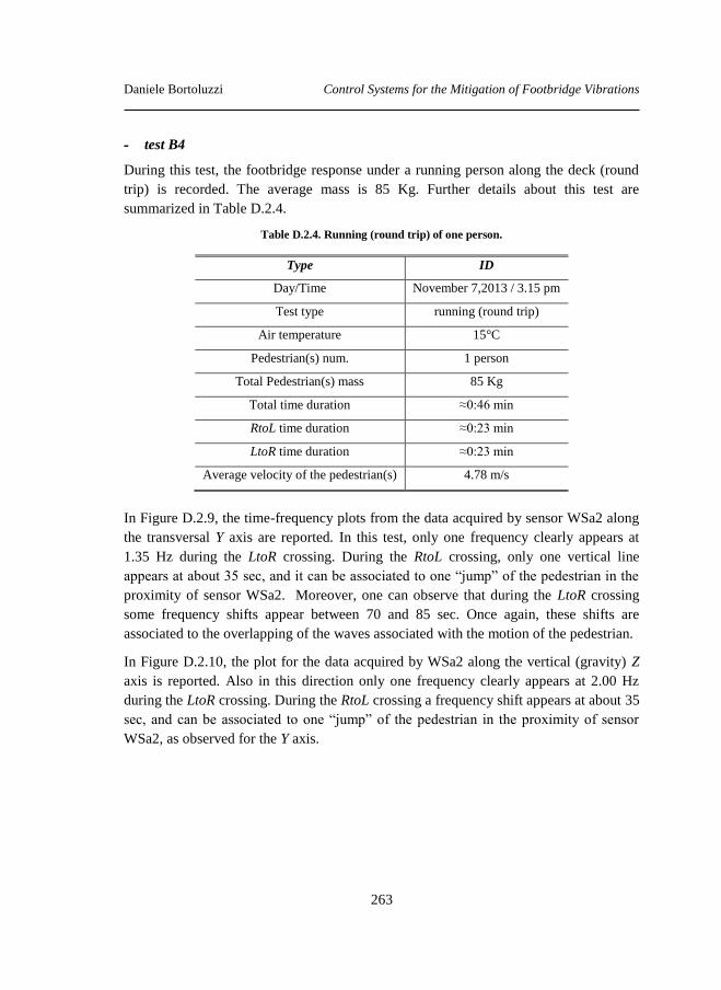
Daniele Bortoluzzi Control Systems for the Mitigation of Footbridge Vibrations
263
- test B4
During this test, the footbridge response under a running person along the deck (round
trip) is recorded. The average mass is 85 Kg. Further details about this test are
summarized in Table D.2.4.
Table D.2.4. Running (round trip) of one person.
Type ID
Day/Time November 7,2013 / 3.15 pm
Test type running (round trip)
Air temperature 15°C
Pedestrian(s) num. 1 person
Total Pedestrian(s) mass 85 Kg
Total time duration ≈0:46 min
RtoL time duration ≈0:23 min
LtoR time duration ≈0:23 min
Average velocity of the pedestrian(s) 4.78 m/s
In Figure D.2.9, the time-frequency plots from the data acquired by sensor WSa2 along
the transversal Y axis are reported. In this test, only one frequency clearly appears at
1.35 Hz during the LtoR crossing. During the RtoL crossing, only one vertical line
appears at about 35 sec, and it can be associated to one “jump” of the pedestrian in the
proximity of sensor WSa2. Moreover, one can observe that during the LtoR crossing
some frequency shifts appear between 70 and 85 sec. Once again, these shifts are
associated to the overlapping of the waves associated with the motion of the pedestrian.
In Figure D.2.10, the plot for the data acquired by WSa2 along the vertical (gravity) Z
axis is reported. Also in this direction only one frequency clearly appears at 2.00 Hz
during the LtoR crossing. During the RtoL crossing a frequency shift appears at about 35
sec, and can be associated to one “jump” of the pedestrian in the proximity of sensor
WSa2, as observed for the Y axis.
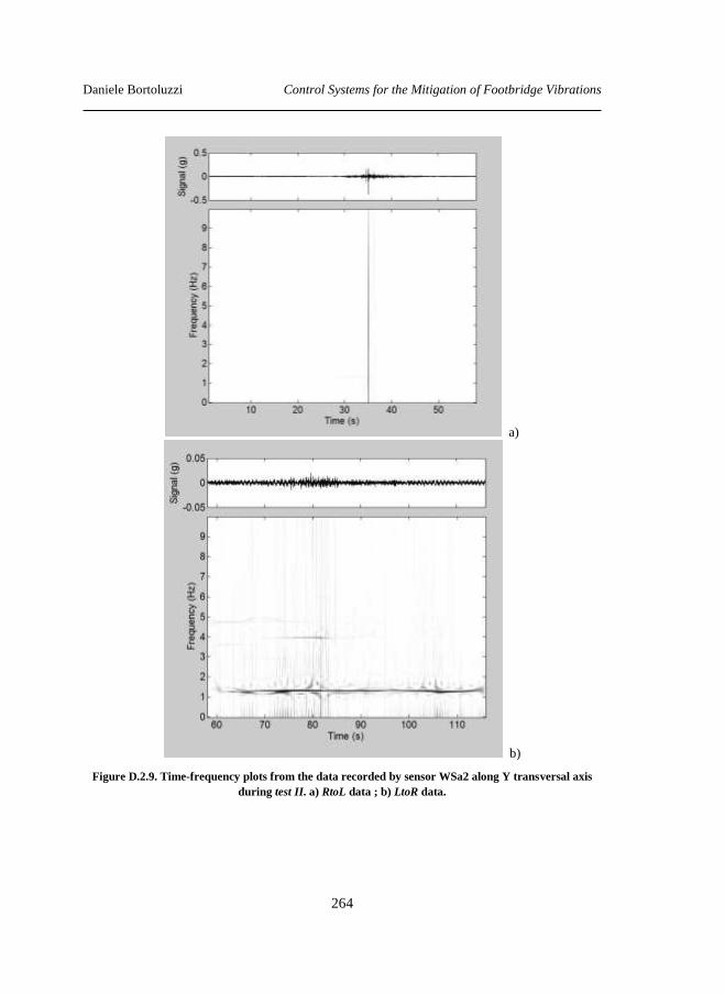
Daniele Bortoluzzi Control Systems for the Mitigation of Footbridge Vibrations
264
a)
b)
Figure D.2.9. Time-frequency plots from the data recorded by sensor WSa2 along Y transversal axis
during test II. a) RtoL data ; b) LtoR data.
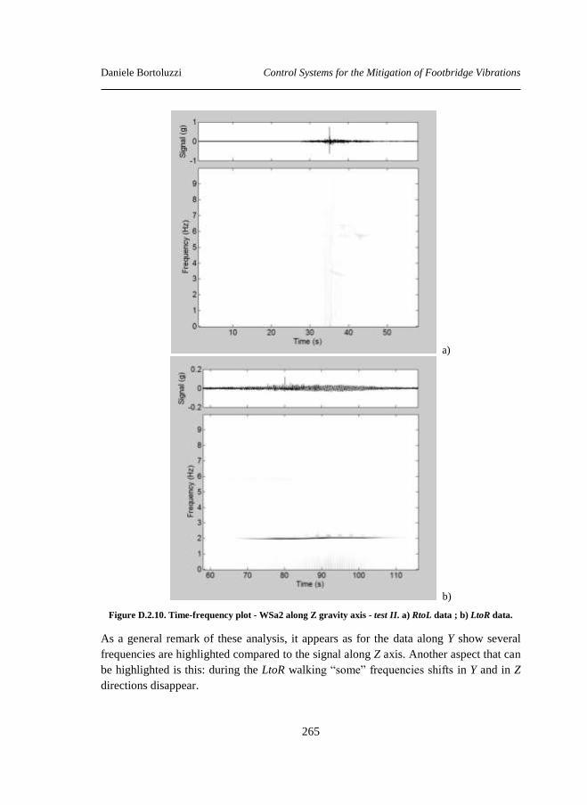
Daniele Bortoluzzi Control Systems for the Mitigation of Footbridge Vibrations
265
a)
b)
Figure D.2.10. Time-frequency plot - WSa2 along Z gravity axis - test II. a) RtoL data ; b) LtoR data.
As a general remark of these analysis, it appears as for the data along Y show several
frequencies are highlighted compared to the signal along Z axis. Another aspect that can
be highlighted is this: during the LtoR walking “some” frequencies shifts in Y and in Z
directions disappear.
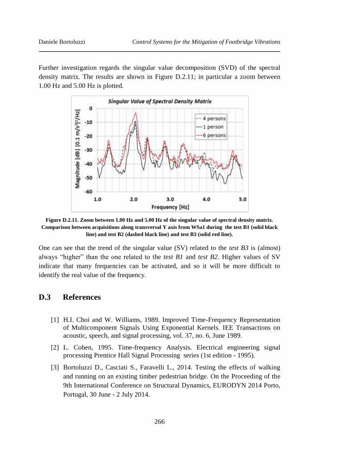
Daniele Bortoluzzi Control Systems for the Mitigation of Footbridge Vibrations
266
Further investigation regards the singular value decomposition (SVD) of the spectral
density matrix. The results are shown in Figure D.2.11; in particular a zoom between
1.00 Hz and 5.00 Hz is plotted.
Figure D.2.11. Zoom between 1.00 Hz and 5.00 Hz of the singular value of spectral density matrix.
Comparison between acquisitions along transversal Y axis from WSa1 during the test B1 (solid black
line) and test B2 (dashed black line) and test B3 (solid red line).
One can see that the trend of the singular value (SV) related to the test B3 is (almost)
always “higher” than the one related to the test B1 and test B2. Higher values of SV
indicate that many frequencies can be activated, and so it will be more difficult to
identify the real value of the frequency.
D.3 References
[1] H.I. Choi and W. Williams, 1989. Improved Time-Frequency Representation
of Multicomponent Signals Using Exponential Kernels. IEE Transactions on
acoustic, speech, and signal processing, vol. 37, no. 6, June 1989.
[2] L. Cohen, 1995. Time-frequency Analysis. Electrical engineering signal
processing Prentice Hall Signal Processing series (1st edition - 1995).
[3] Bortoluzzi D., Casciati S., Faravelli L., 2014. Testing the effects of walking
and running on an existing timber pedestrian bridge. On the Proceeding of the
9th International Conference on Structural Dynamics, EURODYN 2014 Porto,
Portugal, 30 June - 2 July 2014.

Daniele Bortoluzzi Control Systems for the Mitigation of Footbridge Vibrations
267
[4] S. Casciati, F. Casciati, L. Faravelli and D. Bortoluzzi, 2014. Modelling The
Human Induced Vibrations In A Cable-Stayed Pedestrian Timber Bridge. On
the Proceeding of the 7th European Workshop on Structural Health Monitoring
– EWSHM2014, July 8-11, 2014. La Cité, Nantes, France.

Daniele Bortoluzzi Control Systems for the Mitigation of Footbridge Vibrations
268
Daniele Bortoluzzi Control Systems for the Mitigation of Footbridge Vibrations
269
Acknowledgements
Mi sembra doveroso, arrivato a questo punto, fare alcuni ringraziamenti. Innanzitutto vorrei
ringraziare la Prof.ssa Faravelli Lucia, il Prof. Fabio Casciati, la Prof. Sara Casciati, l’Ing. Tom
Messervey per la disponibilità e l’interesse dimostrati in queste tematiche di ricerca. Inoltre hanno
creduto in me e nelle mie capacità, dandomi la possibilità di crescere sia come ingegnere ma
soprattutto come persona.
Ringrazio poi l’Ing. Stefano Boranga e tutto lo staff del suo studio, la ditta Holzbau, il comune di
Farra d’Alpago, la Comunità Montana dell’Alpago, il comune di Trasaghis e lo studio dell’Arch.
Lio Parcianello, per aver dimostrato interesse in questo lavoro.
Un particolare pensiero va poi ai miei genitori mamma Maddalena e papà Antonio che mi hanno
sostenuto in tutto e per tutto sia nei momenti belli, che in quelli meno belli, credendo in me e nelle
mie capacità, alla mia ragazza Lara, ai miei zii e cugini e amici di famiglia vari.
Un sentito ringraziamento va poi a tutti gli amici di sempre: Ugo, Elia, Ilaria, Necca, Celo, Max,
Frostian, Tona, Gellio, ecc…, gli amici di Bologna Paola, Piero e Clara, e ai nuovi amici
incontrati a Pavia; Zhicong, Lijun, Ale, Umut, Lorenzo, Michele, tutti i colleghi del dottorato, i
compagni di appartamento, i tesisti vari e il personale della segreteria del DICAr.
Infine un doveroso pensiero va ai miei compagni, o meglio “fratelli” dei Formato Standard, e agli
amici dei FS: Matteo (il Nippone), Francesco (W), GiaMpaolo (Uomo), Simone (Papi), Mattia
(Musso), Nicola (Menellotron Satanvs), Mary (DB), Mary (Mami), Letizia (Ker) ed Adriano. E
proprio ad Adriano, che il destino ha voluto con sé troppo presto, va un saluto particolare…e
comunque 5 son troppi!!!...sempre con noi amico!!!
Grazie a tutti.
Valdenogher, dicembre 2014.
Daniele Bortoluzzi
“Without deviation from the norm, progress is not possible.” (Frank Zappa)