Embed Size (px)
Citation preview

DRAFT and INCOMPLETE
Table of Contents
from
A. P. Sakis Meliopoulos
Power System Modeling, Analysis and Control
Chapter 6 _____________________________________________________________ 2
Steady State Power Network Analysis Techniques_____________________________ 2 6.1 Introduction ____________________________________________________________ 2 6.2 System Modeling for Power Flow Analysis ___________________________________ 4 6.3 Basic Characteristic of the Power Flow Problem _____________________________ 11 6.4 Power Flow Problem Formulation for Large Systems _________________________ 16 6.5 Solution Techniques_____________________________________________________ 21
6.5.1 Coordinate Methods _________________________________________________________ 22 6.5.2 Gradient Methods ___________________________________________________________ 25 6.5.3 Discussion on Power Flow Solution Methods_____________________________________ 46
6.6 The DC Power Flow Model _______________________________________________ 47 6.7 External System Equivalents _____________________________________________ 50
6.7.1 Equivalents Based on DC Network Model Formulation _____________________________ 53 6.7.2 Equivalents Based on AC Network Model Formulation _____________________________ 56 6.7.3 Discussion on Equivalents ____________________________________________________ 60
6.8 Quadratized Power Flow Model ___________________________________________ 61 6.9 Summary and Discussion ________________________________________________ 70 6.10 Problems _____________________________________________________________ 71
Fall 2001, EE 4320 ____________________________________________________ 98
Solution for Homework Assignment #5 ____________________________________ 98

Power System Modeling, Analysis and Control: Chapter 6, Meliopoulos
Chapter 6
Steady State Power Network Analysis Techniques
6.1 Introduction The need for power network analysis techniques under steady state conditions appears in many applications of power engineering. As an example, consider the real time control functions as performed in a modern energy management system. Some of the most important functions are: (a) monitoring, (b) generation control and (c) security assessment and control. All of these functions utilize network analysis methods under steady state conditions. At any instant of time, it is desirable to “know” the operating state of the system from a combination of measurements and analysis procedures. A simple example will be the case where we measure in real time the power output of the generating units, the electric loads, etc. and then by computation we determine other quantities of interest such as power flows in the circuits of the system, reactive power output of generating units, voltage magnitude levels at switching substations, etc. The analysis procedures are similar to those used in the planning stage of power system design or operations planning. There are several analysis problems which can be defined in the above context. Conceptually, we classify these analysis problems into three categories: (a) power flow, (b) state estimation, and (c) optimal power flow. These analysis problems can be qualitatively defined with the aid of Figure 6.1. The illustrated system is interconnected to other systems via tie lines. The system itself has a number of controls. The type and quantity of controls is a function of the existing power equipment in the system. For example, generating unit real power outputs, generating unit terminal voltages, transformer tap settings, capacitor bank status, etc. Assume that at a given instant of time, the control settings are known. In addition, the generating unit real power outputs, the electric loads and the tie line flows are also known. Then the power flow problem is defined as the procedure by which, given the above information, the circuit flows and voltage levels everywhere in the system are computed.
Page 2 Copyright © A. P. Sakis Meliopoulos – 1990-2006

Power System Modeling, Analysis and Control: Chapter 6, Meliopoulos
1 3
42
5
6
T1 T2
L1
L3L2
T3
Interconnection
D6S
Interconnection
Real Power Flow Measurement
Reactive Power Flow Measurement
Voltage Magntude Measurement
Transformer Tap Measurement
G 1 G 2
Figure 6.1 A Simplified Power System with Interconnections Depending on the objectives of the analysis and the available data, a number of distinct analysis problems can be defined for the system of Figure 6.1. Three specific analysis problems are of great importance in the control and operation of the system:
The Power Flow Problem: Assume that the system electric loads, the network configuration, the generating unit power outputs, and the tie line flows are known (from measurements). The objective is to determine the circuit flows and bus voltages. This problem is frequently referred to as the on-line power flow. The State Estimation Problem: Assume that measurements are taken of easily measurable quantities such as circuit flows, generating unit power outputs, bus voltage magnitudes, breaker status, etc. Assume that the number of these measurements is much larger than what is required to determine the operating state of the system (redundant measurements). It is possible to use all the redundant measurements to estimate the operating conditions of the system in a statistical sense. We shall refer to this procedure as the state estimation. The objective of state estimation is the same as of the on-line load flow, i.e. to determine bus voltages and circuit flows. However, the state estimation
Copyright © A. P. Sakis Meliopoulos – 1990-2006 Page 3

Power System Modeling, Analysis and Control: Chapter 6, Meliopoulos
provides the capability to check the measurements for errors (because of redundancy) while on-line load flows will directly transmit a measurement error to the computed operating system state. The state estimation problem is examined in Chapter 7. The Optimal Power Flow Problem: Assume that the same information as for the on-line power flow or the state estimation problem is known. In addition, a number of options are available for controlling the circuit flows and bus voltages such as transformer taps, status of capacitor banks, generating unit reactive, or real power output, etc. The objective is to select the options (controls) in such a way that the resulting operating conditions meet certain performance criteria, for example, minimum operating cost, minimum losses, etc. This problem is known as the optimal power flow. This problem will be studied in Chapter 9. The power flow problem will be studied in this chapter. The problem is formulated for large power systems and then solution techniques are examined. Since power transmission systems comprise a large number of transmission lines, transformers, etc., emphasis is placed on solution techniques applicable to large scale systems. These techniques are presented in Appendix A. The related topic of modeling external equivalents will be also addressed. Specifically, an equivalent representation of the external system is required to model the power systems beyond the tie lines. Since power systems are interconnected, the network of the entire interconnected system is very large. Modeling of the entire interconnected power system (for example the eastern interconnection encompasses all systems between Key West, FL and Montreal, CN and between the Atlantic Ocean and Nebraska) for power flow analysis purposes is not practical. For this reason, the external system most of the times is modeled with an equivalent representation. It is however important to note that the deregulation of the electric power industry has initiated discussions of operating larger and larger portions of the system as one power market controlled by an independed entity (Independent System Operator (ISO), Regional Transmission Systems (RTO)). The size of these systems keeps increasing and there is talk of Mega RTOs. This trend will result in ever increasing sizes of the power system model and the need to develop more efficient solution methods for the problems to be discussed in this chapter. This chapter is organized as follows: First the formulation of the power flow problem is presented. Next solution techniques are examined. The Gauss/Seidel, the Newton-Raphson, and the Fast Decoupled Power Flow methods are presented. Equivalent representation of the external systems is presented last.
6.2 System Modeling for Power Flow Analysis The normal operation of a three phase electric power system is characterized by approximately balanced conditions. The generators of the system generate positive sequence voltages and all elements are approximately three phase symmetric elements. Thus, as a first approximation, it can be assumed that all the voltages and currents
Page 4 Copyright © A. P. Sakis Meliopoulos – 1990-2006

Power System Modeling, Analysis and Control: Chapter 6, Meliopoulos
everywhere in the system are balanced three phase quantities. Consequently, the system can be analyzed as a balanced one. In this case, only the positive sequence network of the system needs to be considered. Traditionally, the positive sequence network is perunitized. Therefore, in power flow studies, the per unit positive sequence equivalent network is considered. The modeling procedure is illustrated with the simplified power system of Figure 6.2. The system consists of a generating unit, a three phase delta-wye connected transformer, a transmission line and an electric load. Nodes 1, 2, and 3 represent phase A of the three phase bus at the indicated locations of the power system, namely generating unit terminals, electric load terminals, and wye-connected side of the transformer respectively. It is important to note that, under the assumptions of (a) balanced operation and (b) symmetric system, knowledge of the voltages at the nodes 1, 2, and 3, is sufficient to determine any quantity of interest in the system (for example total (three phase) electric load, total real and reactive power flow through the line, etc.). Can you justify this statement? Let’s examine the operation of this system. In general, the power absorbed by the electric load will be measured and therefore, it can be assumed known. The generator will generate enough real power to supply the electric load and the losses in the transformer and transmission line. The voltage magnitude of the system must be controlled. The generating unit will control the voltage magnitude to a desirable level. For simplicity assume that the generator controls the voltage magnitude at node 1 to a specified value. For this scenario, the known quantities for the system of Figure 6.2 are (a) the power absorbed by the electric load, ddd jQPS += , and (b) the voltage magnitude at node 1. It will be shown that this information is sufficient to determine all other quantities of interest. Many times we simplify and show the known information on a single line diagram. As an example, the single line diagram of the system of Figure 6.2 with the known information is shown in Figure 6.3.
ThreePhase Generator Electric
Load
1 23
Figure 6.2 A Simplified Three Phase Power System In earlier chapters, positive sequence models for transformers, transmission lines, and generators were developed. Since for the system of Figure 6.2 we assume balanced and symmetric operation, we can use the positive sequence equivalent circuit. Figure 6.4a shows the positive sequence equivalent model for the system of Figure 6.2. Note that in
Copyright © A. P. Sakis Meliopoulos – 1990-2006 Page 5

Power System Modeling, Analysis and Control: Chapter 6, Meliopoulos
the Figure, the generator has been removed, since at this location the voltage is known, and that the electric load at the load bus is simply represented with the quantity Sd/3. The indicated impedances are of known values. Also the transformer transformation ratio t is known. The positive sequence equivalent model can be perunitized with the methods described in Chapter 4. Note that in this case, the perunitized equivalent circuit will be topologically the same as that of Figure 6.4a. The impedance values, the ratio t, the voltage V1 and the electric load Sd/3 will be replaced with the per unit values. Observe also that the system is normal (see Chapter 4) and thus the phase shift of 300 for the delta-wye transformer can be neglected. The resulting equivalent circuit is shown in Figure 6.4b.
Sd
: Y
1 3 2
Figure 6.3 Single Line Diagram of the System of Figure 6.3
Sd
1 3 2
V1
te j301 :
/3
(a)
Sdu
1 23
V1 u
(b)
Figure 6.4 Equivalent Model of the System of Figure 6.2 (a) Positive Sequence Equivalent Model
(b) Per-Unitized Positive Sequence Equivalent Model
Now observe the following: In the system of Figure 6.4b, node 3 can be eliminated, for example with a star-delta transformation. The resulting system will have nodes 1 and 2 only and a pi-equivalent circuit connecting the new nodes. The power flow from node 2 to node 1 can be computed as a function of the voltages at nodes 2 and 1, i.e. (6.1) ),( 21
212121δδ jj eVeVfS =
Page 6 Copyright © A. P. Sakis Meliopoulos – 1990-2006

Power System Modeling, Analysis and Control: Chapter 6, Meliopoulos
Conservation of electric power at node 2 requires that (6.2) 0221 =+ dSS Note that above equation is in terms of complex variables and . Since the first one is known, then this equation is sufficient to solve for the unknown complex variable of the problem. Note that the complex equation can be transformed into two equations in real variables (real and imaginary part) in terms of two unknown real variables. The procedure will be illustrated with two examples.
11
δjeV 22
δjeV
22
δjeV
Example E6.1: Consider the power system of Figure 6.2. Assume the following parameters: Transformer: Ratio: 18kV:115kV Power Rating: 100 MVA Impedance: j0.08 pu Transmission Line: Series Impedance: j15.87 ohms Shunt Admittance: 0 Generator Voltage: V1 = 10.5 kV (Line to Ground) Electric Load: Sd2 = 85MW + j36 MVARS (total three phase) Compute the positive sequence, perunitized circuit for this system. Then write the power flow equations for this system. Solution: Computation of the perunitized positive sequence equivalent circuit (using as bases: generator terminals VB1=18kV line to line, SB=100MVA, transmission line VB2=115kV line to line, SB=100MVA.) leads to the circuit of Figure E6.1a. Note that we elected to neglect the 300 phase shift of the transformer because the system is normal. The usual symbolic representation of this circuit is given in Figure E6.1b, where the impedances have been lumped and converted to admittance values. Now the power flow on the circuit is computed to be ))cos(05.50.5()sin(05.5 22
222221 δδ VVjVS −+=
The power balance at node 2 yields (by separating the complex equation into real and imaginary parts): 5.05V2sinδ2 + 0.85 = 0 5 V - 5.05V2
22cos δ2 + 0.36 = 0
Copyright © A. P. Sakis Meliopoulos – 1990-2006 Page 7

Power System Modeling, Analysis and Control: Chapter 6, Meliopoulos
Sd
1 3
Sd
j0.08 j0.12
= 0.85+j0.36
δjV3e
-j5δj
V3e
= 0.85+j0.36
V1= 1.01ej0
V1= 1.01ej0
(b)
(a)
Figure E6.1 Simplified Example System (a) Positive Sequence Equivalent Circuit - in Per Unit
(b) Single Line Diagram Above set of equations are the power flow equations for this problem. There are two equations and two unknowns. Solution of these equations yields the values for V2 and δ2. Once the values of V2, δ2 are known, other quantities of interest can be computed, for example the power output (real and reactive) of the generating unit will be given by the equations 221 sin05.5 δVPg −= 221 cos05.51005.5 δVQg −= Example E6.2: Consider the four bus system of Figure E6.2. The electric load at bus 4 is 2.2+j0.5 pu. The generating unit 2 generates 1.8 pu real power. The transformer is an off nominal tap transformer, its reactance is j0.08 pu. and the transformer tap is set to 1.05 pu (bus 4 is the high side). The line data are given in Table E6.2
Table E6.2 System Data
Circuit From Bus To Bus Series Admittance Shunt Admittance L1 1 2 -j10 J0.03 L2 2 3 -j9.0 J0.02 L3 1 4 -j12.5 J0.05
1. Derive the positive sequence equivalent circuit of the system in per unit. 2. Write the power flow equations for the system.
Page 8 Copyright © A. P. Sakis Meliopoulos – 1990-2006

Power System Modeling, Analysis and Control: Chapter 6, Meliopoulos
T1L3
L1
L2C1
SD4
1 2
3
4
G2Slack bus
Figure E6.2 A Four Bus Test System
Solution: (a) The pi-equivalent parameters of the off-nominal tap transformer are computed (see chapter 4): 65625.0)( 2
34 jyttys −=−= 625.0)0.1(43 jytys =−= 125.1334 jtyy −== The positive sequence circuit is illustrated in Figure E6.2a.
Copyright © A. P. Sakis Meliopoulos – 1990-2006 Page 9

Power System Modeling, Analysis and Control: Chapter 6, Meliopoulos
Sd4
Slack bus
j0.2
-j10
j.03 j.03
-j9j.02
j.02
-j12.5
j.05
j.05
-j13.125 -j0.65625
j0.625
4
3
21
G2
Figure E6.2a Positive Sequence Equivalent Circuit (in per unit) of the System of Figure E6.2
b) Observe that the bus voltages are 0
1 0.1~ jeV = 202.1~
2δjeV =
333
~ δjeVV =
444
~ δjeVV = The power balance equations for each bus of the system are written in terms of the above voltages, yielding: Bus 1: 42
411 5.122.1042.22 δδ jjgg eVjejjjQP −− −−=+
Bus 2: )(
32322 18.92.105075.198.1 δδδ −−−=+ jj
g eVjejjjQ Bus 3: )(
43)(
32
34323 125.1318.976125.2200 δδδδ −− −−=+ jj eVVjeVjVjj
Bus 4: )(
4342
4344 125.135.1295.245.02.2 δδδ −−−=−− jj eVVjeVjVjj
Page 10 Copyright © A. P. Sakis Meliopoulos – 1990-2006
Power System Modeling, Analysis and Control: Chapter 6, Meliopoulos
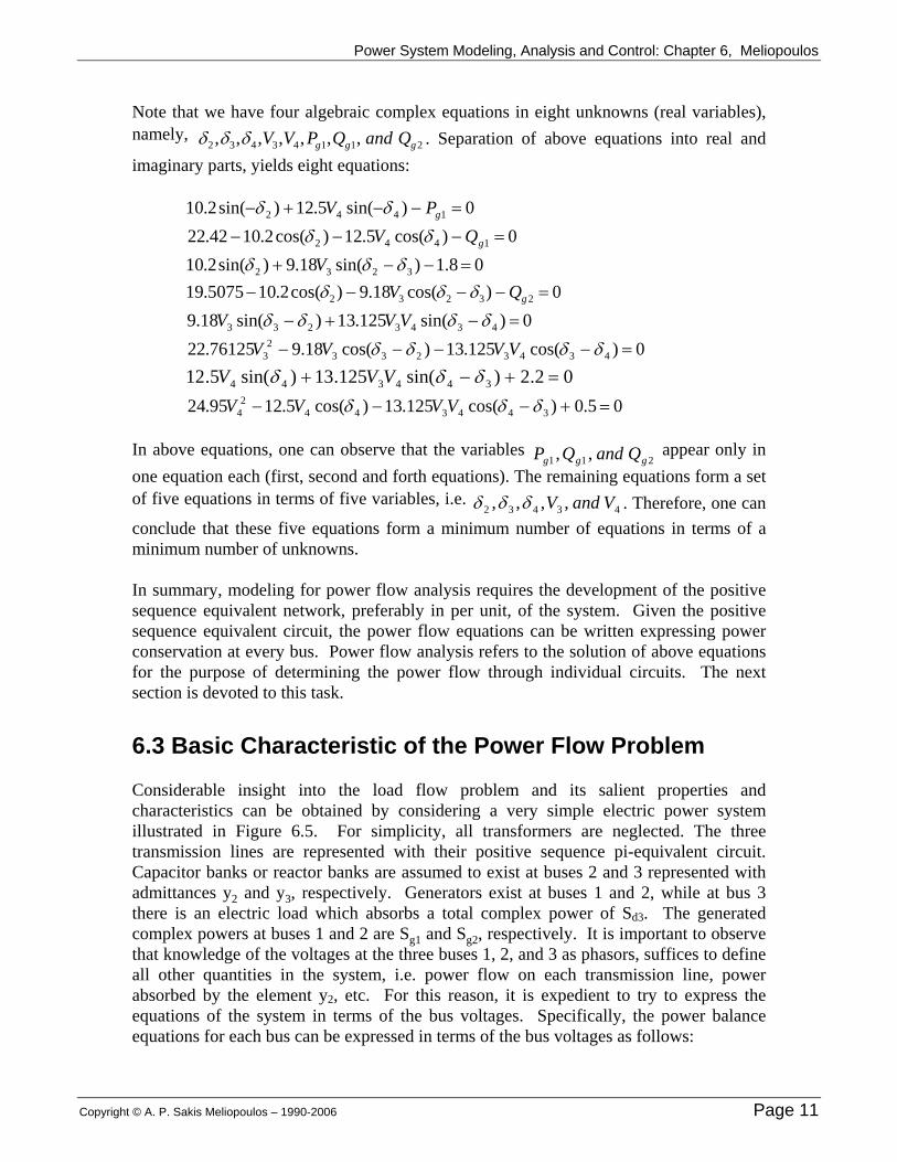
Note that we have four algebraic complex equations in eight unknowns (real variables), namely,
21143432 ,,,,,,, ggg QandQPVVδδδ . Separation of above equations into real and imaginary parts, yields eight equations: 0)sin(5.12)sin(2.10 1442 =−−+− gPV δδ 0)cos(5.12)cos(2.1042.22 1442 =−−− gQV δδ 08.1)sin(18.9)sin(2.10 3232 =−−+ δδδ V 0)cos(18.9)cos(2.105075.19 23232 =−−−− gQV δδδ 0)sin(125.13)sin(18.9 4343233 =−+− δδδδ VVV 0)cos(125.13)cos(18.976125.22 4343233
23 =−−−− δδδδ VVVV
02.2)sin(125.13)sin(5.12 344344 =+−+ δδδ VVV 05.0)cos(125.13)cos(5.1295.24 344344
24 =+−−− δδδ VVVV
In above equations, one can observe that the variables appear only in one equation each (first, second and forth equations). The remaining equations form a set of five equations in terms of five variables, i.e.
211 ,, ggg QandQP
43432 ,,,, VandVδδδ . Therefore, one can conclude that these five equations form a minimum number of equations in terms of a minimum number of unknowns. In summary, modeling for power flow analysis requires the development of the positive sequence equivalent network, preferably in per unit, of the system. Given the positive sequence equivalent circuit, the power flow equations can be written expressing power conservation at every bus. Power flow analysis refers to the solution of above equations for the purpose of determining the power flow through individual circuits. The next section is devoted to this task.
6.3 Basic Characteristic of the Power Flow Problem Considerable insight into the load flow problem and its salient properties and characteristics can be obtained by considering a very simple electric power system illustrated in Figure 6.5. For simplicity, all transformers are neglected. The three transmission lines are represented with their positive sequence pi-equivalent circuit. Capacitor banks or reactor banks are assumed to exist at buses 2 and 3 represented with admittances y2 and y3, respectively. Generators exist at buses 1 and 2, while at bus 3 there is an electric load which absorbs a total complex power of Sd3. The generated complex powers at buses 1 and 2 are Sg1 and Sg2, respectively. It is important to observe that knowledge of the voltages at the three buses 1, 2, and 3 as phasors, suffices to define all other quantities in the system, i.e. power flow on each transmission line, power absorbed by the element y2, etc. For this reason, it is expedient to try to express the equations of the system in terms of the bus voltages. Specifically, the power balance equations for each bus can be expressed in terms of the bus voltages as follows:
Copyright © A. P. Sakis Meliopoulos – 1990-2006 Page 11

Power System Modeling, Analysis and Control: Chapter 6, Meliopoulos
0~~~~~
11*
3*
131*
2*
121
2
1*
11 =+−++ dg SSVYVVYVVY (6.3a)
0~~~~~22
*3
*232
2
2*
22*
1*
212 =+−++ dg SSVYVVYVYV (6.3b)
0~~~~~3
2
3*
33*
2*
323*
1*
313 =+++ dSVYVYVVYV (6.3c)
where: Y11 = y12 + yS12 + y13 + yS13 Y12 = Y21 = -y12 Y13 = Y31 = -y13 Y22 = y2 + y12 + yS12 +y23 + yS23 Y23 = Y32 = y23 Y33 = y3 + y13 + yS31 + y23 + yS32
Sd3
2
G1 G2
Sd2
Sd1
1
3
y
y yy
y
y
yy
y
y
12
s12 s21
s13
s31
13 23
s32
s23
2
y3
S Sg1 g2
Figure 6.5 A Simple Three Bus Electric Power System
A number of variables appear in these equations. Dommel and Tinney [???] has suggested a classification of all variables in a way which is useful for formulating power flow problems and other related problems. It is expedient to introduce this classification and comment on the nature of these variables: System Parameter Variables. These are the line and transformer admittances, transformer taps, etc. In above equations they are included in the variables, Y11, Y12, etc. It is assumed that they are known. The parameters will be denoted with the vector p. Electric Power Demand Variables. These consist of all externally determined real and reactive loads of the system. For the system under consideration, they are Sd1 = Pd1 + jQd1, Sd2 = Pd2 + jQd2 and Sd3 = Pd3 + jQd3. These variables will be denoted with the vector d.
Page 12 Copyright © A. P. Sakis Meliopoulos – 1990-2006

Power System Modeling, Analysis and Control: Chapter 6, Meliopoulos
State Variables. The state variables are defined as the minimum set of variables, the knowledge of which will enable the computation of all relevant quantities of interest. In the case of the power flow problem, these variables are all the complex bus voltages. The complex bus voltages can be expressed in polar or rectangular coordinates. The polar representation of bus k voltage is utilized in this text given with kj
kk eVV δ=~
The voltage magnitude at certain buses is maintained at a specified value through generator excitation control or through regulating transformer action. At these buses only the phase of the voltage is considered to be a state variable. In addition, the phase variables, δk, are normally defined with respect to a certain time reference (see Chapter 2). Without loss of generality, we can select the time reference in such a way that the phase angle at an arbitrarily selected bus is zero. Later we will see that we normally select this bus to be a generation bus and we call this bus the slack bus. Thus, the state variables, which are denoted with the vector x, are the δk variables for all buses except the slack bus and a subset of the Vk variables. Control Variables. These consist of all quantities that can be independently manipulated or by existing control loops to satisfy system objectives. For the power flow problem, these are:
• Voltage magnitude at certain buses. For example, generation buses, buses connected to regulating transformers, or buses with synchronous condensers, etc.
• Real power generation at generation buses. (This controls are not totally independent since at all times the total generation must equal the system load plus losses)
• Tap settings of transformers. • Phase shift of phase shifting transformers • Switch status of capacitor and/or reactor banks (open/close). • Etc.
The control variables are denoted with the vector u. In summary, the variables appearing in the power flow equations have been classified into parameters (p), demand variables (d), state variables (x), and control variables (u). It is important to note that there is no unique way of separating the variables into the defined groups. This classification is depended upon the application and formulation of the problem. For example, a transformer tap variable may be a parameter, a state, or a control variable depending on system operation options. Now examine equations (6.3) with the objective of revealing the essence of the power flow analysis. First of all, the objective is to compute the electric power flow in each circuit of the system, the voltage level at every bus, etc. Observe that, in general, a
Copyright © A. P. Sakis Meliopoulos – 1990-2006 Page 13

Power System Modeling, Analysis and Control: Chapter 6, Meliopoulos
number of variables in equations (6.3) will be specified. For example, the real power of generator G2 output, the voltage magnitude at bus 1, etc. In general, the following parameters are associated with each bus, k, in the system: Sgk: electric power generated at bus k consisting of real and reactive power: Sgk = Pgk + jQgk Sdk: electric power consumed at bus k consisting of real and reactive power: Sdk = Pdk + jQdk V~
k: voltage at bus k. This is a phasor, with magnitude Vk and phase δk. Thus at each bus a total of six variables may be defined. On the other hand, at each bus one complex equation must be satisfied (complex power balance equation) or two equations in real variables (real power flow balance equation and reactive power balance equation). In order to match the number of equations to the number of unknown variables, only two out of six variables at a bus may be unknown. Note that a subset of the six variables at a bus will be specified by operator action or power system control actions, for example generation excitation control. It is expected that the unknown variables and equations (6.3) represent a consistent system of equations, i.e., the number of equations equals the number of unknowns. An examination of equation (6.3) reveals quickly that the arbitrary selection of both generators complex power outputs is not feasible. Since the sum of the generator real power output should always equal the real power load plus losses and since the system losses are not a priori known, one of the generators should be allowed to adjust its real power output. This generator takes the slack due to the yet uncalculated system losses. According to the generally accepted terminology, the bus to which this generator is connected to is called the slack bus. The inherent assumption here is that the available generation at the slack bus is large enough to take the “slack”. It is also assumed that the generators at the slack bus control the voltage magnitude of this bus. Thus the magnitude of the voltage at the slack bus is specified. In addition, without loss of generality, the phase of this voltage can be assumed to be equal to zero (see previous discussion). Thus:
specifiedVeVV j1
0.011 ,~ =
The specification of the voltage V1 results in decoupling equation (6.3a) from (6.3b) and (6.3c). This means that equations (6.3b) and (6.3c) can be solved independently from (6.3a). Then, the solution is utilized to compute the slack bus generation with equation (6.3a). This property carries to large electric power systems as well. The preceding discussion reveals that, mathematically, the power flow problem for the system under consideration collapses to the simultaneous solution of equations (6.3b) and (6.3c).
Page 14 Copyright © A. P. Sakis Meliopoulos – 1990-2006

Power System Modeling, Analysis and Control: Chapter 6, Meliopoulos
Similarly, the buses of the system can be classified according to the type of known variables associated with them. Recall that at each bus six variables can be defined. These six variables appear in the power balance equations of a bus in terms of the following four quantities: l) Real power injection Pk = Pgk - Pdk 2) Reactive power injection Qk = Qgk - Qdk 3) Voltage magnitude Vk 4) Voltage phase angle δk. The following definitions are useful in the formulation of the power flow problem. Slack Bus. The bus of the system for which the real and reactive power are allowed to swing (or take the “slack”) and for which the voltage phase angle is specified to be zero. Most common, the voltage magnitude at this bus is also specified. PQ Bus. Any bus for which the real power injection (Pk) and the reactive power injection (Qk) are specified (or known). PV Bus. Any bus for which the real power injection (Pk) and the voltage magnitude (Vk) are specified. With reference to Figure 6.5, bus 1 is the slack bus, bus 2 is a PV bus, and bus 3 is a PQ bus. From above analysis, it is obvious that a PQ bus contributes two state variables (the voltage magnitude and the phase, Vk and δκ, respectively), while a PV bus contributes one state variable only (the phase of the voltage δκ). Now consider equations (6.3b) and (6.3c). Expressing the voltages in polar form and separating real and imaginary parts, the following four equations are obtained
0)( 223,1
223,1
2222
2 =+−−⎥⎦
⎤⎢⎣
⎡++ ∑∑
==dg
mmm
mmsm PPVVgggV α (6.4a)
0)( 223,1
223,1
2222
2 =+−−⎥⎦
⎤⎢⎣
⎡++− ∑∑
==dg
mmm
mmsm QQVVbbbV β (6.4b)
0)( 32,1
332,1
3332
3 =+−⎥⎦
⎤⎢⎣
⎡++ ∑∑
==d
mmm
mmsm PVVgggV α (6.4c)
0)( 32,1
332,1
3332
3 =+−⎥⎦
⎤⎢⎣
⎡++− ∑∑
==d
mmm
mmsm QVVbbbV β (6.4d)
where kmkmkm jbgy += skmskmskm jbgy +=
kkk jbgy +=
Copyright © A. P. Sakis Meliopoulos – 1990-2006 Page 15

Power System Modeling, Analysis and Control: Chapter 6, Meliopoulos
)sin()cos( mkkmmkkmkm bg δδδδα −+−= )cos()sin( mkkmmkkmkm bg δδδδβ −−−= Careful inspection of the above four equations reveals that the following unknowns appear in these equations: First equation: δ2, V3, δ3 Second Equation: (Qg2 - Qd2), δ2, V3, δ3 Third equation: δ2, V3, δ3 Fourth equation: δ2, V3, δ3 Obviously, the second equation is decoupled from the remaining equations in the sense that it introduces a new unknown (Qg2 - Qd2) which does not appear in the other equations. The first, third, and fourth equations form a set of three equations in three unknowns only, namely δ2, V3, δ3. Note that according to the definitions, these three variables form the state variables. The procedure has isolated three equations (first, third, and fourth equation) and an equal number of state variables δ2, V3, δ3. These equations provide the formulation of the power flow problem for this system and they are summarized below.
0)( 223,1
223,1
2222
2 =+−−⎥⎦
⎤⎢⎣
⎡++ ∑∑
==dg
mmm
mmsm PPVVgggV α (6.4a)
0)( 32,1
332,1
3332
3 =+−⎥⎦
⎤⎢⎣
⎡++ ∑∑
==d
mmm
mmsm PVVgggV α (6.4c)
0)( 32,1
332,1
3332
3 =+−⎥⎦
⎤⎢⎣
⎡++− ∑∑
==d
mmm
mmsm QVVbbbV β (6.4d)
This procedure can be generalized to large electric power systems. The generalization is presented in the next section.
6.4 Power Flow Problem Formulation for Large Systems The analysis of the previous paragraph and the introduced definitions allow the formulation of the load flow problem for large electric power systems. Note that the procedure requires (a) the power balance equations at the buses of the system, and (b) selecting a proper subset of these equations which will provide the minimum number of simultaneous equations in terms of an equal number of state variables (equal number of equations and unknowns). The solution of these equations provides the system state. A systematic way of writing the power flow equations for any bus is given below, followed by the selection process. The power flow equations can be developed with reference to Figure 6.6 illustrating a general bus k of a large electric power system. A
Page 16 Copyright © A. P. Sakis Meliopoulos – 1990-2006

Power System Modeling, Analysis and Control: Chapter 6, Meliopoulos
circuit between any two buses k,m is represented with its equivalent positive sequence pi-equivalent circuit. In general, one or more circuits may be connected to a bus. In addition, an admittance yk may be also connected to a bus (a capacitor, a reactor, etc.). It is assumed that electric current Igk is injected to bus k from the generators connected to this bus. Also, electric current Idk is absorbed from the electric load connected to this bus. In general, one or both of these currents may be absent from a bus. The voltage of bus k is assumed to be V
~k and the voltage of bus m, V
~m. Electric current will flow
through the circuit k,m as it is indicated in Figure 6.6. This electric current will be: mkmkskmkmkm VyVyyI ~~)(~ −+= (6.5) In case a capacitor bank or a reactor is connected to bus k, of admittance yk, the electric current absorbed by this admittance will be kkVy ~
k. Similarly, all other electric currents on the circuits connected to bus k can be computed. Application of Kirchoff's current law to bus k will yield: (6.6) ∑
∈
+=−)(
~~~~kKm
kmkkdkgk IVyII
where K(k) represents the set of buses which share a circuit with bus k. Upon substitution of I
~km:
(6.7) ∑∑∈∈
−⎟⎟⎠
⎞⎜⎜⎝
⎛++=−
)()(
~~)(~~kKm
mkmkkKm
kmskmkdkgk VyVyyyII
Define ∑
∈
++=)(
)(kKm
kmskmkkk yyyY
kmkm yY −= and recognize that Ykk and Ykm are the elements (kth diagonal and (k,m)th element, respectively) of the usual admittance matrix of the power system network. Now equation (6.7) assumes the form: (6.8) ∑
∈
+=−)(
~~~~kKm
mkmkkkdkgk VYVYII
Copyright © A. P. Sakis Meliopoulos – 1990-2006 Page 17

Power System Modeling, Analysis and Control: Chapter 6, Meliopoulos
Nonlinear
bus k bus m
Igk
Idk
Electric Load
yk
yskm
ysmk
ykm
To Other Circuits
Ikm
Linear
Figure 6.6 Symbolic Representation of a General Bus of an Electric Power System - Positive Sequence Network
In power flow studies, the known (or specified or measured) quantities are usually the electric power generated at a bus and/or the electric power absorbed by the load. These quantities for bus k will be designated with Sgk, Sdk, respectively, and are equal to: *~~
gkkgk IVS = (6.9) (6.10) *~~
dkkdk IVS = where the asterisk denotes complex conjugation. The total electric power injected to a bus is obviously Sgk - Sdk. Combination of equations (6.8), (6.9), and (6.10) yields: Sgk - Sdk = Y*kk Vk
2 + V~
k ∑m∈Κ(k)
Y*km V~
*m (6.11)
In general , , kj
kk eVV δ=~mj
mm eVV δ=~
kkk jbgy += kmkmkm jbgy += skmskmskm jbgy += Upon substitution of above relationships into equation (6.11)
Page 18 Copyright © A. P. Sakis Meliopoulos – 1990-2006

Power System Modeling, Analysis and Control: Chapter 6, Meliopoulos
))(j-)()()(
2
)()(
2 ∑∑∑∑∈∈∈∈
−⎥⎦
⎤⎢⎣
⎡++−⎥
⎦
⎤⎢⎣
⎡++=−
kKmmkmk
kKmskmkmkk
kKmmkmk
kKmskmkmkkdkgk VjVbbbVVVgggVSS βα (6.12)
where: )sin()cos( mkkmmkkmkm bg δδδδα −+−= )cos()sin( mkkmmkkmkm bg δδδδβ −−−= Finally by separating above equation into real and imaginary parts:
(6.13a) ∑∑∈∈
−⎥⎦
⎤⎢⎣
⎡++=−
)()(
2 )(kKm
mkmkkKm
skmkmkkdkgk VVgggVPP α
(6.13b) ∑∑∈∈
−⎥⎦
⎤⎢⎣
⎡++−=−
)()(
2 )(kKm
mkmkkKm
skmkmkkdkgk VVbbbVQQ β
Equation (6.12) or its expended form (6.13) expresses power conservation at bus k: the injected electric power Sgk - Sdk equals the electric power flowing to the circuits. For an electric power system comprising n buses, n such equations can be written; one for each bus. These n equations are called the power balance equations. Observe that in a power system comprising n buses, and assuming that m of the n buses are PQ buses, the minimum set of variables describing the state of the system are:
• The phase of bus voltages at all buses except the slack bus; nδδδ ...,,, 32 . • The voltage magnitude at all PQ buses; where k
qkkk VVV ...,,,21 1 is the first PQ
bus, ..., kq is the last PQ bus. These variables are the state variables x. Thus, the state vector comprises n-1+q unknown variables. The state vector will be determined from an appropriate set of n-1+q independent equations. For the purpose of selecting these equations, observe the following: The real power equation for a PV bus expresses the relationship among the real power injection at this bus to the state vector x. Also, the reactive power equation for a PQ bus expresses the relationship among the known reactive power injection at this bus to the state vector x. Consider the following equations: (a) n-1 real power balance equations; one for each bus except the slack bus (b) q reactive power balance equations; one for each PQ bus; These equations are independent. The only unknowns appearing in these equations are the voltages phases nδδδ ...,,, 32 , and the voltage magnitudes (state variables, a total of n-1+q unknowns). The simultaneous solution of this system of equations will provide the state vector x and thus, the solution to the power flow problem. This set of equations are the
qkkk VVV ...,,,21
power flow equations.
Copyright © A. P. Sakis Meliopoulos – 1990-2006 Page 19

Power System Modeling, Analysis and Control: Chapter 6, Meliopoulos
In order to facilitate notation and symbolism, the following convention will be applied. It is assumed that the slack bus is bus number 1. Then the equations are numbered as follows: The first equation will be the real power equation for bus 2, the second will be the real power equation for bus 3, etc. The (n-l)th equation will be the real power equation for bus n. The nth equation will be the reactive power equation for bus k1 (first PQ bus), etc. The (n-1+q)th equation will be the reactive power equation for bus kq (last PQ bus). This numbering of equations determines the numbering of the state variables. Specifically, the first state variable is δ2 the second state variable is δ3, etc, the (n-l)th state variable is δn, the nth state variable is , etc., and the (n-1+q)th state variable is
. 1kV
qkV The determination of a minimum set of equations in equal number of unknowns for the solution of the load flow problem is illustrated with an example. Example E6.3: For the system of Figure E6.1b write the power flow equations, i.e. a minimum set of equations in equal number of unknowns) whose solution will provide the power flow solution. Solution: The state variables are two: δ2 and V2. The two equations are g1(x) = 5.05V2sin δ2 + 0.85 = 0 g2(x) = 5 - 5.05VV2
22cos δ2 + 0.36 = 0
Example E6.4: For the system of Figure E6.2, write the power flow equations, i.e. a minimum set of equations whose solution will provide the power flow solution. Solution: The state variables are five, δ2, δ3, δ4, V3, V4. The five equations which will provide the solution are: Three real power equations, one each for buses 2, 3, 4; two reactive power equations, one each for buses 3, 4. 8.1)sin(18.9)sin(2.10)( 32321 −−+= δδδ Vxg )sin(125.13)sin(18.9)( 43432332 δδδδ −+−= VVVxg 2.2)sin(125.13)sin(5.12)( 3443443 +−+= δδδ VVVxg
)cos(125.13)cos(18.976125.22)( 43432332
33 δδδδ −−−−= VVVVxg5.0)cos(125.13)cos(5.1295.24)( 344344
245 +−−−= δδδ VVVVxg
Note that assuming that the state variables δ2 δ3, δ4 and V3, V4 have been computed, other quantities of interest, such as Qg2, Pg1, and Qg1 can be computed by direct substitution into the equations: )cos(18.9)cos(2.105075.19 32322 δδδ −−−= VQg )sin(5.12)sin(2.10 4421 δδ −+−= VPg
Page 20 Copyright © A. P. Sakis Meliopoulos – 1990-2006

Power System Modeling, Analysis and Control: Chapter 6, Meliopoulos
)cos(5.12)cos(2.1042.22 4421 δδ VQg −−=
6.5 Solution Techniques The formulation of the power flow problem leads to a system of nonlinear algebraic equations. Solution of these equations can be obtained with a number of numerical analysis algorithms which shall be reviewed in this section. The discussion will be confined only to algorithms which have been successfully applied to the power flow problem. In general, the power flow equations can be written in the following general form: 0),,( =upxg (6.14) where x is the state vector p is the parameter vector u is the control vector g is the set of power flow equations. For the power flow problem, it is assumed that the vectors p and u are known or specified, in which case the equations are written as (6.15) 0)( =xg In expanded form, the above vector equation reads: g1 (x1, x2, ... , xn) = 0 g2 (x1, x2, ... , xn) = 0 (6.16) . . . . . . . . . . . . . . . . gn (x1, x2, ... , xn) = 0 The solution of the nonlinear set of equations (6.15) can be obtained with an algorithm of the general form [???]: (6.17) )(1 ννν xAxx +=+
where is the state vector at iteration νx ν . A is the algorithm which transforms a given state vector into . νx )( νxA
Copyright © A. P. Sakis Meliopoulos – 1990-2006 Page 21

Power System Modeling, Analysis and Control: Chapter 6, Meliopoulos
The algorithm A should be selected in such a way as to provide the correct solution x by repetitive application of equation (6.17). This section is devoted to the algorithms (6.17) and their practical implementation to the power flow problem. The algorithms applied to the power flow problem can be classified into two broad categories, (a) coordinate methods and (b) gradient methods. Table 6.1 lists these categories. The two categories of solution methods will be briefly discussed.
Table 6.1 Numerical Solution Techniques Applied to the Power Flow Problem
Class A Class B
Coordinate Methods Gradient Methods * Gauss Method
* Gauss/Seidel Method * Optimal Descent * Newton/Raphson
* Quasi Newton Methods
6.5.1 Coordinate Methods The idea of this method is very simple and it is credited to Gauss. Given a set of n equations in n unknowns, solve equation 1 for unknown #1, then solve equation #2 for unknown 2, etc., until the last equation. It can be easily proven, that this procedure is always possible assuming that the n equations are independent. Completion of above procedure transforms, equation (6.15) into equation (6.18) below: x = G(x) (6.18) The algorithm is now defined in terms of the function G(x): )( νxA (6.19) ννν xxGxA −= )()( )(1 ννν xAxx +=+
The coordinate method is illustrated with an example. Example E6.5: Solve the following set of equations using the coordinate method. 10x1 - 2x2 - 1 = 0 -x1 + 100x2 - 2 =0 Solution: Solve first equation for x1, and second equation for x2 x1 = 0.1 + 0.2x2
Page 22 Copyright © A. P. Sakis Meliopoulos – 1990-2006
Power System Modeling, Analysis and Control: Chapter 6, Meliopoulos
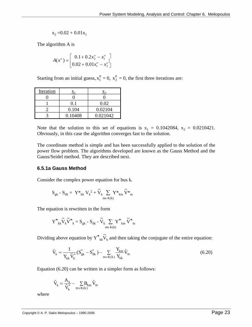
x2 =0.02 + 0.01x1 The algorithm A is
⎥⎦
⎤⎢⎣
⎡
−+−+
= υυ
υυυ
21
12
01.002.02.01.0
)(xx
xxxA
Starting from an initial guess, = 0, x = 0, the first three iterations are: x1
020
Iteration x1 x2
0 0 0 1 0.1 0.02 2 0.104 0.02104 3 0.10408 0.021042
Note that the solution to this set of equations is x1 = 0.1042084, x2 = 0.0210421. Obviously, in this case the algorithm converges fast to the solution. The coordinate method is simple and has been successfully applied to the solution of the power flow problem. The algorithms developed are known as the Gauss Method and the Gauss/Seidel method. They are described next. 6.5.1a Gauss Method Consider the complex power equation for bus k. Sgk - Sdk = Y*kk Vk
2 + V~
k ∑m∈Κ(k)
Y*km V~
*m
The equation is rewritten in the form Y*
kkV~
kV~*
k = Sgk - Sdk - V~
k ∑m∈Κ(k)
Y*km V
~*m
Dividing above equation by Y*
kkV~
k and then taking the conjugate of the entire equation:
%%
( ) %*
* *
( )V
Y VS S Y
YVk
kk kgk dk
km
kkm K km= − − ∑
∈
1 (6.20)
Equation (6.20) can be written in a simpler form as follows:
%%
%*
( )V A
VB Vk
k
kkm
m K km= − ∑
∈
where
Copyright © A. P. Sakis Meliopoulos – 1990-2006 Page 23

Power System Modeling, Analysis and Control: Chapter 6, Meliopoulos
Ak = (Sgk
* - Sdk*) / Ykk
Bkm = Ykm / Ykk K(k) is the set of buses connected to bus k. In summary, the Gauss method is expressed with the algorithm:
nkVBVA
VkKm
mkmk
kk ...,,2,1,~
~~
)(
1 =−= ∑∈
+ νν
ν (6.21)
If voltage control buses exist in the system, the algorithm for these buses must change to reflect the fact that the voltage magnitude is controlled. The required changes are very simple. After each iteration of the algorithm, the voltage magnitude of the voltage controlled buses are set to the specified values. 6.5.1b Gauss/Seidel Method This method is an extension of the Gauss method. The basic idea is to employ the most recent values of the voltage variables in the application of the algorithm. Thus, the algorithm of equation (6.21) is modified to
υυυ
υm
kmkKmkmm
kmkKmkm
k
kk VBVB
V
AV ~~
~~
),(
1
),(*
1 ∑∑>∈
+
<∈
+ −−= , k = 2, 3, ..., n (6.22)
The voltage controlled buses are treated in the same way as in the Gauss method. The Gauss or Gauss/Seidel method will be demonstrated with an example. Example E6.6: Consider the simplified electric power system of Figure E6.1, Example E6.1. For this system: (a) Develop the Gauss/Seidel algorithm (b) Perform four iterations of the algorithm assuming the following initial guess: (a) all
unspecified voltage magnitudes equal to 1.0 pu, (b) all unspecified phase angles equal to 0.0.
Solution: a) The Gauss algorithm is:
υυ
υ121*
2
212
~~
~ VBV
AV −=+
where 17.0072.00.5
36.085.0
22
*2
*2
2 jj
jY
SSA dg −−=
−−
=−
=
Page 24 Copyright © A. P. Sakis Meliopoulos – 1990-2006

Power System Modeling, Analysis and Control: Chapter 6, Meliopoulos
0.10.5
0.5
22
2121 −=
−==
jj
YY
B
Therefore:
01.1~17.0072.0~
*2
12 +
−−=+
νν
VjV
b) Four iterations of the algorithm starting from V
~2 = 1.0 :
Iteration # Voltage V
~2
0 1.0 1 0.9532e-j10.27o
2 0.9183e -j10.16o
3 0.9158e -j10.60o
4 0.9142e-j10.59o
6.5.2 Gradient Methods Gradient methods is a general class of numerical algorithms for the solution of a set of nonlinear equations. The name is attributed to the fact that at each iteration, the solution moves along the gradient of the equations at the present solution. Thus, (6.23) )(1 ννν α xdxx +=+
where present solution νx the gradient at the present solution, )( νxd νx α a scalar appropriately selected. There are many variations of gradient methods. The most widely used are listed in Table 6.2. The convergence properties of the methods are also listed.
Table 6.2 Gradient Methods
Optimal Descent Newton's Method Quasi Newton d(xυ)* ∇g J-1 g(x) C g(x)
α* Optimal -1 -1 Convergence Speed First Order Quadratic Near Quadratic
*General Algorithm: )(1 ννν α xdxx +=+
All of above methods have been successfully employed to the problems of power flow, optimal power flow and other analysis problems. The optimal descent method has not
Copyright © A. P. Sakis Meliopoulos – 1990-2006 Page 25

Power System Modeling, Analysis and Control: Chapter 6, Meliopoulos
been widely accepted because its poor convergence characteristics. The Newton's method and Quasi-Newton methods have emerged as the preferred methods for power flow analysis. In subsequent sections, these methods will be presented with applications to the power flow problem. 6.5.2a Newton's Method Direct application of Newton's numerical solution algorithm to the power flow equations, as developed in previous sections, is known as the Newton/Raphson method. Newton's method will be reviewed first in its general form and then applied to the power flow equations. Consider the system of nonlinear equations (6.15) which in expended form are shown as equations 6.16 and which are repeated here: g1 (x1, x2, ... , xn) = 0 g2 (x1, x2, ... , xn) = 0 (6.24) . . . . . . . . . . . . . . . . . gn (x1, x2, ... , xn) = 0 Assume that estimates xl
0, x20,..., xn
0 for the n variables are known. Further assume that these estimates do not satisfy equations (6.24) and, thus, a better estimate is necessary. Newton's method provides the means by which this new better estimate can be obtained. For this purpose, the functions g1, g2, ..., gn are linearized around the known estimate of x0, (xl
0, x20,..., xn
0 ). The procedure yields:
...)(),...,(),...,( 0
1
1002
011211 tohxx
xg
xxxgxxxg ii
n
i inn +−+= ∑
= ∂∂
...)(),...,(),...,( 0
1
2002
012212 tohxx
xg
xxxgxxxg ii
n
i inn +−+= ∑
= ∂∂
. . . . . . . . . . . . . . .. . . . . . . . . .
...)(),...,(),...,( 0
1
002
0121 tohxx
xg
xxxgxxxg ii
n
i i
nnnnn +−+= ∑
= ∂∂
In above expression, h.o.t. stands for higher order terms. Assuming that the actual solution x is very close to the guess x0 , then the higher order terms will be negligible because they depend on terms (xi - xi
o)m where m ≥ 2. Thus neglecting the higher order terms, the following equations are obtained:
.0.0)(),...,( 0
1
1002
011 ≅−+ ∑
=ii
n
i in xx
xg
xxxg∂∂
.0.0)(),...,( 0
1
2002
012 ≅−+ ∑
=ii
n
i in xx
xg
xxxg∂∂
Page 26 Copyright © A. P. Sakis Meliopoulos – 1990-2006

Power System Modeling, Analysis and Control: Chapter 6, Meliopoulos
. . . . . . . . . . . . . . .. . . . . . . . . .
.0.0)(),...,( 0
1
002
01 ≅−+ ∑
=ii
n
i i
nnn xx
xg
xxxg∂∂
In compact matrix notation above equations read:
0)()( 00 =−⎥⎦⎤
⎢⎣⎡+ xx
xgxg
∂∂ (6.25)
where
, ,
⎥⎥⎥⎥⎥
⎦
⎤
⎢⎢⎢⎢⎢
⎣
⎡
=
03
02
01
0
x
xx
xM
⎥⎥⎥⎥⎥
⎦
⎤
⎢⎢⎢⎢⎢
⎣
⎡
=
),...,,(
),...,,(),...,,(
)(
002
01
002
012
002
011
0
nn
n
n
xxxg
xxxgxxxg
xgLL
and
⎥⎥⎥⎥⎥⎥⎥⎥
⎦
⎤
⎢⎢⎢⎢⎢⎢⎢⎢
⎣
⎡
=
n
nnn
n
n
xg
xg
xg
xg
xf
xg
xg
xg
xg
xg
∂∂
∂∂
∂∂
∂∂
∂∂
∂∂
∂∂
∂∂
∂∂
∂∂
L
LLLL
L
L
21
2
2
2
1
2
1
2
1
1
1
The matrix ∂∂gx
, can be recognized to be the Jacobian matrix of the functions g,
computed at x0 and will be symbolized with J(x0). Equation (6.25) is solved for the vector x yielding: (6.26) )()( 0010 xgxJxx −−= By construction, the vector x is a better estimate of the solution than vector x0. The procedure can be applied to any vector xυ yielding the following algorithm: (6.27) )()(11 νννν xgxJxx −+ −= The algorithm should terminate whenever a vector xυ has been found which makes the vector function very small. Note that in this case, equations (6.24) are satisfied. In summary, the solution to a set of nonlinear equations (6.24) can be obtained with the following steps:
)( νxg
Step 1: Assume an initial guess for x : x0. Let 0=ν .
Copyright © A. P. Sakis Meliopoulos – 1990-2006 Page 27

Power System Modeling, Analysis and Control: Chapter 6, Meliopoulos
Step 2: Compute . If || || ≤ ε , then is the solution. In this case, terminate. Otherwise, go to step 3.
)( νxg )( νxg νx
Step 3: Compute the Jacobian matrix . )( νxJ Compute [ ])()(11 νννν xgxJxx −+ −= . Let 1+=νν and go to step 2. The convergence characteristics of Newton's method have been extensively studied. It can be proven that the method possesses quadratic convergence. This means that near the solution, the following will be valid between two successive iterations: [ 21 )(()( υυ xgMxg ≅+ ] (6.28) where • indicates the norm of the argument, i.e. 2/122
221 ))(......)()(()( xgxgxgxg n+++=
and M is a finite number. This means that if at an iteration ν , the norm of the vector g(xυ) is in the order of 0.01, the norm of the vector g(xυ+1) will be in the order of 0.0001, the norm of the vector g(xυ+2) will be in the order of 0.00000001, etc. Example E6.7: Solve the following equation via Newton's method x + 2x2 + 3x4 - 0.5 = 0 Solution: Define g(x) = x + 2x2 + 3x4 - 0.5 Then [ ])()(11 νννν xgxJxx −+ −= where: J(x) = 1 + 4x + 12x3 Following are three iterations of the algorithm starting from x = 0.0
Iteration # xυ Function g(xυ) Jacobian J(xυ) 0 0.0 -0.5 1.0 1 0.5 0.6875 4.5 2 0.3472 0.1319 2.8911 3 0.3016 0.0083 2.5356 4 0.2983 0.000028 2.5117
In above example, one can observe the quadratic convergence characteristics of Newton’s method by studying the values . )( νxg
Page 28 Copyright © A. P. Sakis Meliopoulos – 1990-2006

Power System Modeling, Analysis and Control: Chapter 6, Meliopoulos
6.5.2b The Newton-Raphson Method in Polar Form The direct application of Newton's method to the solution of the power flow equations is known as the Newton-Raphson method. Depending on the form of the power flow equations, the method can be developed in polar coordinate form where bus voltages are expressed in polar coordinate form, i.e. magnitude and phase angle, or rectangular coordinate form. The most popular formulation is the polar coordinate form. The analysis of Section 6.4 indicates that the power flow problem is mathematically formulated as the solution of n-1+q nonlinear equations. These equations are the n-1 real power equations and q reactive power equations (q is the number of PQ buses). Assuming that bus 1 is always the slack bus, the following convention is adapted: The first equation is the real power equation for bus 2. The second equation is the real power equation for bus 3. ................................................... The (n - l)th equation is the real power equation for bus n. The nth equation is the reactive power equation for first PQ bus. ................................................... The (n-1+q)th equation is the reactive power equation for last PQ bus. In compact form, these equations can be written as 0),()( =−= ppp bVfxg δ (6.29a) 0),()( =−= qqq bVfxg δ (6.29b) where bp is an (n - l) x 1 vector of real power injections at buses 2, 3, ..., n bq is an q x 1 vector of reactive power injections at the PQ buses fp(δ,V) (n -1) functions of real power flow fq(δ,V) q functions of reactive power flow δ is an (n-l) x 1 vector of unknown voltage phases V is an q x 1 vector of unknown voltage magnitudes (at the PQ buses)
is the state vector. ⎥⎦
⎤⎢⎣
⎡=
Vx
δ
Direct application of Newton's method on these equations yields:
⎥⎥⎦
⎤
⎢⎢⎣
⎡
−−
⎥⎥⎥⎥
⎦
⎤
⎢⎢⎢⎢
⎣
⎡
∂
∂
∂
∂∂
∂
∂
∂
−⎥⎦
⎤⎢⎣
⎡=⎥
⎦
⎤⎢⎣
⎡
−
+
+
pp
pp
bVfbVf
VffVff
VV ),(),(
1
1
1
υυ
υυ
υ
υ
υ
υ
δδ
δ
δδδ (6.30)
Copyright © A. P. Sakis Meliopoulos – 1990-2006 Page 29

Power System Modeling, Analysis and Control: Chapter 6, Meliopoulos
The elements of the Jacobian matrix are computed by direct differentiation of the power flow equations. The form of the Jacobian depends on the selected form of the power equations. Table 6.3 tabulates the form of the power equations and associated Jacobian. when bus voltages are expressed in polar coordinate form and system admittances in rectangular coordinate form (hybrid form) the notation in Table 6.3 is consistent with Figure 6.6. Some of the most popular implementations of power flow algorithms are based on this form. In this textbook, the hybrid form will be adopted. The application of the method will be demonstrated with three examples. Example E6.8: Solve the power flow equations of example E6.1 with the Newton-Raphson method. Solution: The Newton-Raphson algorithm for this problem is
⎥⎦
⎤⎢⎣
⎡+−
+⎥⎦
⎤⎢⎣
⎡−
−⎥⎦
⎤⎢⎣
⎡=⎥
⎦
⎤⎢⎣
⎡ −
+
+
36.0cos05.5585.0sin05.5
cos05.510sin05.5sin05.5cos05.5
222
2
221
2222
222
2
21
2
12
δδ
δδδδδδ
υ
υ
υ
υ
VVV
VVV
VV
Starting with δ2 = 0, V2 = 1.0, the first three iterations are listed below: Iteration # δ2 V2 Vector g(x0) Jacobian
0 0 1.0 0 85
0 31..
⎡
⎣⎢⎤
⎦⎥
5 05 00 4 95.
.⎡
⎣⎢⎤
⎦⎥
1 -0.1683 0.9374 0 05700 0865..
⎡
⎣⎢⎤
⎦⎥
4 6668 0 84600 7930 4 3951. .. .
−−
⎡
⎣⎢⎤
⎦⎥
2 -0.1846 0.9147 0 00190 0029..
⎡
⎣⎢⎤
⎦⎥
4 5410 0 92710 8481 41833. .. .
−−
⎡
⎣⎢⎤
⎦⎥
3 -0.1852 0.9139 0 2504 100 3570 10
5
5. *. *
−
−
⎡
⎣⎢
⎤
⎦⎥
4 5365 0 93000 8500 41758. .. .
−−
⎡
⎣⎢⎤
⎦⎥
The solution above should be compared to the one obtained for the same system using Gauss method, i.e. Example E6.6. Example E6.9: Consider the simple two bus power system of Figure E6.9. The generator at bus 1 controls the voltage magnitude of bus 1 equal to 1.0 pu. When the capacitor bank switch is open, the voltage at bus 2 is V
~2 = 0.9e-j0.224 rad
Compute the voltage magnitude of bus 2 when the capacitor bank switch closes. Assume that the voltage magnitude at bus 1 is maintained at 1.0 pu. Use Newton's method and
Page 30 Copyright © A. P. Sakis Meliopoulos – 1990-2006

Power System Modeling, Analysis and Control: Chapter 6, Meliopoulos
perform one iteration. Also, compute the complex power of the generator unit before and after switching the capacitor.
S
1 2j0.1
= 2.0 + j0.6751.0ej0
-j2.0
G1
L1V =
All values are in pu
Figure E6.9 Solution: The power flow equations, when the capacitor switch closes, are: 10V2sinδ2 + 2.0 = 0 9.5V2
2 - 10V2cosδ2 + 0.675 = 0 The Newton/Raphson algorithm is
⎥⎦
⎤⎢⎣
⎡
+−+
⎥⎦
⎤⎢⎣
⎡
−−⎥
⎦
⎤⎢⎣
⎡=⎥
⎦
⎤⎢⎣
⎡−+
675.0cos105.90.2sin10
cos1019sin10sin10cos10
222
2
22
1
2222
222
2
21
2
2υυυ
υυ
υυυυ
υυυυυ
δδ
δδδδδδ
VVV
VVV
VV A good initial guess will be given by the condition prior to closing the switch, i.e. δ2
0 = -0.224 rads V2
0 = 0.9 pu Thus
⎥⎦
⎤⎢⎣
⎡−=⎥
⎦
⎤⎢⎣
⎡−⎥
⎦
⎤⎢⎣
⎡−
−−⎥
⎦
⎤⎢⎣
⎡−=⎥
⎦
⎤⎢⎣
⎡ −
95917.02090.0
405.00.0
35.7999.122.2775.8
9.0224.0 1
12
12
Vδ
The complex power generated by unit G1 prior to closing the switch is: Sg1
before = -10V2sinδ2 - j(10 - 10V2cosδ2) = 2.0 - j1.225 The complex power generated by unit G1 after the switch has closed is: Sg1
after = -10V2sinδ2 - j(10 - 10V2cosδ2) = 2.0 - j0.617 Thus the generated reactive power prior to the switching-in of the capacitor bank is -1.225 pu. It is reduced to -0.617 after switching-in the capacitor bank.
Copyright © A. P. Sakis Meliopoulos – 1990-2006 Page 31
Power System Modeling, Analysis and Control: Chapter 6, Meliopoulos
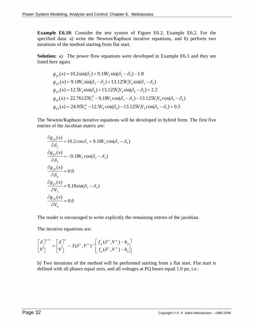
Example E6.10: Consider the test system of Figure E6.2, Example E6.2. For the specified data: a) write the Newton/Raphson iterative equations, and b) perform two iterations of the method starting from flat start. Solution: a) The power flow equations were developed in Example E6.3 and they are listed here again. 8.1)sin(18.9)sin(2.10)( 32321 −−+= δδδ Vxg p )sin(125.13)sin(18.9)( 43432332 δδδδ −+−= VVVxg p 2.2)sin(125.13)sin(5.12)( 3443443 +−+= δδδ VVVxg p
)cos(125.13)cos(18.976125.22)( 43432332
31 δδδδ −−−−= VVVVxgq
5.0)cos(125.13)cos(5.1295.24)( 3443442
42 +−−−= δδδ VVVVxgq
The Newton/Raphson iterative equations will be developed in hybrid form. The first five entries of the Jacobian matrix are:
)cos(18.9cos2.10)(
32322
1 δδδδ
−+=∂
∂V
xg p
)cos(18.9)(
3233
1 δδδ
−−=∂
∂V
xg p
0.0)(
4
1 =∂
∂
δxg p
)sin(18.9)(
323
1 δδ −=∂
∂
Vxg p
0.0)(
4
1 =∂
∂
Vxg p
The reader is encouraged to write explicitly the remaining entries of the jacobian. The iterative equations are:
⎥⎥⎦
⎤
⎢⎢⎣
⎡
−−
−⎥⎦
⎤⎢⎣
⎡=⎥
⎦
⎤⎢⎣
⎡ −+
pp
bVfbVf
VJVV ),(
),(),( 1
1
υυ
υυυυ
υυ
δδ
δδδ
b) Two iterations of the method will be performed starting from a flat start. Flat start is defined with all phases equal zero, and all voltages at PQ buses equal 1.0 pu, i.e.:
Page 32 Copyright © A. P. Sakis Meliopoulos – 1990-2006

Power System Modeling, Analysis and Control: Chapter 6, Meliopoulos
and ⎥⎥⎥
⎦
⎤
⎢⎢⎢
⎣
⎡=
⎥⎥⎥
⎦
⎤
⎢⎢⎢
⎣
⎡
=000
04
03
02
0
δδδ
δ ⎥⎦
⎤⎢⎣
⎡=⎥
⎦
⎤⎢⎣
⎡=
0.10.1
04
030
VV
V
1st Iteration: The following are computed upon substitution
⎥⎥⎥
⎦
⎤
⎢⎢⎢
⎣
⎡=
000
),( 00 Vf p δ
⎥⎦
⎤⎢⎣
⎡−
=1169.0
3952.0),( 00 Vf q δ
⎥⎥⎥⎥⎥⎥
⎦
⎤
⎢⎢⎢⎢⎢⎢
⎣
⎡
−−
−−−
−
=
1710.239048.110009048.118752.21000004048.249048.110009048.110848.211800.90001800.93800.19
),( 00 VJ δ
The inverse of the Jacobian matrix is:
⎥⎥⎥⎥⎥⎥
⎦
⎤
⎢⎢⎢⎢⎢⎢
⎣
⎡
=−
0599.0326.0000326.0635.000
000627.0446.0211.000446.0915.0433.000211.0433.0721.
),( 100 VJ δ
The power mismatch vector is
⎥⎥⎥⎥⎥⎥
⎦
⎤
⎢⎢⎢⎢⎢⎢
⎣
⎡
−
−
=⎥⎥⎦
⎤
⎢⎢⎣
⎡
−−
1169.03952.0
2.20.08.1
),(),(
00
00
pp
bVfbVf
δδ
Upon substitution of above values into the algorithm:
Copyright © A. P. Sakis Meliopoulos – 1990-2006 Page 33

Power System Modeling, Analysis and Control: Chapter 6, Meliopoulos
⎥⎥⎥⎥⎥⎥
⎦
⎤
⎢⎢⎢⎢⎢⎢
⎣
⎡
−−
=
⎥⎥⎥⎥⎥⎥
⎦
⎤
⎢⎢⎢⎢⎢⎢
⎣
⎡−
−
⎥⎥⎥⎥⎥⎥
⎦
⎤
⎢⎢⎢⎢⎢⎢
⎣
⎡
=⎥⎦
⎤⎢⎣
⎡
9941.09787.01000.0202.
0833.
0059.0213.1000.0202.0833.
0.10.1
000
1
1
Vδ
This completes the first iteration. 2nd Iteration: The following are computed
⎥⎥⎥⎥⎥⎥
⎦
⎤
⎢⎢⎢⎢⎢⎢
⎣
⎡−−
=⎥⎥⎦
⎤
⎢⎢⎣
⎡
−−
0983.00932.00361.00048.00228.0
),(),(
11
11
pp
bVfbVf
δδ
⎥⎥⎥⎥⎥⎥
⎦
⎤
⎢⎢⎢⎢⎢⎢
⎣
⎡
−−−−−−−−
−−−−
=
2439.237971.111639.29235.006145.111184.219235.00048.09283.01767.29435.09106.235462.110
9289.00049.05462.114829.209367.809484.009367.81013.19
),( 11 VJ δ
The inverse of the Jacobian matrix is
⎥⎥⎥⎥⎥⎥
⎦
⎤
⎢⎢⎢⎢⎢⎢
⎣
⎡
=−
0608.0344.0072.0007.0013.0338.0667.0059.0005.0030.0072.0060.0645.0451.0208.0007.0005.0451.0932.0436.0013.0031.0208.0436.0729.
),( 111 VJ δ
⎥⎥⎥⎥⎥⎥
⎦
⎤
⎢⎢⎢⎢⎢⎢
⎣
⎡
−−
=⎥⎦
⎤⎢⎣
⎡
9847.09689.01029.00205.0
0849.0
2
2
Vδ
This completes the second iteration.
Page 34 Copyright © A. P. Sakis Meliopoulos – 1990-2006

Power System Modeling, Analysis and Control: Chapter 6, Meliopoulos
Table 6.3 Hybrid Form of Power Equations and Jacobian Matrix - Newton/Raphson Method
A. kmkmkm jbgy += skmskmskm jbgy += kkk jbgy += kj
kk eVV δ=~
mjmm eVV δ=
~
)sin()cos( mkkmmkkmkm bg δδδδα −+−= )cos()sin( mkkmmkkmkm bg δδδδβ −−−= complexVVyyy mkkskmkm :~,~,,, realVVbgbgbg mmkkkkskmskmkmkm :,,,,,,,,, δδ B. ∑∑
∈∈
−++=)(
2
)(
2 )()(kKm
kmmkkkkKm
skmkmkkp VVgVggVf α
dkgkkp PPb −= ∑∑
∈∈
−−+−=)(
2
)(
2 )()(kKm
kmmkkkkKm
skmkmkkq VVbVbbVf β
dkgkkq QQb −=
C. ∑∈
=)(
)(kKm
kmmkkpk
VVf β∂δ∂
kmmkkpm
VVf β∂δ∂
−=
∑∑∈∈
−++=)()(
)(2)(2kKm
kmmkkkKm
skmkmkkpk
VgVggVfV
α∂∂
kmkkpm
VfV
α∂∂
−=
∑∈
−=)(
)(kKm
kmmkkqk
VVf α∂δ∂
kmmkkqm
VVf α∂δ∂
=
∑∑∈∈
−−+−=)()(
)(2)(2kKm
kmmkkkKm
skmkmkkqk
VbVbbVfV
β∂∂
kmkkqm
VfV
β∂∂
−=
Copyright © A. P. Sakis Meliopoulos – 1990-2006 Page 35

Power System Modeling, Analysis and Control: Chapter 6, Meliopoulos
Page 36 Copyright © A. P. Sakis Meliopoulos – 1990-2006

Power System Modeling, Analysis and Control: Chapter 6, Meliopoulos
6.5.2c Quasi-Newton Methods - The Fast Decoupled Power Flow The Newton/Raphson method has been widely accepted because of its excellent convergence characteristics and its reliability. However, the attractive characteristics of the Newton/Raphson method are moderated with complex computational burden. At each iteration of the method, the Jacobian matrix needs to be formed and inverted. For large scale systems (systems with thousands of buses), excessive storage requirements and computations jeopardize the practicality of the method. The introduction of sparsity techniques has mitigated this obstacle. Sparsity techniques are the procedures by which one takes advantage of the fact that the Jacobian matrix is a highly sparse matrix in order to minimize computational effort and storage requirements. These techniques are discussed in Appendix A. The sparsity coded Newton/Raphson method has been proven practical for large scale systems. However, research has indicated that further improvements can be made to the method. Much effort has been concentrated on the so-called quasi-Newton methods. The basic idea behind these methods is the following: Is it possible to approximate the Jacobian matrix, which depends on the iterate under consideration, with a constant matrix which can be used in any iteration? If this is possible, then the inverse of the approximate Jacobian can be computed in the beginning once and for all, and be employed in all subsequent iterations. In this way, the most demanding computational task of forming and inverting the Jacobian matrix in every iteration is avoided. One should expect that this may deteriorate the convergence characteristics of Newton's method. However, overall, the quasi-Newton method may be more efficient than Newton's method. Many attempts have been made towards this direction. One of the quasi-Newton methods, known as the Fast Decoupled Power Flow (FDPF) [???], has been proven to be very successful with substantial improvements over the Newton-Raphson method. This method will be discussed in more detail. The Fast Decoupled Load Flow is based on a transformation of the iterative equations of the Newton/Raphson method in such a way that they involve a constant, but approximate Jacobian matrix. The first step of this simplication is the observation that in the Jacobian matrix of equation (6.26), the entries of the submatrices
Vf p
∂
∂ and
δ∂
∂ qf
have numerical values smaller than those of the submatrices
δ∂
∂ pf and
Vf q
∂
∂
Note that Vf p
∂
∂ represents sensitivities of real power flow with respect to bus voltage
magnitude, δ∂
∂ pf represents sensitivities of real power flow with respect to bus voltage
Copyright © A. P. Sakis Meliopoulos – 1990-2006 Page 37

Power System Modeling, Analysis and Control: Chapter 6, Meliopoulos
phase, etc. Thus, the observation relative to the numerical values can be alternatively stated as follows:
• Real power flow is more sensitive to changes of voltage phase than changes of voltage magnitude.
• Reactive power flow is more sensitive to changes of voltage magnitude than changes of voltage phase.
A consequence of this observation is that the Jacobian matrix can be simplified by
neglecting the submatrices Vf p
∂
∂ and
δ∂
∂ qf. Then equations (6.30) reduce to the following
two uncoupled matrix equations:
]),([1
1pp
p bVff
−⎥⎦
⎤⎢⎣
⎡∂
∂−=
−
+ υυνυ δδ
δδ (6.31a)
]),([1
1qq
q bVfVf
VV −⎥⎦
⎤⎢⎣
⎡∂
∂−=
−
+ υυυυ δ (6.31b)
Note that in equations (6.31a) and (6.31b), the submatrices
δ∂
∂ pf and
Vf q
∂
∂
depend on the values of the state of the system, i.e. the values of δ and V. A series of approximations can be introduced to make these submatrices constant. For simplicity of notation, define the following vectors υυ δδδ −=∆ +1
υυ VVV −=∆ +1
pp bVfP −=∆ ),( υυδ
qq bVfQ −=∆ ),( υυδ Then equations (6.31a) and (6.31b) can be written as
Pf p ∆−=∆⎥
⎦
⎤⎢⎣
⎡∂
∂δ
δ (6.32a)
QVVf q ∆−=∆⎥
⎦
⎤⎢⎣
⎡∂
∂ (6.32b)
Examine each one of the above equations. Equation (6.32a) in expanded form, reads:
Page 38 Copyright © A. P. Sakis Meliopoulos – 1990-2006

Power System Modeling, Analysis and Control: Chapter 6, Meliopoulos
24424233232
)2(222 PVVVVVV
Kmmm ∆−=−∆−∆−∆∑
∈
Lδβδβδβ
344343)3(
33322323 PVVVVVVKm
mm ∆−=−∆−∆+∆− ∑∈
Lδβδβδβ
.............................................................................................. n
nKmnmmnnnnn PVVVVVV ∆−=∆+−∆−∆− ∑
∈ )(333222 δβδβδβ L
where βij is defined in Table 6.3. Next, divide first equation by V2, the second by V3, etc., and the last equation by Vn. Also, the voltage magnitudes, which remain in the left hand side of the equations, can be approximated with 1.0 per unit since in the final solution, these voltages will be approximately close to 1.0 pu. The result is:
2
2424323
)2(22 V
PKm
m∆
−=−∆−∆−∆∑∈
Lδβδβδβ
3
3434
)3(33232 V
PKm
m∆
−=−∆−∆+∆− ∑∈
Lδβδβδβ
..........................................................................
n
n
nKmnnmnn V
P∆−=∆+−∆−∆− ∑
∈ )(3322 δβδβδβ L
Finally, an approximation to the expressions β is introduced. Recall that (See Table 6.3) )cos()sin( mkkmmkkmkm bg δδδδβ −−−= For most transmission systems: |gkm| << |bkm| and |δk - δm| < 0.5 radians Above observations lead to the following approximation kmkm b−≅β Then equation (3.32a) reads:
Copyright © A. P. Sakis Meliopoulos – 1990-2006 Page 39

Power System Modeling, Analysis and Control: Chapter 6, Meliopoulos
⎥⎥⎥⎥⎥⎥⎥⎥
⎦
⎤
⎢⎢⎢⎢⎢⎢⎢⎢
⎣
⎡
∆
∆
∆
−=
⎥⎥⎥⎥
⎦
⎤
⎢⎢⎢⎢
⎣
⎡
∆
∆∆
⎥⎥⎥⎥⎥⎥⎥
⎦
⎤
⎢⎢⎢⎢⎢⎢⎢
⎣
⎡
−
−
−
∑
∑∑
∈
∈
∈
n
nnnKm
nmnnn
nKm
m
nKm
m
VP
VP
VP
bbbb
bbbb
bbbb
LL
L
LLLLL
L
L
3
3
2
2
3
2
)(432
334)3(
332
22423)2(
2
δ
δδ
This equation is written in compact form as
⎥⎦⎤
⎢⎣⎡∆
−=∆VPB ]]['[ δ (6.33a)
where:
⎥⎥⎥⎥
⎦
⎤
⎢⎢⎢⎢
⎣
⎡
∆
∆∆
=∆
nδ
δδ
δL
3
2
][
⎥⎥⎥⎥⎥⎥⎥⎥
⎦
⎤
⎢⎢⎢⎢⎢⎢⎢⎢
⎣
⎡
∆
∆
∆
=⎥⎦⎤
⎢⎣⎡∆
n
n
VP
VP
VP
VP
L3
3
2
2
⎥⎥⎥⎥⎥⎥⎥
⎦
⎤
⎢⎢⎢⎢⎢⎢⎢
⎣
⎡
−
−
−
=
∑
∑∑
∈
∈
∈
)(432
334)3(332
22423)2(2
'
nKmnmnnn
nKm
m
nKm
m
bbbb
bbbb
bbbb
B
L
LLLLL
L
L
Note that matrix B' is a constant matrix. The same approximations applied to equation (6.32b) lead to
⎥⎦⎤
⎢⎣⎡∆
−=∆VQVB ]][''[ (6.33b)
where
Page 40 Copyright © A. P. Sakis Meliopoulos – 1990-2006

Power System Modeling, Analysis and Control: Chapter 6, Meliopoulos
⎥⎥⎥⎥⎥
⎦
⎤
⎢⎢⎢⎢⎢
⎣
⎡
∆
∆∆
=∆
kq
k
k
V
VV
VL
2
1
][
⎥⎥⎥⎥⎥⎥⎥⎥
⎦
⎤
⎢⎢⎢⎢⎢⎢⎢⎢
⎣
⎡
∆
∆
∆
=⎥⎦⎤
⎢⎣⎡∆
kq
kq
k
k
k
k
VQ
VQVQ
VQ
L2
2
1
1
⎥⎥⎥⎥⎥⎥⎥
⎦
⎤
⎢⎢⎢⎢⎢⎢⎢
⎣
⎡
−+−
−+−
−+−
=
∑
∑∑
∈
∈
∈
)(
)(
)(
2)2(
2)2(
2)2(
''
221
232
2
22221
13121
1
111
q
qqqqqq
q
q
kKmkmskmkkkkkkk
kkkkkKm
kmskmkkk
kkkkkkkKm
kmskmk
bbbbbb
bbbbbb
bbbbbb
B
L
LLLLL
L
L
where k1 is the first PQ bus, k2 is the second PQ bus, etc. The iterative equations now read:
⎥⎦⎤
⎢⎣⎡∆
−= −+
VPB 11 ]'[υυ δδ (6.34a)
⎥⎦⎤
⎢⎣⎡∆
−= −+
VQBVV 11 ]''[υυ (6.34b)
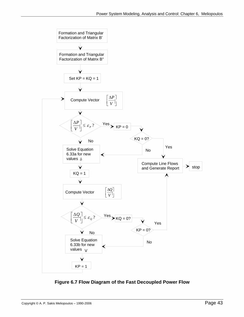
There are several algorithmic possibilities for the solution of the power flow problem with the aid of equations (6.34a) and (6.34b). The most efficient one involves successive solutions of (6.34a) and (6.34b). This algorithm is known as the PQ algorithm because the real power (P) equations are solved first, then the reactive power (Q) equations are solved and the process is repeated again. Both matrix equations (6.34a) and (6.34b) contain a constant matrix. Namely, B' and B''. The solution of either equation is obtained by first computing the symbolic inverse of the matrix (triangular factorization, see Appendix A), then computing the driving vector
[ ∆PV
] or [ ∆QV
] and then by performing a forward and back substitution (see Appendix A)
on the driving vectors. Figure 6.7 illustrates the flow diagram of the PQ algorithm. Note that, in general, different convergence criteria of the real and reactive power flow equations are used, (εp and εq, respectively). It is important to note that the algorithm
terminates whenever ∆PV p< ε and ∆Q
V q< ε . Since the voltage magnitude are near
unity, above conditions are equivalent to: ppp bxf ε<−)(
Copyright © A. P. Sakis Meliopoulos – 1990-2006 Page 41

Power System Modeling, Analysis and Control: Chapter 6, Meliopoulos
qqq bxf ε<−)( In other words the power flow equations are satisfied within εp and εq ; i.e. the algorithm terminates to the exact solution of the power flow equations. The fact that the Jacobian matrix was approximated with a constant matrix does not affect the final solution, assuming that the algorithm converges.
The fast decoupled power flow method is illustrated with two examples.
Page 42 Copyright © A. P. Sakis Meliopoulos – 1990-2006
Power System Modeling, Analysis and Control: Chapter 6, Meliopoulos
Formation and TriangularFactorization of Matrix B'
Formation and TriangularFactorization of Matrix B"
Set KP = KQ = 1
Compute Vector
Yes
KQ = 0?
YesNo
No
Solve Equation6.33a for newvalues
KQ = 1
Compute Vector
Solve Equation6.33b for newvalues
KP = 1
KQ = 0?
Compute Line Flowsand Generate Report Stop
KP = 0
KP = 0?
Yes
No
No
Yes
δ
V
stop
⎥⎦⎤
⎢⎣⎡∆
VP
⎥⎦⎤
⎢⎣⎡∆
VQ
?PVP ε≤⎥⎦
⎤⎢⎣⎡ ∆
?QVQ ε≤⎥⎦
⎤⎢⎣⎡ ∆
Figure 6.7 Flow Diagram of the Fast Decoupled Power Flow
Copyright © A. P. Sakis Meliopoulos – 1990-2006 Page 43

Power System Modeling, Analysis and Control: Chapter 6, Meliopoulos
Example E6.11: Solve the power flow equations of Example E6.1 with the Fast Decoupled Power Flow method. Solution: The algorithmic equations are:
⎥⎦
⎤⎢⎣
⎡ +−= −+
2
2212
12
85.0sin05.5)05.5(
VV δ
δδ υυ
⎥⎦
⎤⎢⎣
⎡ +−−= −+
2
222
212
12
36.0cos05.55)95.4(
VVV
VVδυυ
Starting with δ2 = 0, V2 = 1.0, the first three iterations are 1st iteration = 0 -(5.05)δ2
1 -1(0.85) = -0.1683
= 1.0 - (4.95)V21 -1(0.31) = 0.9373
2nd iteration = -0.1683 - (5.05)δ2
2 -1(0.061) = -0.1804
= 0.9373 - (4.95)V22 -1(0.092) = 0.9187
3th iteration = -0.1804 - (5.05)δ2
3 -1(0.019) = -0.1842
= 0.9187 - (4.95)V23 -1(0.0173) = 0.9152
Above solution should be compared to the solution obtained for the same problem using Gauss method (Example E6.6) and Newton’s method (Example E6.8). Example E6.12: For the electric power system of Figure E6.2, Example E6.2 develop the iterative equations for the fast decoupled load flow and perform two iterations of the method. Solution: From the circuit diagram of the system in Figure E6.3, the matrices B' and B" are obtained by inspection:
Page 44 Copyright © A. P. Sakis Meliopoulos – 1990-2006

Power System Modeling, Analysis and Control: Chapter 6, Meliopoulos
and ⎥⎥⎥
⎦
⎤
⎢⎢⎢
⎣
⎡
−−−
−=
625.25125.130125.13125.229
0919'B ⎥
⎦
⎤⎢⎣
⎡−
−=
275.24125.13125.13397.23
''B
Upon inversion one obtains:
and ⎥⎥⎥
⎦
⎤
⎢⎢⎢
⎣
⎡=−
062575.045981.02178.045981.089772.042524.02178.042524.072774.
]'[ 1B ⎥⎦
⎤⎢⎣
⎡=−
057532.033176.033176.063065.
]''[ 1B
⎥⎥⎥⎥⎥
⎦
⎤
⎢⎢⎢⎢⎢
⎣
⎡
+−+
−−−−−−+
=⎥⎦⎤
⎢⎣⎡∆
νυυυυ
υυυυυ
υυυυ
δδδ
δδδδδδδ
43434
43423
3232
2.2)sin(125.13sin5.12
)sin(125.13)sin(18.97647.1)sin(9sin10
VV
VV
VP
and
⎥⎥⎥
⎦
⎤
⎢⎢⎢
⎣
⎡
+−−−
+−−−=⎥⎦
⎤⎢⎣⎡∆
+++
++++
νυυυυυ
υυυυυυ
δδδ
δδδδ
4
13
143
144
31
41
341
21
35.0)cos(125.13cos5.1295.24
761.22)cos(125.13)cos(18.9
VVV
VV
VQ
The algorithm reads
][]'[ 11
VPB ∆
−= −+ υυ δδ
][]''[ 11
VQBVV ∆
−= −+ υυ
Next two iterations of the method are performed starting from a flat start, that is δ2
0 = δ30 = δ4
0 = 0.0, V30 = V4
0 = 1.0 1st iteration: By direct substitution
⎥⎥⎥
⎦
⎤
⎢⎢⎢
⎣
⎡−=⎥⎦
⎤⎢⎣⎡∆
2.207647.1
VP
and
⎥⎥⎥
⎦
⎤
⎢⎢⎢
⎣
⎡
−−=⎥⎦
⎤⎢⎣⎡∆
−⎥⎥⎥
⎦
⎤
⎢⎢⎢
⎣
⎡= −
0992.0261.
0805.]'[
000
11
VPBδ
Copyright © A. P. Sakis Meliopoulos – 1990-2006 Page 45
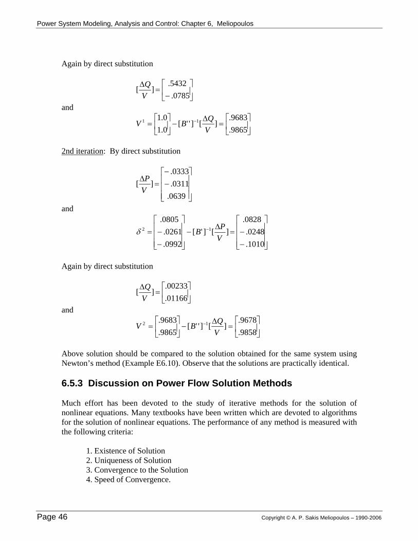
Power System Modeling, Analysis and Control: Chapter 6, Meliopoulos
Again by direct substitution
⎥⎦
⎤⎢⎣
⎡−
=∆
0785.5432.
][VQ
and
⎥⎦
⎤⎢⎣
⎡=
∆−⎥
⎦
⎤⎢⎣
⎡= −
9865.9683.
][]''[0.10.1 11
VQBV
2nd iteration: By direct substitution
⎥⎥⎥
⎦
⎤
⎢⎢⎢
⎣
⎡−−
=∆
0639.0311.0333.
][VP
and
⎥⎥⎥
⎦
⎤
⎢⎢⎢
⎣
⎡
−−=
∆−
⎥⎥⎥
⎦
⎤
⎢⎢⎢
⎣
⎡
−−= −
1010.0248.
0828.][]'[
0992.0261.
0805.12
VPBδ
Again by direct substitution
⎥⎦
⎤⎢⎣
⎡=
∆01166.00233.
][VQ
and
⎥⎦
⎤⎢⎣
⎡=
∆−⎥
⎦
⎤⎢⎣
⎡= −
9858.9678.
][]''[9865.9683. 12
VQBV
Above solution should be compared to the solution obtained for the same system using Newton’s method (Example E6.10). Observe that the solutions are practically identical. 6.5.3 Discussion on Power Flow Solution Methods Much effort has been devoted to the study of iterative methods for the solution of nonlinear equations. Many textbooks have been written which are devoted to algorithms for the solution of nonlinear equations. The performance of any method is measured with the following criteria: 1. Existence of Solution 2. Uniqueness of Solution 3. Convergence to the Solution 4. Speed of Convergence.
Page 46 Copyright © A. P. Sakis Meliopoulos – 1990-2006

Power System Modeling, Analysis and Control: Chapter 6, Meliopoulos
The performance of a method depends on the specific properties of the problem under consideration. In the case of the power flow problem, much theoretical work has been done and much experience has been accumulated over the years. The characteristics of the algorithms as applied to the solution of the power flow problem are very well known. Yet there is no guarantee that given a system the solution can be found (convergence). On the other hand, the practical experience with these methods indicates that nonconvergence of the power flow problem is rather seldom.
6.6 The DC Power Flow Model In several applications it is expedient to seek a quick but approximate solution to the power flow problem. This objective is accomplished with the so-called DC power flow (or DC Network Model) which is presented in this section for completeness. The DC power flow results from a simplification and linearization of the rather complex and nonlinear power flow equations. The simplification results in a model which describes the flow of real power only. The flow of reactive power is ignored. This model has been extensively used in the past and has been useful for planning studies where an approximate evaluation of the real power flow is needed. The basic assumptions utilized in the development of the DC power flow are: a) gkm ≅ 0 (lossless circuits) b) sinδ ≅ δ (phase angle differences are relatively small) c) V≅1.0 pu (all voltages remain constant, near nominal values) Considering the real power equation for a bus k, and applying above assumptions:
∑∑∑∈∈∈
−≅−+=−=)()()(
2 )(kKm
mkmkkKm
mkmkkKm
skmkmkdkgkk VVVVggVPPP αα
Also note that:
)()sin()sin()cos( mkkmmkkmmkkmmkkmkm bbbg δδδδδδδδα −≅−≅−+−= Thus, the real power equation for bus k becomes ∑
∈
−−=)(
)(kKm
mmkkmkk VbVP δδ (6.35)
Define kmmkkm bVV=γ ∑
∈
−=)(kKm
kmkk aγ
Copyright © A. P. Sakis Meliopoulos – 1990-2006 Page 47

Power System Modeling, Analysis and Control: Chapter 6, Meliopoulos
Then equation (6.35) becomes:
(6.36) m
n
mkmkP δγ∑
=
=1
Equation (6.36) implies that the real power flow on a circuit connected between buses k and m, Pkm, is given by: )( mkkmkmP δδγ −−= (6.37) An Equation (6.36) can be written for every bus in the system except the slack bus. For a system of n buses, a total of n-1 equations can be written. In compact matrix form, these equations read: δΓ=P (6.38)
where, and ⎥⎥⎥
⎦
⎤
⎢⎢⎢
⎣
⎡=
nP
PP M
2
⎥⎥⎥
⎦
⎤
⎢⎢⎢
⎣
⎡=
3
2
δ
δδ M
[ ] kmkm γ=Γ Solution of equation (6.38) yields the phase angles. Substitution into equation (6.37) yields the circuit flows. The DC power flow will be illustrated with an example. Example E6.13: Consider the four-bus system of Figure E6.13. The figure illustrates the positive sequence equivalent network of the system. The real power load at bus 4 is 2.0 pu. Write the DC power flow equations for this circuit. Solve the DC power flow and compute the flows in each circuit.
Page 48 Copyright © A. P. Sakis Meliopoulos – 1990-2006

Power System Modeling, Analysis and Control: Chapter 6, Meliopoulos
j0.2
-j10
4
3
21
-j8.0 -j9.0
-j15.0-j12.5
-j0.63-j12.6 j0.60
Figure E6.13. Simplified Four-Bus System, Positive Sequence Equivalent Circuit
Solution: By inspection of the circuit of Figure E6.13 the DC power flow equations are:
, Pd4 = 2.0 ⎥⎥⎥
⎦
⎤
⎢⎢⎢
⎣
⎡
⎥⎥⎥
⎦
⎤
⎢⎢⎢
⎣
⎡
−−−−−−
=⎥⎥⎥
⎦
⎤
⎢⎢⎢
⎣
⎡
− 4
3
2
4 1.406.12156.126.299
1593400
δδδ
dP Solution of above equations yields: δ2 = −0.0515 δ3 = -0.05205 δ4 = -0.08549 Note that δ1= 0.0. The circuit flows are computed and illustrated on Figure E6.13a
Copyright © A. P. Sakis Meliopoulos – 1990-2006 Page 49

Power System Modeling, Analysis and Control: Chapter 6, Meliopoulos
1 2
3
4
.515
.005.416
.5098
.421
1.0686
Figure E6.13a Circuit Flows for Example System of Figure E6.13 (DC Network Model)
6.7 External System Equivalents Interconnections among power systems result in extremely large networks. As an example, the entire eastern United States represents one interconnected system. Network analysis in which the entire network is explicitly represented becomes a computationally difficult task (excessive computational time). Yet the industry is moving towards larger and larger systems. The computational issue and associated long execution times can be addressed in two ways: (a) development of more efficient computational procedures and more sophisticated sparcity methods, and (b) use of equivalencing techniques, where warranted, to reduce the size of the system model. In this section we address the latter approach. Specifically, we discuss methodologies by which the external systems are represented with simplified equivalents. In this context, the external system is any part of the interconnected system that is not vital to the application under consideration. Equivalents reduce the size of the network problem and, therefore, reduce the computational requirements. In the process, some accuracy is sacrificed. The problem of external system equivalents is depicted in Figure 6.8a. The system of interest is interconnected to other systems via tie lines. The other systems may be also interconnected among themselves. For the purpose of defining an equivalent, Tinney, et al [???] suggested that the interconnected system be separated into:
• the internal system or system of interest • the boundary system • the external system, which contains nodes and circuits which are not essential to
the problem.
Page 50 Copyright © A. P. Sakis Meliopoulos – 1990-2006

Power System Modeling, Analysis and Control: Chapter 6, Meliopoulos
The structure (or detailed model) of the internal system must be maintained. The structure of the external system need not be maintained and, therefore, can be represented with an equivalent system connected to the buses of the boundary system. Such an equivalent is represented in Figure 6.8b. The equivalent model of the external system should have the following properties: (a) network solution times for the system of interest, boundary and external equivalent should be much shorter as compared to solution times for the entire network; and (b) the accuracy of the solution must be reasonable. Equivalencing techniques for external power systems have been developed with above criteria. In general, the techniques may be based on the DC Network Model or the AC Network Model. The basis of these techniques is presented next. The computational and accuracy properties of the equivalents are discussed.
Copyright © A. P. Sakis Meliopoulos – 1990-2006 Page 51

Power System Modeling, Analysis and Control: Chapter 6, Meliopoulos
External System, e
Boundary System, b
Internal System, i
Internal System, i
(a)
(b)
Equivalentof Boundaryand
external Systems
Figure 6.8 General Description of External, Boundary and Internal System (a) Actual System
(b) Equivalent System
Page 52 Copyright © A. P. Sakis Meliopoulos – 1990-2006

Power System Modeling, Analysis and Control: Chapter 6, Meliopoulos
6.7.1 Equivalents Based on DC Network Model Formulation Equivalents based on DC network model formulation are adequate in applications where the DC network model is acceptable for the purpose of computing network solutions. Consider an interconnected power system in which an internal, a boundary, and an external system have been identified. The DC power flow equations for the entire system are:
(6.39) ⎥⎥⎥
⎦
⎤
⎢⎢⎢
⎣
⎡=
⎥⎥⎥
⎦
⎤
⎢⎢⎢
⎣
⎡
⎥⎥⎥
⎦
⎤
⎢⎢⎢
⎣
⎡
e
b
i
e
b
i
eeeb
bebbbi
ibii
PPP
AAAAA
AA
δδδ
0
0
where subscript i denotes internal system, subscript b denotes the boundary system and subscript e denotes the external system. Note that the system variables have been partitioned into internal (δi), boundary (δb), and external (δe) system variables. It is assumed that the separation of the system into internal, boundary, and external is such that no connection exists between the external and the internal systems. This selection results in two zero submatrices of equation (6.39) The last matrix equation (of the system 6.39) can be solved for δe, yielding δe = Aee
-1Pe - Aee-1Aebδb
Upon substitution of δe in the remaining equations and rearranging the terms:
(6.40) ⎥⎦
⎤⎢⎣
⎡−
=⎥⎦
⎤⎢⎣
⎡⎥⎦
⎤⎢⎣
⎡− −−
eeebeb
i
b
i
ebeebebbbi
ibii
PAAPP
AAAAAAA
11 δδ
Equation (6.40) suggests that the DC network model matrix of the internal system, the boundary system, and the equivalent of the external system is:
(6.41) ⎥⎦
⎤⎢⎣
⎡−
= −ebeebebbbi
ibii
AAAAAAA
A 11
On the other hand, the DC power flow equations of the internal system and the boundary system (neglecting the existence of the external system) are :
(6.42) ⎥⎦
⎤⎢⎣
⎡=⎥
⎦
⎤⎢⎣
⎡⎥⎦
⎤⎢⎣
⎡
b
i
b
iow
bbbi
ibii
PP
AAAA
δδ
/
with the DC network model matrix being
Copyright © A. P. Sakis Meliopoulos – 1990-2006 Page 53

Power System Modeling, Analysis and Control: Chapter 6, Meliopoulos
(6.43) ⎥⎦
⎤⎢⎣
⎡= ow
bbbi
ibii
AAAA
A /2
where Abb
w/o is the DC network model matrix of the boundary buses if the external system is removed.
Equations (6.40) and (6.42) suggest that the parameters of the external system equivalent are defined with the following equivalent DC network model matrix and power injections: (6.44) ow
bbebeebebbeq AAAAAA /1 −−= −
(6.45) eeebeeq PAAb 1−−= Note the following properties of the above defined equivalent.
• The parameters of the equivalent system depend on power injections in the buses of the external system and the parameters of the circuits of the external system.
• The topology of the external system must be known. • The equivalent representation of the external system is exact in the sense that
solutions for the internal system are identical to those obtained with the entire system.
The equation for Aeq and beq have a physical interpretation. Specifically, the matrix Aeq represents equivalent circuits connected to the boundary buses and the vector beq represents equivalent injections to boundary buses. The procedure will be illustrated with an example. Example E6.14: Consider the electric power system of Figure E6.14a. The external, boundary, and internal systems are defined in the Figure. Compute an equivalent of the external system using DC network model.
1
2
3
4
-j8
-j15
-j12-j80.8 pu
-j10
0.5 puP
D= 2.0
External System
Boundary System
Figure E6.14. Example Four-Bus System Separated into External and
Boundary Systems
Page 54 Copyright © A. P. Sakis Meliopoulos – 1990-2006

Power System Modeling, Analysis and Control: Chapter 6, Meliopoulos
Solution: First the DC power flow equations are written by ordering the buses into internal, boundary and external as follows: Internal: Bus 2 Boundary: Buses 1, and 4 External: Bus 3 The DC Power Flow equations for the entire system are:
⎥⎥⎥
⎦
⎤
⎢⎢⎢
⎣
⎡
−
−=
⎥⎥⎥
⎦
⎤
⎢⎢⎢
⎣
⎡
⎥⎥⎥
⎦
⎤
⎢⎢⎢
⎣
⎡
−−−
−
8.05.00.2
1810010371501523
3
4
2
δδδ
Upon elimination of the external system variables, δ3, the DC power flow equations read
⎥⎦
⎤⎢⎣
⎡−−
=⎥⎦
⎤⎢⎣
⎡⎥⎦
⎤⎢⎣
⎡+−−
444.05.00.2
)444.427(151523
4
2
δδ
Note also that Ybb
w o = 27. Thus, Aeq = 4.444, and beq = -0.444. The above equations correspond to the system of Figure E6.14a. Note that bus 3 (the external system) has been eliminated. In its place an equivalent circuit with admittance b14 = -j4.444 and an equivalent load at bus 4 of 0.444 pu appears.
0.5
-j8 -j12
-j15P
D= 2.0
-j4.444
0.444
1
Figure E6.14a Equivalent System of the Network of Figure E6.14
Copyright © A. P. Sakis Meliopoulos – 1990-2006 Page 55

Power System Modeling, Analysis and Control: Chapter 6, Meliopoulos
6.7.2 Equivalents Based on AC Network Model Formulation This section provides a formulation for the computation of an equivalent representation of the external system which addresses reasonably well the requirements of equivalent models. The formulation assumes complete knowledge of the external system. Again we use Tinney's et al [???] suggestion to separate the system into internal, boundary, and external systems. Using this decomposition, the nodal equations are written as
VYI ~~ = or ⎥⎥⎥
⎦
⎤
⎢⎢⎢
⎣
⎡
⎥⎥⎥
⎦
⎤
⎢⎢⎢
⎣
⎡=
⎥⎥⎥
⎦
⎤
⎢⎢⎢
⎣
⎡
e
b
i
eeeb
bebbbi
ibii
e
b
i
VVV
YYYYY
YY
III
~~~
0
0
~~~
(6.46)
The power flow equations for the entire system are written as *** ~~~~ VYVIVS dd == (6.47) where is the admittance matrix of the entire system Y V
~ is the vector of com , plex voltages at the buses of the entire system
V~d = diag V
~1, V
~2, ..., V
~n,i.e. a diagonal matrix.
Upon separation of the power flow equations into the internal, boundary, and external system equations: *~~
id
ii IVS =
*~~b
dbb IVS =
*~~e
dee IVS =
Where: ...,~,~~
21 iid
i VVdiagV =
...,~,~~21 bb
db VVdiagV =
...,~,~~21 ee
de VVdiagV =
Combining the model equations and the expressions for bus powers, the power flow equations for the three subsystems are obtained. Si = V
~ d [Yii* V~
+ Yib* V~
] i i* b* Sb =
~b
d [Ybi* V~
i* + Ybb* V~
* + Ybe* V~
e*] V b Se = V
~ed [Yeb* V
~b* + Yee* V
~e*]
Page 56 Copyright © A. P. Sakis Meliopoulos – 1990-2006

Power System Modeling, Analysis and Control: Chapter 6, Meliopoulos
From above equations, the external system state variables, V
~e, are to be eliminated. To
simplify the procedure, assume that the external system contains only one bus. (No loss of generality occurs since the procedure to be described can be applied to each external bus sequentially.) In this case, Se, V
~ed, V
~e, and Yee are scalars. Now the last equation
becomes: 0~)~( **2* =−+ eebebeee SVVYVY Note that above equation is quadratic with respect to the voltage phasor at the external system bus. Direct elimination of the voltage phasor at the external system bus is not always possible because of the complexity of the solution. Specifically, a direct solution of above equation for the magnitude of the voltage, Ve, yields:
ee
eeej
bebj
bebe Y
SYeVYeVYV
ee
24)~(~ *2 +±−
=δδ
You can verify above solution by simply substituting into the quadratic equation. Note that above solution is rather complex with respect to the voltage phasors at the boundary buses. In addition, the solution is in terms of the phase angle of the voltage at the external bus (this is not a major drawback, since we can assume that the phases may be measured with respect to the external system bus and therefore this phase will be zero). Substitution of above solution into the first two equations will yield rather complex equations in terms of the boundary bus voltages. A simpler solution can be obtained by introducing reasonable approximations. For example, consider the following expression:
2
*
e
e
VS
This expression represents the apparent admittance of the electric load at the external bus. This expression is rather insensitive to the voltage V
~e. Consider, for example, a constant
impedance load. In this case, this expression is is exactly a constant. Let’s denote this ratio with the variable: . Upon substitution of the power variable Se into the last power flow equation, yields:
eY
[ ]****2* ~~~
eeebebeee VYVYVVY += Assuming that the quantity Ye can be treated as a constant in the equivalent representation, the last equation is solved for V
~e yielding:
bebeeee VYYYV ~)(~ 1−−−= (6.48)
Copyright © A. P. Sakis Meliopoulos – 1990-2006 Page 57

Power System Modeling, Analysis and Control: Chapter 6, Meliopoulos
where (6.49) 2* / eee VSY = Upon substitution of V
~e to the other two equations:
Si = V
~id [Yii* V
~i* + Yib* V
~b* ]
Sb = V
~b
d [Ybi* V~
i* + (Ybb* - Ybe*(Yee* - Ye*)-1Yeb*)V~
b ] On the other hand the power flow equations for the internal and boundary systems neglecting the external system will be Si = V
~id [Yii* V
~i* + Yib* V
~b* ]
Sb = V
~b
d [Ybi* V~
i* + Ybbw/o*V
~b
* ]
where Ybb
w/o is the admittance matrix at the boundary buses neglecting the presence of the external system.
By comparison of above equations, the equivalent of the external system has the following admittance matrix: Yeq = Ybb - Ybe (Yee - Ye)-1 Yeb - Ybb
w/o (6.50) Where: Ybb
w/o is the admittance matrix at the boundary buses when the external system is removed.
The equivalent of the external system is given in terms of the quantity Ye which depends on the power injection at the external bus. It is expedient to discuss this quantity. First, whenever the external bus has no power injection (Ye = 0) or when electric load is connected to the buses which can be represented as a constant impedance (Ye = constant), the derived equivalent is an exact equivalent. This means that network solutions using the equivalent or the entire system will provide identical results for the internal system. In any other case, Ye is not a constant. In these cases, appropriate load models or generation models must be utilized to obtain reasonable average values for Ye. This problem, however, is beyond the scope of this text. As in the case of the DC Network model, the equivalent admittance Yeq has a physical meaning. The computation of an equivalent will be demonstrated with an example.
Page 58 Copyright © A. P. Sakis Meliopoulos – 1990-2006
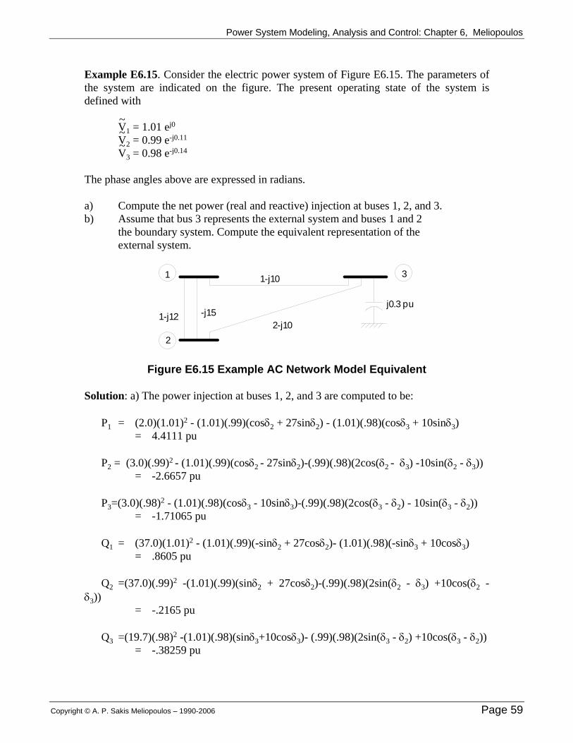
Power System Modeling, Analysis and Control: Chapter 6, Meliopoulos
Example E6.15. Consider the electric power system of Figure E6.15. The parameters of the system are indicated on the figure. The present operating state of the system is defined with V
~1 = 1.01 ej0
V~
2 = 0.99 e-j0.11 V
~3 = 0.98 e-j0.14
The phase angles above are expressed in radians. a) Compute the net power (real and reactive) injection at buses 1, 2, and 3. b) Assume that bus 3 represents the external system and buses 1 and 2 the boundary system. Compute the equivalent representation of the external system.
1
2
31-j10
-j151-j122-j10
j0.3 pu
Figure E6.15 Example AC Network Model Equivalent Solution: a) The power injection at buses 1, 2, and 3 are computed to be: P1 = (2.0)(1.01)2 - (1.01)(.99)(cosδ2 + 27sinδ2) - (1.01)(.98)(cosδ3 + 10sinδ3) = 4.4111 pu P2 = (3.0)(.99)2 - (1.01)(.99)(cosδ2 - 27sinδ2)-(.99)(.98)(2cos(δ2 - δ3) -10sin(δ2 - δ3)) = -2.6657 pu P3=(3.0)(.98)2 - (1.01)(.98)(cosδ3 - 10sinδ3)-(.99)(.98)(2cos(δ3 - δ2) - 10sin(δ3 - δ2)) = -1.71065 pu Q1 = (37.0)(1.01)2 - (1.01)(.99)(-sinδ2 + 27cosδ2)- (1.01)(.98)(-sinδ3 + 10cosδ3) = .8605 pu Q2 =(37.0)(.99)2 -(1.01)(.99)(sinδ2 + 27cosδ2)-(.99)(.98)(2sin(δ2 - δ3) +10cos(δ2 - δ3)) = -.2165 pu Q3 =(19.7)(.98)2 -(1.01)(.98)(sinδ3+10cosδ3)- (.99)(.98)(2sin(δ3 - δ2) +10cos(δ3 - δ2)) = -.38259 pu
Copyright © A. P. Sakis Meliopoulos – 1990-2006 Page 59

Power System Modeling, Analysis and Control: Chapter 6, Meliopoulos
b) The equivalent admittance matrix due to elimination of bus 3 is:
Yeq = Ybb - Ybe(Yee + Ye)-1Yeb - Ybbw/o
where: Yee = (3 - j19.7) Yeb = Ybe
T = [-1 + j10 -2 + j10]
⎥⎦
⎤⎢⎣
⎡−
−=−
10200101/
jj
YY owbbbb
39826.07812.1)98(. 2
*3 j
SYe +−==
upon evaluation of above expression:
⎥⎦
⎤⎢⎣
⎡−+−+−−
=0317.51918.19505.43148.9505.43148.1135.51678.1
jjjj
Yeq
The equivalent is illustrated in Figure E6.15a.
(b)
1
2
-j.163.853
.877 -j.0812
-j4.9505.3148
1-j12
-j15
Figure E6.15a Equivalent System of the AC Network Model of Figure E6.15
6.7.3 Discussion on Equivalents It is necessary to represent external power systems with reduced size equivalents. This representation is necessary for a variety of applications. Computation of equivalents encounters difficulties because of the nonlinear characteristics of the electric load and generation in the external system. A method has been presented which computes an approximate equivalent circuit of the external system. The method requires knowledge of
Page 60 Copyright © A. P. Sakis Meliopoulos – 1990-2006

Power System Modeling, Analysis and Control: Chapter 6, Meliopoulos
the external system. In real time applications, since the external system changes continuously, the equivalent must be frequently updated.
6.8 Quadratized Power Flow Model Because of the importancve of the power flow model as one of the basic analysis tools in the operation and planning of power systems, many attempts have been made to improve the efficiency of power flow solutions. Thes attempts range from different formulations of the power flow problem to advanced sparcity methods and shortcuts for repeat solutions. Sparcity methods are discussed in ASppendix A. Advanced methods for repeat solutions are discussed in the context of power system securioty in Chapter 11. In this section, we discuss attempts to formulate the power flow problem in a way that will improve the efficiency of the solution methods. In this context, it was observed in the early seventies that expressing the bus voltage phasors in Cartesian coordinates, the resulting power flow problem is less complex since trigonometric functions are absent. For whatever reason, the Cartesian coordinate formulation did not go very far. Recently, a similar idea has surfaced. The idea is to “quadratize” the power flow equations, i.e. to express the power flow equations as a set of equations with order no greater than two. It turns out this can be achieved very easily with the introduction of additional state variables as needed. The advantage of this formulation is that the resulting power flow equations are either linear or quadratic. Application of Newton’s method to these equations yields the solution very quickly since Newtron’s method is ideally suitable to quadratic equations. The formulation of the power flow problem as a set of linear and quadratic equations is presented next. Consider a bus of an electric power system as it is illustrated in Figure 6.9. The Figure shows a generator, a constant impedance load, a constant power load, an induction motor load, and switched shunt capacitor/reactors are connected to the bus together with a transformer and a circuit (transmission line) to other buses. Each component of the power system illustrated in Figure 6.9 can be modeled with a set of linear and quadratic equations. As an example, the form of the models for a generator, a circuit and a constant power load model is described next.
BUS30
+S
EQ
S
G
MZ
Copyright © A. P. Sakis Meliopoulos – 1990-2006 Page 61

Power System Modeling, Analysis and Control: Chapter 6, Meliopoulos
Figure 6.9: Symbolic Representation of a General Power System Bus –
Positive Sequence Network Generator Model: Figure 6.10 illustrates the simplified equivalent circuit model of a single axis generator model.
~Ek
~
Vk~jb
Bus kIk
~
Figure 6.10
The electric current of the generator, in the direction from the bus into the generator, is given by the equation: ( )kkk EVjbI ~~~ −= (6.51) where jb is the generator admittance. Note here we use the single axis model of the generator. The procedure can be applied to the two axes model of the generator as well. This is omitted to avoid the complexity of the two axes model equations. There are three control modes for the synchronous generator, i.e., a) Slack mode, b) PQ mode, and c) PV mode. The model of each one of these cases is described next. Slack mode: In the slack mode, the synchronous generator is controlled to maintain the specified voltage magnitude and zero phase. For the slack mode, we have the following equations. ( )kkk EVjbI ~~~ −= (6.52a) (6.52b) kiV=0.0 (6.52c) 2
,220.0 specifiedkkikr VVV −+=
Note that equation (6.52a) forces the phase of the generator terminal voltage to be zero. Equation (6.52c) forces the magnitude of the generator terminal voltage to be equal to the specified.
Page 62 Copyright © A. P. Sakis Meliopoulos – 1990-2006

Power System Modeling, Analysis and Control: Chapter 6, Meliopoulos
PQ mode: In the PQ mode, the synchronous generator is controlled to maintain the specified real and reactive power. For the PQ mode, we have the following equation. ( )kkk EVjbI ~~~ −= (6.53a) (6.53b) specifiedkspecifiedkkkk jQPEVjbjbV ,,
*2 ~~0.0 +++−=
Note that equation (6.53b) imposes the requirement that the complex power delivered by the generator equals the specified complex power. PV mode: In the PV mode, the synchronous generator is controlled to maintain the specified real power and voltage magnitude. For the PV mode, we have the following equations. ( )kkk EVjbI ~~~ −= (6.54a)
specifiedkkkk PEVjbjbV ,*2 ~~Re0.0 ++−= (6.54b)
(6.54c) 2,
220.0 specifiedkkikr VVV −+= Note that equation (6.54b) imposes the requirement that the real power delivered by the generator is equal to the specified real power. Equation (6.54c) imposes the requirement that the magnitude of the terminal voltage equals the specified voltage. In each of the above cases we have an equation that describes the current at the terminal of the generator as a function of state variables and some additional equations expressing the control functions of the generator. All equations are linear or quadratic in terms of the state variables. Circuit Branch Model: Figure 6.11 illustrates the model of a circuit represented with its pi-equivalent circuit.
BUS K BUS m
Ikm~ Imk
~ykm~
yskm~ ysmk
~
Figure 6.11
The circuit model is represented with the following equations:
Copyright © A. P. Sakis Meliopoulos – 1990-2006 Page 63

Power System Modeling, Analysis and Control: Chapter 6, Meliopoulos
( ) mkmkskmkmk VyVyyI ~~~~~~−+= (6.55a)
( msmkkmkkmm VyyVyI )~~~~~~++−= (6.55b)
Where:
kmy~ is the circuit series admittance skmy~ is the k side shunt admittance smky~ is the m side shunt admittance kV~ is the voltage phasor at bus k. mV~ is the voltage phasor at bus m.
Note that these equations are linear with respect to the state variables.
a) Constant Power Load Model: Figure 6.12 shows a constant power load that is connected to bus k. The constant power load is defined with the total complex power, dkdkdk jQPS += , that is assumed to be constant, i.e. independent of the voltage magnitude at the bus.
Idk~
BUS K
Pdk+jQdk
a. Figure 6.12. Constant Power Load at Bus k Define the nominal admittance of the load to be:
( ) kdnkdndkdknk
kdn jbgjQPV
Y ,,2,1
+=−= (6.56)
where: Vnk is the nominal voltage at bus k. Then the constant power load model can be expressed with the following set of equations. kkdnkkdndk VYuVYI ~~~
,1, += (6.57a)
Page 64 Copyright © A. P. Sakis Meliopoulos – 1990-2006

Power System Modeling, Analysis and Control: Chapter 6, Meliopoulos
(6.57b) dkkdnkdn Puugug −+= 21,2,0
(6.57c) 220 kVu −=
Above equations force that the complex power absorbed by the load is equal to the specified load and constant. The reader is encouraged to prove this as follows. Note that the complex power absorbed by this load is: dkk IVS ~~= Upon substitution of the current with equation (6.57a) and elimination of the variable u1 with the aid of equations (6.57b) and (6.57c), the complex power S becomes identical to the specified power of the load. The three examples above show that each component of the system can be represented with an appropriate set of linear or quadratic equations. Upon expressing the voltage and current phasors with their Cartesian coordinates, (i.e. ir III +=~ , and ir VVV +=~ ) and separating each complex equation into two real equations, the following general form is obtained for any power system component:
(6.58) kk
realeqTk
kkrealeq
Tk
k
ki
kr
kki
kr
realeqrealeqbxfx
xfx
yVV
yII
__ 2_
1_
0−
⎥⎥⎥⎥⎥
⎦
⎤
⎢⎢⎢⎢⎢
⎣
⎡
+⎥⎥⎥
⎦
⎤
⎢⎢⎢
⎣
⎡
=⎥⎥⎥
⎦
⎤
⎢⎢⎢
⎣
⎡
M
where: ⎥⎥⎥
⎦
⎤
⎢⎢⎢
⎣
⎡
=k
ki
kr
k
yVV
x
and , , and are matrices with appropriate dimensions. krealeqy _
krealeqb _
krealeqf _
We have discussed the general quadratic model of three components of an electric power system, namely, generator, line and constant power load. It is emphasized that this procedure can be applied to any other component, i.e. transformer, variable tap transformer, two axes generator model, etc. The end result will always be a model in the form of equation (6.58). Solution Method: The network solution is obtained with application of Newton’s method to a quadratized form of the network equations. The quadratized network equations are generated as follows. Consider the general form of equations for any model of the system (linear or nonlinear), i.e. equation (6.58). Note that this form includes two sets of equations, which are named external equations and internal equations respectively. The electric currents at the terminals of the component appear only in the
Copyright © A. P. Sakis Meliopoulos – 1990-2006 Page 65

Power System Modeling, Analysis and Control: Chapter 6, Meliopoulos
external equations. Similarly, the device states consist of two variable sets: external states (i.e. bus voltages k
ik
rk jVVV +=~ ) and internal state variables (if any). The set
of equations (6.58) is consistent in the sense that the number of external states and the number of internal states equals the number of external and internal equations respectively.
ky
The entire network equations are obtained by application of the connectivity constraints among the system component, i.e. Kirchoff’s current law at each system bus. Specifically, Kirchoff’s current law applied to all buses of the system yields: 0IA
k
kk =∑ ~
where k
ikr
k jIII +=~ is device k bus current injections, and Ak is a component incidence matrix with:
⎭⎬⎫
⎩⎨⎧
=otherwise
ibustoconnectediskdeviceofjbusifAk
ij ,0,1
To above equation all the internal equations from all devices should be added, yielding the following set of equations: 0IA
k
kk =∑ ~ (6.59a)
[internal equations of all devices] (6.59b) Let ir jVVV +=~ be the vector of all bus voltage phasors. Then, the following relationship holds: VTkk AV
~)(~ = (6.60) where kV~ is device k bus voltages. Equations (6.59a) can be separated into two sets of real equations by expressing the voltages and currents with their Cartesian coordionates. Then the device currents can be eliminated with the use of equations (6.58). This procedure will yield a set of equations in terms of the voltage variables and the internal device state variables. If all the state variables are represented with the vector x, then the equations can be written in the following form:
Page 66 Copyright © A. P. Sakis Meliopoulos – 1990-2006

Power System Modeling, Analysis and Control: Chapter 6, Meliopoulos
(6.61) 0)( 2
1
=−⎥⎥⎥
⎦
⎤
⎢⎢⎢
⎣
⎡
+= realT
T
real Bxfxxfx
xYxGM
where x is the vector of all the state variables and are matrices with appropriate dimensions. The simultaneous solution of these equations is obtained via Newton’s method described next.
realreal BfY ,,
Equation (6.61) is solved using Newton’s method. Specifically, the solution is given by the following algorithm:
(6.62)
⎪⎪⎭
⎪⎪⎬
⎫
⎪⎪⎩
⎪⎪⎨
⎧
−
⎥⎥⎥⎥
⎦
⎤
⎢⎢⎢⎢
⎣
⎡
+−= −+real
T
T
realG Bxfx
xfx
xYJxxM
νν
νν
ννν2
1
11
where is the iteration step number; is the Jacobian matrix of equation (6.61). In particular, the Jacobian matrix takes the following form:
ν GJ
(6.63)
⎥⎥⎥⎥
⎦
⎤
⎢⎢⎢⎢
⎣
⎡
+
+
+=M
)(
)(
22
11
TT
TT
realG ffx
ffx
YJ ν
ν
It is important to note that Newton’s method is ideally suited for solution of quadratic equations. The quadratic power flow is demonstrated with an example. Example E6.16: Consider the power system of Figure E6.16. The generator controls the voltage magnitude at bus 1 to the value of 1.0 pu. Assume that the electric load at bus 2 is Sd2 = 0.85+j0.36 pu. Formulate the Newton-Raphson power flow problem as well as the quadratized power flow problem. Solve both problems starting from flat start, i.e. the voltage at bus 2 equal to 1.0 pu. Record the mismatch at each iteration and tabulate the results.
Copyright © A. P. Sakis Meliopoulos – 1990-2006 Page 67

Power System Modeling, Analysis and Control: Chapter 6, Meliopoulos
1 2-j10
Sd2
2~V
001 0.1~ jeV =
Figure E6.16 A Simplified Two-Bus Example Power System Solution: a) The Newton-Raphon power flow problem for this system is defined with the following equations: 0.085.0sin0.10)( 221 =+= δVxg 0.036.0cos0.100.10)( 22
222 =+−= δVVxg
The iterative solution algorithm is: )()(11 νννν xgxJxx g
−+ −= where:
, , ⎥⎦
⎤⎢⎣
⎡=
2
2
Vx
δ⎥⎦
⎤⎢⎣
⎡=
)()(
)(2
1ν
νν
xgxg
xg ⎥⎦
⎤⎢⎣
⎡−
=2222
222
cos0.100.20sin0.10sin0.10cos0.10
)(δδ
δδVV
VxJ g
The first four iteration of the algorithm yield: The quadratized power flow problem for this system is defined with the following equations: 0.0~)36.085.0)(1()0.1~(0.10 212 =−++−− VjuVj 0.085.085.085.0 212 =−+ uuu 0.02
22 =−Vu Note that the first equation is complex while the second and thord are real. Upon expressing the complex voltage for bus 2 with its Cartesian coordinates and conversion of the complex equation into two real equations yields: 0.00.685.036.085.036.6)( 1212221 =++−+−= uVuVVVyG irir
0.036.085.036.685.0)( 1212222 =+++= uVuVVVyG irir 0.085.085.085.0)( 2123 =−+= uuuyG
Page 68 Copyright © A. P. Sakis Meliopoulos – 1990-2006

Power System Modeling, Analysis and Control: Chapter 6, Meliopoulos
0.0)( 22
2224 =−−= ir VVuyG
Note that the above equations are quadratic and include four unknowns. The iterative solution algorithm is: )()(11 νννν yGyJyy G
−+ −= where:
, ,
⎥⎥⎥⎥
⎦
⎤
⎢⎢⎢⎢
⎣
⎡
=
2
1
2
2
uuVV
y i
r
⎥⎥⎥⎥
⎦
⎤
⎢⎢⎢⎢
⎣
⎡
=
)()()()(
)(
4
3
2
1
yGyGyGyG
yG ν
⎥⎥⎥⎥
⎦
⎤
⎢⎢⎢⎢
⎣
⎡
−−+
++++−+−−
=
0.102285.085.085.000
036.085.036.036.685.085.0085.036.085.085.036.036.6
)(
22
12
2211
2211
ir
ir
ir
G
VVuu
VVuuVVuu
yJ
The iterations for both methods start from the same initial guess: 0
2 0.1~ jeV = . The first three iterations of the algorithm are summarized in Table E6.16. To minimize the data, the table reports the solution at each iteration as well as the following norm:
∑=i
i xgN
g )(1 2
Newton-Rapston Quadratized Power Flow
Iteration V g V g 0 000.1 je 0.6525 000.1 je 0.4615 1 0870.4964.0 je− 0.4049 x 10⁻¹ 0129.595894.0 je− 0.7367 x 10⁻²
2 0086.595854.0 je− 0.2879 x 10⁻³ 0088.595850.0 je− 0.5816 x 10⁻⁵
3 0088.595850.0 je− 0.15 x 10⁻⁷ 0088.595850.0 je− 0.7997 x 10⁻¹¹
It is important to observe in this example that the convergence characteristics of the quadratized power flow are superior to those of the Newto-Raphson method. Specifically, the norm of the mismatches of the quadratized power flow is consistently lower than that of the Newton-Raphson method. For example, at the second iterations, the norm of mismatches of the quadratized power flow is two orders of magnitude lower than that of the Newton-Raphson.
Copyright © A. P. Sakis Meliopoulos – 1990-2006 Page 69

Power System Modeling, Analysis and Control: Chapter 6, Meliopoulos
The quadratized power flow formulation appears to be more complicated than the usual formulation in terms of the polar form of the voltages. However, the advantages of the quadratizerd power flow formulation is the improved convergence characteristics that leads to an overall algorithm that is more efficient than the Newton-Raphson formulation. This property carries to large scale systems.
6.9 Summary and Discussion Network analysis procedures under steady state balanced conditions have been presented. The formulation and solution methods of the power flow problem are the cornerstone of network analysis for power systems. Two distinct formulations have been presented: (l) one using the DC network model and (2) another using the AC network model. The DC network model is a linear model, while the AC network model is a nonlinear model. The solution of the DC power flow is obtained directly. The solution of the AC power flow requires iterative algorithms. Three such algorithms have been presented: (l) the Gauss/Seidel, (2) the Newton/Raphson, and (3) the Fast Decoupled Power Flow. Sparsity techniques are essential in these algorithms and presented in Appendix A. The important problem of external system equivalents has been presented. Finally, a new formulation of the power flow problem has been discussed. This formulation results in a set of linear/quadratic equations. Newton’s method is ideally suited for the solution of this problem resu;lting in superior convergence characteristics.
Page 70 Copyright © A. P. Sakis Meliopoulos – 1990-2006

Power System Modeling, Analysis and Control: Chapter 6, Meliopoulos
6.10 Problems Problem P6.1: Consider the simplified three phase electric power system of Figure P6.1. All parameters and data are marked on the Figure. The three phase transformer rating is 30 MVA, 15 kV: 15 kV with Z = j0.10 pu. a) Draw the per phase equivalent circuit (positive sequence) of the system. Mark all
known data on the drawing. b) Draw the per phase equivalent circuit of the system in per unit. Mark all known data
in per unit. Use the following bases (all phase quantities): Sb = 33.333 MVA, Vb = 6.9282 kV.
c) Write the power flow equations for the system in (b). Use the minimum number of equations and unknowns which define the power flow problem.
Unit G1 Unit G2
j10 Ω
j10 Ω
j10 Ω
j12 Ω
j12 Ω
j12 Ω
+E2
E1
+
E1
E2= 7.25 ej0 = 7.35 e δj
kVkV
150+j20Ω each leg
Figure P6.1 Problem P6.2: Consider the simplified three bus electric power system of Figure P6.2. The transmission line admittance is pujys 0.1012 −= and the regulating transformer series admittance is and its turns ratio t is automatically adjusted so that . The electric load at bus 3 is
pujys 5.1223 −=puV 0.13 = pujSd 5.00.23 += . For this system, the
state of the system is defined with the variables tandV ,,, 322 δδ . a) Write a set of equations which involves only the state variables. b) Develop the Newton algorithm for the solution of the state variables. c) Perform two iterations of the algorithm. What is the required transformer tap ratio?
Copyright © A. P. Sakis Meliopoulos – 1990-2006 Page 71

Power System Modeling, Analysis and Control: Chapter 6, Meliopoulos
yS12
V1
~
yS23
V2
~V3
~
Sd31:t
G1
Figure P6.2
Problem P6.3: Use the Newton method to solve the following set of equations: 2x1
2 + 3x2 - 2 = 0 2x1 + 2x1x2 - 1 = 0 Problem P6.4: Consider the simplified two bus system of Figure P6.4. All the parameters are indicated in the figure. a) Write the iterative equations for solving the power flow problem using the Gauss-
Seidel method. b) Perform five iterations of the algorithm in (a) above. c) Write the iterative equations for solving the power flow problem using the Newton-
Raphson method. d) Perform two iterations of the algorithm in (c) above. e) Write the iterative equations for solving the power flow problem using the fast
decoupled power flow. f) Perform two iterations of the algorithm in (e) above.
S
1 2-j8 pu
= 2.5 + j1.2 pu1.0ej0
G1
1V =
V eV =δj
22
2
Figure P6.4 Problem P6.5: Consider the three bus electric power system of Figure P6.5. Bus 1 is the slack bus, bus 2 is a PV bus, and bus 3 is a PQ bus. Other information is included in the Figure. Write explicitly the iterative equations for the solution of the above load flow problem using the fast decoupled power flow. In your equations, only the state variables must appear. In other words, numerical values must be substituted for all other parameters. Perform two iterations of the algorithm.
Page 72 Copyright © A. P. Sakis Meliopoulos – 1990-2006

Power System Modeling, Analysis and Control: Chapter 6, Meliopoulos
j0.25
SD3 = 2.0 + j0.5 pu
-j10
-j8-j12
12
3
V2 = 0.98 ejδ2
Pg2 = 1.0
V1 = 1.0 ej0
V3 = V3 ejδ3
~
~~
Figure P6.5 Solution: The three power flow equations are:
( )3232 sin84.7sin8.90.1 δδδ −+= V ( )23333 sin84.7sin0.120.2 δδδ −+=− VV
( )233332
3 cos84.7cos0.1275.195.0 δδδ −−−=− VVV The fast decoupled power flow algorithm is:
( )( )
⎥⎥⎥
⎦
⎤
⎢⎢⎢
⎣
⎡
+−+
−−+
⎥⎦
⎤⎢⎣
⎡−
−−⎥
⎦
⎤⎢⎣
⎡=⎥
⎦
⎤⎢⎣
⎡−+
νννν
νννννν
δδδ
δδδ
δδ
δδ
3233
32321
3
21
3
2 0.2sin8sin12
02041.1sin8sin10
0.200.80.80.18
V
V
[ ] ( ) ⎥⎦
⎤⎢⎣
⎡+−−−−= +++−+
ννννννν δδδ
3
12
13
133
13
13
5.0cos84.7cos1275.195.19V
VVV
Two iterations of the algorithm, starting from flat strat yield:
Copyright © A. P. Sakis Meliopoulos – 1990-2006 Page 73

Power System Modeling, Analysis and Control: Chapter 6, Meliopoulos
Problem P6.6: Consider the three bus electric power system of Figure P6.6. Buses 1 and 2 are equipped with generating units which control the voltage at these buses at 1.02 and 1.01 p.u., respectively. At bus 3 there is a synchronous condenser (SC) (a synchronous condenser is a generator of reactive power for the purpose of controlling the voltage). The voltage magnitude at bus 3 is maintained at 1.0 p.u. by the control action of the synchronous condenser. All other specified quantities are indicated in the figure. The indicated circuit parameters are admittances (in pu). a) Characterize the system buses as slack, PV, and or PQ. b) Write the power flow equations (minimum set of equations). c) Write the iterative equations for the solution of the power flow problem using the
Newton-Raphson method. d) Perform two iterations of the method in (c) above. e) Compute the reactive power output of the synchronous condenser. f) Write the iterative equations for the solution of the power flow problem using the
Fast Decoupled Power Flow method. g) Perform two iterations of the algorithm in (f). h) Compare the solutions from (d) and (g).
SL2 = 0.8 + j0.4 pu
|V1| = 1.02
1 2
3
SL3 = 2.0 + j0.5 pu|V3| = 1.0
Pg3 = 0.0S.C.
-j12-j8
-j10
Pg2 = 1.5 pu
|V2| = 1.01~
~
~
Figure P6.6 Solution: (a) Bus 1: Slack, Bus 2: PV and Bus 3: PV (b) The state variables will be: 32 δδ and . The power flow equations are:
Page 74 Copyright © A. P. Sakis Meliopoulos – 1990-2006

Power System Modeling, Analysis and Control: Chapter 6, Meliopoulos
Bus 2: ( ) ( )322 sin12.12sin302.108.05.1 δδδ −+=− Bus 3: ( ) ( )233 sin12.12sin16.80.2 δδδ −+=− (c) The algorithm is:
( ) ( ) ( )( ) ( ) ( )
( ) ( )( ) ( ) ⎥
⎦
⎤⎢⎣
⎡+−+
−−+⎥⎦
⎤⎢⎣
⎡−+−−
−−−+
−⎥⎦
⎤⎢⎣
⎡=⎥
⎦
⎤⎢⎣
⎡
−
+
0.2sin12.12sin16.87.0sin12.12sin302.10
cos12.12cos16.8cos12.12cos12.12cos12.12cos302.10
233
3221
23323
32322
3
21
3
2
δδδδδδ
δδδδδδδδδδ
δδ
δδ νν
(d) Iteration 1: (starting from zero)
⎥⎦
⎤⎢⎣
⎡−−
=⎥⎦
⎤⎢⎣
⎡11810.003259.01
3
2
δδ
Iteration 2:
⎥⎦
⎤⎢⎣
⎡−−
=⎥⎦
⎤⎢⎣
⎡11833.003269.02
3
2
δδ
(e) The reactive power output of the synchronous condenser is:
( ) ( ) 3214.0cos16.8cos12.120.205.0 323 =−−−+= δδδSCQ (f)
( ) ( )( ) ( ) ⎥
⎦
⎤⎢⎣
⎡+−+
−−+⎥⎦
⎤⎢⎣
⎡−
−−⎥
⎦
⎤⎢⎣
⎡=⎥
⎦
⎤⎢⎣
⎡−+
0.2sin12.12sin16.86931.0sin0.12sin2.10
0.200.120.120.22
233
3221
3
21
3
2
δδδδδδ
δδ
δδ νν
(g) Iteration 1: (starting from zero)
⎥⎦
⎤⎢⎣
⎡−−
=⎥⎦
⎤⎢⎣
⎡12054.003426.01
3
2
δδ
Iteration 2:
⎥⎦
⎤⎢⎣
⎡−−
=⎥⎦
⎤⎢⎣
⎡11829.003265.02
3
2
δδ
(h) Final result almost identical. If more iterations will be identical.
Copyright © A. P. Sakis Meliopoulos – 1990-2006 Page 75

Power System Modeling, Analysis and Control: Chapter 6, Meliopoulos
Problem 6.7: A simplified power system, illustrated in Figure P6.7, consists of an off-nominal tap transformer, a capacitor bank, and two buses. When the capacitor switch is open, the state of the system is: , 0
2 10−=δ puV 89.02 = a) Verify that above values satisfy the power flow equations. b) Assume that the switch closes. Compute the new voltage at bus 2 using the fast
decoupled power flow method. Perform two iterations of the method.
G1
1 : 0.95
V1 = 1.0 e j0~
Sd2=0.734+j0.203 pu
Capacitor BankAdmittance
y = j1.0
TransformerLeakage Admittance
y = -j5.0
1V2 = V2 e
~ jδ2
2
Figure P6.7 Solution: (a) The power flow equations are:
734.0sin75.4 22 −=δV 203.0cos75.40.5 22
22 −=− δVV
Above equations are satisfied at the provided values for the magnitude and phase of the voltage. (b) When the switch closes, the power flow equations will be:
734.0sin75.4 22 −=δV 203.0cos75.40.4 22
22 −=− δVV
The fast decoupled power flow algorithm is:
( ) ⎥⎦
⎤⎢⎣
⎡ +−= −+
ννν δ
δδ2
2212
12
734.0sin75.475.4
VV
Page 76 Copyright © A. P. Sakis Meliopoulos – 1990-2006

Power System Modeling, Analysis and Control: Chapter 6, Meliopoulos
( ) ⎥⎦
⎤⎢⎣
⎡ +−−= −+
ννν δ
2
222
212
12
203.0cos75.40.425.3
VVV
VV
Three iterations of the algorithm (starting from the provided solution) yield:
⎥⎦
⎤⎢⎣
⎡−=⎥
⎦
⎤⎢⎣
⎡134.11745.01
2
2
Vδ
⎥⎦
⎤⎢⎣
⎡−=⎥
⎦
⎤⎢⎣
⎡132.11321.02
2
2
Vδ
⎥⎦
⎤⎢⎣
⎡−=⎥
⎦
⎤⎢⎣
⎡131.11375.03
2
2
Vδ
Problem P6.8: An electric power system consists of a transmission line and a transformer as it is illustrated in Figure P6.8. The generator G1 controls the voltage magnitude at bus 1 to 1.0 pu. The total electric load at bus 3 is 1.0+j0.4 pu. The transformer tap is set to the value 1.05 pu as it is indicated in the figure. a) Write the power flow equations for this system. b) Solve the power flow equations using Newton’s method. c) Solve the power flow equations using the fast decoupled power flow method. All relevant values are given in the Figure.
Z=j0.1 pu
G1
1
1:tZ=j0.12 put =1.05
2 3
Figure P6.8
Problem P6.9: Consider the simplified power system of Figure P6.9. It has been decided to eliminate node 3 of the system. Thus node 3 is the external system and therefore buses 1 and 2 will be the boundary buses. The voltage magnitude at bus 3 is 0.98 p.u. Compute the equivalent network representing the eliminated external system.
Copyright © A. P. Sakis Meliopoulos – 1990-2006 Page 77

Power System Modeling, Analysis and Control: Chapter 6, Meliopoulos
SYSTEM OFINTEREST
Sd3= 2.3+j0.8
-j12.5
j0.08 j0.08
y = 1-j12
1
2
3
Figure P6.9 Problem P6.10: Two wye-wye connected three phase transformers are connected in parallel supplying an electric load equal to 200 MW + j 85 MVARs. The tap setting and the leakage admittance of the transformers on a 100 MVA, 230 kV basis are given in Figure P6.10. The generator maintains the voltage magnitude at bus 1 equal to 1.0 pu. a) Compute and graph the pi equivalent circuit of the two parallel transformers. b) Compute the voltage magnitude and phase at the load using the Newton-Raphson
method. Two iterations will suffice. c) Compute the voltage magnitude and phase at the load using the fast decoupled load
flow. Two iterations will suffice. d) Compute the complex power flow in each of the two transformers.
G
1 : 1
1 : 1.022.0 + j0.85 pu
y = -j10 puboth transformers
1.0ej01
V =
Figure P6.10 Solution: (a) the equivalent circuits in pu are as follows: Transformer shown at top. A simple series element with an admittance of –j10.0. Transformer shown at bottom. A pi equivalent with the following admittances. series element: -j10.2, shunt element (left): -j0.204, shunt element (right): +j0.2. (b) The power flow equations are:
( ) 0.00.2sin2.20 22 =+δV ( ) 0.085.0cos2.200.20 22
22 =+− δVV
Page 78 Copyright © A. P. Sakis Meliopoulos – 1990-2006

Power System Modeling, Analysis and Control: Chapter 6, Meliopoulos
Newton’s algorithm:
( ) ( )( ) ( )
( )( ) ⎥
⎦
⎤⎢⎣
⎡+−
+⎥⎦
⎤⎢⎣
⎡−
−⎥⎦
⎤⎢⎣
⎡=⎥
⎦
⎤⎢⎣
⎡−+
85.0cos2.200.200.2sin2.20
cos2.200.40sin2.20sin2.20cos2.20
222
2
221
2222
222
2
21
2
2
δδ
δδδδδδ νν
VVV
VVV
VV Two iterations of the algorithm (starting from flat start):
⎥⎦
⎤⎢⎣
⎡−=⎥
⎦
⎤⎢⎣
⎡⎥⎦
⎤⎢⎣
⎡−⎥
⎦
⎤⎢⎣
⎡=⎥
⎦
⎤⎢⎣
⎡−
96717.009901.0
65.00.2
8.190.00.02.20
0.10.0 11
2
2
Vδ
⎥⎦
⎤⎢⎣
⎡=⎥
⎦
⎤⎢⎣
⎡⎥⎦
⎤⎢⎣
⎡−
−−⎥
⎦
⎤⎢⎣
⎡−=⎥
⎦
⎤⎢⎣
⎡−
1172.00688.0
5857.189312.19967.14412.19
96717.009901.0 12
2
2
Vδ
(c) The fast decoupled power flow algorithm is:
[ ] ( ) ⎥⎦
⎤⎢⎣
⎡+−= −+
22
12
12
0.2sin2.200.20V
δδδ νν
[ ] ( ) ⎥⎦
⎤⎢⎣
⎡+−−= −+
222
12
12
85.0cos2.200.208.19V
VVV δνν
Two iteraions (starting from flat start):
[ ] [ ] 1.00.20.200.0 112 −=−= −δ
[ ] [ ] 9621.07509.08.190.1 112 =−= −V
[ ] [ ] 1031.00621.00.201.0 12
2 −=−−= −δ [ ] [ ] 9604.00327.08.199621.0 12
2 =−= −V (d) The power flow ion each of the transformers is (left side):
( ) ( )( ) =−−= − *1031.01,1 9604.00.10.100.1 jejS
( ) ( )( ) =−−−= − *1031.01,2 9604.00.12.10204.00.1 jejjS
Problem P6.11: Figure P6.11 illustrates a three bus system. The voltages at the three buses are:
001 0.1~ jeV = ,
015.02 02.1~ jeV −= ,
092.33 986.0~ jeV −=
Compute the reactive power generated by unit G2.
Copyright © A. P. Sakis Meliopoulos – 1990-2006 Page 79

Power System Modeling, Analysis and Control: Chapter 6, Meliopoulos
12
3
1 : t
G1
z = j0
.08pu
t = 1.
0
G2
Z = j0.1 pu
Z = j0.1 pu
SL = 1.5 +j0.5 pu
Figure P6.11 Problem P6.12: Consider the simple three phase electric power system of the Figure P6.12 consisting of a three phase, 230 kV (line to line), 150 miles, transposed line, a generating unit, and a three phase electric load. The positive sequence parameters of the line are:
minFCmiHLmiohmsr /0.21,/0015.0,/05.0 === The electric load is 126 MW + j 54 MVARs (total three phase). a) Compute the positive sequence pi equivalent parameters of the line. Use the short line
model. b) Convert the pi equivalent parameters above in per unit using the following bases (all
phase quantities): Vb = 132.79 kV, Sb = 33.3333 MVA. c) Write the power flow equations for this system in per unit. d) Solve the power flow equations using the Fast Decoupled Power Flow.
S
1 2
1.0ej0
G1
1V =
d
230 kV Line150 miles long
=126MW+j54MVAR
Figure P6.12
Solution: (a) The positive sequence model is shown below.
Page 80 Copyright © A. P. Sakis Meliopoulos – 1990-2006

Power System Modeling, Analysis and Control: Chapter 6, Meliopoulos
7.5Ω j84.825Ω
j0.0006S j0.0006S 126MW + j54MVAr
(b) The base impedance is:
ohmsZ b 5291002302
==
The pu positive sequence model is:
0.0142 j0.1604
-j3.1837(j0.314) 1.26 + j0.54Impedances
(Admittances)
V1 = 1.0~
-j3.1837(j0.314)
(0.547 -j6.188)
V2 e~ jδ2
(c) The power flow equations are:
0.026.1sin1859.6cos5476.05476.0)( 22222
21 =++−= δδ VVVxg 0.054.0cos1859.6sin5476.08718.5)( 2222
222 =+−−= δδ VVVxg
(d) The fastr decoupled power flow equations are:
1859.6,),(
22
221 =′∆′=− BBV
Vgδ
δ
5577.5,),(
22
222 =′′∆′′=− BVBV
Vg δ
Algorithm:
( ) ⎟⎟⎠
⎞⎜⎜⎝
⎛′−= −+
2
22112
12
),(V
VgB
δδδ νν
Copyright © A. P. Sakis Meliopoulos – 1990-2006 Page 81

Power System Modeling, Analysis and Control: Chapter 6, Meliopoulos
( ) ⎟⎟⎠
⎞⎜⎜⎝
⎛′′−= −+
2
22212
12
),(V
VgBVV
δνν
Two iterations starting from flat start.
( ) ( ) 2037.026.1102
12 −=′−= −Bδδ
( ) ( ) 9594.02259.0102
12 =′′−= −BVV
( ) ( ) 2120.00508.011
222 −=′−= −Bδδ
( ) ( ) 9146.02489.0112
22 =′′−= −BVV
Problem P6.13: The illustrated power system in Figure P6.13 is balanced. Each of the indicated three single phase transformers are 12 kV:7.2 kV, 60Hz, 3 MVA, 6%. All other specified values are marked in the Figure. Assume positive sequence voltage sources. a) Draw the per phase equivalent circuit. Mark in the circuit all known quantities. b) Classify the buses as slack, PV and PQ. c) Convert the per phase equivalent circuit in (a) into one where all quantities are expressed in per unit. Use the following base: SB = 10 MVA (three phase), VB = 12 kV (line to line). d) Formulate the power flow problem, i.e. write a set of power flow equations whose solution will yield the system state (minimum number of equations). e) Solve the power flow problem in (d) using Newton-Raphson method. Two iterations will suffice. f) Compute the real and reactive power delivered by the source 1.
2+j8Ω
Ω
Ω
+EA
Eab
+
Eab
EA= 12.0 ej0 = 7.2 e δj
kV kV150+j21Ωeach leg
2+j8
2+j8
Phase A
Phase C
Phase B
Pg = 0.5 MW
Electric Load
Figure P6.13
Page 82 Copyright © A. P. Sakis Meliopoulos – 1990-2006

Power System Modeling, Analysis and Control: Chapter 6, Meliopoulos
Problem P6.14: The illustrated power system is balanced. It consists of two generating units, two transformers, one transmission line, and an electric load. All specified values are marked in Figure P6.14. a) Draw the per phase equivalent circuit. b) Compute the per unit equivalent circuit of (a) above using the following bases (all
phase quantities) Sb = 3.333 MVA and Vb = 6.9282 kV. c) Classify the buses in the circuits in (b) above as slack bus, PV bus(es), and PQ
bus(es). Determine the minimum number of unknowns for the power flow problem.
Ω
Ω
Ω
+Ea E
AB
+
Ea= 7.2 kV
27Ωeach leg
Unit G1j1
j1
j1
j0.5Ω
j0.5Ω
j0.5Ω
j0.5Ω
j0.5Ω
j0.5Ω
Unit G2
EAB
= 13.2eδj
kV
g2= 2.1 MWP
7.5 kV : 7.2 kV
7.2 kV : 7.2 kV
Figure P6.14 Problem P6.15: Consider the electric power system of Figure P6.15. Bus 1 is the external system. Bus 2 is the boundary bus. The present operating condition is: 135.0
1 99.0~ jeV −= 02.0
2 01.1~ jeV −= , the phase is expressed in radians Other system data are: Transmission line 1-2: 0.0,5.10,2.1 21121212 ==−== ss bbbg Capacitor at bus 1: 25.0jYc = Compute the equivalent representation of the external system assuming that the load is a constant impedance load.
Copyright © A. P. Sakis Meliopoulos – 1990-2006 Page 83

Power System Modeling, Analysis and Control: Chapter 6, Meliopoulos
Compute the equivalent representation of the external system assuming that the load is a constant electric current load.
PowerSystem
12
Figure P6.15 Problem P6.16: An electric load is fed through an off-nominal tap transformer. The perunitized model of the system is illustrated in the Figure P6.16. All pertinent parameter values are given in the Figure. It is desired to compare the DC network solution to the AC network solution for this system. For this purpose, assume that the electric load at bus 2 is S=(1.0+j0.3)k, where k varies from 1.0 to 4.0. For a specific value of the variable k, do the following: a) Formulate the DC network power flow and solve the resulting equations. Let the power flow at the source side of the transformer be T12. b) Formulate the AC network power flow and solev the resulting equations. Let the power flow in the transformer be S12. This variable is a complex number. c) Compute the error between the DC nerkork solution and the AC network solutions, i.e.
10012
1212 xS
STerror
−=
d) Repeat the analysis (parts a, b and c) for k=1.0, 2.0, 3.0, and 4.0. Graph the results.
Page 84 Copyright © A. P. Sakis Meliopoulos – 1990-2006

Power System Modeling, Analysis and Control: Chapter 6, Meliopoulos
S
12-j10.8
1.01V =
V eV =δj
22
2
-j0.864 j0.8
Figure P6.16
Problem P6.17: Consider the two bus electric power system illustrated in Figure P6.17. When the reactive bank is not connected to the system (switch is open) the power system operates under the following conditions: 0
1 0.1~ jeV = , 2.02 05.1~ jeV −=
The generator at bus 1 controls the voltage magnitude of bus 1 to 1.0 pu. Now assume that the switch closes while the electric load and the bus 1 voltage magnitude remains unchanged.
a) Compute the bus 2 voltage magnitude by use of the Fast Decoupled Power Flow method. Perform two iterations of the method.
b) Compute the required change in the reactive power output of the generator at bus 1 to maintain the voltage magnitude to 1.0 pu. (Hint: Compute the reactive power output before and after the switch closes).
S
1 2
G1
L1.0
1V = = 1.25 -j0.44 pu
-j6
-j1
Figure 6.17 Solution: (a) The fast decoupled power flow algorithm is:
Copyright © A. P. Sakis Meliopoulos – 1990-2006 Page 85

Power System Modeling, Analysis and Control: Chapter 6, Meliopoulos
( ) ⎥⎦
⎤⎢⎣
⎡ +−= −+
ννν δ
δδ2
2212
12
25.1sin0.60.6
VV
( ) ⎥⎦
⎤⎢⎣
⎡ −−−= −+
ννν δ
2
222
212
12
44.0cos0.60.70.8
VVV
VV
Three iteration (starting from the provided solution) yield:
⎥⎦
⎤⎢⎣
⎡ −=⎥
⎦
⎤⎢⎣
⎡93095.0
2.01
2
2
Vδ
⎥⎦
⎤⎢⎣
⎡−=⎥
⎦
⎤⎢⎣
⎡90652.022514.02
2
2
Vδ
⎥⎦
⎤⎢⎣
⎡−=⎥
⎦
⎤⎢⎣
⎡9039.02317.03
2
2
Vδ
(b) The reactive power requirements (before and after) are:
1744.0−=beforegQ
5763.0=after
gQ Thus the source will change its reactive power output by 0.7507 pu. Problem P6.18: Consider the six bus power system of Figure P6.18. All parameters are defined in the Figure. The generators maintain the voltage at their terminals equal to 12 kV and 12.5 kV respectively. (buses 1 and 2). Generator 2 generates a total real power of 80 MW. a) Draw the per phase equivalent circuit (positive sequence) of this system.
b) Draw the perunitized circuit of the system in (a) above on a 100 MVA basis. Select the voltage bases judiciously.
c) Define the state variables of the system. d) Write the power flow equations. Write as many equations as state variables in (c).
Page 86 Copyright © A. P. Sakis Meliopoulos – 1990-2006

Power System Modeling, Analysis and Control: Chapter 6, Meliopoulos
SD4
Pg2= 80 MW
V1 =12 kV V =12.5 kV
2
: Y Y :
12kV/115 kVX=10 %100MVA
115kV/12kVX=10%100MVA
= 1.0+j0.0 pu
115kV/120kVX=10%150MVA
X=j50
X=j28
X=j15
Ω
Ω
Ω
1
Y : Y
3 4 2
5
6
Figure P6.18
Problem P6.19: Consider the three bus power system of Figure P6.19. All the specified quantities are marked on the figure. a) Determine the slack bus, and possible PV and PQ buses. b) Determine the state of the system, i.e. the minimum number of variables which
completely define the state of the power system. c) Write the power flow equations of the system.
1 2
3
-j10-j8
-j12
1.011
V =
V =3
Pg2 = 1.2 pu
1.02
SL2
Figure P6.19
Copyright © A. P. Sakis Meliopoulos – 1990-2006 Page 87

Power System Modeling, Analysis and Control: Chapter 6, Meliopoulos
Problem P6.20: The positive sequence model (per phase) of an electric power system is illustrated in Figure P6.20. The power flow problem for this system has been solved and the solution is:
01 0.1~ jeV = ,
08.52 0417.1~ jeV = ,
052.13 0281.1~ jeV = ,
015.14 9998.0~ jeV −=
063.25 0275.1~ jeV −=
016.56 9868.0~ jeV −=
Compute the power flow S65 through the transformer at the indicated location.
S = 1.0
Pg2 = 0.8 pu
-j2.645-j10-j10
-j4.723
-j8.8167
-j15.0
1 : 1
.043
5
S65
14 3
2
5
6
1.0ej01V = 1.04167V =2
Figure P6.20 Solution:
( ) ( )( ) 0498.07006.0~0435.1~0.15~0435.1~~~~ *656
*56
'6
*65665 jVVjVIVIVS +=−−−=−==
Problem P6.21: Consider the four bus system of Figure P6.21. All specified quantities are indicated in the Figure a) Classify all buses into slack, PV and PQ. b) Write the admittance matrix of the system. c) Write the power flow equation(s) for bus 4.
Page 88 Copyright © A. P. Sakis Meliopoulos – 1990-2006

Power System Modeling, Analysis and Control: Chapter 6, Meliopoulos
-j10
1 : 1
.08
-j10
-j10
-j10
-j10
Pg2 = 0.7 pu
SL2 = 1.25+j0.6
12
3
4
1.05 pu1V =
1.01 pu1
V =2
L3 = 1.25+j0.6 S
Figure P6.21
Problem P6.22: A crazy electric power engineer decides to supply an electric load through two three phase transformers as indicated in the Figure P6.22. One of the transformer is delta/wye connected, while the other is wye/wye connected. Both transformers are 115 kV to 25 kV. The delta/wye connected transformer is rated 25 MVA and has a leakage reactance of 10% (on the basis of the transformer ratings) and zero resistance. The wye/wye connected transformer is rated 50 MVA and has a leakage reactance of 8% (on the basis of the transformer ratings) and zero resistance. The three phase electric load is 12 MW + j 4 MVARs. a) Write the power flow equations in per unit and in minimum number of unknown
variables. The power flow equations should not include any variables other than the unknown variables. Use the following bases (all phase quantities):
Sb = 33.333 MVA Vb1 = 66.395 kV Vb2 = 14.433 kV b) Solve the power flow problem in (a) using the Newton-Raphson method. Two
iterations will suffice. c) Compute the real and reactive power flow through the delta/wye connected
transformer at the low voltage side.
Copyright © A. P. Sakis Meliopoulos – 1990-2006 Page 89

Power System Modeling, Analysis and Control: Chapter 6, Meliopoulos
12MW+j4MVAR
1 2
G1
L
: Y
Y : Y
115kV/25kV25MVA, 10%
115kV/25kV50 MVA, 8%
1.021V =
S=
Figure P6.22 Problem P6.23: An electric load is fed through an off-nominal tap transformer. The perunitized model of the system is illustrated in the Figure P6.23. All pertinent parameter values are given in the Figure. (a) Write the power flow equations in minimum number of unknowns. (b) Write the iterative equations to solve the power flow problem with the Newton-
Raphson method. (c) Write the iterative equations to solve the power flow equations with the fast
decoupled power flow method. (d) Perform two iterations of the method in (c).
S
12-j10.8
= 1.0 + j0.61.0
1V =
V eV =δj
22
2
-j0.864 j0.8
Figure P6.23 Solution:
(a) ⎥⎦
⎤⎢⎣
⎡δ=
2
2
Vx
22p sinV8.100.10)x(g δ+==
2222q cosV8.10V106.00)x(g δ−+==
Page 90 Copyright © A. P. Sakis Meliopoulos – 1990-2006

Power System Modeling, Analysis and Control: Chapter 6, Meliopoulos
(b)
⎥⎦
⎤⎢⎣
⎡
−+
+⎥⎦
⎤⎢⎣
⎡
−−⎥
⎦
⎤⎢⎣
⎡=⎥
⎦
⎤⎢⎣
⎡−
+
+
222
2
221
2222
222
2
21
2
12
cos8.10106.0
sin8.100.1cos8.1020sin8.10
sin8.10cos8.10δ
δ
δδδδδδ
VV
VVV
VVV vvvv
vvv
v
v
v
v
(c) The decoupled power flow (combined):
⎥⎦
⎤⎢⎣
⎡
−+
+⎥⎦
⎤⎢⎣
⎡−⎥
⎦
⎤⎢⎣
⎡=⎥
⎦
⎤⎢⎣
⎡−
+
+
2222
2
2221
2
21
2
12
/)cos8.10106.0(/)sin8.100.1(
2.9008.10
VVVVV
VV v
v
v
v
δ
δδδ
(d) The solution after two iterations is:
⎥⎦
⎤⎢⎣
⎡−=⎥
⎦
⎤⎢⎣
⎡−=
0165.12254.5
0165.10912.0 o
x
Problem P6.24: Consider the simple two bus power system of the Figure P6.24. The two generating units control the voltage magnitude at both buses to the indicated value. In addition, the generating unit 2 generates 0.8 pu real power. The electric load at bus 2 is 2.0+j1.0 pu. a) Formulate the power flow problem, i.e. write a set of equations in equal number of
unknowns. b) Develop the Newton method iterative equations for the problem in (a). c) Perform two iterations of the method developed in (b). d) Compute the reactive power generated by the generating unit 2.
S
12
= 2.0 + j1.0
1.01
V =
-j10.0-j10.0
0.05 j0.1
All values are in pu
G1 G2
1.0V =2
Figure P6.24
Solution: (a) Bus 1 is the slack bus and bus 2 is a PV bus. The power flow is represented with one single equation:
02.1sin8cos44 22 =++− δδ
(b) Newton’s algorithm is:
Copyright © A. P. Sakis Meliopoulos – 1990-2006 Page 91

Power System Modeling, Analysis and Control: Chapter 6, Meliopoulos
( ) ( )2.5sin8cos4cos8sin4 11 ++−+−= −+ δδδδδδ νν (c) two iterations of the algorithm, starting from zero, yield
15.01 −=δ
15675.01 −=δ
(d) the reactive power is:
6225.1cos8sin49.70.1 =−−+= δδQ Problem P6.25: The electric power system of Figure P6.25 serves an electric load of 95 MW+j65 MVAR. The generating unit at bus 3 generates a total real power of 60 MW. The terminal voltage magnitude is 0.98 pu. The generating unit at bus 1 operates with a terminal voltage of 1.02 pu. a) Draw the positive sequence network of this system with all known parameters
expressed in pu using the following (phase) bases: Sb =33.333 MVA and Vb =66.395 kV.
b) Determine the minimum number of state variables. c) Write the power flow equations in per unit. d) Write the algorithmic equation to solve the power flow equation using the Fast
Decoupled Power Flow. e) Perform two iterations of the algorithm in (d).
Page 92 Copyright © A. P. Sakis Meliopoulos – 1990-2006

Power System Modeling, Analysis and Control: Chapter 6, Meliopoulos
E2E
1
120kV : 115kV j18 Ω
j18 Ω
j18 Ω
S=120MVAX=8%
j10 Ω
j10 Ω
j10 Ω
j20 Ω
j20 Ω
j20 Ω
ElectricLoad
Bus 1 Bus 2 Bus 3
Bus 4
Pg2
Qg2
+ j
95MW+j65MVAR
Figure P6.25
Problem P6.26: Consider the simplified two bus electric power system of Figure P6.26. The regulating transformer series admittance is –j12 pu and its turns ratio t is automatically adjusted so that V2 = 1.0 pu. For this system, the state of the system is defined with the variables δ2, and t. a) Write a set of independent equations which involves only the state variables. b) Develop the Newton algorithm for the solution of the state variables. c) Perform two iterations of the algorithm. What is the required transformer tap ratio?
1
G1
01 0.1~ jeV =
20.1~2
δjeV =
8.03.22 jSd +=t:1
2
Figure P6.26
Solution: (a) the power flow equations are:
0.03.2sin12 2 =+δt
Copyright © A. P. Sakis Meliopoulos – 1990-2006 Page 93

Power System Modeling, Analysis and Control: Chapter 6, Meliopoulos
0.08.0cos12)1(1212 2 =+−−+ δttt (b) The Newton-Raphson algorithm is:
⎥⎦
⎤⎢⎣
⎡
−+
⎥⎦
⎤⎢⎣
⎡
−−⎥
⎦
⎤⎢⎣
⎡=⎥
⎦
⎤⎢⎣
⎡−
+
+
νν
νν
ννν
ννν
ν
ν
ν
ν
δδ
δδδδδδ
2
2
1
22
2221
12
cos128.123.2sin12
cos12sin12sin12cos12
tt
tt
tt
Page 94 Copyright © A. P. Sakis Meliopoulos – 1990-2006

Power System Modeling, Analysis and Control: Chapter 6, Meliopoulos
a) per phase equivalent circuit of the system
~ ~1:ej30 ej30:1
1:0.9583
X∆Y XY∆j50
j28j15
XYY
SD4
1 3 24
5
6
225.13j100115*1.0jx
2
Y ==∆
225.13j100115*1.0jx
2
Y ==∆
8167.8j150115*1.0jx
2
YY ==
b) per unit circuit (100 MVA base)
V1B = 12 kV, V2B = 12 kV, V3B = 115 kV, V4B = 115 kV, V5B = 115 kV
1.0j100100
115115*1.0jx
2
Y =⎟⎠⎞
⎜⎝⎛
⎟⎠⎞
⎜⎝⎛=∆ , 1.0j
100100
115115*1.0jx
2
Y =⎟⎠⎞
⎜⎝⎛
⎟⎠⎞
⎜⎝⎛=∆
067.0j150100
115115*1.0jx
2
YY =⎟⎠⎞
⎜⎝⎛
⎟⎠⎞
⎜⎝⎛= , ( ) 3718.0j
100115
50jx 234 ==
Copyright © A. P. Sakis Meliopoulos – 1990-2006 Page 95
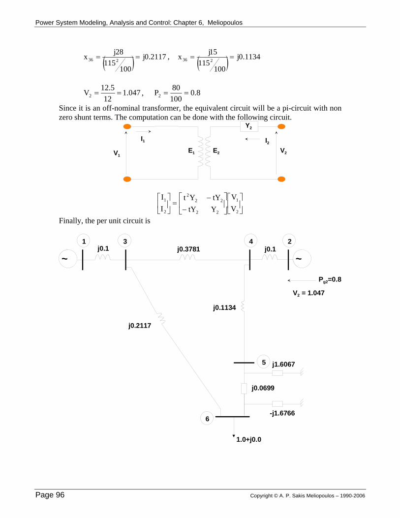
Power System Modeling, Analysis and Control: Chapter 6, Meliopoulos
( ) 2117.0j100
11528jx 236 == , ( ) 1134.0j
100115
15jx 236 ==
047.112
5.12V2 == , 8.010080P2 ==
Since it is an off-nominal transformer, the equivalent circuit will be a pi-circuit with non zero shunt terms. The computation can be done with the following circuit.
I1 I2
V1V2
Y2
E1 E2
⎥⎦
⎤⎢⎣
⎡⎥⎦
⎤⎢⎣
⎡
−−
=⎥⎦
⎤⎢⎣
⎡
2
1
22
222
2
1
VV
YtYtYYt
II
Finally, the per unit circuit is
~ ~
1 3 24
5
6
j0.0699
1.0+j0.0
Pg2=0.8
V2 = 1.047
j0.1j0.1 j0.3781
j0.2117
j0.1134
j1.6067
-j1.6766
Page 96 Copyright © A. P. Sakis Meliopoulos – 1990-2006

Power System Modeling, Analysis and Control: Chapter 6, Meliopoulos
c) the state variables of the system Assume bus 1 as a slack bus and bus 2 as a PV bus. Then, the system can be fully defined by the following state variables. [ ]654365432 VVVVx δδδδδ= d) power flow equation Real power flow equation: At bus 2: 2g244224
222P PVVgV)x(g −α−=
At bus 3: ( ) ( )3663443363431233P VVVgggV)x(g α+α−++=
At bus 4: ( ) ( )4554334224454342244P VVVVgggV)x(g α+α+α−++=
At bus 5: ( ) ( )56654455654255P VVVggV)x(g α+α−+=
At bus 6: ( ) ( ) 6d65563366563266P PVVVggV)x(g −α+α−+=
Reactive power flow equations: At bus 3: ( ) ( )3663443363431
233Q VVVbbbV)x(g β+β−++−=
At bus 4: ( ) ( )4554334224454342244Q VVVVbbbV)x(g β+β+β−++−=
At bus 5: ( ) ( )56654455654255Q VVVbbV)x(g β+β−+−=
At bus 6: ( ) ( )65563366563266Q VVVbbV)x(g β+β−+−=
Copyright © A. P. Sakis Meliopoulos – 1990-2006 Page 97

Power System Modeling, Analysis and Control: Chapter 6, Meliopoulos
Fall 2001, EE 4320
Solution for Homework Assignment #5 1. a)
8.0)sin(bVV)x(g 4224422P −δ−δ−= ( ))sin(bV)sin(bV)sin(bVV)x(g 13311633664334433P δ−δ+δ−δ+δ−δ−= ( ))sin(bV)sin(bV)sin(bVV)x(g 54455344332442244P δ−δ+δ−δ+δ−δ−= ( ))sin(bV)sin(bVV)x(g 655664554455P δ−δ+δ−δ−= ( ) 0.1)sin(bV)sin(bVV)x(g 566553663366P −δ−δ+δ−δ−= ( ) ( ))cos(bV)cos(bVVbbbV)x(g 63366433443363431
233Q δ−δ+δ−δ+++−=
( ) ( ))cos(bV)cos(bV)cos(bVVbbbV)x(g 5445534433244224454342244Q δ−δ+δ−δ+δ−δ+++−=
( ) ( ))cos(bV)cos(bVVbbbV)x(g 6556645544556s5654255Q δ−δ+δ−δ+++−=
( ) ( )cos(bV)cos(bVVbbV)x(g 566553663366563266Q δ−δ+δ−δ++−= )
where b13 = -10, b34 = -2.6448, b24 = -10, b36 = -4.7237, b45 = -8.8183, b56 = -14.3062, bs56 = -0.6224, bs65 = 0.5964. Based on the assumption of FDPF, the matrices B’ and B” are constant:
⎥⎥⎥⎥⎥⎥
⎦
⎤
⎢⎢⎢⎢⎢⎢
⎣
⎡
=
19.0299 14.3062- 0 4.7237- 0 14.3062- 23.1245 8.8183- 0 0
0 8.8183- 21.4631 2.6448- 10-4.7237- 0 2.6448- 17.3685 0
0 0 10- 0 10
B'
⎥⎥⎥⎥
⎦
⎤
⎢⎢⎢⎢
⎣
⎡
=
17.8371 14.3062- 0 4.7237-14.3062- 23.3693 8.8183- 0
0 8.8183- 21.4631 2.6448- 4.7237- 0 2.6448- 17.3685
B"
The iterative equations are as follows. ( ) [ ]V/)x(gB P
1'v1v −+ −δ=δ
( ) [ ]V/)x(gBVV Q1'v1v −+ −=
Page 98 Copyright © A. P. Sakis Meliopoulos – 1990-2006

Power System Modeling, Analysis and Control: Chapter 6, Meliopoulos
b) iteration #1 (Unit of angle is radian. Unit of voltage magnitude is pu)
,
⎥⎥⎥⎥⎥⎥⎥⎥⎥⎥⎥⎥
⎦
⎤
⎢⎢⎢⎢⎢⎢⎢⎢⎢⎢⎢⎢
⎣
⎡
−−
−
=
⎥⎥⎥⎥⎥⎥⎥⎥⎥⎥⎥⎥
⎦
⎤
⎢⎢⎢⎢⎢⎢⎢⎢⎢⎢⎢⎢
⎣
⎡
δδδδδ
0522.10171.10313.10189.10982.00529.0
0205.00236.0
0969.0
VVVV
6
5
4
3
6
5
4
3
2
iteration #2
,
⎥⎥⎥⎥⎥⎥⎥⎥⎥⎥⎥⎥
⎦
⎤
⎢⎢⎢⎢⎢⎢⎢⎢⎢⎢⎢⎢
⎣
⎡
−−
−
=
⎥⎥⎥⎥⎥⎥⎥⎥⎥⎥⎥⎥
⎦
⎤
⎢⎢⎢⎢⎢⎢⎢⎢⎢⎢⎢⎢
⎣
⎡
δδδδδ
0311.19978.00196.10103.10861.00428.0
0291.00198.0
1032.0
VVVV
6
5
4
3
6
5
4
3
2
iteration #3
⎥⎥⎥⎥⎥⎥⎥⎥⎥⎥⎥⎥
⎦
⎤
⎢⎢⎢⎢⎢⎢⎢⎢⎢⎢⎢⎢
⎣
⎡
−−
−
=
⎥⎥⎥⎥⎥⎥⎥⎥⎥⎥⎥⎥
⎦
⎤
⎢⎢⎢⎢⎢⎢⎢⎢⎢⎢⎢⎢
⎣
⎡
δδδδδ
0357.10018.10216.10121.10883.00433.0
0306.00198.0
1057.0
VVVV
6
5
4
3
6
5
4
3
2
Copyright © A. P. Sakis Meliopoulos – 1990-2006 Page 99

Power System Modeling, Analysis and Control: Chapter 6, Meliopoulos
Solution: a) Assume that bus 1 is a slack bus.
State variables: V2 and δ2So, minimum equations are
10.8V2sinδ2 + 1.0 = 0 10V2
2 –10.8V2cosδ2 + 0.6 = 0 b) 8.10B' =
2.98.0*28.10B" =−=
[ ] ⎥⎦
⎤⎢⎣
⎡∆−δ=δ
−ν+ν
2
1'2
12 V
PB
[ ] ⎥⎦
⎤⎢⎣
⎡∆−=
−ν+ν
2
1"2
12 V
PBVV
c) Initial condition: V2 = 1.0 and δ2 = 0.0 1st iteration: δ2 = -0.0926 V2 = 1.0217 2nd iteration: δ2 = -0.0908 V2 = 1.0162
Page 100 Copyright © A. P. Sakis Meliopoulos – 1990-2006