Embed Size (px)
Citation preview
AN INCREMENTAL TOTAL LAGRANGIAN FORMULATION FOR
GENERAL ANISOTROPIC SHELL-TYPE STRUCTURES
by
Chung-Li Liao
Dissertation submitted to the Faculty of the
Virginia Polytechnic Institute and State University
in partial fulfillment of the requirements for the degree of
DOCTOR OF PHILOSOPHY
in
Engineering Mechanics
APPROVED:
Dr. J. N. Reddx;:gtamnan
Dr. M. S. Cramer Dr:'R: T. Haftka
1-·<W" -" '''<
Dr. R. A. Heller / Dr. L. Meirovitch
June, 1987
Blacksburg, Virginia
AN INCREMENTAL TOTAL LAGRANGIAN FORMULATION FOR
GENERAL ANISOTROPIC SHELL-TYPE STRUCTURES
by
Chung-Li Liao
ABSTRACT
Based on the principle of virtual displacements, the incremental equations of motion
of a continuous medium are formulated by using the total Lagrangian description. After
linearization of the incremental equations of motion, the displacement finite element
model is obtained, which is solved iteratively. From this displacement finite element
model, four different elements, i.e. degenerated shell element, degenerated curved beam
element, 3-D continuum element and solid-shell transition element, are developed for the
geometric nonlinear analysis of general shell-type structures, anisotropic as well as
isotropic. Compatibility and completeness requirements are stressed in modelling the
general shell-type structures in order to assure the convergence of the finite-element
analysis. For the transient analysis Newmark scheme is adopted for time discretization.
An iterative solution procedure, either Newton-Raphson method or modified
Riks/Wempner method, is employed to trace the nonlinear equilibrium path. The latter
is also used to perform post-buckling analysis. A variety of numerical examples are pre-
sented to demonstrate the validity and efficiency of various elements separately and in
combination. The effects of boundary conditions, lamination scheme, transverse shear
deformations and geometric nonlinearity on static and transient responses are also in-
vestigated. Many of the numerical results of general shell-type structures presented here
could serve as references for future investigations.
ACKNOWLEDGEMENTS
The author would like first to express sincere appreciation to his major advisor,
Professor J. N. Reddy, for the constant guidance and support. Professor Reddy's wide
and solid professional knowledge has truly made the author's learning rewarding. The
author is also obliged to Dr. M. S. Cramer, Dr. R. T. Haftka, Dr. R. A. Heller and Dr.
L. Meirovitch for serving as members of the committee and reviewing this dissertation.
Special thanks are due to Professor J. H. Sword for his help in providing computer funds
during the author's study at Virginia Tech.
I want to give my deep gratitude to my beloved family for their love, encouragement
and sacrifice during the past years. My teachers are also acknowledged for their in-
struction and inspiration.
Finally, I am pleased to thank the friendship of my fellow students here and my best
friend Mr. Y. K. Yang.
11
Table of Contents
Page
ABSTRACT
ACKNOWLEDGEMENTS . . . . . . . . . . . . . . . . . . . . . . . . . . . . . . . . . . . . . . . . . . . . . . . 11
1. INTRODUCTION .................................................. .
1.1 Motivation . . . . . . . . . . . . . . . . . . . . . . . . . . . . . . . . . . . . . . . . . . . . . . . . . .... .
1.2 Review of the Literature . . . . . . . . . . . . . . . . . . . . . . . . . . . . . . . . . . . . . . . . . . . . . 2
1.3 Present Study . . . . . . . . . . . . . . . . . . . . . . . . . . . . . . . . . . . . . . . . . . . . . . . . . . . . 7
2. FORMULATION OF THE INCREMENTAL EQUATIONS OF MOTION
BY THE TOTAL LAGRANGIAN DESCRIPTION . . . . . . . . . . . . . . . . . . . . . . . . . . 9
2.1 Introduction . . . . . . . . . . . . . . . . . . . . . . . . . . . . . . . . . . . . . . . . . . . . . . . . . . . . . 9
2.2 Principle of Virtual Displacements . . . . . . . . . . . . . . . . . . . . . . . . . . . . . . . . . . . . . 10
2.3 Total Lagrangian Formulation . . . . . . . . . . . . . . . . . . . . . . . . . . . . . . . . . . . . . . . . 13
2.4 Linearization of Incremental Equations of Motion . . . . . . . . . . . . . . . . . . . . . . . . . . 16
3. DISPLACEMENT FINITE ELEMENT MODEL . . . . . . . . . . . . . . . . . . . . . . . . . . . . 18
3.1 Introduction . . . . . . . . . . . . . . . . . . . . . . . . . . . . . . . . . . . . . . . . . . . . . . . . . . . . . 18
3.2 Finite-Element Discretization . . . . . . . . . . . . . . . . . . . . . . . . . . . . . . . . . . . . . . . . . 18
3.3 Finite-Element Model . . . . . . . . . . . . . . . . . . . . . . . . . . . . . . . . . . . . . . . . . . . . . . 19
3.4 Newmark Scheme for Time Discretization . . . . . . . . . . . . . . . . . . . . . . . . . . . . . . . . 20
4. SOLUTION PROCEDURES . . . . . . . . . . . . . . . . . . . . . . . . . . . . . . . . . . . . . . . . . . . 22
4.1 Introduction . . . . . . . . . . . . . . . . . . . . . . . . . . . . . . . . . . . . . . . . . . . . . . . . . . . . . 22
4.2 Newton-Raphson Method ........................................... 22
4.3 Modified Rilcs-Wempner Method . . . . . . . . . . . . . . . . . . . . . . . . . . . . . . . . . . . . . . 25
4.4 Convergence Criteria . . . . . . . . . . . . . . . . . . . . . . . . . . . . . . . . . . . . . . . . . . . . . . . 33
5. ELEMENT DEVELOPMENT . . . . . . . . . . . . . . . . . . . . . . . . . . . . . . . . . . . . . . . . . . 35
5.1 Introduction . . . . . . . . . . . . . . . . . . . . . . . . . . . . . . . . . . . . . . . . . . . . . . . . . . . . . 35
5.2 Degenerated 3-D Shell Element . . . . . . . . . . . . . . . . . . . . . . . . . . . . . . . . . . . . . . . 35
ill
5.3 Degenerated Curved Beam Element .................................... 47
5.4 Three-Dimensional Continuum Element . . . . . . . . . . . . . . . . . . . . . . . . . . . . . . . . . 56
5.5 Solid-to-Shell Transition Element . . . . . . . . . . . . . . . . . . . . . . . . . . . . . . . . . . . . . . 62
6. SAMPLE ANALYSIS . . . . . . . . . . . . . . . . . . . . . . . . . . . . . . . . . . . . . . . . . . . . . . . . . 70
6.1 Introduction . . . . . . . . . . . . . . . . . . . . . . . . . . . . . . . . . . . . . . . . . . . . . . . . . . . . . 70
6.2 Static Analysis . . . . . . . . . . . . . . . . . . . . . . . . . . . . . . . . . . . . . . . . . . . . . . . . . . . . 70
6.2.1 Plate and Shell Structures . . . . . . . . . . . . . . . . . . . . . . . . . . . . . . . . . . . . . . . . 70
6.2.2 Beam Structures . . . . . . . . . . . . . . . . . . . . . . . . . . . . . . . . . . . . . . . . . . . . . . 80
6.2.3 Stiffened Plates and Shells . . . . . . . . . . . . . . . . . . . . . . . . . . . . . . . . . . . . . . . 94
6.2.4 Applications of Solid-Shell Transition Element . . . . . . . . . . . . . . . . . . . . . . . 112
6.2.5 General Shell-Type Structures . . . . . . . . . . . . . . . . . . . . . . . . . . . . . . . . . . . 119
6.3 Transient Analysis . . . . . . . . . . . . . . . . . . . . . . . . . . . . . . . . . . . . . . . . . . . . . . . . 140
6.3.1 Plate and Shell Structures . . . . . . . . . . . . . . . . . . . . . . . . . . . . . . . . . . . . . . . 142
6.3.2 Beam Structures . . . . . . . . . . . . . . . . . . . . . . . . . . . . . . . . . . . . . . . . . . . . . 145
6.3.3 Stiffened Plates and Shells . . . . . . . . . . . . . . . . . . . . . . . . . . . . . . . . . . . . . . 149
6.3.4 Applications of Solid-Shell Transition Element . . . . . . . . . . . . . . . . . . . . . . . 155
6.3.5 General Shell-Type Structures . . . . . . . . . . . . . . . . . . . . . . . . . . . . . . . . . . . 155
7. CONCLUSIONS AND RECOMMENDATIONS ........................... 163
7 .1 Summary and Conclusions . . . . . . . . . . . . . . . . . . . . . . . . . . . . . . . . . . . . . . . . . . 163
7.2 Recommendations . . . . . . . . . . . . . . . . . . . . . . . . . . . . . . . . . . . . . . . . . . . . . . . . 164
REFERENCES . . . . . . . . . . . . . . . . . . . . . . . . . . . . . . . . . . . . . . . . . . . . . . . . . . . . . . . 165
APPENDIX . . . . . . . . . . . . . . . . . . . . . . . . . . . . . . . . . . . . . . . . . . . . . . . . . . . . . . . . . . 171
VITA . . . . . . . . . . . . . . . . . . . . . . . . . . . . . . . . . . . . . . . . . . . . . . . . . . . . . . . . . . . . . . . 175
iv
CHAPTER 1
INTRODUCTION
1.1 Motivation
In the practical analysis of shell-type structures, such as stiffened plates and shells,
folded plates, arch dams and foundations, turbine blades mounted on a shaft etc., by fi-
nite element method we need to employ shell elements in conjunction with three-
dimensional beam elements and/or 3-D continuum elements to model the structures
effectively and accurately. Also transition elements are preferred to model shell inter-
sections and solid-to-shell transition regions without invoking the constraint equations.
These elements must satisfy compatibility and completeness requirements in order to
assure the convergence of the finite-element analysis.
Traditionally the formulations of shell and beam elements have been based on various
shell and beam theories. The detailed governing equations may vary considerably de-
pending upon the approximation used. This accounts for the existence of several differ-
ent beam and shell finite elements with varying degree of accuracy and applicability.
These elements are not useful for nonlinear, large displacement, analysis of structures
since the elements become distorted and the changes in the structural geometries cannot
be accounted for accurately. Remedial formulations of shell and beam elements [ 11, 16]
have been proposed in which no specific shell and beam theories are employed; instead,
the geometry and the displacement fields of the structure are directly discretized and in-
terpolated as in the analysis of continuum problems. These general shell elements and
three-dimensional beam elements are degenerated from a three-dimensional
isoparametric element by imposing some geometric and static contraints to satisfy the
assumptions of a shell or beam theory. Since the same interpolation functions are em-
ployed for the beam element as in the formulation of the shell element, the beam and
shell elements are compatible and can be used together effectively to model stiffened
plates and shells. Both shell and beam elements can have a variable number of nodes,
and the shell element can be modified as transition elements to model shell intersections
or solid-to-shell transition regions. Such formulations would appear to be especially
applicable to material and geometrical nonlinear analysis of shell-type structures in
which large displacements and rotations are experienced.
A brief review of the literature is presented below to indicate the directions of recent
research efforts in the analysis of general shell-type structures. The review is intended
to provide a background for the present study. Due to the increasing applications of
layered composite shell-type structures in engineering the present study will be oriented
particularly toward the analysis of the laminated composite structures.
1.2 Review of the Literature
A large number of different finite elements have been formulated for the static and
dynamic analyses of plate and shell problems, anisotropic as well as isotropic. In these
developments, basically three approaches have been followed. In the first approach a
plate or shell theory is used as the starting point of the finite element formulation. This
plate or shell theory is derived from the three-dimensional continuum mechanics
equations by various static and kinematic assumptions. Using variational formulations
based on these theories various finite element models have been developed; namely, dis-
placement, hybrid and mixed models [1-5]. In the second approach 3-D elements based
on three dimensional elasticity are used [6-10]. In the third approach, isoparametric ele-
ments with independent rotational and translational displacements degrees of freedom
2
are employed and the geometry and displacement fields are directly discretized and in-
terpolated as in the analysis of continuum problems without applying any specific shell
or plate theory. The third approach was originally introduced by Ahmad et al. [11] for
the linear analysis of moderately thick and thin shells and has been applied to the non-
linear analysis of plates and shells by Ramm [ 12], Krakeland [ 13 ], Chang [ 14], Bathe [ 15],
Bolourchi [16], Chao and Reddy [17], among others. The advantage of elements based
on the third approach is their inherent generality compared to 2-D shell or plate ele-
ments in the first approach and simplicity compared to fully 3-D elements. They can
account for full geometric non-linearities in contrast to 2-D elements based on shell or
plate theory in the first approach, while possessing computational simplicity over a fully
3-D element, where the use of several nodes across the shell thickness ignores the well-
known fact that even for thick shells the 'normals' to the middle surface remain almost
straight after deformation.
Curved beams are used extensively nowadays as stand alone or as reinforcing mem-
bers of thin shells. When solving the problems of shells with stiffeners by the finite ele--- - --- --- ·--- - ----- ·-·>--·- _. .. - - - . '
ment method, a beam element whose displacement pattern is compatible with that of the ·----- -- . --·- ... --- ' - -
shell is required. )n analyzing eccentrically stiffened cylindrical shell, Kohnke et al. [ 18]
proposed a 16 d.o.f. isotropic beam finite element which has displacements compatible
with the cylindrical shell element from which the beam element is reduced. Rao and
Venkatesh have presented a laminated anisotropic curved stiffener element with 16 d.o.f.
[19] which is degenerated from a laminated anisotropic rectangular shallow thin shell
element with 48 d.o.f. [20] in order to achieve compatibility all along the shell-stiffener
junction line. This compatible curved stiffener element [ 19] and the. rectangular shell el-
ement [20] have been used in Ref.[21) to solve problems of laminated anisotropic shells
stiffened by laminated anisotropic stiffeners. Rao and Venkatesh [22] later presented the
3
analysis of laminated anisotropic shells of revolution reinforced by laminated anisotropic
stiffener using 48 d.o.f. doubly curved quadrilateral shell of revolution element [23),
where the stiffener elements again are degenerated from the shell element in [23). The
element matrices of the beam element and the element matrices of the shell are super-
posed after both have been suitably transformed. Thus no any additional degrees of
freedom are introduced when compared with non-stiffened shell structures.
One alternative method of taking into account the presence of stiffening beams and
ribs attached to shell structures is to approximate these members by the same element
types as used for the shell [24-25]. This procedure has the disadvantage of introducing
a substantial number of additional nodes and nodal displacement unknowns.
A variable thickness curved beam and shell stiffening element with transverse shear
deformation was developed by Ferguson and Clark [26). In this work, a family of 2-D
and 3-D beam elements are presented which are double degeneration of a fullly 3-D
isoparametric continuum element. They exhibit such characteristics as displacement
compatibility with Ahmad thick shell elements [11), transverse shear and variable thick-
ness properties. Also, with the introduction of offsets in the basic element formulation,
2-D and 3-D stiffeners and curved beams of general cross-section can be modelled.
In References [ 18), [21] and [22) for the analysis of stiffened shell structures, the shell
and beam elements are all based on the classical thin shell and beam theories. Therefore,
the transverse shear deformation is neglected. Bathe and Bolourchi [16) employed
Ahmad thick shell elements in conjunction with degenerated 3-D beam elements to
model an isotropic stiffened plate in which the transverse shear deformations are in-
cluded. But in all of these works only linear static analysis is considered.
4
The development of the governing finite element equations for the nonlinear response
of a solid body under external loads has been given by numerous investigators
[14-17,27-33]. Finite elememt analyses of the large displacement theories are based on
the principle of virtual work or the associated principle of stationary potential energy.
Horrigmoe and Bergan [27] presented classical variational principles for non-linear
problems by considering incremental deformations of a continuum. A survey of various
principles in incremental form in different reference configurations, such as the total
Lagrangian and the updated Lagrangian formulations, is presented by Wunderlich [28].
In the total Lagrangian description, all static and kinematic variables are referred to the
initial configuration. In the updated Lagrangian description all variables are referred to
the current ~onfiguration.
By using a geometrically nonlinear formulation, the finite element method has been
used in analyzing arch and shell instability problems [34-37]. A special numerical tech-
nique must be adopted to trace the path of the load-deflection curve near the limit point
(critical buckling load) and in the post-buckling region because the stiffness matrix at the
vicinity of the limit point is nearly singular and the descending branch of the load-
deflection curve in the post-buckling region is characterized by a negative-definite
stiffness matrix. This means that the structure can withstand only a decreasing load after
buckling. Many methods have been proposed to overcome this problem. Among these
are the simple method of suppressing equilibrium iterations [39,40], the introduction of
artificial spring [34), the displacement control method [41,42), and the "constant-arc-
length method" of Riks [43] and Wempner [46). Reviews of these most commonly used
techniques are contained in References [44,45]. Among these methods the modified
Riks-Wempner method appears to be the most effective in conjunction with the finite
element method. Many investigators [43-48] have already used this method in its original
5
or modified versions to determine the pre- and post-buckling behaviors of various types
of structures, such as arch, shell and dome. In most of these works only isotropic mate-
rial is considered. Very few works of nonlinear buckling analysis for laminated composite
structures [65] are reported in the literature.
In many industrial aplications the structures are composed of three-dimensional solid
continuum with the thin shell-like portions connected to them. In modelling such struc-
tures 3-D solid elements and shell elements are employed, for three-dimensional solid
and shell-like portions. Since the nodal degrees-of-freedom for these two types of ele-
ments are incompatible with each other, the connections of shell elements to the solid
elements present considerable difficulty. Three possible approaches to model these
practical structures exist: ( 1) Discretize shell-like portions of the structure with solid el-
ements also. This approach may be computationally expensive and impractical. Also it
may lead to erroneous results for thin sheet metal structures due to shear locking phe- .
nomenon or the stiffness matrix becoming ill-conditioned. (2) Use multipoint constraint
equations for connecting three-dimensional solid elements and shell elements. (3) De-
velop transition elements which can provide proper connections between the two
portions of the structure modelled with three-dimensional solids and the curved shell el-
ements. The transition elements for three-dimensional stress analysis can be found in
the works by Bathe and his colleagues [15,16,49) and Surana [50,51]. The transition ele-
ment possesses the properties of both three-dimensional solid element and degenerated
3-D shell element which are all derived using three-dimensional elasticity equations.
Hence the compatibility between transition element and solid element (or shell element)
is preserved. These transition elements can be employed to model: (1) solid-to-shell
transition regions, in which the transition element provides connections between the two
portions of the structure being modelled, namely, the 3-D solid elements and shell ele-
6
ments, (2) the intersections of different shell surfaces. The major advantage of employing
transition element is to eliminate the constraint equations which otherwise need be in-
cluded at these transition regions. Although the transition element has been used for
linear and geometrically nonlinear static analysis of isotropic material, the application
for linear and nonlinear static and transient analyses of laminated anisotropic shell-type
structures has not yet been reported.
The degenerated 3-D shell element has been investigated for geometrically nonlinear
analysis of isotropic and laminated anisotropic shells [14,16,17,33]. From the review of
the literature it appears that the geometrically nonlinear analyses of isotropic and lami-
nated anisotropic stiffened shells and shell-type structures with discontinuous geometries
have not received the attention they deserve. Most practical structures involve stiffened
panels and pressure vessels with geometric discontinuities (e.g., windows, doors, holes,
etc.), and experience geometric nonlinearities. The problem of calculating stresses, fre-
quencies and buckling loads in composite structures are magnified by the anisotropy and
bending-stretching coupling. Motivated by these observations the following program
of research was undertaken.
1.3 Present Study
The present study is directed to deal with the following topics:
• Development of incremental total Lagrangian formulations for shell, beam and
three-dimensional solid elements. Also, the development of the transition elements
used to model solid-to-shell transition regions and shell intersections.
• Development of a numerical algorithm based on the incremental total Lagrangian
formulation and the Newton-Raphson method for geometrically nonlinear static and
7
transient analyses of isotropic and layered anisotropic curved beams, arches, shells,
stiffened shells and the other practical shell-type structures.
• Buckling and post-buckling analysis of isotropic and layered anisotropic arches,
shells and stiffened shells by using the modified Riks-Wempner method.
The incremental formulation for nonlinear analysis by using total Lagrangian de-
scription is presented in Chapter 2 and the associated finite element model is described
in Chapter 3. Chapter 4 contains the iterative solution procedures, Newton-Raphson
method and modified Riks-Wempner method, which are used to solve the nonlinear fi-
nite element equations. The developments of degenerated 3-D shell element, degener-
ated curved beam element, 3-D solid element and solid-shell transition element
incorporated with the incremental formulation are presented in Chapter 5. Chapter 6
contains the discussions of numerical results of linear and geometrically nonlinear static
and transient analyses of isotropic and laminated composite beams, shells, stiffened
shells and some general shell-type structures. Comparisons of the present results with the
results available in the literature show very good agreements. Many numerical results
of stiffened shells and some general shell-type structures could serve as references for
future investigations. In Chapter 7 a summary, conclusions and recommendations of the
present study are included.
8
CHAPTER 2
FORMULATION OF THE INCREMENTAL EQUATIONS OF MOTION BY
THE TOTAL LAGRANGIAN DESCRIPTION
2. 1 Introduction
In the linear description of the motion of solid bodies it is assumed that the dis-
placements are infinitely small and that the material is linearly elastic. In addition we
assume the configuration and the nature of the boundary conditions remain unchanged
during the entire deformation process. These assumptions imply that the displacement
vector { U} is a linear function of the applied load vector {R}. The evaluation of element
matrices and load vectors are performed over the original volume of the finite elements
and are assumed to be constant and independent of the element displacements.
The nonlinearity in solid mechanics arises from two distinct sources. One is due to
the kinematics of deformation of the body and the other from the constitutive behavior
(i.e., stress-strain relations). The analyses in which the first type of nonlinearity is con-
sidered are called geometrically nonlinear analyses, and those in which the second type
is considered are called materially nonlinear analyses. The geometrically nonlinear
analysis can be subclassified into two cases : (i) large displacements, large rotations and
small strains (ii) large displacements, large rotations and large strains. In the first case
it is assumed that the rotations of line elements are large, but their extensions and
changes of angles between two line elements are small. In the second case the extension
of a line element and angle changes between two line elements are large, and rotations
of a line element are also large.
9
In the present study the first type of geometrical nonlinearity is considered, and it is
assumed that the material is linear elastic.
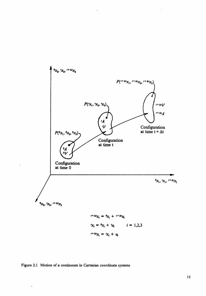
Consider the motion of a body in a fixed Cartesian coordinate system as shown in
Fig. 2.1 and assume that the body can experience large displacements and rotations.
We wish to determine the configuration of the body for different times and loads. The
formulation to be described assumes that the solutions for the kinematic and static var-
iables for all time steps from time 0 to time t, inclusive, have been obtained, and that the
solution for time t + ll.t is pursued next. Hence in the present formulation we follow all
particles of the body as it deforms from the initial configuration to the final configura-
tion. This type of description is called the Lagrangian description, which differs from the
Eulerian description usually used in the analysis of fluid mechanics problems. There are
various methods used to describe motion of a continuum in Newtonian mechanics as
described in References [38,52).
In the Lagrangian description of motion all variables are referred to a reference
configuration, which can be the initial configuration or any other convenient configura-
tion. The description in which all variables are referred to the current configuration is
called the updated Lagrangian description [31,3 2) and the one in which all variables are
refered to the initial configuration is called the total Lagrangian description [ 17 ,33).
2.2 Principle of Virtual Displacements
Since the displacement based finite element procedure will be employed for numerical
solution, the principle of virtual displacements is used to express the equilibrium of the
body in the configuration at time t + /l.t. The principle of virtual displacements requires
that
10
Configuration at time 0
P(t+4tx r+4rx r+4rx) I• l• 3
Configuration at time t
t+"'x, = •x, + r+4tu,
'x, = 0x, + 'u,
t+4tx1 = 'x, + u,
Configuration at time t + .6.t
; = 1,2,3
Figure 2.1 Motion of a continuum in Cartesian coordinate systems
II
(2.1)
where i+t.t't,1 = the Cartesian components of the Cauchy stress tensor at time t + l::..t.
(The Cauchy stresses are always referred to the configuration in which
i+oAJ = the Cartesian components of the infinitesimal strain tensor associated
with the displacements u, in going from the configuration at time t to the
nfi . . . 1 ( ou1 ou1 ) which co igurat1on at trme t + l::..t , i.e. ,+o,e;1 = -2 .::i + Ut+dtX} ot+6tX;
are also referred to this unknown configuration at time t + i::..t,
1+o1x1 = Cartesian components of a point in configuration at time t + l::..t , the left
superscript refers to the configuration of the body,
and
(2.2)
:a:rk and :t~~ are the components of the externally applied surface and body .force vec-
tors respectively, ouk is a virtual variation in the current displacement components
i+t.tuk, and o,+o1e11 are the virtual variations in strains.
Equation (2.1) cannot be solved directly since the co!lfiguration at time t + l::..t is
unknown. This is an important difference compared with the linear analysis in which
we assume that the displacements are infinitesimally small so that the configuration of
the body does not change. In a large deformation analysis special attention must be
given to the fact that the configuration of the body is changing continuously. This
change in configuration can be dealt with by defining auxiliary stress and strain meas-
12
ures. The objective in their definition is to express the internal work in eqn. (2.1) in terms
of an integral over a volume that is known. The stress and strain measures that we shall
use are the 2nd Piela-Kirchhoff stress tensor and the Green-Lagrange strain tensor.
An approximate solution of eqn. (2.1) can be obtained by referring all variables to
a previously calculated known equilibrium configuration and linearizing the resulting
equation. This solution is then improved by iteration. In principle, any one of the al-
ready calculated equlibrium configurations could be used. In practice total Lagrangian
{T. L.) and updated Lagrangian (U. L.) formulations are choosed. In the T. L. formu-
lation all static and kinematic variables are referred to the initial configuration at time
0. The U. L. formulation is based on the same procedures that are used in the T. L.
formulation, but all static and kinematic variables are referred to the configuration at
time t. Both the T. L. and U. L. formulations include all kinematic nonlinear effects due
to large displacments, large rotations and large strains. In the present study the total
Lagrangian formulation is adopted.
2.3 Total Lagrangian Formulation
In the formulation all variables in eqns. (2.1) and (2.2) are referred to the initial
configuration at time 0 of the body. The applied forces in eqn. (2.2) are evaluated using
t+t:..tp t+t:..tr t+t:..tdV _op t+t:..tr odV t+t:..tlk - Olk (2.3)
when the loading is deformation-independent and can be specified prior to the incre-
mental analysis.
13
The volume integral of Cauchy stresses times variations in infinitesimal strains in eqn.
(2.1) can be transformed to give [38]
(2.4)
where t+~SIJ = Cartesian components of the 2nd Piela-Kirchhoff stress tensor
as
corresponding to configuration at time t + tit but measured in the con-
figuration at time 0.
t+&Je,1 = Cartesian components of the Green-Lagrange strain tensor in the
configuration at time t + tit , referred to the configuration at time 0, and
t+Me are defined as t+Me = ~t+Mu + t+Mu + t+Mu t+Mu ) 0 lj 0 lj 2' 0 IJ 0 j,I 0 k,I 0 kJ t
i)t+Mu1
fflx j 1+61u1 = components of displacement vector from initial position at time 0 to
configuration at time t + tit, 1H 1u, = 1+Mx, - 0x,
The 2nd Piela-Kirchhoff stress tensor referred to the configuration at time 0 is defined
Op t+&tS _ __ Or t+Mt,, t+•o;x1,
0 lj - t+Mp t+&rl,s u •
and is energetically conjugate to the Green-Lagrange strain tensor. Also the Cauchy
stress tensor is energetically conjugate to the infinitesimal strain tensor. Hence, the total
internal virtual work can be calculated using as stress measures either the Cauchy or the
2nd Piela-Kirchhoff stress tensors provided the conjugate strain tensors are employed
and the integrations are performed over the current and original volumes, respectively.
The relation of eqn. (2.4) explains that the 2nd Piela-Kirchhoff stress and Green-
Lagrange strain tensors are energetically conjugate.
14
Substituting the relations in eqn. (2.3) and (2.4) into eqns. (2.1) and (2.2), the fol-
lowing equilibrium equation for the body in the configuration at time t + tit but referred
to the configuration at time 0 is obtained
r 1+ Ms ~1+ M odV _ 1+ MR Jov o IJ o 0elJ - (2.5)
where t+t.tR is calculated using
(2.6)
Since the stresses '+AJS,1 and strains '+AJe,1 are unknown, the following incremental
decompositions are used
(2.7)
(2.8)
where JSIJ and Je,1 are the known 2nd Piela-Kirchhoff stresses and Green-Lagrange strains
in the configuration at time t. Using the definition of the Green-Lagrange strain tensor
and 'H'u, = •u, + u, ,where u, = the increment in displacement components, it follows
that
(2.9)
where
(2.10)
= linear part of strain increment 0e11
15
(2.11)
= nonlinear part of strain increment 0e,1
The incremental 2nd Piela-Kirchhoff stress components 0SIJ are related to the incre-
mental Green-Lagrange strain components 0e1J using the constitutive tensor 0C11,. , i.e.
(2.12)
Using eqns. (2.7) - (2.12), eqn. (2.5) can be written as
(2.13)
which respresents a nonlinear equilibrium equation for the incremental displacements
2.4 Linearization of Incremental Equations of Motion
The solution of eqn. (2.13) cannot be calculated directly, since they are nonlinear in
the displacement increments. Approximate solution can be obtained by assuming that
0e1J = 0elJ in eqn. (2.13). This means that, in addition to using 00e11 = o0eu , the incremental
constitutive relation employed is
Hence, in the T. L. formulation the approximate equation to be solved is
(2.14)
16
In dynamic analysis, the applied body forces include inertial forces. In this case we
have
S t+M t+llf.. ~t+M t+MdV _ f 0 t+Mu··1 ~t+Mu1 OdV r+Mv p u1 u u1 - Jov p o (2.15)
and hence the mass matrix can be evaluated using the initial configuration of the body.
Using Hamilton's principle we obtain the equations of motion of the moving body at
time t + tl.t in the variational form as
fol' Op t+dtu··, ~t+Mu, OdV + fol' 0C1,1n oen ~ e OdV + r 'S ~ TI OdV -JI 0 JI , Oo lj JOv 0 lj Oo•!ij -
(2.16)
17
CHAPTER 3
DISPLACEMENT FINITE ELEMENT MODEL
3. 1 Introduction
Based on the principle of virtual displacements the incremental equations of motion,
eqn. (2.16) presented in Chapter 2, can be used to develop general nonlinear displace-
ment finite element model. The generalized displacements are the primary variables in
the governing finite element equations.
The basic steps in deriving the governing finite element equations include: ( 1) The
selection of proper interpolation functions. (2) The interpolating of the element dis-
placements and coordinates with these functions. (3) Substituting the displacement and
geometry fields into the governing equations of motion. Then invoking the principle of
virtual displacements for each of the nodal point displacements in tum and the govern-
ing finite element equation are obtained. Only a single element of a specific type is con-
sidered in the above derivation. The final algebraic equations of motion for an
assemblage of elements are obtained by assembling the governing equations of motion
of each element.
3.2 Finite-Element Discretization
It is important that the coordinates and displacements are interpolated using the
same interpolation functions so that the displacement compatibility across element
boundaries can be preserved in all configurations. Hence II
'x = L in '.rl I k-l 'f'k I
t+M 11 t+M k Xt = L <f>k X;
k=l i = 1, 2, 3 (3. 1)
18
t n t k u1 = L <l>k u1 ,
k=l i = 1, 2, 3 (3.2)
where the right superscript k indicates the quantity at nodal point k, <p* is the interpo-
lation function corresponding to nodal point k, and n is the number of element nodal
points.
3.3 Finite-Element Model
Using eqns. (3.1) and (3.2) to evaluate the displacement derivatives required in the
integrals, eqn. (2.16) becomes,
(3.3)
where {6•} is the vector of nodal incremental displacements from time t to time t + 6t
in one element, and 01M]t+111{Li•}, 01Kd{6•}, &[KNL]{6•}, and J{F} are obtained by evaluat-
ing the integrals
rOv Op t+Mu··, S::t+Mu, OdV r c e I:: e OdV r 'S I:: n OdV JI o , JOv o ijn o ,. oo ti , JOv o ii Oo·11j
and Jov JSIJ 00e1J 0dV respectively, i.e.
(3.4)
(3.5)
(3.6)
" ci{F} = Jov ci[BJT ci{S} 0dV (3.7)
19
In the above equations, J[BL] and J[BNL] are linear and nonlinear strain-displacement
transformation matrices, 0[ q is the incremental stress-strain material property matrix, . J[S] is a matrix of 2nd Piela-Kirchhoff stress components, J{S} is a vector of these
stresses, and '[H] is the incremental displacement interpolation matrix. All matrix ele-
ments correspond to the configuration at time t and are defined with respect to the
configuration at time 0.
It is important to note that eqn. (3.3) is only approximation to the actual solution
to be solved in each time step, i.e. eqn. (2.13). Therefore it may be necessary to iterate
in each time step until eqn. (2.13) is satisfied to a required tolerance.
Note that the finite element equations (3.3) are 2nd order differential equations in
time. In order to obtain numerical solutions at each time step, eqn. (3.3) needs to be
converted to algebraic equations.
3.4 Newmark Scheme for Time Discretization
In this study the Newmark integration scheme is used to convert the ordinary dif-
ferential equations in time to algebraic equations. In the Newmark scheme, displace-
ments and velocities are approximated by
1+M{~} = '{~} + '{A} ~t + [(+ -p) '{Li} + p 1+M{,!i}) (~1)2
(3.8)
where a = f, p = ! for the constant average acceleration method and ~t is the time
. step. Rearranging eqns. (3.3) and (3.8), we obtain
A A
ci[KJ {~} = t+M{R} (3.9)
20
where {d} = vector of nodal incremental displacements at time t = t+d'{d} - '{d}, and .
J[K] = Clo J[M] + J[KL) + J[KNL] . t+dt{R} = t+M{R} - J{F} + J[M] (a, '{~} + ~ 1{Li})
1 1 Clo = ~(dt)2 , a, = Clo dt , ~ = 2p - 1
Once eqn. (3.9) is solved for {d} at time t + dt, the acceleration and velocity vectors
are obtained by
(3.10)
where a3 = (I - a) dt , a.a = a dt
21
CHAPTER4
SOLUTION PROCEDURES
4.1 Introduction
In Chapter 3 we obtained the final governing finite element equations to be solved
at each time step t, i.e. eqn. (3.9), for each element. For an assemblage of elements the
governing equations are constructed by assembling eqn. (3.9) of each element together.
We noted in Chapter 3 that eqn. (3.3) is only linearized approximation to the actual
governing equation of motion, eqn. (2.13), and so is eqn. (3.9). Therefore it is necessary
to solve eqn. (3.9) iteratively at each time step until eqn. (2.13) is satisfied to a required
tolerance. Two iterative procedures are often used in the finite element analysis of non-
linear problems. One is the direct iteration, also known as the Picard method. The other
is the Newton-Raphson method. Here the Newton-Raphson method is adopted.
4.2 Newton-Raphson Method
The right-hand side of eqn. (3.9) corresponds to the out-of-balance load vector which
is not yet balanced by element stresses at time t when the continuum moves from con-
figuration at time t to one at time t + .1t. Hence an increment in the nodal point dis-
placements is required. This updating of the nodal displacements in the iteration is
continued until the out-of-balance loads are small.
Assume that in the iterative solution we have evaluated i+M{~}<H> . Then by the
Taylor series expansion and neglecting the 2nd and higher-order terms we obtain the
equation to be solved at the i-th iteration as
22
\.-I , 1..( 1'·
. . = _ J[K] {A}(l-1> + 1+M{R}
,,,-...,~ ~--- - .. - ' __ _....--__. {~-~-.---------...~~-------· --- -- ... ----·-----
(4.1)
where 6{F} + (d{KJ + d{KNLJ) {.1}<1- 1> is the nodal point forces that correspond to the el-
ement stresses in the configuration after the (i-1)-th iteration, which can also be ex-
pressed as 1+A6{F}<1- 1>, and from eqn. (3.7) it is given by
(4.2)
Eqn. ( 4.1) can now be written as
(4.3)
which is the equation to be solved at the i-th iteration. The solution at t + At is given
by
(4.4)
in which {.1}<0> = {O}.
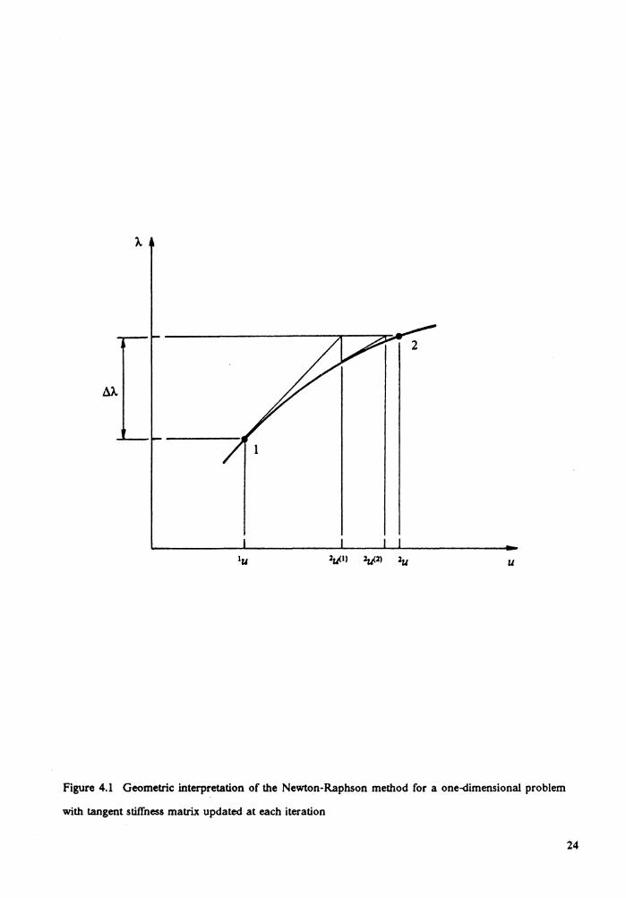
A geometrical explanation ?f the Newton-Raphson iteration is given in Fig. 4.1 for
a one-dimensional pro bl em.
23
2u(ll 2u(2) 2u u
Figure 4.1 Geometric interpretation of the Newton-Raphson method for a one-dimensional problem
with tangent stiffness matrix updated at each iteration
24
The procedure of the Newton-Raphson method is summarized as follows. For each
iteration in a fixed time step (or a load step for static analysis) the following computa-
tions are carried out:
1. Establish the system matrices 01M], J[KL], 01KNL], and'+AJ{F}(l-tl in eqn. (4.3) by using
the approximate nodal displacements, strains and stresses from the last iteration.
2. Evaluate the right-hand side of eqn. ( 4.3).
3. Solve eqn. (4.3) for {oii}<I) = {ii}<I) - {ii}<1-1>.
4. Update the nodal displacements by eqn. (4.4).
5. Test for convergence.
6. If the process has not converged, return to step 1. Otherwise go to the next time step
(or load step).
In order to reduce the amount of computations per iteration, the Newton-Raphson
method is modified by using the same system matrices O[Af], 01KL], O[KNL] for several iter-
ations. These system matrices are updated only at the begining of each time step (or load
step) or only when the convergence rate becomes poor. This modified method may re-
quire more iterations to reach a new equilibrium point.
4.3 Modified Riks/Wempner Method
As stated in Chapter 1, since the Newton-Raphson method fails to trace the response
beyond the limit point, the modified Riks/Wempner method is adopted in the present
study for the nonlinear post-buckling analysis. The theoretical development of this
25
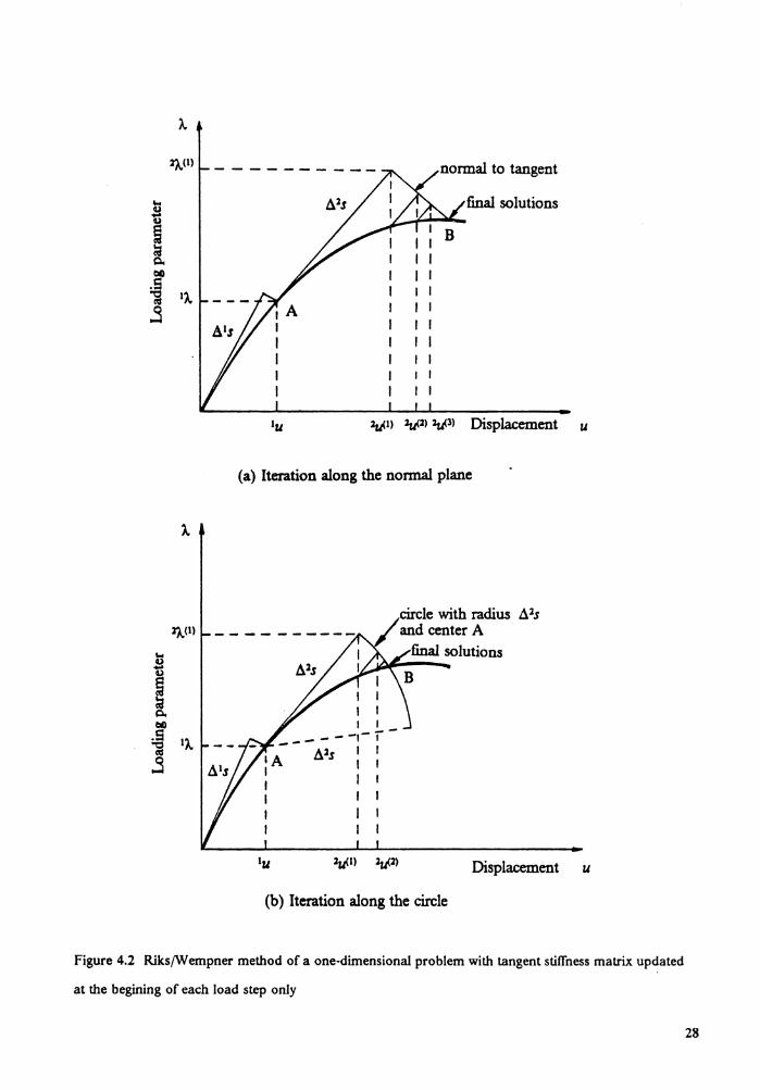
method can be found in References [44,47]. In Riks/Wempner method the load incre-
ment for each load step is considered to be an unknown and solved as part of the sol-
ution. The iteration is performed on the normal plane to the tangent of the first iteration
(or on a circle or sphere) and the new equilibrium point will be the intersection of the
normal plane (or circle, sphere) with the equilibrium path. In contrast, for Newton-
Raphson method the iterations are performed on the constant load level.
Assume that the loading is proportional, then the iterative equations corresponding
to eqn. (4.3) become (consider the static case only)
('HJ{KL] + t+&J[KNL])!t-1) {o.6,}<I)
= (t+M),,!1-1) + .6,/..(/)){Q} - IHJ{F}<t-1)
where {Q} = constant load distribution vector,
1+ 11&{Re}<1- 1> = unbalanced force vector at iteration (i-1)
= t+6t.f..(t-I) {Q} - t+dJ{F}(l-1)
1HJ{F}<t-1> = vector of nodal point forces equivalent to the element
stresses at time t + .6.t and iteration (i-1)
{ o.6,}(i) = t+M{.6,}(i) - t+M{.6,}(1-1)
= vector of increments in the nodal displacements at iteration i
.6,A,<I) = load increment
(4.5)
In order to solve N +I variables, {o.6.}<•1 and .6.A.<•1, an additional equation is used to
constrain the length of the load step
(4.6)
26
Several constraint equations have been presented such as the tangent constant arc-
length [43] and the spherical constant arc-length [44,45]. For the tangent constant arc-
length the iterations are performed on the "normal plane" while the iterations are
performed on the "sphere" for the spherical constant arc-length.
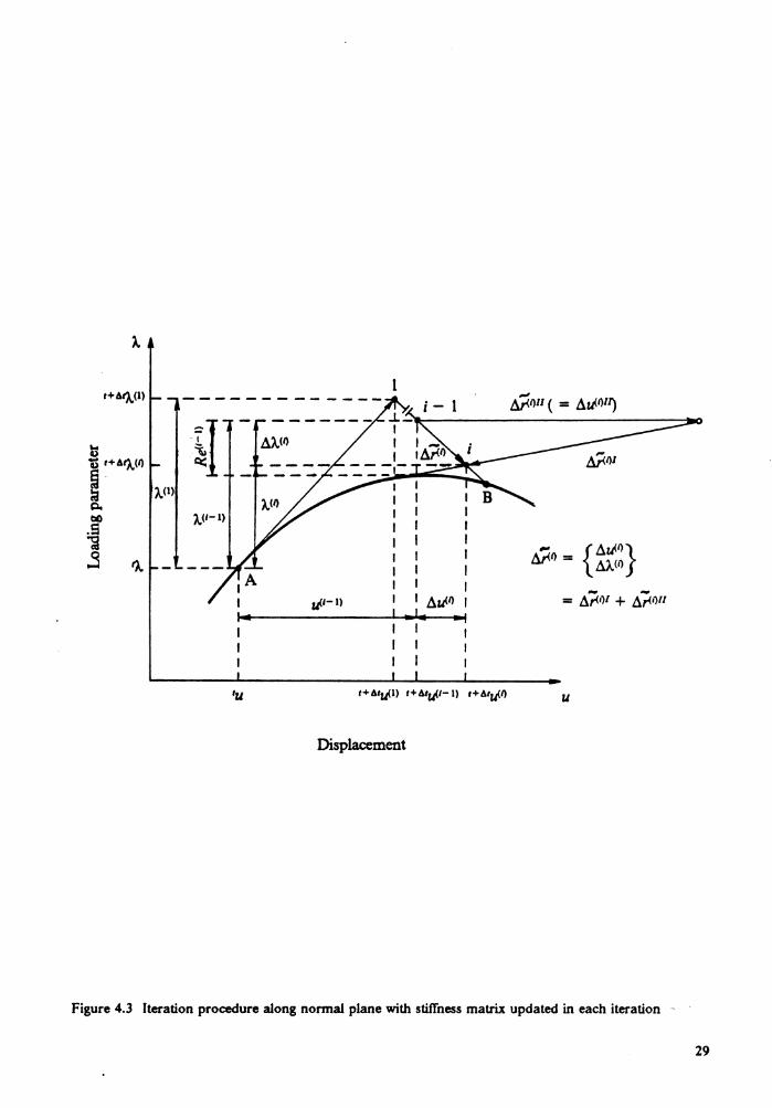
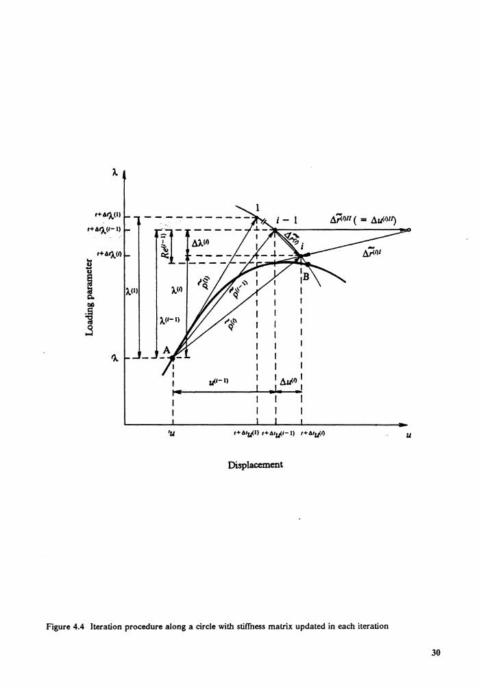
The algorithm of the modified Riks/Wempner method is briefly summarized in the
following (also see Figures 4.2, 4.3 and 4.4). The detailed theoretical development can
be found in References [43-48].
The first iteration
1. For the first load step (i.e. t= 0), choose a load increment AA.(I).
2. Calculate the system stiffness matrices J[Kd, 01KNL1 in the current configuration
3. Solve the equation
4.
(J[Kd + &[KNL]) {0A}<1>1 = {Q}
where {Q} is the constant load distribution vector.
a. For the first load step, compute the generalized arc length .1s from the con-
straint equation
As= AJ..<1>({0A}<1>1 • {oA}Clll + 1)1' 2 (by Ramm [44])
or As = AA.O> ( { oA}0>1 • { 0A}<1>1)112 (by Crisfield [45])
27
lA,(l)
lA,(l)
final solutions
2tJll 2u(l> 2t13> Displacement u
(a) Iteration along the normal plane
I I - -,-,----~s I I
I I I I I I
circle with radius ~ls and center A
final solutions
Displacement u
(b) Iteration along the circle
Figure 4.2 Riks/Wempner method of a one-dimensional problem with tangent stiffness matrix updated
at the begining of each load step only
28
fl)..<fl
'u
"'1-1)
I I I I
t+6tri-ll t+6trt.1- l) t+6t"'f)
Displacement
-~()II ( = ~uWI)
-~fl=
u
Figure 4.3 Iteration procedure along normal plane with stiffness matrix updated in each iteration -
29
t+6')..(1)
t+ 61).,(1-1) -.!. d)..(f/ a-~ - - -_ -:_-_ - - -
'u
ij.1-1)
I I I I !1£1." I
J. ·' I I I I
t+6tij.l) t+dtij.1-1) t+4tij.f/
Displacement
Figure 4.4 Iteration procedure along a circle with stiffness matrix updated in each iteration
u
30
b. For the second and higher load steps, compute the initial incremental loading
parameter dA.U> by
dA.<1> = ± ds/({od}(l)I • {od}<1>1 + 1)112 (by Ramm [44])
or dA.<1> = ± As/({0.1}<1>1 • {o.1}<1>')1!l (by Crisfield [45])
Plus indicates loading and minus indicates unloading. The sign of dA.<1> is chosen
so that the dot product of the vectors
{ {0.1}<1>1} {'{A} - 1- 41{.1}}
dA.<1> and 1 t). - t- &t).
is positive.
5. Compute the incremental nodal displacements
{ od}<1> = dA.<1> { od}<l)1
and update the total nodal displacements and the total load parameter
'+d'{d}<I> = '{d} + {oti}<l), 1+611..<11 = 'A. + AA.{l>
6. Check convergence. If convergence is achieved, go to step 14. If not, continue with
the 2nd iteration by going to step 7.
The i-th iteration, i=2, 3, ........
7. Compute the nodal force vector 1H 1{F}<1- 1> corresponds to the previous iteration
8. Update the external load vector
t+M{Q}!l-1) = t+&t).(1-1) {Q}
31
9. Update the system stiffness matrices 1+<'>J[KL]U-•> and 1+6J[KNL]<;-ii if desirable.
10. Solve for {oA}W and {oA}<•W from the two sets of equations
{J[Kd + J[KNL])U-ll {oA}W = {Q}
11. Compute the incremental load parameter At...<•1
a. If iteration on the normal plane
At...<lJ = - ( { 0A}<1>1 • { oA}W1) / ( { 0A}<1>1 0 { oA}<lJ1 + 1)
b. If iteration on the sphere, A/...<lJ is obtained from the following quadratic
equation
a (A/...<iJ)2 + 2b A/...<iJ + c = 0
where by Ramm [44]
a = {oA}W • {oA}W + 1
b = t..<1- 1> + {oA}W • ({oA}W1 + {A}<l-ll)
c = { oA}W1 • ( { oA}WI + 2{A}(l- ll)
Alternatively, by Crisfield [45]
a = { oA}W • { oA}W
b = {oA}W • ({oA}<iJ11 + {A}(l-ll)
c = ({oA}<lJll + {A}<1- 1>) • ({oA}<lJll + {A}<l-1>) - (A;)2
and A; is the arc-length of the current load step.
Two solutions A/...~'1 for this quadratic equation and two corresponding vectors
32
the improved solution corresponds to the smaller of I {orHI) I and I {orW I
12. Compute the incremental nodal displacements
{oLi}<i> = Li/..<£) {o.£i}W + {oLi}wr
and update the total nodal displacements and the total load parameter
13. Repeat steps 7 to 12 until the process has satisfied the convergence criteria.
14. Adjust the arc length for the subsequent load step by
Li; = Lis (if /)112
to control the number of future iterations, where
Lis = the arc length in the current load step, . I = no. of desired iterations ( 4 or 5 in the present study),
I = no. of iterations required in the current load step.
15. Start a new load step by returning to step 2.
4.4 Convergence Criteria
The incremental solution at the end of each iteration should be checked to see
whether it has converged within the preassigned tolerance. Here the displacement crite-
rion is adopted, i.e.
where & is the displacement convergence tolerance and is set to 0.001 in the present
study.
33
Another convergence criteria are also used, such as measuring the out-of-balance load
vector or measuring the work done by the out-of-balance loads. Some experiences with
these criteria can be found in Reference [53].
34
CHAPTER 5
ELEMENT DEVELOPMENT
5. I Introduction
In this Chapter, we develope expressions of 01Bd, &{BNd and 1HJ matrices for the de-
generated 3-D shell, degenerated 3-D curved beam, three-dimensional solid and solid-
shell transition elements, in order to find the stiffness matrices 01Kd, J[KNd and mass
matrix J[M] for those elements.
5.2 Degenerated 3-D Shell Element
Degenerated 3-D shell element is obtained by imposing two constraints on the
three-dimensional isoparametric solid element, These two con train ts are: ( 1) straight line
normal to midsurface before deformation remains straight but not normal after defor-
mation, (2) the transverse normal components of strain and hence stress are ignored in
the development. Therefore the nonlinear formulation admits arbitrarily large displace-
ments and rotations of the shell element but small strains since the thickness does not
change and the normal does not distort.
Consider the solid 3-D element shown in Fig. 5.1. Let~. 11 be the curvilinear coordi-
nates in the middle surface of the shell and ' be the coordinate in the thickness direction.
Here~. 11 and~ are normalized such that they vary between -1 and + 1. The coordinates
of a typical point in the element can be written as
(5. 1)
35
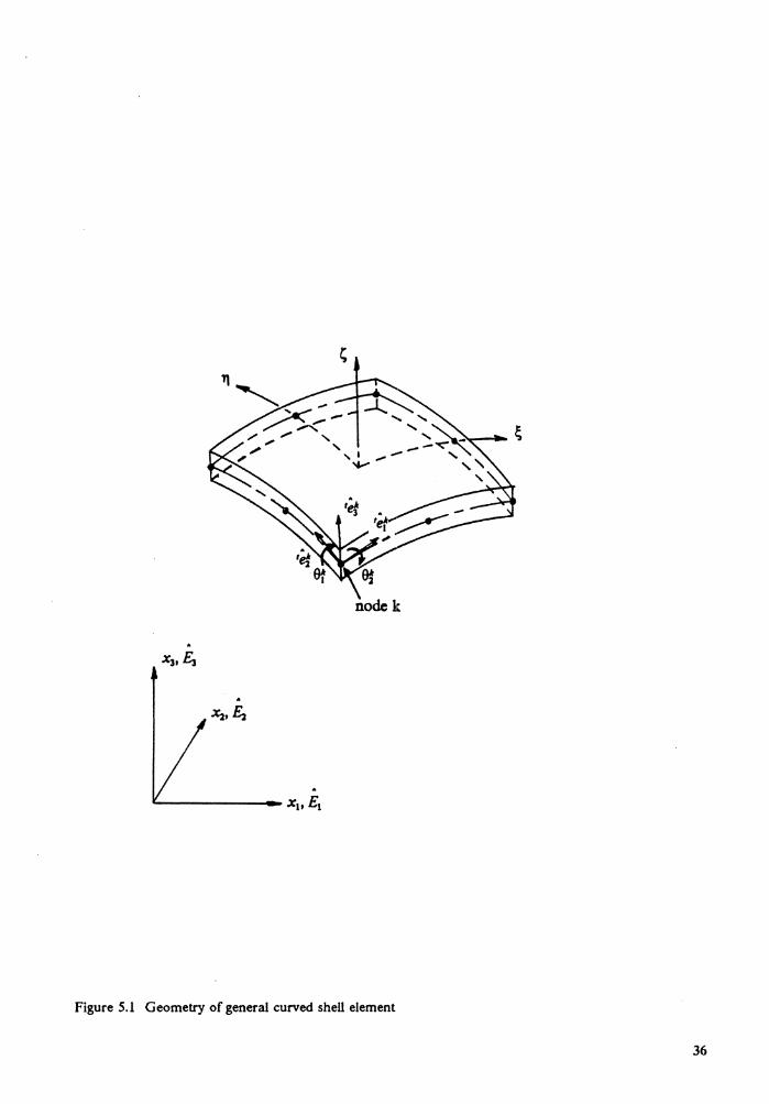
nodek
Figure 5.1 Geometry of general curved shell element
36
where n is the number of nodes in the element, and <pk(~. 11) is the finite element in-
terpolation function associated with node k. If <pk(~. 11) are derived as interpolation
functions of a parent element, square or triangular in plane, then compatibility is
achieved at the interfaces of curved space shell elements. Define
-
V1'1 = (.xf)top - (xf )bottom
e~,=vulv~I
where V1 is the vector connecting the upper and lower points of the normal at node k.
Eqn. (5.1) can be rewritten as
(5.2)
where hk = I ii; I is the thickness of the shell element at node k. Hence, the coordinates
of any point in the element at time t are interpolated by the expression
(5.3)
and the displacements by
Here 1uf and ut denote, respectively, the displacement and incremental displacement
components in the x, -direction at the k-th node and time t. For small rotation dQ at
each node
du = e~ 'et + et 'e~ + e~ 'e~
the increment of vector 1e~ can be written as
37
(5.6)
Then eqn. (5.5) becomes
i = 1, 2, 3 (5.7)
The unit vectors 'ef and 'e~ at node k can be obtained from the relations
~ x 'e: I~ x 'e:I
(5.8)
. where E, are the unit vectors of the stationary global coordinate system. Eqn. (5.7) can
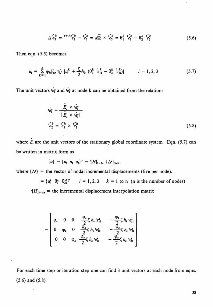
be written in matrix form as
where {~·} = the vector of nodal incremental displacements (five per node).
= {ut 0f 0~}T i = 1, 2, 3 k = 1 to n (n is the number of nodes)
1H13 xsn = the incremental displacement interpolation matrix
<pk 0 0 ~h tk 2 k eu ~h tk - 2 k e21
= 0 <pk 0 ~h tk 2 k e12 - ~h 'ek 2 k 22
0 0 'Pk ~h tk 2 k €13 ~h tk - 2 k €23
For each time step or iteration step one can find 3 unit vectors at each node from eqns.
(5.6) and (5.8).
38
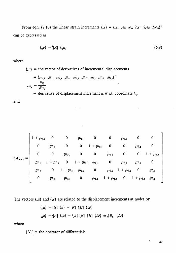
can be expressed as
where
{oe} = 1[A] {ou}
{ 0u} = the vector of derivatives of incremental displacements
= {0U1,1 0U1; 0U1,3 o~.1 oUl,2 0~,3 oU3,l oU3,2 oU3,3} T
OU1 0U1J = -;Q u x1
= derivative of displacement increment u1 w.r.t. coordinate 0x1
and
1 + JU1,1 0 0 J~.l 0 0 JU3,1 0
0 JU1,2 0 0 1 + J~,2 0 0 Ju3.l
0 0 Ju1.J 0 0 J"2_3 0 0 1A]6x9 =
JU1,2 l + Ju1.1 0 l + J~,2 d"2.1 0 Ju3.2 ifU3,1
JU1.3 0 1 + JU1,1 J~.3 0 ri"2.1 I + JU3,3 0
0 JU1.3 Ju1.2 0 J~.3 I +.:~ 0 I + JU3,3
(5.9)
0
0
l + Ju3,3
0
JU3,1
Ju3.2
The vectors {0u} and {0e} are related to the displacement increments at nodes by
{ 0u} = [N] {u} = [N] 1H] {~·}
{oe} = 1A] {ou} = 1[A] [N] 1H] {~·} = ti[BL] {~·}
where
[N]r = the operator of differentials
39
o o o 0 0 0 0 0 0 ------o0x, o0xl o0x3
= 0 0 0 o o o 0 0 0 ------aox, o0x2 D°X3
0 0 0 0 0 0 o o o ------ooxl aox2 OOX3
and O{Bd = 1[A] [N] 1H] = the linear incremental strain-displacement matrix.
The components of 1[A] contains Ju,J. From eqn. (5.4) the global displacements are
related to the natural curvilinear coordinates ~. 11 and linear coordinate '· Hence the
derivatives of these displacements Ju,J with respect to the global coordinates
0x" 0x2 and 0x3 are obtained by a matrix relation
olul OIU2 OIU3 olul OIU2 OIU3 0 0 X1 aoxl 0 0 X1 o~ o~ o~
[~u1J] = OIU1 atu2 OIU3 = o[J]-1 OIU1 O(U2 O(U3
(5.10) 0 0 0 o11 011 " 0 X2 0 X2 0 X2 011
OIU1 OIU2 O(U3 atul o'u2 a'u3 0 0 X3 0 0 X3 OOX3 o' o' a'
The J ocobian matrix 0[1] is defined as
0 0 X1 0 0 X2 0 0 X3 a~ o~ a~ 0 0 0
o[J] = 0 X1 0 X2 0 X3 ( 5.11) 011 011 011 0 0 X1 0 0 X2 aox3 o' o' a,
40
and is computed from the coordinate definition of eqn. (5.3). The derivatives of dis-
placements ru1 with respect to the coordinates ~. TJ and ~ can be computed from eqn.
(5.4).
In the evalutions of element matrices in eqns. (3.4) to (3. 7), the integrands, (i.e.
&[BL] , 0[ C] , &[BNL] , &[SJ , t[H] and J{S} ) should be expressed in the same
coordinate system, namely the global coordinate system (0x1 , 0x2 , 0x3) or the local
curvilinear system (x'1 , x'2 , x'3) which is aligned with the shell element midsurface. In
this study we express the matrices and vector of the integrands in the local coordinate
The ~umber of stress and strain components are reduced to five since we neglect the
transverse normal components of stress and strain. Hence, the global derivatives of
displacements, [Ju1J] which are obtained in eqn. (5.10), are transformed to the local de-
rivatives of the local displacements along the orthogonal coordinates by the following
relation (also see Ref. [ 11])
a' , U I a' I U2 a' , U3 ax'1 ax'1 ax'1 a'u'1 a' I at I U2 U3
[8Jf x 3 [~ulJ] [8]3 x 3 (5.12) = ax'2 ax'2 ax'2 a' I U I a' I U2 a' , U3 ax13 ax13 ax13
where [0]T is the transformation matrix between the local coordinate system
(x'1 , x'2 , x'3) at the integration point and the global coordinate system (0x1 , 0x2 , 0x3).
The transformation matrix [0] is obtained by intepolating the three orthogonal unit
vectors (t~1 , 1~2 , '~3) at each node
41
n n n
L <pk tef1 k-1 L <pk te11 k-1 L <pk te§1 k-1
n n n
[SJ= L <pk tef:z L <J> rek L <pk te§2 k-1 k-1 k 22 k-1
n n n
:E <pk ref3 k-1 L <pk 'e13 k-1 L <pk te§3 k-1
Since the element matrices are evaluated using numerical integration, the transformation
must be performed at each integration point during the numerical integration.
In order to obtain &[BL], the vector of derivatives of incremental displacements
{ Uo} needs to be evaluated. Equations ( 5.10) and ( 5.12) can be used again except that
ru, are replaced by u, and the interpolation equation for u,, eqn. (5.5), is applied.
The constitutive relation, 0[ C'], for the k-th lamina of a laminated composite shell
in the local coordinate system (x'1 , x'2 , x'3) can be expressed as
C'11 C' 12 C'13 0 0
C' 12 C'22 C'23 0 0
o[ C'](k) = C'13 C'23 C'33 0 0 (5.13)
0 0 0 C'44 C'45
0 0 0 C'45 C'ss
where
C'12 = m 2n2 (Qu + Q22 - 4Q33) + (m4 + n4)Q12
C'13 = mn[m2 Q11 - n2 Q:u - (m2 - n2)(Q12 + 2Q33)]
42
C'22 = n4 Qu + 2m2n2 (Q12 + 2Q33) + m4 Q22
C'23 = mn[n2 Qu - m2 Q22 + (m2 - n2)(Q12 + 2Q33)]
C'33 = m2n2 (Qu + Q22 - 2Q,2) + (m2 - n2)2 QJJ
m = cos e(k) ' n = sin e(k)
Q,1, which are the plane stress-reduced stiffnesses of an orthotropic lamina in the material
coordinate system, are reduced from the constitutive relations for three-dimensional
orthotropic body by neglecting the normal stress in the thickness direction. The Qij can
be expressed in terms of engineering constants of a lamina
' Q22 = 1
(5.14)
where" AK" is the shear correction coefficient which is taken to be equal to 5/6.
To evaluate element matrices in eqns. (3.4) - (3.7), we employ the Gaussian
quadrature to perform the integrations. Since we are dealing with laminated composite
structures, the integration through the thickness involves individual lamina. One way is
to use Gaussian quadrature through the thickness direction. Since the constitutive re-
latio.n 0[ C] is different from layer to layer and is not a continuous function in the
thickness direction, the integration should be performed separately for each layer (see
[14,54]). This increases the computation time as the number of layers is increased. An
alternative way is to perform explicit integration through the thickness and reduce the
problem to a 2-D one. The Jacobian matrix, in general, is a function of~' 11 and'· The
43
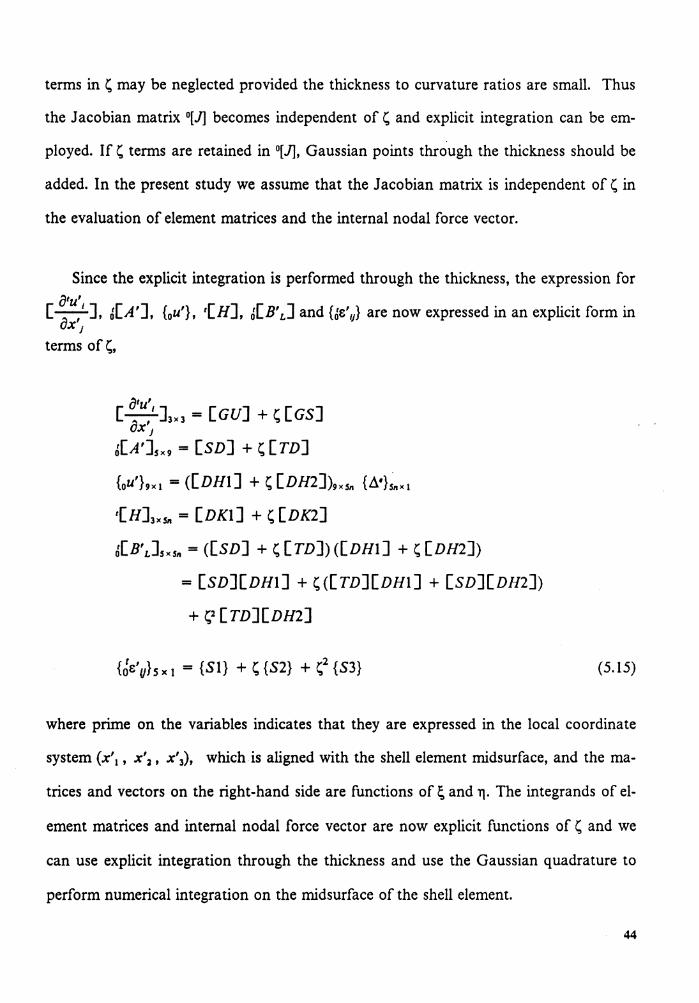
terms in ~ may be neglected provided the thickness to curvature ratios are small. Thus
the Jacobian matrix 0[J] becomes independent of~ and explicit integration can be em-
ployed. If~ terms are retained in °[1], Gaussian points through the thickness should be
added. In the present study we assume that the Jacobian matrix is independent of~ in
the evaluation of element matrices and the internal nodal force vector.
Since the explicit integration is performed through the thickness, the expression for o' , [~], J[A'], {0u'}, {HJ, J[B'L] and {Je',1} are now expressed in an explicit form in ox' I terms of~,
o' , [~]3x3 =[GU]+~ [GS] ox' I J[A'Jsx9 = [SD] +~[TD]
{ou'}9x1 = ([DHl] + ~ [DH2])9x5n {~'}snxl
{H]3x5n = [DKl] + ~ [DK2]
J[B'LJsxsn =([SD] + ~ [TD])([DHl] + ~ [DH2])
= [SD][DHl] + ~([TD][DHl] + [SD][DH2])
+ ~2 [TD][DH2]
{cie'y}sxt = {Sl} + ~{S2} + ~2 {S3} (5.15)
where prime on the variables indicates that they are expressed in the local coordinate
system (x'1 , x'2 , x'3), which is aligned with the shell element midsurface, and the ma-
trices and vectors on the right-hand side are functions of~ and 11· The integrands of el-
ement matrices and internal nodal force vector are now explicit functions of ~ and we
can use explicit integration through the thickness and use the Gaussian quadrature to
perform numerical integration on the midsurface of the shell element.
44
For thin shell structures, in order to avoid 'element locking' we use reduced inte-
gration scheme to evaluate the stiffness coefficients associated with the transverse shear
deformation. Hence we split the constitutive matrix 0[ C'] into two parts, one without
transverse shear moduli 0[ C'] 8, and the other with only transverse shear moduli
0[ C']5 • Full integration is used to evaluate the stiffness coefficients containing 0[ C'] 8 ,
and reduced integration is used for those containing 0[ C' ] 5 •
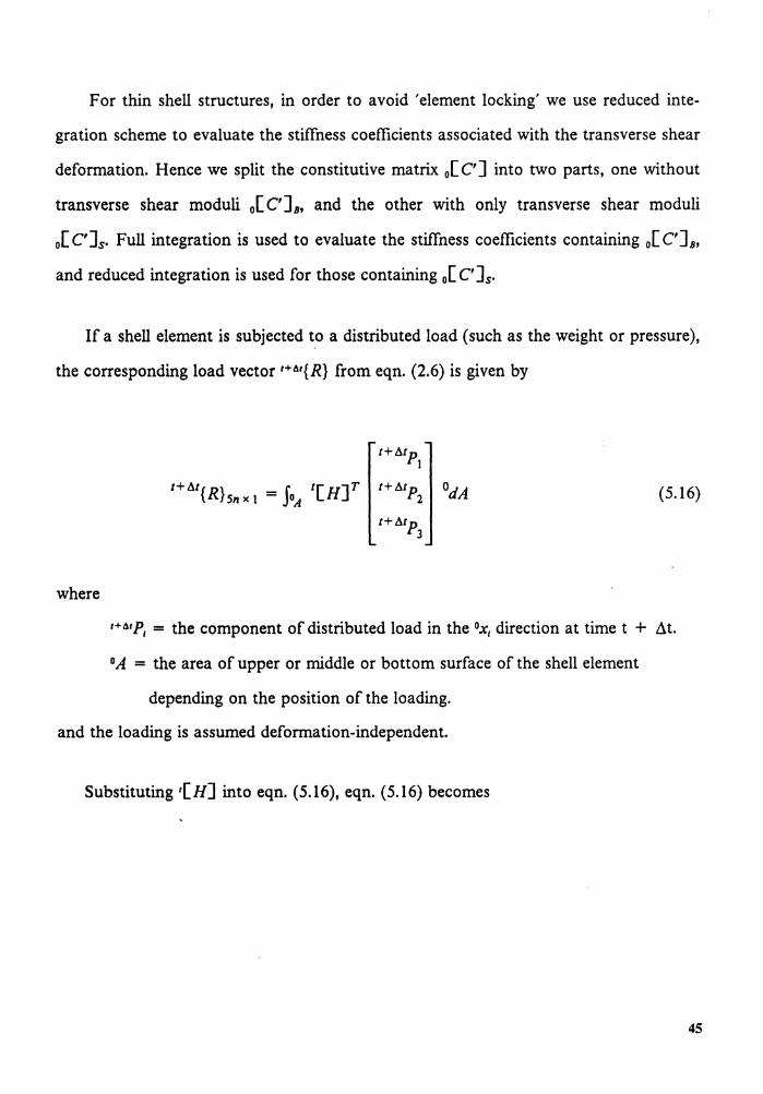
If a shell element is subjected to a distributed load (such as the weight or pressure),
the corresponding load vector t+&t{R} from eqn. (2.6) is given by
t+Mp1
t+M{R}sn x I = JoA '[H]T t+!J.tp2 odA
t+!J.tp3
(5.16)
where
t+&rp, = the component of distributed load in the 0x, direction at time t + .1.t.
0 A = the area of upper or middle or bottom surface of the shell element
depending on the position of the loading.
and the loading is assumed deformation-independent.
Substituting t[ H] into eqn. ( 5.16), eqn. ( 5.16) becomes
45
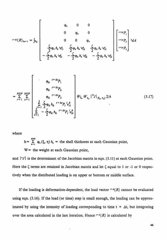
<pk 0 0
0 <pk 0 t+lltpl
r+ilt{R} - } Snxl - O,c 0 0 <pk t+lltpl
f<pk hk 1ef1 f<pk hk 1et2 f<pk hk 1ef3 t+t.tpl
- .£<p h 'ek 2 k k 21 - f<pkhk 'et - .£<p h 'ek 2 k k 23
NGP NGP = l: l:
r= 1 :r= 1
where NPE
h = l: <pk{~, 11) hk = the shell thickness at each Gaussian point, k-1 W = the weight at each Gaussian point,
0dA
(5.17)
and I 0JI is the determinant of the Jacobian matrix in eqn. (5.11) at each Gaussian point.
Here the~ terms are retained in Jacobian matrix and let~ equal to 1 or -1 or 0 respec-
tively when the distributed loading is on upper or bottom or middle surface.
If the loading is deformation-dependent, the load vector i+il{R} cannot be evaluated
using eqn. (5.16). If the load (or time) step is small enough, the loading can be approx-
imated by using the intensity of loading corresponding to time t + ~t, but integrating
over the area calculated in the last iteration. Hence i+ll{R} is calculated by
46
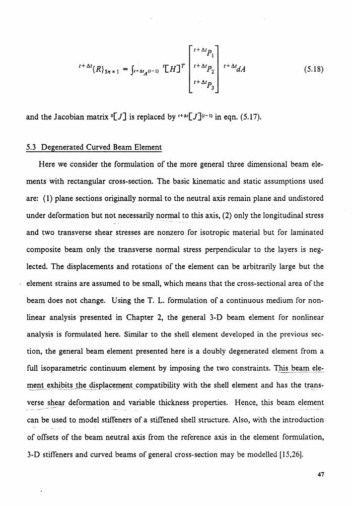
t+ Mp 1
t+M{R}sn x 1 = Ji+MA(l-1) '[H]T t+Mp2 t+MdA
t+Mp3
and the Jacobian matrix 0[J] is replaced by 1H'[J]<1-1> in eq n. ( 5.17).
5.3 Degenerated Curved Beam Element
(5.18)
Here we consider the formulation of the more general three dimensional beam ele-
ments with rectangular cross-section. The basic kinematic and static assumptions used
are: ( 1) plane sections originally normal to the neutral axis remain plane and undistored
under deformation but not necessarily normal to this axis, (2) only the longitudinal stress -· . ----- - --
and two transverse shear stresses are nonzero for isotropic material but for laminated
composite beam only the transverse normal stress perpendicular to the layers is neg-
lected. The displacements and rotations of the element can be arbitrarily large but the
element strains are assumed to be small, which means that the cross-sectional area of the
beam does not change. Using the T. L. formulation of a continuous medium for non-
linear analysis presented in Chapter 2, the general 3-D beam element for nonlinear
analysis is formulated here. Similar to the shell element developed in the previous sec-
tion, the general beam element presented here is a doubly degenerated element from a
full isoparametric continuum element by imposing the two constraints. rhis b~aI!l __ ~J~_-
J:!!en_!_~~E-~!~ _ _!P,_~_<!!sp_l(i_C~!Il~I1t_~c:>I1:1Pc:\tibility with the shell element and has .the tra.ns-
verse shea.r. deformation and variable thickness properties. Hence, this beam element - .----··-·' -·- -·-·-- .
can be used to model stiffeners of a stiffened shell structure. Also, with the introduction
of offsets of the beam neutral axis from the reference axis in the element formulation,
3-D stiffeners and curved beams of general cross-section may be modelled [15,26].
47
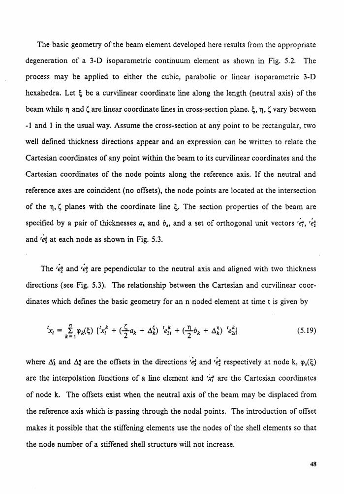
The basic geometry of the beam element developed here results from the appropriate
degeneration of a 3-D isoparametric continuum element as shown in Fig. 5.2. The
process may be applied to either the cubic, parabolic or linear isoparametric 3-D
hexahedra. Let ; be a curvilinear coordinate line along the length (neutral axis) of the
beam while 11 and~ are linear coordinate lines in cross-section plane. ~. 11, ~vary between
-1 and 1 in the usual way. Assume the cross-section at any point to be rectangular, two
well defined thickness directions appear and an expression can be written to relate the
Cartesian coordinates of any point within the beam to its curvilinear coordinates and the
Cartesian coordinates of the node points along the reference axis. If the neutral and
reference axes are coincident (no offsets), the node points are located at the intersection
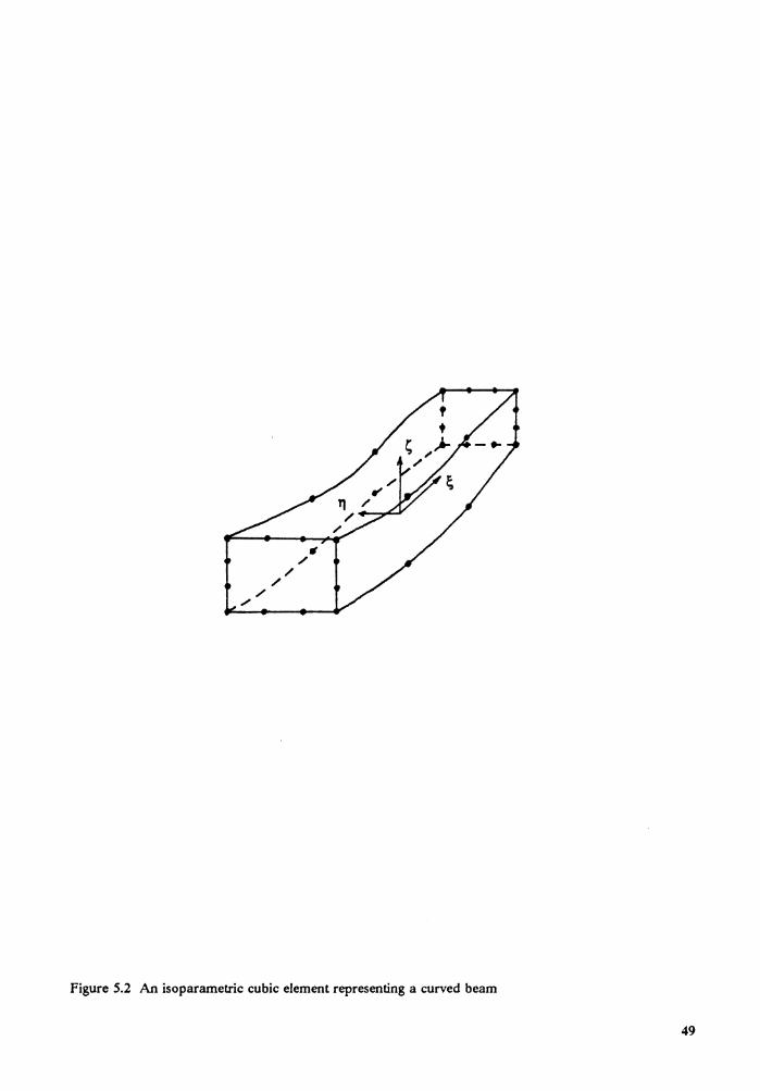
of the 11, ~ planes with the coordinate line ~· The section properties of the beam are
specified by a pair of thicknesses ak and bk, and a set of orthogonal unit vectors 1ef, 1e1
and 1e~ at each node as shown in Fig. 5.3.
The 1e~ and 1e~ are pependicular to the neutral axis and aligned with two thickness
directions (see Fig. 5.3). The relationship between the Cartesian and curvilinear coor-
dinates which defines the basic geometry for an n noded element at time t is given by
(5.19)
where .!ii and Li~ are the offsets in the directions 1e~ and 1e~ respectively at node k, q>k(~)
are the interpolation functions of a line element and 1,Xf are the Cartesian coordinates
of node k. The offsets exist when the neutral axis of the beam may be displaced from
the reference axis which is passing through the nodal points. The introduction of offset
makes it possible that the stiffening elements use the nodes of the shell elements so that
the node number of a stiffened shell structure will not increase.
48
/ /
/
/ • /
Figure 5.2 An isoparametric cubic element representing a curved beam
49
Coordinate system at node 1
1
(~J and ~i are the offsets)
Figure 5.3 Geometry of a parabolic curved beam element
At time t
Neutral
2
50
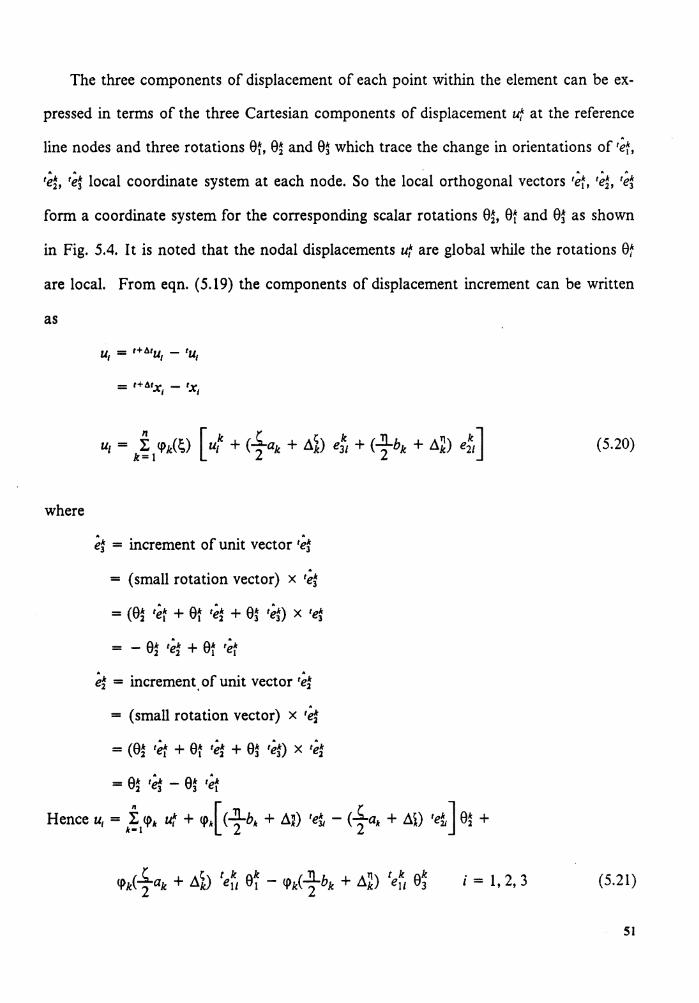
The three components of displacement of each point within the element can be ex-
pressed in terms of the three Cartesian components of displacement uf at the reference
line nodes and three rotations 0f, e~ and e~ which trace the change in orientations of 'ef,
1e~, 1e~ local coordinate system at each node. So the local orthogonal vectors 'ef, 1e~, 'e~
form a coordinate system for the corresponding scalar rotations 0~, 0f and 0~ as shown
in Fig. 5.4. It is noted that the nodal displacements uf are global while the rotations 0f
are local. From eqn. (5.19) the components of displacement increment can be written
as
u, = t+t.1u1 - 1u1
= 1+ t.tx1 - 1x1
" [ k ~ ~ k ....!l.. ,, k] u, = k~ 1 cpi;) u, + ( 2 ak + Lik) e31 + ( 2 bk + Lik) e11 (5.20)
where
e: = increment of unit vector 1e: = (small rotation vector) x 1e: = (e~ 'et + er 'e~ + e~ 'eD x 'e: - - ek 'e·k + 0" 'e·" - 2 2 I I
e~ = increment' of unit vector 'e~
= (small rotation vector) x 1e~
= (0~ 'et + 0f 'e~ + e~ 'e:) x 'e~
= e~ 1e: - e~ 'et Hence u, = k~1 q>k uf + q>"[ (Tb" + Li~) 'et - <fak + Lil) 'et J 0i +
q>k(fak + Lik) te~, et - cpi-}bk + Lii) te~, e~ j = l, 2, 3 (5.21)
51
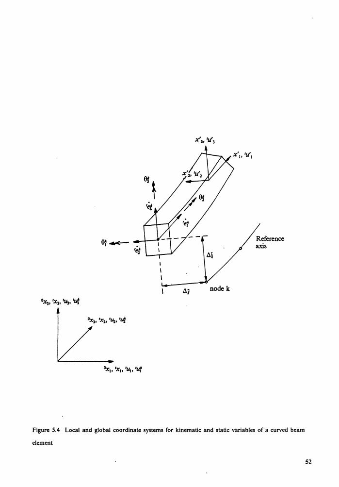
I I I
node k
Figure 5.4 Local and global coordinate systems for kinematic and static variables of a curved beam
element
52
From this expression the incremental displacement interpolation matrix 1H] for the
beam element can be formulated as:
q>k 0 0 q>kfak + .11)'ef1 <i>1r[(-}bk + .1~)te~1 - (fa1r + .10 1e11J
0 <f>1r 0 <i>1r(fak + .10 'ef:i <j>1r[(fbk + .1:)1e~2 - (fa.1: + .10 1et]
0 0 <f>1r q>k(fa.1: + .10 1ef3 <i>1r[(fb1r + .1~) 1e~3 - (fa1r + .10 'et]
(5.22)
- <i>i -}b1r + .1~)'ef,
- <i>1r(fb1r + .1~)'ef2
- <i>1r(fb1r + .1~)'ef3
Using eqns. (3.4) to (3.7) and this 1HJ for beam element, the beam element matrices
and internal force vector needed in the eqn. (4.3) can be obtained. The processes to
evaluate element matrices and internal force vector are the same as that for the shell el-
ement in the last section. The main difference is that in carrying out the numerical inte-
gration of element matrices, we perform explicit intergration through the two thickness
directions and reduce the problem to a 1-D one. The Jacobian matrix 0[1] becomes in-
dependent of 11 and~ if we neglect the terms in 11 and~' and then explicit integration can
be employed to evaluate the element matrices and the internal nodal force vector.
Since the explicit integration is performed through two thickness directions, 11 and ~. i)tu'
the expressions for[--'], J[A'], {0u'}, t[H], J[B'L] and {Je'IJ} are now expressed in ox'1
an explicit form of 11 and~' i.e.
i)tu' [-' ]3x3 =[GU] +~[GS] + 11 [GQ]
ox'1 J[A'Jsx9 = [SD] +~[TD] + 11 [UD]
{ou'}9x1 = ([DHl] + ~ [DH2] + 11 [DH3])9x6n {.1•}6nxl
53
{H]3 x6n = [DKI] + ~ [DK2] + 11 [DK3]
J[B'LJsx6n =([SD] +~[TD] + 11 [UD])([DHI] + ~ [DH2] + 11[DH3])
= [SD][DHI] + ~([TD][DHI] + [SD][DH2])
+ ~2 [TD][DH2] + 11([UD][DHI] + [SD][DH3])
+ 112 [UD][DH3] + 11~([UD][DH2] + [TD][DH3])
{J&'lj}sx1 = {SI} + ~ {S2} + ~2 {S3} + 11 {S4} + ~11 {S5} + 112 {S6}
where prime indicates that the quantities are expressed in the local coordinate system
(x' 1 , x'2 , x'3), which is aligned with the neutral axis of the beam element, and the
matrices and vectors on the right-hand side are functions of ~ only. The integrands of
element matrices and internal nodal force vector are now explicit functions of 11 and ~·
Therefore explicit integration is employed through the two thickness directions, and the
Gaussian quadrature is used to perform numerical integration in the longitudinal direc-
tion. The reduced/selective integration scheme is used to avoid "element locking".
For laminated composite beam the same constitutive relations as that for laminated
composite shell is used and five components of stress and strain are retained.
The external force vector 1+41{R} for a beam element subjected to distributed line load
is evaluated by letting 11 = 0, then similar to eqn. (2.6) we have
where
t+Mp1
t+M{R}6n x I = JoL t[H]T t+Mp2 I odL t+Mp3
(5.23)
t+Mp1 = the component of distributed load in the 0x; direction at time t + Lit.
0 L = the length of line which is the intersection of 11 = 0 plane with
54
upper or lower surface of the beam.
and the loading is assumed deformation-independent.
Substituting t[H] from eqn. (5.22) into eqn. (5.23), we obtain
t+ t:.t{R} 6n x 1
NGP = l:
r= 1 W;, I 011;,4/(ab) (5.24)
where NPE
a = l: q>* {~, 11) a* = the beam thickness in ~ direction at each Gaussian point, k-1 NPE
b = l: q>1r (~, 11) bk = the beam thickness in 11 direction at each Gaussian point, k-1
W = the weight at each Gaussian point,
and 1°11 is the determinant of the Jacobian matrix at each Gaussian point. Here the
11 and~ terms are retained in Jacobian matrix and let 11 = 0 and ' = 1 or -1 or 0 re-
spectively when the distributed line loading is on upper or bottom or middle surface. If
the loading is deformation-dependent, similar modifications as discussed for shell ele-
ment should be made.
In analyzing stiffened plate or shell, the external load vector is evaluated for shell
elements only by using eqn. (5.17) and we do not compute eqn. (5.24) since the stiffener
elements have common nodes with the shell elements.
55
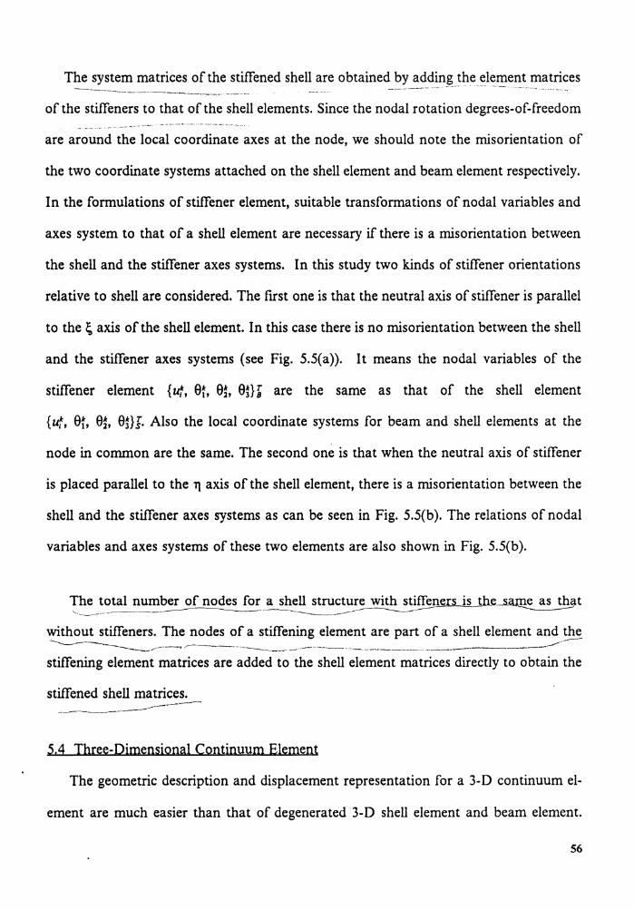
The system matrices of the stiffened shell are obtained by adding ~he ~l~f!lent matrices ----- ----~----- --- ---
of the stiffeners to that of the shell elements. Since the nodal rotation degrees-of-freedom
are around the local coordinate axes at the node, we should note the misorientation of
the two coordinate systems attached on the shell element and beam element respectively.
In the formulations of stiffener element, suitable transformations of nodal variables and
axes system to that of a shell element are necessary if there is a misorientation between
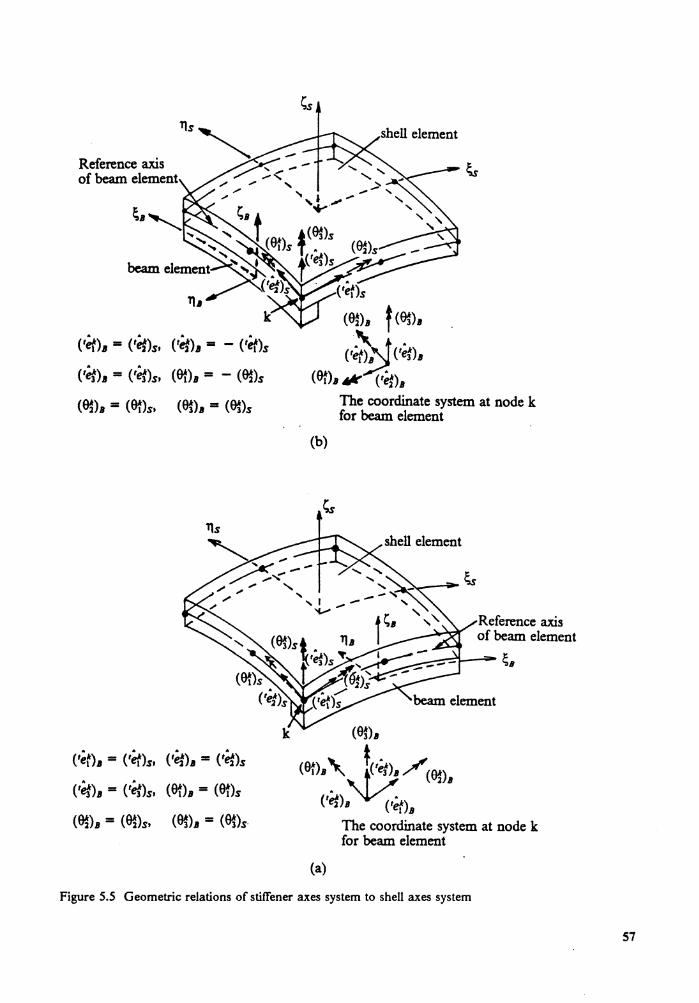
the shell and the stiffener axes systems. In this study two kinds of stiffener orientations
relative to shell are considered. The first one is that the neutral axis of stiffener is parallel
to the~ axis of the shell element. In this case there is no misorientation between the shell
and the stiffener axes systems (see Fig. 5.5(a)). It means the nodal variables of the
stiffener element {uf, St, S~, S~H are the same as that of the shell element
{uf, St, S~, SDI· Also the local coordinate systems for beam and shell elements at the
node in common are the same. The second one is that when the neutral axis of stiffener
is placed parallel to the 11 axis of the shell element, there is a misorientation between the
shell and the stiffener axes systems as can be seen in Fig. 5.5(b ). The relations of nodal
variables and axes systems of these two elements are also shown in Fig. 5.S(b ).
The total number of nodes for a shell structure with st~e_s.~t '--~----~---------------------------------------
without stiffeners. The nodes of a stiffening element are part of a shell element and th~ _______________ .- ___ ___,,-------------------~--------------------------~-------~---------~----_.,,.,-----
stiffening element matrices are added to the shell element matrices directly to obtain the
stiffened shell matrices. ~----------------
5.4 Three-Dimensional Continuum Element
The geometric description and displacement representation for a 3-D continuum el-
ement are much easier than that of degenerated 3-D shell element and beam element.
56
Reference axis of beam element
('~)., = ('tf)s, ('tf)., = - ('~)s
('et)., == ('tt)s, (0t)., == - (~)s
(~)., == (0t)s, (~)., == (~)s
('et)., == ('~)s, ('~). == ('tf)s
('tf). == ('tt)s, (E}t)., == (0t)s
(~)s == (~)s, (~)., = (~)s·
~s
(b)
~
~
The coordinate system at node k for beam element
~
--------- ~.
it - can. (01),:~/(0!).
('e!h ('~).
(a)
The coordinate system at node k for beam element
Figure 5.5 Geometric relations of stiffener axes system to shell axes system
57
The relationship between the Cartesian and curvilinear coordinates for an n node ele-
ment at time t is given by
(5.26)
The displacements at time t is 1u1 = 1x1 - 0x,. Hence, the incremental displacements from
time t to t + tit are obtained as
(5.27)
It is noted that now there are only 3 d.o.f. at each node, i.e. three incremental translation
displacements. From eqn. (5.27) the incremental displacement interpolation matrix '[H]
for the 3-D continuum element can be formulated as follows:
q>k 0 0
t[H]3 x Jn = 0 <9k 0
0 0 <9k
(5.28)
Using eqns. (3.4) to (3.7) again and 111] in eqn. (5.28), the element matrices and
internal nodal force vector for 3-D continuum element can be obtained. The procedure
is similar to that in the previous sections for shell and beam elements, except that no
kinematic and static assumptions are imposed. Hence there are six components for
stresses and strains respectively in local coordinate system (x' 1 , x'2 , x\) aligned with
the element. That is
{ '} { ' ' ' .., ' .., ' .., ' } T oe 6 x 1 = oe 11 oe 22 oe 33 "-Oe 23 "-Oe 13 "-Oe 12
58
(5.29)
Also the transformation matrix [0] at each integration point is formulated in a different
way. Here [0] is given by
(5.30)
where
O'x1 O'X1 a~ a,, -... O'X2 o'X2 QJ Q3 == x qJ =---a~ a,, IQJI 01X3 iJtx3
a1; a,,
The constitutive matrix 0[ C']1k1 for the k-th lamina oflaminated composite structure
in the local coordinate system (x'1 , x'2 , x'3) can be expressed as
59
where
C' 11 C'12 C'13 0 0
C'12 C'22 C'23 0 0
C'13 C'23 C'33 0 0 o[ C'](k) =
0 0 0 C'44 C'45
0 0 0 C'45 C'ss
C'16 C'26 C'36 0 0
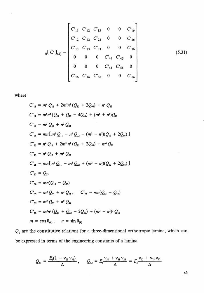
C'u = m4 Qu + 2m2n2 (Q12 + 2Q66) + n4 Q2l
C'12 = m2n2 (Qu + Q2l - 4Q66) + (m4 + n4)Q12
C'33 = Q33
m = cos e(k)' n = sin e(k)
C'16
C'26
C'36 (5.31)
0
0
C'66
Q;1 are the constitutive relations for a three-dimensional orthotropic lamina, which can
be expressed in terms of the engineering constants of a lamina
60
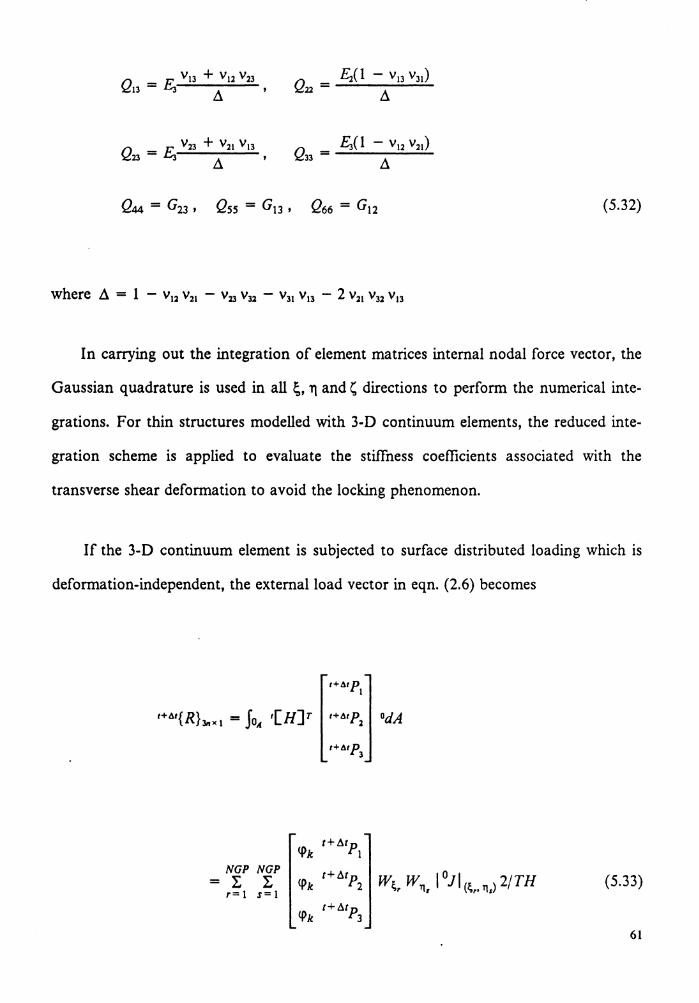
(5.32)
In carrying out the integration of element matrices internal nodal force vector, the
Gaussian quadrature is used in all ~. 11 and' directions to perform the numerical inte-
grations. For thin structures modelled with 3-D continuum elements, the reduced inte-
gration scheme is applied to evaluate the stiffness coefficients associated with the
transverse shear deformation to avoid the locking phenomenon.
If the 3-D continuum element is subjected to surface distributed loading which is
deformation-independent, the external load vector in eqn. (2.6) becomes
<pk t+tJ.tp
I NGP NGP t+Mp2 w~, w11 , I 011 (~,. ri,) 2/TH = l: l: <pk (5.33) r=I s=I
<pk t+Mp3
61
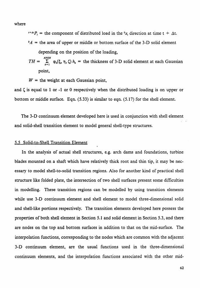
where
t+MP1 = the component of distributed load in the 0x, direction at time t + ~t. 0A = the area of upper or middle or bottom surface of the 3-D solid element
depending on the position of the loading, NPEH
TH = l; q>i~, T}, ~) h11: = the thickness of 3-D solid element at each Gaussian 11:•1
point,
W = the weight at each Gaussian point,
and ~ is equal to 1 or -1 or 0 respectively when the distributed loading is on upper or
bottom or middle surface. Eqn. (5.33) is similar to eqn. (5.17) for the shell element.
The 3-D continuum element developed here is used in conjunction with shell element
and solid-shell transition element to model general shell-type structures.
5.5 Solid-to-Shell Transition Element
In the analysis of actual shell structures, e.g. arch dams and foundations, turbine
blades mounted on a shaft which have relatively thick root and thin tip, it may be nee-
essary to model shell-to-solid transition regions. Also for another kind of practical shell
structure like folded plate, the intersection of two shell surfaces present some difficulties
in modelling. These transition regions can be modelled by using transition elements
while use 3-D continuum element and shell element to model three-dimensional solid
and shell-like portions respectively. The transition elements developed here possess the
properties of both shell element in Section 5.1 and solid element in Section 5.3, and there
are nodes on the top and bottom surfaces in addition to that on the mid-surface. The
interpolation functions, corresponding to the nodes which are common with the adjacent
3-D continuum element, are the usual functions used in the three-dimensional
continuum elements, and the interpolation functions associated with the other mid-
62
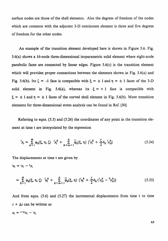
surface nodes are those of the shell elements. Also the degrees of freedom of the nodes
which are common with the adjacent 3-D continuum element is three and five degrees
of freedom for the other nodes.
An example of the transition element developed here is shown in Figure 5.6. Fig.
5.6(a) shows a 16-node three-dimensional isoparametric solid element where eight-node
parabolic faces are connected by linear edges. Figure 5.6( c) is the transition element
which will provides proper connections between the elements shown in Fig. 5.6(a) and
Fig. 5.6(b). Its ~ = -1 face is compatible with ~ = ± 1and11 = ± l faces of the 3-D
solid element in Fig. 5.6(a), whereas its ~ = + l face is compatible with
~ = ± 1 and 11 = ± I faces of the curved shell element in Fig. 5.6(b ). More transition
elements for three-dimensional stress analysis can be found in Ref. [50].
Referring to eqns. (5.3) and (5.26) the coordinates of any point in the transition ele-
ment at time t are interpolated by the expression
(5.34)
The displacements at time t are given by
(5.35)
And from eqns. (5.6) and (5.27) the incremental displacements from time t to time
t + 11.t can be written as
63
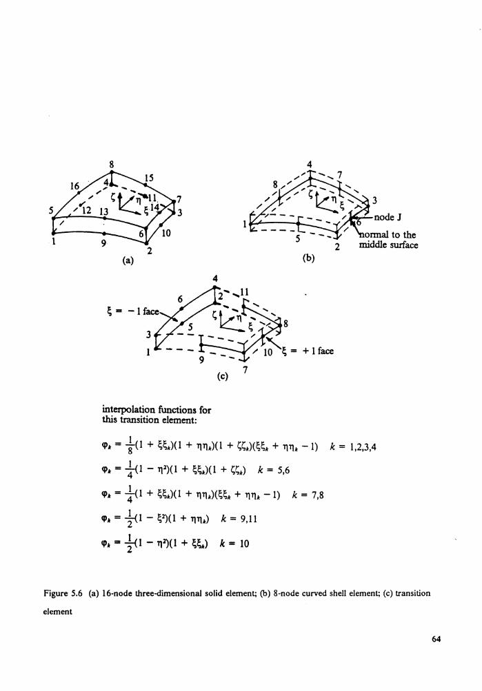
8 4
~ ~(:a 7
3 1~'}4.L-nodeJ
2 2 (a) (b)
3
1
interpolation functions for this transition element:
4
8
(c)
<i>.t = to + ;;.)(l + 1111•)(1 + l;l;.)(;;. + 1111• -1) k = 1,2,3,4
<i>.t = +< 1 - 'Ill)( 1 + ;;.)( 1 + t;t;.) k = 5,6
<!>.t = +<i + ;;.)(l + 1111.)(;;. + 1111• -1) k = 7,8
<!>.t = +1 - ; 2)(1 + 111i.) k = 9,11
cp. = +1 - 11l)(l + ;;.) k = 10
Figure 5.6 (a) 16-node three-dimensional solid element; (b) 8-node curved shell element; (c) transition
element
64
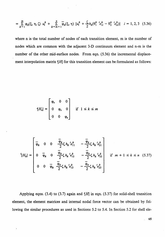
where n is the total number of nodes of each transition element, m is the number of
nodes which are common with the adjacent 3-D continuum element and n-m is the
number of the other mid-surface nodes. From eqn. (5.36) the incremental displace-
ment interpolation matrix 1H] for this transition element can be formulated as follows:
'[Hk] =
<9.t 0 0
1H.tl = 0 <9.t 0
0 0 <9.t
<9k 0 0 <9k h t k ~ k e11
0 <l>k 0 <9k h t k ~ k e12
0 0 <9k <l>k h t k ~ k e13
if I~k~m
~h tk - 2 k e11
<9k h t k - ~ k ei2 ifm+l~k~n (5.37)
<f>k t k - ~hk e13
Applying eqns. (3.4) to (3.7) again and 1H] in eqn. (5.37) for solid-shell transition
element, the element matrices and internal nodal force vector can be obtained by fol-
lowing the similar procedures as used in Sections 5.2 to 5.4. In Section 5.2 for shell ele-
65
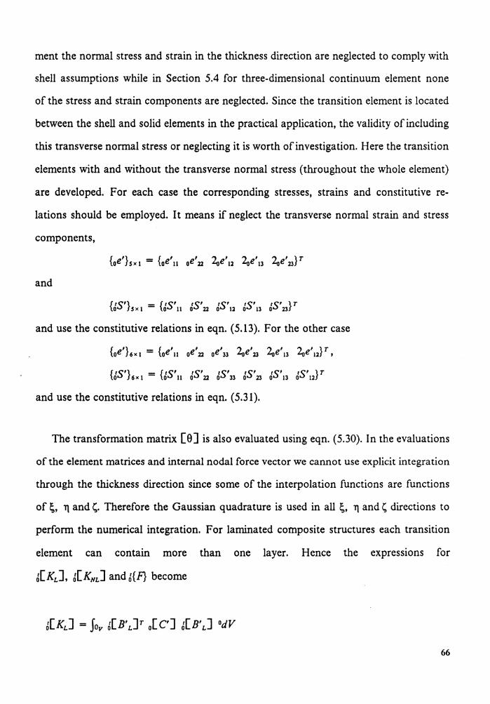
ment the normal stress and strain in the thickness direction are neglected to comply with
shell assumptions while in Section 5.4 for three-dimensional continuum element none
of the stress and strain components are neglected. Since the transition element is located
between the shell and solid elements in the practical application, the validity of including
this transverse normal stress or neglecting it is worth of investigation. Here the transition
elements with and without the transverse normal stress (throughout the whole element)
are developed. For each case the corresponding stresses, strains and constitutive re-
lations should be employed. It means if neglect the transverse normal strain and stress
components,
{ '} - { ' ' ") ' ") ' ") ' } T oe sx 1 - oe 11 oe 22 ~e 12 "1le 13 ~e 23
and
{ 1S'} - { 1S' 1S' 1S' 1S' 1S' } T 0 S x 1 - O 11 0 22 0 12 O 13 O 23
and use the constitutive relations in eqn. (5.13). For the other case
and use the constitutive relations in eqn. ( 5.31 ).
The transformation matrix [0] is also evaluated using eqn. (5.30). In the evaluations
of the element matrices and internal nodal force vector we cannot use explicit integration
through the thickness direction since some of the interpolation functions are functions
of~' 11 and'· Therefore the Gaussian quadrature is used in all ~' 11 and' directions to
perform the numerical integration. For laminated composite structures each transition
element can contain more than one layer. Hence the expressions for
66
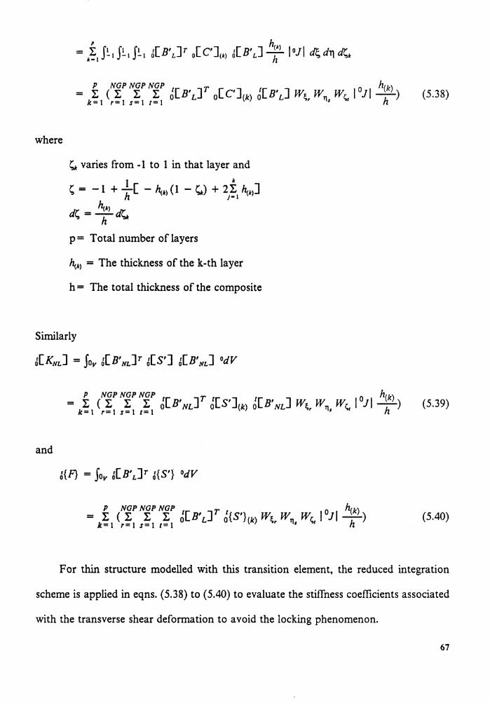
where
~ varies from -1 to I in that layer and I k
~ = - 1 + -h [ - ~k> ( 1 - ~) + 2 :t ~k1]
d~ =~Ir)~ h
p= Total number of layers
J•I
~"> = The thickness of the k-th layer
h = The total thickness of the composite
Similarly
J[KNLJ = Jov J[B'NL]r J[S'] J[B'NLJ 0dV
and
J{F} = Jov &[B' L]r J{S'} 0dV
(5.40)
For thin structure modelled with this transition element, the reduced integration
scheme is applied in eqns. (5.38) to (5.40) to evaluate the stiffness coefficients associated
with the transverse shear deformation to avoid the locking phenomenon.
67
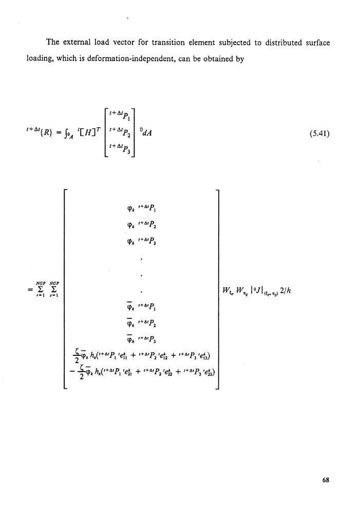
The external load vector for transition element subjected to distributed surface
loading, which is deformation-independent, can be obtained by
t+Mpl
t+M{R} = JoA '[H]T t+Mp2 odA
t+Atp3
NGP NGP = l: l:
r• l 1• l
<J>.1: 1+61 p 3
~;,; h ('+Mp 'ek + 1+Mp 'ek + 1+61p 'e*) 2 'f' k k 1 11 2 12 J 13
- f<PA: hk(1+61p1 'ei1 + t+MP2 'e~ + i+61pJ 'et)
(5.41)
68
where h is the thickness of the transition element at each Gaussian point and the order
of 1H 1{R} is [3m+5(n-m)] by 1.
69
CHAPTER 6
SAMPLE ANALYSIS
6. 1 Introduction
A number of representative problems were analyzed using the elements and solution
procedures developed in the present study. Some of the problems have the analytic
solutions or have been analyzed in the literature by using different finite-element models.
Comparisons of the present results with the solutions available in the literature can show
the accuracy and applicability of the formulations and elements in the present study. For
those problems which have not been analyzed yet the present results can be used as .
references for future investigations.
Static as well as transient analyses were performed for each kind of element developed
here. Newton-Raphson method was used for nonlinear transient analysis while modified
Riks/Wempner method was employed for post-buckling analysis. For most of the prob-
lems the reduced/selective integration scheme was used. Although many problems were
analyzed during this investigation, the results of only a few sample problems are pre-
sented in this Chapter.
6.2 Static Analysis
6.2.1 Plate and Shell Structures
1. A cylindrical shell roof under the action of self-weight
This problem, as shown in Fig. 6. l(a), has been used frequently for assesment of shell
finite element performance [55]. In Reference [55], the authors showed that with the all-
round reduction of integration order the parabolic and cubic shell elements show a more
70
rapid convergence and better accuracy than with the reduced integration order applied
to transverse shear terms only. The results obtained in the present study with 9-node
parabolic shell element and all-round reduction of integration order are shown in Fig.
6.1 (b) and 6.1 ( c ). The exact solution is solved by Scordelis [ 56]. Even with one element
the results have the tendency of exact solutions and for further subdivision the results
are close to the exact ones.
2. Simply-supported spherical shell subjected to a point load
The isotropic shell shown in Fig. 6.2(a) was analyzed for its large displacement re-
sponse with four 9-node elements and sixteen 4-node elements, modelling one-quarter
of the shell. Fig. 6.2(b) shows the responses calculated, including the post-buckling
range, with the modified Riks-Wempner method which automatically determines the
load increments. Fig. 6.2(b) also includes the results by Bathe [57].
3. Shallow cylindrical shell with a center point load
The isotropic shallow cylindrical shell under one concentrated load described in Fig.
6.3 is hinged at the longitudinal edges and free at the curved boundaries. The structure
exhibits snap-through as well as snap-back phenomena. One-quarter of the shell was
analyzed with four 9-node degenerated shell elements. The solution obtained by Crisfield
[45] is also shown in Fig. 6.3 to be compared with the present result.
4. 2-layer cross-ply(0/90) and angle-ply(-45/45) simply-supported plates
with uniform loading
The material properties of the lamina are:
£1/~ = 25, ~ = 7.031 x IOS N/cm2, G1J~ = 0.5, G13 = G12, G23/~ = 0.2, v12 = 0.25
The laminated plates in this problem do not buckle under the lateral uniform loading.
The modified Riks/Wempner method is adopted for nonlinear analyses of these two
plates. This method eliminates the difficulty to prescribe the load levels without an ap-
proximate knowledge of the load carrying capacity of the structure. Laminated
71
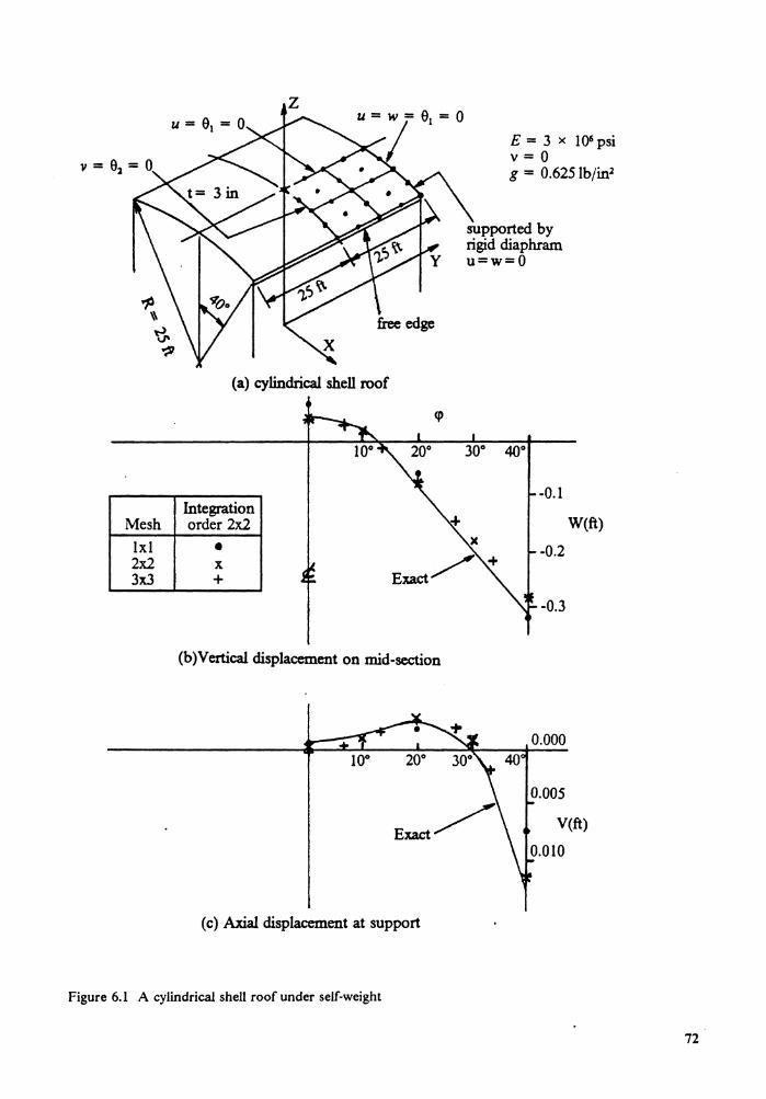
z
(a) cylindrical shell roof
Integration Mesh order 2x2 lxl • 2x2 x 3x3 +
(b)Vertical displacement on mid-section
10° 20°
(c) Axial displacement at support
Figure 6.1 A cylindrical shell roof under self-weight
E = 3 x 10⁶ psi v=O g = 0.625 lb/in2
supported by rigid diaphram u=w=O
30° 40°
-0.1
-0.2
-0.3
W(ft)
V(ft)
72
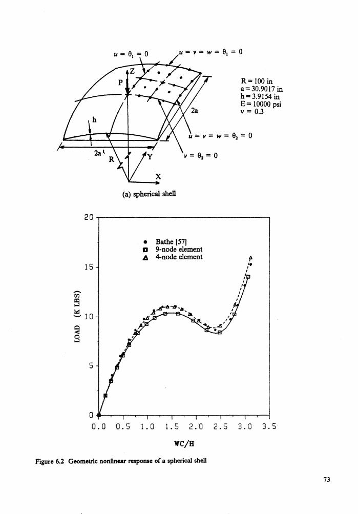
15
-C'/l
5
x (a) spherical shell
• Bathe (57] a 9-node element .6 4-node element
R= 100 in a= 30.9017 in h=3.9154in E= 10000 psi v = 0.3
~ 10
~ 5
o ..... -r--.----i.--~-r---r---ir--...---.--r--.~...---.----1 0.0 0.5 1.0 1.5 2.0 2.5 3.0 3.5
WC/B
Figure 6.2 Geometric nonlinear response of a spherical shell
73
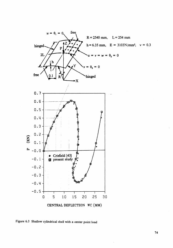
free R=2540 mm, L=254 mm
h=6.35 mm, E = 3103N/mm:i, v = 0.3
u=v=w=0::i=O
/ I
0.7 /
0.6
0.5
0.4
0.3
- 0.2 ~ o. 1 ........
~ -0.0
-o. 1 . • Crisfibld (45] . a piesent study •
-0.2
-0.3
-0.4
-0.5 o 5 10 15 20 25 30
CENTRAL DEFLECTION WC (MM)
Figure 6.3 Shallow cylindrical shell with a center point load
74
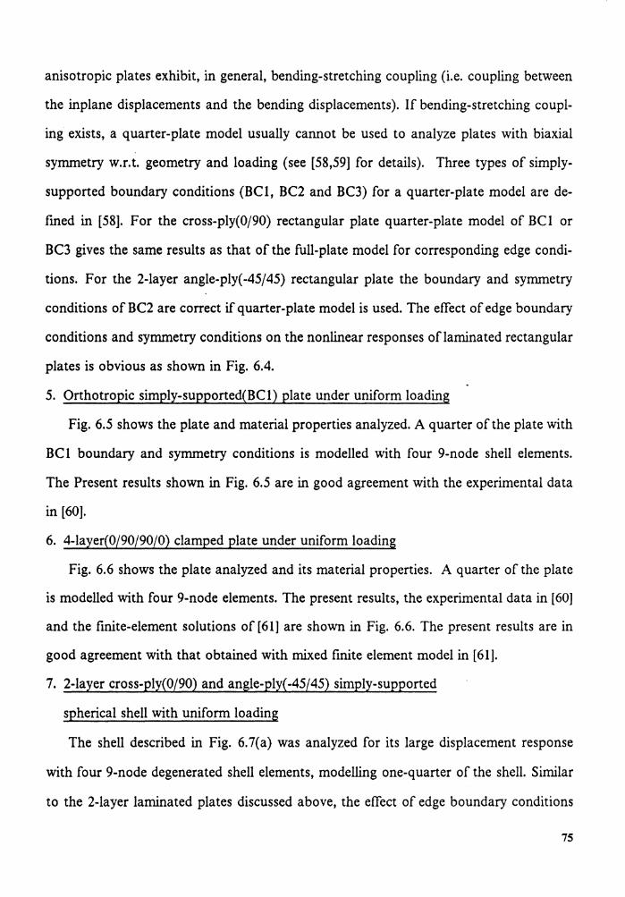
anisotropic plates exhibit, in general, bending-stretching coupling (i.e. coupling between
the inplane displacements and the bending displacements). If bending-stretching coupl-
ing exists, a quarter-plate model usually cannot be used to analyze plates with biaxial
symmetry w.r.t. geometry and loading (see [58,59] for details). Three types of simply-
supported boundary conditions (BCl, BC2 and BC3) for a quarter-plate model are de-
fined in [58]. For the cross-ply(0/90) rectangular plate quarter-plate model of BCl or
BC3 gives the same results as that of the full-plate model for corresponding edge condi-
tions. For the 2-layer angle-ply(-45/45) rectangular plate the boundary and symmetry
conditions of BC2 are correct if quarter-plate model is used. The effect of edge boundary
conditions and symmetry conditions on the nonlinear responses oflaminated rectangular
plates is obvious as shown in Fig. 6.4.
5. Orthotropic simply-supported(BCl) plate under uniform loading
Fig. 6.5 shows the plate and material properties analyzed. A quarter of the plate with
BC 1 boundary and symmetry conditions is modelled with four 9-node shell elements.
The Present results shown in Fig. 6.5 are in good agreement with the experimental data
in [60].
6. 4-layer(0/90/90/0) clamped plate under uniform loading
Fig. 6.6 shows the plate analyzed and its material properties. A quarter of the plate
is modelled with four 9-node elements. The present results, the experimental data in [60]
and the finite-element solutions of [61] are shown in Fig. 6.6. The present results are in
good agreement with that obtained with mixed finite element model in [61].
7. 2-layer cross-ply(0/90) and angle-ply(-45/45) simply-supported
spherical shell with uniform loading
The shell described in Fig. 6.7(a) was analyzed for its large displacement response
with four 9-node degenerated shell elements, modelling one-quarter of the shell. Similar
to the 2-layer laminated plates discussed above, the effect of edge boundary conditions
75
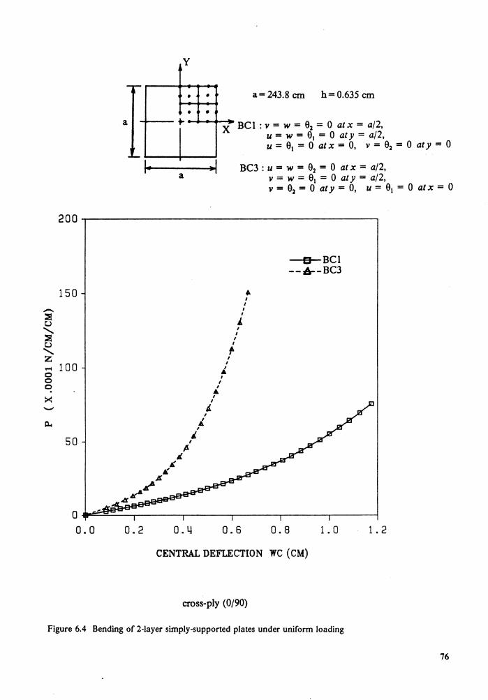
-::e t.>
......... ::e t.>
......... z .-4 0 0 0
>< '-'
c..
a
I·
150
100
50
I{ I{
~¥4 ~Jf.
y '
. ' • • I •
~ -
a ,.,
x
a= 243.8 cm h = 0.635 cm
BC 1 : v = w = 01 = 0 at x = a/2, u = w = 01 = 0 at y = a/2, u = 01 = 0 at x = 0, v = 01 = 0 aty = 0
BC3 : u = w = 02 = 0 at x = a/2,
• I I
I I
J. I
v = w = 01 = 0 at y = a/2, v = 01 = 0 aty = 0, u = 01 = 0 at x = 0
a BCl --4--BC3
I I
I ,. I
I I • I
I I • I
I
/. I
I. I
i I
~ 4
0 .... =:.!:"-=-~......-~~~...-~~~...-~~---.,...-~~-.,.~~~-1 0.0 0.2 0.4 0.6 0.8 1. 0 1. 2
CENTRAL DEFLECTION WC (CM)
cross-ply (0/90)
Figure 6.4 Bending of 2-layer simply-supported plates under uniform loading
76
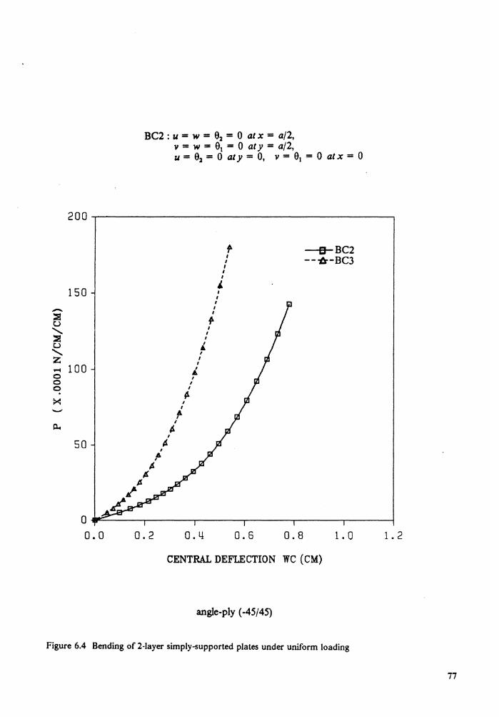
-;::!! u
.......... :::!!! u
......... z .-4 0 0 0
>< ..........
r:i..
200
150
100
50
BC2 : u = w = 02 = 0 at x = a/2, v = w = 01 = 0 at y = a/2, u = 02 = 0 at y = 0, v = 01 = 0 at x = 0
,. --&-BC2 I
--~-BC3 I I
I I
' I I
I I I ,.
I I
I
A. I
I I ..
I I
I
~ I ,
~ I
/& , p.
0 ..,,""-~~-"T-~~~-,-~~~--.-~~~--.-~~~-.~~~--i 0.0 0.2 0.4 0.6 0.8 1. 0 1. 2
CENTRAL DEFLECTION WC (CM)
angle-ply (-45/45)
Figure 6.4 Bending of 2-layer simply-supported plates under uniform loading
77
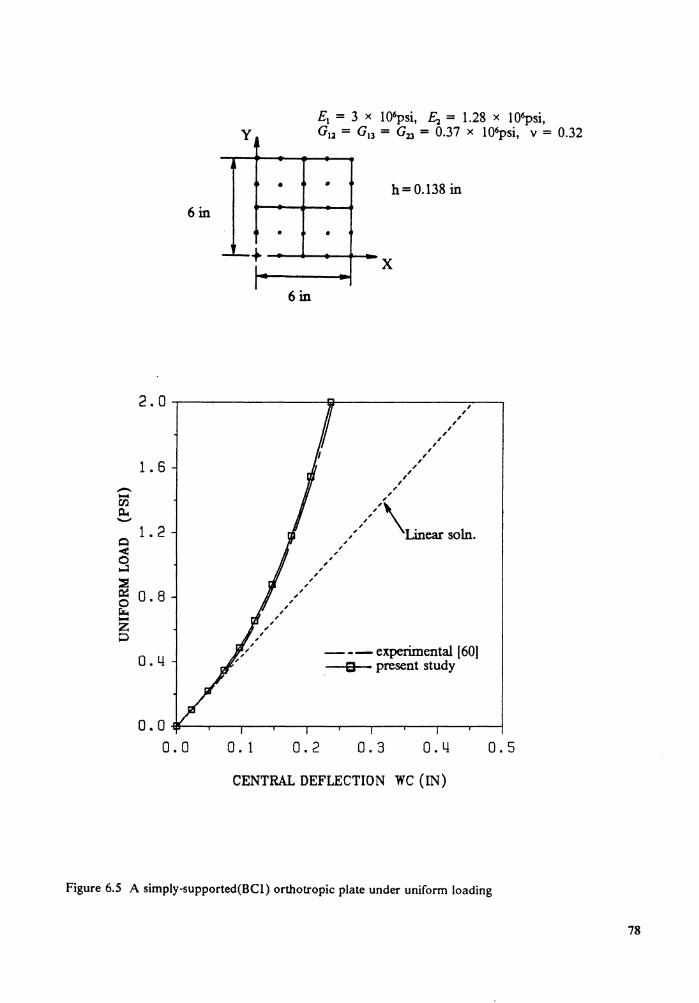
£1 = 3 x 10⁶psi, ~ = 1.28 x 10⁶psi, y G1l = G13 = Gll = 0.37 x 10⁶psi, v = 0.32
J
• • h= 0.138 in 6 in
' • • ----+
I x I
6 in
2.0 , , , , , , , , , , 1. 6
, ,, , , , - , , - , r:n
/,/\Linear soln. 0.. '-'
1. 2 0 , , < , 0 , ,, ...:I , ,,
~ , ,
0.8 , ,,
0 , r:r.. , , - , z , ,, ::> ,
0.4 ---experimental [60] a present study
0.0-llf---.----r--.------r----.--.---.--.---.----j 0.0 0. 1 0.2 0.3 0.4 0.5
CENTRAL DEFLECTION WC (IN)
Figure 6.5 A simply-supported(BCI) orthotropic plate under uniform loading
78
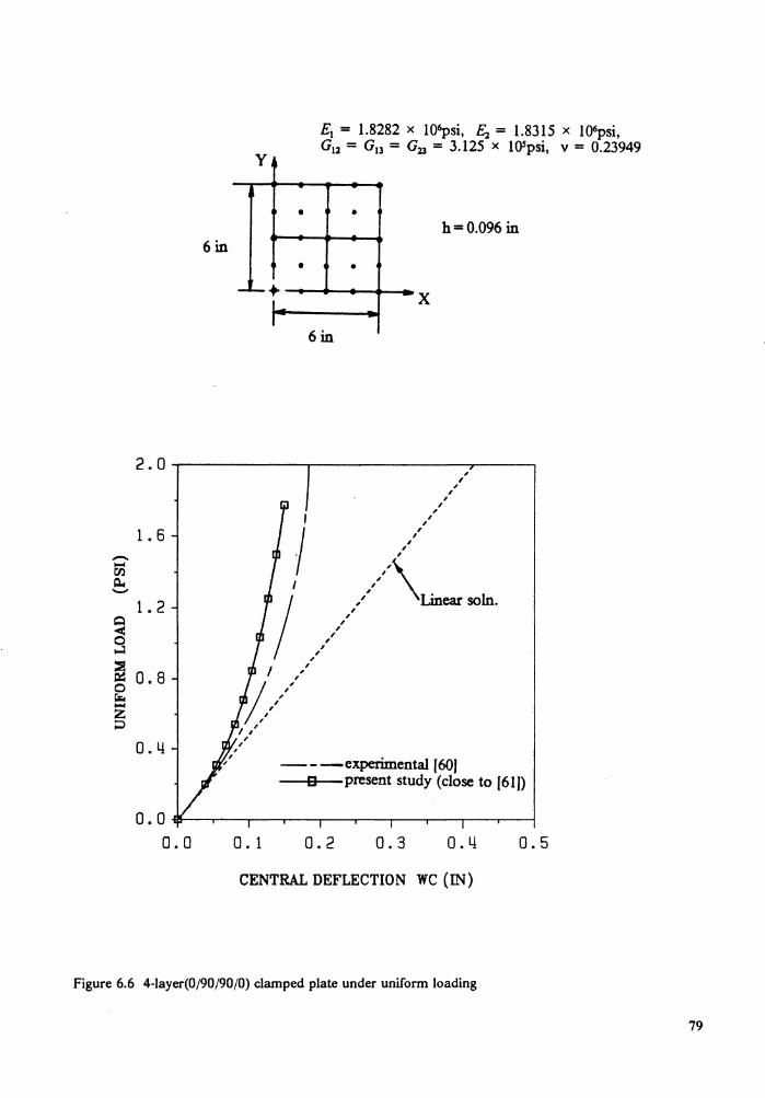
Ya -•
6 in •
--+ -I -I
E1 = 1.8282 x 10⁶psi, £i = 1.8315 x 10⁶psi, G12 = G13 = G23 = 3.125 x lOSpsi, v = 0.23949
-•
h=0.096 in -
• - x
6m
Figure 6.6 4-layer(0/90/90/0) clamped plate under uniform loading
79
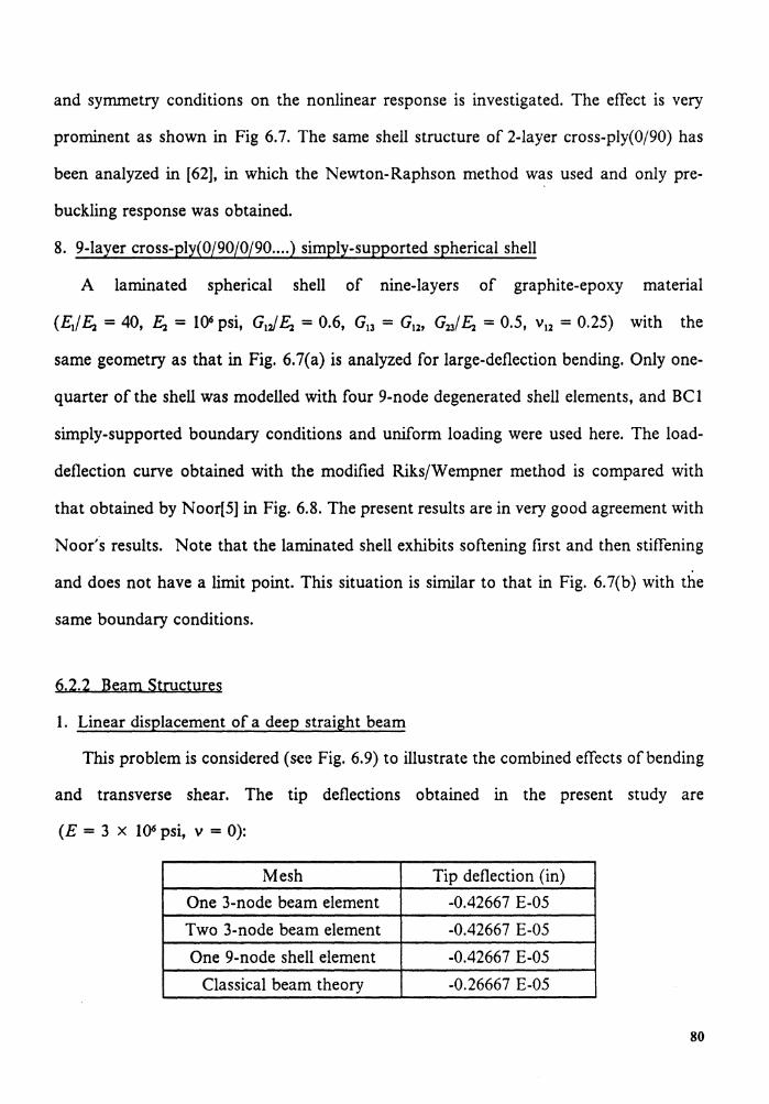
and symmetry conditions on the nonlinear response is investigated. The effect is very
prominent as shown in Fig 6. 7. The same shell structure of 2-layer cross-ply(0/90) has
been analyzed in [62], in which the Newton-Raphson method was used and only pre-
buckling response was obtained.
8. 9-layer cross-ply(0/90/0/90 .... ) simply-supported spherical shell
A laminated spherical shell of nine-layers of graphite-epoxy material
same geometry as that in Fig. 6.7(a) is analyzed for large-deflection bending. Only one-
quarter of the shell was modelled with four 9-node degenerated shell elements, and BCl
simply-supported boundary conditions and uniform loading were used here. The load-
deflection curve obtained with the modified Riks/Wempner method is compared with
that obtained by Noor[5] in Fig. 6.8. The present results are in very good agreement with
Noor's results. Note that the laminated shell exhibits softening first and then stiffening
and does not have a limit point. This situation is similar to that in Fig. 6. 7(b) with the
same boundary conditions.
6.2.2 Beam Structures
1. Linear displacement of a deep straight beam
This problem is considered (see Fig. 6.9) to illustrate the combined effects of bending
and transverse shear. The tip deflections obtained in the present study are
(E = 3 x 10⁶ psi, v = 0):
Mesh Tip deflection (in) One 3-node beam element -0.42667 E-05 Two 3-node beam element -0.42667 E-05 One 9-node shell element -0.42667 E-05
Classical beam theory -0.26667 E-05
80
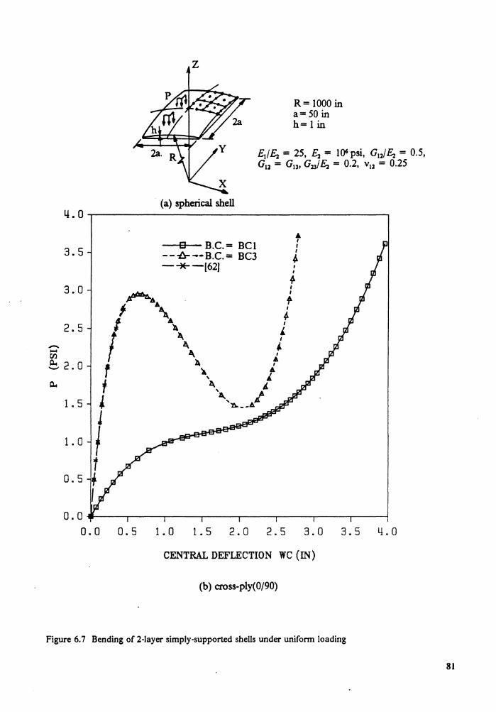
z
(a) spherical shell Y.O
8 B.C.= BCl 3.5 - - -l:r -- B.C. = BC3 -*"-(62)
3.0 ~AA I ~~ 2.5 --00
R= 1000 in a= 50 in h= 1 in
A I I I • I
' .f. I I
f-I
" I
J.. I
" I I \ ~ 2. 0 .A r ~\, I
A I
A Q.. t ~ ' 1. 5 l '~, ta
-r.. _ -"' J
1. 0 t 1
0.5 I
0.0--~--.~~--r-~~-.--~--..-~~--.-~~..--~-,..~--1
0.0 0.5 1.0 1.5 2.0 2.5 3.0 3.5 4.0
CENTRAL DEFLECTION WC (IN)
(b) cross-ply(0/90)
Figure 6. 7 Bending of 2-layer simply-supported shells under uniform loading
81
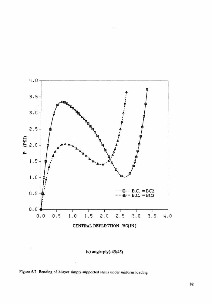
3.5
3.0
2.5 --Cl)
~ 2. 0
1. 5
1. 0
0.5
~ I I I
J. I I I
A I I I
.6. I I
~ , t-• i
j.
t ,
8 B.C. =BC2 - --tr- B.C. = BC3
0.0---~~...--~---.~~---.-~~--,-~~--.--~~-.--~~.--~---1
0.0 0.5 1. 0 1. 5 2.0 2.5 3. 0 3.5 4.0
CENTRAL DEFLECTION WC(IN)
( c) angle-ply( -45/45)
Figure 6. 7 Bending of 2-layer simply-supported shells under uniform loading
82
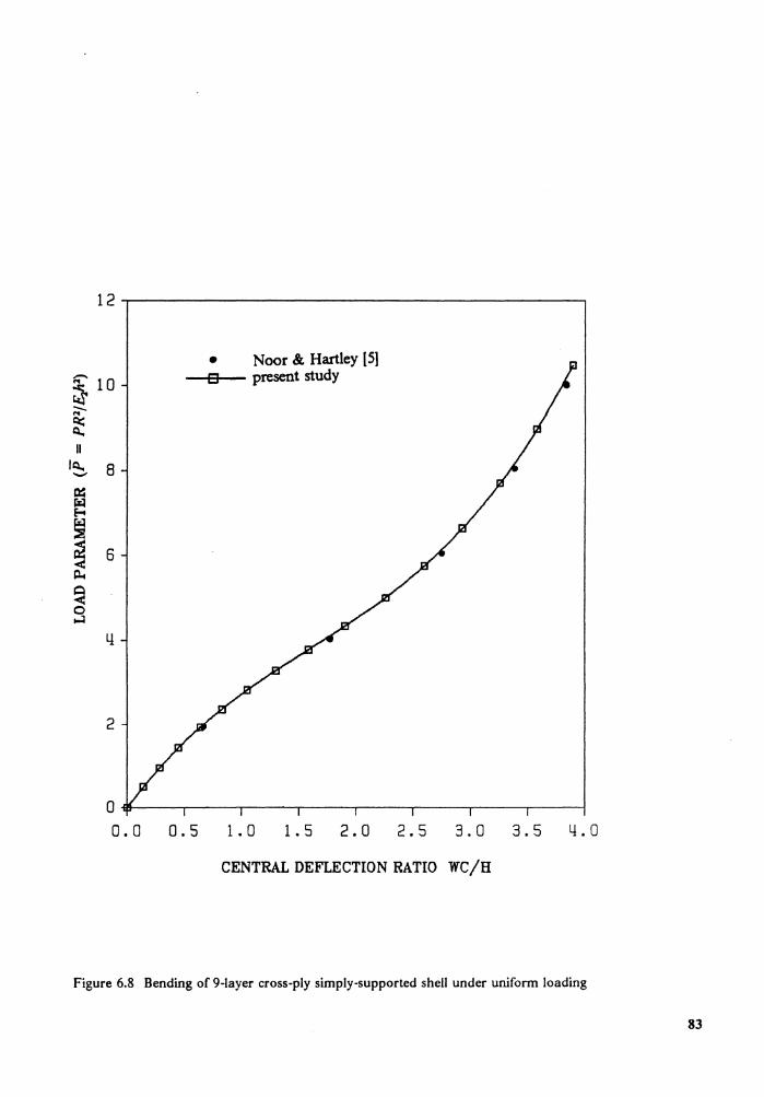
• Noor & Hartley [ 5) - 8 present study .... 10 ~ -.... ~ II
IQ.. 8 -~ ~ E-.
~ ~ 6 i:i..
~ 0 ...:l
l!
2
0 1ft-~~~~~~~~--.-~~--.-~~--.-~~-.-~~-.-~~-l 0.0 0.5 1. 0 1. 5 2.0 2.5 3.0 3.5 4.0
CENTRAL DEFLECTION RATIO WC/H
Figure 6.8 Bending of 9-layer cross-ply simply-supported shell under uniform loading
83
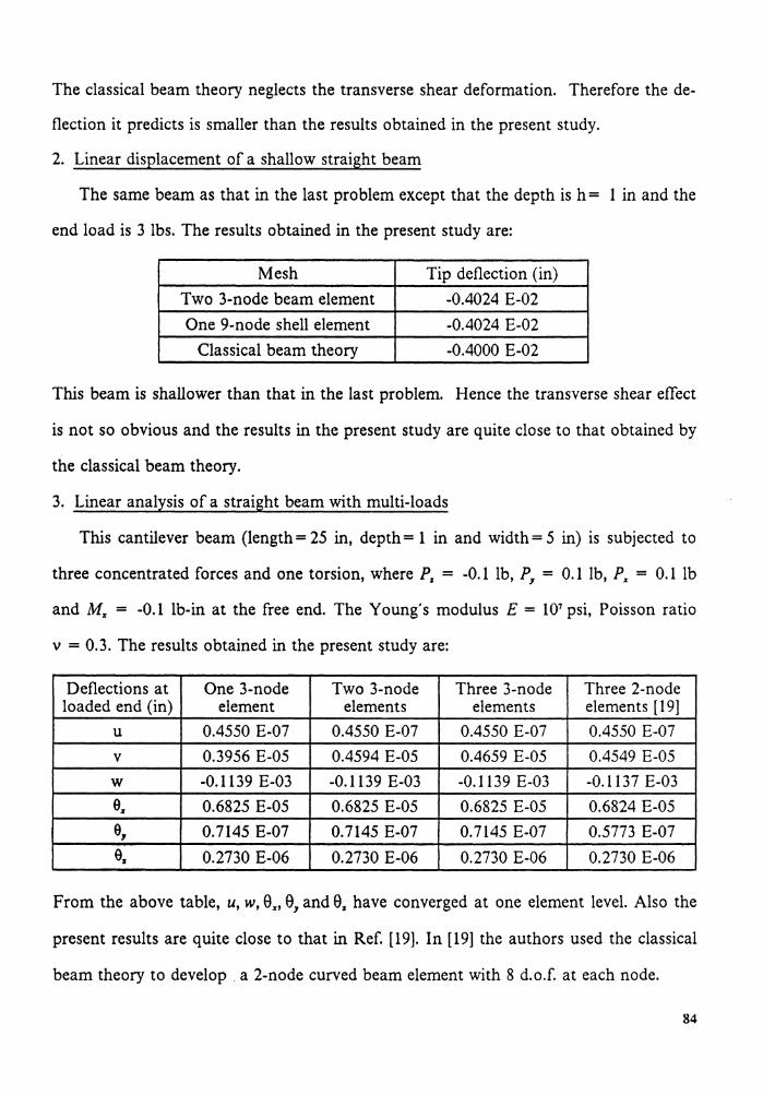
The classical beam theory neglects the transverse shear deformation. Therefore the de-
flection it predicts is smaller than the results obtained in the present study.
2. Linear displacement of a shallow straight beam
The same beam as that in the last problem except that the depth is h = 1 in and the
end load is 3 lbs. The results obtained in the present study are:
Mesh Tip deflection (in) Two 3-node beam element -0.4024 E-02 One 9-node shell element -0.4024 E-02
Classical beam theory -0.4000 E-02
This beam is shallower than that in the last problem. Hence the transverse shear effect
is not so obvious and the results in the present study are quite close to that obtained by
the classical beam theory.
3. Linear analysis of a straight beam with multi-loads
This cantilever beam (length= 25 in, depth= 1 in and width= 5 in) is subjected to
three concentrated forces and one torsion, where P2 = -0.1 lb, P, = 0.1 lb, P, = 0.1 lb
and M. = -0.1 lb-in at the free end. The Young's modulus E = 107 psi, Poisson ratio
v = 0.3. The results obtained in the present study are:
Deflections at One 3-node Two 3-node Three 3-node Three 2-node loaded end (in) element elements elements elements [ 19]
u 0.4550 E-07 0.4550 E-07 0.4550 E-07 0.4550 E-07 v 0.3956 E-05 0.4594 E-05 0.4659 E-05 0.4549 E-05 w -0.1139 E-03 -0.1139 E-03 -0.1139 E-03 -0.1137 E-03 e .. 0.6825 E-05 0.6825 E-05 0.6825 E-05 0.6824 E-05 e, 0.7145 E-07 0.7145 E-07 0.7145 E-07 0.5773 E-07 e. 0.2730 E-06 0.2730 E-06 0.2730 E-06 0.2730 E-06
From the above table, u, w, 0,, 0, and 02 have converged at one element level. Also the
present results are quite close to that in Ref. [ 19]. In [ 19] the authors used the classical
beam theory to develop . a 2-node curved beam element with 8 d.o.f. at each node.
84
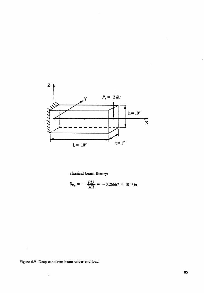
z
I I
h= 10·
.)---------- -
~ .P=1· L= 10'
classical beam theory:
On,, = - Pl3 = - 0.26667 x 10-s in 3EI
Figure 6.9 Deep cantilever beam under end load
x
SS
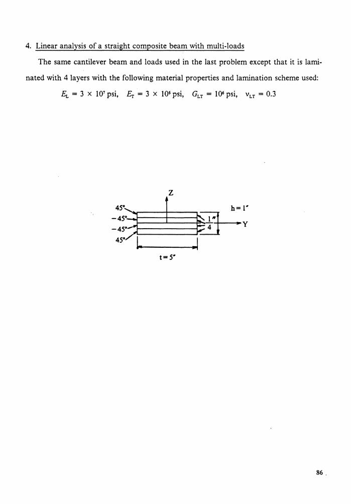
4. Linear analysis of a straight composite beam with multi-loads
The same cantilever beam and loads used in the last problem except that it is lami-
nated with 4 layers with the following material properties and lamination scheme used:
Er, = 3 x 10⁷ psi, Er = 3 x 10⁶ psi, GLT = 106 psi, vLT = 0.3
z
t= 5"
86.
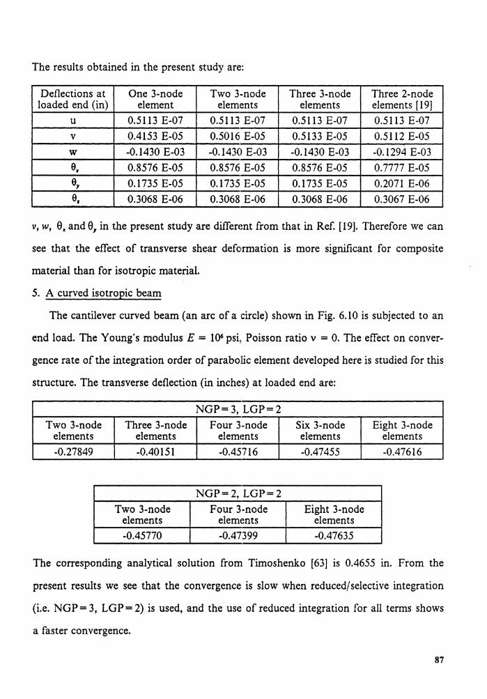
The results obtained in the present study are:
Deflections at One 3-node Two 3-node Three 3-node Three 2-node loaded end (in) element elements elements elements [ 19]
u 0.5113 E-07 0.5113 E-07 0.5113 E-07 0.5113 E-07 v 0.4153 E-05 0.5016 E-05 0.5133 E-05 0.5112 E-05 w -0.1430 E-03 -0.1430 E-03 -0.1430 E-03 -0.1294 E-03 a .. 0.8576 E-05 0.8576 E-05 0.8576 E-05 0.7777 E-05 a, 0.1735 E-05 0.1735 E-05 0.1735 E-05 0.2071 E-06 a. 0.3068 E-06 0.3068 E-06 0.3068 E-06 0.3067 E-06
v, w, 0 .. and 0, in the present study are different from that in Ref. [19]. Therefore we can
see that the effect of transverse shear deformation is more significant for composite
material than for isotropic material.
5. A curved isotropic beam
The cantilever curved beam (an arc of a circle) shown in Fig. 6.10 is subjected to an
end load. The Young's modulus E = 106 psi,. Poisson ratio v = 0. The effect on conver-
gence rate of the integration order of parabolic element developed here is studied for this
structure. The transverse deflection (in inches) at loaded end are:
NGP= 3, LGP= 2 Two 3-node Three 3-node Four 3-node Six 3-node Eight 3-node
elements elements elements elements elements -0.27849 -0.40151 -0.45716 -0.47455 -0.47616
NGP=2, LGP=2 Two 3-node Four 3-node Eight 3-node
elements elements elements -0.45770 -0.47399 -0.47635
The corresponding analytical solution from Timoshenk.o [63] is 0.4655 in. From the
present results we see that the convergence is slow when reduced/selective integration
(i.e. NGP= 3, LGP= 2) is used, and the use of reduced integration for all terms shows
a faster convergence.
87
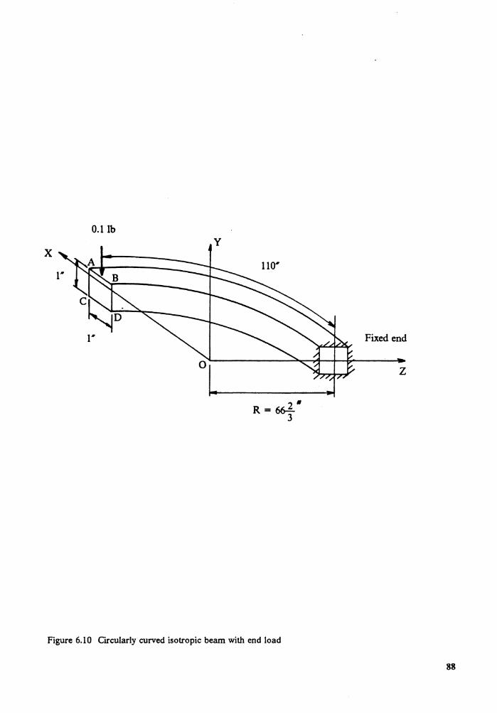
0.1 lb
x y
R=~· 3
Figure 6.10 Circularly curved isotropic beam with end load
Fixed end
z
88
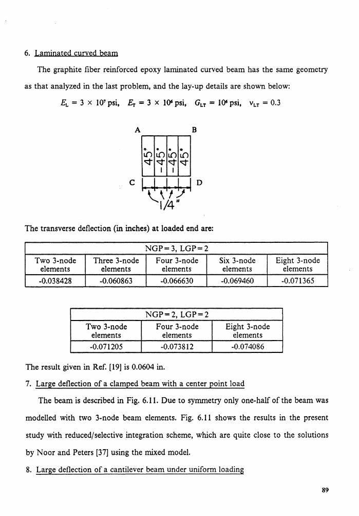
6. Laminated curved beam
The graphite fiber reinforced epoxy laminated curved beam has the same geometry
as that analyzed in the last problem, and the lay-up details are shown below:
EL = 3 x 10' psi, Er = 3 x 10' psi, GLT = 10' psi, vLT = 0.3
A B
0 • • 0 \{') LO L{) LO cq- .q- cq- cq-
I I
C 1 •• 1. .1 •• 1. ~ D ~. \ '/ "1/4 ti
The transverse deflection (in inches) at loaded end are:
NGP= 3, LGP= 2 Two 3-node Three 3-node Four 3-node
elements elements elements -0.038428 -0.060863 -0.066630
NGP=2, LGP=2 Two 3-node Four 3-node
elements elements -0.071205 -0.073812
The result given in Ref. [ 19] is 0.0604 in.
Six 3-node elements -0.069460
Eight 3-node elements -0.074086
7. Large deflection of a clamped beam with a center point load
Eight 3-node elements -0.071365
The beam is described in Fig. 6.11. Due to symmetry only one-half of the beam was
modelled with two 3-node beam elements. Fig. 6.11 shows the results in the present
study with reduced/selective integration scheme, which are quite close to the solutions
by Noor and Peters [37] using the mixed model.
8. Large deflection of a cantilever beam under uniform loading
89
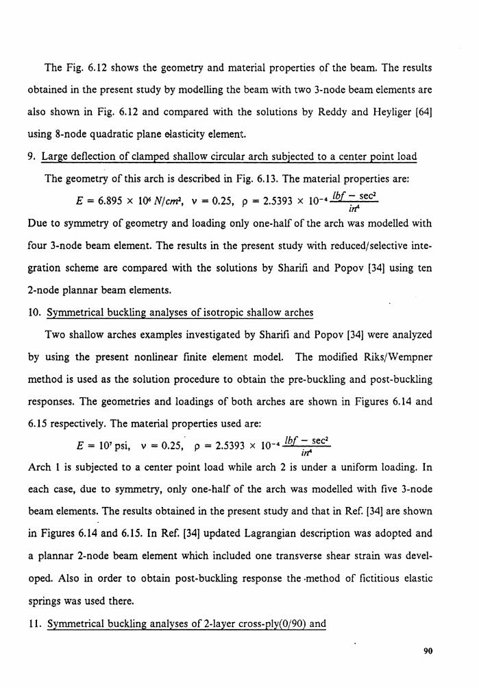
The Fig. 6.12 shows the geometry and material properties pf the beam. The results
obtained in the present study by modelling the beam with two 3-node beam elements are
also shown in Fig. 6.12 and compared with the solutions by Reddy and Heyliger [64]
using 8-node quadratic plane elasticity element.
9. Large deflection of clamped shallow circular arch subjected to a center point load
The geometry of this arch is described in Fig. 6.13. The material properties are:
E = 6.895 x 10⁶ N/cm2, v = 0.25, p = 2.5393 x 10⁻⁴ lb[ ~sec2
Due to symmetry of geometry and loading only one-half of the arch was modelled with
four 3-node beam element. The results in the present study with reduced/selective inte-
gration scheme are compared with the solutions by Sharifi and Popov [34] using ten
2-node plannar beam elements.
10. Symmetrical buckling analyses of isotropic shallow arches
Two shallow arches examples investigated by Sharifi and Popov [34] were analyzed
by using the present nonlinear finite element model. The modified Riks/\Vempner
method is used as the solution procedure to obtain the pre-buckling and post-buckling
responses. The geometries and loadings of both arches are shown in Figures 6.14 and
6.15 respectively. The material properties used are:
E = 101 psi, v = 0.25,. p = 2.5393 x 10⁻⁴ lb( ~ sec2
Arch 1 is subjected to a center point load while arch 2 is under a uniform loading. In
each case, due to symmetry, only one-half of the arch was modelled with five 3-node
beam elements. The results obtained in the present study and that in Ref. [34] are shown
in Figures 6.14 and 6.15. In Ref. [34] updated Lagrangian description was adopted and
a plannar 2-node beam element which included one transverse shear strain was <level-
oped. Also in order to obtain post-buckling response the ·method of fictitious elastic
springs was used there.
11. Symmetrical buckling analyses of 2-layer cross-ply(0/90) and
90
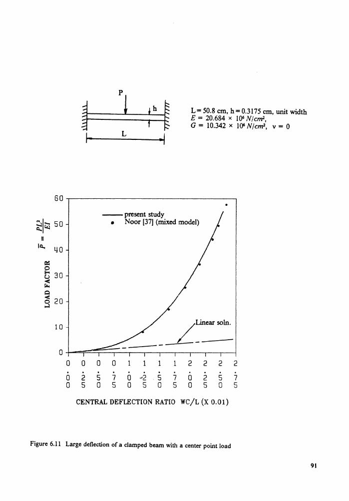
60
~1~ 50 II
IQ.. YO a:: 0 t> 30 < ~ Q < 20 0 ...:l
10
0 0 . a a
J-
•
a a a . . . 2 5 7 5 a 5
L ·I
present study
L= 50.8 cm, h= 0.3175 cm, unit width E = 20.684 x 10⁶ N/cm2, G = 10.342 x 10⁶ N/cm2, v = 0
•
Noor [37] (mixed model)
/_~soln.
1 1 1 1 2 2 2 2 . . . . . . . . 0 ... 2 .5 7 a 2 5 7 a 5 a 5 0 5 0 5
CENTRAL DEFLECTION RATIO WC/L (X 0.01)
Figure 6.11 Large deflection of a clamped beam with a center point load
91
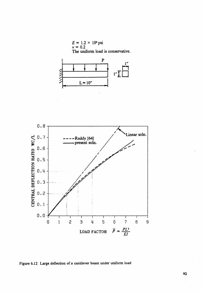
0.8
~ o. 7 u f!I: 0 0.6
~ 0.5 z 0 .....
0.4-~ -··· .. u r.;;i
&: 0.3 r.;;i Q
~ 0.2 ~ z r.;;i 0. 1 u
0.0 0 1
E = 1.2 x 10⁴ psi v = 0.2 The uniform load is conservative.
p
/
----Reddy (64] / Linear soln.
-present soln.
2 3 5
LOAD FACTOR
6 7 - PL3 P=-
EI
8
Figure 6.12 Large deflection of a cantilever beam under uniform load
9
92
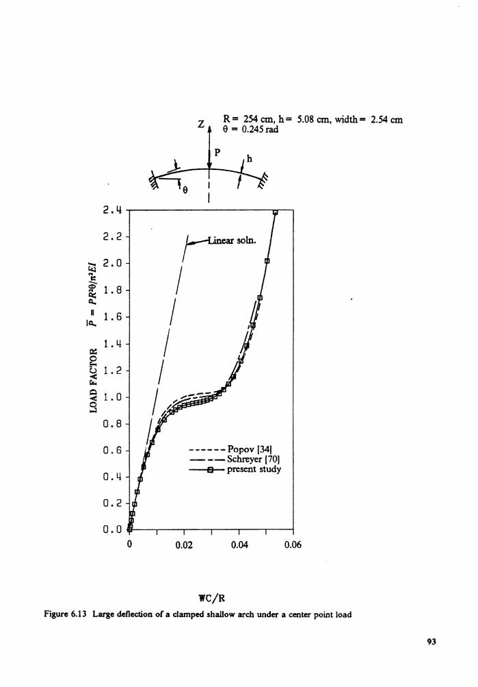
2.4
2.2
~ 2.0 .. II:: -Ct> 1. 8 ... ~ Q.,
II 1. 6 IQ.,
1. 4 I 0:: 0
I e.. 1. 2 ~ tJ;.. Q 1. 0 < 0 ...:I
0.8
0.6
0.4
0.2
0.0 0
I I
z
p
R = 254 cm, h = 5.08 cm, width= 2.54 cm 0 = 0.245rad
/earsoln.
------Popov [34) - --Schreyer (70)
B present study
0.02 0.04 0.06
WC/R Figure 6.13 Large deflection of a clamped shallow arch under a center point load
93
angle-ply(-45/45) shallow arches
The geometries and loading of these two 2-layer composite arches are the same as
that of arch 1 in the last problem. The material properties are:
£ 1/ E,. = 25, E,. = 106 psi, G1J E,. = 0.5, G13 = G12,
GD/ E,. = 0.2, V12 = 0.25, p = 2.3763 x 10-s lb{~ sec2
Since the symmetrical deformation modes exist for both arches, only one-half of the arch
was modelled by five 3-node beam elements for each beam. The pre- and post-buckling
responses obtained in the present study with the modified Riks/Wempner method are
shown in Fig. 6.16.
6.2.3 Stiffened Plates and Shells
1. Analysis of a stiffened plate with eccentric stiffeners
This problem shown in Fig. 6.17 illustrates the use of the degenerated shell element
in conjunction with the degenerated beam element developed in the present study. The
nodes are located on the midplane of the plate and the stiffness of stiffeners are added
to that of the shell elements without any additional degrees-of-freedom. The
reduced/selective integration scheme was used to evaluate the stiffness matrices of shell
and beam elements. The present results are compared with the solution calculated using
the classical beam theory. They are shown below ( where NGP = the number of inte-
gration point with the bending part, LGP = the number of integration point with the
transverse shear part):
Transverse Mesh NGP LGP deflection (in)
One 9-node shell element and Two 3-node beam elements 3 2 -0.25447 E-03
Two 9-node shell elements and Four 3-node beam elements 3 2 -0.25533 E-03
Classical beam theory -0.25195 E-03
94
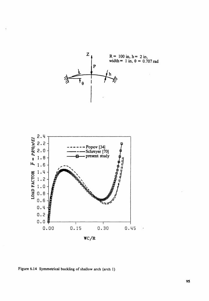
z
p
R = 100 in, h = 2 in, width= I in, 9 = 0. 707 rad
..... 2. 4 .....------------------, ~ 1::2.2 -a:> Q::2.0 ~ II 1. 8
IQ.. 1 . 6
1. 0 0.8 0.6 0.4 0.2
------Popov [34) ---Schreyer [70) --a..._-present study
0.0-m------.------,...--------i 0.00 0. 15 0.30 0.45
WC/R
Figure 6.14 Symmetrical buck.ling of shallow arch (arch 1)
9S
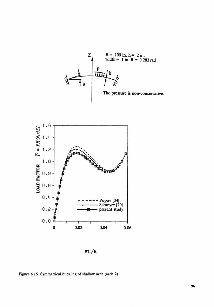
~ 1. 6
... a:: a;- 1. L! ... ~ ~
II 1. 2 I~
1. 0 c:: 0 e-... 0.8 C..> ~ Q 0.6 < 0 ~
0. L!
0.2
0.0 0
Z R = 100 in, h = 2 in, width= I in, 0 = 0.283 rad
The pressure is non-conservative.
- - ---- Popov (34) - - - Schreyer [70)
D present study
0.02 0.04 0.06
WC/R
Figure 6.15 Symmetrical buckling of shallow arch (arch 2)
96
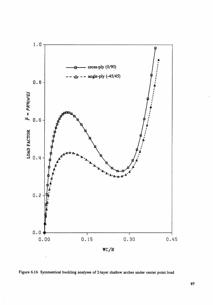
o cross-ply (0/90)
- - -tr - - angle-ply (-45/45) 0.8
~ .... ~
CI>"
~ II
IQ.. 0. 6
0.2
o.o--~~~~~~~..-~~~~~~----.~~~~~~~-t
0.00 0. 15 0.30 0.45
WC/R
Figure 6.16 Symmetrical buckling analyses of 2-layer shallow arches under center point load
97
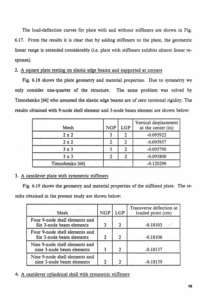
The load-deflection curves for plate with and without stiffeners are shown in Fig.
6.17. From the results it is clear that by adding stiffeners to the plate, the geometric
linear range is extended considerably (i.e. plate with stiffeners exhibits almost linear re-
sponse).
2. A square plate resting on elastic edge beams and supported at corners
Fig. 6.18 shows the plate geometry and material properties. Due to symmetry we
only consider one-quarter of the structure. The same problem was solved by
Timoshenko [66] who assumed the elastic edge beams are of zero torsional rigidity. The
results obtained with 9-node shell element and 3-node beam element are shown below:
Vertical displacement Mesh NGP LGP at the center (in) 2x2 3 2 -0.095922 2x2 2 2 -0.095957 3x3 3 2 -0.095790 3x3 2 2 -0.095800
Timoshenko [66) -0.120290
3. A cantilever plate with symmetric stiffeners
Fig. 6.19 shows the geometry and material properties of the stiffened plate. The re-
suits obtained in the present study are shown below:
Transverse deflection at Mesh NGP LGP loaded point (cm)
Four 9-node shell elements and Six 3-node beam elements 3 2 -0.18103 /
//
Four 9-node shell elements and Six 3-node beam elements 2 2 -0.18106
Nine 9-node shell elements and nine 3-node beam elements 3 2 -0.18137
Nine 9-node shell elements and nine 3-node beam elements 2 2 -0.18139
4. A cantilever cylindrical shell with symmetric stiffeners
98
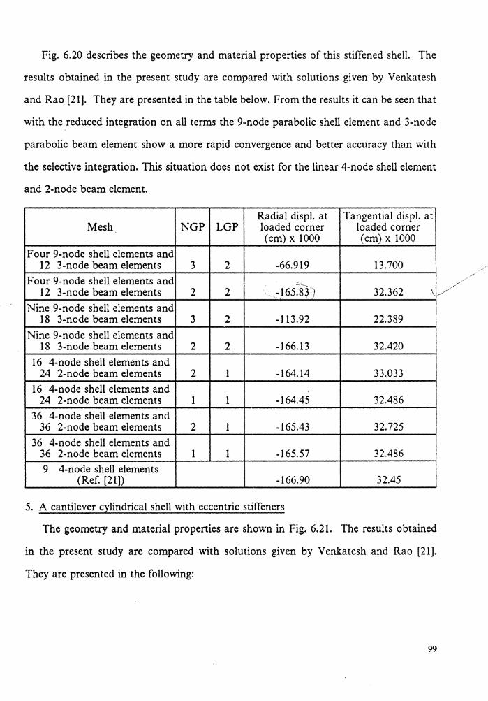
Fig. 6.20 describes the geometry and material properties of this stiffened shell. The
results obtained in the present study are compared with solutions given by Venkatesh
and Rao [21]. They are presented in the table below. From the results it can be seen that
with the reduced integration on all terms the 9-node parabolic shell element and 3-node
parabolic beam element show a more rapid convergence and better accuracy than with
the selective integration. This situation does not exist for the linear 4-node shell element
and 2-node beam element.
Radial displ. at Tangential displ. at Mesh NGP LGP loaded comer loaded corner
(cm) x 1000 (cm) x 1000 Four 9-node shell elements and
12 3-node beam elements 3 2 -66.919 13.700 Four 9-node shell elements and
12 3-node beam elements 2 2 , -165.Sf) 32.362 \
Nine 9-node shell elements and 18 3-node beam elements 3 2 -113.92 22.389
Nine 9-node shell elements and 18 3-node beam elements 2 2 -166.13 32.420
16 4-node shell elements and 24 2-node beam elements 2 1 -164.14 33.033
16 4-node shell elements and 24 2-node beam elements 1 l -164.45 32.486
36 4-node shell elements and 36 2-node beam elements 2 1 -165.43 32.725
36 4-node shell elements and 36 2-node beam elements 1 l -165.57 32.486 9 4-node shell elements
(Ref. [21]) -166.90 32.45
5. A cantilever cylindrical shell with eccentric stiffeners
The geometry and material properties are shown in Fig. 6.21. The results obtained
in the present study are compared with solutions given by Venkatesh and Rao [21 ].
They are presented in the following:
99
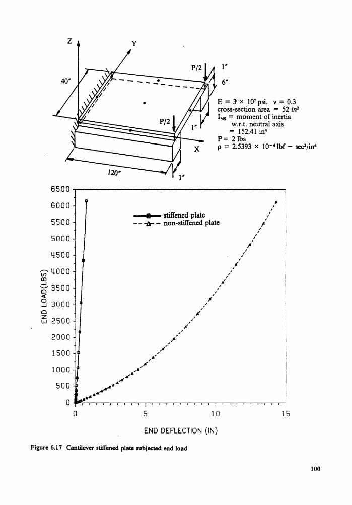
z
6500
6000
5500
5000
4500
(/)' 4000 m .g- 3500 <{ 0 3000 _J
0 z 2500 w
2000
1500
1000
500
0 0
y
B stiffened plate
1'"'
6*
E = 3· x 107 psi, v = 0.3 cross-section area = 52 in2 INS = moment of inertia
w.r.t. neutral axis = 152.41 in4
P= 2 lbs p = 2.5393 x 10-• lbf - sec2/in4
' I
, , ,..
- - -tJr - non-stiffened plate ,
!
J(
5
, , , /I
, , , ,
10
END DEFLECTION (IN)
• I , , , I ,
,• , , ,
I I
, , ,
15
Figure 6.17 Cantilever stiffened plate subjected end load
100
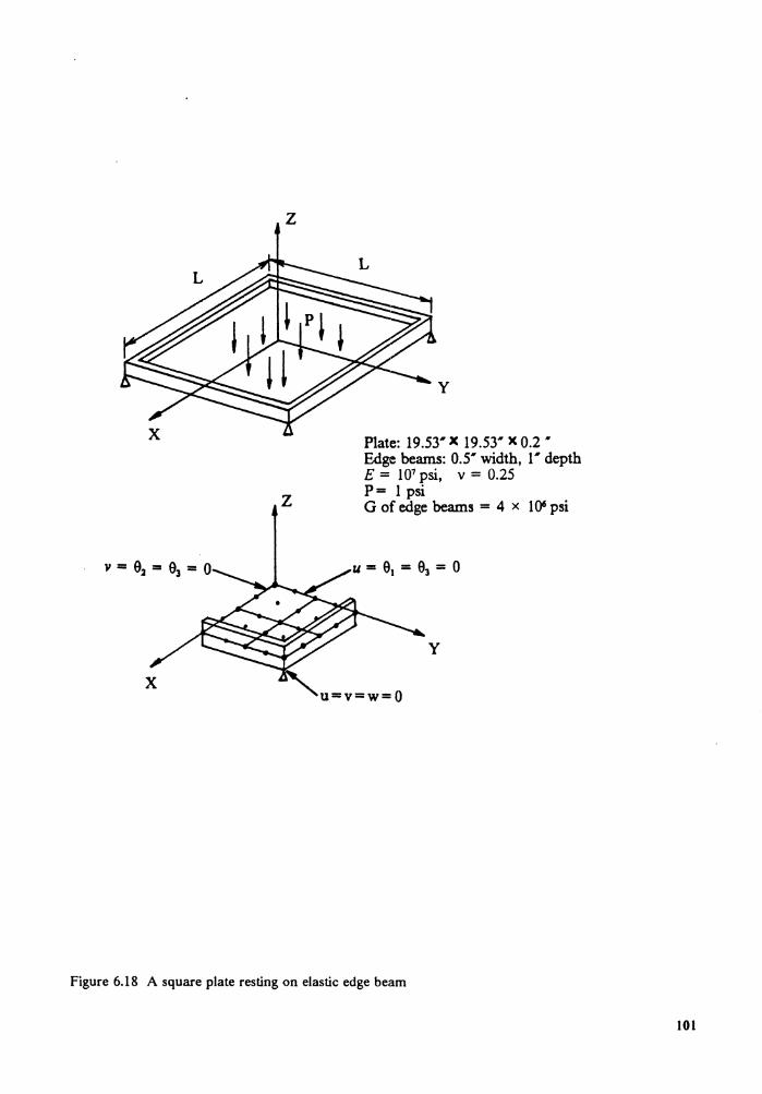
z
z
y
Plate: 19.53' x 19.53' x 0.2 • Edge beams: 0.5' width, i • depth E = 107 psi, v = 0.25 P= 1 psi G of edge beams = 4 x 10⁶ psi
Figure 6.18 A square plate resting on elastic edge beam
101
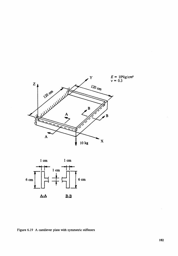
z
10 kg
lcm lcm
Figure 6.19 A cantilever plate with symmetric stiffeners
x
E = l()6kg/cm2 v = 0.3
102
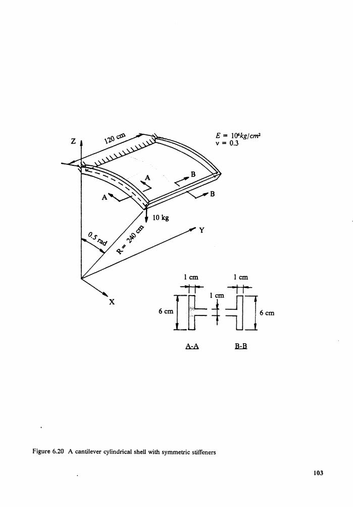
z
x
y
E = 106kg/cm1 v = 0.3
lcm lcm
Figure 6.20 A cantilever cylindrical shell with symmetric stiffeners
103
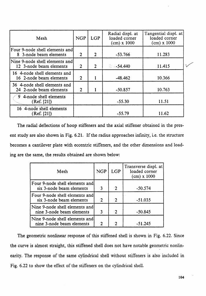
Radial displ. at Tangential displ. at Mesh NGP LGP loaded corner loaded corner
(cm) x 1000 (cm) x 1000 Four 9-node shell elements and
8 3-node beam elements 2 2 -53.766 11.283 Nine 9-node shell elements and
12 3-node beam elements 2 2 '-54.440 11.415 16 4-node shell elements and
16 2-node beam elements 2 1 -48.462 10.366 36 4-node shell elements and
24 2-node beam elements 2 1 -50.857 10.763 ./g' 4-node shell elements \ (Ref. [21]) -55.30 11.51 ,,_ -...
--~- - ---~-----------·-··.
16 4-node shell elements (Ref. [21]) -55.79 11.62
The radial deflections of hoop stiffeners and the axial stiffener obtained in the pres-
ent study are also shown in Fig. 6.21. If the radius approaches infinity, i.e. the structure
becomes a cantilever plate with eccentric stiffeners, and the other dimensions and load-
ing are the same, the results obtained are shown below:
Transverse displ. at Mesh NGP LGP loaded corner
(cm) x 1000 Four 9-node shell elements and
six 3-node beam elements 3 2 -50.574 Four 9-node shell elements and
six 3-node beam elements 2 2 -51.035 Nine 9-node shell elements and
nine 3-node beam elements 3 2 -50.845 Nine 9-node shell elements and
nine 3-node beam elements 2 2 -51.245
The geometric nonlinear response of this stiffened shell is shown in Fig. 6.22. Since
the curve is almost straight, this stiffened shell does not have notable geometric nonlin-
earity. The response of the same cylindrical shell without stiffeners is also included in
Fig. 6.22 to show the effect of the stiffeners on the cylindrical shell.
104
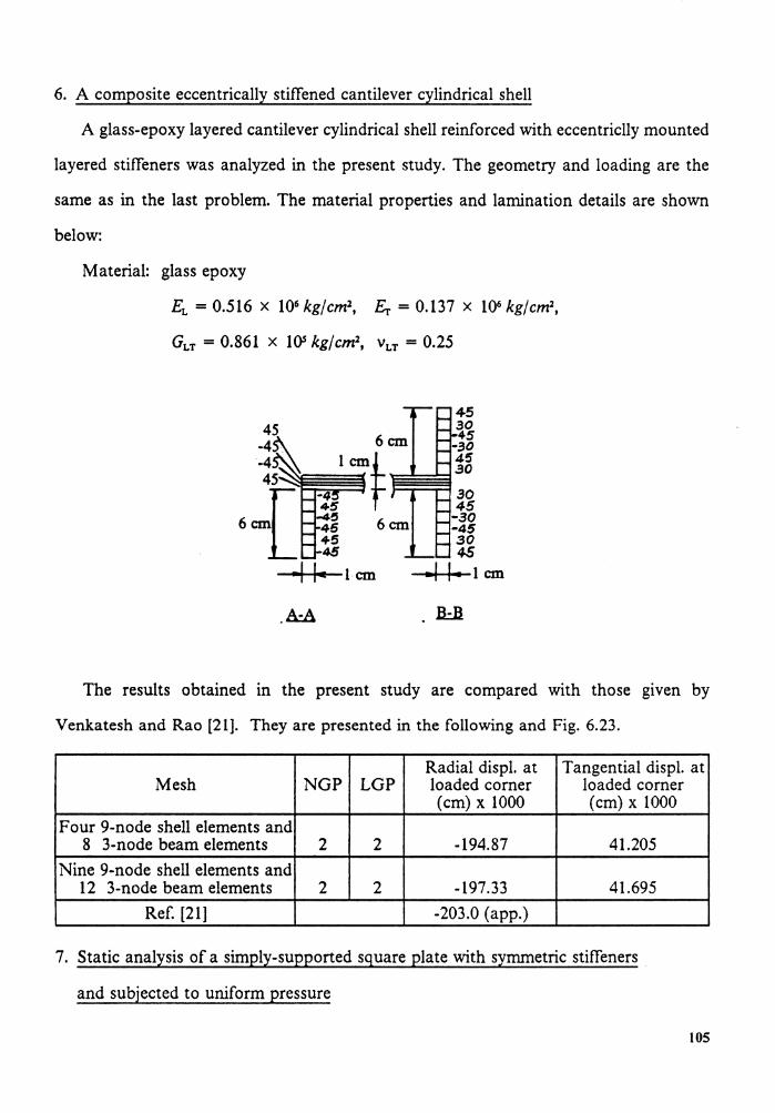
6. A composite eccentrically stiffened cantilever cylindrical shell
A glass-epoxy layered cantilever cylindrical shell reinforced with eccentriclly mounted
layered stiffeners was analyzed in the present study. The geometry and loading are the
same as in the last problem. The material properties and lamination details are shown
below:
Material: glass epoxy
EL = 0.516 x 10⁶ kg/cm2, Er = 0.137 x 10⁶ kg/cm2,
GLT = 0.861 x 10⁵ kg/cm2, vLT = 0.25
.A:A
The results obtained in the present study are compared with those given by
Venkatesh and Rao [21]. They are presented in the following and Fig. 6.23.
Radial displ. at Tangential displ. at Mesh NGP LGP loaded corner loaded corner
(cm) x 1000 (cm) x 1000 Four 9-node shell elements and
8 3-node beam elements 2 2 -194.87 41.205 Nine 9-node shell elements and
12 3-node beam elements 2 2 -197.33 41.695 Ref. [21) -203.0 (app.)
7. Static analysis of a simply-supported square plate with symmetric stiffeners .
and subjected to uniform pressure
105
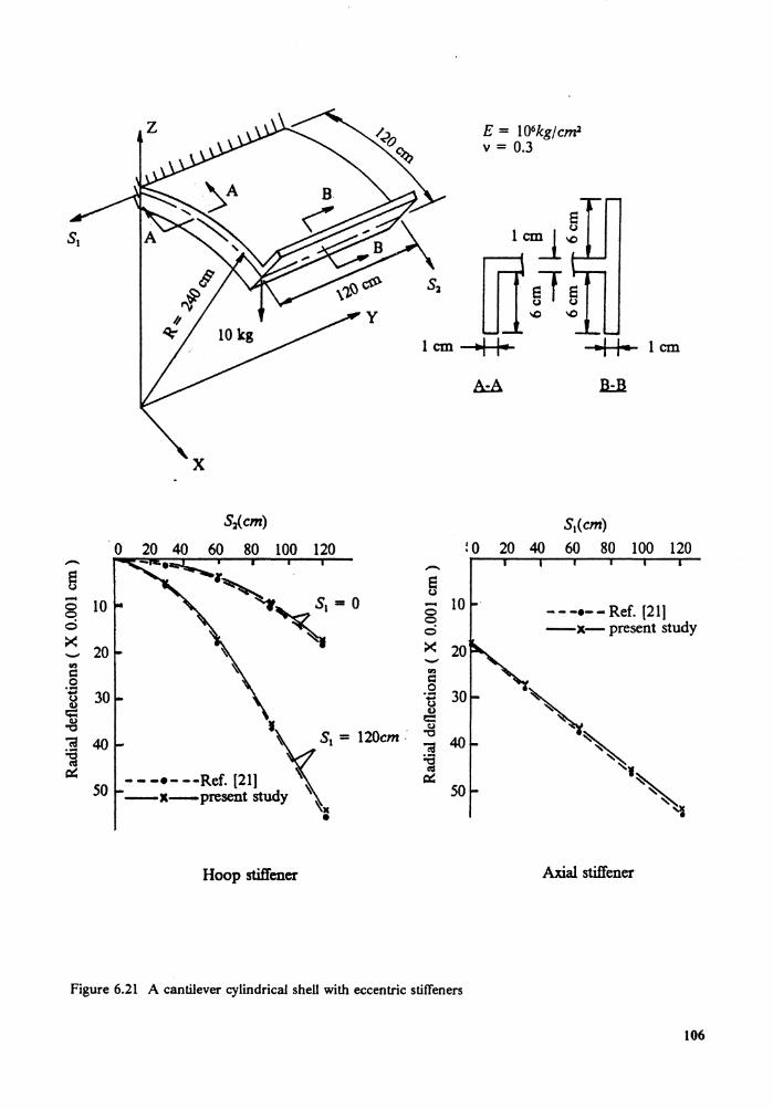
S,(cm)
0 20 40 60 80 100 120 -~ ,~ - 10 "'"< = 0
0 0 ci ~
20 -Ge = 0 ·;::: 30 () 0 = Q) :< . "'O
S1 = 120cm · ";! 40 ~ ex: - - -•---Ref. [21) ~ so -x-present study ~~.
•
Hoop stiffener
-e () -0
0 ci ~ -Ge = .9 ... () 0 = <:)
"'O ";! :e cu ex:
E = l06kg/cml v = 0.3
5 lcmj-o
rrr E1 E UJ \0 \0
~1 I• 1 cm
S1(cm) !O 20 40 60 80 100 120
10 ---•--Ref. (21) -x-present study
20
30
~, 40
"• ' so 'l
Axial stiffener
Figure 6.21 A cantilever cylindrical shell with eccentric stiffeners
106
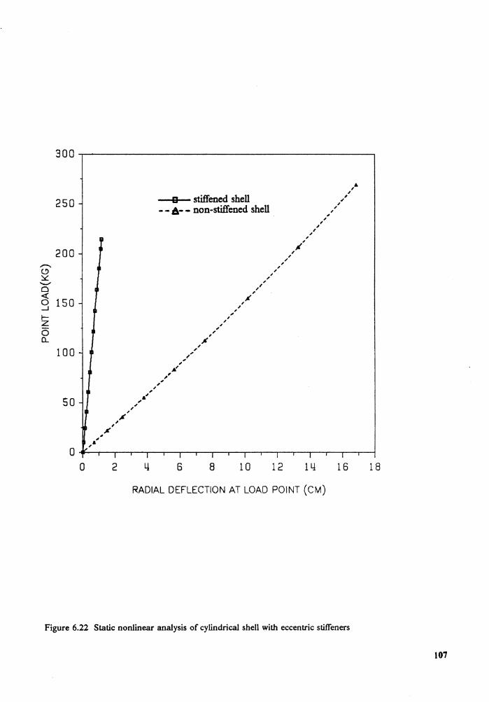
....-. 0 :::ii::: ......... 0 <( 0 _J
t-z 0 0..
250
200
150
100
so
B stiffened shell - - A- - non-stiffened shell
, , , ,
""' , ,
, , , , ,
, ~
, , ,/
, , ,
, , , , Jf'
, , , ,
, , , , , " ,
, , .. ,
0 -----r-~~~---r-~~~~~~~~~~~~~~~~~~---0 2 4 6 8 10 12 14 16 18
RADIAL DEFLECTION AT LOAD POINT (CM)
Figure 6.22 Static nonlinear analysis of cylindrical shell with eccentric stiffeners
107
30 60 90 120
---•--Ref. (21) -x-present study
Radial displacement of the hoop stiffeners
Figure 6.23 A cantilever composite cylindrical shell with eccentric stiffeners
108
The geometry of the stiffened plate is shown in Fig. 6.24. The material properties are:
E = 30 x 106 psi, v = 0.3, p = 2.5393 x 10- 4 !bf ~sec2
Due to symmetry, only one quarter of the stiffened plate was modelled with four 9-node
shell elements and eight 3-node beam elements. The geometric nonlinear responses of
this stiffened plate and the same plate without stiffeners are shown in the Fig. 6.24. The
same non-stiffened plate was analyzed also in Ref. [14] and the present results are close
to that in Ref. [ 14]. The effect of stiffeners on the response of the plate can be seen from
Fig. 6.24. The linear solutions for this stiffened plate are also included in the figure and
we can see that the stiffened plate in this case exhibits high geometric nonlinearity.
8. Static analysis of a simply-supported spherical shell with symmetric stiffeners
The geometry of the stiffened spherical shell is shown in Fig. 6.25. The material
properties are:
E 11\4 • 0 3 p = 2.3763 x 10-s !bf - sec2 · = v · psi, v = . , bt
Due to symmetry, only one quarter of the stiffened shell was modelled with sixteen
4-node shell elements and sixteen 2-node beam elements. The geometric nonlinear re-
sponses of this stiffened shell and the same shell without stiffeners (and subjected to a
center point load) are shown in Fig. 6.25. The same non-stiffened shell was analyzed by
Bathe and Ho [57] who used flat 3-node triangular shell element which includes trans-
verse shear deformation. The stiffened shell buckles under a center point load. The effect
of stiffeners on the the response of the shell can be seen from the figure.
9. Static analyses of 2-layer cross-ply and angle-ply simply-supported stiffened
laminated plates
The geometries of the two stiffened laminated plates and the associated stacking se-
quences are shown in Figures 6.26 and 6.27. The material properties used are:
Ex/ E, = 25, E, = 7.031 x 10⁵ N/cm2 , vx, = 0.25, Gx,/ E, = 0.5,
Gx% = Gxy• G,J E, = 0.2, p = 2.547 X I0- 6 ~:;c2
109
1. ..1 a
a= 40', h=0.2', E = 30 x 1·
106 psi, v = 0.3
o.2L~m I ' -I~-:::::::1::i: 0.2· 0.2"fWJ
1"
260.-~~~~~~~~~~~~~~~~~~~~
240
220 a stiffened plate ..
"I~ ~~ 200
. --~--A-::.·: nori~stlffened plate • Chang [14) -·. ~~·~-~·· ..... ···~·~·· -- -- -- ··-·- ·:i_-··-
II IQ.. 180
~ 160 ~ ~ lYO ~ ~ 1 2 0 -------------0 (§ 100 _J
8 0 -····-----·-·----···---···-·-·--··-···---·-·---
60
YO-+-----
20 +-------~~~
1
i .... -1-· l (__ ___ ---·-· i i
a ...... c;:::.:_,.~~r--+.--+---rL---r..:.........,~..-L-....--1--r-1---.-l-i......-1---,;~J,.._~ o . o o . 2 o . 4 a . s o . s 1 . o 1 . 2 i. 4 <1 . s 1 1 . s
WC/H
Figure 6.24 Static analysis of a simply-supported square plate with symmetric stiffeners and under
uniform pressure
110
z u = v = w = 01 = 03 = o
R= lOOn, a= 30.9017·, h= 3.9154" E = 104 psi, v = 0.3
u = v = w = 02 = 03 = 0 z u = 01 = 03 = 0 /"'F:::;~;i_
0 0 0
x ,--.. (/) co _J
........... 0 <{ 0 _J
15
10
5
a stiffened shell - - ~ - - non-stiffened shell ,.
I I
I I
I I
I I I
I I
I I
I I • ,,x-1r-,.,. .... , ,'
,A 'a ,' J{ ', I , ~ ,
{ ' , I '•-.-.,,,«
I .&
I I
I .. I
I I ,.
I
' I
f
a ...... ---.----.---.---..----.---...---r---r-----r---.---.-__,.---,..----.----.--i
0.0 0.5 1. 0 1. s 2.0 2.5 3.0 3. s 4.0
WC/H
Figure 6.25 Static analysis of a simply-supported spherical shell with symmetric stiffeners and under a
center point load
111
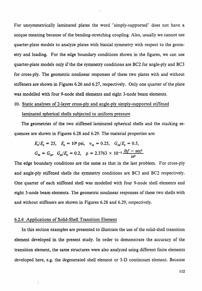
For unsymmetrically laminated plates the word "simply-supported" does not have a
unique meaning because of the bending-stretching coupling. Also, usually we cannot use
quarter-plate models to analyze plates with biaxial symmetry with respect to the geom-
etry and loading. For the edge boundary conditions shown in the figures, we can use
quarter-plate models only if the the symmetry conditions are BC2 for angle-ply and BC3
for cross-ply. The geometric nonlinear responses of these two plates with and without
stiffeners are shown in Figures 6.26 and 6.27, respectively. Only one quarter of the plate
was modelled with four 9-node shell elements and eight 3-node beam elements.
10. Static analyses of 2-layer cross-ply and angle-ply simply-supported stiffened
laminated spherical shells subjected to uniform pressure
The geometries of the two stiffened laminated spherical shells and the stacking se-
quences are shown in Figures 6.28 and 6.29. The material properties are:
EJ E, = 25, E, = 106 psi, v%, = 0.25, G%,/ E, = 0.5, _ _ _ _ 5 lb( - sec2
Gu - G%1 , G,J E, - 0.2, p - 2.3763 x 10 irt-
The edge boundary conditions are the same as that in the last problem. For cross-ply
and angle-ply stiffened shells the symmetry conditions are BC3 and BC2 respectively.
One quarter of each stiffened shell was modelled with four 9-node shell elements and
eight 3-node beam elements. The geometric nonlinear responses of these two shells with
and without stiffeners are shown in Figures 6.28 and 6.29, respectively.
6.2.4 Applications of Solid-Shell Transition Element
In this section examples are presented to illustrate the use of the solid-shell transition
element developed in the present study. In order to demonstrate the accuracy of the
transition element, the same structures were also analyzed using different finite elements
developed here, e.g. the degenerated shell element or 3-D continuum element. Because
112
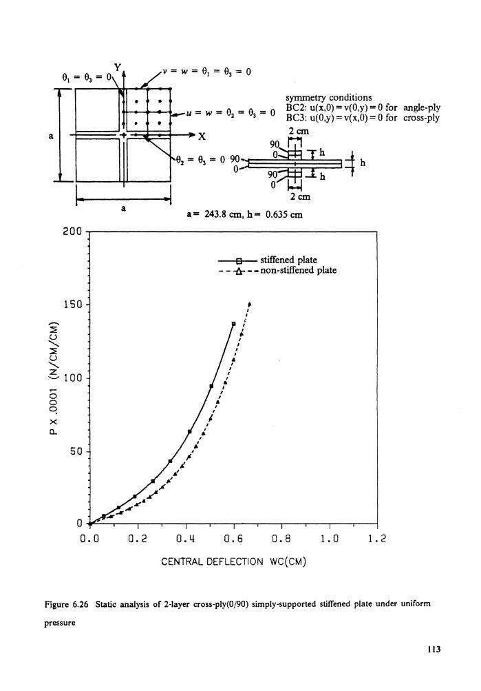
a
0 0 0
x Q...
I- a
150
50
symmetry conditions BC2: u(x,O) = v(O,y) = 0 for angle-ply BC3: u(O,y) = v(x,O) = 0 for cross-ply 2cm
9~1.1 02 = 03 = o 9g;::'1E=0:::::t::=-I=h31 -f. h 90jh i o~
2cm
a= 243.8 cm, h = 0.635 cm
I A
a stiffened plate - - -tr - - non-stiffened plate
.. I
I I
I I ,.
I
' I I
A I
I I
I • I I
I A
0 -'1F-'---.----.----.----.----.----.----.----.-----.-----.-----.----1
0.0 0.2 0.4 0.6 0.8 1. 0 1. 2
CENTRAL DEFLECTION WC(CM)
Figure 6.26 Static analysis of 2-layer cross·ply(0/90) simply-supported stiffened plate under uniform
pressure
113
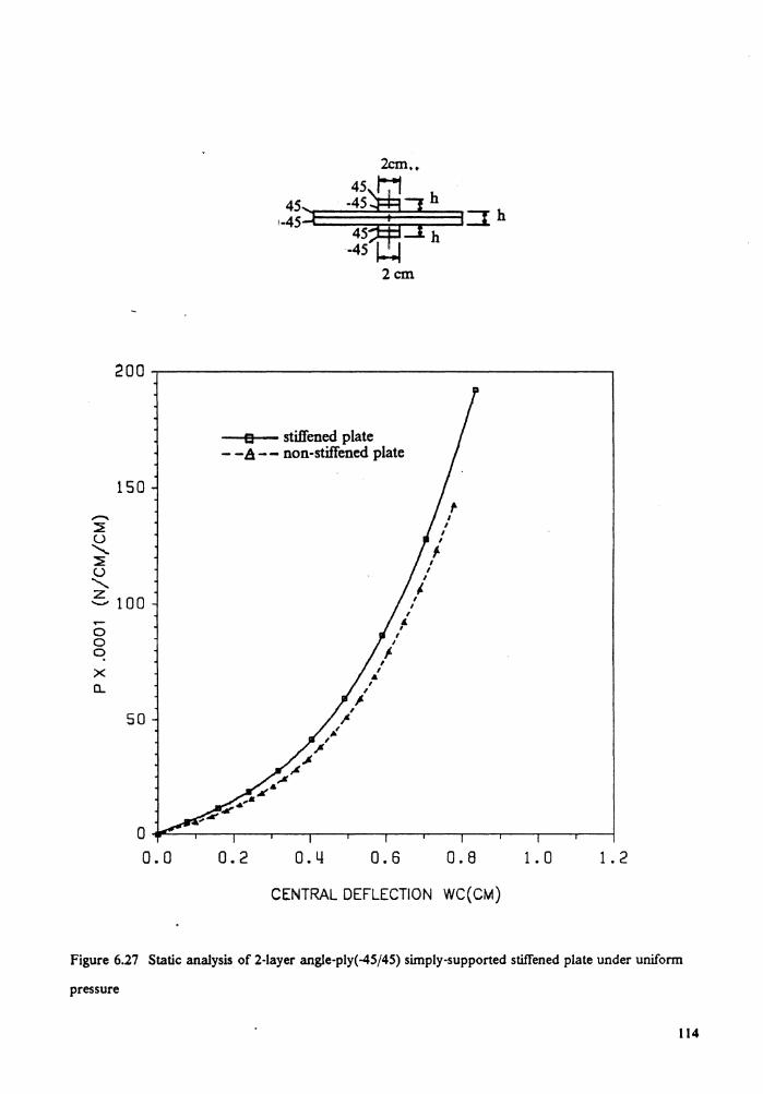
0 0 0
x CL
e stiffened plate - -6-- non-stiffened plate
150
50
0 ~:__...,...-~-.-~-.-~-.-~-.-~-.-~-.-~-.-~-.-~--,-~--,-~--!
0.0 0.2 0.4 0.6 0.8 1. 0 1. 2
CENTRAL DEFLECTION WC(CM)
Figure 6.27 Static analysis of 2-layer angle-ply(-45/45) simply-supported stiffened plate under uniform
pressure
114
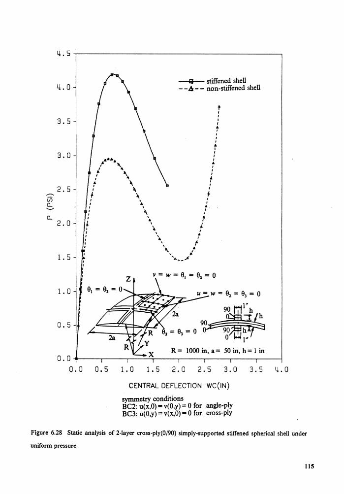
,.-... U5 0... ..._,,, 0...
4.0
3.5
3.0
2.5
2.0
1. 5
1. 0
0.5
I I I I
a stiffened shell - -.6- - non-stiffened shell
t I I I I • I
I I I • I
I I .... ~
f ~ I t "~ I : \ ~ . \ : II ~ I
+ ~ f I I I I I I I I • I
I I I I I
z
\ I •, A
~ ,' \ " A I
\ I
4 : \ A '. I
\ /' ~' /
'.,,_.If.
R= 1000 in, a= 50 in, h= 1 in 0.0-------.,..-----...-----.------.------r------..,.-----,..-----j
0.0 0.5 1. 0 1. 5 2.0 2.5 3.0
CENTRAL DEFLECTION WC(IN)
symmetry conditions BC2: u(x,O) = v(O,y) = 0 for angle-ply BC3: u(O,y) = v(x,O) = 0 for cross-ply
3.5 4.0
Figure 6.28 Static analysis of 2-layer cross-ply(0/90) simply-supported stiffened spherical shell under
uniform pressure
115
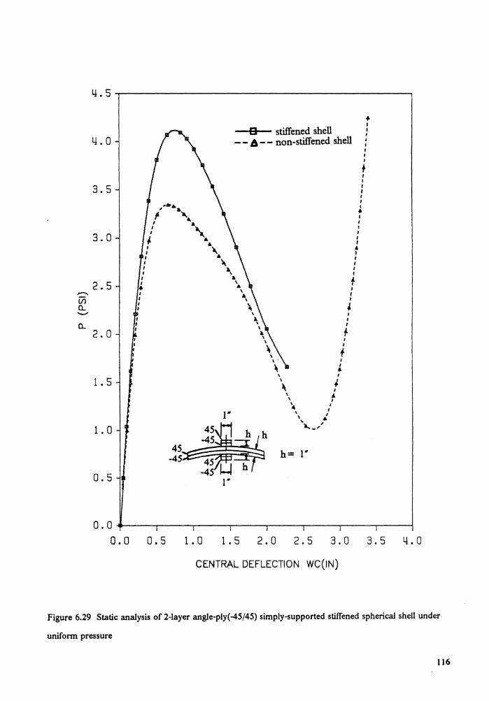
-. en a.. ........ a..
L!. 0
3.5
3.0
2.5
2.0
1. 5
1. 0
0.5
I I I I I I I I • I
I I I
I I I
,-··· ~ ' a
45 -45
'. a x.
\
B stiffened shell - - 6 - - non-stiffened shell
•,
+ I I I
' I I I I
+ I I I I I I I • I
I I I I I • I
I I I I a
\ a \
f
1·
", \
\ • ' \ a. \ \
\
I I I
l ' I
I
f I I
+ I I • \ I
\ ~ ~ I
\ " \ ' ~\ /
' . ~-,'
h= 1·
0.0+-~~.--~-.-~~-.-~~......-~~~~~~~~~-----1
o.o 0.5 1. 0 1. 5 2.0 2.5 3.0 3.5 4.0
CENTRAL DEFLECTION WC(IN)
Figure 6.29 Static analysis of 2-layer angle-ply(-45/45) simply-supported stiffened spherical shell under
uniform pressure
116
the transition element accounts for the transverse shear deformations, reduced inte-
gration was used to evaluate the transverse shear terms.
1. A cantilever plate
The plate and the four finite element models used are shown in Fig. 6.30. For the
bending loading of P = 30 lb/in at the free end, the lateral deflections w at x = 2 in, 4 in,
6 in and 8 in are:
0.011280 in, 0.040992 in, 0.082992 in, 0.13114in for model A
0.011283 in, 0.040998 in, 0.083002 in, 0.13115 in for model B
0.011280 in, 0.040992 in, 0.082995 in, 0.13114 in for model C
0.011283 in, 0.040998 in, 0.083002 in, 0.13115 in for model D
In this example problem we assume cr. = 0 and e. = 0 through the whole transition ele-
ment. The integration order for parabolic 3-D solid element and parabolic transition el-
ement is 3 x 3 x 2 for the bending part and 2 x 2 x 2 for the transverse shear part. I
For models B and D, since the normal stress cr. and the normal strain e. are neglected
through the whole plate, i.e. the stiffness in the transverse normal direction becomes
zero, the deflections are expected to be larger as compared with models A and C. This
example demonstrates the accuracy of the transition element in the linear analysis and
it illustrates the manner in which the transition elements can be connected to 3-D solid
elements or with themselves. This example was also analyzed by Surana [50].
2. A simply-supported isotropic beam subjected to a center point load
This example is used to evaluate the performance of the solid-shell transition ele-
ments in geometric nonlinear analysis. The material properties are:
E = 3 x l01 psi v = 0 p = 2.5393 x 10- 4 lb(- sec2
' ' in4 Fig. 6.31 shows the simply-supported beam and the finite element models. In Fig 6.3l(b)
the beam is modelled with three 11-node transition elements (back to back). Another
117
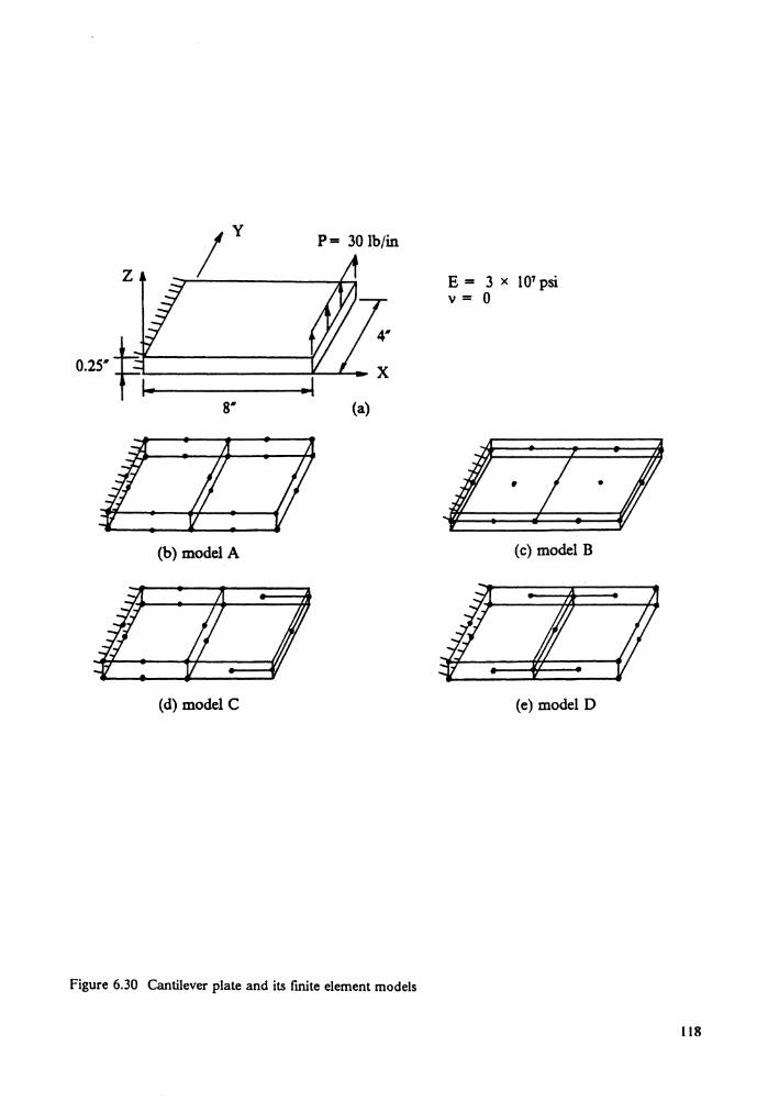
P= 30 lb/in
(a)
(b) model A
(d) model C
Figure 6.30 Cantilever plate and its finite element models
E = 3 x 10⁷ psi v = 0
(c) model B
(e) model D
118
finite element model using three 8-node degenerated shell elements is shown in Fig.
6.31(c). For linear analysis, when p= -0.6 lb, the center deflections are:
-0.0204815 in for the model with transition elements
-0.02048 m for classical beam theory
Fig. 6.32 shows plots of the load factor vs the central deflection ratio for these two
models and the results are almost the same. For the transition element model the de-
flections with cra ¢ 0 are less but very close to that with cra = 0. The effect of cra on the
performance of the transition element were investigated in details in Ref. [ 51 ].
3. A simply-supported 2-layer (0/90) beam subjected to a center point load
The same simply-supported beam as that in the last problem was used except that
the beam is composed of 2-layer (0/90) T300/5208 graphite-epoxy material. The material
properties are:
£1 = 19.2 x 10⁶ psi, ~ = E:i = 1.56 x 10⁶ psi, v12 = v13 = 0.24, v23 = 0.49,
G12 = G13 = 0.82 x 10⁶ psi, G 23 = 0.523 x 10⁶ psi, p = 2.3763 x 10-s lb{~ sec2
1n4 The two finite element models used in the last problem were used for the present prob-
lem. This example demonstrates the performance of solid-shell transition element used
in the composite plate analysis. Fig. 6.33 shows good agreement of the results of both
models in the geometric nonlinear analysis.
6.2.5 General Shell-Type Structures
I. A nonuniform cantilever plate
The plate considered consists of a short thick slab (2 in x 1 in x 0.7 in) and a very
thin long plate (10 in x 1 in x 0.1 in) joined together at the mid-plane as shown in Fig.
6.34(a). Two loading are applied respectively at the free end of the plate. Loading I is a
bending load of p= 3 lb/in and loading II is a inplane load of p= 120000 lb/in. Two
different models are used to model this structure. Model A in Fig. 6.34(b) contains ten
119
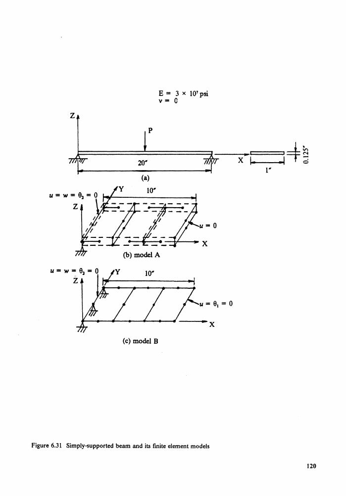
E = 3 x 10⁷ psi v = 0
z p
20"" x 1. ~=+=~ i •
(a)
10·
z
u=O
x (b) model A
10· ~1
u = 01 = 0
x (c) model B
Figure 6.31 Simply-supported beam and its finite element models
120
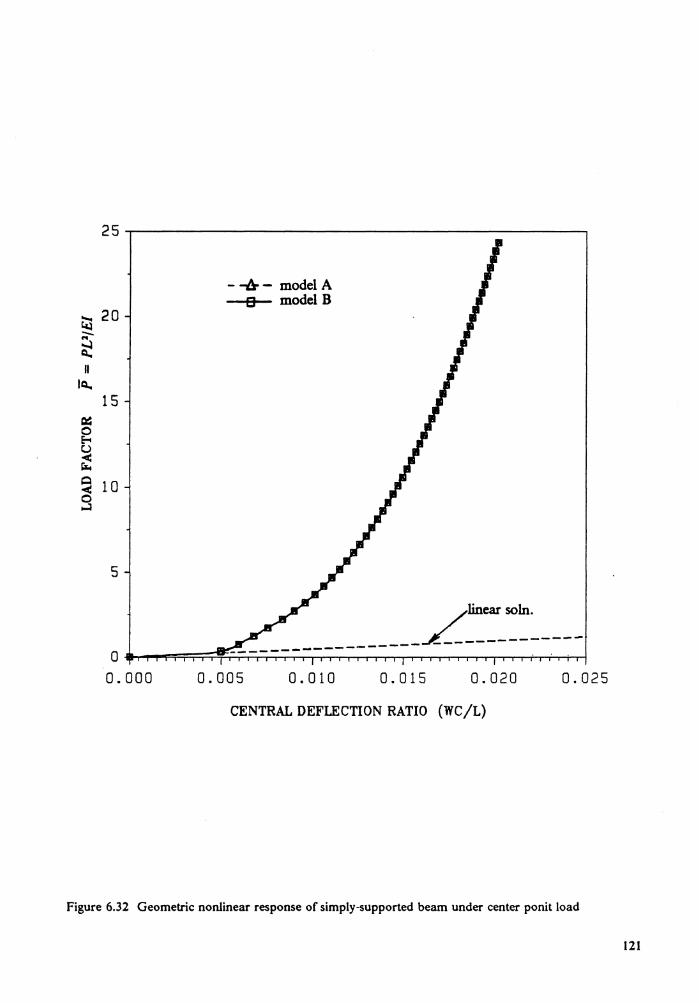
~ 20 -... ~ II
IQ.. 15
a:= 0 ~
~ Iii;. Q 10 < 0 ~
5
- -l!r - model A a model B
o..._~F'i"'r~~;:;:;=.::;.:~~-,--,--,-,--..-.--.~-,-,--..-.--.r--r-r--.-.-.,.-,-r--r-r-+-r--r-.--t-..1
0.000 0.005 0.010 0.015 0.020 0.025
CENTRAL DEFLECTION RATIO (WC/L)
Figure 6.32 Geometric nonlinear response of simply-supported beam under center ponit load
121
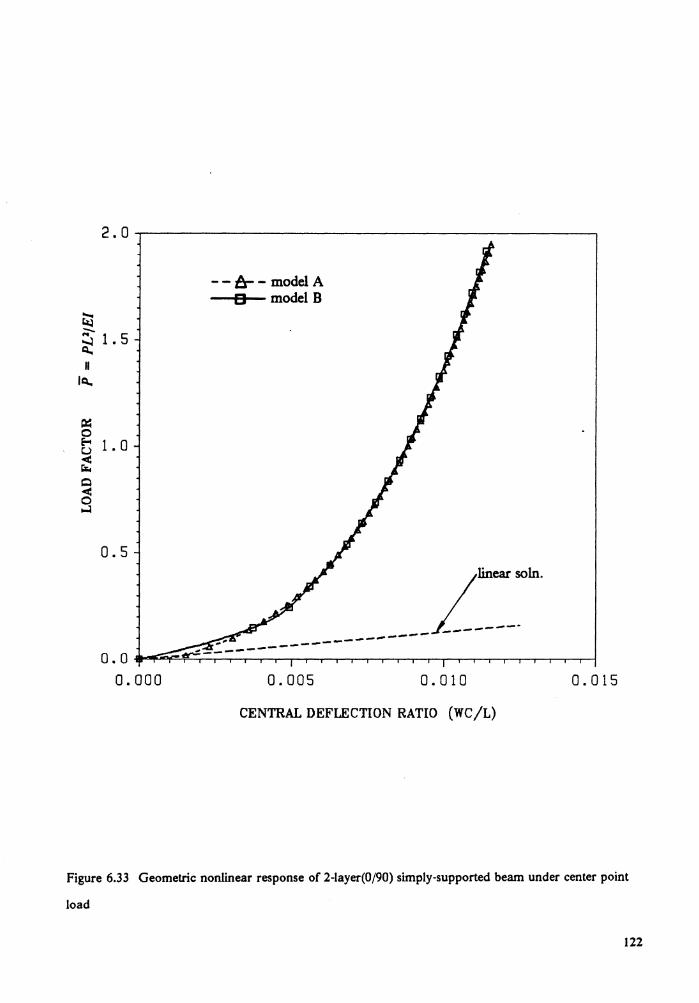
2.0
--&--model A B model B
~ ~ 1. 5 ~ II I~
Cl=: 0 e--. 1. 0 t..> < r:r. Q
~ ~
0.5
L:-~m. -----------------------0.0 ...... ~~~=-==--~~~~~~~~~~~~~~~~_J
0.000 0.005 0.010 0.015
CENTRAL DEFLECTION RATIO (WC/L)
Figure 6.33 Geometric nonlinear response of 2-layer(0/90) simply-supported beam under center point
load
122
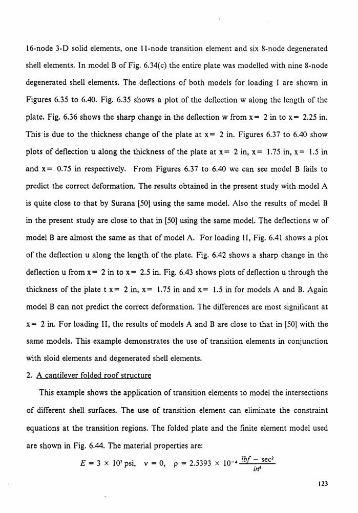
16-node 3-D solid elements, one 11-node transition element and six 8-node degenerated
shell elements. In model B of Fig. 6.34( c) the entire plate was modelled with nine 8-node
degenerated shell elements. The deflections of both models for loading I are shown in
Figures 6.35 to 6.40. Fig. 6.35 shows a plot of the deflection w along the length of the
plate. Fig. 6.36 shows the sharp change in the deflection w from x = 2 in to x = 2.25 in.
This is due to the thickness change of the plate at x = 2 in. Figures 6.37 to 6.40 show
plots of deflection u along the thickness of the plate at x= 2 in, x= 1.75 in, x= 1.5 in
and x= 0.75 in respectively. From Figures 6.37 to 6.40 we can see model B fails to
predict the correct deformation. The results obtained in the present study with model A
is quite close to that by Surana [50] using the same model. Also the results of model B
in the present study are close to that in [50] using the same model. The deflections w of
model B are almost the same as that of model A. For loading II, Fig. 6.41 shows a plot
of the deflection u along the length of the plate. Fig. 6.42 shows a sharp change in the
deflection u from x = 2 in to x = 2.5 in. Fig. 6.43 shows plots of deflection u through the
thickness of the plate t x= 2 in, x= 1.75 in and x= 1.5 in for models A and B. Again
model B can not predict the correct deformation. The differences are most significant at
x = 2 in. For loading II, the results of models A and B are close to that in [ 50] with the
same models. This example demonstrates the use of transition elements in conjunction
with sloid elements and degenerated shell elements.
2. A cantilever folded roof structure
This example shows the application of transition elements to model the intersections
of different shell surfaces. The use of transition element can eliminate the constraint
equations at the transition regions. The folded plate and the finite element model used
are shown in Fig. 6.44. The material properties are:
E = 3 x 10⁷ psi v = 0 p = 2.5393 x 10⁻⁴ lb[- sec2 f I in4
123
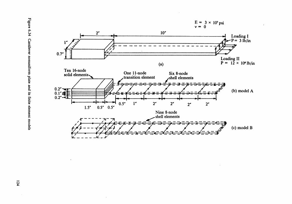
N .....
"T1 <iQ' c "' (D
C\ w "'" ~ C'.
f :;, 0 :;, c :;, ~ 3
"O iii" ~ Cl :;, 0. ~·
::ii :::3 ;-· ll. (D
3 g ... 3 0 0. ll. "'
E = 3 x 10⁷ psi v = 0
10· Loading I
2' - - - -- 4--p: Jib/in ·8_4------- -- -------- WC? 0.1·fr w :,-0_:diff ~1 IO'lb/in
Ten 16-node solid elements
(a)
Nine 8-node -f" - - - - - 71- 'I ~shell elements w. ·~z-·z:-z. z ~z_ -7
U.. - - -IL - _y - - - - - • •
(b) model A
(c) model B
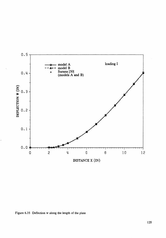
0.4
-z -......... 0 3 ~ . z 0 -E--o u ~ ~ 0.2 J:;;;i Q
0. 1
a model A - - A• - model B
• Surana [ 50) (models A and B)
loading I
o.o...-T"TT",..,...,r-T""T"~~~..,,....r-r-r,..,...,,.....,...,.,..,..,,....T""T""T..,,....r-T"T,..,...,,.....,...,.,..,.,,...T"TT",..,...,r-rr~
0 2 6 8 10 12
DISTANCE X (IN)
Figure 6.35 Deflection w along the length of the plate
125
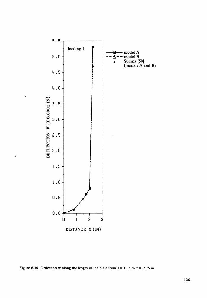
-z .... """ 0 0 0 0 >< .._.. ~
z 0 -~ t:.)
~ ~ ~ Q
5. 5 ........---------, loading I
5.0
4.5
LL 0
3.5
3.0
2.5
2.0
1. 5
1. 0
0 1 2 3
DISTANCE X (IN)
8 model A --A-- model B
• Surana (50) (models A and B)
Figure 6.36 Deflection w along the length of the plate from x = 0 in to x = 2.25 in
126
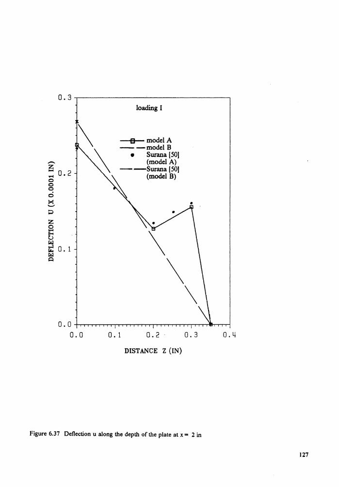
-z ::: 0.2 0 0 0 0 >< ......... 0 z 0 .... E-< C',)
~ 0. 1 r:.r:l Q
loading I
B modelA --modelB
• Surana ( 50] (model A)
- -Surana (50) (model B)
0 . 0 -1-.-~........,.....,..,.-..-.-.....,--,-...,..,.-T""T'""T-,-,-..,....,...T'""T"""""T-r-T""T""T""r-r-T-rTl!l!IT-rrr-1
0.0 0. 1 0.2 0.3 0.4
DISTANCE Z (IN)
Figure 6.37 Deflection u along the depth of the plate at x = 2 in
127
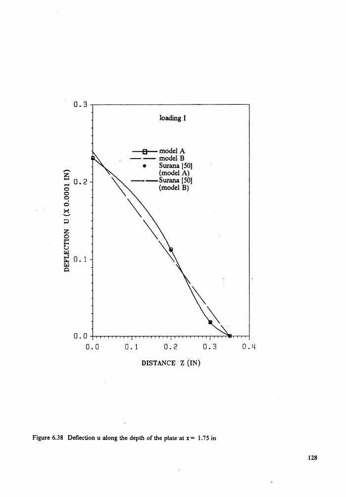
-z ::: 0.2 0 0 0 0 >< .._,. :,::;)
z 0 .... E--< t..>
~ 0. 1 r:..:l Q
loading I
8 model A -- modelB
• Surana [ 50) (model A)
\""- --Surana (50) '\ (model B)
\ ~ ~
0.0-1-.-~~~~~-.--.-~,.......-.,.-.--.-~..,--,--.--.-~r-r-T'llh-~
0.0 0. 1 0.2 0.3 0.4
DISTANCE Z (IN)
Figure 6.38 Deflection u along the depth of the plate at x = 1. 7 5 in
128
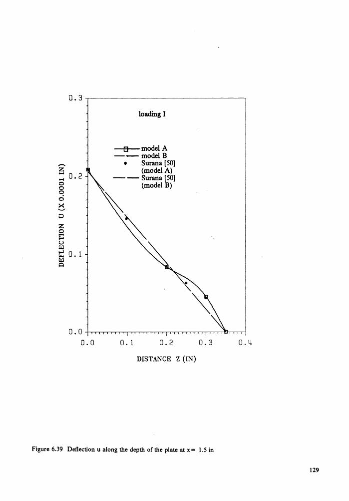
loading I
a model A --modelB - • Surana [50) z (model A) -0.2 --Surana [50) o-1
0 (model B) 0 0 0 >< ......., ::> z 0 -~ u ~ t: 0. 1 ~ Q
0.0-h-T""T"""T-rr-T""T""T-rr-T""T"T..,-,-TTT..,,-TTT..,,-rrTJT"rrT-err-rr; 0.0 0. 1 0.2 0.3 0.4
DISTANCE Z (IN)
Figure 6.39 Deflection u along the depth of the plate at x = LS in
129
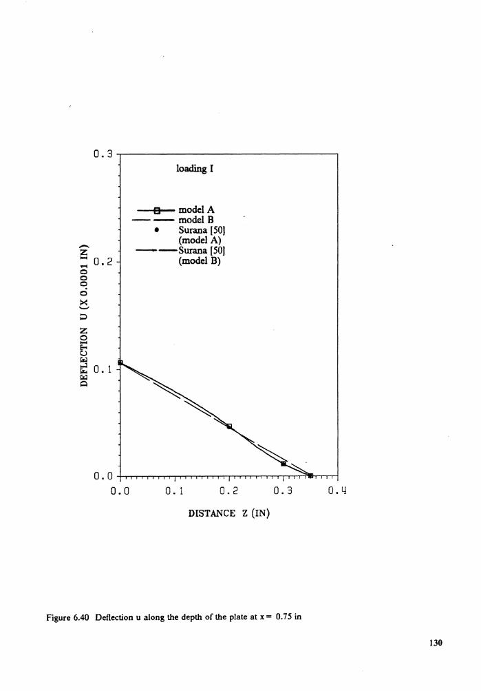
-z ::: 0.2 0 0 0 0 >< ...._.. ::> z 0 -E-< c:,,) w ~ 0. 1 w Q
loading I
8 model A ---modelB
• Surana (50) (model A)
--Surana (50) (model B)
O.O-+-r"T""T""",...,...........-.--r-r-,...,...........-.-T"T"""~.....-.-.,.......,.....,.-,--.-.-.,-,....,~...._..-,-,-
0.0 0. 1 0.2 0.3 0. 4
DISTANCE Z (IN)
Figure 6.40 Deflection u along the depth of the plate at x = 0. 7 5 in
130
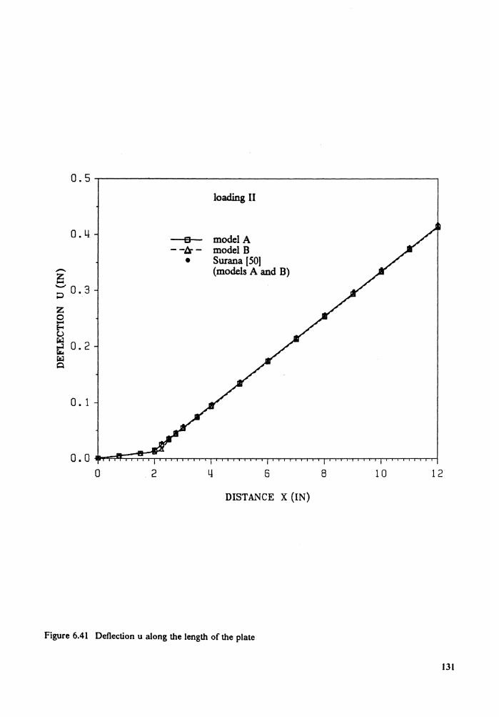
0.4
-i!i ';;' 0.3
z 0 .... Eo-< t.>
~ 0.2 rz:I Q
o. 1
o 2
loading II
a model A - -tr - model B
• Surana (50) (models A and B)
4 6
DISTANCE X (IN)
Figure 6.41 Deflection u along the length of the plate
8 10 12
131
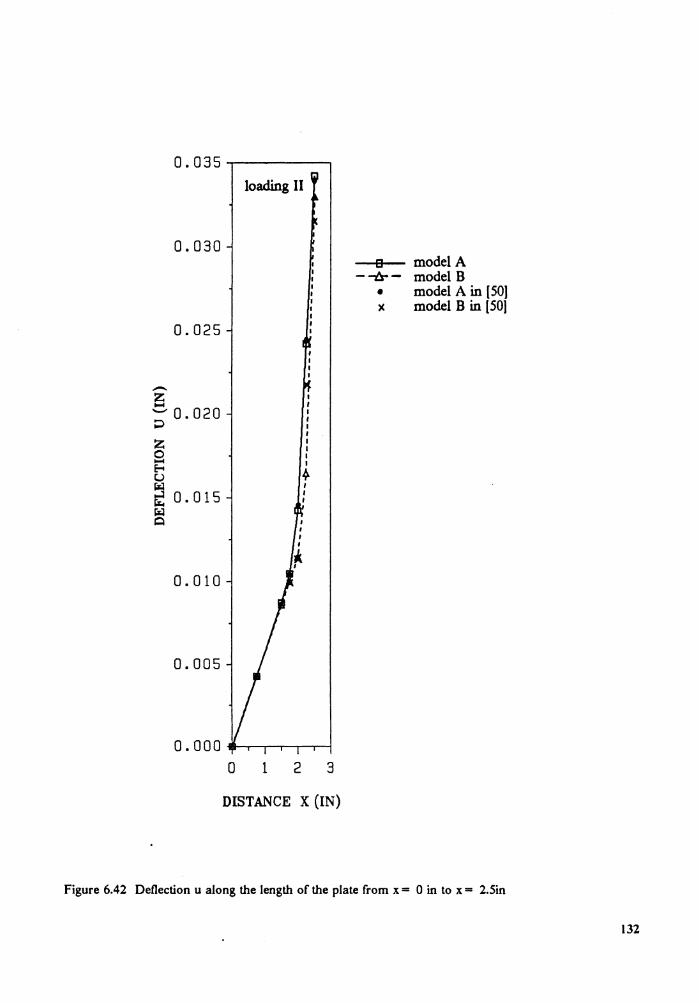
loading II
0.030 a model A
- -l:!r - model B • model A in [ 50) x model B in (50)
0.025
-z I .... I
; 0. 020 I I I I z I I 0 I .... I E-o ~ u
~ 0.015 r.;l Q I
I I
'
" I
0.010
0.005
0 • 0 0 0 -,........,..----.---r-...,--,
0 1 2 3
DISTANCE X (IN)
Figure 6.42 Deflection u along the length of the plate from x = 0 in to x = 2.5in
132
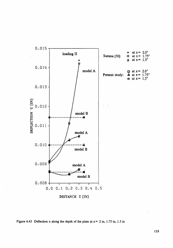
0.014
0.013
-z .... ;0.012 z 0 .... E--t..)
~ 0.011 ril Q
0.010
0.009
loading II
•
model A
model B
model B
model A
model B
0.008-+-~-.---~.,..--~~~.-----t
0.0 0.1 0.2 0.3 0.4 0.5
DISTANCE Z (IN)
• at x= 2.0 ... Surana (50): + at x= l.75n
X at x= 1.5 ...
o at x= 2.0" Present study: A at x= 1.75 ...
o at x= 1.5*
Figure 6.43 Deflection u along the depth of the plate at x = 2 in, 1. 75 in, 1.5 in
133
The predicted bending stresses of the folded roof in the present study are shown in Fig.
6.45, which are in good agreement with the results obtained with 2-D fine mesh by Bathe
and Ho [49]. With the same accuracy the model employing transition element has much
less degrees-of-freedom in analysis as compared with the 2-D model and does not need
the constraint equations at the transition regions. Large deformation analysis of this
folded plate was also performed here. The loading is the same. Fig. 6.46 shows the results
of geometric nonlinear analysis compared with the linear solution. In the load range
shown the roof does not exhibit high geometric nonlinearity.
3. A simply-supported beam with nonuniform thickness under a center point load
Figure 6.47 shows the geometry of the nonuniform beam and its finite element
models. The material properties are:
E = 3 x 10⁷ psi, v = 0, P = 2.5393 x 10⁻⁴ lb[ - secl bf
Static response of this beam is studied by using two finite element models. Model A in
Fig. 6.47(b) combines three 16-node solid elements, one 11-node solid-shell transition
element and one 8-node degenerated shell element. In model B of Fig. 6.47(c) we use
three 8-node shell elements. For linear analysis, when p= -0.6 lb the center deflections
are:
-0.010882 in for model A
-0.011791 in for model B
-0.011171 in for classical beam theory
The geometric nonlinear solutions of these two models are shown in Fig. 6.48. The
load-deflection curves of these two models are close to each other. From the results we
can see that this nonuniform simply-supported beam becomes stiffer as the loading in-
creases.
4. A layered composite simply-supported beam with nonuniform thickness
under a center point load
134
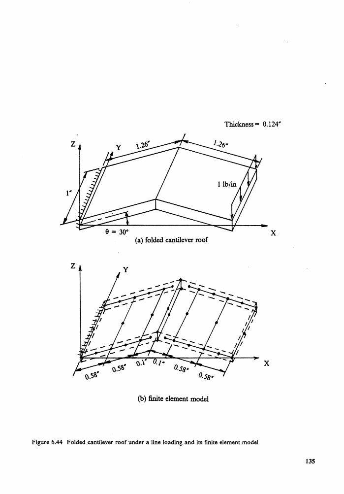
lbickness= 0.124 ...
x (a) folded cantilever roof
x
(b) finite element model
Figure 6.44 Folded cantilever roof under a line loading and its finite element model
135
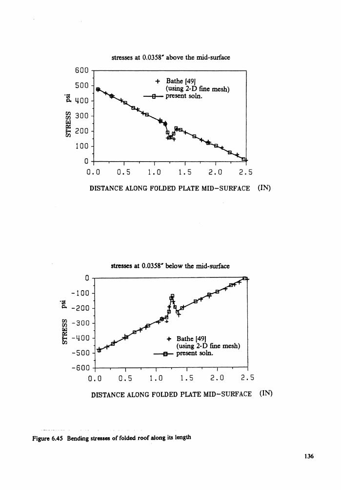
stresses at 0.0358' above the mid-surface
600
500 + Bathe [49) (using 2-D fine mesh) .... B present soln . So YOO
en 300 en l";i:J et: 200 E--o en
100
0 0.0 0.5 1. a 1. 5 2.0 2.5
DISTANCE ALONG FOLDED PLATE MID-SURFACE (IN)
stresses at 0.0358' below the mid-surface
0....--------------------------------n. -100
·~ Q. -200
~ -300 l";i:J et: ~ -400
-500
+ Bathe (49) (using 2-D fine mesh)
-""'B- present soln.
-600-+---.....--~--.----.----.---.---,..--.--..----i
a.a 0.5 1. a 1. 5 2.0 2.5
DISTANCE ALONG FOLDED PLATE MID-SURFACE (IN)
Figure 6.45 Bending stresses of folded roof along its length
136
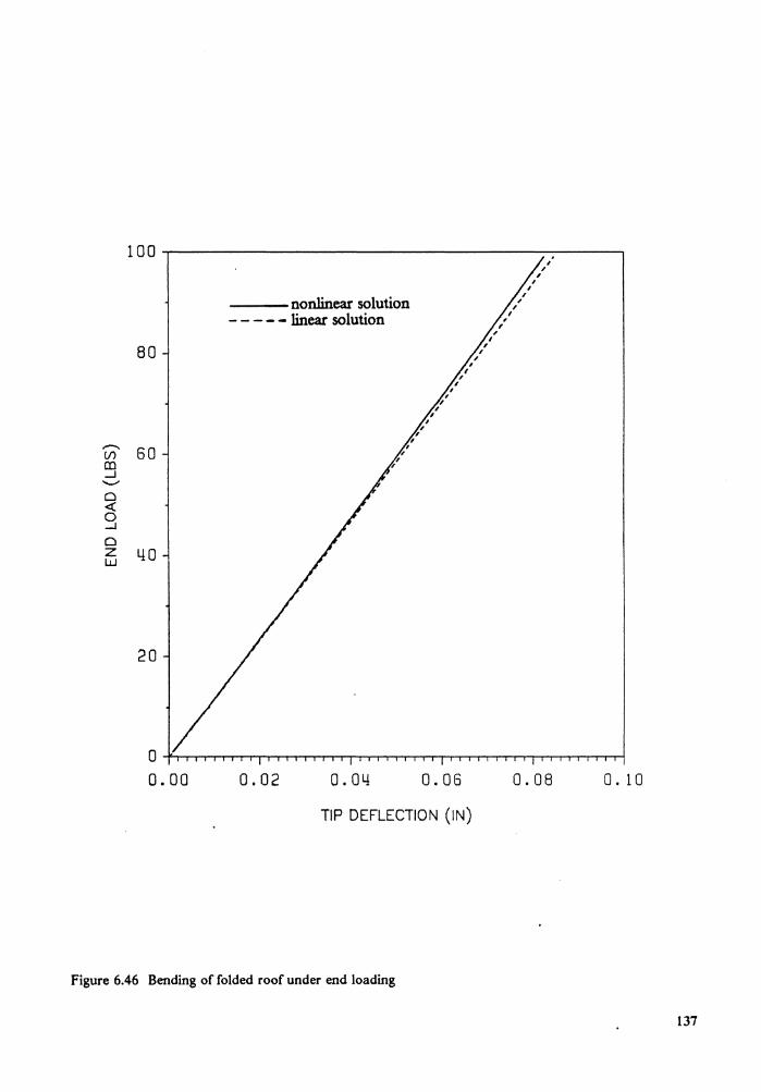
--.. (/) al _J .......,, 0 <( 0 _J
Cl z w
100--~~~~~~~~~~~~~~~~~~~~~
---nonlinear solution - - - - - linear solution ,
I , I , 80
60
40
20
, I
I , ,
, I
, , , ,
0 -l'--.-~~~...-.-.,..-,-.,....,....~~~~.-.-.~~~~~~~~...-.-.,..-,-~~T""""i 0.00 0.02 0.04 0.06 0.08 0. 10
TIP DEFLECTION (IN)
Figure 6.46 Bending of folded roof under end loading
137
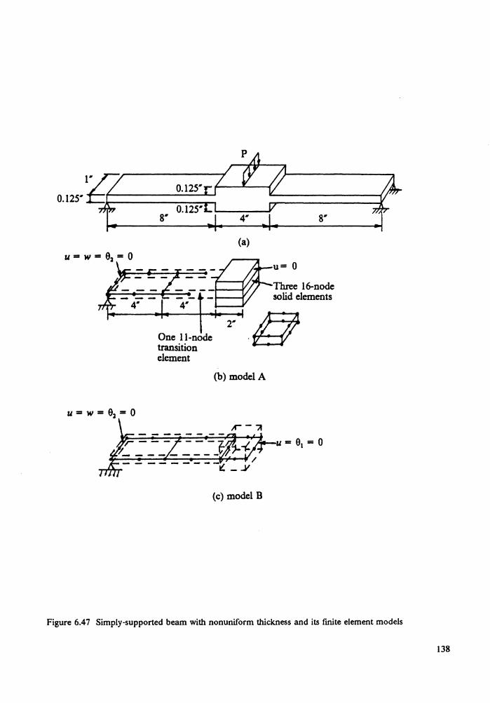
0.125· g 0.125.. :::::::::::::::::
u=w=01 =0
0.125·
One 11-node transition element
(a)
(b) model A
(c) model B
u = e1 = o
Figure 6.47 Simply-supported beam with nonuniform thickness and its finite element models
138
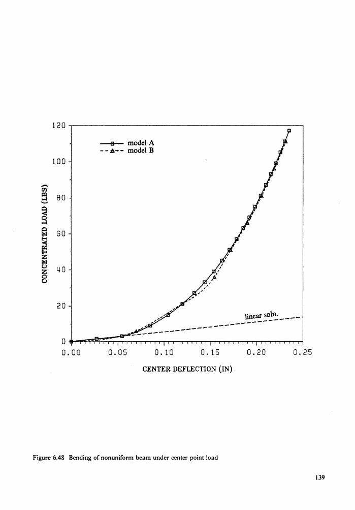
a model A - - 6-- model B
100
-r:n i:c 80 ~ -~ 0 ~
i:::i 60 ~
~ z ~ c..> 40 z 0 c..>
20 linear soln. -------------------------
o~~~~~,...,....,... ............ -.-.-.--.-.-,....,..........--.--r-r-r-.--.-.-.,.-,-,--.-......--.--r-"',...,....,....,........,.~ 0.00 0.05 0. 10 0. 15 0.20 0.25
CENTER DEFLECTION (IN)
Figure 6.48 Bending of nonuniform beam under center point load
139
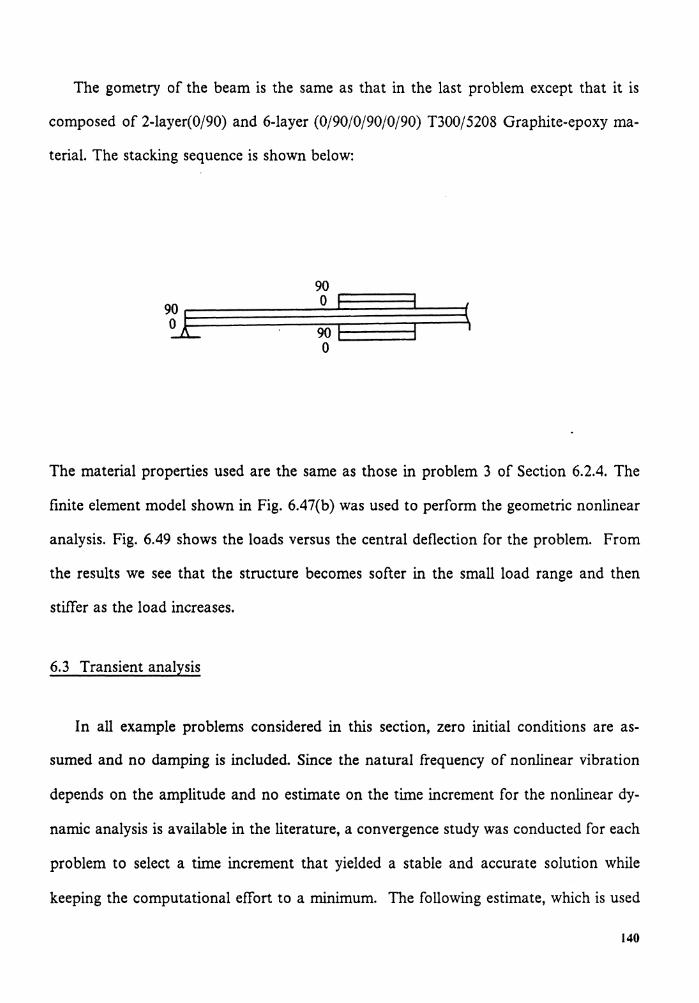
The gometry of the beam is the same as that in the last problem except that it is
composed of 2-layer(0/90) and 6-layer (0/90/0/90/0/90) T300/5208 Graphite-epoxy ma-
terial. The stacking sequence is shown below:
90 90~~~~~~~-o.:!~----~-:~4( ~ 90l 1
0
The material properties used are the same as those in problem 3 of Section 6.2.4. The
finite element model shown in Fig. 6.47(b) was used to perform the geometric nonlinear
analysis. Fig. 6.49 shows the loads versus the central deflection for the problem. From
the results we see that the structure becomes softer in the small load range and then
stiff er as the load increases.
6.3 Transient analysis
In all example problems considered in this section, zero initial conditions are as-
sumed and no damping is included. Since the natural frequency of nonlinear vibration
depends on the amplitude and no estimate on the time increment for the nonlinear dy-
namic analysis is available in the literature, a convergence study was conducted for each
problem to select a time increment that yielded a stable and accurate solution while
keeping the computational effort to a minimum. The following estimate, which is used
140
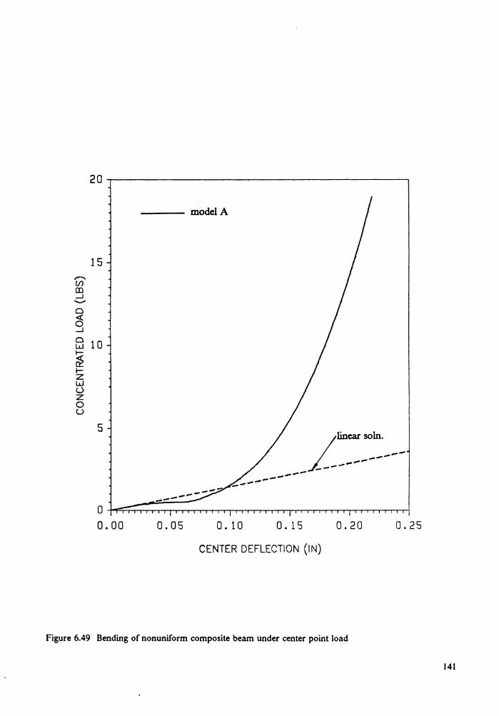
.,,-... (/) CD ......J ........... 0 ~ ......J 0 w
~ I-z w (.) z 0 u
---- modelA
15
10
5
------ ----/
linear soln. --
~-----_ ... ---
0 -l-oF::;;::.......-.-..,.....,.....,.....,.....--.-..--.-..-..-..-..-..-..-r-..-r-r-ir-r-1-r-T"""T""'T-r-T"-r-T"-r-T"""T""T"..,.....,..."'T""T'""'T""T'"T""T""r-rrl
0.00 0.05 0. 10 0. 15 0.20 0.25
CENTER DEFLECTION (IN)
Figure 6.49 Bending of nonuniform composite beam under center point load
141
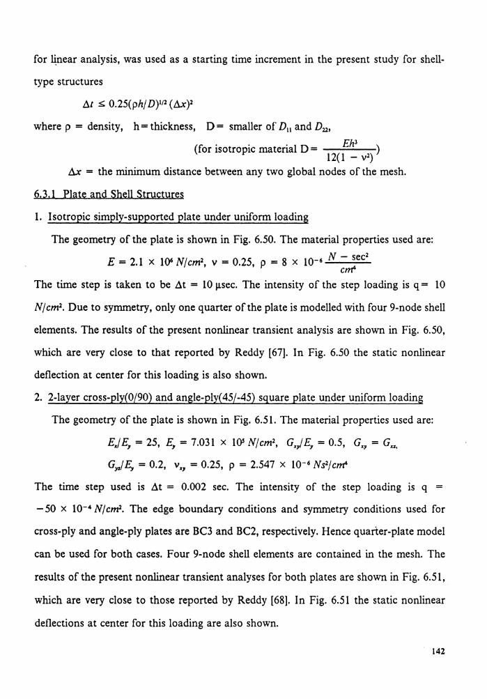
for li:near analysis, was used as a starting time increment in the present study for shell-
type structures
~t ~ 0.25(ph/ D)112 (Ax)2
where p = density, h =thickness, D = smaller of D11 and D22,
( t'. • • • 1 D Ehl ) 1or isotropic matena = ----12( 1 - v2)
Ax = the minimum distance between any two global nodes of the mesh.
6.3.1 Plate and Shell Structures
1. Isotropic simply-supported plate under uniform loading
The geometry of the plate is shown in Fig. 6.50. The material properties used are:
E = 2.1 x 10⁶ N/cm2, v = 0.25, p = 8 x 10⁻⁶ N ;,;ec2
The time step is taken to be ~t = 10 µsec. The intensity of the step loading is q = 10
N/cm2• Due to symmetry, only one quarter of the plate is modelled with four 9-node shell
elements. The results of the present nonlinear transient analysis are shown in Fig. 6.50,
which are very close to that reported by Reddy [67]. In Fig. 6.50 the static nonlinear
deflection at center for this loading is also shown.
2. 2-layer cross-ply(0/90) and angle-ply( 45/-45) square plate under uniform loading
The geometry of the plate is shown in Fig. 6.51. The material properties used are:
E,JE, = 25, E, = 7.031 x 10⁵ N/cm2, Gz,/E, = 0.5, Gz, = Gu,
G,J E, = 0.2, vz, = 0.25, p = 2.547 x 10⁻⁶ Ns2/crrt
The time step used is ~t = 0.002 sec. The intensity of the step loading is q = -50 x 10-4 N/cm2• The edge boundary conditions and symmetry conditions used for
cross-ply and angle-ply plates are BC3 and BC2, respectively. Hence quarter-plate model
can be used for both cases. Four 9-node shell elements are contained in the mesh. The
results of the present nonlinear transient analyses for both plates are shown in Fig. 6.51,
which are very close to those reported by Reddy (68]. In Fig. 6.51 the static nonlinear
deflections at center for this loading are also shown.
142
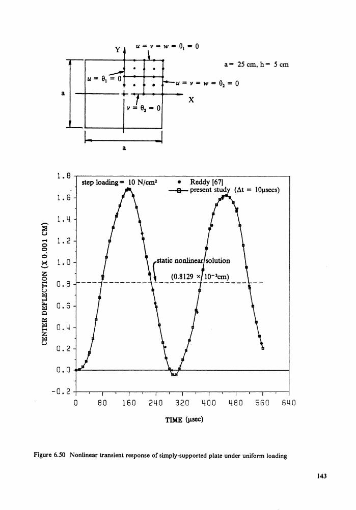
~
0 0 0 >< ......,
y u = v = w = 01 = o
• • a= 25 cm, h= S cm
• • a -~---~ -.. ....... _ ....... __
x
1. a
1.8...-~~~~~~~~~~~~~~~~~~~~---,
step loading= 10 N/cm.2 • Reddy (67] --a-present study (.M = lOµsecs)
1. 6
1. 4
1. 2
1. 0
0.8
0.6
0.4
0.2
-0.2+--.-~.---r--,..~~-.---r~~-r---,;---r----r~r---.--.----i
0 80 160 240 320 400
TIME (µsec)
480 560 640
Figure 6.50 Nonlinear transient response of simply-supported plate under uniform loading
143
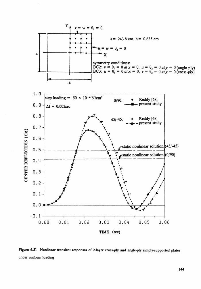
-::e t.) ..._, z 0 -Ee-t.)
:3 r:.:.. ~ ~
c:: ~ Ee-z ~ t.)
a
y v = w = 01 = o
• • a= 243.8 cm, h = 0.635 cm
• • = w = 02 = 0 ---!~--- + _____ ......, __ x
symmetry conditions: BC2: v = 01 = 0 at x = 0, u = 02 = 0 at y = 0 (angle-ply) ........ ----+----~ BC3: u = 01 = 0 at x = 0, v = 02 = 0 aty = 0 (cross-ply)
·' a
step loading == SO x 10-4 N/cm.2
0 • 9 At = 0.002sec 0/90: • Reddy [68)
--ta- present study
0.8
0.7
0.6
0.5
o. 4
0.3
0.2
o. 1
0.0
-0. 1
45/-45: + Reddy [68) - + - present study
' \ 't
\ \
\
\ rstatic nonlinear solution ( 45/-45)
- ~(static ~onlinear solution (0/90) --- I - -
\ \ \
~+
I I
,4
I I
I • I
0.00 0. 01 0.02 0.03 0.04 0.05 0.06
TIME (sec)
Figure 6.51 Nonlinear transient responses of 2-layer cross-ply and angle-ply simply-supported plates
under uniform loading
144
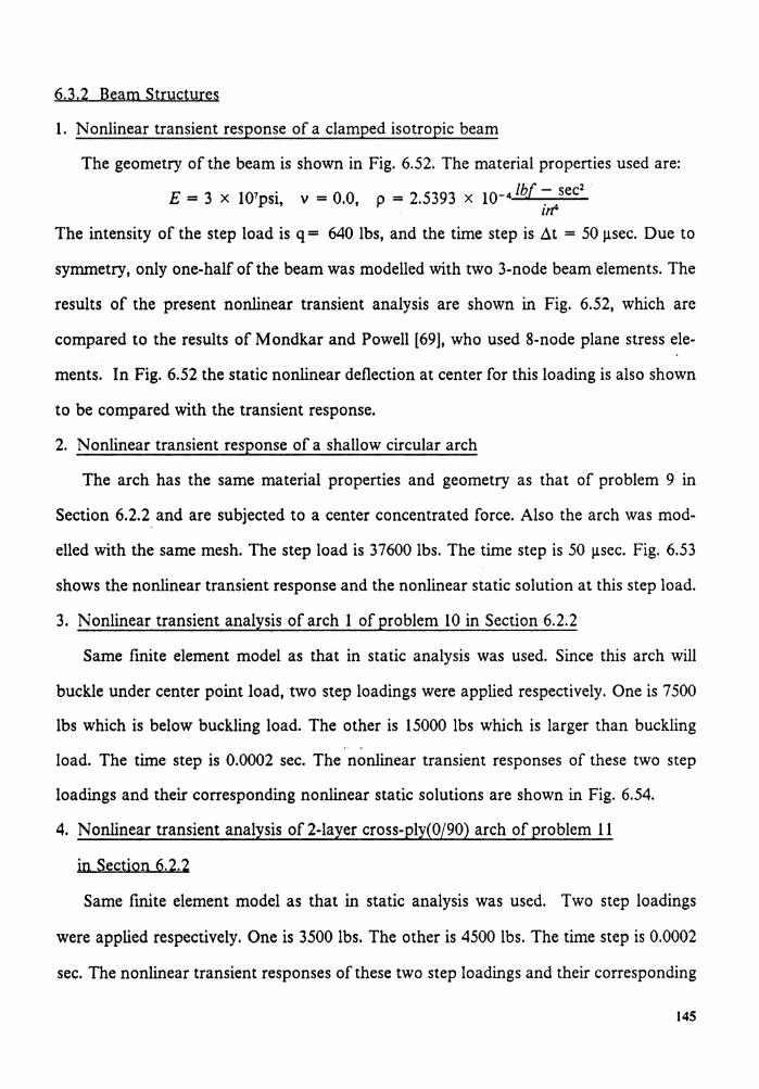
6.3.2 Beam Structures
l. Nonlinear transient response of a clamped isotropic beam
The geometry of the beam is shown in Fig. 6.52. The material properties used are:
E = 3 x l01psi, v = 0.0, p = 2.5393 x 10- 4 lb( ~sec2 . l
The intensity of the step load is q = 640 lbs, and the time step is .!lt = 50 µsec. Due to
symmetry, only one-half of the beam was modelled with two 3-node beam elements. The
results of the present nonlinear transient analysis are shown in Fig. 6.52, which are
compared to the results of Mondkar and Powell [69), who used 8-node plane stress ele-
ments. In Fig. 6.52 the static nonlinear deflection at center for this loading is also shown
to be compared with the transient response.
2. Nonlinear transient response of a shallow circular arch
The arch has the same material properties and geometry as that of problem 9 in
Section 6.2.2 and are subjected to a center concentrated force. Also the arch was mod-
elled with the same mesh. The step load is 37600 lbs. The time step is 50 µsec. Fig. 6.53
shows the nonlinear transient response and the nonlinear static solution at this step load.
3. Nonlinear transient analysis of arch 1 of problem 10 in Section 6.2.2
Same finite element model as that in static analysis was used. Since this arch will
buckle under center point load, two step loadings were applied respectively. One is 7500
lbs which is below buckling load. The other is 15000 lbs which is larger than buckling
load. The time step is 0.0002 sec. The nonlinear transient responses of these two step
loadings and their corresponding nonlinear static solutions are shown in Fig. 6.54.
4. Nonlinear transient analysis of 2-layer cross-ply(0/90) arch of problem 11
in Section 6.2.2
Same finite element model as that in static analysis was used. Two step loadings
were applied respectively. One is 3500 lbs. The other is 4500 lbs. The time step is 0.0002
sec. The nonlinear transient responses of these two step loadings and their corresponding
145
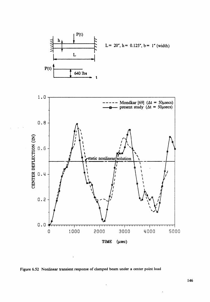
~ bl 1 ..
P(t) l
0.8
z 0 0.6 E=: u
~ ~ 0
~ 0.4 E-< z ~ u
0.2
t
l P(t)
L
640 lbs
\ I
~ ·I
... t
L= 20·, h= 0.125', b= 1· (width)
- - - - - Mondkar [69) (Llt = 50µsecs) a present study (Llt = 50µsecs)
\ ' ·---fstatic no~ear solu~o_n __ '-\-\ I I \ \ I I I I I
\
0.0 ....... ..,...,....,...,....,,....,...,.--r-r..,....,....,...,....,....,....,""T""T-.--.-~...-.-~~~~~~~~..,...,....~---l 0 1000 2000 3000 4000 5000
TIME (µsec)
Figure 6.52 Nonlinear transient response of clamped beam under a center point load
146
10 (at = 50µsecs)
9 step center load= 37600 lbs
8
- 7 ~ .._, z 6 0 -~ t.> ~ 5 l:';i;. r:.:l Q static nonlinear solution e::: L! r:.:l ~ z r:.:l 3 t.>
2
1
0 0 1000 2000 3000 l.!000 5000
TIME (µsec)
Figure 6.53 Nonlinear transient response of shallow circular arch under a center point load
147
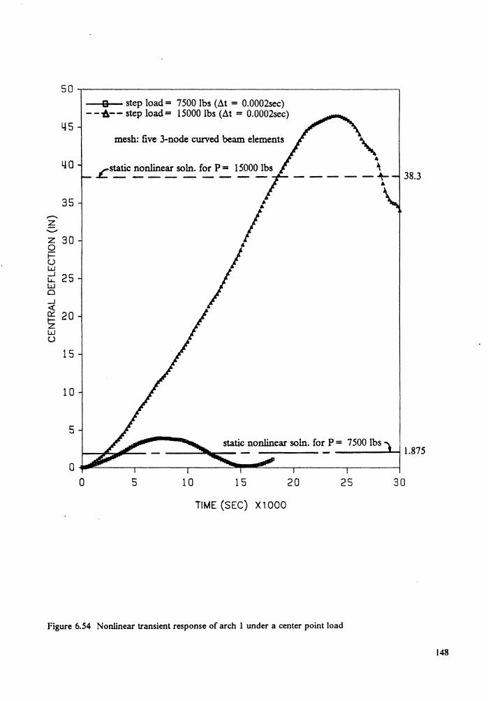
50 B step load= 7500 lbs (~t = 0.0002sec)
- --A-- step load= 15000 lbs (~t = 0.0002sec) 45
mesh: five 3-node curved beam elements ' L!O 4
.£static nonlinear soln. for P = 15000 lbs \ - --------r-----t- 38.3
35 • • ,,...... I z '-"' z 30 0 ' F
I (.) w _J 25 Li... w 0 _J <( a:: 20 I I-z w u
15
10
5
o---~~-.~~~.--~~~111111!!':~--.-~~~....-~~~
0 s 10 15 20 25 30
TIME (SEC) X 1000
Figure 6.54 Nonlinear transient response of arch 1 under a center point load
148
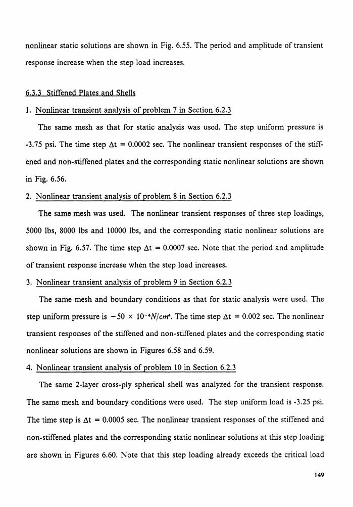
nonlinear static solutions are shown in Fig. 6.55. The period and amplitude of transient
response increase when the step load increases.
6.3.3 Stiffened Plates and Shells
I. Nonlinear transient analysis of problem 7 in Section 6.2.3
The same mesh as that for static analysis was used. The step uniform pressure is
-3.75 psi. The time step At = 0.0002 sec. The nonlinear transient responses of the stiff-
ened and non-stiffened plates and the corresponding static nonlinear solutions are shown
in Fig. 6.56.
2. Nonlinear transient analysis of problem 8 in Section 6.2.3
The same mesh was used. The nonlinear transient responses of three step loadings,
5000 lbs, 8000 lbs and 10000 lbs, and the corresponding static nonlinear solutions are
shown in Fig. 6.57. The time step At = 0.0007 sec. Note that the period and amplitude
of transient response increase when the step load increases.
3. Nonlinear transient analysis of problem 9 in Section 6.2.3
The same mesh and boundary conditions as that for static analysis were used. The
step uniform pressure is -50 x 10- 4N/cnf. The time step At = 0.002 sec. The nonlinear
transient responses of the stiffened and non-stiffened plates and the corresponding static
nonlinear solutions are shown in Figures 6.58 and 6.59.
4. Nonlinear transient analysis of problem 10 in Section 6.2.3
The same 2-layer cross-ply spherical shell was analyzed for the transient response.
The same mesh and boundary conditions were used. The step uniform load is -3.25 psi.
The time step is At = 0.0005 sec. The nonlinear transient responses of the stiffened and
non-stiffened plates and the corresponding static nonlinear solutions at this step loading
are shown in Figures 6.60. Note that this step loading already exceeds the critical load
149
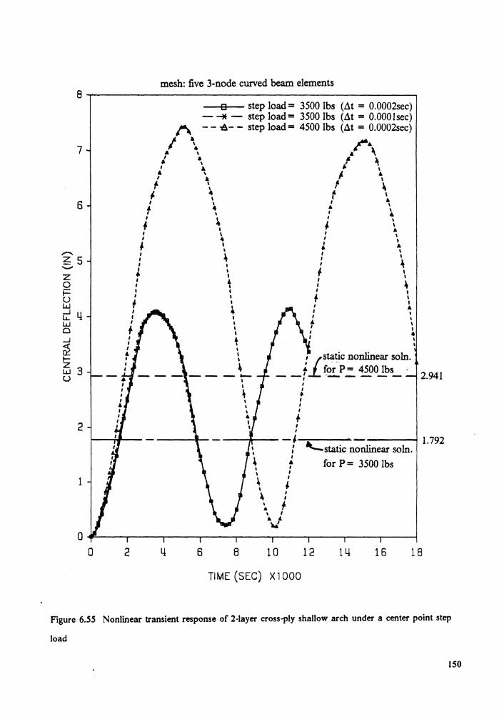
7
6
,-... 6; 5 -z 0 g ~ 4 w 0 ...J
Ci ~ w 3 u
2
1
0
I I I • I
2
mesh: five 3-node curved beam elements
a step load= 3500 lbs (.1t = 0.0002sec) - ~ - step load= 3500 lbs (.1t = O.OOOlsec)
I'\ - - -6- - step load= 4500 lbs (.1t = 0.0002sec)
I \ /"• ! \ & ' i , I ~
I & /. ~ ,. \ ,. ~
/. 4 " \ I I I • \ I \ t •, • ' I 4
# \ j \ \ I • I
I
# I I I
l I I I I
+
6
4 I \ I I I ' .. . \ I \ : ~ I
' I + 1 I I I I ..
I I I
f
I I
~ t I I • I I
' I • I I 'i static nonlinear soln. - -f ~~p~ 4500 lbs_. 2.941
I I ..
I I I
+ I I
----_, ____ ___. 1.792 : '-static nonlinear soln. I , t for P= 3500 lbs
\ '
8
~ I
' ' ~ : ~ I
\ I
\./
10
TIME (SEC) X 1000
12 14 16 18
Figure 6.SS Nonlinear transient response of 2-layer cross-ply shallow arch under a center point step
load
150
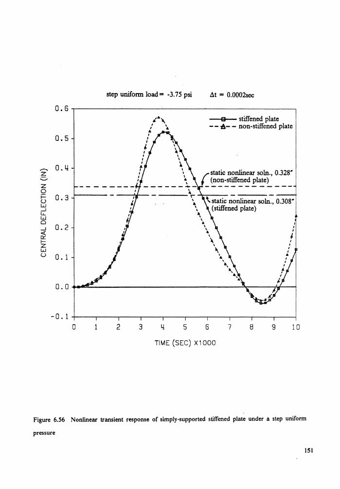
0.5
'"'""' 0. I.! z .......... z 0 I- 0.3 u w _J u.._ w 0 _J 0.2 <( ll:'. I-z w u a. 1
0 1
step uniform load= -3.75 psi At = 0.0002sec
2 3
\ 4
\
' \ 4
\ --------'
a stiffened plate - - ~- - non-stiffened plate
( static nonlinear soln., 0.328"' (non-stiffened plate) -------------
----'\- ~....,---- - - __ _. \static nonlinear soln., 0.308"'
(stiffened plate)
4 5
\ ... \ \ ...
\ \ ..
\ \
" \ \
6
TIME (SEC) X 1000
7 8 9
I I ,
~
10
Figure 6.56 Nonlinear transient response of simply-supported stiffened plate under a step uniform
pressure
151
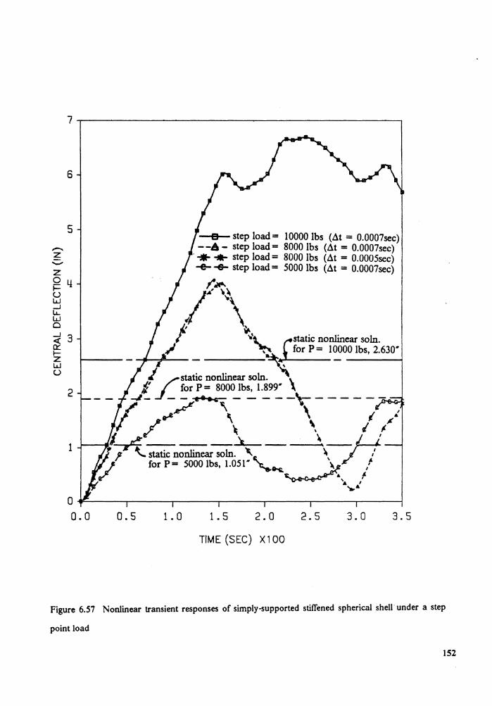
,-... z
......... z 0 I-u w _J \.l... w 0 _J
< 0:: I-z w u
6
5 B step load= 10000 lbs (At = 0.0007sec)
--A - step load= 8000 lbs (At = 0.0007sec) -+ + step load= 8000 lbs (At = 0.0005sec) ~ ~ step load= 5000 lbs (At = 0.0007sec)
14
3
2
~~
/"'~ I~ \,
~\._ 14static nonlinear soln. -....-;:. ..... ~- _____ ._~'.-'\•~for P = 10000 lbs, 2.630"
/ /static nonlinear soln. ' -.I~ J _ for ;.=.::O~b:_ I.899" \\-:- _____ _
{ .,,.F \ \ '~' 1
'l / \ \ 'l 1----41'~ - --'-- - --j-j ! \. static nonlinear soln. ~ ~ ,' ~ for P= 5000 lbs, 1.051" '-..~~, f/
.I. I ....... o~~~--.-~~-,-~~--.~~~.--~~~~~~~~-J
o.o o.s 1. 0 1. 5 2.0 2.5 3.0 3.5
TIME (SEC) X 100
Figure 6.57 Nonlinear transient responses of simply-supported stiffened spherical shell under a step
point load
152
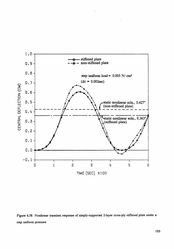
1. 0
0.9
0.8
,--..., 0.7 ~ (.) ..__,,,
0.6 z 0 ~ 0.5 (.) w .....J LL w 0.4 0 .....J <{ CY 0.3 t-z w (.) 0.2
0. 1
0.0
-0. 1 0 1
a stiffened plate - -Ir - non-stiffened plate
2
step uniform load= 0.005 N/ cm2
(~t = 0.002sec)
3 5
TIME (SEC) X 100
6
Figure 6.58 Nonlinear transient response of simply-supported 2-layer cross-ply stiffened plate under a
step uniform pressure
153
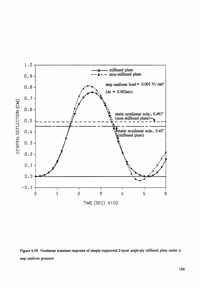
1. 0
0.9
0.8
,....... 0.7 ~ u .._.,
0.6 z 0 i=
0.5 u w __J lJ._ w 0.4 0 _J <( D::'. 0.3 f-z w u 0.2
0. 1
0.0
-0. 1 0 1 2
a stiffened plate - - 6 - - non-stiffened plate
3
step uniform load= 0.005 N / cm2
(i1t = 0.002sec)
static nonlinear solo., 0.491" \ (non-stiffened plate)~ _________ 1 __
\ static nonlinear solo., 0.45" \(stiffened plate)
4 5
TIME (SEC) X 1 00
6
Figure 6.59 Nonlinear transient response of simply-supported 2-layer angle-ply stiffened plate under a
step uniform pressure
154
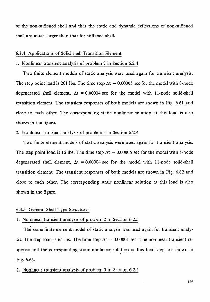
of the non-stiffened shell and that the static and dynamic deflections of non-stiffened
shell are much larger than that for stiffened shell.
6.3.4 Applications of Solid-shell Transition Element
1. Nonlinear transient analysis of problem 2 in Section 6.2.4
Two finite element models of static analysis were used again for transient analysis.
The step point load is 201 lbs. The time step Lit = 0.00005 sec for the model with 8-node
degenerated shell element, Lit = 0.00004 sec for the model with 11-node solid-shell
transition element. The transient responses of both models are shown in Fig. 6.61 and
close to each other. The corresponding static nonlinear solution at this load is also
shown in the figure.
2. Nonlinear transient analysis of problem 3 in Section 6.2.4
Two finite element models of static analysis were used again for transient analysis.
The step point load is 15 lbs. The time step Lit = 0.00005 sec for the model with 8-node
degenerated shell element, Lit = 0.00004 sec for the model with 11-node solid-shell
transition element. The transient responses of both models are shown in Fig. 6.62 and
close to each other. The corresponding static nonlinear solution at this load is also
shown in the figure.
6.3.5 General Shell-Type Structures
1. Nonlinear transient analysis of problem 2 in Section 6.2.5
The same finite element model of static analysis was used again for transient analy-
sis. The step load is 65 lbs. The time step Lit = 0.00001 sec. The nonlinear transient re-
sponse and the corresponding static nonlinear solution at this load step are shown in
Fig. 6.63.
2. Nonlinear transient analysis of problem 3 in Section 6.2.5
155
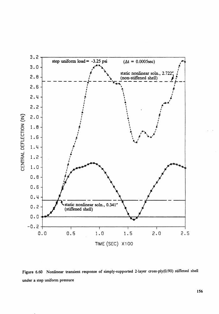
3.2
3.0
2.8
2.6
2.4
2.2 ,.....,.
2.0 z ....... z 1. 8 0 i= u 1. 6 w _J Li.. w 1. 4 0 _J <1.'. 1. 2 0:: ~ w 1. 0 u
0.8
0.6
0.4
0.2
o.o -0.2
0.0
step uniform load= -3.25 psi (.6.t = O.OOOSsec) ~ ~~ 1 A .. I
' .... I /. \ static nonlinear soln., 2. 722j :
/ \ (non-stiffened shell) ' f -------~----r.-----------~-, ~ ,
I \ I I & ~ I \ I I \ I
t \ J I \ I I A ...... I I 4 I \ I I I I
& I I
: \ I I A I I I I t I I
f \ ' I I I
: ~ ,•'4 ,' I. \ I- 'A•' I \ I
,' •., "' I
I I ,.
I I I
f
static nonlinear soln., 0.341"' (stiffened shell)
0.5 1. 0 1. 5
TIME (SEC) X100
2.0 2.5
Figure 6.60 Nonlinear transient response of simply-supported 2-layer cross-ply(0/90) stiffened shell
under a step uniform pressure
156
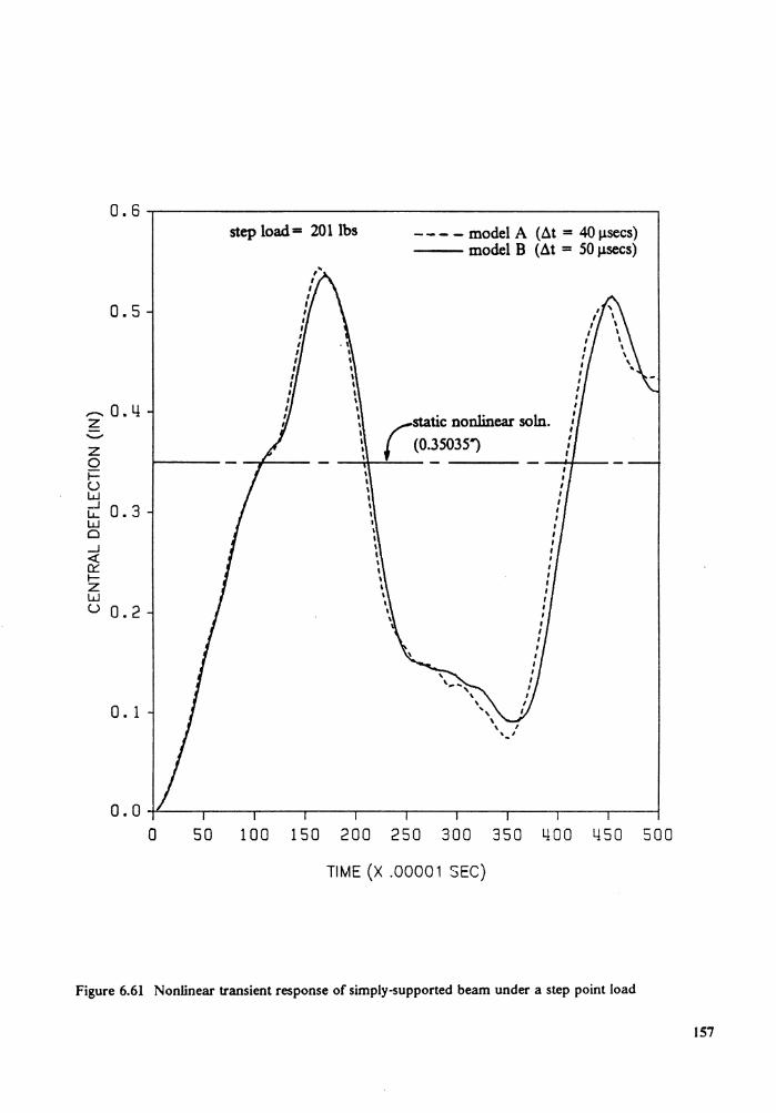
0.5
,_ 0. 4 z ......... z 0 I-u w _J 0.3 LL w 0 _J ~ 0::: I-z w u 0.2
0. 1
0 50
step load= 201 lbs - - - - model A (~t = 40 µsecs) -- model B (~t = 50 µsecs)
(0.35035}
I I
I I
I I I I I I I I I I I I I I I
(static nonlinear soln.
~~--'~-- ~+'----
100 150 200 250 300 350 400 450 500
TIME (X .00001 SEC)
Figure 6.61 Nonlinear transient response of simply-supported beam under a step point load
157
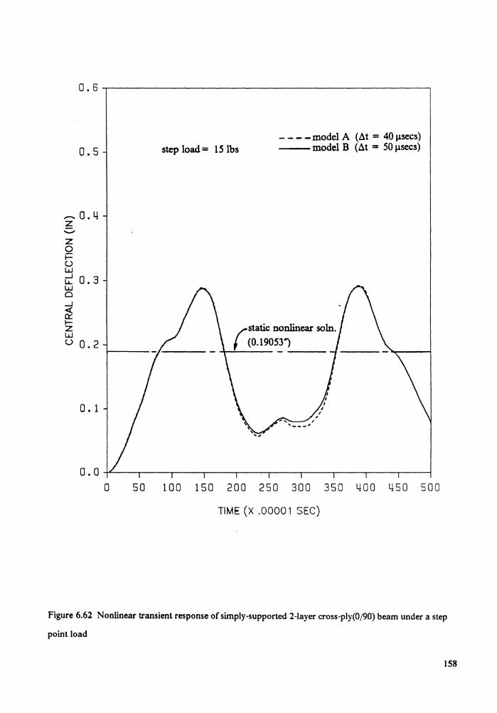
0.5
,...... a. 4 z -z 0 t> w ~ a. 3 w Cl _J <( a::: ~ w (.) 0.2
0. 1
- - - -model A (&t = 40 µsecs) step load= 1 S lbs --model B (&t = SO µsecs)
0 50 100 150 200 250 300 350 400 450 500
TIME (X .00001 SEC)
Figure 6.62 Nonlinear transient response of simply-supported 2-layer cross-ply(0/90) beam under a step
point load
158
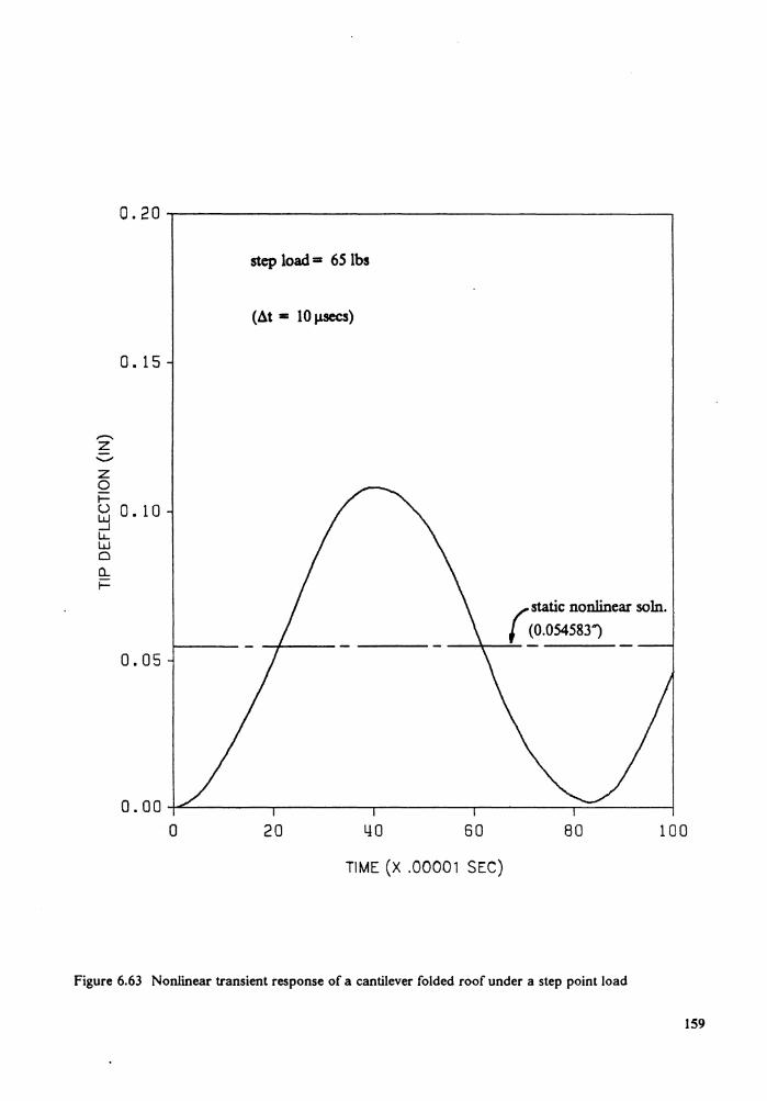
z 0 1-
0. 15
(.) 0.10 ~ lJ... w 0 CL F
0.05
step load == 65 lbs
(At = 10 µsecs)
(static nonlinear soln. (0.054583}
-~--- -
0.00+-"'-------.-------,..-----...--------.--"-------l 0 20 40 60 80 100
TIME (X .00001 SEC)
Figure 6.63 Nonlinear transient response of a cantilever folded roof under a step point load
159

The same finite element models of static analysis were used again for transient anal-
ysis. The step load is 63 lbs. The time step ~t = 0.00008 sec. The nonlinear transient
responses of these two finite element models and the corresponding static nonlinear
solutions at this load step are shown in Fig. 6.64.
3. Nonlinear transient analysis of problem 4 in Section 6.2.5
The same finite element model as that of static analysis was used again for transient
analysis. The step load is 18 lbs. Fig. 6.65 shows the nonlinear transient responses for
two different time step, 0.00005 sec and 0.0001 sec, which are close to each other. The
static nonlinear deflection at this load step is also shown in the figure.
160
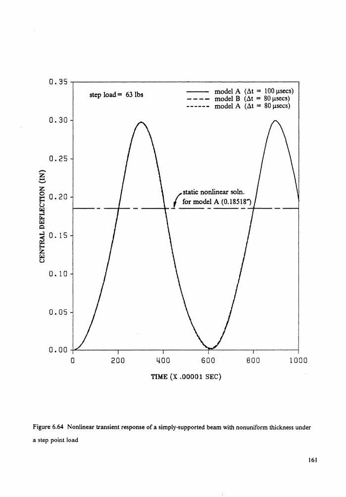
-z -"-' z 0 e::: t,.) ~ ..J r:i;. ~ Q ...:l
ca E--< z ~ t,.)
step load= 63 lbs
0.30
0.25
0.20
0. 15
0. 10
0.05
model A (At = 100 µsecs) ---- model B (At= 80µsecs) ------ model A (At = 80 µsecs)
static nonlinear soln. /for mod~ A (0.185~}
0.00..+L.~~~--..~~~~-.-~~~~~~~~-,-~~~---t
0 200 400 600 800 1000
TIME (X .00001 SEC)
Figure 6.64 Nonlinear transient response of a simply-supported beam with nonuniform thickness under
a step point load
161
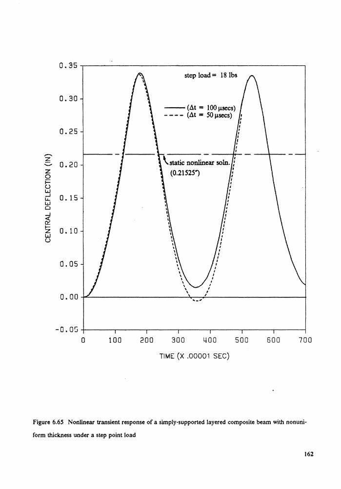
0.35 step load= 18 lbs
0.30 (.1t = 100 µsecs) (.1t = 50 µsecs)
0.25
,-....
\.static nonlin~ soln. f z .._,, 0.20 z (0.21525}
I I
0 I
t> I I I
w _J 0. 15 LL. w I
I 0 I I
.....J I I I I
<! \ I ():'.: I I
I- I I z 0. 10 I I
I I w I I (.) I I
I I \ I \ I \ I \ I
0.05 \ I I I
I I
I I
I I
I o.oo , .. _ ..
0 100 200 300 l.!00 500 600 700
TIME (X .00001 SEC)
Figure 6.65 Nonlinear transient response of a simply-supported layered composite beam with nonuni-
form thickness under a step point load
162
CHAPTER 7
CONCLUSIONS AND RECOMMENDATIONS
7.1 Summary and Conclusions
The present study dealt with the following major topics:
1. The formulation of incremental equations of motion of a continuum by the total
Lagrangian description based on the principle of virtual displacements.
2. The development of displacement finite element model from the linearized incre-
mental equations of motion by the continuum mechanics strain-displacement re-
lations and interpolations of coordinates and displacements.
3. Time discretization of the equations of motion and construction of solution proce-
dures to solve the system equations iteratively for nonlinear analysis.
4. Imposing some assumptions from shell and beam theories on the 3-dimensional
isoparametric continuum element to develope continuum-based shell, beam and
solid-shell transition elements for anisotropic as well as isotropic materials.
Numerical examples, for both static and transient analyses, demonstrate the validity
and efficiency of the present formulations and solution procedures. The present results
are in good agreement with those available in the literature. Many of the numerical re-
sults of general shell-type structures included here can serve as references for future in-
vestigations. The present work is the one which can analyze isotropic and laminated
general shell-type structures accurately and efficiently.
163
7.2 Recommendations
The formulations presented here can be extended to contain more considerations in
practical structural analysis. The inclusion of thermal load in the present formulations
is straight forward since the temperature field within the element can be interpolated in
the similar way as displacement field. Also if the membrane strains are large, the thick-
ness is updated by evaluating the normal strain increments from the constitutive
equations via the zero normal stress assumption.
The present formulations can be extended to incorporate with nonlinear material
models, for example plasticity and nonlinear viscoelasticity, in case the improved
anisotropic material models are available. The materially nonlinear analysis can be per-
formed either seperately or in combination with geometric nonlinearity.
Another natural extension of the present research is to incorporate with failure cri-
teria to deal with the failure analysis of laminated composite structures.
One area which needs more study is the cost reduction and accuracy of nonlinear
analysis for complex practical structures, e.g. the structures with cut-out or discontin-
uous stiffeners which need more detailed stress analysis near the discontinuities. The
development of global/local algorithms may greatly improve efficiency. The combina-
tion of present formulations with some global/local analysis strategies is therefore worth
future investigation.
164
REFERENCES
1. 0. C. Zienkiewicz, The Finite Element Method, McGraw-Hill, N. Y., 1976.
2. J. N. Reddy, An Introduction to the Finite Element Method, McGraw-Hill, N. Y., 1984.
3. R. H. Gallagher, "Shell elements", in Proc. of World Congress on Finite Elements in Struct. Mech., Vol. l, Bournemouth, England, 1975.
4. T. H. H. Pian and P. Boland, "Formulation of large deflection shell analysis by as-sumed stress finite element method", in Formulations and Computational Algo-rithms in Finite Element Analysis, K. J. Bathe, J. T. Oden and W. Wunderlich (eds.), M. I. T. Press, Mass., 1977.
5. A. K. Noor and S. J. Hartly, "Nonlinear shell analysis via mixed isoparametric ele-ments", Computers and Structures, Vol. 7, pp. 615-626, 1977.
6. B. M. Irons, "Engineering application of numerical integration in stiffness methods", AIAA J., Vol. 4, pp. 2035-2037, 1966.
7. J. Ergatoudis, B. M. Irons and 0. C. Zienkiewicz, "Three-dimensional stress analysis of arch dams by the finite element method", Reseach Report No. C.P. 58/66, Univ. of Wales, Swansea.
8. J. Ergatoudis, B. M. Irons and 0. C. Zienkiewicz, "Curved isoparametric quadrilateral element", Int. J. Solids Structures, Vol. 4, pp. 31-42, 1968.
9. J. Ergatoudis, B. M. Irons and 0. C. Zienkiewicz, "Three-dimensional stress analysis of arch dams and their foundations", Proc. Symp. Arch Dams, Inst. Civ. Engrs, London; pp. 37-50, 1968.
10. J. N. Reddy and T. Kuppusamy, "Analysis of layered composite by three-dimensionsl elasticity theory", Research Report No. VPI-E-82.31, VPI and State Univ., Blacksburg, Va., 1980.
11. S. Ahmad, B. M. Irons and 0. C. Zienkiewicz, "Analysis of thick and thin shell structures by curved finite elements", Int. J. Numer. Meth. Eng., Vol. 2, pp. 419-451, 1970.
165
. /
12. E. Ranlm., "A Plate/shell element for large deflections and rotations", in Formu-lations and Computational Algorithms in Finite Element Analysis, K. J. Bathe, J. T. Oden and W. Wunderlich (eds.), M. I. T. Press, 1977.
13. B. Krakeland, "Large displacement analysis of shells considering elastic-plastic and elasto-viscoplastic materials", Report No. 776, The Norwegian Inst. of Tech., Norway, 1977.
14. T. Y. Chang and K. Sawamiphakdi, "Large deformation analysis of laminated shells by finite element method", Computers Struct., Vol. 13, pp. 331-340, 1981.
15. K. J. Bathe, Finite Element Procedures in Engineering Analysis, Prentice-Hall, N. J., 1982.
16. K. J. Bathe and S. Bolourchi, "A geometric and material nonlinear plate and shell element", Computers Struct., Vol. 11, pp. 23-48, 1980.
17. W. C. Chao and J. N. Reddy, "Analysis of laminated composite shells using a de-generated 3-D element", Int. J. Numer. Meth. Eng., Vol. 20, pp. 1991-2007, 1984.
18. P. C. Kohnke and W. C. Schnobrich, "Analysis of eccentrically stiffened cylindrical / shells", J. of Structural Div., ASCE, Vol. 98, pp. 1493-1510, 1972.
19. A. Venkatesh and K. P. Rao, "A laminated anisotropic Curved beam and shell stiffening finite element", Computers Struct., Vol. 15, pp. 197-201, 1982 .
20. K. P. Rao, "A rectangular laminated anisotropic shallow thin shell finite element", Comput. Meths. Appl. Mech. Engrg., Vol. 15, pp. 13-33, 1978.
21. A. Venkatesh and K. P. Rao, "Analysis of laminated shells with laminated stiffeners using rectangular finite elements", Comput. Meths. Appl. Mech. Engrg., Vol. 38, pp. 255-272, 1983.
22. A. Venkatesh and K. P. Rao, "Analysis of laminated shells of revolution with lami-nated stiffeners using a doubly curved quadrilateral finite element", Computers Struct., Vol. 20, pp. 669-682, 1985.
23. A. Venkatesh and K. P. Rao, "A doubly curved quadrilateral finite element for the analysis of laminated anisotropic thin shells of revolution", Computers Struct., Vol. 12, pp. 825-832, 1980.
166
24. A. J. Carr and R. W. Clough, "Dynamic earthquake behavior of shell roofs", Fourth World Conf. on Earthquake Engineering, Santiago, Chile, 1969.
25. L. A. Schmit, "Developments in discrete element finite deflection structural analysis by function minimization", Technical Report AFFDL-TR-68-126, Wright-Patterson Air Force Base, Ohio, 1968.
26. G. H. Ferguson and R. H. Clark, "A variable thickness curved beam and shell stiff-ening element with shear deformations", Int. J. Numer. Meth. Eng., Vol. 14, pp. 581-592, 1979.
27. G. Horrigmoe and P. G. Bergan, "Incremental variational priniciple and finite ele-ment models for nonlinear problems", Computer Meth. Appl. Mech. Engrg., Vol. 7, pp. 201-217, 1976.
28. W. Wunderlich, "Incremental formulations for geometrically nonlinear problems", in Formulations and Algorithm in Finite Element Analysis, K. J. Bathe, J. T. Oden and W. Wunderlich (eds.), pp. 193-239, M. I. T. Press, 1977.
29. J. A. Stricklin, W. A. Von Riesemann, J. R. Tillerson and W. E. Haisler, "Static geometrical and material nonlinear analysis", Adv. in Comp. Meth. in Struct. Mech. and Design, J. T. Oden, R. W. Clough and Y. Yamamoto (eds.), Univ. of Alabama in Huntsville, pp. 301-324, 1972.
30. K. J. Bathe, E. Ramm and E. L. Wilson, "Finite element formulations for large de-formation dynamic analysis", Int. J. Numer. Meth. Engrg., Vol. 9, pp.353-386, 1975.
31. S. Yaghmai and E. P. Popov, "Incremental analysis of large deflections of shells of revolution", Int. J. Solids Struct., Vol.7, pp. 1375-1393, 1971.
32. Y. Yamada, "Incremental formulations for problems with geometric and material nonlinearities", Adv. in Comp. Meth. in Struct. Meth. and Design, J. T. Oden, R. W. Clough and Y. Yamamoto (eds.), Univ. of Alabama in Huntsville, pp. 325-355, 1972.
33. W. Kanok-Nukulchai, R. L. Taylor and T. J. R. Hughes," A large deformation for-mulation for shell analysis by the finite element method", Computers Struct., Vol. 13, pp. 19-27, 1981.
34. P. Sharifi and E. P. Popov, "Nonlinear buckling analysis of sandwich arches", J. Engrg. Mech. Div., ASCE, Vol. 97, pp. 1397-1411, 1981.
167
35. A. C. ·walker, "A nonlinear finite element analysis of shallow circular arches", Int. J. Solids Struct., Vol. 5, pp. 97-107, 1969.
36. A. K. Noor, W.H. Greene and S. J. Hartley, "Nonlinear finite element analysis of curved beams", Comp. Meth. Appl. Mech. Engrg., Vol. 12, pp. 289-307, 1977.
37. A. K. Noor and J. M. Peters, "Mixed models and reduced/selective integration dis-placement models for nonlinear analysis of curved beams", Int. J. Numer. Meth. Engrg., Vol. 17, pp. 615-631, 1981.
38. L. E. Malvern, Introduction to The Mechanics of A Continuous Medium, Prentice-Hall, N. J., 1974. &)Ag-I'>'°',.~ , .. f3>
39. P. G. Bergan, G. Horrigmoe, B. Krakeland and T. H. Soreide, "Solution techniques for nonlinear finite element problems", Int. J. Numer. Meth. Engrg., Vol. 12, pp. 1677-1696, 1978.
40. P. G. Bergan and T. H. Soreide, "Solution of large displacement and instability problems using the current stiffness parameter", Finite Elements in Nonlinear Me-chanics, pp. 647-649 Tapir Press, 1978.
41. J. H. Argyris, "Continua and discontinuaH, Proc. 1st Conf. Matrix Meth. Struct. Mech., Wright-Patterson A.F.B., Ohio, pp. 11-189, 1965.
' 42. J. L. Batoz and G. Dhatt, "Incremental displacement algorithms for nonlinear problems", Int. J. Numer. Meth. Engrg., Vol. 14, pp. 1262-1266, 1979.
43. E. Riks, "An incremental approach to the solution of snapping and buckling prob-lem", Int. J. Solids Structures, Vol. 15, pp. 529-551, 1979.
44. E. Ramm, "Strategies for tracing the nonlinear response near limit points", Nonlin-ear Finite Element Analysis in Structural Mechanics (Eds. Wunderlich, Stein, Bathe), pp. 63-89, Spring-Verlag, 1981.
45. M. A. Crisfield, "A fast incremental/iterative solution procedure that handles snap-through", Computers Struct., Vol. 13, pp. 55-62, 1981.
46. G. A. Wempner, "Discret approximations related to nonlinear theories of solids", Int. J. Solids Structures, Vol. 7, pp. 1581-1599, 1971.
168
47. S. M. Holzer, L. T. Watson and P. Vu., "Stability analysis of lamella domes", Proc. of the ASCE Symposium on Long Span Roof Structures, St. Louis, Mo., pp. 179-209, 1981.
48. K. J. Bathe and E. N. Dvorkin, "On the automatic solution of nonlinear finite ele-ment equations", Computers Struct. Vol. 17, pp. 871-879, 1983.
49. K. J. Bathe and L. W. Ho, "Some resulte in the analysis of thin shell structures", Nonlinear Finite Element Analysis in Structural Mechanics (Eds. Wunderlich, Stein, Bathe), pp. 122-150, Spring-Verlag, 1981.
50. K. S. Surana, "Transition finite elements for three-dimensional stress analysis", Int. J. Numer. Meth. Engrg., Vol. 15, pp. 991-1020, 1980.
51. K. S. Surana, "Geometrically nonlinear formulation for the three dimensional solid-shell transition finite elements", Computers Struct., Vol. 15, pp. 549-566, 1982.
52. C. Truesdell and W. Noll, The Nonlinear Field Theories of Mechanics; Encyclopedia of Physics (Ed. S. Flugge ), II 1/3, Springer-Verlag, 1965.
53. K. J. Bathe and A. P. Cimento, "Some practical procedures for the solution of non-linear finite element equations", J. Computer Methods in Applied Mechanics and Engineering, Vol. 22, pp. 59-85, 1980.
54. S. C. Panda and R. Natarajan, "Finite element analysis of laminated composite plates", Int. J. Numer. Meth. Engrg., Vol. 14, pp. 69-79, 1979.
55. 0. C. Zienkiewicz, R. L. Taylor and J. M. Too, "Reduced Integration Techniques in general analysis of plates and shells", Int. J. Numer. Meth. Engrg., Vol. 3, pp. 275-290, 1971.
56. A. C. Scordelis and K. S. Lo, "Computer analysis of cylindrical shells", ACI J oumal, Vol. 61, pp. 539-561, 1964
57 .. K. J. Bathe and L. W. Ho, "A simple and effective element for analysis of general 'shell structures", Computers Struct. Vol. 13, pp. 673-681, 1981.
58. J. N. Reddy, "A note on symmetry considerations in the transient responae of un-symmetrically laminated anisotropic plates", Int. J. Numer. Meth. Engrg., Vol. 20, pp. 175-181, 1984.
169
59. J. N. Reddy, "On the solutions to forced motions of rectangular composite plates", J. Appl. Mech., Vol. 49, pp. 403-408, 1982.
60. S. A. Zaghloul and J. B. Kennedy, "Nonlinear Behavior of Symmetrically laminated plates", J. Appl. Mech., Vol. 42, pp. 234-236, 1975.
61. N. S. Putcha and J. N. Reddy, "A refined mixed shear flexible finite element for the nonlinear analysis of laminated plates", Computers Struct., Vol. 22, pp. 529-538, 1986.
62. K. Chandrashekhara, "Geometric and Material nonlinear analysis of laminated composite plates and shells", Ph.D. Thesis, ESM Dept., VPI and State University, Blacksburg, Va., 1985.
63. S. Timoshenko, Strength of Materials, Part II, 2nd ed., Van Nostrand, Amsterdam, 1947.
64. J. N. Reddy and P.R. Heyliger, "A mixed updated Lagrangian formulation for plane elastic problems", Research Report, VPI and State University, Blacksburg, Va., 1986.
65. G. M. Stanley and C. A. Felippa, "Computational procedures for postbuckling of composite shells", Finite Element Methods for Nonlinear Problems (Eds. Bergan, Bathe, Wunderlich), pp. 359-385, Springer-Verlag, 1986.
66. S. Timoshenko and S. W. Krieger, Theory of Plates and Shells, McGraw-Hill, N.Y., 2nd ed., 1959.
67. J. N. Reddy, Energy and Variational Methods in Applied Mechanics, John Wiley, N.Y., 1984.
68. J. N. Reddy, "Geometrically nonlinear transient analysis of laminated composite plates", AIAA Journal, Vol. 21, pp. 621-629, 1983.
69. D. P. Mondkar and G. H. Powell, "Finite element analysis of nonlinear static and dynamic response", Int. J. Numer. Meth. Engrg, Vol. 11, pp. 499-520, 1977.
70. H. Schreyer and E. Masur, "Buckling of Shallow Arches", J. of the Engrg. Mech. Div., ASCE, Vol. 92, No. EM4, pp. 1-19, 1966.
170
APPENDIX
A.1 A clamped hypar shell
The geometry and boundary conditions of a clamped hypar shell are shown in Fig.
A. I. Full shell was modelled with sixteen 9-node shell elements because no symmetric
bending exists for this problem. The clamped shell is subjected to a uniform lateral
pressure P., = -0.01 psi. The linear deflection at the center obtained in the present study
is -0.024442 in as compared with -0.024082 in obtained by Rao [20] who used sixteen
4-node shell elements based on a classical thin shell theory.
A.2 Stress variations of problem 10 in Section 6.2.3
The stress variations of 2-layer cross-ply simply-supported stiffened spherical shell
with respect to the loading are plotted in Figures A.2 and A.3. The stresses were meas-
ured at the apex of the stiffened shell for each load step. Fig. A.2 shows the stresses
within the shell while Fig. A.3 shows the stresses within the stiffeners.
171
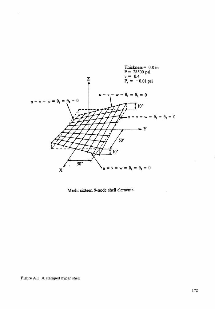
z
Thickness= 0.8 in E= 28500 psi v = 0.4 P. = -0.01 psi
Mesh: sixteen 9-node shell elements
Figure A.l A clamped hypar shell
172
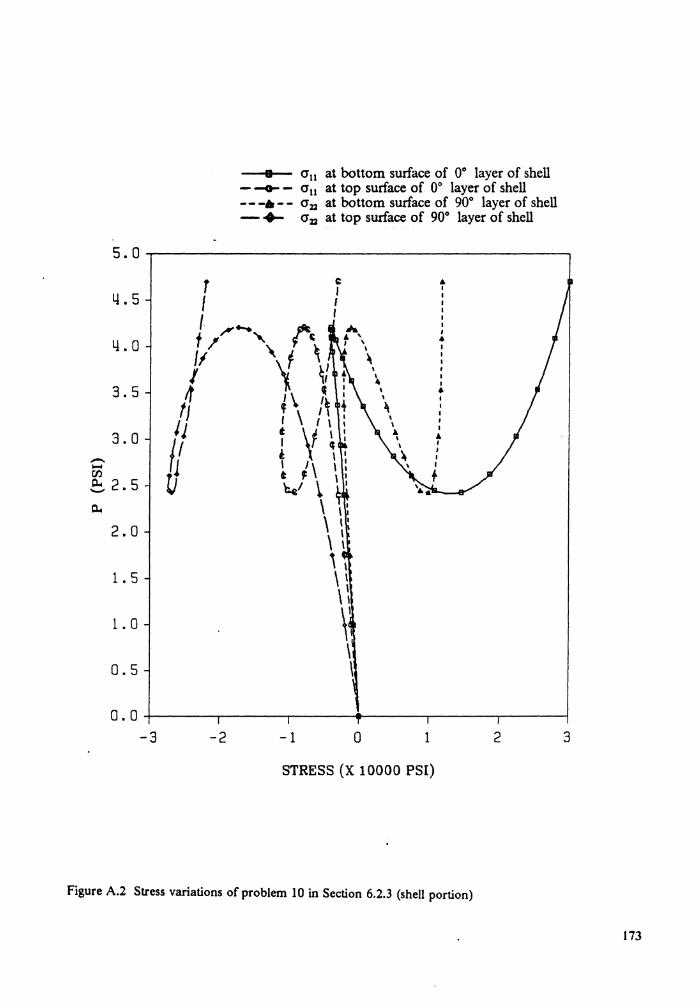
-..... Cll
L!. 5
L!. 0
3.5
3.0
~ 2. 5 c..
2.0
1. 5
1. 0
0.5
T I
a a 11 at bottom surface of 0° layer of shell - -o- - a 11 at top surface of 0° layer of shell -- -•- - cr:D at bottom surface of 90° layer of shell - +- cr:D at top surface of 90° layer of shell
I .... 1't. t I'/ " ~ ~
}1 ... \t \: t tt l. • I
t 4 \\ I~ + J j I I \ :
II I V ~: I I I\ \ : rt t ' 1•
\j 'c.e/ ~ ~I \ , . \ , . \ \ ' \ \ \ \ \ \' \ \
0.0-1-~~~.--~~~~~~-+~~~-r-~~~,.....-~~---j
-3 -2 -1 0 1 2 3
STRESS (X 10000 PSI)
Figure A.2 Stress variations of problem 10 in Section 6.2.3 (shell portion)
173
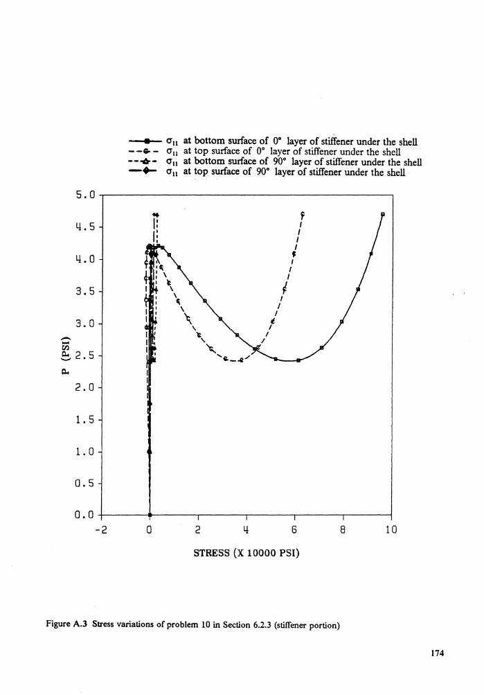
4.5
LL 0
3.5
3.0 --en ~ 2. 5 Q.,
2.0
1. 5
1. o
0.5
• a 11 at bottom surface of 0° layer of stiffener under the shell - -• - a 11 at top surface of 0° layer of stiffener under the shell --•· a 11 at bottom surface of 90° layer of stiffener under the shell -~ a 11 at top surface of 90° layer of stiffener under the shell
... 1: ll
I
f , I I I
' I I I
I I
I I
' I I
0.0-1-~~-*~~~.-~~--.-~~----,,-~~,-~~-1
-2 o 2 6 8 10
STRESS (X 10000 PSl)
Figure A.3 Stress variations of problem 10 in Section 6.2.3 (stiffener portion)
174

The vita has been removed from the scanned document


![FINITE ELEMENT ANALYSIS OF SHELL STRUCTURES · hemispherical shell considering the introduction of large displacements ... and Shells” by J.N. Reddy [5] is recommended. 3. The Finite](https://img.pdfslide.us/doc/110x75/5b87f3657f8b9a46538cbf6a/finite-element-analysis-of-shell-structures-hemispherical-shell-considering.jpg)