Embed Size (px)
Citation preview
CONTINUUM SHELL ELEMENT AND POSTBUCKLING ANALYSIS
Description of continuum shell element(principle of virtual displacements)
Post-buckling analysis of composite panels and comparison with experimental results
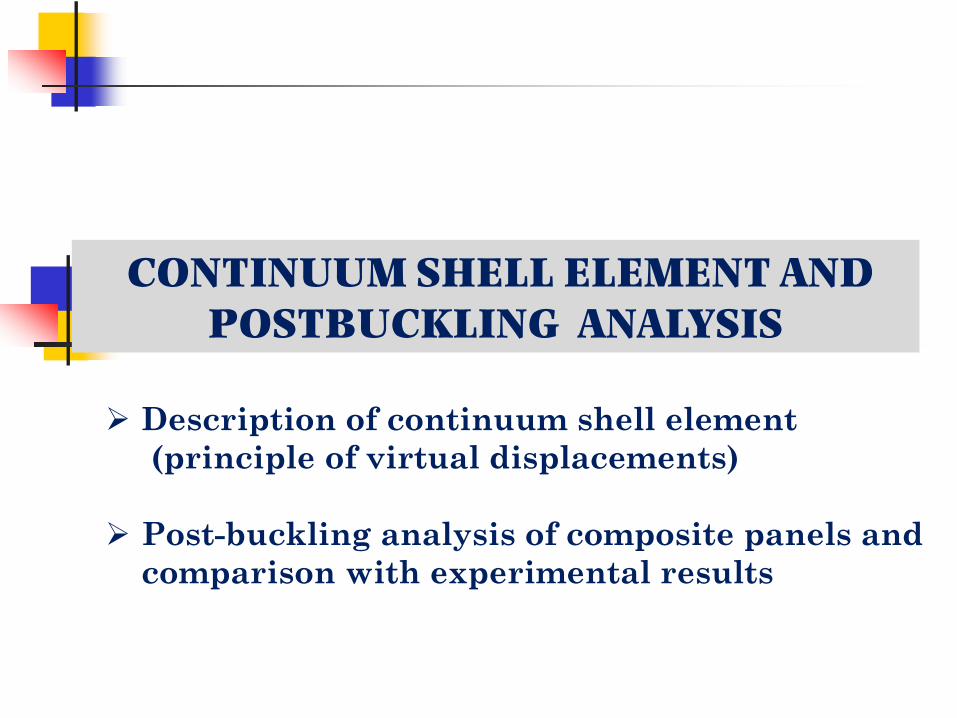
CONTINUUM SHELL ELEMENT
J N Reddy
1 1,X x
2 2,X x
3 3,X x
e3ˆ e1ˆE1ˆE3
ˆ
e2ˆE2ˆ
00Ω Ω
1Ω
10S
0d V
12Ω 2
rΩ2Ω1
2rΩ
0d S
10E
0
Equilibrium iterations
0S
20S20E
Continuum Shell Element 2
CONTINUUM SHELL ELEMENT
Z
0V
t+¢t0 Sij ±(t+¢t
0 "ij)0dV = t+¢tR
t+¢tR =
Z
0A
t+¢t0 tk ±uk
0dA +
Z
0V
0½ t+¢t0 fk ±uk
0dV
Z
t+¢tV
t+¢t¾ij ±t+¢teijt+¢tdV = t+¢tR
Z
t+¢tV
t+¢ttij ±(t+¢teij)t+¢tdV =
Z
0V
t+¢t0 Sij ±(t+¢t
0 "ij)0dV
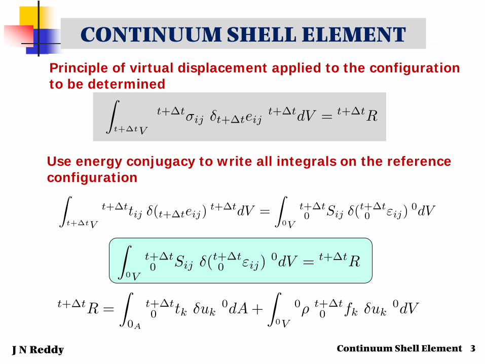
Principle of virtual displacement applied to the configuration to be determined
Use energy conjugacy to write all integrals on the reference configuration
Continuum Shell Element 3J N Reddy
CONTINUUM SHELL ELEMENT
±(t+¢t0 "ij) = ±(t
0"ij) + ±(0"ij) = ±(0"ij)
0Sij = 0Cijrs 0"rs; 0Sij = 0Cijrs 0`rs
Z
0V0Cijrs 0`rs ±(0"ij)
0dV +
Z
0V
t0Sij ±(0´ij)
0dV
= t+¢tR ¡Z
0V
t0Sij ±(0`ij)
0dV
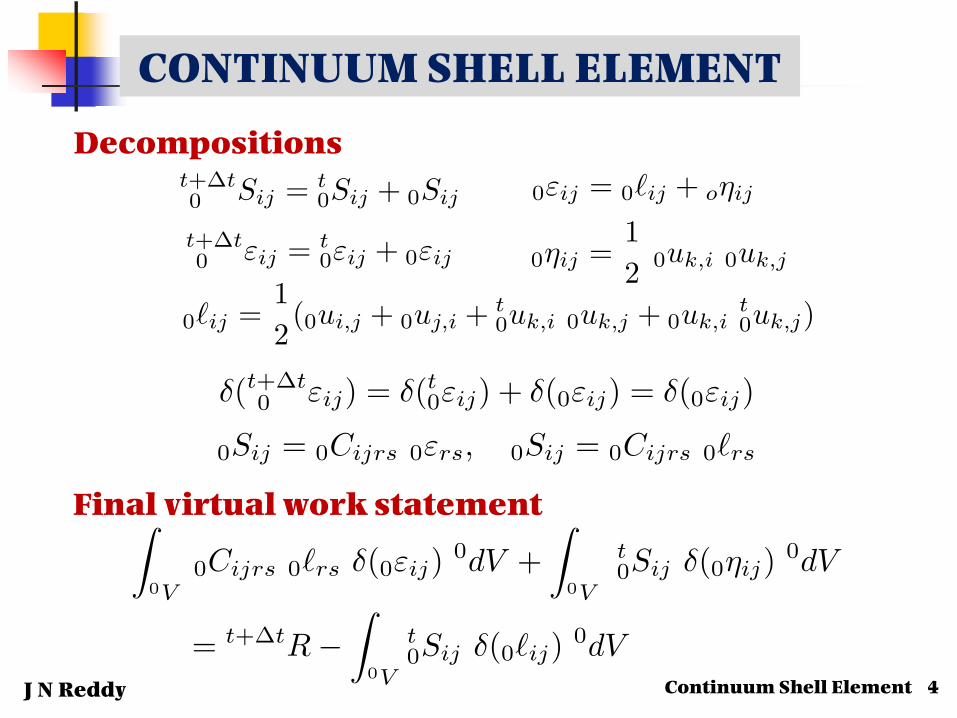
Final virtual work statement
0`ij =1
2(0ui;j + 0uj;i + t
0uk;i 0uk;j + 0uk;it0uk;j)
Decompositionst+¢t0 Sij = t
0Sij + 0Sij
t+¢t0 "ij = t
0"ij + 0"ij 0´ij =1
20uk;i 0uk;j
0"ij = 0`ij + o´ij
Continuum Shell Element 4J N Reddy
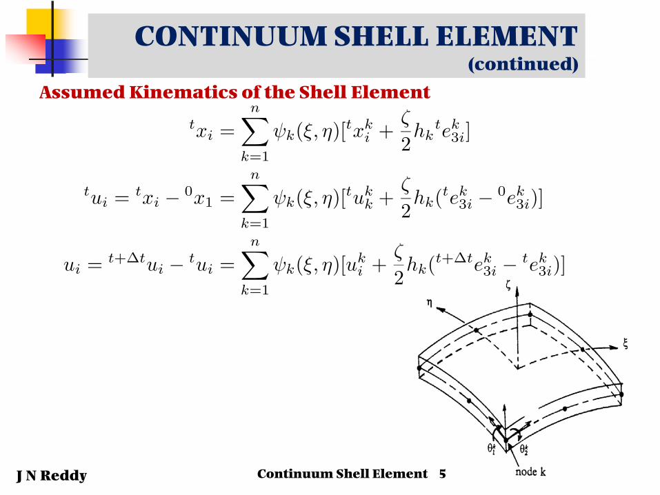
Assumed Kinematics of the Shell Element
CONTINUUM SHELL ELEMENT(continued)
Continuum Shell Element 5J N Reddy
txi =nX
k=1
Ãk(»; ´)[txki +
³
2hk
tek3i]
tui = txi ¡ 0x1 =nX
k=1
Ãk(»; ´)[tukk +
³
2hk(tek
3i ¡ 0ek3i)]
ui = t+¢tui ¡ tui =nX
k=1
Ãk(»; ´)[uki +
³
2hk(t+¢tek
3i ¡ tek3i)]
Continuum Shell Element 6
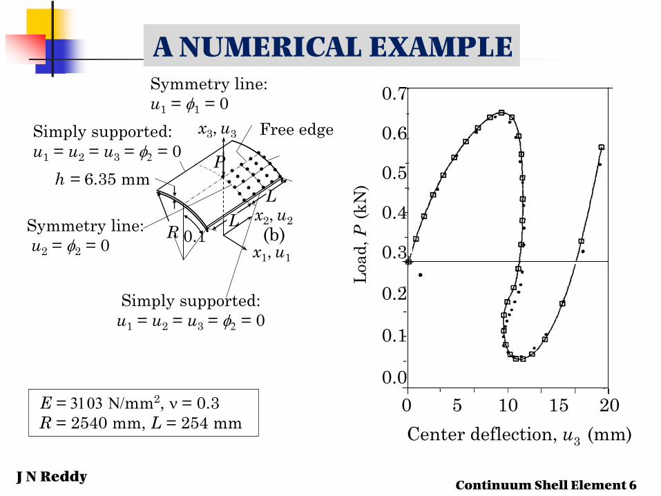
E = 3103 Ν/mm2, ν = 0.3R = 2540 mm, L = 254 mm
(b)
0.7
0.6
0.5
0.4
0.3
0.2
0.1
0.00 5 10 15 20Center deflection, u3 (mm)
Load
, P(k
N)
•
-
-
-
L
Rx1, u1
x2, u2
x3, u3
h = 6.35 mm
Free edge
•••••
••••••••••
••••••••••
Simply supported:u1 = u2 = u3 = φ2 = 0
Symmetry line: u1 = φ1 = 0
Simply supported:u1 = u2 = u3 = φ2 = 0
0.1LSymmetry line:
u2 = φ2 = 0
P
A NUMERICAL EXAMPLE
J N Reddy

POSTBUCKLING AND FAILURE ANALYSIS - AN EXAMPLE
• Nonlinear FE analysis • Comparison with experimental results of
Starnes and Rouse• Progressive failure analysis
a
P
x
y
b
0=w0
u0 constant=w0 0=
∂x∂w0
0=∂x
∂w0
=u0 0=w0
u0
a = 50.8 cm (20 in.), b = 17.8 cm (7 in.), hk = 0.14 mm (0.0055 in.)
24-ply laminate: [45/-45/02 /45/-45/02 /45/-45/0/90]s
E1 = 131 Gpa (19,000 ksi), E2 = 13 Gpa (1,890 ksi),
G12 = 6.4 Gpa (930 ksi), ν12 = 0.38 (graphite-epoxy)
J N Reddy Continuum Shell Element 7
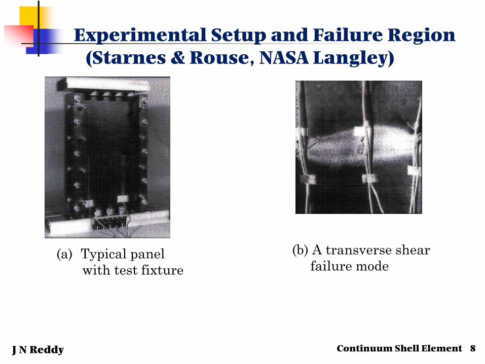
(a) Typical panelwith test fixture
(b) A transverse shear failure mode
Experimental Setup and Failure Region(Starnes & Rouse, NASA Langley)
J N Reddy Continuum Shell Element 8
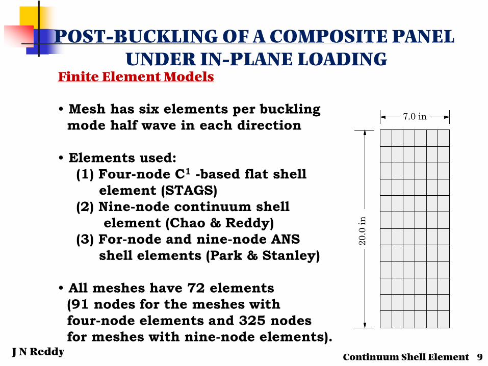
POST-BUCKLING OF A COMPOSITE PANELUNDER IN-PLANE LOADING
20.0
in
7.0 in
Finite Element Models
• Mesh has six elements per bucklingmode half wave in each direction
• Elements used:(1) Four-node C1 -based flat shell
element (STAGS)(2) Nine-node continuum shell
element (Chao & Reddy)(3) For-node and nine-node ANS
shell elements (Park & Stanley)
• All meshes have 72 elements (91 nodes for the meshes with four-node elements and 325 nodesfor meshes with nine-node elements).
Continuum Shell Element 9J N Reddy

Comparison of the Experimental (Moire)and Analytical Out-of-Plane Deflection
Patterns
J N Reddy
ExperimentalTheoretical (FEM)
(b) Photograph of Moiréfringe pattern
(a) Contour plot of theanalytical results
Continuum Shell Element 10
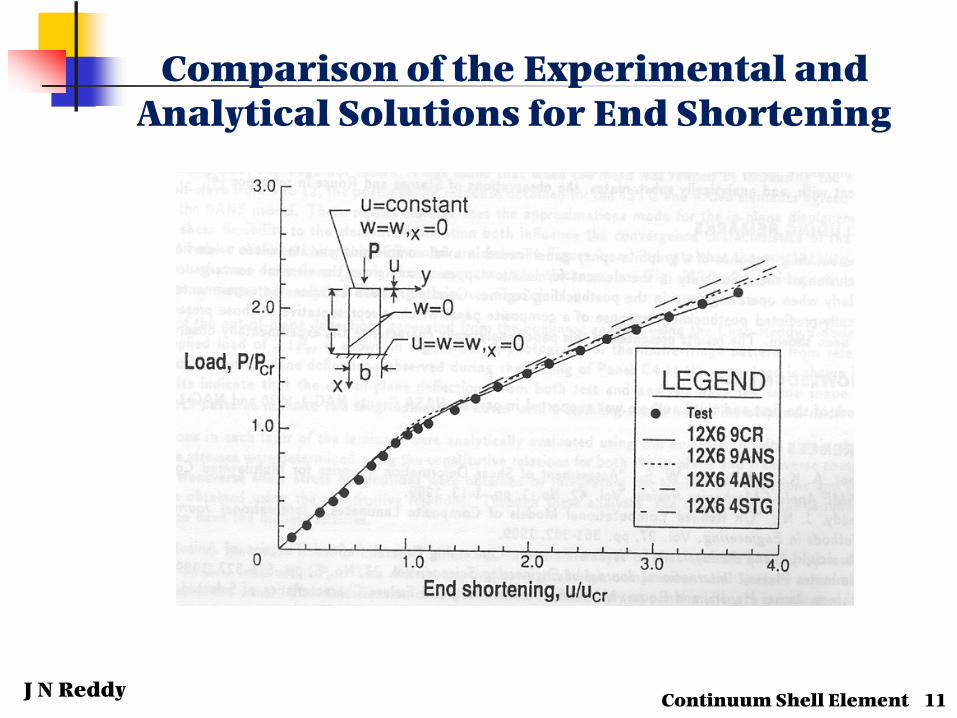
Comparison of the Experimental and Analytical Solutions for End Shortening
J N Reddy Continuum Shell Element 11

Postbuckling of a Composite Panel
0.0 0.5 1.0 1.5 2.0 2.5 3.0 3.5 4.0End shortening, u0/ucr
0.0
0.5
1.0
1.5
2.0
2.5
p,
c
AnalysisTest
0.0 0.5 1.0 1.5 2.0 2.5Maximum deflection, w0/h
0.0
0.5
1.0
1.5
2.0
2.5
p,
AnalysisTest
J N Reddy Continuum Shell Element 12
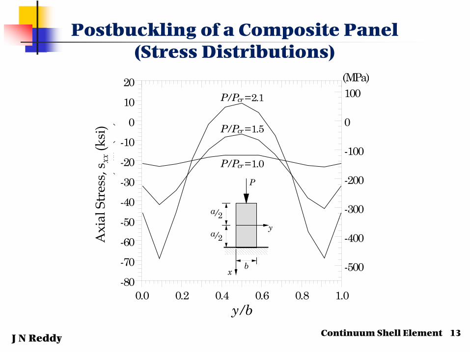
Postbuckling of a Composite Panel(Stress Distributions)
P
x
y
b
a 2
a 2
0.0 0.2 0.4 0.6 0.8 1.0y/b
-80-70-60-50-40-30-20-10
01020
,
xx (
)
-500
-400
-300
-200
-100
0
100(MPa)
P/Pcr = 2.1
P/Pcr = 1.5
P/Pcr = 1.0
Axi
al S
tres
s, s x
x(k
si)
J N Reddy Continuum Shell Element 13
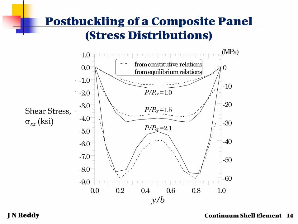
0.0 0.2 0.4 0.6 0.8 1.0y/b
-9.0-8.0-7.0-6.0-5.0-4.0-3.0-2.0-1.00.01.0
,
xz (
)
-60
-50
-40
-30
-20
-10
0
(MPa)
P/Pcr = 1.0
P/Pcr = 1.5
P/Pcr = 2.1
from constitutive relationsfrom equilibrium relations
Shear Stress, σxz (ksi)
Postbuckling of a Composite Panel(Stress Distributions)
J N Reddy Continuum Shell Element 14
Description of continuum shell element(principle of virtual displacementsconjugate pairs, decompositions, approximation of the geometry and displacement field)
Post-buckling analysis of composite panels and comparison with experimental results
(problem description, boundary conditions, fringe patters of the displacement field, post-buckling path; failure analysis)
J N Reddy Continuum Shell Element 15
SUMMARY