TABLE OF CONTENTS 4182

AIVC 11868

MAIN PAGE

T-Method Duct Design, Part V: Duct Leakage Calculation Technique and Economics

Robert J. Tsai, Ph.D. Member ASHRAE

Herman F. Behls, P.E. Fellow/Life Member ASHRAE

Leo P. Varvak, Ph.D.

ABSTRACT

The procedure of incorporating duct leakage into the T-method simulates leakage as an additional parallel section with zero length for each duct section. The assumption that additional air leakage creates additional system resistance is wrong. Leakage always reduces, not increases, system resis­tance. How fan power consumption changes due to leakage depends on the fan performance curve.

Methodology was developed to add duct leakage to the T-method previously developed for both the design and simu­lation of duct systems. It is shown that in most cases the sealing of ductwork is economical. Duct sealing is not recommended when electricity cost is less than 2¢/kWh and sealing cost is greater than $1.5/m2. A simple rule is: the higher the system cost, the greater the need for ductwork sealing.

INTRODUCTION

For the series of T-method duct design research projects, the following papers have been published: "Part I, Optimiza­tion Theory" (Tsal et al. 1 988a); "Part II, Calculation Proce­dure and Economic Analysis" (Tsal et al. 1988b); "Part III, Simulation" (Tsal et al. 1 990); "Part IV, Duct Leakage Theory" (Tsal et al. 1998).

This paper covers calculation technique and leakage stud­ies to determine the economics of sealing ductwork.

There are two applications ofT-method duct design: opti­mization and simulation. T-method duct optimization is based on calculation of duct sizes that minimize the life-cycle cost, including energy, duct, and fan costs. T-method duct simula­tion calculates actual airflows and the fan operating point for given systems with known duct sizes and fan performance. Due to leakage, the actual flow rate is usually less than designed. To compensate for lost air, fan flow is increased by

changing the operating point on the fan curve. It is impossible to manually analyze actual flow due to the distribution of air leakage through a duct system.

A supply system may have places where static pressure will be negative due to the change of air velocity and static regain or static loss and/or turbulence such as that caused by an elbow. Practically, this sucks air in from the outside instead of leaking it out. For practical reasons, calculation of this phenomenon is avoided by assuming zero supply ductwork infiltration.

The technique developed was tested using the sample problem in the "Duct Design" chapter of the 1985 ASHRAE Handbook-Fundamentals (ASHRAE 1 985).

LEAKAGE IN A BRANCHED DUCT SYSTEM

Theory and Calculation Technique

Duct Simulation. The purpose of T-method simulation is to determine the flow within each section of a duct system of known duct sizes and fan characteristics. Incorporating duct leakage means that downstream airflow at each section is different from upstream due to air leakage through the duct walls. T-method with duct leakage incorporates the following major procedures:

1 . System condensing. Condense the branched tree system into a single imaginary duct section with identical hydraulic characteristics. Duct leakage is simulated as an additional duct section connected in parallel to each duct section in a duct system.

2. Selection of an operating point. Determine the system flow and pressure by locating the intersection of the system char­acteristic and the fan performance curve.

Robert J. Tsai and Leo P. Varvak are with NETSAL & Associates, Fountain Valley, Calif. Herman F. Behls is with Behls & Associates,

Arlington Heights, Ill.

THIS PREPRINT IS FOR DISCUSSION PURPOSES ONLY, FOR INCLUSION IN ASHRAE TRANSACTIONS 1998, V. 104, Pt. 2. Not to be reprinted in whole or in part without written permission of the American Society of Heating, Refrigerating and Air-Conditioning Engineers, Inc., 1791 Tullis Circle, NE, Atlanta, GA 30329. Opinions, findings, conclusions, or recommendations expressed in this paper are those of the author(s) and do not necessarily reflect the views of ASH RAE. Written questions and comments regarding this paper should be received at ASH RAE no later than July 10, 1998.

3. System expansion. Expand the condensed imaginary duct section into the original system with flow distribution.

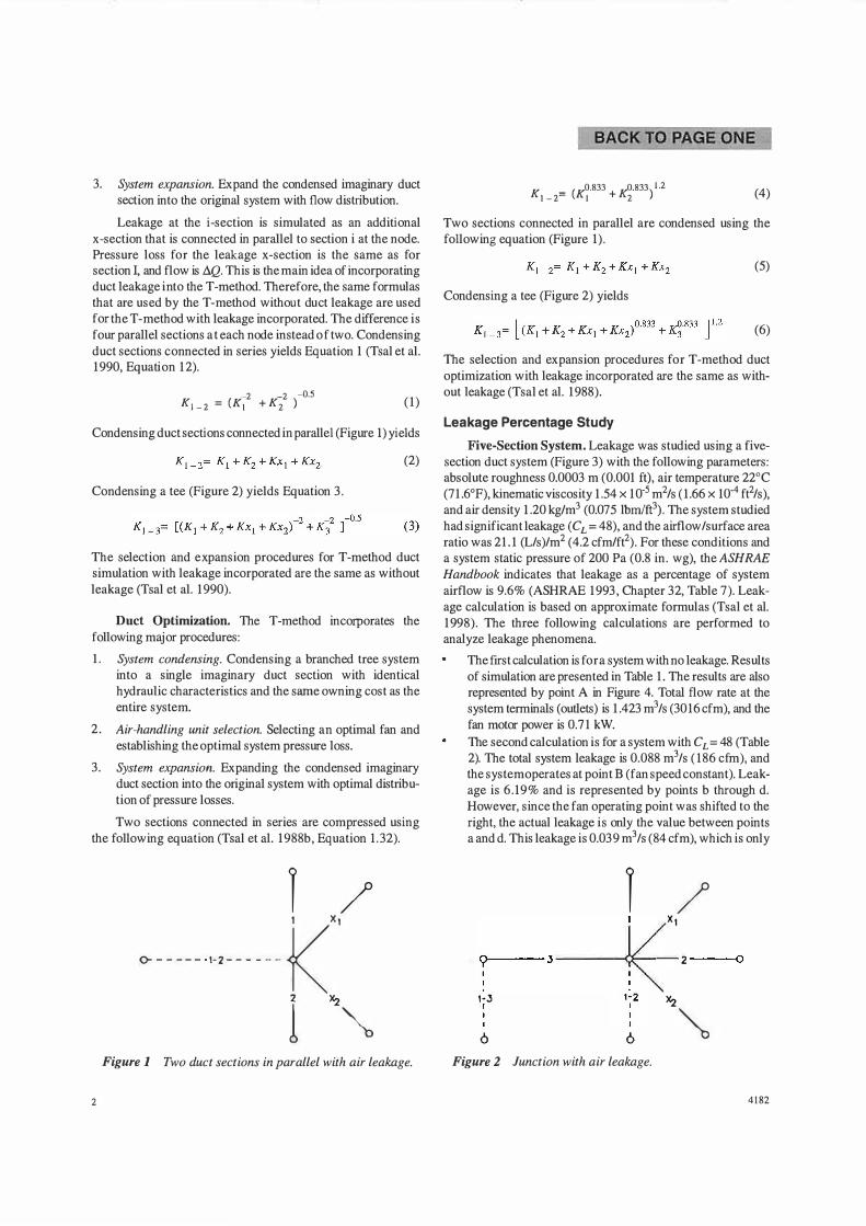
Leakage at the i-section is simulated as an additional x-section that is connected in parallel to section i at the node. Pressure loss for the leakage x-section is the same as for section I, and flow is ilQ. This is the main idea of incorporating duct leakage into the T-method. Therefore, the same formulas that are used by the T-method without duct leakage are used for the T-method with leakage incorporated. The difference is four parallel sections at each node instead of two. Condensing duct sections connected in series yields Equation 1 (Tsai et al. 1990, Equation 1 2).

-2 -2 -0,5 K1-2 = (Ki + K2 ) (1)

Condensing duct sections connected in parallel (Figure 1) yields

(2)

Condensing a tee (Figure 2) yields Equation 3.

The selection and expansion procedures for T-method duct simulation with leakage incorporated are the same as without leakage (Tsai et al. 1990).

Duct Optimization. The T-method incorporates the following major procedures:

I. System condensing. Condensing a branched tree system into a single imaginary duct section with identical hydraulic characteristics and the same owning cost as the entire system.

2. Air-handling unit selection. Selecting an optimal fan and establishing the optimal system pressure loss.

3. System expansion. Expanding the condensed imaginary duct section into the original system with optimal distribu­tion of pressure losses.

Two sections connected in series are compressed using the following equation (Tsai et al. 1988b, Equation 1 .32).

i/ 0------ M------k" 2 �

l � Figure 1 Two duct sections in parallel with air leakage.

K _

(K0.833

K0.833

) l.2

1-2- I + 2 (4)

Two sections connected in parallel are condensed using the following equation (Figure 1).

(5)

Condensing a tee (Figure 2) yields

(6)

The selection and expansion procedures for T-method duct optimization with leakage incorporated are the same as with­out leakage (Tsai et al. 1988).

Leakage Percentage Study

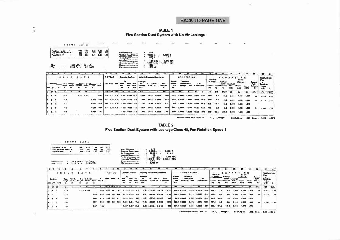
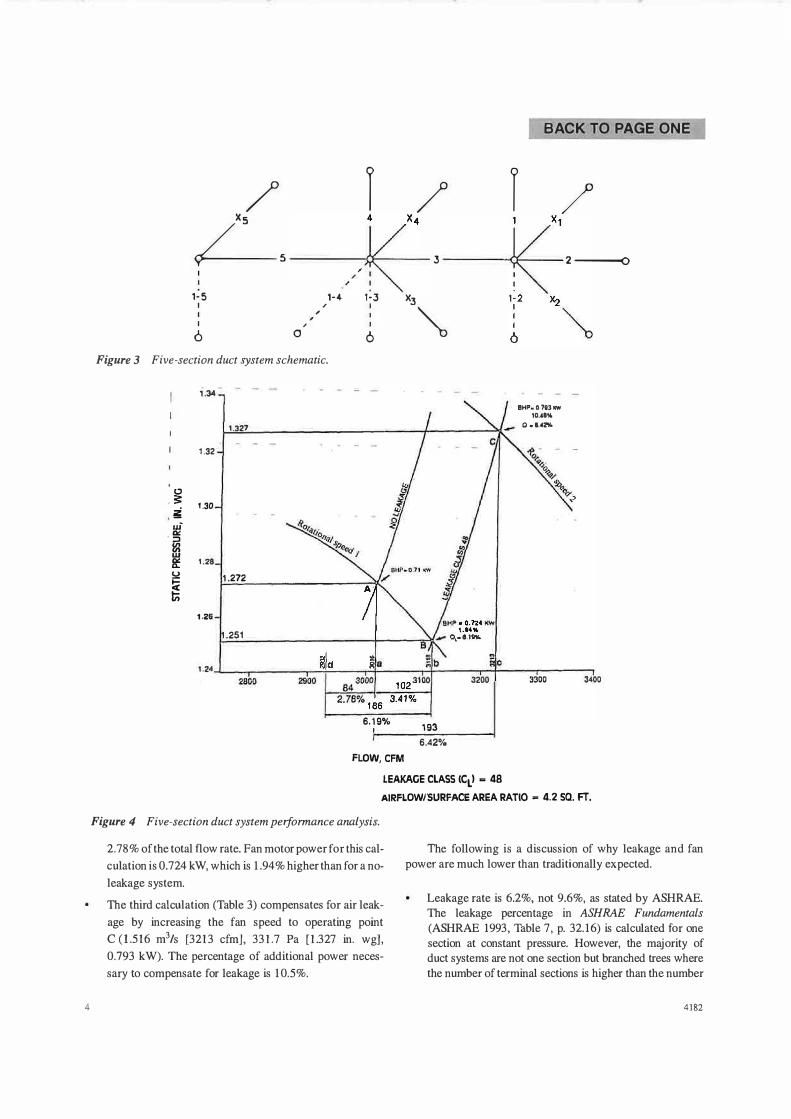
Five-Section System. Leakage was studied using a five­section duct system (Figure 3) with the following parameters: absolute roughness 0.0003 m (0.001 ft), air temperature 22°C (71 .6°F), kinematic viscosity 1 .54 x 10-5 m2/s (1 .66 x 10-4 ft2/s), and air density 1 .20 kg/m3 (0.075 lbm/ft3). The system studied had significant leakage (CL = 48), and the airflow/surface area ratio was 21 . 1 (L/s)/m2 (4.2 cfm/ft2). For these conditions and a system static pressure of 200 Pa (0.8 in. wg), the ASHRAE Handbook indicates that leakage as a percentage of system airflow is 9.6% (ASHRAE 1993, Chapter 32, Table 7). Leak­age calculation is based on approximate formulas (Tsai et al. 1998). The three following calculations are performed to analyze leakage phenomena.

The first calculation is for a system with no leakage. Results of simulation are presented in Table 1 . The results are also represented by point A in Figure 4. Total flow rate at the system terminals (outlets) is 1 .423 m3/s (3016 cfm), and the fan motor power is 0.7 1 kW.

The second calculation is for a system with CL= 48 (Table 2). The total system leakage is 0.088 m3/s ( 186 cfm), and the system operates at point B (fan speed constant). Leak­age is 6 .19% and is represented by points b through d. However, since the fan operating point was shifted to the right, the actual leakage is only the value between points a and d. This leakage is 0.039 m3/s (84 cfm), which is only

i / X1

9 2 0

1-.:5 �

6 6 � Figure 2 Junction with air leakage.

2 4182

_.,. 00 N

w

INPUT DATA

fMftOW', m3/s • 0.12

hn snuura.. tn..WG • 330 Fan llftlcieney • D.75

Cfan ___ _ Plan ___ _

) .

1 • .Ul m31• � Jfl.1 Pa •

• •

1.02 1.42 S2ti 311

a.a o.as

3015 ctm 1.271n.WG

I

I N P U T D A T A

1.12 215

0.13

%.22 202

o.u

RATIOS

BACK TO PAGE ONE -

TABLE 1 Five-Section Duct System with No Air Leakage

MC1tor Ell'ic::l9nq' ·-··--· Absotut. Rougime•-· Air Tempenbn--·-· lA•U. C\ass ···-··-·-· ..... """'"'-··-·-·-··-·-· Kinunmtic V111costtv ••••• Eran. .• ·--··--·-···-······ ----·--···-·-···-··-···

1::11 1i 15

�IMtltt-Surflce

by

1.75 • 0.0003 m • 0.0001 ft

22..DG C • 71.S F •

1..20 mJls • D.D7S 1U1s • 1..scE-Sm:vt• 1.ME ... ft2ll.

..

USO a.110 kW'

i1 '"

v .. DCltJ-Prusurw-Ru1s1:1nce

....... II"

,. "' •• .. D

C ONDENSING

-·

,. is .,. 71 ... .. JO

l X P A N SI H G PruliUN Flaw

"

•nowa An,.. lllnodu &cas

n "

COMPARISON Flow t Sections __ . Duct Rough. D u ct S I it a C-

L8ngt Factor Hlllght Width Dtam. Coeff. Ch2

low Ana V•l. I Frie- Velo- Sur-tlon dty race

m2

Air Friction Sect. V .. ocitr F • ct o r Chanc:btr

mis

Acbml ....... Loss P•

� T•• t..abge Tab.I Coeflici.nts

---Slatk l..eakag9 P•th

Uppe r L.vwer Pra.ln Flaw UPS* Lower Pr.Loss P9. Pe Pa m!I• mlf• .m319 Pa

.. Tmmlnals

Noloa m31s % �- s' s� L---.;: .....-----...----i> c ·� DI DwMIVav - .,. ... " Kt "' PHv � OU Dd Qd

� 14.0 0.254 0.257

12.11

...

O.IO I o.n 0.11 O.!MI 0..255 0..211111 tOI 10.11111 0.0211 0.0211 D.5761 131i.2 D.0000 D.0596 D.0596 o.757 I 136.1 .a.2

0.170 0.65 I 0.24 0.21111 0.161 D.170 0.170 IA t.11 0.020 0.02.a o.4021 112 a.DODO o.01e1 0.0191 D..243 I 136.1 .a.2

O.J20 0.18 I 0.64 0.54 1.201

0.320 0.320 I.DI 11.41 0.0206 D.0206 D.2221

5''-0 0.0000 0..1241 0.0665 D.6451190.1 136.1

D.231 0,65 0.36 0.21 1.27 Q,231 0.231 11.S 12.DI D.0223 0.0223 0.50fl 190.3 0.0000 0.0367 0.0367 D.lSS 190.1 .0.2

33.t 0.000 D.H5 D.1195

29.2 0.000 D.223 D.223

15.2 0.000 D.911 0.918

51.8 0.000 D.506 D.508

0.2 I 0.1115 .0.01

0.2 I D.223 0..02

Cl.2 I 0,506 'A.Ct 16.0

19.1 0.'37 1.50 o.4l1 o.437 n ..l 9.50 0.0193 0.0193 1,C37I 121.D D.DDOO D.1251 D.0791 1.000 l 311.1 fl0,1 200.t D.DOO 1.423 1.423

IN PU T D AT A

Fan 11ow, •:II• - o.•2 Fan Pf9Mlft., ln,WG • 330 Fan .nici.ncy • D.75

Qf•n_,_ Pfan.,... __

1A1t m31s • 312.1 Pai ..

t.G2 1.42 329 311

0.13 0.85

3117 efrn 1.251n.WG

U2 275

0.13

- ··---.a.-----· ------�------------' _____ ___ _________ __._ Airftowtsurrace Rnlo, lhlm2 • 21.1 ' l&IQge -

TABLE 2 Five-Section Duct System with Leakage Class 48, Fan Rotation Speed 1

2..22 ""' 0.12

llotarElncienc)' •m•M­AbsDlutm RaughneH­Alr T•rnperabni.--. l.N.klll'I Cl&H -···-·-·­Air OMr;llJ.----- ·--­KlntrMtic. Vlt;costty._,. a.in.... .. ______ _ Mfan. ........ -_ •• .,.,._. ---

D.75 • D.0003 m • 0.0001 ft

22.00 C • 71.& F ...

t.20 m31's • D.075 l't3l9 - 1.!ME..S rn2ts - t.a£.A lt2h

0.710 0.724 kW

D.00 %,Qsum 1.423 , Qsum • 1.'23 -G.01 %

�- ---.... s ' 1 I • r 10 11 t1 I p ,, n I iii- t7 1.--,.-� JO 2i" Z2 µ ::i:� 1$ 21' :n p 30 :n I �2 ?.l_J I N P U l D A T A RATIOS Dlametar.Suffacs I Velodtr-Pressw-e-Restshlncs

by ·-

C ONDENSING

-

E X P A N SI N G PAis1ure F I o • at nodes Awrmge d nodu &cess

COMPARISON Aow

.. ��--Duct Rough.�� C.. Ffk.. Vel� Sur- Air Friction Sect. Lengt Fllclor Height Wsdth Di•m. Coen. tfon dty face Velocity F •ct or Charachir

Aclaal ....... I.DH Pa

eo.llic .. nts T • • Lnb!illl Total Coetricients

Static L.ukage Path Upper Lower PNlsurm- Aow lJpp9r LOW9r Pr.Lou

T..-mlmls -·

Sec Ch1 Ch2 m m • m 111 m m m2 mis Pl Pa P• mlls mJls m3ls P• m:W. .,.

s sl u: .. .: D .. w c _ I C �MIA V.JV; v ..... K ltn nu � .... .Q!__�

t II

14.D

12.ll

...

16.0

19.11

0..254 D.257 0.80 I 0.75 0.11 D.921 D.255 0.211 14..ll 10.43 0.021119 0.0219 0.5761 129.9 0.0008 0.0595 0.0603 0.758 I 121.l ·1.6

D.170 ll.65 I 0.24 0.211 0,1151 0.170 0.170 &.A 9,61 0.02436 0.0244 0.4031 130.8 D.0004 ll'.JHl1 0.01ts 0.2:M I 128.3 .2.11

0.320 D.111 I 0.62 0.54 1.1'rl O.JZil D.320 I.DI 1l..2'$ 0.0l'DS' 0.0206 0.2221 52.1 0.0005 Q.12'.9 0,0571 0,1451181..2 128.3

0.231 0.65 0.3-t 0.28 1.23 D.1.31 D.231 11.e 11L8i D.02227 0,0223 0.507 1as.o o.ooor 0.DlU D.0374 D.355 111.2 -s.a

31.7 0 009 0,683 0.174

H.5 0.004 o.zzo 0.215

11.5 0 009 0.113 O.IOJ

41.4 0.010 D-.503 D.4M

0.431 1.50 0."37 0.437 27..2 9.64 D.01924 D,0192 1.0381 131.1 D.0025 Cl.12551 0.0!32 1.000 I 312.1 111.2 191.5 0.056 1A11 1.416

•·• 1 0.69.5 -3,04

2..& 0..223 -3.04

3.a I o.506 -z.s7

Alrllowrsurtac• Ratio, u.Jm2 • 21.1 • Laalc•Qll • 6,19%,,Qsum 1.383, Qaum• 1.423--2.ICJ%

4

BACK TO PAGE ONE

/ r / r / L 5 -----,,

,-<�" J ------cF----x-1 2---0

, �

T /,,,_. :, .,\, 6

Figure 3 Five-section duct system schematic.

1.34

1.327

1.32

0 . :;: 1.30 z ,-

uf a.:: ·::i � w a.:: 1.28 a.. !::! 1.272 !;( t;

1.26

.251

1.24

28GO 3200

6.19% 193 6.42%

FLOW, CFM

c

BHP• 0.793 ow lo.1114.

Q •l.•Z'ICo

3300 3400

LEAKAGE CLASS <CLI - 48 AIRFLOWl'SURFACE AREA RATIO - 4.2 sa. FT.

Figure 4 Five-section duct system performance analysis.

2.78% of the total flow rate. Fan motor power for this cal­

culation is 0. 724 kW, which is 1 .94% higher than for a no­

leakage system.

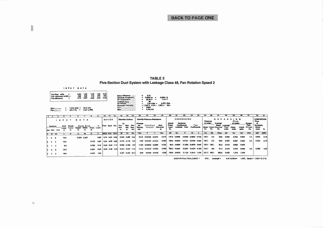
The third calculation (Table 3) compensates for air leak­

age by increasing the fan speed to operating point

C (1.516 m3/s [3213 cfm], 331.7 Pa [1.327 in. wg],

0.793 kW). The percentage of additional power neces­

sary to compensate for leakage is 1 0.5%.

The following is a discussion of why leakage and fan power are much lower than traditionally expected.

Leakage rate is 6.2%, not 9.6%, as stated by ASHRAE. The leakage percentage in ASHRAE Fundamentals

(ASHRAE 1993, Table 7, p. 32. 16) is calculated for one section at constant pressure. However, the majority of duct systems are not one section but branched trees where the number of terminal sections is higher than the number

4182

... 00 "'

lA

BACK TO PAGE ONE

TABLE 3 Five-Section Duct System with Leakage Class 48, Fan Rotation Speed 2

,

INPUT DATA

Fan now, mllt • CU2 Fan ,,_....., tn.WG • 330 F1111 .nid9nCy • D.75

Ill••-­"'""--

2 '

I N

•

p u

1.S11 mJ.ls • Jl1.7Pa •

• •

T D ..

1.02 1.G S2& 311 o.u o.as

3212 cfn1 1.3ZT ln.WG

I

T l!o

1.IZ 275 0.13

•

$edlons Dud Rouigh. Duct Slz!__ C-�--·---Unit Factor �Width Di•m. Coett'. S.c cn1 Ch2 .. .. m m ..

�· u L A M - D c

I • 0 1•0 0.25' D.251 O.IO

' 0 0 Ill 0.170 0.15

J 1 2 1.0 o.320 0.11

� 0 0 16.0 0.231 0.15

5 3 ' 11.8 0.437 1.50

= :m

on ...... - ... -.. __ ._

,. 2

RATIOS

IF11"1f An• Vel.

......

0.75 O.lt U2

D..14 O.ZI 0.85

AkTarnpenlUJL..---1..ubgo Quo --­

Air Donolty. __ ,,_ Klnonutlc lllacoolly .. _. Ehn.-----.... ,,_ ___ _

1l .. ,.

DlMMlmr-Surflice

by Frie- V•lo- SW· - city·-

m m m2

� "" ...

0.255 D..2811 1iU

0.170 D.170 u

0.12 G.54 1,17 0.320 D.320 1.0

O.M 0.21 1.23 0.231 0.231 11.6

0.437 0.437 Z7.2

G.75 • O.CIOCD • • O..DD01 11:

22.DO C - 7U F 48

1.20 ma • 0.075 ft3ls • 1.54E.S 1nVI • t.SSE.... twa

0.145 0.71lkW

.. t7 ,. ,. � 22 � �

Volodf.,,,..._._,.. CONDENSING

.. _ ........ -Air Friction Soct. - Coolll<*1ls To•

V.Oodty Factor Chonocto• I.Ma Le-.ge Tot.I � ... '""' m ...

Yav ... - .. . �

10.r• 0.02115 o.az19 0,175 13'7.I D.DOOI 0.0516 D.DI04 D.751

.... o.o::iu:i 0.0243 o .... 131..1 D.0004 0.0191 0.0195 D.»4

11.13 O.'D2055 D.D20t 0.222 51.D D.0005 0.1250 D.DITI 0.145

1u• 0.0222> 0.=2 D.5DI \H.D 0.0007 o.0367 o.ou• o.m

1.93 D.0112 G.0192 "'"" 131.1 D.0025 0, USI O.OUJ 1.000

AlrftowtSur'f:.C. Ratio, Lt""'2 •

, � Zf .,. 29 "' ,,

E X P A N S I N G ......... Flow atnoclM Avenge lltnodn Ea--..

·sc.tlc Laak1191 Palh Upper Lo.rw Prw•uno Flow Upper Loww Pr.U.t

Po ... ... ml/a m:ll• -· P•

� � �av � "" "" -

1:16.1 -1.5 33.1 0.009 a.m UM 1.5

1:16.1 �s .... 0.005 1..221 0.222 2.5

192.1 13'.1 13.2 0.010 0.940 D.IJO

192.1 ·U 11.3 0..010 0.511 Cl.508 :u

'31.7 112.1 203.0 o.osa 1.516 1.451

ll

COMPARISON Fl-

ot Tennlnela

-a ln:l/a 'Mo

�

0.895 -0.11

0.223 .0.15

0.5045 0.53

22.5 , Lamoe • 6.�%_Qaum 1.US, Cbwn• 1.423•0.12%

or

of parent sections. Tenninal sections always have low pressure. The average static pressure at tenninal sections is the lowest in the system and at tenninals is zero. There­fore, a branched tree system will always have less leakage than one duct of the same surface area and pressure loss. Air leakage can be simulated by a number of small holes in ductwork. Part of the air will be leaked in or out through these leakage sites. This will move the system curve to the right, creating a new operating point on the fan curve. Therefore, the fan will be actively involved in this process by increasing fan airflow and reducing fan pressure. This can be seen in Figure 4 where operating point A moves to point B. How fan pressure is reduced depends on the fan performance curve. Therefore, the assumption that addi­tional air leakage into a system creates additional system resistance is wrong. Leakage always reduces, not increases, system resistance. How the fan power consump­tion increases depends on the fan performance curve.

There is a traditional, but incorrect, belief that in systems where no allowance has been made for leakage, fan motor power increases as the cube of the ratio of the air quantity (AABC 1 983). Therefore, it is commonly stated that leak­age can be compensated for by additional fan horsepower based on the following fan law equation, where Mis the fan motor power and Q is fan airflow.

(7)

Using flow rates from Tables 1 and 2 or Figure 4, the new fan motor power requirement Mis

6.M = (l.1-0.71)100/0.71 = 55.6%.

However, Equation 7 is not appropriate for comparison since the system with no leakage and the system with leak­age have different system curves. The results of the calcu­lation summarized in Figure 4 shows that the actual increase in power is only 10.5%, not 55.6%. Point B on the fan curve (Figure 4) presents the actual leakage rate of 6.2% in the five-section system for unsealed ducts (CL= 48). This does not mean that the design airflow at the tenninals will supply 6.2% less air because the fan curve moves right, increasing the system airflow rate. As shown by Table 2 and Figure 4, the total leakage is 6.2% of which 3.4% is above the design flow rate because, for a constant fan speed, flow increases as the system resistance decreases. Thus, the system leak­age relative to the design flow rate is only 2.8%.

ASHRAE Example. The simulation procedure with leak­age is tested on the duct system presented in the 1985 ASHRAE

6

BACK TO PAGE ONE

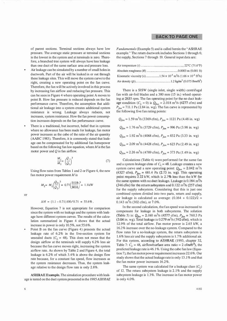
Fundamentals (Example 5) and is called herein the "ASHRAE example." The return ductwork includes Sections 1 through 6; the supply, Sections 7 through 19. General input data are:

Air temperature (t) ..... . . . ............. ......... .... ............... ......... 22°C (7 l.6°F)

Absolute roughness (R) ............... ........... . ...... . . ... ... . 0.0003 m (0.001 ft)

Kinematic viscosity (v) ....... .. ......... 1.54 x 10-5 m2/s (1.66 x 10-4 ft2/s)

Air density (p ) ............................................... 1.2 kg/m3 (0.075 lbmlft3)

There is a SISW (single inlet, single width) centrifugal fan with air-foil blades and a 380 mm (15 in.) wheel operat­ing at 2635 rpm. The fan operating point for the no duct leak­age condition (CL= 0) is Q1,,,, = 2.01 8 m3/s (4277 cfm) and Pfan = 711 . l Pa (2.84 in. wg). The fan curve is represented by the following five fan rating points:

Qfan = 1 .59 m3/s (3369 cfm), Pfan = 1 121 Pa (4.48 in. wg)

Qfan = 1 .76 m3/s (3729 cfm), Pfan = 996 Pa (3.98 in. wg)

Qfan = 1 .92 m3/s (4068 cfm), Pfan = 832 Pa (3.33 in. wg)

Qfan = 2.09 m3/s (4428 cfm), Pfan = 623 Pa (2.49 in. wg)

Qfan = 2.26 m3/s (4789 cfm), Pfan = 373 Pa (1.49 in. wg)

Calculations (Table 4) were performed for the same fan and a system leakage class of CL= 48. Leakage creates a new system curve and a new operating point: Q1,,,, = 2.042 m3/s (4327 cfm), P1011 = 681.4 Pa (2.73 in. wg). This operating point require· 2.22 kW, which is 2.7% less than the kW for the same system with no duct leakage. Leakage is 0.164 m3/s (346 cfm) for the return subsystem and 0.122 m3/s (257 cfm) for the supply subsystem. Considering that this is just one combined system divided into two parts, return and supply, air leakage is calculated as average: (0.164 + 0. 122)/2 = 0. 143 m3/s (302 cfm), or 7.0%.

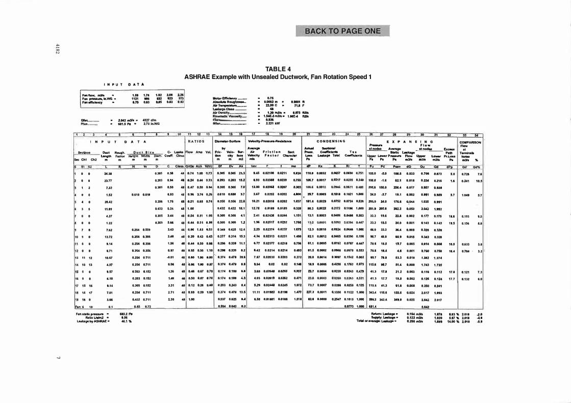
In the second calculation, the fan speed was increased to compensate for leakage in both subsystems. The solution (Table 5) is: Q1011 = 2.160 m3/s (4577 cfm), P1011 = 760.3 Pa (3.04 in. wg). Total leakage is 0.279 m3/s (592 cfm), which is 1 2.9% of the total airflow. Fan motor power is 2.65 kW, a 1 6.2% increase over the no-leakage system. Compared to the flow rates for a no-leakage system, the return subsystem is 1 .6% less air and the supply subsystem is 1 .7% additional air. For this system, according to ASHRAE (1993, chapter 32, Table 7: CL= 48, airflow/surface area rntio = 2 cfm/ft2), the predicted leakage rate is 46.1 %. Using the cube fan law (Equa­tion 7), the fan motor power requirement increases 22.6%. Our study shows that the actual leakage rate is only 13.1 % and that the fan motor power increases 16.2%.

The same system was calculated for a leakage class (CL) of 12. The return subsystem leakage is 2 . 1% and the supply subsystem leakage is 1 .3%. The increase in fan motor power is only 4.0%.

4182

� 00 "'

_,

TABLE 4 ASHRAE Example with Unsealed Ductwork, Fan Rotation Speed 1

IN PUT DATA

Fanflcrw, � . 1.11 1.71 1.12 Fanpruaun.ln.WG • 1121 - m Fon-ncy . t.n o.u us

-.. __ . 2.IM2..slo • .szl -,,, . ..__ . A1.5Pa • 2.nln.WG

' 2 l • 5 • 7 •

I N p u T D " T "

Duct t 11•

2.0I 2..K m ST3

o.u 0.11

• 10 11 IJ ,,

RATIOS

c- Laab Flow Alu Vet.

........ Blidooicy -··-­- R .... -.... AWT--·-1.abgoC.U. __ Alt Donal!y __ _ -111acaolly_ Ban----­------

• " ..

DUmntr-Svrflm

Oy Frie- V•la- Sw-Sections Duo1 Rvugh.

........ Fac&or HitlCll"ll i'&lii) � Co.ff. c:a..u - clly -Sec Chi Ch2 m

SI "2 L

� 0 0 U.31

1 • 0 2'.71

I> 1 2 1.n

• • 0 1.52

5 • 0 2U2

I > s 11.lt

' 0 0 ur

I 0 0 1.22

t 7 I 7.52

10 9 0 1J.72

11 • • 1.1'

.. 0 0 1.71

,, ,, 12 10.'1

" 10 13 ... ,

,. 0 0 1.57

" 0 0 S.10

" 15 11 l.U

• 14 17 7.01

" 11 0 l.H

!Fons 11 0.1

Fan static prusuni •

RatioUWm2 • Laaklge by ASHRA£ .

m m m

.. " w

D.510 0.111

0..254 0.559

0.254 D.305

D.254 0.356

0.254 0.156

0.254 0.711

a.2sc 0.111

0..203 0.152

0.20J D.151

o.m 0,151

0.251 0.711

0.432 0.711

o..cs 1.n

A5.2 Pa ..., ... 1%

m

D c

o.:105 ....

0.2111 O.IC

O.:t05 0.50

1.13

O.SSI 1.7'

D.432 0.2C

O.JOS 3.11

D.305 5.H

3 ...

>Al

1.51

0.17

..0.01

0.00

1.l6

UI

l.31

2.11

2.30

...... •

"' o.u t.oo o.n

... o.2' o.aa o.s•

41 0.•7 0.5D O.M

" D.H :S.74 0.11

u 1.51 0.11 0.71

&1 1.oa

" a.u o.s1 1.05

Q D.4& Ul1 0.15

" D.tl 1.IJ e.SJ

" 0.20 o.u 0."5

a OM 0.50 D.11

'8 D.55 0..50 1.1D

41 O.IO 1.00 a..IO

41 'o.K 1.IO D.17

41 a.a 0.11 0.10

.. 8..50 D.f7 I.TS

.. D.12 IUI OM

41 O.lt O..SI 1.11

... 1.00

m m rn2

... ... ....

D..305 0,305 21.l

1.203 0.203 15.J

0.305 0.305 7.0

0.110 I.Al u

US& O.SSI 22.1

o.•u DAU 11.. 1

0.305 f.305 •.1

D.305 O.lOS 1.l

o.Kt o.m 12.4

0.277 0.314 19.3

0.296 0.331 11.1

0.2H 0.»9 1.2

.. . 0.:114 •.• 71 20.1

0.:11• 0.•78 I.I

0.17' 1.119 I.I

0.174 0.111 u

D.ZOJ 0..243 ...

G.J74 1.471 13.S

D..537 a.a25 I.A

0.551 0."2 1.2

•T

D.75 • o.oau m • l.DOOt fl

21.DO C • 7.1.1 F ...

t.a rnst. • ...,, fDla • 1..uE..Srn21s• ,.HE... ftJls

.... 2.221 kW

II ,, ,,. .. Z2 2l 2• Z> " Z1 21 n )0 'I u ll ...

Velodt:y�aure-Rffh.tanc1 C ONDENSING E X P A N SI N G COMPARISON

,._,,,.. Alt Frlctl en Seel.

Voloclty F• c:tor Cllu>oter mis ..

vov r ""'

1.45 D.021• D.0211 1.121

1.93 O.IWU 0.023' 0.755

11.00 0.020ll 0.0207 O.J03

2.C7 O.H02 0.021D2 .....

10.21 0.02011 0.0202 1.ID7

11.71 t.1111 0,0119 CUD

2A1 O.Ol'38 0.0144 1.151

1.M o.02511 a.om 1.755

2.29 0.0237' 0.0217 1.m

4.3' 0.02S13 0.0231 USO

S.71 0.02171 0.0211 0.751

U2 0.021, 0.0214 0.493

7 .17 0.020JS 0.020J 0.272

1.60 0.02 0.02 ._,.

J.CI O.D2UI D.DZSS D.SST

•.OS 1.DK1t 1.0212 0."71

S.2t 0.02111 D.0215 1.DJJ

11.11 0.01111 0.01H 1.A71

l..51 D.11&11 1.0111 Ul11

......... Flaw � ......... - �Awn1ge al nodes ExcOoo .. ....... �· .... ho Statl� t..Up Patil Termlnala

Laolalgo TOlal � ... ...... Pa

... ""

110.D O.DOJ2

100.7 0.0017

100..1 1,0010

n.1 o.oon

m.1 OJ10211

11..S O.ICl22

1J.1 l.I003

t,>;-1 0..0001

1�3 0.0010

U.1 0.0012

H.1 D.CI005

11.5 0.0002

20.0 0.0014

11.1 G.0005

22..7 Cl.GOO.a

D.O O.OOOS

73.7 0..0007

U7.J 0.0011

12.1 1.0000

� ....

a.our o.oc90 a.1st

D.0217 0.023$ 0.2U

o.°"' 0.0111 OMG

0.1111 0.1121 1..DDC

o.1752 1.on' 1.520

0.2172 0.11K 1.IOO

o.Mlti o.o.ui o�

O.Mtl 0.0:n4 O.MJ'

0.092' o.ocu 1.000

0.0465 O.G3M 0.111

0.1712 0.0117 .... 7

D..DHI 0.0970 0.553

D,JOlf D.15'2 0.802

um o. 1ru D.175

o.02Jt a.ow o .. nt

UJIO 0,02<3 O.lll

0.0211 0.0255 0.12$

l.1UO 0.1112 1.000

0�7 0.1013 1.000

0.0773 ,_

Upper Lowt:r Pruan Po Po Po

rU Pd �"

105.0 -4.0 1Dl.5

1DS.O -1.S 12.1

..... 1115.0 25U

24.0 -5.7 11.1

-· :au 171.1

2'1.t ZOU 31:U

ll.J 15.1 22.1

n.l 19.5 21.0

.... ll.l lU

SU ... 0 ....

11.1 11.5 11.7

71.1 1U 4.1

"-' 71.1 53.l

115.1 N.7 SU

'1.J 17.1 21.2

41.J 17.7 11.5

115.1 au 11.1

J.&3..4 115.1 155.f

.,., J43.4 -··

111.A

R.tum: L..b99 • """"" laolalgo •

Total or avwaea: L..kap •

Flow "-' - 11131•

nu �

0.033 0.708

0.011 o.n.

0.011 0.157

0.002 0."1

o.oaa 1.0l5

0.050 2.0Q

0.002 o.171

0.001 0.1'3

0.009 0.321

D.015 0.3'3

0.005 0.114

0.001 D.700

0.011 1.112

o.ooa 1.7 ..

0.003 0.111

l.D02 0.121

O.OOI 1.250

0.024 2.017

0.025 2.0C:Z

2.0Q

D.114 m3l1 O.t22ndls

0.:ZHndls

'-- Pr.i.-o -- Pa -· %

"" Ocr �

D.11.J 5.0 0.721 7.1

0.211 1.1 0.2'1 1D.5

O.UI

O.NI s.r 1.041 S.7

O.H1

1."2

0.175 11.1 0.193 ....

D.IC:Z 11.5 0.151 I.I

0.120

0.321

O.IOI 11.5 0.IJJ ...

0.751 11.4 0.7U ' l.2

1.174

1.ns

0.112 17.1 0.121 7.3

D.124 17.7 1.131 1.0

0-2'1

1.ltJ

2.017

1.171 Ul "' 2.011 �.O 1.120 UT "' 2.011 .u 1.IH 14.00 % 2.011 -5.1

00

;'.':; 00 N

BACK TO PAGE ONE

TABLE 5 ASHRAE Example with Unsealed Ductwork, Fan Rotation Speed 2

I

IN .. LIT DATA

Fan now, mSla • t.51 F•n pnt.aU19, ln.WG • 1'Jt Fan .nkMcy • D.75

ar.n-- • :Z.1H rnJl'I • PfatL-- • 71G.l ,,. •

2 ' • • .

I N p u T D A l

1.71 1.12 IH UZ o.u 0.15

'5T7-:S.041n.WG

I

A

Dud buct. Slat

2.H 123 D.U

I

us m

O.ll

,.

C- ......

" ,, ,,

RATIOS

Fkrw' NH V•I.

Motor Br1c11ncr-­Abaol1111t Rough,_._ Air T•mpe,.tura __ LMUpCS.•--­Alf;Donslly---­��-Efan.--·---lllfan__ ___ _

,. •• ,.

Dillmetw..SUl"fa�

by Frie- Velo- sur. - lto<ogll. unga, '·- ... iiM ....... DilmO COl'ft. Cini tion city ,. ..

s.cCM Cl1Z m

$1 51' L

' D D :ZA.JI

z 0 • 23.TT

' 1 z T.32

� 0 • uz

� ' • zuz

� 2 5 11.n

1 0 • 4.ZT

' • 0 1.ZZ

' T • 7.IZ

10 • 0 1J.12

11 • • •�14

12 0 0 l.T1

13 11 12 11.17

1.t 1D " UT

ts 0 0 1.57

11 • 0 l.10

1T 15 " 1.1•

II t4 1T T.ot

11 11 • . ...

fin I 1S 0.1

Fan atatlc pr11aaun1 • Rollo u.irnz • t..aklige by A9�E •

m m ..

M .. ...

0.510 0.610

D.2SC D.551

0.254 D.JOS

0.254 D.l5&

0.254 0.356

0.254 G.711

0.25-4 0.711

D..203 0.152

D.203 D.152

l.l05 0.152

0.%0< O.T11

0.432 D.711

11.45 o.n

OIS.Z I'll

I ...

41.1"

..

u ...

IU05 UI

D.202 O.M

o.sos 050

1.13

U.JSS t.7' u.w •.:z•

0.205 ....

0.305 !!Ii.II

3.A3

....

1.56

UT

-G.01

O.OI

1.3'

,_.,

121

1.11

2.00

•

41 O.T• UO 0,7'

41 0.24 OM t.5l

OI UT 0.SO 0.8'

41 t.K 2.T• O.%S

.ca I.St 0.51 0.74

a 1.00

" o.s. 0.51 1.CKi

.. '·" G.51 O.M

oll D.K 1.U 0.53

.. 0.%0 ..... us

41 OM o.su o.n

.. 0.55 0.50 t.10

&II D.ID 1.DO O.ID

., 0.17 1.DO 0.17

'8 I.tr 0.17 0.70

41 Ut O.OT O.TT

.. o.u 0.2' ....

OI O.lt 0.51 1.TI

41 t.DO

m .. mZ

� "' ...

U.305 0.305 ZU

O.ZOJ 0...203 U.2

0.305 O.l05 T.O

UtC Ull 2.1

0 ..... UK ll.I

0.'32 0.432 15. 1

D.305 UOI ...

D.JOS O.l05 1.2

D.M9 D.425 12.4

D.277 0.314 15.S

0..296 O.S39 11.1

0.216 0..339 1.2

O.l74 0.479 20.I

D.37"' 0.471 ...

0.11• D.1H ...

0.11' o.1n u

0..203 o� . ..

un o.m tu

0>37 0.1125 ...

·- 0.1-U 0.%

,,

1.75 • D.DOU m • l.OD01 ft

22.DQ C • 71.S F ..

1..20 m3l9. 1.175 � • 1.s&E...Srn'J&• t..llE-4 ft2la

D.125

Z.151 llW

11 .. ,,, ,., 22 2l ,. :I> " ,, 21 ,. "' .. n ., .. Vtlodty-Praauni�eMIClna CONDENSING E X P A N SIN G COMPARISON

A..,.ge Air Frli;tlon -

Volodty F•clor CN'"-.W• m

Vu r ....

10.00 D.UI 0.021 UZI

1 .:u o.02377 a.one 0.755

t:US O.OZOCZ 0.0:1111 O.l03

uz 0.02004 o.oz UGO

tD.79 0.02011 o.ozot t.m

14..11 0.118"' G.01H 1.m

u1 o.ouot o.o.u1 1 .. i51

2.12 1.02"6 0.02•'1 l.TSS

2..46 o.02u1 o.om 1.175

U3 0.022tT 0.022 U50

7.%1 0.021.. 0.0217 0.756

1.15 D.D21J1 a.ozu Ul2

1.14 0.0202' O.DZOZ o.zn

to.n o.otn2 o.otn 0.14'

�- 0.12G'l:S 0.0211 I.SST

UJ 0.015H 0.02' IA'1t

$.SJ ·� D.02'2 un

11.TT G.11115 O.OIM UTT

UI 0.01Ut 0.0111 1.Stl

3..U 0.0202$ 0.D2tlZ 1.oa2

......... Flow -Actual -· .. .- Aw,.ge .......... -· .. ...... . Codi!:- TH Static.__..,.. Lou 1.uu111 lotal Cod"idonta Up,... L._ p.....,. Flow Uppor Pa

� It>

12.J.O D.D03Z

111.2 l.OD17

U1A 0.0010

D.2 l.IOG3

202.1 l.DDJG

H.l 1.0023

1!U 1.0002

1!1.. 0.0001

1U 0.0009

59.1 D.DG12

H.2 0.0006

,.., 0.0002

22..5 0.001Z

11.0 0.0005

Zl..2 1.000.C.

MA o.ooo:z

U.2 0.-0

ZS/1.1 l.001t

cu 0.0000

P• I'll P•

K llt "" � . ....

O.OCST 1.- D.Tst H6.T .u 115.0

1.0211 D.023S 0� 111.7 .a.s II.%

O.- 0."'7t OAMl 229.1 Ul.7 215.1

e.1111 0.1121 1.oaa IU .&.I 15.1

0.0752 O.D725 0.520 lll.1 .... 197.J

0.217• 0.1117 1.000 1zs.s m.1 _,

O.o.&15 D.CMll O.SSS 17.2 1.1 I.I

O.Ol!IJ O.OJM IM7 1T.Z u 1.3

O.otJA O.DMI t.000 23.5 ,..., 22.1

O.DC'5 0.0311 0.1!1 H.T ZT.I ....

0.0712 D.0711 1.'47 IS.2 -3.1 17.1

o.- o.imt D.552 IU ·U I.I

1.3097 G.15'2 t.I02 H.T IU 35.1

UZZS 0. tTU I.ITS 106.2 IT.J JO

11.0Zlt O.OW D.A71 21.2 ... 10.t

o.0'2'0 o.om u21 Zl.J 1.t t.I

D.02" 0.0255 UZS tou 23.0 U.7

1.1:131 0.1121 1.100 "4.1 n.1 125.1

D..1547 a.1au 1.000 43£.t J12.1 m.1

O.OTT3 1..000 7I0.3

Retum:L..-kl1119• Supply.� ... -

Tota.I or •wnp: t.bge •

- -

... ....

..... ua

D.019 u•T

0.011 1.012

D.001 t.o.t7

D.04I t.M5

t.OS. 1.llO

0.001 0.111

0.000 D.155

O.Otl< US!

0.012 D.SU

0.005 0.153

D.002 UOI

a.a" UTT

OJlllS . ....

0.002 l.tll

D.OOt 0.1M

D.OOT G.28'

1.021 1.135

D.OZT 1.llO

1.t&O

O.IT•rn!lo 1.1a.c rn3la 1.2n,...

..... T-la i..-r Pr.U.. -- ... rn!I• "

Od ...

D.7'2 u o.na :u

0.221 z..s 0.2•1 ...

t.M3

t.MI ... 1.NI O.l

1MT

1.10I

t.llO 1.1 0.113 1.1

1.15' 1.1 0.156 t.3

O.:IU

a.ssz

D.MI 3.1 0 .133 ..z.•

0.006 1' D.TM �2.1

t.AU

1.MZ

1.121 2.1 0.121 ..,_,

l.1ll 1.t 0.12Z .....

1.%51

1.11•

1.U3

1.111 UI % 2.011 -1.1 1.0$1 .... .. 1.011 t.7 L011 12.11 1'. J.011 0.0

' s s eattle. >oiral Duct ,._ ....._-� r----_ � r------_ ----------., ·11----._ -r----

r---.... � t------ ------............___ --------- -----

----- ---...._, h-....._ r---.. ---

-----.__ ............___

_, � ..

.... � .. 1,00 , .. Sealing Cost, $1m2 200 . ...

-•- OCM = L ..... OCM=3..._ OCM=5....,_ OCM=7-+- OCM=9

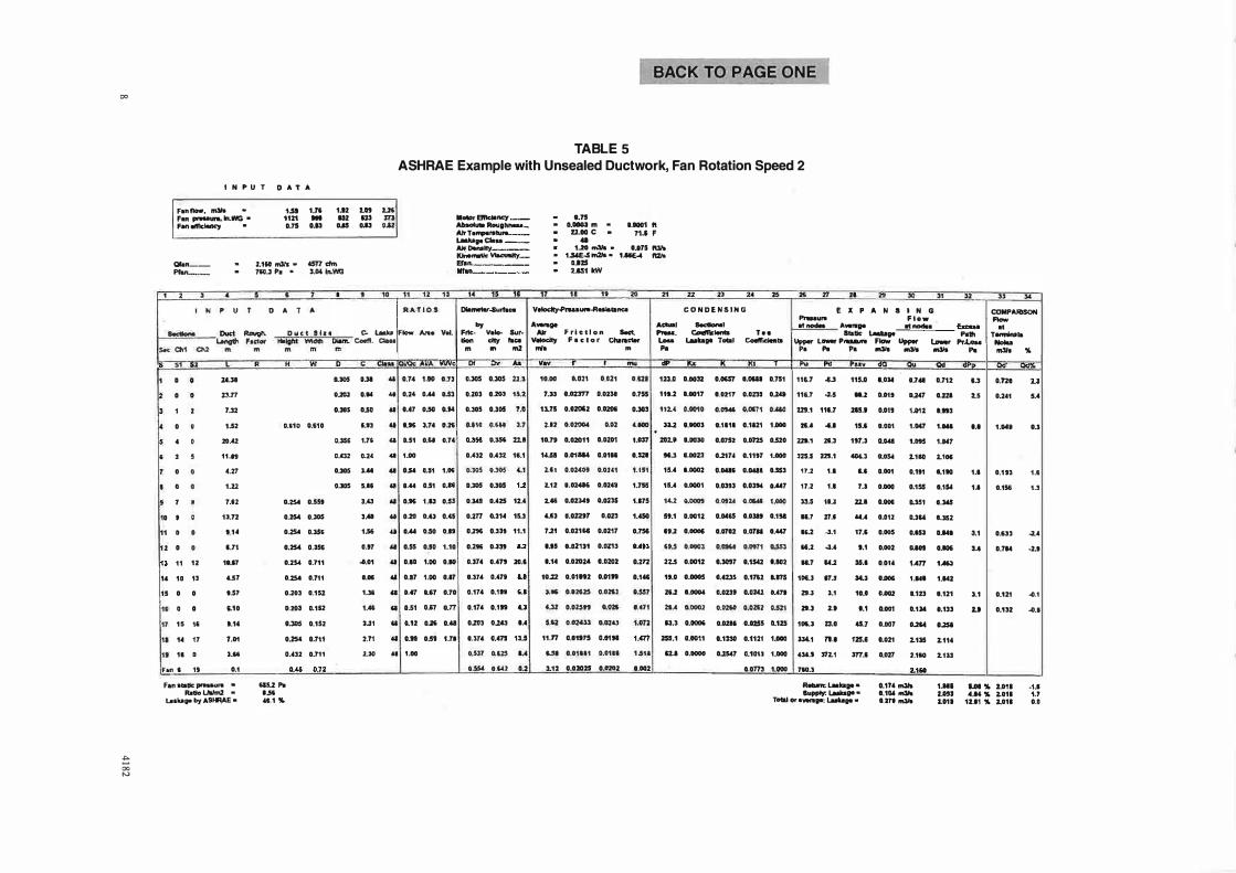
Figure Sa Parametric economic study for Seattle and

galvanized ductwork.

,____

... ....

Sea11lc Stainless Duct

1.00 !� Sealing Cost, $1m2

200

-- OCM= L..... OCM=3-.... 0 CM=5....,_ OCM=7-- 0CM=9

.

Figure Sb Parametric economic study for Seattle and stainless ductwork.

Duct Leakage Economics Study

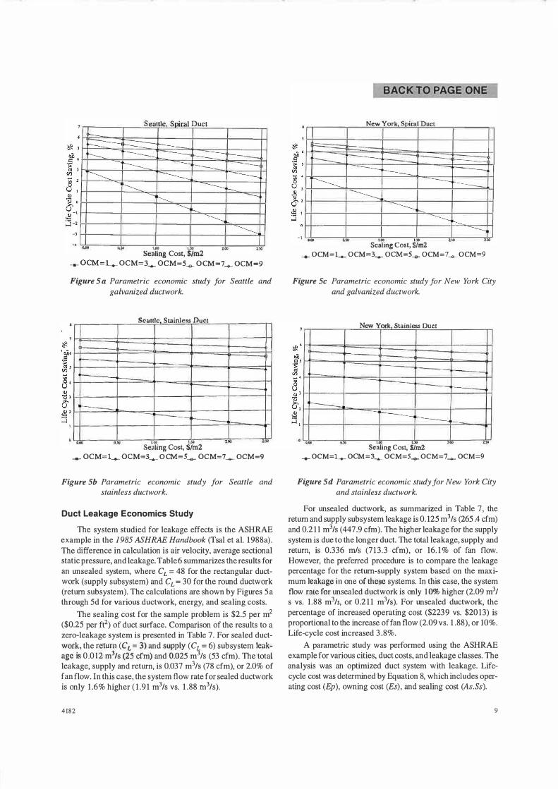
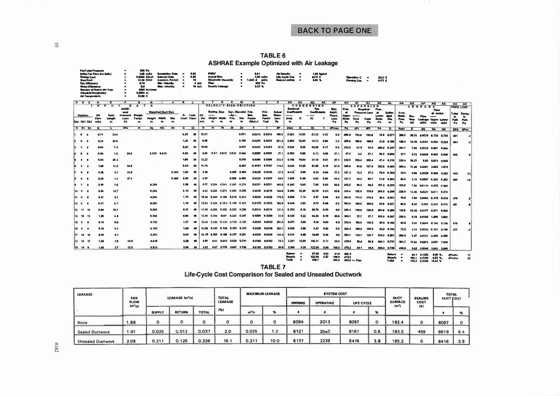
The system studied for leakage effects is the ASHRAE example in the 1 985 ASHRAE Handbook (Tsal et al. 1988a). The difference in calculation is air velocity, average sectional static pressure, and leakage. Table 6 summarizes the results for an unsealed system, where CL = 48 for the rectangular duct­work (supply subsystem) and CL = 30 for the round ductwork (return subsystem). The calculations are shown by Figures Sa through 5d for various ductwork, energy, and sealing costs.

The sealing cost for the sample problem is $2.5 per m2

($0.25 per ft2) of duct surface. Comparison of the results to a zero-leakage system is presented in Table 7. For sealed duct­work the return (C1., = 3) and supply (C� = 6) subsystem leak­age is 0.0 1 2 m3/s (25 cfm) and 0.025 m Is (53 cfm). The total. leakage, supply and return, is 0.037 m3/s (78 cfm), or 2.0% of fan flow. In this case, the system flow rate for sealed ductwork is only 1 .6% higher ( 1 .9 1 m3/s vs. 1 .88 rn31s).

4182

BACK TO PAGE ONE

. New York Sniro L Duct

r--_ �

------r--. -

----------- -r------------

----------------;..._

------I . ., .... '-"' , ... "" llO

Sealing Cost, S/m2 - 0™=� 0™=� 0�=� 0™=� 0™�

Figure Sc Parametric economic study for New York City and galvanized ductwork.

New York Stainless Duct

�

-

�--- -� .___ �

... .... . ... . .. . .. "' Sealing Cost, S!m.2 -- OCM=l-.- OCM=3-- OCM=S ........ OCM=7-- OCM=9

Figure Sd Parametric economic study for New York City and stainless ductwork.

For unsealed ductwork, as summarized in Table 7, the return and supply subsystem leakage is 0. 125 m3 Is (265 .4 cfm) and 0.2 1 1 m31s (447.9 cfm). The higher leakage for the supply system is due to the longer duct. The total leakage, supply and return, is 0.336 mis (71 3.3 cfm), or 16.1 % of fan flow. However, the preferred procedure is to compare the leakage percentage for the return-supply system based on the maxi­mum leakage i n one of the e systems. In this case, the system flow rate for unsealed ductwork is only 1 0% higher (2.09 m31 s vs. 1 .88 m3/s, or 0.2 1 1 m3/s). For unsealed ductwork, the percentage of increased operating cost ($2239 vs. $2013) is proportional to the increase of fan flow (2.09 vs. 1 .88), or 10%. Life-cycle cost increased 3.8%.

A parametric study was performed using the ASHRAE example for various cities, duct costs, and leakage classes. The analysis was an optimized duct system with leakage. Life­cycle cost was determined by Equation 8, which includes oper­ating cost (Ep), owning cost (Es), and sealing cost (As.Ss).

9

0

....

o;; N

A

F•T.WP......,. ...... , .. ,..,.. ... Mt.J ----.... _,. -­................ ,.,v .. -­»T...--.

• c D I N •

• u 1 a

...... .....

... .. t.11 "'3111 � ...... .

.... � � ..... .. U.. IJ#lnZ �....w .

..,. - -u -·-

- -.... ..

2lll .

a n ' J • l A

-- -

.

I ... ....

.. . ...

.. ...

I

BACK TO PAGE ONE

TABLE 6 ASHRAE Example Optimized with Air Leakage

l'WEF -----...... .._

u . w

Ut .... .....

1ME:-I lflZl9 ... ..

. ... "

x y Vt Lw wj TT •:SIZ.IE ... JI: IC TI U'fll

-· - ...... - Mo- Fri<·

·­u. cp c. • -....- .

. ,. &C

uo -141' ' .... ..

"" Al c u .. u t. N • I N D

-� , .. - �

..

.... ... ..

- · _ ...

AW .. IU

.... . 1177 '

AK E J. P .4 M • • O N

-· - --

AL

.. .......,,. Loas Ill -

....

.._. -rd Air """ .... .- ...... c. .._ "" - .....,_ - - -. . - -- -.. -· -- ,,_ - -

.... ._., ..... ·- - -J:s4.=: ai1 Q2 ..st• .. .. .. .. ..

• •• 5.2 a . ..... " "' ...

, • • 1.71 14.4

� • • .... ZJ.I

� t • IM r.>

� I I OM u zu D.11G G.110

• • .... ....

• • • t.U t1.I OU

. • I ..,. u 2U

• 0 I .... u Jl'A

• 1 I .... .. .....

•• • • . ... 1J.7 .....

ti • I . ..., . .. .....

u • • ...., .., UM

I<> t1 t2 OM .... .....

11'1 11 1J UI ... .....

k• • • ..,, ... 1.152

11• • . .... ... 1.1'1

h'r 11 ff ..... l.t l.20l

u ,. 17 t.11 1.1 to.a •-'11

II ti • .... "' , .... .....

LEAKAGE

F AN Fl.OW l�'/:11)

SUPl'l.Y

None 1 .88 0

Sealed Outtwork 1 .91 0.025

Unsealed Ductwork 2.09 0.21 1

.... ..... ..... v.a.. Height Widl'I ffE. - - ·- .... .. .... .. . . . ....... T ... ..

"' r v K w m � ' -

IZI .. 1U7 1%11 Dn13 0Jt21J 1n.1

t.2 JO .... D.190 o.am D.OZ3!1 ZOU

.... .. ..... ..... , l.nol •.a20> .....

l.S:Z .. ..., 0.61 G.111 UfCI I.IA o.moo 1.moa 21.t

t• " t:UZ ..... 0.DZlll l.D20I .....

.... JO tt.1t ... .. 0.1117 1..1117 .....

...... t.N "" ..... UK l.»t OJlZZI IJ1221 ., ..

..... .... " .., I.JOI I� o•m 1.om ....

t.21 .. UJ O.lM u.&1 11..20' IZ7t DJt221 1Jt221 .....

.... .. Lil 11.ll& OZ/� 0.l'W IJ.2:M. D.Cl211 O.D211 ....

t.n II 11 . .U I� II.HO 1.210 0..Ut D.11221 l.DZZI tn.2

t.1t .. t2.J.j O.:&U 0.1H· l.t• t.n1 IJZ.U l.GZJ2 tlU

I.ti .. 14.ft O.lU t.2A UQ l.Z. D.n14 1..1214 Ul.2

.... .. tUC O..l:U I.NJ 0..3.M l.::lllJ o.moa •.moa JUI

t.27 .. 10.AG IUD G,;S:U LW L11:J l.Jl25S D.Jl2.U ....

.... • H.ft I.tu I.tu UH L1tl l.D2SI 1.1251 .....

..... .. 12..n 1..m .. ,.. 1.177 l.2tl1 ...... ...,.. tUA

UI .. ... , UI I.Ml U:M on1 1.a1a 1.o-1u ....

..... .. .... ur 1.1>1 ...., ,,. um 1.a1u ....

TABLE 7

- K ..

�

. ... , ....

·- tut

. .... uz

..... I•

1.7• .....

...... , ....

... 14" ...

t- I•

DMZ IJll

I ..... .....

·- 7.14

..... ....

1.292 1.11

0.121 uz

un ....

..... ....

l.S14 I.II

,..,, .....

..... ....

--T ....

"' 1

..

tUl U2

H.72 ....

..... '·''

t.1) ....

21.1J ....

., ... ....

.... . ...

ua ....

,.., 1.12

2'.11 l.ll

ur ....

LT> I.II

21.71 ut

..... I.to

I.ti ....

.... ....

ti.le l.>1

'ltl.n 1.11

t ..... ...

IT.M l.&S tl2.IO IS1

Z>l.1

..... -.. ..

-

... .....

... .....

... 2IU

"·' a.•

ZT.t 2tt.I

.... ....

,,. .. tor.2

. .... 1G7.2

n• ZOU

IU 3'U

... . ....

... . ....

. .. .....

IU ,...t

... .. ...

... .....

... '""

tu .....

... .. 41U

81.9 llO.I 111.1 au

""" ..

...

.....

tA.I

.,,.

,..

.....

....

,..,

...,

...

121.1

,.,...

....

ucu

'D.1

tU.I

.....

1'0J'

...

....

111.9 Al.A - Ps.n

T..., ..

-

.. ,,.

tll.I

., ..

....

ZVSA

1a1.1

Jl.2

11.7

.....

.....

171.0

.. ...

1M;I

zr.1

112.1

llU

1JD.7

....

II.I

Life-Cycle Cost Comparison for Sealed and Unsealed Ductwork

MAXIMUM LEAKAGE SYSTEM COST

LEAKAGE fm:ii/st TOTAL

LEAKAGE OWNING OPBIATING LIFE CYCLE

RET\JRW TOTAL 1%) m1/a " • • I

0 0 0 0 0 6084 201 3 8097

u.01 2 0.037 2.0 0.025 1 .3 6121 2040 8 1 6 1

0. 1 25 0.336 16.1 0.21 1 1 0.0 6 1 77 2239 8416

- .... .. .

- D

11A U71

21.0 l.tlO

l!lt.I ·�·

>U UIO

#A 1.:111

..... I.AM

1DA 1.161

21.f l.>04

tOT.2 un

2111.I I.al

21.1 1.2'1

2'.I 1.221

2DU I.JM

..... ,....,

n.1 1.11:1

22.1 1.1U

DU 1.2111

KJ.1 1.121

4lU L7M

--..

au

.....

•t.7

21.1

ZJU

_ ..

n.1

IU

tou

.....

....

IU

....

_ ..

....

TU

.....

:llt.7

...

- . - . T-

DUCT SURFACE

lm1)

"

0 1 82.4

0.8 1 83.5

3.8 1 85.2

&U "" AC "" ... 1. I:. A It A G f ··--. 1.vS$

..... .. _ T- ,,__

..... Flow - .. .. ... ._ .._ ._ .... -... - ...... ..... .. ..

. � ... ... �- � ..

JD.JI l.DZ71 LTJ) I.TH '" _,

'ft..tt D.1111 1.211 I.DI "" �

1.M OMS.I 1.-1 1.114

Jn l.0021 IM3 I.MO ... I

a.zr O.DJ U7J O.IO

17.» O.IJl1 ZJIOS 1Jl70

UI 1.1121 l.Jll 1Ul2 ... ,,

1,1, t..aOcr1 I.DJ 1.212 ... ...

7..W US04 f..111 UM

H • .a o.mt Ut1 0.111

J .N D.IOM o.m 1.otn 471 �

..., UIS 0..471 1.47'0 ... ...

10.12 0.0177 1.171 I.IQ

.1.71 D.0111 1..111 1.A2

L» DAIOM t.tN l.1A 471 •

).U OAIOM l.1t1 1.W 4rr ..

LO UU1 .... lal

11..N • ....,, l.M'1 , ...

...... o .. .uu Ull

N.1 1.•Z:IZ I.II "'°· 1tt.1 1.210I t.12 .... 1N..1 ·� 11.&2 $

- " Z2 -

TOTAL I SEALING DUCT POST

COST ltl

• "

0 8097 0

459 861 9 6.4

0 841 6 3.9

E = Ep + Es + A s · Ss (8)

The operating cost can be presented as basic operating cost (Eb) and its operating cost multiplier (OCM).

Ep = Eb(OCM) (9)

The parameters that were used as variables for graphical interpretation (Figures 5a through 5d) in the life-cycle cost analysis are:

Duct cost (Sd). Galvanized ($33.361m2), stainless ducts ($127.981m2). Operating cost multiplier (OCM). 1, 3, 5, 7, 9. This coef­ficient identifies the operating cost in a practical range for duct systems with different electrical energy costs multiplied by system operation time per year. It is used for graphical interpretation (Figures Sa to 5d) . When Ep presents actual operating cost and the lowest operation Li me of a basic system, OCM is equal 10 I . Set.ding cost (Ss). 0, 0.50, 1 .00, 1 .50, 2.50 $1m2, where the highest cost ($2.5011112) is from SMACNA.

* On the other hand, according 10 a Midwest s heet metaJ con.tractor,t the duct sealing cost is insignificant. Sheet metal contractors usually seal longitudinal duct seams on roll forming machines. The contractor stated that the increase in cost is insignificant unless special sealers are used. Therefore, the lowest sealing cost considered is zero. Basic electrical energy cost (Ee) is a part of the basic operating cost (Eb) selected for two cities-the cheap­est, which is 1 .89¢/k.Wh for Seattle, and the most expen­sive, which is 1 6.34¢1kWh for residential buildings in New York and 1 1 .88¢/k.Wh for industrial buildings in San Diego (based on Electric Sales and Revenue, EIA, Washington, DC).

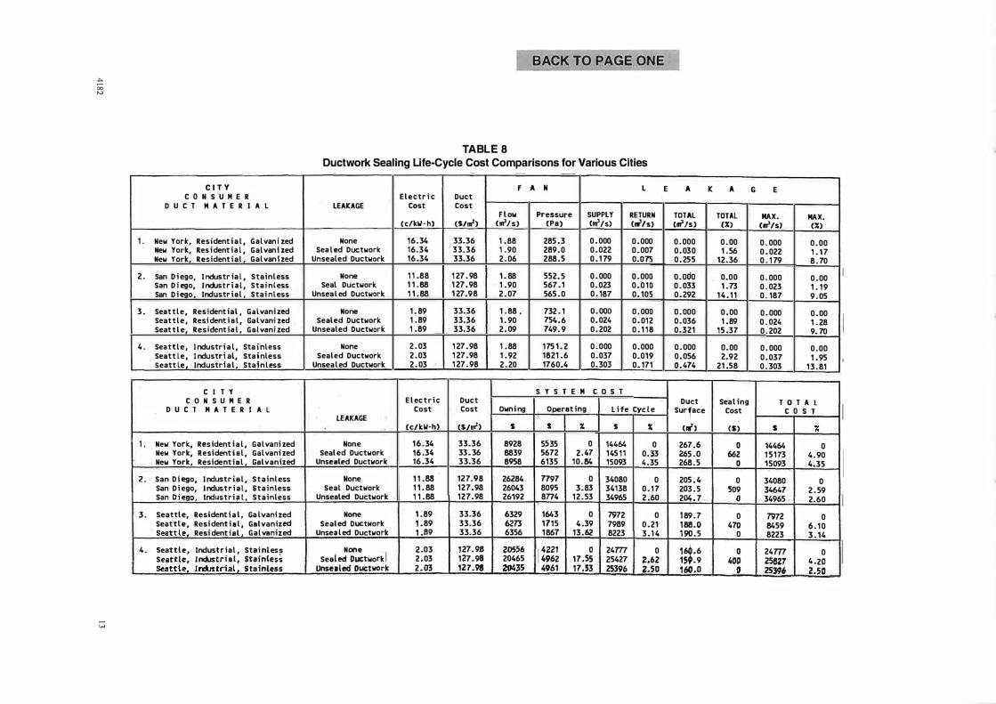
The results of the study are summarized in Table 8 where theoretical conditions at no leakage are included for compar­ison. It was found that higher system leakage increased both operating and owning costs. Tables 9 through 1 2 present the results of the parametric study. Figure 5 is a graphical repre­sentation of the results. There is a small range where duct sealing is not recommended: operating cost multiplier (OCM) is less than 2 (which is mostly exhaust systems), electricity cost is less than 2.00¢/k.Wh, and sealing cost is higher than $1 .501m2.

CONCLUSIONS

Methodology was developed to add duct leakage to the T-method previously developed for the design and simula­tion of systems. It is shown that in most cases the sealing of ductwork is economical. Duct sealing is not recommended

Telephone conversation with J. H. Stratton, director of technical services. SMACNA, Chantilly, Va., March 21 , 1990.

t Telephone conversation with Mr. C. R. James, vice president, the Robert Irsay Company, Skokie, Ill., November 28, 1 990.

4 182

BACK TO PAGE ONE

when the operating cost multiplier (OCM) is less than 2 (generally exhaust systems), electricity cost is less than 2.00¢/k.Wh, and sealing cost is greater than $ 1 .501m2. A simple rule is: the higher the system cost, the greater the need for ductwork sealing.

ACKNOWLEDG MENT

The work reported in this paper is the result of cooperative research between the American Society of Heating, Refriger­ating and Air-Conditioning Engineers, Inc. (ASHRAE), and NETSAL & Associates.

NOMENCLATURE

A

As

c

== duct cross-sectional area, m2 (ft2)

== duct surface, m2 (ft2)

== local loss coefficient, dimensionless

== leakage class, dimensionless

== duct diameter, m (in.)

== equivalent-by-friction diameter of rectangular duct, m (in.)

== equivalent-by-velocity diameter of a rectangular

E

Eb

Ee

Ep

Es

f H

L

LCC

M

OCM

Sd

Ss

duct, m (in.)

== present worth owning and operating cost, $

== basic operating cost, $

== electrical energy cost, $/kWh

== operating cost, $

== owning cost, $

== friction factor, dimensionless

== duct height, m (in.)

== duct length, m (in.)

== life-cycle cost, $

== fan motor power, kW (hp)

== operating cost multiplier, dimensionless

== downstream pressure, Pa (in. wg)

== fan total pressure, Pa (in. wg)

== average static pressure, Pa (in. wg)

== system total pressure, Pa (in. wg)

== upstream pressure, Pa (in. wg)

== present worth escalation factor, dimensionless

== airflow, m3 Is ( cfrn)

== downstream flow rate, m31s (cfrn)

== fan flow rate, m3 Is ( cfrn)

== upstream flow rate, m31s (cfrn)

== terminal airflow with zero leakage, m31s (cfm)

== absolute roughness factor, m (ft) == duct cost, $1m2 ($1ft2)

== sealing cost, $1m2 ($1ft2)

== air temperature, "C (°F)

V == mean air velocity, mis (fpm)

I I

= average air velocity, mis (fpm)

= duct width, m (in.)

dP, Ill' = total pressure loss, Pa (in. wg)

dPp, Mp = path pressure loss, Pa (in. wg)

dPex = excess path pressure loss, Pa (in. wg)

dQ,t:.Q = flow leakage rate, m3/s (cfm)

p = air density, kg/m3 (lbm/ft3)

v = kinematic viscosity, m2/s (ft2/s)

TERMINOLOGY

The following terminology is adapted from Horowitz and Sahni (1976). References are to the system illustrated by Figure 3.

Children and parent. Duct sections connected at the same node. The parent section is the one that collects or distributes the total flow. The rest are children sections. In Figure 3, Section 3 is the parent with two children, Sections 1 and 2. Parent Section 5 has two children, Sections 3 and 4.

Path. A set of descendants connected in series. Paths from node 3-4-5 are 4, 1-3, and 2-3. Paths from the root node 5 are 1-3-5, 2-3-5, and 4-5 .

Tee. Sections linked at the same node. The tee 1 -2-3 consists of Sections 1 , 2, and 3 .

Terminal sections (nodes). Sections connected to the termi­nals : Sections 1 , 2, and 4.

12

BACK TO PAGE ONE

Tree. A system of duct sections connected at nodes with no circuits.

REFERENCES

AABC. 1983. Duct leakage and air balancing. Technical Publication No. 2-83. Washington, DC: Associated Air Balance Council.

ASHRAE. 1993. 1993 ASHRAE Handbook-Fundamentals, Chapter 32, "Duct design." Atlanta: American Society of Heating, Refrigerating and Air-Conditioning Engi­neers, Inc.

ASHRAE. 1985. ASHRAE Handbook-1985 Fundamentals (l-P edition), Chapter 33, "Duct design." Atlanta: Amer­ican Society of Heating, Refrigerating and Air-Condi­tioning Engineers, Inc.

Horowitz, E., and S. Sahni. 1976. Fundamentals of data structures. New York: Computer Science Press.

Tsai, R.J., H.F. Behls, and R. Mangel. 1988a. T-method duct design, Part I: Optimization theory. ASHRAE Transac­tions 94 (2).

Tsal, R.J., H.F. Behls, and R. Mangel. 1988b. T-method duct design, Part II: Calculation procedure and economic analysis. ASHRAE Transactions 94 (2).

Tsal, R.J., H.F. Behls, and R. Mangel. 1990. T-method duct design, Part III: Simulation. ASH RAE Transactions 96 (2).

Tsal, R.J., H.F. Behls, and L.P. Varvak. 1998. T-method duct design, Part IV: Duct leakage theory. ASHRAE Transac-

4182

� 00 "'

-!.;.)

1 .

2 .

3 .

4 .

1 .

2 .

3 .

4.

C I T Y C 0 N S U M E R

D U C T M A T E R I A L

New Yorlc, Resident i a l , Galvan zed New York, Res ident ia l , Galvan zed New York, Resident i a l Galvan zed

San D i ego, I ndustr ia l , Stainless San D i ego, I ndustri a l , Stainless San D i ego Industr i a l , Stai nless

Seat t l e , Resident ial , Galvani zed Seat t l e , Resi dent i a l , Ga lvani zed Seat t l e, Resident ia l , Galvani zed

Seat t l e , l ndustr a l , Sta nless Seatt l e , l ndustr al, Sta nless Seatt Le lndustr a l , Sta n l ess

C I T Y C 0 N S U M E R

D U C T M A T E R I A L

New York, Res ident i a l , Galvani zed New York, Resident i a l , Galvani zed New York, Resident i a l Galvanized

San D i ego, I ndustr i a l , Stainless San Di ego, I ndust r i a l , Stain less San D i ego, Industri a l , Stainless

Seattle, Resident i a l , Ga lvani zed Seattte, Resi dent i a l , Galvanized Seattle. Resi dent ial G a l vanized

Seattle, Industrial , Stai nles � Seattle, Industrial , Stainless Seattle. Industrial. Stainless

BACK TO PAGE ONE

TABLE 8 Ductwork Sealing Life- Cycle Cost Comparisons for Various Cities

-

Electr i c Duct LEAKAGE Cost Cost

Cc/kll·h) <Stm2> None 16.34 33.36

Sea l ed Ductwork 16.34 33.36 Unsealed Ductwork 16 .34 33.36

None 1 1 .88 1 27 . 98 Seal Ductwork 1 1 . 88 1 27 . 98

Unsea l ed Ductwork 1 1 . 88 1 27.98

None 1 . 89 33.36 Sealed Ductwork 1 . 89 33.36

Unsealed Ductwork 1 .89 33.36

None 2 . 03 1 27 . 98 Sealed Ductwork 2 . 03 1 27.98

Unsea l ed Ductwork 2 . 03 1 27 . 98

E l ec t r i c Duct Cost Cost

LEAKAGE Cc/kll·h> ($/of)

None 16.34 33.36 Sealed Ductwork 16 .34 33 . 36

Unsealed Ductwork 16 .34 33.36

None 1 1 .88 127.98 Seal Ductwork 1 1 . 88 127.98

Unseated Ductwork 1 1 . 88 127.98

None 1 . 89 33.36 Sealed Ductwork 1 ,89 33.36

Unsea t ed Ductwork 1 .89 33.36

None 2.03 1.27. 98 Sealed Ductwork I 2 . 03 127.98

Unse1led D1,1Ctwork 2 . 03 127.98

-

F

F l ow Cm' ts>

1 .88 1 .90 2 . 06

1 . 88 1 . 90 2 . 07

1 . 88 . 1 . 90 2 . 09

1 . 88 1 . 92 2 . 20

Owni ng

s 8928 8839 8958

26284 26043 26192

6329 6273 6356

205:16 20465 20435

A N

Pressure (Pa)

285 .3 289 . 0 288 . 5

552. 5 567 . 1 565 . 0

732 . 1 754 . 6 749. 9

175 1 . 2 1821 .6

. 1760.4

S Y S T E M

SUPPLY Cni'/s) 0 . 000 0 . 022 0 . 1 79

0 . 000 0 . 023 0 . 187

o.ooo 0 . 024 0 . 202

0 . 000 0 . 037 0.303

C O S T

L

RETURN err ts> 0 . 000 0.007 0.075

0 . 000 0 . 0 1 0 0 . 105

0 . 000 0 . 012 0 . 1 1 8

0 . 000 0.019 0. 171

Operat ing L i fe Cyc l e I

s " s " 55.35 0 14464 0 5672 2 . 47 145 1 1 0.33 6135 1 0 . 84 15093 4.35

7797 0 34080 0 8095 3.83 341.38 0 . 1 7 8n4 12.53 34965 2 .60

1643 0 7972 0 1715 4 .39 7989 0 .21 1 867 13.62 8223 3 . 1 4

1 4221 0 24m 0 4962 17.55 25427 2.62 4961 17.53 25396 z.so

E A K A G E

TOTAL TOTAL MAX. MAX. cni'ts> (%) Cm'/s) (%) 0 . 000 0 . 00 0 . 000 0 . 00 0 . 030 1 . 56 0 . 022 1 . 1 7 0 . 255 12.36 0 . 1 79 8 . 70

o.odo 0.00 0 . 000 0 . 00 0 . 033 1 . 73 0 . 023 1 . 1 9 0 . 292 1 4 . 1 1 0 . 187 9 . 05

0 . 000 0 . 00 0 . 000 0 . 00 0 . 036 1 .89 0 . 024 1 . 28 0.321 1 5 .37 0 . 202 9. 70

0 . 000 0 . 00 0 . 000 0 . 00 0 . 056 2.92 0 . 037 1 . 95 0 .474 21 .58 0 . 303 1 3 . 81

Duct Seal ing T 0 T A L Sur�ace Cost C 0 S T

<Ill' > ($) s "

267.6 0 14464 0 265 .0 662 15173 4 . 90 268.5 0 15093 4.35

205 . 4 0 34080 0 203 . 5 509 34647 2 . 59 204. 7 0 34965 2.60

1 89 . 7 0 7972 0 188.0 47P 8459 6 . 1 0 1 90 . 5 0 8223 3 . 14

1;;.6 0 24m 0 15 . 9 4011 25827 4 .20 160.0 0 25396 2.50

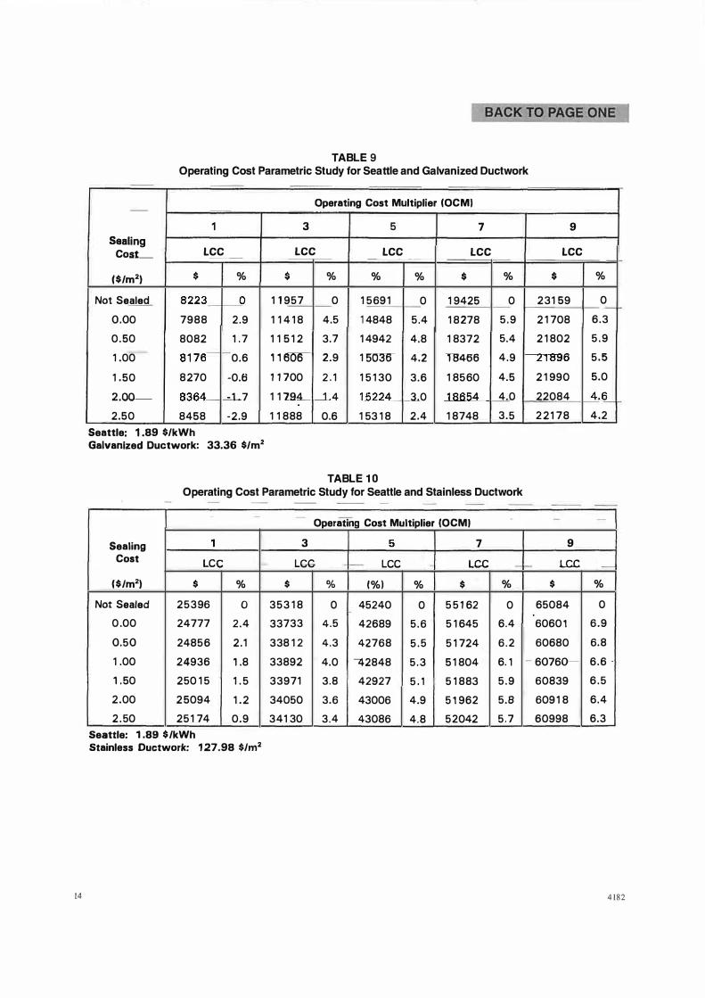
TABLE 9 Operating Cost Parametric Study for Seattle and Galvanized Ductwork

Operating Cost Multiplier fOCMJ -

1 3 5 7 9

Sealing Cost__ LCC LCC LCC LCC LCC -

($/m2) $ % $ % % % $ % $ %

Not Sealed 8223_ _o 1 1 957 0 1 5 69 1 0 1 9425 0 2 3 1 59 0 _,_ 0 .00 7988 2.9 1 1 4 1 8 4.5 1 4848 5.4 1 8 278 5 . 9 2 1 708 6 . 3

0 . 50 8082 1 . 7 1 1 5 1 2 3.7 1 4942 4.8 1 8372 5.4 2 1 802 5 . 9

1 .00 8 1 76--0.6 1 1 600 2.9 1 503lr 4.2 i"B1r66 4 . 9 21896 5 . 5

1 . 50 8 270 -0.6 1 1 700 2 . 1 1 5 1 30 3.6 1 85 60 4.5 2 1 990 5.0

2.QQ__ 8364-�7 1 1 194_ ---1.4 1 5224 __3_._0 18654 4.0 22084 4 .12...__

2.50 8458 -2.9 1 1 888 0.6 1 53 1 8 2.4 1 8748 3 . 5 2 2 1 7 8 4 . 2

Seattle: 1 .89 $/kWh Galvanized Ductwork: 33.36 $/m2

TABLE 1 0 Operating Cost Parametric Study for Seattle and Stainless Ductwork

- - -Operating Cost Multiplier (OCMJ

- - -

Sealing , 3 5 7 9

Cost LC-C - LGG LCC LCC -LCC - - -- -

f$/m2) $ % $ % {%1 % $ % $ %

Not Sealed 2 5 3 96 0 3 5 3 1 8 0 45240 0 5 5 1 62 0 65084 0

0 .00 24777 2 . 4 33733 4.5 42689 5 . 6 5 1 645 6.4 6060 1 6 . 9

0.50 2485 6 2 . 1 338 1 2 4.3 42768 5 . 5 5 1 724 6 . 2 60680 6.8

1 .00 24936 , .8 33892 4.0 �2848 5 . 3 5 1 804 6. , - 60760- 6 . 6 -

, . 50 250 1 5 1 . 5 33971 3.8 42927 5 . , 5 1 883 5 . 9 60839 6 . 5

2 .00 2 5094 1 . 2 34050 3.6 43006 4.9 5 1 962 5.6 609 1 8 6.4

2 . 50 25 1 74 0 . 9 341 30 3.4 43086 4.8 5 2042 5 . 7 60998 6.3

Seattle: 1 .89 $/kWh Stainless Ductwork: 1 27.98 $/m2

14 4182

BACK TO PAGE ONE

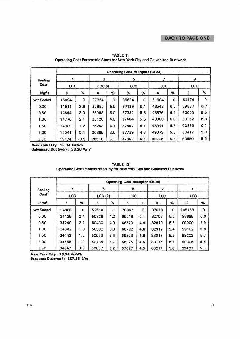
TABLE 1 1 Operating Cost Parametric Study for New York City and Galvanized Ductwork

Sealing 1

Cost LCC ($/m2.) $ %

Not Sealed 1 5094 0

0.00 1 45 1 1 3 . 9

0.50 1 4644 3.0

1 .00 1 4776 2 . 1

1 . 50 1 4909 1 . 2

2.00 1 5041 0.4

2.50 1 5 1 74 - 0 . 5

New York City: 1 6.34 $/kWh Galvanized Ductwork: 33.36 $/m2.

Operating Cost Multiplier (OCM)

3 5 7 9

LCC ($1 LCC LCC LCC

$ % % % $ % $ 27364 0 3 9634 0 5 1 904 0 641 74

25855 5.5 3 7 1 99 6 . 1 48543 6 . 5 5 9 8 8 7

25988 5 .0 37332 5 . 8 48676 6 . 2 60020

2 6 1 2 0 4. 5 37464 5 . 5 48808 6.0 60 1 52

26253 4. 1 37597 5. 1 48941 5.7 60285

26385 3 . 6 37729 4.8 49073 5 . 5 604 1 7

265 1 8 3 . 1 37862 4. 5 49206 5 . 2 60550

TABLE 1 2 Operating Cost Parametric Study for New York City and Stainless Ductwork

Sealing 1

Cost LCC

1$/m2.I $ % Not Sealed 34966 0

0.00 34 1 38 2 .4

0.50 34240 2 . 1

1 .00 34342 1 .8

1 . 50 34443 1 . 5

2.00 34545 1 .2

2.50 34647 0 . 9

New York City: 1 6.34 $/kWh Stainless Ductwork: 1 27.98 $/m2

4182

Operating Cost Multiplier (OCMI -

3 5 7 9

LCC ($) LCC LCC LCC

$ % $ % $ . % $ 525 1 4 o 70062 0 876 1 0 0 1 05 1 58

50328 4.2 665 1 8 5. 1 82708 5 . 6 .

98898

50430 4.0 66620 4.9 828 1 0 5 . 5 99000

50532 3.8 66722 4.8 8 29 1 2 5.4 9 9 1 0_2

50633 3 . 6 66823 4.6 830 1 3 5 . 2 9 9203

50735 3 . 4 66925 4 . 5 8 3 1 1 5 5 . 1 9 9305

50837 3 . 2 67027 4.3 832 1 7 5 .0 99407

-

% 0

6. 7

6 . 5

6.3

6. 1

5 . 9

5 . 6

% 0

6.0

5.9

5 . 8

5 . 7

5 . 6

5 . 5

15