TABLE OF CONTENTS 4181

AIVC 11867

MAIN GE

T-Method Duct Design: Part IV­Duct Leakage Theory

Robert J. Tsai, Ph.D. Member ASHRAE

ABSTRACT

Herman F. Behls, P.E. Fellow ASHRAE

Studies have shown that duct leakage depends on the method of duct fabrication, method of sealing, workmanship, and static pressure differential. An equation that describes leakage as a function of leakage class and static pressure is presented in the "Duct Design" chapter of the 1993 ASHRAE Handbook. This equation is used to calculate the leakage rate through a unit of duct surface for constant duct static pressure. However, the static pressure of a leaking duct does not remain constant. This process is described by a differential equation.

The magnitude of duct leakage for a straight duct depends on internal static pressure and varies uniformly along its length (assumption). Fittings in a system cause sudden changes in static pressure; therefore, duct leakage depends on fitting locations. There are two approaches for duct system leakage calculation:

Accurate-For accurate duct leakage calculations, the duct system is divided into single sections between fittings and the leakage rate and pressure loss for each section calculated by the weighing factor method.

Approximate-For most applications, duct leakage can be calculated by approximate formulas based on the average static pressure in a duct section. Leakage calculation requires dividing the system into

sections between each fitting.

This paper, the fourth in a series on T-method duct design, discusses the theory of calculating air leakage from/into a single duct to incorporate duct leakage into the optimization and simulation calculation procedures.

INTRODUCTION

The following papers have been published for the series of T-method duct design research projects:

Leo P. Varvak, Ph.D.

"Part I: Optimization Theory" (Tsai et al. 1 988a)

"Part II: Calculation Procedure and Economic Analysis" (Tsal et al. 1 988b)

"Part ill: Simulation" (Tsal et al. 1 990)

This paper, part IV, discusses the theory of calculating air leakage from/into a single duct to incorporate duct leakage into the optimization and simulation calculation procedures. Part V covers incorporation of duct leakage into the T-method calculation technique and leakage studies to determine the economics of sealing ductwork.

Studies show that HVAC air duct systems are one of the major energy consumers in industrial and commercial build­ings. From electric energy audits, supply, return, and exhaust fans consume 25% to 50% of the energy required to operate high-rise residential and commercial buildings (ASHRAE 1 993a). Inefficient design of a duct system means that either energy is being wasted and/or excessive ductwork material is being installed. Duct system optimization offers the opportu­nity to realize significant owning and energy savings. The T-method was developed as a practical duct optimization procedure. Life-cycle cost was selected as the obj ective func­tion. The T-method duct design consists of three steps performed in a series: system condensing, fan selection, and system expansion. The papers "T-Method Duct Design, Part I and Part II'' present the theory of the method, step-by-step calculation procedures, economic analysis, and examples (Ts al et al. 1 988a, 1 988b ). Part III (Tsai et al. 1 990) discusses the simulation of existing systems. Economic analysis showed that significant cost savings are obtainable. For example, if the referenced system is constructed for a residential building in New York City and the material is low-pressure galvanized duct, the economic effect on the life-cycle cost is 53 .4%. The

Robert J. Tsai is a vice president andLeo P. Varvakis a senior analyst with NETS AL and Associates, Fountain Valley, Calif. Herman F. Behls is president of Behls and Associates, Arlington Height, Ill.

THIS PREPRINT IS FOR DISCUSSION PURPOSES ONLY, FOR INCLUSION IN ASHRAE TRANSACTIONS 1998, V. 104, Pt. 2. Not to be reprinted in whole or in part without written permission of the American Society of Heating, Refrigerating and Air-Conditioning Engineers, Inc., 1791 Tullis Circle, NE, Atlanta, GA 30329. Opinions, findings, conclusions, or recommendations expressed in this paper are those of the author(s) and do not necessarily reflect the views of ASH RAE. Written questions and comments regarding this paper should be received at ASH RAE no later than July 10, 1998.

lowest obtainable economic effect is 12% for commercial buildings in Seattle.

T-method simulation may be used in the solution of many HVAC problems. In addition to the following concerns that can be clarified by simulation, T-method is an excellent design tool for simulating the flow distribution within a system with various modes of operation:

Flow distribution in a variable-air-volume (VAY) system due to terminal box flow diversity.

Airflow redistribution due to HVAC system additions and/ or modifications.

System airflow analysis for partially occupied buildings.

Necessity to replace fans and/or motors when retrofitting an air distribution system.

Multiple-fan system operating condition when one or more fans shut down.

Pressure differences between adjacent confined spaces within a nuclear facility when a design basis accident (DBA) occurs (Farajian et al. 1 992).

Smoke control system performance during a fire when certain fire/smoke dampers close and others remain open.

According to Webster, leakage is "to let a fluid out or in accidentally." Air leakage from or into a duct system means that a part of the air will be lost and the duct system will not be able to attain design conditions. The Associated Air Balance Council (AABC 1 983) states that

in the real world, Total S ystem Balance Agencies have

measured leakage values of from 30% to 45% in some

extensive rectangular duct supply systems, and regularly

experience duct leakage rates of20% of the total quantity

supplied by the fan. The effect of air leakage in duct

systems has become a major factor in the performance of

air distribution systems.

There are many concerns associated with air leakage:

Potentially inadequate cooling (inadequate zone/room air supply).

Additional cost of fan power due to increased airflow.

Oversized fans, filters, coils, chillers, and power supply systems.

Impossibility to maintain proper pressure relationship between zones/rooms and the ambient atmosphere.

The following analysis explains the practical procedure of calculating duct leakage as a part of the T-method. Ordinary numerical methods for solving differential equations were turned down due to their inability to be combined with the T-method.

2

BACK TO PAGE ONE

LEAKAGE IN A SINGLE DUCT

Duct Leakage Formulas

Research shows that leakage in an assembled duct can be estimated by an exponential equation. According to ASHRAE (1993b) the exponent is 0.65 for turbulent flow.

(1)

where

PS

= coefficient, 1 .00 for SI units, (0.14 x 10-5 for IP units),

= average static pressure in duct section, Pa (in. WG).

The constant Cv leakage class, in this equation reflects the quality of duct construction and sealing method. It is based on experimental data and exists in the range from zero for welded duels to 1 10 for rectangular unsealed ducts. The average leakage class CL for rectangular unsealed ducts is 48 cfm/100 ft2

(ASHRAE 1 993b ). The slope n is related to the type of flow. For laminar type leakage, the flow coefficient n is 1 . The n coeffi­cient for turbulent flow leakage is in the range between 0.5 and 1 . It is recommended that n be 0.65 (ASHRAE 1 993b ).

AQ _ c 0.65 '-' - al L (2)

For typical duct construction and the method of sealing, Equation 2 is not significantly different in either the negative or positive pressure modes. Equation 2 can be used to calculate the leakage at any system point for a known internal static pressure. However, internal static pressure is constantly changing from the static pressure at the fan to the terminal inlets/outlets due to friction, dynamic losses (fittings), and leakage. It is unknown, prior to the pressure loss calculation, what the static pressure is at each duct section. Because pres­sure loss is a function of leakage, Equation 2 is not usable for practical calculations. The solution requires development and integration of a differential air leakage equation.

Air Distribution Along a Duct

The Darcy-Weisbach equations for round and rectangular ductwork are as follows:

Round:

(3a)

Rectangular:

(3b)

where the equivalent-by-friction diameter (hydraulic diame­ter) is

(4)

41 81

By using the continuity equation (V = QIA) and the aspect ratio for rectangular ducts (r = HIW), the following equations result.

or

For round ducts:

For rectangular Clucts:

v = _Q_ HW

(5a)

(5 b)

(5c)

Duct width (W) can be interpreted in terms of an equiva­lent-by-velocity diameter by equating Equations 5a and 5c and solving for W,· thus,

(7t )0.5 W = 0.5 �Dv . (6)

Equations 5a and 5 b yield the equivalent-by-velocity diameter for rectangular ducts CDv) .

(7)

Introduce the coefficientµ for round and rectangular duct systems as follows:

Round duct:

µ =/ + 'LCDIL (8a)

Rectangular duct:

(8b)

BACK TO PAGE ONE

Then substitute µ into the Darcy-Weisbach equation (Equations 3a and 3 b) using Equation 5a to obtain the follow­ing single-duct pressure loss equations for round ductwork of L=l m (ft),

-1 2 -5 /'J.P = 0.8105gc µpQ D ,

and rectangular ductwork,

-1 2 -5 /'J.P = 0.8105gc µpQ Dv .

(9a)

(9b)

Assuming that 'LC=O in Equations 8a and 8 b, Equations 9a and 9b can be replaced by Equation 10 for a straight duct of L=l m(ft).

where

-1 -5 CJ = 0.8105gc µpD

(10)

(11)

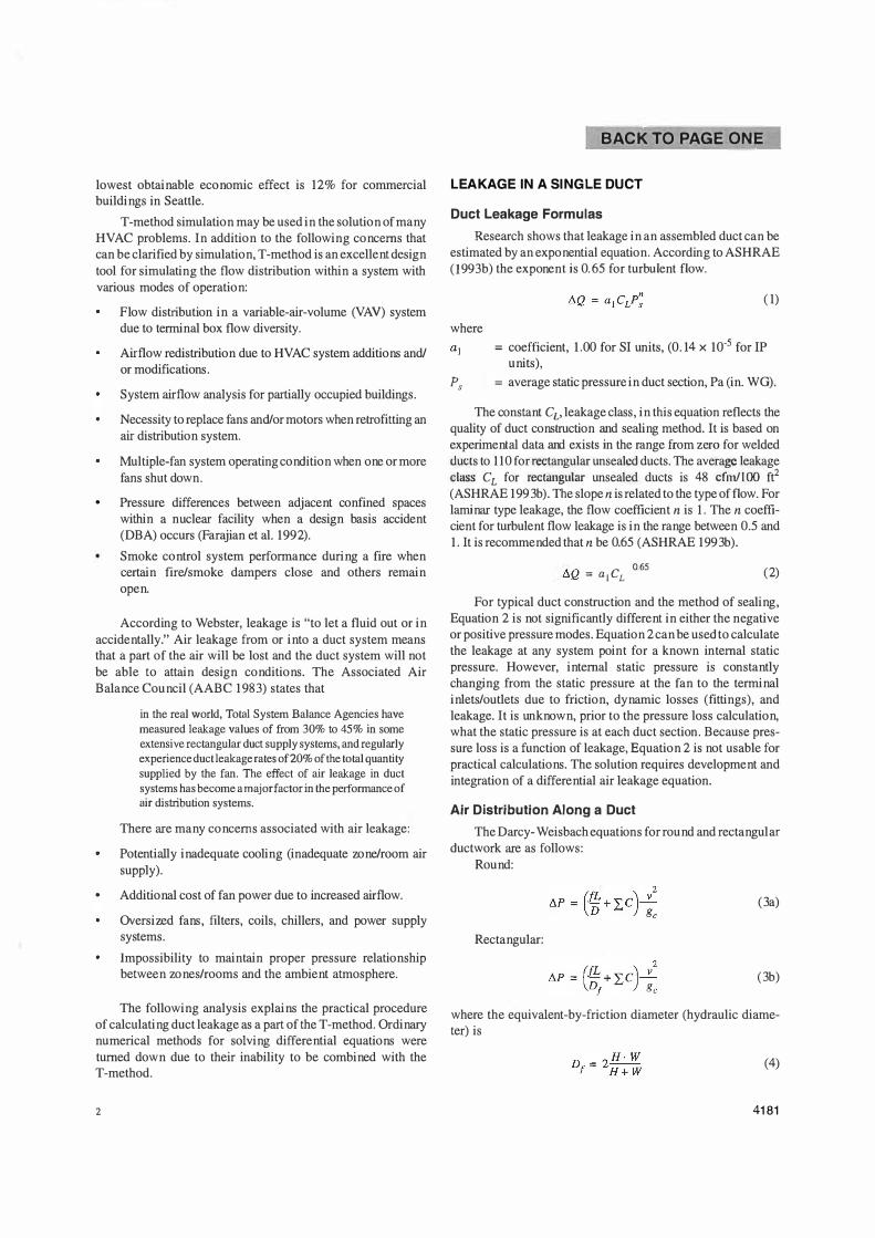
For simplification reasons, leakage ti.Q is assumed to be distributed equally over the duct length, as noted in Figure 1 . Flow upstream of the supply duct is

(12)

An approach that calculates variable flow in a duct was proposed by Konstantinov (1 981 ). Assume, on the section with the elementary length dx, that the initial flow is increasing or decreasing from Q1 to Q2 (ti.Q) and that the air velocity is changing from V1 to V2 (ti. V). The change of momentum for leaked air projected on the duct axis is

till= a0p (Q + dQ) (V + dV) - a0pQV

=a0p (Q dV + V dQ + dQ dV) (13 )

where a 0 i s the coefficient of momentum. After the low value of (dQ dV) is eliminated, the change of momentum becomes

1 2 LEAKAGE

J-J-J-J-J-J-J-J---1-J-J-!-J-J-l-J

Figure 1 Elemental duct section.

4181

-- %

3

DM = UoP (Q dV + V dQ). (14)

As shown in Figure l, the impulse of pressure forces at cross-section 1-1 and cross-section 2-2 is

IMP= PSS - (PS + dP)S = -dP s (15)

where dP = change of pressures between cross sections 1-1 and

2-2, Pa (in. wg); s = cross-sectional area, m2 (ft2).

The impulse of force for air frequency is

where X = duct perimeter, m (in);

(16)

'to = tangential stress on duct walls equal to J p g R1i, Pal m2 (in. wg/in2).

Then

IM1 = -J p g RJl(dx = -J p g S dx

where J = hydraulic slope, m (ft); Rh = hydraulic radius, m (ft).

(17)

Equate the change of momentum (D.M) to the impulse of forces due to pressure and air frequency (IMP +IM1), divide by (p g S), and assume a0=1. Then

QdV + VdQ = _dP -Jdx. Sg Sg pg But Q=(V)(S), dQ=(dV)(S), and l=dP/dx; therefore,

2 V dV + dP + dP = O . g pg

Leakage Along a Duct

(18)

(19)

Two conditions need to be considered for duct leakage: (1) initial conditions (called the Koshi problem) and (2)

boundary conditions. The Koshi problem assigns initial data for duct entry or

duct exit, such as pressure, P, and flow, Q. The results are pres­sure and flow at the other parts of a duct section. The boundary condition problem considers that pressures at both ends of a duct section are known and that airflow is the unknown. The most practical solution is the Koshi problem because for a given diameter, the flow through the duct section is unknown. Equation 19 can be written as follows (multiply by g, divide by dx) and use Equation 3 (only Darcy's part) for L=l and .EC=O:

2 2 VdV + dP = -(i)(!?J::'....) p dx dx D 2 (20)

Equation 20 can be used to develop a new duct leakage equation. Introduce the function

4

BACK TO PAGE ONE

T = Ps+p V2

and differentiate. Thus,

But

dT = !!_(P + V) = dP + d(V) . dx dx s p dx p dx

d(V) = 2 vdV

. dx dx

Substitute Equation 23 into Equation 22; then

dT = dP + 2 VdV. dx dx p dx

Equation 24 then becomes

�� = -(�)(�) ·

(21)

(22)

(23)

(24)

(25)

It i s convenient for a terminal secti on to use the length variable not from the end of the duct but from the beginning. This will change the sign of the right part of Equation 25 to plus. Let

Thus,

The leakage equation is

where k3 = 0.14 · 10-5 Cv

For round ducts, QI = (n/4) d V1

Qz = (n/4) Dz Vz As = nD L

Substitute these formulas into Equation 28; thus,

(26)

(27)

(28)

Vi -V2 = ±k P0.65

(29) L D 3 s

Substitute D. V = V2 - V1, assume L = tu, and

Then Equation 28 becomes

1W = k P0.65 6.x 2 s

When t'u¢dx and D.V¢dV, then

(31)

4181

dV = k P0.65 dx 2 s

Combining Equation 31 a with Equation 21 yields

dV . 2 o.65 dx =k2(T - pv ) .

(31a)

(32)

Finally, Equations 27 and 32, repeated below, are a system of differential equations that describes airflow in a duct with leakage.

dT = k V2 dx I

dV . 2 o.65 -=k2(T-p v ) dx

(33)

There is no analytical solution for Equation 33. An approximate numerical solution is necessary.

Let us analyze the conditions at the end of a supply duct where the air velocity is V0 and the static pressure is Ps = P0 = 0. The variable T0 at this point in the system is

(34)

The purpose of the following study is to find the variables V and T as a function of x in the range between x = 0 and x = L. The next step uses the Taylor's series for development of a linear function for static pressure Ps as a function of x.

� p =Pa + dP J x=O+ d(T-p V-)J x s dxx x = xo dx x = x0

(35 )

= dT x _ d(p v2)] x dx dx x = x0

Substitute Equation 33 into Equation 35 to obtain

PS= k, v2x-2 p v ddV J x. (36a) X X = Xo

Substitute Equation 32 into 36a; thus,

(36b)

When taking into consideration that P s = 0 at x = 0, Equa­tion 21 yields

(37)

Therefore,

(38)

Assuming that Equation 38 is valid, find solutions for T and Vin Equation 33. Substitute Equation 38 into Equation 32, taking into consideration Equation 21 . Equation 32 then becomes

41 81

BACK TO PAGE ONE

(39)

Integrating Equation 39 yields

(40)

After integration,

(41)

and

(42)

Introduce the coefficient a:

(43)

and substitute Equation 42 into Equation 33. Hence,

(44)

The integral form of Equation 44 is

(45 )

L

T1 -T0 = k1J <0a + 2 V0axt.65 + a2 x3'3)dx ( 46) 0

= k1(�L + 0.75V0aL2'65 + 0.23a2L4.3).

Considering that T0 = p 0a (Equation 34), T1 is

T1 = p Va + k1(VaL + 0.75V0aL2'65 + 0.23a2L4.3). (47)

Weighing Factor Method. Since leakage is proportional to air velocity, it would be convenient to analyze the change of air velocity instead of the change of leakage rate. Introduce the coefficients k6 and I"; thus,

(48)

(49)

Then, from Equation 42,

V1 = V0 + rxt.65. (50a)

Therefore,

�V= I"xl.65. (50b)

Considering that �Q = (V1-V2) A and x = L,

tiQ = f' L!.65 A.

Substituting Equation 50a into Equation 27 yields

Integrating Equation 5 1 yields

L

T1-T0 = k1f(l�+2V01xl.65 +r2x3·\:tx a

(50c)

(5 1 )

(52)

(53 )

(54)

Considering that T0 = p V� (Equation 34 ), T1 becomes

• 2 . 2 1.65 2 3-3 T1 = pv0+k1x(v0+0.75V0rx +0.231 x ). (55 )

The comparison between Equations 5 5 and 47 shows that they are identical. Practically speaking, leakage Q1-Q0 is smaller than 25 % of Q0• The velocity is proportional to leak­age; therefore, V1 - V0 < Vof4. From Equation 50a, Vof4 > f' xl.65. The square of both sides of this el'pression results in the following inequality: xVo/16> rx33. Therefore, the term 0.23 r2 x3·3 in Equation 55 is smaller thm1 2% of V�. Thus, Equation 55 can be simplified as

(56a)

(56b)

A new formula is developed that shows leakage as a linear combination of P s

0· 65 al the duel nodes and pressure loss as a linear combination of V2. [f the combination coefficients are defined correctly, the integral obtained will be the solution. In other words, it is necessary to find weighing average variables between duct nodes that, if used as constants, yield actual pres­sure loss and flow leakage. Following is the approl'imating formula, derived from Newton's binomial theorem, that will be used for values of"{ and any s.

(1 + "{)s = 1 + S"{ (57)

This formula is used to derive equations with respect to the coefficient a and � (linear combination) as a function of T1 , T2, V1, and V2. The linear combination derived from Equa­tion 33 follows, where dx for finite length is Land dT is tiT.

(58 )

The linear combination derived from Equation 3 1 for ti V also follows, where dx is L and dV is ti V.

6

BACK TO PAGE ONE

(59)

It is proven in the final report (Tsai and Varvak 1992) that a changes in the range between 0.5 and 0.62 (1 .65 /2.65) and that � changes in the range between 0.4 (0.65/1 .65 ) and 0.5.

The Calculation Procedure for the Weighing Factor

Method. Using previous equations, the calculation procedure for a duct with x = L length, positive pressure (supply), airflow, and velocity are known at the beginning of the duct (P 1, V1) and unknown at the end of the duct (P2, V2). First, assume P1 =0 . Then, define P0= P1 and V0 = V1• A. Case I. Terminal section, supply system.

Step 1 . Coefficient k3:

k3 = 0.14 x 10-5 CL

Step 2. Coefficient k2 (Equation 30):

kz = 4 k3/D

Step 3 . Coefficient k1 (Equation 26):

k - [2._ i- 2D

Step 4. Coefficient f' (Equation 49):

r= o.606 ki°·65 k2 vJ3

Step 5. Air velocity at L distance and velocity difference ti V (Equations 50a and 50b ):

V= Vo + r Ll.65

tiV= [' Ll.65

Step 6. Air leakage is calculated using Equation 50c:

tiQ = f' Ll.65 A

Step 7. Coefficient tiT (Equation 56b):

tiT= k1(Vo2L + 0.75 Vo f'L

2.65)

Step 8. Pressure loss (Tsai and Varvak 1992, Equation 2.9 1 ):

Static: Ms= tiT- p (V0 + tiV/2) tiV

Total: Using (),p = P s + t yields

M=tiT + 0.5 pV0tiV

where ti V and tiT are from steps 5 and 7.

B. Case II. Intermediate section. In the case of P1 > 0 the order of calculation is: Step 1 . Coefficient k3:

k3 = 0.14 x 10-5 CL

Step 2. Coefficient k2 (Equation 30):

41 81

Step 3 . Coefficient k1 (Equation 26):

k _fE._ i - 2D

Step 4. Coefficient x1 (Tsal and Varvak 1992, Equation 2.78):

Step 5 . Air velocity at L distance (Tsal and Varvak 1992, Equation 2.85) and 6 V (Equation 50b):

V _ V k VJ.3[( L)J.65 _ 1.65] 2 - I+ 6 I XI+ XI

!!..V = k6v: ·3[(x1+L{65 -x) .65]

Step 6. Air leakage is a function of air velocity; therefore:

!!..Q = k6v: .3((x1+L)J.65 -x)·65)A

Step 7. Coefficient 6T (Tsal and Varvak 1992, Equation 2.87):

!!..T = k1Lv7{1 +0.9k6v:3[(x1+L)l.65 -x) ·6

5]}

Step 8. Pressure loss (Tsal and Varvak 1992, Equation 2.9 1 )

Static: M's= 6T- p (V0 + 6V/2) 6V

Total: Using !!..P = P, + � yields

M' = 6T + 0.5 p V0!!.. V

where 6 V and !!..Tare from steps 5 and 7.

Approximate Method

It is assumed that the variableP8 in Equation 2 is the aver­age static pressure in a duct section.

(60)

Since

(6la)

(6 lb)

Assuming that dynamic pressure in Equations 6la and 6 1 b is always positive, the "up sign (-)" is for supply and the "down sign (+)" is for return/exhaust duct. Substitute Equa­tions 6la and 6lb into 60 to obtain Equation 62a.

41 81

BACK TO PAGE ONE

(62a)

For a terminal section P2 = 0 and V2 = O; therefore, Equa­tion 62a becomes

(62b)

Substitute V = QIA into Equation 62a; thus,

(63 )

Substitute Equation 63 into Equation 2 instead of M's and multiply by the duct surface area As to obtain leakage for the section.

For a terminal section where P2 = 0 and Q2 = 0,

(64b)

The average flow rate can be described as follows:

(65 )

Substituting Equation 65 into Equation 10 and solving with respect to Q1,

(66)

where

(67)

Finally, airflow at the beginning of the section is

Introducing the variable k,

k = k ' + 0.5 6Q M'--0·5, (69)

and substitute k into Equation 68. Note that Equation 69 is similar to the original T-method equation below (Tsai at el. 1990, Equation 19).

Q1 = k6P0.5 (70)

or

(Q.)2 !!..P = k (71 )

7

Leakage Evaluation

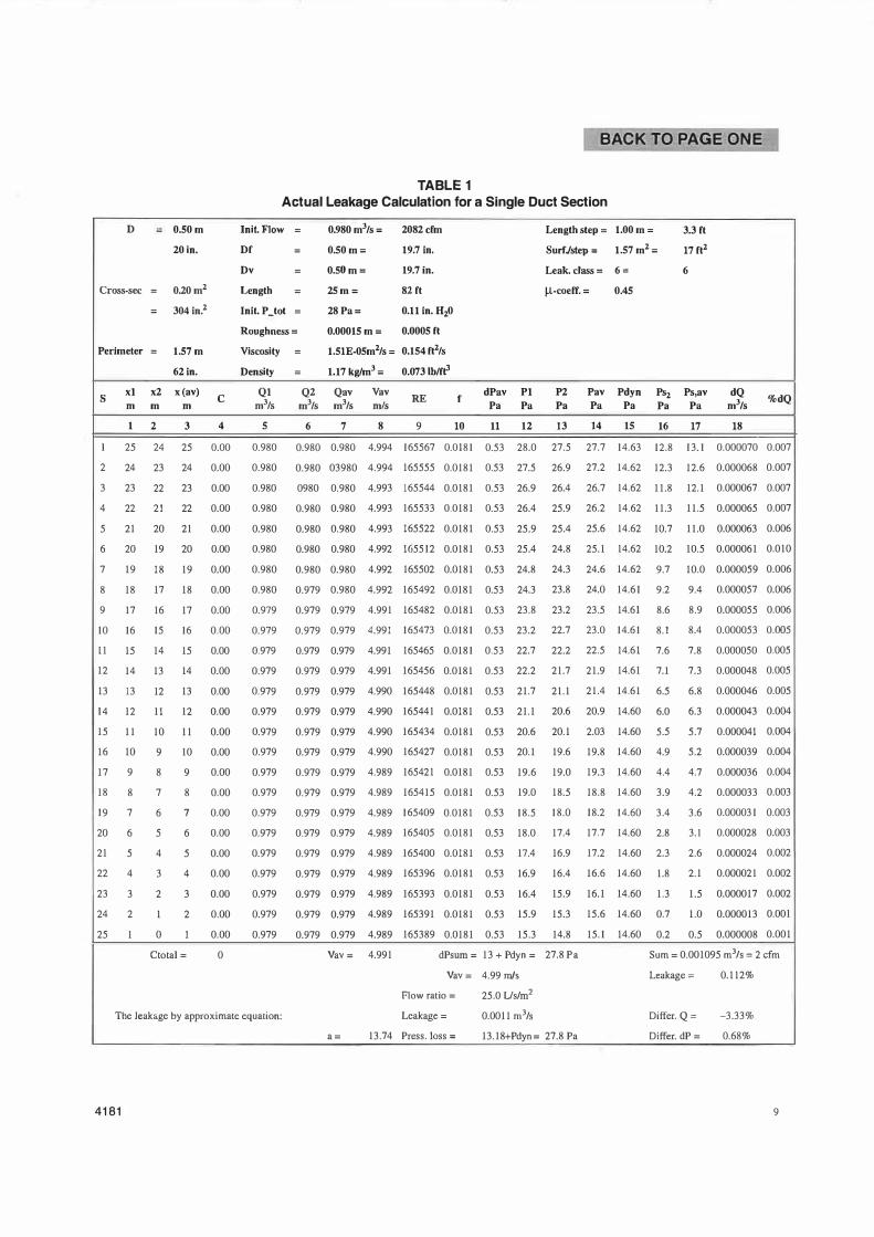
Actual and Approximate Solutions. In order to select a methodology (equation) for duct leakage calculation, a one­section duct system is analyzed for the three air leakage calcu­lation procedures: (1 ) actual leakage (25 short duct intervals), (2) approximate formula based on average static pressure (Equation 64a), and (3 ) weighing factor method. Actual solu­tion is impractical for routine duct leakage calculations; however, it is used here to analyze the accuracy of the leakage calculation methods.

Calculation of actual leakage is presented in Table l as a result of dividing the total duct length into 25 one-meter incre­ments. The following data are calculated at each step:

Flow at the beginning (Q1), end (Q2), and average (Qav).

Average air velocity based (V0v) on average flow (Qa)·

Reynolds number (Re) and friction factor (j).

Pressure loss (dPav) based on average air velocity.

Total pressure at the beginning (P1) and end (P2) of each increment and average over the entire length (Pav).

Dynamic pressure (Pdyn) based on average air velocity.

Static pressure at the end of each increment (Psi) and the average over the entire length (Ps,av).

Leakage (dQ) based on average static pressure.

Leakage percent related to the total flow in a particular section (%dQ) .

The following data are also presented in the lower part of Table 1 :

Summation C-coefficient (Ctot, col. 4) in the section.

Average air velocity in the section (Vav, col. 8).

Total pressure loss as a sum of pressure losses in the steps (dPsum, col. 13).

Total leakage calculated as a sum of leakages at each step (Sum, col. 18).

Leakage percentage

Flow/surface ratio as used in ASHRAE ( 1993b, Chapter 32, Table 6, p. 32.15 )

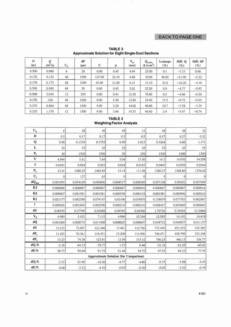
A large number of calculations based on previous proce­dures similar to the calculations presented in Table l were performed and statistical data were collected. Eight examples of using an approximate calculation for a single duct with different diameters, flows, and/or C-coefficients are presented in Table 2. The least accuracy is obtained for 40.2% leakage and C= 127.0, which is unrealistic. Even when C = 9.0 and D = 0.17 m and the pressure loss is 1500 Pa (6 in. wg) for a 25 m (82 ft) duct section, the duct leakage is 17.5% and the inaccuracy is 9.75%. It shows that when the C-coefficient is high, the approximate approach creates errors. These errors can be avoided by dividing the system into sections between each fitting (see explanation below).

8

BACK TO PAGE ONE

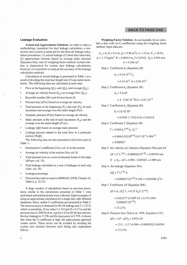
Weighing Factor Solution. As an example, let us calcu­late a duct with no C-coefficients using the weighing factor method. Input data are:

CL= 6, D = 0.5 m, Q = 0.98 m3/s, L = 25 m, P1 = 28 Pa,

p = l .17 kg/m3, R = 0.00015 m,f = 0.018 1 , Vo= 4.994 mis,

A= 0.196 m2.

Step 1 . Coefficient k3 (Equation 28):

k3 = 0. 14·10-5 CL

= 0.14·1 0-5 ·6 = 0.84·1 0-5

Step 2. Coefficient k2

(Equation 30):

kz = 4k3'D

= 4 . 0.84· I0-5/0.5 = 0.67·10-4

Step 3 . Coefficient k1 (Equation 26):

k1 =fp /(2D)

= 0.0181 ·1 . l 7 /(2·0.5) = 0.0211 8

Step 4 . Coefficient r (Equation 49):

r = o.606 k1°·65 k2 va1-3

= 0.606·0.021 18°·65 ·0.67 .1 0-4 ·4.9941.3

= 0.000027

Step 5 . Air velocity at L distance (Equation 50a) and fl V:

fl v = r L 1.65 = 0.000026· 251 ·65 = 0.00545 mis

V = V0 - fl V = 4.994 - 0.00545 = 4.989 mis

Step 6. Air leakage (Equation 50c):

flQ=r LL65 A

= 0.000027·251.65·0.196 = 0.001068 m3/s

Step 7. Coefficient flT(Equation 56b):

flT= k1CVo2 L +0.75 Vo r Ll.65)

= 0.021177 (4.9942·25 + 0.75-4.994· 0.000027. 25

1 ·65)

= 13 .2 Pa

Step 8 . Pressure loss (Tsal et al. 1992, Equation 2.9 1 )

Ms= flT- p(V0 +fl V/2) fl V

= 13 .2 - 1 . 17 (4.994 + 0.0054512) 0.00545

= l3 .2Pa

41 81

BACK TO PAGE ONE

TABLE 1 Actual Leakage Calculation for a Single Duct Section

D = 0.5 0m Init.Flow = 0.980 m3/s = 2082cfm Length step = 1.00 m = 3.3 ft

20 in. Df = 0.5 0m= 19.7 in. SurfJstep = 1.57m2= 17 ft2

Dv = 0.50m= 19.7in. Leak. class = 6= 6

Cross-sec = 0.20m2 Length = 25 m= 82ft µ-coeff. = 0. 45

= 304 in.2 Init.P_tot = 28Pa= 0.11 in. H20

Roughness= 0.00015 m = 0.0005 ft

Perimeter = 1.57m Viscosity = 1.5 1E-05m2/s = 0.15 4 ft2/s

62 in. Density = 1.17 kg/m3 = 0.073 lb/ft3

s xl x2 x(av) c Ql Q2 Qav Vav RE f dPav Pl P2 Pav Pd yn Ps

2 Ps,av dQ %dQ m m m m3/s m3/s m3/s mis Pa Pa Pa Pa Pa Pa Pa m3/s

1 2 3 4 5 6 7 8 9 1 0 11 12 13 14 15 16 17 1 8

l 25 24 25 0.00 0.980 0.980 0.980 4.994 165567 0.0181 0.53 28.0 27.5 27.7 14.63 12.8 13.1 0.000070 0.007

2 24 23 24 0.00 0.980 0.980 03980 4.994 165555 0.0181 0.53 27.5 26.9 27.2 14.62 12.3 12.6 0.000068 0.007

3 23 22 23 0.00 0.980 0980 0.980 4.993 165544 0.0181 0.53 26.9 26.4 26.7 14.62 11.8 12.1 0.000067 0.007

4 22 21 22 0.00 0.980 0.980 0.980 4.993 165533 0.0181 0.53 26.4 25.9 26.2 14.62 11.3 11.5 0.000065 0.007

5 21 20 21 0.00 0.980 0.980 0.980 4.993 165522 0.0181 0.53 25.9 25.4 25.6 14.62 10.7 11.0 0.000063 0.006

6 20 19 20 0.00 0.980 0.980 0.980 4.992 165512 0.0181 0.53 25.4 24.8 25.1 14.62 10.2 10.5 0.000061 0.010

7 19 18 19 0.00 0.980 0.980 0.980 4.992 165502 0.0181 0.53 24.8 24.3 24.6 14.62 9.7 10.0 0.000059 0.006

8 18 17 18 0.00 0.980 0.979 0.980 4.992 165492 0.0181 0.53 24.3 23.8 24.0 14.61 9.2 9.4 0.000057 0.006

9 17 16 17 0.00 0.979 0.979 0.979 4.991 165482 0.0181 0.53 23.8 23.2 23.5 14.61 8.6 8.9 0.000055 0.006

10 16 15 16 0.00 0.979 0.979 0.979 4.991 165473 0.0181 0.53 23.2 22.7 23.0 14.61 8.1 8.4 0.000053 0.005

l 1 15 14 15 0.00 0.979 0.979 0.979 4.991 165465 0.0181 0.53 22.7 22.2 22.5 14.6! 7.6 7.8 0.000050 0.005

12 14 13 14 0.00 0.979 0.979 0.979 4.991 165456 0.0181 0.53 22.2 21.7 21.9 14.61 7.1 7.3 0.000048 0.005

13 13 12 13 0.00 0.979 0.979 0.979 4.990 165448 0.0181 0.53 21.7 21.1 21.4 14.61 6.5 6.8 0.000046 0.005

14 12 11 12 0.00 0.979 0.979 0.979 4.990 165441 0.0181 0.53 21.1 20.6 20.9 14.60 6.0 6.3 0.000043 0.004

15 11 10 11 0.00 0.979 0.979 0.979 4.990 165434 0.0181 0.53 20.6 20.1 2.03 14.60 5.5 5.7 0.000041 0.004

16 10 9 10 0.00 0.979 0.979 0.979 4.990 165427 0.0181 0.53 20.1 19.6 19.8 14.60 4.9 5.2 0.000039 0.004

17 9 8 9 0.00 0.979 0.979 0.979 4.989 165421 0.0181 0.53 19.6 19.0 19.3 14.60 4.4 4.7 0.000036 0.004

18 8 7 8 0.00 0.979 0.979 0.979 4.989 165415 0.0181 0.53 19.0 18.5 18.8 14.60 3.9 4.2 0.000033 0.003

19 7 6 7 0.00 0.979 0.979 0.979 4.989 165409 0.0181 0.53 18.5 18.0 18.2 14.60 3.4 3.6 0.000031 0.003

20 6 5 6 0.00 0.979 0.979 0.979 4.989 165405 0.0181 0.53 18.0 17.4 17.7 14.60 2.8 3.l 0.000028 0.003

21 5 4 5 0.00 0.979 0.979 0.979 4.989 165400 0.0181 0.53 17.4 16.9 17.2 14.60 2.3 2.6 0.000024 0.002

22 4 3 4 0.00 0.979 0.979 0.979 4.989 165396 0.0181 0.53 16.9 16.4 16.6 14.60 1.8 2.1 0.000021 0.002

23 3 2 3 0.00 0.979 0.979 0.979 4.989 165393 0.0181 0.53 16.4 15.9 16.1 14.60 1.3 1.5 0.000017 0.002

24 2 1 2 0.00 0.979 0.979 0.979 4.989 165391 0.0181 0.53 15.9 15.3 15.6 14.60 0.7 1.0 0.000013 0.001

25 I 0 I 0.00 0.979 0.979 0.979 4.989 165389 0.0181 0.53 15.3 14.8 15.1 14.60 0.2 0.5 0.000008 0.001

Ctotal= 0 Vav= 4.991 dPsum = 13 + Pdyn = 27.8 Pa Sum= 0.001095 m3/s = 2 cfm

Vav= 4.99 mis Leakage= 0.112%

Flow ratio= 25.0 Us/m2

The leakage by approximate equation: Leakage= 0.0011 m3/s Differ. Q = -3.33%

a= 13.74 Press. loss = 13.18+Pdyn = 27.8 Pa Differ. dP = 0.68%

4181 9

D Q (m) (m3/s) CL

0.500 0.980 6

0.170 0.134 48

0.170 0.175 48

0.500 0.990 48

0.500 3.010 12

0.170 .326 48

0.270 0.860 48

0.320 1.170 12

CL 6

D 0.5

Q 0.98

L 25

pt 28

v 4.994

f 0.0181

Ps 13.41

c, 0

dQlah 0.001095

K3 0.000008

K2 0.000067

Kl 0.021177

r 0.000026

dV 0.00545

V2 4.989

dQ 0.001069

dT 13.215

dP8 13.183

dP1 13.23

dQ,% -2.36

dP,% 58.77

dQ,% -3.33

dP,% 0.68

10

BACK TO PAGE ONE

TABLE 2 Approximate Solution for Eight Single-Duct Sections

dP (pa)

28

1500

1500

28

250

1500

1500

1500

48

0.17

0.1339

25

1500

5.81

0.024

1480.25

127

0.054109

0.000067

0.001581

0.082588

0.001865

0.37799

5.432

0.008575

73.097

70.361

74.38

-84.15

95.04

-21.90

-2.22

v •• Qratlo Leakage c µ (mis) (L/s-m2) (%)

0.00 0.45 4.99 25.00

127.00 22.10 4.40 10.00

63.00 11.20 6.15 13.10

0.00 0.45 5.02 25.20

0.00 0.41 15.30 76.80

9.00 2.50 12.80 24.40

9.00 3.26 14.02 40.60

9.00 3.66 14.35 46.60

TABLE 3 Weighting Factor Analysis

48 48 12

0.17 0.5 0.5

0.1753 0.99 3.015

25 25 25

1500 28 250

7.64 5.04 15.36

0.023 0.018 0.0163

1465.85 13.14 111.98

63 0 0

0.056096 0.008517 0.008569

0.000067 0.000067 0.000016

0.001581 0.000538 0.000134

0.079147 0.02106 0.019070

0.002590 0.000216 0.000216

0.52488 0.04395 0.04386

7.115 4.996 15.316

0.011908 0.008625 0.008607

121.446 13.461 112.726

116.431 13.200 111.936

123.81 13.59 113.12

-78.77 1.27 0.44

91.75 51.46 54.75

Approximate Solution (for Comparison)

-16.20 -4.77 -4.86

-4.10 -0.93 -0.30

0.1

40.02

32.0

0.9

0.3

17.5

10.7

2.4

48

0.17

0.3264

25

1500

14.3

0.0403

1380.37

9

0.057108

0.000067

0.001581

0.138679

0.008427

1.70726

12.593

0.038732

772.445

740.471

786.23

-32.18

47.55

-9.75

-5.03

Diff. Q Diff. dP (%) (%)

-3.33 0.68

-21.90 -2.22

-16.20 -4.10

-4.77 --0.93

-4.86 --0.30

-9.75 -5.03

-7.58 -3.39

-5.47 --0.74

48 12

0.27 0.32

0.86 1.171

25 25

1500 1500

14.976 14.558

0.0359 0.0344

1368.80 1376.02

9 9

0.09202 0.027909

0.000067 0.000016

0.000996 0.000210

0.077783 0.062887

0.003869 0.000685

0.78384 0.13880

14.192 14.419

0.044857 0.011157

453.253 335.585

438.799 333.198

460.13 336.77

-51.25 -60.02

69.23 77.55

-7.58 -5.47

-3.39 -0.74

4181

M =Lff + 0.5 p V0�V

= 13 .2 + 0.5 -1 .17·4.994·0.00545

= 1 3 .2 Pa

The weighing factor solution is:

�Q (%) = (0.001 068 - 0.001 095)/0.001 095 · 1 00 = -2.36%

M (%) = (28 - 13 .2)/28 ·1 00 = 52.7 %

The results of weighing factor analysis for a number of problems are shown in Table 3. As shown in Table 3, leakage accuracy is very high for all the cases where the C-coefficients are zero. Calculations by the weighing factor method are slightly better for cases when C1 = 0 than by the approximate method. However, the weighting factor method poorly calcu­lates pressure loss.

E

i ! �

0 0019

0,0018

0.0017

0.0016

0 0015

D 001'4

0 0013

0 0012

0 0011

0 001

0 0009

a oooe 0 0007

0 0006

o.ooo:; 0 0004

0 OOO:l

0 0002

One-section Duct System

.... f-...

' .......

..., "'-

- '- ' ' '

' 25 24 23 22 21 20 1!J 18 17 16 15 1"4 13 12 11 10 9 II 7 6 5 1 J 2

Ol&t"nce, m

a Local resistance uniformly distributed.

One-section Duct System

o ao1•

0 0013

0.0012 0 0011

0"001

� o.ooo!il i !

0 0007

i 0 0005

,...,...._ ...... ,.._ ,_. ,._

O OOQ.oll ,.__ 0 OODl r-.."'-0 0002

0.0001

25 24 2 3 22 21 20 19 18 17 16 15 14 13 12 ,, 10 Iii 8 7 6 5 ..

Di&t.11nc111. m

c Local resistance at the beginning of a duct section

p...., l 2

BACK TO PAGE ONE

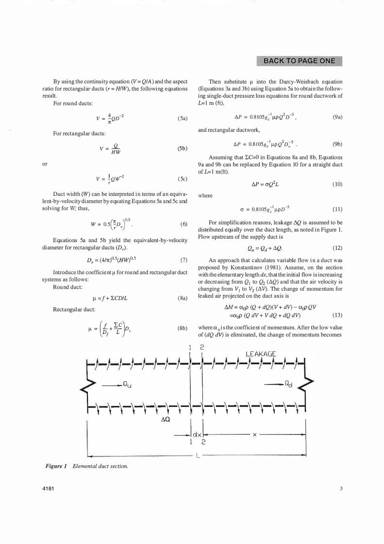
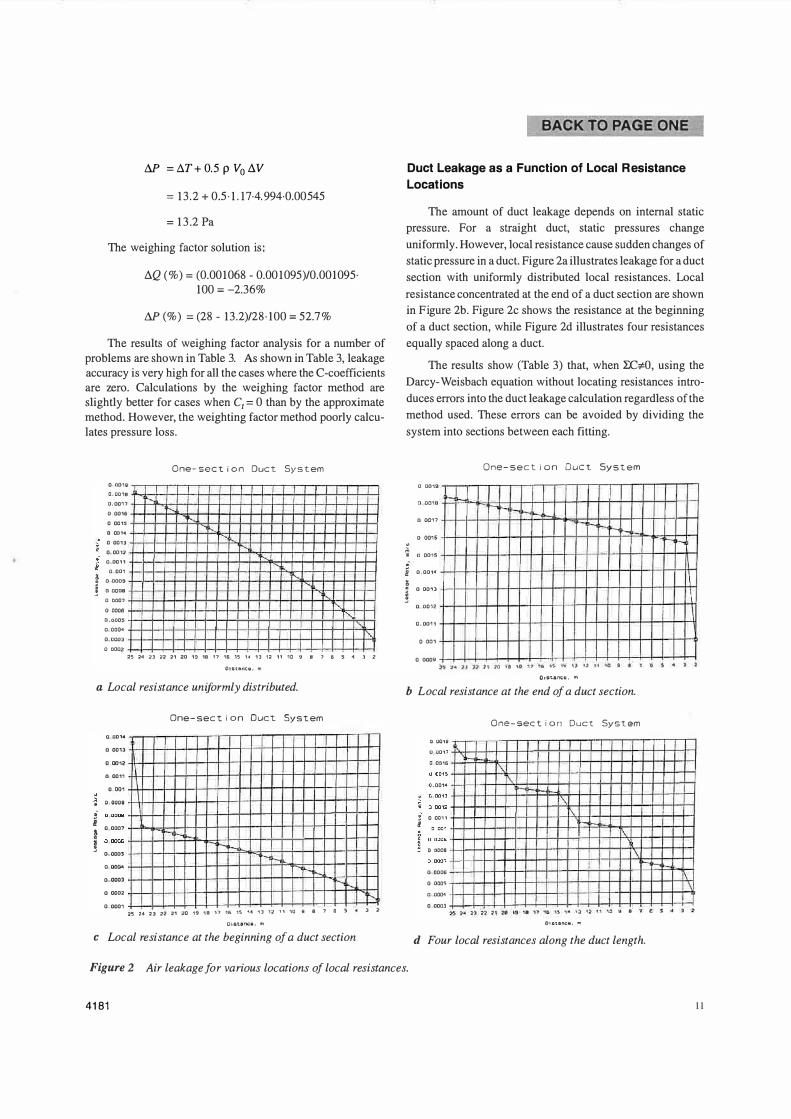
Duct Leakage as a Function of Local Resistance

Locations

The amount of duct leakage depends on internal static pressure. For a straight duct, static pressures change uniformly. However, local resistance cause sudden changes of static pressure in a duct. Figure 2a illustrates leakage for a duct section with uniformly distributed local resistances. Local resistance concentrated at the end of a duct section are shown in Figure 2b. Figure 2c shows the resistance at the beginning of a duct section, while Figure 2d illustrates four resistances equally spaced along a duct.

The results show (Table 3 ) that, when :EC;eO, using the Darcy-Weisbach equation without locating resistances intro­duces errors into the duct leakage calculation regardless of the method used. These errors can be avoided by dividing the system into sections between each fitting.

One-section Duct System

0 00151

,_ �._, ,_._ .....

0 0018

............. """'-...... a 0011

-.... 0 0016 . � o oa1s . i 0.001'1

� D 00'13

� 0 0012

a 0011

0 001

a 0009

� {14 JJ )) "11 70 1i. '\O ,, ,., t'f, 14 U '' I" !G • I I 0: S .. J 1 01srt.arn;;!il, m

b Local resistance at the end of a duct section.

One-section Duct System

o uoie ;,_ 0 001; � 0 . 0016 I'\ "

(1.00141 ---� !'\:

I\ . 0 0011 i ._� i � D DOOB \

,_ 0 0006 '\ 0 0005 ' 0 0004

0 0003

Ol1n11nci1, m

d Four local resistances along the duct length.

Figure 2 Air leakage for various locations of local resistances.

4181 11

BACK TO PAGE ONE

/ I / I / L, 1 ,'�'--*' , 1 I

0

1-5 1-4 1-3 I

,

,

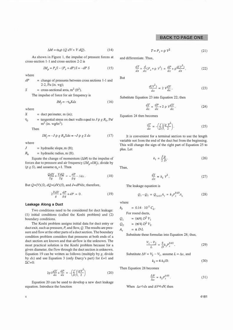
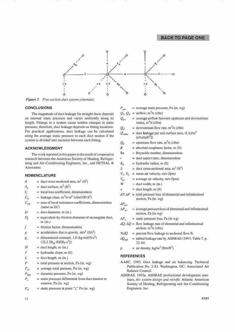
6 0 Figure 3 Five-section duct system schematic.

CONCLUSIONS

, I I I 6

The magnitude of duct leakage for straight ducts depends on internal static pressure and varies uniformly along its length. Fittings in a system cause sudden changes in static pressure; therefore, duct leakage depends on fitting locations. For practical applications, duct leakage can be calculated using the average static pressure in each duct section if the system is divided into sections between each fitting.

ACKNOWLEDGMENT

The work reported in this paper is the result of cooperative research between the American Society of Heating, Refriger­ating and Air-Conditioning Engineers, Inc., and NETSAL & Associates.

NOMENCL ATURE

f

g

H

= duct cross-sectional area, m2 (ft2) = duct surface, m2 (ft2) = local loss coefficient, dimensionless = leakage class, m3/s·m2 (cfmllOO ft2) = sum of local resistance coefficients, dimensionless

(same as LC) = duct diameter, m (in.) = equivalent-by-friction diameter of rectangular duct,

m (in.) = friction factor, dimensionless = acceleratio� due to gravity, mls2 (ft/s2) = dimensional constant, 1.0 (kg·m)/(N·s2)

(32.2 [lbm-ft]/Dbr-s2]) = duct height, m (in.)

J = hydraulic slope, m (ft) L p Pav Payn P,

12

= duct length, m (in.) = total pressure at section, Pa (in. wg) = average total pressure, Pa (in. wg) = dynamic pressure, Pa (in. wg) = static pressure differential from duct interior to

exterior, Pa (in. wg) = static pressure at point "i," Pa (in. wg)

X3 1-2 X2

"\, I

"\, I I 6

Psav = average static pressure, Pa (in. wg) Q1, Q2 = airflow, m3/s (cfrn)

= average airflow between upstream and downstream nodes m3/s (cfm)

= downstream flow rate, m3/s (cfrn) = duct leakage per unit surface area, (Us)/m2

(cfm/[s/fL2]) = upstream flow rate, m3/s (cfrn) = absolute roughness factor, m (ft)

Re = Reynolds number, dimensionless r = duct aspect ratio, dimensionless

Rh = hydraulic radius, m (ft) S = duct cross-sectional area, m2 (ft2) V1, V2 = mean air velocity, mis (fpm)

V,,v = average air velocity, mis (fpm) W = duct width, m (in.) x = duct length, m (ft) dP, M = total pressure loss of elemental and infinitesimal

section, Pa (in. wg) dP•V'

M av = average pressure loss of elemental and infinitesimal section, Pa (in. wg)

M, = static pressure loss, Pa (in.wg) dQ, llQ = flow leakage rate of elemental and infinitesimal

section, m3 Is ( cfrn) %dQ = percent flow leakage to sectional flow,% dQtab = tabled leakage rate by ASHRAE (1993 , Table 7, p.

32.16) p = air density, kg/m3 (lbmlft3)

REFERENCES

AABC. 1983. Duct leakage and air balancing. Technical Publication No. 2-83. Washington, DC: Associated Air Balance Council.

ASHRAE. 1993a. ASHRAE professional development sem­inars, Air system design and retrofit. Atlanta: American Society of Heating, Refrigerating and Air-Conditioning Engineers, Inc.

4181

ASHRAE. 1 993b. ASHRAE handbook-Fundamentals, Chapter 32. Atlanta: American Society of Heating, Refrigerating and Air-Conditioning Engineers, Inc.

ASHRAE/SMACNA!fIMA. 1985 . Investigation of Duct Leakage, ASHRAE Research Proj ect 308.

Durfee, R.L. 1972. Measurement and analysis of leakage rates from seams and joints of air handling systems. AISI Proj ect No. 120 1 -351 /SMACNA Project No. 5 -7 1 . Contractor: Versar, Inc. Springfield, VA. New York: American Iron and Steel Institute/Chantilly, VA: Sheet Metal and Air Conditioning Contractors National Asso­ciation.

Faraj ian, T., G. Grewal, and R.J. Tsal. 1992. Post-accident air leakage analysis in a nuclear facility via T-method airflow simulation. 22d DOE/NRC Nuclear Air Clean­ing and Treatment Conference, Denver, October.

Horowitz, E., and S. Sahni. 1976. Fundamentals of data structures. New York: Computer Science Press.

Konstantinov, U.M. 198 1 . Hydraulics. Kiev, USSR: Vischa Scola Publishing House.

41 81

BACK TO PAGE ONE

Swim, W.B. 1984. Analysis of duct leakage. ETL Data from ASHRAE RP-308 (prepared for TC 5 .2).

Tsal, R.J., and L.P. Varvak. 1992. Duct design using the T-method with duct leakage incorporated. ASHRAE Research Proj ect 641 -RP. Contractor: NETSAL and Associates. Atlanta: American Society of Heating, Refrigerating and Air-Conditioning Engineers, Inc.

Tsal, R.J., H.F. Behls, and R. Mangel. 1988a. T-method duct design: Part I-Optimization theory. ASHRAE Transac­tions 94(2): 90-1 1 1 .

Tsai, R.J., H.F. Behls, and R. Mangel. 1988b. T-method duct design: Part II: Calculati on procedure and economic analysis. ASHRAE Transactions 94(2): 1 12- 1 5 1 .

Tsal, R.J., H.F. Behls, and R . Mangel. 1990. T-method duct design: Part III-Simulation. ASHRAE Transactions 96(2): 3 -3 1 .

Tsal, R.J., H.F. Behls, and L.P. Varvak. 1998. T-method duct design: Part V-Duct leakage calculation technique and economics. ASHRAE Transactions 104(2).

13