E I S S T U D Y O F C O R R O S I O N P R O D U C T F I L M I N P I P E L I N E S

T. Hong, H Shi, H. Wang, M. Gopal and W. P. Jepson NSF I/U CRC, Corrosion in Multiphase Systems Center,

Institute for Corrosion and Multiphase Technology, Ohio University,

Athens, OH 45701

ABSTRACT

The properties of corrosion product film formed on carbon steel in CO2-containing saltwater under the full pipe flow are examined by A. C. impedance methods. The effect of liquid velocity on the corrosion product film is discussed in this work. It is found that, for each velocity, there is a potential above which a diffusion process occurs on the electrode, and the Warburg impedance coefficient increases with increasing potential. It is suggested that the corrosion product film formed on the surface of the steel is porous, and the diffusion process occurs through the pores of the film. By calculation of the Warburg impedance coefficient (or), the critical potential (Ef) for the formation of the corrosion film is estimated. It is observed that, below the velocity of 1.25m/s, Ef decreases with increasing flow velocity. On the contrary, at velocities above 1.25m/s, Ef increases with increasing flow velocity. It is considered that, at low velocities, the iron dissolution increases with increasing velocity, so high iron dissolution leads to high possibility for formation of corrosion product film. However, at very high velocity, i. e. above 1.25rn/s, because the shear stress at the surface of the pipeline becomes much high, the iron ions from corrosion are removed away from the metal surface, thus forming a film at the metal surface becomes difficult.

Keywords: Carbon steel, C02 corrosion, Corrosion product film, pipelines, Liquid velocity, Electrochemical Impedance Spectroscope

INTRODUCTION

The Electrochemical techniques have been widely used to examine the corrosion layer formed on steels in atmosphere environments 1-8 Some authors obtained relationships between corrosion and the

Copyright @2000 by NACE International.Requests for permission to publish this manuscript in any form, in part or in whole must be in writing to NACE International, Conferences Division, P.O. Box 218340, Houston, Texas 77218-8340. The material presented and the views expressed in this paper are solely those of the author(s) and are not necessarily endorsed by the Association. Printed in U.S.A.

corrosion layer. Grimm and Landolt 2 explained that a mass transport limited current plateau is due to the corrosion product layer formation. They pointed out that the rate of dissolution at the limited current was controlled by the rate of mass transport of ferrious ion from the layer into the solution. Hong and his co- workers 7 suggested that the growth of pitting corrosion of stainless steel depended on the thickness of the corrosion product layer. Their study indicated that the thicker the layer, the deeper the pores in the film, showing that the growth of pits on surface becomes easier.

Carbon dioxide corrosion is a great concern in oil and gas pipelines. As corrosion product layers play a very important role in carbon dioxide corrosion, many corrosion workers have focused their studies on these layers in carbon dioxide environment. 911 It has been suggested that the corrosion product layers formed on steel in carbon dioxide environment are composed of an insoluble corrosion product, iron carbonate (FeCO3), and/or undissolved component from the steel, namely cementite (Fe3C). There are two kinds of corrosion product layers. One layer is protective, and the other is unprotective. The protective layer formed on the steel surface has been suggested to be porous layer and the corrosion is inhibited by the diffusion of ions through the layer. 1°'~1 Gou et al used electrochemical methods to investigate corrosion product layer in formed diglycolamine solutions saturated with carbon dioxide at different temperatures. They found that, at 100 °C, a tight corrosion product layer was formed on the carbon steel surface and the corrosion rate become very low. They emphasized the strong inhibition of anodic dissolution due to the slow diffusion in the film.

All of the results above, however, were obtained from the Rotating Cylinder Electrode system (RCE). Little information has been reported concerning the electrochemical behavior of corrosion layers formed on steel in pipe flow. In present work, the measurements of electrochemical impedance spectrum (EIS) were carried out in pipelines under full pipe flow. The effect of liquid velocity on the corrosion product film formed on carbon steel in carbon dioxide-saturated salt water was discussed.

EXPERIMENTAL

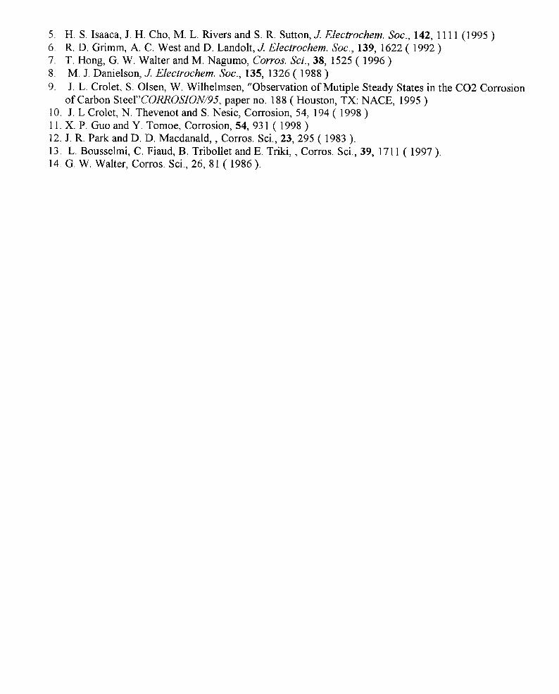
Experiments were carried out in 101.6mm I.D., 15 m long acrylic pipeline. The schematic layout of the system is given in Figure 1. Full pipe flow is a flow pattern with a single liquid phase flowing along the flow loop without feeding gas. The flow rate of the liquid phase can be controlled by a bypass line B and be measured by a calibrated orifice meter D. In this work, the liquid velocities of full pipe flow were 0.75, 1, 1.25 and 1.5 m/s.

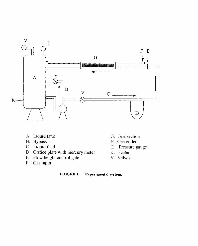
The measurements were taken in the test section as shown in Figure 2. The material was a carbon steel rod of diameter of 9mm. Before measurement, the test surface was polished with wet emery paper up to grade 600, and then cleaned by distilled water and acetone. The exposed electrode surface area was 0.71cm 2 (diameter = 9.5 mm).

All potentials recorded in this work were referred to silver-silver chloride (Ag/AgCI), and the counter electrode was an untreated stainless steel of diameter of 12.7ram

Test solution was prepared by 100% ASTM substitute saltwater. The solution was de-aerated by CO2 gas for 4 hours before testing. All experiments were performed at 40C ° with a CO2 pressure of 0.136MPa.

RESULTS AND DISCUSSION

The relationship between the corrosion product film and potential

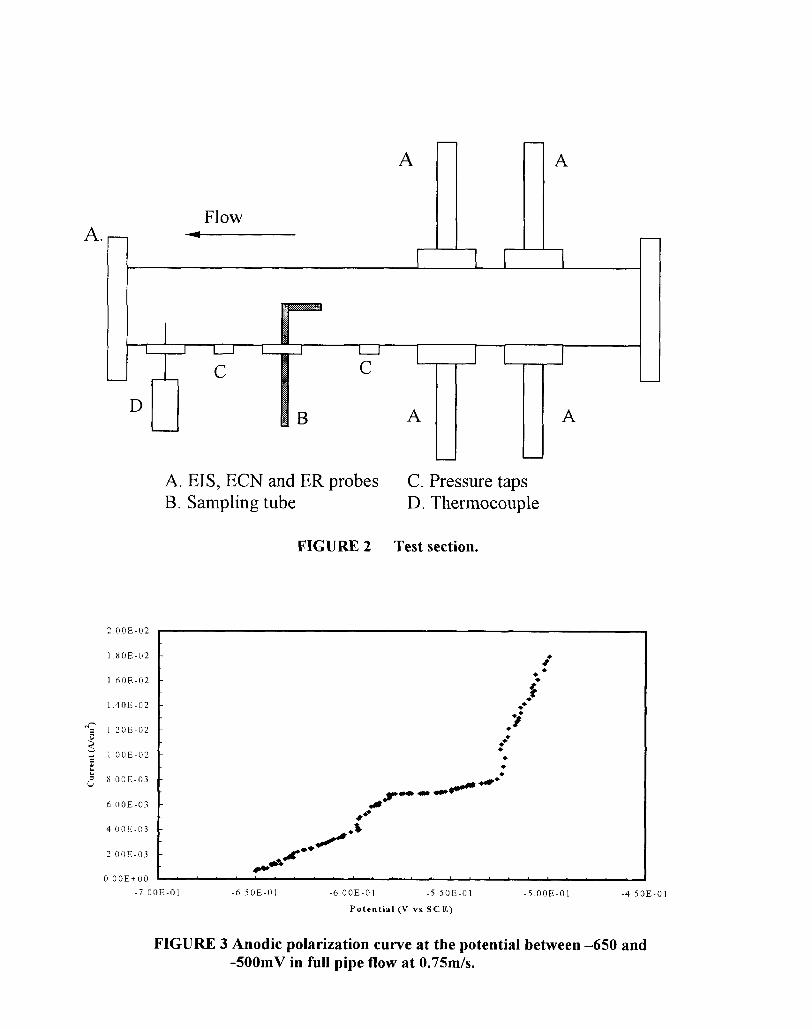
The polarization curve measured in saltwater for flail pipe flow at a velocity of 0.75m/s is shown in Figure 3. This Figure indicates that the anodic current is almost constant at the potential regions from -575 to -525mV. This means that the current is independent of the potential at the potential region between -575 to -525mV.

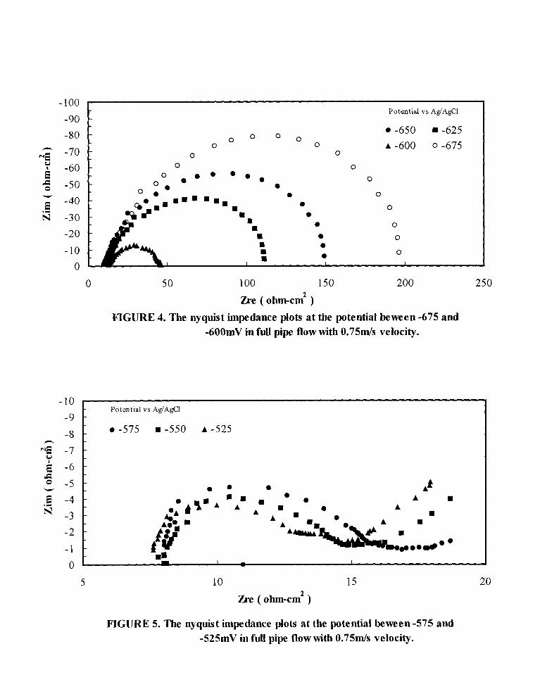
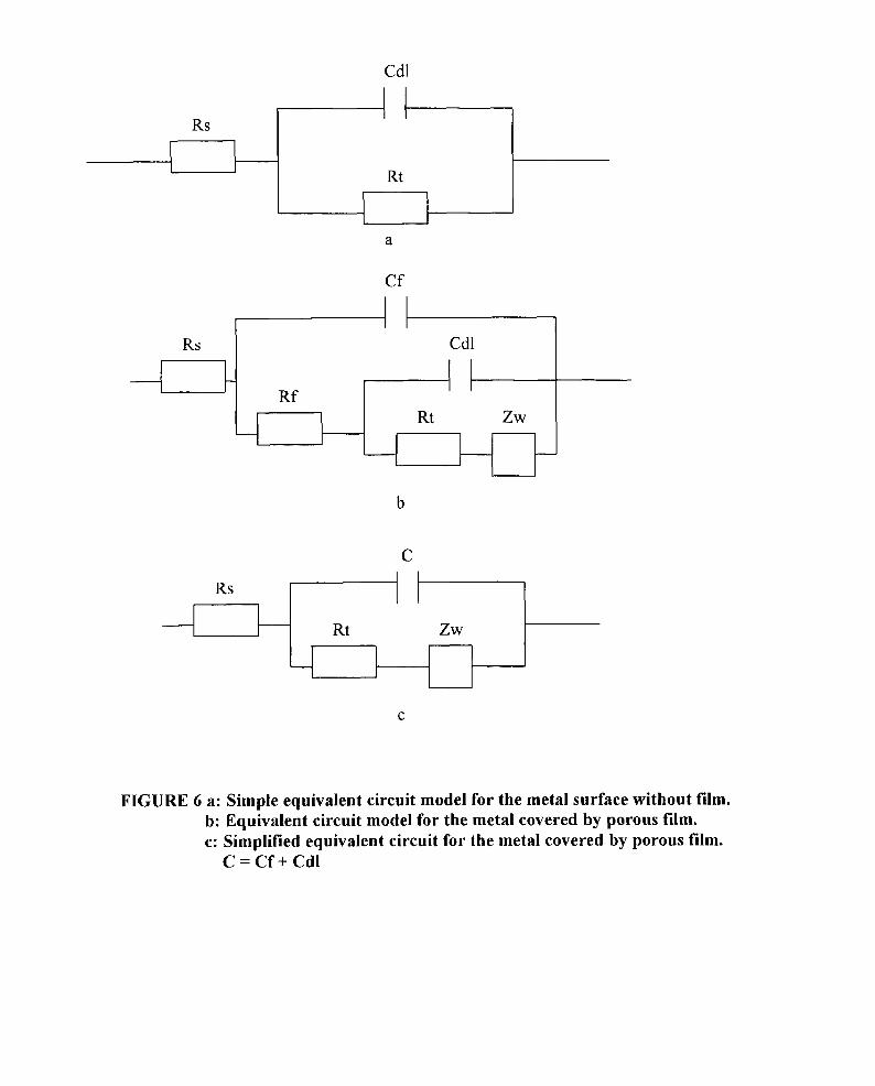
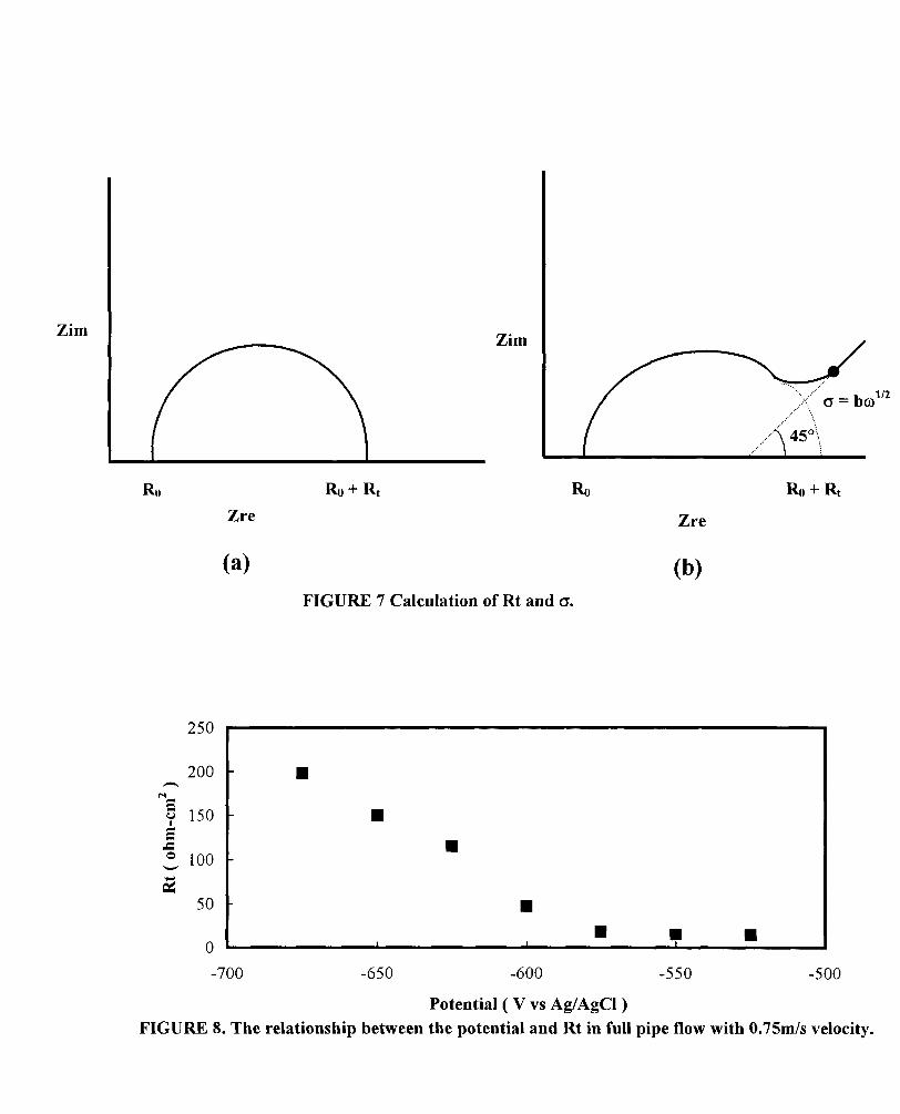
Figures 4 and 5 show the Nyquist impedance plots of the carbon steel measured at different potentials. As the potential increases from -675 (corrosion potential) to -600, Figure 4 shows that the Nyquist impedance plots are semicircles. This means that the electrode reaction is controlled by only charge transfer. This behavior can be interpreted according to a simple equivalent circuit model shown in Figure 6a. Here, R~ is the solution resistance, Rt is the metal charge-transfer resistance, and Cnf is the double layer capacitance. Rt, which represents corrosion rate, can be obtained by the intersection of the diameter of the semicircle as shown in Figure 7a. As the potential increases above -575mV, the diffusion tails appear and eventually become inclined at an angle of 45 ° to resistive axis as shown in Figure 5. In these cases, there are two reaction processes on the surface: one is metal charge-transfer and the other is diffusion. Similar impedance behavior, which consists of a diffusion tail at low frequencies, has been reported for iron and iron-chromium by other researchers. ~ They suggested that the diffiasion is due to appearance of the corrosion layer formed on the surface. Therefore, appearance of the diffusion on the electrode at the potential above -575mV indicates that the corrosion product film has formed on the surface.

There are two methods to describe the EIS spectra for the filmed or rough electrodes. One is the finite transmission line model, J2 and the other is the filmed equivalent circuit model. 13 In this work the filmed equivalent circuit model is used to describe the corrosion film covered on metal/solution interface.

The standard circuit model for filmed surface used extensively in the literature is shown in Figure 6b. 13 Here Rfand Ct, are the film resistance and capacitance, respectively, and Zw is the Warburg impedance. Zw can be presented a s 14

Zw = ~ 03 -1/2( 1-j ) (1)

Where, ~ = Warburg coefficient, Ohm-cm2-s'l/2; co = 2 rt f ( rad s "l ).

The model as shown in Figure 6b includes two parallel resistance and capacitance combinations and Warburg impedance, which are considered to contain corrosion film, metal substrate and diffusion information. 13 Two semicircles and a diffusion tail would be expected on the Nyquist plot. However, it is difficult to find two semicircles for C-1018 carbon steel exposed to the 80% saltwater-20% oil solution in Figure 5. This could result from that the high rate of wall shear stress of the turbulent flow makes the corrosion film porous. The corrosion film resistance (Rf) might be much smaller than the charge transfer resistance (Rt). The semicircle representing the corrosion film merges with the charge transfer loop. In this case, the EIS spectra for the filmed surface as shown in Figure 5 can be described by a simple equivalent circuit as shown in Figure 4c.

The warburg impedance coefficient cy can be obtained from Equation (2) by using the Nyquist impedance plots of Figure 5 at low frequencies where the diffusion tails are inclined at the angles of 45 ° to the resistive axis as shown in Figure 7b. 14

cr = bm 1/2 (2)

Where b = reactive component of impedance at which the diffusion tail begins to be inclined at an angle of 45 ° to the resistive axis, c0 = 2~xf, i.e. f: a frequency at which the diffusion tail begins to be inclined at an angle of 45 ° to the resistive axis.

Figure 8 summarizes the results of charge-transfer resistance, Rt, as a function of applied potential. At potentials above -575mV, Rt is almost constant. This means that the current density is independent of the applied potential. This behavior also can be observed by the polarization curve shown in Figure 3 on which the current is almost constant at potentials between -575 and -525mV. The ohmic drop indicates that the corrosion film is present in the surface of the steel. The largest part of the ohmic drop is across this film. Anodic dissolution in this case is inhibited by the diffusion processes through the pores in the film.

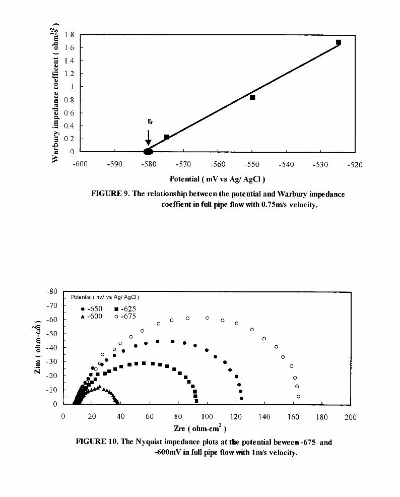
The value of Warburg impedance coefficient, o, increases with increasing the potential as shown in Figure 9. o is introduced to represent the resistance coming from the diffusion process through the pores in the corrosion layer. An increase in o indicates an increase in the resistance of diffusion process at the electrode. Since it has been suggested that the diffusion barriers on the electrode are provided by corrosion product film formed on the surface, 11 increase in diffusion barriers on the surface implies that the film becomes thicker or less porous at the more anodic potential. In another word, the corrosion film becomes more compact when the potential is increased.

The line through the points in Figure 9 intersects at the potential axis at -582 mV (Ag/AgC1). This means that the extrapolated potential for zero cy is -582 mV. Since cr represents diffusion resistance through the porous corrosion product film formed on the surface of the steel, -582 mV can be considered as the potential for zero thickness of the film. In another word, it can be suggested that -582 mV is the potential, Et; at which the corrosion film starts to grow on the surface of the steel.

The effect of liquid velocity in full pipe flow

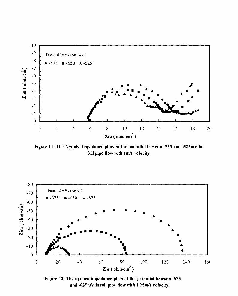
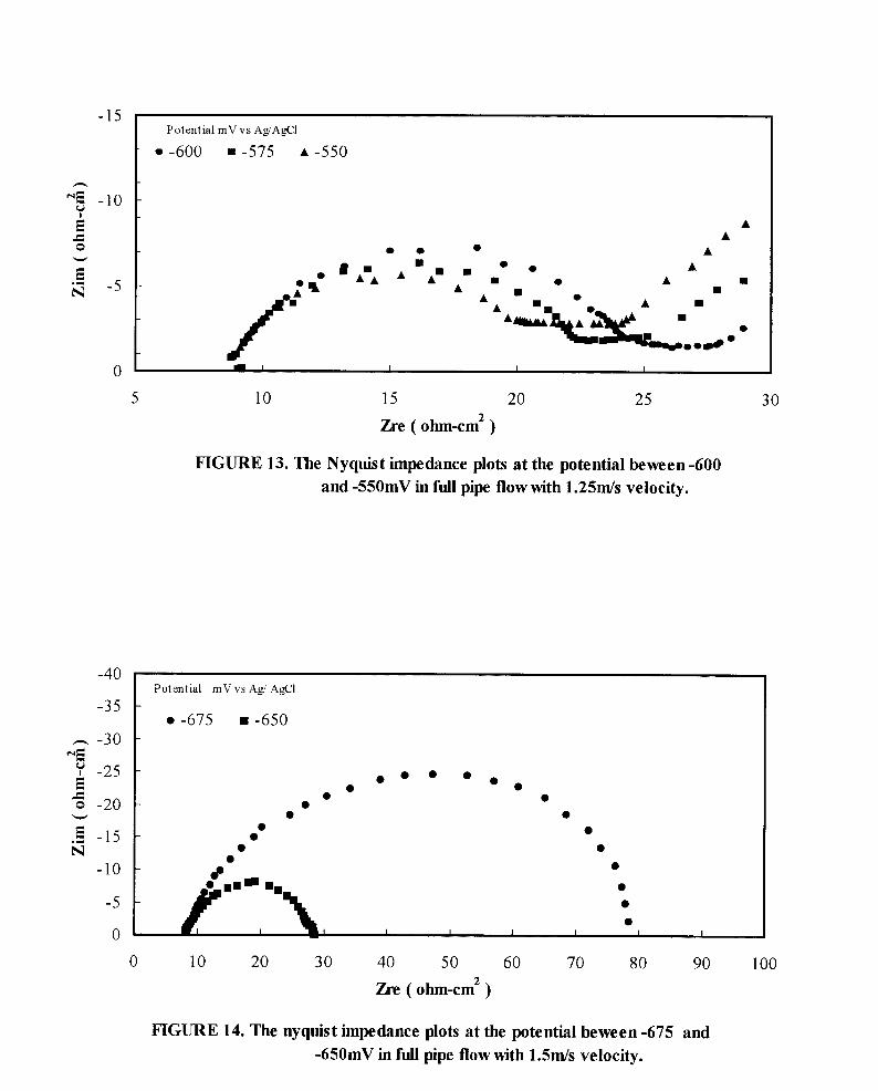
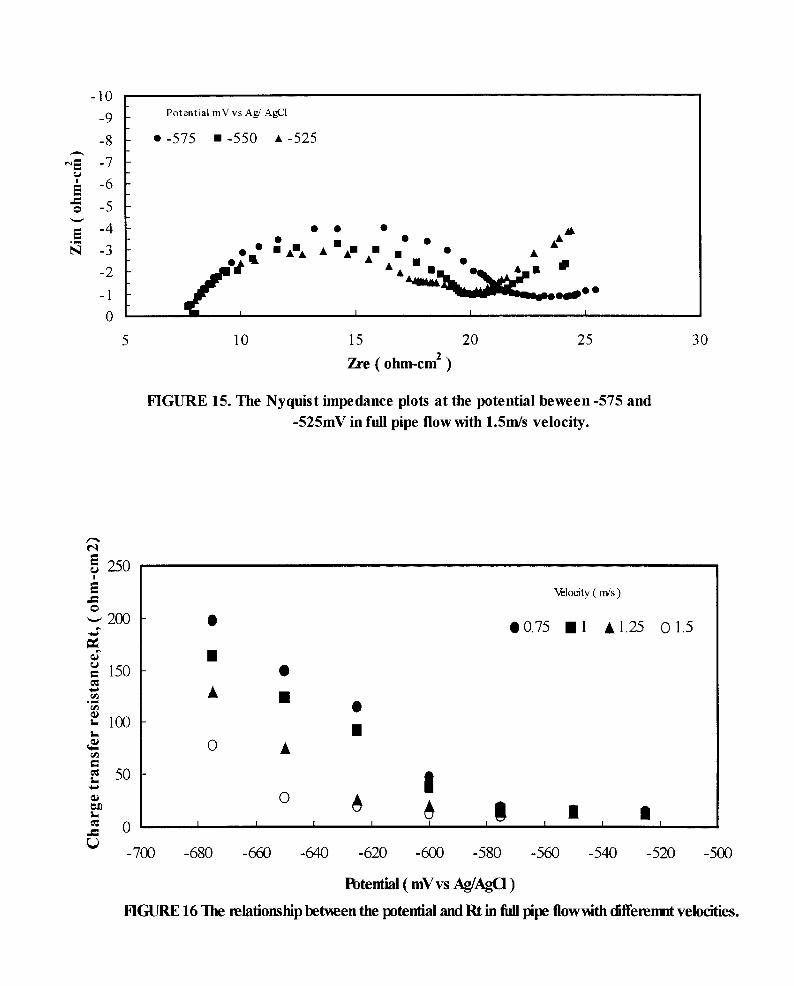
The Nyquist plots for the velocity of lrn/s at the applied potential from -675 to -600mV are shown in Figure 10. With increasing of the applied potential, the diameters of semicircles are increased. This suggests that the corrosion rate is highest at the highest potential. Figure 11 shows the Nyquist plots at applied the potential from -575 to -525mV. The diffusion process appears at this range of potential. Again, diameters of semicircles increase with the applied potential. Similar results are noted from Figures 12 to 15.

The relationship between the potential and Rt measured in different velocities is given in Figure 16. By comparison of Rt at different velocities, it is found that, at a given potential, R~ decreases with increase in velocity. This indicates that the corrosion rate becomes high as the velocity is increased. For each liquid velocity, there is a potential above which Rt is almost constant. It has been suggested that anodic dissolution is inhibited by the diffusion processes through the pores in the film.

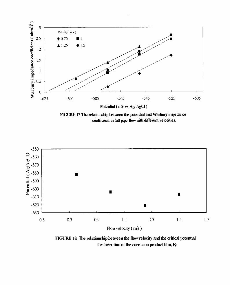
Figure 17 shows that the relationship between the potential and the Warburg diffiasion coefficient, o, with different flow velocities. It can be observed that the value of o increases with increasing the potential at a given flow velocity. Such a tendency has been suggested to occur in thicker and less porous corrosion product film at the higher anodic potential. From this Figure, it is also found that, below the velocity at 1.25m/s, o increases with increase in the velocity. An increase in cy means an increase in the diffusion barrier on the electrode. Since the diffusion barrier is provided by the corrosion product films, an increase in the diffusion barrier indicates that the film has become thicker or less porous. On the contrary, at the liquid velocities above 1.25rn/s, o decreases with increasing the flow velocity. This implies that the corrosion product film becomes thinner or more porous at the higher flow velocities. This is probably due to the shear stress at the surface of the pipeline increasing with increasing flow velocity. The high shear stress removes and damages the corrosion product film.

The lines through the points in Figure 17 intersect at the potential axis at -582, -604, -621, and - 587mV. These potentials have been suggested as the potentials, El, at which the corrosion product film starts to form on the surface of the steel. The relationship between flow velocity and Ef is given in Figure 18. It can be observed that, in the region of velocities from 0.75 to 1.5m/s, 1.25rn/s is an approximate critical velocity, below which Ef decreases and above which Ef increases with increase in velocity. This behavior can be explained by the follows: since the iron dissolution at the high velocity is higher than that at the low velocity, the higher iron dissolution leads to higher possibility for formation of corrosion product film. Therefore, Ef increases with increasing flow velocity below 1.25m/s, showing that the formation of the corrosion product film becomes easy. However, at very high velocity, i. e. above 1.251m/s, because the shear stress at the surface of the pipeline becomes much high, the iron ions from corrosion are removed away from the metal surface. In this case, forming a film at the metal surface becomes difficult, thus resulting in high Ef.

CONCLUSIONS

1. In ~11 pipe flow with the velocity of 0.75m/s, the charge-transfer resistance is almost constant when the potential is increased at the potential region between -575 and -550mV. This means that the corrosion of the steel is independent of the applied potential. Anodic dissolution in this case is inhibited by the diffusion processes through the pores in the film

2. The value of Warburg impedance coefficient, cy, increases with increasing the potential. This indicates that the protective corrosion film becomes more compact when the potential is increased.

3. Below the velocity at 1.25m/s, o increases with increase in the velocity. This implies that the corrosion film becomes thicker or less porous, showing that the film becomes compact. At the liquid velocities above 1.25m/s, c~ decreases with increasing the flow velocity. This might be because that the shear stress at the surface of the pipeline increases with increasing the flow velocity, thus remove and damage the corrosion product film, resulting in thinner or more porous corrosion film.

4. 1.25rn/s is a critical velocity, below which the critical potential for formation of corrosion film, Et; decreases and above which Ef increases with increase in velocity.

REFERENCES

1. H. C. Kou, Corros. Sci., 16, 915 ( 1976 ) 2. R.D. Grimm and D. Landolt, Corros. Sci., 36, 1847 ( 1994 ) 3. H, C Kuo and D. Landolt, Corros. Sci., 16, 915 ( 1975 ) 4. F. Hunkeler, A. Krolikowski and H. Bohni, Electrochemica Acta, 32, 615 ( 1987 )

5. H. S. Isaaca, J. H. Cho, M. L. Rivers and S. R. Sutton, J. Electrochem. Soc., 142, 1111 (1995) 6. R.D. Grimm, A. C. West and D. Landolt, J. Electrochem. Soc., 139, 1622 ( 1992 ) 7. T. Hong, G. W. Walter and M. Nagumo, Corros. Sci., 38, 1525 ( 1996 ) 8. M.J. Danielson, J. Electrochem. Sot., 135, 1326 ( 1988 ) 9. J.L. Crolet, S. Olsen, W. Wilhelmsen, "Observation of Mutiple Steady States in the CO2 Corrosion

of Carbon Steel"CORROSION~95, paper no. 188 ( Houston, TX: NACE, 1995 ) 10. J. L Crolet, N. Thevenot and S. Nesic, Corrosion, 54, 194 ( 1998 ) 11. X. P. Guo and Y. Tomoe, Corrosion, 54, 931 ( 1998 ) 12. J. R. Park and D. D. Macdanald,, Corros. Sci., 23, 295 ( 1983 ). 13. L. Bousselmi, C. Fiaud, B. Tribollet and E. Triki,, Corros. Sci., 39, 1711 ( 1997 ). 14. G. W. Walter, Corros. Sci., 26, 81 ( 1986 ).

K

V

A

/

!

)

V

G

F

V

® C

E

A. Liquid tank B. Bypass C. Liquid feed D. Orifice plate with mercury meter E. Flow height control gate F. Gas input

G. Test section H. Gas outlet I. Pressure gauge K. Heater V. Valves

FIGURE 1 Experimental system.

A. Flow

A A

D

_ _ C M C

B

A. EIS, ECN and ER probes B. Sampling tube

i I

A A

C. Pressure taps D. Thermocouple

FIGURE 2 Test section.

2 . 0 0 E - 0 2

~a

1 8 0 E - 0 2

1 6 0 E - 0 2

1 4 0 E - 0 2

1 2 0 E - 0 2

1 0 0 E - 0 2

8 0 f I E - 0 3

6 O 0 E - 0 3

4 . 0 0 E - 0 3

2 0 0 E - 0 3

0 0 0 E + 0 0

-7 0 0 E - 0 1

O

. i d

.,., .,¢°°...,.." °~ I i I I i I i I I i

-6 5 0 E - 0 1 - 6 . 0 0 E - 0 1

I i I I J I I i I I I i i

-5 5 0 E - 0 1 - 5 . 0 0 E - 0 1 - 4 . 5 0 E - 0 1

Potent ia l (V v s SCE)

FIGURE 3 Anodic polarization curve at the potential between -650 and -500mV in full pipe flow at 0.75m/s.

- 1 0 0

- 90

-80

~ -70

, -60

"~ -50

E -40

- 3 0

-20

- l O

0

P o t e n l i a l v s A ~ A g C 1

• -650 • -625 0 0 0 0

o o • -600 o -675 0 0

0 0

0 0 • • • • • 0

0 • • _ _ • • 0

i~n%ln~nnm u H i u • • • • • a O° O

• • 0

0 50 100 150 200 250

Zre (ohm-cn~)

FIGURE 4. The nyquist impedance plots at the potential beween -675 and -600mV in full pipe flow with 0.75m/s velocity.

-10

I

o ~

-9

-8

-7

-6

-5

-4

-3

-2

-1

0

P o t e n t i a l v s A g / A g C I

• -575 • -550 • -525

• • • A~

• • • A • A • • . • • • i A N • • • O A A ) i n • n m •

_ •

l q41111dmWBeee • • e O • • n i l

a m I g I

10

Zre (ohm-cm z )

15 20

FIGURE 5. The nyquist impedance plots at the potential beween -575 and -525mV in full pipe flow with 0.75m/s velocity.

Rs

Cdl

I

Rt

Cf

Ks

1 R f

Cdl

L Rt Z w

Rs

C

J Rt Zw

C

FIGURE 6 a: Simple equivalent circuit model for the metal surface without film. b: Equivalent circuit model for the metal covered by porous film. c: Simplified equivalent circuit for the metal covered by porous film.

C = C f + Cdl

Zim Zim • I ~ 0 0 1 / 2

Ro Ro+Rt Ro R o + R t

Zre Zre

(a) (b) FIGURE 7 Calculation of Rt and o.

250

e q

!

200

150

100

50

0 I I

-700 -650 -600 -550 -500

Potential ( V vs Ag/AgCI )

FIGURE 8. The relationship between the potential and Rt in full pipe flow with 0.75m/s velocity.

"• 1.8

c~ 1.6

1.4

1.2

~ 1

~ o.8

"~ 0.6

.~ 0.4

~ 0.2

~ o

-600 -590 -580 -570 -560 -550 -540 -530

Potential ( mV vs Ag/AgCI )

FIGURE 9. The relationship between the potential and Warbury impedance

coeffient in full pipe flow with 0.75m/s velocity.

-520

-80

-70

,.., -60

-50 I

-40

-30

-20

-I0

0

Potential ( mV vs A g / A g C I )

• -650 • -625 • -600 o -675 0 0 0 0

0 0 0 0

O o

0 • • • • • • 0 0 • •

0 o • • 0

~mm m mm • mmmm ° O 0 om • n m •

• • ° I t I , • o

• • 0

0 20 40 60 80 100 120 140 160 180 200

Zre ( ohm-cm 2 )

FIGURE 10. The Nyquist impedance plots at the potential beween -675 and -600mV in full pipe flow with lm/s velocity.

°I I -9 Potential ( mV vs Ag/AgCl )

-8 [- • -575 8 - 5 5 0 • -525 ] [ I - 7

? -6

i o -5 ~ • • • ~ I -4 F • ; . , . " , , " • , , I

O-- A A • • • I- lk I -3 • .m • • • I

- • • • • • • I ~ 2

-1

0

0 2 4 6 8 10 12 14 16 18 20

Zre ( ohm-cn~ )

Figure 11. The Nyquist impedance plots at the potential beween-575 and-525mV in full pipe flow with l m/s velocity.

I -70 Polential mV vs Ag/AgCI

-60 [ ° -675 " - 6 5 0 " -625 I

• . ' ' " " ' ' . I °4°~ " I 0 0 •

~o [ : . . - " " . . . " . I -20 I- e l l - • _ I

i- ~ l i t I

-10 ~ *

0

0 20 40 60 80 100 120 140 160

Zre (ohm-cm 2 )

Figure 12. The nyquist impedance plots at the potential beween -675 and -625mV in full pipe flow with 1.25m/s velocity.

-15

!

o

-10

-5

0

P o t e n t i a l m V v s A g / A g C I

• -600 • -575 • -550

• • o • •

A • mm u O • • nm •

• _ - .

"nm•m~~U,oooo o ~ •

• I I I I

5 10 15 20 25 30

Zre ( ohm-cm 2 )

FIGURE 13. The Nyquist impedance plots at the potential beween -600 and -550mV in full pipe flow with 1.25m/s velocity.

-40

-35

~ , -30

-25

-20

-15

-10

-5

0

P o t e n t i a l m V vs A g / A g C I

• -675 • -650

• • • • • • •

• O0 0 0

m 1 "pOm• m nl WHIm- • I

0 10 20 30 40 50 60 70 80 90 100

Zre ( ohm-cm 2 )

F I G U R E 14. The nyquist impedance plots at the potential beween -675 and -650mV in full pipe flow with 1.5m/s velocity.

-10

!

E

E ,ml

-9

-8

-7

-6

-5

-4

-3

-2

-1

0

P o t e n t i a l m V v s A g / A g C I

• -575 • -550 • -525

• • •

O O ~ O --mAn& I • • AI,& • • • •

I

10 15 20 25

Zre ( ohm-cn~ )

FIGURE 15. The Nyquist impedance plots at the potential beween -575 and

-525mV in full pipe flow with 1.5m/s velocity.

30

r - t

250 m

,-, 200

= 150

emil r~

100

50

0

-700

0 •

• 0.75

! o

I I I I I I I

-680 -660 -640 -620 -600 -580 -503

V e l o c i t y ( rn / s )

• 1 • 1 . 2 5 O1.5

| II I I

-540 -520 -500

Potential ( mVvs Ag/AgO )

FIGURE 16 1he relationship between the potential and Rt in full pipe flow'~ith differemnt velocities.

3

o

2.5

2

1.5

"~ 1

o.5

0

V e l o c i t y ( m / s ) 8

00.75 • 1

-625 -605 -585 -565 -545 -525

Potential ( mV vs Ag/AgO )

FIGURE 17 'Ihe relafiomhip betneen the potential and Warbmy impedance coefficient in full pipe flow~th different velocities.

I

-505

-550

< -570

< -580

.~2 -590

-600

-610

-620

-630

05

I I I I I

0.7 0.9 1.1 1.3 1.5

Flowvelocity ( nfs )

FIGURE 18. 'Ihe relationship between the flowvelocity and the critical potential

for formation of the corrosion product fdm, ~ .

1.7