t Design of a Flexure Mount for Optics in Dynamic and ... · i NASA Contractor Report 177495 Design of a Flexure Mount for Optics in Dynamic and Cryogenic Environments Lloyd Wayne

E-3

/ NASA Contractor Report 177495

Design of a Flexure Mount for Optics in Dynamic and Cryogenic Environments

t

i

Lloyd Wayne Pollard

[NBSA-CB-177495) D E S I G N OF A FLEXURE EOUMT N89-26025 FOR OPTICS EN DYNAPIIC AND CbYOGENIC ENVIBONMENTS (Arizona U n i v . ) 135 p C S C L 14B Uuclas

G 3 / 1 4 0217933

CONTRACT- NCC2-426 - February 1989

il

National Aeronautics and Space Administration

https://ntrs.nasa.gov/search.jsp?R=19890016654 2018-07-07T12:38:46+00:00Z

i

NASA Contractor Report 177495


Lloyd Wayne Pollard The University of Arizona Tucson, Arizona

Prepared for Ames Research Center CONTRACT-N CC2-426 February 1989

NASA National Aeronautics and Space Administration

Ames Research Center Moffett Field, California 94035

ACKNOWLEDGEMENTS

The author wishes to express his gratitude to the staff and faculty of the

Departments of Engineering Mechanics and Optical Sciences for the opportunity to

pursue advanced studies at the University of Arizona. In particular, a special thanks

goes to Dr. Ralph Richard for his concentrated guidance and instruction during the

past two years and for his constant availability for counsel during the last twenty

years.

Funding for this design research was provided by NASA Ames Research

Center through the NASA Cooperative Agreement NCC2-426 with the University of

Arizona. The author wishes to thank Ramsey Melugin, the technical monitor of the

NASA Ames Technical Staff, for his many contributions to this design effort and for

allowing this very interesting project to be my thesis topic.

The author wishes to acknowledge Myung Cho. m y friend and office partner

for the last two years, for his never ending patience during the many hurdles we

endured together in learning NASTRAN. And finally, a special thank you to Dorothy,

my wife. for allowing me to do this in the first place.

PRECEDING PAGE BLANK NOT FILMED

iii

TABLE OF CONTENTS

Page

a

1.

2.

3.

4.

5.

6 .

7.

8.

LIST OF ILLUSTRATIONS . . . . . . . . . . . . . . . . . . . . . . . . . . . . . . . . . . vii

LIST OF TABLES . . . . . . . . . . . . . . . . . . . . . . . . . . . . . . . . . . . . . . . . ix

ABSTRACT . . . . . . . . . . . . . . . . . . . . . . . . . . . . . . . . . . . . . . . . . . . . . INTRODUCTION . . . . . . . . . . . . . . . . . . . . . . . . . . . . . . . . . . . . . . . . .

1

2

REQUIREMENTS RESULTING FROM CRYOGENIC COOLDOWN 12 . . . . . . .

DYNAMIC ANALYSIS WITH A SINGLE DEGREE OF FREEDOM MODEL 16 Develop gimbal torsional stiffness of cruciforms. K,h. . . . . . . . . . 26 Develop gimbal torsional stiffness in flexure blades. Krs. 28 Develop flexure assembly lateral stiffnesses, hard and soft . . . . . . 30 Develop horizontal blade stiffnesses 33 Develop gimbal blade stiffnesses . . . . . . . . . . . . . . . . . . . . . . . . 35 Develop frame stiffness . . . . . . . . . . . . . . . . . . . . . . . . . . . . . . 47 Develop stability model . . . . . . . . . . . . . . . . . . . . . . . . . . . . . . 40 Finalize SDOF program . . . . . . . . . . . . . . . . . . . . . . . . . . . . . . 41 A numerical example. . . . . . . . . . . . . . . . . . . . . . . . . . . . . . . . 43 Isolated modes of the flexure blades ..................... 49

. . . . . . . ......................

DYNAMIC ANALYSIS WITH A THREE DEGREE OF FREEDOM MODEL.. 52 52 Develop the three DOF stiffness matrix ....................

Develop the eigenvalues 55 Develop the relationship between Kt and Kv. . . . . . . . . . . . . . . . 55 A numerical example.. 57

. . . . . . . . . . . . . . . . . . . . . . . . . . . . . .

. . . . . . . . . . . . . . . . . . . . . . . . . . . . . . DYNAMIC ANALYSIS WITH A NASTRAN FINITE ELEMENT MODEL . . 61

Solution Type 3 - Normal Modes Analysis . . . . . . . . . . . . . . . . 61 Solution Type 63 - Superelement Normal Modes Analysis . . . . . . 76 Solution Type 30 - Modal Frequency Response Analysis. . . . . . . 81

A COST COMPARISON OF THE SIRTF DYNAMIC ANALYSIS . . . . . . . . 84 85 85 86 87

Cost of analysis with the FORTRAN model . . . . . . . . . . . . . . . . Cost of analysis with the NASTRAN SOL 3 model. . . . . . . . . . . Cost of analysis with the NASTRAN SOL 63 model . . . . . . . . . . Cost of analysis with the NASTRAN SOL 30 model . . . . . . . . . . Cost summary of analyses . . . . . . . . . . . . . . . . . . . . . . . . . . . . 88

SUMMARY AND CONCLUSIONS . . . . . . . . . . . . . . . . . . . . . . . . . . . . . 90

REFERENCES 95 . . . . . . . . . . . . . . . . . . . . . . . . . . . . . . . . . . . . . . . . . .

V PRECEDING PAGE BLANK NOT FILMED

TABLE OF CONTENTS (continued)

Page

9. APPENDIX I Listing of FORTRAN program for SDOF parametric study . 96

10. APPENDIX I1 Listing of NASTRAN input file for SOL 3 . . . . . . . . . . . . 1 1 . APPENDIX 111 Listing of NASTRAN input file for SOL 63 . . . . . . . . . .

103

108

12. APPENDIX IV Listing of NASTRAN input file for SOL 30 . . . . . . . . . . 13. APPENDIX V Listing of NASTRAN input file for SOL 5. Buckling. . . . .

113

122

vi

LIST OF ILLUSTRATIONS

.

c

!

Figure

1.1

1.2

1.3

1.4

1.5

2.1

3.1

3.2

3.3

3.4

3.5

3.6

3.7

3.8

3.9

3.10

3.11

3.12

3.13

3.14

Page

Three Point Support Spring Model with Parallel Spring Guide ...................... 3

Parallel Spring Guide with Gimbal . . . . . . . . . . . . . . . . . . . . . . . . . . 5

Two Single Bladed Fiexure Assembly . . . . . . . . . . . . . . . . . . . . . . . . . 6

Final SDOF Design . . . . . . . . . . . . . . . . . . . . . . . . . . . . . . . . . . . . . Final Design Submitted to NASA . . . . . . . . . . . . . . . . . . . . . . . . . . . Flow Diagram for FRINGE . NASTRAN Analysis . . . . . . . . . . . . . . . Lateral SDOF Justification . . . . . . . . . . . . . . . . . . . . . . . . . . . . . . . . Reactions at Support 1 . . . . . . . . . . . . . . . . . . . . . . . . . . . . . . . . . . . Reactions at Support 2 . . . . . . . . . . . . . . . . . . . . . . . . . . . . . . . . . . . Reactions at Support 3 . . . . . . . . . . . . . . . . . . . . . . . . . . . . . . . . . . . SDOF Model . . . . . . . . . . . . . . . . . . . . . . . . . . . . . . . . . . . . . . . . . . Design PSDF Supplied by NASA Ames . . . . . . . . . . . . . . . . . . . . . . .

Gimbal Configuration . Torsion . . . . . . . . . . . . . . . . . . . . . . . . . . . . Flexure Configuration . Torsion . . . . . . . . . . . . . . . . . . . . . . . . . . . . Vertical Post Configuration . Bending and Shear . . . . . . . . . . . . . . . . . Flexure Blades Configuration . . . . . . . . . . . . . . . . . . . . . . . . . . . . . . Gimbal Blades Configuration . Axial. Shear and Bending . . . . . . . . . . . Frame Configuration . . . . . . . . . . . . . . . . . . . . . . . . . . . . . . . . . . . .

8

9

15

17

18

18

18

20

22

27

29

32

34

36

39

Free Body of Torsion Model . . . . . . . . . . . . . . . . . . . . . . . . . . . . . . . 48

Isolated Modes of Flexure Blades Model . . . . . . . . . . . . . . . . . . . . . . . 49

vii

LIST OF ILLUSTRATIONS (continued) .

Figure Page

4.1

4.2

4.3

5.1

5.2

5.3

Free Body Diagram of Three Degree of Freedom Model.. . . . . . . . . . . . Relationship Between K, and Kt . . . . . . . . . . . . . . . . . . . . . . . . . . . . Vertical Stiffness of Single Flexure Assembly. . . . . . . . . . . . . . . . . . . . NASTRAN Finite Element Model.. . . . . . . . . . . . ., . . . . . . . . . . . . . . NASTRAN Plot of Made Shape 1 - 69 Hz . . . . . . . . . . . . . . . . . . . . . NASTRAN Plot of Mode Shape 2 - 69 Hz . . . . . . . . . . . . . . . . . . . . .

54

56

58

62

63

64

5.4

5.5

5.6

5.7

5.8

NASniAN Plot of Mode Shape 3 - 73 Hz . . . . . . . . . . . . . . . . . . . . . NASTRAN Plot of Mode Shape 4 - 81 Hz . . . . . . . . . . . . . . . . . . . . . NASTRAN Plot of Mode Shape 5 - 81 Hz . . . . . . . . . . . . . . . . . . . . . NASTRAN Plot of Mode Shape 6 - 81 Hz . . . . . . . . . . . . . . . . . : . . . NASTRAN Plot of M a e Sbpe 7 - 81 Hz . . . . . . . . . . . . . . . . . . . . .

66

67

68

69

70

5.9

5.10

5.11

5.12

5.13

5.14

5.15

5.16

5.17

NASTRAN Plot of Mode Shape 8 - 81 Hz . . . . . . . . . . . . . . . . . . . . . NASTRAN Plot of Mode Shape 9 - 81 Hz . . . . . . . . . . . . . . . . . . . . . NASTRAN Plot of Mode Shape 10 - 129 Hz.. . . . . . . . . . . . . . . . . . . NASTRAN Plot of Mode Shape 11 - 129 Hz.. . . . . . . . . . . . . . . . . . . NASTRAN Plot of Mode Shape 12 - 175 Hz. . . . . . . . . . . . . . . . . . . . Modal Response Combinations . . . . . . . . . . . . . , . . . . . . . . . . . . . . . .

71

72

73

74

75

79

80

82

83

Histogram of SIRTF Natural Frequencies . . . . . . . . . . . . . . . . . . . . . . . d Typical Deflection PSD Plot From SOL 30. . . . . . . . . . . . . . . . . . . . . .

Typical Internal Load PSD Plot From SOL 30 . . . . . . . . . . . . . . . . . . .

viii

LIST OF TABLES

Table Page

2.1

4.1

5.1

6.1

7.1

Summary of FRINGE Analysis.. . . . . . . . . . . . . . . . . . . . . . . . . . . . . Element Loads for Vertical Stiffness. . . . . . . . . . . . . . . . . . . . . . . . . . First Twelve Natural Frequencies of SIRTF . . . . . . . . . . . . . . . . . . . . . Cost Comparison of the SIRTF Dynamic Analysis. . . . . . . . . . . . . . . . . Numerical Summary of Dynamic Analysis . . . . . . . . . . . . . . . . . . . . .

13

59

76

89

94

ix

.

The design of a flexure mount for a mirror operating in a cryogenic environment is

presented. This structure represents a design effort recently submitted to NASA Ames

for the support of the primary mirror of the Space Infrared Telescope Facility

(SIRTF). The support structure must passively accommodate the differential thermal

contraction between the glass mirror and the aluminum structure of the telescope

during cryogenic cooldown. Further, it must support the one meter diameter. 116

kilogram (258 pound) primary mirror during a severe launch to orbit without exceeding

the micro-yield of the material anywhere in the flexure mount. Procedures used to

establish the maximum allowable radial stiffness of the flexural mount, based on the

finite element program NASTRAN and the optical program FRINGE, are discussed.

Early design concepts were evaluated using a parametric design program, and the

development of that program is presented. Dynamic loading analyses performed with

NASTRAN are discussed. Methods of combining modal responses resulting from a

displacement response spectrum analysis are discussed. and a combination scheme

called MRSS, Modified Root of Sum of Squares, is presented. Modal combination

schemes using MRSS. SRSS. and ABS are compared to the results of a Modal

Frequency Response analysis performed with NASTRAN.

1

CHAPTER 1

INTRODUCTION

The design of the flexure mount for the primary mirror of the Space Infrared

Telescope Facility (SIRTF) is presented, and the methods used to develop that design

for NASA Ames are discussed. For the optics of SIRTF to remain unaffected by the

temperature excursions that the facility will experience in the space environment, the

optical system is cryogenically cooled with liquid helium prior to launch. This cooling

maintains the optics at a uniform temperature for operation but it also causes a

differential thermal contraction between the fused silica glass mirror'J and the

aluminum structure of the telescope due to the differences in coefficients of thermal

expansion. This contraction imposes the primary design requirement on the support

structure, which connects the mirror to its aluminum base plate. The NASA Ames

design criteria required that the support structure absorb the thermal contraction,

passively, while maintaining acceptable deflections on the mirror's optical surface and

without causing a permanent set in the qupport structure which would effect the

mirror's optical alignment. Hence, the support structure must contain a flexure mount.

A support structure that is compliant in the radial direction of the mirror

satisfies the above requirements. The launch load design criteria. on the other hand,

impose the requirement on the support structure that the three sigma working stress

during launch remains less than the micro-yield of the material. The support structure

that has the strength to satisfy that requirement is also necessarily structurally stiff.

Earlier work3 for NASA at the University of Arizona developed a three point

titanium parallel spring guide' for the flexure configuration. Shown in Figure 1.1 is a

spring model of that configuration which demonstrates the orientation of the flexure

stiffnesses as well as the orientation of the vertical parallel spring guide at each of the

2

FLEXURE ASSEMBLY < P A R A L L E L SPRING GUIDE>

T A N G E N T I A L , Kh

THREE REQUIRED A T l eg ' T Y P ONE SHOWN

r

T BASEPLATE ATTACHMENT 1

&-'PLANE OF MIRROR ATTACHMENT

Figure 1 . 1 Three Point Support - Spring Model with Parallel Spring Guide

3

three support points. A statics analysis, as will be shown in Chapter 3, demonstrates

that the net system stiffness of such a configuration is a function of the sum of the

two orthogonal stiffnesses of each flexure assembly, K, and Kh. and the net system

stiffness is independent of the assembly orientation. Therefore, the radial stiffness can

be made compliant for cryogenic cooldown and the tangential stiffness can be made

large for the launch loads. Titanium was selected as the flexure material primarily

because of its predictability under high working stress at cryogenic temperatures.

Manufacturing tolerances on parallelism between the baseplate and the mirror's

socket impose the requirement that each flexure assembly accommodate a fixed angular

displacement in any orientation at its base during assembly. The resulting moment on

the mirror must not cause excessive deflections on the mirror's optical surface. The

baseline configuration shown in Figure 1.1 could not meet that requirement and was

therefore changed to the gimbal configuration shown in Figure 1.2. Each gimbal

structure has four cruciforms which allow the gimbal to be torsionally compliant about

orthogonal axes. When mounted between each parallel spring-guide assembly and the

baseplate, as shown in Figure 1.2. the gimbal structures accommodate the

manufacturing tolerances. Further design iterations. however, determined that no

satisfactory design space was available for the configuration shown in Figure 1.2.

Both the radial compliance and the tangential stiffness are functions of the blade

dimensions of the vertical parallel spring guide. Its radial compliance is a function of

bt3, and its tangential stiffness is a function of b3t, where b is the width of the blades

and t is the thickness. This coupling makes it impossible to construct a flexure with

blades that are both strong enough tangentially to sustain the loading during launch

and soft enough radially to meet the cryogenic cooldown requirements.

During a design review at NASA Ames. the configuration shown in Figure

1.3 evolved. With this design concept, manufacturing tolerances are accommodated

4

S P R I N G MODEL

/MIRROR ATTACHMENT

LEL SPRING GUIDE

CRUCIFORM, F W R P L A C E S

ATTACHMENT

P A R A L L E L S P R I N G G U I D E G I M B A L ASSEMBLY

Figure 1.2 Parallel Spring Guide with Gimbal

5

SPRING M O D E L

B A S E P L A T E

R

ATTACHMENT

R A D I A L D I R E C T I O N , b\

FLEXURE B L A D E

F L E X U R E A S S E M B L Y

T A N G E N T I A L D I R E C T I O N ,

Figure 1.3 Two Single Bladed Flexure Assembly

6

tangentially with the torsionally soft cruciforms and radially with the torsionally soft

flexure blades. Radial softness has been maintained with the flexure except now,

rather than a double bladed flexure mounted vertically, there are two single blades

mounted horizontally. The design equations for the system remained essentially the

same as before except that the tangentially stiff horizontal blades of the cruciform

have beneficially been decoupled from the radially soft flexure blades. A vertical

rigid post now attaches the mirror to the flexure assembly.

As design iterations continued on the configuration shown in Figure 1.3, blade

lengths on the horizontal flexure grew in order to maintain the necessary radial

compliance for cryogenic cooldown. The differential thermal contraction between the

titanium flexures and the aluminum baseplate then became the design concern as that

differential contraction caused the horizontal titanium blades to be in compression.

Consequently, the final design length of the blades that satisfied all other requirements

for SIRTF was elastically unstable due to Euler buckling. Folding the blades back on

themselves, as shown in Figure 1.4, solved the buckling problem by shortening the

effective length over which the differential contraction of the aluminum and titanium

occurred. The configuration shown in Figure 1.4 is the final design configuration of

each flexure assembly based upon the SDOF model that is discussed in Chapter 3.

For comparison, the final design configuration that has been submitted to NASA Ames

for the SIRTF program based upon the final dynamic analysis performed on

NASTRAN and discussed in Chapter 5 is shown in Figure 1.5.

The capability exists in the NASTRAN finite element program to apply the

loading described by a power spectral density function (PSDF) onto a structural model

simultaneously in all three orthogonal directions as specified by SIRTF's design

criteria. Because the center of mass of the mirror is above the plane of the flexure

assemblies, lateral motion of the mirror is always coupled with a rotational motion.

7

a.oo nrm 3.00 HIQH

0.14

Figure 1.4 Final SDOF Design

.

8

.

i

0.14

CRUCIFORM

D L T A I L S

Figure 1.5 Final Design Submitted to NASA

9

That coupling causes a higher bending moment to occur in the blades of the flexure

than the SDOF model predicted. An early assumption in the SDOF model was that

the vertical stiffness along the optical axis was essentially rigid in comparison to the

lateral stiffness. That assumption was valid for the configurations shown in Figures

1.1 and 1.2. As the configuration evolved through those shown in Figures 1.3 and 1.4

into that shown in Figure 1.5. the vertical stiffness of the assembly decreased thereby

making the vertical rigidity assumption inaccurate and allowing coupling to. occur.

Even with that inaccurate assumption, however, the SDOF model was the tool used to

provide the detail design shown in Figure 1.4, which required very few iterations to

finalize with the NASTRAN analysis. As seen in Figures 1.4 and 1.5 the cruciform

configuration that was determined from the SDOF model remained unchanged

throughout the NASTRAN dynamic analysis. The flexure blades, on the other hand,

had to be strengthened by increasing both their thickness and depth. The center

blade, which carries twice the axial load as the outer blades, was finally tapered as a

trade-off between it being as soft as possible in the radial direction while being as

strong as necessary in the vertical direction. The three DOF model discussed in

Chapter 4 was used to specifically demonstrate the effects of the coupling between the

rotational and lateral translation modes and to confirm the coupling frequencies and

mode shapes predicted by the NASTRAN analysis.

This design study has used three of the solution types provided by NASTRAN

for performing dynamic analysis. The first, Solution 3 (SOL 3). referred to in

NASTRAN as Normal Modes Analysis. provides the capability to determine a

structure's eigenvalues and mode shapes with little more effort or cost than performing

a static analysis. Because SOL 3 is inexpensive to use, it was used for evaluating the

various dynamic models which had more complicated input files. The second solution

type used in this study is Solution 63 (SOL 63). referred to in NASTRAN as

10

Superelement Normal Modes analysis. SOL 63 provides the capability to perform a

complete dynamic analysis based on the user defined response spectrum. The SIRTF

displacement response spectrum was generated from the power spectral density function

(PSDF) from the SIRTF design criteria. Many eigenvalues calculated for the SIRTF

system are equal or clustered while others are well spaced. Consequently, the method

of combining modal maxima effects is discussed. The third solution type is Solution

30 (SOL 30). referred to in NASTRAN as Modal Frequency Response analysis. SOL

30 provides the capability to perform a dynamic analysis that directly accepts the user

defined PSDF as input, performs a frequency response analysis, and integrates the

resulting power spectral density curves of the response quantities to provide the RMS

displacements and loads. Assumptions of this random vibration analysis are that the

system is linear and that the excitation is statistically stationary and ergodic with a

Gaussian probability distribution. Procedures used in the NASTRAN types of analysis

are discussed in Chapter 5, costs are compared in Chapter 6, and the results are

compared in Chapter 7.

The NASA Cooperative Agreement under which this work was performed at

the University of Arizona required support system designs for two mirror sizes. The

0.5 meter diameter mirror which weighs 35 pounds is to be the testing prototype of

the 1.0 meter diameter mirror which weighs 258 pounds. Both support systems were

to be similar in design configuration with differences only in the member sizes.

Although the work described in this thesis actually resulted in two flexure assembly

designs, only the support system for the 1.0 meter mirror is specifically discussed. i

11

CHAPTER 2

REQUIREMENTS RESULTING FROM CRYOGENIC COOLDOWN

Design loads required of the SIRTF support system are primarily determined

by launch and cryogenic cooldown environments. During launch, SIRTF is at

cryogenic temperature but it is not in an optical operation mode. System strength

therefore becomes the major design concern. In orbit, SIRTF is both at cryogenic

temperature and in an optical operation mode. System compliance then becomes the

major design concern. The dynamic analyses performed during this design study that

consider the launch load environment are presented in Chapters 3 through 5. The

material presented in the present chapter will outline the procedure used to develop

the required compliance of each flexure assembly in the radial direction of the mirror

during optical operation at cryogenic temperature. The design loads that the support

structure is allowed to transmit to the glass mirror are based on the maximum

aberrations that those loads are allowed to cause on the mirror's optical surface. Once

those loads are determined and the relative radial thermal contraction between the glass

mirror and the aluminum baseplate during cryogenic cooldown has been calculated, the

radial compliance required of the support system is directly established.

Procedures to determine the effects of mechanical and thermal loads on the

performance of optical elements have been developed at the University of Arizona.

These include the use of finite element programs and the optical analysis program

FRINGE. Program FRINGE is used to quantitatively determine the characteristics of

optical surfaces from either test data or analysis. Earlier research3 on this NASA

project at the University of Arizona had modified the FRINGE program to accept as

its input, the output from the structural analysis finite element program SAP IV.

Current work by the author and others has further modified FRINGE such that it can

12

.

also except as input, the output from the structural analysis program NASTRAN.

The results of the FRINGE and NASTRAN analysis for SIRTF are

summarized in Table 2.1. Unit loads were applied to a NASTRAN finite element

model of the mirror at the support attachment points. Structural deformations of the

optical surface, which are output from the finite element program NASTRAN, then

become the input to program FRINGE. The output from program FRINGE gives the

I I Influence coefficient from FRINGE and NASTRAN

I 1

Allowable RMS surface displacement from error budget

I Allowable bending moment

Table 2.1 Summary of FRINGE Analysis

optical distortions on the surface of the mirror. Also output from FRINGE is the

RMS surface displacement over the optical surface. Based on the NASA error budget

which defined the allowable aberrations in terms of the RMS displacement over the

optical surface, the unit load effects were scaled to match the allowable deflections,

and the allowable working loads were thereby established. Results of the SIRTF

mirror analysis with FRINGE and NASTRAN indicate that lateral shear forces in the

plane of the center of mass of the mirror cause negligible aberrations on the surface

of the mirror compared to those caused by the bending moment which accompanies the

13

shear.

considering the moment at the plane of the center of mass of the mirror.

The effects of the assembly shear loads can therefore be essentially ignored by

When compared to the coefficient of thermal expansion of the aluminum

baseplate, the coefficient of thermal expansion of the glass mirror is negligible. The

difference in radial contraction, Gcryo. between the two materials is:

Qglass << aaluminum Therefore:

Scv0 1 R AT aaluminum . . . . . . . . . . . . . . . . . . . . . . ( 2.2 )

Where: R - Radial distance from center of

baseplate to center post on the flexure assembly

= 13.0 inches

AT - Temperature change from ambient - -491' F

a - Average coefficient of thermal expansion = 9.691 x loa for aluminum in OF

Scryo = 0.0619 inch . . . . . . . . . . . . . . . . . . . . . . . . . . . ( 2.3 )

The above constraints dictate the required radial compliance of the support

In summary, the radial thermal contraction of 0.0619 inch at each flexure structure.

assembly is allowed to produce a maximum moment of 149.4 in-lb in the plane of the

mirror's center of mass. Compliance of the flexure assembly is the only design

variable available. The procedure described above is outlined in the flow diagram

shown in Figure 2.1. Structural compliance of the support system in the radial

direction determined by this procedure has been incorporated into all configurations

considered in the dynamic analysis that follows. 14

unit loads

I Run NASTRAN I unit loads

Structural Deformations

Run FRINGE

Ratio to Determine Permissible c Assembly Load J

I I I unit loads

Optical Deformations

unit loads

NASA Error Budget Defines Allowable

15

CHAPTER 3

DYNAMIC ANALYSIS WITH A SINGLE DEGREE OF FREEDOM MODEL

An early assumption in this design study was that the system stiffness along

the optical axis. or vertical direction, was much greater than the stiffness in the lateral

direction normal to the optical axis. This high stiffness was assumed to decouple the

rotational mnde of the mirror about a horizontal axis from the lateral displacement

mode, even though it was known that the center of mass of the mirror would be

approximately three inches above the plane of the support system. The SDOF model

was therefore constructed assuming that the center of mass of the mirror was

contained in the plane of the flexures. This assumption was valid for the vertically

oriented parallel spring guide designs shown in Figures 1.1 and 1.2. As the design

evolved into the concepts shown in Figures 1.4 and 1.5, the values of the vertical

natural frequency and the lateral natural frequency began to converge which indicated

that the mode shapes would probably couple. In fact, the dynamic analyses performed

by hand on a three degree of freedom model and the dynamic analysis performed on

NASTRAN using a complete finite element model of the final flexure configuration

predict that the lateral mode never does occur entirely by itself, as it is always

coupled with a rotational mode. Even so, the SDOF model proved to be a valuable

and inexpensive design tool to use in performing the parametric design studies. as it

allowed constant insight into which parameters controlled the design. Design

configurations were periodically checked with NASTRAN to maintain an awareness of

the accuracy of the SDOF model as configurations evolved.

I

I

b

Justification for the lateral SDOF model is presented by demonstrating first

that any imposed lateral deflection at the center of mass of the system is always

sustained by a force which is colinear with the imposed deflection. It will be shown

16

that no moment is required to maintain that colinearity. Then it will be demonstrated

that the stiffness relationship between the lateral deflection and the applied lateral load

is independent of the angular orientation of the applied load. These conditions 'result

in a system which can be structurally represented as a SDOF system.

A deflection, 6, is imposed at an arbitrary angle. 8. on the center of the spring

system as shown in Figure 3.1. The displacement will be maintained by the required

force, F, and moment, M. Further, members AI. A2, and A3 are to be considered as

rigid elements which are rigidly attached at point A. The following statements of

equilibrium will demonstrate that the force, F, is colinear with the deflection, 6 ; that

the moment, M, is exactly equal to zero; and that the stiffness, IC, is independent of

the direction, 8. of the imposed deflection.

W Support 1 I

V Detail shown In Flgure 3,2 Support 2 I

Detdl shown In Figure 3,3

Support 3 1

Detail shown In Figure 3.4

Figure 3.1 Lateral SDOF Justification

17

-.

Figure 3.2 Reactions at Support 1

Y /H

~ I K U W ~ T I I I Z N T ~

Figure 3.4 Reactions at Support 3

18

Equilibrium in the X-Direction

Z FX = FXR + FIX + F2x + F3x = 0

= FXR - KH 6 cos0

+ ( KH S sin(0-30) ) sin(30) - ( KS 6 cos(0-30) ) cos(30)

- ( KH S cos(60-0) ) sin(30) - ( K s 6 sin(60-B) ) cos(30)

FXR - 1.5 ( KH + K~ ) 6 cos0

NOTE: 6 cos0 = the horizontal component of the imposed displacement. 6 and FXR = the horizontal component of the applied force. F

Equilibrium in the Y-Direction

= F ~ R - KS 6 sin0

- ( KH 6 sin(0-30) ) cos(30) - ( Ks 6 cos(0-30) ) sin(30)

- ( KH 6 cos(60-8) ) cos(30) + ( KS 6 sin(60-8) ) sin(30)

F ~ R = 1.5 ( KH + KS ) 6 sin0

NOTE: 6 sin0 = the vertical component of the imposed displacement, 6 and FYR = the vertical component of the applied force. F

Applied Force, F, is the vector sum of its two components

F =

- 1.5 ( KH + KS ) 6 d ( cos0 )2 + ( sin0 )2

F = 1.5 ( KH + Ks ) 6

And:

Ksystem - 1.5 ( KH + KS ) , independent of 0

NOTE: F has been shown to be colinear with 6. and the system stiffness, Ksystem. has been shown to be independent of 0

19

Moment Equilibrium

Z&enter of system = -M + [ FIH + F2H + F3H 1 0

M = R [ - KH sCos(8) - KH Ssin(8-30) + KH 6cos(60-8) ]

M = R 6 KH [ - code) + cos(e) 1

M = O

NOTE:

Applied moment required to hold F colinear with 6 is exactly zero.

e IS arbi trary

X < t )

3,5A 3,5B

Figure 3.5 SDOF Mode

20

Shown in Figure 3.5A is the spring-mass system for the three flexure support

system that became the model for the SDOF analysis. The deformation of that system is

always colinear with the applied load as already demonstrated. That allows the SDOF

damped-spring-mass system shown in Figure 3.5B to be considered. The maximum

allowable radial spring constants, &, are determined directly from the cryogenic cooldown

requirements. Launch criteria was provided by NASA Ames in the form of the power

spectral density function (PSDF) shown in Figure 3.6. For a SDOF system with a low

critical damping

the displacement

ratio which is excited by the white noise PSDF as shown in Figure 3.6,

response spectrum5 is described by Equation 3.1.

G m = I=. . . . . . . . . . . . . . . . . . . . . . . . . . . . . . . (3 .1 )

Where:

- G w = Root Mean Square displacement

PSD(f) - Value of the PSDF shown in Figure 3.6

at frequency equal to f

f

r = critical damping ratio

- natural frequency of SDOF system

Early studies of the vertical parallel spring guide, which has been shown in

Figure 1.1, resulted in a simple programming algorithm for the parametric design

program. The steps were as follows:

1. Perform loop over range of expected flexure lengths, L. Therefore:

L = Known from current value in DO loop 2. Perform loop on range of natural frequencies, f, from 20 Hz to 300 Hz.

Therefore:

f = Known from current value in DO loop

3. Determine the value of the PSDF at the current natural frequency, f, and assume

a critical damping ratio, 5, for the system. Therefore:

21

.02 x (386.4)2 PSD = 1

1 .02 x (386.4)2 x

if f 5 250 hz,

if f > 250 hz.

1 = Known:

. . . . . . ( 3 . 2 ) I ; if f 5 250 hz or -1.993

[&] ; if f > 250 hz

PSDF has slope of 0

PSDF has slope of -6 octave dB

Variable parameter in earlier studies,

later determined to be 0.004 from tests at NASA Ames

I I I I I 1 1 1 1 1 I I I I 1 1 1 1 1 I 1.+2 1.+3

FREQUENCY <HZ>

Figure 3.6 Design PSDF Supplied by NASA Ames

22

4. Determine the RMS lateral displacement of the system from Equation 3.1 and

multiply by three to obtain the three sigma (30) system displacement. Loading is

assumed to be acting in each of the three mutually orthogonal axes simultaneously.

It is further assumed that the two in-plane forcing functions are in phase. This

introduces a factor of onto the 30 lateral displacement obtained above.

Because that displacement is in an arbitrary direction, it must exactly be the

maximum lateral deflection of a support assembly in its stiff direction. Therefore:

630 - Known from procedure stated above

5. From the natural frequency, f. of the current DO loop and the known mass of the

mirror, M; the spring constant, K, of the system can be derived. Ignoring Ksoft

in the soft direction with respect to Khard in the hard direction, the moment of

inertia, I, of a single blade in the flexure assembly in its hard direction can be

determined.

. . . . . . . . . . . . . . . . . . . . . . . . . . . . . . . . . ( 3 . 3 ) - [4/z Where:

K - SDOF Spring Constant

M = SDOF M ~ S S

K 1.5 ( &oft + Khard ) . . . . . . . . . . . . . . . . . . . . . . . . ( 3.4 )

Where:

&oft - Single Flexure Assembly's Radial Stiffness

Khard = Single Flexure Assembly's Tangential Stiffness

Ksoft Khard

Therefore:

23

For the two flexure blades:

K = 2 ~ 1 2 x ~ E1

And therefore:

M (2nW I [ 1.5 x 24 E]

6. Knowing the length, L; moment of inertia, I; and the end deflection, 6; flexure

blade moments, M, and shears, V. can be determined.

7. From the moment of inertia. I; bending moment, M; and allowable working stress,

u; the blade width, B. can be determined.

2 1 0 B - - M 8. From the blade moment of inertia. I; and width, B; the blade thickness, t, can be

determined.

t BS I = - 12

12 I t = - BS 9. The blade dimensions at this point have been established and are based on the

flexure’s strength. In order to be an acceptable design, that same blade

configuration must now be soft enough in the radial direction that the allowable

bending moment being applied to the mirror is not exceeded. As shown in

Chapter 2, the radial deflection imposed on the flexure assembly, Scryo. during

24

cryogenic cooldown is due solely to the shrinkage of the aluminum baseplate

Moment at mirror = [24z - I]( L + x 6cryo

MOmenta~~owable = 149.4 in-lb. from Table 2.1

because the coefficient of thermal expansion of the glass is substantially less than

that of aluminum. Based on Scw0, the bending moment applied at the plane of

the center of mass of the mirror can be calculated and compared with the

allowable moment determined from the FRINGE and NASTRAN analysis.

6cryo 9 R aaluminum AT

= 0.0619 inch from Equation 2.3

Moment at mirror = 2 V ( L + x )

x - distance from lower end of vertical flexure to plane of mirror's center of mass

Accept design if: [ Moment at mirror ] < [ Momentallowable ]

10. Print results and continue the loops.

Blade configurations for the stiff direction that evolved from this study had depths

nearly equal to their lengths. Consequently, shear deformations were of the same order

of magnitude as the flexural deformations and could not be ignored. Stiffness

calculations that included shear deformations could not easily be included in the simple

algorithm presented above so a more direct approach was taken. The iteration loops

covered a specific family of flexure and gimbal configurations. For each configuration,

system stiffness, system natural frequency, mirror deflection, and internal load distribution

were calculated for both the lateral mode of vibration and for the vertical mode of

vibration. The development of the stiffness equation became the major difference

between this new program and the one described above. In the remainder of this

25

chapter the details that were used in the development of that stiffness equation for the

new program will be discussed.

Develop gimbal torsional st iff ness of crucif orm, Krh

~

( Krh I Variable GKRH in FORTRAN program in Appendix I )

From Figure 3.7

M - Krh 8 MI - K1 01 M2 = K2 02

Where:

M - Gimbal moment

8 - Gimbal rotation

Mi = Moment in blade i

8i = Rotation in blade i

i l l ; vertical

i=2; horizontal

I

G Bi ti3 3 Li Ki'

G - Shear modulus

Bi. ti. Li are gimbal blade dimensions

e - e, = e,

M 2 Mi + 2 M2

M = 2 K, e, + 2 K, e, M = ( 2 K, + 2 K, ) 8

Krh 2 K, + 2 KZ

. . . . . . . . . . . . . . . . ~ . . . . (3.5) 2 G B1 ti 2 G B , b 3 K r h = [ 3L1 'I+[ 3b ]

26

PLACES

I

Figure 3.7 Gimbal Configuration - Torsion

Develop gimbal torsional stiffness in flexure blades, Krs

( Krs = Variable GKRS in FORTRAN program in Appendix I )

From Figure 3.8

M = K, M1 = K1 81 Ma = K2 82

Where:

M = Flexure assembly moment

8 = Flexure assembly rotation

G Bi tis 3 Li : inner: i l l outer: i=2 Ki-

G = Shear modulus

Mi = Moment in blade i

8i = Rotation io blade i

Bi. ti. Li are gimbal blade dimensions

M ; 8 2 1 - 4 K2

M e = e l + e 2 ; e l = - - 2 K1

e - - M + - M 2 K1 4 K2

e = [ J - 2 K1 + I] 4 K2 M

e 1 M =

8 Kl K2 Krs 2 K1 + 4 K2

4 G B1 tls tzS K r s = 3 B t s L + 6 B z t 2 s L , . . . . . . . . . . . . . . . . . . . . . . . . ( 3 . 6 ) 1 1

28

Figure 3.8 Flexure Blade Configuration - - Torsion

29

Develop f lexure assembly lateral st iff nesses, hard and soft

( Variables SKSSS (soft) and SKSSH (hard) in FORTRAN program in Appendix I )

Each term in Equations 3.7 and 3.8 will now be determined based on a general

set of dimensions for the post. the cruciform blades. and the flexure blades. In the final

design configuration, the vertical post is a cylindrical bar with equal section properties in

the hard and soft directions.

general different, the effective post stiffnesses will in general be a function of the loading

I Because the torsional stiffnesses, Krh and Krs, are in

~

direction. In the final design configuration. however, both Krh and Krs are small enough

to be ignored. As seen by Kr in Equation 3.10, when either Krh or Krs is small

I 4EI L compared to -, the post can be considered to be pinned on that axis.

Considering both shear and bending in the system stiffness:

30

From Figure 3.9:

c

8, = 0

Mba - Kr 8b

Mab + Mba + F L 9 O

F = [Kpostlflexure Sa

Solving the above set of equations yields:

NOTE: As Kr increases, KPst approaches - 12'1 which is K for LS

3EI As ICr decreases, Kpost approaches f L which is K for

the lateral translation of a fixed-fixed beam

the lateral translation of a fixed-pinned beam

G A [KpostIshear . . . . . . . . . . . . . . . . . . . . . . . . . . ( 3-11 )

Substituting Equation 3.10 and 3.11 into Equation 3.9 yields:

[k] - L - G A ......................

Where : Kr - Krs or Krh , depending on direction

( 3.12 )

Lb",! I I z=bz@J K

b

BENDING SHEAR 4

BENDING SHEAR

Figure 3.9 Vertical Post Configuration - - Bending and Shear

32

Develop horizontal blade stiff nesses

From Figure 3.10:

Bending Stiffness:

6 Souter + Ginner

L’outer 48 E router Gouter [ ]

,

[ 12 Ls Elinner ]Sinner inner

L’inner Ginner [ 24 E Iinner ] F

. . . . . . . . . . . . . . . . . ( 3 . 1 4 ) L’outer Iinner + 2 L’inner I outer

48 E Iinner I outer [ Kblades Isoft -[ Axial Stiffness:

6 Sinner + Souter

F Linner Sinner 4 *inner E

33

1 Linner + Louter 4 Ainner E 2 Aouter E

. . . . . . . . . . . . . . . . . . ( 3 . 1 5 ) 1 Linner Aouter + 2 Louter *inner 4 E Ainner Aouter

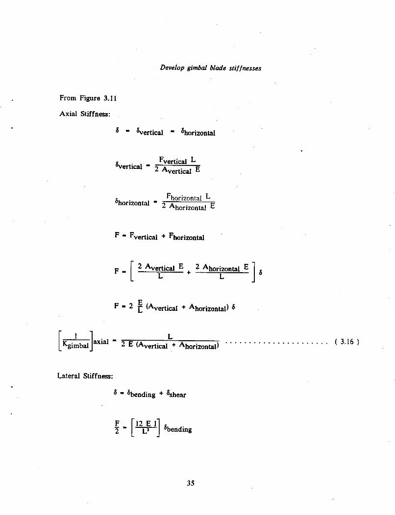
Develop gimbal blade stiff nesses

From Figure 3.1 1

Axial Stiffness:

bertical Shorizontal

Fhorizontal L *horizontal E &horizon tal =

2 *vertical E + Ahorizontal E F - [ L L 1

E F = 2 (Avertical + Ahorizontal)

...................... ( 3 . 1 6 ) L 2 E (Avertical + Ahorizontal)

Lateral Stiffness:

Sbending + !shear

- F [ T I 12EI Sbending 2

35

F G A 2 [T] %hear

. . . . . . . . . . . . . . . . . . . . . . . . . . . . ( 3 . 1 7 )

P L A C E S

H O R I Z O N T A

A j E j L V E R T I C A L

Figure 3.11 Gimbal Blades Configuration - - Axial, Shear and Bending

36

Develop frame stiffness

The frame stiffness described in Figure 3.12 and by Equations 3.18 and 3.19 was

not included in the SDOF analysis, as it was assumed that the frame was rigid in

comparison to the other structural elements in the flexure assembly. When the

NASTRAN model was assembled, actual section properties of all members were input.

When the NASTR.*AY m d e l predicted significantly lower natural frequencies than those

predicted by the SDOF model, the hand analysis described in Chapter 4 which included

the flexibility of the frame structure was performed. The results of the hand analysis

confirmed the NASTRAN model. but because the NASTRAN model was so close to a

final design, the SDOF model in the FORTRAN program in Appendix I was never

updated. Equations 3.18 and 3.19 are therefore included here for completeness of the

SDOF model.

From Figure 3.12

Bending and shear :

F = K S

s = 61 + s2 + 6, + 6,

62 = [:] [&I[+ - %) [+ + L1] ( Reference 6 )

37

( 3 . 1 8 ) Ls L12 + - J-s

[Kfr:meIwft I + 2 [ T - TI [k ]] 8 A G . . . . . . .

From Figure 3.12

Axial :

F - K 6

6 - 6 , + s ,

38 -. ...

F04

BENDINQ

Figure 3.12 Frame Configuration

39

1 Develop stability model

The flexure blades were designed to be as thin as possible to minimize the radial

stiffness, but the blades are still required to react the vertical shear and bending moment

imposed by the mass of the mirror vibrating parallel to the optical axis. Critical

buckling loads therefore had to be determined for each configuration considered.

Although closed form solutions with the proper boundary conditions were not available.

the closed form solutions which were available were all of the following form':

( 3.20 ) ts Fcr C B p.. . . . . . . . . . . + - - a . . . . . . . . . . . . . .

where:

FCr - critical shear load

B - blade height

t t blade thickness

L - blade length

C - constant, a function of boundary constraints

and material properties

Elastic stability models of selected flexure and gimbal blade configurations were run

on the NASTRAN finite element program. It was observed that the constant, C. in

Equation 3.20 could be extracted from the runs already made and that the deviation of

the critical load predicted from run to run was within five percent. Equation 3.20 was

incorporated into the SDOF parametric study program, thereby allowing the critical

I

I buckling load for each configuration studied to be calculated and compared with the

current working load without the need of making a NASTRAN run. Of course, the final

design configuration was analyzed for stability with NASTRAN, and a typical

NASTRAN input file for buckling is included in Appendix V.

40

Finalize SDOF program

All terms in Equations 3.7 and 3.8 have been determined and are described by

Equations 3.13 through 3.19. The remainder of the new program now takes on a

rearranged form of the old one. In summary:

Equation 3.4 gives the system stiffness:

K = 1.5 ( &oft + K k d

= 1.5 ( SKSSS + SKSSH )

Equation 3.3 gives the system natural frequency:

.

Equation 3.2 gives the value of the PSDF:

.02 x (386.4)2 ; if f S 250 hz or

.02 x (386.4)2 x [&] -1.993 ; if f > 250 hz

if f 5 250 hz, PSDF has slope of 0

if f > 250 hz, PSDF has slope of -6 dB

Equation 3.1 gives the RMS single axis PSDF displacement:

5 = 0.004

Ss, = 3 b l s

For two axis PSDF:

Gdesign 3 s s ~

Loads and stresses are then determined from the displacements. The output of

the updated parametric design program consists of the following items:

41

I A. Header: presents information on the current PSDF. damping ratio. flexure

~ material, cryogenic deflection, mirror weight and allowable operational bending

moment for the mirror.

Listing: following design parameters for each iteration considered. B.

1. Flexure blade length, width, and thickness.

2. Gimbal horizontal blade length. width.and thickness.

3. Horizontal displacement, (3a)

4. Vertical displacement, (3a)

5. Vertical natural frequency of SDOF system

6. Horizontal natural frequency of SDOF system

7. Vertical post load

8. Horizontal post load

C.

9. Margins of safety for:

a. Flexure in the hard direction

b, Flexure in the soft directioq

c. Gimbal in the hard direction

d. Gimbal in the soft direction

e. Bending moment at the mirror during cryogenic cooldown

f. Bending on vertical post

g. Manufacturing tolerances

h. Blade elastic stability (buckling)

The FORTRAN listing of the program used for the final design of the

SDOF system is presented in Appendix I.

42

A numerical example

The geometry of the final design submitted to NASA Ames is shown in Figure

1.5. That geometry will be used in determining the numerical values for SKSSS and

SKSSH in Equations 3.7 and 3.8. First the torsional stiffnesses, Krh and Krs will be

determined.

From Equation 3.5 :

2 G B , b S ( 3.5 repeated ) 2 G B, t, .................... K r h = [ 3 L l ’I+[ 3 L ] I 2.0 x 6.92 x IO6 x 3.0 x 0.19’ + 2.0 x 6.92 x lo6 x 2.0 x 0.143

3 x 3 3 x 3 = 3.164 x 10‘ + 8.439 x 10’

in-lb = 4.008 x 10 x.. . . . . . . . . . . . . . . . . . . . . . . . . . . . . . . ( 3.21 )

From Equation 3.6 : 4 G B, t,’ B, t: ........................ ( 3.6 repeated) Krs 3 B, t,’ L, + 6 b3 L,

I 4.0 x 6.92 x lo6 x 2.225 x 0.18s x 2.0 x 0.14s

3.0 x 2.225 x 0.18’ x 7.0 + 6.0 x 2.0 x 0.14’ x 6.0 = 4.193 x IOs s., . . . . . . . . . . . . . . . . . . . . . . . . ( 3.22 )

Now the vertical post stiffnesses:

From Equation 3.12 :

Where :

Kr = Krs or Krh , depending on direction

43


4 E I 4.0 x 18 x lP x r x 3.0' -I

L 64 x 3 7 in-lb * 9.538 x 10 x.. . . . . . . . . . . . . . . . . . . ( 3.23 )

As shown by Equations 3.21, 3.22, and 3.23 :

Therefore from Equation 3.13

[I-]rooft Kpost [&I 3.0 x 18.0 x lo6 x 3.0' + 6.92 x lo6 x I x 32

= [&]hard = ["I Kpost 2 [h + A] . . . . . . . . ( 3.13 repeated

3.05 x 64.0 3.0 x 4.0

~ - 3.951 x lo" + 6.136 x lo4 I

= 4.564 x IO-' E.. . . . . . . . . . . . . . . . . . . . . . . . . . . . . . . . . ( 3.24 )

Now the horizontal blade stiffnesses :


. . . . . . . . . . . ( 3.14 repeated ) 1 L'outer Iinner + 2 L'inner Iouter 48 E Iinner Iouter [ Kbl:des]mft =[

~

I 7.03 x 2.225 x 0.183 x 12.0 + 2.0 x 63 x 2.0 x 0.143 x 12.0 48.0 x 18.0 x 106 x 2.225 x 0.183 x 2.0 x 0.14'

= 1.330 x IO" E.. ................................. ( 3.25 )


. . . . . . . . . . . . ( 3.15 repeated ) Linner Aouter + 2 Louter Ainner 4 E Ainner Aouter 1

9 6.0 x 2.0 x 0.14 + 2.0 x 7.0 x 2.225 x 0.18 4.0 x 18.0 x lo6 x 2.225 x 0.18 x 2.0 x 0.14

= 9.025 x E.. . . . . . . . . . . . . . . . . . . . . . . . . . . . . . . . . ( 3.26 )

Now the gimbal blade stiffnesses :

44


1 L . . . . . . . . . . . . . . . . . ( 3.16 repeated ) [ Kgimbal]axial = 2 E (Avertical + Ahorizontal) I 3.0

= 9.804 x 10" E.. . . . . . . . . . . . . . . . . . . . . . . . . . . . . . . . . ( 3.27 )

(2.0 x 18.0 x IobX2.0 x 0.14 + 3.0 x 0.19)


[ 1 ]hard = [h] + [&I ...................... ( 3.17 repeated Kgimbal

I 3.OS x 12.0 3.0 24.0 x 18.0 x 106 x 3' x 0.19 + 2.0 x 6.92 x IO6 x 3.0 x 0.19

= 1.462 x 10-7 + 3.803 x 10-7 = 5.265 x . . . . . . . . . . . . . . . . . . . . . . . . . . . . . . . . . . . . ( 3.28 )


. ( 3.18 repeated ) LS

+ (4.5 - 1.44)2 (4.5 + 2.88)) 1 .o [96.0 x 18.0 x 106 x 0.0703

9 8.0 x 1.5 x 6.92 x 106 +

= 1.334 x 10" + 1.084 x lo-'

= 1.443 x 10" E.. . . . . . . . . . . . . . . . . . . . . . . . . . . . . . . . . ( 3.29 )


LS axial = .m ( 3.19 repeated ) 1 . . . . . . . . . . . . . . . . . . . . . . . . . . . . . . . . . [ K fr ame]

9.0 8.0 x 1.5 x 18.0 x IO6

I

= 4.167 x lo-' E.. . . . . . . . . . . . . . . . . . . . . . . . . . . . . . . . . ( 3.30 )

45

Now substituting Equations 3.24. 3.25 3.27 and 3.30 into Equation 3.7 :

I 1 1 1 -= SKSSS [ - Kkt]SOft +[ Kblades]soft +I jaxial +I k a m e ]axial Kgimbal

. . . . . . . . . . . . . . . . . . . . . . . . . . . . . . . . . . . . . . . . . . . . . . . . . . . (3.7 repeated)

~ = 4.564 x + 1.33 x IOe3 + 9.804 x + 4.167 .x IO-*

= 1.331 x 10-3

lb SKSSS = 751.5 - . . . . . . . . . . . . . . . . . . . . . . . . . . . . . . . . . . . . . . . . . . . . ( 3.31 ) in

I And substituting Equations 3.24, 3.26, 3.28 and 3.29 into Equation 3.8 :

[ l ] h a r d +[ ]axial +[ 1 ]hard +[ ]soft SKSSH Kpmt Kblades Kgimbal Kframe

. . . . . . . . . . . . . . . . . . . . . . . . . . . . . . . . . . . . . . . . . . . . . . . . . . . ( 3.8 repeated )

- 4.564 x IO-' + 9.025 x + 5.265 x + 1.443 x IO4

- 3.328 x 104 . lb SKSSH = 3.004 x 105 g . . . . . . . . . . . . . . . . . . . . . . . . . . . . . . . . . . . . . . . ( 3.32 )

At this point in the SDOF program, Equation 3.4 would be used to calculate the

system stiffness and Equation 3.3 would be used to calculate the natural frequency of the

system. When this is done with the values of SKSSH and SKSSS calculated above, the

frequency calculated is high by a factor of 1.89 when compared to the NASTRAN

results. This is explained by the coupling of the lateral translation mode with the

I rotation mode which is discussed in detail in Chapter 4 and observed in the NASTRAN

plots. The torsional mode of the mirror about its optical axis, however. is due entirely to

the SKSSH stiffnesses of each of the three flexure assemblies. Using NASTRAN this

torsional frequency is calculated to be 175 Hz as shown in Table 5.1. The following

analytical calculation to determine the natural frequency of the torsional mode using the

value of SKSSH calculated above demonstrates the validity of the modeling used in the

46

SDOF analysis.

From Figure 3.13 :

6 SO; M - J - R

6 and: 8 = - R M - J 8 ,

And:

M - 3 x F x R . and: F - K 6 SO: M I S X K X ~ X R

Giving:

J E = ~ x K x ~ x R s

J - 3 x K x R2

Where :

R - 13.0 inches


K = SKSSH = 3.004 x 1 0 5 in in-lb rad J = 1.523 x 108 -

Where :

Ipolar - 114.05 mugs-in2

f - 1 8 4 h z (NASTRAN analysis predicted 175 Hz)

47

J = Torsional Stiffness

M = Applied Torque

F = Force in Each Assembly

iwlar = Mirror's Polar Mass Moment of Inertia

Figure 3.13 Free Body for Torsion Model

48

Isolated modes of the flexure blades

Modes 4 through 9. as shown previously in Table 5.1. represent isolated

motions of the flexure blades only. Although no motion of the mirror occurs in these

modes, calculations of these frequencies are included here for completeness. The

model used to calculate those frequencies is shown in Figure 3.14.

M, = 21.0 x lo-' MUD

M, = 22.0 x IO-' Mugs

M, = 21.0 x 10-4 MUS

Figure .I4 Isolated

I, r (13+14+15)/3

L, = L,+L4+L,

des of Flexure Blades Ma

49

I Bending Stiffness

Shear Stiffness

~ 6 = 6, = 62 = s3

61 A10

Vl, - - L1

63 AlG v,, = - L1

62 A20

v2s = - J-2

I I

v, = [ T + 2A1G y] 6

2A1G A,G

2 x 0.28 x 18 x lo6 + 0.414 x 18 x lo6 I %=L, +r

I 7 x 2.6

in

6 x 2.6

= 1.03 x IO6

50

Total Stiffness

1 1 1 R = & + G 1 1

I-

1579 + - - 6.34 x lo-' &! lb K = 1577 in

Total Mass on Appendage

M = MI + M2 + M, = 64.0 x lo-' mugs

System Frequency

= 79.04 Hz. . . . . . . . . . . . . . . . . . . . . (NASTRAN analysis predicted 81 Hz)

51

CHAPTER 4

DYNAMIC ANALYSIS WITH A THREE DEGREE OF FREEDOM MODEL

The single degree of freedom model used during the parametric study of the

SIRTF design provided an accurate tool for analyzing the flexure system as long as the

vertical stiffness in the direction of the optical axis was mach greater than the lateral

stiffness. With the design evolution to the system of horizontal flexures, the vertical

stiffness decreased to a value less than the lateral stiffness which violated the basic

assumption of the SDOF model. As discussed in Chapter 3. the single degree of

freedom model still provided a configuration that allowed the final design to be

completed with very few NASTRAN iterations and it was not necessary to further

update the FORTRAN program. The numerical example presented in Chapter 3

demonstrated the accuracy of the modeling by predicting the natural frequency of the

torsional mode to be within 5.1 percent of the natural frequency predicted by the

NASTRAN analysis. Work presented ip this chapter was completed following the

final design of the SIRTF configuration and was prompted by the objective to better

define the coupling between the lateral and the rotational modes.

Although a FORTRAN program was not developed for the three degree of

freedom model discussed in this chapter, all stiffness equations developed could be

programmed for further parametric design studies should new requirements develop

from NASA Ames that would cause that effort to become necessary.

Develop the three DOF stiffness matrix

By inspection, the torsional mode is seen to be decoupled from the other

That decoupling was confirmed numerically in Chapter 3 as well as with the

Similarly, the vertical mode along the optical axis is seen to be

modes.

NASTRAN program.

52

decoupled from the other modes. However, the vertical mode will be included as one

of the degrees of freedom in this three degree of freedom model to consider the effects

of the dependence of the rotational stiffness on the vertical stiffness. Although those

two mode shapes are independent, the stiffnesses which determine their eigenvalues are

not. The three degree of freedom model is shown in Figure 4.1. The development of

the stiffness matrix for this system follows:

As shown in Figure 4.1 :

Unit displacement in the x-direction: 6, - I. all other displacements - 0.

Fx - K1, * Kh 6, - Kh

Fy = K2, - 0

= Ksl - Fx L = Kh 6, L - Kh L

Unit displacement in the y-direction: 6y - I , all other displacements = 0.

Fx = KI2 = 0

Fy - KZz - Kv aY = Kv

Me - Ksz - 0

Unit displacement in the B-direction: 8 = 1, all other displacements = 0.

53

Figure 4.1 Free Body Diagram of Three Degree of Freedom Model

54

Develop the eigenvalues

Characteristic equation :

( 4.1 1 A1 = - ... . . . . . . . . . . . . . . . . . . . . . . . . . . . . . . . . . . . . . . . . Kv m

Develop the relationship between K , and Kv

From Figure 4.2 :

M - Kt 8 . . . . . . . . . . . . . . . . . . . . . . . . . . . . . . . . . . . . . . . . . . . ( 4.3 )

And :

R M = F , R + Fz- . . . . . . . . . . . . . . . . . . . . . . . . . . . . . . . . . . . ( 4 . 4 )

55

= 3 ~ v 2 p = R K , R ~ 5

From Equations 4.3 and 4.4 :

M = R [ 5 ' K v R 8 ] + a [ ! j K v R 8 I = Kt 8

Kt = [!j K, R2 + K, R2]

Kt - 1 R2 K, . . . . . . . . . . . . . . . . . . . . . . . . . . . . . . . . . . . . . . . ( 4 . 5 )

x =

PLAN VIEW ELEVATION VIEW

Figure 4.2 Relationship Between IC, and Kt

56

A numerical example

Determine the vertical stiffness of a single flexure assembly as shown in Figure 4.3.

The geometry of the final design submitted to NASA Ames will be used in

numerically determining the vertical stiffness.

assembly is identified in Table 4.1 :

The load distribution throughout the

Axial deflection in post :

8 , = AE L F

F - 2.36 x 10‘ F 9 3 x 4 n x 32 x 18 x 106

Bending deflection in gimbal cruciform :

L’ F 6, - - 1 2 E I z 24 x 18 x l V x 0.14 x 8 F - 6.6% x lW7 F I 3’ x 12

Shear deflection in gimbal cruciform :

L F A G T

0.14 x 6.92 x lo6 x 2

6, = -

F = 1.548 x 1 0 6 F 3 I

Bending deflection in frame :

(2.88’ + 2 x (4.5 - 1.44)* (4.5 + 2.88)) F 12 I

96 x 18 x lo6 x 0.75 x8 = 1.876 x 10-7 F

Shear deflection in frame :

b F 2 A G 7

9 8 x 1.5 x 6.92 x lo6

Bending deflection in outer blade :

65 = - F = 1.084 x lo-’ F 9

L3 F & = m 7

7, x 12 = F = 4.253 x loa F 12 x 18 x lo6 x 0.14 x 8 x 4

57

0 I

\

0 >

Figure 4.3 Vertical Stiffness of Single Flexure Assembly

58

Shear deflection in outer blade :

L F A G Z 4 - -

F - 9.032 x lO-' F 7 4 x 2 x 0.14 x 6.92 x I@

I

Bending deflection in inner blade :

Ls F 12 E1 2 6, - -

I 63 x 12 F - 3.026 x IOa F 24 x 18 x 1V x 0.18 x 2.2253 Shear deflection in inner blade :

L F AG 3: 3, - -

F - 1.082 x loa F 6 0.18 x 2.225 x 6.92 x los x 2

I

Deflection due to torsional deflection of frame :

ML JG e - -

M - [$ x 71 x in-lb

J - 0.2813 in4

L - 3.06 in

s,, - 7 x e

Therefore :

F - 9.628 x IOa F 7= x 3.06 8 x 0.2813 x 6.92 x 106 'lo

LOCATION FORCE LOCATION FORCE 61 = Npost) F = &bending. outer blade) F/4 6, = G(bending, gimbal) F/2 S, - &shear, outer blade) F/4 6, = &shear, gimbal) F/2 s8 = &bending, inner blade) F/2 6, - &bending, frame) F/4 6, - &shear. inner blade) F/2 6, = &hear. frame) F/4 S,, - &torsion, frame) F/4

Table 4.1 Element loads for vertical stiffness

59

Flexure assembly vertical deflection :

6 = 6, + 6, + 65 + 6, + s5. + 66 + s, + 6, + 6, + s,,

= 2.143 x F

So. single flexure assembly force :

F = 4.666 x 10' 6

Vertical stiffness of SIRTF system :

lb Kv = 3 x 4.666 x lo5 - 1.40 x 105 7 in Vertical natural frequency of SIRTF system :

fl I 1 j - i x m 2n 0.668

= 72.9 Hz. . . . . . . . . . . . . . . . . . . (NAS"L4N analysis predicted 73 Hz)

Kt = 2 Kv . . . . . . . . . . . . . . . . . . . . . . . . . . . . . . . . . . . ( 4.5 repeated ) RZ

169 = - x 1.40 x 105 = 1.183 x lo7 !k 2 in From Equations 3.4 and 3.32 :

Kh - 3.004 X lo5 x 1.5 - 4.506 x lo5 lb I in I M = 0.668 mugs

I I = 57.47 mugs-in2 I I

From Equation 4.2

X, = 1.801 x lo5

I Therefore : I I f, = 67.6 Hz. . . . . . . . . . . . . . . . . . . (NASTRAN analysis predicted 69 Hz) I And :

X, = 7.709 x lo5

Therefore :

f3 = 140.0 Hz . . . . . . . . . . . . . . . . . . (NASTRAN analysis predicted 129 Hz)

1 60

CHAPTER 5

DYNAMIC ANALYSIS WITH A NASTRAN FINITE ELEMENT MODEL

The structural model used for the NASTRAN analysis is shown in Figure 5.1.

It has the center of the global coordinate system coinciding with the center post on one

of the flexure assemblies. It has the x-axis passing through the mid-plane of the right

center blade and the y-axis passing through the vertical projection of the mirror's

center of mass. Geometries for the other two flexure assemblies were obtained by

using the identical coordinates but in two newly defined Coordinate systems. One

coordinate system is rotated 1200 clockwise about the optical axis of the mirror and the

other is rotated 240'' clockwise about the same axis. Flexure assemblies were modeled

with beam (CBEAM) elements that included both flexure and shear stiffness. Fixity

was assigned to the center blade elements that interface with the SIRTF baseplate.

Rigid bar (MAR) elements were attached to the center posts of each of the three

flexure assemblies and connected at the center of mass of the mirror. Lumped

translational mass and mass moments of inertia were placed at the mirror's center of

mass to simulate the inertial effects of the mirror. Inherent in this modeling is the

assumption that the mirror and baseplate are much stiffer than the flexure assemblies,

as was established early in the system analysis.

- Solution Type 3 -- Normal Modes Analysis

Natural frequencies, mode shapes, and plots are available as output from SOL

3. Plots of the first twelve mode shapes are presented in Figures 5.2 through 5.13.

Mode 1, shown in Figure 5.2. is a lateral in-plane translation coupled with out-of-

plane rotation. It is one of the coupled modes discussed in Chapter 4. One flexure

assembly moves up while the other two move down. Mode 2. shown in Figure 5.3,

61

Figure 5.1 NASTRA Finite Element Model

has the same frequency as Mode 1 but is orthogonal to it. One flexure assembly is

essentially stationary while the other two are moving out of phase with each other

with equal amplitudes. These mode shapes occur at the same frequency because, as

was shown in the SDOF model, the stiffness of the entire support system is

independent of its orientation. This gives complete symmetry to the lateral and

rotational deflections even though the structure has three-fold structural symmetry

because of the three identical assemblies located 1200 apart. Identical frequencies are

62

Elevation View

FtLi.ll Plan View

Figure 5.2 NASTRAN Plot of Mode Shape 1 - 69 Hz

63

t

Isometric View

1

Elevation View

il 11 " I -

I w I

Plan View

Figure 5.3 NASTR4N Plot of Mode Shape 2 - 69 Hz

64

to be expected with any axes orientation used to model the assembly and the mode

shapes could be expected to change as a function of that orientation. The frequency

of mode shapes 1 and 2 was predicted by the three DOF model to within two percent

of the value calculated by NASTRAN. Mode 3, shown in Figure 5.4, is a pure

translation mode along the mirror's optical axis. The frequency of this mode shape

was predicted by the SDOF model to within one percent of the value calculated by

NASTRAN. Modes 4 through 9, shown in Figures 5.5 through 5.10. are modes with

the outer appendages of the gimbal oscillating. No motion of the mirror occurs.in

those modes.

within three percent of the values predicted by the NASTRAN analysis.

The frequencies of modes 4 through 9 were determined analytically to

Modes 10

and 11. shown in Figures 5.11 and 5.12. are the orthogonal complements of modes 1

and 2 in that they represent the coupled modes associated with the second root of the

quadratic characteristic equation. In both modes, one flexure assembly has very little

motion while the other two have larger motions of approximately the same magnitude.

In mode 10. the other two assemblies have motions that are in phase and in mode 11,

the other two assemblies have motions that are out of phase. The frequency of these

mode shapes was predicted by the three DOF model to within nine percent of the

value calculated using NASTRAN. Mode 12. shown in Figure 5.13. is a pure

torsional mode about the mirror's optical axis. The frequency of this mode shape was

predicted by the SDOF model to within six percent of the value calculated using

NASTRAN. Summarized in Table 5.1 are the values of the first twelve natural

frequencies of the flexure and gimbal assembly that were used to evaluate the system's

stresses and displacements. The input file for the SOL 3 analysis used for the final

analysis of the SIRTF configuration is listed in Appendix 11.

65

1

Isometric View

Elevation View

I

l h - Plan View

Figure 5.4 NASTRAN Plot of Mode Shape 3 -- 73 Hz

66

- I I I

1 I


67

Isometric View

Elevation View

4 H Plan View


68

Isometric View

Elevation View

Plan View


69

Isometric View

Elevation View

* Plan View


70

fscmetric View

Elevation View

I I- 1 I


71

Isometric View

Elevation View

p+-s Plan View


Isometric View

- 5 Elevation View

Plan View

Figure 5.1 1 NASTRAN Plot of Mode Shape 10 - 129 Hz

73

Isometric View

Elevation View

Plan View

Figure 5.12 NASTRAN Plot of Mode Shape 1 1 -- 129 Hz

74

Isometric View

Elevation View

Plan View


75

Natural Frequency

SDOF/SDOF NASTRAN Mode (W Comments

1

2

3

4

5

6

7

8

9

10

11

12

68

68

73

79

79

.79

79

79

79

140

140

1 84

Table 5.1

69 Lateral in-plane translation

69 and out-of-plane rotation

73 Optical axis translation

81 Flexure motion only






129 Lateral in-plane translation

129 and out-of-plane rotation

175 Torsion

First Twelve Natural Frequencies of SIRTF

Solution Type 63 -- Superelement Normal Modes Analysis

Solution Type 63 (SOL 63) was used to perform a complete dynamic design

I analysis based on the design criteria response spectrum. Applying the displacement

response spectrum dkr ibed by Equation 3.1 to the structure in each of the three

mutually orthogonal directions, a mode shape was determined by NASTRAN for each

of the twelve natural frequencies given in Table 5.1. Because of the symmetry of the

assembly, there are multiple eigenvalues as shown in Table 5.1. Consequently, the

method of combining modal maxima effects becomes a significant concern. Combining

.

I I 76

modal maxima effects by the square root of the sum of squares ( S W ) gives RMS

values providing that the eigenvalues are well spaced, however the SRSS method is

unconservative for systems that have repeated eigenvalues. Combining modal maxima

effects by the sum of the absolutes (ABS) is appropriate if all of the eigenvalues are

essentially equal. The Naval Research Laboratory (NRL) method of combining modal

maxima effects applies if the lowest mode is the dominant mode and the remaining

modes are well dispersed. Each of the above three methods is available in NASTRAP!

but none of them are actually appropriate for the SIRTF assembly. A fourth method

called CLOSE is also available in NASTRAN. The user is required to define a value

for the variable "close". Each eigenvalue is compared to the one that precedes it and

if their difference is equal to or less than the value "close". then those two modal

maxima associated with those two eigenvalues are added absolutely. If the eigenvalue

difference is greater than "close", the modal maxima associated with the larger

eigenvalue is included in an SRSS combination and the procedure is repeated for the

next eigenvalue comparison.

The limited methods of combining modal maxima is not unique to the

NASTRAN program. It is a problem that exists for most large computer programs in

use today'. A method for combining modal maxima effects using a displacement

response spectrum that gives essentially the same results as obtained using a power

spectral density criteria was developed in this design study. This result' is the

Modified Root of the Sum of the Squares (MRSS) method. It is a variation of the

CLOSE method available in NASTRAN. The value for "close" in MRSS is

determined from the cross-modal coefficients, pij. For SIRTF. the coefficients can be

approximatedg as the cross-correlations between modal responses given by:

77

where r = 2. For constant modal damping, {, this becomes: wj

312 8f2 (l+r)r . . . . . . . . . . . . ( 5 . 2 ) pij ( I -9)2+4tZr( 1 +r)2

For a given damping ratio, these equations may be used to determine when

the eigenvalues are essentially equal.

The procedure for using MRSS is as follows:

1: Make a SOL 3 run on NASTRAN to determine the system's eigenvalue

distribution.

2: Identify eigenvalues that are "close".

3: Make the following analysis using SOL 63:

a: Identify in the NASTRAN input file, those specific eigenvalues

that are close and select the option in NASTRAN that combines

their modal maxima effects with ABS.

b: Identify in the NASTRAN input file, those specific eigenvalues

that are well spaced. For each individual eigenvalue, select

the option in NASTRAN that calculates its modal maxima effects.

Either ABS or SRSS can be selected here as they give the same ,

result for a single eigenvalue selection.

c: External to NASTRAN, using data obtained above. combine by

SRSS the results of the ABS combinations with the results of the

distinct eigenvalue cases.

The accuracy of the MRSS method of combining modal maxima for the SIRTF

flexure assembly is demonstrated in Table 7.1 where the MRSS design loads are

summarized with the SOL 30 design loads. Equations that define the methods for

.

i combining modal maxima effects are shown in Figure 5.14.

78 I

SRSS method: ( Up ) = 1 2 ( Up2 li’ H >I ( I up I )

P l

Absolute method: ( Up ) =

NRL method: ( Up ) = [ I ul I 3 + H >: ( up2 1

Z - CLOSE method: ( Up 1 = >. ( I up I ) +

P-1

MRSS method: ( Up ) =

Where:

pz+ 1

Up = Combined response

up = Response of mode p

H

Z

N

K

= Number of modes considered in the analysis

= Total number of modes determined to be close

= Number of sets of equal or close eigenvalues

= Number of equal or close eigenvalues in any set

Figure 5.14 Modal Response Combinations

79

A numerical example fo1lows that demonstrates the methods for combining

modal maxima that have been presented. The histogram of the first twelve

N u m k c r r 6 - - 4 09

E l q w n v c r l u w r

frequencies for SIRTF is shown in Figure 5.15 to emphasize the MRSS combination

scheme. After each grouping is summed absolutely, the summations of each group are

combined by SRSS. For the example, it will be assumed that the effect of each modal

maxima is the same and that each has a value equal to one. The results indicate

that the conclusion of a response spectrum analysis depends strongly on the modal

maxima combination scheme selected.

SRSS - (12+12+12+12+12+12+12+12+12+12+12+12)1~2 = JTZ = 3.46

-- - - - = n

ABS - 1+1+1+1+1+1+1+1+1+1+l+l = 12.00

CLOSE = 10 + (12 + l2)ll2 = 11.41

I MRSS I (22+12+62+22+12)1/2 = a = 6.78 i I I

~ 80

Solution Type 30 - - Modal Frequency Response Analysis

Solution Type 30 is both more complex and more expensive to use than SOL

63 to perform random vibration analysis in a design made, but SOL 30 is also

expected to provide the more accurate solution. The significant difference in effort

and complexity between SOL 63 and SOL 30 is in the post processing of the

frequency response analysis. Following the SOL 30 frequency response analysis. the

power spectral density curves of the response quantities are determined based directly

on the input PSDF and are integrated to provide the Rus values of the response

quantities. For the SIRTF analysis those response quantities were displacements and

loads. The SOL 30 analysis is expected to produce the best solution of all the solution

types considered, with the only error resulting from the numerical integration scheme

within the computing process. A comparison of results is shown in Table 7.1.

The burden of defining the integration intervals of the power spectral density

curves is left to the user of NASTRAN. This requires that a plot of the function to

be integrated be made in order to determine the frequency range over which the

function has significant magnitude as well as to determine the integration intervals.

Two typical PSD plots from the SIRTF analysis are shown in Figures 5.16 and 5.17.

As can be explicitly seen from those plots, the curves to be integrated are essentially

spikes and care must be taken to insure that the integration is done accurately. Small

errors in the selection of the integrating parameters for systems such as SIRTF with

low damping can easily result in large errors in the final design parameters.

81

ORIGINAL PAGE 1s OF POOR QUALITY

' .c

I .tJ -

Figure 5.16 Typical Deflection PSD Plot from SOL 30

82

ORiGlNPL PAGE IrS OF POOR QUALITY

r r >' 3 , - ' U

Figure 5.17 Typical Internal Load PSD Plot from SOL 30

83

CHAPTER 6

A COST COMPARISON OF THE SIRTF DYNAMIC ANALYSIS

Although designing an acceptable configuration for the support structure of the

SIRTF primary mirror was the w i n objective of this study, minimizing the costs

involved in performing the dynamic analysis was an issue that became a secondary

objective. Many flexure wsembly configurations were considered in this design study.

Clearly, the budget constraints for this project would not have allowed those iterations

to have been made using only NASTRAN. This chapter contains a summary of the

costs incurred for each of the solution types used in this study. The value received

for a given investment of resources is highest for the SDOF/3DOF models providing

that accurate modeling is assured. The modest cost of a full NASTRAN analysis

using the MRSS combination scheme with SOL 63 is attractive when compared to the

costs of a SOL 30 NASTRAN analysis, That is especially so when the results are

shown to be nearly the same as demonstrated in Figure 7.1. The MRSS combination

scheme with SOL 63 provides the best NASTRAN alternative based on the SIRTF

design study.

A subjective cost item not included in this summary is the hourly manpower

rate of the user in applying the various methods discussed. Once the SDOF/3DOF

design model is constructed, it requires the least amount of experience of the user.

SOL 63 could easily be used by a junior level engineer provided proper supervision is

available. SOL 30 is difficult to use with many different ways to obtain an erroneous

conclusion. A clear understanding of random vibrations is required of the user as this

portion of NASTRAN is not well documented. Manpower costs, then, can vary in the

progression just presented based solely on the experience required of the user.

84

Cost of analysis with the FORTRAN model

Previous workg on the SIRTF configuration had just developed a preliminary

FORTRAN program that considered the system to behave as a single degree of

freedom. It

could have as easily been written to operate on a PC as very little storage is required

for its operation. On the University of Arizona computer center's VAX, each iteration

of several hundred configurations cost less than two dollars. On a PC the cost would

be zero if the initial cost of the PC is ignored. As all data input to the computer

systems were input through a PC. the initial cost of the PC is common to all of the

procedures considered and will be ignored. Manpower costs for preparing input to the

FORTRAN model is negligible when cost per configuration evaluated is considered. A

thirty minute session could result in as many as five hundred configurations being

analyzed. The manpower costs for evaluating the output are also minimal as only

those configurations that passed all of the system requirements are presented in the

output. The primary manpower cost was in developing the initial program and then

updating it for the different fundamental configurations. Each major update required

a supplemental hand analysis for confirmation of the programming accuracy. Over the

eighteen month duration of this design effort, approximately five major programming

iterations took place with approximately sixty manhours of programming and

confirmation calculations per iteration. An estimated three thousand configurations

were considered and most of them were unacceptable. That is approximately 0.1

manhour per configuration studied.

That program was modified to FORTRAN 77 for the VAX computer.

Cost of analysis with the NASTRAN SOL 3 model

The cost of the typical SIRTF configuration on a SOL 3 NASTRAN analysis

SOL 3 models are was approximately three dollars on the University's Cyber system.

85 -. ...

very similar to static analysis models and they provided the nodal geometry and

connectivity for the SOL 63 and SOL 30 models that followed. Geometry plots were

obtained from this model as well as mode shape plots for each natural frequency. No

specific dynamic loads analysis is performed with SOL 3, however, the frequencies

calculated are useful in checking both the FORTRAN model and the other NASTRAN

models. A direct comparison can be made with the frequency calculated with the

SDOF/3DOF models and if they agree, it can be concluded that both were modeled

correctly. The check with the other NASTRAN models has value because the

eigenvalues result from different analytical models within NASTRAN. SOL 3 models

have the ground points fixed as in a statics analysis. That is equivalent to the

support being a stiff spring, resulting in a high frequency mode that is ignored in the

output. SOL 30 and SOL 63 models require the introduction of a large mass to

represent ground. All fixed points must be attached to the large mass by rigid

members. The introduction of the large mass results in a low frequency, essentially

zero. mode shape for each degree of freedom associated with the large mass.

Reproducing the frequencies calculated with the SOL 3 option provides conformation

that the SOL 63 and SOL 30 input file have been correctly assembled because the

determination of the values of that large mass and its mass moments of inertia are

non-trivial efforts. The cost of the SOL 3 analysis is included in the model

development costs of the SOL 63 and SOL 30 costs. so the SOL 3 analyses will not be

summarized separately m this cost comparison.


The time required to develop a NASTRAN model of a typical SIRTF model is

approximately forty hours. Each analysis requesting the SRSS or ABS combination

scheme cost eleven dollars. Minor changes in configuration do not require an

86

accompanying SOL 3 analysis. For each SOL 63 analysis, six deflections were

calculated at each node and all loads within each element were calculated. This is

important in comparing costs with SOL 30 'as the cost for a comparable amount of

output with SOL 30 would have been prohibitive for this project.

As stated in Chapter 5, neither the SRSS nor the ABS combination schemes

are applicable to SIRTF. Although the MRSS scheme introduces slightly higher costs

than SRSS or ABS, the MRSS combination scheme provided a more accurate solution

for SIRTF. From the SOL 3 analyses, the modal groupings are determined for the

SOL 63 MRSS analyses. Following those analyses, an SRSS combination is done by

hand. Automating that combination scheme could easily be done, but for the SIRTF

design it was done by hand. Each ABS combination scheme grouping cost

approximately nine dollars resulting in a composite MRSS cost of forty-five dollars per

analysis. The manhours to manually perform the subsequent SRSS by hand was

approximately four hours for SIRTF. Automating that process would allow the same

amount of data to be combined as is obtained from a normal SOL 63 analysis and it

would take significantly less than four hours to accomplish. For SIRTF, only that data

that was determined to be important was actually combined by SRSS following the

SOL 63 ABS analyses.


The SOL 30 option in NASTRAN is difficult to use. It performs the same

frequency response analysis used in SOL 63 but it then integrates the power spectral

density function of the response desired producing an RMS value of that response.

Those integrating parameters are left for the user to define. For SIRTF the functions

being integrated were typically spike functions where a small error in defining the tip

of the spike or a small error in the integrating interval resulted in a very significant

87

1 error in the value of the integral. Plots of the power spectral density functions of the

desired responses were required in order to define the range and the value of the

integrating intervals. Although, raster plots are relatively inexpensive. their quality was

generally not acceptable so Calcomp plots were required. Procedures for requesting

output from SOL 30 analyses are awkward. Each deflection desired and each load

desired is a special request and each requires an individual plot for defining the

integrating parameters. The primary cost of this solution type is in the integrating

scheme. Of the 2,568 responses available that were all reported by the SOL 63

analysis, 148 responses were requested in the SOL 30 analysis. The cost of the SOL

30 analysis was $68.00 for CPU and $320.00 for plots. Actual manhours devoted to

establishing the first acceptable analysis are not included in this cost comparison as a

significant amount of time was spent in learning to use the SOL 30 option in

NASTRAN. The preprocessing time presented is an estimate of the time that it would

take to do it a second time. It must be kept in mind that even though SOL 30 is the

hardest option to use of those considered; properly applied. it is expected to give the

most reliable output for design.

Cost summary of anaZyses

The summary of the discussions of the previous sections is presented in Table

6.1.

88

Manhour summary

Model

SDOF/3DOF

SOL 63 - SRSS

SOL 63 - ABS

SOL 63 - MRSS

Sol 30

Model Development Preprocessing

New configuration Per iteration (manhours) (manhours)

60.0 0.0

40.0 8.0

40.0 8.0

40.0 12.0

50.0 16.0

Post-processing Per iteration (manhours)

0.0

0.0

0.0

4.0

16.0

Cost summary

Number of Model Computer Plotter Iterations

(dollar) (dollar) Analyzed

SDOF/3DOF 0.0 0.0 3.000

SOL 63 - SRSS 11.0 4.0 10

SOL 63 - ABS 11.0 4.0 10

SOL 63 - MRSS 45.0 4.0 5

Sol 30 68.0 320.0 I

* Assumes basic configuration already exists and only an iteration analysis is made.

Processing Costs per

Iteration (*) &/iteration dollar/iteration

20.0 0.0

8.0 15.0

8.0 15.0

16.0 I 49.0

32.0 388.0

Table 6.1 Cost Comparison of the SIRTF Dynamic Analysis

89

CHAPTER 7

SUMMARY AND CONCLUSIONS

Methods used in developing the final design configuration of the support

structure for the primary mirror of the Space Infrared Telescope Facility (SIRTF) have

been presented.

A brief description of the work performed with FRINGE was presented in

Chapter 2. This work was necessary in order to establish the maximum loads that the

support structure could apply to the mirror during operation at cryogenic temperatures.

This began by modifying the program FRINGE to accept as its input. the output from

the structural analysis program NASTRAN. The interfacing of these two programs

allows an optical evaluation to be made of the structural deflections on the optical

surface of the mirror. By applying unit loads to a finite element model of the mirror

at the points which interface with the support structure. influence coefficients were

obtained relating surface deflections on the mirror to unit loads at the support

interface. For SIRTF. NASA had prepared an optical error budget that established the

limit of the Rh4S deflections allowed on the optical surface. Comparing those limits

with the results of the FRINGE program allowed the unit loads to be ratioed to

establish a set of design loads for the support structure. In performing that analysis it

was determined that the bending moment at the plane of the mirror's centroid was the

load of concern. The shear accompanying the bending moment has a negligible

influence with respect to that of the bending moment. Combining the maximum load

that the mirror can withstand during optical operation with the known deflection that

occurs during cryogenic cooldown leaves only the stiffness of each flexure assembly as

the design variable. Radial compliance was a constant consideration throughout this

I

I

I

90

design effort.

The dynamic design analysis began using the three point support concept

established on previous work performed at the University of Arizona for NASA Ames.

A presentation demonstrating that the three point support system behaves as a single

degree of freedom is shown in detail in Chapter 3. It is further shown that the

system stiffness in the lateral direction can be expressed as a function of the sum of

the radial stiffness and tangential stiffness of a single leg in the three leg support. If

the radial stiffness is significantly less than the tangential stiffness, the system stiffness

becomes a function of only the tangential stiffness. This approach was taken in the

selection of some of the early design considerations as it was necessary to limit the

radial stiffness to meet the cryogenic cooldown requirements. Early attempts were

made to decouple the radial stiffness and the tangential stiffness by using the concept

of a parallel spring guide. The inherent coupling of that configuration made it an

unacceptable design. Manufacturing tolerances generated constraints that had to be

satisfied. Mismatch of components during manufacturing caused the same type of

aberrations to the optics as the moments resulting from cryogenic cooldown. A

torsionally compliant gimbal structure placed between each leg of the flexure assembly

and the baseplate solved the manufacturing tolerance problem. This gimbal structure

evolved into a successful configuration for significantly decoupling the radial and

tangential stiffnesses. Buckling of the various components was fully considered. Euler

buckling was a problem for the long blade design, but the folded back configuration

solved that problem. Out of plane buckling due to shear remained an item of concern

throughout this design effort. An algorithm for predicting the critical buckling load

was developed for the FORTRAN parametric analysis and the final design was

analyzed for stability with a special NASTRAN analysis.

91

Demonstrating that the system could be considered as a SDOF allowed a straight

forward parametric design program to be written in FORTRAN. Expense in both

manhours and computer time was minimized by using this program to parametrically

identify available design space. Accuracy of the simplified FORTRAN analysis was

checked regularly with a NASTRAN modal. In the early designs that had a relatively

simple structure, the results of the FORTRAN analysis were consistently within five

percent of the results predicted by the NASTRAN model. As the configurations

became more complex, the accuracy decreased. Specifically. as the design approached

its final configuration, the stiffness of each flexure assembly along the mirror's optical

axis decreased, thereby allowing the rotational mode of the mirror assembly to couple

with the lateral mode. The coupling modes and frequencies were described by a three

degree of freedom model shown in Chapter 4. Although the equations presented were

not programmed, the hand calculations presented demonstrate that the problem is well

understood. If new design constraints were to be applied to the SIRTF telescope,

these equations could be programmed and used for further parametric studies.

Developing the FORTRAN program to investigate preliminary designs provided a cost

effective method to evaluate many different configurations. Developing the stlffness

equations for the FORTRAN program further resulted in a more thorough

understanding of the effect of each element in the SIRTF support structure. Typical

of the insights provided by the SDOF was the ability to decouple the radial and

translational stiffnesses and still have a structurally stable system.

.

I

In addition to the SDOF and the three DOF models, dynamic analysis was

performed using three different capabilities of NASTRAN. SOL 3 was used to

determine the natural frequencies and mode shape plots of the system. SOL 63 was

used to perform a displacement response spectrum analysis. which led to the subject of

combining modal maxima of closely spaced modes. The SRSS, ABS. and CLOSE

92

methods available within NASTRAN were discussed. None of the available methods

offer satisfactory results. ABS is inherently too conservative for modes with well

spaced natural frequencies. SRSS is unpredictable for modes with clustered natural

frequencies and can predict unconservative results. CLOSE was considered and a

similar approach to CLOSE was developed for the SIRTF design which is presented as

MRSS. It can be expected

to give near exact solutions. however it offered its own set of complications.

Establishing the integrating interval for SOL 30 is a non-trivial procedure.

SOL 30 was used to perform the final dynamic analysis.

In summary, the MRSS method of combining modal maxima effects resulting

from a SOL 63 analysis with NASTRAN gave almost identical results as the SOL 30

results. The comparisons were made on the design loads at the glass to titanium

interface at the mirror socket and on the maximum design moments on the flexure

support assembly. These results are shown in Table 7.1.

93

Socket loads

Method

Moment Shear

(in-1 b) (lb)

S R S 35.500

ABS 69,600

MRSS 45,100

SOL 30 45.000

11.800

23,300

15,100

15,000

Axial

(Ib)

5,300

9,400

5,800

5.600

Blade loads

Method

SRSS

ABS

MRSS

SOL 30

Outer moment Inner moment

(in-lb) (in-lb)

5.987

1 1 . 1 0 0

6,783

6,336

1 1,922

22,149

13.560

12.650

Table 7.1 Numerical Summary of Dynamic Analysis

94

REFERENCES

1. Melugin, R. K. and Miller, J. H.. Infrared Telescope Design: Implications from

Contemporary Cryogenic Tests of Fused-silica Mirrors. SPIE Proc. 433 (1 983).

Methods of Optical Manufacturing and Testing.

2. Vukobratovich, D.. Iraninejad. B., Richard, R. M.. Hansen, Q. M., and Melugin, R..

Optimum Shape for Lightweighted Mirrors, SPIE Proc. 332 (1982). International

Conference on Advanced Technology Optical Telescopes.

3. Iraninejad. Bijan and Vukobratovich. Daniel, Double Arch Mirror Study. Engineering

Analysis Report, NASA Grant 2-220, NASA Ames Research Center, Mail Stop

244-7, Moffett Field, California 94035, May 1983.

4. Neugebauer, George H.. Designing Springs For Parallel Motion, Machine Design,

Volume 52: 1 19-120, August 7,1980. .

5. Crandall, Stephen H. and Mark, William D.. Random Vibration, Academic PressJnc.,

Orlando, Florida, 1%3.

6. Roark. Raymond J. Formulas For Stress And Strain, Fifth Edition, McGraw-Hill.

New York. 1975.

7. Timoshenko, Stephen P. and Gere, James M.. Theory Of Elastic Stability. McGraw-

Hill. New York. 1961.

8. Richard, R. M.. Private Communication, University of Arizona, 1987.

9. Wilson, E. L., Der Kiureghian. A., and Bayo, E. P., A Replacement for the SRSS

Method in Seismic Analysis. Publication of University of California, Berkeley,

California.

APPENDIX I

FORTRAN LISTING OF SDOF DESIGN STUDY

C VANMARCKE’S EQUATION FOR A SDOF SYSTEM C EQUATIONS ASSUME SINGLE CYLINDER VERTICAL POST, A TWO C CRUCIFORM GIMBAL, AND TWO SOFT FLEXURES, EACH C CONSISTING OF 3 BLADES C MAY 6. 1987 C C BY WAYNE POLLARD AND MYUNG CHO C

PROGRAM BLOCK CHARACTER ITIME*S,IDATE* 14 CHARACTER* 1 9 CHA.CHB.CHC.CHD.CHE,CHF,CHG.CHH,CHI,CHJ.CHK,CHL

PO-MAXIMUM VALUE OF PSD INPUT (IN/SEC2)2/HZ C C C YM=YOUNGS MODULUS PSI C SIGMA-ALLOWABLE STRESS PSI C C SGSLOPE OF PSD C E-PERCENT CRITICAL DAMPING C WEIGHTIMIRROR WEIGHT C ZARM-MOMENT ARM FROM GIMBAL PLANE TO MIRROR CG C CRYDEG RADIAL THERMAL SHRINKAGE OF BASEPLATE C GMSHEAR MOD (SET TO LARGE VALUE TO EXCLUDE SHEAR DEFORMATION) C

FO-LIMIT OF CONSTAN SPECTRAL DENSITY

OPEN(UNIT=6,FILE=’BLWK.DAT,STATUSI’OLD) OPEN(UNIT=7,FILE=’BLOCK.OUT’,STATUSI’NEW’)

C

C C IF ISIZE - C EQ.l ONE METER MIRROR C NE.1 HALF METER MIRROR C C IF JUMPSF - C C EQ.0 NO CHECK C C ALL - ALLOWABLE SAFETY FACTOR (DEFAULT 1.0) C C C C IF IOPT - C EQ.l VERTICAL BLADE OF CRUCIFORM IDENTICAL TO HORIZ BLADE C EQ.0 VERTICAL BLADE OF CRUCIFORM IDENTICAL TO SOFT

READ(6.111) ISIZE.JUMPSF,ALL,STB.IOPT

I

EQ.l CHECK FACTOR OF SAFETY

STA - SAFETY FACTOR FOR STABILITY (3 SIGMA)

96

BLADE C 1 1 I FORMAT(/215,2FS.0,15)

IF(ISIZE.EQ. I ) THEN CRYDEG.062 WEIGHT1258. CRYMOM=74.7 WRITE(7.'(///,25H *** ONE METER MIRROR ***)') WRITE(7.'(

CRYDEG .0324 WEIGHT=35. CRYMOM-30.4 WRITE(7.'(///.26i-i *** HALF METER MIRROR ***)*)

15H NOTE: CRYDEL 1.F6.3)') CRYDEL ELSE

ENDIF C C** CONSTANTS C

XMASS=WEIGHT/386. PSb.02 E d 0 4 PoIPSD*386.*386. YM- 18000000. GMmYMJ2.6 SIGMA- 129000. FO-250. SG-6.0

C WRITE(7.89)PSD.YM,GM.SIGMA,E,CRYMOM, WEIGHTCRYDEL

+/,* SHEAR MODULUS= '.E8.3./.' ALLOWABLE !3TREssI ',E8.3./.

+' THERMAL SHRINKAGE OF BASEPLATE= ',F7.3, +//,' VERTICAL FLEXURE IS A SINGLE CIRCULAR POST'/)

89 FORMAT(//.* PSD= '.F8.3,/,' MODULUS OF ELASTICITY= '.E10.5.

+' CRITICAL DAMPING RATIO= ',F7.4./,' ALLOWABLE CRY0 MOMENT= '. +F7.3./.' MIRROR WEIGHT- '.F7.3./,

CALL DATE(1DATE) CALL TIMQITIME) WRITE(7.899) ITIMEIDATE

WRITE(T. 1 14) ISIZE.JUMPSF.ALL,STB.IOPT 899 FORMAT(/// 1 X,30( 1 H*)/' THIS RAN AT '.A5,' ON ',A 14/ 1 X,30( 1 H*))

1 14 FORMAT(///,' ISIZE ='.123X,'JUMPSF ='.12,3X,'ALL =',F5.2. + 3X.'STB =',F5.2,3X.'IOPT =*J2)

C POST DIMENSIONS READ(6.999) FL1 ,FL2.FL3.FBI .FB2,FB3.FT1 .FT2.FT3

C SELECT OUTER FLEXURE BLADE DIMENSIONS, SOFT READ(6.999) GL I ,GL2,GL3,GB 1 ,GB2.GB3.GT 1 ,GT2,GT3

READ(6.999) GLX 1 .GLX2,GLX3,GBX 1 ,GBXZGBXS,GTX 1 ,GTX2,GTX3

READ(6.999) GLC 1 ,GLC2,GLC3,GBC I ,GBC2,GBC3,GTC 1 ,GTC2,GTC3

CHA=' POST LENGTH'

C SELECT GIMBAL BLADE DIMENSIONS, HARD - HORZ. CRUCIFORM BLADES

C SELECT INNER FLEXURE BLADE DIMENSIONS

C

97

CHI&' POST DIAMETER' CHC=' POST THICK CHI)I' FLEX SOFT LENGTH' CHE-'FLEX SOFT WIDTH' CHF='FLEX SOFT THICK' CHI=' GIMBAL HARD LENGTH' C H G GIMBAL HARD WIDTH' C"=' GIMBAL HARD THICK CHJ=' FLEX CENT LENGTH' CHK='FLEX CENT WIDTH' CHG'FLEX CENT THICK' WRITE(7.997) WRITE(7.998) CHA,FLI ,FL2,FL3,CHB,FBI ,FB2.FB3,CHC,FTI .FT2.FT3 WRITE(7.998) CHD.GL1 ,GL2.GL3.CHE,GB 1 .GB2,GB3.CHF,GT1 ,GT2,GT3 WRITE(7.998) CHLGLX 1 .GLX2.GLX3.CHG,GBX 1 .GBXZGBX3.

WRITE(7.998) CHJ.GLC 1 ,GLC2,GLC3,CHK,GBC I .GBC;?.GBC3,

997 FORMAT(///,22X,' START LAST STEP') 998 FORMAT(/.A I 9.3X.3F8.3) 999 FORMAT(/.3FS. 0)

+ CHH,GTX 1 .GTXZGTX3

+ CHL,GTC 1 .GTC2,GTC3

C C** JUMPSF=l NO CHECK FOR SAFETY FACTORS, OTHERWISE CHECK C** ALL IS ALLOWABLE SAFETY FACTOR, SET ALG1.O C C FGPOST LENGTH

C FB=POST OD

C FT=POST WALL THICKNESS

DO 100 FGFLl.FL2.FL3

DO 100 FB.IFBI.FB2.FB3

DO 100 FT=FTI,FT2.FT3 ZARMIFL

WRITE(7.901) FL.FB,FT 901 FORMAT(////,' FL = ',F5.2.' FB = ',F5.2,' FT = ',F5.3)

C GLX=GIMBAL LENGTH. HARD DO 100 GLX-GLX 1 .GLX2,GLX3

C GBXICiIMBAL WIDTH, HARD DO IO0 GBX=GBX 1 .GBX2,GBX3

C GTXlGIMBAL THICKNESS, HARD DO 100 GTX-GTXI.GTX2.GTX3

WRITE(7.902) GLX.GBX,GTX

I

I 902 FORMAT(////,' GLX = ',F5.2.' GBX = ',F5.2,' GTX = ',F5.3) WRITE(7.900)

900 FORMAT(/.' GL GB GT GLC GBC GTC VDISP . +. "DISP VFREQ HFREQ VUNIT HUNIT FH' +r ' GH GS CC VBH VBS TM SS')

C SELECT OUTER FLEXURE BLADE DIMENSIONS C GGFLEXURE LENGTH, SOFT

DO 100 GGGLl.GL2.GL3 C GbFLEXURE WIDTH, SOFT

I 98

DO 100 GB-GBI.GB2.GB3 C GT=FLEXURE THICKNESS. SOFT

DO 100 GT-GTI.GT2.GT3 C SELECT INNER FLEXURE BLADE DIMENSIONS C GLX=FLD<URE LENGTH, CENTER C DO 100 GLC=GLC 1 .GLC2,GLC3

C GBX=FLEXURE WIDTH. CENTER GLCeL- 1.

C DO 100 GEK=GBCI,GBC2,GBC3

C GTX=FLEXURE THICKNESS, CENTER

C GIMBAL ROTATIONAL STIFFNESS SOFT, GKRS

GBC=GB

DO 100 GTC=GTCl .GTC2.GTC3

GJI=GB*(GT*3)/3.0 GJ2=GBC*(OTC**3)/3 .O GKRSI(GM*4.0*GJ 1 *GJ2)/(GL*GJ2+2.0*GLC*GJ I)

C GIMBAL ROTATIONAL STIFFNESS HARD, GKRH GKRH=(GM*4.0*GBX*GTX**3 J/(3 .O*GLX) IF (IOPT .NE. 1 ) GKRH=GKRH/2. +(GM*2.0*GB*GP*3 .)/(3 .O*GLX)

GINER 1 =GB*GT**3. / 1 2. GINER2=GBC*GTC**3/12. GKTSSA=((GL**3)*GINE2+2.*(GLC**3)*GINER 1 )/(48. *YM*GINER 1 *GINER2)

I +(GL*GBC*GTC+2.O*GLC*GB*GT)/(4.O*GM*GBC*GTC*GB*GT) INCLUDE STIFFNESS OF BLADE LENGTH GKTSSGKTSSA+GLX/(4*YM*GBX*GTX) IF (IOPT .NE.

C GIMBAL TRANSLATIONAL STIFFNESS. I/KT. SOFT

C

1 )GKTSS=GKTSSA+GLX/(2*YM*GB*GT)+GLX/(2*YM*GBX*GTX) C GIMBAL TRANSLATIONAL STIFFNESS, 1/KT, HARD

GINER-(GTX*(GBX)**3 .+GBX*GTX**3 .)/ 12. IF (IOPT .NE. l)GINER=(GTX*(GBX)**3.+GB*GT*3.)/12. GKTSH=GLX**3./(24.*YM*GINER)+GLX/(2.*(GBX)*GTX*GM)

C GKTSH=GK?ISH+(GL*GBGTC+2.O*GLC*GB*GT)/(4.O*YM*GB*GT*GBC*GTO

C FLEXURE INERTIA, HARD FIH=( 3.1 4 1 5 9/4. )*(( FB/2 .)**4. -(FB/2 .-FT)**4.)

C FLEXURE INERTIA, SOFT FIS-FIH

C POST HEIGHT PH--(FL-ZARM)

C ASSEMBLY STIFFNESS. HARD PAR I =3.0*PH/(2.*FL)

C WRITE(7,’(/6H PARl=.G11.3)’) PAR1 PAR2=1 .O+GKRH*FL/(4.O*YM*FIH)

C WRITE(7.’(/6H PAR21.Gll.3)’) PAR2 PAR3=FL**3./( 12.*YM*FIH)

C WRITE(7,’(/6H PAR31.Gl1.3)’) PAR3 SKSSHI=( 1 .+PAR 1 /PAR2)*PAR3*(PAR2+PARl)/(PAR2-.75)

C WRITE(7,’(/8H SKSSHI=,GI 1.3)’) SKSSHI

C WRITE(7,’(/8H SKSSHb.Gll.3)’) SKSSHI

INCLUDE !3TIFFNEss OF BLADE LENGTH

SKSSHI=SKSSHI+(PH**2.*FJJ(4.*YM*FIH))/PAR2+GKTSH

99

SKSSHISKSSHI+FL/( 3.1 4*(( FB/2 .)**2-( FB/2. -FT)**2. )*GM)

SKSSH= 1 ./SKSSHI C WRITE(7.'(/8H SKSSHI-,GI 1.3)') SKSSHI

C WRITE(7,'(/8H SKSSH =.G11.3)') SKSSH C ASSEMBLY STIFFNESS, SOFT

C WRITE(7,'(/6H PAR21.Gl1.3)') PAR2

C WRITE(7,'(/6H pAR3.1.Gl1.3)') PAR3

C WRITE(7.'(/8H SKSSSb.Gll.3)') SKSSSI

C WRITE(7,'(/8H SKSSSL.Gll.3)') SKSSSI SKSSSISKSSSI+FL/( 3.1 4*((FB/2 .)**2-(p/2. -Fl3**2 .)*GM)

C WRITE(7,'(/8H SKSSSb.Gll.3)') SKSSSI SKSSS-1 JSKSSSI

C WRITE(7,'(/8H SKSSS -,GI 1.3)') SKSSS C WRITE(7.81)EL C 81 FORMAT(//////,' LENGTH-',F6.3.//) C WRITE(7.99) C 99 FORMAT(2X,TREQUENCY',6X,'PSD,SX,'DISPLA~W~2X. C +' I1 1 ',4X.'SHEAR'.7X.'MOM,8X.*~,1OX,'H, C +lOX,'I22',8X.*AREA',6X.' J'./.39X,'(LARGE)',17X.'(CRYO)') C C SYSTEM STIFFNESS

C SDOF FREQUENCY

C PSD VALUE

PAR2-1 .+GKRS*FL/(4.O*YM*FIS)

PAR3=FL**3./( 12.*YM*FIS)

SKSSSI=( 1 .+PAR1 /PAR2)*PAR3*(PAR2+PARl)/(PAR2-.75)

SKSSSISKSSSI +( PH*+2. *FL/(4. *YM*FIS))/PAR2+GKTSS

SYS-l.5*(SKSSS+SKSSH)

F-1./(2.*3.14159)*SQRT(SYS/XMASS)

IF(F.LE.250.m TO 90

GO TO 91 S=PO*(F/FO)**(SL*3.32 19/10.0)

90 S-PO 91 CONTINUE

C RMS DEFLECTION. SINGLE AXIS PSD

C RMS DEFLECTION, TWO AXIS PSD

C 3 SIGMA DEFLECTION, 2 AXIS PSD

C SYSTEM SHEAR TO BE COMPARED TO EIGENVALUE IN STABILITY RUN

C ASSEMBLY SHEAR, TWO AXIS PSD

C BENDING STRESS IN FLEXURE, HARD

C WRITE(7,'(/6H BMFHI.Gl1.3)') BM

D+/( 1 984. *E*P*3 .))**. 5

DSYS=1.414*D

DsYS=3.*DsYS

SYSSHR=DSYS*SYS

ASHEAR=DSYS*SKSSH

BM=ASHEAR*FL/2.

FSH=BM*FB/(2.0*FIH) SAFEFHSIGMA/FSH

IF(JUMPSF.NE. 1 .AND. SAFEFH.LT.ALL) GOT0 100 C BENDING STRESS IN GIMBAL, HARD: SHEAR DIVIDES TO TWO BLADES

100

BM-(ASHEAR*GLX/2.)/2.

GSH=BM*(GBX/(2.))/(((GBX)**3.*GTX+GTX**3.%BX)/l2.) IF (IOPT .NE. 1 )GSH=BM*(GBX/(2.))/(((GBX)**3. *GTX+GT**3. *GB)/ 1 2.) SAFEGH=SIGMA/GSH

C WRITE(7.’(/6H BMGHI.Gl1.3)’) BM

IF(JUMPSF.NE. 1 .AND. SAFEGH.LT.ALL) GOTO 100 C RADIAL SHEAR FOR CRY COOLDOWN

C BENDING STRESS IN FLEXURE, SOFT C BM=RSHEAR*FL/2. C WRITE(7,’(/6H BMFS.Gl1.3)’) BM C FSS=BM*FB/(2. *FIS) C SAFEESISIGMA/FSS C BENDING STRESS IN GIMBAL, SOFT: SHEAR DIVIDES TO TWO BLADES

RSHEAR-CRYDEL*SKSSS

BM-(RSHEAR*GLC/2.)/2. C WRITE(7.’(/6H BMGSI.Gl1.3)’) BM

GSS=BM*(GT/2.)/(GB*GP*3./12.) SAFEGSIGMA/GSS

IF(JUMPSF.NE. 1 .AND. SAFEGS.LT.ALL) GOTO 100 C BENDING MOMENT AT MIRRORS CG C INCLUDES GB/2.

CGMOM=RSHEAR*(ZARM+GB/2.) SAFECC=CRYMOM/CGMOM

IF(JUMPSF.NE. 1 .AND. SAFECC.LT.ALL) GOTO 100 C VERTICAL STIFFNESS OF A GIMBAL ASSEMBLY

GINERl-GT*GB**3/12.0 GINER2=GTC*GBC**3/ 12.0 GKVII-(2.*GLC*+3.%INERl +GL**3.*GINER2)/(48.*YM%INERl *GINER2)

1 +(~.*GLC*GB*GT+GL*GBC*GTC)/(~.*GPGB*GM*GBC*GTC)

IF (IOPT .NE. 1) GKVIIGKVII+GLX**3./(2.*YM*GPGB**3.) 1 +GLX/(2. *GT*GB*GM)

GKVI=GKVII+GLX**3./(2.*YM*GTX*GBX**3.)+GLX/(2.*GTX*GBX*GM)

GKV- 1 ./GKVI

SYSGKV=3.*GKV

vF-(1./(2.*3.141 59))*(SYSGKV/XMASS)**.5

IF (VF.LE.250.)GO TO 700 VSPO*(vF/FO)**(SL*3.32 19/10.) GOTO 910

C VERTICAL STIFFNESS OF SYSTEM

C VERTICAL NATURAL FREQUENCY

C CHECK POINT ON PSD CURVE

700 VS-PO 910 CONTINUE C VERTICAL RMS DISPLACEMENT

VD=(VS/( l984.*E*W*3.))**.5 C VERTICAL 3 SIGMA DISPLACEMENT

vD=3.*vD C VERTICAL SHEAR. SINGLE ASSEMBLY

VSHEAR=SYSGKV*VD/3. C VERTICAL BENDING MOMENT SOFT: SHEAR DIVIDES TO TWO BLADES

VBMS-(VSHEAR*GLC/2.)/2. C VERTICAL BENDING STRESS SOFT

101

VBSSIVBMS*(GB/2.)/((GT*(GB)**3 ./ 12.)) SAFVBSSIGMA/VBSS

IF(JUMPSF.NE. 1 .AND. SAFVBS.LT.ALL) GOTO 100 C VERTICAL BENDING MOMENT HARD: SHEAR DIVIDES TO TWO BLADES

C VERTICAL BENDING STRESS HARD VBMHdVSHEAR*GLX/2.)/2.

VBsH=VBMHYGBX/2.)/((GTx*(GBX)**3./12.)) IF (IOPT . NE. l)VBSH=VBMH*(GB/2.)/((GTGB**3.+GB**3.+GBX*GTx**3.)/12.) SAFVBHSIGMA/VBSH

IF(JUMPSF.NE. 1 .AND. SAFVBH.LT.ALL) GOTO 100 C TORSIONAL MOMENT ON GIMBAL/MIRROR DUE TO .001 RAD MISALIGNMENT

TMMH=GKRH*.001 TMMS=GKRS*.OOl TMM=AMAX 1 (TMMH.Th4MS) TMM=TMM/2. SAFTMM=CRYMOM/TMM

IF(JUh.IPSF.NE. I .AND. SAFTMM.LT.ALL) GOTO 100 C STABILITY ALGORITHM

SSYS=VSHEAR/(Z. *GB*GT**3/GL**2) SK=2837./6.173E-5

C F A n O R OF SAFETY ON STABILITY

C FS 1 =SK/SSYS

SSYS=VSHEAR/(GBC*GTC**3/GLC**2) SK=2837./6.173E-5

C FACTOR OF SAFETY ON STABILITY FS2SK/SSYS FS=FSl IF (FSl .GT. FS2)FS=FS2

IF(SAFXFH .GT. 9.) SAFEFH=9.0 IF(SAFEGH .GT. 9.) SAFEGH19.0 IF(SAFEGS .GT. 9.) SAFEGS19.0 IF(SAFECC .GT. 9.) SAFECC=9.0 IF(SAFVBH .GT. 9.) SAFVBH=9.0 IF(SAFVBS .GT. 9.) SAFVBS9.0 IF(SAFTMM .GT. 9.) SAFTMM=9.0 IF(FS .GT. 9.) FS 19.0 IF(% .LT. STB) GOTO 903

C

888 WRITE(7.905) GL,GB,GT,GLC,GBC,GTC,VD,DSYS.VF.F,VSHEAR,ASHEAR +r

SAFEFH,SAFEGH.SAFEGS.SAFECC.SAFVBH.SAFVBS,SAFIMM,FS 903 CONTINUE 905 FORMAT(1X.2(2F5.2,F6.3).6E10.3.7FS.lFF4.1)

100 CONTINUE STOP END

102

APPENDIX I1

NASTRAN INPUT FILE - - SOLUTION TYPE 3

ID SIRTF,FREQ SOL 3 TIME 50 CEND TITLE- SIRTF 1.0 M - TAPERED(2.Oe2.45). I"ER=O.18; OUTERIO.14 THICK SUBTITLE-DYNAMICS FOR Wt=258 LB MIRROR SPC-23 DISPLACEMENT - ALL METHOD-1 OuTPuT(PL0T) PLOTTER NAST SET I = ALL

FIND SCALE. ORIGIN 1, SET 1 PLOTSET 1,ORIGIN 1

PLOT MODAL DEFORMATION 0 RANGE O..300.,SET 1.SHAPE AXES Y,Z,X VIEW O..O.,O. FIND SCALEORIGIN 2.SET 1 PLOT MODAL DEFdRMATION 0 RANGE O..300..SET 1,ORIGIN 2,SHAPE AXES ZX.Y VIEW O..O.,O. FIND SCALE,ORIGIN 4,SET I PLOT MODAL DEFORMATION 0 RANGE 0..300..SET 1.ORIGIN 4.SHAPE BEGIN BULK Program listing begins double column here CBEAM ,191.4.1 12.191.501 GRID ,294.1, 6.75.0.0.0.0

CBEAM .193,5,193,194,501 GRID ,392.2.4 75.0.0,O.O CBEAM .I 94.4.194.13 1.501 GRID ,393.2, 4.75.0.0.0.0 CBEAM $29 I .4.2 12.29 1 ,SO 1 GRID ,394.2. 6.75,O.O.O.O CBEAM ,292,5,29 1.29230 1 CBEAM ,293.5.293.294.50 I CORD2R,I,O,11.26.19.50,0.0,11.26,19.5.1.0.+ CBEAM ,294,4,294,23 1 ,SO 1 CBEAM .391,4,312.391,501 +RD1,0.0,39.0.0.0 CBEAM ,392.5.39 1,392.501 CORD2R,2,0,-11.26.19.5,0.0,-11.26,19.5,1 .O,+ CBEAM ,393.5,393,394.501 RD2 CBEAM ,394,4,394.33 1,501 +RD2.- 15.01.13.0.0.0 GRID .191.0.-6.75,0.0.0.0 GRID , I 92,0,-4.75,0.0,0.0 PBEAM ,1.1.1.SOO..0703,.5000,0.0..2813 GRID ,193.0. 4.75.0.0.0.0 1 $2.1. .280.4.6-4,.0933,0.0,.00 18 GRID ,194.0. 6.75,O.O.O.O 1 ,3,1, .387..0010..1491,0.0,.0042 GRID ,291.1,-6.75,0.0.0.0 = ,4.1. .441 ,.OO 12..2206,0.0,.0048 GRID ,292.1,-4.75,O.O.O.O = S.1. .414..0011..1825,0.0..0045 GRID ,293.1, 4.75,0.0,0.0 = ,6,1.1.838,.086 1 ..9191,0.0..3445

UNDEFORMED MESH

DEFORMED MESH

CBEAM ,192,5,191,192,501 GRID ,391.2,-6.75.0.0.0.0

RDl

103

I ,7,1, .850,.4280..0950.0.0,.0087 I .9.1.7.069,3.976,3.976.0.0,7.952

CONM2, 101.500.0.0.668 ..,.. +COW2 +COW2.57.4761,,57.4761,,,114.0531 EIGR,l,MHOU,10.0,600 .,.,,, +EIGR1 +EIGRl ,MAX

MATl,l.18.0+6,,.3 SPC1.23 ,123456.1 16.127 SPC 1.23 ,123456.2 16.227 SPC 1.23 ,123456.3 16,327

PARAM,AUTOSPC.YES RBAR. IO 1,500,12 1,123456,,, 12345 1

RBAR. 102,500.22 1,123456,,, 123456 RBAR, 103SOO.32 1,123456... 123456 RBAR. 1 12,120.122,123456... 123456 RBAR, I 14,122.123,123456,,, 123456 RBAR. 21 2.220.222.123456.,, 123456 RBAR. 2 14.222.223.123456... 123456 WAR, 3 12.320.322.123456,,, I23456 RBAR, 3 14,322,323,123456,,, 123456 PLOTEL,500 1.500,12 I PLOTEL*5002,5OO,22 1 PLOTEL.5003,500.32 1

1 ST CMASS2.1111.21.0-4,111,3 --

.*(I I.= .I 13.3

.*( 1 ).= , 130.3

.*( 1 I*= ,132.3

.*( 1),22.0-4.112,3

.*( 1 ),= ,131.3

.*(1).16.8-4,114.3

.*( 1 ).= -1 18.3

.*(I ).= ,125.3 **( 1 I.= ,129,3 .*( 1).27.6-4.115.3 .*( 1 ).= ,117.3 **( 1 1,- ,126.3 .*( 1 )*= ,128.3 .*(1).18.2-4.119.3 ,*( 1 ).= , 124.3 .*( 1).5.%-4,120.3 .*( 1 I.= ,123.3

.*(1),5.60-4,116,3

.*( 1 I.= ,127.3

.*( 1),18.3-3.122.3

. , 2 ND ------

cMAss2.2 1 1 1.2 I .0-4.2 I 1.3 I **( 1 I*= .2 13.3 .. ,*( 1 I.= ,230.3

I .*( 1 I*= ,232.3 I .*( 1),22.0-4,212,3 I .*( 1 I*= -23 1.3 I ,*( 1). 16.8-4,2 14.3 I .*( 1 ).= ,2 18.3 I .*( 1 )*= ,225.3 I .*( 1 I.= ,229.3 .. ,*( 1),27.6-4,2 15.3 I .*( 1 I,= ,2 1 7.3 I .*( 1 I.= ,226.3 .. .*( 11.9 ,228.3

I .*( 1 I.= ,224.3 I ,*( 1)s. 94-4,220,3 .) .*( 1 ).= ,223.3

I .*( I ),5.60-4,2 1 6.3 I .*( 1 I*= ,227.3

3 RD CMASS2.3 I 1 1.2 1.0-4.3 1 1.3 I .*( 1 ).= ,3 13.3 = .*( 11.- ,330.3 I .*( 1 ).= ,332.3

= .*( 1 I*= .33 1.3 I .*( 1 ), 1 6.8-4.3 1 4.3 I **( 1 ).= ,3 18.3 I **( 1 )I= .325,3 I .*( 1 ).= ,329.3 I .*( 1),27.6-4.315.3 I .Y l)*= ,317.3

.*( 1 I*= ,326.3 I .*( 1 ).= ,328.3

= .*(I I.= ,324.3 = .*( 1),5.94-4,320.3 I ,*( 1 ).= ,323.3

I .*( 1). 18.2-4.2 19.3

I .*(I). 18.3-3.222.3

I .*( 1).22.0-4.3 12.3

I .*( 1). 18.2-4.3 19.3

I .*( 1). 18.3-3.322.3 ;II .*( 1),5.60-4.3 16.3 I .*( 1 ).= ,327.3

2- 1 cMAss2,1211.21.0-4.111,2 I ,*( I).= ,113.2 I .*( 1 ).= ,130.2 I .*( 1 I.= ,132.2

= .*( 11.9 ,131.2

I .*(I).= ,118.2 I **( 1 I.= ,125.2 I .*( 1 I.= ,129.2

---

I .*( 1),22.0-4.112.2

= ,*(1).16.8-4.114.2

I ,*( 1).27.6-4.115.2

104

I .*( 1 I.= ,I 17.2 I .*( 1 I*= ,126,2 = .*( 1 I.= ,128.2 I .*(1).18.2-4.119,2 I **( 1 ).= ,124.2 I .*(I ),5.94-4,120,2 I ,*( 1 I.= ,123.2

I .*( 1 ),5.60-4.116,2 I .*( 1 )I= ,127.2

cMAss2.22 1 1.2 1.0-4.2 1 I ,2 I .*( 1 ).I ,2 13.2 I .*(I ).I ,230.2 I .*(I ).I ,232.2 I .*( 1 ),22.0-4,2 12.2 I .*( 1 I.= .23 I .2 I ,*(1),16.8-4,214,2 I .*( 1 ).I ,2 I 8.2 I .*(I).= ,225.2 I .*(I).- ,229.2 I .*( 1),27.6-4,2 15.2 I .*( 1 I.= .2 1 7.2 I .*( 1 ).I ,226.2 I .*( 1 ).I ,228.2 I .*(1).18.2-4.219.2 I .*( I).- ,224.2 I .*( 1 ),5.94-4,220.2 I .*(I I*= ,223.2

I .*( 1 ).5.60-4.216.2 = .*( I).- ,227.2

3 R D CMASS2.321 I ,2 I .0-4,3 1 1.2

I ,*( 1),18.3-3,122,2

2 N D

I .*(I). 18.3-3.222.2

**(I ).= ,3 13.2 .*( 1 )*= ,330,2 .*(I I.= ,332.2 .*( 1).22.0-4,3 12.2 .*( 1 I.= .33 1.2 .*(I), 16.8-4.314.2 .*( 1 ).= ,3 18.2 .*( 1 I.= ,325.2 .*(I ).= ,329.2 .*( 1).27.6-4.3 15.2 **( 1 ).I ,3 17.2 **( 1 ).= ,326.2 **( 1 )*= ,328.2 ,*( 1),18.2-4,319,2 .*(I I.= ,324.2 ,*( 1),5.94-4.320,2 .*( 1 ).= ,323.2 ,*( 1). 18.3-3.322.2

I .*( 1).5.60-4.3 16.2 I . **(l).- ,327.2

CMASS2,1311,21.0-4.111.1 I .*( 1 I.= , I 13.1 = .*( 1 ).= ,130.1 I .*(I).- ,132.1 I ,*(1).22.0-4,112.1 I ,*( I).- ,131.1 I ,*(I). 16.8-4.1 14.1 I .*( 1 I*= ,118.1 = .*( 1 I.= ,125.1 I .*(I ).I ,129.1 I .*(1).27.6-4.115,1 I .*( 1 I.= ,I 17.1 I .*( 1 I.= ,126.1 I .*( I)*- ,128.1 I .*(I), 18.2-4, I 19. I I **( 1 ).= ,124.1 I .*(1),5.94-4.120.1 I .*( I).- ,123.1

I ,*(1).5.60-4.116.1 I .*(I I.= ,127.1

CMASS2.23 1 1.2 1.0-4.2 1 1.1 I .*( 11.- ,213.1 I ,*(I ).= ,230.1 = .*(I).- ,232.1 I .*( 1).22.0-4.212,1 I .*(I ).= ,231.1 I .*( 1). 16.8-4.2 14, I I .*( 1 I.= ,218.1 I .*( 1 ).= ,225.1 I ,*( 1 ).= ,229. I I .*(1),27.6-4,215,1 .. .*( 1 ).= ,217.1 I .*( I).- ,226.1

.Y 1 I.= ,228.1 I .*(1).18.2-4,219,1 = .*( I).- ,224.1 I .*( 1),5.94-4.220. I .. .*( 1 I.= ,223.1

I .*( 1).5.60-4.216.1 I **( 1 ).I ,227.1

3 RD CMASS2.33 1 1.2 1.0-4.3 1 1.1 = .*( I).- ,313.1 = .*(I).- ,330. I I **( 1 ).I ,332.1 I .*( 1).22.0-4.312.1

3- 1

I .*(I), 18.3-3.122.1

2 N D

I

I ,*(1),18.3-3,222.1

105

.*( 1 ).= ,331.1

.*( 1). 16.84.3 14.1

.*( I I.= ,318.1

.*( 1 1.- ,325.1 **( 1 1.- ,329.1 .*( 1),27.6-4,315,1 .*( 1 1.- ,317.1 .*( 1 1,- ,326, I **( 1 I.= ,328.1 ,*( l), 18.243 19,l .*( 1 ).- ,324.1 .*( 1).5.94-4,320.1 .*( 1)P ,323.1

.*( 1),5.60+,3 16.1

.*( 1 1.- ,327.1

.*(I), 18.3-3,322,l

1ST CBEAM , 11 1.6.1 I 1 , I 12.501

,*(1),6,112,113,- .*( 1).2.111 1 15,- .*( 1),3, 192,116,- .*( 1),2,113,117,= ~~1)~1,114.115.- ,y1).=.115,117,- .*( 1).=. 1 1 7.1 18.- .*(1).-.114,119.- .*(I).-. 1 19,125.- .*( 1).7.119.120.131 , 123.9.12 1,122,501 , 125.7,123,124,13 1 , 127.1.1 18,124,501 ,*( 1 ) ~ . 124.129,- .*(I),=, 125,126.- .*(I).=. 126,128.1 .*(I),=, 128.129.- .*( 1),2,126,130,= .*( 1),3,127. 193.- .*( 1),2, 128,132,- .*( 1),6,13 1.1 30.1 12 .*( 1).6.132,13 1 ,lI2

2 ND -- CBEAM I 21 1.6.21 1.212,501 = .*(1),6.212.213.=

**( 1).2.2 1 1.2 1 5*= 3 ,*( 1).3,292.216.- I .*( 1),2.213.217,- I .*( 1). 1.2 14.2 1 5,- I .*( 1),-,2 15.2 1 7.1 .. .*( 1),-,2 1 7.2 18,= I .*( 1),-,214,2 19.- I .*( 1),-,2 19.225.-

m

.. .*( 1),7.219,220,23 1 I , 223.9.22 1,222.50 1 - , 2257,223,224.23 1 I , 227.1.2 18,224.50 1 I .*( 1).-,224,229,- = .*( 1),-,225,226.- I .*( 1).-,226.228.1 I ,*( 1 ).=,228.229,= I .*( 1).2,226.230.- I .*( 1).3.227,293.- = .*( 1).2.228,232.= I .*( 1),6,23 1.230.2 12 I .*( 1).6,232.23 1.2 12

3 RD CBEAM , 3 1 1.6.3 1 1.3 12.50 1 I .*( 1),6.3 12.3 1 3.- = .*( 1).2,3 1 I ,3 15,- I .*( 1).3,392,3 16,- I ,*( 1).2,3 13.3 17.1 = .*(1).1.314.315,- I ,*(1).-,315,317,- = ,*( 1),=,3 17.3 18,= I ,*( 1),-,3 14.3 19,- I .*( 1),=,3 19,325.- .. .*( 1).7,3 19,320.33 1 = , 323.9.32 1,322.50 1 I , 325.7.323.324.331 = , 327. I .3 18,324,501 I .*( 1),=,324.329,- = ,*( 1).=,325,326.- I .*( 1 ),=,326.328,- = .*( 1),=.328.329.= .. ,*( 1),2.326,330,= = .*( 1),3.327.393,= = .*( 1).2,328,332,= I ,*( 1).6,33 1,330.3 I2 I .*( 1).6,332.331,312 CBEAM , 101.6,101,111.501 m .*( l),-* 1 I3,102,= I .*( 1).-, I 30,103,- = .*(I),-, 104,132,- CBEAM , 20 1.6.20 I ,2 1 1 S O 1 .. ,*( 1),-,2 13.202.1 = .*( 1).-.230.203.- I ,*( 1).-.204,232,= CBEAM , 30 1.6.30 1.3 1 1 ,SO 1 = .*( 1),-,3 13.302,- I .*( 1),=.330,303,- .. .*( 1),-.304.332.-

GRID, 101.0.-8.75 , 2.88 ,O.O - .*(l).-.- ,-2.88 ,a

106

,*(I),=, 8.75 2.88 = .*(l).=.- ,-2.88 .= GRID, 201,1,-8.75 . 2-88 .O.O = .*(l).=.= .-2.88 .I = **(I),=, 8.75 , 2.88 = **(l)*=.= .-2.88 .I GRID, 301,2.-8.75 . 2.88 90.0 - .*(1).=.= ,-2.88 p = ,*(l)p. 8.75 * 2.88 P - **(l)*=*- ,-2.88 .= GRID, 500.0, 0.0 ,13.0 -3.0 GRID, 501.0. 0.0 ,13.0 $0.0

1 ST ---- GRID, 11 1,0,-8.75 . 1-44 90.0 = **(l).=.= , 0.0 *- = **(l)*-.= 71.44 *- = , 130,=. 8.75 . 1.44 .- = .*(1).-.= * 0.0 *- = .*(l).=.- ,-1.44 *- = , 114,=,-1.75 , 4.5 $0.0 - ,*(l),=,= 1.44 ,= = .*(1),=,-2.75 * 0.0 9.1

= 9*(1),=,-1.75 ,-1.44 = .*(1).=.= 4 . 5 .= = , 125p, 1.75 I 4.5 = **(l).=.= , 1.44 ,= = **(l)p* 2.75 , 0.0 = ,*(l)p. 1.75 .-1.44 .I - **(l).=.= 4 . 5 .- = , 119p. 0.0 . 4.5 P

= .*(l).=.= I 1.5 ,= * **(l)*=.= , 0.0 $3.0 = .*(l).=.= , 0.0 .o.o = **(l).-.= .-1.5 *= = **(l).=.= 74.5 *=

2 ND GRID, 211,1,-8.75 . 1-44 8.0 = .*(l)*=.= * 0.0 *- - **(l)*=.= ,-1.44 *== = , 230.1. 8.75 . 1.44 3-

= **(I).=.= * 0.0 *- = .*(l).-.- .-1.44 .- = .*(l).=.= , 1.44 .=

= ,*(1).=.-1.75 .-1.44 = ,*(l)*=.- 4 . 5 ,= = , 225,-, 1.75 4.5 P - ,*(l)*=.= , 1.44 ,= = ,*(l)p. 2.75 , 0.0 P

= ,*(I),=, 1.75 ,-1.44 .= - .*(l).=*= ,-4.5 .=

= , 214,=,-1.75 , 4.5 90.0

,*(1).=.-2.75 , 0.0 9.1

= , 219.1. 0.0 . 4.5 - **(l).=*- . 1.5 .- = .*(l)*-.- * 0.0 ,3.0 = **(l).=*- , 0.0 .o.o = .*(l)*=,- .-1.5 .- = .*(l)*=.- $4.5 .-

3 R D

= **(l).-.= , 0.0 .- - ,*(l).-*- 71.44 ,==

= .*(1)*-.- 0.0 .- = .*(l).=.- 71.44 *- = 314,=.-1.75 * 4.5 .O.O = .Yl).-.- , 1.44 .= = **(1),-,-2.75 0.0 .I = .*(1),=+-1.75 ,-1.44 ,I - **(l).=.- A . 5 ,= = , 325.1. 1.75 , 4.5 ,= - *Yl)*=.- 1.44 ,- = ,*(l)p, 2.75 , 0.0 *- - .Y1)*=. 1.75 ,-1.44 ,I = **(l)*=*- .-4.5 *= = 319.1, 0.0 , 4.5 *= = .*(l)*=.- I 1.5 ,- - *Yl)*=.= , 0.0 .3.0 = **(l)*-.- * 0.0 .o.o = ,*(l)*-.- .-1.5 ,= = ,Yl).=.= *-4.5 .= ENDDATA

GRID, 311,2,-8.75 1.44 -0.0

- , 330.-,, 8.75 , 1.44 .-

107

APPENDIX 111


ID SIRTF,SPECTRUM SOL 63 TIME 10 ALTER 5 DBSTORE SPECSEL//V,Y,SOLID/O CEND

BLADES

DISPLACEMENT = ALL ELF0 = ALL DLOAD = 1 METHOP. 1 S E T 1 1 0 SEALL = 1 BEGIN BULK

TITLE.. SIRTF TAPERED DEPTH(2-2.45); 0.18 INNER BLADE - 0.14 OUTER

SUBTITLESPECTRUM 1 M (Wt1258 LB) - ABS (0 - 200 HZ)

Program listing begins double column here CBEAM ,191,4,112.191,501 CBEAM ~192.5.191,192,501 CBEAM ,193,5,193,194.50 1 CBEAM ,194,4,194,131,50 1 CBEAM .29 1.4.2 12.29 1.50 1 CBEAM ,292.5.29 1,292.50 1 CBEAM ,293,5,293,294,50 1 CBEAM ,294.4.294.23 1.50 1 CBEAM ,391.4,312,391.501 CBEAM ,392.5.39 1,39230 1 CBEAM ,393,5,393,394.50 1 CBEAM ,394.4.394.33 I .50 1

GRID $1 92.0.4 75,O.O.O.O GRID ,193.0. 4.75.0.0,O.O GRID ,194.0, 6.75.0.0.0.0 GRID .291,1.-6.75,0.0,0.0 GRID .292,1.-4.75,0.0,0.0 GRID ,293.1, 4.75.0.0.0.0 GRID ,294,1, 6.75.0.0,O.O GRID .39 1,2.-6.75,0.0,0.0

GRID ,393.2, 4.75,O.O.O.O GRID ,394.2. 6.75,0.0,0.0

GRID ,191.0,-6.75,O.O.O.O

GRID ,392.2,-4.75.0.0.0.0

CORD2R,1,0.11.26,19.50.0.0,11.26.19.5.1 .O,+ RD 1 +RD1,0.0,39.0,0.0

108 - --

CORD2R,2,0.-11.26.19.5,0.0,-11.26,19.5.1 .O,+

+RD2.-15.01,13.0.0.0 RD2

PBEAM , 1 ,l ,1.500..0703,.5000,0.0,.2813 I .2.1, .280,4.6-4..0933.0.0,.00 18 I ,3,1, .387,.0010..1491,0.0..0042 = .4.1, .44 1 ,.OO 12,.2206.0.0,.0048 I S.1. .414..0011,.1825.0.0..0045 I ,6.1,1.838..0861,.9191,0.0..3445 = ,7,1, .850,.4280,.0950,0.0,.0087 I .9,1,7.069.3.976,3.976.0.0.7.952 MAT1,1,18.0+6,,.3 SUPORTSO 1,123456 CMASS2,333.1.+6 ,50 1.1 I ,334,- .= .2 I ,335.1 *= ,3 CMASS2.336.1.+8 ,50 1.4 I ,337,- ,= ,5 I ,338,- ,= .6

CONM2.101 SOO.O.O.668 .,,.. +CONM2 +CONM2,57.476 137.476 1 ,,, 1 14.053 1 EIGR.l,MGIV,10.0.300 .,.... +EIGRl +EIGRl .MASS DLOAD.1,1.,1.,1,1.0,1,1.0,1,+DLOAD +DLOAD,O.O,1,0.0.1,0.0,1 DTI.SPECSEL.0

DTI.SPECSEL. I ,,D, 1 ..004.ENDREC RBE2,901,501,123456,116,127.216,227,316,+R BE +RBE327 TABLED 1 * 1 .....,..+ TAB 1 +TAB1, 40.,7.668-2, 50.,5.487-2, 60.,4.174-2, 80.,2.711-2,+TAB2 +TAB2,100..1.940-2.150.,1.056-2,200..6.858-3 .230..5.561-3,+TAB3 +TAB3,260.,4.450-3.290..3.388-3.320..2.650-3 ,350..2.118-3.+TAB4 +TAB4,ENDT PARAM.SCRSPEC,O PARAM.LFREQ.0. PARAM.HFREQ.200. . PARAM,OPTION,ABS

1 ST CMASS2.1111.21.0-4.111.3 I .*( 1 ).I ,113.3 I .*( 1 ).= ,130.3 I .*( I).= ,132.3 I .*( 1).22.0-4.112.3 I .*( 1 I*= ,131,3 I .*(1).16.8-4.114,3 I **( 1 ).= ,118,3 I .*( 1 I.= ,125.3 I .*( 1 I.= ,129.3 m ,*(1),27.6-4,115.3 I .*(I).= ,I 17.3 I .*( I I,= ,126,3 I **( 11.- ,128.3 I .*( 1). 18.2-4.1 19.3 9 .*( 11.- ,124.3 I ,*(1).5.944,120,3 31 .*( 1 I.= * 123,3

I ,*( 1),5.60-4,116,3 I .*( 1 I.= ,127.3

CMi4SS2.2 1 1 1.2 1.0-4.2 1 1.3 I .*( 1 ).I .2 13.3 I **(I )*= ,230.3 I .*( 1 ).= ,232.3 I .*( 1).22.0-4.212.3 I .*( 11.- .23 1.3 I ,*(1).16.8-4.214,3 3 **( 11.- $2 18.3 3: .*(I).= ,225.3 I .*( 1 I*= ,229.3 = ,*( 1),27.6-4.215.3 I .*(I ).a ,217.3 I .*( 1 I.= ,226.3

I .*( 1),18.3-3.122,3

2 N D

I .*(I).= ,228.3 I .*( 1). 18.2-4.2 19.3 I .*( 11.- ,224.3 I .*( 1).5.94-4,220,3 I .*( 11.- ,223.3

I .*( 1),5.60-4,2 16.3 I **( 1 I*= ,227.3

3 R D CMASS2.3111,21.~,311,3 = .*( 11.- .3 13.3 I .*( 1 I.= ,330.3 I .*( 1 I.= ,332.3 I .*( 1).22.0-4,3 12.3 I .*( 1 )I= $33 1.3 I ,*(1).16.8-4,314.3 I .*( 11.- ,3 18,3 I **( 11.- ,325.3 I *Y 1 I.= ,329.3 I .*( 1).27.6-4.3 15.3 I .*(I).= ,3 1 7.3 I .*( 11.- ,326.3 I .*( 1 I.= ,328.3 I .Y1).18.2-4.319.3 I .*( 1 ).I ,324.3 I ,*( 1).5.94-4.320,3 I .*( 11.- ,323.3

I .*( 1),5.60-4.316.3 I **(I I*= ,327.3

2- 1 cMASS2.1211.21.0-4,111,2 I .*( 1 ).- ,113.2 I .*( 1 ).= ,I 30.2 I .Y 1 I.= ,132.2 I .*( 1),22.0-4.112,2 I **( 1 I.= ,131.2 I ,*(1).16.8-4.114.2 I .*( 1 I*= ,I 18.2 I .*(I ).I ,125.2 I .*( 1 I*= ,129.2 I .*(1),27.6-4.115,2 I .*( 1 ).I ,117.2 .. **( 1 I.= ,126.2 I .*( I I.= ,128.2 I .*(I), 18.2-4.1 19.2 I .*( 1 ).= ,124.2 I .*( 1),5.W, 120.2 I .*( 1 I*= ,123.2

I .Yl), 18.3-3.222.3

I .*( 1),18.3-3.322.3

I .*( 1). 18.3-3.122.2 31 ,*( 1),5.60-4, I 16.2 I .*( 11.- ,127.2

109

2 N D cMAss2.22 1 1.2 1.0-4.2 1 1.2 m .*( 1 )I= ,2 13.2 I .*( 1 1,- ,230.2 I .*( 11.1 ,232,2 m .*( 1),22.0-4,212.2 I .*( 1 ).I ,23 1.2 m .*( 1). 16.8-4.214.2 I .*( 1 ).I ,2 18.2 m .*( 1 ).I ,225.2 I .*( 1 ).I ,229.2 m .*( 1),27.6-4,215,2 I .*( 1 ).I ,217.2 I .*( 1 I.= ,226,2 I .*( 11.- ,228.2 I .*( 1). 18.242 19.2 m **( 1 I.= ,224.2 I .*( 1).5.94-4.220,2 I .*( 1 I*= ,223,2

I .*( 1 ).5.60-4,2 1 6.2 I .*( 1 )*I ,227.2

3 R D CMASS2.3211.21.0-4.311.2 I **( 11.- ,3 13.2 I .*( 1 ).- ,330.2 I **( 1 It= ,332.2 m .*( 1).22.0-4,3 12.2 I ,*( 1 1,- .33 1.2 I .*( l), 16.8-4.3 14,2 I .*( 1 ).I $3 18.2 I .*( 1 1,- ,325.2 I .*( 1 I*= ,329.2 m .*( 1).27.6-4.315,2 m .*( 1 I.= .3 17.2 I .*( 1 )I= ,326.2 I .*( 1 ).I ,328,2

I .*( 1 ),= ,324.2 I ,*( 1 ).5.94-4,320.2 m .*( 1 I.= ,323.2

I ,*( 1),5.60-4.3 16.2 I **( 1 ).I ,327.2

3- 1 cMAss2*1311.21.0-4.111,1 I .*( 1 ).I ,113.1 I .*( 1 I.= ,130.1 m .*( 1 I*= ,132.1

I .*( l).- ,131.1 I ,*( 1). 16.8-4.1 14.1

I .*( 1). 18.3-3.222.2

I ,*(I), 18.2-4.3 19.2

I .*( 1),18.3-3,322.2

I .*( 1).22.0-4,112.1

m .*( l)*- ,118.1 I .*( 1 ).I ,125.1 I ,*( 11.- ,129.1 I .*( 1),27.6-4.115,1 I .*( 1 )*- ,117.1 I .*( 1 I.= ,126.1 I .*( 1 I*= ,128.1 I .*( 1)' 18.2-4.1 19.1 I .*( l).- ,124.1

I ,*( 1 I.= ,123.1

I .*( 1).5.60-4,116,1 I .*( 1 I.= ,127.1

m .*(1).5.94-4,120,l

I .*(1).18.3-3.122.1

2 ND CMASS2.23 1 1.2 1 .O-4.2 1 1.1 I .*( 1 )*= ,213.1 I .*( 1 ).= ,230.1 I .*( 1 ).I ,232.1 I .*( 1),22.0-4.2 12.1 m .*( 1 I.= ,231.1 m ,*( 1). 16.8-4.21 4.1 m .*( 1 I.= ,218.1 I .*( 1 ).I ,225.1 I .*( 1 1,- ,229.1

I .*( l).- ,217.1 I I*( 1 )*= ,226.1 I .*( 1 I.= ,228.1 m ,*(1).18.2-4.219,1 m .*( 1 ).= ,224.1 I .*( 1),5.94-4.220.1 I .*( 1 ).I ,223.1

I ,*( 1),5.60-4,216.1 m .*( 1 I.= ,227.1

3 RD cMAss2.33 1 1.2 1 .043 1 1.1 I .*( 11.- ,313.1 I **( 1 I.= ,330.1 m .*( 1 ).= ,332.1

I .*( 1 ).= ,331.1

I .*( 1 ),= ,318.1 m .*( 1 ).= ,325.1 m .*( 1 I.= ,329.1 I .*( 1),27.6-4,3 15.1 I .*( l).- ,317.1 I .*( 1 I.= ,326.1 m **( 1 )I= ,328.1

I .*( 1 ).27.6-4.2 15.1

I .*( 1). 18.3-3.222.1

I .*( 1),22.0-4.312.1 4

I .*( 1).16.8-4.314.1

I .*( 1),18.2-4,319.1

110

- .*( 11.- ,324.1 I .*( 1 ),5.94-4,320.1 I .*(I ).- ,323.1

I .*( 1),5.6O-4,3 16, I I .*( 1 I.= ,327.1

I .*( 1). 18.3-3.322, I

PARAM,AUTOSPC,YES RBAR, I 12,120.122. I23456,,, 123456 RBAR, 1 14,122,123. I23456,., I23456 RBAR, 2 12,220.222,123456,., I23456 WAR, 2 14,222.223,123456,,, 123456 RBAR, 3 12,320.322,123456,.. 123456 RBAR. 3 14.322,323,123456.,. 123456 RBAR, 10 I ,500.12 1 , I23456... I23456 RBAR. 102,500.22 1,123456,.. 123456 RBAR, 103.500,321 , 123456,.. 123456 PLOTEL.500 1.500.12 I PL0TEL,5002,500*22 1 PLOTEL.5003.500,32 1

1 ST CBEAM , 11 1.6.1 11,112.501 - .*( 1),6,112.113,- I .*( 1),2, I 1 1.1 15p 1 .*(1),3.192,116,= I .*( 1).2.113.1 I 7,= I ~*(1)~1~114,115.= - .*(I),=, 1 15.1 1 7.1 = .*(I).=. 1 17.1 18.1 I .*(I),-, I 14, I 1 9.1 I .*(I).-. 1 19,125,= 1 ,*( 1),7,119,120,13 I I , 123.9.121.122.501 I I 125.7.123.124,13 1 I , 127.1.1 18.124,501 I .*(I).-, 124,129,= = .*(I).-. 125,126,- I ,*( I),-, 126,128.- I ,*(I),-, 128,129.- - ,*( 1).2.126.130,= 1 .*( 1),3,127,193.- = .*( 1),2,128.132,- .. .*( 1),6,13 1,130.1 12 I .*( 1).6.132,131 .I 12

2 N D CBEAM , 2 I 1.6.2 1 I ,21230 1 = .*( 1),6.2 12,2 13,- 1 ,*( 1),2,2 1 1.2 15.- - .*( 1),3,292,216.- 1 .*( 1 ).2,2 13.2 1 7.1 I .*( 1). 1.2 14.2 15.- I .*(1).=,215,217.=

I .*( I).-.2 1 7.2 18.- I .*( 1),=,2 14.2 19,= I .y 1),=,2 19.225,- I ,*( 1),7,219,220,23 I I , 223.9.221.222,501 I , 225.7.223.224,23 1 I , 227.1,218,224,501 I ,*( 1),=.224,229,= I ,y1),-,225,226.- I .*( I ).-,226,228,- I .*( I ),-,228,229,- 1 .*( 1),2.226,230,= II ,*( 1),3.227.293,= I .*( 1).2,228,232,= I .*( 1).6,23 1.230.2 12 1 ,*( 1).6.232,23 1.2 I2

3 RD CBEAM 31 1.6.31 1,312,501

.*( 1),6,3 12,3 13,-

.*( 1),2,3 1 1.3 15.1 ,y 1).3.392,3 16,- .*( 1).2,3 13.3 17.1 ~*(1)~1~314,315~= .*( 1),=,3 15.3 17,- ,~1),-.317,318.= .*( 1),=,3 14.3 19.1 .*( 1),=,3 19.325,= .*( 1),7,3 19.320.33 I , 323.9,321.322,501 . 325.7,323.324,33 1 , 327.1.3 18.324.501 ,*( 1).-,324.329,- .*( 1).=.325.326.= .*( I).-,326,328,- .*( I).-,328.329,- .*( 1),2,326.330.- .*( 1),3.327,393,= .*( 1).2.328.332.- .*( 1).6,33 1,330.3 12 ,*( 1).6.332.33 1.3 12

CBEAM , 101,6,101.111.501 I .*(I),-, 1 13.102.= I .*(I),=, 1 30.103.= I .*(I),=, 104.132.= CBEAM . 20 1.6.20 1.21 1 ,SO 1 I ,*( 1).=,2 13.202.- I .*( 1),=,230,203.- I .*( 1).-,204,232,= CBEAM , 30 1 $6.30 I .3 1 1.50 I I .*( 1),-,3 13.302.1 - .*( 1 ).=.330,303,- = .*( 1),=.3O4,332.=

111

GRID, 101,0.-8.75 * 2-88 $0.0 = **(l).=.= .-2.88 .I = ,*(I),=, 8.75 , 2.88 *= = **(l).=.- ,-2.88 .I GRID. 201,1,-8.75 * 2.88 *O.O = **(l).=.= .-2.88 .I = ,*(I)*=, 8.75 , 2.88 = .*(l).=.= ,-2.88 .I GRID, 301.2,-8.75 , 2.88 .O.O = .*(l).=*= ,-2.88 .I = ,*(l),=, 8.75 , 2.88 - .*(l).=.= .-2.88 ,= GRID, 500.0. 0.0 ,13.0 3.0 GRID, 501.0, 0.0 ,13.0 .o.o

GRID, 111.0.-8.75 , 1.44 .o.o 1 ST

= .*(l)*=.= 0.0 .- = .*(l)*=.= ,-1.44 .- = = ,*(l).=.= , 0.0 .== - **(l)*=.- .-1.44 .- = , 114.-,-1.75 , 4.5 ,O.O = .*(l).=.= 1.44 .= = ,*(1).=.-2.75 , 0.0 = .*(1),=.-1.75 ,-1.44 = .*(l).=.= - 4 . 5 .= = , 125.q 1.75 , 4.5 P

= .*(l).=.- 1.44 *= = ,*(I),=, 2.75 . 0.0 = ,*(l),=, 1.75 .-1.44 $1

I = **(l),-.= .-4.5 .= = , 119.q 0.0 , 4.5 *= = **(l).=.= 1.5 .= = .*(1).=*- , 0.0 .3.0 = .*(1).=.= 0.0 ,o.o = .*(1),=.= * - I S *= = .*(l)*=.= 74.5 .=

= .*(1).=,= , 0.0 *- = .*(l).=.= 71.44 .== = .*(l).=.= , 0.0 ,== = .*(l)*=.= 71.44 .-

, 130.m. 8.75 , 1-44 .==

I

-- 2 N D GRID, 21 1,1,-8.75 . 1-44 eO.0

= , 230.1, 8.75 , 1.44 .==

, 214.=,-1.75 , 4.5 $0.0 = .*(l)r=r= , 1.44 .= = ,*(1),=.-2.75 , 0.0

,*(1),=,-1.75 .-1.44 .I , 225.1, 1.75 , 4.5

= .*(l).=*= .-4.5 *=

= **(l).=.= 1.44 ,= P

= ,*(I),=, 2.75 , 0.0 91

= ,*(I),=, 1.75 ,-la44 P

= , 219p. 0.0 , 4.5 P

= .*(1).=.= 4 . 5 1-

= .*(l).=.= , 1.5 I=

= ,*(l),=.= , 0.0 .3.0 = .*(1).=.= , 0.0 .o.o = **(1).=.- ,-1.5 ,= = **(l)*=.= A . 5 .-

3 R D

= .*(l),=*= * 0.0 .- = .*(1).=.= 71.44 ,==

= .*(l).-.= , 0.0 ,- = .*(1).=.= .-1.44 .==

= ,*(l).=.= , 1.44 .=

= .*(l).=.= 4 . 5 .=

= **(l).=.= , 1.44 ,=

= ,*(1),=,- ,-4.5 .- = .*(1).=.- , 1.5 ,-

= .*(l).=*= , 0.0 ,o.o = .*(l)*=*- .-1.5 .= = .*(l).=*= .-4.5 .=

GRID. 311.2.-8.75 . 1-44 90-0

= , 330.1, 8.75 , 1.44 .==

314.=.-1.75 I 4.5 ,O.O

,*(1),=,-2.75 . 0.0 .* = ,*(l),=,-1.75 .-1.44 .=

, 325.1. 1.75 , 4.5

= ,*(I),=, 2.75 0.0 P

= ,*(l),=, 1.75 .-1.44

= , 319.1, 0.0 . 4.5

= .*(1).=.- , 0.0 .3.0

ENDDATA

112

APPENDIX IV


ID CH0,PSD SOL 30 TIME 9999 CEND

TITLE.. SIRTF TAPERED BLADES - (FREQ. 0-180) SUBTITLbl M (Wt1258 LB) - ALL 12 MODE SHAPES CONSIDERED LABEL DAMPING = 0.004

Program listing begins double colun M P c = 3 METHOD - 4 DLOAD = 5 FREQUENCY = 6 SDAMP = 7 RANDOM = 8 SVECTOR - ALL ouTPuT(xYPLoT) PLOTTER NAST XTITLE=FREQUENCY(HZ)

XYPLOT DISP PSDF/612 (Tl) XYPLOT DISP PSDF/613 (Tl) XYPLOT DISP PSDF/614 (Tl) XYPLOT DISP PSDF/615 (Tl) XYPLOT DISP PSDF/616 (Tl) XYPLOT DISP PSDF/617 (Tl) XYPLOT DISP PSDF/622 (TI) XYPLOT DISP PSDF/623 (Tl) XYPLOT DISP PSDF/624 (Tl) XYPLOT DISP PSDF/625 (Tl) XYPLOT DISP PSDF/626 (Tl) XYPLOT DISP PSDF/627 (Tl) XYPLOT DISP PSDF/632 (Tl) XYPLOT DISP PSDF/633 (Tl) XYPLOT DISP PSDF/634 (TI) XYPLOT DISP PSDF/635 (Tl) XYPLOT DISP PSDF/636 (Tl) XYPLOT DISP PSDF/637 (Tl)

XYPLOT DISP PSDF/712 (TI) XYPLOT DISP PSDF/713 (Tl) XYPLOT DISP PSDF/714 (Tl) XYPLOT DISP PSDF/715 (Tl) XYPLOT DISP PSDF/716 (TI) XYPLOT DISP PSDF/717 (Tl)

X DISPLACEMENT

Y DISPLACEMENT

on here XYPLOT DISP PSDF/722 (TI) XYPLOT DISP PSDF/723 (Tl) XYPLOT DISP PSDF/724 (TI) XYPLOT DISP PSDF/725 (Tl) XYPLOT DISP PSDFj726 (Tl) XYPLOT DISP PSDF/727 (Tl) XYPLOT DISP PSDFj732 (Tl) XYPLOT DISP PSDF/733 (Tl) XYPLOT DISP PSDFj734 (Tl) XYPLOT DISP PSDFj735 (TI) XYPLOT DISP PSDF/736 (Tl) XYPLOT DISP PSDF/737 (Tl)

XYPLOT DISP PSDF/812 (Tl) XYPLOT DISP PSDF/813 (Tl) XYPLOT DISP PSDF/814 (Tl) XYPLOT DISP PSDF/815 (Tl) XYF'LOT DISP PSDF/816 (TI) XYPLOT DISP PSDF/817 (TI) XYPLOT DISP PSDF/822 (Tl) XYPLOT DISP PSDF/823 (TI) XYPLOT DISP PSDF/824 (TI) XYPLOT DISP PSDF/825 (Tl) XYPLOT DISP PSDF/826 (Tl) XYPLOT DISP PSDF/827 (TI) XYPLOT DISP PSDF/832 (Tl) XYPLOT DISP PSDF/833 (TI) XYPLOT DISP PSDF/834 (TI) XYPLOT DISP PSDF/835 (Tl) XYPLOT DISP PSDF/836 (Tl) XYPLOT DISP PSDF/837 (TI)

MIRROR XYPLOT DISP PSDF/901 (Tl) XYPLOT DISP PSDF/902 (TI) XYPLOT DISP PSDF/903 (TI)

Z DISPLACEMENT

DISPLACEMENT OF CENTER OF

113

XYPLOT DISP PSDF/904 (Tl) XYPLOT DISP PSDF/905 (TI) XYPLOT DISP PSDF/906 (Tl)

BLADE - MOMENT 1&2. AXIAL XYPLOT ELFORCE PSDF/ll3 (4) XYPLOT ELFORCE PSDF/114 (4) XYPLOT ELFORCE PSDF/191 (4) XYPLOT ELFORCE PSDF/115 (4) XYPLOT ELFORCE PSDF/132 (4) XYPLOT ELFORCE PSDF/194 (4) XYPLOT ELFORCE PSDF/l33 (4) XYPLOT ELFORCE PSDF/134 (4) XYPLOT ELFORCE PSDF/ll3 (5) XYPLOT ELFORCE PSDF/I 14 (5) XYPLOT ELFORCE PSDF/ 19 1 (5 ) XYPLOT ELFORCE PSDF/l15 (5) XYPLOT ELFORCE PSDF/132 (5 ) XYPLOT ELFORCE PSDF/194 (5 ) XYPLOT ELFORCE PSDFj133 (5) XYPLOT ELFORCE PSDF/l34 (5) XYPLOT ELFORCE PSDF/113 (8) XYPLOT ELFORCE PSDF/ll4 (8) XYPLOT ELFORCE PSDF/191 (8) XYPLOT ELFORCE PSDF/ll5 (8) XYPLOT ELFORCE PSDF/l32 (8) XYPLOT ELFORCE PSDF/l94 (8) XYPLOT ELFORCE PSDF/133 (8) XYPLOT ELFORCE PSDF/134 (8)

XYPLOT ELFORCE PSDF/213 (4) XYPLOT ELFORCE PSDF/214 (4) XYPLOT ELFORCE PSDF/291 (4) XYPLOT ELFORCE PSDF/215 (4) XYPLOT ELFORCE PSDF/232 (4) XYPLOT ELFORCE PSDF/294 (4) XYPLOT ELFORCE PSDF/233 (4) XYPLOT ELFORCE PSDF/234 (4) XYPLOT ELFORCE PSDF/213 (5) XYPLOT ELFORCE PSDF/214 (5) XYPLOT ELFORCE PSDF/291 (5 ) XYPLOT ELFORCE PSDF/215 (5 ) XYPLOT ELFORCE PSDF/232 (5) XYPLOT ELFORCE PSDF/294 (5) XYPLOT ELFORCE PSDF/233 (5) XYPLOT ELFORCE PSDF/234 (5) XYPLOT ELFORCE PSDF/213 (8) XYPLOT ELFORCE PSDF/2 14 (8) XYPLOT ELFORCE PSDF/29 1 (8) XYPLOT ELFORCE PSDF/215 (8) XYPLOT ELFORCE PSDF/232 (8) XYPLOT ELFORCE PSDF/294 (8)

I

I

2 N D

114

XYPLOT ELFORCE PSDF/233 (8) XYPLOT ELFORCE PSDF/234 (8)

XYPLOT ELFORCE PSDF/313 (4) XYPLOT ELFORCE PSDF/314 (4) XYPLOT ELFORCE PSDF/391 (4) XYPLOT ELFORCE PSDF/315 (4) XYPLOT ELFORCE PSDF/332 (4) XYPLOT ELFORCE PSDF/394 (4) XYPLOT ELFORCE PSDF/333 (4) XYPLOT ELFORCE PSDF/334 (4) XYPLOT ELFORCE PSDF/3 13 (5 ) XYPLOT ELFORCE PSDF/314 (5 ) XYPLOT ELFORCE PSDF/391 (5) XYPLOT ELFORCE PSDF/315 (5) XYPLOT ELFORCE PSDF/332 (5) XYPLOT ELFORCE PSDF/394 (5) XYPLOT ELFORCE PSDF/333 (5) XYPLOT ELFORCE PSDF/334 (5) XYPLOT ELFORCE PSDF/313 (8) XYPLOT ELFORCE PSDF/314 (8) XYPLOT ELFORCE PSDF/391 (8) XYPLOT ELFORCE PSDF/315 (8) XYPLOT ELFORCE PSDF/332 (8) XYPLOT ELFORCE PSDF/394 (8) XYPLOT ELFORCE PSDF/333 (8) XYPLOT ELFORCE PSDF/334 (8)

3RD

POST - MOMENT 1&2, SHEAR 1&2. AXIAL XYPLOT ELFORCE PSDF/123 (4) XYPLOT ELFORCE PSDF/123 (5 ) XYPLOT ELFORCE PSDF/l23 (6) XYPLOT ELFORCE PSDF/123 (7) XYPLOT ELFORCE PSDF/123 (8) XYPLOT ELFORCE PSDF/223 (4) XYPLOT ELFORCE PSDF/223 (5 ) XYPLOT ELFORCE PSDF/223 (6) XYPLOT ELFORCE PSDF/223 (7) XYPLOT ELFORCE PSDF/223 (8) XYPLOT ELFORCE PSDF/323 (4) XYPLOT ELFORCE PSDF/323 (5 ) XYPLOT ELFORCE PSDF/323 (6) XYPLOT ELFORCE PSDF/323 (7) XYPLOT ELFORCE PSDF/323 (8) BEGIN BULK

SPOINT.6 12.THRU.6 1 7 SPOINT.622.THRU.627 SPOINT.632.THRU.637 SPOINT.7 I2.THRU.7 1 7 SPOINT.722.THRU.727

SPOINT,732,THRU.737 . SPOINT.8 12.THRU.8 1 7

SPOINT.822.THRU.827 SPOINT,832,THRU,837 SPOINT.901 ,THRU.906

- X DISPLACEMENT MPC,3,612,1,1.0,112,1 .-I .O,.+X2

MPC.3.6 13.1. I .O, 1 19. I .- 1 .O..+X3

MPC.3.614.l.I .0.122.1,-I.O..+X4

MPC.3.6 15.1. I .O. 124.1 ,-I .O.,+X5

MPC.3.616.1.1.0,131,1,-1.O..+X6

MPC.3.6 1 7.1,1.0.121,1,-1 .O,.+X7

+X2. .501,1.1.0

+X3, ,501,1,1.0

+X4. .501.1,1.0

+X5. .501.1,1.0

+X6, .501,1,1.0

+X7, ,501,1,1.0 2 N D

MPC.3.622, I 1.0.2 12.1 ,-I .O,,+A2

MPC,3,623,1,1.0.2 19. I ,- I .O,,+A3

MPC.3,624,1, I .0.222.1 ,-I .O.,+A4

MPC.3,625.1.1.0.224,1,-1 .O..+A5

MPC,3,626,1,1.0.23 1.1 .-I .O,,+A6

MPC.3.627,I. 1.0.22 1, I .- I .O,,+A7

+A2. .501.1,1.0

+A3, .501.1,1.0

+A4. ,501.1.1.0

+A5, ,501,1,1.0

+A6, .501.1,1 .O

+A7, ,501.1,l.O 3 R D

MPC,3.632,1,1.0.312,1.-1 .O,,+B2

MPC,3,633,1,1.0.3 19.1 ,-I .O..+B3

MPC.3.634.1,1.0,322.1,-1 .O.,+B4

MPC.3,635,1.1.0,324,1.-I.O,.+B5

MPC.3,636,1.1.0,33 1.1 ,-1 .O,.+B6

MPC,3,637,1.1.0,32 1.1 .- 1 .O,,+B7

+B2, ,501.1.1.0

+B3, ,501,l.l.O

+B4, .501.1.1.0

+B5, ,501,1,1.0

+B6, ,501,1,1.0

+B7. ,501,1,1.0 - Y DISPLACEMENT MPC,3,712.1,1.0,112,2.-1.O,.+Y2

MPC.3.7 13.1, I .0,119,2.-1 .O..+Y3 +Y2, .50 1.2.1 .O

+Y3. ,501,2,1 .O

+Y4, S O 1.2.1 .O MPC,3.714,1,1.0,122.2.-1 .O..+Y4

MPC.3.7 15.1. I .O. 124.2.- 1 .O,.+Y5

MPC.3.7 16.1 ,I .O. 13 1.2,-1 .O.,+Y6

MPC,3,717.1,1.0,121,2,-1.0..+Y7

+Y5. ,501.2,l.O

+Y6, ,501 $2.1 .O

+Y7, ,501.2.1 .O 2ND

MPC,3,722.1, I .0,2 12.2.- 1 .O,.+C2

MPC,3,723,1.1.0,2 19.2.- I .O,,+C3

MPC,3,724,1, I .0.222.2,- I .O,,+C4

MPC.3.725, I, 1.0.224.2,- 1 .O.,+C5

MPC,3.726.1.1.0.231.2,-1 .O,.+C6

MPC.3.727. I. 1.0.22 1.2.-1 .O,.+C7

+C2, S O 1.2.1 .O

+C3, S O I ,2,1 .O

+C4, ,50 1.2.1 .O

+C5. S O 1.2,1 .O

+C6. ,501.2.1 .O

+C7, S O 1.2.1 .O 3 RD

MPC,3,732,1,1.0,3 I2.2.-1 .O,.+D2

MPC.3.733, I, 1.0.3 19.2,- I .O.,+D3

MPC.3.734. I, I .0,322,2.-1 .O,,+W

MPC.3.735,I. 1.0.324.2,-1 .O.,+D5

MPC.3,736,1,1.0.33 1.2.- I .O,,+D6

MPC.3.737, I , I .0,32 I .2.- 1 .O..+D7

+D2, -50 1.2.1 .O

+D3, S O 1.2.1 .O

+W, S O 1.2, I .O

+D5. S O I ,2,1 .O

+D6, S O 1.2, I .O

+D7, .501,2,1 .O - Z DISPLACE MENT MF'C.3.812,1.1.0,112.3.-1.O..+Z2

MPC.3.813,1.1.0.119,3.-1.0,,+23

MPC.3.814.1.1.0.122,3,-1.0,.+24

MPC.3.8 15,l.l .O. 124.3,- I .O,,+Z5

MPC.3.8 16.1.1 .O. 13 1.3.- 1 .O..+Z6

MPC,3,817.1,1.0,121,3.-1.0,.+27

+Z2, S O 1.3,1 .O

+Z3, ,501.3.1 .O

+24, .501,3,1 .O

+Z5, .501,3,1 .O

+%. ,501.3,l.O

+27. ,501.3.1 .O 2 N D

MPC,3,822,1.1.0.212.3,-1 .O,,+E2

MPC.3.823,1.1.0,219.3,-1 .O.,+E3

MPC.3.824,l.I .0.222.3,-1 .O,.+E4

+E2. ,501 -3.1 .O

+E3, S O 1.3.1 .O

+E4, S O I .3.1 .O

115

MPC.3,825.1,1.0,224,3.-1 .O..+E5

MPC,3,826.1 , I .0,23 1.3,-1 .O, ,+E

MPC.3,827.1,1.0,22 1.3.- 1 .O.,+E7

+E5, S O 1,3,1 .O

+E6. S O 1.3.1 .O

+E7. S O 1.3.1 .O 3 R D

MPC,3.832,1,1.0,3 12.3.-1 .O.,+F2

MPC.3,833,1, 1.0.3 19.3,-1 .O,,+F3

MPC,3,834.1.1.0,322,3.-1 .O..+F4

MPC,3,835.1,1.0.324.3,- 1 .O,,+F5

MPC,3,836,1,1.0.33 1.3.- 1 .O,,+F6

MPC.3.837.1.1.0,321,3,-1 .O..+F7

+F2, ,50 1.3.1 .O

+F3. S O 1,3,1 .O

+F4. S O 1.3.1 .O

+F5. ,50 1.3,l .O

+F6, ,501,3,1.0

+F7, S O 1,3,1 .O

MIRROR

+G1, ,501,1,1.0

+G2, ,50 1.2.1 .O

+G3. ,501 .3,1 .O

+G4. ,501,4,1 .O

+G5, 50 1.5.1 .O

+G6. ,501.6,l.O

DISPLACEMENTS OF CENTER OF

MPC.3.90 1~1~1.0.500.1.- 1 .O,,+Gl

MPC.3,902.1,1.0,500.2.-1.0,.+G2

MPC,3,903.1,1.0,500,3.-1 .O..+G3

MPC,3,904,1.1.0.500.4.-1 .O.,+G4

MPC,3.905,1,1.0,5OO.5.- 1 .O..+G5

MPC,3.906,1.1.0,500,6,-1 .O,,+G6

RLOAD1,5.24.,,60 DAW.24.50 1.1.1 .+6 DAREA.24,501.2,= DAREA,24.501.3,= TABLEDl.60 ..,,,.,. +n>l +TD1,0..1.0,2000..1.0,ENDT

FREQ1.6,60.0,0.3.400 FREQ, 6,68.7224,68.7303.73.4666.80.4452,80.5297,80 .7655,80.8417,+FRQ +FRQ, 129.37 72.1 29.40 1 7.1 74.8084

TABDMPl.7,CRIT..,....+CDl +CDl ,1.0,0.004.1000.,0.004.ENDT

RANDPS,8.1,1,149305 ... 77

0.02 PSD W/6 DB-OCT

TABRND 1.77 ,.,,,,.t +T77 1 +T771. 25.. 0.020,250.. 0.020,260.,1.850-2,280.. 1.5%-2,+T772 +T772.300.,1.391-2,320.,1.223-2,340.,1.084-3. 360..9.669-3,+T773 +T773,380..8.681-3,400.,7.838-3.420..7.111-3, 440..6.482-3.+T774 +T7 74.460. 5.932-3,480..5.450-3.500. 5.024-3. 520.,4.646-3.+T775 +T775,540.,4.309-3,560.,4.008-3,580.,3.737-3. 600..3.493-3.+T776 +T776.ENDT

EIGRA,MGIV, 10.0.300.0 ,,,,, +EIGI +EIG 1 ,MAX

SUPORTSO 1,123456 CMASS2.333,1.+6 .50 1.1 I ,334.- .- .2 1 ,335,= *= .3 CMASS2.336.1.+8 S O 1.4 1 ,337,- .= .5 1 ,338.1 ,= ,6

CONM2, 11 1. 101,O.l.O-7 1 .*( l),*( l),O, 1 .O-7 42) CONM2, 121. 191,O.l.O-7

,*( l),*( l),O, 1 .O-7 42)

CONM2, 2 1 1, 20 1.0.1 .O-7 = .*( l),*( l),O, 1 .O-7 42) CONM2. 22 1, 29 1.0.1 .O-7

.*( l),*( l),O,l .O-7 42)

CONM2. 3 1 1. 30 1 .O. 1 .O-7 .*( 1),*( l),O, 1 .O-7

42) CONM2. 32 1, 39 1 ,O. 1 .O-7

,*( l),*( l),O, 1 .O-7 42) CONM2.10 1,500.0.0.668 ..... +CONM2 +CONM2,57.476 1 A7.476 1 ... 1 14.053 1 RBE2.90 1,501,123456.1 16,127,216.227.3 16,+R BE +RBE.327

2 N D

3 RD

116

INPUT DATA

CORD2R. 1.0.1 1.26,19.50,0.0,11.26,19.5. I .O.+ RD1 +RD1.0.0,39.0.0.0 ,CORD2R2.0,-11.26,19.5,0.0,-11.26.19.5,1 .O,+ RD2 +RD2,-15.01.13.0.0.0

PBEAM .1.1,1.5OO,.0703..5OOO,0.0,.2813 I -2.1. .280,4.6-4,.0933,0.0,.0018 I .3.1. .387,.0010..1491,0.0,.0042 I ,4,1 .44 1 ,.OO12,.22O6,0.0,.O8 I S.1, .414,.001 l,.1825,0.0,.0045 9 ,6.1, I .838,.086 I ,.9 191,0.0..3445 I .7.I, .850,.4280,.0950,0.0,.0087 I .9, I ,7.069,3.976,3.976,0.0,7.952 MATI, 1,18.0+6.,.3

CBEAM .191.4.112,191,501 CBEAM ,192.5.19 I,192,50 I CBEAM ,193,5,193.194,501 CBEAM ,194,4.194.13 1,501 CBEAM -29 I .4,2 12,29 1.50 1 CBEAM .292.5,291,292.501 CBEAM .293.5.293.294,50 I CBEAM ,294.4.294.23 1 S O 1 CBEAM .39 1.4.3 12.39 I ,50 I CBEAM ,392,5,391.392,501 CBEAM .393,5,393,394.501 CBEAM .394.4.394.33 1.50 1 GRID , I 9 1,0.-6.75,0.0,0.0 GRID .192.0.-4.75.0.0.0.0 GRID ,193.0. 4.75.0.0.0.0 GRID ,194.0, 6.75.0.0.0.0 GRID ,291.1 ,-6.75.0.0.0.0 GRID ,292.1,-4.75.0.0.0.0 GRID ,293.1. 4.75,O.O;O.O GRID ,294.1, 6.75.0.0.0.0 GRID ,391.2,-6.75,0.0.0.0 GRID .392.2.-4.75,0.0,0.0 GRID ,393.2, 4.75,O.O.O.O GRID ,394.2. 6.75,O.O:O.O

I ST CMAsS2,1111,21.0-4,111,3 I ,*(I I.= . I 13.3 I .*( 11.9 ,130.3 I .*( 1 I.= ,132.3 9 ,*( 1),22.0-4.112,3 9 .*( 1 I.= ,131.3 I ~*(1)~16.8-4~114,3 I .*( 1 I.= $1 18.3

-_I

I .*( I)*- ,125.3 I .*( 1 ).= * 129.3 I .*(1),27.6-4,115.3 I .*(I).- .I 17.3 I **(I ).- ,126.3 I .Y I).- ,128,3 I ,*(1)*18.2-4,119,3 I .Y 1 I*- 124.3 I .*( 1 ) . 5 . W , 120.3 I .*(I).- ,123.3

I .*( 1),5.60-4,116,3 I **( 11.- ,127.3

CMASS2,2111,21.0-4,211,3 I .*(I I.= ,213.3 I .Y 1 ).- ,230.3 - $4 I).- ,232.3 I .*( 1),22.0-4,2 12.3 I .*( 11.- $23 I ,3 I .*( I), 16.8-4.2 14.3 - **( 11.- .2 18,3 I .*( 1 I.= ,225.3 I .*( 1 ).= ,229.3 9 ,*( Q27.6-4.215.3 I .*( 1 I*= ,217.3 I .*(I I.= ,226.3 I .*( 1 ).= ,228.3 I .*( 1). 18.2421 9.3 I .*( 1 I*= ,224.3 I .Y1).5.94-4,220,3 I .Y 11.- ,223.3

9 .*( 1).5.60-4.216.3 I .*(I ).= ,227.3

3 RD CMASS2,3111,21.0-4,311.3 I .*( 11.- $3 13.3 I .*(I I.= ,330.3 .. **( 1 I.= ,332.3 I .*( 1).22.0-4.3 12.3 - **( 1 ).= ,33 1.3 I .*(1),16.8-4,314.3 I .*( 1 I.= .3 18.3 I .*( I ).= ,325.3 I .*( 11.9 ,329.3 I .*( 1),27.6-4.3 15,3 I .*(I).- ,3 1 7.3 1 .*( 1 I*= ,326.3 I .*( 1 )*= ,328.3 I .*( I), 18.243 19.3 I **(I I*= ,324.3

).I .*(I), 18.3-3,122,3

2 N D

I .*( 1). 18.3-3.222.3

117

I .*( 1)s. 94-4.320.3 I .*( 1 I.= ,323.3

I .*( 1),5.60-4,316,3 I .*( 1 I.= ,327.3

2- 1 cMAss2.1211*21.0-4,111.2 I .*( 1 )*I .I 13.2 I .*( 1 I*= ,130.2 I .*( 1 ).= * 132,2 I .*(1).22.0-4.112*2 I .*( 1 ).I ,131.2 I ,*(1),16.8-4,114,2 I .*( 1 I.= ,I 18.2 I .*(I).= 125.2 I **( 1 ).I ,129.2 = . ,*(1),27.6-4.115.2 =a *.Y 1 I.= ,117.2 I .*( 1 )*= * 126.2 I .*( 1 )*= ,128.2 I .*(1).18.2-4.119,2 = .*( 1 I.= ,124.2 I .*( 1),5.94-4.120,2 I **( 1 ).I ,123.2

I .*(1),5.60-4,116,2 I **( 1 I*= ,127,2

cMAss2.22 1 1.2 1.0-4.2 1 1.2 I m .*( 1 I.= $2 13.2

m .*( 1 ).= ,230.2 = .*( 1 I.= ,232.2 I **( 1).22.0-4.2 12.2 I .*( 1 I.= ,23 1.2 = .*( 1). 16.8-4.214.2 I .*( 1 ).= ,2 1 8.2 = **(I I.= ,225,2 = .*( 1 ).= ,229.2 I .*( 1).27.6-4,215.2 = .*( 1 ).I ,217.2 I ,*( 1 I.= ,226.2 I .*( 1 I.= ,228.2 = .*( 1),18.2-4.219.2 m .*( 1 I*= ,224.2 I .*( 1 ),5.94-4.220,2 I .*( 1 )*5 ,223.2

I ,*(1),5.60-4,216.2 I .*( 1 I.= ,227.2

3 R D CMASS2.3211.21.0-4.311.2

I .*( 1). 18.3-3.322.3

I **( l), 18.3-3,122-2

2 N D

I

I .*( 1). 18.3-3.222-2

--

I I .*( 1 ).= .3 13.2

.*( 1 ).= ,330.2

.*( 1 ).= ,332.2

.*( 1 ).= ,33 1.2

.*( 1),16.8-4.314.2

.*( 1 ).= .3 1 8.2 **( 1 I.= ,325.2 .*( 1 ).= ,329.2 .*( 1).27.6-4,3 15.2 .*( I).= .3 17.2 .*( 1 ).I ,326.2 .*( 1 ).= ,328.2

.*( 1 )*= ,324.2

.*( 1).5.94-4,320,2 ,*( 1 I*= ,323.2

.*( 1),5.6O-4.316.2 **( 1 )*= ,327.2

.*( 1).22.0-4.312.2

.*( 1). 18.2-4.3 19.2

.*( 1). 18.3-3.322.2

3- 1 CMASS2,1311,21.0-4,111,1 I .*( 1 ).= ,113.1 I .*( 1 I.= ,130.1 II .*( 1 ).= ,132.1 I .*( 1).22.0-4.112,1 I .*( 1 ).= ,131.1 m ,*(1),16.8-4,114,1 I .*( 1 I*= ,118.1 = **( 1 ).= ,125.1 I .*( 1 ).= ,129.1 I .*(1).27.6-4,115,1 I .*( 1 ).I ,117.1 I .*( 1 ).I ,126.1 I .*(I )*= ,128.1 I .*(1).18.2-4.119.1 I ,*( 1 ).= ,124.1 I ,*(1).5.94-4,120.1 I .*( 1 I.= ,123.1

I .*( 1),5.60-4,116,1 I .*( 1 ).= ,127.1

CMASS2.23 1 1.21.0-4.2 1 1.1 I .*( 1 ).= .213.1 I .*( 1 ).= ,230.1 = .*( 1 ).I ,232.1

I .*( 11.5 ,231.1

I ,*( 1 ).= ,218.1 = .*(I I.= ,225.1 I ,*( 1 I.== ,229.1

I .*(I). 18.3-3.122.1

2 N D

I ,*( 1),22.0-4.2 12.1

I ,*( 1). 16.8-4.2 14.1

118

I .*(1),27.6-4,215.1 I **( 1 1.- ,217.1 I .*( 1 1.- ,226.1 I .*( 1 1.- ,228,l = .*(1).18.2-4,219,1 I .*( 1 I.= ,224.1 I .*( 1),5.W,220.1 I .*( 1 1.- ,223,l

I .*( 1),5.60-4,216.1 I .*( 1 1.- ,227.1

3 R D CMASS2.3311,21.0-4,311,1

I ,*( 1).18.3-3,222.1

.*( 1 1.- ,313.1

.*( 1 )*= ,330.1

.*( 1 ).- ,332.1 ,*( 1).22.0-4,3 12.1 .*( 1 1,- ,331.1 .*( 1). 16.8-4.3 14.1 ,*( 1 ).I ,318.1 .*( 1 1.- ,325.1 .*( 1 I.= ,329,l .*( 1).27.6-4,315.1 .*( 1 1.- ,317.1 .*(l).- ,326.1 .*( 1 1.- ,328.1 ,*(1),18.2-4,319,1 .*( 1 1,- ,324.1 ,*( 1),5.W.320,1 ,*( 1 1.- ,323.1 ,*( l), 18.3-3.322.1 ,*( 1),5.60-4.316.1 .*( 1 1.- ,327.1

PARAM.AUTOSPC.YES RBAR. 1 12.120.122,123456,,, 123456 RBAR. 1 14,122.123.123456.., 123456 RBAR. 2 12,220.222.123456,., 123456 RBAR, 2 14.222.223.123456... 123456 RBAR, 3 12.320,322,123456,,, 123456 RBAR, 3 14,322.323,123456,,, 123456 RBAR. 10 1,500,12 1,123456,.. 123456 RBAR, 102,500.22 1,123456.,, 123456 RBAR, 103,500.32 1,123456,., 123456 PLOTEL.5001.500.121 PLOTEL,5002.500,22 1 PLOTEL.5003.500.32 1

1 ST CBEAM , 11 1.6.1 11.1 12,501 I ,*( 1),6,112,113.- I ,*(1),2,111,115,~ = ,*( 1),3,192,116.-

--

II ,*(1)~2,113,117,- I ,*(1),1,114.115.- I .*(1).=.115,117.- I .*( 1).-, 1 1 7.1 18,- I .*( 1).=. 1 14,119,- I .*( 1).-,119,125.1 I ,~1)~7,119.120,13 1 I , 123,9.121,122,501 I , 125.7.123.124,13 1 I , 127.1,118.124.501 I .y 1 ) ~ . 124,129.1 I .*( l),=, 125.126.- I ,*( 1 ) ~ . 126.128.- I ,*( 1).-. 128,129,- I .y 1),2,126.130,- I .*( 1),3,127,193,- = ,*( 1).2.128.132.- I .*( 1),6,13 1,130.1 12 I .*( 1),6,132.13 1.1 12

2 ND CBEAM , 21 1.6.21 1.21 2.501

,*(1),6,212,213.= ,*( 1),2,2 1 1.2 15.- .*( 1),3,292.2 16.- .*( 1),2,2 13.2 1 7,- .*( 1). 1.214.2 15,- ,*( 1),-,215,217.= .*( l),-,217,218,- .*( 1).=.2 14.2 1 9.- ,*( 1).=.2 19.225,- .*( 1).7,2 19,220.23 1 , 223.9.22 1,222.50 1 , 225.7.223.224.23 1 , 227.1.2 1 8.224.50 1 .*( 1),=.224.229.- .*( 1).-,225,226,- .*( 1).=,226.228,- ,*( 1),-,228,229.- .*( 1).2,226,230.- .*( 1).3,227.293.- .*( 1),2,228,232,- .*( 1).6.23 1.230.2 12 .*( 1).6,232,23 1.2 12

3 RD CBEAM , 31 1.6.31 1.312.501 I .*( 1),6.3 12.3 13,- I ,*( 1),2,3 1 1.3 1 5,- I ,*( 1).3,392.3 16.- I .*( 1),2.3 13.3 17.1 I ,*(1).1.314,315.= I ,*( 1).-.3 15.3 17.9 a .*( 1).-.3 1 7.3 18.-

119

I .*( 1),=,3 14,3 19,= I ,*( 1),=,3 19,325.- = .*( 1),7,319,320.33 1 I , 323,9,321,322.50 1 I , 325.7,323,324,33 1 = , 327, I .3 18.324,50 1 I .*( 1).=,324,329,= I .*( 1),-,325,326,- I .*( 1).=.326.328.= I .*( 1),=.328,329,- I .*( 1 ),2,326.330.= 31 .*( 1).3,327,393.= = ,*( 1),2,328,332.= a .*( 1).6.33 1,330.3 12 0 .*( 1),6.332.33 1.3 12

I ,*(I).=. I 13.102~ I ,*(I),=, 130,103,= I .*( I),=, lO4,132.= CBEAM , 20 1.6.20 I .2 1 I ,50 1 I .*( 1),=,2 13,202.1 I ,*( I ),-.230,203,= I .*( 1).=,2O4.232.= CBEAM , 301,6,301.311,501 I ,*( 1),=,3 13,302.- = .*( 1).=.330.303,= I .*( 1),=,3O4,332,=

. CBEAM , 101.6,101.111.501

I

I GRID, 101.0,-8.75 , 2.88 ,O.O - .*(I)*=*= ,-2.88 .= = ,*(I),=, 8.75 , 2.88 ,= = .*(I).=.= ,-2.88 .= GRID, 201.1.-8.75 , 2.88 ,O.O = **(1)1-*= ,-2.88 ,I = .*(I).=. 8.75 , 2.88 .= = .*(I)*=.= ,-2.88 ,= GRID, 301.2,-8.75 , 2.88 .O.O = .*(I)*=*= .-2.88 .I = ,*(I),=, 8.75 , 2.88 ,= = **(I).=.= ,-2.88 ,I GRID, 500,O. 0.0 .13.0 ,3.0 GRID, 501.0, 0.0 .13.0 ,O.O

1 ST GRID, 111.0,-8.75 , 1.44 .O.O = .*(l)*=.= , 0.0 ,=- = .*(I).=.= ,-I .44 .=- = , 130.=, 8.75 , 1.44 ,- = **(l).=*= , 0.0 *- = **(I).=.= .-1.44 .- = , 114,=.-1.75 , 4.5 .O.O = .*(I).=.= , 1.44 *= = .*(1),=,-2.75 , 0.0 .I

I

1 20

= ,*(1),=,-1.75 .-1.44 p

= **(l).=.= 74.5 .= = , 125.1. 1.75 , 4.5 = **(l).=.= , 1.44 ** = ,*(l)p, 2.75 , 0.0 .= = .*(I).=, 1.75 ,-1.44 ,= - .*(I).=*= .-4.5 .= = , I19p. 0.0 , 4.5 .= = .*(I).=*= , 1.5 .= - .*(I)*=.= , 0.0 ,3.0 = .*(I).=*= , 0.0 $0.0 = .*(I).=.= .-IS ,= = .*(I).=.= - 4 . 5 .=

2 N D GRID, 211.1,-8.75 , 1.44 $0.0 = **(l).=.- , 0.0 *- = .*(I).=.= r1.44 .== = , 230.1. 8.75 , 1.44 .- = ,*(I),=,= , 0.0 .== = .*(l).=.= .-1.44 .- = , 214.1,-1.75 , 4.5 ,O.O = .*(I).=.= , 1.44 *= = .*(1),=,-2.75 , 0.0 ,=

,*(l)p,-I.75 .-1.44 .I = **(I)*=.= 74 .5 .= = , 225,=, 1.75 , 4.5 .I = **(I)*=*= * 1.44 .= = ,*(I),=, 2.75 , 0.0 .= = ,*(I),=, 1.75 .-1.44 ,= = .*(l).=.= $ 4 . 5 .= = , 219.1, 0.0 , 4.5 .I - .*(I).=.- 1.5 ,= = **(I)*=.= , 0.0 .3.0 = .*(l).=.- 0.0 $0.0 = ,*(I)*=.= .-IS .= = .*(I)*=.= 74.5 .=

3 RD GRID, 311.2,-8.75 , 1.44 .O.O = .*(I).=.= 0.0 *== = .*(I).=.= .-1.44 ,== = , 330.1. 8.75 , 1.44 = .*(I).=.= * 0.0 ,== = .*(I).=.= .-1.44 .- = , 314.=,-1.75 , 4.5 ,O.O = .*(I)*=*= 9 1.44 .= = ,*(1).=.-2.75 , 0.0 = .*(1],=.-1.75 ,-1.44 .= = **(l)*=.= , 4 . 5 .= = , 325.=, 1.75 , 4.5 = .*(1).=.= , 1.44 .= = ,*(l),=, 2.75 , 0.0 .I = ,*(l),=, 1.75 .-1.44 .a

--

8

= .*(l).=.= -4 .5 .= = , 319.1. 0.0 , 4.5 ,= = .*(l).-r- 1.5 .- = .*(l).=.= , 0.0 ,3.0 - ,*(l).-*= , 0.0 .o.o = .*(1).-.= .-1.5 .= = .*(l)*=.= .-4.5 .= ENDDATA

121 - --.

APPENDIX V

NASTRAN INPUT FILE - - SOLUTION TYPE 5, BUCKLING

ID SIRTF.RANDOM SOL 5 TIME 4 ALTER 24,25 TA 1 ..ECT,EPT,BGPDT,SIL,GPTT,CSTh4,/EST',,GEI,GPECT,/

S,N,LUSET/C,N, 123/S.N.NOSIMP/ I /S,N,NOGENL/ S,N,GENEL

CHKPNT EST.GEI,GPECT SETVAL // V.N.NOKGGX / 1 SETVAL // V,N.NOMGG / 1 ALTER 27.34 EMG EST,CSTM,MPT.DIT.GEOM2,../

.

KELM,KDICT.MELM.MDICr,./S.N,NOKGGX/S,N,NOMGG/ O///C,Y,COUPMAsS///////////V,Y .K6ROT=O. 0

CHKPNT KELM.KDICT.h4EILM,MDICT EMA GPECT,KDICT,KELM,BGPDT.SIL,CSTM/KGGX,GPST CHKPNT KGGX.GPST COND LBLl .SKPMGG COND JMPMGG-NOMGG EMA GPECT,MDICT.MELM.ffiPDT,SIL.CSTM/MGG,/C,N,- 1 /

V.Y,WTMAss = 1.0 CHKPNT MGG LABEL JMPMGG ALTER 48.49 GP4 CASECC,GEOM4,EQEXIN,SIL,GPDT,BGPDT,CSTM/

RG,YSB.USETB,ASET/LUSET/S.N,MPCF 1 /S.N,MPCF2/ S,N,SINGLE/S,N,OMIT/S,N,R~~/S,P&NSKIP/ S,N.REPEAT/S,N,NOSET/S~N.NOL/S.N.NOA/C.Y .SUBID

GPSPl KGG.RG,USETB,SIL,GPL,YSB/USET,YS/S,N.SINGLE/ C,YAUTOSPC=NO/C,Y .PRGPST~YES/C.Y .SPCGEN=O/ C,Y,EPZERO- 1 .E-8/0/S9N,SING/C,Y,EPPRT= 1 .E-8

PARAML USET//USET////// C,N,A/V,N,NOASET/ C,N,G/V,N,NOGSET/ C,N.L/V,N.NOLSET/ C,N,O/V.N,OMIT/ C.N,S/V,N,SINGLE/ C.N,R/V,N,REACT

PARAM //C.N.EQ/NOA/NOGSET/NOASET PARAM //C,N,AND/NOSET/NOA/REACT COND NOPRUST.USETPRT

LABEL NOPRUST ALTER 59.61 ALTER 102 GPFDR CASECC.UGV.KELM.KDICT,ECT,EQEXIN,GPECT,PG ,

TABPRT USET,EQEXIN//USET/V,Y,USETPRT=- 1 /V,Y ,USETSEL

122

QG.BGPDT.SIL.CSTM./ONRGY 1 .OGPFBI /BKLO/C.Y,TINY ONRGY I ,OGPFB I //S.N,CARDNO

ALTER 103.107 COND P2,JUMPPLOT PLOT PLTPAR.GPS~.ELSE.CASECC,BGPDT.EQ~IN,SI~

PUGV 1 .,GPECT,OES 1 /PLOTX2/V,N,NSIL/V.N.LUSET/ VN. JUMPPLOT/V,N,PLTFLG/S,N,PFILE

PRTMSG PLOTX2 // LABEL P2 ALTER 108,109 PAMML CASECC//DTI/I /7//V.N,TSET P A M M L CASECC//DTI/ 1 /6//V.N.DEFSET EMG E~T,C~TM,MPT,DIT,,UGV,GP?T,EDT/KDELM,~DICT,.,,/

1 /o/o////V.N.TS~/V.N.DE~ET////////JK6ROT CHKPNT KDELMKDDICT

CHKPNT KDGG ALTER 145.149 COND P3,JUMPPLOT

EMA GPECT,KDDICT,KDELM.BPDT.SIL.CSTM/KDGG,/- 1

PLOT PL~AR.GPSE,ELSE.CASECC,BGPDT.EQ~IN,sIL,, PPHIG .GPECT,OBES 1 /PLOTX3/V,N,NSIL/V,N,LUSET/ V.N. JUMPPLOT/V.N.PLTFLG/S,N,PFILE

PRTMSG PLOTX3 // LABEL P3

CEND END OF RF ALTER 5933

TITLE= SIRTF ONE METER GIMBAL ASSEMBLY SPC=23 SPCFORCE = ALL SUBCASE 1 SUBTITLE STATIC SOLUTION (X-DIRECTION) LOAD=I DISPLACEMENT = ALL SUBCASE 2 SUBTITLE = EIGENSOLUTION (X-DIRECTION) METHOD=I DISPLACEMENT = ALL OUTPuT(PL0T) PLOTTER NAST SET I = ALL FIND SCALE, ORIGIN 1, SET 1 UNDEFORMED MESH PLOT,SET 1,ORIGIN 1 DEFORMED MESH MAXIMUM DEFORMATION .5 DEFORMED BUCKLED MESH PLOT MODAL DEFORMATION 0,2.4.6.SET 1 ,ORIGIN 1 AXES Y.Z,X VIEW O.,O..O. FIND SCALE.ORIGIN 2,SET 1 PLOT SET 1, ORIGIN 2 PLOT MODAL DEFORMATION 0,2,4,6.SET I ,ORIGIN 2

123

AXES Z,X.Y VIEW O.,O.,O. FIND SCALE,ORIGIN 3.SET 1 PLOT SET 1. ORIGIN 3 PLOT MODAL DEFORMATION 0,2,4,6,SET 1 .ORIGIN 3 AXES X,Y,Z VIEW O.,O.,O. FIND SCALEORIGIN 4.SET 1 PLOT SET 1. ORIGIN 4 PLOT MODAL DEFORMATION 0.2.4.6.SET 1 .ORIGIN 4 BEGIN BULK

Program listing begins double column here PBEAM ,1.1.10.0 .4.0 .4.0 ,0.0.10.0 I ,2.1. 1.75.0.25.0.07031.0.0, 0.2813 I ,3,1, 7.06.3.97.3.97 .O.O. 7.95 PSHELL. 1.1 ,O. 13.1 rn ,2.=,0.19,= I ,3,=,0.75,- I ,4,=,1 SO.= MATl, 1,18.0+6,..3 SPC 1.23 ,123456,126,135 SPC1.23 ,456 ,216

FORCE1,216,0,1.0.1.0.0.0.0.0

EIGB, 1 .INV,O., 10000.,3,3.O,,+EIGB 1 +EIGB1 ,MAX PARAM.AUTOSPC,YES

GRID, 1 $0,-8.75, 2.88, 1.5 = , *(3).=.= .*(-1.44).- 63) GRID. 2 .O.-8.75. 2.88. 0.75 = , *(3),=*= .*(-1.44).== 63) GRID, 3 ,0,-8.75, 2.88. 0.0 = , *(3).=,= ,*(-1.44)*- 63) GRID, 16 .O, 8.75, 2.88. 1.5 = , *(3),=,= ,*(-1.44)*== 63) GRID, 17 ,0, 8.75, 2.88. 0.75 = , *(3),=,= .*(-1.44).- 43) GRID, 18 ,0, 8.75, 2.88, 0.0 = , *(3)*=,= **(-1.44)*== 43) GRID, 31 .O, -7.75, 1-44. 1.5 = , *(18),=. *(l.O),m 6 5 ) GRID, 32 .O. -7.75, 1-44. 0.75

= , *(18),=, *(l.O),== 45) GRID. 33 ,O, -7.75. 1.44, 0.0 = , *(18),=, *(l.O),== 6 5 ) GRID, 37 .O. -7.75, -1.44, 1.5 = , *(18),=, *(l.O).== 64) GRID, 38 .O, -7.75. -1.44, 0.75 = , *(18),=, *(l.O),- 64) GRID, 39 .O, -7.75, -1.44, 0.0 = , *(18),=, *(l.O),== 64) GRID, 40 ,O, 7.75, 1.44, 1.5 = 64) GRID. 41 ,O, 7.75, 1.44, 0.75 =

64) GRID. 42 .O. 7.75. 1.44, 0.0 = , *( 18),=,*(-1 .O),== 64) GRID. 46 ,0, 7.75, -1.44, 1.5 = 44) GRID. 47 $0. 7.75. -1.44, 0.75 =

64) GRID, 48 ,0, 7.75. -1.44, 0.0 = . *( 18).=.*(-1 .O),- =(4) GRID. 34 $0, -7.75 , 0.00. 1.5 = , *(18),=, *(l.O).== 44) GRID. 35 $0, -7.75, 0.00, 0.75 = , *(18),=. *(1.0),== 64) GRID. 36 ,O, -7.75. 0.00, 0.0

, *( 18),=,*(- 1 .O+

, *( 18)p,*(- 1 .O).==

, *( 18),=,*(- 1 .O),-

, *( 18),=,*(- 1 . O ) , n

1 24

= , *(18),=, *(l.O)p= 44) GRID, 43 .O. 7.75, =

44) GRID, 44 .O, 7.75. =

4 4 ) GRID, 45 $0, 7.75,

44) GRID, 142 ,0, -1.75, = * *(I) e=.= .= = I *(1) .=e= .= GRID, 145 $0, 1.75, = * *(I) *=.= .= = , *(I) .=.= .= GRID, 148 .O. 1.75. = . *(1) .=.= .= = *(1) .=.= *= GRID, 151 ,0, -1.75, = * *(1) *=.= .= = . *(I) .=.= *= GRID, 154-,0, -1.75, = *(I) e=.= .= = *(I) .=.= .= GRID, 157 $0, 1.75. = , *(I) .=.= .= = . *(1) .=.= *= GRID, 160 $0, 1.75. = . *(I) .=.= .= = . *(I) *=*= .= GRID. 163 .O. -1.75. = . *(I) .=.= .= = *(1) .=*- .= GRID, 166 ,O, -1.75. = I *(1) .=.= .= = , *(I) .=.= .= GRID, 169 $0. 1.75, = *(1) .=.= .= = *(I) 1 1 . 1 .= GRID, 172 ,O. 1.75. = I *(I) .=.= .= = , *(1) , 1 1 1 .= GRID, 175 .O, -1.5 , = *(1) .-.- .= = *(I) .=.= .= GRID, 178 ,O. -1.5 * = t *(I) e=.= .= = *(1) .=.= .= GRID, 181 ,0, 1.5 , = , *(I) .=.= .=

, *( 18)~.*(- 1 .O),-

, *( 18)p,*(- I .O).-

* *( 18),=..*(-1 .O ) .p

0.00, 1.5

0.00, 0.75

0.00, 0.0

-1.44, 1.5 , 0.75 * 0.0

1.44. 1.5 . 0.75 , 0.0

-1.44. 1.5 , 0.75 , 0.0

3.0 1.5 , 0.75

0.00 -3.0 , 1.5

0.75 * 0.00

3.0 , 1.5 , 0.75

0.00 -3.0 1.5

, 0.75 0.00

4.5 , 1.5 * 0.75 I 0.00

-4.5 , 1.5 , 0.75 * 0.00

4.5 , 1.5 * 0.75 * 0.00

-4.5 * 1.5 , 0.75 * 0.00

4.5 , 1.5 , 0.75 , 0.00

-4.5 * 1.5 0.75

* 0.00 4.5 , 1.5

, 0.75

= * *(I) *=.= .= * 0.00 GRID, 184 ,0, 1.5 * -4.5 * 1.5 = * *(1) .=.= .= 0.75 = . *(I) .=P .= * 0.00 GRID, 187 ,O, 0.0 , 4.5 * 1.5 = * *(I) *=*= .= , 0.75 = *(I) .=.= *= , 0.00 GRID, 190 ,O, 0.0 , -4.5 , 1.5 = . *(I) *-*= .= 0.75 = . *(1) .=.= *= * 0.00 = . *(I) .=.= , 3.0 , 1.5 = . *(1) 1 1 . 1 .= I 0.75 = . *(1) *=.= .= , 0.00 = *(I) ,=.= , -3.0 , 1.5 = . *(I) .=.= .= , 0.75 = * *(I) .=.= .= , 0.00 = * *(1) .=.= , 1.5 * 1.5 = *(I) .=.= *= * 0.75 = * *(1) .=.= .= 0.00 = *(I) .=.= , -1.5 , 1.5 = * *(I) *=*= .= 0.75 = * *(I) .=.= *= 0.00 GRID, 205 .O. -1.5 * 3.0 , 0.75 = , *(I) .=. 1.5 , 3.0 , = = , *(I) .I. -1.5 , 1.5 , = = *(1) ,=* 1.5 , 1.5 =

, 209 p, -1.5 , -3.0 * = = * *(1) ,=, 1.S * -3.0 , =

, Y l ) .I. -1.5 * -1.5 , , TI) .I. 1.5 , -1.5 , =

GRID, 213 .O. -1.5 , 0.0 , = . Yl) .=. 0.0 *= . = = , *(I) .=. 1.5 .= . = - . *(1) .-. 0.0 .- . 3.75

ELELENT DATA

CQUAW. 1 .3, 1 , 2 , 5 , 4 I **( 1 ).=,*(3).*(3)**(3),*(3) -0 CQUAW, 5 .3, 2 I 3 , 6 , 5 I .*( 1 ).=.*(3).*(3),*(3),*(3) 42) CQUAW, 89 .3, 16 , 17 , 20 , 19 I **( 1 ).=,.*(3).*(3).*(3).*(3) 42) CQUAW, 93 ,3, 17 , 18 , 21 , 20 I .*( I ).=,*(3).*(3).*(3).*(3) 42) CQUAW. 9.1. 4 . 5 , 3 2 , 31 I , 16 ,=, 5 , 6 , 33 , 32 = , 23 .=. 7 , 8 , 35 , 34

125

I , 29 .-. 8 . 9 . 36 . 35 = , 35 .-. 10 , 11 , 38 . 37 a , 42 .-:. 11 , 12 . 39 . 38 31 , 55 .-, 40 , 41 , 20 19 I , 62 .-. 41 , 42 , 21 . 20 I , 68 .=, 43 , 44 , 23 . 22 I , 74 p, 44 , 45 , 24 . 23 a , 81 ,=, 46 , 47 26 . 25 I , 88 p, 47 , 48 , 27 , 26 CQUAW, 10 ,l. 31 , 32 , 5 0 . 49 II

=(4) CQUAD4, 17 $1, 3 2 . 33 . 51 I 50 I

44) CQUAD4. 24 ,1. 34 , 35 . 53 . 52 =

43) CQUAW, 30 -1. 35 , 36 , 54 53 I

=(3) CQUAW, 36 ,l. 37 , 38 , 56 55 - 43) CQUAD4. 43 ,1, 38 , 39 , 57 , 56 31

43) CQUAW, 41 .1, 127 , 128 , 143 , 142 CQUAW, 48 .l, 128 , 129 , 144 , 143 CQUAW. 49 .l. 145 , 146 , 131 , 130 CQUAW. 56 ,l. 146 I 147 , 132 , 131 CQUAW, 50 ,1, 130 , 131 113 , 112 I .*(I).=.*(- 18).*(- 18).*(-18),*(-18) =(3) CQUAD4, 57 .l. 131 , 132 , 114 , 113 I

43) CQUAD4. 63 ,1, 133, 134 , 116 , 115 I ,*(I),=.*(- 1 @.*(-I 8).*(-18)**(-18) 43) CQUAD4. 69 ,1. 134 , 135 * 117 . 116 9

43) CQUAD4, 75 ,I , 148 . 149 137 .

.*( 1 ).=.*( 18).*( 18),*( 18k*( 18)

.*( l),=.*( 18).*( 18).*( 18),*( 18)

,*( 1 ),=,*( 18).*(18).*( 18).*( 18)

.*( l),-,*( 1 8),*( 18).*( 1 8).*( 18)

,*( l),-,*( 1 8).*( 1 8).*( 1 81.Y 1 8)

.*( l).-.*( 1 8).*( 1 81*( 1 8).*( 1 8)

,*(I),-,*(- 18).*(- 18),*(-1 &*(-I 8)

.*(l).=* * (- 18).*(-18).*(-1 8).*(-1 8)

126

136 CQUAW, 82 .I, 149 , 150 , 138 , 137 CQUAD4, 76 ,1, 136 , 137 , 119 , 118 I

43) CQUAW, 83 .l. 137 , 138 , 120 , 119 =

63) CQUAD4, 97.3, 163 , 164 , 152 , 151

.*( l)p,*(- 18).*(-18).*(- 18).*(- 18)

.*( 1),-,*(-18),*(- 18),*(- 18),*(- 18)

151 . 152 . 140 , 139 i39 , 140 , 143 , 142 142 , 143 , 155 , 154 154 , 155 , 167 , 166 164 , 165 , 153 , 152 152 , 153 , 141 , 140 140 , 141 , 144 , 143 143 , 144 , 156 , 155 155 , 156 , 168 , 167 169 , 170 , 158 , 157 157 , 158 , 146 , 145 145 , 146 , 149, 148 148 , 149 , 161 , 160 160 , 161 , 173 , 172 170 , 171 , 159, 158 158, 159, 147 , 146 146 , 147 , 150 , 149 149 , 150 , 162, 161 161 , 162 , 174, 173 163 , 164 , 176 , 175 175 , 176 , 188 , 187 187 , 188, 182 , 181 181 , 182 , 170 , 169 164 , 165 , 177 , 176 176 , 177 , 189 , 188 188 , 189, 183 , 182 182 , 183 , 171 , 170 166 , 167 , 179 , 178 178 , 179 , 191 , 190 190 , 191 , 185 , 184 184, 185 , 173 , 172 167 , 168 , 180 , 179 179 , 180 , 192 , 191 191 , 192 , 186 , 185 185 , 186 , 174 , 173

CQUAD4. 133 .1. 187 , 188 , 194 , 193 I ,*(l),-, 193 , 194 , 200 , 199 = ,*(l),-, 188 , 189 , 195 , 194 I .*(I).=. 194 , 195 , 201 , 200

I ,*(1),2, 176 , 205 , 194 , 188 I ,*(1),=, 188 , 194 , 206 , 182 I ,*(l),=, 205 , 207 , 200 * 194 I ,*(l),=, 194 , 200 * 208 * 206 I ,*(1),4* 207 * 213 , 214 * 200 I ,*(l)*=, 200 , 214 , 215 , 208 I ,*(l),=, 213 , 211 , 203 214 I ,*(l),=, 214 203 , 212 * 215 I ,*(1),2, 211 , 209 , 197 203 I .*(1).=. 203 , 197 , 210 , 212 I .*(l).=, 209 , 179 191 , 197 I .*(1).=. 197 , 191 * 185 , 210 I ,*(l),l. 202 , 203 197 * 1% I ,*(l),=, 1% , 197 191 * 190 I .*(1).=. 203 * 204 * 198 * 197 I .*(l).=, 197 , 198 , 192 , 191 CBEAM , 201 ,I, 199. 200, 214 I .*(1).=. 200 201 *== I ,*(l),=, 202 , 203 ,- I .*(I).=. 203 , 204 .== I ,*(1),2, 124 , 125 .== I ,*(l),-, 125 , 126 ,==

I ,*(l),=* 133 , 134 .== I ,*(l),=, 134 , 135 .== I , 209 ,3, 216 , 214 , 200 ENDDATA

127

Report Documentation Page

1. Report No.

NASA CR-177495

2. Government Accession No.

I

4. Title and Subtitle


21. No. of pages

137

7. Author(s)

Lloyd Wayne Pollard

22. Price

A07

9. Performing Organization Name and Address

Ames Research Center Moffett Field, CA 94035

19. ec rity Classif. (of this report) SnCjLsified

12. Sponsoring Agency Name and Address

National Aeronautics and Space Administration Washington, DC 20546-0001

20. Security Classif. (of ths page) Unclassified

15. Supplementary Notes

3. Recipient's Catalog No.

5. Report Date

February 1989

6. Performing Organization Code

8. Performing Organization Report No.

10. Work Unit No.

159-41-06

11. Contract or Grant No.

NCC2-4 2 6

13. Type of Report and Period Covered

Contractor Report

14. Sponsoring Agency Code

Point of Contact: Ramsey Melugin. Ames Research Center, MS 244-10, Moffett Field, CA 94035 (415) 694-3193 OX FTS 464-3193

16. Abstract The design of a flexure mount for a mirror operating in a cryogenic environment is presented. This structure repre-

sents a design effort recently submitted to NASA Ames for the support of the primary mirror of the Space Infrared Tele- scope Facility (SIRTF). The support structure must passively accommodate the differential thermal contraction between the glass mirror and the aluminum structure of the telescope during cryogenic cooldown. Further, it must support the one meter diameter, 116 kilogram (258 pound) primary mirror during a severe launch to orbit without exceeding the micro-yield of the material anywhere in the flexure mount. Procedures used to establish the maximum allowable radial stiffness of the flexural mount, based on the finite element program NASTRAN and the optical program FRINGE, are discussed. Early design concepts were evaluated using a parametric design program, and the development of that program is presented. Dynamic loading analyses performed with NASTRAN are discussed. Methods of combining modal responses resulting from a displacement response spectrum analysis are discussed, and a combination scheme called MRSS, Modified Root of Sum of Squ'ares, is presented. Model combination schemes using MRSS, SRSS, and A B S are compared to the results of the Modal Frequency Response analysis performed with NAS'I".

I 18. Distribution Statement 17. Key Words (Suggested by Authorls))

Dynamic and thermal loading Glass fracture statistics and fracture mechanics Displacement response spectrum

Unclassified-Unlimited

Subject Category - 14

I 1 I IASA FORM 1628 OCT 86 For sale by the National Technical information Service, Springfield, Virginia 2216 1

Documents

t Design of a Flexure Mount for Optics in Dynamic and ... · i NASA Contractor Report 177495 Design of a Flexure Mount for Optics in Dynamic and Cryogenic Environments Lloyd Wayne