Systems of Diﬀerential Equations - Mathgustafso/2250systems-de.pdf · Chapter 11 Systems of Diﬀerential Equations 11.1: Examples of Systems 11.2: ... corresponding homogeneous

Chapter 11

Systems of Differential

Equations

11.1: Examples of Systems11.2: Basic First-order System Methods11.3: Structure of Linear Systems11.4: Matrix Exponential11.5: The Eigenanalysis Method for x′ = Ax

11.6: Jordan Form and Eigenanalysis11.7: Nonhomogeneous Linear Systems11.8: Second-order Systems11.9: Numerical Methods for Systems

Linear systems. A linear system is a system of differential equa-tions of the form

x′1 = a11x1 + · · · + a1nxn + f1,

x′2 = a21x1 + · · · + a2nxn + f2,

...... · · · ...

...x′

m = am1x1 + · · · + amnxn + fm,

(1)

where ′ = d/dt. Given are the functions aij(t) and fj(t) on some intervala < t < b. The unknowns are the functions x1(t), . . . , xn(t).

The system is called homogeneous if all fj = 0, otherwise it is callednon-homogeneous.

Matrix Notation for Systems. A non-homogeneous system oflinear equations (1) is written as the equivalent vector-matrix system

x′ = A(t)x + f(t),

where

x =

x1...

xn

, f =

f1...

fn

, A =

a11 · · · a1n... · · · ...

am1 · · · amn

.

11.1 Examples of Systems 521

11.1 Examples of Systems

Brine Tank Cascade ................. 521

Cascades and Compartment Analysis ................. 522

Recycled Brine Tank Cascade ................. 523

Pond Pollution ................. 524

Home Heating ................. 526

Chemostats and Microorganism Culturing ................. 528

Irregular Heartbeats and Lidocaine ................. 529

Nutrient Flow in an Aquarium ................. 530

Biomass Transfer ................. 531

Pesticides in Soil and Trees ................. 532

Forecasting Prices ................. 533

Coupled Spring-Mass Systems ................. 534

Boxcars ................. 535

Electrical Network I ................. 536

Electrical Network II ................. 537

Logging Timber by Helicopter ................. 538

Earthquake Effects on Buildings ................. 539

Brine Tank Cascade

Let brine tanks A, B, C be given of volumes 20, 40, 60, respectively, asin Figure 1.water

C

A

B

Figure 1. Three brine

tanks in cascade.

It is supposed that fluid enters tank A at rate r, drains from A to Bat rate r, drains from B to C at rate r, then drains from tank C atrate r. Hence the volumes of the tanks remain constant. Let r = 10, toillustrate the ideas.

Uniform stirring of each tank is assumed, which implies uniform salt

concentration throughout each tank.

522 Systems of Differential Equations

Let x1(t), x2(t), x3(t) denote the amount of salt at time t in each tank.We suppose added to tank A water containing no salt. Therefore,the salt in all the tanks is eventually lost from the drains. The cascadeis modeled by the chemical balance law

rate of change = input rate − output rate.

Application of the balance law, justified below in compartment analysis,results in the triangular differential system

x′1 = −1

2x1,

x′2 =

1

2x1 −

1

4x2,

x′3 =

1

4x2 −

1

6x3.

The solution, to be justified later in this chapter, is given by the equations

x1(t) = x1(0)e−t/2,

x2(t) = −2x1(0)e−t/2 + (x2(0) + 2x1(0))e

−t/4,

x3(t) =3

2x1(0)e

−t/2 − 3(x2(0) + 2x1(0))e−t/4

+ (x3(0)−3

2x1(0) + 3(x2(0) + 2x1(0)))e

−t/6.

Cascades and Compartment Analysis

A linear cascade is a diagram of compartments in which input andoutput rates have been assigned from one or more different compart-ments. The diagram is a succinct way to summarize and document thevarious rates.

The method of compartment analysis translates the diagram into asystem of linear differential equations. The method has been used toderive applied models in diverse topics like ecology, chemistry, heatingand cooling, kinetics, mechanics and electricity.

The method. Refer to Figure 2. A compartment diagram consists ofthe following components.

Variable Names Each compartment is labelled with a variable X.

Arrows Each arrow is labelled with a flow rate R.

Input Rate An arrowhead pointing at compartment X docu-ments input rate R.

Output Rate An arrowhead pointing away from compartment Xdocuments output rate R.


0

x3

x2x1

x3/6

x2/4

x1/2

Figure 2. Compartment

analysis diagram.

The diagram represents theclassical brine tank problem ofFigure 1.

Assembly of the single linear differential equation for a diagram com-partment X is done by writing dX/dt for the left side of the differentialequation and then algebraically adding the input and output rates to ob-tain the right side of the differential equation, according to the balance

lawdX

dt= sum of input rates− sum of output rates

By convention, a compartment with no arriving arrowhead has inputzero, and a compartment with no exiting arrowhead has output zero.Applying the balance law to Figure 2 gives one differential equation foreach of the three compartments x1 , x2 , x3 .

x′1 = 0− 1

2x1,

x′2 =

1

2x1 −

1

4x2,

x′3 =

1

4x2 −

1

6x3.

Recycled Brine Tank Cascade

Let brine tanks A, B, C be given of volumes 60, 30, 60, respectively, asin Figure 3.

A

B

C

Figure 3. Three brine tanks

in cascade with recycling.

Suppose that fluid drains from tank A to B at rate r, drains from tankB to C at rate r, then drains from tank C to A at rate r. The tankvolumes remain constant due to constant recycling of fluid. For purposesof illustration, let r = 10.

Uniform stirring of each tank is assumed, which implies uniform salt

concentration throughout each tank.

Let x1(t), x2(t), x3(t) denote the amount of salt at time t in each tank.No salt is lost from the system, due to recycling. Using compartment


analysis, the recycled cascade is modeled by the non-triangular system

x′1 = −1

6x1 +

1

6x3,

x′2 =

1

6x1 − 1

3x2,

x′3 =

1

3x2 − 1

6x3.

The solution is given by the equations

x1(t) = c1 + (c2 − 2c3)e−t/3 cos(t/6) + (2c2 + c3)e

−t/3 sin(t/6),

x2(t) =1

2c1 + (−2c2 − c3)e

−t/3 cos(t/6) + (c2 − 2c3)e−t/3 sin(t/6),

x3(t) = c1 + (c2 + 3c3)e−t/3 cos(t/6) + (−3c2 + c3)e

−t/3 sin(t/6).

At infinity, x1 = x3 = c1, x2 = c1/2. The meaning is that the totalamount of salt is uniformly distributed in the tanks, in the ratio 2 : 1 : 2.

Pond Pollution

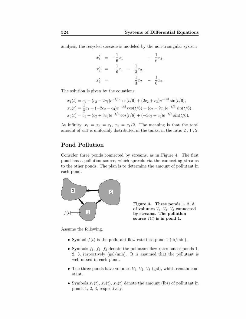
Consider three ponds connected by streams, as in Figure 4. The firstpond has a pollution source, which spreads via the connecting streamsto the other ponds. The plan is to determine the amount of pollutant ineach pond.

1

23

f(t)

Figure 4. Three ponds 1, 2, 3

of volumes V1, V2, V3 connected

by streams. The pollution

source f(t) is in pond 1.

Assume the following.

• Symbol f(t) is the pollutant flow rate into pond 1 (lb/min).

• Symbols f1, f2, f3 denote the pollutant flow rates out of ponds 1,2, 3, respectively (gal/min). It is assumed that the pollutant iswell-mixed in each pond.

• The three ponds have volumes V1, V2, V3 (gal), which remain con-stant.

• Symbols x1(t), x2(t), x3(t) denote the amount (lbs) of pollutant inponds 1, 2, 3, respectively.


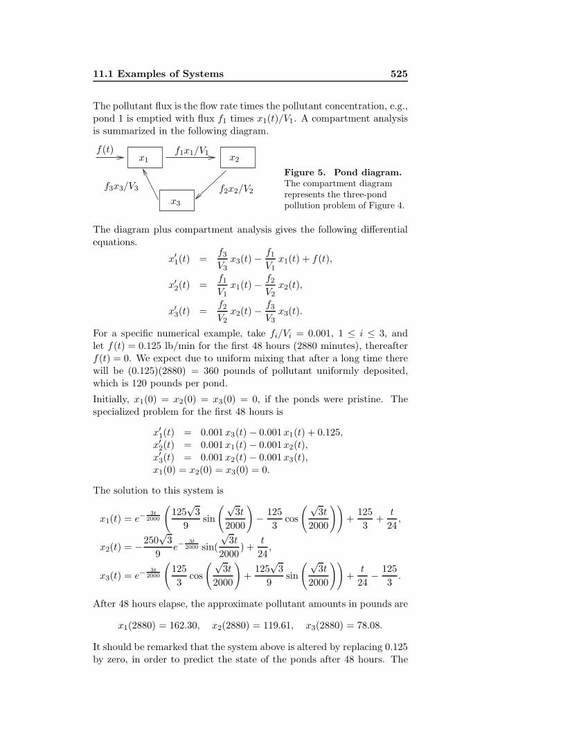
The pollutant flux is the flow rate times the pollutant concentration, e.g.,pond 1 is emptied with flux f1 times x1(t)/V1. A compartment analysisis summarized in the following diagram.

x2

x3

x1f1x1/V1f(t)

f3x3/V3 f2x2/V2

Figure 5. Pond diagram.

The compartment diagramrepresents the three-pondpollution problem of Figure 4.

The diagram plus compartment analysis gives the following differentialequations.

x′1(t) =

f3

V3x3(t)−

f1

V1x1(t) + f(t),

x′2(t) =

f1

V1x1(t)−

f2

V2x2(t),

x′3(t) =

f2

V2x2(t)−

f3

V3x3(t).

For a specific numerical example, take fi/Vi = 0.001, 1 ≤ i ≤ 3, andlet f(t) = 0.125 lb/min for the first 48 hours (2880 minutes), thereafterf(t) = 0. We expect due to uniform mixing that after a long time therewill be (0.125)(2880) = 360 pounds of pollutant uniformly deposited,which is 120 pounds per pond.

Initially, x1(0) = x2(0) = x3(0) = 0, if the ponds were pristine. Thespecialized problem for the first 48 hours is

x′1(t) = 0.001x3(t)− 0.001x1(t) + 0.125,

x′2(t) = 0.001x1(t)− 0.001x2(t),

x′3(t) = 0.001x2(t)− 0.001x3(t),

x1(0) = x2(0) = x3(0) = 0.

The solution to this system is

x1(t) = e−3t

2000

(

125√

3

9sin

( √3t

2000

)

− 125

3cos

( √3t

2000

))

+125

3+

t

24,

x2(t) = −250√

3

9e−

3t2000 sin(

√3t

2000) +

t

24,

x3(t) = e−3t

2000

(

125

3cos

( √3t

2000

)

+125√

3

9sin

( √3t

2000

))

+t

24− 125

3.

After 48 hours elapse, the approximate pollutant amounts in pounds are

x1(2880) = 162.30, x2(2880) = 119.61, x3(2880) = 78.08.

It should be remarked that the system above is altered by replacing 0.125by zero, in order to predict the state of the ponds after 48 hours. The


corresponding homogeneous system has an equilibrium solution x1(t) =x2(t) = x3(t) = 120. This constant solution is the limit at infinity ofthe solution to the homogeneous system, using the initial values x1(0) ≈162.30, x2(0) ≈ 119.61, x3(0) ≈ 78.08.

Home Heating

Consider a typical home with attic, basement and insulated main floor.

Attic

MainFloor

BasementFigure 6. Typical home

with attic and basement.

The below-grade basementand the attic are un-insulated.Only the main living area isinsulated.

It is usual to surround the main living area with insulation, but the atticarea has walls and ceiling without insulation. The walls and floor in thebasement are insulated by earth. The basement ceiling is insulated byair space in the joists, a layer of flooring on the main floor and a layerof drywall in the basement. We will analyze the changing temperaturesin the three levels using Newton’s cooling law and the variables

z(t) = Temperature in the attic,

y(t) = Temperature in the main living area,

x(t) = Temperature in the basement,

t = Time in hours.

Initial data. Assume it is winter time and the outside temperaturein constantly 35◦F during the day. Also assumed is a basement earthtemperature of 45◦F. Initially, the heat is off for several days. The initialvalues at noon (t = 0) are then x(0) = 45, y(0) = z(0) = 35.

Portable heater. A small electric heater is turned on at noon, withthermostat set for 100◦F. When the heater is running, it provides a 20◦Frise per hour, therefore it takes some time to reach 100◦F (probablynever!). Newton’s cooling law

Temperature rate = k(Temperature difference)

will be applied to five boundary surfaces: (0) the basement walls andfloor, (1) the basement ceiling, (2) the main floor walls, (3) the main


floor ceiling, and (4) the attic walls and ceiling. Newton’s cooling lawgives positive cooling constants k0, k1, k2, k3, k4 and the equations

x′ = k0(45− x) + k1(y − x),y′ = k1(x− y) + k2(35 − y) + k3(z − y) + 20,z′ = k3(y − z) + k4(35 − z).

The insulation constants will be defined as k0 = 1/2, k1 = 1/2, k2 = 1/4,k3 = 1/4, k4 = 1/2 to reflect insulation quality. The reciprocal 1/kis approximately the amount of time in hours required for 63% of thetemperature difference to be exchanged. For instance, 4 hours elapse forthe main floor. The model:

x′ =1

2(45 − x) +

1

2(y − x),

y′ =1

2(x− y) +

1

4(35 − y) +

1

4(z − y) + 20,

z′ =1

4(y − z) +

1

2(35− z).

The homogeneous solution in vector form is given in terms of constantsa = (7 −

√21)/8, b = (7 +

√21)/8, c = −1 +

√21, d = −1 −

√21 and

arbitrary constants c1, c2, c3 by the formula

xh(t)yh(t)zh(t)

= c1e

−t/2

122

+ c2e

−at

4c2

+ c3e

−bt

4d2

.

A particular solution is an equilibrium solution

xp(t)yp(t)zp(t)

=

4558

2754

1854

.

The homogeneous solution has limit zero at infinity, hence the temper-atures of the three spaces hover around x = 57, y = 69, z = 46 degreesFahrenheit. Specific information can be gathered by solving for c1, c2, c3

according to the initial data x(0) = 45, y(0) = z(0) = 35. The answersare

c1 = −85

24, c2 = −25

24− 115

√21

168, c3 = −25

24+

115√

21

168.

Underpowered heater. To the main floor each hour is added 20◦F, butthe heat escapes at a substantial rate, so that after one hour y ≈ 51◦F.After five hours, y ≈ 65◦F. The heater in this example is so inadequatethat even after many hours, the main living area is still under 69◦F.

Forced air furnace. Replacing the space heater by a normal furnaceadds the difficulty of switches in the input, namely, the thermostat


turns off the furnace when the main floor temperature reaches 70◦F,and it turns it on again after a 4◦F temperature drop. We will supposethat the furnace has four times the BTU rating of the space heater,which translates to an 80◦F temperature rise per hour. The study ofthe forced air furnace requires two differential equations, one with 20replaced by 80 (DE 1, furnace on) and the other with 20 replaced by 0(DE 2, furnace off). The plan is to use the first differential equation ontime interval 0 ≤ t ≤ t1, then switch to the second differential equationfor time interval t1 ≤ t ≤ t2. The time intervals are selected so thaty(t1) = 70 (the thermostat setting) and y(t2) = 66 (thermostat settingless 4 degrees). Numerical work gives the following results.

Time in minutes Main floor temperature Model Furnace

31.6 70 DE 1 on40.9 66 DE 2 off45.3 70 DE 1 on55.0 66 DE 2 off

The reason for the non-uniform times between furnace cycles can beseen from the model. Each time the furnace cycles, heat enters the mainfloor, then escapes through the other two levels. Consequently, the initialconditions applied to models 1 and 2 are changing, resulting in differentsolutions to the models on each switch.

Chemostats and Microorganism Culturing

A vessel into which nutrients are pumped, to feed a microorganism,is called a chemostat1. Uniform distributions of microorganisms andnutrients are assumed, for example, due to stirring effects. The pumpingis matched by draining to keep the volume constant.

In a typical chemostat, one nutrient is kept in short supply while allothers are abundant. We consider here the question of survival of theorganism subject to the limited resource. The problem is quantified asfollows:

x(t) = the concentration of the limited nutrient in the vessel,

y(t) = the concentration of organisms in the vessel.

1The October 14, 2004 issue of the journal Nature featured a study of the co-

evolution of a common type of bacteria, Escherichia coli, and a virus that infects

it, called bacteriophage T7. Postdoctoral researcher Samantha Forde set up ”micro-

bial communities of bacteria and viruses with different nutrient levels in a series of

chemostats – glass culture tubes that provide nutrients and oxygen and siphon off

wastes.”


A special case of the derivation in J.M. Cushing’s text for the organismE. Coli2 is the set of nonlinear differential equations

x′ = −0.075x + (0.075)(0.005) − 1

63g(x)y,

y′ = −0.075y + g(x)y,(2)

where g(x) = 0.68x(0.0016 + x)−1. Of special interest to the study ofthis equation are two linearized equations at equilibria, given by

u′1 = −0.075u1 − 0.008177008175u2 ,

u′2 = 0.4401515152u2 ,

(3)

v′1 = −1.690372243 v1 − 0.001190476190 v2 ,v′2 = 101.7684513 v1 .

(4)

Although we cannot solve the nonlinear system explicitly, neverthelessthere are explicit formulae for u1, u2, v1, v2 that complete the picture ofhow solutions x(t), y(t) behave at t = ∞. The result of the analysis isthat E. Coli survives indefinitely in this vessel at concentration y ≈ 0.3.

Irregular Heartbeats and Lidocaine

The human malady of ventricular arrhythmia or irregular heartbeatis treated clinically using the drug lidocaine.

Figure 7. Xylocaine label, a brand name for

the drug lidocaine.

To be effective, the drug has to be maintained at a bloodstream concen-tration of 1.5 milligrams per liter, but concentrations above 6 milligramsper liter are considered lethal in some patients. The actual dosage de-pends upon body weight. The adult dosage maximum for ventriculartachycardia is reported at 3 mg/kg.3 The drug is supplied in 0.5%, 1%and 2% solutions, which are stored at room temperature.

A differential equation model for the dynamics of the drug therapy uses

2In a biology Master’s thesis, two strains of Escherichia coli were grown in a glucose-

limited chemostat coupled to a modified Robbins device containing plugs of silicone

rubber urinary catheter material. Reference: Jennifer L. Adams and Robert J. C.

McLean, Applied and Environmental Microbiology, September 1999, p. 4285-4287,

Vol. 65, No. 9.3Source: Family Practice Notebook, http://www.fpnotebook.com/. The au-

thor is Scott Moses, MD, who practises in Lino Lakes, Minnesota.


x(t) = amount of lidocaine in the bloodstream,

y(t) = amount of lidocaine in body tissue.

A typical set of equations, valid for a special body weight only, appearsbelow; for more detail see J.M. Cushing’s text [?].

x′(t) = −0.09x(t) + 0.038y(t),y′(t) = 0.066x(t) − 0.038y(t).

(5)

The physically significant initial data is zero drug in the bloodstreamx(0) = 0 and injection dosage y(0) = y0. The answers:

x(t) = −0.3367y0e−0.1204t + 0.3367y0e

−0.0076t,

y(t) = 0.2696y0e−0.1204t + 0.7304y0e

−0.0076t.

The answers can be used to estimate the maximum possible safe dosagey0 and the duration of time that the drug lidocaine is effective.

Nutrient Flow in an Aquarium

Consider a vessel of water containing a radioactive isotope, to be used asa tracer for the food chain, which consists of aquatic plankton varietiesA and B.

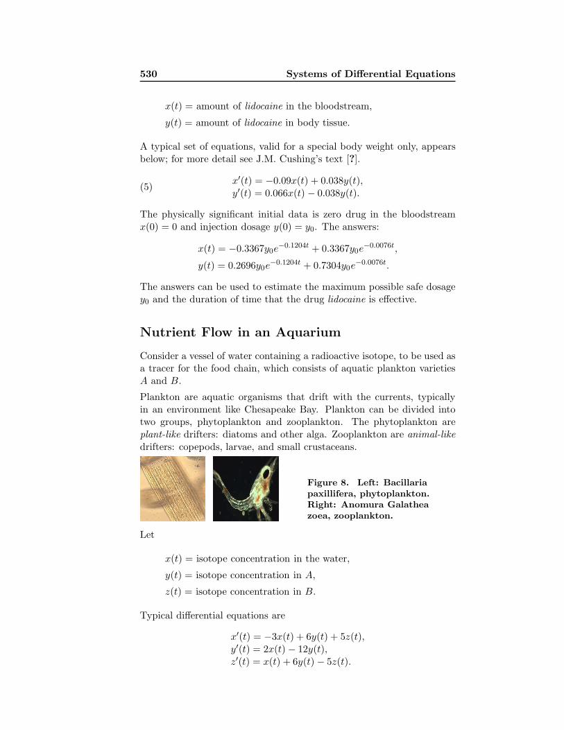
Plankton are aquatic organisms that drift with the currents, typicallyin an environment like Chesapeake Bay. Plankton can be divided intotwo groups, phytoplankton and zooplankton. The phytoplankton areplant-like drifters: diatoms and other alga. Zooplankton are animal-like

drifters: copepods, larvae, and small crustaceans.

Figure 8. Left: Bacillaria

paxillifera, phytoplankton.

Right: Anomura Galathea

zoea, zooplankton.

Let

x(t) = isotope concentration in the water,

y(t) = isotope concentration in A,

z(t) = isotope concentration in B.

Typical differential equations are

x′(t) = −3x(t) + 6y(t) + 5z(t),y′(t) = 2x(t) − 12y(t),z′(t) = x(t) + 6y(t) − 5z(t).


The answers are

x(t) = 6c1 + (1 +√

6)c2e(−10+

√6)t + (1−

√6)c3e

(−10−√

6)t,

y(t) = c1 + c2e(−10+

√6)t + c3e

(−10−√

6)t,

z(t) =12

5c1 −

(

2 +√

1.5)

c2e(−10+

√6)t +

(

−2 +√

1.5)

c3e(−10−

√6)t.

The constants c1, c2, c3 are related to the initial radioactive isotopeconcentrations x(0) = x0, y(0) = 0, z(0) = 0, by the 3 × 3 system oflinear algebraic equations

6c1 + (1 +√

6)c2 + (1−√

6)c3 = x0,c1 + c2 + c3 = 0,

12

5c1 −

(

2 +√

1.5)

c2 +(

−2 +√

1.5)

c3 = 0.

Biomass Transfer

Consider a European forest having one or two varieties of trees. Weselect some of the oldest trees, those expected to die off in the next fewyears, then follow the cycle of living trees into dead trees. The dead treeseventually decay and fall from seasonal and biological events. Finally,the fallen trees become humus. Let variables x, y, z, t be defined by

x(t) = biomass decayed into humus,

y(t) = biomass of dead trees,

z(t) = biomass of living trees,

t = time in decades (decade = 10 years).

A typical biological model is

x′(t) = −x(t) + 3y(t),y′(t) = −3y(t) + 5z(t),z′(t) = −5z(t).

Suppose there are no dead trees and no humus at t = 0, with initially z0

units of living tree biomass. These assumptions imply initial conditionsx(0) = y(0) = 0, z(0) = z0. The solution is

x(t) =15

8z0

(

e−5t − 2e−3t + e−t)

,

y(t) =5

2z0

(

−e−5t + e−3t)

,

z(t) = z0e−5t.

The live tree biomass z(t) = z0e−5t decreases according to a Malthusian

decay law from its initial size z0. It decays to 60% of its original biomass


in one year. Interesting calculations that can be made from the otherformulae include the future dates when the dead tree biomass and thehumus biomass are maximum. The predicted dates are approximately2.5 and 8 years hence, respectively.

The predictions made by this model are trends extrapolated from rateobservations in the forest. Like weather prediction, it is a calculatedguess that disappoints on a given day and from the outset has no pre-dictable answer.

Total biomass is considered an important parameter to assess atmo-spheric carbon that is harvested by trees. Biomass estimates for forestssince 1980 have been made by satellite remote sensing data with instancesof 90% accuracy (Science 87(5), September 2004).

Pesticides in Soil and Trees

A Washington cherry orchard was sprayed with pesticides.

Figure 9. Cherries in June.

Assume that a negligible amount of pesticide was sprayed on the soil.Pesticide applied to the trees has a certain outflow rate to the soil, andconversely, pesticide in the soil has a certain uptake rate into the trees.Repeated applications of the pesticide are required to control the insects,which implies the pesticide levels in the trees varies with time. Quantizethe pesticide spraying as follows.

x(t) = amount of pesticide in the trees,

y(t) = amount of pesticide in the soil,

r(t) = amount of pesticide applied to the trees,

t = time in years.

A typical model is obtained from input-output analysis, similar to thebrine tank models:

x′(t) = 2x(t)− y(t) + r(t),y′(t) = 2x(t)− 3y(t).

In a pristine orchard, the initial data is x(0) = 0, y(0) = 0, because thetrees and the soil initially harbor no pesticide. The solution of the model


obviously depends on r(t). The nonhomogeneous dependence is treatedby the method of variation of parameters infra. Approximate formulaeare

x(t) ≈∫ t

0

(

1.10e1.6(t−u) − 0.12e−2.6(t−u))

r(u)du,

y(t) ≈∫ t

0

(

0.49e1.6(t−u) − 0.49e−2.6(t−u))

r(u)du.

The exponential rates 1.6 and −2.6 represent respectively the accumu-lation of the pesticide into the soil and the decay of the pesticide fromthe trees. The application rate r(t) is typically a step function equal toa positive constant over a small interval of time and zero elsewhere, or asum of such functions, representing periodic applications of pesticide.

Forecasting Prices

A cosmetics manufacturer has a marketing policy based upon the pricex(t) of its salon shampoo.

Figure 10. Salon shampoo sample.

The marketing strategy for the shampoo is to set theprice x(t) dynamically to reflect demand for theproduct. A low inventory is desirable, to reduce theoverall cost of the product.

The production P (t) and the sales S(t) are given in terms of the price

x(t) and the change in price x′(t) by the equations

P (t) = 4− 3

4x(t)− 8x′(t) (Production),

S(t) = 15− 4x(t)− 2x′(t) (Sales).

The differential equations for the price x(t) and inventory level I(t) are

x′(t) = k(I(t)− I0),I ′(t) = P (t)− S(t).

The inventory level I0 = 50 represents the desired level. The equationscan be written in terms of x(t), I(t) as follows.

x′(t) = kI(t) − kI0,

I ′(t) =13

4x(t) − 6kI(t) + 6kI0 − 11.

If k = 1, x(0) = 10 and I(0) = 7, then the solution is given by

x(t) =44

13+

86

13e−13t/2,

I(t) = 50− 43e−13t/2.


The forecast of price x(t) ≈ 3.39 dollars at inventory level I(t) ≈ 50 isbased upon the two limits

limt→∞

x(t) =44

13, lim

t→∞I(t) = 50.

Coupled Spring-Mass Systems

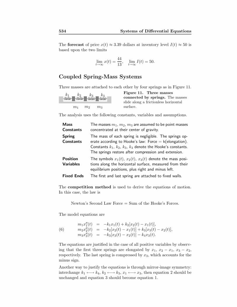
Three masses are attached to each other by four springs as in Figure 11.

m1 m3

k2 k3 k4k1

m2

Figure 11. Three masses

connected by springs. The massesslide along a frictionless horizontalsurface.

The analysis uses the following constants, variables and assumptions.

MassConstants

The masses m1, m2, m3 are assumed to be point massesconcentrated at their center of gravity.

SpringConstants

The mass of each spring is negligible. The springs op-erate according to Hooke’s law: Force = k(elongation).Constants k1, k2, k3, k4 denote the Hooke’s constants.The springs restore after compression and extension.

PositionVariables

The symbols x1(t), x2(t), x3(t) denote the mass posi-tions along the horizontal surface, measured from theirequilibrium positions, plus right and minus left.

Fixed Ends The first and last spring are attached to fixed walls.

The competition method is used to derive the equations of motion.In this case, the law is

Newton’s Second Law Force = Sum of the Hooke’s Forces.

The model equations are

m1x′′1(t) = −k1x1(t) + k2[x2(t)− x1(t)],

m2x′′2(t) = −k2[x2(t)− x1(t)] + k3[x3(t)− x2(t)],

m3x′′3(t) = −k3[x3(t)− x2(t)]− k4x3(t).

(6)

The equations are justified in the case of all positive variables by observ-ing that the first three springs are elongated by x1, x2 − x1, x3 − x2,respectively. The last spring is compressed by x3, which accounts for theminus sign.

Another way to justify the equations is through mirror-image symmetry:interchange k1 ←→ k4, k2 ←→ k3, x1 ←→ x3, then equation 2 should beunchanged and equation 3 should become equation 1.


Matrix Formulation. System (6) can be written as a second ordervector-matrix system

m1 0 00 m2 00 0 m3

x′′1

x′′2

x′′3

=

−k1 − k2 k2 0k2 −k2 − k3 k3

0 k3 −k3 − k4

x1

x2

x3

.

More succinctly, the system is written as

Mx′′(t) = Kx(t)

where the displacement x, mass matrix M and stiffness matrix Kare defined by the formulae

x=

x1

x2

x3

, M =

m1 0 00 m2 00 0 m3

, K =

−k1 − k2 k2 0k2 −k2 − k3 k3

0 k3 −k3 − k4

.

Numerical example. Let m1 = 1, m2 = 1, m3 = 1, k1 = 2, k2 = 1,k3 = 1, k4 = 2. Then the system is given by

x′′1

x′′2

x′′3

=

−3 1 01 −2 10 1 −3

x1

x2

x3

.

The vector solution is given by the formula

x1

x2

x3

= (a1 cos t + b1 sin t)

121

+(

a2 cos√

3t + b2 sin√

3t)

10−1

+ (a3 cos 2t + b3 sin 2t)

1−1

1

,

where a1, a2, a3, b1, b2, b3 are arbitrary constants.

Boxcars

A special case of the coupled spring-mass system is three boxcars on alevel track connected by springs, as in Figure 12.

k k

m mm

Figure 12. Three identical

boxcars connected by

identical springs.


Except for the springs on fixed ends, this problem is the same as the oneof the preceding illustration, therefore taking k1 = k4 = 0, k2 = k3 = k,m1 = m2 = m3 = m gives the system

m 0 00 m 00 0 m

x′′1

x′′2

x′′3

=

−k k 0k −2k k0 k −k

x1

x2

x3

.

Take k/m = 1 to obtain the illustration

x′′ =

−1 1 01 −2 10 1 −1

x,

which has vector solution

x = (a1 + b1t)

111

+ (a2 cos t + b2 sin t)

10−1

+(

a3 cos√

3t + b3 sin√

3t)

1−2

1

,

where a1, a2, a3, b1, b2, b3 are arbitrary constants.

The solution expression can be used to discover what happens to theboxcars when the springs act normally upon compression but disengageupon expansion. An interesting physical situation is when one car movesalong the track, contacts two stationary cars, then transfers its momen-tum to the other cars, followed by disengagement.

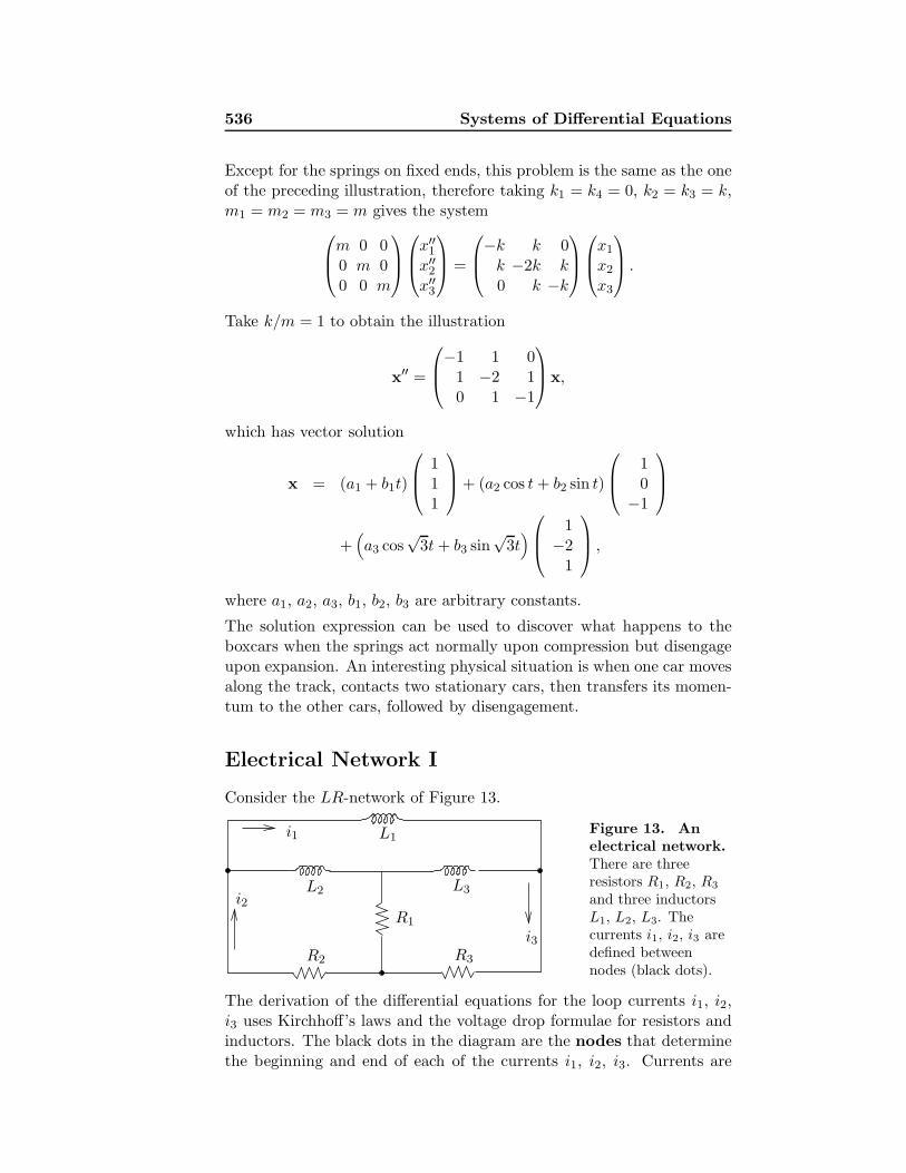
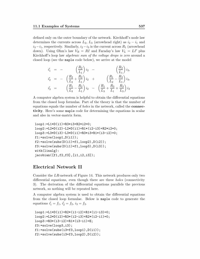
Electrical Network I

Consider the LR-network of Figure 13.

R1

i3R3R2

L3L2

L1i1

i2

Figure 13. An

electrical network.

There are threeresistors R1, R2, R3

and three inductorsL1, L2, L3. Thecurrents i1, i2, i3 aredefined betweennodes (black dots).

The derivation of the differential equations for the loop currents i1, i2,i3 uses Kirchhoff’s laws and the voltage drop formulae for resistors andinductors. The black dots in the diagram are the nodes that determinethe beginning and end of each of the currents i1, i2, i3. Currents are


defined only on the outer boundary of the network. Kirchhoff’s node lawdetermines the currents across L2, L3 (arrowhead right) as i2 − i1 andi3−i1, respectively. Similarly, i2−i3 is the current across R1 (arrowheaddown). Using Ohm’s law VR = RI and Faraday’s law VL = LI ′ plusKirchhoff’s loop law algebraic sum of the voltage drops is zero around aclosed loop (see the maple code below), we arrive at the model

i′1 = −(

R2

L1

)

i2 −(

R3

L1

)

i3,

i′2 = −(

R2

L2+

R2

L1

)

i2 +

(

R1

L2− R3

L1

)

i3,

i′3 =

(

R1

L3− R2

L1

)

i2 −(

R1

L3+

R3

L1+

R3

L3

)

i3

A computer algebra system is helpful to obtain the differential equationsfrom the closed loop formulas. Part of the theory is that the number ofequations equals the number of holes in the network, called the connec-

tivity. Here’s some maple code for determining the equations in scalarand also in vector-matrix form.

loop1:=L1*D(i1)+R3*i3+R2*i2=0;

loop2:=L2*D(i2)-L2*D(i1)+R1*(i2-i3)+R2*i2=0;

loop3:=L3*D(i3)-L3*D(i1)+R3*i3+R1*(i3-i2)=0;

f1:=solve(loop1,D(i1));

f2:=solve(subs(D(i1)=f1,loop2),D(i2));

f3:=solve(subs(D(i1)=f1,loop3),D(i3));

with(linalg):

jacobian([f1,f2,f3],[i1,i2,i3]);

Electrical Network II

Consider the LR-network of Figure 14. This network produces only twodifferential equations, even though there are three holes (connectivity3). The derivation of the differential equations parallels the previousnetwork, so nothing will be repeated here.

A computer algebra system is used to obtain the differential equationsfrom the closed loop formulae. Below is maple code to generate theequations i′1 = f1, i′2 = f2, i3 = f3.

loop1:=L1*D(i1)+R2*(i1-i2)+R1*(i1-i3)=0;

loop2:=L2*D(i2)+R3*(i2-i3)+R2*(i2-i1)=0;

loop3:=R3*(i3-i2)+R1*(i3-i1)=E;

f3:=solve(loop3,i3);

f1:=solve(subs(i3=f3,loop1),D(i1));

f2:=solve(subs(i3=f3,loop2),D(i2));


E

R1 R2

i1 L1

R3

i3 i2

L2

Figure 14. An electrical network.

There are three resistors R1, R2, R3, two inductors L1, L2 and a battery E.

The currents i1, i2, i3 are defined between nodes (black dots).

The model, in the special case L1 = L2 = 1 and R1 = R2 = R3 = R:

i′1 = − 3R

2i1 +

3R

2i2 +

E

2,

i′2 =3R

2i1 − 3R

2i2 +

E

2,

i3 =1

2i1 +

1

2i2 +

E

2R.

It is easily justified that the solution of the differential equations forinitial conditions i1(0) = i2(0) = 0 is given by

i1(t) =E

2t, i2(t) =

E

2t.

Logging Timber by Helicopter

Certain sections of National Forest in the USA do not have logging ac-cess roads. In order to log the timber in these areas, helicopters areemployed to move the felled trees to a nearby loading area, where theyare transported by truck to the mill. The felled trees are slung beneaththe helicopter on cables.

Figure 15. Helicopter logging.

Left: An Erickson helicopter lifts felledtrees.Right: Two trees are attached to thecable to lower transportation costs.

The payload for two trees approximates a double pendulum, which oscil-lates during flight. The angles of oscillation θ1, θ2 of the two connectingcables, measured from the gravity vector direction, satisfy the followingdifferential equations, in which g is the gravitation constant, m1, m2


denote the masses of the two trees and L1, L2 are the cable lengths.

(m1 + m2)L21θ

′′1 + m2L1L2θ

′′2 + (m1 + m2)L1gθ1 = 0,

m2L1L2θ′′1 + m2L

22θ

′′2 + m2L2gθ2 = 0.

This model is derived assuming small displacements θ1, θ2, that is,sin θ ≈ θ for both angles, using the following diagram.

θ2

L1

L2

m2

m1θ1

Figure 16. Logging Timber by Helicopter.

The cables have lengths L1, L2. The angles θ1, θ2 aremeasured from vertical.

The lengths L1, L2 are adjusted on each trip for the length of the trees,so that the trees do not collide in flight with each other nor with thehelicopter. Sometimes, three or more smaller trees are bundled togetherin a package, which is treated here as identical to a single, very thicktree hanging on the cable.

Vector-matrix model. The angles θ1, θ2 satisfy the second-ordervector-matrix equation

(

(m1 + m2)L1 m2L2

L1 L2

)(

θ1

θ2

)′′

= −(

m1g + m2g 00 g

)(

θ1

θ2

)

.

This system is equivalent to the second-order system

(

θ1

θ2

)′′

=

−m1g + m2g

L1m1

m2g

L1m1

m1g + m2 g

L2m1−(m1 + m2) g

L2m1

(

θ1

θ2

)

.

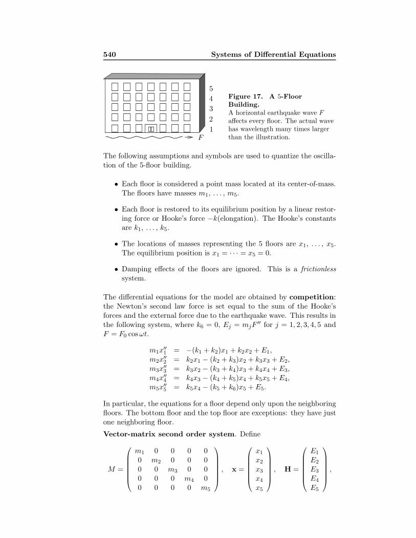
Earthquake Effects on Buildings

A horizontal earthquake oscillation F (t) = F0 cos ωt affects each floor ofa 5-floor building; see Figure 17. The effect of the earthquake dependsupon the natural frequencies of oscillation of the floors.

In the case of a single-floor building, the center-of-mass position x(t)of the building satisfies mx′′ + kx = E and the natural frequency ofoscillation is

√

k/m. The earthquake force E is given by Newton’s secondlaw: E(t) = −mF ′′(t). If ω ≈

√

k/m, then the amplitude of x(t) is largecompared to the amplitude of the force E. The amplitude increase inx(t) means that a small-amplitude earthquake wave can resonant withthe building and possibly demolish the structure.


3

F

4

5

1

2

Figure 17. A 5-Floor

Building.

A horizontal earthquake wave Faffects every floor. The actual wavehas wavelength many times largerthan the illustration.

The following assumptions and symbols are used to quantize the oscilla-tion of the 5-floor building.

• Each floor is considered a point mass located at its center-of-mass.The floors have masses m1, . . . , m5.

• Each floor is restored to its equilibrium position by a linear restor-ing force or Hooke’s force −k(elongation). The Hooke’s constantsare k1, . . . , k5.

• The locations of masses representing the 5 floors are x1, . . . , x5.The equilibrium position is x1 = · · · = x5 = 0.

• Damping effects of the floors are ignored. This is a frictionless

system.

The differential equations for the model are obtained by competition:the Newton’s second law force is set equal to the sum of the Hooke’sforces and the external force due to the earthquake wave. This results inthe following system, where k6 = 0, Ej = mjF

′′ for j = 1, 2, 3, 4, 5 andF = F0 cos ωt.

m1x′′1 = −(k1 + k2)x1 + k2x2 + E1,

m2x′′2 = k2x1 − (k2 + k3)x2 + k3x3 + E2,

m3x′′3 = k3x2 − (k3 + k4)x3 + k4x4 + E3,

m4x′′4 = k4x3 − (k4 + k5)x4 + k5x5 + E4,

m5x′′5 = k5x4 − (k5 + k6)x5 + E5.

In particular, the equations for a floor depend only upon the neighboringfloors. The bottom floor and the top floor are exceptions: they have justone neighboring floor.

Vector-matrix second order system. Define

M =

m1 0 0 0 00 m2 0 0 00 0 m3 0 00 0 0 m4 00 0 0 0 m5

, x =

x1

x2

x3

x4

x5

, H =

E1

E2

E3

E4

E5

,


K =

−k1 − k2 k2 0 0 0k2 −k2 − k3 k3 0 00 k3 −k3 − k4 k4 00 0 k4 −k4 − k5 k5

0 0 0 k5 −k5 − k6

.

In the last row, k6 = 0, to reflect the absence of a floor above the fifth.The second order system is

Mx′′(t) = Kx(t) + H(t).

The matrix M is called the mass matrix and the matrix K is called theHooke’s matrix. The external force H(t) can be written as a scalarfunction E(t) = −F ′′(t) times a constant vector:

H(t) = −ω2F0 cos ωt

m1

m2

m3

m4

m5

.

Identical floors. Let us assume that all floors have the same massm and the same Hooke’s constant k. Then M = mI and the equationbecomes

x′′ = m−1

−2k k 0 0 0k −2k k 0 00 k −2k k 00 0 k −2k k0 0 0 k −k

x− F0ω2 cos(ωt)

11111

.

The Hooke’s matrix K is symmetric (KT = K) with negative entriesonly on the diagonal. The last diagonal entry is −k (a common error isto write −2k).

Particular solution. The method of undetermined coefficients predictsa trial solution xp(t) = c cos ωt, because each differential equation hasnonhomogeneous term −F0ω

2 cos ωt. The constant vector c is foundby trial solution substitution. Cancel the common factor cos ωt in thesubstituted equation to obtain the equation

(

m−1K + ω2 I)

c = F0ω2b,

where b is column vector of ones in the preceding display. Let B(ω) =

m−1K + ω2 I. Then the formula B−1 =adj(B)

det(B)gives

c = F0ω2 adj(B(ω))

det(B(ω))b.

The constant vector c can have a large magnitude when det(B(ω)) ≈ 0.This occurs when −ω2 is nearly an eigenvalue of m−1K.


Homogeneous solution. The theory of this chapter gives the homo-geneous solution xh(t) as the sum

xh(t) =5∑

j=1

(aj cos ωjt + bj sin ωjt)vj

where r = ωj and v = vj 6= 0 satisfy

(

1

mK + r2 I

)

v = 0.

Special case k/m = 10. Then

1

mK =

−20 10 0 0 0

10 −20 10 0 0

0 10 −20 10 0

0 0 10 −20 10

0 0 0 10 −10

and the values ω1, . . . , ω5 are found by solving the determinant equationdet((1/m)K + ω2I) = 0, to obtain the values in Table 1.

Table 1. The natural frequencies for the special case k/m = 10.

Frequency Value

ω1 0.900078068ω2 2.627315231ω3 4.141702938ω4 5.320554507ω5 6.068366391

General solution. Superposition implies x(t) = xh(t) + xp(t). Bothterms of the general solution represent bounded oscillations.

Resonance effects. The special solution xp(t) can be used to obtainsome insight into practical resonance effects between the incoming earth-quake wave and the building floors. When ω is close to one of the fre-quencies ω1, . . . , ω5, then the amplitude of a component of xp can bevery large, causing the floor to take an excursion that is too large tomaintain the structural integrity of the floor.

The physical interpretation is that an earthquake wave of the properfrequency, having time duration sufficiently long, can demolish a floorand hence demolish the entire building. The amplitude of the earthquakewave does not have to be large: a fraction of a centimeter might beenough to start the oscillation of the floors.


The Richter Scale, Earthquakes and Tsunamis

The Richter scale was invented by C. Richter, a seismologist, to rateearthquake power. The Richter scale magnitude R of an earthquake is

R = log10

(

A

T

)

+ B

where A is the amplitude of the ground motion in microns at the receivingstation and T is the period in seconds of the seismic wave. The empiricalterm B = B(d) depends on the distance d from the epicenter to thereceiving station, e.g., B(6250) ≈ 6.8 where d is in miles. The period T isrelated to the natural frequency ω of the wave by the relation T = 2π/ω.A wave of period 2 seconds with A = 32 microns at receiving station6250 miles from the epicenter would have an earthquake magnitude of8.0 on the Richter scale. The highest reported magnitude is 9.6 on theRichter scale, for the Concepcion, Chile earthquake of May 22, 1960.

The Sumatra 9.0 earthquake of December 26, 2004 occurred close to adeep-sea trench, a subduction zone where one tectonic plate slips beneathanother. Most of the earthquake energy is released in these areas as thetwo plates grind towards each other.

The Chile earthquake and tsunami of 1960 has been documented well.Here is an account by Dr. Gerard Fryer of the Hawaii Institute of Geo-physics and Planetology, in Honolulu.

The tsunami was generated by the Chile earthquake of May 22,1960, the largest earthquake ever recorded: it was magnitude 9.6.What happened in the earthquake was that a piece of the Pacificseafloor (or strictly speaking, the Nazca Plate) about the size ofCalifornia slid fifty feet beneath the continent of South America.Like a spring, the lower slopes of the South American continentoffshore snapped upwards as much as twenty feet while land alongthe Chile coast dropped about ten feet. This change in the shape ofthe ocean bottom changed the shape of the sea surface. Since thesea surface likes to be flat, the pile of excess water at the surfacecollapsed to create a series of waves — the tsunami.

The tsunami, together with the coastal subsidence and flooding,caused tremendous damage along the Chile coast, where about2,000 people died. The waves spread outwards across the Pa-cific. About 15 hours later the waves flooded Hilo, on the islandof Hawaii, where they built up to 30 feet and caused 61 deathsalong the waterfront. Seven hours after that, 22 hours after theearthquake, the waves flooded the coastline of Japan where 10-footwaves caused 200 deaths. The waves also caused damage in theMarquesas, in Samoa, and in New Zealand. Tidal gauges through-out the Pacific measured anomalous oscillations for about threedays as the waves bounced from one side of the ocean to the other.


11.2 Basic First-order System Methods

Solving 2× 2 Systems

It is shown here that any constant linear system

u′ = Au, A =

(

a bc d

)

can be solved by one of the following elementary methods.

(a) The integrating factor method for y′ = p(x)y + q(x).

(b) The second order constant coefficient recipe.

Triangular A. Let’s assume b = 0, so that A is lower triangular. Theupper triangular case is handled similarly. Then u′ = Au has the scalarform

u′1 = au1,

u′2 = cu1 + du2.

The first differential equation is solved by the growth/decay recipe:

u1(t) = u0eat.

Then substitute the answer just found into the second differential equa-tion to give

u′2 = du2 + cu0e

at.

This is a linear first order equation of the form y′ = p(x)y + q(x), to besolved by the integrating factor method. Therefore, a triangular systemcan always be solved by the first order integrating factor method.

An illustration. Let us solve u′ = Au for the triangular matrix

A =

(

1 02 1

)

.

The first equation u′1 = u1 has solution u1 = c1e

t. The second equationbecomes

u′2 = 2c1e

t + u2,

which is a first order linear differential equation with solution u2 =(2c1t + c2)e

t. The general solution of u′ = Au in scalar form is

u1 = c1et, u2 = 2c1te

t + c2et.

The vector form of the general solution is

u(t) = c1

(

et

2tet

)

+ c2

(

0et

)

.

11.2 Basic First-order System Methods 545

The vector basis is the set

B =

{(

et

2tet

)

,

(

0et

)}

.

Non-Triangular A. In order that A be non-triangular, both b 6= 0and c 6= 0 must be satisfied. The scalar form of the system u′ = Au is

u′1 = au1 + bu2,

u′2 = cu1 + du2.

Theorem 1 (Solving Non-Triangular u′ = Au)Solutions u1, u2 of u′ = Au are linear combinations of the list of atomsobtained from the roots r of the quadratic equation

det(A− rI) = 0.

Proof: The method: differentiate the first equation, then use the equations toeliminate u2, u′

2. The result is a second order differential equation for u1. Thesame differential equation is satisfied also for u2. The details:

u′′

1 = au′

1 + bu′

2 Differentiate the first equation.

= au′

1 + bcu1 + bdu2 Use equation u′

2 = cu1 + du2.

= au′

1 + bcu1 + d(u′

1 − au1) Use equation u′

1 = au1 + bu2.

= (a + d)u′

1 + (bc− ad)u1 Second order equation for u1 found

The characteristic equation of u′′

1 − (a + d)u′

1 + (ad− bc)u1 = 0 is

r2 − (a + d)r + (bc− ad) = 0.

Finally, we show the expansion of det(A − rI) is the same characteristic poly-nomial:

det(A− rI) =

∣

∣

∣

∣

a− r bc d− r

∣

∣

∣

∣

= (a− r)(d − r)− bc= r2 − (a + d)r + ad− bc.

The proof is complete.

The reader can verify that the differential equation for u1 or u2 is exactly

u′′ − trace(A)u′ + det(A)u = 0.

Finding u1. Apply the second order recipe to solve for u1. This involveswriting a list L of atoms corresponding to the two roots of the charac-teristic equation r2 − (a + d)r + ad − bc = 0, followed by expressing u1

as a linear combination of the two atoms.

Finding u2. Isolate u2 in the first differential equation by division:

u2 =1

b(u′

1 − au1).


The two formulas for u1, u2 represent the general solution of the systemu′ = Au, when A is 2× 2.

An illustration. Let’s solve u′ = Au when

A =

(

1 22 1

)

.

The equation det(A− rI) = 0 is (1− r)2 − 4 = 0 with roots r = −1 andr = 3. The atom list is L = {e−t, e3t}. Then the linear combination ofatoms is u1 = c1e

−t + c2e3t. The first equation u′

1 = u1 + 2u2 impliesu2 = 1

2(u′1 − u1). The general solution of u′ = Au is then

u1 = c1e−t + c2e

3t, u2 = −c1e−t + c2e

3t.

In vector form, the general solution is

u = c1

(

e−t

−e−t

)

+ c2

(

e3t

e3t

)

.

Triangular Methods

Diagonal n×n matrix A = diag(a1, . . . , an). Then the system x′ = Ax

is a set of uncoupled scalar growth/decay equations:

x′1(t) = a1x1(t),

x′2(t) = a2x2(t),

...x′

n(t) = anxn(t).

The solution to the system is given by the formulae

x1(t) = c1ea1t,

x2(t) = c2ea2t,

...xn(t) = cneant.

The numbers c1, . . . , cn are arbitrary constants.

Triangular n × n matrix A. If a linear system x′ = Ax has a squaretriangular matrix A, then the system can be solved by first order scalarmethods. To illustrate the ideas, consider the 3× 3 linear system

x′ =

2 0 03 3 04 4 4

x.


The coefficient matrix A is lower triangular. In scalar form, the systemis given by the equations

x′1(t) = 2x1(t),

x′2(t) = 3x1(t) + 3x2(t),

x′3(t) = 4x1(t) + 4x2(t) + 4x3(t).

A recursive method. The system is solved recursively by first orderscalar methods only, starting with the first equation x′

1(t) = 2x1(t). Thisgrowth equation has general solution x1(t) = c1e

2t. The second equationthen becomes the first order linear equation

x′2(t) = 3x1(t) + 3x2(t)

= 3x2(t) + 3c1e2t.

The integrating factor method applies to find the general solution x2(t) =−3c1e

2t+c2e3t. The third and last equation becomes the first order linear

equation

x′3(t) = 4x1(t) + 4x2(t) + 4x3(t)

= 4x3(t) + 4c1e2t + 4(−3c1e

2t + c2e3t).

The integrating factor method is repeated to find the general solutionx3(t) = 4c1e

2t − 4c2e3t + c3e

4t.

In summary, the solution to the system is given by the formulae

x1(t) = c1e2t,

x2(t) = −3c1e2t + c2e

3t,x3(t) = 4c1e

2t − 4c2e3t + c3e

4t.

Structure of solutions. A system x′ = Ax for n × n triangular Ahas component solutions x1(t), . . . , xn(t) given as polynomials timesexponentials. The exponential factors ea11t, . . . , eannt are expressed interms of the diagonal elements a11, . . . , ann of the matrix A. Fewer thann distinct exponential factors may appear, due to duplicate diagonalelements. These duplications cause the polynomial factors to appear.The reader is invited to work out the solution to the system below,which has duplicate diagonal entries a11 = a22 = a33 = 2.

x′1(t) = 2x1(t),

x′2(t) = 3x1(t) + 2x2(t),

x′3(t) = 4x1(t) + 4x2(t) + 2x3(t).

The solution, given below, has polynomial factors t and t2, appearingbecause of the duplicate diagonal entries 2, 2, 2, and only one exponentialfactor e2t.

x1(t) = c1e2t,

x2(t) = 3c1te2t + c2e

2t,x3(t) = 4c1te

2t + 6c1t2e2t + 4c2te

2t + c3e2t.


Conversion to Systems

Routinely converted to a system of equations of first order are scalarsecond order linear differential equations, systems of scalar second orderlinear differential equations and scalar linear differential equations ofhigher order.

Scalar second order linear equations. Consider an equationau′′ + bu′ + cu = f where a 6= 0, b, c, f are allowed to depend on t,′ = d/dt. Define the position-velocity substitution

x(t) = u(t), y(t) = u′(t).

Then x′ = u′ = y and y′ = u′′ = (−bu′− cu+f)/a = −(b/a)y− (c/a)x+f/a. The resulting system is equivalent to the second order equation, inthe sense that the position-velocity substitution equates solutions of onesystem to the other:

x′(t) = y(t),

y′(t) = − c(t)

a(t)x(t)− b(t)

a(t)y(t) +

f(t)

a(t).

The case of constant coefficients and f a function of t arises often enoughto isolate the result for further reference.

Theorem 2 (System Equivalent to Second Order Linear)Let a 6= 0, b, c be constants and f(t) continuous. Then au′′+bu′+cu = f(t)is equivalent to the first order system

aw′(t) =

(

0 a−c −b

)

w(t) +

(

0f(t)

)

, w(t) =

(

u(t)u′(t)

)

.

Converting second order systems to first order systems. A sim-ilar position-velocity substitution can be carried out on a system of twosecond order linear differential equations. Assume

a1u′′1 + b1u

′1 + c1u1 = f1,

a2u′′2 + b2u

′2 + c2u2 = f2.

Then the preceding methods for the scalar case give the equivalence

a1 0 0 00 a1 0 00 0 a2 00 0 0 a2

u1

u′1

u2

u′2

′

=

0 a1 0 0−c1 −b1 0 00 0 0 a2

0 0 −c2 −b2

u1

u′1

u2

u′2

+

0f1

0f2

.

Coupled spring-mass systems. Springs connecting undamped cou-pled masses were considered at the beginning of this chapter, page 534.


Typical equations are

m1x′′1(t) = −k1x1(t) + k2[x2(t)− x1(t)],

m2x′′2(t) = −k2[x2(t)− x1(t)] + k3[x3(t)− x2(t)],

m3x′′3(t) = −k3[x3(t)− x2(t)]− k4x3(t).

(1)

The equations can be represented by a second order linear system ofdimension 3 of the form Mx′′ = Kx, where the position x, the mass

matrix M and the Hooke’s matrix K are given by the equalities

x =

x1

x2

x3

, M =

m1 0 00 m2 00 0 m3

,

K =

−(k1 + k2) k2 0k2 −(k2 + k3) k3

0 −k3 −(k3 + k4)

.

Systems of second order linear equations. A second order sys-tem Mx′′ = Kx + F(t) is called a forced system and F is called theexternal vector force. Such a system can always be converted to a sec-ond order system where the mass matrix is the identity, by multiplyingby M−1:

x′′ = M−1Kx + M−1F(t).

The benign form x′′ = Ax + G(t), where A = M−1K and G = M−1F,admits a block matrix conversion into a first order system:

d

dt

(

x(t)x′(t)

)

=

(

0 I

A 0

)(

x(t)x′(t)

)

+

(

0

G(t)

)

.

Damped second order systems. The addition of a dampener to eachof the masses gives a damped second order system with forcing

Mx′′ = Bx′ + KX + F(t).

In the case of one scalar equation, the matrices M , B, K are constantsm, −c, −k and the external force is a scalar function f(t), hence thesystem becomes the classical damped spring-mass equation

mx′′ + cx′ + kx = f(t).

A useful way to write the first order system is to introduce variableu = Mx, in order to obtain the two equations

u′ = Mx′, u′′ = Bx′ + Kx + F(t).


Then a first order system in block matrix form is given by

(

M 0

0 M

)

d

dt

(

x(t)x′(t)

)

=

(

0 M

K B

)(

x(t)x′(t)

)

+

(

0

F(t)

)

.

The benign form x′′ = M−1Bx′ +M−1Kx+M−1F(t), obtained by left-multiplication by M−1, can be similarly written as a first order systemin block matrix form.

d

dt

(

x(t)x′(t)

)

=

(

0 I

M−1K M−1B

)(

x(t)x′(t)

)

+

(

0

M−1F(t)

)

.

Higher order linear equations. Every homogeneous nth orderconstant-coefficient linear differential equation

y(n) = p0y + · · ·+ pn−1y(n−1)

can be converted to a linear homogeneous vector-matrix system

d

dx

yy′

y′′

...

y(n−1)

=

0 1 0 · · · 00 0 1 · · · 0

...0 0 0 · · · 1p0 p1 p2 · · · pn−1

yy′

y′′

...

y(n−1)

.

This is a linear system u′ = Au where u is the n × 1 column vectorconsisting of y and its successive derivatives, while the n × n matrix Ais the classical companion matrix of the characteristic polynomial

rn = p0 + p1r + p2r2 + · · ·+ pn−1r

n−1.

To illustrate, the companion matrix for r4 = a + br + cr2 + dr3 is

A =

0 1 0 00 0 1 00 0 0 1a b c d

.

The preceding companion matrix has the following block matrix form,which is representative of all companion matrices.

A =

(

0 I

a b c d

)

.

Continuous coefficients. It is routinely observed that the methodsabove for conversion to a first order system apply equally as well tohigher order linear differential equations with continuous coefficients. To


illustrate, the fourth order linear equation yiv = a(x)y+b(x)y′+c(x)y′′+d(x)y′′′ has first order system form u′ = Au where A is the companionmatrix for the polynomial r4 = a(x) + b(x)r + c(x)r2 + d(x)r3, x heldfixed.

Forced higher order linear equations. All that has been said aboveapplies equally to a forced linear equation like

yiv = 2y + sin(x)y′ + cos(x)y′′ + x2y′′′ + f(x).

It has a conversion to a first order nonhomogeneous linear system

u′ =

0 1 0 00 0 1 00 0 0 12 sin x cos x x2

u +

000

f(x)

, u =

yy′

y′′

y′′′

.


11.3 Structure of Linear Systems

Linear systems. A linear system is a system of differential equa-tions of the form

x′1 = a11x1 + · · · + a1nxn + f1,

x′2 = a21x1 + · · · + a2nxn + f2,

...... · · · ...

...x′

m = am1x1 + · · · + amnxn + fm,

(1)

where ′ = d/dt. Given are the functions aij(t) and fj(t) on some intervala < t < b. The unknowns are the functions x1(t), . . . , xn(t).

The system is called homogeneous if all fj = 0, otherwise it is callednon-homogeneous.

Matrix Notation for Systems. A non-homogeneous system oflinear equations (1) is written as the equivalent vector-matrix system

x′ = A(t)x + f(t),

where

x =

x1...

xn

, f =

f1...

fn

, A =

a11 · · · a1n... · · · ...

am1 · · · amn

.

Existence-uniqueness. The fundamental theorem of Picard andLindelof applied to the matrix system x′ = A(t)x + f(t) says that aunique solution x(t) exists for each initial value problem and the solu-tion exists on the common interval of continuity of the entries in A(t)and f(t).

Three special results are isolated here, to illustrate how the Picard theoryis applied to linear systems.

Theorem 3 (Unique Zero Solution)Let A(t) be an m× n matrix with entries continuous on a < t < b. Thenthe initial value problem

x′ = A(t)x, x(0) = 0

has unique solution x(t) = 0 on a < t < b.

Theorem 4 (Existence-Uniqueness for Constant Linear Systems)Let A(t) = A be an m× n matrix with constant entries and let x0 be anym-vector. Then the initial value problem

x′ = Ax, x(0) = x0

has a unique solution x(t) defined for all values of t.

11.3 Structure of Linear Systems 553

Theorem 5 (Uniqueness and Solution Crossings)Let A(t) be an m × n matrix with entries continuous on a < t < b andassume f(t) is also continuous on a < t < b. If x(t) and y(t) are solutions ofu′ = A(t)u + f(t) on a < t < b and x(t0) = y(t0) for some t0, a < t0 < b,then x(t) = y(t) for a < t < b.

Superposition. Linear homogeneous systems have linear structure

and the solutions to nonhomogeneous systems obey a principle of su-

perposition.

Theorem 6 (Linear Structure)Let x′ = A(t)x have two solutions x1(t), x2(t). If k1, k2 are constants,then x(t) = k1 x1(t) + k2 x2(t) is also a solution of x′ = A(t)x.

The standard basis {wk}nk=1. The Picard-Lindelof theorem appliedto initial conditions x(t0) = x0, with x0 successively set equal to thecolumns of the n × n identity matrix, produces n solutions w1, . . . ,wn to the equation x′ = A(t)x, all of which exist on the same intervala < t < b.

The linear structure theorem implies that for any choice of the constantsc1, . . . , cn, the vector linear combination

x(t) = c1w1(t) + c2w2(t) + · · · + cnwn(t)(2)

is a solution of x′ = A(t)x.

Conversely, if c1, . . . , cn are taken to be the components of a given vectorx0, then the above linear combination must be the unique solution ofthe initial value problem with x(t0) = x0. Therefore, all solutions of theequation x′ = A(t)x are given by the expression above, where c1, . . . , cn

are taken to be arbitrary constants. In summary:

Theorem 7 (Basis)The solution set of x′ = A(t)x is an n-dimensional subspace of the vectorspace of all vector-valued functions x(t). Every solution has a unique basisexpansion (2).

Theorem 8 (Superposition Principle)Let x′ = A(t)x+f(t) have a particular solution xp(t). If x(t) is any solutionof x′ = A(t)x + f(t), then x(t) can be decomposed as homogeneous plusparticular:

x(t) = xh(t) + xp(t).

The term xh(t) is a certain solution of the homogeneous differential equationx′ = A(t)x, which means arbitrary constants c1, c2, . . . have been assignedcertain values. The particular solution xp(t) can be selected to be free ofany unresolved or arbitrary constants.


Theorem 9 (Difference of Solutions)Let x′ = A(t)x + f(t) have two solutions x = u(t) and x = v(t). Definey(t) = u(t)− v(t). Then y(t) satisfies the homogeneous equation

y′ = A(t)y.

General Solution. We explain general solution by example. If aformula x = c1e

t + c2e2t is called a general solution, then it means that

all possible solutions of the differential equation are expressed by thisformula. In particular, it means that a given solution can be representedby the formula, by specializing values for the constants c1, c2. We expectthe number of arbitrary constants to be the least possible number.

The general solution of x′ = A(t)x+ f(t) is an expression involving arbi-trary constants c1, c2, . . . and certain functions. The expression is oftengiven in vector notation, although scalar expressions are commonplaceand perfectly acceptable. Required is that the expression represents allsolutions of the differential equation, in the following sense:

(a) Every assignment of constants produces a solution ofthe differential equation.

(b) Every possible solution is uniquely obtained from theexpression by specializing the constants.

Due to the superposition principle, the constants in the general solutionare identified as multipliers against solutions of the homogeneous differ-ential equation. The general solution has some recognizable structure.

Theorem 10 (General Solution)Let A(t) be n×n and f(t) n×1, both continuous on an interval a < t < b.The linear nonhomogeneous system x′ = A(t)x + f(t) has general solutionx given by the expression

x = xh(t) + xp(t).

The term y = xh(t) is a general solution of the homogeneous equationy′ = A(t)y, in which are to be found n arbitrary constants c1, . . . , cn. Theterm x = xp(t) is a particular solution of x′ = A(t)x + f(t), in which thereare present no unresolved nor arbitrary constants.

Recognition of homogeneous solution terms. An expression x

for the general solution of a nonhomogeneous equation x′ = A(t)x+ f(t)involves arbitrary constants c1, . . . , cn. It is possible to isolate bothterms xh and xp by a simple procedure.

To find xp, set to zero all arbitrary constants c1, c2, . . . ; the resultingexpression is free of unresolved and arbitrary constants.


To find xh, we find first the vector solutions y = uk(t) of y′ = A(t)y,which are multiplied by constants ck. Then the general solution xh ofthe homogeneous equation y′ = A(t)y is given by

xh(t) = c1u1(t) + c2u2(t) + · · · + cnun(t).

Use partial derivatives on expression x to find the column vectors

uk(t) =∂

∂ckx.

This technique isolates the vector components of the homogeneous solu-tion from any form of the general solution, including scalar formulas forthe components of x. In any case, the general solution x of the linearsystem x′ = A(t)x + f(t) is represented by the expression

x = c1u1(t) + c2u2(t) + · · · + cnun(t) + xp(t).

In this expression, each assignment of the constants c1, . . . , cn producesa solution of the nonhomogeneous system, and conversely, each possiblesolution of the nonhomogeneous system is obtained by a unique special-

ization of the constants c1, . . . , cn.

To illustrate the ideas, consider a 3 × 3 linear system x′ = A(t)x + f(t)with general solution

x =

x1

x2

x3

given in scalar form by the expressions

x1 = c1et + c2e

−t + t,x2 = (c1 + c2)e

t + c3e2t,

x3 = (2c2 − c1)e−t + (4c1 − 2c3)e

2t + 2t.

To find the vector form of the general solution, we take partial derivatives

uk =∂x

∂ckwith respect to the variable names c1, c2, c3:

u1 =

et

et

−e−t + 4e2t

, u2 =

e−t

et

2e−t

, u3 =

0e2t

−2e2t

.

To find xp(t), set c1 = c2 = c3 = 0:

xp(t) =

t0

2t

.


Finally,

x = c1u1(t) + c2u2(t) + c3u3(t) + xp(t)

= c1

et

et

−e−t + 4e2t

+ c2

e−t

et

2e−t

+ c3

0e2t

−2e2t

+

t0

2t

.

The expression x = c1u1(t) + c2u2(t) + c3u3(t) + xp(t) satisfies requiredelements (a) and (b) in the definition of general solution. We will developnow a way to routinely test the uniqueness requirement in (b).

Independence. Constants c1, . . . , cn in the general solution x =xh + xp appear exactly in the expression xh, which has the form

xh = c1u1 + c2u2 + · · · + cnun.

A solution x uniquely determines the constants. In particular, the zerosolution of the homogeneous equation is uniquely represented, which canbe stated this way:

c1u1 + c2u2 + · · ·+ cnun = 0 implies c1 = c2 = · · · = cn = 0.

This statement is equivalent to the statement that the vector-valuedfunctions u1(t), . . . , un(t) are linearly independent.

It is possible to write down a candidate general solution to some 3 × 3linear system x′ = Ax via equations like

x1 = c1et + c2e

t + c3e2t,

x2 = c1et + c2e

t + 2c3e2t,

x3 = c1et + c2e

t + 4c3e2t.

This example was constructed to contain a classic mistake, for purposesof illustration.

How can we detect a mistake, given only that this expression is supposedto represent the general solution? First of all, we can test that u1 =∂x/∂c1, u2 = ∂x/∂c2, u3 = ∂x/∂c3 are indeed solutions. But to insurethe unique representation requirement, the vector functions u1, u2, u3

must be linearly independent. We compute

u1 =

et

et

et

, u2 =

et

et

et

, u3 =

e2t

2e2t

4e2t

.

Therefore, u1 = u2, which implies that the functions u1, u2, u3 fail to beindependent. While is is possible to test independence by a rudimentarytest based upon the definition, we prefer the following test due to Abel.


Theorem 11 (Abel’s Formula and the Wronskian)Let xh(t) = c1u1(t) + · · ·+ cnun(t) be a candidate general solution to theequation x′ = A(t)x. In particular, the vector functions u1(t), . . . , un(t)are solutions of x′ = A(t)x. Define the Wronskian by

w(t) = det(aug(u1(t), . . . ,un(t))).

Then Abel’s formula holds:

w(t) = e

∫ t

t0trace(A(s))ds

w(t0).4

In particular, w(t) is either everywhere nonzero or everywhere zero, accord-ingly as w(t0) 6= 0 or w(t0) = 0.

Theorem 12 (Abel’s Wronskian Test for Independence)The vector solutions u1, . . . , un of x′ = A(t)x are independent if and onlyif the Wronskian w(t) is nonzero for some t = t0.

Clever use of the point t0 in Abel’s Wronskian test can lead to succinctindependence tests. For instance, let

u1 =

et

et

et

, u2 =

et

et

et

, u3 =

e2t

2e2t

4e2t

.

Then w(t) might appear to be complicated, but w(0) is obviously zerobecause it has two duplicate columns. Therefore, Abel’s Wronskian testdetects dependence of u1, u2, u3.

To illustrate Abel’s Wronskian test when it detects independence, con-sider the column vectors

u1 =

et

et

−e−t + 4e2t

, u2 =

e−t

et

2e−t

, u3 =

0e2t

−2e2t

.

At t = t0 = 0, they become the column vectors

u1 =

113

, u2 =

112

, u3 =

01−2

.

Then w(0) = det(aug(u1(0),u2(0),u3(0))) = 1 is nonzero, testing in-

dependence of u1, u2, u3.

4The trace of a square matrix is the sum of its diagonal elements. In literature,

the formula is called the Abel-Liouville formula.


Initial value problems and the rref method. An initial value

problem is the problem of solving for x, given

x′ = A(t)x + f(t), x(t0) = x0.

If a general solution is known,

x = c1u1(t) + · · · + cnun(t) + xp(t),

then the problem of finding x reduces to finding c1, . . . , cn in the relation

c1u1(t0) + · · ·+ cnun(t0) + xp(t0) = x0.

This is a matrix equation for the unknown constants c1, . . . , cn of theform Bc = d, where

B = aug(u1(t0), . . . ,un(t0)), c =

c1...cn

, d = x0 − xp(t0).

The rref -method applies to find c. The method is to perform swap,combination and multiply operations to C = aug(B,d) until rref(C) =aug(I, c).

To illustrate the method, consider the general solution

x1 = c1et + c2e

−t + t,x2 = (c1 + c2)e

t + c3e2t,

x3 = (2c2 − c1)e−t + (4c1 − 2c3)e

2t + 2t.

We shall solve for c1, c2, c3, given the initial condition x1(0) = 1, x2(0) =0, x3(0) = −1. The above relations evaluated at t = 0 give the system

1 = c1e0 + c2e

0 + 0,0 = (c1 + c2)e

0 + c3e0,

−1 = (2c2 − c1)e0 + (4c1 − 2c3)e

0 + 0.

In standard scalar form, this is the 3× 3 linear system

c1 + c2 = 1,c1 + c2 + c3 = 0,

3c1 + 2c2 − 2c3 = −1.

The augmented matrix C, to be reduced to rref form, is given by

C =

1 1 0 11 1 1 03 2 −2 −1

.


After the rref process is completed, we obtain

rref(C) =

1 0 0 −50 1 0 60 0 1 −1

.

From this display, we read off the answer c1 = −5, c2 = 6, c3 = −1 andreport the final answer

x1 = −5et + 6e−t + t,x2 = et − e2t,x3 = 17e−t − 18e2t + 2t.

Equilibria. An equilibrium point x0 of a linear system x′ = A(t)x isa constant solution, x(t) = x0 for all t. Mostly, this makes sense whenA(t) is constant, although the definition applies to continuous systems.For a solution x to be constant means x′ = 0, hence all equilibria aredetermined from the equation

A(t)x0 = 0 for all t.

This is a homogeneous system of linear algebraic equations to be solvedfor x0. It is not allowed for the answer x0 to depend on t (if it does, thenit is not an equilibrium). The theory for a constant matrix A(t) ≡ Asays that either x0 = 0 is the unique solution or else there are infinitelymany answers for x0 (the nullity of A is positive).


11.4 Matrix Exponential

The problem

x′(t) = Ax(t), x(0) = x0

has a unique solution, according to the Picard-Lindelof theorem. Solvethe problem n times, when x0 equals a column of the identity matrix,and write w1(t), . . . , wn(t) for the n solutions so obtained. Define thematrix exponential by packaging these n solutions into a matrix:

eAt ≡ aug(w1(t), . . . ,wn(t)).

By construction, any possible solution of x′ = Ax can be uniquely ex-pressed in terms of the matrix exponential eAt by the formula

x(t) = eAtx(0).

Matrix Exponential Identities

Announced here and proved below are various formulae and identitiesfor the matrix exponential eAt:

(

eAt)′

= AeAt Columns satisfy x′ = Ax.

e0 = I Where 0 is the zero matrix.

BeAt = eAtB If AB = BA.

eAteBt = e(A+B)t If AB = BA.

eAteAs = eA(t+s) At and As commute.(

eAt)−1

= e−At Equivalently, eAte−At = I.

eAt = r1(t)P1 + · · · + rn(t)Pn Putzer’s spectral formula —see page 563.

eAt = eλ1tI +eλ1t − eλ2t

λ1 − λ2(A− λ1I) A is 2× 2, λ1 6= λ2 real.

eAt = eλ1tI + teλ1t(A− λ1I) A is 2× 2, λ1 = λ2 real.

eAt = eat cos bt I +eat sin bt

b(A− aI) A is 2×2, λ1 = λ2 = a+ ib,

b > 0.

eAt =∞∑

n=0

An tn

n!Picard series. See page 565.

eAt = P−1eJtP Jordan form J = PAP−1.

11.4 Matrix Exponential 561

Putzer’s Spectral Formula

The spectral formula of Putzer applies to a system x′ = Ax to find thegeneral solution, using matrices P1, . . . , Pn constructed from A and theeigenvalues λ1, . . . , λn of A, matrix multiplication, and the solution r(t)of the first order n× n initial value problem

r′(t) =

λ1 0 0 · · · 0 01 λ2 0 · · · 0 00 1 λ3 · · · 0 0

...0 0 0 · · · 1 λn

r(t), r(0) =

10...0

.

The system is solved by first order scalar methods and back-substitution.We will derive the formula separately for the 2 × 2 case (the one usedmost often) and the n× n case.

Putzer’s 2× 2 Spectral Formula

The general solution of x′ = Ax is given by the formula

x(t) = (r1(t)P1 + r2(t)P2)x(0),

where r1, r2, P1, P2 are defined as follows.

The eigenvalues r = λ1, λ2 are the two roots of the quadratic equation

det(A− rI) = 0.

Define 2× 2 matrices P1, P2 by the formulae

P1 = I, P2 = A− λ1I.

The functions r1(t), r2(t) are defined by the differential system

r′1 = λ1r1, r1(0) = 1,r′2 = λ2r2 + r1, r2(0) = 0.

Proof: The Cayley-Hamilton formula (A − λ1I)(A − λ2I) = 0 is valid forany 2 × 2 matrix A and the two roots r = λ1, λ2 of the determinant equalitydet(A− rI) = 0. The Cayley-Hamilton formula is the same as (A− λ2)P2 = 0,which implies the identity AP2 = λ2P2. Compute as follows.

x′(t) = (r′1(t)P1 + r′2(t)P2)x(0)

= (λ1r1(t)P1 + r1(t)P2 + λ2r2(t)P2)x(0)

= (r1(t)A + λ2r2(t)P2)x(0)

= (r1(t)A + r2(t)AP2)x(0)

= A (r1(t)I + r2(t)P2)x(0)

= Ax(t).

This proves that x(t) is a solution. Because Φ(t) ≡ r1(t)P1 + r2(t)P2 satisfiesΦ(0) = I, then any possible solution of x′ = Ax can be represented by the givenformula. The proof is complete.


Real Distinct Eigenvalues. Suppose A is 2×2 having real distincteigenvalues λ1, λ2 and x(0) is real. Then

r1 = eλ1t, r2 =eλ1t − eλ2T

λ1 − λ2

and

x(t) =

(

eλ1tI +eλ1t − eλ2t

λ1 − λ2(A− λ1I)

)

x(0).

The matrix exponential formula for real distinct eigenvalues:

eAt = eλ1tI +eλ1t − eλ2t

λ1 − λ2(A− λ1I).

Real Equal Eigenvalues. Suppose A is 2 × 2 having real equaleigenvalues λ1 = λ2 and x(0) is real. Then r1 = eλ1t, r2 = teλ1t and

x(t) =(

eλ1tI + teλ1t(A− λ1I))

x(0).

The matrix exponential formula for real equal eigenvalues:

eAt = eλ1tI + teλ1t(A− λ1I).

Complex Eigenvalues. Suppose A is 2 × 2 having complex eigen-values λ1 = a + bi with b > 0 and λ2 = a − bi. If x(0) is real, then areal solution is obtained by taking the real part of the spectral formula.This formula is formally identical to the case of real distinct eigenvalues.Then

Re(x(t)) = (Re(r1(t))I +Re(r2(t)(A− λ1I)))x(0)

=

(

Re(e(a+ib)t)I +Re(eat sin bt

b(A− (a + ib)I))

)

x(0)

=

(

eat cos bt I + eat sin bt

b(A− aI))

)

x(0)

The matrix exponential formula for complex conjugate eigenvalues:

eAt = eat(

cos bt I +sin bt

b(A− aI))

)

.

How to Remember Putzer’s 2× 2 Formula. The expressions

eAt = r1(t)I + r2(t)(A− λ1I),

r1(t) = eλ1t, r2(t) =eλ1t − eλ2t

λ1 − λ2

(1)

are enough to generate all three formulae. The fraction r2(t) is a differ-ence quotient with limit teλ1t as λ2 → λ1, therefore the formula includes


the case λ1 = λ2 by limiting. If λ1 = λ2 = a + ib with b > 0, then thefraction r2 is already real, because it has for z = eλ1t and w = λ1 theform

r2(t) =z − z

w −w=

sin bt

b.

Taking real parts of expression (1) then gives the complex case formulafor eAt.

Putzer’s n× n Spectral Formula

The general solution of x′ = Ax is given by the formula

x(t) = (r1(t)P1 + r2(t)P2 + · · ·+ rn(t)Pn)x(0),

where r1, r2, . . . , rn, P1, P2, . . . , Pn are defined as follows.

The eigenvalues r = λ1, . . . , λn are the roots of the polynomial equation

det(A− rI) = 0.

Define n× n matrices P1, . . . , Pn by the formulae

P1 = I, Pk = Pk−1(A− λk−1I), k = 2, . . . , n.

More succinctly, Pk = Πk−1j=1(A−λjI). The functions r1(t), . . . , rn(t) are

defined by the differential system

r′1 = λ1r1, r1(0) = 1,r′2 = λ2r2 + r1, r2(0) = 0,

...r′n = λnrn + rn−1, rn(0) = 0.

Proof: The Cayley-Hamilton formula (A − λ1I) · · · (A − λnI) = 0 is valid forany n× n matrix A and the n roots r = λ1, . . . , λn of the determinant equalitydet(A − rI) = 0. Two facts will be used: (1) The Cayley-Hamilton formulaimplies APn = λnPn; (2) The definition of Pk implies λkPk + Pk+1 = APk for1 ≤ k ≤ n− 1. Compute as follows.

1 x′(t) = (r′1(t)P1 + · · ·+ r′n(t)Pn)x(0)

2 =

(

n∑

k=1

λkrk(t)Pk +

n∑

k=2

rk−1Pk

)

x(0)

3 =

(

n−1∑

k=1

λkrk(t)Pk + rn(t)λnPn +

n−1∑

k=1

rkPk+1

)

x(0)

4 =

(

n−1∑

k=1

rk(t)(λkPk + Pk+1) + rn(t)λnPn

)

x(0)


5 =

(

n−1∑

k=1

rk(t)APk + rn(t)APn

)

x(0)

6 = A

(

n∑

k=1

rk(t)Pk

)

x(0)

7 = Ax(t).

Details: 1 Differentiate the formula for x(t). 2 Use the differential equa-

tions for r1,. . . ,rn. 3 Split off the last term from the first sum, then re-index

the last sum. 4 Combine the two sums. 5 Use the recursion for Pk and

the Cayley-Hamilton formula (A − λnI)Pn = 0. 6 Factor out A on the left.

7 Apply the definition of x(t).

This proves that x(t) is a solution. Because Φ(t) ≡ ∑n

k=1 rk(t)Pk satisfiesΦ(0) = I, then any possible solution of x′ = Ax can be so represented. Theproof is complete.

Proofs of Matrix Exponential Properties

Verify(

eAt)′

= AeAt. Let x0 denote a column of the identity matrix. Define

x(t) = eAtx0. Then(

eAt)

′

x0 = x′(t)= Ax(t)= AeAtx0.

Because this identity holds for all columns of the identity matrix, then (eAt)′ and

AeAt have identical columns, hence we have proved the identity(

eAt)

′

= AeAt.

Verify AB = BA implies BeAt = eAtB. Define w1(t) = eAtBw0 andw2(t) = BeAtw0. Calculate w′

1(t) = Aw1(t) and w′

2(t) = BAeAtw0 =ABeAtw0 = Aw2(t), due to BA = AB. Because w1(0) = w2(0) = w0, then theuniqueness assertion of the Picard-Lindelof theorem implies that w1(t) = w2(t).Because w0 is any vector, then eAtB = BeAt. The proof is complete.

Verify eAteBt = e(A+B)t. Let x0 be a column of the identity matrix. Definex(t) = eAteBtx0 and y(t) = e(A+B)tx0. We must show that x(t) = y(t) forall t. Define u(t) = eBtx0. We will apply the result eAtB = BeAt, valid forBA = AB. The details:

x′(t) =(

eAtu(t))

′

= AeAtu(t) + eAtu′(t)= Ax(t) + eAtBu(t)= Ax(t) + BeAtu(t)= (A + B)x(t).

We also know that y′(t) = (A + B)y(t) and since x(0) = y(0) = x0, then thePicard-Lindelof theorem implies that x(t) = y(t) for all t. This completes theproof.


Verify eAteAs = eA(t+s). Let t be a variable and consider s fixed. Definex(t) = eAteAsx0 and y(t) = eA(t+s)x0. Then x(0) = y(0) and both satisfy thedifferential equation u′(t) = Au(t). By the uniqueness in the Picard-Lindeloftheorem, x(t) = y(t), which implies eAteAs = eA(t+s). The proof is complete.

Verify eAt =∞∑

n=0

An tn

n!. The idea of the proof is to apply Picard iteration.

By definition, the columns of eAt are vector solutions w1(t), . . . , wn(t) whosevalues at t = 0 are the corresponding columns of the n × n identity matrix.According to the theory of Picard iterates, a particular iterate is defined by

yn+1(t) = y0 +

∫ t

0

Ayn(r)dr, n ≥ 0.

The vector y0 equals some column of the identity matrix. The Picard iteratescan be found explicitly, as follows.

y1(t) = y0 +∫ t

0 Ay0dr= (I + At)y0,

y2(t) = y0 +∫ t

0Ay1(r)dr

= y0 +∫ t

0A (I + At)y0dr

=(

I + At + A2t2/2)

y0,...

yn(t) =(

I + At + A2 t2

2 + · · ·+ An tn

n!

)

y0.

The Picard-Lindelof theorem implies that for y0 = column k of the identitymatrix,

limn→∞

yn(t) = wk(t).

This being valid for each index k, then the columns of the matrix sum

N∑

m=0

Am tm

m!

converge as N →∞ to w1(t), . . . , wn(t). This implies the matrix identity

eAt =∞∑

n=0

An tn

n!.

The proof is complete.

Theorem 13 (Special Formulas for eAt)

ediag(λ1,...,λn)t = diag(

eλ1t, . . . , eλnt)

Real or complex constantsλ1, . . . , λn.

e

(

a b−b a

)

t

= eat

(

cos bt sin bt− sin bt cos bt

)

Real a, b.


Theorem 14 (Computing eJt for J Triangular)If J is an upper triangular matrix, then a column u(t) of eJt can be computedby solving the system u′(t) = Ju(t), u(0) = v, where v is the correspond-ing column of the identity matrix. This problem can always be solved byfirst-order scalar methods of growth-decay theory and the integrating factormethod.

Theorem 15 (Block Diagonal Matrix)If A = diag(B1, . . . , Bk) and each of B1, . . . , Bk is a square matrix, then

eAt = diag(

eB1t, . . . , eBkt)

.

11.5 The Eigenanalysis Method 567

11.5 The Eigenanalysis Method

The general solution x(t) = eAtx(0) of the linear system

x′ = Ax

can be obtained entirely by eigenanalysis of the matrix A. A compu-tationally useful case is when the n × n matrix A has n independenteigenvectors in its list of eigenpairs

(λ1,v1), (λ2,v2), . . . , (λn,vn).

It is not required that the eigenvalues λ1, . . . , λn be distinct. Theeigenvalues can be real or complex.

The Eigenanalysis Method for a 2× 2 Matrix

Suppose that A is 2× 2 real and has eigenpairs

(λ1,v1), (λ2,v2),

with v1, v2 independent. The eigenvalues λ1, λ2 can be both real. Also,they can be a complex conjugate pair λ1 = λ2 = a + ib with b > 0.

It will be shown that the general solution of x′ = Ax can be written as

x(t) = c1eλ1tv1 + c2e

λ2tv2.

The details:

x′ = c1(eλ1t)′v1 + c2(e

λ2t)′v2 Differentiate the formula for x.

= c1eλ1tλ1v1 + c2e

λ2tλ2v2

= c1eλ1tAv1 + c2e

λ2tAv2 Use λ1v1 = Av1, λ2v2 = Av2.

= A(

c1eλ1tv1 + c2e

λ2tv2

)

Factor A left.

= Ax Definition of x.

Let’s rewrite the solution x in the vector-matrix form

x(t) = aug(v1,v2)

(

eλ1t 00 eλ2t

)(

c1

c2

)

.

Because eigenvectors v1, v2 are assumed independent, then aug(v1,v2)is invertible and setting t = 0 in the previous display gives

(

c1

c2

)

= aug(v1,v2)−1x(0).


Because c1, c2 can be chosen to produce any initial condition x(0), thenx(t) is the general solution of the system x′ = Ax.

The general solution expressed as x(t) = eAtx(0) leads to the exponentialmatrix relation

eAt = aug(v1,v2)

(

eλ1t 00 eλ2t

)

aug(v1,v2)−1.

The formula is immediately useful when the eigenpairs are real.

Complex conjugate eigenvalues. First, eigenpair (λ2,v2) is nevercomputed or used, because Av1 = λ1v1 implies Av1 = λ1v1, whichimplies λ2 = λ1 has eigenvector v2 = v1.

If A is real, then eAt is real, and taking real parts across the formula foreAt will give a real formula. Due to the unpleasantness of the complexalgebra, we will report the answer found, which is real, and then justifyit with minimal use of complex numbers.

Define for eigenpair (λ1,v1) symbols a, b, P as follows:

λ1 = a + ib, b > 0, P = aug(Re(v1),Im(v1)).

Then

eAt = eatP

(


)

P−1.(1)

Justification of (1). The formula is established by showing that the matrixΦ(t) on the right satisfies Φ(0) = I and Φ′ = AΦ. Then by definition, eAt =Φ(t). For exposition, let

R(t) = eat

(


)

, Φ(t) = PR(t)P−1.

The identity Φ(0) = I verified as follows.

Φ(0) = PR(0)P−1

= Pe0IP−1

= I

The expansion of eigenpair relation

A (Re(v1) + i Im(v1)) = (a + ib) (Re(v1) + i Im(v1))

into real and imaginary parts shows that

AP = P

(

a b−b a

)

.

ThenΦ′(t)Φ−1(t) = PR′(t)P−1PR−1(t)P−1

= PR′(t)R−1(t)P−1

= P

(

aI +

(

0 b−b 0

))

P−1

= P

(

a b−b a

)

P−1

= A


The proof of Φ′(t) = AΦ(t) is complete.

The formula for eAt implies that the general solution in this special caseis

x(t) = eat aug(Re(v1),Im(v1))

(


)(

c1

c2

)

.

The values c1, c2 are related to the initial condition x(0) by the matrixidentity

(

c1

c2

)

= aug(Re(v1),Im(v1))−1x(0).

The Eigenanalysis Method for a 3× 3 Matrix

Suppose that A is 3× 3 real and has eigenpairs

(λ1,v1), (λ2,v2), (λ3,v3),

with v1, v2, v3 independent. The eigenvalues λ1, λ2, λ3 can be all real.Also, there can be one real eigenvalue λ3 and a complex conjugate pairof eigenvalues λ1 = λ2 = a + ib with b > 0.

The general solution of x′ = Ax can be written as

x(t) = c1eλ1tv1 + c2e

λ2tv2 + c3eλ3tv3.

The details parallel the 2× 2 details; they are left as an exercise for thereader.

The solution x is written in vector-matrix form

x(t) = aug(v1,v2,v3)

eλ1t 0 00 eλ2t 00 0 eλ3t

c1

c2

c3

.

Because the three eigenvectors v1, v2, v3 are assumed independent, thenaug(v1,v2,v3) is invertible. Setting t = 0 in the previous display gives

c1

c2

c2

= aug(v1,v2,v3)

−1x(0).

Constants c1, c2, c3 can be chosen to produce any initial condition x(0),therefore x(t) is the general solution of the 3× 3 system x′ = Ax. Thereis a corresponding exponential matrix relation

eAt = aug(v1,v2,v3)

eλ1t 0 00 eλ2t 00 0 eλ3t

aug(v1,v2,v3)

−1.


This formula is normally used when the eigenpairs are real. When thereis a complex conjugate pair of eigenvalues λ1 = λ2 = a + ib, b > 0, thenas was shown in the 2 × 2 case it is possible to extract a real solutionx from the complex formula and report a real form for the exponentialmatrix:

eAt = P

eat cos bt eat sin bt 0−eat sin bt eat cos bt 0

0 0 eλ3t

P−1,

P = aug(Re(v1),Im(v1),v3).

The Eigenanalysis Method for an n× n Matrix

The general solution formula and the formula for eAt generalize easilyfrom the 2× 2 and 3× 3 cases to the general case of an n× n matrix.

Theorem 16 (The Eigenanalysis Method)Let the n× n real matrix A have eigenpairs

(λ1,v1), (λ2,v2), . . . , (λn,vn),

with n independent eigenvectors v1, . . . , vn. Then the general solution ofthe linear system x′ = Ax is given by

x(t) = c1v1eλ1t + c2v2e

λ2t + · · ·+ cnvneλnt.

The vector-matrix form of the general solution is

x(t) = aug(v1, . . . ,vn)diag(eλ1t, . . . , eλnt)

c1...

cn

.

This form is real provided all eigenvalues are real. A real form can bemade from a complex form by following the example of a 3 × 3 matrixA. The plan is to list all complex eigenvalues first, in pairs, λ1, λ1, . . . ,λp, λp. Then the real eigenvalues r1, . . . , rq are listed, 2p+ q = n. Define

P = aug(Re(v1),Im(v1), . . . ,Re(v2p−1),Im(v2p−1),v2p+1, . . . ,vn),

Rλ(t) = eat

(


)

, where λ + a + ib, b > 0.

Then the real vector-matrix form of the general solution is

x(t) = P diag(Rλ1(t), . . . , Rλp

(t), er1t, . . . , erqt)

c1...cn

andeAt = P diag(Rλ1

(t), . . . , Rλp(t), er1t, . . . , erqt)P−1.


Spectral Theory Methods

The simplicity of Putzer’s spectral method for computing eAt is appre-ciated, but we also recognize that the literature has an algorithm tocompute eAt, devoid of differential equations, which is of fundamentalimportance in linear algebra. The parallel algorithm computes eAt di-rectly from the eigenvalues λj of A and certain products of the nilpotentmatrices A−λjI. Called spectral formulae, they can be implementedin a numerical laboratory or computer algebra system, in order to effi-ciently compute eAt, even in the case of multiple eigenvalues.

Theorem 17 (Computing eAt for Simple Eigenvalues)Let the n × n matrix A have n simple eigenvalues λ1, . . . , λn (possiblycomplex) and define constant matrices Q1, . . . , Qn by the formulas

Qj = Πi6=jA− λiI

λj − λi, j = 1, . . . , n.

Then

eAt = eλ1tQ1 + · · · + eλntQn.

Theorem 18 (Computing eAt for Multiple Eigenvalues)Let the n× n matrix A have k distinct eigenvalues λ1, . . . , λk of algebraicmultiplicities m1, . . . , mk. Let p(λ) = det(A− λI) and define polynomialsa1(λ), . . . , ak(λ) by the partial fraction identity

1

p(λ)=

a1(λ)

(λ− λ1)m1

+ · · ·+ ak(λ)

(λ− λk)mk.

Define constant matrices Q1, . . . , Qk by the formulas

Qj = aj(A)Πi6=j(A− λiI)mi , j = 1, . . . , k.

Then

eAt =k∑

i=1

eλit Qi

mi−1∑

j=0

(A− λiI)jtj

j!.(2)

Proof: Let Ni = Qi(A− λiI), 1 ≤ i ≤ k. We first prove

Lemma 1 (Properties)1. Q1 + · · ·+ Qk = I,2. QiQi = Qi,3. QiQj = 0 for i 6= j,4. NiNj = 0 for i 6= j,5. Nmi

i = 0,

6. A =∑k

i=1(λiQi + Ni).


The proof of 1 follows from clearing fractions in the partial fraction expansionof 1/p(λ):

1 =

k∑

i=1

ai(λ)p(λ)

(λ − λi)mi.

The projection property 2 follows by multiplication of identity 1 by Qi andthen using 2.

The proof of 3 starts by observing that Qi and Qj together contain all thefactors of p(A), therefore QiQj = q(A)p(A) for some polynomial q. The Cayley-Hamilton theorem p(A) = 0 finishes the proof.

To prove 4, write NiNj = (A− λiI)(A− λjI)QiQj and apply 3.

To prove 5, use Qmi

i = Qi (from 2) to write Nmi

i = (A−λiI)miQi = p(A) = 0.

To prove 6, multiply 1 by A and rearrange as follows:

A =∑k

i=1 AQi

=∑k

i=1 λiQi + (A− λiI)Qi

=∑k

i=1 λiQi + Ni

To prove (2), multiply 1 by eAt and compute as follows:

eAt =∑k

i=1 QieAt

=∑k

i=1 QieλiIt+(A−λiI)t

=∑k

i=1 Qieλite(A−λiI)t

=∑k

i=1 QieλiteQi(A−λiI)t

=∑k

i=1 QieλiteNit

=∑k

i=1 Qieλit∑m1−1

j=0 (A− λiI)j tj

j!

Solving Planar Systems x′(t) = Ax(t)

A 2× 2 real system x′(t) = Ax(t) can be solved in terms of the roots ofthe characteristic equation det(A− λI) = 0 and the real matrix A.

Theorem 19 (Planar System, Putzer’s Spectral Recipe)Consider the real planar system x′(t) = Ax(t). Let λ1, λ2 be the roots ofthe characteristic equation det(A− λI) = 0. The real general solution x(t)is given by the formula

x(t) = eAtx(0)

where the 2× 2 exponential matrix eAt is given as follows.

Real λ1 6= λ2 eAt = eλ1tI +eλ2t − eλ1t

λ2 − λ1(A− λ1I).

Real λ1 = λ2 eAt = eλ1tI + teλ1t(A− λ1I).

Complex λ1 = λ2,λ1 = a + bi, b > 0

eAt = eat cos bt I +eat sin(bt)

b(A− aI).


Proof: The formulae are from Putzer’s algorithm, or equivalently, from thespectral formulae, with rearranged terms. The complex case is formally thereal part of the distinct root case when λ2 = λ1. The spectral recipe is theanalog of the recipe for second order equations with constant coefficients.

Illustrations. Typical cases are represented by the following 2 × 2matrices A, which correspond to roots λ1, λ2 of the characteristic equa-tion det(A − λI) = 0 which are real distinct, real double or complexconjugate. The solution x(t) = eAtx(0) is given here in two forms, bywriting eAt using 1 a spectral formula and 2 Putzer’s spectral

recipe.

λ1 = 5, λ2 = 2

A =

(

−1 3−6 8

)

Real distinct roots.

1 eAt =e5t

3

(

−3 3−6 6

)

+e2t

−3

(

−6 3−6 3

)

2 eAt = e5tI +e2t − e5t

2− 5

(

−6 3−6 3

)

λ1 = λ2 = 3

A =

(

2 1−1 4

)

Real double root.

1 eAt = e3t

(

I + t

(

−1 1−1 1

))

2 eAt = e3tI + te3t

(

−1 1−1 1

)

λ1 = λ2 = 2 + 3i

A =

(

2 3−3 2

)

Complex conjugate roots.

1 eAt = 2Re

(

e2t+3it

2(3i)

(

3i 3−3 3i

))

2 eAt = e2t cos 3tI +e2t sin 3t

3

(

0 3−3 0

)

The complex example is typical for real n×n matrices A with a complexconjugate pair of eigenvalues λ1 = λ2. Then Q2 = Q1. The result isthat λ2 is not used and we write instead a simpler expression using thecollege algebra equality z + z = 2Re(z):

eλ1tQ1 + eλ2tQ2 = 2Re(

eλ1tQ1

)

.

This observation explains why eAt is real when A is real, by pairingcomplex conjugate eigenvalues in the spectral formula.


11.6 Jordan Form and Eigenanalysis

Generalized Eigenanalysis

The main result of generalized eigenanalysis is Jordan’s theorem

A = PJP−1,

valid for any real or complex square matrix A. We describe here howto compute the invertible matrix P of generalized eigenvectors and theupper triangular matrix J , called a Jordan form of A:

J =

λ1 J12 0 · · · 0 0...

......

......

...0 0 0 · · · λn−1 Jn−1 n

0 0 0 · · · 0 λn

.

Entries Ji i+1 of J along its super-diagonal are either 0 or 1, while diag-onal entries λi are eigenvalues of A. A Jordan form is therefore a band

matrix with nonzero entries only on its diagonal and super-diagonal.

The geometric multiplicity GeoMult(λ) is the nullity of A−λI, whichis the number of basis vectors in a solution to (A − λI)x = 0, or,equivalently, the number of free variables. The algebraic multiplic-

ity AlgMult(λ) is the largest integer k such that (r − λ)k divides thecharacteristic polynomial det(A− rI).

Theorem 20 (Algebraic and Geometric Multiplicity)Let A be a square real or complex matrix. then

1 ≤ GeoMult(λ) ≤ AlgMult(λ).(1)

In addition, there are the following relationships between the Jordan form Jand algebraic and geometric multiplicities.

GeoMult(λ) Equals the number of Jordan blocks B(λ,m) that ap-pear in J ,

AlgMult(λ) Equals the number of times λ is repeated along thediagonal of J .

Decoding the equation A = PJP−1. The relation A = PJP−1,equivalent to AP = PJ , can be expressed in terms of the columns of thematrix P . If J is a single Jordan block B(λ,m), then the columns v1,. . . , vm of P satisfy

Av1 = λv1,Av2 = λv2 + v1,

......

...Avm = λvm + vm−1.

11.6 Jordan Form and Eigenanalysis 575

Chains of generalized eigenvectors. Given an eigenvalue λ ofthe matrix A, the topic of generalized eigenanalysis determines a Jordanblock B(λ,m) in J by finding an m-chain of generalized eigenvectorsv1, . . . , vm, which appear as columns of P in the relation A = PJP−1.The very first vector v1 of the chain is an eigenvector, (A− λI)v1 = 0.The others v2, . . . , vk are not eigenvectors but satisfy

(A− λI)v2 = v1, . . . , (A− λI)vm = vm−1.

Implied by the term m-chain is insolvability of (A − λI)x = vm. Thechain size m is subject to the inequality 1 ≤ m ≤ AlgMult(λ).

The Jordan form J may contain several Jordan blocks for one eigenvalueλ. To illustrate, if J has only one eigenvalue λ and AlgMult(λ) = 3,then J might be constructed as follows:

J = diag(B(λ, 1), B(λ, 1), B(λ, 1)) or J =

λ 0 00 λ 00 0 λ

,

J = diag(B(λ, 1), B(λ, 2)) or J =

λ 0 00 λ 10 0 λ

,

J = B(λ, 3) or J =

λ 1 00 λ 10 0 λ

.

The three generalized eigenvectors for this example correspond to

J =

λ 0 00 λ 00 0 λ

↔ Three 1-chains,

J =

λ 0 00 λ 10 0 λ

↔ One 1-chain and one 2-chain,

J =

λ 1 00 λ 10 0 λ

↔ One 3-chain.

Computing m-chains. Let us fix the discussion to an eigenvalue λof A. Define N = A− λI and p = AlgMult(λ).

To compute an m-chain, start with an eigenvector v1 and solve recur-sively by rref methods Nvj+1 = vj until there fails to be a solution.This must seemingly be done for all possible choices of v1! The search form-chains terminates when p independent generalized eigenvectors havebeen calculated.


If A has an essentially unique eigenpair (λ,v1), then this process termi-nates immediately with an m-chain where m = p. The chain producesone Jordan block B(λ,m) and the generalized eigenvectors v1, . . . , vm

are recorded into the matrix P .

If u1, u2 form a basis for the eigenvectors of A corresponding to λ, thenthe problem Nx = 0 has 2 free variables. Therefore, we seek to find anm1-chain and an m2-chain such that m1 +m2 = p, corresponding to twoJordan blocks B(λ,m1) and B(λ,m2).

To understand the logic applied here, the reader should verify that forN = diag(B(0,m1), B(0,m2), . . . , B(0,mk)) the problem Nx = 0 hask free variables, because N is already in rref form. These remarksimply that a k-dimensional basis of eigenvectors of A for eigenvalue λcauses a search for mi-chains, 1 ≤ i ≤ k, such that m1 + · · · + mk = p,corresponding to k Jordan blocks B(λ,m1), . . . , B(λ,mk).

A common naive approach for computing generalized eigenvectors canbe illustrated by letting

A =

1 1 10 1 00 0 1

, u1 =

1−1

1

, u2 =

01−1

.

Matrix A has one eigenvalue λ = 1 and two eigenpairs (1,u1), (1,u2).Starting a chain calculation with v1 equal to either u1 or u2 gives a1-chain. This naive approach leads to only two independent generalizedeigenvectors. However, the calculation must proceed until three inde-pendent generalized eigenvectors have been computed. To resolve thetrouble, keep a 1-chain, say the one generated by u1, and start a newchain calculation using v1 = a1u1 + a2u2. Adjust the values of a1, a2

until a 2-chain has been computed:

aug(A− λI,v1) =

0 1 1 a1

0 0 0 −a1 + a2

0 0 0 a1 − a2

≈

0 1 1 a1

0 0 0 00 0 0 0

,

provided a1−a2 = 0. Choose a1 = a2 = 1 to make v1 = u1 +u2 6= 0 and

solve for v2 =(

0, 1, 0)

. Then u1 is a 1-chain and v1, v2 is a 2-chain.

The generalized eigenvectors u1, v1, v2 are independent and form thecolumns of P while J = diag(B(λ, 1), B(λ, 2)) (recall λ = 1). We justifyA = PJP−1 by testing AP = PJ , using the formulas

J =

λ 0 00 λ 10 0 λ

, P =

1 1 0−1 0 1

1 0 0

.


Jordan blocks

An m × m matrix B(λ,m) is called a Jordan block provided it is aJordan form, all m diagonal elements are the same eigenvalue λ and allsuper-diagonal elements are one:

B(λ,m) =

λ 1 0 · · · 0 0...

......

......

...0 0 0 · · · λ 10 0 0 · · · 0 λ

(m×m matrix)

The Jordan block form of J. Given a square matrix A, a Jordanform J for A is built from Jordan blocks, more precisely,

J = diag(B(λ1,m1), B(λ2,m2), . . . , B(λk,mk)),

where λ1, . . . , λk are eigenvalues of A and m1 + · · ·+mk = n. The k− 1zeros on the super-diagonal of J result from adjacent Jordan blocks. Forexample, no super-diagonal zeros means there is just one Jordan block.A complete specification of how to build J from A is done in generalized

eigenanalysis.

Theorem 21 (Exponential of a Jordan Block Matrix)If λ is real and

B =

λ 1 0 · · · 0 0...

......

......

...0 0 0 · · · λ 10 0 0 · · · 0 λ

(m×m matrix)

then

eBt = eλt

1 t t2

2 · · · tm−2

(m−2)!tm−1

(m−1)!...

......

......

...0 0 0 · · · 1 t0 0 0 · · · 0 1

.

The equality also holds if λ is a complex number, in which case both sidesof the equation are complex.

The Real Jordan Form of A

Given a real matrix A, generalized eigenanalysis seeks to find a real

invertible matrix P and a real upper triangular block matrix R suchthat A = PRP−1. This requirement leads to a real equation for eAt,appropriate if A itself is real.


If λ is a real eigenvalue of A, then a real Jordan block is a matrix

B = diag(λ, . . . , λ) + N, N =

0 1 0 · · · 0...

...... · · · ...

0 0 0 · · · 10 0 0 · · · 0

.

If λ = a + ib is a complex eigenvalue of A, then symbols λ, 1 and 0 are

replaced respectively by 2×2 real matrices Λ =

(

a b−b a

)

, I = diag(1, 1)

andO = diag(0, 0). The corresponding 2m×2m real Jordan block matrixis given by the formula

B = diag(Λ, . . . ,Λ) +N , N =

O I O · · · O O...

......

......

...O O O · · · O IO O O · · · O O

.

Nilpotent matrices. The matrix N satisfies Nm = 0. Similarly,Nm = 0. Such matrices are called nilpotent block matrices. Theleast integer m for which Nm = 0 is called the nilpotency of N . Anilpotent matrix N has a finite exponential series:

eNt = I + Nt + N2 t2

2!+ · · ·+ Nm−1 tm−1

(m− 1)!.

Computing P and R. Generalized eigenvectors for a real eigenvalueλ are placed into the matrix P in the same order as specified in R by thecorresponding real Jordan block. In the case when λ = a+ ib is complex,b > 0, the real and imaginary parts of each generalized eigenvector areentered pairwise into P; the conjugate eigenvalue λ = a− ib is skipped.The result is a real matrix P and a real upper triangular block matrix Rwhich satisfy A = PRP−1.

Theorem 22 (Real Block Diagonal Matrix, Eigenvalue a + ib)

Let Λ =

(

a b−b a

)

, I = diag(1, 1) and O = diag(0, 0). Consider a real

Jordan block matrix of dimension 2m× 2m given by the formula

B =

Λ I O · · · O O...

......

......

...O O O · · · Λ IO O O · · · O Λ

.


If R =

(


)

, then

eBt = eat

R tR t2

2R · · · tm−2

(m−2)!R tm−1

(m−1)!R...

......

......

...O O O · · · R tRO O O · · · O R

.

Solving x′ = Ax. The solution x(t) = eAtx(0) must be real if A isreal. The real solution can be expressed as x(t) = Py(t) where y′(t) =Ry(t) and R is a real Jordan form of A, containing real Jordan blocksB down its diagonal. Theorems above provide explicit formulas for eBt,hence the resulting formula

x(t) = PeRtP−1x(0)

contains only real numbers, real exponentials, plus sine and cosine terms,which are possibly multiplied by polynomials in t.


11.7 Nonhomogeneous Linear Systems

Variation of Parameters

The method of variation of parameters is a general method forsolving a linear nonhomogeneous system

x′ = Ax + F(t).

Historically, it was a trial solution method, whereby the nonhomogeneoussystem is solved using a trial solution of the form

x(t) = eAt x0(t).

In this formula, x0(t) is a vector function to be determined. The methodis imagined to originate by varying x0 in the general solution x(t) =eAt x0 of the linear homogenous system x′ = Ax. Hence was coined thenames variation of parameters and variation of constants.

Modern use of variation of parameters is through a formula, memorizedfor routine use.

Theorem 23 (Variation of Parameters for Systems)Let A be a constant n × n matrix and F(t) a continuous function neart = t0. The unique solution x(t) of the matrix initial value problem

x′(t) = Ax(t) + F(t), x(t0) = x0,

is given by the variation of parameters formula

x(t) = eAtx0 + eAt∫ t

t0e−rAF(r)dr.(1)

Proof of (1). Define

u(t) = x0 +

∫ t

t0

e−rAF(r)dr.

To show (1) holds, we must verify x(t) = eAtu(t). First, the function u(t) isdifferentiable with continuous derivative e−tAF(t), by the fundamental theoremof calculus applied to each of its components. The product rule of calculusapplies to give

x′(t) =(

eAt)

′

u(t) + eAtu′(t)= AeAtu(t) + eAte−AtF(t)= Ax(t) + F(t).

Therefore, x(t) satisfies the differential equation x′ = Ax + F(t). Becauseu(t0) = x0, then x(t0) = x0, which shows the initial condition is also satisfied.The proof is complete.

11.7 Nonhomogeneous Linear Systems 581

Undetermined Coefficients

The trial solution method known as the method of undetermined coeffi-cients can be applied to vector-matrix systems x′ = Ax+F(t) when thecomponents of F are sums of terms of the form

(polynomial in t)eat(cos(bt) or sin(bt)).

Such terms are known as atoms. It is usually efficient to write F interms of the columns e1, . . . , en of the n × n identity matrix I, as thecombination

F(t) =n∑

j=1

Fj(t)ej .

Then

x(t) =n∑

j=1

xj(t),

where xj(t) is a particular solution of the simpler equation

x′(t) = Ax(t) + f(t)c, f = Fj , c = ej .

An initial trial solution x(t) for x′(t) = Ax(t)+ f(t)c can be determinedfrom the following initial trial solution rule:

Assume f(t) is a sum of atoms. Identify independent func-tions whose linear combinations give all derivatives of f(t).Let the initial trial solution be a linear combination of thesefunctions with undetermined vector coefficients {cj}.

In the well-known scalar case, the trial solution must be modified if itsterms contain any portion of the general solution to the homogeneousequation. If f(t) is a polynomial, then the fixup rule for the initialtrial solution is avoided by assuming the matrix A is invertible. Thisassumption means that r = 0 is not a root of det(A − rI) = 0, whichprevents the homogenous solution from having any polynomial terms.

The initial vector trial solution is substituted into the differential equa-tion to find the undetermined coefficients {cj}, hence finding a particularsolution.

Theorem 24 (Polynomial solutions)Let f(t) =

∑kj=0 pj

tj

j! be a polynomial of degree k. Assume A is an n× n

constant invertible matrix. Then u′ = Au+f(t)c has a polynomial solution

u(t) =∑k

j=0 cjtj

j! of degree k with vector coefficients {cj} given by therelations

cj = −k∑

i=j

piAj−i−1c, 0 ≤ j ≤ k.


Theorem 25 (Polynomial × exponential solutions)Let g(t) =

∑kj=0 pj

tj

j! be a polynomial of degree k. Assume A is an n × n

constant matrix and B = A − aI is invertible. Then u′ = Au + eatg(t)c

has a polynomial-exponential solution u(t) = eat∑kj=0 cj

tj

j! with vectorcoefficients {cj} given by the relations

cj = −k∑

i=j

piBj−i−1c, 0 ≤ j ≤ k.

Proof of Theorem 24. Substitute u(t) =∑k

j=0 cjtj

j! into the differentialequation, then

k−1∑

j=0

cj+1tj

j!= A

k∑

j=0

cj

tj

j!+

k∑

j=0

pj

tj

j!c.

Then terms on the right for j = k must add to zero and the others match theleft side coefficients of tj/j!, giving the relations

Ack + pkc = 0, cj+1 = Acj + pjc.

Solving these relations recursively gives the formulae

ck = −pkA−1c,ck−1 = −

(

pk−1A−1 + pkA−2

)

c,...

c0 = −(

p0A−1 + · · ·+ pkA−k−1

)

c.

The relations above can be summarized by the formula

cj = −k∑

i=j

piAj−i−1c, 0 ≤ j ≤ k.

The calculation shows that if u(t) =∑k

j=0 cjtj

j! and cj is given by the last

formula, then u(t) substituted into the differential equation gives matchingLHS and RHS. The proof is complete.

Proof of Theorem 25. Let u(t) = eatv(t). Then u′ = Au + eatg(t)c impliesv′ = (A − aI)v + g(t)c. Apply Theorem 24 to v′ = Bv + g(t)c. The proof iscomplete.

11.8 Second-order Systems 583

11.8 Second-order Systems

A model problem for second order systems is the system of three massescoupled by springs studied in section 11.1, equation (6):

m1x′′1(t) = −k1x1(t) + k2[x2(t)− x1(t)],

m2x′′2(t) = −k2[x2(t)− x1(t)] + k3[x3(t)− x2(t)],

m3x′′3(t) = −k3[x3(t)− x2(t)]− k4x3(t).

(1)

m1 m3

k2 k3 k4k1

m2

Figure 18. Three masses

connected by springs. The massesslide along a frictionless horizontalsurface.

In vector-matrix form, this system is a second order system

Mx′′(t) = Kx(t)

where the displacement x, mass matrix M and stiffness matrix Kare defined by the formulae

x=

x1

x2

x3

, M =

m1 0 00 m2 00 0 m3

, K =

−k1 − k2 k2 0k2 −k2 − k3 k3

0 k3 −k3 − k4

.

Because M is invertible, the system can always be written as

x′′ = Ax, A = M−1K.

Converting x′′ = Ax to u′ = Cu

Given a second order n × n system x′′ = Ax, define the variable u andthe 2n × 2n block matrix C as follows.

u =

(

x

x′

)

, C =

(

0 I

A 0

)

.(2)

Then each solution x of the second order system x′′ = Ax produces acorresponding solution u of the first order system u′ = Cu. Similarly,each solution u of u′ = Cu gives a solution x of x′′ = Ax by the formulax = diag(I, 0)u.

Characteristic Equation for x′′ = Ax

The characteristic equation for the n× n second order system x′′ = Ax

can be obtained from the corresponding 2n× 2n first order system u′ =Cu. We will prove the following identity.


Theorem 26 (Characteristic Equation)Let x′′ = Ax be given with A n × n constant and let u′ = Cu be itscorresponding first order system, using (2). Then

det(C − λI) = (−1)n det(A− λ2I).(3)

Proof: The method of proof is to verify the product formula(

−λI IA −λI

)(

I 0λI I

)

=

(

0 IA− λ2I −λI

)

.

Then the determinant product formula applies to give

det(C − λI) det

(

I 0λI I

)

= det

(

0 IA− λ2I −λI

)

.(4)

Cofactor expansion is applied to give the two identities

det

(

I 0λI I

)

= 1, det

(

0 IA− λ2I −λI

)

= (−1)n det(A− λ2I).

Then (4) implies (3). The proof is complete.

Solving u′ = Cu and x′′ = Ax

Consider the n× n second order system x′′ = Ax and its corresponding2n× 2n first order system

u′ = Cu, C =

(

0 I

A 0

)

, u =

(

x

x′

)

.(5)

Theorem 27 (Eigenanalysis of A and C)Let A be a given n×n constant matrix and define the 2n×2n block matrixC by (5). Then

(C − λI)

(

w

z

)

= 0 if and only if

{

Aw = λ2w,z = λw.

(6)

Proof: The result is obtained by block multiplication, because

C − λI =

(

−λI IA −λI

)

.

Theorem 28 (General Solutions of u′ = Cu and x′′ = Ax)Let A be a given n×n constant matrix and define the 2n×2n block matrixC by (5). Assume C has eigenpairs {(λj ,yj)}2n

j=1 and y1, . . . , y2n areindependent. Let I denote the n×n identity and define wj = diag(I, 0)yj ,j = 1, . . . , 2n. Then u′ = Cu and x′′ = Ax have general solutions

u(t) = c1eλ1ty1 + · · ·+ c2neλ2nty2n (2n × 1),

x(t) = c1eλ1tw1 + · · · + c2neλ2ntw2n (n× 1).

11.8 Second-order Systems 585

Proof: Let xj(t) = eλjtwj , j = 1, . . . , 2n. Then xj is a solution of x′′ = Ax,because x′′

j (t) = eλjt(λj)2wj = Axj(t), by Theorem 27. To be verified is the

independence of the solutions {xj}2nj=1. Let zj = λjwj and apply Theorem 27

to write yj =

(

wj

zj

)

, Awj = λ2jwj . Suppose constants a1, . . . , a2n are given

such that∑2n

j=1 akxj = 0. Differentiate this relation to give∑2n

j=1 akeλjtzj = 0

for all t. Set t = 0 in the last summation and combine to obtain∑2n

j=1 akyj = 0.Independence of y1, . . . , y2n implies that a1 = · · · = a2n = 0. The proof iscomplete.

Eigenanalysis when A has Negative Eigenvalues. If all eigen-values µ of A are negative or zero, then, for some ω ≥ 0, eigenvalue µis related to an eigenvalue λ of C by the relation µ = −ω2 = λ2. Thenλ = ±ωi and ω =

√−µ. Consider an eigenpair (−ω2,v) of the real n×nmatrix A with ω ≥ 0 and let

u(t) =

{

c1 cos ωt + c2 sin ωt ω > 0,c1 + c2t ω = 0.

Then u′′(t) = −ω2u(t) (both sides are zero for ω = 0). It follows thatx(t) = u(t)v satisfies x′′(t) = −ω2x(t) and Ax(t) = u(t)Av = −ω2x(t).Therefore, x(t) = u(t)v satisfies x′′(t) = Ax(t).

Theorem 29 (Eigenanalysis Solution of x′′ = Ax)Let the n×n real matrix A have eigenpairs {(µj ,vj)}nj=1. Assume µj = −ω2

j

with ωj ≥ 0, j = 1, . . . , n. Assume that v1, . . . , vn are linearly independent.Then the general solution of x′′(t) = Ax(t) is given in terms of 2n arbitraryconstants a1, . . . , an, b1, . . . , bn by the formula

x(t) =n∑

j=1

(

aj cos ωjt + bjsin ωjt

ωj

)

vj(7)

In this expression, we use the limit convention

sin ωt

ω

∣

∣

∣

∣

ω=0= t.

Proof: The text preceding the theorem and superposition establish that x(t) isa solution. It only remains to prove that it is the general solution, meaning thatthe arbitrary constants can be assigned to allow any possible initial conditionsx(0) = x0, x′(0) = y0. Define the constants uniquely by the relations

x0 =∑n

j=1 ajvj ,

y0 =∑n

j=1 bjvj ,

which is possible by the assumed independence of the vectors {vj}nj=1. Then

(7) implies x(0) =∑n

j=1 ajvj = x0 and x′(0) =∑n

j=1 bjvj = y0. The proof iscomplete.


11.9 Numerical Methods for Systems

An initial value problem for a system of two differential equations isgiven by the equations

x′(t) = f(t, x(t), y(t)),y′(t) = g(t, x(t), y(t)),x(t0) = x0,y(t0) = y0.

(1)

A numerical method for (1) is an algorithm that computes an approx-imate dot table with first line t0, x0, y0. Generally, the dot table hasequally spaced t-values, two consecutive t-values differing by a constantvalue h 6= 0, called the step size. To illustrate, if t0 = 2, x0 = 5,y0 = 100, then a typical dot table for step size h = 0.1 might look like

t x y

2.0 5.00 100.002.1 5.57 103.072.2 5.62 104.102.3 5.77 102.152.4 5.82 101.882.5 5.96 100.55

Graphics. The dot table represents the data needed to plot a solutioncurve to system (1) in three dimensions (t, x, y) or in two dimensions,using a tx-scene or a ty-scene. In all cases, the plot is a simple connect-the-dots graphic.

3D-plot

2 2.55

2.522.52

100

104

5.8104

100ty-scene tx-scene

Figure 19. Dot table plots.The three dimensional plot is a space curve made directly from the dot ta-ble. The tx-scene and the ty-scene are made from the same dot table usingcorresponding data columns.

Myopic Algorithms. All of the popular algorithms for generatinga numerical dot table for system (1) are near-sighted, because theypredict the next line in the dot table from the current dot table line,ignoring effects and errors for all other preceding dot table lines. Amongsuch algorithms are Euler’s method, Heun’s method and the RK4

method.

11.9 Numerical Methods for Systems 587

Numerical Algorithms: Planar Case

Stated here without proof are three numerical algorithms for solving two-dimensional initial value problems (1). Justification of the formulae isobtained from the vector relations in the next subsection.

Notation. Let t0, x0, y0 denote the entries of the dot table on a partic-ular line. Let h be the increment for the dot table and let t0 + h, x, ystand for the dot table entries on the next line.

Planar Euler Method.

x = x0 + hf(t0, x0, y0),y = y0 + hg(t0, x0, y0).

Planar Heun Method.

x1 = x0 + hf(t0, x0, y0),y1 = y0 + hg(t0, x0, y0),x = x0 + h(f(t0, x0, y0) + f(t0 + h, x1, y1))/2y = y0 + h(g(t0, x0, y0) + g(t0 + h, x1, y1))/2.

Planar RK4 Method.

k1 = hf(t0, x0, y0),m1 = hg(t0, x0, y0),k2 = hf(t0 + h/2, x0 + k1/2, y0 + m1/2),m2 = hg(t0 + h/2, x0 + k1/2, y0 + m1/2),k3 = hf(t0 + h/2, x0 + k2/2, y0 + m2/2),m3 = hg(t0 + h/2, x0 + k2/2, y0 + m2/2),k4 = hf(t0 + h, x0 + k3, y0 + m3),m4 = hg(t0 + h, x0 + k3, y0 + m3),

x = x0 +1

6(k1 + 2k2 + 2k3 + k4) ,

y = y0 +1

6(m1 + 2m2 + 2m3 + m4) .

Numerical Algorithms: General Case

Consider a vector initial value problem

u′(t) = F(t,u(t)), u(t0) = u0.

Described here are the vector formulae for Euler, Heun and RK4 meth-ods. These myopic algorithms predict the next table dot t0 + h, u fromthe current dot t0, u0. The number of scalar values in a table dot is1 + n, where n is the dimension of the vectors u and F.


Vector Euler Method.

u = u0 + hF(t0,u0)

Vector Heun Method.

w = u0 + hF(t0,u0), u = u0 +h

2(F(t0,u0) + F(t0 + h,w))

Vector RK4 Method.

k1 = hF(t0,u0),k1 = hF(t0 + h/2,u0 + k1/2),k1 = hF(t0 + h/2,u0 + k2/2),k1 = hF(t0 + h,u0 + k3),

u = u0 +1

6(k1 + 2k2 + 2k3 + k4) .

Applications

Spring-mass system with forcing term and initial data

Lunar lander descent time from 26 miles above the moon’s surface

Flight path of a golf ball: with and without air resistance terms

Satellite orbit: Kepler’s laws, Halley’s comet

Documents

Systems of Diﬀerential Equations - Mathgustafso/2250systems-de.pdf · Chapter 11 Systems of Diﬀerential Equations 11.1: Examples of Systems 11.2: ... corresponding homogeneous