Embed Size (px)
Citation preview
Ordinary Differential Equations
and
Dynamical Systems
Thomas C. Sideris
Department of Mathematics, University of California,Santa Barbara, CA 93106
These notes reflect a portion of the Math 243 courses given at UCSBduring 2009-2010. Reproduction and dissemination with the author’spermission only.
Contents
Chapter 1. Linear Systems 11.1. Exponential of a Linear Transformation 11.2. Solution of the Initial Value Problem for Linear
Homogeneous Systems 31.3. Computation of the Exponential 41.4. Asymptotic Behavior of Linear Systems 7
Chapter 2. Existence Theory 112.1. The Initial Value Problem 112.2. The Cauchy-Peano Existence Theorem 112.3. The Picard Existence Theorem 122.4. Extension of Solutions 152.5. Continuous Dependence on Initial Conditions 172.6. Flow of a Nonautonomous System 202.7. Flow of Autonomous Systems 212.8. Global Solutions 232.9. Stability 252.10. Liapunov Stability 27
Chapter 3. Nonautonmous Linear Systems 313.1. Fundamental Matrices 313.2. Floquet Theory 343.3. Stability of Linear Periodic Systems 413.4. Parametric Resonance – The Mathieu Equation 433.5. Existence of Periodic Solutions 44
Chapter 4. Results from Functional Analysis 474.1. Operators on Banach Space 474.2. The Fredholm Alternative 494.3. The Contraction Mapping Principle in Banach Space 504.4. The Implicit Function Theorem in Banach Space 53
Chapter 5. Dependence on Initial Conditions and Parameters 555.1. Smooth Dependence on Initial Conditions 555.2. Continuous Dependence on Parameters 59
iii
iv CONTENTS
Chapter 6. Linearization and Invariant Manifolds 616.1. Autonomous Flow At Regular Points 616.2. The Hartman-Grobman Theorem 646.3. Invariant Manifolds 75
Chapter 7. Periodic Solutions 857.1. Existence of Periodic Solutions in Rn
– Noncritical Case 857.2. Stability of Periodic Solutions to
Nonautonomous Periodic Systems 877.3. Stable Manifold Theorem for
Nonautonomous Periodic Systems 907.4. Stability of Periodic Solutions to Autonomous Systems 977.5. Existence of Periodic Solutions in Rn
– Critical Case 101
Chapter 8. Center Manifolds and Bifurcation Theory 1138.1. The Center Manifold Theorem 1138.2. The Center Manifold as an Attractor 1218.3. Co-Dimension One Bifurcations 1268.4. Poincare Normal Forms 1368.5. The Hopf Bifurcation 1428.6. The Liapunov-Schmidt Method 1478.7. Hopf Bifurcation via Liapunov-Schmidt 148
CHAPTER 1
Linear Systems
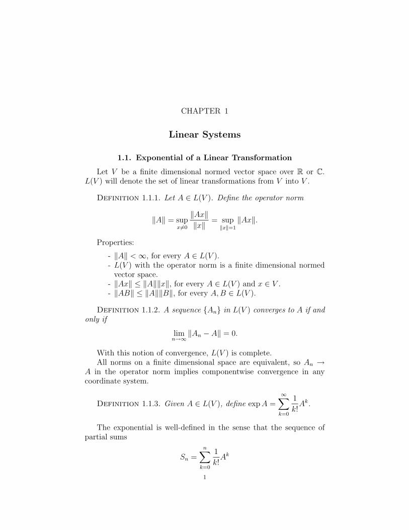
1.1. Exponential of a Linear Transformation
Let V be a finite dimensional normed vector space over R or C.L(V ) will denote the set of linear transformations from V into V .
Definition 1.1.1. Let A ∈ L(V ). Define the operator norm
‖A‖ = supx 6=0
‖Ax‖‖x‖
= sup‖x‖=1
‖Ax‖.
Properties:
- ‖A‖ <∞, for every A ∈ L(V ).- L(V ) with the operator norm is a finite dimensional normed
vector space.- ‖Ax‖ ≤ ‖A‖‖x‖, for every A ∈ L(V ) and x ∈ V .- ‖AB‖ ≤ ‖A‖‖B‖, for every A,B ∈ L(V ).
Definition 1.1.2. A sequence An in L(V ) converges to A if andonly if
limn→∞
‖An − A‖ = 0.
With this notion of convergence, L(V ) is complete.All norms on a finite dimensional space are equivalent, so An →
A in the operator norm implies componentwise convergence in anycoordinate system.
Definition 1.1.3. Given A ∈ L(V ), define expA =∞∑
k=0
1
k!Ak.
The exponential is well-defined in the sense that the sequence ofpartial sums
Sn =n∑
k=0
1
k!Ak
1
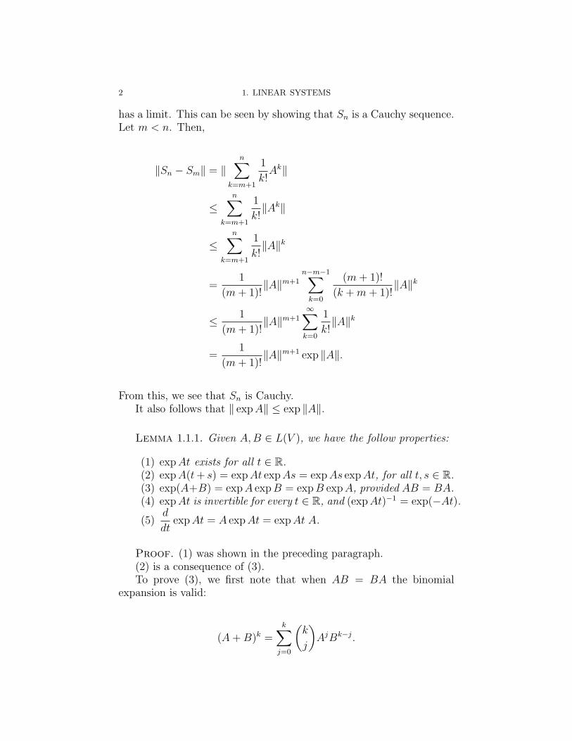
2 1. LINEAR SYSTEMS
has a limit. This can be seen by showing that Sn is a Cauchy sequence.Let m < n. Then,
‖Sn − Sm‖ = ‖n∑
k=m+1
1
k!Ak‖
≤n∑
k=m+1
1
k!‖Ak‖
≤n∑
k=m+1
1
k!‖A‖k
=1
(m+ 1)!‖A‖m+1
n−m−1∑k=0
(m+ 1)!
(k +m+ 1)!‖A‖k
≤ 1
(m+ 1)!‖A‖m+1
∞∑k=0
1
k!‖A‖k
=1
(m+ 1)!‖A‖m+1 exp ‖A‖.
From this, we see that Sn is Cauchy.It also follows that ‖ expA‖ ≤ exp ‖A‖.
Lemma 1.1.1. Given A,B ∈ L(V ), we have the follow properties:
(1) expAt exists for all t ∈ R.(2) expA(t+ s) = expAt expAs = expAs expAt, for all t, s ∈ R.(3) exp(A+B) = expA expB = expB expA, provided AB = BA.(4) expAt is invertible for every t ∈ R, and (expAt)−1 = exp(−At).(5)
d
dtexpAt = A expAt = expAt A.
Proof. (1) was shown in the preceding paragraph.(2) is a consequence of (3).To prove (3), we first note that when AB = BA the binomial
expansion is valid:
(A+B)k =k∑
j=0
(k
j
)AjBk−j.
1.2. SOLUTION OF THE INITIAL VALUE PROBLEM FOR LINEAR HOMOGENEOUS SYSTEMS3
Thus, by definition
exp(A+B) =∞∑
k=0
1
k!(A+B)k
=∞∑
k=0
1
k!
k∑j=0
(k
j
)AjBk−j
=∞∑
j=0
1
j!Aj
∞∑k=j
1
(k − j)!Bk−j
=∞∑
j=0
1
j!Aj
∞∑`=0
1
`!B`
= expA expB.
The rearrangements are justified by the absolute convergence of allseries.
(4) is an immediate consequence of (2).(5) is proven as follows. We have
‖(∆t)−1[expA(t+ ∆t) expAt]− expAt A‖= ‖ expAt(∆t)−1[expA∆t− I]− A‖
=
∥∥∥∥∥expAt∞∑
k=2
(∆t)k−1
k!Ak
∥∥∥∥∥≤ ‖ expAt‖
∥∥∥∥∥A2∆t∞∑
k=2
(∆t)k−2
k!Ak−2
∥∥∥∥∥≤ |∆t|‖A‖2 exp ‖A‖(|t|+ |∆t|).
This last expression tends to 0 as ∆t→ 0. Thus, we have shown thatd
dtexpAt = expAt A. This also equals A expAt because A commutes
with the partial sums for expAt and hence with expAt itself.
1.2. Solution of the Initial Value Problem for LinearHomogeneous Systems
Theorem 1.2.1. Let A be an n×n matrix over R, and let x0 ∈ Rn.The initial value problem
(1.2.1) x′(t) = Ax(t), x(t0) = x0
has a unique solution defined for all t ∈ R given by
(1.2.2) x(t) = expA(t− t0) x0.
4 1. LINEAR SYSTEMS
Proof. We use the method of the integrating factor. Multiplyingthe system (1.2.1) by exp(−At) and using Lemma 1.1.1, we see thatx(t) is a solution of the IVP if and only if
d
dt[exp(−At)x(t)] = 0, x(t0) = x0.
Integration of this identity yields the equivalent statement
exp(−At)x(t)− exp(−At0)x0 = 0,
which in turn is equivalent to (1.2.2). This establishes existence, anduniqueness.
1.3. Computation of the Exponential
The main computational tool will be reduction to an elementarycase by similarity transformation.
Lemma 1.3.1. Let A, S ∈ L(V ) with S invertible. Then
exp(SAS−1) = S(expA)S−1.
Proof. This follows immediately from the definition of the expo-nential together with the fact that (SAS−1)k = SAkS−1, for everyk ∈ N.
The simplest case is that of a diagonal matrixD = diag [λ1, . . . , λn].Since Dk = diag [λk
1, . . . , λkn], we immediately obtain
expDt = diag [expλ1t, . . . , expλnt].
Now if A is diagonalizable, i.e. A = SDS−1, then we can use Lemma1.3.1 to compute
expAt = S expDt S−1.
An n × n matrix A is diagonalizable if and only if there is a ba-sis of eigenvectors vjn
j=1. If such a basis exists, let λjnj=1 be the
corresponding set of eigenvalues. Then
A = SDS−1,
where D = diag [λ1, . . . , λn] and S = [v1 · · · vn] is the matrix whosecolumns are formed by the eigenvectors. Even if A has real entries, itcan have complex eigenvalues, in which case the matrices D and S willhave complex entries. However, if A is real, complex eigenvectors andeigenvalues occur in conjugate pairs.
1.3. COMPUTATION OF THE EXPONENTIAL 5
In the diagonalizable case, the solution of the initial value problem(1.2.1) is
x(t) = expAt x0 = S expDt S−1x0 =n∑
j=1
cj expλjt vj,
where the coefficients cj are the coordinates of the vector c = S−1x0.Thus, the solution space is spanned by the elementary solutions expλjt vj.
There are two important situations where an n × n matrix can bediagonalized.
- A is real and symmetric, i.e. A = AT . Then A has real eigen-values and there exists an orthonormal basis of real eigen-vectors. Using this basis yields an orthogonal diagonalizingmatrix S, i.e. ST = S−1.
- A has distinct eigenvalues. For each eigenvalue there is alwaysat least one eigenvector, and eigenvectors corresponding todistinct eigenvalues are independent. Thus, there is a basis ofeigenvectors.
An n × n matrix over C may not be diagonalizable, but it canalways be reduced to Jordan canonical (or normal) form. A matrix Jis in Jordan canonical form if it is block diagonal
J =
B1
. . .Bp
and each Jordan block has the form
B =
λ 1 0 · · · 00 λ 1 · · · 0
. . .0 0 · · · λ 10 0 · · · 0 λ
.Since B is upper triangular, it has the single eigenvalue λ with multi-plicity equal to the size of the block b.
Computing the exponential of a Jordan block is easy. Write
B = λI +N,
where N has 1’s along the superdiagonal and 0’s everywhere else. Thematrix N is nilpotent. If the block size is d× d, then Nd = 0. We also
6 1. LINEAR SYSTEMS
clearly have that λI and N commute. Therefore,
expBt = exp(λI +N)t = expλIt expNt = exp(λt)d−1∑j=1
tj
j!N j.
The entries of expNt are polynomials in t of degree at most d− 1.Again using the definition of the exponential, we have that the
exponential of a matrix in Jordan canonical form is the block diagonalmatrix
exp Jt =
expB1t. . .
expBpt
.The following central theorem in linear algebra will enable us to
understand the form of expAt for a general matrix A.
Theorem 1.3.1. Let A be an n× n matrix over C. There exists abasis vjn
j=1 for Cn which reduces A to Jordan normal form J . Thatis, if S = [v1 · · · vn] is the matrix whose columns are formed from thebasis vectors, then
A = SJS−1.
The Jordan normal form of A is unique up to the permutation of itsblocks.
When A is diagonalizable, the basis vjnj=1 consists of eigenvectors
of A. In this case, the Jordan blocks are 1 × 1. Thus, each vector vj
lies in the kernel of A− λjI for the corresponding eigenvalue λj.In the general case, the basis vjn
j=1 consists of appropriately cho-sen generalized eigenvectors of A. A vector v is a generalized eigen-vector of A corresponding to an eigenvalue λj if it lies in the kernelof (A − λjI)
k for some k ∈ N. The set of generalized eigenvectorsof A corresponding to a given eigenvalue λj is a subspace, E(λj), ofCn, called the generalized eigenspace of λj. If λjd
j=1 are the distincteigenvalues of A, then
Cn = E(λ1)⊕ · · · ⊕ E(λd),
as a direct sum.We arrive at the following algorithm for computing expAt. Given
an n × n matrix A, reduce it to Jordan canonical form A = SJS−1,and then write
expAt = S exp Jt S−1.
Even if A (and hence also expAt) has real entries, the matrices J andS may have complex entries. However, if A is real, then any complexeigenvalues and generalized eigenvectors occur in conjugate pairs.
1.4. ASYMPTOTIC BEHAVIOR OF LINEAR SYSTEMS 7
1.4. Asymptotic Behavior of Linear Systems
Definition 1.4.1. Let A be an n × n matrix over R. Define thecomplex stable, unstable, and center subspaces of A, denoted EC
s , ECu ,
and ECc , respectively, to be the linear span over C of the generalized
eigenvectors of A corresponding to eigenvalues with negative, positive,and zero real parts, respectively.
Arrange the eigenvalues of A so that Re λ1 ≤ . . . ≤ Re λn. Partitionthe set 1, . . . , n = Js ∪ Jc ∪ Ju so that
Re λj < 0, j ∈ Js
Re λj = 0, j ∈ Jc
Re λj > 0, j ∈ Ju.
Let x1, . . . , xn ∈ Cn be a basis of generalized eigenvectors corre-sponding to the eigenvalues λ1, . . . , λn. Then
span xj : j ∈ Js = ECs
span xj : j ∈ Jc = ECc
span xj : j ∈ Ju = ECu .
It follows that Cn = ECs + EC
c + ECu is a direct sum. Thus, any vector
x ∈ Cn is uniquely represented as
x = Psx+ Pcx+ Pux ∈ ECs + EC
c + ECu .
The maps Ps, Pc, Pu are linear projections onto the complex stable,center, and unstable subspaces. Thus, we have
P 2s = Ps, P 2
c = Pc, P 2u = Pu.
Since these subspaces are independent of each other, we have that
PsPc = PcPs = 0, . . .
Since these subspaces are invariant under A, the projections commutewith A, and thus also any function of A, including expAt.
Since A is real, if v ∈ Cn is a generalized eigenvector with eigenvalueλ ∈ C, then its complex conjugate v is a generalized eigenvector witheigenvalue λ. It follows that the subspaces EC
s , ECc , and EC
u are closedunder complex conjugation. For any vector x ∈ Cn, we have
Psx+ Pcx+ Pux = x = Psx+ Pcx+ Pux.
This gives two representations of x in ECs + EC
c + ECu . By uniqueness
of representations, we must have
Psx = Psx, Pcx = Pcx, Pux = Pux.
8 1. LINEAR SYSTEMS
So if x ∈ Rn, we have that
Psx = Psx, Pcx = Pcx, Pux = Pux.
Therefore, the projections leave Rn invariant:
Ps : Rn → Rn, Pc : Rn → Rn, Pu : Rn → Rn.
Definition 1.4.2. Let A be an n × n matrix over R. Define thereal stable, unstable, and center subspaces of A, denoted Es, Eu, andEc, to be the images of Rn under the corrsponding projections:
Es = Ps Rn, Ec = Pc Rn, Eu = Pu Rn.
We have that Rn = Es +Ec +Eu is a direct sum. When restrictedto Rn, the projections possess the same properties as on Cn.
The real stable subspace can also be characterized as the linear spanover R of the real and imaginary parts of all generalized eigenvectorsof A corresponding to an eigenvalue with negative real part. Similarstatements hold for Ec and Eu.
We are now ready for the main result of this section, which estimatesthe norm of expAt on the invariant subspaces. These estimates will beused many times.
Theorem 1.4.1. Let A an n× n matrix over R. Define
−λs = maxλj : j ∈ Js and λu = minλj : j ∈ Ju.
There is a constant C > 0 and an integer 0 ≤ p < n, depending on A,such that for all x ∈ Cn,
‖ expAt Psx‖ ≤ C(1 + t)pe−λst‖Psx‖, t > 0
‖ expAt Pcx‖ ≤ C(1 + |t|)p‖Pcx‖, t ∈ R‖ expAt Pux‖ ≤ C(1− t)peλut‖Pux‖, t < 0.
Remark: The exponent p in these inequalities has the property thatp+1 is the size of the largest Jordan block corresponding to eigenvaluesλj with j ∈ Js, Jc, Ju, respectively.
Proof. We will prove the first of these inequalities. The other twoare similar.
Let xjnj=1 be a basis generalized eigenvectors with indices ordered
as above. For any x ∈ Cn, we have
x =n∑
j=1
cjxj, and Psx =∑j∈Js
cjxj.
1.4. ASYMPTOTIC BEHAVIOR OF LINEAR SYSTEMS 9
Let S be the matrix whose columns are the vectors xj. Then Sreduces A to Jordan canonical form: A = S(D + N)S−1, where D =diag(λ1, . . . , λn) and Np+1 = 0, form some p < n.
If ejnj=1 is the standard basis, the Sej = xj, and so, ej = S−1xj.
We may write
expAt Psx = S expNt expDt S−1Psx
= S expNt expDt∑j∈Js
cjej
= S expNt∑j∈Js
cj exp(λjt)ej
= S expNt y.
Taking the norm, we have
‖ expAt Psx‖ ≤ ‖S‖‖ expNt y‖.Now, y ∈ span ej : j ∈ Js, and so if p + 1 is the size of the
largest Jordan block corresponding to eigenvalues λj : j ∈ Js, thenNp+1y = 0. Thus, we have that
expNt y =
p∑j=0
tk
k!Nky,
and so, for t > 0,
‖ expNt y‖ ≤p∑
j=0
tk
k!‖N‖k ≤ C1(1 + tp)‖y‖.
Next, we have, for t > 0,
‖y‖2 =
∥∥∥∥∥∑j∈Js
cj exp(λjt)ej
∥∥∥∥∥2
=∑j∈Js
|cj|2 exp(2Re λjt)
≤ exp(−2λst)∑j∈Js
|cj|2
= exp(−2λst)‖S−1Psx‖2
≤ exp(−2λst)‖S−1‖2‖Psx‖2,
and so ‖y‖ ≤ C2 exp(−λst)‖Psx‖.The result follows with C = C1C2.
10 1. LINEAR SYSTEMS
All of the results in this section hold for complex matrices A, ex-cept for the remarks concerning the projections on Rn and the ensuingdefinitions of real invariant subspaces. We will not need this, however.
Notice that for any ε > 0, the function (1+ tp) exp(−εt) is boundedon the interval t > 0. Thus, for any constant 0 < α < λs, we have that
(1 + tp) exp(−λst) = (1 + tp) exp[−(λs − α)t] exp(−αt) ≤ C exp(−αt).It will be convenient to use this slightly weaker version.
CHAPTER 2
Existence Theory
2.1. The Initial Value Problem
Let Ω ⊂ Rn+1 be an open connected set. We will denote points inΩ by (t, x) where t ∈ R and x ∈ Rn. Let f : Ω → Rn be a continuousmap. In this context, f(t, x) is called a vector field on Ω. Given anyinitial point (t0, x0) ∈ Ω, we wish to construct a unique solution to theinitial value problem
(2.1.1) x′(t) = f(t, x(t)) x(t0) = x0.
In order for this to make sense, x(t) must be a C1 function from someinterval I ⊂ R containing the initial time t0 into Rn such that thesolution curve satisfies
(t, x(t)) : t ∈ I ⊂ Ω.
Such a solution is referred to as a local solution when I 6= R. WhenI = R, the solution is called global.
2.2. The Cauchy-Peano Existence Theorem
Theorem 2.2.1 (Cauchy-Peano). If f : Ω → Rn is continuous,then for every point (t0, x0) ∈ Ω the initial value problem (2.1.1) haslocal solution.
The problem with this theorem is that it does not guarantee unique-ness. We will skip the proof, except to mention that it is uses a com-pactness argument based on the Arzela-Ascoli Theorem.
Here is a simple example that demonstrates that uniqueness canindeed fail. Let Ω = R2 and consider the autonomous vector fieldf(t, x) = |x|1/2. When (t0, x0) = (0, 0), the initial value problem hasinfinitely many solutions. In addition to the zero solution x(t) = 0, forany α, β ≥ 0, the following is a family of solutions.
x(t) =
−1
4(t+ α)2, t ≤ −α
0, −α ≤ t ≤ β14(t− β)2, β ≤ t.
This can be verified by direct substitution.
11
12 2. EXISTENCE THEORY
2.3. The Picard Existence Theorem
The failure of uniqueness can be rectified by placing an additionalrestriction on the vector field. The next definition introduces this keyproperty.
Definition 2.3.1. Let Ω ⊂ Rn+1 be an open set. A function f :Ω → Rn is said to be locally Lipschitz continuous in x if for everycompact set K ⊂ Ω, there is a constant CK > 0 such that
‖f(t, x1)− f(t, x2)‖ ≤ CK‖x1 − x2‖,for every (t, x1), (t, x2) ∈ K. If there is a constant for which the in-equality holds for all (t, x1), (t, x2) ∈ Ω, then f is said to be Lipschitzcontinuous in x.
The function ‖x‖α is Lipschitz continuous for α = 1, locally Lip-schitz continuous for α > 1, and not Lipschitz continuous (on anyneighborhood of 0) when α < 1.
Lemma 2.3.1. If f : Ω → Rn is C1, then it is locally Lipschitzcontinuous in x.
Theorem 2.3.1 (Picard). Let Ω ⊂ Rn+1 be open. Assume thatf : Ω → Rn is continuous and that f(t, x) is locally Lischitz continuousin x. Let K ⊂ Ω be any compact set. Then there is a δ > 0 such thatfor every (t0, x0) ∈ K, the initial value problem (2.1.1) has a uniquelocal solution defined on the interval |t− t0| < δ.
Before proving this important theorem, it is convenient to have thefollowing technical “Covering Lemma”.
First, some notaion: Given a point (t, x) ∈ Rn+1 and positive num-bers r and a, define the cylinder
C(t, x) ≡ (t′, x′) ∈ Rn+1 : ‖x− x′‖ ≤ r, |t− t′| ≤ a.
Lemma 2.3.2 (Covering Lemma). Let K ⊂ Ω ⊂ Rn × R with Ωan open set and K a compact set. There exists a compact set K ′ andpositive numbers r and a such that K ⊂ K ′ ⊂ Ω and C(t, x) ⊂ K ′, forall (t, x) ∈ K.
Proof. For every point p = (t, x) ∈ K, choose positive numbersa(p) and r(p) such that
D(p) = (t′, x′) ∈ Rn+1 : ‖x− x′‖ ≤ 2r(p), |t− t′| ≤ 2a(p) ⊂ Ω.
This is possible because Ω is open.Define the cylinders
C(p) = (t′, x′) ∈ Rn+1 : ‖x− x′‖ < r(p), |t− t′| < a(p).
2.3. THE PICARD EXISTENCE THEOREM 13
The collection of open sets C(p) : p ∈ K forms an open cover of theset K. K is compact, therefore there is a finite number of cylindersC(p1), . . . , C(pN) whose union contains K. Set
K ′ = ∪Ni=1D(pi).
Then K ′ is compact, and
K ⊂ ∪Ni=1C(pi) ⊂ ∪N
i=1D(pi) = K ′ ⊂ Ω.
Define
a = mina(pi) : i = 1, . . . , N and r = minr(pi) : i = 1, . . . , N.The claim is that, for this uniform choice of a and r, C(t, x) ⊂ K ′,
for all (t, x) ∈ K.If (t, x) ∈ K, then (t, x) ∈ C(pi) for some i = 1, . . . , N . Let (t′, x′) ∈
C(t, x). Then
‖x′ − xi‖ ≤ ‖x′ − x‖+ ‖x− xi‖ ≤ a+ a(pi) ≤ 2a(pi)
and|t′ − ti| ≤ |t′ − t|+ |t− ti| ≤ r + r(pi) ≤ 2r(pi).
This shows that (t′, x′) ∈ D(pi), from which follows the conclusionC(t, x) ⊂ D(pi) ⊂ K ′.
Proof of the Picard Theorem. The first step of the proof isto reformulate the problem. If x(t) is a C1 solution of the initial valueproblem (2.1.1) for |t− t0| ≤ δ, then by integration we find that
(2.3.1) x(t) = x0 +
∫ t
t0
f(s, x(s))ds,
for |t − t0| ≤ δ. Conversely, if x(t) is a C0 solution of the integralequation, then it is C1 and it solves the initial value problem (2.1.1).
Given a compact subset K ⊂ Ω, choose a, r,K ′ as in the coveringlemma.
Choose (t0, x0) ∈ K. Let δ < a and set
Iδ = ‖t− t0| ≤ δ, Br = ‖x− x0‖ ≤ r, Xδ = C0(Iδ;Br).
Note that Xδ is a complete metric space with the sup norm metric.By definition, if x ∈ Xδ, then
(s, x(s)) ∈ C(t0, x0) ⊂ K ′ ⊂ Ω,
for s ∈ Iδ. Thus, the operator
Tx(t) = x0 +
∫ t
t0
f(s, x(s))ds
is well-defined on Xδ and the function Tx(t) is continuous for t ∈ Iδ.
14 2. EXISTENCE THEORY
Define M1 = maxK′ |f(t, x)|. This claim is that if δ is chosen smallenough so that M1δ ≤ r, then T : Xδ → Xδ. If x ∈ Xδ, we have from(2.3.1)
supIδ
‖Tx(t)− x0‖ ≤M1δ ≤ r,
for t ∈ Iδ.Next, let M2 be a Lipschitz constant for f(t, x) on K ′. If δ is further
restricted so that M2δ < 1/2, then we claim that T : Xδ → Xδ is acontraction. Let x1, x2 ∈ Xδ. Then from (2.3.1), we have
supIδ
‖Tx1(t)− Tx2(t)‖ ≤M2δ supIδ
‖x1(t)− x2(t)‖
≤ 1/2 supIδ
‖x1(t)− x2(t)‖.
So by the Contraction Mapping Principle, there exists a uniquefunction x ∈ Xδ such that Tx = x. In other words, x solves (2.3.1).
Note that the final choice of δ is mina, r/M1, 1/M2 which dependsonly on the set K and on f .
The alert reader will notice that the solution constructed above isunique within the metric space Xδ, but it is not necessarily unique inC0(Iδ, Br). The next result fills in this gap.
Theorem 2.3.2 (Uniqueness). Suppose that f : Ω → Rn satisifesthe hypotheses of the Picard Theorem. For j = 1, 2, let xj(t) be so-lutions of x′(t) = f(t, x(t)) on the interval Ij. If there is a pointt0 ∈ I1 ∩ I2 such that x1(t0) = x2(t0), then x1(t) = x2(t) on the in-terval I1 ∩ I2. Moreover, the function
x(t) =
x1(t), t ∈ I1x2(t), t ∈ I2
defines a solution on the interval I1 ∪ I2.
Proof. Let J ⊂ I1 ∩ I2 be any closed interval with t0 ∈ J . Let Mbe a Lipschitz constant for f(t, x) on the compact set
(t, x1(t)) : t ∈ J ∪ (t, x2(t)) : t ∈ J.The solutions xj(t), j = 1, 2, satisfy the integral equation (2.3.1) onthe interval J . Thus, estimating as before
‖x1(t)− x2(t)‖ ≤∣∣∣∣∫ t
t0
M‖x1(s)− x2(s)‖ds∣∣∣∣ ,
for t ∈ J . It follows from Gronwall’s Lemma (below) that
‖x1(t)− x2(t)‖ = 0
2.4. EXTENSION OF SOLUTIONS 15
for t ∈ J .From this it follows that x(t) is well-defined, is C1, and is a solution.
Lemma 2.3.3 (Gronwall). Let f(t), ϕ(t) be nonnegative continuousfunction on an open interval J = (α, β) containing the point t0. Letc0 ≥ 0. If
f(t) ≤ c0 +
∣∣∣∣∫ t
t0
ϕ(s)f(s)ds
∣∣∣∣ ,for all t ∈ J , then
f(t) ≤ c0 exp
∣∣∣∣∫ t
t0
ϕ(s)ds
∣∣∣∣ ,for t ∈ J .
Proof. Suppose first that t ∈ [t0, β). Define
F (t) = c0 +
∫ t
t0
ϕ(s)f(s)ds.
Then F is C1 and
F ′(t) = ϕ(t)f(t) ≤ ϕ(t)F (t),
for t ∈ [t0, β), since f(t) ≤ F (t). This implies that
d
dt
[exp
(−∫ t
t0
ϕ(s)ds
)F (t)
]≤ 0,
for t ∈ [t0, β). Integrate this over the interval [t0, τ) to get
f(τ) ≤ F (τ) ≤ c0 exp
∫ τ
t0
ϕ(s)ds,
for τ ∈ [t0, β).On the interval (α, t0], perform the analogous argument to the func-
tion
G(t) = c0 +
∫ t0
t
ϕ(s)f(s)ds.
2.4. Extension of Solutions
Theorem 2.4.1. For every (t0, x0) ∈ Ω the solution to the ini-tial value problem (2.1.1) extends to a maximal existence interval I =(α, β). Furthermore, if K ⊂ Ω is any compact set containing the point(t0, x0), then there exist times α(K), β(K) such that (t, x(t)) /∈ K, fort ∈ (α, α(K)) ∪ (β(K), β).
16 2. EXISTENCE THEORY
Proof. Define the sets
A = a < t0 : there exists a solution of the IVP on [a, t0]B = b > t0 : there exists a solution of the IVP on [t0, b].
The existence theorem guarantees that these sets are nonempty, so wemay define
α = inf A and β = supB.
Note that α and/or β could be infinite – that’s ok.Choose sequences αj ∈ A and βj ∈ B with αj ↓ α and βj ↑ β. On
each interval [αj, βj] we have a solution. By the uniqueness theorem(2.3.2), we obtain a unique solution on (α, β).
If (α′, β′) is another interval on which a solution exists, we havethat a ∈ A for all α′ < a < t0. Taking the infimum of all such a wehave that α′ ≥ α. Likewise, we have that β′ ≤ β. Thus, we obtain(α′, β′) ⊂ (α, β), which proves maximality.
Let K ⊂ Ω be compact with (t0, x0) ∈ K. Let |t − t0| < δ be theuniform existence interval given by the existence theorem (2.3.1).
If β = +∞, then choose T > 0 so that K ⊂ [−T, T ] × Rn. Setβ(K) = T . Then β(K) < β and (t, x(t)) /∈ K for t ≥ β(K).
So we may now assume that β < +∞. Define β(K) = β − δ/2.Suppose that (t, x(t)) ∈ K for some t ∈ (β(K), β). Let x(t) solvethe initial value problem with x(t) = x(t). Then we have that x(t) isdefined at least for |t− t| < δ. By the uniqueness theorem (2.3.2), thefunction
x(t) =
x(t), t ∈ (α, β)
x(t), t ∈ (t− δ, t+ δ)
is a well-defined solution passing through the point (t0, x0) on an inter-val which properly contains the maximal interval (α, β), since t + δ >β. From this contradiction, we conclude that (t, x(t)) /∈ K for allt ∈ (β(K), β).
As an example, consider the IVP
x′ = x2, x(0) = x0,
the solution of which is
x(t) =x0
1− x0 t.
2.5. CONTINUOUS DEPENDENCE ON INITIAL CONDITIONS 17
We see that the maximal interval of existence depends on the initialvalue x0:
I = (α, β) =
(−∞,∞), if x0 = 0
(−∞, 1/x0), if x0 > 0
(1/x0,∞), if x0 < 0.
2.5. Continuous Dependence on Initial Conditions
Definition 2.5.1. A function g from Rm into R ∪ ∞ is lowersemi-continuous at a point y0 provided lim inf
y→y0
g(y) ≥ g(y0).
Equivalently, a function g into R ∪ ∞ is lower semi-continuousat a point y0 provided for every L < g(y0) there is a neighborhood V ofy0 such that L ≤ g(y) for y ∈ V .
Let Ω ⊂ Rn+1 be an open set. Let f : (t, x) ∈ Ω → Rn be continuousand locally Lipschitz continuous in x. Given (t0, x0) ∈ Ω, let x(t, t0, x0)denote the unique solution of the IVP
x′ = f(t, x), x(t0) = x0,
with maximal existence interval I(t0, x0) = (α(t0, x0), β(t0, x0)).
Theorem 2.5.1. The domain of x(t, t0, x0), namely
D = (t, t0, x0) : (t0, x0) ∈ Ω, t ∈ I(t0, x0),
is an open set in Rn+2.The function x(t, t0, x0) is continuous on D.The function β(t0, x0) is lower semi-continuous on Ω, and the func-
tion α(t0, x0) is upper semi-continuous on Ω.
Proof. Fix (t0, x0) ∈ Ω. We will use the abbreviations x0(t) =x(t, t0, x0), α0 = α(t0, x0), and β0 = β(t0, x0).
CLAIM. Choose any pair α, β such that β0 < β < α < α0. Givenany ε > 0, there exists a neighborhood V ⊂ Ω containing the point(t0, x0) such that for any (t1, x1) ∈ V , the solution x1(t) = x(t, t1, x1)is defined for t ∈ [α, β], and
‖x1(t)− x0(t)‖ < ε,
for t ∈ [α, β].Let’s assume that the CLAIM holds and use it to establish the
theorem.To show that x(t, t0, x0) is continuous, fix (t′, t0, x0) ∈ D and let
ε > 0 be given. Choose α, β such that α0 < α < t′ < β < β0.
18 2. EXISTENCE THEORY
By the CLAIM, there is a neighborhood (t0, x0) ∈ V ⊂ Ω such thatx1(t) = x(t, t1, x1) is defined for (t1, x1) ∈ V , t ∈ [α, β], and
‖x1(t)− x0(t)‖ < ε/2,
for t ∈ [α, β].Now x0(t) is continuous as a function of t on [α, β], since it’s a
solution of the IVP. So there is a δ > 0 with |t − t′| < δ ⊂ [α, β],such that
‖x0(t)− x0(t′)‖ < ε/2,
provided |t− t′| < δ.For any (t, t1, x1) ∈ |t− t′| < δ × V , we have that
‖x(t, t1, x1)− x(t′, t0, x0)‖ ≤ ‖x(t, t1, x1)− x(t, t0, x0)‖+ ‖x(t, t0, x0)− x(t′, t0, x0)‖
≤ ε/2 + ε/2 = ε.
This proves continuity.Let (t′, t0, x0) ∈ D. In the preceding, we have seen that the set
|t− t′| < δ × V is a neighborhood of (t′, t0, x0) which is contained inD. This shows that D is open.
Using the CLAIM again, we have that for any β < β0, there is aneighborhood V ⊂ Ω of (t0, x0) such that (t1, x1) ∈ V implies thatx(t, t1, x1) is defined for t ∈ [t1, β]. This says that β(t1, x1) ≥ β, whichin turn means that β is lower semi-continuous at (t0, x0). The proofthat α is upper semi-continuous is similar.
It remains to prove the CLAIM.Consider the compact set K = (s, x0(s)) : s ∈ [α, β]. By the
covering lemma, there exist a compact set K ′ and numbers a, r > 0such that K ⊂ K ′ ⊂ Ω and
C(s, x0(s)) = (s′, x′) : |s′ − s| < a, ‖x′ − x0(s)‖ < r ⊂ K ′,
for all s ∈ [α, β]. Define M1 = maxK′
‖f(t, x)‖ and let M2 be a Lipschitz
constant for f on K ′.Given 0 < ε < r, choose δ small enough so that δ < a, δ < r,
|t− t0| < δ ⊂ [α, β], and
δ(M1 + 1) expM2(β − α) < ε < r.
Set V = (t, x) : |t − t0| < δ, ‖x − x0‖ < δ. Notice that V ⊂C(t0, x0) ⊂ K ′.
2.5. CONTINUOUS DEPENDENCE ON INITIAL CONDITIONS 19
For |t1 − t0| < δ, we have
‖x0(t1)− x0‖ = ‖∫ t1
t0
f(s, x0(s))ds‖
≤M1|t1 − t0|≤M1δ.
Now let x1(t) = x(t, t1, x1) which is defined on the maximal interval(α(t1, x1), β(t1, x1)) = (α1, β1). Define
t∗ = supt : (s, x1(s)) ∈ K ′, s ∈ [t1, t].
Since (t, x1(t)) must eventually exit K ′, we have that t∗ < β1. Fort < min(t∗, β), we have that (t, xi(t)) ∈ K ′, i = 1, 2.
Since
xi(t) = xi +
∫ t
ti
f(s, xi(s))ds,
i = 1, 2, we have
x1(t)− x0(t) = x1 − x0 +
∫ t
t1
f(s, x1(s))ds−∫ t
t0
f(s, x0(s))ds
= x1 − x0 + x0 − x0(t1) +
∫ t
t1
[f(s, x1(s))− f(s, x0(s))]ds,
For t1 < t < min(t∗, β), we now have the following estimate:
‖x1(t)− x0(t)‖ ≤ ‖x1 − x0‖+ ‖x0 − x0(t1)‖
+
∫ t
t1
‖f(s, x1(s))− f(s, x0(s))‖ds
≤ δ(1 +M1) +
∫ t
t1
M2‖x1(s)− x0(s)‖ds.
By Gronwall’s inequality and our choice of δ, we obtain
‖x1(t)− x0(t)‖ ≤ δ(1 +M1) expM2[t− t1] ≤ ε < r,
for t1 < t < min(t∗, β). Throughout this time interval, we see that(t, x1(t)) ∈ C(t, x0(t)) ⊂ K ′. Thus, we have shown that β1 > t∗ ≥ β,and that x1(t) remains within ε of x0(t). This completes the proof ofthe CLAIM.
20 2. EXISTENCE THEORY
2.6. Flow of a Nonautonomous System
Let f : Ω → Rn be a vector field which satisfies the hypothesesof the Picard Theorem 2.3.1. Given (t0, x0) ∈ Ω, let x(t, t0, x0) bethe corresponding solution of the initial value problem defined on themaximal existence interval I(t0, x0) = (α(t0, x0), β(t0, x0)). Recall thatthe domain of x(t, t0, x0) is
D = (t, t0, x0) ∈ Rn+2 : (t0, x0) ∈ Ω, t ∈ I(t0, x0).
Lemma 2.6.1. Let (s, t0, x0) ∈ D. Then
I(t0, x0) = I(s, x(s, t0, x0))
andx(t, t0, x0) = x(t, s, x(s, t0, x0))
for all t ∈ I(t0, x0).
Proof. This is a consequence of the uniqueness theorem (2.3.2).Both solutions pass through the point (s, x(s, t0, x0)), and so they sharethe same maximal existence interval and they agree on that interval.
Lemma 2.6.2. If (s, t0, x0) ∈ D, then (t0, s, x(s, t0, x0)) ∈ D and
x(t0, s, x(s, t0, x0)) = x0.
Proof. Let (s, t0, x0) ∈ D. Then by Lemma (2.6.1), we have
t0 ∈ I(t0, x0) = I(s, x(s, t0, x0),
and we may substitute t0 for t to get the result:
x0 = x(t0, t0, x0) = x(t0, s, x(s, t0, x0)).
Definition 2.6.1. Let t, s ∈ R. The flow of the vector field f fromtime s to time t is the map Φt,s(y) ≡ x(t, s, y). The domain of the flowmap is therefore the set
U(t, s) ≡ y ∈ Rn : t ∈ I(s, y).
Notice that U(t, s) ⊂ Rn is open because the domain D is open. Itis possible that U(t, s) is empty for some pairs t, s.
Lemma 2.6.1 says that
Φs,t0 : U(t, t0) ∩ U(s, t0) → U(t, s)
and
Φt,t0(y) = Φt,s Φs,t0(y), y ∈ U(t, t0) ∩ U(s, t0).
2.7. FLOW OF AUTONOMOUS SYSTEMS 21
Lemma 2.6.2 says that
Φs,t0 : U(s, t0) → U(t0, s)
and
Φt0,s Φs,t0(y) = y, y ∈ U(s, t0).
It follows that Φs,t0 is a homeomorphism from U(s, t0) onto U(t0, s).
2.7. Flow of Autonomous Systems
Suppose now that the vector field f(t, x) = f(x) is autonomous.Then we may assume that its domain has the form Ω = R×O for anopen set O ⊂ Rn.
Lemma 2.7.1. Let x0 ∈ O, t, τ ∈ R. Then
t+ τ ∈ I(t0, x0) if and only if t ∈ I(t0 − τ, x0),
and
x(t+ τ, t0, x0) = x(t, t0 − τ, x0), for t ∈ I(t0 − τ, x0).
Proof. Let y(t) = x(t+ τ, t0, x0). The function y(t) is defined forall t ∈ J = t : t+ τ ∈ I(t0, x0). Since the system is autonomous, y(t)solves the equation y′ = f(y) on the interval J . Since y(t0 − τ) = x0,it follow by the uniqueness theorem 2.3.2 that
x(t+ τ, t0, x0) = x(t, t0 − τ, x0),
and I(t0, x0) = J .
Lemma 2.7.1 says that
U(t+ τ, t0) = U(t, t0 − τ)
and
Φt+τ,t0 = Φt,t0−τ .
If we combine this fact with the general result, we have that
Φt+s,0 = Φt+s,s Φs,0 = Φt,0 Φs,0,
on the domain U(t+ s, 0) ∩ U(s, 0).
Definition 2.7.1. Given x0 ∈ O, define the orbit of x0 to be thecurve
γ(x0) = x(t, 0, x0) : t ∈ I(0, x0).
22 2. EXISTENCE THEORY
Notice that the orbit is a curve in the phase space O ⊂ Rn, asopposed to the solution trajectory (t, x(t, t0, x0)) : t ∈ I(t0, x0) whichis a curve in the space-time domain Ω ⊂ Rn+1.
For autonomous flow, we have the following strengthening of theUniqueness Theorem 2.3.2.
Theorem 2.7.1. If z ∈ γ(x0), then γ(x0) = γ(z). Thus, if twoorbits intersect, then they are identical.
Proof. Suppose that z ∈ γ(x0). This means that z = x(t0, 0, x0)for t0 ∈ I(0, x0). Or in terms of the flow, this says that z = Φt0,0(x0).
Using the property of autonomous flow, we have
Φt,0(x0) = Φt−t0,0 Φt0,0(x0) = Φt−t0,0(z).
This shows that an arbitrary point Φt,0(x0) ∈ γ(x0) belongs to γ(z).Replacing t with t+ t0 shows that an arbitrary point Φt,0(z) ∈ γ(z)
belongs to γ(x0).Thus, γ(x0) = γ(z).
From the existence and uniqueness theory for general systems, wehave that the domain Ω is foliated by the solution trajectories
(t, x(t, t0, x0)) : t ∈ I(t0, x0).
That is, every point (t0, x0) ∈ Ω has a unique trajectory passingthrough it. This result says that, for autonomous systems, the phasespace O is foliated by the orbits.
Since x′ = f(x), the orbits are curves in O everywhere tangent tothe vector field f(x). They are sometimes also referred to as integralcurves. They can be obtained by solving the system
dx1
f1(x)= . . . =
dxn
fn(x).
For example, consider the harmonic oscillator
x′1 = x2, x′2 = −x1.
The system for the integral curves is
dx1
x2
=dx2
−x1
.
Solutions satisfy
x21 + x2
2 = c,
and so we confirm that the orbits are concentric circles centered at theorigin.
2.8. GLOBAL SOLUTIONS 23
2.8. Global Solutions
As usual, we assume that f : Ω → Rn satisfies the hypotheses ofthe Picard Existence Theorem 2.3.1.
Recall that a global solution of the initial value problem is onewhose maximal interval of existence is R. For this to be possible, it isnecessary for the domain Ω to be unbounded in the time direction. Solet’s assume that Ω = R×O, where O ⊂ Rn is open.
Theorem 2.8.1. Let I = (α, β) be the maximal interval of existenceof some solution x(t) of the initial value problem. Then either β = +∞or for every compact set K ⊂ O, there exists a time β(K) < β suchthat x(t) /∈ K for all t ∈ (β(K), β).
Proof. Assume that β < +∞. Suppose that K ⊂ O is compact.Then K ′ = [t0, β]×K ⊂ Ω is compact. By Theorem 2.4.1, there existsa time β(K ′) < β such that (t, x(t)) /∈ K ′ for t ∈ (β(K ′), β). Sincet < β, this implies that x(t) /∈ K for t ∈ (β(K ′), β).
Of course, the analogous result holds for α, the left endpoint of I.
Theorem 2.8.2. If Ω = Rn+1, then either β = +∞ or
limt→β−
‖x(t)‖ = +∞.
Proof. If β < +∞, then by the previous result, for every R > 0,there is a time β(R) such that x(t) /∈ x : ‖x‖ ≤ R for t ∈ (β(R), β).In other words, ‖x(t)‖ > R for t ∈ (β(R), β), i.e. the desired conclusionholds.
Corollary 2.8.1. Assume that Ω = Rn+1. If there exists a non-negative continuous function ψ(t) defined for all t ∈ R such that
‖x(t)‖ ≤ ψ(t) for all t ∈ [t0, β),
then β = +∞.
Proof. The assumed estimate implies that ‖x(t)‖ remains boundedon any bounded time interval. By the previous result, we must havethat β = +∞.
Theorem 2.8.3. Let Ω = Rn+1. Suppose that there exist continuousnonnegative functions c1(t), c2(t) defined on R such that the vector fieldf satisfies
‖f(t, x)‖ ≤ c1(t)‖x‖+ c2(t), for all (t, x) ∈ Rn+1.
Then the solution to the initial value problem is global, for every (t0, x0) ∈Rn+1.
24 2. EXISTENCE THEORY
Proof. We know that a solution of the initial value problem alsosolves the integral equation
x(t) = x0 +
∫ t
t0
f(s, x(s))ds,
for all t ∈ (α, β). Applying the estimate for ‖f(t, x)‖, we find that
‖x(t)‖ ≤ ‖x0‖+
∣∣∣∣∫ t
t0
[c1(s)‖x(s)‖+ c2(s)]ds
∣∣∣∣≤ ‖x0‖+
∣∣∣∣∫ t
t0
c2(s)ds
∣∣∣∣+ ∣∣∣∣∫ t
t0
c1(s)‖x(s)‖ds∣∣∣∣ .
Our version of Gronwall’s inequality 2.3.3 can easily be adapted to thisslightly more general situation. Fix T ∈ R, and define
CT = max
‖x0‖+
∣∣∣∣∫ t
t0
c2(s)ds
∣∣∣∣ : |t− t0| ≤ |T |.
Then for t ∈ |t− t0| ≤ |T |, we have by Gronwall’s inequality 2.3.3
‖x(t)‖ ≤ CT exp
∣∣∣∣∫ t
t0
c1(s)‖x(s)‖ds∣∣∣∣ .
In particular, this holds for t = T . Thus, by Corollary 2.8.1, we havethat β = +∞ (and α = −∞).
Corollary 2.8.2. Let A(t) be an n× n matrix and let F (t) be ann-vector which depend continuously on t ∈ R. Then the linear initialvalue problem
x′(t) = A(t)x(t) + F (t), x(t0) = x0
have a unique global solution for every (t0, x0) ∈ Rn+1.
Proof. This is an immediate corollary of the preceding result,since the vector field
f(t, x) = A(t)x+ F (t)
satisfies
‖f(t, x)‖ ≤ ‖A(t)‖‖x‖+ ‖F (t)‖.
2.9. STABILITY 25
2.9. Stability
Let Ω = R × O for some open set O ⊂ Rn, and suppose thatf : Ω → Rn satisfies the hypotheses of the Picard Theorem.
Definition 2.9.1. A point x ∈ O is called an equilibrium point(singular point, critical point) if f(t, x) = 0, for all t ∈ R.
Definition 2.9.2.An equilibrium point x is stable if given any ε > 0 and t0 > 0 there
exists a δ = δ(ε, t0) such that for all ‖x0 − x‖ < ε, the solution of theinitial value problem x(t, t0, x0) exists for all t ≥ t0 and
‖x(t, t0, x0)− x‖ < ε, t ≥ t0.
An equilibrium point x is asymptotically stable if it is stable andthere exists a b(t0) > 0 such that if ‖x0 − x‖ < b(t0), then
limt→∞
‖x(t, t0, x0)− x‖ = 0.
An equilibrium point x is unstable if it is not stable.
Examples:
- A center in R2 is stable, but not asymptotically stable.- A sink or a spiral sink is asymptotically stable.- A saddle is unstable.
Theorem 2.9.1. Let A be an n× n matrix over R, and define thelinear vector field f(x) = Ax.
If Re λ < 0 for all eigenvalues of A, then x = 0 is asymptoticallystable.
If Re λ ≤ 0 for all eigenvalues of A, and A has no generalizedeigenvectors corresponding to eigenvalues with Re λ = 0, then x = 0 isstable.
If Re λ > 0 for at least one eigenvalue of A, then x = 0 is unstable.
Proof. Recall that the solution of the initial value problem isx(t, t0, x0) = expA(t− t0) x0.
If Re λ < 0 for all eigenvalues, then Es = Rn and by Theorem 1.4.1,
‖x(t, t0, x0)‖ ≤ C(1 + (t− t0)p) exp[−λs(t− t0)]‖x0‖,
for all t > t0. Asymptotic stability follows from this estimate.If Re λ ≤ 0 for all eigenvalues, then Es +Ec = Rn and by Theorem
1.4.1,
‖x(t, t0, x0)‖ = ‖ expA(t− t0) (Ps + Pu)x0‖≤ C(1 + (t− t0)
p1) exp[−λs(t− t0)]‖Psx0‖+ C(1 + (t− t0)
p2)‖Pcx0‖,
26 2. EXISTENCE THEORY
for all t > t0.Now if A has no generalized eigenvectors corresponding to eigenval-
ues with Re λ = 0, then all Jordan blocks corresponding to eigenvalueswith zero real part are 1×1. This means that we can take p2 = 0, above.Thus, the right-hand side is bounded by C‖x0‖. Stability follows fromthis estimate.
Suppose that x0 is an eigenvector corresponding to an eigenvaluewith Re λ > 0. For any δ > 0, Re [expλ(t − t0) δx0] is a solutionwhose initial data is arbitrarily small and whose norm is unbounded ast→∞. This proves that the origin is unstable.
Theorem 2.9.2. Let O ⊂ Rn be an open set, and let f : O → Rn beC1. Suppose that x ∈ O is an equilibrium point of f and that the eigen-values of A = Df(x) all satisfy Re λ < 0. Then x is asymptoticallystable.
Proof. Let g(y) = f(x+ y)−Ay. Then g ∈ C1(O), g(0) = 0, andDg(0) = 0.
Asymptotic stability of the equilibrium x = x for the system x′ =f(x) is equivalent to asymptotic stability of the equilibrium y = 0 forthe system y′ = Ay + g(y).
Since Re λ < 0 for all eigenvalues of A, know that from Theoremlin-asym-est that there exists λs > 0 such that
‖ expA(t− t0)‖ ≤ C0(1 + (t− t0)p] exp[−λs(t− t0)], t ≥ t0.
Thus, for any 0 < α < λs, we have
‖ expA(t− t0)‖ ≤ C1 exp[−α(t− t0)], t ≥ t0,
for an appropriate constant C1 > C0.Since Dg(y) is continuous and Dg(0) = 0, given ρ < α, there is a
δ > 0 such that
‖Dg(y)‖ ≤ ρ, for ‖y‖ ≤ δ.
using the elementary Taylor expansion, we see that
g(y) =
∫ 1
0
d
ds[g(sy)]ds =
∫ 1
0
Dg(sy)yds.
Thus, for ‖y‖ ≤ δ, we have
‖g(y)‖ ≤∫ 1
0
‖Dg(sy)‖‖y‖ds ≤ ρ‖y‖.
2.10. LIAPUNOV STABILITY 27
Choose δ < ρ as above, and assume that ‖y0‖ < δ. Let y(t) =y(t, 0, y0) be the solution of the initial value problem
(2.9.1) y′(t) = Ay(t) + g(y(t)), y(0) = y0,
defined for t ∈ (α, β). Define
T = supt : ‖y(s)‖ ≤ ρ for 0 ≤ s ≤ t.Then T > 0, by continuity, and of course, T ≤ β.
If we treat g(y(t)) as an inhomogeneous term, then by the variationof parameters formula
y(t) = expAt y0 +
∫ t
0
expA(t− s)g(y(s))ds.
Thus, on the interval [0, T ], we have
‖y(t)‖ ≤ C1e−αt‖y0‖+
∫ t
0
e−α(t−s)ρ‖y(s)‖ds.
Set z(t) = eαt‖y(t)‖. Then
z(t) ≤ C1‖y0‖+
∫ t
0
ρz(s)ds.
By the Gronwall inequality 2.3.3, we obtain
z(t) ≤ C1‖y0‖eC1ρt, 0 ≤ t ≤ T.
In other words, we have
‖y(t)‖ ≤ C1‖y0‖e(C1ρ−α)t ≤ C1δe(C1ρ−α)t, 0 ≤ t ≤ T.
So now, choose ρ small enough so that C1ρ−α < 0, and choose δ smallenough so that δ < ρ and C1δ < ρ. The preceding estimate shows that‖y(t)‖ < ρ throughout its interval of existence, and thus, by Corollary2.8.1, we have that β = +∞. Thus, we have shown that the origin isstable for the initial value problem (2.9.1). The estimate also showsthat ‖y(t)‖ → 0, as t → ∞, which establishes asymptotic stability ofthe origin.
2.10. Liapunov Stability
Let f(x) be a locally Lipschitz continuous vector field on an openset O ⊂ Rn. Assume that f has an equilibrium point at x ∈ O.
Definition 2.10.1. Let U ⊂ O be a neighborhood of x. A Liapunovfunction for an equilibrium point x of a vector field f is a functionE : U → R such that
(i) E ∈ C(U) ∩ C1(U \ x),
28 2. EXISTENCE THEORY
(ii) E(x) > 0 for x ∈ U \ x and E(x) = 0,(iii) DE(x) f(x) ≤ 0 for x ∈ U \ x.If strict inequality holds in (iii), then E is called a strict Liapunov
function.
Theorem 2.10.1. If an equilibrium point x of f has a Liapunovfunction, then it is stable.
If x has a strict Liapunov function, then it is asymptotically stable.
Proof. Suppose that E is a Liapunov function for x.Choose any ε > 0 such that Bε(x) ⊂ U . Define
m = minE(x) : ‖x‖ = ε and Uε = x ∈ U : E(x) < m ∩Bε(x).
Notice that Uε ⊂ U is a neighborhood of x.The claim is that for any x0 ∈ Uε, the solution x(t) = x(t, 0, x0) of
the IVP x′ = f(x), x(0) = x0 is defined for all t ≥ 0 and remains in Uε.By the local existence theorem and continuity of x(t), we have that
x(t) ∈ Uε on some nonempty interval of the form [0, τ). Let [0, T ) bethe maximal such interval. The claim amounts to showing that T = ∞.
On the interval [0, T ), we have that x(t) ∈ Uε ⊂ U and since E is aLiapunov function,
d
dtE(x(t)) = DE(x(t)) · x′(t) = DE(x(t)) · f(x(t)) ≤ 0.
From this it follows that
(2.10.1) E(x(t)) ≤ E(x(0)) = E(x0) < m,
on [0, T ).Suppose that T < ∞. Then since ‖x(t)‖ < ε for t < T , we have
that the solution x(t) is defined on the interval [0, T ] and ‖x(T )‖ ≤ ε.From the inequality (2.10.1), we have that E(x(T )) < m. Thus, itcannot be that ‖x(T )‖ = ε. Thus, x(T ) ∈ Uε, but this contradicts themaximallity of the interval [0, T ). It follows that T = ∞.
We now use the claim to establish stabilty. Let ε > 0 be given.Without loss of generality, we may assume that Bε(x) ⊂ U . Chooseδ > 0 so that Bδ(x) ⊂ Uε. Then for every x0 ∈ Bδ(x), we have thatx(t) ∈ Uε ⊂ Bε(x), for all t > 0.
To prove the second statement of the theorem, suppose now thatE is a strict Liapunov function.
The equilibrium x is stable, so given ε > 0 with Bε(x) ⊂ U , thereis a δ > 0 so that x0 ∈ Bδ(x) implies x(t) ∈ Bε(x), for all t > 0.
Let x0 ∈ Bδ(x). We must show that x(t) = x(t, 0, x0) satisfieslimt→∞
x(t) = x. We may assume that x0 6= x.
2.10. LIAPUNOV STABILITY 29
Since E is strict and x(t) 6= x, we have that
d
dtE(x(t)) = DE(x(t)) · x′(t) = DE(x(t)) · f(x(t)) < 0.
Thus, E(x(t)) is a monotonically decreasing function bounded belowby 0. Set E∗ = infE(x(t)) : t > 0. Then E(x(t)) ↓ E∗.
Since the solution x(t) remains in the bounded set Uε, it has a limitpoint. That is, there exist a point z ∈ U ε and a sequence of timestk →∞ such that x(tk) → z.
Let s > 0. By the properties of autonomous flow, we have that
x(s+ tk) = x(s+ tk, 0, x0)
= Φs+tk,0(x0)
= Φs,0 Φtk,0(x0)
= x(s, 0, x(tk, 0, x0))
= x(s, 0, x(tk)).
By continuous dependence on initial conditions, we have that
limk→∞
x(s+ tk) = limk→∞
x(s, 0, x(tk)) = x(s, 0, z).
From this it follows that
E∗ = limk→∞
E(x(s+ tk)) = E(x(s, 0, z)).
Thus, x(s, 0, z) is a solution along which E is constant. On the otherhand, we know that if z 6= x0, then E(x(s, 0, z)) is monotonically de-creasing. The conclusion therefore is that z = x.
We have shown that the unique limit point of x(t) is x which equiv-alent to lim
t→∞x(t) = x.
Examples.
- Hamiltonian SystemsLet H : R2 → R be a C1 function. A system of the form
p = Hq(p, q)
q = −Hp(p, q)
is referred to as Hamiltonian, the function H being called theHamiltonian. Suppose that H(0, 0) = 0 and H(p, q) > 0, for(p, q) 6= (0, 0). Then since the origin is a minimum for H, wehave that Hp(0, 0) = Hq(0, 0) = 0. In other words, the originis an equilibrium for the system. Moreover, it is easy to verifythat the Hamiltonian H satisfies the criteria of a Liapunovfunction. Therefore, the origin is stable.
30 2. EXISTENCE THEORY
More generally, we may take H : R2n → R in C1. Againwith H(0, 0) = 0 and H(p, q) > 0, for (p, q) 6= (0, 0), the originis stable.
- Newton’s equationLet G : R → R be C1, with G(0) = 0 and G(u) > 0, for
u 6= 0. Consider the second order equation
u+G′(u) = 0.
With x1 = u and x2 = u, this is equivalent to the first ordersystem
x1 = x2, x2 = −G′(x1).
Notice that the origin is an equilibrium, since G′(0) = 0. Thesystem is, in fact, Hamiltonian with H(x1, x2) = 1
2x2
2 +G(x1).Since H is positive away from the equilibrium, we have thatthe origin is stable.
The nonlinear pendulum arises when G(u) = 1− cosu.- Van der Pol’s equation
Let Φ : R → R be C1, with Φ(0) = 0 and Φ′(u) ≥ 0. Vander Pol’s equation is
u+ Φ′(u) + u = 0.
We rewrite this as a first order system in a nonstandard way.Let
x1 = u, x2 = u+ Φ(u).
Thenx1 = x2 − Φ(x1), x2 = −x1,
and the origin is an equilibrium.The function E(x) = 1
2[x2
1 + x22] serves as a Liapunov func-
tion at the origin, since
DE(x)f(x) = −x1Φ(x1) ≤ 0,
by our assumptions on Φ. If Φ′(u) > 0, for u 6= 0, then theorigin is actually asymptotically stable, although this does notfollow from Theorem 2.10.1.
CHAPTER 3
Nonautonmous Linear Systems
3.1. Fundamental Matrices
Let t 7→ A(t) be a continuous map from R into the set of n × nmatrices over R. Recall that, according to Corollary 2.8.2, the initialvalue problem
x′(t) = A(t)x(t), x(t0) = x0,
has a unique global solution x(t, t0, x0) for all (t0, x0) ∈ Rn+1.By linearity and the Uniqueness Theorem 2.3.2, it follows that
x(t, t0, c1x1 + c2x2) = c1x(t, t0, x1) + c2x(t, t0, x2).
In other words, the flow map Φt,t0(x0) is linear in x0. Thus, there is acontinuous n× n matrix X(t, t0) such that
Φt,t0(x0) = x(t, t0, x0) = X(t, t0)x0.
The matrix X(t, t0) is called the fundamental matrix for A(t).By the general properties of the flow map, we have that
Φt,s Φs,t0 = Φt,t0 , Φt,t = id, Φ−1t,t0
= Φt0,t.
In the linear context, this implies that
X(t, s)X(s, t0) = X(t, t0), X(t, t) = I, X(t, t0)−1 = X(t0, t).
Of course, if A(t) = A is constant, then X(t, t0) = expA(t−t0), andthe preceding relations reflect the familiar properties of the exponentialmatrix for A.
Since
d
dtX(t, t0)x0 =
d
dtx(t, t0, x0) = A(t)x(t, t0, x0) = A(t)X(t, t0)x0,
for every x0 ∈ Rn, we see that X(t, t0) is a matrix solution of
d
dtX(t, t0) = A(t)X(t, t0), X(t0, t0) = I.
The ith column of X(t, t0), namely yi(t) = X(t, t0)ei, satisfies
d
dtyi(t) = A(t)yi(t), yi(t0) = ei.
31
32 3. NONAUTONMOUS LINEAR SYSTEMS
Since this problem has a unique solution for each i = 1, . . . , n, it followsthat X(t, t0) is unique.
From the formula x(t, t0, x0) = X(t, t0)x0, we have that every so-lution is a linear combination of the solutions yi(t). We say that theyi(t) span the solution space.
The next result generalizes our earlier Variation of Parameters for-mula to the case where the coefficient matrix is not constant.
Theorem 3.1.1 (Variation of Parameters). Let t 7→ A(t) be a con-tinuous map from R into the set of n×n matrices over R. Let t 7→ F (t)be a continuous map from R into Rn. Then for every (t0, x0) ∈ Rn, theinitial value problem
x′(t) = A(t)x(t) + F (t), x(t0) = x0,
has a unique global solution x(t, t0, x0), given by the formula
x(t, t0, x0) = X(t, t0)x0 +
∫ t
t0
X(t, s)F (s)ds.
Proof. Global existence and uniqueness was shown in Corollary2.8.2. So we need only verify that the solution x(t) = x(t, t0, x0) satis-fies the given formula.
Let Z(t, t0) be the fundamental matrix for −A(t)T . Set Y (t, t0) =Z(t, t0)
T . Then
d
dtY (t, t0) =
d
dtZ(t, t0)
T = [−A(t)Z(t, t0)]T = −Y (t, t0)A(t),
and so
d
dt[Y (t, t0)X(t, t0)] = [
d
dtY (t, t0)]X(t, t0) + Y (t, t0)[
d
dtX(t, t0)]
= −Y (t, t0)A(t)X(t, t0) + Y (t, t0)A(t)X(t, t0)
= 0.
Therefore, Y (t, t0)X(t, t0) = Y (t, t0)X(t, t0)|t=t0 = I. In other words,we have that Y (t, t0) = X(t, t0)
−1.Now we mimic our previous derivation based on the integrating
factor.
d
dt[Y (t, t0)x(t)] = [
d
dtY (t, t0)]x(t) + Y (t, t0)[
d
dtx(t)]
= −Y (t, t0)A(t)x(t) + Y (t, t0)[A(t)x(t) + F (t)]
= Y (t, t0)F (t).
3.1. FUNDAMENTAL MATRICES 33
Upon integration, we find
x(t) = Y (t, t0)−1x0 +
∫ t
t0
Y (t, t0)−1Y (s, t0)F (s)ds
= X(t, t0)x0 +
∫ t
t0
X(t, t0)X(s, t0)−1F (s)ds
= X(t, t0)x0 +
∫ t
t0
X(t, t0)X(t0, s)F (s)ds
= X(t, t0)x0 +
∫ t
t0
X(t, s)F (s)ds.
Although in general, there is no formula for the fundamental matrix,there is a formula for its determinant.
Theorem 3.1.2. If X(t, t0) is the fundamental matrix for A(t),then
detX(t, t0) = exp
∫ t
t0
tr A(s)ds.
Proof. Regard the determinant of as a multi-linear function ∆ ofthe rows Xi(t, t0) of X(t, t0). Then using multi-linearity, we have
d
dtdetX(t, t0) =
d
dt∆
X1(t, t0)...
Xn(t, t0)
= ∆
X ′1(t, t0)
...Xn(t, t0)
+ . . .+ ∆
X1(t, t0)...
X ′n(t, t0)
.From the differential equation, X ′(t, t0) = A(t)X(t, t0), we get for eachrow
X ′i(t, t0) =
n∑j=1
Aij(t)Xj(t, t0).
34 3. NONAUTONMOUS LINEAR SYSTEMS
Thus, using multi-linearity and the property that ∆ = 0 if two rowsare equal, we obtain
∆
X1(t, t0)
...X ′
i(t, t0)...
Xn(t, t0)
= ∆
X1(t, t0)
...∑nj=1Aij(t)Xj(t, t0)
...Xn(t, t0)
=n∑
j=1
Aij(t)∆
X1(t, t0)
...Xj(t, t0)
...Xn(t, t0)
= Aii(t)∆
X1(t, t0)
...Xi(t, t0)
...Xn(t, t0)
= Aii(t) detX(t, t0).
The result now follows if we substitute this above.
3.2. Floquet Theory
Let A(t) be a real n× n defined and continuous for t ∈ R. Assumethat A(t) is T -periodic for some T > 0. Let X(t) = X(t, 0) be thefundamental matrix for A(t). We shall examine the form of X(t).
Theorem 3.2.1. There n× n matrices P (t), L such that
X(t) = P (t) expLt,
where P (t) is C1 and T -periodic and L is constant.
Remarks:
- Theorem 3.2.1 also holds for complex A(t).- Even if A(t) is real, P (t) and L need not be real.- P (t) and L are not unique.
For example, let S be an invertible matrix which trans-forms L to Jordan normal form J = diag[B1, . . . , Bp]. For
each Jordan block Bj = λjI +N , let Bj = (λj +2πikj
T)I +N ,
for some kj ∈ Z. Then Bj commutes with Bj and
exp(Bj − Bj)T = exp 2πikjI = I.
Define J = diag[B1, . . . , Bp] and L = SJS−1. It follows that
L commutes with L and
exp(L− L)T = I.
3.2. FLOQUET THEORY 35
Now take
P (t) = P (t) exp(L− L)t.
Notice that P (t) is T -periodic:
P (t+ T ) = P (t+ T ) exp[(L− L)(t+ T )]
= P (t) exp(L− L)t exp(L− L)T
= P (t).
Since L commutes with L we have
P (t) exp Lt = P (t) exp(L− L)t expLt
= P (t) expLt.
- Since X(0) = I, we have that P (0) = I. Hence,
X(T ) = P (T ) expLT = expLT,
for any L.- The eigenvalues of X(T ) = expLT are called the Floquet mul-
tipliers. They are unique.- The eigenvalues of L are called the Floquet exponents. They
are not unique. (It can be shown that they are unique modulo2πi/T .)
Theorem 3.2.2. If the Floquet multipliers of X(t) all lie off thenegative real axis, then the matrices P (t) and L in Theorem 3.2.1 maybe chosen to be real.
Theorem 3.2.3. The fundamental matrix X(t) can be written inthe form
X(t) = P (t) expLt,
where P (t) and L are real, P (t+ T ) = P (t)R, R2 = I, and RL = LR.
Proof of Theorems 3.2.1, 3.2.2, and 3.2.3. By periodicity ofA(t), we have that
X(t+ T ) = X(t)X(T ), t ∈ R,
since both sides satisfy the initial value problem Z ′(t) = A(t)Z(t),Z(0) = X(T ). The matrix X(T ) is nonsingular, so by Lemma 3.2.1below, there exists a matrix L such that
X(T ) = expLT.
36 3. NONAUTONMOUS LINEAR SYSTEMS
Set P (t) = X(t) exp(−Lt). Then to prove Theorem 3.2.1, we need onlyverify the periodicity of P (t):
P (t+ T ) = X(t+ T ) exp[−L(t+ T )]
= X(t)X(T ) exp(−LT ) exp(−Lt)= X(t)I exp(−Lt)= P (t),
since by the choice of L, we have X(T ) exp(−LT ) = I.Theorem 3.2.2 is obtained by using Lemma 3.2.2 in place of Lemma
3.2.1.Now we prove Theorem 3.2.3. By Lemma 3.2.3, there exist real
matrices L and R such that
X(T ) = R expLT, RL = LR, R2 = I.
Define P (t) = X(t) exp(−Lt). Then exactly as before
P (t+ T ) = X(t+ T ) exp[−L(t+ T )]
= X(t)X(T ) exp(−LT ) exp(−Lt)= X(t)R exp(−Lt)= X(t) exp(−Lt)R= P (t)R.
Note we used the fact that R and L commute implies that R and expLtcommute.
Lemma 3.2.1. If M is an n× n invertible matrix, then there existsan n × n matrix L such that M = expL. If L is another matrix suchthat M = exp L, then the eigenvalues of L and L are equal modulo 2πi.
Proof. Choose an invertible matrix S which transforms B to Jor-dan normal form
S−1MS = J.
J has the block structure
J = diag [B1, . . . , Bp],
where the Jordan blocks have the formBj = λjI−N for some eigenvalueλj 6= 0, since B is invertible. Here, N is the nilpotent matrix with −1above the main diagonal.
Suppose that for each block we can find Lj such that Bj = expLj.Then if we set
L = diag [L1, . . . , Lp],
3.2. FLOQUET THEORY 37
we get
J = expL = diag [expL1, . . . , expLp].
Thus, we would have
B = SJS−1 = S expLS−1 = expSLS−1.
We have therefore reduced the problem to that of finding the log-arithm of an invertible Jordan block. Consider a d × d Jordan blockB = λI −N = λ(I − 1
λN), with Nd = 0. For any t ∈ R,
I = I −(t
λN
)d
=
(I − t
λN
)(I +
t
λN + . . .+
(t
λN
)d−1).
Hence, I − tλN is invertible and
(I − t
λN
)−1
=d−1∑k=0
(t
λN
)k
.
Set
L(t) = −d−1∑k=1
1
k
(t
λN
)k
.
L(t) will be shown to be be log(I − t
λN). We have
L′(t) = −d−1∑k=1
tk−1
(1
λN
)k
=
(−1
λN
)(I − t
λN
)−1
.
Thus, (I − t
λN
)L′(t) = −1
λN.
Another differentiation gives(−1
λN
)L′(t) +
(I − t
λN
)L′′(t) = 0.
This shows that
L′′(t) =
(I − t
λN
)−1(−1
λN
)L′(t) = −L′(t)2.
So nowd
dtexpL(t) = expL(t) L′(t).
Of course, this does not hold in general. But, because L(t) is a polyno-mial in tN , we have that L(t) and L(s) commute for all t, s ∈ R, and
38 3. NONAUTONMOUS LINEAR SYSTEMS
thus, the formula is easily verified using the definition of the derivative.Next, we also have
d2
dt2expL(t) = expL(t)[L′′(t) + L′(t)2] = 0.
Hence, expL(t) is linear in t:
expL(t) = expL(0) + t expL(0) L′(0) = I − t
λN,
and as a consequence,
expL(1) = I − 1
λN.
To finish, we simply write
B = λI −N = exp [log λI + L(1)],
where log λ = log |λ|+ iθ is any complex logarithm of λ = |λ|eiθ.Suppose that M = expL for some matrix L. Transform L to Jor-
dan canonical form L = SJS−1 = S[D + N ]S−1. Then M = expL =S expD expNS−1. Now expD is diagonal and expN is upper triangu-lar with the value 1 along the diagonal. It follows that the eigenvaluesof M are the same as those of expD. Therefore, if L is another matrixsuch that M = exp L, then L and L have the eigenvalues, modulo 2πi.
Lemma 3.2.2. If M is a real n×n invertible matrix with no eigen-values in (−∞, 0), then there exists a real n × n matrix L such thatM = expL.
Proof. If Bj is a Jordan block of M corresponding to a real eigen-value λj > 0, then the construction of Lemma 1 gives a real matrix Lj
such that Bj = expLj.Suppose that Bj = λjI + N is a d × d Jordan block of M cor-
responding to a complex eigenvalue λj with a string of generalized
eigenvectors x(j)1 , . . . , x
(j)d . Then since M is real, Bj is also a Jordan
block corresponding to the eigenvalue λ and generalized eigenvectors
x(j)1 , . . . , x
(j)d . If Sj denotes the n×d matrix whose columns are formed
by x(j)1 , . . . , x
(j)d , the preceding is expressed by the matrix equation
M [Sj Sj] = [Sj Sj]
[Bj 00 Bj
].
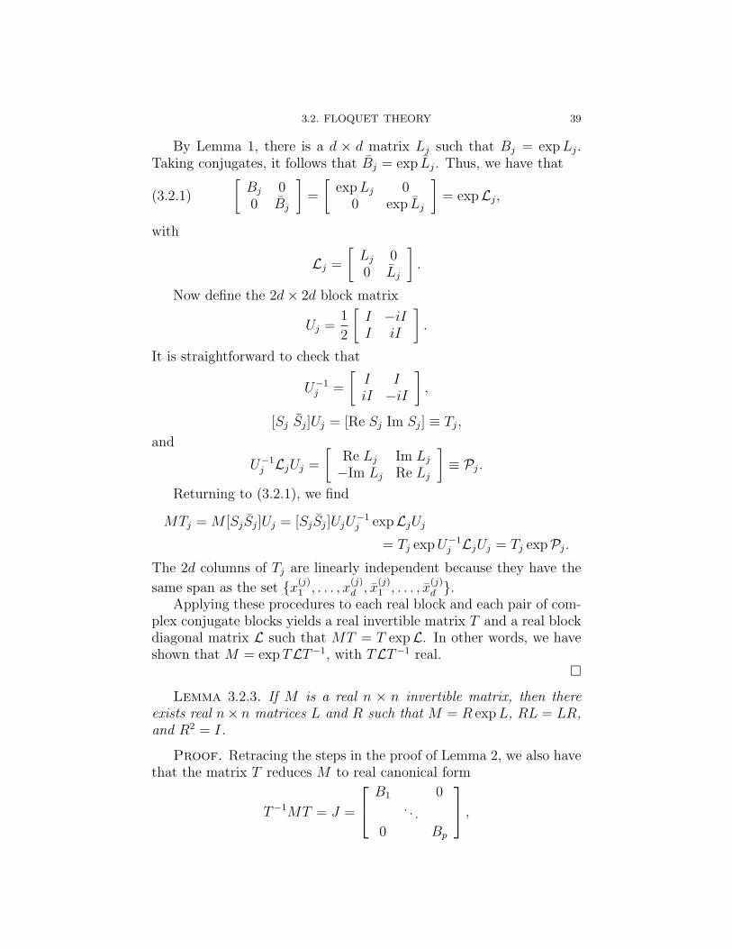
3.2. FLOQUET THEORY 39
By Lemma 1, there is a d × d matrix Lj such that Bj = expLj.Taking conjugates, it follows that Bj = exp Lj. Thus, we have that[
Bj 00 Bj
]=
[expLj 0
0 exp Lj
]= expLj,(3.2.1)
with
Lj =
[Lj 00 Lj
].
Now define the 2d× 2d block matrix
Uj =1
2
[I −iII iI
].
It is straightforward to check that
U−1j =
[I IiI −iI
],
[Sj Sj]Uj = [Re Sj Im Sj] ≡ Tj,
and
U−1j LjUj =
[Re Lj Im Lj
−Im Lj Re Lj
]≡ Pj.
Returning to (3.2.1), we find
MTj = M [SjSj]Uj = [SjSj]UjU−1j expLjUj
= Tj expU−1j LjUj = Tj expPj.
The 2d columns of Tj are linearly independent because they have the
same span as the set x(j)1 , . . . , x
(j)d , x
(j)1 , . . . , x
(j)d .
Applying these procedures to each real block and each pair of com-plex conjugate blocks yields a real invertible matrix T and a real blockdiagonal matrix L such that MT = T expL. In other words, we haveshown that M = expTLT−1, with TLT−1 real.
Lemma 3.2.3. If M is a real n × n invertible matrix, then thereexists real n× n matrices L and R such that M = R expL, RL = LR,and R2 = I.
Proof. Retracing the steps in the proof of Lemma 2, we also havethat the matrix T reduces M to real canonical form
T−1MT = J =
B1 0. . .
0 Bp
,
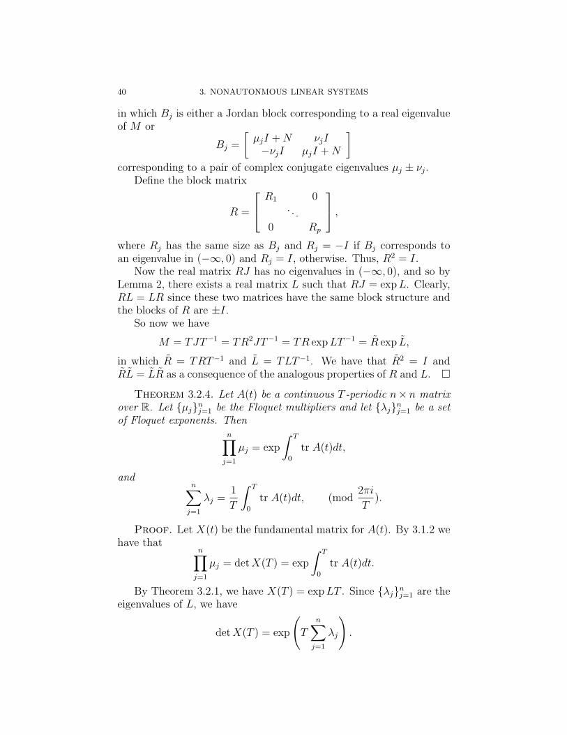
40 3. NONAUTONMOUS LINEAR SYSTEMS
in which Bj is either a Jordan block corresponding to a real eigenvalueof M or
Bj =
[µjI +N νjI−νjI µjI +N
]corresponding to a pair of complex conjugate eigenvalues µj ± νj.
Define the block matrix
R =
R1 0. . .
0 Rp
,where Rj has the same size as Bj and Rj = −I if Bj corresponds toan eigenvalue in (−∞, 0) and Rj = I, otherwise. Thus, R2 = I.
Now the real matrix RJ has no eigenvalues in (−∞, 0), and so byLemma 2, there exists a real matrix L such that RJ = expL. Clearly,RL = LR since these two matrices have the same block structure andthe blocks of R are ±I.
So now we have
M = TJT−1 = TR2JT−1 = TR expLT−1 = R exp L,
in which R = TRT−1 and L = TLT−1. We have that R2 = I andRL = LR as a consequence of the analogous properties of R and L.
Theorem 3.2.4. Let A(t) be a continuous T -periodic n× n matrixover R. Let µjn
j=1 be the Floquet multipliers and let λjnj=1 be a set
of Floquet exponents. Thenn∏
j=1
µj = exp
∫ T
0
tr A(t)dt,
andn∑
j=1
λj =1
T
∫ T
0
tr A(t)dt, (mod2πi
T).
Proof. Let X(t) be the fundamental matrix for A(t). By 3.1.2 wehave that
n∏j=1
µj = detX(T ) = exp
∫ T
0
tr A(t)dt.
By Theorem 3.2.1, we have X(T ) = expLT . Since λjnj=1 are the
eigenvalues of L, we have
detX(T ) = exp
(T
n∑j=1
λj
).
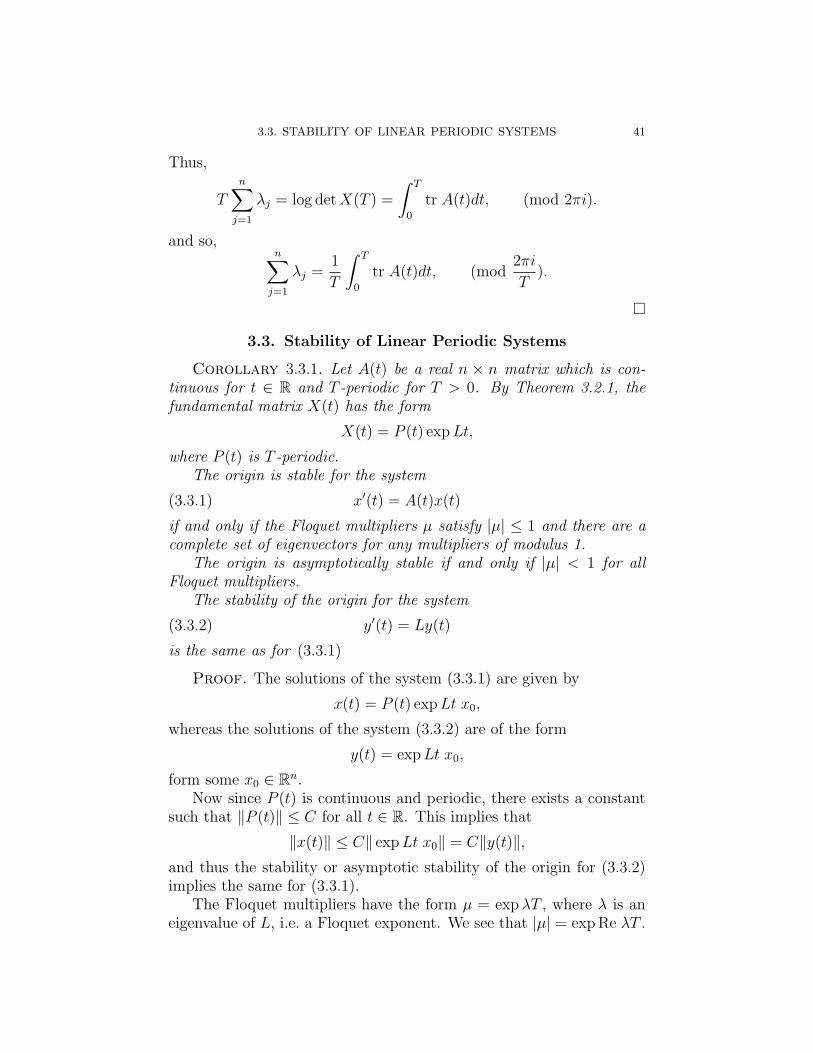
3.3. STABILITY OF LINEAR PERIODIC SYSTEMS 41
Thus,
Tn∑
j=1
λj = log detX(T ) =
∫ T
0
tr A(t)dt, (mod 2πi).
and so,n∑
j=1
λj =1
T
∫ T
0
tr A(t)dt, (mod2πi
T).
3.3. Stability of Linear Periodic Systems
Corollary 3.3.1. Let A(t) be a real n × n matrix which is con-tinuous for t ∈ R and T -periodic for T > 0. By Theorem 3.2.1, thefundamental matrix X(t) has the form
X(t) = P (t) expLt,
where P (t) is T -periodic.The origin is stable for the system
(3.3.1) x′(t) = A(t)x(t)
if and only if the Floquet multipliers µ satisfy |µ| ≤ 1 and there are acomplete set of eigenvectors for any multipliers of modulus 1.
The origin is asymptotically stable if and only if |µ| < 1 for allFloquet multipliers.
The stability of the origin for the system
(3.3.2) y′(t) = Ly(t)
is the same as for (3.3.1)
Proof. The solutions of the system (3.3.1) are given by
x(t) = P (t) expLt x0,
whereas the solutions of the system (3.3.2) are of the form
y(t) = expLt x0,
form some x0 ∈ Rn.Now since P (t) is continuous and periodic, there exists a constant
such that ‖P (t)‖ ≤ C for all t ∈ R. This implies that
‖x(t)‖ ≤ C‖ expLt x0‖ = C‖y(t)‖,and thus the stability or asymptotic stability of the origin for (3.3.2)implies the same for (3.3.1).
The Floquet multipliers have the form µ = expλT , where λ is aneigenvalue of L, i.e. a Floquet exponent. We see that |µ| = exp Re λT .
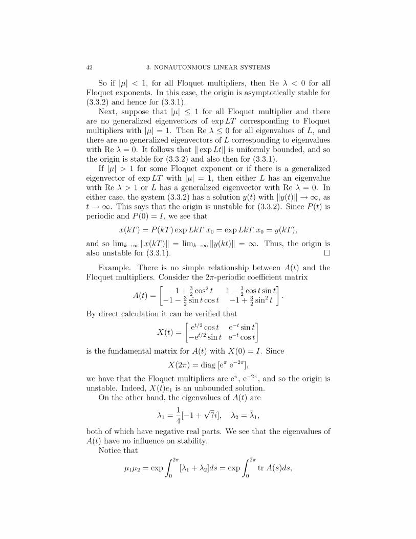
42 3. NONAUTONMOUS LINEAR SYSTEMS
So if |µ| < 1, for all Floquet multipliers, then Re λ < 0 for allFloquet exponents. In this case, the origin is asymptotically stable for(3.3.2) and hence for (3.3.1).
Next, suppose that |µ| ≤ 1 for all Floquet multiplier and thereare no generalized eigenvectors of expLT corresponding to Floquetmultipliers with |µ| = 1. Then Re λ ≤ 0 for all eigenvalues of L, andthere are no generalized eigenvectors of L corresponding to eigenvalueswith Re λ = 0. It follows that ‖ expLt‖ is uniformly bounded, and sothe origin is stable for (3.3.2) and also then for (3.3.1).
If |µ| > 1 for some Floquet exponent or if there is a generalizedeigenvector of expLT with |µ| = 1, then either L has an eigenvaluewith Re λ > 1 or L has a generalized eigenvector with Re λ = 0. Ineither case, the system (3.3.2) has a solution y(t) with ‖y(t)‖ → ∞, ast→∞. This says that the origin is unstable for (3.3.2). Since P (t) isperiodic and P (0) = I, we see that
x(kT ) = P (kT ) expLkT x0 = expLkT x0 = y(kT ),
and so limk→∞ ‖x(kT )‖ = limk→∞ ‖y(kt)‖ = ∞. Thus, the origin isalso unstable for (3.3.1).
Example. There is no simple relationship between A(t) and theFloquet multipliers. Consider the 2π-periodic coefficient matrix
A(t) =
[−1 + 3
2cos2 t 1− 3
2cos t sin t
−1− 32sin t cos t −1 + 3
2sin2 t
].
By direct calculation it can be verified that
X(t) =
[et/2 cos t e−t sin t−et/2 sin t e−t cos t
]is the fundamental matrix for A(t) with X(0) = I. Since
X(2π) = diag [eπ e−2π],
we have that the Floquet multipliers are eπ, e−2π, and so the origin isunstable. Indeed, X(t)e1 is an unbounded solution.
On the other hand, the eigenvalues of A(t) are
λ1 =1
4[−1 +
√7i], λ2 = λ1,
both of which have negative real parts. We see that the eigenvalues ofA(t) have no influence on stability.
Notice that
µ1µ2 = exp
∫ 2π
0
[λ1 + λ2]ds = exp
∫ 2π
0
tr A(s)ds,
3.4. PARAMETRIC RESONANCE – THE MATHIEU EQUATION 43
which confirms Theorem 3.2.4.
3.4. Parametric Resonance – The Mathieu Equation
The Mathieu equation is
u′′ + (ω2 + ε cos t)u = 0.
With x(t) = [u(t) u′(t)]T and
A(t) =
[0 1
−(ω2 + ε cos t) 0
]the equation can be written as a first order system
x′(t) = A(t)x(t).
Notice that A(t) is 2π-periodic, and so Floquet theory applies.
Question: For which values of ω and ε is the zero solution stable?
Corollary 3.3.1 tells us to look at the Floquet multipliers in orderto answer this question. In this case, the Floquet multipliers are theeigenvalues of X(2π), where X(t) = X(t, 0) is the fundamental matrixfor A(t).
Since tr A(t) = 0 for every t ∈ R, We have from Theorem 3.2.4that the Floquet multipliers µ1, µ2 satisfy
µ1µ2 = detX(t) = 1, t ∈ R.
If µ1 /∈ R, then µ1 = µ2. It follows that µ1, µ2 are distinct pointson the unit circle, and so there are no generalized eigenvectors. ByCorollary 3.3.1, the origin is stable.
When ε = 0, the system reduces to a harmonic oscillator. Thefundamental matrix for this constant coefficient system is
X(t) =
[cosωt −ω−1sinωtω sinωt cosωt
],
The Floquet multipliers are the eigenvalues of X(2π). They satisfyµ1 + µ2 = tr X(2π) = 2 cos 2πω. Since µ1µ2 = 1, we have that µj ∈ Rif and only if µ1 + µ2 = ±2. This can happen if and only if 2ω ∈ Z.
If 2ω /∈ Z, then by continuous dependence on parameters (to bediscussed, see Theorem 5.2.1), the Floquet multipiers will not be realfor ε small. Thus, for every 2πω0 /∈ Z, there is a small ball in the(ω, ε) plane with center (ω0, 0) where the origin is stable for Mathieu’sequation.
44 3. NONAUTONMOUS LINEAR SYSTEMS
It can also be shown, although we will not do so now, that there areregions of instability branching off of the points (ω0, 0) when 2πω0 ∈ Z.This is the so-called parametric resonance.
3.5. Existence of Periodic Solutions
Theorem 3.5.1. Let A(t) be T -periodic. The system x′(t) = A(t)x(t)has a nonzero T -periodic solution if and only if A(t) has the Floquetmultiplier µ = 1.
Proof. By the periodicity of A(t) and uniqueness, we have that asolution is T -periodic if and only if
(3.5.1) x(T ) = x(0).
Let X(t) be the fundamental matrix for A(t) with X(0) = I. Thenevery nonzero solution has the form x(t) = X(t)x0 for some x0 ∈ Rn
with x0 6= 0. It follows that (3.5.1) holds if and only if X(T )x0 =x0. Thus, x0 is an eigenvector for X(T ) with eigenvalue 1. But theeigenvalues of X(T ) are the Floquet multipliers.
Theorem 3.5.2. Let A(t) be a continuous n × n matrix and letF (t) be a continuous vector in Rn. Assume that A(t) and F (t) areT -periodic. The equation
(3.5.2) x′(t) = A(t)x(t) + F (t)
has a T -periodic solution if and only if
(3.5.3)
∫ T
0
y(t) · F (t)dt = 0,
for all T -periodic solutions y(t) of the adjoint system
(3.5.4) y′(t) = −A(t)Ty(t).
Proof. Let X(t) = X(t, 0) be the fundamental matrix for A(t)with X(0) = I. By variation of parameters, we have that the solutionx(t) = x(t, 0, x0) of (3.5.2) is given by
x(t) = X(t)x0 +X(t)
∫ t
0
X(s)−1F (s)ds.
By uniqueness and periodicity, x(t) is T -periodic if and only ifx(T ) = x(0) = x0. This is equivalent to
[I −X(T )]x0 = X(T )
∫ T
0
X(s)−1F (s)ds,
3.5. EXISTENCE OF PERIODIC SOLUTIONS 45
and so, multiplying both sides by X(T )−1, we obtain an equivalentlinear system of equations
(3.5.5) Bx0 = g,
in which
B = X(T )−1 − I and g =
∫ T
0
X(s)−1F (s)ds.
Thus, x(t, 0, x0) is a T -periodic solution (3.5.2) if and only if x0 isa solution of (3.5.5).
By the Fredholm Alternative 4.2.1 (to follow), the system (3.5.5)has a solution if and only if g · y0 = 0 for all y0 ∈ N(BT ).
We now characterize N(BT ). Let Y (t) = Y (t, 0) be the fundamen-tal matrix for −A(t)T . Then Y (t) = [X(t)−1]T , so
BT = Y (T )− I.
Thus, y0 ∈ N(BT ) if and only if y0 = Y (T )y0. This, in turn, isequivalent to saying y0 ∈ N(BT ) if and only if y(t) = Y (t)y0 is aT -periodic solution of the adjoint system (3.5.4).
Now we examine the orthogonality condition. We have
y0 · g =
∫ T
0
y0 ·X(s)−1F (s)ds
=
∫ T
0
y0 · Y (s)TF (s)ds
=
∫ T
0
Y (s)y0 · F (s)ds
=
∫ T
0
y(s) · F (s)ds.
The result now follows from the following chain of equivalent state-ments: Equation (3.5.2) has a T -periodic solution iff the system (3.5.5)has a solution iff y0 · g = for every y0 ∈ N(BT ) iff (3.5.3) holds forevery T -periodic solution of (3.5.4).
Remark: Theorem 3.5.2 is interesting only when F 6= 0, becausethe conditions (3.5.3), (3.5.4) hold trivially when F = 0 and the trivialx = 0 is T -period.
Example. Consider the periodically forced harmonic oscillator:
u′′ + u = cosωt, ω > 0.
This is equivalent to the first order system
(3.5.6) x′(t) = Ax(t) + F (t)
46 3. NONAUTONMOUS LINEAR SYSTEMS
with
x(t) =
[u(t)u′(t)
], A =
[0 1−1 0
], F (t) =
[0
cosωt
].
Notice that F (t) (and A) are T -periodic with T = 2π/ω.Since −AT = A, the adjoint equation is
y′ = Ay,
the solutions of which are
y(t) = expAt y0, with expAt =
[cos t sin t− sin t cos t
].
All solutions of the adjoint equation are 2π-periodic.If the forcing frequency ω satisfies ω 6= 1, then the adjoint equation
has no T -periodic solutions. Thus, the system (3.5.6) has a T -periodicsolution. This solution is, in fact, unique because the system (3.5.5)which determines its initial data has a unique solution (the 2×2 matrixB is onto and hence one-to-one).
If ω = 1, then T = 2π, and there are no 2π-periodic solutions of(3.5.6), since there exist 2π-periodic solutions of the adjoint equationfor which the orthogonality condition (3.5.3) does not hold. Here is thecalculation:∫ T
0
y(s) · F (s)ds =
∫ T
0
expAs y0 · F (s)ds
=
∫ T
0
y0 · [expAs]TF (s)ds
=
∫ T
0
y0 · [− sin s cos s e1 + cos2 s e2]ds
= π y0 · e2.This is nonzero for y0 · e2 6= 0. This is the case of resonance.
This overly simple example can be solved explicitly, since A is con-stant. However, the example illustrates the use of the Fredholm alter-native in such problems.
CHAPTER 4
Results from Functional Analysis
4.1. Operators on Banach Space
Definition 4.1.1. A Banach space is a complete normed vectorspace over R or C.
A Hilbert space is a Banach space whose norm is induced by aninner product.
Here are some examples of Banach spaces that will be relevant forus:
- Let F ⊂ Rn. C0(F ,Rm) is set the of continuous functionsfrom F into Rm. Define the norm
‖f‖C0 = supx∈F
‖f(x)‖.
Then
C0b (F ,Rm) = f ∈ C0(F ,Rm) : ‖f‖C0 <∞,
is a Banach space. If F is compact, then C0b (F ,Rm) = C0(F ,Rm).
- C1(F ,Rm) is set the of functions f from F into Rm such thatDf(x) exists and is continuous. Define the norm
‖f‖C1 = supx∈F
‖f(x)‖+ supx∈F
‖Df(x)‖.
Then
C1b (F ,Rm) = f ∈ C1(F ,Rm) : ‖f‖C1 <∞,
is a Banach space.- Lip(F ,Rm) is the set of Lipschitz continuous functions from F
into Rm such that the norm
‖f‖Lip = supx∈F
‖f(x)‖+ supx,y∈Fx6=y
‖f(x)− f(y)‖‖x− y‖
is finite.
Notice that C1b (F ,Rm) ⊂ Lip(F ,Rm) ⊂ C0
b (F ,Rm).
47
48 4. RESULTS FROM FUNCTIONAL ANALYSIS
Definition 4.1.2. Let X and Y be Banach spaces. Let A : X → Ybe a linear operator. A is bounded if and only if
sup‖x‖X 6=0
‖Ax‖Y
‖x‖X
≡ ‖A‖X,Y <∞.
‖A‖X,Y is the operator norm.
The set of all bounded linear operators from X to Y is denoted byL(X,Y ). It is a Banach space with the operator norm.
A linear operator from X to Y is bounded if and only if it is con-tinuous.
Definition 4.1.3. Let f : X → Y be any mapping between theBanach spaces X and Y . (f is not necessarily linear.) f is Frechetdifferentiable at a point x0 ∈ X if and only if there exists a linearoperator Df(x0) ∈ L(X, Y ) such that
f(x)− f(x0)−Df(x0)(x− x0) ≡ R(x, x0)
satisfies
limx→x0
‖R(x, x0)‖Y
‖x− x0‖X
= 0.
(Dxf(x0) is unique if it exists.)Let U ⊂ X be an open set. We say that f : X → Y is differentiable
on U if and only if Dxf(x) exists for all x ∈ U .f is continuously differentiable on U if and only if it is differentiable
on U and Dxf(x) is a continuous map from X into L(X, Y ).
Remark: The Frechet derivative can be computed as follows
Df(x0)x = limε→0
ε−1[f(x0 + εx)− f(x0)] = Dεf(x0 + εx)|ε=0.
Example: Let X = C0([0, 1],R). Given f ∈ X, define the nonlinearmapping
T (f)(t) =
∫ t
0
[f(s)]2ds.
Then T : X → X. In fact, T is differentiable, and given f0, f ∈ X, wehave that DT (f0)f is the function whose value at a point t ∈ [0, 1] is
DT (f0)f(t) = 2
∫ t
0
f0(s)f(s)ds.
4.2. THE FREDHOLM ALTERNATIVE 49
4.2. The Fredholm Alternative
Theorem 4.2.1 (Fredholm Alternative). Let Hi, i = 1, 2 be Hilbertspaces with inner product 〈·, ·〉i. Let A : H1 → H2 be a bound linearoperator, and let A∗ : H2 → H1 be its adjoint. Then R(A) = N(A∗)⊥.
Proof. Let f ∈ R(A). Then f = Ax, for some x ∈ H1. For anyy ∈ N(A∗), we have
〈f, y〉2 = 〈Ax, y〉2 = 〈x,A∗y〉1 = 0.
Thus, f ∈ N(A∗)⊥. This shows that
(4.2.1) R(A) ⊂ N(A∗)⊥.
Write H2 = N(A∗) ⊕ N(A∗)⊥ (orthogonal direct sum). The sub-space N(A∗) is closed and
A∗ : N(A∗)⊥ → R(A∗)
is one-to-one and onto. The subspace R(A∗) is closed by the ClosedGraph Theorem. But then also by the Closed Graph Theorem,
A∗−1 : R(A∗) → N(A∗)⊥
is bounded.Let g ∈ N(A∗)⊥. Define the bounded linear functional
φ(z) = 〈g, A∗−1z〉2
on the Hilbert space R(A∗). By the Riesz representation theorem, thereis a unique x ∈ R(A∗) such that
〈g, A∗−1z〉2 = 〈x, z〉1,
for all z ∈ R(A∗). Thus, given any y ∈ N(A∗)⊥, we may write y = A∗z,for some z ∈ R(A∗) and
〈g, y〉2 = 〈g, A∗z〉2 = 〈x, z〉1 = 〈x,A∗y〉1.
Thus, we have that
〈g − Ax, y〉2 = 0,
for all y ∈ N(A∗)⊥. Now by (4.2.1), we have that Ax ∈ N(A∗)⊥.So since g ∈ N(A∗)⊥, we have that g − Ax ∈ N(A∗)⊥. Taking y =g−Ax, we see that g−Ax = 0, and thus, g ∈ R(A). This proves thatN(A∗)⊥ ⊂ R(A).
50 4. RESULTS FROM FUNCTIONAL ANALYSIS
4.3. The Contraction Mapping Principle in Banach Space
Let X be a Banach space. If we define the distance between twopoints x and y in X to be d(x, y) = ‖x − y‖X , then X is a completemetric space. Any closed subset of X is also a complete metric space.In this context, the contraction mapping principle says:
Theorem 4.3.1 (Contraction mapping principle in Banach space).Let V ⊂ X be a closed subset. Let T : V → V be a contractionmapping, i.e. there exists a constant 0 < α < 1 such that
‖T (x)− T (y)‖X ≤ α‖x− y‖X ,
for all x, y ∈ V . Then T has a unique fixed point x ∈ V , i.e. T (x) = x.
Proof. The set V is closed, so (V, d) is a complete metric space.Apply the standard contraction mapping principle.
We want to generalize this result to the situation where the map-ping, and hence the corresponding fixed points, depends on parameters.
Definition 4.3.1. Let X and Y be Banach spaces. Let U ⊂ X andV ⊂ Y be open sets. A mapping T : U × V → V is called a uniformcontraction if there is a constant 0 < α < 1 such that
‖T (x, y1)− T (x, y2)‖Y ≤ α‖y1 − y2‖Y ,
for all x ∈ U and y1, y2 ∈ V . Notice that the contraction number α isuniform for x throughout U .
An application of the contraction mapping principle shows that ifT : U × V → V is a uniform contraction, then for every x ∈ U there isa unique fixed point g(x) ∈ V , i.e. a unique solution of the equation
T (x, g(x)) = g(x).
The following result shows that if the mapping T is continuous ordifferentiable then the fixed point g(x) depends continuously or differ-entiably on x.
Theorem 4.3.2 (Uniform Contraction Principle). Let T be a uni-form contraction, and let g : U → V be the corresponding fixed point.If T ∈ Ck(U × V , Y ) for k = 0 or 1, then g ∈ Ck(U, Y ).
4.3. THE CONTRACTION MAPPING PRINCIPLE IN BANACH SPACE 51
Proof. The case k = 0 is easy. By the definition of g, the triangleinequality, and the uniform contraction hypothesis, we have
‖g(x+ h)− g(x)‖ = ‖T (x+ h, g(x+ h))− T (x, g(x))‖≤ ‖T (x+ h, g(x+ h))− T (x+ h, g(x))‖
+ ‖T (x+ h, g(x))− T (x, g(x))‖≤ α‖g(x+ h)− g(x)‖
+ ‖T (x+ h, g(x))− T (x, g(x))‖.Thus, since α < 1, we get
‖g(x+ h)− g(x)‖ ≤ 1
1− α‖T (x+ h, g(x))− T (x, g(x))‖.
But T is assumed to be continuous, so
limh→0
‖g(x+ h)− g(x)‖ = 0,
i.e. g is continuous at x.Let’s first look at the strategy for the case k = 1. Since T (x, g(x)) =
g(x), we would have if g were C1 (remember that this is what we’retrying to prove)
DxT (x, g(x)) +DyT (x, g(x))Dxg(x) = Dxg(x).
Here, DxT = DT |X×0 and DyT = DT |0×Y . This inspires us toconsider the operator equation
(4.3.1) DxT (x, g(x)) +DyT (x, g(x))M(x) = M(x).
We will first show that we can solve this for M(x) ∈ L(X,Y ), and thenwe will show that M(x) = Dxg(x).
T is assumed to be C1, so for each (x, y) ∈ U × V , DyT (x, y) ∈L(Y, Y ). Since T is a uniform contraction, it can easily be shown that‖DyT (x, y)‖ ≤ α < 1. It follows that I − DyT (x, g(x)) is invertiblefor all x ∈ U , its inverse depends continuously on x, and the inverse isbounded by 1/(1− α). Thus, the solution of(4.3.1) is
(4.3.2) M(x) = [I −DyT (x, g(x))]−1DxT (x, g(x)) ∈ L(X, Y ),
and M(x) depends continuously on x ∈ U .Having constructed M(x), it remains to show that M(x) = Dxg(x).
We are going to prove that
R(x, h) ≡ g(x+ h)− g(x)−M(x)h
satisfies
limh→0
‖R(x, h)‖‖h‖
= 0.
52 4. RESULTS FROM FUNCTIONAL ANALYSIS
Put γ(h) = g(x+ h)− g(x). Then
γ(h) = T (x+ h, g(x+ h))− T (x, g(x))
= T (x+ h, g(x) + γ(h))− T (x, g(x))(4.3.3)
= DxT (x, g(x))h+DyT (x, g(x))γ(h) + ∆(h, γ(h)),
in which
∆(h, γ) = T (x+ h, g(x) + γ)
− T (x, g(x))−DxT (x, g(x))h−DyT (x, g(x))γ.
Since T is C1, for any 0 < ε < (1−α)/2, there is a δ > 0 such that
‖∆(h, γ)‖ < ε(‖h‖+ ‖γ‖),
for all (h, γ) ∈ U × V with ‖h‖+ ‖γ‖ < δ.Next, since γ(h) is continuous in h and γ(0) = 0, we can find
0 < δ′ < δ/2 such that
‖γ(h)‖ < δ/2 provided that ‖h‖ < δ′.
So for ‖h‖ < δ′, we have ‖h‖+ ‖γ(h)‖ < δ/2 + δ/2 = δ.Combining the last two paragraphs, we see that if ‖h‖ < δ′, then
(4.3.4) ‖∆(h, γ(h))‖ < ε(‖h‖+ ‖γ(h)‖).
By (4.3.3), we get for all ‖h‖ < δ′,
‖γ(h)‖ ≤ ‖DxT (x, g(x))‖‖h‖+ α‖γ(h)‖+ ε(‖h‖+ ‖γ(h)‖),
or upon rearrangement,
‖γ(h)‖ ≤ 1
1− α− ε[‖DxT (x, g(x))‖‖h‖+ ε‖h‖] ≤ k‖h‖,
with k independent of ε < (1− α)/2.Therefore, going back to (4.3.4), we have that
‖∆(h, γ(h))‖ < ε(1 + k)‖h‖,
for all ‖h‖ < δ′.Now return to (4.3.3). Solving for γ(h) and inserting the definition
(4.3.2), the formula (4.3.3) can be rewritten as
γ(h) = [I −DyT (x, g(x))]−1[DxT (x, g(x))h+ ∆(h, γ(h))]
= M(x)h+ [I −DyT (x, g(x))]−1∆(h, γ(h)).
4.4. THE IMPLICIT FUNCTION THEOREM IN BANACH SPACE 53
So finally, we get
R(x, h) = ‖γ(h)−M(x)h‖≤ ‖[I −DyT (x, g(x))]−1‖‖∆(h, γ(h))‖
≤ 1
1− αε(1− k)‖h‖,
for all ‖h‖ < δ′. It follows that
limh→0
‖γ(h)−M(x)h‖‖h‖
= 0.
4.4. The Implicit Function Theorem in Banach Space
Theorem 4.4.1. Suppose that X, Y , and Z are Banach spaces.Let U ⊂ X and V ⊂ Y be open sets. Let F : U × V → Z be a C1
mapping. Assume that there exists a point (x0, y0) ∈ U × V such thatF (x0, y0) = 0 and DyF (x0, y0) has a bounded inverse in L(Z, Y ). Thenthere are a neighborhood U1×V1 ⊂ U×V of (x0, y0) and a C1 mappingg : U1 → V1 such that
y0 = g(x0) and F (x, g(x)) = 0,
for all x ∈ U1. If F (x, y) = 0 for (x, y) ∈ U1 × V1, then y = g(x).
4.4.1
Proof. Let L = DyF (x0, y0)−1, and define the C1 map G : U ×
V → Y by
G(x, y) = y − LF (x, y).
Notice that G(x, y) = y if and only if F (x, y) = 0. We also haveG(x0, y0) = y0 and DyG(x0, y0) = 0.
By continuity, given ε = 1/4 there exists a δ1 > 0 such that
‖DyG(x, y)‖ = ‖DyG(x, y)−DyG(x0, y0)‖ < 1/4,
for (x, y) ∈ N = Bδ1(x0)×Bδ1(y0). We can also find a constant M > 0such that
‖DxG(x, y)‖ ≤M,
for (x, y) ∈ N .
54 4. RESULTS FROM FUNCTIONAL ANALYSIS
Take a pair of points (xi, yi) ∈ N , i = 1, 2. Set x(s) = sx2+(1−s)x1
and y(s) = sy2 + (1− s)y1. Then
G(x2, y2)−G(x1, y1) =
∫ 1
0
d
dsG(x(s), y(s))ds
=
∫ 1
0
DxG(x(s), y(s))(x2 − x1)ds
+
∫ 1
0
DyG(x(s), y(s))(y2 − y1)ds.
So by the preceding estimates, we obtain
‖G(x2, y2)−G(x1, y1)‖ ≤M‖x2 − x1‖+ (1/4)‖y2 − y1‖.Set δ2 = minδ1, δ1/4M. Define U1 = Bδ2(x0) and V1 = Bδ1(y0).
The claim is thatG : U1×V 1 → V 1 and thatG is a uniform contraction.Let (x, y) ∈ U1 × V 1. Then
‖G(x, y)− y0‖ = ‖G(x, y)−G(x0, y0)‖≤ M‖x− x0‖+ (1/4)‖y − y0‖≤ Mδ2 + (1/4)δ1
≤ (1/4)δ1 + (1/4)δ1 = δ1/2.
Thus G(x, y) ∈ V 1.We also have for all (x, y1), (x, y2) ∈ U1 × V 1 that
‖G(x, y1)−G(x, y2)‖ ≤ (1/4)‖y1 − y2‖,which means that G is a uniform contraction.
Applying the uniform contraction principle, there is a C1 map g :U1 → V1 such that
G(x, g(x)) = g(x),
for all x ∈ U1. Moreover, given x ∈ U1, y = g(x) ∈ V1 is the uniquepoint such that G(x, y) = y.
Of course, this theorem includes the case of finite dimensions:
X = Rm, Y = Z = Rn.
CHAPTER 5
Dependence on Initial Conditions and Parameters
5.1. Smooth Dependence on Initial Conditions
We have seen in Theorem 2.5.1 that solutions of the initial valueproblem depend continuously on initial conditions. We will now showthat this dependence is as smooth as the vector field.
Theorem 5.1.1. Let Ω ⊂ Rn+1 be an open set, and suppose thatf : Ω → Rn is C1.
For (s, p) ∈ Ω, the unique local solution x(t, s, p) of the initial valueproblem
(5.1.1)d
dtx(t, s, p) = f(t, x(t, s, p)), x(s, s, p) = p.
is C1 in its open domain of definition
D = (t, s, p) ∈ Rn+2 : α(s, p) < t < β(s, p), (s, p) ∈ Ω.
The differential matrix Dpx(t, s, p) satisfies the so-called linear vari-ational equation
d
dtDpx(t, s, p) = Dxf(t, x(t, s, p))Dpx(t, s, p),
(5.1.2)
Dpx(s, s, p) = I.
Also,
(5.1.3)∂x
∂s(t, s, p) = −Dpx(t, s, p)f(s, p).
Proof. Suppose, temporarily, that we have shown that x(t, s, p) ∈C1(D).
Then (5.1.2) follows immediately by taking the derivative of (5.1.1)with respect to p.
Next, use the properties of the flow to write
x(t, s, p) = x(t, τ, x(τ, s, p)) t, τ ∈ I(s, p).55
56 5. DEPENDENCE ON INITIAL CONDITIONS AND PARAMETERS
Take the derivative of this with respect to τ to get
0 =∂x
∂s(t, τ, x(τ, s, p)) +Dpx(t, τ, x(τ, s, p))
∂x
∂t(τ, s, p).
From this and the ODE (5.1.1), we obtain
∂x
∂s(t, τ, x(τ, s, p)) = −Dpx(t, τ, x(τ, s, p))f(τ, x(τ, s, p)).
Equation (5.1.3) follows by letting τ = s.Since we already know that the solution is continuously differ-
entiable in t, we must only establish continuous differentiability ofx(t, s, p) in (s, p). We are going to do this by a uniqueness argument.The flow x(t, s, p) satisfies the standard integral equation. We willshow that the implicit function guarantees this equation has a uniqueC1 solution. We now proceed to set this up precisely.
For an arbitrary point (s0, p0) ∈ Ω, let x0(t) = x(t, s0, p0) be thecorresponding solution to the initial value problem (5.1.1), defined onthe maximal interval I(s0, p0) = (α(s0, p0), β(s0, p0)). Choose an arbi-trary closed interval J = [a, b] with
α(s0, p0) < a < s0 < b < β(s0, p0).
Define the compact set
K = (t, x(t, s0, p0)) ∈ Ω : t ∈ J.
By the Covering Lemma 2.3.2, there exist numbers δ, ρ > 0 and acompact set K ′ ⊂ Ω such that for every (s, p) ∈ K, the cylinder
C(s, p) = (s′, p′) ∈ Rn+1 : |s′ − s| ≤ δ, ‖p′ − p‖ ≤ ρ
satisfies
C(s, p) ⊂ K ′.
Define the Banach spaces X = Rn+1 and Y = Z = C(J,Rn) withthe sup norm. Let U = (a, b)× Rn and
V = x ∈ Y : ‖x− x0‖ = supJ‖x(t)− x0(t)‖ < ρ.
We have that U ⊂ X and V ⊂ Y are open.Suppose that x ∈ V . Then for any σ ∈ J , we have that
‖x(σ)− x0(σ)‖ < ρ,
and so, (σ, x(σ)) ∈ C(σ, x0(σ)) ⊂ Ω, for any σ ∈ J . Therefore, theoperator
T : U × V → Z
5.1. SMOOTH DEPENDENCE ON INITIAL CONDITIONS 57
given by
(s, p, x) 7→ T (s, p, x)(t) = x(t)− p−∫ t
s
f(σ, x(σ))dσ, t ∈ J,
is well-defined. It is straight-forward to verify that T is C1. In partic-ular, we have that DxT (s, p, x) is linear map from Y to Z(= Y ) whichtakes y ∈ Y to the function DxT (s, p, x)[y] ∈ Z whose value at a pointt ∈ J is
DxT (s, p, x)[y](t) = y(t)−∫ t
s
A(σ)y(σ)dσ with A(σ) = Dxf(σ, x(σ)).
(It is here that we are using the assumption f ∈ C1(Ω).)Since x0(t) = x(t, s0, p0) solves (5.1.1) we have that
T (s0, p0, x0) = 0.
Now we claim that DxT (s0, p0, x0) is invertible as a linear map fromY to Z. Let g ∈ Z. The equation DxT (s0, p0, x0)[y] = g can be writtenexplictly as
(5.1.4) y(t)−∫ t
s0
A(σ)y(σ)dσ = g(t).
Letting u(t) = y(t)− g(t), this is equivalent to
u(t) =
∫ t
s0
A(σ)[u(σ) + g(σ)]dσ.
Notice that the right-hand side is C1 in t. So this is equivalent to
u′(t) = A(t)[u(t) + g(t)], t ∈ J, u(s0) = 0.
We can represent the unique solution of this initial value problem usingthe variation of parameters formula. Let W (t, s) be the fundamentalmatrix for A(t). Then
u(t) =
∫ t
s0
W (t, σ)A(σ)g(σ)dσ.
Since u = y − g, this is equivalent to
(5.1.5) y(t) = g(t) +
∫ t
s0
W (t, σ)A(σ)g(σ)dσ.
We have shown that for every g ∈ Z, the equation (5.1.4) has aunique solution y ∈ Y given by (5.1.5). This proves the invertibil-ity of DxT (s0, p0, x0). Finally, from the formula (5.1.5), we see thatthe inverse is a bounded map from Z to Y .
58 5. DEPENDENCE ON INITIAL CONDITIONS AND PARAMETERS
By the Implicit Function Theorem 4.4.1, there are a neighborhoodU0 ⊂ U of (s0, p0), a neighborhood V0 ⊂ V of x0, and a C1 mapφ : U0 → V0 such that φ(s0, p0) = x0 and T (s, p, φ(s, p)) = 0 for all(s, p) ∈ U0. Furthermore, if (s, p, x) ∈ U0 × V0 is a point such thatT (s, p, x) = 0, then x = φ(s, p).
Since the map (s, p) 7→ φ(s, p) is C1 from U0 into V0 ⊂ Y , it followsthat the function φ(s, p)(t) is C1 in (s, p) for all t ∈ J .
By continuous dependence on initial conditions, Theorem (2.5.1),there is a neighborhood N of (s0, p0) such that for all (s, p) ∈ N , wehave that
J ⊂ I(s, p), and ‖x(t, s, p)− x(t, s0, p0)‖ < ρ, for all t ∈ J.Therefore, for all (s, p) ∈ N , we have that x(t, s, p) ∈ V0. Since x(t, s, p)solves the initial value problem, we also have that T (s, p, x(·, s, p)) = 0.
By the uniqueness portion of the implicit function theorem, weconclude that
x(t, s, p) = φ(s, p)(t), for all (s, p) ∈ U0 ∩N, t ∈ J.Therefore, x(t, s, p) is C1 on J×(U0∩N). Since, (s0, p0) is an arbitrarypoint in Ω, and J is an arbitrary subinterval of I(s0, p0), it follows thatx(t, s, p) is C1 on all of D.
Corollary 5.1.1. If f(t, x) is continuous on Ω ⊂ Rn+1 and Ck inx, then x(t, s, p) is Ck in (s, p) on its open domain of definition. (Iff(t, x) is in Ck(Ω), then x(t, s, p) is Ck in (t, s, p) on its domain ofdefinition.)
This is proved by induction on k. The corollary can be proved fork = m+ 1, by applying the result for k = m to the ODE’s satisfied bythe first derivatives of x(t, s, p). The first derivatives of x(t, s, p) in Cm
implies that x(t, s, p) is in Cm+1.
Corollary 5.1.2.
detDpx(t, s, p) = exp
∫ t
s
n∑j=1
∂fj
∂xj
(τ, x(τ, s, p))dτ.
Proof: This follows by applying Theorem 3.1.2 to the variational equa-tion:
d
dtDpx(t, s, p) = Dxf(t, x(t, s, p))Dpx(t, s, p),
and noting that
tr Dxf =n∑
j=1
∂fj
∂xj
.
5.2. CONTINUOUS DEPENDENCE ON PARAMETERS 59
5.2. Continuous Dependence on Parameters
Theorem 5.2.1. Let f(t, x, λ) be continuous on an open set Ω ⊂Rn+1×Rm with values in Rn. Assume that f(t, x, λ) is locally Lipschitzwith respect to (x, λ). Then given (t0, x0, λ) ∈ Ω, the initial valueproblem
x′ = f(t, x, λ), x(t0) = x0
has a unique local solution x(t, t0, x0, λ) on a maximal interval of defi-nition
I(t0, x0, λ) = (α(t0, x0, λ), β(t0, x0, λ))
where
(i) α(t0, x0, λ) is upper semi-continuous.(ii) β(t0, x0, λ) is lower semi-continuous.(iii) x(t, t0, x0, λ) is continuous on its open domain of definition
(t, t0, x0, λ) : t ∈ I(t0, x0, λ); (t0, x0, λ) ∈ Ω.
Proof: Here’s the trick: turn the parameter λ into a dependent variableand use the old continuous dependence result, Theorem 2.5.1. Definea new vector
y =
[xλ
]∈ Rn × Rm,
and a new vector field
F (t, y) =
[f(t, x, λ)
0
],
on Ω. Apply the result on continuous dependence to the so-calledsuspended system
y′ = F (t, y), y(t0) = y0 =
[x0
λ0
].
Since the vector field F is 0 in its last m components, the last mcomponents of y are constant and, hence, equal to λ0. Extraction ofthe first n components yields the desired result for x(t, t0, x0, λ0).
Remark: This result is still true even if f(t, x, λ) is not locally Lipschitzcontinuous in λ, however the easy proof no longer works.
Corollary 5.2.1. If f(t, x, λ) is in Ck(Ω), then x(t, t0, x0, λ) is inCk on its open domain of definition.
Proof: Use the trick above, and then apply the result on smooth de-pendence.

CHAPTER 6
Linearization and Invariant Manifolds
6.1. Autonomous Flow At Regular Points
Last changed 01.28.10
Definition 6.1.1. For j = 1, 2, let
fj : Oj → Rn,
be C1 autonomous vector fields, with Oj ⊂ Rn open. Let φ(j)t , j = 1, 2
be the associated flows. We say that the two flows φ(1)t and φ
(2)t are
topologically conjugate if there exists a homeomorphism η : O1 → O2
such that η φ(1) = φ(2)t η.
If the map η can be chosen to be a diffeomorphism, then we will saythat the flows are diffeomorphically conjugate.
If φ(1)t and φ
(2)t are conjugate, then the maximal interval of existence
of φ(1)t (p) is the same as for φ
(2)t (η(p)), for every p ∈ O1.
Conjugacy is an equivalence relation.
Theorem 6.1.1. Two flows φ(1)t and φ
(2)t are diffeomorphically con-
jugate under η:
(6.1.1) η(φ(1)t (p)) = φ
(2)t (η(p)), p ∈ O1,
if and only if the associated vector fields satisfy
(6.1.2) Dη(p)f1(p) = f2(η(p)), p ∈ O1.
Proof. We are given that
d
dtφ
(j)t (p) = fj(φ
(j)t (p)), φ(j)(p)|t=0 = p,
for every p ∈ Oj, j = 1, 2.By the chain rule, we have that
d
dtη(φ
(1)t (p)) = Dη((φ
(1)t (p))
d
dtφ
(1)t (p)(6.1.3)
= Dη((φ(1)t (p))f1(φ
(1)t (p)).
61
62 6. LINEARIZATION AND INVARIANT MANIFOLDS
So if (6.1.2) holds, then
d
dtη(φ
(1)t (p)) = f2(η(φ
(1)t (p))).
Since η(φ(1)t (p))|t=0 = η(p), we have by uniqueness that (6.1.1) is true.
On the other hand, if (6.1.1) holds, then take the derivative in tand apply (6.1.3) to get,
Dη((φ(1)t (p))f1(φ
(1)t (p)) =
d
dtη(φ
(1)t (p)) =
d
dtφ
(2)t (η(p)) = f2(φ
(2)t (η(p))).
Setting t = 0, we recover (6.1.2).
Definition 6.1.2. A point x ∈ O is a regular point if for a vectorfield f if f(x) 6= 0.
Definition 6.1.3. An n − 1 dimensional hyperplane in Rn is asubset H ⊂ Rn of the form H = x0 + S where x0 ∈ Rn and S is ann− 1 dimensional subspace of Rn.
Since an n− 1 dimensional subspace of Rn can always be expressedin the form S = x ∈ Rn : x · ξ = 0 for some fixed nonzero vectorξ ∈ Rn, we have H = x ∈ Rn : (x − x0) · ξ = 0. The vector ξis unique up to a scalar multiple. A hyperplane divides Rn into twodisjoint sets. Given a choice of the vector ξ, we can describe themas the positive side P = x ∈ Rn : x · ξ > 0 and the negative sideN = x ∈ Rn : x · ξ < 0.
Note that if H = x0 + S is a hyperplane, then H = x + S for anyx ∈ H.
Definition 6.1.4. Let H be a hyperplane. A transversal to f is aconnected set of the form T = H ∩ U , U ⊂ O open, with the propertythat f(x) /∈ S for all x ∈ T .
Note that if T is a transversal, then f(x) 6= 0 on T , i.e. T containsonly regular points. Conversely, if x0 is a regular point, then f has atransversal at x0. (Exercise)
If T ⊂ H = x0 + S and S = x · ξ = 0, then f(x) · ξ 6= 0 on T .Since T is connected, either f(x) · ξ > 0 or f(x) · ξ < 0, for all x ∈ T .Thus, f(x) ∈ P or f(x) ∈ N , for all x ∈ T . In words, along T , f(x)points to the same side of T .
The next result shows that a smooth vector field can be transformedto a constant vector, at a regular point. The situation near a criticalpoint is more complicated and will be taken up in the next sectionwhen we come to the Hartman-Grobman theorem.
6.1. AUTONOMOUS FLOW AT REGULAR POINTS 63
Theorem 6.1.2. Let x0 ∈ O be a regular point for the vector fieldf(x). Let T ⊂ H = x0 + S be a transversal at x0. Then there existsa neighborhood U ⊂ O of x0 which is diffeomorphic to a neighborhoodof (0, 0) ∈ R × Rn−1 of the form I × V , in which I = (−ε, ε). Thediffeomorphism η has the following properties:
η : I × V → U, η(0, 0) = x0, η : 0 × V = T ∩ U,and the image of the vector field f(x) under ψ = η−1 is a constantvector:
g(ψ(x)) = Dxψ(x)f(x) = e1.
Proof. Choose vectors ξ1, . . . , ξn−1 ∈ Rn which span the subspaceS. For y = (y1, . . . , yn−1) ∈ Rn−1, define the linear combination
p(y) = x0 +n−1∑i=1
yiξi.
Then p : Rn−1 → H.Now for any y ∈ Rn−1 such that p(y) ∈ O, the existence theorem
allows us to define
η(t, y) = x(t, p(y)) for α(p(y)) < t < β(p(y)).
Since the vector field f(x) is C1, the theorem on smooth dependence(Theorem 5.1.1) ensures us that η(t, y) is a C1 function on its opendomain of definition. Notice that η(0, 0) = x(0, p(0)) = x(0, x0) = x0
and that η(0, y) = x(0, p(y)) = p(y) ∈ H ∩ O.We need to show that η is invertible in a neighborhood of (0, 0) ∈
R × Rn−1. This will be done using the inverse function theorem. Solet’s check the Jacobian:
Dη(t, y) =
[∂
∂tx(t, p(y)),
∂
∂y1
x(t, p(y)), . . . ,∂
∂yn−1
x(t, p(y))
]= [f(x(t, p(y)), Dpx(t, p(y))ξ1, . . . , Dpx(t, p(y))ξn−1] .(6.1.4)
Remember that in general, Dpx(0, p) = I. Setting (t, y) = (0, 0), wesee that
Dη(0, 0) = [f(x0), ξ1, . . . , ξn−1].
The columns of this matrix are independent since f(x0) /∈ S. By theinverse function theorem, η is a local diffeomorphism from a neighbor-hood of (0, 0) ∈ R×Rn−1 to a neighborhood of 0 ∈ Rn. We can restrictthe size of the domain of η so that it has the convenient “rectangular”form I × V where I = (−ε, ε) and 0 ∈ V ⊂ Rn−1. Set U = η(I × V ).
By (6.1.4), the first column of Dη is
Dη(t, y)e1 = f(x(t, p(y)) = f(η(t, y)).
64 6. LINEARIZATION AND INVARIANT MANIFOLDS
Let ψ = η−1, and write p = η(t, y) and (t, y) = ψ(p). Then this is thesame as
Dη(ψ(p))e1 = f(p).
Since ψ(η(p)) = p, the chain rule gives us that Dψ(p)Dη(ψ(p)) = I,for all p ∈ U . Therefore, we see that
Dψ(p)f(p) = Dψ(p)Dη(ψ(p))e1 = e1.
The pair (I × V, η) is called a flow box.
Theorem 6.1.3. With the notation of Theorem 6.1.2, let φt(p) bethe flow of the vector field f(x) in U and χt(q) = q+ te1 be the flow ofthe constant vector field g(y) = e1 in I × V . Then
φt(η(q)) = η(χt(q)),
for all q ∈ I × V and |t− q1| < ε.
Proof. This is an immediate consequence of (6.1.2) and Theorem6.1.1.
This result shows that the orbits of f(x) in U are in one-to-onecorrespondence with line segments orthogonal to V . More precisely,for every x ∈ U , there exists a unique p ∈ H ∩ U and a unique time|t| < ε such that x = φt(p). From this we see that each orbit of f(x)which enters U remains there for a time interval of length 2ε and thenexits U , during which time it crosses T = H ∩ U exactly once. Allorbits cross T in the same direction.
6.2. The Hartman-Grobman Theorem
Last changed 01.28.10
Definition 6.2.1. Let O ⊂ Rn be an open set. Let F : O → Rn
be a C1 autonomous vector field. We say a critical point x0 ∈ O ishyperbolic if the eigenvalues of DxF (x0) have nonzero real parts.
Suppose that F has a critical point at x0 = 0. Set A = DxF (0).Writing F (x) = Ax + [F (x) − Ax] = Ax + f(x), we have that f(x) isC1, f(0) = 0, and Dxf(0) = 0.
We are going to consider the flow of the vector field Ax + f(x)in relation to the flow of the linear vector field Ax. The Hartman-Grobman theorem says that the two flows are topologically conjugate.Before coming to a precise statement of this theorem, we need to definesome spaces and set down some notation.
6.2. THE HARTMAN-GROBMAN THEOREM 65
Define the sets
X = g : Rn → Rn : g is continuous, g(0) = 0, supx‖g(x)‖ <∞,
and
Y =
f ∈ X : sup
x 6=y
‖f(x)− f(y)‖‖x− y‖
<∞.
These become Banach spaces with the following norms:
‖g‖X = supx‖g(x)‖,
and
‖f‖Y = ‖f‖X + supx 6=y
‖f(x)− f(y)‖‖x− y‖
.
Notice that Y ⊂ X and ‖f‖X ≤ ‖f‖Y .We are going to assume that the nonlinear portion, f(x), of the
vector field Ax + f(x) lies in Y . This would appear to be a strongrestriction. However, since ultimately we are only interested in the flownear the origin, the behavior of the vector field away from the originis unimportant. We will return to this point later on. One advantageof having f ∈ Y is that the flow ψt(p) = x(t, p) of Ax + f(x) is thenglobally defined by Theorem 2.8.3, since f is Lipschitz and bounded.Of course, the flow of the vector field Ax is just φt(p) = expAt p.
Theorem 6.2.1 (Hartman-Grobman). Let A be hyperbolic, andsuppose that f ∈ Y . Let φt be the flow of Ax, and let ψt be the flow ofAx+ f(x).
There is a δ > 0 such that if ‖f‖Y < δ then there exists a uniquehomeomorphism Λ : Rn → Rn such that Λ− I ∈ X and
Λ ψt = φt Λ.
Moreover, the map f → Λ− I is continuous from Y into X.
Note: Here and below I denotes the identity map on Rn. Thus,Λ− I is the function whose value at a point x is Λ(x)− x.
Notice that this theorem only guarantees the existence of a home-omorphism Λ which conjugates the linear and nonlinear flows. In gen-eral, Λ will not be smooth, unless a certain nonresonance conditionis satisfied. This is the content of Sternberg’s Theorem, the proof ofwhich is substantially more difficult. The limitation on the smoothnessof the linearizing map Λ will be illustrated by an example at the endof this section.
The proof of the Theorem 6.2.1 will follow from the next two lem-mas, both of which are applications of the contraction mapping prin-ciple.
66 6. LINEARIZATION AND INVARIANT MANIFOLDS
Warning. We will be using four different norms: the Euclideannorm of vectors in Rn, the operator norm of n × n matrices, and thenorms in the spaces X and Y . The first two will be written ‖ · ‖ asusual, and the last two will be denoted ‖ · ‖X and ‖ · ‖Y , respectively.
Lemma 6.2.1. If F ∈ Y with ‖F‖Y < 1, then I + F is a home-omorphism on Rn. If S(F ) = (I + F )−1 − I, then S(F ) ∈ Y and‖S(F )‖X = ‖F‖X .
Proof. Let F ∈ Y , with ‖F‖Y = α < 1. Choose any point y ∈ Rn
and define the function T : Rn → Rn, by the formula T (x) = y−F (x).Given any pair of points x1, x2 ∈ Rn, we have that
‖T (x1)− T (x2)‖ = ‖F (x1)− F (x2)‖ ≤ ‖F‖Y ‖x1 − x2‖ = α‖x1 − x2‖.This shows that T is a contraction on Rn. According to the contractionmapping principle, T has a unique fixed point x ∈ Rn, so that x =T (x) = y − F (x). This proves that the map I + F : Rn → Rn isone-to-one and onto. It follows that (I + F )−1 exists.
Set G = S(F ) = (I + F )−1 − I. Then G(0) = 0 and
‖G‖X = supy∈Rn
‖G(y)‖
= supx∈Rn
‖G(x+ F (x))‖
= supx∈Rn
‖x− (x+ F (x))‖
= supx∈Rn
‖F (x)‖
= ‖F‖X .
Take any points y1, y2 ∈ Rn. There are unique points x1, x2 ∈ Rn
such that yi = xi + F (xi), i = 1, 2. Now
‖y1 − y2‖ = ‖x1 − x2 + F (x1)− F (x2)‖≥ ‖x1 − x2‖ − ‖F (x1)− F (x2)‖≥ ‖x1 − x2‖ − ‖F‖Y ‖x1 − x2‖≥ (1− α)‖x1 − x2‖.
Since
G(yi) = (I + F )−1(yi)− yi = xi − (xi + F (xi)) = −F (xi),
we have that
‖G(y1)−G(y2)‖ = ‖F (x1)− F (x2)‖ ≤ α‖x1 − x2‖ ≤α
1− α‖y1 − y2‖.
The last inequality shows that G is Lipschitz continuous.We have therefore shown that S(F ) = G ∈ Y .
6.2. THE HARTMAN-GROBMAN THEOREM 67
Finally, we see that I + F is a homeomorphism because G is Lips-chitz continuous and (I + F )−1 = I +G therefore is continuous.
Recall that if A is hyperbolic, i.e. its eigenvalues all have nonzeroreal part, then Rn = Es + Eu. The stable and unstable subspacesEs and Eu are the linear span of the real and imaginary parts of thegeneralized eigenvectors corresponding to eigenvalues with negative andpositive real part, respectively. Thus, each x ∈ Rn is uniquely writtenas x = xs + xu, with xs ∈ Es and xu ∈ Eu. The projections Psx = xs
and Pux = xu are bounded, and they commute with A, and hence, alsowith expAt. Recall that by Theorem 1.4.1, there are positive constantsC0, λ such that
‖Ps expAt‖ ≤ C0e−λt, t ≥ 0
and
‖Pu expAt‖ ≤ C0eλt, t ≤ 0.
Therefore, given any ε > 0, we can find a T > 0 such that L = expATsatisfies
‖PsL‖ ≤ ε and ‖PuL−1‖ ≤ ε.
Lemma 6.2.2. Suppose that ‖PsL‖, ‖PuL−1‖ ≤ ε < 1/2. Let F ,
G ∈ Y with ‖F‖Y , ‖G‖Y ≤ µ < (1− 2ε)/(1 + ε) < 1. Then there is aunique homeomorphism Λ such that Λ− I ∈ X and
(6.2.1) L (I + F ) Λ = Λ L (I +G).
Proof. In this proof, we omit the “” for composition. Thus, forexample, FG will stand for F G.
We are going to construct Λ in the form Λ = I + h, with h ∈ X.Equation (6.2.1) is the same as
L(I + F )(I + h) = (I + h)L(I +G),
or taking projections,
PsL(I + F )(I + h) = Ps(I + h)L(I +G)(6.2.2)
PuL(I + F )(I + h) = Pu(I + h)L(I +G).(6.2.3)
By the previous lemma, I +G is invertible, and (I +G)−1 = I +S(G),with S(G) ∈ X. So right-composing (I + G)−1L−1 with both sides of(6.2.2) and left-composing L−1 with both sides of (6.2.3) yields
Ps(I + h) = PsL(I + F )(I + h)(I + S(G))L−1(6.2.4)
Pu(I + F )(I + h) = PuL−1(I + h)L(I +G)(6.2.5)
68 6. LINEARIZATION AND INVARIANT MANIFOLDS
After a little bit of manipulation, we can cancel Ps from both sides of(6.2.4) and Pu from both sides of (6.2.5). This leads to
Psh = PsLS(G)L−1 + PsLh(I + S(G))L−1
+ PsLF (I + h)(I + S(G))L−1
Puh = PuG+ PuL−1hL(I +G)− PuF (I + h).
Arnold calls this the homological equation. Adding these two equationstogether, we see that (6.2.1) is equivalent to the equation
h =PsLS(G)L−1 + PsLh(I + S(G))L−1 + PsLF (I + h)(I + S(G))L−1
+ PuG+ PuL−1hL(I +G)− PuF (I + h)
≡T (F,G, h).
So solving (6.2.1) can be accomplished by finding a fixed point of T .T (F,G, h) is defined for all F , G ∈ Y (⊂ X) with Y -norm smaller
than µ and all h ∈ X. Since the terms in the definition of T all havethe form β γ with β ∈ X, γ continuous, and β(0) = γ(0) = 0, we seethat T (F,G, h) ∈ X. Let Yµ = F ∈ Y : ‖F‖Y ≤ µ. Then
T : Yµ × Yµ ×X → X.
Next we are going to show that T is a uniform contraction in theX variable. Let F , G ∈ Yµ and let h1, h2 ∈ X. We make use of thefact that
‖Fh1 − Fh2‖X ≤ ‖F‖Y ‖h1 − h2‖X ≤ µ‖h1 − h2‖X ,
6.2. THE HARTMAN-GROBMAN THEOREM 69
as well as ‖PsL‖, ‖PuL−1‖ ≤ ε. Thus, we have
‖T (F,G, h1)− T (F,G, h2)‖X
≤‖PsL(h1 − h2)(I + S(G))L−1‖X
+ ‖PsLF (I + h1)(I + S(G))L−1 − PsLF (I + h2)(I + S(G))L−1‖X
+ ‖PuL−1(h1 − h2)L(I +G)‖X + ‖PuF (I + h1)− PuF (I + h2)‖X
≤‖PsL‖‖(h1 − h2)(I + S(G))L−1‖X
+ ‖PsL‖‖F‖Y ‖(h1 − h2)S(G)L−1‖X
+ ‖PuL−1‖‖(h1 − h2)L(I +G)‖X
+ ‖F‖Y ‖h1 − h2‖X
≤ (ε+ εµ+ ε+ µ)‖h1 − h2‖X
= α‖h1 − h2‖X ,
with α < 1. So by the uniform contraction principle, there exists aunique h = hFG ∈ X such that hFG = T (F,G, hFG), and the map(F,G) 7→ hFG is continuous from Yµ × Yµ to X.
Set ΛFG = I + hFG. We have that ΛFG is continuous and
L(I + F )ΛFG = ΛFGL(I +G).
We still need to show that ΛFG has a continuous inverse. If ΛGF =I + hGF , then we also have that
L(I +G)ΛGF = ΛGFL(I + F ).
Therefore,
ΛFGΛGFL(I + F ) = ΛFGL(I +G)ΛGF = L(I + F )ΛFGΛGF .
Thus by uniqueness, ΛFGΛGF = ΛFF = I+hFF . However, T (F, F, 0) =0, so again by uniqueness hFF = 0. This shows that ΛFGΛGF = I. Bysymmetry, we also have ΛGF ΛFG = I. Thus, ΛFG has a continuousinverse.
With lemma 6.2.2 in hand, we can finish the proof of the Hartman-Grobman theorem.
70 6. LINEARIZATION AND INVARIANT MANIFOLDS
Proof of Theorem 6.2.1. By variation of parameters, we have
(6.2.6) ψt(p) = x(t, p) = expAt p+
∫ t
0
expA(t− s)f(x(s, p))ds.
Choose T > 0 as before so that L = expAT = φT satisfies the bounds‖PsL‖, ‖PuL
−1‖ ≤ ε < 1/2. With t = T , (6.2.6) can be written as
ψT (p) = L(p+ F (p)),
with F (p) =∫ T
0exp (−As)f(x(s, p))ds.
We claim that given any µ > 0, there is a δ > 0 such that if f ∈ Yand ‖f‖Y < δ, then F ∈ Y and ‖F‖Y < µ.
This can be seen from the following estimates:
‖F (p)‖ ≤ sup0≤s≤T
‖f(x(s, p))‖∫ T
0
‖ exp (−As)‖ds ≤ C1‖f‖X ≤ C1δ,
‖F (p)− F (q)‖ ≤ sup0≤s≤T
‖f(x(s, p))− f(x(s, q))‖X
∫ T
0
‖ exp (−As)‖ds
≤ C1‖f‖Y sup0≤s≤T
‖x(s, p)− x(s, q)‖,
and by Gronwall,
sup0≤s≤T
‖x(s, p)− x(s, q)‖ ≤ ‖L‖‖p− q‖eC1δ.
We have shown that ‖F‖Y ≤ C2δ. Thus, we take δ = µ/C2, with µ asin the previous lemma.
Apply the lemma with G = 0 to get a homeomorphism Λ such that
(6.2.7) ΛψT = ΛL(I + F ) = LΛ = φT Λ.
We need to verify that this holds for all t ∈ R.Define
Λ1 =1
T
∫ T
0
φ−sΛψsds.
Note that by linearity of φt and (6.2.6) we have
Λ1 − I =1
T
∫ T
0
[φ−s(Λ− I)ψs +
∫ s
0
φ−σfψσdσ
]ds,
6.2. THE HARTMAN-GROBMAN THEOREM 71
from which it follows that Λ1−I ∈ X. We make the following straight-forward calculation which uses the formula (6.2.7).
φtΛ1ψ−t =1
T
∫ T
0
φt−sΛψs−tds
=1
T
∫ T−t
−t
φ−σΛψσdσ
=1
T
∫ 0
−t
φ−σΛψσdσ +1
T
∫ T−t
0
φ−σΛψσdσ
=1
T
∫ T
T−t
φ−τ+T Λψτ−Tdτ +1
T
∫ T−t
0
φ−σΛψσdσ
=1
T
∫ T
T−t
φ−τΛψτdτ +1
T
∫ T−t
0
φ−σΛψσdσ
= Λ1
Thus, φtΛ1 = ψtΛ1 for all t ∈ R, including t = T . By uniqueness,Λ1 = Λ.
Theorem 6.2.2. Let A and B be hyperbolic n × n real matrices.There exists a homeomorphism f : Rn → Rn such that f expAt =expBt f for all t ∈ R if and only if the stable subspaces of A and Bhave the same dimension.
Proof. Let Es, Eu be the stable and unstable subspaces of A, andlet Ps, Pu be the respective projections. Define the linear transforma-tion L = −Ps + Pu.
The first part of the proof will be to find a homeomorphism h :Rn → Rn such that
h expAt = expLt h = e−tPs h+ etPu h.
This will done by constructing homeomorphisms
hs : Es → Es and hu : Eu → Eu
such that
hs Ps expAt = e−ths Ps and hu Pu expAt = ethu Pu,
for then, if we set h = hs Ps + hu Pu, h is a homeomorphism and
h expAt = hs Ps expAt+ hu Pu expAt
= e−ths Ps + ethu Pu
= expLt h.
72 6. LINEARIZATION AND INVARIANT MANIFOLDS
Construction of hs. Let eipi=1 be a basis of generalized eigenvec-
tors in Es. Then
Aei = λiei + δiei−1, i = 1, . . . , p
where Reλi < 0 and δi = 0 or 1. Given µ > 0, set fi = µ−iei. Then
Afi = λifi +δiµfi−1.
If T is the n× p matrix whose columns are the fi, then
AT = T (D +N),
with D = diag(λ1, . . . , λp) and N nilpotent. The p×p nilpotent matrixN has zero entries except possibly 1/µ may occur above the maindiagonal. Let gip
i=1 be the dual basis, i.e. 〈fi, gj〉 = δij. Let S be thep× n matrix whose rows are the gi. Then ST = I (p× p) and
SAT = (D +N).
Thus, Re SAT is negative definite for µ large enough.For x ∈ Es, define
φ(x) =1
2‖Sx‖2
and
Σ = x ∈ Es : φ(x) = 1.Then Dxφ(x)y = Re 〈Sx, Sy〉. So since TS = Ps, we have that
d
dtφ(expAtx) = Re 〈S expAtx, SA expAtx〉 = Re 〈y, SATy〉,
in which y = S expAtx. Thus, we can find constants 0 < c1 < c2 suchthat
−c2φ(expAtx) ≤ d
dtφ(expAtx) ≤ −c1φ(expAtx).
We see that φ(expAtx) is strictly decreasing as a function of t, and
(6.2.8)1
2‖Sx‖2e−c2t = φ(x)e−c2t
≤ φ(expAtx) ≤ φ(x)e−c1t =1
2‖Sx‖2e−c1t.
Given 0 6= x ∈ Rn, it follows that there exists a unique t(x) suchthat φ(expAt(x)x) = 1. The function t(x) is continuous for x 6= 0.(Actually, it is C1 by the implicit function theorem.) Now define
hs(x) =
et(x) expAt(x)x, 0 6= x ∈ Es
0, x = 0.
6.2. THE HARTMAN-GROBMAN THEOREM 73
Since ‖ expAt(x)x‖ = 1, it follows from (6.2.8) that limx→0 ‖hs(x)‖ =0. Thus, hs is continuous on all of Rn.
Given 0 6= y ∈ Es, there is a unique time t0 ∈ R such that e−t0y ∈ Σ,namely 1
2e−2t0‖Sy‖2 = 1. Setting x = e−t0 exp−At0y, we have t(x) = t0
and hs(x) = y. We have shown that hs : Es → Es is one-to-one andonto. Continuity of h−1
s follows from its explicit formula. Therefore, hs
is a homeomorphism.For any 0 6= x ∈ Rn, set xs = Psx and y = expAtxs. Note that
t(y) = t(xs)− t. From the definition of hs, we have
hs Ps expAt(x) = hs(expAtxs)
= et(y) expAt(y)y
= et(xs)−t expA[t(x)− t] expAtxs
= e−ths Ps(x),
so hs has all of the desired properties.In a similar fashion, we can construct hu, and as explained above
we get a homeomorphism h expAt = expLt h.Let Es, Eu be the stable and unstable subspaces for B, with their
projections Ps, Pu. Set L = −Ps + Pu. Let g be a homeomorphism
such that g expBt = exp Lt g.Since Es and Es have the same dimension, there is an isomorphism
M : Rn → Rn such that MEs = Es and MEu = Eu. Define f =g−1 M h. Then
f expAt = g−1 M h expAt
= g−1 M expLt h= g−1 (M expLt M−1) M h= g−1 exp Lt M h= expBt g−1 M h= expBt f.
Conversely, suppose that f is a homeomorphism which conjugatesthe flows, fexpAt = expBtf . If xs ∈ Es then limt→∞ ‖ expBtf(xs)‖ =
limt→∞ ‖f(expAtx)‖ = 0. Thus, f : Es → Es. By symmetry, f−1 :
Es → Es. Thus, Es and Es are homeomorphic. By the Invariance of
Domain Theorem, Es and Es have the same dimension.
This result is somewhat surprising. For example, it says that thespiral sink and the star-shaped node are topologically conjugate.
74 6. LINEARIZATION AND INVARIANT MANIFOLDS
Theorem 6.2.3. Let A and B be hyperbolic n× n matrices whosestable subspaces have the same dimension. Let f , g ∈ Y with ‖f‖Y ,‖g‖Y ≤ µ. If µ is sufficiently small, then the two flows generated bythe vector fields Ax+ f(x), Bx+ g(x) are topologically conjugate.
Theorem 6.2.4. Let A be hyperbolic, and let f : Rn → Rn be C1
with f(0) = 0 and Df(0) = 0. Let φt(p) and ψt(p) be the flows gen-erated by Ax and Ax + f(x), respectively. There is a homeomorphismh : Rn → Rn and a neighborhood 0 ∈ U ⊂ Rn such that
h ψt(p) = φt h(p),when ψt(p) ∈ U .
Proof. The idea is simple. Modify the nonlinear function bysmoothly cutting it off away from the origin, so that the modificationf lies in Y with small norm. If the cut-off is done outside a sufficientlysmall neighborhood, then ‖f‖Y will be small. The Hartman-Grobman
theorem says that the flow ψt of Ax + f(x) and φt are topologically
conjugate. Since f = f near 0, ψt = ψt in some neighborhood of theorigin, by uniqueness.
Remark: Note that if q ∈ Es, the stable subspace of A, then
limt→∞
φt(q) = 0.
Thus, if ‖q‖ ≤ r for r small enough, then φt(q) ∈ h−1(U) ∩ Es for allt > 0. By 6.2.4, if q = h(p), then ψt(p) ∈ U ∩ h−1(Es) for all t > 0.
Similarly, if h(p) ∈ Eu with ‖h(p)‖ < r, then ψt(p) is defined for allt < 0 and remains in U ∩ h−1Eu.
The sets U ∩ h−1(Es) and U ∩ h−1(Eu) are called the local stableand unstable manifolds, respectively.
Example. Consider the nonlinear system
x′1 = x1, x1(0) = p1
x′2 = αx2 + x21, x2(0) = p2
where α > 0. The first equation is linear and uncoupled with thesecond, and so x1 can be found explicitly. Substituting the result inthe second equation then yields a linear equation for x2 which can alsobe solved.
When α 6= 2, the nonlinear flow is
ψt(p) =
(etp1, e
αt
(p2 −
p21
2− α
)+ e2t p2
1
2− α
).
6.3. INVARIANT MANIFOLDS 75
Of course, the associated linear flow is
φt(p) = (etp1, eαtp2).
Now define
Λ(p) =
(p1, p2 +
p21
2− α
).
Then Λ : R2 → R2 is a homeomorphism and
ψt(Λ(p)) = Λ(φt(p)),
confirming Theorem 6.2.4. Notice that Λ ∈ C∞.When α = 2, substitution of x1 into the second equation leads to a
resonant term. The nonlinear flow is now
ψt(p) = (etp1, e2t(p2 + tp2
1)).
According to Theorem 6.2.4, there exists a homeomorphism Λ on someneighborhood of the origin such that
ψt(Λ(p)) = Λ(φt(p)).
The second component of this equation reads
e2t[Λ2(p1, p2) + tΛ21(p1, p2)] = Λ2(e
tp1, e2tp2).
Setting β = et, we have that
β2[Λ2(p1, p2) + ln βΛ21(p1, p2)] = Λ2(βp1, β
2p2),
for all sufficiently small β > 0. If Λ2 ∈ C2, then we could differentiatethis equation twice with respect to β, with the result that
2Λ2(p1, p2) + 3Λ1(p1, p2) + 2 ln βΛ1(p1, p2)
= D21Λ2(βp1, β
2p2) + 2βD1D2Λ2(βp1, β2p2)
+ 4D22Λ2(βp1, β
2p2) + 2D21Λ2(βp1, β
2p2).
For Λ ∈ C2, the right-hand side has a limit as β → 0+, whereas the left-hand side does not. This contradiction shows that any homeomorphismwhich conjugates this flow cannot be C2 at the origin.
6.3. Invariant Manifolds
Last changed 02.22.10
Definition 6.3.1. Let F (x) be a C1 autonomous vector field de-fined on some open set O ⊂ Rn. A set A ⊂ O is called an invariantset if A contains the orbit through each of its points; i.e. x(t, x0) ∈ Afor all α(x0) < t < β(x0). A set A is positively (negatively) invariantif x(t, x0) ∈ A for all 0 < t < β(x0) (α(x0) < t < 0).
76 6. LINEARIZATION AND INVARIANT MANIFOLDS
Assume that the vector field F : O → Rn has a hyperbolic equilib-rium at x0 = 0. Set A = DF (0), and write F (x) = Ax + f(x). Thenf(0) = 0 and Dxf(0) = 0. Let x(t, x0) denote the (possibly local)solution of the initial value problem
x′ = Ax+ f(x), x(0) = x0.
Let Es and Eu be the stable and unstable subspaces of the hyper-bolic matrix A with their projections Ps and Pu. Recall that by theremark following Theorem 1.4.1, there exists a λ > 0 such that
‖eAtPsx‖ ≤ C0e−λt‖x‖, t ≥ 0,(6.3.1)
and
‖eAtPux‖ ≤ C0eλt‖x‖, t ≤ 0,(6.3.2)
for all x ∈ Rn.The stable and unstable subspaces are invariant under the linear
flow. We shall be interested in what happens to these sets under non-linear perturbations. In fact, we already see that by the Hartman-Grobman Theorem, that there is a neighborhood of the origin in Es
which is homeomorphic to positively positively invariant set under thenonlinear flow. Similarly, Eu corresponds to a negatively invariant setfor the nonlinear flow. The next result shows that these invariant setsare C1 manifolds which are tangent to the corresponding subspaces atthe origin.
Definition 6.3.2. The stable manifold is the set
Ws(0) = x0 ∈ Rn : x(t, x0) exists for all t ≥ 0 and limt→∞
x(t, x0) = 0.
Remarks:
- The stable manifold is invariant under the flow.- If x0 ∈ Ws(0), then supt≥0 ‖x(t, x0)‖ <∞.
Theorem 6.3.1 (Stable Manifold Theorem). There exists a func-tion η defined and C1 on a neighborhood of the origin U ⊂ Es with thefollowing properties:
(i) η : U → Eu, η(0) = 0, and Dxη(0) = 0.(ii) If x0 ∈ W loc
s (0) ≡ x0 ∈ Rn : Psx0 ∈ U, Pux0 = η(Psx0),then x(t, x0) is defined for all t ≥ 0, and
‖x(t, x0)‖ ≤ C‖Psx0‖ exp(−λt/2).
Hence, W locs (0) ⊂ Ws(0).
(iii) W locs (0) is positively invariant.
6.3. INVARIANT MANIFOLDS 77
(iv) If x0 ∈ W locs (0), then x(t, x0) is defined for all t ≥ 0, and
y(t) = Psx(t, x0) solves the initial value problem
y′(t) = Ay(t) + Psf(y(t) + η(y(t))), y(0) = Psx0.
Remarks:
- The set W locs (0) is called the local stable manifold. It is a C1
submanifold of Rn of the same dimension as Es, and tangentto Es at the origin.
- If f ∈ Ck(Rn) then η ∈ Ck(U).- There is also a notion of local unstable manifold with the
analogous properties. The local unstable manifold can be con-structed simply by reversing time (i.e. t→ −t) in the equationand then applying the above result.
- The initial value problem (iv) governs the flow on the localstable manifold.
Proof. Suppose that x0 ∈ Rn is such that x(t, x0) is defined forall t ≥ 0 and sup
t≥0‖x(t, x0)‖ < ∞. Using variation of parameters, we
can write, for all t ≥ 0,
(6.3.3) x(t, x0) = eAtx0 +
∫ t
0
eA(t−τ)f(x(τ, x0))dτ.
Applying Pu to both sides and factoring out eAt on the right, thisbecomes
(6.3.4) Pux(t, x0) = eAtPu
[x0 +
∫ t
0
e−Aτf(x(τ, x0))dτ
].
Because of (6.3.1), we have for any z ∈ Rn, t ≥ 0
‖Puz‖ = ‖e−AteAtPuz‖ ≤ C0e−λt‖eAtPuz‖.
Rearranging this inequality, we have
‖eAtPuz‖ ≥ Ceλt‖Puz‖.
If we combine this lower bound with (6.3.4), we obtain
‖Pux(t, x0)‖ ≥ Ceλt
∥∥∥∥Pu
[x0 +
∫ t
0
e−Aτf(x(τ, x0))dτ
]∥∥∥∥ .Now ‖Pux(t, x0)‖ ≤ C‖x(t, x0)‖ ≤ Const., for all t ≥ 0, by assumption.Therefore, sending t→∞ implies that
Pu
[x0 +
∫ ∞
0
e−Aτf(x(τ, x0))dτ
]= 0.
78 6. LINEARIZATION AND INVARIANT MANIFOLDS
As a consequence of this calculation, we can rewrite (6.3.3), for boundedsolution x(t, x0), as
(6.3.5) x(t, x0) = eAtPsx0 +
∫ t
0
eA(t−τ)Psf(x(τ, x0))dτ
−∫ ∞
t
eA(t−τ)Puf(x(τ, x0))dτ.
This is a big hint for how to find the local stable manifold.Let C0
b (R+,Rn) denote the Banach space of bounded continuousfunctions from R+ to Rn with the sup norm
‖y‖∞ = supt≥0
‖y(t)‖.
Given y0 ∈ Es, y ∈ C0b , define the mapping
(6.3.6) T (y0, y)(t) = y(t)− eAty0 −∫ t
0
eA(t−τ)Psf(y(τ))dτ
+
∫ ∞
t
eA(t−τ)Puf(y(τ))dτ.
Let’s verify that
T : Es × C0b (R+,Rn) → C0
b (R+,Rn).
Since f is C1 and f(0) = 0, we have if ‖x‖ ≤ r
‖f(x)‖ = ‖∫ 1
0
Df(σx)xdσ‖ ≤ max‖p‖≤r
‖Df(p)‖‖x‖ = Cr‖x‖.
Note that Cr → 0 as r → 0, because Df(0) = 0. Given y ∈ C0b , let
ρ = ‖y‖∞. Then
‖f(y(τ))‖ ≤ Cρ‖y(τ)‖.
Using the bounds (6.3.1), we get for τ ≤ t
(6.3.7) ‖eA(t−τ)Psf(y(τ))‖ ≤ C0e−λ(t−τ)‖f(y(τ))‖
≤ C0e−λ(t−τ)Cρ‖y(τ)‖ ≤ C(ρ)e−λ(t−τ),
and for τ ≥ t
(6.3.8) ‖eA(t−τ)Puf(y(τ))‖ ≤ C0eλ(t−τ)‖f(y(τ))‖≤ C0e
λ(t−τ)Cρ‖y(τ)‖ ≤ C(ρ)eλ(t−τ).
6.3. INVARIANT MANIFOLDS 79
Recalling that y0 ∈ Es, we can estimate the mapping T in (6.3.6)
‖T (y0, y)‖∞ ≤ supt≥0
[‖y(t)‖+ ‖eAty0‖
+C(ρ)
(∫ t
0
e−λ(t−τ)dτ +
∫ ∞
t
eλ(t−τ)dτ
)]≤ sup
t≥0
[‖y(t)‖+ C0e
−λt‖y0‖+ 2C(ρ)
∫ ∞
0
e−λsds
]≤ C(‖y0‖, ‖y‖∞) <∞.
Thus, T (y0, y) ∈ C0b .
Now we proceed to check that T fulfills the hypotheses of the im-plicit function theorem 4.4.1 at (0, 0). From the definition (6.3.6) wesee that T (0, 0) = 0. T is continuously Frechet differentiable and
DyT (y0, y)z(t) = z(t)−∫ t
0
eA(t−τ)PsDxf(y(τ))z(τ)dτ
+
∫ ∞
t
eA(t−τ)PuDxf(y(τ))z(τ)dτ,
so that DyT (0, 0) = I, since Dxf(0) = 0.By the implicit function theorem, there are neighborhoods 0 ∈ U1 ⊂
Es, 0 ∈ V1 ⊂ C0b , and a C1 mapping φ : U1 → V1 such that
φ(0) = 0 and T (y0, φ(y0)) = 0, y0 ∈ U1.
Moreover, if y0 ∈ U1, y ∈ V1 and T (y0, y) = 0, then y = φ(y0).Choose r > 0 small enough such that
y0 ∈ Es : ‖y0‖ < r ⊂ U1, y ∈ C0b : ‖y‖∞ ⊂ V1, 4C0Cr/λ < 1.
Define
V = y ∈ C0b : ‖y‖∞ < r, ‖Psy‖∞ < r ⊂ V1
and
U = y0 ∈ U1 : ‖φ(y0)‖∞ < r, ‖Psφ(y0)‖∞ < r = φ−1(V ).(6.3.9)
All of the statements in the preceding paragraph hold on the smallerpair of neighborhoods U and V . The reason for these choices willbecome clear below.
80 6. LINEARIZATION AND INVARIANT MANIFOLDS
For y0 ∈ U1, set y(t, y0) = φ(y0)(t). Then from (6.3.6)
(6.3.10) y(t, y0) = eAty0 +
∫ t
0
eA(t−τ)Psf(y(τ, y0))dτ
−∫ ∞
t
eA(t−τ)Puf(y(τ, y0))dτ.
Letting t = 0, we have
(6.3.11) y(0, y0) = Psy(0, y0) + Puy(0, y0)
= y0 −∫ ∞
0
e−AτPuf(y(τ, y0))dτ.
Define
(6.3.12) η(y0) = −∫ ∞
0
e−AτPuf(y(τ, y0))dτ.
From this definition, we see that η(0) = 0 and η : U1 → Eu. Fromthe fact that the map y0 7→ φ(y0) is C1, it follows that y(t, y0) is C1 iny0, and, in particular, η(y0) = Puy(0, y0) is C1. So we can compute
Dη(y0) = −∫ ∞
0
e−AτPuDxf(y(τ, y0))Dy0y(τ, y0)dτ.
Since y(τ, 0) ≡ 0, we have Dη(0) = 0. This verifies the assertions of(i).
Now we show that, for y0 ∈ U1, y(t, y0) is a solution of the differen-tial equation. Since from (6.3.10)
y(t, y0) = eAty0 +
∫ t
0
eA(t−τ)Psf(y(τ, y0))dτ(6.3.13)
−eAt
∫ ∞
0
e−AτPuf(y(τ, y0))dτ
+
∫ t
0
eA(t−τ)Puf(y(τ, y0))dτ
= eAt[y0 + η(y0)] +
∫ t
0
eA(t−τ)f(y(τ, y0))dτ,
it follows by uniqueness of solution to the initial value problem that ify0 ∈ U1, then y(t, y0) = x(t, y0 + η(y0)).
Define
W locs (0) = x0 ∈ Rn : Psx0 ∈ U, Pux0 = η(Psx0),
6.3. INVARIANT MANIFOLDS 81
and the following sets
B = x0 ∈ Rn : Psx0 ∈ U, x(t, x0) = y(t, Psx0)C = x0 ∈ Rn : Psx0 ∈ U, sup
t≥0‖x(t, x0)‖ < r.
We will now show that these three sets are equal.The calculation (6.3.13) shows that W loc
s (0) ⊂ B. To see the reverseinclusion, suppose that Psx0 ∈ U and x(t, x0) = y(t, Psx0). Then by(6.3.11), (6.3.12), we have x0 = x(0, x0) = y(0, Psx0) = Psx0 +η(Psx0).Therefore, we have that B ⊂ W loc
s (0), and hence W locs (0) = B.
Now let x0 ∈ B. Then y0 = Psx0 ∈ U , so since y(t, y0) = φ(y0)(t)and φ(y0) ∈ V ,we have that supt≥0 ‖x(t, x0)‖ < r. Thus, B ⊂ C.
On the other hand, if Psx0 ∈ U and supt≥0 ‖x(t, x0)‖ < r, then by(6.3.5), bounded solutions satisfy T (Psx0, x(t, x0)) = 0. Since (Psx0, x(·, x0)) ∈U1 × V1, we have by uniqueness in the implicit function theorem thatx(t, x0) = y(t, Psx0). Thus, x0 ∈ B, and we have that C ⊂ B.
This proves that W locs (0) = B = C.
We now establish the inequality of (ii) and show that W locs (0) ⊂
Ws(0). If x0 ∈ W locs (0), set y0 = Psx0. Then y(t, y0) = x(t, x0) is
defined for all t ≥ 0, and supt≥0 ‖x(t, x0)‖ < r. From (6.3.10), (6.3.8),and (6.3.7), we have the estimate
(6.3.14) ‖y(t, y0)‖ ≤ C0e−λt‖y0‖+ C0Cr
∫ t
0
e−λ(t−τ)‖y(τ, y0)‖dτ
+ C0Cr
∫ ∞
t
eλ(t−τ)‖y(τ, y0)‖dτ.
Recall that we have chosen r so small that 4C0Cr/λ < 1. With A =C0‖y0‖ and B = C0Cr, we get from lemma 6.3.1 below
‖x(t, x0)‖ = ‖y(t, y0)‖ ≤ 2C0‖y0‖ exp(−λt/2).
This demonstrates the exponential decay, and hence we also have thatW loc
s (0) ⊂ Ws(0).The next step is to establish the invariance of the local stable
manifold. Let x0 ∈ W locs (0). Then x(t, x0) is defined for all t ≥ 0,
x(t, x0) = y(t, Psx0), and since Psx0 ∈ U , we have by (6.3.9)
‖x(t, x0)‖ = ‖y(t, Psx0)‖ < r, for all t ≥ 0,(6.3.15)
and
‖Psx(t, x0)‖ = ‖Psy(t, Psx0)‖ < r, for all t ≥ 0.(6.3.16)
Fix s > 0 and set q = x(s, x0). We must show that q ∈ W locs (0).
Now ‖Psq‖ = ‖Psx(s, x0)‖ < r, so Psq ∈ U1. It follows from (6.3.13)
82 6. LINEARIZATION AND INVARIANT MANIFOLDS
that y(t, Psq) = x(t, q). But by the properties of autonomous flow,x(t, q) = x(t+ s, x0), and so by (6.3.15),(6.3.16), we have
‖y(t, Psq)‖ = ‖x(t+ s, x0)‖ < r, for all t ≥ 0,
and
‖Psy(t, Psq)‖ = ‖Psx(t+ s, x0)‖ < r, for all t ≥ 0.
Thus, Psq ∈ U . But now since ‖x(t, q)‖ < r, we have that q ∈ C =W loc
s (0).Finally, if x0 ∈ W loc
s (0), then x(t, x0) is defined for all t ≥ 0. Ify(t) = Psxs(t, x0), then y(t) ∈ U and x(t, x0) = y(t) + η(y(t)). So (iv)follows by applying Ps to both sides of the differential equation.
We record the following fact which emerged during the proof oftheorem 6.3.1.
Corollary 6.3.1 (Uniqueness of the Stable Manifold). The localstable manifold is unique. It has the intrinsic characterization
W locs (0) = x0 ∈ Rn : Psx0 ∈ U, sup
t≥0‖x(t, x0)‖ < r,
for a certain r > 0 and neighborhood 0 ∈ U ⊂ Es.
The next lemma was used in the proof of exponential decay. It is avariant of Gronwall’s inequality.
Lemma 6.3.1. Let A,B, λ be positive constants. Suppose that u(t)is a nonnegative, bounded continuous function such that
u(t) ≤ Ae−λt +B
∫ t
0
e−λ(t−τ)u(τ)dτ +B
∫ ∞
t
eλ(t−τ)u(τ)dτ,
for all t ≥ 0. If 4B < λ, then u(t) ≤ 2A exp (−λt/2).
Proof. Define ρ(t) = supτ≥t u(τ). ρ(t) is finite since u(t) is bounded.ρ(t) is nonincreasing, nonnegative, and continuous (verify!). Fix t ≥ 0.For any ε > 0, there is a t1 ≥ t such that ρ(t) < u(t1) + ε. Therefore,
6.3. INVARIANT MANIFOLDS 83
using this as well as the fact that u(t) ≤ ρ(t), we have
ρ(t)− ε < u(t1) ≤ Ae−λt1 +B
∫ t1
0
e−λ(t1−τ)u(τ)dτ
+B
∫ ∞
t1
eλ(t1−τ)u(τ)dτ
≤ Ae−λt1 +B
∫ t1
0
e−λ(t1−τ)ρ(τ)dτ
+B
∫ ∞
t1
eλ(t1−τ)ρ(τ)dτ
≤ Ae−λt1 +B
∫ t
0
e−λ(t1−τ)ρ(τ)dτ
+B
∫ t1
t
e−λ(t1−τ)ρ(τ)dτ +B
∫ ∞
t1
eλ(t1−τ)ρ(τ)dτ
≤ Ae−λt +B
∫ t
0
e−λ(t−τ)ρ(τ)dτ
+Bρ(t)
∫ t1
t
e−λ(t1−τ)dτ +Bρ(t)
∫ ∞
t1
eλ(t1−τ)dτ
≤ Ae−λt +Be−λt
∫ t
0
eλτρ(τ)dτ + (2B/λ)ρ(t).
This holds for every ε > 0. So if we send ε → 0 and set z(t) =eλtρ(t), we get
(1− 2B/λ)z(t) ≤ A+B
∫ t
0
z(τ)dτ.
Our assumption λ > 4B implies that (1 − 2B/λ)−1 < 2 and B(1 −2B/λ)−1 < λ/2. Thus,
z(t) ≤ 2A+ (λ/2)
∫ t
0
z(τ)dτ.
Ye Olde Gronwall implies that z(t) ≤ 2A exp(λt/2), so that u(t) ≤ρ(t) ≤ 2A exp(−λt/2).
Now let’s consider the problem of approximating the function ηwhich defines the local stable manifold. Let x0 ∈ W loc
s (0). Then x(t, x0)is defined for all t ≥ 0. Set x(t) = x(t, x0) and y(t) = Psx(t, x0). Thenwe have
Pux(t) = η(y(t)).
84 6. LINEARIZATION AND INVARIANT MANIFOLDS
If we differentiate:Pux
′(t) = Dη(y(t))y′(t),
use the equations:
Pu[Ax(t) + f(x(t))] = Dη(y(t))[Ay(t) + f(y(t) + η(y(t))],
and set t = 0, then
Aη(Psx0) + Puf(Psx0 + η(Psx0)) =
Dη(Psx0)[APsx0 + Psf(Psx0 + η(Psx0))],
for all x0 ∈ W locs (0). This is useful in approximating the function η.
Theorem 6.3.2 (Approximation). Let U ⊂ Es be a neighborhoodof the origin. Suppose that h : U → Eu is a C1 mapping such thath(0) = 0 and Dh(0) = 0. If
Ah(x) + Puf(x+ h(x))−Dh(x)[Ax+ Psf(x+ h(x))] = O(‖x‖k),
thenη(x)− h(x) = O(‖x‖k),
for x ∈ U and ‖x‖ → 0.
For a proof of this result, see the book of Carr. The way in whichthis is used is to plug in a finite Taylor expansion for h into the equa-tion for η and grind out the coefficients. The theorem says that thisprocedure is correct.
Example. Consider the nonlinear system
x′ = x+ y3, y′ = −y + x2.
The origin is a hyperbolic equilibrium, and the stable and unstablesubspaces for the linearized problem are
Es = (0, y) ∈ R2 and Eu = (x, 0) ∈ R2.The local stable manifold has the description
W locs (0) = (x, y) ∈ R2 : x = f(y),
for some function f such that f(0) = f ′(0) = 0. Following the proce-dure described above, we find upon substitution,
f(y) + y3 = f ′(y)[−y + f(y)2].
If we use the approximation f(y) ≈ Ay2 +By3, we obtain
A = 0 and B = −1/4.
Thus, by Theorem 6.3.2, we have f(y) ≈ (−1/4)y3.In the same fashion, we find
W locu (0) = (x, y) ∈ R2 : y = g(x), with g(x) ≈ (1/3)x2.
CHAPTER 7
Periodic Solutions
7.1. Existence of Periodic Solutions in Rn
– Noncritical Case
Suppose that we have an autonomous vector field with a criticalpoint. By making a small T -periodic perturbation of this autonomousvector field, we will find a T -periodic solution of the perturbed equationnear the critical point. The fundamental assumption will be that thelinearized equation at the critical point has no T -periodic solutions.That is, the perturbation is noncritical.
Let f(t, x, ε) be a C2 map from R × Rn × (−ε0, ε0) into Rn suchthat
(i) There is a T > 0, such that f(t + T, x, ε) = f(t, x, ε) for all(t, x, ε) ∈ R× Rn × (−ε0, ε0).
(ii) f(t, x, 0) = f0(x) is autonomous and f0(0) = 0.
It follows that we can write
f(t, x, ε) = f0(x) + εf(t, x, ε), where f(t, x, ε) =
∫ 1
0
∂f
∂ε(t, x, σε)dσ.
Notice that f is C1 and f(t+ T, x, ε) = f(t, x, ε).
Example: f(t, x, ε) = f0(x) + εp(t), with f0(0) = 0 and p(t+ T ) =p(t).
Theorem 7.1.1. Set A = Df0(0). If Tλ /∈ 2πiZ for each eigenvalueof A, then there exists a neighborhood of U of 0 ∈ Rn and an 0 <ε1 < ε0 such that for every |ε| < ε1 there is a unique initial pointp = p(ε) ∈ U for which the solution, x(t, p, ε), of the initial valueproblem
x′ = f(t, x, ε), x(0, p, ε) = p
is T -periodic.
Remarks:
- The assumption means that the linear equation x′ = Ax hasno T -periodic solutions.
85
86 7. PERIODIC SOLUTIONS
- Since the vector field is nonautonomous for ε 6= 0, the notionof orbit is not available. Thus, the uniqueness of the initialpoint of the periodic solution makes sense.
Proof. Let α(p, ε) < t < β(p, ε) be the existence interval for thesolution x(t, p, ε). Since f is C1, x is C1 in (t, p, ε). Moreover, sincex(t, 0, 0) ≡ 0, we have α(0, 0) = −∞ and β(0, 0) = ∞. Therefore,by continuous dependence, we know that β(p, ε) > T for all (p, ε)sufficiently small, say in a neighborhood U×(−ε1, ε1) of (0, 0) ∈ Rn×R.
Let Y (t) = Dpx(t, 0, 0). Then since Dpx(t, p, ε) solves the linearvariational equation
d
dtDpx(t, p, ε) = Dxf(t, x(t, p, ε), ε)Dpx(t, p, ε), Dpx(0, p, ε) = I,
we have that Y (t) solves
Y ′(t) = Dxf(t, 0, 0)Y (t) = Dxf0(0)Y (t) = AY (t), Y (0) = I.
Thus, we see that Y (t) = eAt is the fundamental matrix of A.For (p, ε) ∈ U × (−ε1, ε1), the “time T” map
Π(p, ε) = x(T, p, ε)
is well-defined. Note that Π(0, 0) = 0, and by smooth dependence,Π : U × (−ε1, ε1) → Rn is C1. By our definitions, we have
DpΠ(0, 0) = Dpx(T, p, ε)∣∣∣(p,ε)=(0,0)
= Y (T ) = eAT .
Now set Q(p, ε) = Π(p, ε) − p. If we transfer the properties of Πto Q, we see that Q : U × (−ε1, ε1) → Rn is C1, Q(0, 0) = 0, andDpQ(0, 0) = eAT − I. Our assumptions on A ensure that this matrixis invertible. By the implicit function theorem 4.4.1, there is a smoothcurve of initial points p(ε) defined for |ε| < ε1 (with a smaller valuefor ε1) such that Q(p(ε), ε) = 0. This is the same as saying thatΠ(p(ε), ε) = p(ε) which, in turn, is equivalent to x(T, p(ε), ε) = p(ε).However, this implies that x(t+ T, p(ε), ε) = x(t, p(ε), ε) for all t ∈ R,by the periodicity of the vector field f(t, x, ε) in t and uniqueness.(Notice that this is the only place in the argument that periodicity isused.)
Example: If the matrix A is hyperbolic, then there are no eigenval-ues on the imaginary axis and the condition of theorem 7.1.1 is met.
Example: Consider Newton’s equation u′′ + g(u) = εp(t), in whichg(0) = 0, g′(0) 6= 0, and p(t+ T ) = p(t) for all t ∈ R.
7.2. STABILITY OF PERIODIC SOLUTIONS - NONAUTONOMOUS 87
If g′(0) = −γ2, then the matrix A is hyperbolic. There exists asmall T -periodic solutions for small enough ε.
If g′(0) = γ2, then there is a T -periodic solution for small ε providedthat γT/2π is not an integer.
Consider the linear equation,
u′′ + u = ε cos(ωt).
Here we have g′(0) = 1 and T = 2π/ω. According to theorem 7.1.1, forsmall ε there is a T -periodic solution if 1/ω is not an integer. This isconsistent with (but weaker than) the familiar nonresonance conditionwhich says that if ω2 6= 1, then
uε(t) =ε
1− ω2cos(ωt)
is the unique T -periodic solution for every ε.
Example: Consider the Duffing equation
u′′ + αu′ + γ2u− εu3 = B cosωt.
Notice that the periodic forcing term does not have small amplitude.The nonlinear term is “small”, however, which allows us to rewrite theequation in a form to which the theorem applies. Let v = ε1/2u. If wemultiply the equation by δ = ε1/2, then there results
v′′ + αv′ + γ2v − v3 = Bδ cosωt.
When this equation is written as a first order system, it has the form
x′ = f(x) + δp(t), p(t+ 2π/ω) = p(t)
with Df(0) hyperbolic, so that theorem 7.1.1 ensures the existence ofa 2π/ω-periodic solution.
7.2. Stability of Periodic Solutions toNonautonomous Periodic Systems
Having established the existence of periodic solutions to certainperiodic nonautonomous systems, we now examine their stability.
Let f : R × Rn → Rn be a C1 nonautonomous vector field that isT -periodic: f(t + T, x) = f(t, x) for all (t, x) ∈ R × Rn. Assume thatϕ(t) is a T -periodic solution of x′ = f(t, x). Let x(t, τ, x0) denote thesolution of the initial value problem
x′ = f(t, x), x(τ) = x0.
88 7. PERIODIC SOLUTIONS
Definition 7.2.1. A periodic orbit ϕ(t) is stable if for every ε > 0and every τ ∈ R there is a δ > 0 such that ‖x0 − ϕ(τ)‖ < δ impliesthat
‖x(t, τ, x0)− ϕ(t)‖ < ε,
for all t ≥ τ .If in addition, limt→∞ ‖x(t, τ, x0)− ϕ(t)‖ = 0, then ϕ(t) is asymp-
totically stable.
The matrix A(t) = Dxf(t, ϕ(t)) is T -periodic. Let Y (t) be a fun-damental matrix for A(t). That is,
Y ′(t) = A(t)Y (t), Y (0) = I.
This is the situation to which Floquet theory applies. There exist realmatrices P (t), B, and R such that
Y (t) = P (t)eBt
P (t+ T ) = P (t)R
R2 = I BR = RB.(7.2.1)
The eigenvalues of eBT are called the Floquet multipliers of ϕ. Theyare unique. The eigenvalues of B are called the Floquet exponents ofϕ. They are unique up to integer multiples of 2πi/T . If there are noFloquet multipliers in the interval (−∞, 0), then R = I and P (t) isT -periodic. Otherwise, P (t) is 2T -periodic. The Floquet multipliersof the periodic solution ϕ are independent of the initial time used incomputing the fundamental matrix (exercise).
Theorem 7.2.1. If the Floquet exponents of ϕ satisfy Re λ <−λ0 < 0 (equivalently, if the Floquet multipliers satisfy |µ| < e−λ0 < 1),then ϕ is asymptotically stable. There exist C > 0, δ > 0 such that if‖x0 − ϕ(τ)‖ < δ for some τ ∈ R, then
‖x(t, τ, x0)− ϕ(t)‖ ≤ Ce−λ0(t−τ)‖x0 − ϕ(τ)‖,
for all t ≥ τ .
Proof. Consider a solution x(t) that is “close to” ϕ(t). If y = x−ϕ, then y should be small. What equation does the small perturbationy(t) satisfy?
y′ = x′ − ϕ′
= f(t, x)− f(t, ϕ)
= f(t, ϕ+ y)− f(t, ϕ)
≡ g(t, y).
7.2. STABILITY OF PERIODIC SOLUTIONS - NONAUTONOMOUS 89
Note that g(t+T, y) = g(t, y), for all (t, y) ∈ R×Rn, and that g(t, 0) =0, for all t ∈ R. We have that A(t) = Dxf(t, ϕ(t)) = Dyg(t, 0), so thisbecomes
y′ = A(t)y + [g(t, y)− A(t)y]
≡ A(t)y + h(t, y),
in which h(t, 0) = 0, Dyh(t, 0) = 0, and h(t+ T, y) = h(t, y).As a final reduction, set y(t) = P (t)z(t). This makes sense since
P (t) is invertible for all t ∈ R. Then
P ′(t)z(t) + P (t)z′(t) = y′(t)
= A(t)y(t) + h(t, y(t))
= A(t)P (t)z(t) + h(t, P (t)z(t)),
so that
z′(t) = P−1(t)[A(t)P (t)− P ′(t)]z(t) + P−1(t)h(t, P (t)z(t)).
Now P−1(t)[A(t)P (t)− P ′(t)] = B. Plug this in above:
z′(t) = Bz(t) + P−1(t)h(t, P (t)z(t))
≡ Bz(t) +H(t, z(t)).
The nonlinear function H(t, z) = h(t, P (t)z) has the following proper-ties:
(7.2.2) H(t, 0) = 0, DzH(t, 0) = 0,
and H(t+ T, z) = R−1H(t, Rz) = RH(t, Rz).
Recall the Theorem 2.9.2 which said that if F (x) is a C1 autonomousvector field on Rn with F (0) = 0, DF (0) = 0, and A is an n×n matrixwhose eigenvalues all have negative real part, then the origin is asymp-totically stable for x′ = Ax + F (x). The present situation differs inthat the vector field H(t, z) is nonautonomous. However, the fact thatH(t+ 2T, z) = H(t, z) gives uniformity in the t variable which permitsus to use the same argument as in the autonomous case. The outcomeis the following statement:
There exist C0 > 0, δ > 0 such that if ‖z0‖ < δ, then
‖z(t, τ, z0)‖ < C0e−λ0(t−τ)‖z0‖,
for every t ≥ τ .The same estimate holds for P (t)z(t, τ, z0) (with different constants
C0 and δ), since P is 2T -periodic and invertible. Theorem 7.2.1 followsnow because
x(t, τ, x0) = ϕ(t) + P (t)z(t, τ, z0),
90 7. PERIODIC SOLUTIONS
with z0 = P (τ)−1[x0 − ϕ(τ)].
Remark: The defect of this theorem is that it is necessary to at leastestimate the Floquet multipliers. We have already seen that this canbe difficult. However, suppose that we are in the situation of section7.1, namely the vector field has the form
f(t, x, ε) = f0(x) + εf(t, x, ε),
with f0(0) = 0 and f(t + T, x, ε) = f(t, x, ε). Let ϕε be the uniqueT -periodic orbit of f(t, x, ε) near the origin. Then by continuous de-pendence
Aε(t) = Dxf(t, ϕε(t), ε) ≈ Dxf0(0) = A.
Again by continuous dependence, the fundamental matrix Yε(t) of Aε(t)is close to eAt. So for ε sufficiently small the Floquet multipliers of ϕε
are close to the eigenvalues of eAT . If the eigenvalues of A all haveRe λ < 0, then ϕε is asymptotically stable, for ε small.
7.3. Stable Manifold Theorem forNonautonomous Periodic Systems
We continue the notation and definitions of the previous section.In particular, let B and R be n× n matrices which satisfy (7.2.1).
Suppose that B is hyperbolic. Let Ps, Pu be the usual projectionsonto the stable and unstable subspaces Es, Eu of B. Then there existconstants C0, λ > 0 such that
‖PseBt‖ ≤ C0e
−λt, t ≥ 0 and ‖PueBt‖ ≤ C0e
λt, t ≤ 0.
Let H : R×Rn → Rn be a C1 function which satisfies the conditionsin (7.2.2). Let z(t, τ, z0) be the flow of the IVP
z′ = Bz +H(t, z), z(0, τ, z0) = z0.
Theorem 7.3.1. There is a neighborhood of the origin U ⊂ Es anda C1 function η : R+ × U → Eu such that
(i) η(τ, 0) = 0, Dyη(τ, 0) = 0 for all τ ∈ R+, and η(τ + T, y) =Rη(τ, Ry) for all (τ, y) ∈ R+ × U .
(ii) Define
W locs (0) ≡ (τ, z0) ∈ R+ × Rn : Psz0 ∈ U, Puz0 = η(τ, Psz0).If (τ, z0) ∈ W loc
s (0), then z(t, τ, z0) is defined for all t ≥ τ and
‖z(t, τ, z0)‖ ≤ Ce−[λ(t−τ)/2].
(iii) W locs (0) is positively invariant in the sense that if (τ, z0) ∈
W locs (0), then (t, Psz(t, τ, z0)) ∈ W loc
s (0), for t > τ .
7.3. STABLE MANIFOLD THEOREM – PERIODIC CASE 91
Sketch of proof. The steps of the proof are similar to the au-tonomous case, see Theorem 6.3.1.
Suppose that z(t, τ, z0) is defined and uniformly bounded for t ≥ τ .Then it follows from the variation of parameters formula that
Pu
[z0 −
∫ ∞
τ
eB(τ−s)H(s, z(s, τ, z0))ds
]= 0.
This implies that
z(t, τ, z0) = eB(t−τ)Psz0 +
∫ t
τ
eB(t−s)PsH(s, z(s, τ, z0))ds
−∫ ∞
t
eB(t−s)PuH(s, z(s, τ, z0))ds,
for all t ≥ τ .Let Y denote the Banach space of bounded continuous functions
y(t, τ) from the domain (t, τ) ∈ R2 : t ≥ τ ≥ 0 into Rn with the supnorm. Define the mapping F : Es × Y → Y by
F (y0, y)(t, τ) = y(t, τ)− eB(t−τ)y0
−∫ t
τ
eB(t−s)PsH(s, y(s, τ))ds
+
∫ ∞
t
eB(t−s)PuH(s, y(s, τ))ds.
F is a C1 mapping, F (0, 0) = 0, and Dy(0, 0) = I is invertible. By theimplicit function theorem 4.4.1, there exist neighborhoods of the originU ⊂ Es and V ⊂ Y and a C1 map φ : U → V such that φ(0) = 0 andF (y0, φ(y0)) = 0, for all y0 ∈ U . In addition, if (y0, y) ∈ U × V andF (y0, y) = 0, then y = φ(y0). Write y(t, τ, y0) = φ(y0)(t, τ).
Define η : R+ × U → Eu by
η(y, τ, y0) = −∫ ∞
τ
eA(s−τ)PuH(s, y(s, τ, y0))ds.
Then η is continuous in (τ, y0) and C1 in y0. η(τ, 0) = 0 and Dy0(τ, 0) =0 for all τ ∈ R+.
Suppose that z0 ∈ Rn and y0 = Psz0 ∈ U . Then z(t, τ, z0) is definedfor all t ≥ τ and remains uniformly bounded if and only if
z(t, τ, z0) = y(t, τ, y0).
This, in turn, is equivalent to
Puz0 = η(τ, y0).
92 7. PERIODIC SOLUTIONS
(By smooth dependence of z(t, τ, z0) on τ , it now follows that η is C1
in τ , also.)By the uniqueness of solutions to the initial value problem, we have
that
z(t+ T, τ, z0) = Rz(t, τ − T,Rz0),
for all t ≥ τ−T . Shrink the neighborhood U to U ′ = U∩RU∩φ−1(RV ).It follows by the uniqueness part of the implicit function theorem thatif y0 ∈ U ′, then
y(t+ T, τ, y0) = Ry(t, τ − T,Ry0),
for all t ≥ τ − T . Now let z0 ∈ Rn with y0 = Psz0 ∈ U ′. Then
z(t, τ − T,Rz0) = Rz(t+ T, τ, z0)
= Ry(t+ T, τ, y0)
= y(t, τ − T,Ry0)
= z(t, τ − T, z1),
with z1 = Ry0 + η(τ − T,Ry0). By uniqueness to the initial valueproblem, we must have η(τ − T,Ry0) = Puz1 = RPuz0 = Rη(τ, y0).This shows all of the properties in (i).
The proof of exponential decay and invariance is similar to theautonomous case. As in the previous case, further shrinkage of theneighborhood U ′ will be necessary.
Remarks:
- By reversing the sense of time in the system, this theoremimmediately ensures the existence of a local unstable manifold.
- If we return to the situation where z represents local coordi-nates near a hyperbolic periodic orbit, the theorem gives usan invariant manifold ϕ(τ)+P (τ)z0 parametrized by (τ, z0) ∈W loc
s (0) near the periodic orbit ϕ of the original system x′ =f(t, x).
- The periodic orbit is the intersection of the local stable andunstable manifolds.
- If R = I, i.e. there are no Floquet multipliers on the negativereal axis, then the local stable manifold is T -periodic. It fol-lows that the stable manifold makes an even number of twistsas it revolves around the periodic orbit. If R 6= I, i.e. there areFloquet multipliers on the negative real axis, then then localstable manifold makes an odd number of twists as it circlesthe periodic orbit. It is a generalized Mobius band.
7.3. STABLE MANIFOLD THEOREM – PERIODIC CASE 93
Example: Newton’s Equation with Small Periodic ForcingRecall that Newton’s equation is the second order equation,
u′′ + g(u) = 0,
which is equivalent to the first order system
x′ = f(x), x =
[x1
x2
]=
[uu′
], f(x) =
[x2
−g(x1)
].
Here we assume that g : R → R is a C3 function with g(0) = 0and g′(0) = γ2 > 0, so that the origin is a non-hyperbolic criticalpoint for this system. In fact, if G′(u) = g(u), then solutions satisfyx2
2(t)/2+G(x1(t)) = Const., which shows that all orbits near the originare closed, and hence periodic.
Let p(t) be a continuous T -periodic function. Consider the forcedequation
u′′(t) + g(u(t)) = εp(t),
or equivalently,
x′ = f(t, x, ε), f(t, x, ε) =
[x2
−g(x1) + εp(t)
].
If γT/2π is not an integer, then we have seen that for all small ε, thereis a unique periodic solution xε(t) of the forced equation near the origin.
We will show that in spite of the fact that the origin is not a hyper-bolic critical point, under certain restrictions on g and p the periodicsolution xε(t) of the forced equation is hyperbolic.
The hyperbolicity of xε depends on showing that the Floquet mul-tipliers lie off of the unit circle. Let uε(t) denote the first componentof xε(t). Then uε(t) solves
(7.3.1) u′′ε(t) + g(uε(t)) = εp(t).
Set
A(t, ε) = Dxf(t, xε(t), 0) =
[0 1
−g′(uε(t)) 0
].
The Floquet multipliers are the eigenvalues of Y (T, ε) where Y (t, ε) isa fundamental matrix for A(t, ε). That is,
(7.3.2) Y ′(t, ε) = A(t, ε)Y (t, ε) Y (0, ε) = I.
The first observation is that since
detY (T, ε) = exp
(tr
∫ T
0
A(t, ε)dt
)= 1,
the Floquet multipliers µ1(ε) and µ2(ε) of xε satisfy
µ1(ε)µ2(ε) = detY (T, ε) = 1.
94 7. PERIODIC SOLUTIONS
This means that one of the following hold:
I. µ1(ε) = µ2(ε), |µ1(ε)| = |µ2(ε)| = 1II. µ1(ε) = µ2(ε)
−1
A. µ1(ε) > 1 > µ2(ε) > 0B. µ1(ε) < −1 < µ2(ε) < 0
Since the Floquet multipliers are root of the characteristic polynomial,
µ2 − τ(ε)µ+ 1 = 0,
with τ(ε) = µ1(ε) + µ2(ε), the trace of Y (T, ε), these cases can bedistinguished as: I. |τ(ε)| ≤ 2, II A. τ(ε) > 2, and II B. τ(ε) < −2.The stable manifold theorem 7.3.1 applies only in case II. We shallshow that case II B holds under appropriate restrictions on g and p.In case II B, the Floquet multipliers lie on the negative real axis. Thismeans that R = −I, so the stable manifold is a Mobius band when itexists.
Our strategy will be to obtain an expansion for the trace
τ(ε) = τ(0) + ετ ′(0) +ε2
2τ ′′(0) +O(ε3).
Since τ (k)(0) = tr
[dkY
dεk(T, 0)
], this can be accomplished by first find-
ing an expansion for the fundamental matrix Y (t, ε):
Y (t, ε) = Y (t, 0) + εdY
dε(t, 0) +
ε2
2
d2Y
dε2(t, 0) +O(ε3)
= Y0(t) + εY1(t) +ε2
2Y2(t) +O(ε3)
The existence of this expansion is implied by the smooth dependenceof Y (t, ε) on ε.
The terms Yk(t) will be found by successive differentiation of thevariational equation (7.3.2) with respect to ε. Thus, for k = 0 we have
(7.3.3) Y ′0(t) = A0Y0(t), Y0(0) = I,
in which
A0 ≡ A(t, 0) = Dxf(t, 0, 0) =
[0 1−γ2 0
].
This has the solution
Y0(t) = eA0t =
[cos γt γ−1 sin γt
−γ sin γt cos γt
].
Thus, τ(0) = tr Y0(T ) = 2 cos γT . Recall that we have γT 6= 2jπ,j ∈ Z. So τ(0) < 2, and by continuous dependence τ(ε) < 2, for smallε. This says that case II A can not occur. If τ(0) > −2, then by
7.3. STABLE MANIFOLD THEOREM – PERIODIC CASE 95
continuous dependence, τ(ε) > −2 for small ε. This is case I in whichthe stable manifold theorem does not apply. So in order for case II Bto occur, it is necessary that τ(0) = −2, i.e. γT = (2j + 1)π, j ∈ Z.
Next let’s look at τ ′(0). For k = 1, we get
(7.3.4) Y ′1(t) = A0Y1(t) + A1(t)Y0(t), Y1(0) = 0,
with
(7.3.5) A1(t) =dA
dε(t, 0)
=d
dε
[0 0
−g′(uε(t)) 0
]∣∣∣∣ε=0
=
[0 0
−g′′(0)q(t) 0
],
and q(t) = ddεuε(t)
∣∣ε=0
.Using the variation of parameters formula together with the previ-
ous computation, we obtain the representation
Y1(t) =
∫ t
0
eA0(t−s)A1(s)Y0(s)ds
= eA0t
∫ t
0
e−A0sA1(s)Y0(s)ds(7.3.6)
= eA0t
∫ t
0
B(s)ds
with
(7.3.7) B(s) = e−A0sA1(s)Y0(s) = e−A0sA1(s)eA0s.
If we set t = T and use the fact that eA0T = −I, then
Y1(T ) = −∫ T
0
B(s)ds.
Hence, τ ′(0) = tr Y1(T ) = −∫ T
0tr B(s)ds. Now B(s) is similar to
A1(s). Similar matrices have identical traces, and A1(s) has zero trace.Therefore, τ ′(0) = 0. We get no information from this term!
So it’s on to the second order term τ ′′(0). If k = 2, then
(7.3.8) Y ′2(t) = A0Y2(t) + 2A1(t)Y1(t) + A2(t)Y0(t), Y2(0) = 0,
in which
A2(t) =d2A
dε2(t, 0).

96 7. PERIODIC SOLUTIONS
As before, we have
Y2(T ) =
∫ T
0
eA0(T−s)[2A1(s)Y1(s) + A2(s)Y0(s)]ds
= −2
∫ T
0
e−A0sA1(s)Y1(s)ds−∫ T
0
e−A0sA2(s)eA0sds.
The second term has zero trace, by the similarity argument above.Therefore, we have by (7.3.6)
τ ′′(0) = tr Y2(T, 0)
= −2 tr
∫ T
0
e−A0sA1(s)Y1(s)ds
= −2 tr
∫ T
0
e−A0sA1(s)eA0s
(∫ s
0
B(σ)dσ
)ds
= −2 tr
∫ T
0
B(s)
(∫ s
0
B(σ)dσ
)ds
= −2
∫ T
0
∫ s
0
tr B(s)B(σ)dσds
= −2
∫ T
0
∫ T
σ
tr B(s)B(σ)dsdσ
= −2
∫ T
0
∫ T
σ
tr B(σ)B(s)dσds,
where we have interchanged the order of integration. Using the defini-tions (7.3.5), (7.3.7), we find
(7.3.9) B(s) = −g′′(0)q(s)
[−γ−1 cos γs sin γs −γ−2 sin2 γs
cos2 γs γ−1 cos γs sin γs
].
It is straightforward to check that
tr B(s)B(σ) = tr B(σ)B(s).
Therefore, we conclude that
τ ′′2 (0) = −tr
∫ T
0
∫ s
0
B(s)B(σ)dσds− tr
∫ T
0
∫ T
s
B(s)B(σ)dσds
= −tr
∫ T
0
∫ T
0
B(s)B(σ)dσds
= −tr
(∫ T
0
B(s)ds
)2
.
7.4. STABILITY OF PERIODIC SOLUTIONS – AUTONOMOUS 97
Let’s see what this condition means. We obtain from (7.3.9)
τ ′′(0) = −(g′′(0)
γ2
)2[(∫ T
0
q(s) cos γs sin γsds
)2
−(∫ T
0
q(s) cos2 γsds
)(∫ T
0
q(s) sin2 γsds
)].
Taking the derivative of (7.3.1), we see that the function q(t) = ddεuε|ε=0
is a T -periodic solution of the linear equation
q′′(t) + γ2q(t) = p(t).
Since γT 6= 2π, this solution is unique. If, for example, we take theperiod forcing term in (7.3.1) to be
p(t) = sin 2γt,
so that γT = π, then
q(t) = −(1/3γ2) sin 2γt.
The last two integrals vanish, while the first is nonzero. We thereforesee that τ ′′(0) < 0, and so the period orbit uε is hyperbolic, for smallε 6= 0.
7.4. Stability of Periodic Solutions to Autonomous Systems
Our aim in this section is to investigate the orbital stability ofperiodic solutions to autonomous systems. Recall that in Section 7.1,Theorem 7.2.1, we established the stability of periodic solutions toperiodic nonautonomous systems. In that case, we saw that if theFloquet multipliers of a periodic solution are all inside the unit disk,then the periodic solution is asymptotically stable. For autonomousflow, this hypothesis can never hold since, as we will see below, at leastone Floquet multiplier is always equal to 1.
Let f : Rn → Rn be a C1 autonomous vector field. Suppose thatϕ(t) is a non-trivial T -periodic solution of the autonomous differentialequation
(7.4.1) x′ = f(x).
Then the matrix A(t) = Df(ϕ(t)) is T -periodic. Let Y (t) be its fun-damental matrix:
Y ′(t) = A(t)Y (t), Y (0) = I.
98 7. PERIODIC SOLUTIONS
According to the the results of Floquet theory, there are real matricesP (t), B, and R such that
Y (t) = P (t)eBt,
with P (t + T ) = P (t)R, R2 = I, and BR = RB. The Floquet multi-pliers are the eigenvalues µin
i=1 of the matrix Y (T ) = ReBT .If we differentiate the equation ϕ′(t) = f(ϕ(t)) with respect to t,
we get
ϕ′′(t) = DF (ϕ(t))ϕ′(t) = A(t)ϕ′(t).
This says that ϕ′(t) is a solution of the linear variational equation. Thesolution is given by
ϕ′(t) = Y (t)ϕ′(0).
The T -periodicity of ϕ is inherited by ϕ′, so
ϕ′(0) = ϕ′(T ) = Y (T )ϕ′(0).
Note that ϕ′(0) = f(ϕ(0)) 6= 0, for otherwise, ϕ would be an equilib-rium point, contrary to assumption. So we have just shown that ϕ′(0)is a eigenvector of Y (T ) with eigenvalue 1. Thus, one of the Floquetmultipliers, µn say, is 1. It is called the trivial Floquet multiplier.
We now need some definitions.
Definition 7.4.1. A T -periodic orbit γ = ϕ(t) : 0 ≤ t ≤ T issaid to be orbitally stable if for every ε > 0 there is a δ > 0 suchthat dist(x0, γ) < δ implies that x(t, x0) is defined for all t ≥ 0 anddist(x(t, x0), γ) < ε, for all t ≥ 0. If in addition, lim
t→∞dist(x(t, x0), γ) =
0, for all x0 sufficiently close to γ, then the orbit is said to be asymp-totically orbitally stable.
This is weaker than the definition of stability given in Definition7.2.1, where solutions are compared at the same time values.
Definition 7.4.2. A periodic orbit γ = ϕ(t) :≤ t ≤ T is asymp-totically orbitally stable with asymptotic phase if it is asymptoticallyorbitally stable and there exists a τ ∈ R such that
limt→∞
‖x(t, x0)− ϕ(t+ τ)‖ = 0.
Theorem 7.4.1. Suppose that ϕ(t) is a T -periodic solution of theautonomous equation (7.4.1) whose nontrivial Floquet multipliers sat-isfy |µi| ≤ µ < 1, i = 1, . . . , n−1. Then ϕ(t) is asymptotically orbitallystable with asymptotic phase.
7.4. STABILITY OF PERIODIC SOLUTIONS – AUTONOMOUS 99
Proof. To start out with, we recall some estimates for the fun-damental matrix eBt. Our assumption is equivalent to saying that theFloquet exponents, i.e. the eigenvalues of BT , have strictly negativereal parts except for a simple zero eigenvalue. Thus, if λin
i=1 denotethe eigenvalues of B, then there is a λ > 0 such that
Re λi ≤ −λ < 0, i = 1, . . . , n− 1; λn = 0.
SoB has an (n−1)-dimensional stable subspace Es, and a 1-dimensionalcenter subspace Ec. The vector vn = ϕ′(0) spans Ec. Let Ps and Pc bethe corresponding projections. We have the estimates
‖eBtPsx‖ ≤ C0e−λt‖Psx‖, t ≥ 0
‖eBtPcx‖ ≤ C0‖Pcx‖, t ≤ 0,(7.4.2)
for all x ∈ Rn. Note that eBt is bounded on Ec, since vn is a simpleeigenvalue.
With the preliminaries finished, we now come to the motivationalsermon. Let x0 ∈ Rn be a given point close to ϕ(0). We want to showthat there is a small phase shift τ ∈ R such that
x(t, x0)− ϕ(t+ τ) → 0, as t→∞.
Similar to what we did in the nonautonomous case in Section 7.2, definea function z(t, τ) by
P (t+ τ)z(t, τ) = x(t, x0)− ϕ(t+ τ).
We note that P ′(t + τ) = A(t + τ)P (t + τ) − P (t + τ)B. Since f isautonomous, ϕ(t+ τ) is a solution of (7.4.1) for all τ ∈ R. After a bitof computation, we see that z(t, τ) solves
z′(t, τ) = Bz(t, τ) + P (t+ τ)−1[f(ϕ(t+ τ) + P (t+ τ)z(t, τ))
−f(ϕ(t+ τ))− A(t+ τ)P (t+ τ)z(t, τ)]
≡ Bz(t, τ) +H(t+ τ, z(t, τ)),(7.4.3)
with H(σ, 0) = 0, DzH(σ, 0) = 0, and H(σ + T, z) = RH(σ,Rz), forall σ ∈ R and z ∈ Rn.
Conversely, if z(t, τ) is a solution of (7.4.3), then x(t) = ϕ(t+ τ) +P (t+ τ)z(t, τ) solves (7.4.1) with initial data z(0, τ) + P (τ)ϕ(τ). Ourstrategy will be to construct exponentially decaying solutions of (7.4.3)and then to adjust the initial data appropriately.
By variation of parameters, a solution of (7.4.3) satisfies
z(t, τ) = eBtz(0, τ) +
∫ t
0
eB(t−σ)H(σ + τ, z(σ, τ))dσ.
100 7. PERIODIC SOLUTIONS
Moreover, if z(t, τ) is exponentially decaying, then using (7.4.2), thisis equivalent to
z(t, τ) = eBtPsz(0, τ) +
∫ t
0
eB(t−σ)PsH(σ + τ, z(σ, τ))dσ
−∫ ∞
t
eB(t−σ)PcH(σ + τ, z(σ, τ))dσ.
Now we come to the main set-up. Take a 0 < β < λ. Define theset of functions
Z = z ∈ C(R+,Rn) : ‖z‖β ≡ supt≥0
eβt‖z(t)‖ <∞.
Z is a Banach space with the indicated norm. For τ ∈ R, z0 ∈ Es, andz ∈ Z, define the mapping
T (τ, z0, z)(t) = z(t)− eBtz0 −∫ t
0
eB(t−σ)PsH(σ + τ, z(σ))dσ
+
∫ ∞
t
eB(t−σ)PcH(σ + τ, z(σ))dσ.
Now T : R × Es × Z → Z is a well-defined C1 mapping such thatT (0, 0, 0) = 0 and DzT (0, 0, 0) = I. By the implicit function theorem4.4.1, there is a neighborhood U of the origin in R × Es and a C1
mapping ψ : U → Z such that
ψ(0, 0) = 0 and T (τ, z0, ψ(τ, z0)) = 0, for all (τ, z0) ∈ U.It follows that z(t, τ, y0) = ψ(τ, z0)(t) is a solution of (7.4.3), and
since z(t, τ, z0) ∈ Z, we have ‖z(t, τ, z0)‖ ≤ Ce−βt. Thus, x(t) =ϕ(t+ τ) + P (t+ τ)z(t, τ, z0) is a solution of (7.4.1) for all (τ, z0) ∈ U ,with data x(0) = ϕ(τ) + P (τ)z(0, τ, z0).
Define a map F : Es × R → Rn by
F (τ, z0) = P (τ)z(0, τ, z0) + ϕ(τ).
Then F is C1 and F (0, 0) = ϕ(0). We are going to show, using theinverse function theorem, that F is an invertible map from a neighbor-hood U of (0, 0) ∈ Es × R to a neighborhood V of ϕ(0) in Rn.
Since H(τ, 0) = 0 for all τ , we have that DτH(τ, 0) = 0. Wealso know that DzH(τ, 0) = 0. It then follows from the definition ofz(t, τ, z0) and the uniqueness portion of the implicit function theoremthat
DF (0, 0)(τ , z0) = ϕ′(0)τ + z0.
We claim that this map is invertible. Given x ∈ Rn, there is a uniquedecomposition x = Psx + Pcx. Since Ec is spanned by ϕ′(0), we havePcx = ϕ′(0)ν, for a unique ν ∈ R, and DF (0, 0)−1(x) = (ν, Psx).
7.5. PERIODIC SOLUTIONS – CRITICAL CASE 101
So by the inverse function theorem, there is a neighborhood V ⊂ Rn
containing ϕ(0) and a neighborhood U ⊂ Es×R containing (0, 0) suchthat F : U → V is a diffeomorphism.
In other words, for every x0 ∈ V , there is a (τ, y0) ∈ U such that
x(t, x0) = ϕ(t+ τ) + P (t+ τ)z(t, τ, z0).
Thus, since ‖P (t+ τ)‖ is uniformly bounded and ‖z(t, τ, z0)‖ ≤ Ce−βt,given x0 ∈ V , we have found a phase τ ∈ R with
‖x(t, x0)− ϕ(t+ τ)‖ ≤ Ce−βt, t ≥ 0.
Since the argument works for any point along the periodic orbit (notonly ϕ(0)), we have established asymptotic orbital stability with as-ymptotic phase.
Remarks:
- The proof shows that the convergence to the periodic orbitoccurs at an exponential rate.
- The theorem implies that if the nontrivial Floquet multipliersof a periodic orbit lie within the unit disk, then the orbit is alocal attractor.
- I know of two other proofs of theorem 7.4.1. There is one usingthe Poincare map to be found in Hartman (Theorem 11.1), andanother based on change of coordinates near the periodic orbitin the book of Hale (Chapter 6, Theorem 2.1). I chose the onepresented above because it emphasizes the similarities with thecorresponding result for the center manifold.
- If the nontrivial Floquet multipliers all lie off the unit cir-cle (but not necessarily inside), then a version of the sta-ble/unstable manifold theorem can be formulated. More orless routine (by now) modifications of the preceding argumentcould be used to prove it.
7.5. Existence of Periodic Solutions in Rn
– Critical Case
We now return to the question of existence of periodic solutionsto systems which are periodic perturbations of an autonomous systemwith a critical point. Although this topic has been raised in section 13when the perturbation is noncritical, here we will be concerned withthe case of a critical perturbation.
Once again we consider a one parameter family of nonautonomousvector fields f(t, x, ε). Assume that
102 7. PERIODIC SOLUTIONS
(i) f : R× Rn × (−ε0, ε0) → Rn is C∞.(ii) There is a T > 0, such that f(t + T, x, ε) = f(t, x, ε) for all
(t, x, ε) ∈ R× Rn × (−ε0, ε0).(iii) f(t, x, 0) = f0(x) is autonomous and f0(0) = 0.(iv) All solutions of x′ = Ax are T -periodic, where A = Df(0).
In order to avoid counting derivatives, we lazily assume that thevector field is infinitely differentiable in (i).
Of interest here is the last condition which is what is meant by acritical perturbation. Recall that before we assumed that the eigen-values, λ, of A satisfy λT /∈ 2πZ, and so no solution of x′ = Ax isT -periodic, see Theorem 7.1.1. Admittedly, some ground is left uncov-ered between these two extremes. Although we will not discuss whathappens when some, but not all, solutions of x′ = Ax are T -periodic,a combination of the two approaches would yield a result here, as well.
There are various statements that are equivalent to assumption (iv).One is that expA(t+ T ) = expAt for all t ∈ R. It is also equivalent tosaying that the set of eigenvalues of A are contained in (2πi/T )Z, theset of integer multiples of 2πi/T , and that A has a basis of eigenvectorsin Cn.
In the following paragraphs we transform the equation
(7.5.1) x′ = f(t, x, ε)
to the so-called Lagrange standard form, with which most books begin.As in section 7.1, we can write
f(t, x, ε) = f0(x) + εf(t, x, ε), where f(t, x, ε) =
∫ 1
0
∂f
∂ε(t, x, σε)dσ.
Notice that f is C∞ and f(t+T, x, ε) = f(t, x, ε). Moreover, let’s write
f0(x) = Ax+ [f0(x)− Ax] ≡ Ax+ f1(x).
7.5. PERIODIC SOLUTIONS – CRITICAL CASE 103
We see that f1 ∈ C∞, f1(0) = 0, and Df1(0) = 0. Using integrationby parts, we obtain another expression for the function f1:
f1(x) =
∫ 1
0
d
dσ[f1(σx)]dσ
=n∑
i=1
∫ 1
0
∂f1
∂xi
(σx)xidσ
=n∑
i=1
(∫ 1
0
d
dσ
[∂f1
∂xi
(σx)
](1− σ)dσ
)xi
=n∑
i,j=1
(∫ 1
0
∂2f1
∂xi∂xj
(σx) (1− σ)dσ
)xixj.
Notice that the expressions enclosed in parentheses above are in C∞,since f1 ∈ C∞.
Now suppose that x(t) is a solution of (7.5.1) and perform therescaling
x(t) =√εy(t).
Then√εy′ = x′
= f(t, x, ε)
= Ax+ f1(x) + εf(t, x, ε)
=√εAy + f1(
√εy) + εf(t,
√εy, ε)
≡√εAy + εg1(y,
√ε) + εg(t, y,
√ε),
in which
g1(y, µ) =n∑
i,j=1
(∫ 1
0
∂2f1
∂xi∂xj
(σµy) (1− σ)dσ
)yiyj,
andg(t, y, µ) = f(t, µy, µ2).
Both g1 and g are C∞ functions of their arguments. To summarize, wehave transformed the original problem to
y′ = Ay +√εg(t, y,
√ε),
with g in C∞ and T -periodic in the “t” variable.As a final reduction, set µ =
√ε and y(t) = eAtz(t). Then
z′ = µh(t, z, µ),
with h in C∞, and since eA(t+T ) = eAt, we have h(t+T, z, µ) = h(t, z, µ)for all (t, z, µ), with |µ| < √
ε0. This is the standard form we were after.
104 7. PERIODIC SOLUTIONS
Having reduced (7.5.1) to the standard form, let’s go back to theoriginal variables. We have
(7.5.2) x′ = εf(t, x, ε)
with f in C∞ and f(t + T, x, ε) = f(t, x, ε) for all (t, x, ε), with |ε| <√ε0.
We will use the so-called method of averaging, one of the centraltechniques used in the study of periodic systems, to compare solutionsof (7.5.2) with those of
(7.5.3) y′ = εf(y),
where f denotes the averaged vector field
(7.5.4) f(x) =1
T
∫ T
0
f(t, x, 0)dt.
(Recall that having changed coordinates, f(t, x, 0) is no longer au-tonomous.) We will show
Theorem 7.5.1. Suppose that the averaged vector field f has acritical point at p0 ∈ Rn. Let B = Df(p0), and assume that B isinvertible. Then there is an ε0 > 0, such that for all |ε| < ε0 theequation (7.5.2) has a unique T -periodic solution uε(t) near p0.
If the eigenvalues of B lie in the negative half plane (so that p0 isasymptotically stable for (7.5.3)), then the Floquet multipliers of uε(t)lie inside the unit disk (i.e. the periodic solution uε(t) is asymptoticallystable for (7.5.2)).
If the eigenvalues of B lie off the imaginary axis (so that p0 ishyperbolic for (7.5.3)), then the Floquet multipliers of uε(t) lie off theunit circle (i.e. the periodic solution uε(t) is hyperbolic for (7.5.2)).
Before starting the proof of the theorem, we prepare the followinglemma which lies behind a crucial change of coordinates.
Lemma 7.5.1. Suppose that w : R × Rn → Rn is Ck and that forsome T > 0, w(t+ T, y) = w(t, y) for all (t, y) ∈ R× Rn. Let D ⊂ Rn
be a bounded open set.Then there exists an ε0 > 0 such that for all |ε| < ε0 and t ∈ R, the
mapping
y 7→ y + εw(t, y)
is a T -periodic family of Ck diffeomorphisms on D.Moreover, the Jacobian matrix
I + εDyw(t, y)
7.5. PERIODIC SOLUTIONS – CRITICAL CASE 105
is nonsingular for all |ε| < ε0, t ∈ R, and y ∈ D. Its inverse is Ck−1
in (y, t, ε), is T -periodic in t, and satisfies the estimates
‖(I + εDyw(t, y))−1‖ ≤ 1
1− ε/ε0
and
‖(I + εDyw(t, y))−1 − I‖ ≤ ε/ε0
1− ε/ε0
.
Proof. Let B be a ball containing D. Set
M = max‖Dyw(t, y)‖ : (t, y) ∈ R× B,
and define ε0 = M−1. For all y1, y2 ∈ B, we have
w(t, y1)− w(t, y2) =
∫ 1
0
d
dσw(t, σy1 + (1− σ)y2)dσ
=
∫ 1
0
Dyw(t, σy1 + (1− σ)y2)(y1 − y2)dσ.
Note that σy1 + (1− σ)y2 ∈ B for all 0 ≤ σ ≤ 1. Hence,
‖w(t, y1)− w(t, y2)‖ ≤M‖y1 − y2‖.
So if y1, y2 ∈ B and |ε| < ε0, we have
‖(y1 + w(t, y1))−(y2 + w(t, y2))‖≥‖y1 − y2‖ − ε‖w(t, y1)− w(t, y2)‖≥(1− εM)‖y1 − y2‖=(1− ε/ε0)‖y1 − y2‖.
This implies that the mapping
y 7→ y + εw(t, y)
is one-to-one on B for any |ε| < ε0 and t ∈ R, and is therefore invertible.Next, for any |ε| < ε0, t ∈ R, and y ∈ D, consider the Jacobian
I + εDyw(t, y).
Since ‖Dyw(t, y)‖ ≤M = ε−10 and ε/ε0 < 1, we have that the Jacobian
is nonsingular.By the inverse function theorem, the mapping y + εw(t, y) is a
local diffeomorphism in a neighborhood of any point y ∈ B. Butsince we have shown that this map is one-to-one on all of B, is is adiffeomorphism on all of B.
106 7. PERIODIC SOLUTIONS
In general, when A in an n×n matrix with ‖A‖ < 1, we know that(I + A)−1 =
∑∞k=0(−A)k. Thus,
‖(I + A)−1‖ ≤∞∑
k=0
‖A‖k =1
1− ‖A‖,
and
‖(I + A)−1 − 1)‖ ≤∞∑
k=1
‖A‖k =‖A‖
1− ‖A‖.
Apply this with A = εDyw(t, y). The estimates follow from the factthat ‖A‖ ≤ ε/ε0 < 1.
Finally, the smoothness of Z(t, y, ε) = (I+ εDyw(t, y))−1 in (y, t, ε)follows from the implicit function theorem, since it solves the equation
(I + εDyw(t, y))Z − I = 0.
Proof of Theorem 7.5.1. Having defined the averaged vectorfield f in (7.5.4), set
f(t, x, ε) = f(t, x, ε)− f(x).
Then f is C∞, T -periodic, and
(7.5.5)
∫ T
0
f(t, x, 0)dt = 0.
Define
(7.5.6) w(t, y) =
∫ t
0
f(s, y, 0)ds.
Then w ∈ C∞, and thanks to (7.5.5), w(t + T, y) = w(t, y). Thisfunction will be used to change coordinates.
Suppose that p0 is a critical point for f . Let Bδ(p0) denote the ballof radius δ centered at p0. Set
ε−10 = M = max‖Dyw(t, y)‖ : (t, y) ∈ R× Bδ.
By the preceding lemma, we know that for all t ∈ R and |ε| < ε0, themapping
F (y, t, ε) = y + εw(t, y)
is a diffeomorphism on Bδ(p0). If we further restrict ε0 so that
ε0 max‖w(t, y)‖ : (t, y) ∈ R× Bδ < δ/2,
then F (y, t, ε) maps Bδ(p0) onto an open set which contains Bδ/2(p0),for all |ε| < ε0 and t ∈ R, by the uniform contraction principle.
7.5. PERIODIC SOLUTIONS – CRITICAL CASE 107
Let x(t) be any solution of (7.5.2) in Bδ/2(p0). Then the formula
x(t) = y(t) + εw(t, y(t))
defines a smooth curve y(t) in Bδ(p0). We need to calculate the differ-ential equation satisfied by y(t). Using (7.5.2), we have
y′(t)+εDyw(t, y(t))y′(t) + ε∂w
∂t(t, y(t))
=x′(t)
=εf(t, x(t), ε)
=εf(x(t)) + εf(t, x(t), ε)
=εf(y(t) + εw(t, y(t))) + εf(t, y(t) + εw(t, y(t)), ε).
Notice that by (7.5.6),∂w
∂t(t, y(t)) = f(t, y(t), 0), so that we have
[I + εDyw(t, y(t))]y′(t)
= εf(y(t) + εw(t, y(t)))
+ ε[f(t, y(t) + εw(t, y(t)), ε)− f(t, y(t), 0)].
By Lemma 7.5.1, the matrix I+εDyw(t, y(t)) is invertible, so this maybe rewritten as
y′ = εf(y) + ε([I + εDyw(t, y)]−1 − I)f(y)
+ ε[I + εDyw(t, y)]−1[f(y + εw(t, y))− f(y)]
+ ε[I + εDyw(t, y)]−1[f(t, y + εw(t, y), ε)− f(t, y, 0)].
Now using the estimates given in the lemma and Taylor expansion, thelast three terms on the right can be grouped and written in the form
ε2f(t, y, ε),
with f in C∞ and T -periodic.So now let’s consider the initial value problem
(7.5.7) y′ = εf(y) + ε2f(t, y, ε), y(0) = y0,
and let y(t, y0, ε) denote its local solution. (By smooth dependence, itis C∞ in its arguments.) As in section 7.1, we are going to look forperiodic solutions as fixed points of the period T map, however theargument is a bit trickier now because the perturbation is critical.
Note that y(t, p, 0) = p is a global solution (the right hand sidevanishes), so for |ε| sufficiently small, y(t, p, ε) is defined for 0 ≤ t ≤ T
108 7. PERIODIC SOLUTIONS
for all p ∈ Bδ(p0), by continuous dependence. For such p and ε, define
Q(p, ε) = ε−1[y(T, p, ε)− p].
We are going to construct a curve of zeros p(ε) of Q(p, ε) using the im-plicit function theorem. Each zero corresponds to a T -periodic solutionof (7.5.7), by periodicity of the vector field and uniqueness of solutionsto the IVP.
As noted above, y(t, p, 0) = p. Thus, we have
Q(p, ε) = ε−1
∫ 1
0
d
dσy(T, p, σε)dσ =
∫ 1
0
∂y
∂ε(T, p, σε)dσ,
which shows that Q(p, ε) is C∞ and also that
(7.5.8) Q(p, 0) =∂y
∂ε(T, p, 0).
To further evaluate this expression, differentiate equation (7.5.7)with respect to ε:
d
dt
∂y
∂ε(t, p, 0) =
∂
∂ε[εf(y(t, p, ε)) + ε2f(y(t, p, ε))]
∣∣∣∣ε=0
= f(y(t, p, 0)) = f(p),
and∂y
∂ε(0, p, 0) =
∂
∂εp
∣∣∣∣ε=0
= 0.
This, of course, is easily solved to produce
∂y
∂ε(T, p, 0) = T f(p),
which when combined with (7.5.8) gives us
Q(p, 0) = T f(p).
and hence, in particular,
Q(p0, 0) = T f(p0) = 0.
On the other hand, we have
DpQ(p0, 0) = DpQ(p, 0)|p=p0 = TDpf(p0) = TB,
which is nonsingular, by assumption.So by the implicit function theorem, there is a C1 curve p(ε) defined
near ε = 0 such that
p(0) = 0 and Q(p(ε), ε) = 0.
Moreover, if q ∈ Bδ(p0) and Q(q, ε) = 0, then q = p(ε).
7.5. PERIODIC SOLUTIONS – CRITICAL CASE 109
Thus, we have constructed a unique family yε(t) = y(t, p(ε), ε) ofT -periodic solutions of (7.5.7) near p0. By continuous dependence, theFloquet exponents of yε are close to the eigenvalues of εTB, for ε small.This gives the statements on stability. Finally, the analysis is carriedover to the original equation (7.5.2) by our change of variables.
Example: Duffing’s Equation. We can illustrate the ideas withthe example of Duffing’s equation
u′′ + u+ εβu+ εγu3 = εF cos t,
which models the nonlinear oscillations of a spring. Here β, γ, andF are fixed constants, and ε is a small parameter. Notice that whenε = 0, the unperturbed equation is
u′′ + u = 0
solutions of which all have period 2π, the same period as the forcingterm.
In first order form, the system looks like
d
dt
[x1
x2
]=
[x2
−x1 − εβx1 − εγx31 + εF cos t
].
The vector field is smooth and 2π-periodic in t. When ε = 0, thesystem is linear with a critical point at x = 0:
x′ = Ax, A =
[0 1−1 0
].
All solutions are 2π-periodic.We can express the system as
x′ = Ax+ εf(t, x),
with
f(t, x) =
[0
−βx1 − γx31 + F cos t
].
Since the unperturbed system is linear, reduction to standard form iseasily achieved without the rescaling step. Set
x = eAtz.
Thenz′ = εe−Atf(t, eAtz).
Of interest are the critical points of the averaged vector field
f(z) =1
2π
∫ 2π
0
e−Atf(t, eAtz)dt.
110 7. PERIODIC SOLUTIONS
Evaluation of this formula is a rather messy, but straightforwardcalculation. Mathematica makes it pretty easy, however. We summa-rize the main steps, skipping over all of the algebra and integration.First, since
eAt =
[cos t sin t− sin t cos t
],
we have (recalling that f(t, x) depends only on x1)
x1 = z1 cos t+ z2 sin t.
So we get
e−Atf(t, eAtz) =(−β(z1 cos t+ z2 sin t)− γ(z1 cos t+ z2 sin t)3 + F cos t
) [ − sin tcos t
].
Expanding this and averaging in t, we get
f(z) =1
2
[(β + 3
4γr2)z2
−(β + 34γr2)z1 + F
], r2 = z2
1 + z22 .
From this, we see that there are nontrivial critical points when
3
4γz3
1 + βz1 − F = 0, and z2 = 0.
The first equation is called the frequency response curve. Suppose thatγ > 0, this is the case of the so-called hard spring. Also let F > 0. Thenthere is always one positive root of the frequency response function forall β.
If we set β0 = −(3/2)4/3F 2/3γ1/3, then for β < β0 there are anadditional pair of negative roots of the frequency response function.This picture is the same for all F , γ > 0.
In order to apply Theorem 7.5.1, we need to verify that Df isnonsingular at the equilibria determined by the frequency responsefunction. Since z2 = 0, it follows that at the critical points of f wehave
Df =
[0 (β + 3
4γz2
1)−(β + 3
4γz2
1)− 32γz2
1 0
]=
[0 F/z1
(2βz1 − 3F )/z1 0
].
This matrix is nonsingular provided that 2βz1 − 3F 6= 0 for the zerosof the frequency response equation. This is indeed the case when β 6=β0 because then z1 = 3F/2β is not a zero of the frequency responseequation.
It follows that there are either one or three periodic orbits of theoriginal equation near the origin depending on whether β > β0 orβ < β0. If 2βz1 − 3F > 0, then the periodic orbit will be hyperbolic

7.5. PERIODIC SOLUTIONS – CRITICAL CASE 111
with one dimensional stable and unstable manifolds. If 2βz1− 3F < 0,then stability can not be determined by the Theorem.

CHAPTER 8
Center Manifolds and Bifurcation Theory
8.1. The Center Manifold Theorem
Definition 8.1.1. Let F : Rn → Rn be a C1 vector field withF (0) = 0. A center manifold for F at 0 is an invariant manifoldcontaining 0 which is tangent to the center subspace of DF (0) at 0.
Assume F : Rn → Rn is a C1 vector field with F (0) = 0. SetA = DF (0) , and let Es, Eu, and Ec be its stable, unstable, and centersubspaces with their corresponding projections Ps, Pu, and Pc. Assumethat Ec 6= 0. By Theorem 1.4.1 exist constants C0, λ > 0, d ≥ 0 suchthat
‖eAtPs‖ ≤ C0e−λt, t ≥ 0
‖eAtPux‖ ≤ C0eλt, t ≤ 0
‖eAtPcx‖ ≤ C0(1 + |t|d), t ∈ R.
Write F (x) = Ax+ f(x). Then Then f : Rn → Rn is C1, f(0) = 0,and Df(0) = 0. Moreover, we temporarily assume that
(8.1.1) supx∈Rn
(‖f(x)‖+ ‖Df(x)‖) ≤M.
This restriction will be removed later, at the expense of somewhatweakening the conclusions of the next result.
As usual, we denote by x(t, x0) the solution of the initial valueproblem
x′ = Ax+ f(x), x(0) = x0.
Thanks to the strong bound assumed for the nonlinear portion of thevector field, the flow is globally defined for all initial points x0 ∈ Rn.
Theorem 8.1.1 (Center Manifold Theorem). Let the constant Min (8.1.1) be sufficiently small. There exists a C1 function η with thefollowing properties:
(i) η : Ec → Es + Eu, η(0) = 0, and Dη(0) = 0.(ii) The set Wc(0) = x0 ∈ Rn : Psx0 +Pux0 = η(Pcx0) is invari-
ant under the flow.
113
114 8. CENTER MANIFOLDS AND BIFURCATION THEORY
(iii) If 0 < α < λ,
‖Psx(t, x0)‖ ≤ Ce−αt, for all t < 0,
and
‖Pux(t, x0)‖ ≤ Ceαt, for all t > 0,
then x0 ∈ Wc(0).(iv) If x0 ∈ Wc(0), then w(t) = Pcx(t, x0) solves
w′ = Aw + Pcf(w + η(w)), w(0) = Pcx0.
Remark: It follows from (i), (ii) that Wc(0) is a center manifold.
Proof. Fix 0 < ε < λ. Let
Xε = y ∈ C(R,Rn) : ‖y‖ε ≡ supt
e−ε|t|‖y(t)‖ <∞.
Xε is a Banach space with the norm ‖ · ‖ε. Define a mapping T :Ec ×Xε → Xε by
T (y0, y)(t) = eAty0 +
∫ t
0
eA(t−τ)Pcf(y(τ))dτ
+
∫ t
−∞eA(t−τ)Psf(y(τ))dτ
−∫ ∞
t
eA(t−τ)Puf(y(τ))dτ.
The following estimate shows that T (y0, y) is a well-defined functionin Xε. Let y0 ∈ Ec and y ∈ Xε. Then
‖T (y0, y)(t)‖ ≤ C0(1 + |t|d)‖y0‖
+M
∣∣∣∣∫ t
0
(1 + |t− τ |d)dτ∣∣∣∣
+M
∫ t
−∞e−λ(t−τ)dτ
+M
∫ ∞
t
eλ(t−τ)dτ
≤ C eε|t|.
8.1. THE CENTER MANIFOLD THEOREM 115
If M is small enough, then T is a uniform contraction on Xε. Giveny0 ∈ Ec and y, z ∈ Xε, we have
‖T (y0, y)(t)− T (y0, z)(t)‖ ≤ M
∣∣∣∣∫ t
0
(1 + |t− τ |d)‖y(τ)− z(τ)‖dτ∣∣∣∣
+M
∫ t
−∞e−λ(t−τ)‖y(τ)− z(τ)‖dτ
+M
∫ ∞
t
eλ(t−τ)‖y(τ)− z(τ)‖dτ
≤ CMeε|t|‖y − z‖ε.
Thus,
‖T (y0, y)− T (y0, z)‖ε ≤ CM‖y − z‖ε ≤ (1/2)‖y − z‖ε,
for M small.It follows from the uniform contraction principle that for every y0 ∈
Ec there is a unique fixed point ψ(y0) ∈ Xε:
T (y0, ψ(y0)) = ψ(y0).
The assumptions on f(x) also imply that T is C1, and so ψ : Ec → Xε
is a C1 mapping. For notational convenience we will write y(t, y0) =ψ(y0)(t). Note that y(t, y0) is C1 in y0. Since y(t, y0) is a fixed point,we have explicitly
y(t, y0) = eAty0 +
∫ t
0
eA(t−τ)Pcf(y(τ, y0))dτ
+
∫ t
−∞eA(t−τ)Psf(y(τ, y0))dτ(8.1.2)
−∫ ∞
t
eA(t−τ)Puf(y(τ, y0))dτ.
Now define
(8.1.3) η(y0) = (I − Pc)y(0, y0) =∫ 0
−∞e−AτPsf(y(τ, y0))dτ −
∫ ∞
0
eAτPuf(y(τ, y0))dτ.
η : Ec → Es + Eu is C1, and since y(t, 0) = 0 we have that η(0) = 0and Dη(0) = 0. Thus, the function η fulfills the requirements of (i).
Define Wc(0) = x0 ∈ Rn : (Ps + Pu)x0 = η(Pcx0).As a step towards proving invariance, we verify the property
(8.1.4) y(t+ s, y0) = y(t, Pcy(s, y0)).
116 8. CENTER MANIFOLDS AND BIFURCATION THEORY
Fix s ∈ R and set z(t) = y(t+ s, y0). Then from(8.1.2), we have
z(t) = y(t+ s, y0)
= eA(t+s)y0 +
∫ t+s
0
eA(t+s−τ)Pcf(y(τ, y0))dτ
+
∫ t+s
−∞eA(t+s−τ)Psf(y(τ, y0))dτ
−∫ ∞
t+s
eA(t+s−τ)Puf(y(τ, y0))dτ
= eA(t+s)y0
+
∫ s
0
eA(t+s−τ)Pcf(y(τ, y0))dτ
+
∫ t+s
s
eA(t+s−τ)Pcf(y(τ, y0))dτ
+
∫ t+s
−∞eA(t+s−τ)Psf(y(τ, y0))dτ
−∫ ∞
t+s
eA(t+s−τ)Puf(y(τ, y0))dτ
Now factor eAt out of the first two terms, and make the change ofvariables σ = τ − s in the last three integrals. This results in
z(t) = eAt
[eAsPcy0 +
∫ s
0
eA(s−τ)Pcf(y(τ, y0))dτ
]+
∫ t
0
eA(t−σ)Pcf(y(σ + s, y0))dσ
+
∫ t
−∞eA(t−σ)Psf(y(σ + s, y0))dσ
−∫ ∞
t
eA(t−σ)Puf(y(σ + s, y0))dσ
= eAtPcy(s, y0) +
∫ t
0
eA(t−σ)Pcf(z(σ))dσ
+
∫ t
−∞eA(t−σ)Psf(z(σ))dσ
−∫ ∞
t
eA(t−σ)Puf(z(σ))dσ
= T (Pcy(s, y0), z)(t).
8.1. THE CENTER MANIFOLD THEOREM 117
By uniqueness of fixed points, (8.1.4) follows.Notice that from (8.1.2) and (8.1.3), we have that
y(t, y0) = eAt[y0 + η(y0)] +
∫ t
0
eA(t−τ)f(y(τ, y0))dτ = x(t, y0 + η(y0)).
Thus, x0 ∈ Wc(0) if and only if y(t, Pcx0) = x(t, x0).Let x0 ∈ Wc(0). Then using (8.1.4) and then (8.1.3), we obtain
(Ps + Pu)x(t, x0) = (Ps + Pu)y(t, Pcx0)
= (Ps + Pu)y(0, Pcy(t, Pcx0))
= (I − Pc)y(0, Pcy(t, Pcx0))
= η(Pcy(t, Pcx0))
= η(Pcx(t, x0)).
This proves invariance of the center manifold (ii).Let x0 ∈ Rn be a point such that
(8.1.5)‖Psx(t, x0)‖ ≤ Ce−αt, for all t < 0,‖Pux(t, x0)‖ ≤ Ceαt, for all t > 0,
for some α < λ. From the linear estimates and (8.1.5), we get for t ≤ 0
‖e−AtPsx(t, x0)‖ ≤ C0eλt‖Psx(t, x0)‖
≤ Ce(λ−α)t
and for t ≥ 0
‖e−AtPux(t, x0)‖ ≤ C0e−λt|Pux(t, x0)‖
≤ Ce(α−λ)t.
Next, from the variation of parameters formula,
x(t, x0) = eAtx0 +
∫ t
0
eA(t−τ)f(x(τ, x0))dτ,
it follows that
Psx(t, x0) = eAt
[Psx0 +
∫ t
0
e−AτPsf(x(τ, x0))dτ
],
and
Pux(t, x0) = eAt
[Pux0 +
∫ t
0
e−AτPuf(x(τ, x0))dτ
].
Combining these formulas with the previous estimates, we get∥∥∥∥Psx0 +
∫ t
0
e−AτPsf(x(τ, x0))dτ
∥∥∥∥ ≤ Ce(λ−α)t, for all t < 0,
118 8. CENTER MANIFOLDS AND BIFURCATION THEORY
and∥∥∥∥Pux0 +
∫ t
0
e−AτPuf(x(τ, x0))dτ
∥∥∥∥ ≤ Ce(α−λ)t, for all t > 0.
Hence, if we send t→ −∞ in the first inequality and t→∞ in thesecond, we obtain
Psx0 +
∫ −∞
0
e−AτPsf(x(τ, x0))dτ = 0,
and
Pux0 +
∫ ∞
0
e−AτPuf(x(τ, x0))dτ = 0.
It follows that x(t, x0) solves the integral equation (8.1.2) with y0 =Pcx0. By uniqueness of fixed points, we have x(t, x0) = y(t, Pcx0). Thisproves (iii) that x0 ∈ Wc(0).
Finally, let x0 ∈ Wc(0) and set w(t) = Pcx(t, x0). Since the centermanifold is invariant under the flow, we have that
x(t, x0) = w(t) + η(w(t)).
Multiply the differential equation by Pc to get
w′(t) = Pcx′(t, x0) = Pc[Ax(t, x0) + f(x(t, x0))]
= Aw(t) + Pcf(w(t) + η(w(t))),
with initial condition
w(0) = Pcx(t, x0) = Pcx0.
This is (iv).
Without the smallness restriction (8.1.1), we obtain the followingweaker result:
Corollary 8.1.1 (Local Center Manifold Theorem). Suppose thatf : Rn → Rn is C1 with f(0) = 0 and Df(0) = 0. There exists aC1 function η and a small neighborhood U = Br(0) ⊂ Rn with thefollowing properties:
(i) η : Ec → Es + Eu, η(0) = 0, and Dη(0) = 0.(ii) The set W loc
c (0) = x0 ∈ U : Psx0 + Pux0 = η(Pcx0) isinvariant under the flow in the sense that if x0 ∈ W loc
c (0),then x(t, x0) ∈ W loc
c (0) as long as x(t, x0) ∈ U .(iii) If x0 ∈ Wc(0), then w(t) = Pcx(t, x0) solves
w′ = Aw + Pcf(w + η(w)), w(0) = Pcx0,
as long as x(t, x0) ∈ U .
8.1. THE CENTER MANIFOLD THEOREM 119
Definition 8.1.2. A set W locc (0) which satisfies (i) and (ii) is called
a local center manifold.
Proof of Corollary 8.1.1. By choosing r > 0 sufficiently small,we can find f : Rn → Rn such that f(x) = f(x) for all x ∈ Br(0) = U
and (8.1.1) holds for f , with M as small as we please.
Let x(t, x0), x(t, x0) be the flows of Ax + f(x), Ax + f(x), respec-tively. By uniqueness, we have that x(t, x0) = x(t, x0), as long asx(t, x0) ∈ U .
Fix the matrix A. Choose r (and henceM) sufficiently small so thatthe Center Manifold Theorem applies for x(t, x0). The conclusions ofthe corollary follow immediately for x(t, x0).
Example: Nonuniqueness of the Center Manifold. Thesmallness condition (8.1.1) lead to the intrinsic characterization of acenter manifold given by (iii) in the center manifold theorem. How-ever, the following example illustrates that there may exist other centermanifolds.
Consider the 2× 2 system
x′1 = −x31, x′2 = −x2; x1(0) = α, x2(0) = β
which has the form
x′ = Ax+ f(x),
with
A =
[0 00 −1
], and f(x) =
[f1(x1, x2)f2(x1, x2)
]=
[−x3
1
0
].
The eigenvalues of A are 0,−1, and A has one-dimensional centerand stable subspaces spanned by the standard unit vectors e1 and e2,respectively. The projections are given by
Pcx = Pc
[x1
x2
]=
[x1
0
]and Psx = Ps
[x1
x2
]=
[0x2
].
Note that f : R2 → R2 is C1 with f(0) = 0 and Df(0) = 0.This system is easily solved, of course, since it is uncoupled. We
have
x1(t, α, β) =α√
1 + 2α2t,
x2(t, α, β) = βe−t.
Notice that
(8.1.6) x2 exp
(1
2x21
)= β exp
(1
2α2
).
120 8. CENTER MANIFOLDS AND BIFURCATION THEORY
Let c1, c2 ∈ R be arbitrary. Define the C∞ function
ξ(s) =
c1 exp(− 1
2s2
), s < 0
0, s = 0c2 exp
(− 1
2s2
), s > 0.
Use the function ξ to obtain a mapping η : Ec → Es by
η(x1e1) = η
([x1
0
])=
[0
ξ(x1)
]= ξ(x1)e2.
Note that η is C1, η(0) = 0, and Dη(0) = 0. Let
Wξ = x ∈ R2 : Psx = η(Pc) = (x1, x2) ∈ R2 : x2 = ξ(x1).Suppose that x(0) = (α, β) ∈ Wc(0). Then β = ξ(α). It follows
from (8.1.6) that
x2 exp
(1
2x21
)=
c1, if α < 0c2, if α > 0.
We have shown that Wξ is invariant, and therefore it is a local centermanifold.
Theorem 8.1.2 (Approximation of the Center Manifold). Let U ⊂Ec be a neighborhood of the origin. Let h : U → Es + Eu be a C1
mapping with h(0) = 0 and Dh(0) = 0. If for x ∈ U ,
Ah(x)+ (Ps +Pu)f(x+h(x))−Dh(x)[Ax+Pcf(x+h(x))] = O(‖x‖k),
as ‖x‖ → 0, then there is a a C1 mapping η : Ec → Es + Eu withη(0) = 0 and Dη(0) = 0 such that
η(x)− h(x) = O(‖|x‖k),
as ‖x‖ → 0, and
x+ η(x) : x ∈ Uis a local center manifold.
A proof of this result can be found in the book of Carr. The moti-vation for the result is the same as in the case of the stable manifold.If η defines a local center manifold, then
Aη(x)+(Ps +Pu)f(x+η(x))−Dη(x)[Ax+Pcf(x+η(x))] = 0 x ∈ U.
Remark: In the case where the local center manifold has a Taylorexpansion near the origin, this formula can be used to compute coeffi-cients. See Guckenheimer and Holmes (p. 133) for an example in whichthis does not work.
8.2. THE CENTER MANIFOLD AS AN ATTRACTOR 121
8.2. The Center Manifold as an Attractor
Definition 8.2.1. Let Ω ⊂ Rn be an open set and let F : Ω → Rn
be an autonomous vector field with flow x(t, x0). A set A ⊂ Ω is alocal attractor for the flow if there exists an open set U with A ⊂U ⊂ Ω such that for all x0 ∈ U , x(t, x0) is defined for all t ≥ 0 anddist(x(t, x0), A) → 0 as t→∞.
Let F : Rn → Rn be a C1 autonomous vector field with F (0) = 0.Write F (x) = Ax+f(x) with A = DF (0). Suppose that the eigenvaluesof A all satisfy Re λ ≤ 0. Let
W locc (0) = x ∈ Bε(0) : Pcx ∈ Bε(0) ∩ Ec, Psx = η(Pcx)
be a local center manifold for
(8.2.1) x′ = Ax+ f(x).
As usual, denote by x(t, x0) the (local) solution of (8.2.1) with initialdata x(0, x0) = x0. Let w(t, w0) be the (local) solution of the reducedflow on W loc
c (0)
(8.2.2) w′ = Aw + Pcf(w + η(w)),
with w(0, w0) = w0 ∈ Bε(0) ∩ Ec.
Theorem 8.2.1. Assume that w = 0 is a stable fixed point for(8.2.2). There is a neighborhood of the origin V ⊂ Bε(0) ⊂ Rn withthe property that for every x0 ∈ V , x(t, x0) is defined and remains inBε(0), for all t ≥ 0, and there corresponds a unique w0 ∈ V ∩ Ec suchthat
‖x(t, x0)− w(t, w0)− η(w(t, w0))‖ ≤ Ce−βt,
for all t ≥ 0, where 0 < β < λs.
Remarks:
(1) The theorem implies, in particular, that x = 0 is a stablefixed point for (8.2.1) and that W loc
c (0) is a local attractor for(8.2.1).
(2) The theorem holds with the word “stable” replaced by “asymp-totically stable”. Corresponding “unstable” versions are alsotrue as t→ −∞.
Proof. The proof works more smoothly if instead of the usualEuclidean norm on Rn, we use the norm ‖x‖ = ‖Psx‖ + ‖Pcx‖. Then‖x‖ < a implies that ‖Psx‖ < a and ‖Pcx‖ < a. Alternatively, wecould change coordinates so that Es ⊥ Ec.
Thanks to the stability assumption, there is a δ1 < ε such that ifw0 ∈ Bδ1(0) ∩ Ec, then w(t, w0) ∈ Bε/4(0), for all t ≥ 0. By continuity
122 8. CENTER MANIFOLDS AND BIFURCATION THEORY
of η, we may assume, moreover, that δ1 has been chosen small enoughso that η(w(t, w0)) ∈ Bε/4(0), for all t ≥ 0.
Let M/2 = max‖Df(x)‖ : x ∈ Bε(0). By changing f outsideof Bε(0), we may assume that ‖Df(x)‖ ≤ M , for all x ∈ Rn. Byuniqueness of solutions to the initial value problem, the modified flowis same as the original flow in Bε(0). Since W loc
c (0) ⊂ Bε(0), Wlocc (0)
remains a local center manifold for the modified flow.Define the C1 function g : Bε(0) ∩ Ec × Rn → Rn by
g(w, z) = f(z + w + η(w))− f(w + η(w)).
Then for all w ∈ Bε(0) ∩ Ec and z ∈ Rn,
(8.2.3) g(w, 0) = 0, ‖Dzg(w, z)‖ ≤M, ‖g(w, z)‖ ≤M‖z‖.
Given x0 ∈ Rn and w0 ∈ Bδ1(0) ∩ Ec, set
z(t) = x(t, x0)− w(t, w0)− η(w(t, w0)).
Since both x(t, x0) and w(t, w0)+η(w(t, w0)) solve the differential equa-tion (8.2.1), z(t) solves
(8.2.4) z′(t) = Az(t) + g(w(t, w0), z(t)), w0 ∈ Bδ1(0) ∩ Ec
with data
z(0) = x0 − w0 − η(w0).
Conversely, if z(t) is a solution of (8.2.4) in Bε/2(0), then
x(t) = z(t) + w(t, w0) + η(w(t, w0))
is a solution of (8.2.1) in Bε(0) with data x(0) = z(0) + w0 + η(w0).The strategy will be to construct exponentially decaying solutions
of (8.2.4) and then to jiggle the initial data appropriately.Given 0 < β < λs, define the set of functions
X = z ∈ C(R+,Rn) : ‖z‖β ≡ supt≥0
eβt‖z(t)‖ <∞.
X is a Banach space with norm ‖ · ‖β.Now if z0 ∈ Bδ1(0), then w0 = Pcz0 ∈ Bδ1(0)∩Ec. Thus, w(t, w0) ∈
Bε/4(0), η(w(t, w0)) is defined, and also remains in Bε/4(0). Next, if z ∈X, then by the properties (8.2.3), we have that ‖g(w(τ, w0), z(τ))‖ ≤M‖z‖β e−βτ . It follows that∥∥∥∥∫ t
0
eA(t−τ)Psg(w(τ, w0), z(τ))dτ
∥∥∥∥ ≤ C‖z‖β
∫ t
0
e−λs(t−τ)e−βτdτ
≤ Ce−βt‖z‖β,
8.2. THE CENTER MANIFOLD AS AN ATTRACTOR 123
and∥∥∥∥∫ ∞
t
eA(t−τ)Pcg(w(τ, w0), z(τ))dτ
∥∥∥∥ ≤ C‖z‖β
∫ ∞
t
(1 + τ − t)de−βτdτ
= C‖z‖β
∫ ∞
0
(1 + σ)de−β(σ+t)dσ
= Ce−βt‖z‖β.
From this we see that the mapping
T (z0, z)(t) = z(t)− eAtPsz0 −∫ t
0
eA(t−τ)Psg(w(τ, Pcz0), z(τ))dτ
+
∫ ∞
t
eA(t−τ)Pcg(w(τ, Pcz0), z(τ))dτ.
is well-defined and that T : Bδ1(0) × X → X. T is a C1 mapping,T (0, 0) = 0, and DzT (0, 0) = I. The implicit function theorem saysthat there exists δ2 < δ1 and a C1 map φ : Bδ2(0) → X such that
φ(0) = 0, and T (z0, φ(z0)) = 0, for all z0 ∈ Bδ2(0).
Set z(t, z0) = φ(z0)(t). By continuity, we may assume that δ2 is sosmall that ‖z(t, z0)‖β < ε/2, for all z0 ∈ Bδ2(0).
The function z(t, z0) is an exponentially decaying solution of (8.2.4)which remains in Bε/2(0). Thus, we have that
x(t) = z(t, z0) + w(t, w0) + η(w(t, w0))
is a solution of (8.2.1) in Bε(0) with initial data
F (z0) = z(0, z0) + Pcz0 + η(Pcz0).
It remains to show that given any x0 ∈ Rn close to the origin, we canfind a z0 ∈ Bδ2(0) such that x0 = F (z0).
Notice that F : Bδ2(0) → Bε(0) is C1, F (0) = 0, andDF (0) = I. Soby the inverse function theorem, there are neighborhoods of the originV ⊂ Bδ2(0) and W ⊂ Bε(0) such that F : V → W is a diffeomorphism.Therefore, given any x0 ∈ W , there is a z0 = F−1(x0) ∈ V . Thenw0 = Pcz0 ∈ Bδ2(0) ∩ Ec, and
‖x(t)− w(t, w0)− η(w(t, w0))‖ = ‖z(t, z0)‖ < (ε/2)e−βt.
124 8. CENTER MANIFOLDS AND BIFURCATION THEORY
Example: The Lorentz Equation. Let’s take a look at thefollowing system, known as the Lorentz equation,
x′1 = −σx1 + σx2
x′2 = x1 − x2 + x1x3 β, σ > 0
x′3 = −βx3 + x1x2.
This can be expressed in the general form
x′ = Ax+ f(x)
with
x =
x1
x2
x3
, A =
−σ σ 01 −1 00 0 −β
, and f(x) =
0−x1x3
x1x2
.The eigenvalues of A are 0,−(σ + 1),−β, and so A has a one-dimensional center subspace and a two-dimensional stable subspace.Since f(x) is a C1 map with f(0) = 0 and Df(0) = 0, the centersubspace goes over to a one-dimensional local center manifold W loc
c (0)for the nonlinear equation. We are going to approximate the flow onW loc
c (0). We will show that the origin is an asymptotically stable crit-ical point for the flow on W loc
c (0). It follows that W locc (0) is a local
attractor.To simplify the analysis, we use the eigenvectors of A to change
coordinates. Corresponding to the eigenvalues
λ1 = 0, λ2 = −(σ + 1), λ3 = −βthe eigenvectors of A are:
u1 =
110
, u2 =
−σ10
, u3 =
001
.If S is the matrix whose columns are u1, u2, and u3, then AS = SBwith B = diag(λ1, λ2, λ3).
Make the change of variables x = Sy. Then
Sy′ = x′ = Ax+ f(x) = ASy + f(Sy),
so that
y′ = S−1ASy + S−1f(Sy) = By + g(y),
with
g(y) = S−1f(Sy) =
− σ1+σ
(y1 − y2)y3
− 11+σ
(y1 − σy2)y3
(y1 − σy2)(y1 + y2)
.
8.2. THE CENTER MANIFOLD AS AN ATTRACTOR 125
Of course we still have g(0) = 0 and Dg(0) = 0. Since the equationsare now diagonal, we have
Ec = spane1 Es = spane2, e3Pcy = y1e1 Psy = y2e2 + y3e3.
This means that the local center manifold
W locc (0) = y ∈ Rn : Pcy ∈ U, Psy = η(Pcy),
is determined by a function η : Ec → Es which must have the form
η(y) = η(y1e1) = η2(y1)e2 + η3(y1)e3, y = y1e1 ∈ Ec.
To approximate η, use the equation
Bη(y) + Psg(y + η(y))−Dη(y)[By + Pcg(y + η(y))] = 0, y ∈ Ec.
This is equivalent to the system
−(σ + 1)η2(y1) + g2(y + η(y)) = η′2(y1)g1(y + η(y))
(8.2.5)
−βη3(y1) + g3(y + η(y)) = η′3(y1)g1(y + η(y)).
Since η(0) = 0 and Dη(0) = 0, the first term in the approximationof η near 0 is of the form
η2(y1) = α2y21 + · · · , η3(y1) = α3y
21 + · · · .
Note that the right-hand side of (8.2.5) is of third order or higher.Therefore, using the form of η and G, we get
−(σ + 1)η2(y1)−1
σ + 1(y1 − ση2(y1))η3(y1) = O(y3
1),
−βη3(y1) + (y1 − ση2(y1))(y1 + η2(y1)) = O(y31).
There can be no quadratic terms on the left, so
−(σ + 1)η2(y1) = 0,
−βη3(y1) + y21 = 0.
This forces us to take α2 = 0 and α3 = 1/β. In other words, we have
W locc (0) = y ∈ R3 : y1 ∈ U, y2 = O(y3
1), y3 = y21/β +O(y3
1).
The flow on W locc (0) is governed by the equation
w′ = Bw + Pcg(w + η(w)), w(0) = w0 ∈ Ec.
126 8. CENTER MANIFOLDS AND BIFURCATION THEORY
Since w = Pcw = w1e1, this reduces to
w′1 = − σ
σ + 1(w1 − η2(w1))η3(w1)
≈ − σ
β(σ + 1)w3
1.
Therefore, the origin is an aymptotically stable critical point for thereduced flow on W loc
c (0). A simple calculation shows that
w1(t) =w1(0)[
1 +(
2σw21(0)
β(σ+1)
)t]1/2
[1 +O
(1
1 + t
)].
Now W locc (0) is exponentially attracting, so
y(t) = w1(t)e1 +O(exp(−Ct)).It follows that all solutions in a neighborhood of the origin decay to 0at a rate of t−1/2, as t→∞.
8.3. Co-Dimension One Bifurcations
Consider the system x′ = f(x, µ) in which f : Rn × R → Rn isa C∞ vector field depending on the parameter µ ∈ R. Suppose thatf(0, 0) = 0; i.e. x = 0 is a critical point when µ = 0. We wishto understand if and how the character of the flow near the originchanges when we vary the parameter µ. Such a change is referred to asa bifurcation. Let A(µ) = Dxf(0, µ). If A(0) hyperbolic, then by theimplicit function theorem, there is a smooth curve of equilibria x(µ)such that x(0) = 0 and f(x(µ), µ) = 0, for µ near 0. Moreover, x(µ) isthe only critical point of f(x, µ) in a neighborhood of the origin. Againfor µ small, we see that by continuity A(µ) will have stable and unstablesubspaces of the same dimension as A(0). By the Hartman-Grobmantheorem 6.2.1, the flow of x′ = f(x, µ) is topologically equivalent forall µ near 0. This argument shows that in order for a bifurcation tooccur, A(0) can not be hyperbolic.
The simplest case is when A(0) has a single eigenvalue on the imagi-nary axis. Since A(0) is real, that eigenvalue must be zero and all othereigenvalues must have non-zero real part. This situation is called theco-dimension one bifurcation.
Bifurcation problems are conveniently studied by means of the so-called suspended system
(8.3.1) x′ = f(x, µ) µ′ = 0.
This is obviously equivalent to the original problem, except that now µis viewed as a dependent variable instead of a parameter. The orbits of
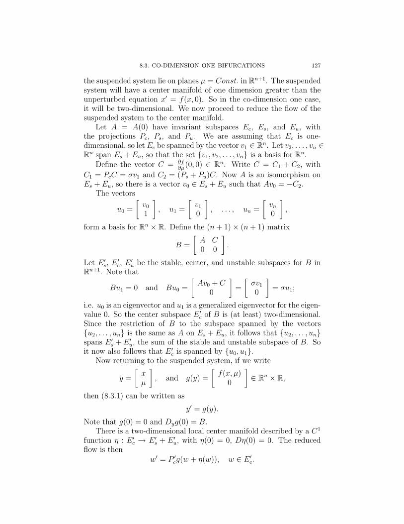
8.3. CO-DIMENSION ONE BIFURCATIONS 127
the suspended system lie on planes µ = Const. in Rn+1. The suspendedsystem will have a center manifold of one dimension greater than theunperturbed equation x′ = f(x, 0). So in the co-dimension one case,it will be two-dimensional. We now proceed to reduce the flow of thesuspended system to the center manifold.
Let A = A(0) have invariant subspaces Ec, Es, and Eu, withthe projections Pc, Ps, and Pu. We are assuming that Ec is one-dimensional, so let Ec be spanned by the vector v1 ∈ Rn. Let v2, . . . , vn ∈Rn span Es + Eu, so that the set v1, v2, . . . , vn is a basis for Rn.
Define the vector C = ∂f∂µ
(0, 0) ∈ Rn. Write C = C1 + C2, with
C1 = PcC = σv1 and C2 = (Ps + Pu)C. Now A is an isomorphism onEs + Eu, so there is a vector v0 ∈ Es + Eu such that Av0 = −C2.
The vectors
u0 =
[v0
1
], u1 =
[v1
0
], . . . , un =
[vn
0
],
form a basis for Rn × R. Define the (n+ 1)× (n+ 1) matrix
B =
[A C0 0
].
Let E ′s, E
′c, E
′u be the stable, center, and unstable subspaces for B in
Rn+1. Note that
Bu1 = 0 and Bu0 =
[Av0 + C
0
]=
[σv1
0
]= σu1;
i.e. u0 is an eigenvector and u1 is a generalized eigenvector for the eigen-value 0. So the center subspace E ′
c of B is (at least) two-dimensional.Since the restriction of B to the subspace spanned by the vectorsu2, . . . , un is the same as A on Es + Eu, it follows that u2, . . . , unspans E ′
s + E ′u, the sum of the stable and unstable subspace of B. So
it now also follows that E ′c is spanned by u0, u1.
Now returning to the suspended system, if we write
y =
[xµ
], and g(y) =
[f(x, µ)
0
]∈ Rn × R,
then (8.3.1) can be written as
y′ = g(y).
Note that g(0) = 0 and Dyg(0) = B.There is a two-dimensional local center manifold described by a C1
function η : E ′c → E ′
s + E ′u, with η(0) = 0, Dη(0) = 0. The reduced
flow is thenw′ = P ′
cg(w + η(w)), w ∈ E ′c.
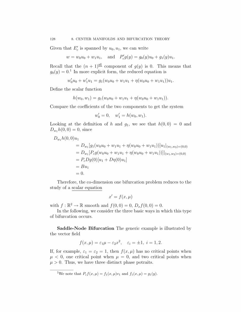
128 8. CENTER MANIFOLDS AND BIFURCATION THEORY
Given that E ′c is spanned by u0, u1, we can write
w = w0u0 + w1u1, and P ′cg(y) = g0(y)u0 + g1(y)u1.
Recall that the (n + 1)st component of g(y) is 0. This means thatg0(y) = 0.1 In more explicit form, the reduced equation is
w′0u0 + w′1u1 = g1(w0u0 + w1u1 + η(w0u0 + w1u1))u1.
Define the scalar function
h(w0, w1) = g1(w0u0 + w1u1 + η(w0u0 + w1u1)).
Compare the coefficients of the two components to get the system
w′0 = 0, w′1 = h(w0, w1).
Looking at the definition of h and g1, we see that h(0, 0) = 0 andDw1h(0, 0) = 0, since
Dw1h(0, 0)u1
= Dw1 [g1(w0u0 + w1u1 + η(w0u0 + w1u1))]u1|(w1,w2)=(0,0)
= Dw1 [Pcg(w0u0 + w1u1 + η(w0u0 + w1u1))]|(w1,w2)=(0,0)
= PcDg(0)[u1 +Dη(0)u1]
= Bu1
= 0.
Therefore, the co-dimension one bifurcation problem reduces to thestudy of a scalar equation
x′ = f(x, µ)
with f : R2 → R smooth and f(0, 0) = 0, Dxf(0, 0) = 0.In the following, we consider the three basic ways in which this type
of bifurcation occurs.
Saddle-Node Bifurcation The generic example is illustrated bythe vector field
f(x, µ) = ε1µ− ε2x2, εi = ±1, i = 1, 2.
If, for example, ε1 = ε2 = 1, then f(x, µ) has no critical points whenµ < 0, one critical point when µ = 0, and two critical points whenµ > 0. Thus, we have three distinct phase potraits.
1We note that Pcf(x, µ) = f1(x, µ)v1 and f1(x, µ) = g1(y).
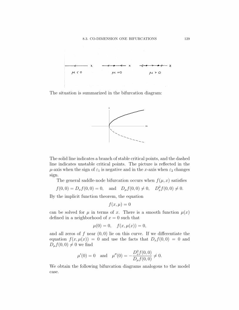
8.3. CO-DIMENSION ONE BIFURCATIONS 129
The situation is summarized in the bifurcation diagram:
mu
x
The solid line indicates a branch of stable critical points, and the dashedline indicates unstable critical points. The picture is reflected in theµ-axis when the sign of ε1 is negative and in the x-axis when ε2 changessign.
The general saddle-node bifurcation occurs when f(µ, x) satisfies
f(0, 0) = Dxf(0, 0) = 0, and Dµf(0, 0) 6= 0, D2xf(0, 0) 6= 0.
By the implicit function theorem, the equation
f(x, µ) = 0
can be solved for µ in terms of x. There is a smooth function µ(x)defined in a neighborhood of x = 0 such that
µ(0) = 0, f(x, µ(x)) = 0,
and all zeros of f near (0, 0) lie on this curve. If we differentiate theequation f(x, µ(x)) = 0 and use the facts that Dxf(0, 0) = 0 andDµf(0, 0) 6= 0 we find
µ′(0) = 0 and µ′′(0) = −D2xf(0, 0)
Dµf(0, 0)6= 0.
We obtain the following bifurcation diagrams analogous to the modelcase.
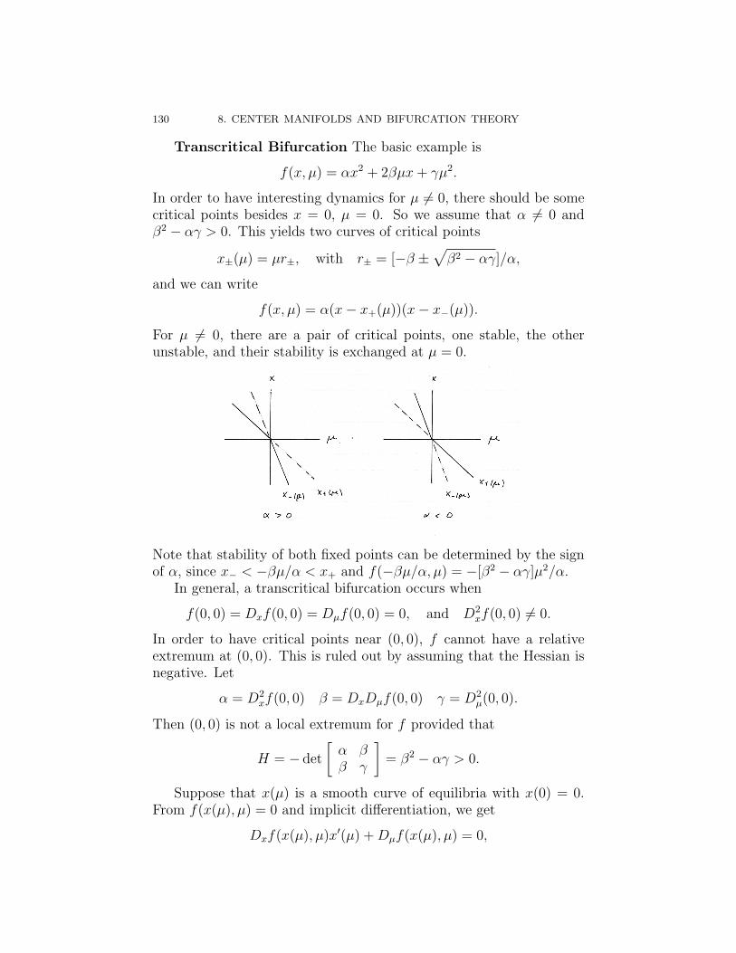
130 8. CENTER MANIFOLDS AND BIFURCATION THEORY
Transcritical Bifurcation The basic example is
f(x, µ) = αx2 + 2βµx+ γµ2.
In order to have interesting dynamics for µ 6= 0, there should be somecritical points besides x = 0, µ = 0. So we assume that α 6= 0 andβ2 − αγ > 0. This yields two curves of critical points
x±(µ) = µr±, with r± = [−β ±√β2 − αγ]/α,
and we can write
f(x, µ) = α(x− x+(µ))(x− x−(µ)).
For µ 6= 0, there are a pair of critical points, one stable, the otherunstable, and their stability is exchanged at µ = 0.
Note that stability of both fixed points can be determined by the signof α, since x− < −βµ/α < x+ and f(−βµ/α, µ) = −[β2 − αγ]µ2/α.
In general, a transcritical bifurcation occurs when
f(0, 0) = Dxf(0, 0) = Dµf(0, 0) = 0, and D2xf(0, 0) 6= 0.
In order to have critical points near (0, 0), f cannot have a relativeextremum at (0, 0). This is ruled out by assuming that the Hessian isnegative. Let
α = D2xf(0, 0) β = DxDµf(0, 0) γ = D2
µ(0, 0).
Then (0, 0) is not a local extremum for f provided that
H = − det
[α ββ γ
]= β2 − αγ > 0.
Suppose that x(µ) is a smooth curve of equilibria with x(0) = 0.From f(x(µ), µ) = 0 and implicit differentiation, we get
Dxf(x(µ), µ)x′(µ) +Dµf(x(µ), µ) = 0,
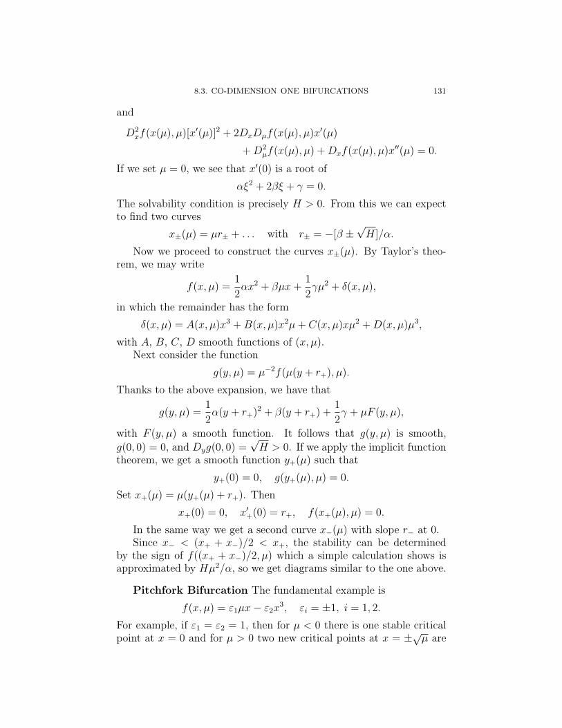
8.3. CO-DIMENSION ONE BIFURCATIONS 131
and
D2xf(x(µ), µ)[x′(µ)]2 + 2DxDµf(x(µ), µ)x′(µ)
+D2µf(x(µ), µ) +Dxf(x(µ), µ)x′′(µ) = 0.
If we set µ = 0, we see that x′(0) is a root of
αξ2 + 2βξ + γ = 0.
The solvability condition is precisely H > 0. From this we can expectto find two curves
x±(µ) = µr± + . . . with r± = −[β ±√H]/α.
Now we proceed to construct the curves x±(µ). By Taylor’s theo-rem, we may write
f(x, µ) =1
2αx2 + βµx+
1
2γµ2 + δ(x, µ),
in which the remainder has the form
δ(x, µ) = A(x, µ)x3 +B(x, µ)x2µ+ C(x, µ)xµ2 +D(x, µ)µ3,
with A, B, C, D smooth functions of (x, µ).Next consider the function
g(y, µ) = µ−2f(µ(y + r+), µ).
Thanks to the above expansion, we have that
g(y, µ) =1
2α(y + r+)2 + β(y + r+) +
1
2γ + µF (y, µ),
with F (y, µ) a smooth function. It follows that g(y, µ) is smooth,
g(0, 0) = 0, and Dyg(0, 0) =√H > 0. If we apply the implicit function
theorem, we get a smooth function y+(µ) such that
y+(0) = 0, g(y+(µ), µ) = 0.
Set x+(µ) = µ(y+(µ) + r+). Then
x+(0) = 0, x′+(0) = r+, f(x+(µ), µ) = 0.
In the same way we get a second curve x−(µ) with slope r− at 0.Since x− < (x+ + x−)/2 < x+, the stability can be determined
by the sign of f((x+ + x−)/2, µ) which a simple calculation shows isapproximated by Hµ2/α, so we get diagrams similar to the one above.
Pitchfork Bifurcation The fundamental example is
f(x, µ) = ε1µx− ε2x3, εi = ±1, i = 1, 2.
For example, if ε1 = ε2 = 1, then for µ < 0 there is one stable criticalpoint at x = 0 and for µ > 0 two new critical points at x = ±√µ are
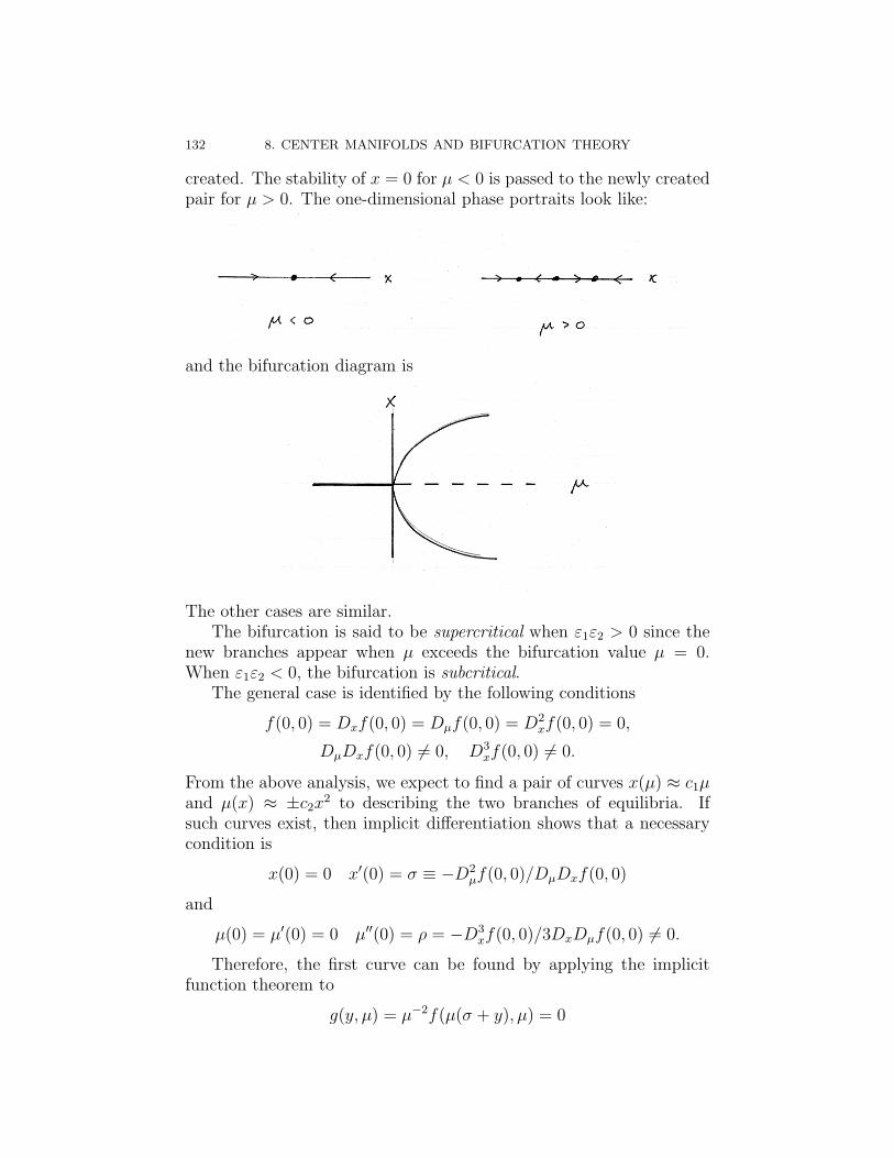
132 8. CENTER MANIFOLDS AND BIFURCATION THEORY
created. The stability of x = 0 for µ < 0 is passed to the newly createdpair for µ > 0. The one-dimensional phase portraits look like:
and the bifurcation diagram is
The other cases are similar.The bifurcation is said to be supercritical when ε1ε2 > 0 since the
new branches appear when µ exceeds the bifurcation value µ = 0.When ε1ε2 < 0, the bifurcation is subcritical.
The general case is identified by the following conditions
f(0, 0) = Dxf(0, 0) = Dµf(0, 0) = D2xf(0, 0) = 0,
DµDxf(0, 0) 6= 0, D3xf(0, 0) 6= 0.
From the above analysis, we expect to find a pair of curves x(µ) ≈ c1µand µ(x) ≈ ±c2x2 to describing the two branches of equilibria. Ifsuch curves exist, then implicit differentiation shows that a necessarycondition is
x(0) = 0 x′(0) = σ ≡ −D2µf(0, 0)/DµDxf(0, 0)
and
µ(0) = µ′(0) = 0 µ′′(0) = ρ = −D3xf(0, 0)/3DxDµf(0, 0) 6= 0.
Therefore, the first curve can be found by applying the implicitfunction theorem to
g(y, µ) = µ−2f(µ(σ + y), µ) = 0
8.3. CO-DIMENSION ONE BIFURCATIONS 133
to get y(µ) satisfying
y(0) = 0, g(y(µ), µ) = 0.
Then the curve is obtained by setting x(µ) = µ(σ + y(µ)).The second branch comes by considering the equation
h(x, λ) = x−2f(x, x2(ρ/2 + λ)) = 0.
The implicit function theorem yields a function λ(x) such that
λ(0) = 0, g(x, λ(x)) = 0.
Finally, let µ(x) = x2(ρ/2 + λ(x)). The bifurcation is supercriticalwhen ρ > 0 and subcritical when ρ < 0.
Example: The Lorentz Equation, II. Let’s have another lookat the Lorentz equations considered in section 8.2. This time, however,we add a small bifurcation parameter:
x′1 = −σx1 + σx2
x′2 = (1 + µ)x1 − x2 − x1x3
x′3 = −βx3 + x1x2.
Here β, σ > 0 are regarded as being fixed, and µ ∈ R is small. Thesystem has the form x′ = f(x, µ) with f(0, 0) = 0. Moreover, we havealready seen that the matrix
Dxf(0, 0) =
−σ σ 01 −1 00 0 −β
,has a one-dimensional center subspace, so that for µ 6= 0 a bifurcationcould occur. To study possible bifurcations near (x, µ) = (0, 0), wewill consider the suspended system and reduce to the flow on the localcenter manifold. The suspended system is:
x′1 = −σx1 + σx2
x′2 = x1 − x2 + µx1 − x1x3
x′3 = −βx3 + x1x2
µ′ = 0.
Notice that because µ is being regarded as a dependent variable, µx1
is considered to be a nonlinear term. So we are going to approximatethe flow on the two-dimensional center manifold of the equation
(8.3.2) z′ = Az + g(z),
134 8. CENTER MANIFOLDS AND BIFURCATION THEORY
where
z =
x1
x2
x3
µ
, A =
−σ σ 0 0
1 −1 0 00 0 −β 00 0 0 0
,
g(z) =
0
x1(µ− x3)x1x2
0
.(8.3.3)
By our earlier calculations, we have the following eigenvalues:
λ = 0,−(σ + 1),−β, 0and corresponding eigenvectors:
1100
,−σ
100
,
0010
,
0001
,for the matrix A. Thus, the matrix
S =
1 −σ 0 01 1 0 00 0 1 00 0 0 1
can be used to diagonalize A:
AS = SB, with B = diag(0,−(σ + 1),−β, 0).
If we make the change of coordinates z = Sy, then (8.3.2), (8.3.3)becomes
y′ = By + h(y),
in which h(y) = S−1g(Sy). More explicitly, we have
S−1 =
1
σ+1σ
σ+10 0
− 1σ+1
1σ+1
0 00 0 1 00 0 0 1
and hence
h(y) =
σ
σ+1(y1 − σy2)(y4 − y3)
1σ+1
(y1 − σy2)(y4 − y3)(y1 − σy2)(y1 + y2)
0
.Tracing back through the substitutions, we have y4 = z4 = µ.
8.3. CO-DIMENSION ONE BIFURCATIONS 135
The local center manifold is described as
W locc (0) = y ∈ R4 : Psy = η(Pcy),
with η : Ec → Es a C1 map such that η(0) = 0, Dη(0) = 0. Since Bis diagonal, it follows that Ec = spane1, e4 and E2 = spane2, e3.Given the form of Ec and Es, we can write
W locc (0) = y ∈ R4 : η1(y1, y4) = η4(y1, y4) = 0,
y2 = η2(y1, y4), y3 = η3(y1, y4).Using theorem 8.1.2, we can approximate η to third order. We findthat if H(y) satisfies
−(σ + 1)H2(y1, y4) +1
σ + 1y1y4 = O(|y|3)
−βH3(y1, y4) + y21 = O(|y|3),
then η(y) = H(y) +O(|y|3). This shows that
η2(y1, y4) = (σ + 1)−2y1y4 +O(|y|3), η3(y1, y4) = β−1y21 +O(|y|3).
By part (iii) of corollary 8.1.1, the flow on W locc (0) is governed by
w′ = Pch(w + η(w)), w = Pcy,
which, in this case, is equivalent to
y′1 =σ
σ + 1(y1 − ση2(y1, y4))(y4 − η3(y1, y4))
y′4 = 0,
with initial conditions y1(0) and y4(0) = µ. Since y4 = Const. = µ, weend up with a scalar equation for u = y1 of the form
u′ = F (u, µ),
with
F (u, µ) =σ
σ + 1(u− ση2(u, µ))(µ− η3(u, µ))
≈ σ
σ + 1
[u− σ
(σ + 1)2µu
] [µ− 1
βu2
]+ . . .
=σ
σ + 1
[µu− 1
βu3 − σ
(σ + 1)2µ2u
]+ . . .
Notice that
F (0, 0) = DuF (0, 0) = DµF (0, 0) = D2uF (0, 0) = 0,
and
DuDµF (0, 0) =σ
σ + 1> 0, D3
uF (0, 0) =6σ
β(σ + 1)> 0.
136 8. CENTER MANIFOLDS AND BIFURCATION THEORY
Thus we have a supercritical pitchfork bifurcation. For µ ≤ 0 thereis a single asymptotically stable fixed point at x = 0. If µ < 0, then allsolutions decay towards the origin exponentially fast. For µ > 0 thereis an unstable fixed point at x = 0. It has a two-dimensional stablemanifold and a one-dimensional unstable manifold. Additionally, thereare a pair of asymptotically stable fixed points. These three criticalpoints lie on the invariant curve obtained by intersecting the centermanifold of the suspended equation with the plane µ = Const. Thiscurve contains the unstable manifold of x = 0.
8.4. Poincare Normal Forms
The analysis of the reduced flow on the center manifold can be adifficult task in more than one dimension. In 1D, we have seen how theisolation of certain terms of the Taylor expansion of the vector field isessential in understanding the nature of a bifurcation. The reductionto normal form is a systematic procedure for eliminating all inessentialterms.
Consider the flow of
(8.4.1) x′ = Ax+ f(x)
where A is an n×n real matrix and f : Rn → Rn is C∞ with f(0) = 0,Df(0) = 0. Suppose we make a change of variables
(8.4.2) x = y + h(y) = Φ(y),
with h : Rn → Rn in C∞ and h(0) = 0, Dh(0) = 0. The inversefunction theorem ensures us that Φ is a local diffeomorphism near theorigin. That is, there exist neighborhoods of the origin U , V ⊂ Rn
such that Φ : U → V is a diffeomorphism.Let’s see what happens to the system under this change of coordi-
nates. Suppose that x(t) is a solution of (8.4.1) in V and define y(t)through (8.4.2). By the chain rule, we have
x′ = y′ +Dh(y)y′ = [I +Dh(y)]y′.
Then using the fact that x is a solution and then the invertibility ofDΦ, we get
y′ = [I +Dh(y)]−1x′
= [I +Dh(y)]−1[Ax+ f(x)]
= [I +Dh(y)]−1x′
= [I +Dh(y)]−1[A(y + h(y)) + f(y + h(y))].(8.4.3)
This isn’t as bad as the averaging lemma where we studied the nonau-tonomous analog of this computation!
8.4. POINCARE NORMAL FORMS 137
Suppose that the terms of the Taylor expansion of f(x) at x = 0all have degree r ≥ 2. Write
f(x) = fr(x) +O(|x|r+1),
where fr(x) is a vector field all of whose components are homogeneouspolynomials of degree r and O(|x|r+1) stands for a smooth functionwhose Taylor expansion at x = 0 starts with terms of degree at leastr + 1. Take the function h(y) in the coordinate change (8.4.2) to havethe same form as fr(x), that is, suppose that h(y) is a vector-valuedhomogeneous polynomial of degree r. Then since
[I +Dh(y)]−1 = I −Dh(y) +Dh(y)2 − . . . = I −Dh(y) +O(|y|2(r−1)),
we have when we go back to (8.4.3)
y′ = Ay + Ah(y)−Dh(y)Ay + fr(y) +O(|y|r+1).
Then expressionAh(y)−Dh(y)Ay + fr(y)
is homogeneous of degree r. We can attempt to kill these terms bychoosing the function h(y) so that
(8.4.4) LAh(y) ≡ Dh(y)Ay − Ah(y) = fr(y).
The expression LA is known as the Poisson or Lie bracket of the vectorfields Ax and h(x).
Equation (8.4.4) is really just a linear algebra problem. The setof all homogeneous vector-valued polynomials of degree r in Rn is afinite-dimensional vector space, call it Hn
r , and LAHnr → Hn
r is a linear
map. (The dimension of Hnr is n
(r + n− 1
r
).) So we are looking for
a solution of the linear system LAh = fr in Hnr .
When does (8.4.4) have solutions? In order to more easily examineour linear system in the vector space Hn
r , we need to introduce a bit ofnotation. An n-tuple of nonnegative integers
m = (m1,m2, . . . ,mn)
is called a multi-index. Its order or degree is defined to be
|m| = m1 +m2 + . . .+mn.
Given an n-tuple y = (y1, y2, . . . , yn) ∈ Rn and a multi-index m ofdegree r, monomials of degree r are conveniently notated as
ym = ym11 ym2
2 · · · ymnn .
Now if vknk=1 is a basis for Rn, then
ymvk : k = 1, . . . , n; |m| = r
138 8. CENTER MANIFOLDS AND BIFURCATION THEORY
is a basis for Hnr .
Lemma 8.4.1. Let A be an n × n matrix, and let λ = (λ1, . . . , λn)be its n-tuple of eigenvalues. Then the eigenvalues of the linear trans-formation LA on Hn
r are given by
λ ·m− λj
where |m| = r is an multi-index of degree r and j = 1, . . . , n.
Remarks on the proof. Suppose that A has a basis of eigenvec-tors v1, . . . , vn ∈ Cn with corresponding eigenvalues λ = (λ1, . . . , λn) ∈Cn. Suppose that S is the matrix whose columns are formed by theeigenvectors of A. Set x = S−1y. Then the set of homogeneous poly-nomials xmvj : j = 1, . . . , n; |m| = r forms a basis for (complex)Hn
r as well as being a set of eigenvectors for LA. A direct calculationshows that LA xmvj = (λ ·m − λj)x
mvj. This confirms the statementabout the eigenvalues, and it also shows that, in the case that A isdiagonalizable, the range of LA is spanned by xmvj for m and j suchthat λ · m − λj 6= 0. A real basis for the range of LA is obtained bytaking real and imaginary parts. If A is not diagonalizable, things geta bit more complicated.
Definition 8.4.1. A monomial ym of degree r is resonant for A iffor some k, λ ·m− λk = 0.
Thus, if A has no resonant monomials of degree r, then LA is in-vertible on Hn
r and equation (8.4.4) has a unique solution h ∈ Hnr for
every fr ∈ Hnr .
Example: Let’s compute the resonances of degree two and three forthe matrix
A =
[0 −11 0
].
The eigenvalues of A are λ = (i,−i). First, we list λ ·m for the threemulti-indices m of degree two:
(2, 0) · (i,−i) = 2i, (1, 1) · (i,−i) = 0, (0, 2) · (i,−i) = −2i.
None of these numbers is an eigenvalue for A, so there are no resonancesof order 2.
Now we do the same thing for r = 3. There are 4 monomials ofdegree 3:
(3, 0) · (i,−i) = 3i, (2, 1) · (i,−i) = i = λ1,
(1, 2) · (i,−i) = −i = λ2, (0, 3) · (i,−i) = −3i.
8.4. POINCARE NORMAL FORMS 139
We find two resonant monomials of degree 3, namely x21x2 and x1x
22.
Definition 8.4.2. The convex hull of a set Ω ⊂ Rn is the smallestconvex set which contains Ω. The convex hull is denoted by co Ω.
Lemma 8.4.2. Let A be an n× n matrix, and let σ(A) be its spec-trum, i.e. the set containing its eigenvalues. If 0 /∈ co σ(A), then Ahas at most finitely many resonances.
Proof. Since σ(A) is finite, co σ(A) is closed. Therefore, since0 /∈ co σ(A), there is a δ > 0 such that |z| ≥ δ for all z ∈ co σ(A).
Let m be a multi-index with |m| = r. Then λ ·m/r ∈ co σ(A), so|λ ·m/r| ≥ δ.
Let M > 0 bound the eigenvalues of A: |λk| ≤ M , k = 1, . . . , n. Ifr ≥ (M + 1)/δ, then |λ ·m| ≥ rδ ≥ M + 1 > λk, k = 1, . . . ,m. Thus,xm is nonresonant if |m| ≥ (M + 1)/δ.
Remark: If A is real, then since complex eigenvalues come in con-jugate pairs, 0 /∈ co σ(A) if and only if σ(A) lies on one side of theimaginary axis.
Theorem 8.4.1. Let Ax+f(x) be a smooth vector field with f(0) =0 and Df(0) = 0. Consider the Taylor expansion of f(x) near x = 0:
f(x) = f2(x) + f3(x) + · · ·+ fp(x) +Rfp+1(x),
in which fr(x) ∈ Hnr , r = 2, . . . , p and the remainder Rfp+1 is smooth
and O(|x|p+1).For each r = 1, . . . , p decompose Hn
r as Hnr = Rr(LA) + Gr(LA),
where Rr(LA) is the range of LA on Hnr and Gr(LA) is a complementary
subspace. There exists a polynomial change of coordinates, x = Φ(y),which is invertible in a neighborhood of the origin such that the equation
x′ = Ax+ f(x)
is transformed near the origin into
y′ = Ay + g2(y) + . . .+ gp(y) +Rgp+1(y),
with gr ∈ Gr and the remainder Rgp+1 smooth and O(|y|p+1) neary = 0.
Proof. We will proceed inductively, treating terms of order r =2, . . . , p in succession. First, write
f2(x) = f2(x)− g2(x) + g2(x),
with f2(x)− g2(x) ∈ R(LA) and g2(x) ∈ G2. Let h ∈ Hn2 be a solution
ofLAh2 = f2 − g2.
140 8. CENTER MANIFOLDS AND BIFURCATION THEORY
Then x = y + h2(y) transforms x′ = Ax+ f(x) into
y′ = Ay + g2(y) + f3(y) + · · ·+ fp(y) +O(|y|p+1).
If we continue in the same manner to eliminate terms of order 3, then wewill have a coordinate change of the form y = z + h3(z) with h3 ∈ Hn
3 .The point is that this change of coordinates will not affect terms oflower order. Thus, we can proceed to cancel terms of successivelyhigher order.
Example: Consider the system x′ = Ax+ f(x) with
A =
[0 10 0
],
and f(0) = 0, Df(0) = 0. Since A has the double eigenvalue 0, allmonomials are resonant! Nevertheless, LA is nonzero, so we can removesome terms. Let’s study LA on H2
2 and determine the normal form ofdegree 2.
First, for an arbitrary function H(x) =
[H1(x)H2(x)
], we have
LAH(x) = DH(x)Ax− AH(x) =
[x2∂1H1(x)−H2(x)
x2∂1H2(x)
].
Choose a basis for H22:
h1(x) = 12x2
1e1 h4(x) = 12x2
1e2h2(x) = x1x2e1 h5(x) = x1x2e2h3(x) = 1
2x2
2e1 h6(x) = 12x2
2e2
We have used the standard basis vectors here because they are gener-alized eigenvectors for A. After a little computation, we find that
LAh1 = h2 LAh2 = 2h3
LAh3 = 0 LAh4 = −h1 + h5
LAh5 = −h2 + 2h6 LAh6 = −h3
Thus, the range of LA is given by
R(LA) = span h2, h3,−h1 + h5, h6.
8.4. POINCARE NORMAL FORMS 141
Now using Taylor’s theorem, expand f(x) to second order nearx = 0:
f(x) = f2(x) +O(|x|3)
=6∑
i=1
αihi(x) +O(|x|3)
= [α2h2(x) + α3h3(x) + α5(−h1(x) + h5(x)) + α6h6(x)]
+ [(α1 + α5)h1(x) + α4h4(x)] +O(|x|3)≡ f2(x) + g2(x) +O(|x|3),
with f2 ∈ R2(LA) and g2 ∈ G2(LA). Set
H(x) = α2h1(x) +1
2α3h2(x) + α5h4(x) +
1
2α6(h1(x)− h5(x)).
ThenLAH(x) = f2(x),
and using the transformation x = y+H(y), we can achieve the normalform
y′ = Ay + g2(y) +O(|y|3).
To complete this section we state a general theorem about reductionto normal form.
Theorem 8.4.2 (Sternberg’s Theorem). Let A be an n× n matrixwith at most a finite number of resonances. Let f : Rn → Rn be C∞
with f(0) = 0, Df(0) = 0. For any positive integer k, there exists a Ck
function h : Rn → Rn with h(0) = 0, Dh(0) = 0 such that the changeof variables x = y+ h(y) transforms x′ = Ax+ f(x) in a neighborhoodof the origin into
y′ = Ay + g2(y) + · · ·+ gp(y),
where gr ∈ Hnr \ R(LA), r = 2, . . . , p, and where p is the maximum
order of any resonance.
Remarks:
(1) The difficult proof can be found in the book of Hartman, 2nded. See theorem 12.3.
(2) The result is the smooth analogue of the Hartman-Grobmantheorem 6.2.1. It says, in particular, that if A has no reso-nances, then the flow is Ck conjugate to the linear flow.
(3) The hypothesis that A has finitely many resonances impliesthat A is hyperbolic.
142 8. CENTER MANIFOLDS AND BIFURCATION THEORY
(4) In general, the size of the neighborhood in which the transfor-mation is invertible shrinks as k increases. Nothing is beingsaid here about the existence of a C∞ change of coordinates.Theorems of that sort have been established in the analyticcase.
8.5. The Hopf Bifurcation
The Hopf bifurcation is the most common type of bifurcation. Itoccurs when a pair of distinct complex conjugate eigenvalues of anequilibrium point cross the imaginary axis as the bifucation parameteris varied. At the critical bifurcation value, there are two (nonzero)eigenvalues on the imaginary axis. So this is an example of a co-dimension two bifurcation. As the bifurcation parameter crosses thecritical value, a periodic solution is created.
The general case will be reduced to the following simple planarautonomous system, with higher order perturbative terms. For now,the illustrative paradigm is
(8.5.1)d
dt
[x1
x2
]=
[µ −ωω µ
] [x1
x2
]+ (x2
1 + x22)
[a −bb a
] [x1
x2
].
Here, as usual, µ denotes the bifurcation parameter. The remainingconstants a, b, ω are fixed with a 6= 0, ω > 0. Notice that x = 0 is afixed point, for all µ ∈ R.
The corresponding linear problem
d
dt
[x1
x2
]=
[µ −ωω µ
] [x1
x2
]has eigenvalues µ ± iω. Thus, when µ < 0, the critical point x = 0 isasymptotically stable for (8.5.1), and when µ > 0, it is unstable. Whenµ = 0, the origin is a center, since the eigenvalues lie on the imaginaryaxis.
In order to find the periodic solution of (8.5.1), we change to polarcoordinates. Let
x1 = r cos θ, x2 = r sin θ.
The equations transform into
r′ = µr + ar3
θ′ = ω + br2.
The interesting feature here is that the first equation is independentof θ. In fact, we recognize the equation for r as the basic example ofa pitchfork bifurcation. If a < 0 the bifurcation is supercritical, and ifa > 0 it is subcritical.
8.5. THE HOPF BIFURCATION 143
Suppose that a < 0. Then the asymptotically stable critical pointwhich appears at r = (−µ/a)1/2 when µ > 0 corresponds to an asymp-totically orbitally stable periodic orbit for (8.5.1). If we set α = 1/
√−a
and β = b/(−a), then this periodic solution is explicitly represented by
x1(t) = α√µ cos[(ω + βµ)t]
x2(t) = α√µ sin[(ω + βµ)t],
The amplitude is α√µ and the period is 2π/(ω + βµ).
Simple as this example is, surprisingly it contains the essential in-formation necessary for understanding the general case. However, inorder to see this it will be necessary to make several natural changesof variables.
We begin with a planar autonomous equation depending on a pa-rameter
(8.5.2) x′ = f(x, µ),
with a critical point at the origin when µ = 0, i.e. f(0, 0) = 0. Thinkof this equation as the result of reducing a higher dimensional systemwith a critical point at the origin when µ = 0 to its two-dimensionalcenter manifold. If Dxf(0, 0) is invertible, then by the implicit functiontheorem there exists a smooth curve of equilibria x(µ) for µ near 0. Ifwe set g(x, µ) = f(x + x(µ), µ), then g(0, µ) = 0. Therefore, we willconsider vector fields in this form. Altogether we will assume that
A1. f : R2 × R → R2 is C∞,A2. f(0, µ) = 0,A3. Dxf(0, 0) has eigenvalues ±iω, with ω > 0, andA4. τ(µ) = tr Dxf(0, µ) satisfies τ ′(0) 6= 0.
Condition [A3] implies thatDxf(0, µ) has eigenvalues of the form ξ(µ)±iη(µ) with ξ(0) = 0 and η(0) = ω. Assumption [A4] says that ξ′(0) 6=0, since τ(µ) = 2ξ(µ). It means that as the bifurcation parameterpasses through the origin, the eigenvalues cross the imaginary axis withnonzero speed.
The first step will be to show:
Lemma 8.5.1. Let f(x, µ) be a vector field which satisfies the as-sumptions [A1]–[A4] above. For |µ| small, there is a smooth changeof coordinates (t, x, µ) 7→ (s, y, λ) which transforms solutions x(t, µ) of(8.5.2) to solutions y(s, λ) of
(8.5.3) y′ = Aλy + g(y, λ),
144 8. CENTER MANIFOLDS AND BIFURCATION THEORY
in which g(y, λ) is smooth and
Aλ =
[λ −ωω λ
], g(0, λ) = 0, Dyg(0, λ) = 0.
Proof. Let ξ(µ)±iη(µ) denote the eigenvalues of Aµ = Dxf(0, µ).Choose a basis which reduces Aµ to canonical form:
S−1µ AµSµ =
[ξ(µ) −η(µ)η(µ) ξ(µ)
].
Then the transformation x(t, µ) = Sµy(t, µ) transforms (8.5.2) intoy′ = g(y, µ) in which g(y, µ) = S−1
µ f(Sµy, µ) still satisfies [A1]–[A4]and in addition
Dyg(0, µ) =
[ξ(µ) −η(µ)η(µ) ξ(µ)
].
Next we rescale time through the change of variables t = (ω/η(µ))s.Then y((ω/η(µ))s, µ) solves
d
dsy = h(y, µ),
with
h(y, µ) = (ω/η(µ))g(y, µ).
Again h(y, µ) satisfies [A1]–[A4], and also
Dyh(0, µ) =
ωξ(µ)
η(µ)−ω
ω ωξ(µ)
η(µ)
.Finally, because of our assumptions, the function ψ(µ) = ωξ(µ)/η(µ)
has ψ′(0) 6= 0 and is therefore locally invertible. Set λ = ψ(µ). Theny(s, λ) is a solution of y′ = h(y, λ), and
Dyh(0, λ) =
[λ −ωω λ
].
This completes the proof of the lemma.
We continue from (8.5.3) with the variables renamed. We are nowgoing to apply the normal form technique to the suspended system
x′ = Aµx+ g(x, µ), µ′ = 0.
From this point of view, we should write this as
x′ = A0x+ µx+ g(x, µ), µ′ = 0,
8.5. THE HOPF BIFURCATION 145
since µx is a quadratic term. The eigenvalues for the linearized problem
x′ = A0x, µ′ = 0
are λ = (λ1, λ2, λ3) = (iω,−iω, 0).The resonances of order |m| = 2 occur when
m = (1, 1, 0), (0, 1, 1), (1, 0, 1), (0, 0, 2).
The monomial x1x2 is nonresonant for A0, so such a term can be elim-inated unless it occurs in the third equation, which it does not. Theterm µ2 is also resonant only for the third equation where it does notappear. The only resonances of order 2 are the terms µx1 in the firstequation and µx2 in the second. So by a quadratic change of variablesin x only we can transform the system to
x′ = A0x+ µx+ g(x, µ), µ′ = 0,
in which g is at least cubic in x, µ and still with g(0, µ) = 0 andDxg(0, µ) = 0.
The resonances of order |m| = 3 are given by
m = (2, 1, 0), (1, 2, 0), (1, 1, 1), (0, 1, 2), (1, 0, 2), (0, 0, 3).
The monomials x1x2µ and µ3 correspond to resonances in the thirdequation, where they do not occur. The monomials x1µ
2 and x2µ2 are
resonant for the first two equations, but they do not appear since g isat least quadratic in x1, x2. Thus, the normal form of degree three isspanned by two vectors
‖x‖2
x1
x2
0
and ‖x‖2
x2
−x1
0
.Thus, we get using a cubic change of variables
(8.5.4) x′ = A0x+ µx+ ‖x‖2Bx+ ˜g(x, µ), µ′ = 0,
with
B =
[a −bb a
]and with ˜g of fourth order in x, µ. Moreover we also still have ˜g(0, µ) =0 and Dx
˜g(0, µ) = 0, so ˜g is at least quadratic in x1, x2.Recognize that our normal form (8.5.4) is, of course, just a pertur-
bation of the model case (8.5.1). Does the periodic solution survive theperturbation?
146 8. CENTER MANIFOLDS AND BIFURCATION THEORY
We know that the sign of the constant a is important. Accordingto Guckenheimer and Holmes
16a =[∂31 g1 + ∂1∂
22 g1 + ∂2
1∂2g2 + ∂32 g2]
+1
ω[∂1∂2g1(∂
21 g1 + ∂2
2 g1)
− ∂1∂2g2(∂21 g2 + ∂2
2 g2)
− ∂21 g1∂
22 g2 + ∂2
2 g1∂21 g2],
where
g(x, µ) =
[g1(x, µ)g2(x, µ)
],
and all derivatives are evaluated at (x, µ) = (0, 0).We will look at the supercritical case when a < 0. In the subcritical
case, an analysis similar to what follows can be performed. When a = 0,there is a so-called generalized Hopf bifurcation to a periodic solution,but its properties depend on higher order terms.
Suppose that a < 0. We will show that there is a µ0 > 0 such thatfor all 0 < µ < µ0, the annulus
(8.5.5) A = x ∈ R2 : (−µ/a)1/2 − µ3/4 ≤ ‖x‖ ≤ (−µ/a)1/2 + µ3/4is positively invariant under the flow of (8.5.4). Since A contains nocritical points, it follows by the Poincare-Bendixson theorem ?? thatA contains a periodic orbit.
Let’s check the invariance. We will show that the flow of (8.5.4)goes into A. Let x(t) be a solution of (8.5.4), let α = 1/(−a)1/2, andset r(t) = ‖x(t)‖. Multiply (8.5.4) by x/r:
r′ = µr + ar3 +x
r· ˜g(x, µ).
We have that
|xr· ˜g(x, µ)| ≤ ‖˜g(x, µ)‖ ≤ C0r
2(r2 + µ2),
and so for x ∈ A we have xr· ˜g(x, µ) = O(µ2). Now consider r =
αµ1/2 + µ3/4 on the outer boundary of A. Then
r′ = µ(αµ1/2 +µ3/4) + a(αµ1/2 +µ3/4)3 +O(µ2) = −2µ7/4 +O(µ2) < 0,
for 0 < µ ≤ µ0, sufficiently small. Similarly, if r = αµ1/2 − µ3/4, then
r′ = 2µ7/4 +O(µ2) > 0,
for 0 < µ ≤ µ0. This proves invariance.Within the regionA, it is easy to show that the trace of the Jacobian
of the vector field is everywhere negative. This means that all periodic
8.6. THE LIAPUNOV-SCHMIDT METHOD 147
solutions inside A have their nontrivial Floquet multiplier inside theunit circle and are therefore orbitally stable. It follows that there canbe only one periodic solution within A, and it encircles the origin.
Define the ball
(8.5.6) B = x ∈ R2 : ‖x‖ < |µ/a|1/2 + |µ|3/4.It is immediate to check that r′ > 0 in B \ A, so that the origin isasymptotically unstable, and there are no periodic orbits in B \ A.
On the other hand, if a < 0, µ < 0, then it is straightforward toshow that r = (x2
1 + x22)
1/2 is a strict Liapunov function for (8.5.4) inthe ball B. Thus, the origin is asymptotically stable, and there are noperiodic orbits In B.
Similar arguments can be made when a > 0.The results can be summarized in the following:
Theorem 8.5.1. Suppose that a 6= 0 and that µ0 > 0 is sufficientlysmall. Let A and B be defined as in (8.5.5), (8.5.6).
Supercritical case, a < 0: If 0 < µ < µ0, then (8.5.4) has anasymptotically orbitally stable periodic orbit inside A. It is the uniqueperiodic orbit in B. The origin is asymptotically unstable. If −µ0 <µ < 0, then the origin is asymptotically stable for (8.5.4), and thereare no periodic orbits in B.
Subcritical case, a > 0: If −µ0 < µ < 0, then (8.5.4) has an asymp-totically orbitally unstable periodic orbit inside A. It is the unique pe-riodic orbit in B. The origin is asymptotically stable. If 0 < µ < µ0,then the origin is asymptotically unstable for (8.5.4), and there are noperiodic orbits in B.
There are a few questions that remain open. Does the periodicsolution depend continuously on µ? How does the period depend on µ?In the next sections, we take a new approach to study these questions.
8.6. The Liapunov-Schmidt Method
Let X, Y , and Λ be Banach spaces. Suppose that A : X → Y is abounded linear map and that N : X × Λ → Y is a C1 map such that
N(0, 0) = 0, DxN(0, 0) = 0.
We are interested in finding nontrivial solutions x ∈ X of the nonlinearequation
(8.6.1) Ax = N(x, λ).
If A is an isomorphism, that is, A : X → Y is one-to-one and onto andA−1 : Y → X is bounded, then the implicit function theorem ensures
148 8. CENTER MANIFOLDS AND BIFURCATION THEORY
the existence of a C1 function φ : U → V from a neighborhood of theorigin in U ⊂ Λ to a neighborhood of the origin in V ⊂ X such that
Aφ(λ) = N(φ(λ), λ), λ ∈ U.The Liapunov-Schmidt technique deals with the situation where A isnot an isomorphism.
Let K ⊂ X be the nullspace of A and let R ⊂ Y be the range.Assume that
(i) There exists a closed subspace M ⊂ X such that X = M +K,and
(ii) R is closed.
It follows from the closed graph theorem the the restriction of A toM isan isomorphism onto R. These assumptions are satisfied, for example,when K is finite dimensional and R has finite co-dimension. Such anoperator is called Fredholm.
Suppose that x is some solution of (8.6.1). Write x = x1 + x2 ∈M +K. Write Y = R + S, and let PR be the projection of Y onto Ralong S. Then
Ax1 = PRN(x1 + x2, λ) = F (x1, x2, λ)(8.6.2)
(I − PR)N(x1 + x2, λ) = 0.
Turn this around. By the implicit function theorem, there exists asolution x1(x2, λ) ∈ M of (8.6.2), for (x2, λ) in a neighborhood of theorigin in K × Λ. So now we want to solve
(8.6.3) (I − PR)N(x1(x2, λ) + x2, λ) = 0.
This is called the bifurcation equation. We can then attempt to solve(8.6.3) for λ in terms of x2. If this is possible, then we get a family ofsolutions of (8.6.1) in the form
x(x2) = x1(x2, λ(x2)) + x2.
A typical situation might be the case where A is Fredholm and thatthe parameter space Λ is finite dimensional. Then (8.6.3) is a system offinitely many equations in a finite number of unknowns. We can thenattempt to solve it using the standard implicit function theorem.
8.7. Hopf Bifurcation via Liapunov-Schmidt
Let’s return to the reduced problem given at the end of section 8.5after the normal form transformation. For notational convenience, wewill drop the double tilde from ˜g.
(8.7.1) x′ = A0x+ µx+ ‖x‖2Bx+ g(x, µ),
8.7. HOPF BIFURCATION VIA LIAPUNOV-SCHMIDT 149
with
(8.7.2) A0 =
[0 −ωω 0
], B =
[a −bb a
]and
(8.7.3) g(0, µ) = 0, Dxg(x, µ) = 0, g(x, µ) = O(‖x‖2(‖x‖2 + µ2)).
We are looking for a family of periodic solutions x(t, µ) with period≈ T0 = 2π/ω and amplitude ≈ µ1/2. We shall prove:
Theorem 8.7.1. There are smooth functions µ(s), λ(s), x(s), de-fined for |s| ≤ s0, such that
µ(s) ≈ −as2 + . . . , λ(s) ≈ −bs2 + . . . ,
and when µ = µ(s), x(s) is a periodic solution of (8.7.1) of period2π(1 + λ(s))/ω satisfying ‖x(s)‖ ≤ C|s|, for some constant C which isindependent of s.
We remark that this theorem allows a = 0, however in this case weknow less about the nature of periodic solutions since theorem 8.5.1is not available. When a 6= 0, theorems 8.5.1 and 8.7.1 show that theHopf bifurcation for the perturbed case is close to the unperturbedcase.
Proof. We will account for variations in the period by introducinga second parameter. Set
y(t, λ, µ) = x((1 + λ)t, µ), λ ≈ 0.
Then y is T0-periodic if and only if x is T0(1 + λ)-periodic. Now, asimple calculation gives
y′ = A0y + λA0y + (1 + λ)µy + (1 + λ)g(y, µ).
Viewed as a function of (y, λ, µ), the right-hand side is quadratic(or higher) except for the term A0y. To be able to apply the Liapunov-Schmidt technique, we will eliminate this term by introducing rotatingcoordinates (cf. sections 7.2, 7.4). Let
U(t) = eA0t =
[cosωt − sinωtsinωt cosωt
],
and sety(t) = U(t)z(t).
Another routine calculation shows that
(8.7.4) z′ = λA0z + (1 + λ)µz + (1 + λ)U(−t)g(U(t)z, µ).
We are going to construct T0-periodic solutions of this equation.
150 8. CENTER MANIFOLDS AND BIFURCATION THEORY
Here comes the set-up for Liapunov-Schmidt. Let
X = z ∈ C1(R,R2) : z(t+ T0) = z(t),with the norm
‖z‖X = max0≤t≤T0
‖z(t)‖+ max0≤t≤T0
‖z′(t)‖.
Also, let
Y = h ∈ C0(R,R2) : h(t+ T0) = h(t),with the norm
‖h‖Y = max0≤t≤T0
‖h(t)‖
If we define L = ddt
, then L : X → Y is a bounded linear map. It isclear that the null space of L is
K = z ∈ X : z(t) = v = Const.,and that the range of L is
R = h ∈ Y :
∫ T0
0
h(t)dt = 0.
So we have
X = M +K, and Y = R + S,
with
M = z ∈ X :
∫ T0
0
z(t)dt = 0,
and
S = h ∈ Y : h(t) = Const..M is a closed subspace of X and R is a closed subspace of Y , soL : M → R is an isomorphism by the closed graph theorem. (It is easyto verify this directly.) Note that L is Fredholm, since K and S arefinite (two) dimensional. The projection of Y onto R along S is givenby
PRh(t) = h(t)− 1
T0
∫ T0
0
h(s)ds.
Now our problem (8.7.4) can be encoded as
Lz = N(z, λ, µ),
in which
N(z, λ, µ) = λA0z + (1 + λ)µz
+ (1 + λ)‖z‖2U(−t)BU(t)z + (1 + λ)U(−t)g(U(t)z, µ).
8.7. HOPF BIFURCATION VIA LIAPUNOV-SCHMIDT 151
Note that N : X × R2 → Y and
(8.7.5) N(0, λ, µ) = 0, DzN(0, λ, µ) = 0.
All of the conditions for Liapunov-Schmidt are fulfilled, so we proceedto analyze the problem
Lu = PRN(u+ v, λ, µ),
(I − PR)N(u+ v, λ, µ) = 0,
with u ∈M and v ∈ K = R2.By the implicit function theorem, we get a C1 mapping φ(v, λ, µ)
from a neighborhood of the origin in R2 × R× R into M such that
φ(0, 0, 0) = 0 and Lφ(v, λ, µ) = PRN(φ(v, λ, µ) + v, λ, µ).
By the uniqueness part of the implicit function theorem, we get thatφ(0, λ, µ) = 0. Next, from
LDvφ(v, λ, µ) = PR[DzN(φ(v, λ, µ) + v, λ, µ)(Dvφ(v, λ, µ) + I)],
we see using (8.7.5) that
LDvφ(0, λ, µ) = PR[DzN(0, λ, µ)(Dvφ(0, λ, µ) + I)] = 0.
It follows that Dvφ(0, λ, µ) = 0, since L is an isomorphism.Set u(t, v, λ, µ) = φ(v, λ, µ)(t). Then
u(t, 0, λ, µ) = 0, and Dvu(t, 0, λ, µ) = 0.
We can therefore write
u(t, v, λ, µ) =
∫ 1
0
d
dσu(t, σv, λ, µ)dσ
=
∫ 1
0
Dvu(t, σv, λ, µ)vdσ
= J(t, v, λ, µ)v,
with J(t, 0, λ, µ) = 0, and J(t, v, λ, µ) smoothly dependent on v, λ, µ.
152 8. CENTER MANIFOLDS AND BIFURCATION THEORY
We now need to study the bifurcation function
B(v, λ, µ)
=(I − PR)N(φ(v, λ, µ) + v, λ, µ)
=1
T0
∫ T0
0
(I − PR)N(u(t, v, λ, µ) + v, λ, µ)dt
=[λA0 + (1 + λ)µ]v
+1 + λ
T0
∫ T0
0
‖u(t, v, λ, µ) + v‖2U(−t)BU(t)[u(t, v, λ, µ) + v]dt
+1 + λ
T0
∫ T0
0
U(−t)g(U(t)[u(t, v, λ, µ) + v], µ)dt.
Consider v in the form v = (s, 0) = se1. Define B0(s, λ, µ) =1sB(se1, λ, µ). Since u(t, se1, λ, µ) + se1 = s[J(t, se1, λ, µ) + I]e1, we
have
B0(s, λ, µ) = [λA0 + (1 + λ)µI]e1 + s2B1(s, λ, µ) + B2(s, λ, µ),
with
B1(s, λ, µ) =
1 + λ
T0
∫ T0
0
‖[J(t, v, λ, µ) + I]e1‖2U(−t)BU(t)[J(t, v, λ, µ) + I]e1dt
and
B2(s, λ, µ) =1 + λ
sT0
∫ T0
0
U(−t)g(U(t)[u(t, se1, λ, µ) + se1], µ)dt.
A straightforward calculation gives,
B1(0, 0, 0) =1 + λ
T0
∫ T0
0
U(−t)BU(t)vdt =
[ab
].
Thanks to the properties of g(x, µ), we have that
B2(0, 0, 0) =∂
∂sB2(0, 0, 0) =
∂2
∂s2B2(0, 0, 0) = 0.
Now we solve the bifurcation equation. B0 : R2 × R × R → R2 isC1, B0(0, 0, 0) = 0, and
Dλ,µB0(0, 0, 0) =
[0 1ω 0
],
is invertible. By the implicit function theorem, there are smooth curvesλ(s), µ(s) such that λ(0) = 0, µ(0) = 0, and B0(s, λ(s), µ(s)) = 0.
8.7. HOPF BIFURCATION VIA LIAPUNOV-SCHMIDT 153
This construction yields a unique (up to rotation) family of periodicsolutions
x(t, s) = U(t)[u(t/(1 + λ(s)), se1, λ(s), µ(s)) + se1].
This family depends continuously on the parameter s. The amplitudeis ≈ s, and the period is T0(1 + λ(s)).
Differentiation of the bifurcation equation with respect to s givesλ′(0) = µ′(0) = 0, and[
0 1ω 0
] [λ′′(0)µ′′(0)
]= −2
[ab
].