Embed Size (px)
Citation preview

BEN S. BERNANKE
Princeton University
MARK GERTLER
New York University
MARK WATSON
Princeton University
Systematic Monetary Policy and the Effiects of Oil Price Shocks
THE PRINCIPAL OBJECTIVE of this paper is to increase our understanding
of the role of monetary policy in postwar U. S. business cycles. We take
as our starting point two common findings in the recent monetary policy
literature based on vector autoregressions (VARs).' First, identified
shocks to monetary policy explain relatively little of the overall varia-
tion in output (typically, less than 20 percent). Second, most of the
observed movement in the instruments of monetary policy, such as the
federal funds rate or nonborrowed reserves, is endogenous; that is,
changes in Federal Reserve policy are largely explained by macroeco-
nomic conditions, as one might expect, given the Fed's commitment to
macroeconomic stabilization. These two findings obviously do not sup-
port the view that erratic and unpredictable fluctuations in Federal Re-
serve policies are a primary cause of postwar U.S. business cycles; but
neither do they rule out the possibility that systematic and predictable
monetary policies-the Fed's policy rule-affect the course of the
economy in an important way. Put more positively, if one takes the
VAR evidence on monetary policy seriously (as we do), then any case
for an important role of monetary policy in the business cycle rests on
Thanks to Benjamin Friedman, Christopher Sims, and the Brookings Panel for help-
ful comments. Expert research assistance was provided by Don Redl and Peter Simon.
The financial support of the National Science Foundation is gratefully acknowledged.
1. See, for example, Leeper, Sims, and Zha (1996).
91
This content downloaded from 128.112.71.66 on Tue, 11 Sep 2018 17:27:03 UTCAll use subject to https://about.jstor.org/terms
92 Brookings Papers on Economic Activity, 1:1997
the argument that the choice of the monetary policy rule (the "reaction
function") has significant macroeconomic effects.
Using time-series evidence to uncover the effects of monetary policy
rules on the economy is, however, a daunting task. It is not possible to
infer the effects of changes in policy rules from a standard identified
VAR system, since this approach typically provides little or no struc-
tural interpretation of the coefficients that make up the lag structure of
the model. Large-scale econometric models, such as the MIT-Penn-
SSRC model, are designed for analyzing alternative policies; but criti-
cisms of the identifying assumptions of these models have been the
subject of a number of important papers, notably, by Robert Lucas and
Christopher Sims.2 Particularly relevant to the present paper is Sims's
point that the many overidentifying restrictions of large-scale models
may be both theoretically and empirically suspect, often implying spec-
ifications that do not match the basic time-series properties of the data
particularly well. Recent progress in the development of dynamic sto-
chastic general equilibrium models overcomes much of Lucas's objec-
tion to the traditional approach, but the ability of these models to fit the
time-series data-in particular, the relationships among money, interest
rates, output, and prices-seems, if anything, worse than that of tra-
ditional large-scale models.
In this paper we take some modest (but, we hope, informative) first
steps toward sorting out the effects of systematic monetary policy on
the economy, within a framework designed to accommodate the time-
series facts about the U.S. economy in a flexible manner. Our strategy
involves adding a little bit of structure to an identified VAR. Specifi-
cally, we assume that monetary policy works its effects on the economy
through the medium of the term structure of open-market interest rates;
and that, given the term structure, the policy instrument (in our appli-
cation, the federal funds rate) has no independent effect on the econ-
omy. In combination with the expectations theory of the term structure,
this assumption allows one to summarize the effects of alternative ex-
pected future monetary policies in terms of their effects on the current
short and long interest rates, which, in turn, help to determine the
evolution of the economy. By comparing, for example, the historical
behavior of the economy with its behavior under an hypothesized alter-
2. Lucas (1976); Sims (1980).
This content downloaded from 128.112.71.66 on Tue, 11 Sep 2018 17:27:03 UTCAll use subject to https://about.jstor.org/terms
Ben S. Bernanke, Mark Gertler, and Mark Watson 93
native policy reaction function, we obtain a rough measure of the im-
portance of the systematic component of monetary policy. Our approach
is similar in spirit to a methodology due to Sims and Tao Zha; however,
these authors do not attempt to sort out the effects of anticipated and
partially unanticipated policy changes.3 While our proposed method-
ology is crude, and certainly is not invulnerable to the Lucas critique,
we believe that it represents a commonsense approach to the problem
of measuring the effects of anticipated policy, given currently available
tools.
To be able to compare historical and alternative hypothesized re-
sponses of monetary policy to economic disturbances, one needs to
select some interesting set of macroeconomic shocks to which policy is
likely to respond. We focus primarily on oil price shocks, for two
reasons.4 First, periods dominated by oil price shocks are reasonably
easy to identify empirically, and the case for exogeneity of at least the
major oil price shocks is strong (although, there is also substantial
controversy about how these shocks and their economic effects should
be modeled). Second, in the view of many economists, oil price shocks
are perhaps the leading alternative to monetary policy as the key factor
in postwar U.S. recessions: increases in oil prices preceded the reces-
sions of 1973-75, 1980-82, and 1990-91, and James Hamilton pre-
sents evidence that increases in oil prices led declines in output before
1972 as well.5 Further, one of the strongest criticisms of the neomo-
netarist claim that monetary policy has been a major cause of economic
downturns is that it may confound the effects of monetary tightening
and previous increases in oil prices.
The rest of the paper is organized as follows. We first document that
essentially all the U.S. recessions of the past thirty years have been
preceded by both oil price increases and a tightening of monetary pol-
icy, which raises the question to what extent the ensuing economic
declines can be attributed to each factor. Discussion of this identifica-
tion problem requires a digression into the parallel VAR-based literature
3. Sims and Zha (1995).
4. Hooker (1996a) also studies the effects of oil price shocks and their interaction with monetary policy in a VAR framework. However, he does not explicitly attempt to
decompose the effect of oil price shocks on the economy into a part due to the change in oil prices and a part due to the policy reaction.
5. Hamilton (1983).
This content downloaded from 128.112.71.66 on Tue, 11 Sep 2018 17:27:03 UTCAll use subject to https://about.jstor.org/terms

94 Brookings Papers on Economic Activity, 1:1997
on the effects of oil price shocks; one main conclusion is that it is
surprisingly difficult to find an indicator of oil price shocks that pro-
duces the expected responses of macroeconomic and policy variables
in a VAR setting. After comparing alternative indicators, we choose as
our principal measure of oil price shocks the "net oil price increase"
variable proposed by Hamilton.6
We next introduce our identification strategy, which summarizes the
effects of an anticipated change in monetary policy in terms of its
impact on the current term structure of interest rates (specifically, the
three-month and ten-year government rates). We show that this ap-
proach provides reasonable results for the analysis of shocks to mone-
tary policy and to oil prices; and, in particular, we find that the endog-
enous monetary policy response can account for a very substantial
portion (in some cases, nearly all) of the depressing effects of oil price
shocks on the real economy. This result is reinforced by a more dis-
aggregated analysis, which compares the effects of oil price and mon-
etary policy shocks on components of GDP. Looking more specifically
at individual recessionary episodes associated with oil price shocks, we
find that both monetary policy and other nonmoney, nonoil disturbances
played important roles, but that oil shocks, per se, were not a major
cause of these downturns. Overall, these findings help to resolve the
long-standing puzzle of the apparently disproportionate effect of oil
price increases on the economy. We also show that our method produces
reasonable results when applied to the analysis of monetary policy
reactions to other types of shocks, such as shocks to output and to
commodity prices.
After presenting the basic results, we look in more detail at their
robustness and stability. Regarding robustness, we find that the broad
conclusion that endogenous monetary policy is an important component
of the aggregate impact of oil price shocks holds across a variety of
specifications, although the exact proportion of the effect due to mon-
etary policy is sometimes hard to determine statistically. We also find
evidence of subsample instability in our estimated system. To some
extent, however, this instability helps to strengthen our main conclu-
sions about the role of endogenous monetary policy, in that the total
effect of oil price shocks on the economy on output is found to be
6. Hamilton (1996a, 1996b).
This content downloaded from 128.112.71.66 on Tue, 11 Sep 2018 17:27:03 UTCAll use subject to https://about.jstor.org/terms
Ben S. Bernanke, Mark Gertler, and Mark Watson 95
strongest during the Volcker era-when the monetary response to in-
flationary shocks was also the strongest.
Our analysis uses interpolated monthly data on GDP and its com-
ponents. Appendix A documents the construction of these data, and
appendix B describes all of the data that we use.
Is It Monetary Policy or Is It Oil? The Basic Identification
Problem
The idea that monetary policy is a major source of real fluctuations
in the economy is an old one; much of its lasting appeal reflects the
ongoing influence of the seminal work of Milton Friedman and Anna
Schwartz.7 Obtaining credible measurements of monetary policy's con-
tribution to business cycles has proved difficult, however. As discussed
above, in recent years numerous authors have addressed the measure-
ment of the effects of monetary policy by means of the VAR method-
ology, introduced into economics by Sims.8 Roughly speaking, this
approach identifies unanticipated innovations to monetary policy with
an unforecasted shock to some policy indicator, such as the federal
funds rate or the rate of growth of nonborrowed reserves. Using the
estimated VAR system, one can trace out the dynamic responses of
output, prices, and other macroeconomic variables to this innovation,
thereby obtaining quantitative estimates of how monetary policy inno-
vations affect the economy. As John Cochrane notes, "this literature
has at last produced impulse-response functions that capture common
views about monetery policy"; for example, in finding that a positive
innovation to monetary policy is followed by increases in output, prices,
and money, and by a decline in the short-term nominal interest rate.9
In addition, despite ongoing debates about precisely how the policy
innovation should be identified, the estimated responses of key mac-
roeconomic variables to a policy shock are reasonably similar across a
7. Friedman and Schwartz (1963). 8. Sims (1980); more recently, see Bernanke and Blinder (1992), Christiano and
Eichenbaum (1992), Sims (1992), Strongin (1995), Bernanke and Mihov (1995), Sims and Zha (1995), and Leeper, Sims, and Zha (1996).
9. Cochrane (1996, p. 1).
This content downloaded from 128.112.71.66 on Tue, 11 Sep 2018 17:27:03 UTCAll use subject to https://about.jstor.org/terms
96 Brookings Papers on Economic Activity, 1:1997
variety of studies and suggest that monetary policy shocks can have
significant and persistent real effects.
The VAR literature has focused on unanticipated policy shocks not
because they are quantitatively very important-indeed, the conclusion
of this literature is that policy shocks are too small to account for much
of the overall variation in output and other variables-but because it is
argued that cause and effect can be cleanly disentangled only in the
case of exogenous, or random, changes in policy. However, looking
only at unanticipated policy changes begs the question of how system-
atic, or endogenous, monetary policy changes affect the economy. '?
Earlier work on the effects of monetary policy often does not make
the distinction between anticipated and unanticipated policy changes. " I
These studies frequently find a very large role for monetary policy in
cyclical fluctuations. An important recent example of this genre is an
article by Christina Romer and David Romer. 12 Following the narrative
approach of Friedman and Schwartz, Romer and Romer use Federal
Reserve records to identify a series of dates at which, in response to
high inflation, the Fed changed policy in a sharply contractionary di-
rection. Their dates presumably correspond to policy changes with both
an unanticipated component (because they were large, or decisive) and
an anticipated component (because they were explicit responses to in-
flation); indeed, Matthew Shapiro shows that these dates are largely
forecastable. ' Romer and Romer find that their dates were typically
followed by large declines in real activity and conclude that monetary
policy plays an important role in fluctuations.
But as several critiques of Romer and Romer's article and the earlier
work on anticipated monetary policy point out, studies that blur the
10. Cochrane (1996) has emphasized that even identification of the effects of un- anticipated policy changes may hinge on distinguishing between anticipated and unan- ticipated changes, since an innovation in policy typically also changes the anticipated future path of policy. The analyst thus faces the conundrum of determining how much of the economy's response to a policy shock is due to the shock, per se, and how much is due to the change in policy anticipations engendered by the shock. The focus of this paper is different from that of Cochrane, in that we emphasize the effects of nonpolicy shocks, such as oil shocks, on anticipated monetary policy; but our methods could also be used to address the specific issue he raises.
11. Nor, for that matter, between changes in the money stock induced by policy and those induced by other factors. See, for example, Andersen and Jordan (1968).
12. Romer and Romer (1989). 13. Shapiro (1994).
This content downloaded from 128.112.71.66 on Tue, 11 Sep 2018 17:27:03 UTCAll use subject to https://about.jstor.org/terms
Ben S. Bernanke, Mark Gertler, and Mark Watson 97
distinction between anticipated and unanticipated policies suffer from
precisely the identification problem that the VAR literature has at-
tempted to avoid; namely, that it is not obvious how to distinguish the
effects of anticipated policies from the effects of the shocks to which
the policies are responding. This is not merely methodological carping,
but is potentially of great practical importance in the postwar U.S.
context, since a number of the most significant tightenings of U.S.
monetary policy have followed on the heels of major increases in the
price of imported oil. 4
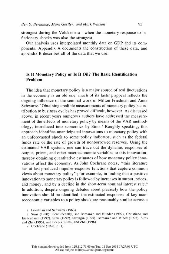
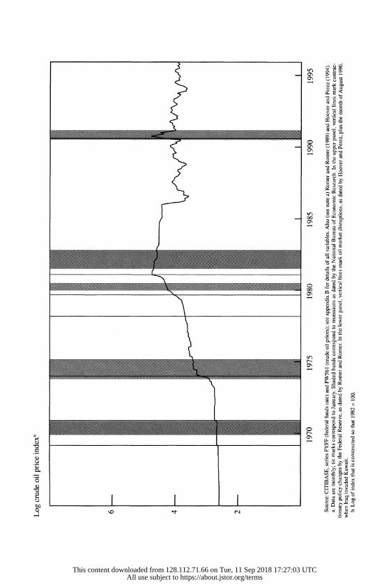
This point is illustrated in figure 1, which shows the historical be-
havior of the federal funds rate (here, taken to be an indicator of mon-
etary policy) in the upper panel and the log-level of the nominal price
of oil in the lower panel. Recessions, as dated by the National Bureau
of Economic Research, are shaded. The upper panel also indicates the
five dates identified by Romer and Romer that fall within our sample
period. The lower panel shows, in analogy to the Romer dates, seven
dates at which there were major disruptions to the oil market, as deter-
mined in part by Kevin Hoover and Stephen Perez. '5
The upper panel of figure 1, taken alone, appears to support the
neomonetarist case that tight money is the cause of recessions: each of
the first four recessions in the figure was immediately preceded by a
sharp increase in the federal funds rate, and the 1990 recession followed
a monetary tightening that ended in late 1989. Peaks in the federal
funds rate also tend to coincide with the Romer dates. However, the
lower panel of figure 1 shows why it would be premature to lay the
blame for postwar recessions at the door of the Federal Reserve: as was
first emphasized by Hamilton, nearly all of the postwar U.S. recessions
have also followed increases in the nominal price of oil, which, in turn,
have been associated with monetary tightenings. 16 Further, many of
these oil price shocks were arguably exogenous, reflecting a variety of
developments both in the Middle East and in the domestic industry, as
indicated by the Hoover-Perez dates. Thus the general identification
problem is here cast in a specific form: what portion of the last five
14. See Dotsey and Reid (1992) and Hoover and Perez (1994).
15. Hoover and Perez (1994), in their critique of the Romer and Romer approach,
introduce six dates, which are, in turn, based on a chronology due to Hamilton (1983). We have added August 1990, the month when Iraq invaded Kuwait.
16. Hamilton (1983).
This content downloaded from 128.112.71.66 on Tue, 11 Sep 2018 17:27:03 UTCAll use subject to https://about.jstor.org/terms
In
ON ON
I/N
00 ON
tC) 0
C C ON
Ct
Cu 0 Ct
Ct
I/N z
0
># C
"0 0
- 0 Cu
4) "0 4) -O
CO
4) CO
0 o o
Cl Cl - -
This content downloaded from 128.112.71.66 on Tue, 11 Sep 2018 17:27:03 UTCAll use subject to https://about.jstor.org/terms
S _ o - o' t
x~~~~~~~~O X ' 0 0
E <.o
o ON
0 -)'
CC3 C..- Ce 0u*
U 0 C
OOC
V 0- C- ,O _
___ ___ ___ ___ ___ _ ________ V .iS *
\~~~~~~~ "S O 0
.. -
CU ~~ ~~ ~~ ~~ ~~ ~~ ~~ ~~~~~~~~~~~~~~~~~~~~~~~~~~~~~~~~~~~~~~~~~~~~~~~~~~~~~~~~~~~~~~~~~~~~~~~~~~~~~1
_7 ~~~~~~~~~~~~~~~~~~~~~~~~~~13 t E
<T h8 5-o
"0 ~ ~ ~ ~ ~ ~ ~~~~~~~~~~~ 0~~~~~~~~
0 o0
C ~~~~~~~~~~~~~~~~~~~~~~~~~~~~~~~~~~~~~~~~~~~~~~~~~~~~~~~~~~~~0 &r- ?C's C'sw
This content downloaded from 128.112.71.66 on Tue, 11 Sep 2018 17:27:03 UTCAll use subject to https://about.jstor.org/terms

100 Brookings Papers on Economic Activity, 1:1 997
U.S. recessions, and of aggregate output and price fluctations in gen-
eral, was due to oil price shocks, per se, and what portion was due to
the Federal Reserve's response to those shocks? To answer this question
requires a means of measuring the effects of anticipated or systematic
monetary policies.'7
Measuring Oil Price Shocks and their Effects
We propose to identify the importance of the monetary policy feed-
back rule in a modified VAR framework. In order to do that, however,
one needs to find an appropriate indicator of oil price shocks to incor-
porate into the VAR systems. This is a more difficult task than it may
appear at first. The most natural indicator would seem to be changes in
the nominal oil price; and indeed, in an article which helped to initiate
the literature on the effects of oil price shocks, Hamilton shows that
increases in the nominal price of oil Granger-cause downturns in eco-
nomic activity.'8 However, the arrival of new data has shown this
simple measure to have a rather unstable relationship with macroeco-
nomic outcomes, leading subsequent researchers to employ increasingly
complicated specifications of the "true" relationship between oil and
the economy. II In particular, Hamilton argues in his more recent work
that the correct measure of oil shocks depends very much upon the
precise mechanism by which changes in the price of oil are supposed
to affect the economy, a question for which many answers have been
proposed but on which there is little agreement.20 For our purposes, the
exact channels through which oil affects the economy are not crucial.
17. In this paper, we take as given that anticipated as well as unanticipated monetary policies influence the real economy, owing to the existence of various nominal rigidities. Our objective is to provide an estimate of the real impact of the systematic component of monetary policy, as opposed to testing the null hypothesis that this component is neutral.
18. Hamilton (1983), to the surprise of many, also demonstrates that there appears to have been a close relationship between oil price increases and recessions even before the major OPEC shocks of the 1970s.
19. See, for example, Mork (1989), Lee, Ni, and Ratti (1995), Hamilton (1996a), and Hooker (1996a, 1996b).
20. Possibilities discussed by Hamilton (1996a) include aggregate supply effects operating through costs of production and the indirect effects of wage rigidity; aggregate demand effects; effects arising from the interaction of uncertainty about future energy prices and the irreversibility of investment; and asymmetric sectoral impacts that force costly reallocations of resources.
This content downloaded from 128.112.71.66 on Tue, 11 Sep 2018 17:27:03 UTCAll use subject to https://about.jstor.org/terms
Ben S. Bernanke, Mark Gertler, and Mark Watson 101
What matters is that one can identify an exogenous movement in the
price of oil that has a significant and a priori plausible reduced-form
impact on the economy.
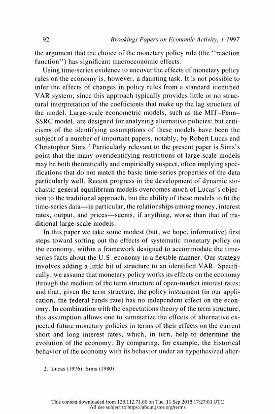
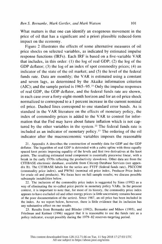
Figure 2 illustrates the effects of some alternative measures of oil
price shocks on selected variables, as indicated by estimated impulse
response functions (IRFs). Each IRF is based on a five-variable VAR
that includes, in this order: (1) the log of real GDP; (2) the log of the
GDP deflator; (3) the log of an index of spot commodity prices; (4) an
indicator of the state of the oil market; and (5) the level of the federal
funds rate. Data are monthly; the VAR is estimated using a constant
and seven lags, as determined by the Akaike information criterion
(AIC); and the sample period is 1965-95.2 Only the impulse responses
of real GDP, the GDP deflator, and the federal funds rate are shown,
in each case over a forty-eight-month horizon and for an oil price shock
normalized to correspond to a 1 percent increase in the current nominal
oil price. Dashed lines correspond to one standard error bands. As is
standard in the VAR literature on the effects of monetary policy, the
index of commodity prices is added to the VAR to control for infor-
mation that the Fed may have about future inflation which is not cap-
tured by the other variables in the system.22 The federal funds rate is
included as an indicator of monetary policy.23 The ordering of the oil
indicator after the macroeconomic variables imposes the reasonable
21 Appendix A describes the construction of monthly data for GDP and the GDP deflator. The logarithm of real GDP is detrended with a cubic spline with three equally spaced knot points imposing equality of the levels and first two derivatives at the knot points. The resulting estimated trend component is essentially piecewise linear, with a break in the early 1970s reflecting the productivity slowdown. Other data are from the
CITIBASE electronic database, available from Citicorp Database Services (see appen- dix B). The CITIBASE labels for the series are: FYFF (federal funds rate), PSCCOM (commodity price index), and PW561 (nominal oil price index, Producer Price Index for crude oil and products). We focus here on full sample results; we discuss possible subsample instabilities below.
22. The inclusion of the commodity price index is suggested by Sims (1992) as a way of eliminating the so-called price puzzle in monetary policy VARs. In the present context, it is important to note that, for most of its history, the commodity price index appears to have excluded oil and other energy prices (a little uncertainty remains because of the poor documentation of the series). Since 1987, an oil price has been included in the index. As we report below, however, there is little evidence that its inclusion has any substantive effect on our results.
23. Results from Bernanke and Blinder (1992), Bernanke and Mihov (1995), and Friedman and Kuttner (1996) suggest that it is reasonable to use the funds rate as a policy indicator, except possibly during the 1979-82 reserves-targeting period.
This content downloaded from 128.112.71.66 on Tue, 11 Sep 2018 17:27:03 UTCAll use subject to https://about.jstor.org/terms
co
_4l kr) _4l c"I kr) I II I _4 I o ~~~~~~~~~~~~~I I
Cm ~~~~I I I II I le
_ 0 I / I lOPC
_~~~~~~~~l X 6 f i = 6ci l = ~ ~ _- - , -
ii~~~~~~~~~~~~~~~~~~~~~~~~~~~~~~~~~~~~~~~~~~Z
C; C; C 99
I, Ioq" 4
O~~~~~~~
I I ~ ~ ~ ~ ~ ~ ~ ~ ~ ~ ~ ~ ~ ~~~
I I 0~~~~~~~~~~~~~~~~~~
oz loI p o dU
This content downloaded from 128.112.71.66 on Tue, 11 Sep 2018 17:27:03 UTCAll use subject to https://about.jstor.org/terms
Ben S. Bernanke, Mark Gertler, and Mark Watson 103
assumption that oil price shocks do not significantly affect the economy
within the month. Similarly, ordering the funds rate last follows the
conventional assumption that monetary policy operates with at least a
one-month lag. The results are not sensitive to these ordering assump-
tions, as we document below in the context of a larger system.
In figure 2 we report results for four alternative indicators of the
state of the oil market; one is a slight variation of the original Hamilton
indicator, the other three are more exotic indicators that have been
developed in ongoing attempts to identify a stable relationship between
oil price shocks and the economy:
-Log of the nominal Producer Price Index (PPI) for crude oil and
products; the nominal oil price, for short. Hamilton employs the log-
difference of the nominal oil price, which, given the presence of freely
estimated lag parameters, is nearly equivalent to using the log-level.
Given the other variables included in the VAR, this indicator is also
essentially the same as that used by Julio Rotemberg and Michael
Woodford.24
-Hoover-Perez. These are the oil shock dates identified by Hoover
and Perez plus August 1990, as discussed in regard to figure 1 .25 To
scale these dates by relative importance, for each month we multiply
the Hoover-Perez dummy variables by the log change in the nominal
price of oil over the three months centered on the given month.
-Mork. After the sharp oil price declines of 1985-86 failed to lead
to an economic boom, Knut Mork argued that the effects of positive
and negative oil price shocks on the economy need not be symmetric.26
Empirically, he provided evidence that only positive changes in the
relative price of oil have important effects on output. Accordingly, in
our VARs we employ an indicator that equals the log-difference of the
relative price of oil when that change is positive and otherwise is zero.2
24. Hamilton (1983); Rotemberg and Woodford (1996).
25. Hoover and Perez (1994).
26. Mork (1989).
27. We measure the relative price of oil as the PPI for crude oil divided by the GDP
deflator. Mork (1989) argues that the PPI for crude oil is a distorted measure of the
marginal cost of oil during certain periods marked by domestic price controls; he there-
fore measures oil prices by refiner acquisition cost instead, for the period for which
those data are available. We choose to stick with the crude oil PPI for simplicity, and because we feel that there are also problems with the refiner acquisition cost as a measure of the marginal cost of crude.
This content downloaded from 128.112.71.66 on Tue, 11 Sep 2018 17:27:03 UTCAll use subject to https://about.jstor.org/terms
104 Brookings Papers on Economic Activity, 1:1997
Hamilton. In response to the breakdown of the relationship be-
tween output and simpler measures of oil price shocks, Hamilton has
proposed a more complicated measure of oil price changes: the "net
oil price increase. "28 This measure distinguishes between oil price in-
creases that establish new highs relative to recent experience and in-
creases that simply reverse recent decreases. Specifically, in the context
of monthly data, Hamilton's measure equals the maximum of (a) zero
and (b) the difference between the log-level of the crude oil price for
the current month and the maximum value of the logged crude oil price
achieved in the previous twelve months. Hamilton provides some evi-
dence for the usefulness of this variable, using semiparametric methods,
and Hooker also finds it to perform well, in the sense of having a
relatively stable relationship with macroeconomic variables.29
The deficiencies of the simplest measure of the state of the oil market,
the nominal price of crude oil, are apparent from figure 2. In particular,
for our 1965-95 sample period, a shock to the nominal price of oil is
followed by a rise in output for the first year or so and by a slight short-
run decline in the price level. Both of these results (which have been
verified in the recent literature on oil price shocks) are anomalous,
relative to the conventional wisdom about the effects of oil price shocks
on the economy. As indicated in note 29, other simple measures, such
as the relative price of oil, give similarly unsatisfactory results.
The three more complex indicators (Hoover-Perez, Mork, and Ham-
ilton) produce "better looking" IRFs, in that output falls and prices
rise following an oil price shock, although generally neither response
is statistically significant. The point estimates of the effect of an oil
price shock on output suggest a modest impact from an economic per-
spective. For example, in the case of the Hamilton indicator, the sum
28. Hamilton (1996a, 1996b).
29. Hamilton (1996b); Hooker (1996a). We also experimented with VARs including the log-difference of the nominal price of oil (the indicator used by Hamilton, 1983); the log of the real price of oil (the nominal oil price divided by the GDP deflator); the log-difference of the real price of oil; and the log of the nominal price of oil weighted
by the share of energy costs in GDP (as suggested by William Nordhaus at the Brookings Panel meeting). As the results obtained were very similar to those using the log nominal price of oil, we do not report them here. The literature provides yet additional indicators of oil price shocks. Those proposed by Ferderer (1996) and Lee, Ni, and Ratti (1995), for example, focus on the volatility of oil prices rather than the level. For simplicity, we ignore these second-moment-based measures and concentrate on measures that are
functions of the level of oil prices.
This content downloaded from 128.112.71.66 on Tue, 11 Sep 2018 17:27:03 UTCAll use subject to https://about.jstor.org/terms
Ben S. Bernanke, Mark Gertler, and Mark Watson 105
of the impulse response coefficients for output over the first forty-eight
months is -0.538, implying that a 1 percent (transitory) shock to oil
prices leads to a cumulative loss of about 0.5 percent of a month's real
GDP, or 0.045 percent of a year's real GDP, over four years. As is
touched on below, more economically and statistically significant ef-
fects of oil price shocks are estimated (a) when the latter part of the
sample, which contains the somewhat anomalous 1990 episode, is omit-
ted; and (b) when the VAR system is augmented with short-term and
long-term market interest rates.
Figure 2 also shows that for all four indicators of the oil market, a
positive innovation to oil prices is followed by a rise in the funds rate
(tighter monetary policy), as expected, and the response is generally
statistically significant. This funds rate response illustrates the generic
identification problem: without further structure, it is not possible to
determine how much of the decline in output is the direct result of the
increase in oil prices, as opposed to the ensuing tightening of monetary
policy.
This brief exercise demonstrates a main result of the recent literature
on the macroeconomic effects of oil prices, that finding a measure of
oil price shocks that "works" in a VAR context is not straightforward.
It is also true that the estimated impacts of these measures on output
and prices can be quite unstable over different samples, as discussed
below. For present purposes, however, based on the evidence of the
literature and our own analysis (including figure 2), we choose the
Hamilton net oil price increase measure of oil price shocks for our basic
analyses.30 As we discuss further below, we have checked the robust-
ness of our exercises to the use of alternative oil market indicators; in
general, we find that when a given oil-market indicator yields reason-
able results in exercises like those shown in figure 2, our alternative
simulations also perform reasonably.
Measuring the Effects of Endogenous Monetary Policy
Figure 2 shows that, at least for some more complex-some might
argue, data-mined-indicators of oil prices, an exogenous increase in
the price of oil has the expected effects on the economy: output falls,
30. In particular, Hooker (1996a) finds that the Hamilton measure is the most stable
across subsamples.
This content downloaded from 128.112.71.66 on Tue, 11 Sep 2018 17:27:03 UTCAll use subject to https://about.jstor.org/terms

106 Brookin2s Pavers on Economic Activity. 1:1997
prices rise, and monetary policy tightens (presumably in response to
the inflationary pressures from the oil shock). Since James Tobin's
Brookings paper, however, it has been argued that oil and energy costs
are too small relative to total production costs to account for the entire
decline in output that, at least in some episodes, has followed increases
in the price of oil.31 A natural hypothesis, therefore, is that part of the
recessionary impact of oil price increases arises from the subsequent
monetary contraction.
Sims and Zha attempt to provide rough estimates of the contribution
of endogenous monetary policy changes in a VAR context.32 Their
approach is to "shut down" the policy response that would otherwise
be implied by the VAR estimates; for example, by setting the federal
funds rate (the monetary policy indicator) at its baseline level (the value
that it would have taken in the absence of the exogenous nonpolicy
shock). The difference between the total effect of the exogenous non-
policy shock on the system variables and the estimated effect when the
policy response is shut down is then interpreted as a measure of the
contribution of the endogenous policy response.
As Sims and Zha correctly point out, this procedure is equivalent to
combining the initial nonpolicy shock with a series of policy innova-
tions just sufficient to off-set the endogenous policy response. Implic-
itly, then, in the Sims-Zha exercise, people in the economy are repeat-
edly "surprised" by the failure of policy to respond to the nonpolicy
shock in its accustomed way. The authors argue, not unreasonably, that
it would take some time for people to learn that policy was not going
to respond in its usual way; so that, for deviations of policy from its
historical pattern that are neither too large nor too protracted, their
estimates of the policy effects may be acceptable approximations. This
justification is similar to the one that Sims uses in earlier articles for
conducting policy analyses in a VAR setting, despite the issues raised
by the Lucas critique.33
31. Tobin (1980) .See also Darby (1982), Kim and Loungani (1992), and Rotemberg
and Woodford (1996). Rotemberg and Woodford argue that a monopolistically compet-
itive market structure, which leads to changing markups over the business cycle, in
principle can explain the strong effect of oil price shocks.
32. Sims and Zha (1995). Counterfactual simulations in a VAR context have also
been performed by West (1993) and Kim (1995); neither paper distinguishes anticipated
from unanticipated movements in policy.
33. See, for example, Sims (1986).
This content downloaded from 128.112.71.66 on Tue, 11 Sep 2018 17:27:03 UTCAll use subject to https://about.jstor.org/terms

Ben S. Bernanke, Mark Gertler, and Mark Watson 107
Rather than ignoring Lucas's argument altogether, however, one
might try to accommodate it partially in the VAR context, by acknowl-
edging that it may be more important for some markets than for others.
In particular, the evidence for the relevance of the Lucas critique seems
much stronger for financial markets-for example, in the determination
of the term structure of interest rates-than in labor and product mar-
kets, which has led some economic forecasters and policy analysts to
propose and estimate models with rational expectations in the financial
market only.34 In that spirit, we modify the Sims-Zha procedure for
measuring the effects of endogenous policy by assuming that interest
rate expectations are formed rationally (and in particular, that financial
markets anticipate alternative policy paths), but that the other equations
of the VAR system are invariant to the contemplated policy change.
The latter assumption can be rationalized by assuming either that ex-
pectations of monetary policy enter the true structural equations for
output, prices, and so forth only through the term structure of interest
rates; or, if other policy-related expectations enter into those structural
equations, that (for policy changes that are not too large) these respond
more sluggishly than financial market expectations, as proposed by
Sims.35 Although our method is obviously neither fully structural nor
immune to the Lucas critique, it provides an interesting alternative to
the Sims-Zha approach.
More specifically, we consider small VAR systems that include stan-
dard macroeconomic variables, short-term and long-term interest rates,
and the federal funds rate (as an indicator of monetary policy). We
make the following assumptions:
First, that the federal funds rate does not directly affect macro-
economic variables such as output and prices; a reasonable assumption,
since the funds rate applies to a very limited set of transactions (over-
night borrowings of commercial bank reserves). Hence the funds rate
is excluded from the equations in the system determining those varia-
bles. However, the funds rate is allowed to affect macroeconomic var-
iables indirectly, through its effect on short-term and long-term interest
rates, which, in turn, are allowed to enter every equation that deter-
34. See Blanchard (1984) on the comparative relevance of the Lucas critique. See
Taylor (1993) for an example of a model with rational expectations limited to the
financial market.
35. Sims (1986).
This content downloaded from 128.112.71.66 on Tue, 11 Sep 2018 17:27:03 UTCAll use subject to https://about.jstor.org/terms
108 Brookings Papers on Economic Activity, 1. 1997
mines a macroeconomic variable. Note that the assumption that mon-
etary policy works strictly through interest rates is conservative, as it
ignores other possible channels, such as the exchange rate and the
"credit channel." In this sense, our estimates should represent a lower
bound on the contribution of endogenous monetary policy.
-Second, following many previous authors, that the macroeco-
nomic variables in the system are Wold-causally prior to all interest
rates. That is, in our monthly data, we assume that interest rates respond
to contemporaneous developments in the economy, but that changes in
interest rates do not affect "slow-moving" variables such as output and
prices within the month. This is a plausible assumption, given planning
and production lags.36
-Third, that the funds rate is Wold-causally prior to the other mar-
ket interest rates. That is, the covariation between innovations in the
funds rate and in other interest rates is caused by the influence of
monetary policy changes on interest rates, rather than by the response
of the policymakers to market rates within the month. This is a strong
assumption, although it appears to give fairly reasonable results in the
context of the expectations theory of the term structure. It may be
justified if the term premium contains no information about the econ-
omy that is not also contained in the other variables seen by the Fed.
Below, we briefly discuss an alternative ordering assumption that al-
lows for considerable reaction by the Fed to current market interest rate
movements.
Formally, let Y, denote a set of macroeconomic variables, including
the price of oil, at date t. Similarly, let R, = (Rs, RI) represent the set of market interest rates; specifically, the three-month Treasury bill rate
(the "short rate," RS) and the ten-year Treasury bond rate (the "long
rate," R,). Finally, the scalar FF, is the federal funds rate. Under the
assumptions above, the restricted VAR system is written
p
(1) Yt (I'v,Yt-i + FvriR,t-) + GN'l'Et
36. As Sims points out, however, the assumption is less plausible for the commodity
price index, which is included in the nonpolicy block as an information variable; see
Leeper, Sims, and Zha (1996).
This content downloaded from 128.112.71.66 on Tue, 11 Sep 2018 17:27:03 UTCAll use subject to https://about.jstor.org/terms
Ben S. Bernanke, Mark Gertler, and Mark Watson 109
p
(2) FF, = , a,jYt_j + nr,jR,t_ + Trr0jFF,t_)
+ Er, + G + GfE,,
(3) R, (_rr-',iYt-i + _r,.,.,jR,_j + Trl,if;ft,_)
+E>,t + Gr,! e! + G,E;,
where the rr and G terms are matrices of coefficients of the appropriate
dimensions, the E terms are vectors of orthogonal error terms, and
constant terms have been omitted for notational convenience. For equa-
tion 1, the exclusion of FFt_i follows from the first assumption above, that the funds rate does not directly affect macroeconomic variables;
and the exclusion of Er, and E11, is implied by the second assumption, that innovations to interest rates do not affect the nonpolicy variables
within the period.
In order to apply the expectations theory to identify a relationship
between the funds rate and the market interest rates, and to implement
our policy experiments, it is useful to decompose the market rates into
two parts: a part reflecting expectations of future values of the nominal
funds rate, and a term premium. We define the following variables:
tIs- I
(4) Rs = E, ( O FF,+) i 0
(5) RI= E, ( O WFF+) i 0
(6) Ss= RS-R
(7) Si RI RI
where ns = 3 months and nl = 120 months are the terms of the short-
term and long-term rates, respectively; the weights, w, are defined by ts- I ,11- I
(S.= i X P and w, = i > E 1; and E is the expectations j=O J=0
This content downloaded from 128.112.71.66 on Tue, 11 Sep 2018 17:27:03 UTCAll use subject to https://about.jstor.org/terms
110 Brookings Papers on Economic Activity, 1:1997
operator. We set the monthly discount factor, E equal to 0.997, so that
112 is equal to 0.9637. The R variables defined in equations 4 and 5 are the "expectations components" of the short and long market interest
rates, and the residual S terms in equations 6 and 7 are time-varying
term-cum-risk premiums associated with rates at the two maturities.
Note that the time series of the two components of short and long
interest rates are easily calculated from current and lagged values of Y,
FF, and R, using the estimated rr parameters in equations 1-3. In
particular, finding the estimated expectations components of short and
long rates is purely a forecasting exercise and does not require structural
identifying assumptions.
With these definitions, it is useful to rewrite the model of equations
1-3 as
p
(8) Yt [1 T7.iY,-i + 1Tvri(R,-Ji + S,_)] + GVyE t
p
(9) FF,=E (TrjY,_; + Tfr,jRt_; + 1T0jFF,t;)
+Ef, + GE,,lt + GSES, p
(10) S, = > (XA,.!jYt_ + _ srjR + XS,IFF,t;)
+ Es,t + G,VE,,t + GsfEft,
Equation 8 is identical to equation 1, except that the two market interest
rates have been broken up into their expectations and term premium
components. Equations 9 and 10 correspond to equations 2 and 3, with
the interest rates, R, replaced by the corresponding term premiums, S.
Since the difference between R and S is the expectations component of
interest rates, which is constructed as a projection on current and lagged
values of observable variables, equation 10 are equivalent to equations
2 and 3. In particular, the coefficients in equations 9 and 10 are simply
combinations of the coefficients in equation 3 and the projection coef-
ficients of the federal funds rate on current and lagged variables.
37. This weighting function and the value of I3 are suggested by Shiller, Campbell, and Schoenholz (1983).
This content downloaded from 128.112.71.66 on Tue, 11 Sep 2018 17:27:03 UTCAll use subject to https://about.jstor.org/terms

Ben S. Bernanke, Mark Gertler, and Mark Watson 111
We work with the system of equations 8-10 because it simplifies the
imposition of some alternative identifying restrictions. Our main iden-
tifying assumption, discussed above, is that the federal funds rate is
Wold-causally prior to the other interest rates in the model; this corre-
sponds to the assumption that G1, = 0 in equation 9. However, an
alternative assumption, which allows for two-way causality between
the funds rate and market rates, is that shocks to the federal funds rate
affect other interest rates contemporaneously only through their impact
on expectations of the future funds rate (that is, funds rate shocks do
not affect term premiums contemporaneously); this corresponds to the
restriction that Gs, = 0 in equation 10. Note that this alternative as- sumption allows the funds rate to respond to innovations in term pre-
miums. In both cases, we assume that GVV is lower-triangular (with ornes on the diagonal), as in conventional VAR analyses employing the Cho-
leski decomposition. In most of our applications, the "macro block"
consists of real GDP, the GDP deflator, the commodity price index,
and Hamilton's net oil price increase variable, in that order; as we
show below, our results are robust to the placement of the oil market
indicator.
To illustrate how we carry out policy experiments, consider the
scenario of greatest interest in this paper: a shock to the oil price
variable. The base case, which incorporates the effects of the endoge-
nous policy response, is calculated in the conventional way, by simu-
lating the effects of an innovation to the oil price variable using the
system of equations 8 to 10. Among the results of this exercise are the
standard impulse response functions, showing the dynamic impact of
an oil price shock on the variables of the system, including the policy
variables.
To simulate the effects of an oil price shock under a counterfactual
policy regime, we first specify an alternative path for the federal funds
rate-more specifically, deviations from the baseline impulse response
of the funds rate-in a manner analogous to the approach of Sims and
Zha.38 However, we assume that financial markets understand and an-
ticipate this alternative policy response; by assuming "maximum cred-
ibility" of the Fed's announced future policy, we stand in direct con-
trast to Sims and Zha, who assume that market participants are purely
38. Sims and Zha (1995).
This content downloaded from 128.112.71.66 on Tue, 11 Sep 2018 17:27:03 UTCAll use subject to https://about.jstor.org/terms

112 Brookings Papers on Economic Activity, 1:1997
backward-looking. To incorporate this assumption into the simulation,
we calculate the expectations component of interest rates, R,+,, i = 0, 1, ..., that is consistent with the proposed future path for the federal
funds rate. We then resimulate the effects of the oil shock in the system
of equations 8-10, imposing values of R, consistent with the assumed
path of the funds rate, and also choosing values of E11, such that the
assumed future path of the funds rate is realized. Note that this method
can be used to construct alternative impulse response functions based
on full-sample or subsample estimates and to simulate counterfactual
economic behavior for specific episodes, such as the major oil price
shocks. We use it in both ways below.
Some Policy Experiments
With the methodology described above, we are able to perform a
variety of policy experiments, using estimates from our sample period,
January 1965 through December 1995. The VAR is estimated using a
constant and seven lags, as determined by AIC.
A Monetary Policy Shock
To check on the reasonableness of the basic estimated system, we
begin with the conventional analysis of a monetary policy shock, mod-
eled here as a 25 basis point innovation to the federal funds rate. The
effects of an innovation to the federal funds rate are traced out in a
seven-variable system that includes output, the price level, the com-
modity price index, the Hamilton oil measure, the funds rate, and the
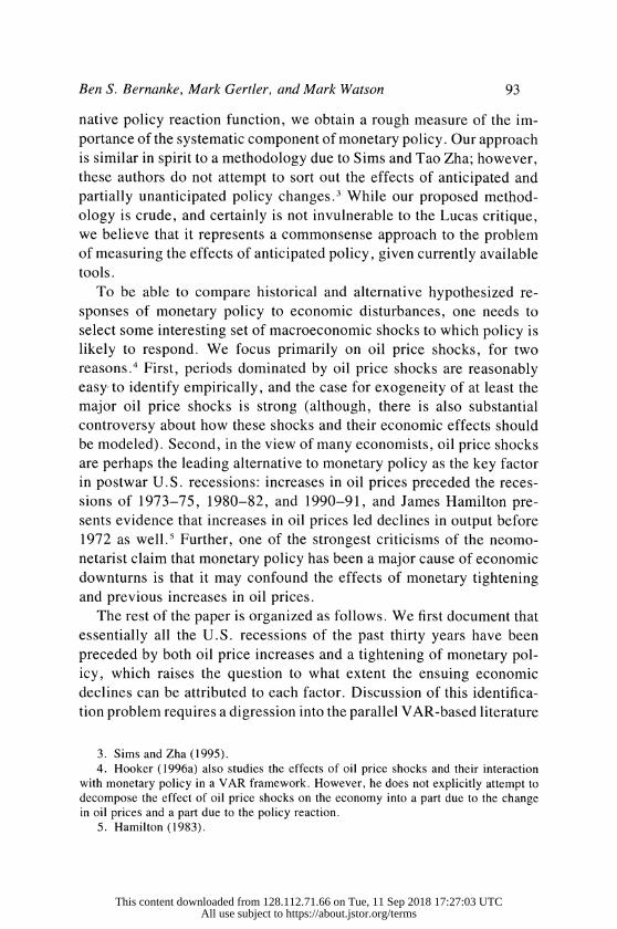
short and long term premiums. Figure 3 presents the resulting impulse
response functions. As described above, the values of the short and
long term premiums at each date are calculated by subtracting the ex-
pectations component of short and long rates (based on forecasts of
future values of the funds rate) from the short and long rates themselves.
In this base case analysis, equivalent results are obtained by directly
including the short and long rates in the VAR (ordered after the funds
rate), and the implied responses for short and long rates are included
in figure 3. In the data, there are large low-frequency movements in the
term premium of the long rate, with trend increases of about 1 per-
This content downloaded from 128.112.71.66 on Tue, 11 Sep 2018 17:27:03 UTCAll use subject to https://about.jstor.org/terms
I Cl I I
I /
I / 0
CC) / I 0,1 / C) I 'Cl- Cl
o / / 0 , - 0
I, C) , / Cl
-- II
If) 0 If) If) 0 If)
666 0 c I 0
I I I
/ r II Ii / / Ii Ii Cl // Ii II 'Cl- / / Ii / / II
C) / / 0 / / C) 0
',' - u - / / Cl Q
LL I oo II
I I / CI - I Ig 1 I II I -
-,
Cu
- - 0 'f) 0 Cu 0 0
1- 0 C- 0 1- 0 0 0 - - - - 0
'I I
00
*0 I
Cu I Cl 'Cl-
Cu o
Cu 0 0I o . - 0 C) 'C1 C,,
C) 0 'I 0o Cu 0 7 -
C)
/ Cl I /
-- /'I C)
e# Cl C- Cl
0 0 0 - 0 I/ 6oo 666
II
This content downloaded from 128.112.71.66 on Tue, 11 Sep 2018 17:27:03 UTCAll use subject to https://about.jstor.org/terms
114 Brookings Papers on Economic Activity, 1:1997
centage point in both the 1970s and the 1980s. We remove this trend
variation with a cubic spline (specified as described in note 21). As we
report in the section on robustness below, leaving the long premium
undetrended does not significantly affect the results .9 Impulse response
functions to the funds rate innovation in figure 3 are shown with one-
standard-error bands.
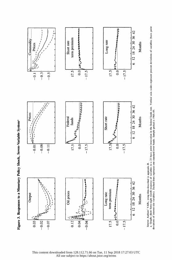
The results of this exercise will look quite familiar to those who
know the recent VAR literature on the effects of monetary policy. The
innovation to the funds rate (initially 25 basis points, peaking at about
35 basis points) is largely transitory, mostly dying away in the first nine
months. Output declines relatively quickly, reaching a trough at about
eighteen to twenty-four months and then gradually recovering. The
price level responds sluggishly, but eventually declines, nearly two
years after the policy innovation. Commodity prices also decline, and
do so much more quickly than does the general price level.
The model's only exclusion restriction, that the funds rate does not
belong in the "upper block" (which includes the oil indicator, output,
prices, and commodity prices), conditional on the presence of short-
term and long-term interest rates in that block, is marginally rejected:
the p values for the exclusion of the funds rate from the upper block
are, respectively, 0.01 for the output equation, 0.06 for the price level
equation, 0.23 for the commodity price equation, and 0.18 for the oil
equation. However, the effects of this exclusion do not seem to be
economically very significant. For example, if we compare the effects
of a funds rate shock on output in the restricted, seven-variable system
with the analogous effects in the conventional, unrestricted, five-
variable system (excluding the market interest rates), we obtain vir-
tually identical results.
An interesting new feature of the seven-variable system is that it
allows one to examine the responses of market interest rates to monetary
policy innovations, and in particular, to compare these responses to the
predictions of the pure expectations hypothesis. Looking first at short-
39. Fuhrer (1996) shows that the large movements in the long rate can be explained
in a way consistent with the expectations hypothesis if the market was making rate
forecasts at each date based on a particular set of beliefs about how the Federal Reserve's
objective function has varied over time. However, there is nothing in Fuhrer's analysis that connects these hypothesized beliefs with the actual time-series behavior of the funds
rate.
This content downloaded from 128.112.71.66 on Tue, 11 Sep 2018 17:27:03 UTCAll use subject to https://about.jstor.org/terms
Ben S. Bernanke, Mark Gertler, and Mark Watson 115
term (three-month) rates, a 25 basis point innovation to the funds rate
implies about a 15 basis point increase in the short rate, and the two
rates then decline synchronously. This seems quantitatively reasonable.
To check the consistency of this response with the expectations hypoth-
esis, one can look at the behavior of the short rate term premium, which,
by construction, is the difference between the actual short term rate and
the short term rate implied by the pure expectations hypothesis. The
short rate term premium is significantly negative immediately following
a funds rate innovation, implying that in the first month or two after an
innovation to the funds rate, the short-term interest rate is estimated to
respond less than would be predicted by the expectations hypothesis.
However, the short rate term premium quickly becomes statistically and
economically insignificant, suggesting that the expectations hypothesis
is a reasonable description of the link between the funds rate and the
short-term interest rate after the first month.
The long-term interest rate is a different story. As shown in fig-
ure 3, the long rate responds by about 5 basis points to the impact of a
25 basis point innovation in the funds rate, and the response remains
above zero for some three years, which again does not seem unreason-
able. However, comparison of the responses of the long-term interest
rate and the long rate term premium reveals that they are very close,
the latter being slightly less than the former. The implication is that the
expectations theory explains relatively little of the relationship between
the funds rate and the ten-year government bond rate. This finding is
not so surprising, given the transitory nature of funds rate shocks com-
pared with the duration of these bonds. The estimated behavior of the
long term premium thus constitutes some evidence that long rates
"overreact" to short rates, a phenomenon that has frequently been
documented in the term structure literature (although, we appear to find
less overreaction than is typically reported in the literature).40
Simulations of the Effects of an Oil Price Shock
Since our expanded model seems to perform reasonably in the case
of an innovation to monetary policy, we now turn to the exercise of
40. An alternative explanation for the overreaction of the long rate is that the policy shock is imperfectly identified. Note, for example, the slight "output puzzle"-output increases in the first few months after the policy shock. Possibly a better identification scheme would eliminate the overreaction.
This content downloaded from 128.112.71.66 on Tue, 11 Sep 2018 17:27:03 UTCAll use subject to https://about.jstor.org/terms

116 Brookings Papers on Economic Activity, 1:1997
greatest interest, which is to use the model to decompose the effects of
an oil price shock into direct and indirect (that is, through endogenous
monetary policy) components. Figure 4 shows impulse responses fol-
lowing a shock to Hamilton's net oil price increase measure under three
scenarios.
The first scenario, which we label "base," shows the impulse re-
sponses of the variables to a 1 percent innovation in the nominal price
of oil in the seven-variable system. This is a normal VAR simulation,
except that the funds rate does not enter directly into the equations for
output, prices, commodity prices, or the oil indicator. This case is
intended to show the effects on the economy of an oil price shock,
including the endogenous response of monetary policy, in contrast with
the next two simulations, which involve alternative methods of shutting
off the policy response.
The second scenario we label "Sims-Zha" (with some abuse of
terminology). In this case we simply fix the funds rate at its base values
throughout the simulation, in the manner of Sims and Zha.41 However,
recall that in contrast to the original Sims-Zha exercise, in our system
the funds rate does not enter directly into the block of macroeconomic
variables. Rather, the funds rate exerts its macroeconomic effects only
indirectly, through the short-term and long-term interest rates included
in the system. Thus in this exercise, we are effectively allowing the
change in the funds rate to act through its unconstrained, reduced-form
impact on market interest rates (which are ordered after the funds rate).
The third scenario, which we label "anticipated policy," applies our
own methodology, described above. We again set the funds rate equal
to its baseline values; that is, we shut off the response of monetary
policy to the oil shock and the changes induced by the oil shock in
output, prices, and so forth. But in this case, we let the two components
of short-term and long-term interest rates be determined separately. The
expectations component of both interest rates is set to be consistent with
the future path of the funds rate, as assumed in the scenario. The short
and long term premiums are allowed to respond as estimated in the base
model. (Below, we also consider a case where the term premiums are
kept at their baseline values.) For the simple, constant funds rate case
being examined here, the Sims-Zha and anticipated policy approaches
41. Sims and Zha (1995).
This content downloaded from 128.112.71.66 on Tue, 11 Sep 2018 17:27:03 UTCAll use subject to https://about.jstor.org/terms
Ben S. Bernanke, Mark Gertler, and Mark Watson 117
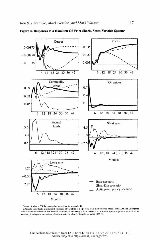
Figure 4. Responses to a Hamilton Oil Price Shock, Seven-Variable Systema
Output Prices
0.00875 0.035
- 0.00250 0.020
-0.01375 0.005
6 12 18 24 30 36 42 6 12 18 24 30 36 42
Commodity Oil prices
0.09 ~~~~~~~~0.4
0.02 i & ;' - 1 0.4
6 12 18 24 30 36 42 6 12 18 24 30 36, 42
/\ ~~~Federal Short rate
5.5 fud 4 .5l; -
3.0 .
0.5 -.
6 12 1 18 1 24 30 36 42 6 12 18 24 30 36 42
Months
1.255
-0.50 l - Base scenario - - Sims-Zha scenario
V . ._______________________ - Anticipated policy scenario 6 12 18 24 30 36 42
Months
Source: Authors' VARs, using data described in appendix B. a. Graphs show forty-eight month response of variables to a I percent Hamilton oil price shock. Sims-Zha and anticipated
policy scenarios eliminate the normal response of monetary policy. Vertical axis scales represent percent deviations of variables (basis point deviations of interest rate variables). Sample period is 1965-95.
This content downloaded from 128.112.71.66 on Tue, 11 Sep 2018 17:27:03 UTCAll use subject to https://about.jstor.org/terms
118 Brookings Papers on Economic Activity, 1:1997
show roughly similar departures from baseline. Note, however, that the
former cannot distinguish between policies that differ only in the ex-
pected future values of the funds rate, whereas, in principle, the latter
approach can make that distinction.
The results of figure 4 are reasonable, with all variables exhibiting
their expected qualitative behaviors. In particular, the absence of an
endogenously restrictive monetary policy results in higher output and
prices, as one would anticipate. Quantitatively, the effects are large, in
that a nonresponsive monetary policy suffices to eliminate most of the
output effect of an oil price shock, particularly after the first eight to
ten months. The conclusion that a substantial part of the real effects of
oil price shocks is due to the monetary policy response helps to explain
why the effects of these shocks seems larger than can easily be ex-
plained in neoclassical (flexible price) models.42
The anticipated policy simulation results in modestly higher output
and price responses than the Sims-Zha simulation in figure 4. The
differences in results occur largely because the anticipated policy sim-
ulation involves a negative short-run response in both the short and long
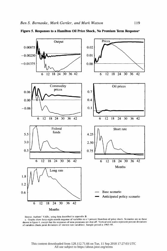
term premiums, and thus lower interest rates in the short run. Figure 5
repeats the anticipated policy simulation of figure 4, but with the re-
sponse of the term premiums shut off; that is, the funds rate is allowed
to affect the macroeconomic variables only through its effects on the
expectations component of market rates. This alternative simulation
attributes somewhat less of the recession that follows an oil shock to
the monetary policy response, but endogenous monetary policy still
accounts for two-thirds to three-fourths of the total effect of the oil
price shock on output.
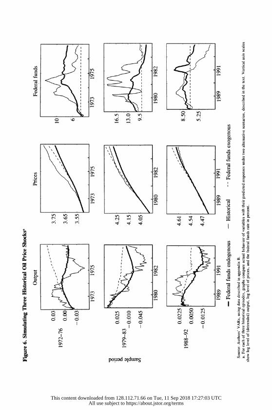
As another exercise in counterfactual policy simulation, we exam-
ine the three major oil price shocks followed by recessions: OPEC 1,
OPEC 2, and the Iraqi invasion of Kuwait. Figure 6 shows the results,
focusing on the behavior of three key variables (output, the price level,
and the funds rate) for the five-year periods surrounding each of these
episodes (respectively, 1972-76, 1979-83, and 1988-92). Each panel
shows three paths of the given variable. One line depicts the actual
historical path of the variable. The line marked "federal funds endog-
42. It should be emphasized that we are not arguing that the policies actually fol-
lowed by the Fed in the face of oil shocks were necessarily suboptimal; the usual output-
inflation trade-off is present in our simulations, and we do not attempt a welfare analysis.
This content downloaded from 128.112.71.66 on Tue, 11 Sep 2018 17:27:03 UTCAll use subject to https://about.jstor.org/terms
Ben S. Bernanke, Mark Gertler, and Mark Watson 119
Figure 5. Responses to a Hamilton Oil Price Shock, No Premium Term Responsea
Output Prices
0.00875 0.02
-0.00250 0.01
-0.01375 0.00
6 12 18 24 30 36 42 6 12 18 24 30 36 42
Commodity Oil prices
0.06 0.7
0.00 0.4
-0.06 0 X < ~ 1 0.1
6 12 18 24 30 36 42 6 12 18 24 30 36 42
Federal Short rate
5.5 4.25
3.0 2.50
0.5 0.75
6 12 18 24 30 36 42 6 12 18 24 30 36 42
Months
1.8
1.2
0.6 - Base scenario - Anticipated policy scenario
6 12 18 24 30 36 42
Months
Source: Authors' VARs, using data described in appendix B. a. Graphs show forty-eight-month response of variables to a I percent Hamilton oil price shock. Scenarios are as those
shown in figure 4, except that the responses of term premiums are shut off. Vertical axis scales represent percent deviations of variables (basis point deviations of interest rate variables). Sample period is 1965-95.
This content downloaded from 128.112.71.66 on Tue, 11 Sep 2018 17:27:03 UTCAll use subject to https://about.jstor.org/terms
I I> i 00~~~~~~~~~~~~~0
It 0~~~~
00~~~~~~~
Y~~~~~~~~0 '~ "0 00 00
o ,a
O 0ol _ sX, N <, col cO 00 ~ ~ ~ ~~~~~"
r I o o o o o o ,
*E M I I 00
00 I00
0 0 0 0~~~~~~~~~~~~~~~~~~
00~~~~~~~0 00>
pouad aldwuIS
This content downloaded from 128.112.71.66 on Tue, 11 Sep 2018 17:27:03 UTCAll use subject to https://about.jstor.org/terms

Ben S. Bernanke, Mark Gertler, and Mark Watson 121
enous" shows the behavior of the system when the oil variable is
repeatedly shocked, so that it traces out its actual historical path; all
other shocks in the system are set to zero; and the funds rate is allowed
to respond endogenously to changes in the oil variable and the induced
changes in output, prices, and other variables. This scenario is intended
to isolate the portion of each recession that results solely from the oil
price shocks and the associated monetary policy response. Finally, the
line marked "federal funds exogenous" describes the results of an
exercise in which oil prices equal their historical values, all other shocks
are shut off, and the nominal funds rate is arbitrarily fixed at a value
close to its initial value in the period. (Term premiums are allowed to
respond to the oil price shock.) This last scenario eliminates the policy
component of the effect of the oil price shock, leaving only the direct
effect of the change in oil prices on the economy.
Several observations can be made from figure 6. First, the 1974-75
decline in output is generally not well explained by the oil price shock.
The pattern of shocks reveals, instead, that the major culprit was (non-
oil) commodity prices. Commodity prices (not shown) rose very sharply
before this recession and stimulated a sharp monetary policy response
of their own, as can be seen by comparing the historical path of the
funds rate with its path in the federal funds endogenous scenario, in
which the commodity price shocks are set to zero. The federal funds
exogenous scenario, in which the funds rate responds to neither com-
modity price nor oil price shocks, exhibits no recession at all, suggest-
ing that endogenous monetary policy (responding to both oil price and
commodity price shocks) did, indeed, play an important role in this
episode.
The results for 1979-83 generally conform to the conventional wis-
dom. The decline in output through 1981 is well explained by the 1979
oil price shock and the subsequent response of monetary policy. After
the beginning of 1982, the main source of output declines (according
to this analysis) was the lagged effect of the autonomous tightening of
monetary policy in late 1980 and 1981. Note that if one excludes both
the monetary policy reaction to the oil price shocks and the autonomous
tightening of monetary policy by Federal Reserve Chairman Paul
Volcker (as in the federal funds exogenous scenario), the 1979-83
period exhibits only a modest slowdown, not a serious recession.
The experiment for 1988-92 similarly shows that shutting off the
This content downloaded from 128.112.71.66 on Tue, 11 Sep 2018 17:27:03 UTCAll use subject to https://about.jstor.org/terms

122 Brookings Papers on Economic Activity, 1:1997
policy response to oil price shocks produces a higher path of output and
prices than otherwise; again, compare the paths of the endogenous
monetary policy and exogenous monetary policy scenarios. One puzzle
that emerges is why the substantial easing of actual policy from late
1990 did not move the actual path of output closer to the alternative
policy scenario. It is possible that special factors, such as credit prob-
lems, may have been at work.
Oil, Money, and the Components of GDP
The application of our method for separating the direct effects of oil
price shocks and the indirect effects operating through the monetary
policy response leads to a rather strong conclusion: the majority of the
impact of an oil price shock on the real economy is attributable to the
central bank's response to the inflationary pressures engendered by the
shock.
A check on the plausibility of this result, using a different identifying
assumption and more disaggregated data, is provided by figure 7. This
figure is based on the seven-variable VAR system employed above (real
GDP, the GDP deflator, commodity prices, the Hamilton oil market
indicator, the funds rate, and short-term and long-term interest rates),
with the funds rate excluded from the first four equations. To this system
we add, one at a time and without feedback into the main system, eight
components of GDP: consumption, producer durables expenditure,
structures investment, inventory investment, residential investment,
government purchases, exports, and imports.43 With these systems we
conduct two experiments. First, we examine the impulse responses
obtained when the Hamilton oil price variable is shocked by 1 percent
and the federal funds rate is allowed to respond endogenously (these
responses are shown by dashed lines in figure 7). Second, we examine
the impulse responses to an exogenous federal funds rate shock of equal
maximum value to the endogenous response of the funds rate in the
first scenario (shown by solid lines). We think of this exercise as a
comparison of the total effect of an oil price shock, including the
43. Except for consumption, which is available at the monthly frequency, monthly
data for the GDP components are interpolated by state space methods; see appendix A.
Components are measured relative to the exponential of the trend for the logarithm of real GDP, as calculated from the spline regression described in note 21.
This content downloaded from 128.112.71.66 on Tue, 11 Sep 2018 17:27:03 UTCAll use subject to https://about.jstor.org/terms
1~~~ i .. - LD
02 00
*w ? ? ? O O O O c O
C) ' \ C
X ~ ~ ~ ~ N Ct 0 -L 'c E?f
0 ((B)(f 0 ()
CL 4
* CD CD O ?O O O
C, I I I I ~ I C
6 C's >-N) Q 0j -- ( 4(N)~~~~~~~~~~~~~~~~~~~~~~~~~~~~~~~~~~~~~~~~~~~~~~l
~~~~~~Cu -~~~~~~~~~~~~~~~~~~~~~~~~~ - U -~~~~~~~~~~~~~~~~~~~~~~~~~~~l
0 0 0 ~~~~~~~~~~~~~~~~~~~~~~~~~~~~~~~~~~~~~~~~~~~~~~~~~~~~~~0C
I-~~~~~~~~~~~~~~~~~~~~~~~~~~~~~~~~~~~~~~~~~~~~~~~~~~~~~~~~~~~~~~I Cu~~~~~~~~~~~~~~~~~~~~~~~~~~~~~~~
Cu~~~~~~~~~~~~~~~~~~~~~~~~~~~~~~~~~~~~~~~~~~~~~~~~~~~~~~~~~~~~~~~~~~~~~~~~~~~~~~~~~~~~~~~~~~~~~~~~'
Cu / - ~~~~~~~~~~~~~~~~~~~~~~~~~~-1 .~ ~ ~ ~~~~~~~~~~~ '
C.)~~~~~~~~~~~~~~~~~~~~~~~~~~~~~~~~~~~~~~~~~~~~~~~~~~~~~~~~~~~~~~~~~~~~~~~~~~~~~~~~~~~~~~~~~~~~~~'
-~~~~~ -I--.- (N) C) - I~~~~~~~~~~~~~~~~~~~~~~~~~~~~l
_ _ _ _ _ _ - I~~~~~~~~~~~~~~
This content downloaded from 128.112.71.66 on Tue, 11 Sep 2018 17:27:03 UTCAll use subject to https://about.jstor.org/terms
124 Brookings Papers on Economic Activity, 1:1 997
endogenous monetary response, with the effect of a monetary tightening
of similar magnitude but not associated with an oil price shock. To the
extent that the two responses are quantitatively similar, it seems rea-
sonable to attribute most of the total effect of the oil price shock to the
monetary policy response. Note, however, that we are using a different
identification assumption here than above; that is, we implicitly assume
that the economy responds in the same way to endogenous and exoge-
nous tighenings of monetary policy.
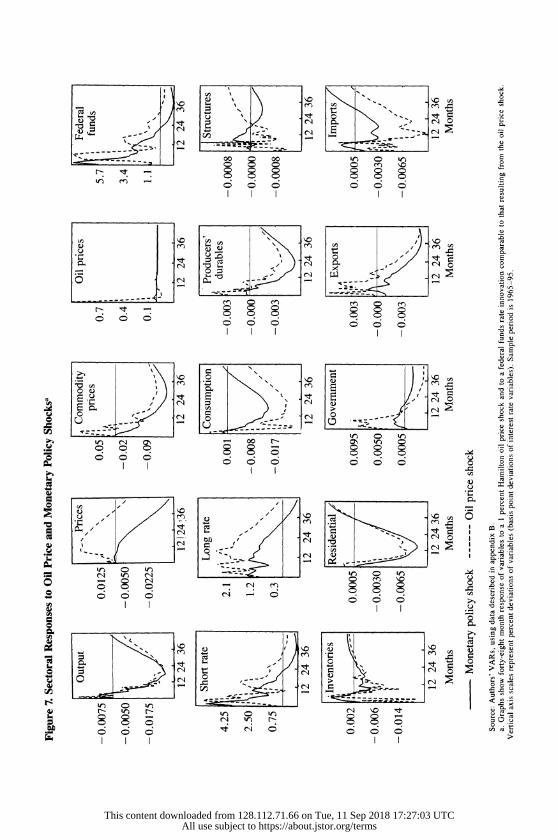
The results of shown in figure 7 provide substantial support for the
view that the monetary policy response is the dominant source of the
real effects of an oil price shock. In particular, the response of output
is virtually identical in the two scenarios, implying that it matters little
for real economic outcomes whether a change in monetary policy of a
given magnitude is preceded by an oil price shock or not. Very similar
responses across the two experiments are also found at the disaggre-
gated level, especially in equipment investment (producers' durable
equipment), inventory investment, and residential investment. Slightly
greater effects for the scenario including the oil price shock are found
for consumption and structures (although the latter difference is quan-
titatively small and statistically insignificant). Government purchases
responds more strongly in the scenario that includes the oil price shock,
for reasons that are not obvious.
The differences between the two scenarios are also instructive. The
experiment that includes the initial oil price shock does show a sub-
stantial inflationary impact in the short run, which gives some indication
as to why the Fed responds so vigorously to such shocks. On the margin,
the oil price shock also raises commodity prices and the long-term
interest rate (presumably, reflecting an increased risk premium) and it
leads to increased real exports and decreased real imports (net of terms-
of-trade effects). These responses are as expected.
Some Alternative Experiments
Although we have focused on the role of systematic monetary policy
in propagating oil price shocks, our methodology applies equally well
to other sorts of driving shocks. As a further check on the plausibility
This content downloaded from 128.112.71.66 on Tue, 11 Sep 2018 17:27:03 UTCAll use subject to https://about.jstor.org/terms
Ben S. Bernanke, Mark Gertler, and Mark Watson 125
of our method, we briefly consider two alternative cases: a shock to
commodity prices and a shock to output.
A COMMODITY PRICE SHOCK. Figure 8 looks at the effects of a shock
to the commodity price index in our original seven-variable system. As
with the oil price shock studied in figures 4 and 5, we consider three
scenarios. First, in the base scenario we calculate the impulse responses
resulting from a 1 percent innovation in commodity prices, allowing
monetary policy (as represented by the federal funds rate) to respond
in its normal way. Second, we examine the effects of shutting off the
policy response, using the Sims-Zha methodology described above.
Finally, we shut off the monetary policy response by means of our
anticipated policy approach. For simplicity, in the anticipated policy
simulation we set the responses of the term premiums to zero (as in
figure 5), so that both short-term and long-term nominal interest rates
are effectively assumed not to respond to the shock to commodity
prices.
Figure 8 shows that a 1 percent innovation in commodity prices has
an ambiguous effect on output: real GDP rises for the first year but
declines thereafter. Prices rise unambiguously. One explanation for
these results is that what we are labeling a positive shock to commodity
prices is, in fact, a mixture of an adverse shock to aggregate supply
and an expansionary shock to aggregate demand. The federal funds rate
rises sharply in response to an increase in commodity prices, which we
interpret as the Fed's response to the inflationary surge; other interest
rates also rise. The oil price indicator responds very little in the short
run to a commodity price innovation, which is reassuring, in the sense
that it confirms that the commodity and oil price variables are not
excessively collinear.
Shutting down the monetary policy response to the commodity price
shock, by either the Sims-Zha or the anticipated policy method, leads
to the expected response. Analogous to the case of oil price shocks, the
recessionary impact of a commodity price shock is eliminated and the
inflationary impact is magnified. Although it may well be the case that
the innovation in commodity prices is not a cleanly identified supply
shock, there is no evidence that an increase in commodity prices de-
presses real activity in the absence of a monetary policy response.
AN OUTPUT SHOCK. Figure 9 shows analogous results when the driving
shock is a shock to output. As with the commodity shock, we compute
This content downloaded from 128.112.71.66 on Tue, 11 Sep 2018 17:27:03 UTCAll use subject to https://about.jstor.org/terms
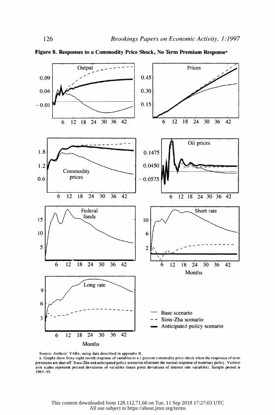
126 Brookings Papers on Economic Activity, 1:1997
Figure 8. Responses to a Commodity Price Shock, No Term Premium Response"
Output -Prices
0.09 0.455/
-0.01 0.15
6 12 18 24 30 36 42 6 12 18 24 30 36 42
- - - - - - - - - - - ~Oil prices 1.8 0.1475
1.2 0.0450
Commodity lli t. 0.6 prices - 0.0575
6 12 18 24 30 36 42 6 12 18 24 30 36 42
15 10
10 6
6 12 18 24 30 36 42 6 12 18 24 30 36 42
Months
6
- Base scenario 3 _ - - Sims-Zha scenario
- Anticipated policy scenario
6 12 18 24 30 36 42
Months
Source: Authors' VARs, using data described in appendix B. a. Graphs show forty-eight month response of variables to a I percent commodity price shock when the responses of term
premiums are shut off. Sims-Zha and anticipated policy scenarios eliminate the normal response of monetary policy. Vertical axis scales represent percent deviations of variables (basis point deviations of interest rate variables). Sample period is 1965-95.
This content downloaded from 128.112.71.66 on Tue, 11 Sep 2018 17:27:03 UTCAll use subject to https://about.jstor.org/terms

Ben S. Bernanke, Mark Gertler, and Mark Watson 127
Figure 9. Responses to an Output Shock, No Term Premium Responsea
i Output Prices
0.65 ~~~~~~~~~~1.0
0.3006
-0.05, ~~~~~~~~0.2
6 12 18 24 30 36 42 6 12 18 24 30 36 42
Commodity O . p _ - 35 5 prce 0.125pie
2.0 0.050
0.5 -0.225
6 12 18 24 30 36 42 6 12 18 24 30 36 42
52.5 | / X~~~~ederal Short rate l 52.5 fns37.5
35.0 .
17.5 1.
6 12 18 24 30 36 42 6 12 18 24 30 36 42
Months
21 , Long rate
14 '/
t Base scenario 7 F X - - Sims-Zha scenario
- ~ ~ - _ Anticipated policy scenario
6 12 18 24 30 36. 42
Months
Source: Authors' VARs, using data described in appendix B. a. Graphs show forty-eight month response of variables to a I percent output shock when the responses of term premiums
are shut off. Sims-Zha and anticipated policy scenarios eliminate the normal response of monetary policy. Vertical axis scales represent percent deviations of variables (basis point deviations of interest rate variables). Sample period is 1965- 95.
This content downloaded from 128.112.71.66 on Tue, 11 Sep 2018 17:27:03 UTCAll use subject to https://about.jstor.org/terms
128 Brookings Papers on Economic Activity, 1:1 997
the impulse response functions for three cases: a base case in which
monetary policy is allowed to respond in its normal way to the output
shock, and cases corresponding to the Sims-Zha and anitcipated policy
methods for shutting down the policy response. As before, we assume
no response of the term premiums.
Admittedly, like a shock to commodity prices, an output shock does
not have a clear a priori economic interpretation; it is an amalgam of
various random factors affecting output, holding constant the other
variables included in the system. However, based on figure 9 it seems
reasonable to interpret output shocks in this system as being dominated
by aggregate demand fluctuations: a positive output shock is followed
by increases in oil prices, commodity prices, and the general price level,
as well as in all three interest rates. Because the historical tendency of
monetary policy is to "lean against the wind," when the normal policy
response is shut off, the effects of the aggregate demand shock (as we
interpret the output shock) are all the greater. Figure 9 shows that in
the Sims-Zha and anticipated policy scenarios, the output effect of the
shock is much more persistent and prices rise by more than in the base
case. Interest rates are lower, reflecting easier monetary policy. Note
that in this analysis, the Sims-Zha and anticipated policy approaches give almost identical results.
These experiments demonstrate that our methods for shutting down
the response of monetary policy are applicable to, and give reasonable
results for, shocks other than oil price shocks. It would be interesting
to combine our methodology with identified VAR techniques that could
give a sharper structural interpretation to innovations estimated in the
macro block of the model.
Robustness and Stability
We return to our main theme, the role of systematic monetary policy
in amplifying the real effects of oil price shocks, to consider the ro-
bustness and stability of our results.
Robustness of the Results
We perform a variety of checks for robustness, some of which (such
as shutting down the term premium response) are alluded to above. To
This content downloaded from 128.112.71.66 on Tue, 11 Sep 2018 17:27:03 UTCAll use subject to https://about.jstor.org/terms

Ben S. Bernanke, Mark Gertler, and Mark Watson 129
provide more systematic information, table 1 reports some summary
statistics from alternative specifications of our VAR system. We con-
sider (a) three alternative oil-market indicators; (b) three alternative
orderings of variables within the VAR; and (c) two alternative detrend-
ing assumptions. We also calculated results for alternative measures of
output (for example, industrial production), alternative measures of the
price level (for example, the personal consumption expenditure deflator
and the consumer price index), and alternative interest rate maturities;
but since none of these variable substitutions have important effects on
our findings, they are omitted from the table.
The first row of table 1 reports results for the Hamilton oil indicator
(our base specification), whereas the second and third rows substitute
the Mork and Hoover-Perez indicators, respectively (see figure 2). The
fourth row corresponds to ordering the federal funds rate after, rather
than before, the two open market interest rates. The fifth row orders
the Hamilton oil market indicator first in the system, and the sixth row
orders the oil market indicator third-after output and prices, but before
the commodity price index. The seventh row is for a specification in
which output and the long rate term premium are not detrended, and
the eighth row reports results when all variables in the system are
detrended by a cubic spline (as described in note 21).
For each of the eight alternative specifications, table 1 reports the
effects on output and prices of a 1 percent oil price shock, under (a) a
standard simulation, allowing for the endogenous response of policy to
the oil price shock; (b) the Sims-Zha simulation, in which the federal
funds rate is fixed at its baseline value; and (c) the anticipated policy
simulation. Under the heading "output," we report the sum of the
impulse response coefficients for output for the first twenty-four months
after the oil price shock, which we employ as a measure of the output
loss associated with the shock. Under the heading "prices," we report
the twenty-fourth impulse response coefficient for prices, divided by
two, which can be interpreted as the increment in the annual average
inflation rate over the first two years following the shock. Standard
errors, calculated by Monte Carlo methods employing 500 draws per
specification, are shown in parentheses. The table also shows the dif-
ferences between the baseline (endogenous policy) specification and the
results obtained under the Sims-Zha and anticipated policy assump-
tions, again with the associated standard errors.
This content downloaded from 128.112.71.66 on Tue, 11 Sep 2018 17:27:03 UTCAll use subject to https://about.jstor.org/terms
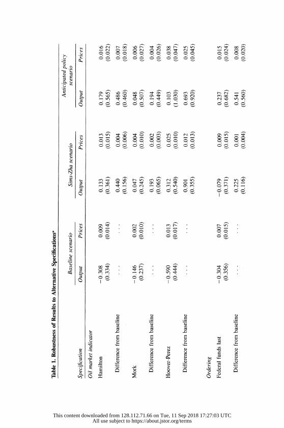
-r t-o e- i-O o- nn n- oc
Q' o- 6 6 6 66 6 66 6
W QNflo o ocr o J~ Co ~ o r-r o
t 6666666 666
X~~~~~ r-.
- ONm -Pm - ct - O r--L - D
o j- - r --
X - - Q N t - - X ~ ~ ~ ~~r - Lfo -
. 66 66 66 .. ,o- I'- o oI
0
N~~~~~~~~~ o 0 0 m 0
. -S cc 1 1 2 x 0e A P_ oN -
S o o o o o o o o0 I O - _ _ _
Cq o t N O ' > ' >0
X o - . o - . - - . o
This content downloaded from 128.112.71.66 on Tue, 11 Sep 2018 17:27:03 UTCAll use subject to https://about.jstor.org/terms
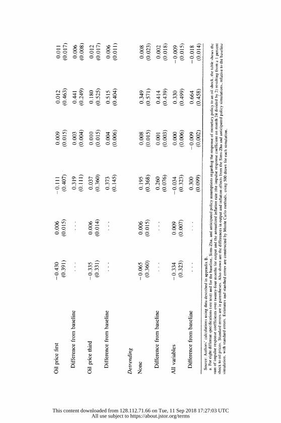
_ _ _ _ _ _ _ _ :) ( - e) --c 00 rq 1- xD o m 00 oo tr ct C)- o - - (= (= - -- b#
'IC I~~~~~~t lt 00 rq M r~~~~~~~~~.n c: I :
_ VI _ 0 I _ ON rq
m~~~~~~~~~~~~ CC _-r
C4: N
O r
u ~ ~~~~~~~~~~~~~~~~~~~~ u
OC CZ'
This content downloaded from 128.112.71.66 on Tue, 11 Sep 2018 17:27:03 UTCAll use subject to https://about.jstor.org/terms

132 Brookings Papers on Economic Activity, 1:1 997
The point estimates reported in table 1 are consistent with the find-
ings discussed above (in figures 4 and 5, for example). In particular,
the baseline simulations show that an oil price shock depresses output
and increases inflation, by magnitudes that are reasonably comparable
across all specifications. The Sims-Zha method of shutting off the mon-
etary policy response tends to eliminate all or most of the negative
effect of the oil price shock and, in almost all cases, increases the
inflationary impact, as expected. The anticipated policy method of elim-
inating the policy response has even larger effects, fully eliminating
the recessionary impact of the oil price shock in all cases. The standard
errors for most entries in table 1 are quite high, reflecting the fact that
the standard error bands on the impulse response functions spread out
rather quickly.44 However, the differences in the output responses be-
tween the baseline and alternative simulations are statistically signifi-
cant in a number of cases, in particular, when the policy response is
shut down by the Sims-Zha method.45
In general, our results appear to be qualitatively robust, although
they are not always precisely estimated. In particular, a view that as-
cribes most or even all of the real effects of an oil price shock to the
endogenous monetary response does not seem inconsistent with the
data.
Stability of the Results: The Role of a Changing Policy Response
We take up the issue of subsample stability not only as a qualification
of our results, but also because it appears that at least some of the
observed instabilities of our system can be given an interesting eco-
nomic interpretation. Indeed, we show that variations in the Federal
Reserve's reaction function have something of the flavor of a natural
44. The standard errors are particularly high for the anticipated policy simulations,
apparently reflecting, in part, the uncertainty associated with the long-term interest rate
forecasts required by this method.
45. We also considered alternative models estimated with twelve lags, rather than
the seven chosen by AIC. In this case, the finding that shutting off the monetary policy
response eliminates the effect of the oil shock obtains at short horizons but not at the
twenty-four-month horizon. The reason is that with twelve lags, the funds rate is esti-
mated to rise in response to an oil price shock, but then to fall quickly below trend. Our
alternative policy, which assumes no response throughout, is thus not effectively easier
than the baseline policy over the twenty-four-month horizon.
This content downloaded from 128.112.71.66 on Tue, 11 Sep 2018 17:27:03 UTCAll use subject to https://about.jstor.org/terms
Ben S. Bernanke, Mark Gertler, and Mark Watson 133
experiment, which may help to improve the identification of the endog-
enous policy effect.
Some tests of the stability of the coefficients in our seven-variable
base VAR, with lag lengths chosen by the Bayes information criterion,
are reported in table 2. For simplicity, the funds rate is allowed to enter
all equations. The upper panel, labeled "Quandt tests," gives asymp-
totic p values for the hypothesis that the coefficients of the variable
listed in the column heading, together with the regression constant term,
are stable over the sample period in the equation given by the row
heading. Thus, for example, the Quandt tests show that the hypothesis
that the coefficients on the price level in the oil equation are stable over
the entire sample can be rejected at the 0.016 confidence level. In a
similar format, the Chow split-sample tests reported in the lower panel
of table 2 tests each set of coefficients for stability across the two halves
of the sample. These tests are included because, unlike the Quandt
tests, they are robust to heteroskedasticity.
There is substantial evidence of instability in the VAR system. The
equation for the price level is clearly quite unstable, with p values near
zero for most blocks of coefficients. The Quandt tests also suggest that
there is instability in the coefficients relating the funds rate and the
short-term and long-term interest rates. Nevertheless, stability of the
output equation cannot be rejected.
It appears, however, that at least some of the instability in the link
between oil and the macroeconomy may be due to a shift in the policy
response. Figure 10 illustrates this point. The figure shows the output,
price level, and federal funds rate responses to an oil price shock, as
implied by systems estimated over the whole sample and over each of
the three decades of the sample (1966-75, 1976-85, and 1986-95).
The full sample estimates of the effects of an oil price shock are as
seen above. Note, though, how the responses vary over subsamples
(keeping in mind that ten-year subsamples are short for this purpose).
The output response across different periods is inversely correlated with
the funds rate response. The sharpest decline in output occurs in the
period 1976-85, which also exhibits the most aggressive rise in the
funds rate. The strong response of monetary policy during this period presumably reflects the Federal Reserve's substantially increased con-
cern with inflation during the Volcker regime. The output response is
weakest in the 1986-95 subsample. In this case, there is virtually no
This content downloaded from 128.112.71.66 on Tue, 11 Sep 2018 17:27:03 UTCAll use subject to https://about.jstor.org/terms
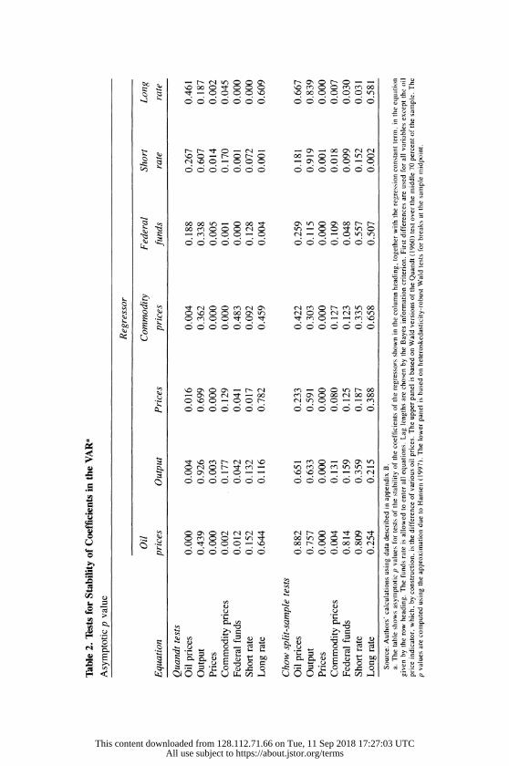
00 > Ic tr, oo t o om o o o --E
OC C t O) ' ) N0 r0-~f --
z~~~~~~ m s o m W') 00 ) "C O) O) OC ON O OOOOr) C L
,,C ON C) ON CA - tr -- -OC- ca NN c
- xD O - O 0 O m o00L 0 r = o- E N 0 o oo-o o
U Cq 00 0 m -O 00tr 00 t r o>>
~~ ~. 6666666 66 6666 %
0u
> t - o) O O O 2 - 4O t1 - r t ; 0 u u Ot O OOOOOO
U ~ ~ ~ ~~~~~~~~~~~~- U
C) > U>
0 0 U 0 U~~~~~~~~~~o
U CU'
'U O 0.-
>~~~~ CEc; o ooo o o o c,
S~~~X o
This content downloaded from 128.112.71.66 on Tue, 11 Sep 2018 17:27:03 UTCAll use subject to https://about.jstor.org/terms
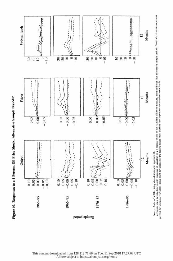
~~~~~~~~~I I 42 I I
C C C C) C C ) I I C C C c C - C
'0 I I I ii
. I ~I I I I I I I
C) ,C C)
;~~~~~~~~~~~~~~~~~~~~~~~~~~ 0:
_ O ~~ONOOO O?O? ON ON ONOOa
@ I II III I I I I *- n
O~~~~~~~~ I K. .I X ~ ~~ ~~ ~~ In .... I 0 5 e
Y J /0 .-t
pouad oldwuxS
This content downloaded from 128.112.71.66 on Tue, 11 Sep 2018 17:27:03 UTCAll use subject to https://about.jstor.org/terms

136 Brookings Papers on Economic Activity, 1:1997
response in the funds rate. The atypical behavior of the funds rate during
this period may reflect the presence of confounding factors, such as the
weakness of financial sector balance sheets and the decline in consumer
confidence that depressed the economy at the time of the one major oil
shock of that subsample, the 1990 increase in prices. In any event, the
subsample evidence is highly consistent with the view that the reduced-
form impact of oil on the economy depends significantly on the mone-
tary policy reaction function.
Conclusion
This paper offers both methodological and substantive contributions.
Methodologically, we show how to modify standard VAR systems to
permit simulations of the economy under alternative endogenous poli-
cies. Since our focus is on quantifying the economic impact of historical
feedback policies, the alternative policy that we consider is very simple;
a virtue of our approach is that it would not be difficult to extend the
analysis to consider more interesting alternatives, for example, "Taylor
rules." It would also be interesting to compare our results with those
obtained from alternative (possibly, more structural) methodologies.
Substantively, our results suggest that an important part of the effect
of oil price shocks on the economy results not from the change in oil
prices, per se, but from the resulting tightening of monetary policy.
This finding may help to explain the apparently large effects of oil price
changes found by Hamilton and many others.
APPENDIX A
Interpolation of Monthly NIPA Variables
IN THIS PAPER we use interpolated monthly values of GDP, the com-
ponents of GDP, and the GDP deflator. This appendix describes the
interpolation process. The data and additional detailed estimation re-
This content downloaded from 128.112.71.66 on Tue, 11 Sep 2018 17:27:03 UTCAll use subject to https://about.jstor.org/terms

Ben S. Bernanke, Mark Gertler, and Mark Watson 137
sults are available on a distribution diskette from the authors, upon
request.
We designate quarterly series by capital letters and monthly series
by lower-case letters. Quarters are indexed by T = 1, 2, ..., N, and
months by t = 1, 2, ..., n. Let QT be an (observed) quarterly variable
that is to be interpolated-for example, real GDP-and let ST be a
scaling variable such that YT QTIST is nontrending. Similarly, let q, be the (unobserved) monthly series corresponding to QT-for example,
montly real GDP-and let s, be a scaling variable such that y, q,/s, is nontrending. QT and q, are related by the identity
2
1 QT 3 - q3T-i,
and hence YT and y, are related by the identity
= 1 2
YT 3 Y3T_ i(S3T i/ST)
Interpolation is by state space methods. Suppose that there is a vector
of (observable) interpolator variables at the monthly level, x,; industrial
production, for example, is a monthly variable that provides informa-
tion about within-quarter movements of real GDP. We assume that the
unobserved monthly variable y, is related to the interpolator variables
according to the "causal," or "transition," equation
y,= x,' + u,,
where
u, = pu,_, + E,, E, - N(O,&2).
In our application, all transition equations include a constant term.
When one or more of the interpolators becomes available midsample,
all interpolators (including the constant term) are interacted with
dummy variables and the possibility of a shift in the value of .2 is allowed for.
Let z, be a monthly "indicator" variable that equals Y,,3 in the third
month of each quarter and is zero otherwise. Then the indicator, or
measurement, equations are given by
This content downloaded from 128.112.71.66 on Tue, 11 Sep 2018 17:27:03 UTCAll use subject to https://about.jstor.org/terms
138 Brookings Papers on Economic Activity, 1:1997
2
z,= E y,ti(s,tJlS3,), t = 3, 6, 9, 12, ...,n
and
z=0 x y,, for all other values of t.
The parameters p, p, and 02 are estimated by maximum likelihood, assuming Gaussian errors. Conditional on the estimated parameters, let
ytl, = E,yt, where E is the expectations operator. The interpolated values, given the full information set, are thus given by
qt,E = ytl,,st.
This method is similar to that proposed by Chow and Lin (1971),
although it allows for a more general treatment of the serial correlation
in u,.
To estimate the accuracy of the interpolation, one can use R2 mea-
sures of fit. In levels, the measure of fit is
R,eis = var(y2,,)/var(y2),
and in differences it is
R = var(zAy2,,)/var(zAy2).
Table Al lists the quarterly series that we interpolate, the corre-
sponding monthly interpolators, and the measures of fit (corresponding
to the scaled values of the variables). Variables are listed by their
CITIBASE mnemonics, which are defined in appendix B. The scale
variables used for real flow variables are personal consumption expen-
ditures (GMCQ), at both the quarterly and monthly levels. The personal
consumption expenditure deflator (GMDC), monthly and quarterly, is
used as the scale variable in the interpolation of the GDP deflator.
Consumption data (disaggregated to durables, nondurables, and ser-
vices) exist at a monthly frequency and thus do not have to be inter-
polated. Monthly GDP is calculated as the sum of the monthly GDP
components (we ignore the slight deviations from that relationship
caused by chain weighting).
The R2 values suggest that the interpolators explain nearly all of the
variability in the levels of the scaled series. With the exceptions of
government consumption and the GDP deflator, they also explain nearly all of the implied month-to-month variation in the series.
This content downloaded from 128.112.71.66 on Tue, 11 Sep 2018 17:27:03 UTCAll use subject to https://about.jstor.org/terms
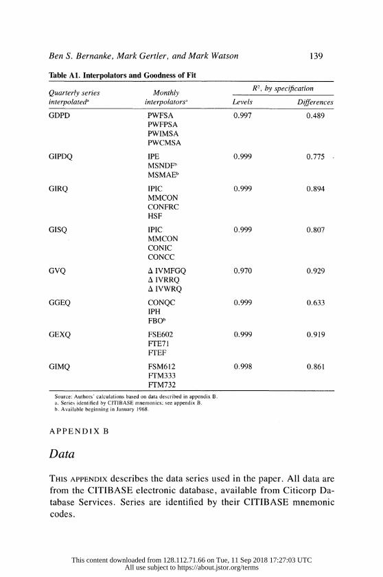
Ben S. Bernanke, Mark Gertler, and Mark Watson 139
Table Al. Interpolators and Goodness of Fit
Quarterly series Monthly R2, by specification
interpolateda interpolatorsa Levels Differences
GDPD PWFSA 0.997 0.489
PWFPSA
PWIMSA
PWCMSA
GIPDQ IPE 0.999 0.775
MSNDFb
MSMAEb
GIRQ IPIC 0.999 0.894
MMCON
CONFRC
HSF
GISQ IPIC 0.999 0.807
MMCON
CONIC
CONCC
GVQ A IVMFGQ 0.970 0.929 A IVRRQ
A IVWRQ
GGEQ CONQC 0.999 0.633 IPH
FBOb
GEXQ FSE602 0.999 0.919
FTE71
FTEF
GIMQ FSM612 0.998 0.861 FTM333
FTM732
Source: Authors' calculations based on data described in appendix B. a. Series identified by CITIBASE mnemonics, see appendix B. b. Available beginning in January 1968.
APPENDIX B
Data
THIS APPENDIX describes the data series used in the paper. All data are
from the CITIBASE electronic database, available from Citicorp Da-
tabase Services. Series are identified by their CITIBASE mnemonic
codes.
This content downloaded from 128.112.71.66 on Tue, 11 Sep 2018 17:27:03 UTCAll use subject to https://about.jstor.org/terms
140 Brookings Papers on Economic Activity, 1:1997
Quarterly series
GDPD GDP deflator, index, 1992 = 100.
GEXQ Exports of goods and services, chained 1992 dollars.
GGEQ Government consumption expenditures and gross investment,
chained 1992 dollars.
GIMQ Imports of goods and services, chained 1992 dollars.
GIPDQ Investment, producers' durables, chained 1992 dollars.
GIRQ Investment, residential, chained 1992 dollars.
GISQ Investment, nonresidential structures, chained 1992 dollars.
GVQ Change in business inventories, total, chained 1992 dollars.
Monthly series
CONCC Construction put in place, commercial, seasonally adjusted,
1987 dollars.
CONFRC Construction put in place, private residential building, season-
ally adjusted, 1987 dollars.
CONIC Construction put in place, industrial building, seasonally ad-
justed, 1987 dollars.
CONQC Construction put in place, public, seasonally adjusted, 1987
dollars.
FBO Federal budget, net outlay, not seasonally adjusted; deflated
by interpolated government purchases deflator (GDFGEC),
seasonally adjusted by the authors by means of a regression on
monthly dummies.
FSE602 Exports, excluding military aid shipments, seasonally adjusted;
deflated by the PPI for finished goods (PWF).
FSM612 General imports, seasonally adjusted; deflated by the PPI for
finished goods (PWF).
FTE71 U.S. merchandise exports, nonelectrical machinery, season-
ally adjusted; deflated by the PPI for machinery and equipment
(PWME).
This content downloaded from 128.112.71.66 on Tue, 11 Sep 2018 17:27:03 UTCAll use subject to https://about.jstor.org/terms

Ben S. Bernanke, Mark Gertler, and Mark Watson 141
FTEF U.S. merchandise exports, agricultural products, seasonally
adjusted; deflated by the PPI for farm products, processed
foods, and feeds (PWFPF).
FTM333 U.S. merchandise imports, petroleum, and petroleum prod-
ucts, seasonally adjusted; deflated by the PPI for crude petro-
leum (PW561).
FTM732 U.S. merchandise imports, automobiles and parts, seasonally
adjusted; deflated by the PPI for motor vehicles and equipment
(PWAUTO).
FYFF Federal funds rate, percent.
FYGM3 Interest rate, three-month Treasury bills from the secondary
market, percent.
FYGT5 Interest rate, five-year Treasury bonds, constant maturity, from
the secondary market, percent.
FYGT10 Interest rate, ten-year Treasury bonds, constant maturity, from
the secondary market, percent.
GMCQ Personal consumption expenditures, seasonally adjusted,
chained 1992 dollars.
GMCDQ Personal consumption expenditures, durables, seasonally ad-
justed, chained 1992 dollars.
GMCNQ Personal consumption expenditures, nondurables, seasonally
adjusted, chained 1992 dollars.
GMCSQ Personal consumption expenditures, services, seasonally ad-
justed, chained 1992 dollars.
GMDC Implicit price deflator, personal consumption expenditures, in-
dex, 1987 = 100.
HSF Housing starts, new private housing units, seasonally adjusted.
IP Industrial production index, total, seasonally adjusted, 1987
= 100.
IPE Industrial production index, business equipment, seasonally
adjusted, 1987 = 100.
This content downloaded from 128.112.71.66 on Tue, 11 Sep 2018 17:27:03 UTCAll use subject to https://about.jstor.org/terms
142 Brookings Papers on Economic Activity, 1:1997
IPH Industrial production index, defense and space equipment, sea-
sonally adjusted, 1987 = 100.
IPIC Industrial production index, construction supplies, seasonally
adjusted, 1987 = 100.
IVMFGQ Inventories, manufacturing, seasonally adjusted, chained 1992
dollars.
IVRRQ Manufacturing and trade inventories, retail trade, seasonally
adjusted, chained 1992 dollars.
IVWRQ Manufacturing and trade inventories, merchant wholesalers,
seasonally adjusted, chained 1992 dollars.
MMCON Manufacturing shipments, construction materials and supplies,
seasonally adjusted; deflated by the PPI for materials and com-
ponents for manufacturing (PWIMSM).
MSMAE Manufacturing shipments, machinery and equipment, season-
ally adjusted; deflated by the PPI for machinery and equipment
(PWME).
MSNDF Manufacturing shipments, nondefense capital goods indus-
tries, seasonally adjusted; deflated by the PPI for capital equip-
ment (PWFP).
PSCCOM Spot market price index, all commodities, from Commodity
Research Bureau, not seasonally adjusted, 1967 = 100.
PUNEW CPI-U, all items, seasonally adjusted, 1982-84 = 100.
PW561 PPI, crude petroleum, not seasonally adjusted, 1982 = 100.
PWFPSA PPI, capital equipment, seasonally adjusted, 1982 = 100.
PWFSA PPI, finished goods, seasonally adjusted, 1982 = 100.
PWIMSA PPI, intermediate materials, supplies, and components, sea-
sonally adjusted, 1982 = 100.
PWCMSA PPI, crude materials, seasonally adjusted, 1982 = 100.
This content downloaded from 128.112.71.66 on Tue, 11 Sep 2018 17:27:03 UTCAll use subject to https://about.jstor.org/terms
Comments and Discussion
Christopher A. Sims: The broad aim of this paper is to go beyond the
result, now widely confirmed in the empirical time-series literature on
monetary policy, that surprise changes in monetary policy are a minor
source of economic fluctuations. The nature of systematic reactions of
monetary policy to the state of the economy could be a major determi-
nant of the character of fluctuations, even though erratic disturbances
to monetary policy are not. The paper concludes that the evidence is
consistent with a major role for monetary policy; so large that, for
example, most of the observed output effects of oil price shocks would
disappear with a different monetary policy.
I agree with the main conclusion of the paper, but only because the
authors have been so careful in stating it. I would emphasize more than
they do how much uncertainty remains about the size of the real effects
of monetary policy. It remains possible for a skeptic to maintain the
view that the effects of both systematic and random shifts in monetary
policy are negligibly small. My comments therefore emphasize the
reasons to doubt that the effects of systematic monetary policy are large,
despite the paper's evidence to the contrary.
The authors pursue their aim by focusing attention primarily on the
reaction of the economy to surprise changes in oil prices. On the face
of it, this focus is appealing, because most economists believe that they
know roughly when large surprise changes in oil prices have occurred
and have little doubt that these changes were distinct from surprise
changes in monetary policy. Identification-separation of the inter-
pretable disturbance from other sources of variation in the data-there-
143
This content downloaded from 128.112.71.66 on Tue, 11 Sep 2018 17:27:03 UTCAll use subject to https://about.jstor.org/terms

144 Brookings Papers on Economic Activity, 1:1997
fore promises to be easier than it would be with other types of private
sector disturbances. This idea, it seems to me, has not turned out as well as one might have hoped.
In the first place, the intuition that historical oil price "shocks" are
well understood and easily identified is incorrect. Although Hamilton's
original work did not require elaborate filtering of the data, it appears that to extend it to the current time does require such filtering. In the
present paper, four different measures of oil price shocks are shown in
figure 2 to deliver four quite distinct estimated effects on the economy.
The authors choose to proceed with Hamilton's filtration of the oil price
data to generate their oil price shocks.
As the paper notes, the estimated effects of the oil price shock are
small: a 1 percent oil price shock-which, by the definition of the variable, is expected to lead to a fairly persistent change in the actual
level of oil prices-leads, in figure 4, only to a 0.02 percent response of the price level and a 0.025 percent output response at the peak of
the responses. This is the size of the pure supply-side effect on GDP
that one would expect if oil-related energy inputs had a 2 percent factor share, and most economists would expect estimated reduced-form ef- fects of oil price increases to be larger than that. (This assumes that domestic oil is treated correctly as a primary input and that imports of foreign oil are treated correctly as intermediate inputs in GDP account- ing, a perhaps dubious assumption.) It would be useful in assessing
these results to know both the response of the oil price level, as opposed
to the filtered variable, to this shock and the size of a one standard
deviation shock to the filtered oil price measure.
Furthermore, though taken from different models, both the first row of table 1 and the error bands in the bottom row of figure 2 show that
the responses of the variables to an oil shock could easily be zero and
yet still consistent with the data; one-standard-error bands about the responses barely clear zero. It is true that table 1 shows that the differ- ence in the response of the economy in the case where monetary policy
responds according to historical norms and the case where it pegs the interest rate is fairly sharply defined by the data and is in the direction
expected by the authors. But since the oil shock itself has turned out to
be something of a will-o'-the-wisp, the idea that economists' intuitive knowledge of the size and nature of oil shocks would help with identi-
fication ends up not having contributed much.
This content downloaded from 128.112.71.66 on Tue, 11 Sep 2018 17:27:03 UTCAll use subject to https://about.jstor.org/terms
Ben S. Bernanke, Mark Gertler, and Mark Watson 145
The paper also shows some results for "output" and "commodity
price" shocks. These are derived from the statistical model and are harder to interpret than oil shocks. The model gives them no interpre-
tation, except that they are different from and independent of monetary
policy shocks. But while these model-based shocks probably mix con-
ceptually distinct non-monetary policy influences on the economy, they
do have the advantage of having large effects and accounting for much
of the observed variance in the data. It is encouraging to see in figures
8 and 9 that the effects of systematic monetary policy as measured with
the oil shocks seem to be confirmed with the output and price shocks, but it is disappointing that all of the careful analysis of robustness and
statistical strength centers on the less sharply defined oil price shocks.
The authors point out that previous experiments with analyzing the effects of systematic changes in monetary policy in identified VAR
models have stuck to replacing the estimated policy rule in the model
with something else. This kind of exercise implicitly assumes that in
forming expectations of future policy actions, private agents treat all
deviations of policy variables from their historical patterns of behavior
as unsystematic deviations from the historical policy rule. The Lucas
critique warns that this can lead to error.
My own view of the Lucas critique is that it explains that it is always a mistake to imagine that one can implement changes in policy that
have probability zero according to the model of policy underlying pri-
vate sector behavior. The implication is that if one can contemplate
changing the coefficients of the "rule," or "reaction function," those coefficients should have been modeled as stochastic in the first place. There is an internal contradiction in pretending that one can change the
coefficients, even though the public is modeled as absolutely certain that they can never change.
While this point is correct in principle, it is difficult to implement in
practice. Especially for policy changes quite different from any that have been observed historically, estimation of an appropriate stochastic model that allows for such changes will be difficult and may need to
rely heavily on guesswork and a priori knowledge. It is therefore a good idea, where possible, to focus attention on policy changes that are not too dramatic, which can reasonably be modeled as sequences of random disturbances to the policy behavior that is explicit in the model. This
applies even when one is generating variations in policy by changing
This content downloaded from 128.112.71.66 on Tue, 11 Sep 2018 17:27:03 UTCAll use subject to https://about.jstor.org/terms
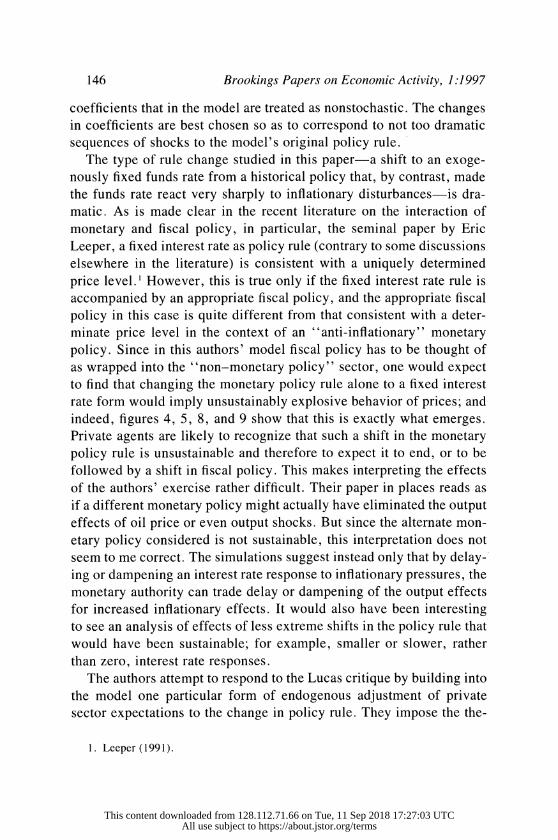
146 Brookings Papers on Economic Activity, 1:1997
coefficients that in the model are treated as nonstochastic. The changes
in coefficients are best chosen so as to correspond to not too dramatic
sequences of shocks to the model's original policy rule.
The type of rule change studied in this paper-a shift to an exoge-
nously fixed funds rate from a historical policy that, by contrast, made
the funds rate react very sharply to inflationary disturbances-is dra-
matic. As is made clear in the recent literature on the interaction of
monetary and fiscal policy, in particular, the seminal paper by Eric
Leeper, a fixed interest rate as policy rule (contrary to some discussions
elsewhere in the literature) is consistent with a uniquely determined
price level. ' However, this is true only if the fixed interest rate rule is
accompanied by an appropriate fiscal policy, and the appropriate fiscal
policy in this case is quite different from that consistent with a deter-
minate price level in the context of an "anti-inflationary" monetary
policy. Since in this authors' model fiscal policy has to be thought of
as wrapped into the "non-monetary policy" sector, one would expect
to find that changing the monetary policy rule alone to a fixed interest
rate form would imply unsustainably explosive behavior of prices; and
indeed, figures 4, 5, 8, and 9 show that this is exactly what emerges.
Private agents are likely to recognize that such a shift in the monetary
policy rule is unsustainable and therefore to expect it to end, or to be
followed by a shift in fiscal policy. This makes interpreting the effects
of the authors' exercise rather difficult. Their paper in places reads as
if a different monetary policy might actually have eliminated the output
effects of oil price or even output shocks. But since the alternate mon-
etary policy considered is not sustainable, this interpretation does not
seem to me correct. The simulations suggest instead only that by delay-
ing or dampening an interest rate response to inflationary pressures, the
monetary authority can trade delay or dampening of the output effects
for increased inflationary effects. It would also have been interesting
to see an analysis of effects of less extreme shifts in the policy rule that
would have been sustainable; for example, smaller or slower, rather
than zero, interest rate responses.
The authors attempt to respond to the Lucas critique by building into
the model one particular form of endogenous adjustment of private
sector expectations to the change in policy rule. They impose the the-
1. Leeper (1991).
This content downloaded from 128.112.71.66 on Tue, 11 Sep 2018 17:27:03 UTCAll use subject to https://about.jstor.org/terms
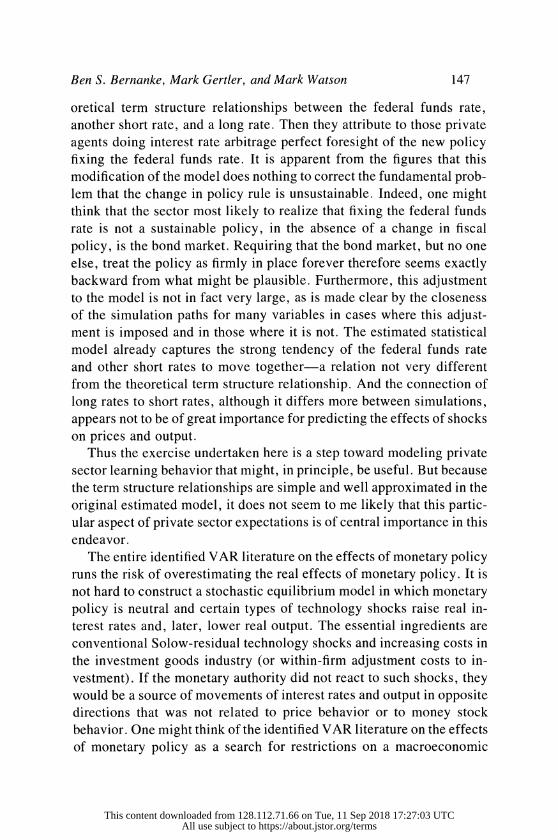
Ben S. Bernanke, Mark Gertler, and Mark Watson 147
oretical term structure relationships between the federal funds rate,
another short rate, and a long rate. Then they attribute to those private
agents doing interest rate arbitrage perfect foresight of the new policy
fixing the federal funds rate. It is apparent from the figures that this
modification of the model does nothing to correct the fundamental prob-
lem that the change in policy rule is unsustainable. Indeed, one might
think that the sector most likely to realize that fixing the federal funds
rate is not a sustainable policy, in the absence of a change in fiscal
policy, is the bond market. Requiring that the bond market, but no one
else, treat the policy as firmly in place forever therefore seems exactly
backward from what might be plausible. Furthermore, this adjustment
to the model is not in fact very large, as is made clear by the closeness
of the simulation paths for many variables in cases where this adjust-
ment is imposed and in those where it is not. The estimated statistical
model already captures the strong tendency of the federal funds rate
and other short rates to move together-a relation not very different
from the theoretical term structure relationship. And the connection of
long rates to short rates, although it differs more between simulations,
appears not to be of great importance for predicting the effects of shocks
on prices and output.
Thus the exercise undertaken here is a step toward modeling private
sector learning behavior that might, in principle, be useful. But because
the term structure relationships are simple and well approximated in the
original estimated model, it does not seem to me likely that this partic-
ular aspect of private sector expectations is of central importance in this
endeavor.
The entire identified VAR literature on the effects of monetary policy
runs the risk of overestimating the real effects of monetary policy. It is
not hard to construct a stochastic equilibrium model in which monetary
policy is neutral and certain types of technology shocks raise real in-
terest rates and, later, lower real output. The essential ingredients are
conventional Solow-residual technology shocks and increasing costs in
the investment goods industry (or within-firm adjustment costs to in-
vestment). If the monetary authority did not react to such shocks, they
would be a source of movements of interest rates and output in opposite
directions that was not related to price behavior or to money stock
behavior. One might think of the identified VAR literature on the effects
of monetary policy as a search for restrictions on a macroeconomic
This content downloaded from 128.112.71.66 on Tue, 11 Sep 2018 17:27:03 UTCAll use subject to https://about.jstor.org/terms
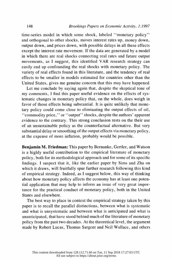
148 Brookings Papers on Economic Activity, 1:1997
time-series model in which some shock, labeled "monetary policy"
and orthogonal to other shocks, moves interest rates up, money down,
output down, and prices down, with possible delays in all these effects
except the interest rate movement. If the data are generated by a model
in which there are real shocks connecting real rates and future output
movements, as I suggest, this identified VAR research strategy can
easily end up confounding the real shocks with monetary policy. The
variety of real effects found in this literature, and the tendency of real
effects to be smaller in models estimated for countries other than the
United States, gives me genuine concern that this may have happened.
Let me conclude by saying again that, despite the skeptical tone of
my comments, I find this paper useful evidence on the effects of sys-
tematic changes in monetary policy that, on the whole, does weigh in
favor of those effects being substantial. It is quite unlikely that mone-
tary policy could come close to eliminating the output effects of oil,
"commodity price," or "output" shocks, despite the authors' apparent
evidence to the contrary. This strong conclusion rests on the their use
of an unsustainable policy as the counterfactual alternative. But very
substantial delay or smoothing of the output effects via monetary policy,
at the expense of more inflation, probably would be possible.
Benjamin M. Friedman: This paper by Bernanke, Gertler, and Watson
is a highly useful contribution to the empirical literature of monetary
policy, both for its methodological approach and for some of its specific
findings. I suspect that it, like the earlier paper by Sims and Zha on
which it draws, will fruitfully spur further research following this kind
of empirical strategy. Indeed, as I suggest below, this way of thinking
about how monetary policy affects the economy has at least one poten-
tial application that may help to inform an issue of very great impor-
tance for the practical conduct of monetary policy, both in the United
States and elsewhere.
The best way to place in context the empirical strategy taken by this
paper is to recall the parallel distinctions, between what is systematic
and what is unsystematic and between what is anticipated and what is
unanticipated, that have stood behind much of the literature of monetary policy from the past two decades. At the theoretical level, the argument
made by Robert Lucas, Thomas Sargent and Neil Wallace, and others
This content downloaded from 128.112.71.66 on Tue, 11 Sep 2018 17:27:03 UTCAll use subject to https://about.jstor.org/terms
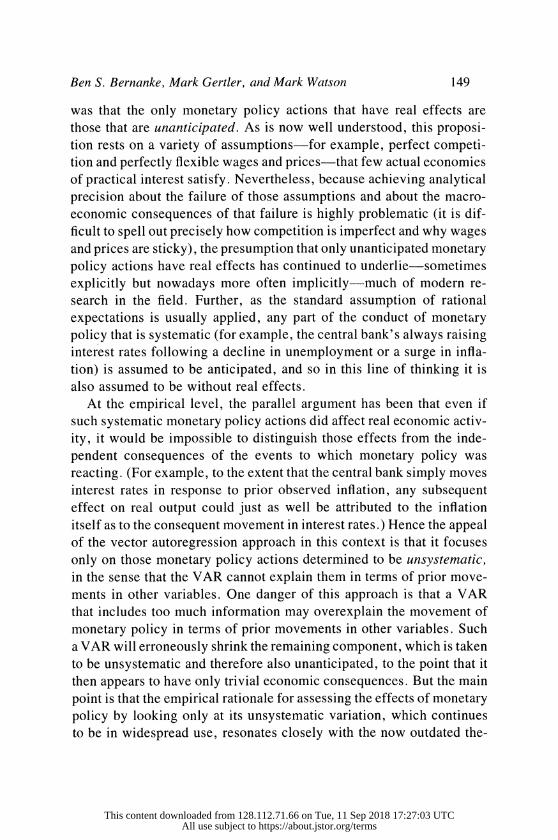
Ben S. Bernanke, Mark Gertler, and Mark Watson 149
was that the only monetary policy actions that have real effects are
those that are unanticipated. As is now well understood, this proposi-
tion rests on a variety of assumptions-for example, perfect competi-
tion and perfectly flexible wages and prices-that few actual economies
of practical interest satisfy. Nevertheless, because achieving analytical
precision about the failure of those assumptions and about the macro-
economic consequences of that failure is highly problematic (it is dif-
ficult to spell out precisely how competition is imperfect and why wages
and prices are sticky), the presumption that only unanticipated monetary
policy actions have real effects has continued to underlie-sometimes
explicitly but nowadays more often implicitly-much of modern re-
search in the field. Further, as the standard assumption of rational
expectations is usually applied, any part of the conduct of monetary
policy that is systematic (for example, the central bank's always raising
interest rates following a decline in unemployment or a surge in infla-
tion) is assumed to be anticipated, and so in this line of thinking it is
also assumed to be without real effects.
At the empirical level, the parallel argument has been that even if
such systematic monetary policy actions did affect real economic activ-
ity, it would be impossible to distinguish those effects from the inde-
pendent consequences of the events to which monetary policy was
reacting. (For example, to the extent that the central bank simply moves
interest rates in response to prior observed inflation, any subsequent
effect on real output could just as well be attributed to the inflation
itself as to the consequent movement in interest rates.) Hence the appeal
of the vector autoregression approach in this context is that it focuses
only on those monetary policy actions determined to be unsystematic,
in the sense that the VAR cannot explain them in terms of prior move-
ments in other variables. One danger of this approach is that a VAR
that includes too much information may overexplain the movement of
monetary policy in terms of prior movements in other variables. Such
a VAR will erroneously shrink the remaining component, which is taken
to be unsystematic and therefore also unanticipated, to the point that it
then appears to have only trivial economic consequences. But the main
point is that the empirical rationale for assessing the effects of monetary
policy by looking only at its unsystematic variation, which continues
to be in widespread use, resonates closely with the now outdated the-
This content downloaded from 128.112.71.66 on Tue, 11 Sep 2018 17:27:03 UTCAll use subject to https://about.jstor.org/terms

150 Brookings Papers on Economic Activity, 1:1997
oretical presumption that, at least for purposes of effects on real vari-
ables, only unanticipated policy actions matter. There is an inherent
congruence between the two lines of thinking.
The principal thrust of the approach taken by Bernanke, Gertler, and
Watson is to sever that connection by designing a way to use the em-
pirical VAR methodology to investigate specific aspects of systematic
monetary policy. To be sure, the paper simply presumes, rather than
shows, that systematic and therefore anticipated monetary policy ac-
tions can have real effects. But for readers who accept that there are
reasons why this may be so and who do not require that the empirical
model used to investigate these effects be explicitly tied to a theoretical
model detailing how they come about, the resulting advance is clear.
And indeed, the authors find that the specific aspect of systematic mon-
etary policy on which they choose to focus-the central bank's response
to oil price shocks and to the consequences of those shocks for prices
and output-does have sizable real effects. This finding is both inter-
esting and important. (To be clear, the within month response of mon-
etary policy to an oil price shock would be unanticipated and therefore
presumed to have real effects, even in a Lucas-style model. Although
the paper is not specific on this distinction, I assume that the bulk of
the real effects that the authors attribute to the monetary policy response
to oil price shocks results from movement in the policy variable occur-
ring after the month in which the oil price moves.)
As indicated at the outset, I suspect that this methodology has an
immediate application of potentially great importance. A question that
has rightly attracted widespread attention, among industrial as well as
developing countries, is how price inflation affects a country's ability
to maintain real economic growth. Evidence shows that above some
modest level (the high single-digit range), inflation does reduce the
average pace of real growth over time. A familiar view, however, is
that inflation negatively affects real growth not because inflation, per
se, matters in this context, but because the central bank acts to resist
inflation; and in a world in which the Lucas-Sargent-Wallace assump-
tions do not obtain, it can only do so by slowing ("sacrificing") real
output. The methodology used in this paper seems potentially able to
address this question too. If so, the findings would be very valuable.
Although both the methodology and the findings of Bernanke,
Gertler, and Watson's paper are highly useful, three specific aspects
This content downloaded from 128.112.71.66 on Tue, 11 Sep 2018 17:27:03 UTCAll use subject to https://about.jstor.org/terms
Ben S. Bernanke, Mark Gertler, and Mark Watson 151
give cause for reservation. First, as they are at some pains to emphasize,
there is substantial evidence of instability in their results across the
three decades of their sample. In particular, as figure 10 clearly shows,
the "systematic" response of monetary policy to oil price shocks in the
Volcker period was far greater than either earlier or later.
A question that this instability immediately raises is whether it is
reasonable to view the more energetic anti-inflationary monetary policy
of the Volcker era exclusively as a response to an oil price shock. I
believe that the Federal Reserve System under Paul Volcker adopted a
policy broadly aimed at reducing the U.S. inflation rate, and that the
rise in oil prices in 1979 and 1980 was only one element in the inflation
process against which it directed its policy. The results plotted in the
middle right-hand panel in figure 6, showing that the simulated response
to the historical oil shock accounts for only a small part of the increase
in the federal funds rate during 1981-82, are certainly consistent with
this view. Because of the post hoc ergo propter hoc character of VAR
analysis, the Bernanke-Gertler-Watson paper may attribute to the spe-
cific response (here and in other subperiods) of monetary policy to oil
price shocks what was actually the more general conduct of monetary
policy, based on other considerations.
The findings of subsample instability also highlight the difficulty of
identifying what "systematic" policy means in the first place. For
purely empirical purposes of extracting impulse responses and variance
decomparisons from past data, systematic simply means whatever hap-
pened on average across the arbitrarily chosen sample under study. But
as is the case in this paper, researchers often seek to connect this purely
empirical notion of systematic behavior with the concept of policy
"rules," so as to go on to draw inferences about the consequences of
the central bank following one rule rather than another. As a number
of people (Sims, John Taylor, and I, among many others) have argued
in one context or another, it is not clear that in practical settings the
central bank is ever following a rule, in the crucial dual sense that its
actions are not only systematic but also perceived to be so and therefore
properly anticipated by the relevant public. The fact that estimating the
authors' VAR over the 1976-85 sample delivers the federal funds rate
response shown in the right-hand panel of the third row in figure 10
does not necessarily make this response a characterization of systematic
monetary policy in any substantive sense.
This content downloaded from 128.112.71.66 on Tue, 11 Sep 2018 17:27:03 UTCAll use subject to https://about.jstor.org/terms
152 Brookings Papers on Economic Activity, 1:1997
A second set of reservations stems from the authors' use of oil price
shocks as the principal empirical vehicle for their study of systematic
monetary policy. To put it bluntly, does the Hamilton idea really make
sense? For example, should one really think of the 1957-58 recession
in the United States as a ripple from the 1956 Suez affair? To take
Hamilton's idea seriously would require a major rethinking of most of
post-World War II U.S. business cycle history-which clearly has not
happened in the decade and a half since Hamilton's intriguing paper
appeared. The authors of the present paper are perhaps more secure in
that the role of oil prices is more plausible in at least two, possibly
three, of the five recessions covered in their sample, which mostly
postdates Hamilton's. Even so, I suspect that their difficulty in finding
a measure of oil price shocks that satisfactorily fits the oil facts to the
macroeconomic data is a warning of just this problem.
Finally, several aspects of the authors' treatment of interest rates
also bear closer attention. The assumption that interest rate movements
are a sufficient statistic for the channels by which monetary policy
affects macroeconomic activity is, by itself, not unusual. Indeed, the
authors may well overemphasize its limitations. Costs of financing (in-
cluding opportunity costs) are an important factor in many kinds of
spending decisions, and for this purpose interest rate fluctuations may
also plausibly stand in for at least part of the relevant movement in
either exchange rates or broader asset prices. While the strong rejection
of the restriction excluding the federal funds rate from the output equa-
tion is somewhat surprising, the authors are presumably correct that the
practical effects of imposing this restriction are small. Further, it is my
conjecture that if a stock price index were included in the VAR, the
data would accept this restriction. (Because the analysis in this paper
depends so crucially on the role of short- and long-term interest rates, however, there is probably much to be learned from examining the
coefficients of these interest rates in the output equation, as well as the
impulse responses relating output to the independent components of the
two interest rates. It would therefore be useful to show explicitly these
key elements of the analysis.)
The potential problem, however, is the strong implied rejection of
the expectations hypothesis of the term structure of interest rates, which
the authors use as the organizing principle for this part of their model.
Normally, within this framework, the "term premium" included in any
This content downloaded from 128.112.71.66 on Tue, 11 Sep 2018 17:27:03 UTCAll use subject to https://about.jstor.org/terms
Ben S. Bernanke, Mark Gertler, and Mark Watson 153
specific interest rate is a substantive reflection of borrowers' and lend-
ers' attitudes toward such features as the risk and liquidity of the un-
derlying debt instrument. But in this paper, the term premium simply
serves to undo the behavior that the built-in expectations hypothesis
implies that interest rates should be following (see, for example, fig-
ure 3). Moreover, the results plotted in figure 4 for prices and the long-
term rate are dramatically at variance with standard notions of how
inflation expectations affect nominal interest rates. In this experiment,
not surprisingly, moving from the base simulation to either the Sims-
Zha simulation or the anticipated policy simulation results in far higher
prices and hence much greater inflation. But in the Sims-Zha simulation
the long-term interest rate is uniformly below its level in the base
simulation, and in the anticipated policy simulation it even declines
absolutely. So much for the notion that investors rationally anticipate
the consequences of monetary policy for future inflation and incorporate
the resulting inflation expectations into current bond prices!
These three sets of reservations notwithstanding, I applaud the
broader methodological direction taken by Bernanke, Gertler, and Wat-
son and retain my sense that their finding of quantitatively significant
effects from systematic monetary policy is both correct and important.
General discussion: Participants generally accepted the authors' con-
clusion that the output declines following oil price shocks had come
mainly from the responses of monetary policy to the shocks. Several
also discussed the plausible magnitude of oil shock effects themselves.
One issue was how much an oil price increase, or a decrease in oil
supply, should affect potential output; a second was whether oil price
increases reduce demand and lead to lower levels of utilization of pro-
ductive capacity. Robert Hall observed that, for infinitesimal changes
in oil prices, the ability of the United States to produce should not be
impaired by a rise in the price of imported oil, even if it reduces oil
use; the derivative of real GDP with respect to the price of oil is zero
no matter how large the adjustment, with Division GDP. However, he
and William Nordhaus agreed there could be effects on potential GDP
as the equilibrium supply of domestic factors adjusted to the change in
oil prices. George Perry added that some estimates from earlier studies,
such as a reduction of several percentage points of GDP from OPEC 1,
were too large to be viewed as a supply-side effect. However, taking
This content downloaded from 128.112.71.66 on Tue, 11 Sep 2018 17:27:03 UTCAll use subject to https://about.jstor.org/terms

154 Brookings Papers on Economic Activity, 1:1997
into account the effect of an oil price increase on aggregate demand, where
the price increase could be analyzed approximately like an increase in
excise taxes with high-saving foreigners getting the revenue, a large short-
run impact on GDP was believable. He added that the allocation of such
an impact between a "fiscal" and a monetary effect would depend, some-
what arbitrarily, on how baseline monetary policy was defined.
Nordhaus raised several issues about the appropriateness of the var-
ious measures of oil shocks used by the authors. He suggested that
almost any theory, whether Perry's that the short-run impact of in-
creases could be regarded as a tax paid to foreigners or Sims's that it
should be treated simply as an increase in input prices, should lead to
some measure involving oil purchases relative to the size of the econ-
omy. This scaling makes an enormous difference. For the last three oil
shocks in the sample, he calculated the increased costs of imported oil,
with quantities fixed, were 1.8 percent of GDP in 1973, 1.0 percent of
GDP in 1979, and 0.2 percent of GDP in 1990. Using this measure
would preserve the peaks of the Hamilton series, but the shocks would
be progressively smaller. Nordhaus also noted that the paper ignores
the negative oil shock of 1986, when the price decline corresponded to
a negative shock of 0.5 percent of GDP. He reasoned that the failure to
scale the shocks, along with the fact that the positive shocks of 1986 and
1990 were quickly reversed, may explain why the responses in the two
subperiods look so different in the authors' analysis. William Brainard
agreed with Nordhaus's argument for scaling the shocks and added that it
might be useful to construct a similar measure indicating the magnitude
of the redistribution between domestic producers and consumers.
Robert Shiller observed that the stochastic properties of the oil price
series seemed to have changed after the Organization of Petroleum
Exporting Countries broke up in 1986. Before that, the oil price was a
series of plateaus separated by sudden jumps, so that changes seem to
have a lot of information. But afterward, the oil price looks like a mean-
reverting process, so the movements have less information. He reasoned
that the public may realize this difference, which would explain why
oil price changes are no longer big news. Reflecting on the widespread
concerns about oil in the 1970s and 1980s, Shiller suggested that the
long view is important in economics and the best way to deal with an
anomaly is to wait it out until it disappears. He suggested that may have
happened with oil.
This content downloaded from 128.112.71.66 on Tue, 11 Sep 2018 17:27:03 UTCAll use subject to https://about.jstor.org/terms

Ben S. Bernanke, Mark Gertler, and Mark Watson 155
References
Andersen, Leonall C., and Jerry L. Jordan. 1968. "Monetary and Fiscal Ac-
tions: A Test of Their Relative Importance in Economic Stabilization."
Federal Reserve Bank of St. Louis Review (November): 11-24.
Bernanke, Ben S., and Alan S. Blinder. 1992. "The Federal Funds Rate and
the Channels of Monetary Transmission." American Economic Review
82(4): 901-21.
Bernanke, Ben S., and Ilian Mihov. 1995. "Measuring Monetary Policy."
Working Paper 5145. Cambridge, Mass.: National Bureau of Economic
Research (June).
Blanchard, Olivier J. 1984. "The Lucas Critique and the Volcker Deflation." American Economic Review, Papers and Proceedings 74(2): 211-15.
Chow, Gregory, and An-loh Lin. 1971. "Best Linear Unbiased Interpolation, Distribution, and Extrapolation of Time Series by Related Series." Review
of Economics and Statistics 53(4): 372-5.
Christiano, Lawrence J., and Martin Eichenbaum. 1992. "Identification and
the Liquidity Effect of a Monetary Policy Shock." In Political Economy,
Growth, and Business Cycles, edited by Alex Cukierman, Zvi Hercovitz, and Leonardo Leiderman. MIT Press.
Cochrane, John H. 1996. "What Do the VARs Mean? Measuring the Output Effects of Monetary Policy" Unpublished paper, University of Chicago
(August).
Darby, Michael R. 1982. "The Price of Oil and World Inflation and Reces-
sion. " American Economic Review 72(4): 738-51.
Dotsey, Michael, and Max Reid. 1992. "Oil Shocks, Monetary Policy, and
Economic Activity." Federal Reserve Bank of Richmond Economic Review
78(4): 14-27.
Ferderer, J. Peter. 1996. "Oil Price Volatility and the Macroeconomy." Jour-
nal of Macroeconomics 18(1): 1-26.
Friedman, Benjamin M., and Kenneth N. Kuttner. 1996. "A Price Target for
U.S. Monetary Policy? Lessons from the Experience with Money Growth Targets." BPEA, 1:1996, 77-125.
Friedman, Milton, and Anna Jacobson Schwartz. 1963. A Monetary History of the United States, 1867-1960. Princeton University Press.
Fuhrer, Jeffrey C. 1996. "Monetary Policy Shifts and Long-Term Interest Rates." Quarterly Journal of Economics 111(4): 1183-209.
Hamilton, James D. 1983. "Oil and the Macroeconomy Since World War II." Journal of Political Economy 91(2): 228-48.
. 1996a. "Analysis of the Transmission of Oil Price Shocks Through the Macroeconomy." Unpublished paper. University of California, San Diego (August).
This content downloaded from 128.112.71.66 on Tue, 11 Sep 2018 17:27:03 UTCAll use subject to https://about.jstor.org/terms
156 Brookin2s Pavers on Economic Activity. 1:1997
. 1996b. "This is What Happened to the Oil Price-Macroeconomy
Relationship." Journal of Monetary Economics 38(2): 215-20.
Hansen, Bruce E. 1997. "Approximate Asymptotic P Values for Structural-
Change Tests." Journal of Business and Economic Statistics 15(1): 60-67.
Hooker, Mark A. 1996a. "Exploring the Robustness of the Oil Price-
Macroeconomy Relationship: Empirical Specifications and the Role of Mon-
etary Policy." Unpublished paper. Wellesley College (September).
. 1996b. "What Happened to the Oil Price-Macroeconomy Relation-
ship?" Journal of Monetary Economics 38(2): 195-213.
Hoover, Kevin D., and Stephen J. Perez. 1994. "Post Hoc Ergo Propter Hoc
Once More: An Evaluation of 'Does Monetary Policy Matter?' in the Spirit of James Tobin." Journal of Monetary Economics 34(1): 47-73.
Kim, In-Moo, and Prakash Loungani. 1992. "The Role of Energy in Real Business Cycle Models." Journal of Monetary Economics 29(2): 173-89.
Kim, Soyoung. 1995. "Does Monetary Policy Matter in the G-6 Countries? Using Common Identifying Assumptions About Monetary Policy Across Countries." Unpublished paper. Yale University (January).
Lee, Kiseok, Shawn Ni, and Ronald A. Ratti. 1995. "Oil Shocks and the Macroeconomy: The Role of Price Variability." Energy Journal 16(4): 39-56.
Leeper, Eric M. 1991. "Equilibria Under 'Active' and 'Passive' Monetary and Fiscal Policies." Journal of Monetary Economics 27(February): 129-47.
Leeper, Eric M., Christopher A. Sims, and Tao Zha. 1996. "What Does Monetary Policy Do?" BPEA, 2:1996, 1-63.
Lucas, Robert E. Jr. 1976. "Econometric Policy Evaluation: A Critique." Carnegie-Rochester Conference Series on Public Policy 1: 19-46.
Mork, Knut Anton. 1989. "Oil and the Macroeconomy When Prices Go Up and Down: An Extension of Hamilton's Results." Journal of Political Econ- omy 97(3): 740-44.
Quandt, Richard E. 1960. "Tests of the Hypothesis that a Linear Regression System Obeys Two Separate Regimes." Journal of the American Statistical Association 55(290): 324-30.
Romer, Christina D., and David H. Romer. 1989. "Does Monetary Policy Matter? A New Test in the Spirit of Friedman and Schwartz." In NBER Macroeconomics Annual 1989, edited by Olivier Jean Blanchard and Stanley Fischer. MIT Press.
Rotemberg, Julio J., and Michael Woodford. 1996. "Imperfect Competition and the Effects of Energy Price Increases on Economic Activity." Journal of Money, Credit, and Banking 28(4, part 1): 549-77.
Shapiro, Matthew D. 1994. "Federal Reserve Policy: Cause and Effect." In Monetary Policy, edited by N. Gregory Mankiw. University of Chicago Press.
This content downloaded from 128.112.71.66 on Tue, 11 Sep 2018 17:27:03 UTCAll use subject to https://about.jstor.org/terms
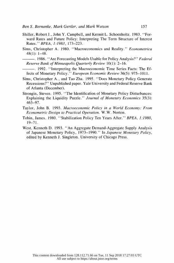
Ben S. Bernanke, Mark Gertler, and Mark Watson 157
Shiller, Robert J., John Y. Campbell, and Kermit L. Schoenholtz. 1983. "For-
ward Rates and Future Policy: Interpreting The Term Structure of Interest
Rates." BPEA, 1:1983, 173-223.
Sims, Christopher A. 1980. "Macroeconomics and Reality." Econometrica
48(1): 1-48.
. 1986. "Are Forecasting Models Usable for Policy Analysis?" Federal
Reserve Bank of Minneapolis Quarterly Review 10(1): 2-16.
. 1992. "Interpreting the Macroeconomic Time Series Facts: The Ef-
fects of Monetary Policy." European Economic Review 36(5): 975-1011.
Sims, Christopher A., and Tao Zha. 1995. "Does Monetary Policy Generate
Recessions?" Unpublished paper. Yale University and Federal Reserve Bank
of Atlanta (December).
Strongin, Steven. 1995. "The Identification of Monetary Policy Disturbances: Explaining the Liquidity Puzzle." Journal of Monetary Economics 35(3):
463-97.
Taylor, John B. 1993. Macroeconomic Policy in a World Economy: From Econometric Design to Practical Operation. W.W. Norton.
Tobin, James. 1980. "Stabilization Policy Ten Years After." BPEA, 1:1980,
19-71.
West, Kenneth D. 1993. "An Aggregate Demand-Aggregate Supply Analysis
of Japanese Monetary Policy, 1973-1990." In Japanese Monetary Policy,
edited by Kenneth J. Singleton. University of Chicago Press.
This content downloaded from 128.112.71.66 on Tue, 11 Sep 2018 17:27:03 UTCAll use subject to https://about.jstor.org/terms


![Advanced Macro: Bernanke, Gertler, and Gilchrist (1999 ...esims1/bbg_ers_notes_final.pdf · The expected return on holding capital from tto t+ 1 is: E t[Rk t+1] = E t RR t+1 + (1](https://img.pdfslide.us/doc/110x75/5f372d25c0505423dd414323/advanced-macro-bernanke-gertler-and-gilchrist-1999-esims1bbgersnotesfinalpdf.jpg)