University of RichmondUR Scholarship Repository

Physics Faculty Publications Physics

7-1-2013

Systematic Effects in Interferometric Observationsof the Cosmic Microwave Background PolarizationAta Karakci

Le Zhang

P. M. Sutter

Emory F. BunnUniversity of Richmond, ebunn@richmond.edu

Andrei Korotkov

See next page for additional authors

Follow this and additional works at: http://scholarship.richmond.edu/physics-faculty-publications

Part of the Atomic, Molecular and Optical Physics Commons

This Article is brought to you for free and open access by the Physics at UR Scholarship Repository. It has been accepted for inclusion in PhysicsFaculty Publications by an authorized administrator of UR Scholarship Repository. For more information, please contactscholarshiprepository@richmond.edu.

Recommended CitationKarakci, Ata, Le Zhang, P. M. Sutter, Emory F. Bunn, Andrei Korotkov, Peter Timbie, Gregory S. Tucker, and Benjamin D. Wandelt."Systematic Effects in Interferometric Observations of the Cosmic Microwave Background Polarization." The Astrophysical JournalSupplement Series 207, no. 1 ( July 01, 2013): 1-14. doi:10.1088/0067-0049/207/1/14.

AuthorsAta Karakci, Le Zhang, P. M. Sutter, Emory F. Bunn, Andrei Korotkov, Peter Timbie, Gregory S. Tucker, andBenjamin D. Wandelt

This article is available at UR Scholarship Repository: http://scholarship.richmond.edu/physics-faculty-publications/14

The Astrophysical Journal Supplement Series, 207:14 (14pp), 2013 July doi:10.1088/0067-0049/207/1/14C© 2013. The American Astronomical Society. All rights reserved. Printed in the U.S.A.

SYSTEMATIC EFFECTS IN INTERFEROMETRIC OBSERVATIONS OF THECOSMIC MICROWAVE BACKGROUND POLARIZATION

Ata Karakci1, Le Zhang2, P. M. Sutter3,4,5,6, Emory F. Bunn7, Andrei Korotkov1,Peter Timbie2, Gregory S. Tucker1, and Benjamin D. Wandelt3,4,5,8

1 Department of Physics, Brown University, 182 Hope Street, Providence, RI 02912, USA; ata_karakci@brown.edu2 Department of Physics, University of Wisconsin, Madison, WI 53706, USA

3 Department of Physics, 1110 W. Green Street, University of Illinois at Urbana-Champaign, Urbana, IL 61801, USA4 UPMC Univ. Paris 06, UMR 7095, Institut d’Astrophysique de Paris, 98 bis, boulevard Arago, F-75014 Paris, France

5 CNRS, UMR 7095, Institut d’Astrophysique de Paris, 98 bis, boulevard Arago, F-75014 Paris, France6 Center for Cosmology and Astro-Particle Physics, Ohio State University, Columbus, OH 43210, USA

7 Physics Department, University of Richmond, Richmond, VA 23173, USA8 Department of Astronomy, University of Illinois at Urbana-Champaign, Urbana, IL 61801, USA

Received 2013 February 26; accepted 2013 May 22; published 2013 July 2

ABSTRACT

The detection of the primordial B-mode spectrum of the polarized cosmic microwave background (CMB) signalmay provide a probe of inflation. However, observation of such a faint signal requires excellent control of systematicerrors. Interferometry proves to be a promising approach for overcoming such a challenge. In this paper we present acomplete simulation pipeline of interferometric observations of CMB polarization, including systematic errors. Weemploy two different methods for obtaining the power spectra from mock data produced by simulated observations:the maximum likelihood method and the method of Gibbs sampling. We show that the results from both methodsare consistent with each other as well as, within a factor of six, with analytical estimates. Several categories ofsystematic errors are considered: instrumental errors, consisting of antenna gain and antenna coupling errors; andbeam errors, consisting of antenna pointing errors, beam cross-polarization, and beam shape (and size) errors.In order to recover the tensor-to-scalar ratio, r, within a 10% tolerance level, which ensures the experiment issensitive enough to detect the B-signal at r = 0.01 in the multipole range 28 < � < 384, we find that, for aQUBIC-like experiment, Gaussian-distributed systematic errors must be controlled with precisions of |grms| = 0.1for antenna gain, |εrms| = 5 × 10−4 for antenna coupling, δrms ≈ 0.◦7 for pointing, ζrms ≈ 0.◦7 for beam shape, andμrms = 5 × 10−4 for beam cross-polarization. Although the combined systematic effects produce a tolerance levelon r twice as large for an experiment with linear polarizers, the resulting bias in r for a circular experiment is 15%which is still on the level of desirable sensitivity.

Key words: cosmic background radiation – cosmology: observations – instrumentation: interferometers –methods: data analysis – techniques: polarimetric

1. INTRODUCTION

The cosmic microwave background (CMB) has become oneof the most fundamental tools in cosmology. High-precisionmeasurements of the CMB polarization, especially detectingthe primordial “B-mode” polarization signals (Kamionkowskiet al. 1997), will represent a major step toward understand-ing the extremely early universe. These B-modes are generatedby primordial gravitational waves. A detection of these signalswould probe the epoch of inflation and place an important con-straint on the inflationary energy scale (Hu & Dodelson 2002). Inaddition, the secondary B-modes induced by gravitational lens-ing encode information about the distribution of dark matter.However, the B-mode signals are expected to be extremelysmall and current experiments can only place upper limits(Hinshaw et al. 2012) on the tensor-to-scalar ratio; the questfor the B-modes is a tremendous experimental challenge.

Due to the weakness of the B-mode signals—the largestsignal of the primordial B-modes is predicted to be less than0.1 μK—exquisite systematic error control is crucial for de-tecting and characterizing them. Compared to imaging systems,interferometers offer certain advantages for controlling system-atic effects because: (1) an interferometer does not require rapidchopping and scanning (Timbie et al. 2006) and, with simple op-tics, interferometric beam patterns have extremely low sidelobesand can be well understood, (2) interferometers are insensitive

to any uniform sky brightness or fluctuations in atmosphericemissions on scales larger than the beam width, (3) withoutdifferencing the signal from separate detectors, interferometersmeasure the Stokes parameters directly and inherently avoid theleakage from temperature into polarization (Bunn 2007) causedby mismatched beams and pointing errors, which are seriousproblems for B-mode detection with imaging experiments (Huet al. 2003; Su et al. 2011; Miller et al. 2009; O’Dea et al. 2007;Shimon et al. 2008; Yadav et al. 2010; Takahashi et al. 2010),(4) for observations of small patches of sky,9 E–B mode separa-tion would be cleaner in the Fourier domain for interferometricdata than in real-space (Park & Ng 2004), and (5) with the useof redundant baselines, systematic errors can be averaged out.In addition, they offer a straightforward way to determine theangular power spectrum since the output of an interferometer isthe visibility, that is, the Fourier transform of the sky intensityweighting by the response of the antennas.

Interferometers have proved to be powerful tools for studyingthe CMB temperature and polarization power spectra. In fact,DASI (Kovac et al. 2002) was the first instrument to detectthe faint CMB polarization anisotropies. Pioneering attempts tomeasure the CMB temperature anisotropy with interferometerswere made in the 1980s (Martin et al. 1980; Fomalont et al. 1984;

9 Ng (2005) discusses interferometric data with a small primary beam on thefull sky.

1

The Astrophysical Journal Supplement Series, 207:14 (14pp), 2013 July Karakci et al.

Knoke et al. 1984; Partridge et al. 1988; Timbie & Wilkinson1988). Several groups have successfully detected the CMBanisotropies. The Cosmic Anisotropy Telescope (CAT) was thefirst interferometer to actually detect structures in the CMB(O’Sullivan et al. 1995; Scott et al. 1996; Baker et al. 1999).The Cosmic Background Imager (CBI; Pearson et al. 2003)and the Very Small Array (VSA; Dickinson et al. 2004; Graingeet al. 2003) have detected the CMB temperature and polarizationangular power spectra down to sub-degree scales. In the nextfew years, the QUBIC instrument (Qubic Collaboration et al.2011) based on the novel concept of bolometric interferometryis expected to constrain the tensor-to-scalar ratio to 0.01 at the90% confidence level, with 1 yr of observing.

On the theory side, the formalism for analyzing interfero-metric CMB data has been well-developed (White et al. 1999;Hobson & Maisinger 2002; Park et al. 2003; Myers et al. 2003,2006; Hobson & Magueijo 1996). A pioneering study of system-atic effects for interferometers based on an analytic approachhas been performed by Bunn (2007). However, this approach isof course only a first-order approximation for assessing system-atics, since many important effects, such as the configuration ofthe array, instrumental noise, and the sampling variance due tofinite sky coverage and incomplete uv coverage, are not takeninto account. Any actual experiment therefore will naturally re-quire a complete simulation to assess exactly how systematiceffects bias the power spectrum recovery. In this respect, Zhanget al. (2012) have presented a simulation pipeline to assess thesystematic errors, mainly focusing on pointing errors. With a fullmaximum likelihood (ML) analysis of mock data, the simulationagrees with the analytical estimates and finds that, for QUBIC-like experiments, the Gaussian-distributed pointing errors haveto be controlled to the sub-degree level to avoid contaminatingthe primordial B-modes with r � 0.01.

Nevertheless, a comprehensive and complete analysis of var-ious systematic errors on CMB power spectrum measurementshas not been undertaken so far. In this paper, therefore, weperform a detailed study to completely diagnose the most seri-ous systematic effects including gain errors, cross-talk, cross-polarization, beam shape errors, and pointing errors, on theentire set of CMB temperature and polarization power spectra.In order to assess the effect of the systematic errors on B-modedetection and set allowable tolerance levels for those errors, weperform simulations for a specific interferometric observationwith an antenna configuration similar to the QUBIC instrument.We also extend the analytical expressions (Bunn 2007) for char-acterizing systematic effects on the full CMB power spectra.

For verifying the power spectrum analysis, we employ twocompletely independent codes based on the Gibbs sampling(GS) algorithm and the ML technique. The use of GS-basedBayesian inference with interferometric CMB observations hasbeen successfully demonstrated by Sutter et al. (2012) andKarakci et al. (2013). It allows extraction of the underlyingCMB power spectra and reconstruction of the pure CMB signalssimultaneously, with a much lower computational complexity incontrast to the traditional ML technique (Hobson & Maisinger2002).

In this paper, for given input CMB angular power spectra,we simulate the observed Stokes visibilities in the flat-skyapproximation. We believe that the flat-sky simulations aresufficiently accurate for the study of systematic errors. First, inour simulation, we assume single pointing observations with 5◦beam width, corresponding to a sky coverage fraction of fsky =0.37%. This sky patch is small enough to permit the use of the

flat-sky approximation. Second, all the data analysis processesare established using the flat-sky approximation while the mockvisibility data are also simulated using this approximation.Therefore, a self-consistent analysis is performed. However,when using a patch cut from the projection of spherical sky ontoa flat image as an “input” map, one should take into accountthe contamination (Bunn 2011) of “ambiguous” modes arisingfrom incomplete sky coverage and thus requires an appropriatedata analysis method to apply to this situation.

This paper is organized as follows. In Section 2, we brieflysummarize the effects of a variety of systematic errors on in-terferometric CMB observations and describe the analyticalmethod for estimating those errors. In Section 3, we describe thesimulations’ interferometric visibilities which include system-atic errors. In Section 4, we review the data analysis methodsused in this paper, including the GS technique and the ML ap-proach. In Section 5, we assess the systematic effects on theCMB power spectra. Finally, a discussion and summary aregiven in Section 6. The Appendix contains the complete ana-lytical expressions for the systematic effects on the full CMBpower spectra.

2. SYSTEMATICS

2.1. Instrument Errors and Beam Errors

In a polarimetric experiment, the Stokes parameters I,Q,Uand V can be obtained by using either linear or circularpolarizers. For a given baseline ujk = xk − xj , xk being theposition vector of the kth antenna, the visibilities can be writtenas a 2 × 2 matrix Vjk (Bunn 2007);

Vjk =∫

d2rAk(r)R · S · R−1A†j (r)e−2πiujk ·r, (1)

where the 2 × 2 matrix Ak(r) is the antenna pattern and

S =(

I + Q U + iVU − iV I − Q

). (2)

For a linear experiment, R is the identity matrix and for a circularexperiment,

R(circ) = 1√2

(1 i1 −i

). (3)

Various systematic errors can be modeled in the definition ofthe antenna pattern as follows (Bunn 2007)

Ak(r) = Jk · R · Aks (r) · R−1 (4)

where the Jones matrix Jk represents the instrumental errors,such as gain errors and antenna couplings. The matrix Ak

s is theantenna pattern that models the beam errors, such as pointingerrors, beam shape errors and cross-polarization. In an idealexperiment Jk = I, where I is the identity matrix, and theantenna pattern is given as Ak

s (r) = A(r)I, where A(r) is acircular Gaussian function.

In this paper we will consider only two types of instrumentalerrors; antenna gain, parameterized by gk

1 and gk2 , and couplings,

parameterized by εk1 and εk

2 . The coupling errors are caused bymixing of the two orthogonally polarized signals in the system.To account for the phase delays, the parameters g and ε are givenas complex numbers. The Jones matrix for the kth antenna canbe written as (Bunn 2007)

Jk =(

1 + gk1 εk

1

εk2 1 + gk

2

). (5)

2

The Astrophysical Journal Supplement Series, 207:14 (14pp), 2013 July Karakci et al.

For the beam errors, we will consider that each antennahas a slightly different beam width, ellipticity (beam shapeerrors), and beam center (pointing errors), as well as a cross-polar antenna response described by off-diagonal entries in theantenna pattern matrix (Bunn 2007);

Aks = Ak

0(ρ, φ)

(1 + 1

2μkρ2

σ 2 cos 2φ 12μk

ρ2

σ 2 sin 2φ

12μk

ρ2

σ 2 sin 2φ 1 − 12μk

ρ2

σ 2 cos 2φ

),

(6)where Ak

0(ρ, φ) is an elliptical Gaussian function written inpolar coordinates (ρ, φ), σ is the width of the ideal beam andμk is the cross-polarization parameter of the kth antenna. Thisparticular form of cross-polarization occurs, with μk = σ 2/2,when the curved sky patch is projected onto a plane.

2.2. Control Levels

The effect of errors on the power spectra can be described bythe root-mean-square difference between the actual spectrum,CXY

actual, which is recovered from the data of an experiment withsystematic errors, and the ideal spectrum, CXY

ideal, which wouldhave been recovered from the data of an experiment with nosystematic errors;

ΔCXY =⟨(

CXYactual − CXY

ideal

)2⟩1/2

(7)

where X, Y = {T ,E,B}.The strength of the effect of systematics can be quantified by

a tolerance parameter αXY defined by (O’Dea et al. 2007; Milleret al. 2009; Zhang et al. 2012)

αXY = ΔCXY

σXYstat

(8)

where σXYstat is the statistical 1σ error in the XY -spectrum of the

ideal experiment with no systematic errors.The main interest in a B-mode experiment is the tensor-to-

scalar ratio r which can be estimated as (O’Dea et al. 2007)

r =∑

b ∂rCBBb

(CBB

b − CBBb,lens

)/(σBB

b,stat

)2∑b

(∂rC

BBb /σBB

b,stat

)2 (9)

where b denotes the power band, CBBb,lens is the B-mode spectrum

due to weak gravitational lensing and CBBb depends linearly on r

through the amplitude of the primordial B-modes. The toleranceparameter of r is given by αr = Δr/σr (O’Dea et al. 2007);

Δr =∑

b αBBb

(∂rC

BBb /σBB

b,stat

)∑b

(∂rC

BBb /σBB

b,stat

)2 , (10a)

σr =(∑

b

(∂rC

BBb /σBB

b,stat

)2

)−1/2

. (10b)

For good control of systematics, the value of αr is required tostay below a determined tolerance limit.

2.3. Analytical Estimations

Analytical estimations of the effect of systematic errors onthe polarization power spectra are extensively examined in

Bunn (2007). Defining a vector of visibilities v = (VI , VQ, VU )corresponding to a single baseline u pointing in the x direction,for an ideal experiment, we can write

〈|VI |2〉 = CT T�=2πu, (11a)

〈|VQ|2〉 = CEE�=2πuc

2 + CBB�=2πus

2, (11b)

〈|VU |2〉 = CEE�=2πus

2 + CBB�=2πuc

2, (11c)

〈VQV ∗U 〉 = CEB

�=2πu(c2 − s2), (11d)

〈VIV∗Q〉 = CT E

�=2πuc, (11e)

〈VIV∗U 〉 = CT B

�=2πuc. (11f)

where c2, s2 and c are averages of cos2(2φ), sin2(2φ) and cos(2φ)over the beam patterns:

s2 =∫ |A2(k − 2πu)|2 sin2(2φ)d2k∫ |A2(k)|2d2k

= 1 − c2, (12)

where A2 is the Fourier transform of the ideal beam patternsquared. The unbiased estimator for CXY = 〈CXY 〉 is obtainedas

CXY = v† · NXY · v (13)

where NXY is a 3 × 3 matrix involving s2 and c (see theAppendix). For a baseline pointing in an arbitrary directionthe analysis is done in a rotated coordinate system:

vrot =(

1 0 00 cos 2θ sin 2θ0 − sin 2θ cos 2θ

)v, (14)

θ being the angle between u and the x-axis.The effect of errors on visibilities can be described, to first

order, by vactual = videal + δv. Combining videal and δv into asix-dimensional vector w = (v, δv), we can write the first orderapproximation as (Bunn 2007)(

ΔCXYrms

)2 = T r[(NXY · Mw)2] + (T r[NXY · Mw])2, (15)

where Mw = 〈w · w†〉 is the covariance matrix of w and

NXY =(

0 NXY

NXY 0

). (16)

The error on a particular band power is, then, given as anexpansion in terms of ideal power spectra:(

ΔCXYrms,b

)2 = p2rms

∑I,J

κ2XY,I,J CI

bCJb (17)

where p is the parameter that characterizes the error, suchas gain, g, coupling, ε, or cross-polarization, μ, and I, J ={T T , T E,EE,BB}. This expression is valid for a singlebaseline. For a system with nb baselines in band b, ΔCXY

rms,bmust be normalized by 1/

√nb, assuming there is no correlation

between error parameters of different baselines. Analyticalestimations of the coefficients κ2

XY,I,J for various systematicerrors are presented in the Appendix.

3

The Astrophysical Journal Supplement Series, 207:14 (14pp), 2013 July Karakci et al.

-40 -20 0 20 40 60

u [λ]

-40

-20

0

20

40

60

v [λ

]

Figure 1. Interferometer pattern created over an observation period of 12 hr by20 × 20 close-packed array of antennas of radius 7.89λ.

3. SIMULATIONS

The input I,Q, and U maps are constructed over 30 degreesquare patches with 64 pixels per side as described in Karakciet al. (2013) with the cosmological parameters consistent withthe 7 yr results of the Wilkinson Microwave Anisotropy Probe(Larson et al. 2011; Komatsu et al. 2011). The tensor-to-scalarratio is taken to be r = 0.01. The angular resolution ofthe signal maps is 28 arcmin, corresponding to a maximumavailable multipole of �max = 384. The ideal primary beampattern, A(r), is modeled as a Gaussian with peak value of unityand standard deviation of σ = 5◦, which drops to the valueof 10−2 at the edges of the patch, reducing the edge-effectscaused by the periodic boundary conditions of the fast Fouriertransformations. Although the patch size is too large for theflat-sky approximation, the width of the primary beam is smallenough to employ the approximation.

The interferometer configuration is a close-packed square ar-ray of 400 antennas with diameters of 7.89λ. The observationfrequency is 150 GHz with a 10 GHz bandwidth. This configura-tion is similar to the QUBIC design (Qubic Collaboration et al.2011). With this frequency and antenna radius, the minimumavailable multipole is �min = 28. The baselines are uniformlyrotated in the uv plane over a period of 12 hr while observing thesame sky patch. The resulting interferometer pattern is shownin Figure 1.

The noise at each pixel for the temperature data is obtainedfrom the total observation time that all baselines spend in thepixel. The noise covariance for the baseline ukj is given as(White et al. 1999)

Ckj

N =(

λ2Tsys

ηAAD

)2 (1

Δν tan

)δkj (18)

where Tsys is the system temperature, λ is the observationwavelength, ηA is the aperture efficiency, Δν is the bandwidth,n is the number of baselines with the same baseline vector, andta is the integration time. The noise value is normalized by aconstant to have an rms noise level of 0.015 μK per visibility,yielding an average overall signal-to-noise ratio of about 5 forthe Q and U maps.

Systematic errors are introduced by calculating the visibil-ities in each pixel according to Equation (1). Each antennahas random error parameters for gain, coupling, pointing, beam

shape, and cross-polarization errors drawn from Gaussian dis-tributions with rms values of |grms| = 0.1, |εrms| = 5 × 10−4,δrms = 0.1σ ≈ 0.◦7, ζrms = 0.1σ ≈ 0.◦7, and μrms = 5 × 10−4,respectively.10 Here δ is the offset of the beam centers of theantennas and ζ is the deviation in the beam width along theprincipal axes of the elliptical beams. As the baseline rotates,the beam patterns of the corresponding antennas get rotated aswell. Whenever a baseline crosses a new pixel, the visibilitywithin the pixel, given by Equation (1), is calculated again withthe rotated beam patterns. The data in a given pixel is taken asthe average of all the visibilities calculated in that pixel.

In a circular experiment, the Stokes variables Q and U canbe simultaneously obtained for the same baseline. Thus, for acircular experiment, pQ

circ = pUcirc. However, for a linear exper-

iment, direct measurement of Q requires perfect cancellationof the much larger I contribution in Equation (2). Practically, alinear experiment only measures U. Since U → Q under a 45◦clockwise rotation, Q can be measured by measuring U with 45◦rotated linear polarizers. Since Q and U are not measured simul-taneously by the same baseline, in general, the error parametersp

Qlin and pU

lin are treated as the distinct parameters in a linearexperiment, i.e., p

Qlin = pU

lin. To simulate this, we calculate VU

with a set of error parameters, pUlin. Then Q and U in Equation (2)

are replaced by −U and Q, respectively, and VU is calculatedagain with a different set of parameters, p

Qlin, to obtain VQ. The

simulation requires 4.5 CPU hours for the circular experimentand 13.5 CPU hours for the linear experiment.

4. ANALYSIS METHODS

4.1. Maximum Likelihood Analysis

The scheme for the ML analysis of CMB power spectra frominterferometric visibility measurements is presented in Hobson& Maisinger (2002), Park et al. (2003), and Zhang et al. (2012),which we briefly summarize here. The ML estimator of thepower spectrum has many desirable features (Bond et al. 1998;Stuart & Ord 1987) and has been widely applied in CMBcosmology (Bond et al. 1998; Bunn & White 1997; Hobson& Maisinger 2002).

In practice, we divide the total � range into Nb spectralbands, each of bin width Δ�. The power spectrum C� thuscan be parameterized as flat band powers Cb(b = 1, . . . , Nb)over Δ� to evaluate the likelihood function (Bunn & White1997; Bond et al. 1998; Gorski et al. 1996; White et al. 1999).In each of the band-powers, we assume �(� + 1)C� to be aconstant value to characterize the averaged C� over Δ� and hasCb ≡ 2π |ub|2S(|ub|) as the flat-sky approximation (White et al.1999).

In our case, the CMB signals and the instrumentalnoise are assumed to be Gaussian random fields. There-fore, for a given set of CMB band-power parameters{CT T

b , CEEb , CBB

b , CT Eb , CT B

b , CEBb }, the signal covariance matri-

ces can be written as

Cij

ZZ′ =Nb∑b=1

∑X,Y

CXYb

∫ |ub2|

|ub1|

1

2π

dw

w× W

i,j

ZZ′XY (w) , (19)

10 These specific values of error parameters were determined by acombination of analytic estimations and a set of preliminary simulations toobtain biases in tensor-to-scalar ratio within the tolerance level of 10%.

4

The Astrophysical Journal Supplement Series, 207:14 (14pp), 2013 July Karakci et al.

where we introduced the so-called window functions Wij

ZZ′XY

given by

Wij

ZZ′XY (|w|) =∫ 2π

0dφw ωZXωZ′Y A(ui − w)A∗(uj − w) ,

(20)where Z,Z′ = {I,Q,U} and X, Y = {T ,E,B} with ωIT = 1,ωUE = sin 2φw, ωUB = cos 2φw, ωQE = cos 2φw, ωQB =− sin 2φw and otherwise zero.

Due to the fact that the window functions Wij

ZZ′XY (|w|) areindependent of Cb, the integrals of the window functions overw in Equation (19) only have to be calculated once beforeevaluating the covariance matrices. Additionally, if the primarybeam pattern A(x) is Gaussian, the window functions can beexpressed analytically (see details in Hobson & Maisinger 2002;Park et al. 2003; Zhang et al. 2012).

We evaluate the likelihood function by varying the CMBband powers using the above parameterization. FollowingHobson & Maisinger (2002), Park et al. (2003), Myers et al.(2003), and Zhang et al. (2012), the logarithm of the likelihoodfunction for interferometric observations is given by

lnL({Cb}) = n log π − log |CV + CN | − d†V (CV + CN )−1dV ,

(21)

where CV is the predicted signal covariance matrix andCN is the instrumental noise covariance matrix, dV isthe observed visibility data vector constructed by dV ≡(· · · ;VI (ui), VQ(ui), VU (ui); · · ·)(i = 1, . . . , n) where i de-notes the visibility data contributed from the pure CMB signalsand the instrument noise at the ith pixel in the uv plane and wehave a total of n data points.

As mentioned by Hobson & Maisinger (2002) and referencestherein, the combination of the sparse matrix conjugate-gradienttechnique and Powell’s directional-set method give a sophisti-cated and optimized numerical algorithm for maximizing thelikelihood function to find the “best-fitted” CMB power spec-trum. With an appropriate initial guess to start iteration, inde-pendent line-maximization is performed for each band-powerparameter in turn, while fixing the others. Typically, this pro-cess requires a few iterations, of order N2

b , to achieve the MLsolution. For about 4000 visibilities in a QUBIC-like observa-tion, the ML solution of 6×6 CMB band powers can be obtainedin around 20 CPU hours.

Assuming the likelihood function near its peak can bewell-approximated by a Gaussian, the confidence level of thederived ML CMB power spectrum is given by the inverse ofthe curvature (or Hessian) matrix at the peak. The Hessianmatrix is the matrix of second derivatives of the log-likelihoodfunction with respect to the parameters. This matrix is easilyevaluated numerically by performing second differences alongeach parameter direction. The square roots of the diagonalelements of the inverse of the Hessian matrix give the standarderror on each band power. This procedure requires only about30 CPU minutes for ∼4000 visibilities.

4.2. Gibbs Sampling Method

As discussed in Karakci et al. (2013), the method of GS hasbeen applied to interferometric observations of the polarizedCMB signal in order to recover both the input signal and thepower spectra.

The CMB signal is described as a 3np dimensional vector,s, of the Fourier transform of the pixelated signal maps of np

pixels; s = (. . . , Ti , Ei , Bi , . . .); i = 0, . . . , np − 1.The GS method is employed to sample the signal, s, and

the signal covariance, S = 〈ss†〉, from the joint distributionP (S, s, dV ) by successively sampling from the conditionaldistributions in an iterative fashion (Larson et al. 2007; Karakciet al. 2013):

sa+1 ← P (s|Sa, dV ) (22a)

Sa+1 ← P (S|sa+1). (22b)

After a “burn-in” phase, the stationary distribution of the Markovchain is reached and the samples approximate to being samplesfrom the joint distribution.

To determine that the stationary distribution of the Markovchain has been reached, the Gelman–Rubin statistic is employed(Gelman & Rubin 1992; Sutter et al. 2012; Karakci et al. 2013).For multiple instances of chains, when the ratio of the variancewithin each chain to the variance among chains drops to a valuebelow a given tolerance, the convergence is said to be attained.The convergence of the GS is reached roughly in 30 CPU hours.

5. RESULTS

5.1. Power Spectra

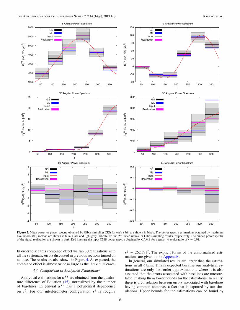
The mean posterior power spectra, together with the associ-ated uncertainties at each � bin, obtained by the methods of GSand ML for the ideal linear experiment, are shown in Figure 2.The input power spectra, which are used to construct the sig-nal realization, and the spectra of the signal realization are alsoshown in Figure 2. Almost all of our estimates fall within 2σ ofthe expected value.

5.2. Effect of Errors

In order to estimate α we ran 30 realizations of each sys-tematic error simulation for both linear and circular experi-ments. To keep the value of αr less than 10% tolerance limitat r = 0.01, we set the rms values of the parameters for gainerrors to |grms| = 0.1, for coupling errors to |εrms| = 5 × 10−4,for pointing errors to δrms ≈ 0.◦7, for beam shape errors toζrms ≈ 0.◦7, and for cross-polarization errors to μrms = 5×10−4.

Figure 3 shows the mean values of αXY for beam errors, aver-aged over 30 realizations. The results from ML and GS methodsare in good agreement for both linear and circular experiments.In all three cases αBB ∼ 0.1 at low �, as expected. Althoughthe cross polarization has a much smaller error parameter, itseffect on the power spectra is comparable to the pointing andshape errors. The reason for this is the leakage from T T powerinto BB power that is caused by the off-diagonal elements ofthe beam pattern, whereas the source of αBB for pointing andshape errors is the EE → BB leakage (Bunn 2007).

The mean values of αXY for instrumental errors are shownin Figure 4. For gain and coupling errors, αXY is roughly atthe 10% level. The main contribution for the αBB comes fromthe leakage from EE power into BB power for gain errors. Asin the case of cross-polarization errors, despite having a muchsmaller parameter than gain, αBB ∼ 0.1 at low � for antennacoupling errors because of T T → BB leakage.

We simulated the systematics by turning on one error at atime. However, in a realistic experiment, all systematic errors acttogether simultaneously, causing a larger effect on the spectra.

5

The Astrophysical Journal Supplement Series, 207:14 (14pp), 2013 July Karakci et al.

1000

2000

3000

4000

5000

6000

7000

50 100 150 200 250 300 350

ClT

T l(

l+1)

/ 2π

[μK

2 ]

l

TT Angular Power Spectrum

GSML

InputRealization

-60

-30

0

30

60

90

120

150

50 100 150 200 250 300 350

ClT

E l(

l+1)

/ 2π

[μK

2 ]

l

TE Angular Power Spectrum

GSML

InputRealization

0

5

10

15

20

25

50 100 150 200 250 300 350

ClE

E l(

l+1)

/ 2π

[ μK

2 ]

l

EE Angular Power Spectrum

GSML

InputRealization

0

0.01

0.02

0.03

0.04

0.05

50 100 150 200 250 300 350

ClB

B l(

l+1)

/ 2π

[μK

2 ]

l

BB Angular Power Spectrum

GSML

InputRealization

-4

-3

-2

-1

0

1

2

3

50 100 150 200 250 300 350

ClT

B l(

l+1)

/ 2π

[μK

2 ]

l

TB Angular Power Spectrum

GSML

InputRealization

-0.3

-0.2

-0.1

0

0.1

0.2

50 100 150 200 250 300 350

ClE

B l(

l+1)

/ 2π

[μK

2 ]

l

EB Angular Power Spectrum

GSML

InputRealization

Figure 2. Mean posterior power spectra obtained by Gibbs sampling (GS) for each � bin are shown in black. The power spectra estimations obtained by maximumlikelihood (ML) method are shown in blue. Dark and light gray indicate 1σ and 2σ uncertainties for Gibbs sampling results, respectively. The binned power spectraof the signal realization are shown in pink. Red lines are the input CMB power spectra obtained by CAMB for a tensor-to-scalar ratio of r = 0.01.

In order to see this combined effect we ran 30 realizations withall the systematic errors discussed in previous sections turned onat once. The results are also shown in Figure 4. As expected, thecombined effect is almost twice as large as the individual cases.

5.3. Comparison to Analytical Estimations

Analytical estimations for αXY are obtained from the quadra-ture difference of Equation (15), normalized by the numberof baselines. In general αXY has a polynomial dependenceon s2. For our interferometer configuration s2 is roughly

s2 ∼ 262.7/�2. The explicit forms of the unnormalized esti-mations are given in the Appendix.

In general, our simulated results are larger than the estima-tions in all � bins. This is expected because our analytical es-timations are only first order approximations where it is alsoassumed that the errors associated with baselines are uncorre-lated, making them lower bounds for the estimations. In reality,there is a correlation between errors associated with baselineshaving common antennas, a fact that is captured by our sim-ulations. Upper bounds for the estimations can be found by

6

The Astrophysical Journal Supplement Series, 207:14 (14pp), 2013 July Karakci et al.

δ=0.7 o Antenna Pointing Errors (TT & TE)

50 100 150 200 250 300 350Multipole l

0.01

0.10

αXY =

ΔC

l / σ

l

δ=0.7 o Antenna Pointing Errors (EE & BB)

50 100 150 200 250 300 350Multipole l

0.01

0.10

αXY =

ΔC

l / σ

l

δ=0.7 o Antenna Pointing Errors (TB & EB)

50 100 150 200 250 300 350Multipole l

0.01

0.10

αXY =

ΔC

l / σ

l

ζ=0.7 o Beam Shape Errors (TT & TE)

50 100 150 200 250 300 350Multipole l

0.01

0.10

1.00

αXY =

ΔC

l / σ

l

ζ=0.7 o Beam Shape Errors (EE & BB)

50 100 150 200 250 300 350Multipole l

0.1

1.0

αXY =

ΔC

l / σ

l

ζ=0.7 o Beam Shape Errors (TB & EB)

50 100 150 200 250 300 350Multipole l

0.01

0.10

αXY =

ΔC

l / σ

l

μ=5x10−4 Beam Cross Polarization (TT & TE)

50 100 150 200 250 300 350Multipole l

0.0001

0.0010

0.0100

αXY =

ΔC

l / σ

l

μ=5x10−4 Beam Cross Polarization (EE & BB)

50 100 150 200 250 300 350Multipole l

0.001

0.010

0.100

αXY =

ΔC

l / σ

l

μ=5x10−4 Beam Cross Polarization (TB & EB)

50 100 150 200 250 300 350Multipole l

0.001

0.010

0.100

αXY =

ΔC

l / σ

l

Figure 3. Beam errors. The values of αXY , averaged over 30 simulations, obtained by both maximum likelihood (ML) method (triangles) and the method of Gibbssampling (GS; solid dots) are shown. The three rows indicate, from top to bottom, pointing errors with δrms ≈ 0.◦7, beam shape errors with ζrms ≈ 0.◦7, and beamcross-polarization with μrms = 5 × 10−4. Left panel shows αT T (red) and αT E (blue). Middle panel shows αEE (red) and αBB (blue). Right panel shows αT B (red)and αEB (blue). Linear and circular experiments are shown by solid and dashed lines, respectively.

unrealistically assuming full correlation of errors between base-lines, where each baseline has the same error. For our inter-ferometer design, this corresponds to roughly 65 times largervalues. We expect our results to fall between uncorrelated andfully correlated estimations. In order to compare our results withthe analytical ones, we consider the rms values of αXY averagingover the � bins. Figure 5 shows the ratios of αXY

rms obtained byML and GS methods to the estimated αXY

rms. In most cases, bothmethods are in agreement with the analytical results within afactor of six.

5.4. Biases in Tensor-to-Scalar Ratio

The major goal of QUBIC-like experiments is to detect thesignals of the primordial B-modes, the magnitude of which ischaracterized by the tensor-to-scalar ratio r. In this context, it isnecessary to propagate the effects of systematic errors throughto r to assess properly the systematic-induced biases in theprimordial B-mode measurements.

The shape of the primordial BB power spectrum CBB�,prim is

insensitive to r but the amplitude is directly proportional to r. We

can straightforwardly convert the amplitude of the systematic-induced false BB into the bias in r by writing CBB

�,prim = rCBB�,r=1

in Equations (9) and (10) where CBB�,r=1 is the CAMB (Lewis et al.

2000) calculated primordial BB power spectrum at r = 1. Thetensor-to-scalar ratios obtained from an ideal linear experimentby GS and ML methods are found to be rGS = 0.026 ± 0.012and rML = 0.006 ± 0.0095, respectively. A more conservativeestimation for r can be obtained without subtracting the lensedspectrum in Equation (9) and by taking only the first bin wherethe effect of lensing is the least; r lensed

GS = 0.038 ± 0.014 andr lensed

ML = 0.0196 ± 0.011.We vary each systematic error individually and also consider

the cross contributions between each error. In realistic obser-vations, all different systematic errors are likely to occur at thesame time and we need to understand their combined effectswell. We thus evaluate such effects by simulating the system-atic errors occurring simultaneously during the observation. Theindividual and combined systematic-induced biases in r are il-lustrated in Figure 6, evaluated by both the GS and ML methodsbased on the simulations performed in the linear and circular

7

The Astrophysical Journal Supplement Series, 207:14 (14pp), 2013 July Karakci et al.

g=0.1 Antenna Gain Errors (TT & TE)

50 100 150 200 250 300 350Multipole l

0.01

0.10

αXY =

ΔC

l / σ

l

g=0.1 Antenna Gain Errors (EE & BB)

50 100 150 200 250 300 350Multipole l

0.01

0.10

αXY =

ΔC

l / σ

l

g=0.1 Antenna Gain Errors (TB & EB)

50 100 150 200 250 300 350Multipole l

0.01

0.10

1.00

αXY =

ΔC

l / σ

l

ε=5x10−4 Antenna Coupling Errors (TT & TE)

50 100 150 200 250 300 350Multipole l

0.0001

0.0010

0.0100

0.1000

αXY =

ΔC

l / σ

l

ε=5x10−4 Antenna Coupling Errors (EE & BB)

50 100 150 200 250 300 350Multipole l

0.001

0.010

0.100αX

Y =

ΔC

l / σ

l

ε=5x10−4 Antenna Coupling Errors (TB & EB)

50 100 150 200 250 300 350Multipole l

0.01

0.10

αXY =

ΔC

l / σ

l

Combined Systematic Errors (TT & TE)

50 100 150 200 250 300 350Multipole l

0.01

0.10

1.00

αXY =

ΔC

l / σ

l

Combined Systematic Errors (EE & BB)

50 100 150 200 250 300 350Multipole l

0.1

1.0

αXY =

ΔC

l / σ

l

Combined Systematic Errors (TB & EB)

50 100 150 200 250 300 350Multipole l

0.01

0.10

1.00

αXY =

ΔC

l / σ

l

Figure 4. Instrumental and combined systematic errors. The values of αXY , averaged over 30 simulations, obtained by both maximum likelihood (ML) method (triangles)and the method of Gibbs sampling (GS; solid dots) are shown. Top row: antenna gain with |grms| = 0.1. Middle row: antenna couplings with |εrms| = 5 × 10−4.Bottom row: combined effect of beam and instrumental systematic errors. Left panel shows αT T (red) and αT E (blue). Middle panel shows αEE (red) and αBB (blue).Right panel shows αT B (red) and αEB (blue). Linear and circular experiments are shown by solid and dashed lines, respectively.

bases. Both methods demonstrate good agreement, within a fac-tor of 2.5. Although the mock visibility data are simulated basedon only one realization of CMB anisotropy fields, drawn fromthe power spectra with input BB for r = 0.01, the resulting falseBB band-powers for the different systematic errors are expectedto be a good approximation for other r values since the leading-order false B-modes are contaminated only by the leakage ofT T , T E and EE power spectra, which are independent of r.

The simulations show that, due to the leakage of T T signalsinto BB, even though the cross-polarization and coupling errorsare very small, e.g., μrms = 5 × 10−4 and |εrms| = 5 × 10−4,the resulting biases in r are comparable to those induced byrelatively larger pointing, gain, and shape errors. In addition,when increasing the cross-polarization and coupling errors bya factor of 10, the simulations show that the resulting biaseswould roughly increase by the same factor. As expected, thesystematic errors are approximately linearly proportional totheir error parameters. We also find that the combined systematiceffects (referred to as “c” in Figure 6) would increase the biasesand their values are consistent with the quadrature sum of theindividual errors within 10%.

If we set up an allowable tolerance level of 10% on r, wherer is assumed to be r = 0.01, for QUBIC-like experiments theerror parameters adopted as in Figure 6 satisfy this thresholdwhen each systematic error occurs alone during observations.But if all the systematic errors are present at the same time, onaverage, we require roughly two times better systematic controlon each error parameter for a linear experiment. Nevertheless,the bias in r for a circular experiment, being around 15%, is stillwithin the acceptable level. Although the tolerance level for ris chosen to be αr = 0.1, our results can directly apply to anyother desired threshold level as long as the linear dependence ofsystematic effects on error parameters is a good approximationfor sufficiently small error parameters.

6. DISCUSSIONS

In this work a complete pipeline of simulations is de-veloped to diagnose the effects of systematic errors on theCMB polarization power spectra obtained by an interferomet-ric observation. A realistic, QUBIC-like interferometer designwith systematics that incorporate the effects of sky-rotation is

8

The Astrophysical Journal Supplement Series, 207:14 (14pp), 2013 July Karakci et al.

Figure 5. The bin-averaged ratios of the simulated and analytical systematic errors. In each panel, the results from the simulations in both the linear and circular basesfor T T , EE, BB, T E are shown. The gray and black bars correspond to the maximum-likelihood and Gibbs-sampling methods in analysis of the simulated data,respectively.

Figure 6. The simulated systematic-induced biases in the tensor-to-scalar ratio r (left) and αr (right) for the same systematic errors as in Figures 3 and 4. All the resultsderived from the maximum-likelihood (gray) and Gibbs-sampling (black) analyses based on the simulations in both the linear and circular bases are shown.

simulated. The mock data sets are analyzed by both the MLmethod and the method of GS. The results from both methodsare found to be consistent with each other, as well as with theanalytical estimations within a factor of six.

In order to assess the level at which systematic effects mustbe controlled, a tolerance level of αr = 0.1 is chosen. Thisensures that the instrument is sensitive enough to detect theB-signal at r = 0.01 level (O’Dea et al. 2007). We see that,

for a QUBIC-like experiment, the contamination of the tensor-to-scalar ratio at r = 0.01 does not exceed the 10% tolerancelevel in the multipole range 28 < � < 384 when the Gaussian-distributed systematic errors are controlled with precisions of|grms| = 0.1 for antenna gain, |εrms| = 5 × 10−4 for antennacoupling, δrms ≈ 0.◦7 for pointing, ζrms ≈ 0.◦7 for beam shape,and μrms = 5 × 10−4 for beam cross-polarization when eacherror acts individually. However, in a realistic experiment all the

9

The Astrophysical Journal Supplement Series, 207:14 (14pp), 2013 July Karakci et al.

systematic errors are simultaneously present, in which case thetolerance parameter of r roughly reaches the 20% level for thelinear experiment and 15% for the circular experiment. Althoughthis suggests that better control of systematics would be neededfor a linear experiment, for a QUBIC-like experiment withcircular polarizers, bias in r induced by combined systematicerrors would still be on the acceptable level when the systematicsare controlled with the given precisions.

Apart from the systematics presented in the paper, we alsoran simulations to analyze the effects of uncertainties in thepositions of the antennas. In order to have an effect on theorder of αBB = 0.1, we found that the uncertainty in the positionof each antenna should be on the order of 50% of the length ofthe uv plane. Since such an error is unrealistically large, weconclude that the effect of antenna position errors on powerspectra is negligible in an interferometric observation.

We have shown that a QUBIC-like experiment has fairlymanageable systematics, which is essential for the detection ofprimordial B-modes. Since our interferometer design has a largenumber of redundant baselines (approximately 10 baselines per

visibility), as a further improvement, a self-calibration techniquecan be employed to significantly reduce the level of instrumentalerrors (Liu et al. 2010; Keating et al. 2012).

Computing resources were provided by the University ofRichmond under NSF Grant 0922748. Our implementationof the Gibbs sampling algorithm uses the open-source PETSclibrary (Balay et al. 1997, 2010) and FFTW (Frigo & Johnson2005). G. S. Tucker and A. Karakci acknowledge supportfrom NSF Grant AST-0908844. P. M. Sutter and B. D.Wandelt acknowledge support from NSF Grant AST-0908902.B. D. Wandelt acknowledges funding from an ANR Chaired’Excellence, the UPMC Chaire International in TheoreticalCosmology, and NSF grants AST-0908902 and AST-0708849.L. Zhang and P. Timbie acknowledge support from NSF GrantAST-0908900. E. F. Bunn acknowledges support from NSFGrant AST-0908900. We are grateful for the generous hospital-ity of The Ohio State University’s Center for Cosmology andAstro-Particle Physics, which hosted a workshop during whichsome of these results were obtained.

APPENDIX

Following Bunn (2007), we obtain first order approximations for the ΔCXYrms given, for a single baseline, in Equation (15). For a

baseline lying on the x-axis, the matrices in Equation (15) are given as

NT T =(

1 0 00 0 00 0 0

), NEE = [(c2)2 − (s2)2]−1

⎛⎝0 0 00 c2 00 0 −s2

⎞⎠ , NBB = [(c2)2 − (s2)2]−1

⎛⎝0 0 00 −s2 00 0 c2

⎞⎠

NT E = 1

2c

(0 1 01 0 00 0 0

), NT B = 1

2c

(0 0 10 0 01 0 0

), NEB = 1

2(c2 − s2)

(0 0 00 0 10 1 0

).

The covariance matrix can be written in block-matrix form as Mw = (M0 M1M†

1 M2

)where

M0 =

⎛⎜⎝ CT T CT Ec CT Bc

CT Ec CEEc2 + CBBs2 CEB(c2 − s2)

CT Bc CEB(c2 − s2) CEEs2 + CBBc2

⎞⎟⎠ .

For a baseline lying in an arbitrary direction, these matrices must be transformed as M0 → R−1M0R and NXY → R−1NXY R, whereR is the rotation matrix given in Equation (14). The resulting expression will, then, be averaged over θ .

For instrumental errors δv = E · v, which gives M1 = M0 · E† and M2 = E · M0 · E†.

A.1. Gain Errors

g1 = 1

2

(gi

1 + gi2 + g

j∗1 + g

j∗2

), g2 = 1

2

(gi

1 − gi2 + g

j∗1 − g

j∗2

)

A.1.1. Linear Basis

γ1 = 1

2

(g

Q1 + gU

1

), γ2 = 1

2

(g

Q1 − gU

1

), γ3 = 1

2

(g

Q2 + gU

2

),

Egainlinear =

(γ1 γ3 00 γ1 + γ2 00 0 γ1 − γ2

)

10

The Astrophysical Journal Supplement Series, 207:14 (14pp), 2013 July Karakci et al.(ΔCT T

rms

)2 = 8Re{γ1}2(CT T )2(ΔCT E

rms

)2 = (6Re{γ1}2 + (3/4)Re{γ2}2 − (1/4)Im{γ2}2)(CT E)2 + (2Re{γ1}2 + (1/4)|γ2|2)CT T CEE(ΔCEE

rms

)2 = (8Re{γ1}2 + 4Re{γ2}2)(CEE)2(ΔCBB

rms

)2 = s2|γ2|2(CEE)2(ΔCT B

rms

)2 = (1/4)(3Re{γ2}2 − Im{γ2}2)(CT E)2 + (1/4)(|γ2|2 + 8Re{γ1}2)CT T CEE(ΔCEB

rms

)2 = Re{γ2}2(CEE)2 + (|γ2|2 + 2Re{γ1}2)CEECBB

A.1.2. Circular Basis

Egaincircular =

(g1 0 00 g1 ig20 −ig2 g1

)(ΔCT T

rms

)2 = 8Re{g1}2(CT T )2(ΔCT E

rms

)2 = 6Re{g1}2(CT E)2 + 2Re{g1}2CT T CEE(ΔCEE

rms

)2 = 8Re{g1}2(CEE)2(ΔCBB

rms

)2 = 2|g2|2CEE(CBB + s2CEE)(ΔCT B

rms

)2 = ((3/2)Im{g2}2 − (1/2)Re{g2}2)(CT E)2 + (1/2)|g2|2CT T CEE(ΔCEB

rms

)2 = 2Im{g2}2(CEE)2

A.2. Coupling Errors

e1 = 1

2

(ei

1 + ei2 + e

j∗1 + e

j∗2

), e2 = 1

2

(ei

1 − ei2 − e

j∗1 + e

j∗2

)

A.2.1. Linear Basis

ε1 = 1

2

(eQ1 + eU

1

), ε2 = 1

2

(eQ1 − eU

1

), ε3 = 1

2

(eQ2 + eU

2

), ε4 = 1

2

(eQ2 − eU

2

),

Ecouplinglinear =

(0 0 ε1

ε1 + ε2 0 −ε3 − ε4ε1 − ε2 ε3 − ε4 0

)(ΔCT T

rms

)2 = (3Re{ε1}2 − Im{ε1}2)(CT E)2 + |ε1|2CT T CEE(ΔCT E

rms

)2 = 2(Re{ε1}2 + Re{ε2}2)(CT T )2(ΔCEE

rms

)2 = 2(|ε1|2 + |ε2|2)CT T CEE(ΔCBB

rms

)2 = 2(|ε1|2 + |ε2|2)CT T CBB + 2s2(|ε1|2 + |ε2|2)CT T CEE(ΔCT B

rms

)2 = 2(Re{ε1}2 + Re{ε2}2)(CT T )2(ΔCEB

rms

)2 = (1/2)(|ε1|2 + |ε2|2)CT T CEE + (1/2)(3Re{ε1}2 + 3Re{ε2}2 − Im{ε1}2 − Im{ε2}2)(CT E)2

A.2.2. Circular Basis

Ecouplingcircular =

(0 e1 ie2e1 0 0ie2 0 0

)(ΔCT T

rms

)2 = (3Re{e1}2 − Im{e1}2 + 2Im{e2}2)(CT E)2 + (|e1|2 + |e2|2)CT T CEE(ΔCT E

rms

)2 = (Re{e1}2 + Im{e2}2)((CT T )2 + (CT E)2 + CT T CEE)(ΔCEE

rms

)2 = (3Re{e1}2 − Im{e1}2 + 2Im{e2}2)(CT E)2 + (|e1|2 + |e2|2)CT T CEE(ΔCBB

rms

)2 = (|e1|2 + |e2|2)CT T (CBB + s2CEE)(ΔCT B

rms

)2 = (Re{e1}2 + Im{e2}2)(CT T )2(ΔCEB

rms

)2 = (1/4)(|e1|2 + |e2|2)CT T CEE + (1/4)(3Re{e1}2 + 3Im{e2}2 − Im{e1}2 − Re{e2}2)(CT E)2

11

The Astrophysical Journal Supplement Series, 207:14 (14pp), 2013 July Karakci et al.

A.3. Pointing Errors

Defining δrk as the deviation of the kth antenna’s pointing center, we can write, to the first order,

Aj (r)Ak(r) = exp[−(r − σδ)2/2σ 2],

where δ = (δrj + δrk)/2σ.

δVZ = −iσ

∫d2kZ(k)

[A2

0(k − 2πu)]∗

[(k − 2πu) · δZ]

〈VXδV ∗Y 〉 = 0 and 〈δVXδV ∗

Y 〉 = (1/2)(δX · δY )〈VXV ∗Y 〉.

A.3.1. Linear Basis

δ1 = 1

2(δQ + δU ), δ2 = 1

2(δQ − δU )

(ΔCT T

rms

)2 = |δ1|2(CT T )2(ΔCT E

rms

)2 = (1/2)|δ1|2(CT E)2 + (1/8)(4|δ1|2 + |δ2|2)CT T CEE(ΔCEE

rms

)2 = (|δ1|2 + (1/2)|δ2|2)(CEE)2(ΔCBB

rms

)2 = |δ1|2CBB(CBB + 2s2CEE) + (1/2)|δ2|2CEE(CBB + s2CEE)(ΔCT B

rms

)2 = (1/2)|δ1|2CT T (CBB + s2CEE) + (1/8)|δ2|2CT T CEE(ΔCEB

rms

)2 = (1/2)|δ1|2CEE(CBB + s2CEE) + (1/8)|δ2|2(CEE)2

A.3.2. Circular Basis

δ2 = 0

A.4. Shape Errors

The product of two elliptic Gaussian beams can be written as a single elliptic Gaussian:

Aj (r)Ak(r) = exp

[− (x cos β + y sin β)2

2(σ + σx)2− (y cos β − x sin β)2

2(σ + σy)2

],

where β is the angle between the major axis of the resulting ellipse and the x-axis.

δVZ = − 1

σ 2

∫d2kZ(k)

[(A2

0ΔZ

)(k − 2πu)

]∗

where ΔZ(x, y) = x2(ζZx cos2 β + ζZ

y sin2 β) + y2(ζZy cos2 β + ζZ

x sin2 β) + xy(ζZx − ζZ

y ) sin 2β, and ζZx,y = σZ

x,y/σ.The only non-vanishing integrals in the covariance matrix are:∫

|A2|2 = πσ 2,

∫A2(x2A2)∗ =

∫A2(y2A2)∗ = 1

2πσ 4,

∫|x2A2|2 =

∫|y2A2|2 = 3

4πσ 6,

∫(x2A2)(y2A2)∗ =

∫|xyA2|2 = 1

4πσ 6.

ζ Z1 = 1

2

(ζZx + ζZ

y

), ζ Z

2 = 1

2

(ζZx − ζZ

y

); ζi+ = 1

2

(ζ

Qi + ζU

i

), ζi− = 1

2

(ζ

Qi − ζU

i

)Averaging over β we get 〈VXδV ∗

Y 〉 = −ζ Y1 〈VXV ∗

Y 〉 and 〈δVXδV ∗Y 〉 = (2ζX

1 ζ Y1 + ζX

2 ζ Y2 )〈VXV ∗

Y 〉.

12

The Astrophysical Journal Supplement Series, 207:14 (14pp), 2013 July Karakci et al.

A.4.1. Linear Basis(ΔCT T

rms

)2 = (10ζ 2

1+ + 2ζ 22+

)(CT T )2(

ΔCT Erms

)2 = (7ζ 2

1+ + (3/4)ζ 21− + ζ 2

2+

)(CT E)2 +

(3ζ 2

1+ + (1/2)ζ 21− + ζ 2

2+ + (1/4)ζ 22−

)CT T CEE(

ΔCEErms

)2 = (10ζ 2

1+ + 5ζ 21− + 2ζ 2

2+ + ζ 22−

)(CEE)2(

ΔCBBrms

)2 = (2ζ 2

1− + ζ 22−

)s2(CEE)2 +

(12ζ 2

1+ + 12ζ 21− + 4ζ 2

2+ + ζ 22−

)s2CEECBB +

(10ζ 2

1+ + 5ζ 21− + 2ζ 2

2+ + ζ 22−

)(CBB)2(

ΔCT Brms

)2 = (3/4)ζ 21−(CT E)2 + (1/4)

(2ζ 2

1− + ζ 22−

)CT T CEE +

(3ζ 2

1+ + (1/2)ζ 21− + ζ 2

2+ + (1/4)ζ 22−

)s2CT T CEE(

ΔCEBrms

)2 = ((5/4)ζ 2

1− + (1/4)ζ 22− + s2

(3ζ 2

1+ + ζ 22+

))(CEE)2

A.4.2. Circular Basis

ζi− = 0

A.5. Cross-polarization

The only non-vanishing integrals in the covariance matrix are:∫|A2|2 = πσ 2,

∫| ˜A2ρ2 cos 2φ|2 =

∫| ˜A2ρ2 sin 2φ|2 = πσ 6.

A.5.1. Linear Basis

μ1 = 1

2(μQ + μU ), μ2 = 1

2(μQ − μU )

δI = μ1ρ2

σ 2(Q cos 2φ + U sin 2φ), δQ = (μ1 + μ2)

ρ2

σ 2I cos 2φ, δU = (μ1 − μ2)

ρ2

σ 2I sin 2φ

(ΔCT T

rms

)2 = 2μ21C

T T CEE(ΔCT E

rms

)2 = (1/2)(μ2

1 + μ22

)(CT T )2(

ΔCEErms

)2 = 2(μ2

1 + μ22

)CT T CEE(

ΔCBBrms

)2 = 2(μ2

1 + μ22

)CT T (CBB + s2CEE)(

ΔCT Brms

)2 = (1/2)(μ2

1 + μ22

)(CT T )2(

ΔCEBrms

)2 = (1/2)(μ2

1 + μ22

)CT T CEE

A.5.2. Circular Basis

μ+ = 1

2(μi + μj ), μ− = 1

2(μi − μj )

δI = μ+ρ2

σ 2Q sin 2φ, δQ = μ+

ρ2

σ 2I sin 2φ + iμ−

ρ2

σ 2U cos 2φ, δU = −iμ−

ρ2

σ 2Q cos 2φ

(ΔCT T

rms

)2 = μ2+C

T T CEE(ΔCT E

rms

)2 = (1/4)μ2+(CT T )2(

ΔCEErms

)2 = (μ2+C

T T − 2μ2−CEE)CEE(

ΔCBBrms

)2 = (μ2+C

T T − 2μ2−CEE)(CBB + s2CEE)(

ΔCT Brms

)2 = (1/4)(μ2+C

T T − 2μ2−CEE)CT T(

ΔCEBrms

)2 = (1/4)(μ2+C

T T − 2μ2−CEE)CEE

REFERENCES

Baker, J. C., Grainge, K., Hobson, M. P., et al. 1999, MNRAS, 308, 1173Balay, S., Gropp, W. D., McInnes, L. C., & Smith, B. F. 1997, in Modern

Software Tools for Scientific Computing, ed. E. Arge, A. M. Bruaset, & H.P. Langtangen (Boston, MA: Birkhauser), 163

Balay, S., Gropp, W. D., McInnes, L. C., & Smith, B. F. 2010, PETScUsers Manual, Rev. 3.1 (Argonne, IL: Argonne National Laboratory),http://www.mcs.anl.gov/petsc/

Bond, J., Jaffe, A. H., & Knox, L. 1998, PhRvD, 57, 2117Bunn, E. F. 2007, PhRvD, 75, 083517Bunn, E. F. 2011, PhRvD, 83, 083003Bunn, E. F., & White, M. 1997, ApJ, 480, 6Dickinson, C., Battye, R. A., Carreira, P., et al. 2004, MNRAS, 353, 732Fomalont, E. B., Kellermann, K. I., Wall, J. V., & Weistrop, D. 1984, Sci,

225, 23Frigo, M., & Johnson, S. 2005, IEEEP, 93, 216Gelman, A., & Rubin, D. 1992, StaSc, 7, 457

13

The Astrophysical Journal Supplement Series, 207:14 (14pp), 2013 July Karakci et al.

Gorski, K. M., Banday, A. J., Bennett, C. L., et al. 1996, ApJL, 464, L11Grainge, K., Carreira, P., Cleary, K., et al. 2003, MNRAS, 341, L23Hinshaw, G., Larson, D., Komatsu, E., et al. 2012, arXiv:1212.5226Hobson, M. P., & Magueijo, J. 1996, MNRAS, 283, 1133Hobson, M., & Maisinger, K. 2002, MNRAS, 334, 569Hu, W., & Dodelson, S. 2002, ARA&A, 40, 171Hu, W., Hedman, M. M., & Zaldarriaga, M. 2003, PhRvD, 67, 043004Kamionkowski, M., Kosowsky, A., & Stebbins, A. 1997, PhRvL, 78, 2058Karakci, A., Sutter, P. M., Zhang, L., et al. 2013, ApJS, 204, 8Keating, B., Shimon, M., & Yadav, A. 2012, ApJL, 762, L23Knoke, J. E., Partridge, R. B., Ratner, M. I., & Shapiro, I. I. 1984, ApJ, 284, 479Komatsu, E., Smith, K. M., Dunkley, J., et al. 2011, ApJS, 192, 18Kovac, J. M., Leitch, E. M., Pryke, C., et al. 2002, Natur, 420, 772Larson, D., Dunkley, J., Hinshaw, G., et al. 2011, ApJS, 192, 16Larson, D. L., Eriksen, H. K., Wandelt, B. D., et al. 2007, ApJ, 656, 653Lewis, A., Challinor, A., & Lasenby, A. 2000, ApJ, 538, 473Liu, A., Tegmark, M., Morrison, S., Lutomirski, A., & Zaldarriaga, M.

2010, MNRAS, 408, 1029Martin, H. M., Partridge, R. B., & Rood, R. T. 1980, ApJL, 240, L79Miller, N., Shimon, M., & Keating, B. 2009, PhRvD, 79, 063008Myers, S. T., Contaldi, C. R., Bond, J. R., et al. 2003, ApJ, 591, 575Myers, S. T., Sievers, J. L., Bond, J. R., et al. 2006, Natur, 50, 951

Ng, K.-W. 2005, PhRvD, 71, 083009O’Dea, D., Challinor, A., & Johnson, B. 2007, MNRAS, 376, 1767O’Sullivan, C., Yassin, G., Woan, G., et al. 1995, MNRAS, 274, 861Park, C.-G., & Ng, K.-W. 2004, ApJ, 609, 15Park, C.-G., Ng, K.-W., Park, C., Liu, G.-C., & Umetsu, K. 2003, ApJ,

589, 67Partridge, R. B., Nowakowski, J., & Martin, H. M. 1988, Natur, 331, 146Pearson, T. J., Mason, B. S., Readhead, A. C. S., et al. 2003, ApJ, 591, 556Qubic Collaboration, Battistelli, E., Bau, A., et al. 2011, APh, 34, 705Scott, P. F., Saunders, R., Pooley, G., et al. 1996, ApJL, 461, L1Shimon, M., Keating, B., Ponthieu, N., & Hivon, E. 2008, PhRvD, 77, 083003Stuart, A., & Ord, J. 1987, Kendall’s Advanced Theory of Statistics (5th ed.;

Hoboken, NJ: Wiley)Su, M., Yadav, A. P., Shimon, M., & Keating, B. G. 2011, PhRvD, 83, 103007Sutter, P., Wandelt, B. D., & Malu, S. 2012, ApJS, 202, 9Takahashi, Y. D., Ade, P. A. R., Barkats, D., et al. 2010, ApJ, 711, 1141Timbie, P. T., Tucker, G. S., Ade, P. A. R., et al. 2006, NewAR, 50, 999Timbie, P. T., & Wilkinson, D. T. 1988, RScI, 59, 914White, M., Carlstrom, J. E., Dragovan, M., & Holzapfel, W. L. 1999, ApJ,

514, 12Yadav, A. P., Su, M., & Zaldarriaga, M. 2010, PhRvD, 81, 063512Zhang, L., Karakci, A., Sutter, P. M., et al. 2012, ApJS, 206, 24

14